International Trade and Retailing∗

Carsten Eckel

University of Bamberg†

November 10, 2008

Abstract

The New Trade Theory predicts that international trade lowers prices for consumers

and raises the choices available to them. This study shows that both predictions may no

longer hold once adjustments in retailing are taken into account. We present a new model

of retailing in general equilibrium and establish a trade-off between the number of products

stocked and the number of retail outlets. The results demonstrate that international trade

can lead to higher consumer prices if the retail market is relatively less competitive, and

that retail assortments do not rise if consumers have a sufficiently low preference for

diversity.

Keywords: International Trade, Retailing, Diversity, Market Structure, Welfare, Mo-

nopolistic Competition.

JEL Classification: F12, L11, L81

∗I gratefully acknowledge research support from the German Science Foundation (DFG grant number EC216/5-1). Thanks also to Jim Anderson, Beata Javorcik, James Markusen, J. Peter Neary, Volker Nocke,Michael Pflüger, Horst Raff, and Michael Rauscher for helpful comments and discussions. A previous versionof this paper circulated with the subtitle "Diversity versus Accessibility and the Creation of ’Retail Deserts’"and was presented at various conferences and seminars.

†University of Bamberg, Department of Economics, Feldkirchenstr. 21, D-96052 Bamberg, Ger-many; tel.: (+49) 951-863-2583; e-mail: carsten.eckel@uni-bamberg.de; home page: http://www.uni-bamberg.de/sowi/eckel.

i

1 Introduction

The modern theory of international trade identifies an expansion in the choices for consumers

and an increase in their real income as the key gains from trade (Krugman, 1979, 1980,

for the seminal theoretical contributions; Broda and Weinstein, 2006, for a recent empirical

investigation). These propositions are based on adjustments in the market structures of man-

ufacturing industries. International trade enlarges the markets for manufacturers and makes

their operations more profitable, so that the equilibrium number of firms in an integrated

global economy is larger than the number of firms in any national economy under autarky. As

a consequence, product diversity rises and consumers can choose from a larger menu of differ-

entiated varieties. In addition, demand becomes more elastic and firms can realize economies

of scale, so that producer prices fall and real incomes rise.

Changes in the market structure of manufacturing industries are important for consumers,

but they are only one part of the story. Typically, consumers do not buy their products

directly from manufacturers but travel to local retail outlets for their purchases. Hence, the

choices available to consumers and the prices paid are also affected by the market structure

in retailing, in particular by the local availability of retail outlets, by the assortment sizes of

local retailers and by the retail mark-ups. Whether consumers can choose from a larger range

of products at lower prices depends upon whether local retailers find it profitable to expand

the number of products in their assortment and how retail mark-ups change. Thus, for a full

assessment of the impact of international trade on a country’s welfare we have to take into

account how the market structure in retailing is affected.

Surprisingly, the retail sector has received very little attention in the theory of interna-

tional trade. Previous studies on international trade and retailing have focused either on

strategic issues between manufacturers and retailers in partial equilibrium (Richardson, 2004;

Raff and Schmitt, 2005, 2006, 2007), or on the role of intermediaries in overcoming informa-

tional barriers in international markets (Rauch, 2001; Rauch and Casella, 2003; Feenstra and

Hanson, 2004). This lack of attention is particularly striking since the retail industries in most

industrialized countries have gone through immens structural changes over the past decades

that have had an equally immens impact on the local availability of manufactured products.

There is overwhelming evidence that the level of concentration has increased significantly and

1

that the overall number of retail outlets has declined (Dobson and Waterson, 1999; Clarke,

2000; Dawson, 2001; Dobson et al., 2001; Blanchard and Lyson, 2002, 2003; Weiss and Wit-

tkopp, 2005; U.S. Department of Commerce, 2006). At the same time, the average number

of products stocked in supermarkets has risen significantly (Competition Commission, 2000;

Richards and Hamilton, 2006) and the number of gigantic supermarkets, so-called superstores,

has even increased in absolute terms despite the overall decline in retail outlets (Dobson et

al., 2001; Dobson et al., 2003). In addition, there is evidence that retail gross margins have

risen (Dobson et al., 1998; Dobson and Waterson, 1999, Competition Commission, 2000; U.S.

Census Bureau, 2008). Today, the retail sectors in many countries are characterized by larger

and more profitable but fewer retail outlets than some decades ago.

This paper establishes a link between international trade in monopolistically competi-

tive industries and the market structure in retailing in a general equilibrium framework. It

addresses two questions: First, how can international trade contribute to the recent develop-

ments in the retail industries? And second, in how far do these adjustments in the retailing

industries alter our prediction regarding the welfare implications of international trade? By

incorporating a retailing sector into an otherwise standard general equilibrium model of intra-

industry trade we will be able to isolate mechanisms through which international trade can

affect the market structure in retailing and calculate their welfare implications. I want to

state clearly upfront that I do not claim that international trade is solely responsible for these

developments in the retailing industries. These industries have been affected by many differ-

ent shocks simultaneously, such as increases in consumer mobility, changing shopping habits

or technological progress (internet). However, I do argue that international trade is a distinct

force in these developments, and that the adjustments triggered in the retailing industries

have to be taken into account when assessing the welfare implications of international trade.

We will see that a retail equilibrium implies a trade-off between product diversity and retail

density, and that because of this trade-off international trade can actually lower a country’s

welfare.

The model presented here takes the general setup of a Krugman (1979, 1980)-type model of

intra-industry trade with regard to consumer preferences (Dixit-Stiglitz) and manufacturing

firms (horizontally differenciated, with fixed and variable labor costs) and adds a spatial

2

component for the retailing industry based on the monocentric city model à la Alonso (1964)

and the spatial model by Salop (1979) used in industrial organization. The economy has a

circular structure where consumers (who are also workers) live on a circle around a Central

Business District (CBD) and travel to the nearest local retailer for their purchases. The

modeling of retailing, in particular the modeling of a retailer’s cost function builds on recent

contributions in industrial organization and agricultural economics, in particular on Sullivan

(1997), Smith (2004), Ellickson (2006, 2007), and Richards and Hamilton (2006), as well

as on an industry study by the UK Competition Commission (2000). Retailers can locate

freely anywhere on the circumference of this circle and make four distinct decisions: (1)

Whether to enter or not, (2) where to locate, (3) what mark-ups to charge, and (4) how many

products to offer. Under some circumstances, the retailers will also charge slotting fees from

manufacturing firms. Because the market structure in retailing is determined endogenously,

this framework allows us to study how international trade affects not only retail prices but

also the equilibrium number of retailers, their catchment areas and assortment sizes.

The base model is described in great detail in the next section. Then we conduct three

comparative static exercises: International trade in the form of an increase in the number of

countries integrated in the global economy (section 3), internal economic growth in the form

of an increase in the labor supply and an increase in consumer mobility in the form of a fall

in travel costs for consumers (section 4). In section 5 we show that when consumers have a

very low preference for diversity, retailers have an incentive to limit the number of products

stocked. This leads to the payment of slotting allowances and changes the way the economy

adjusts to shocks. Finally, we present a number of extensions to the base model that illustrate

how the framework can accommodate asymmetries or address policy issues.

2 A General Equilibrium Model of Retailing

Let us begin by outlining the geographical structure of our framework (Figure 1). Suppose

that the economy of a country is populated by a mass of L consumers who live on a circle

with circumference Ω around a central business district (CBD). The mass of consumers is

uniformly distributed across the circumference of this circle, so that the population density is

identical at all points and given by L/Ω.

3

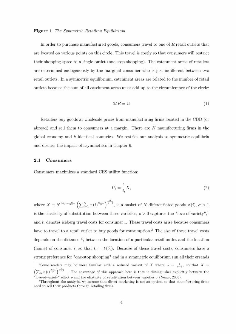
Figure 1 The Symmetric Retailing Equilibrium

In order to purchase manufactured goods, consumers travel to one of R retail outlets that

are located on various points on this circle. This travel is costly so that consumers will restrict

their shopping spree to a single outlet (one-stop shopping). The catchment areas of retailers

are determined endogenously by the marginal consumer who is just indifferent between two

retail outlets. In a symmetric equilibrium, catchment areas are related to the number of retail

outlets because the sum of all catchment areas must add up to the circumference of the circle:

2δR = Ω (1)

Retailers buy goods at wholesale prices from manufacturing firms located in the CBD (or

abroad) and sell them to consumers at a margin. There are N manufacturing firms in the

global economy and k identical countries. We restrict our analysis to symmetric equilibria

and discuss the impact of asymmetries in chapter 6.

2.1 Consumers

Consumers maximizes a standard CES utility function:

Uι =1

tιX, (2)

where X ≡ N1+ρ− σσ−1

³PNi=1 x (i)

σ−1σ

´ σσ−1 , is a basket of N differentiated goods x (i), σ > 1

is the elasticity of substitution between these varieties, ρ > 0 captures the "love of variety",1

and tι denotes iceberg travel costs for consumer ι. These travel costs arise because consumers

have to travel to a retail outlet to buy goods for consumption.2 The size of these travel costs

depends on the distance δι between the location of a particular retail outlet and the location

(home) of consumer ι, so that tι = t (δι). Because of these travel costs, consumers have a

strong preference for "one-stop shopping" and in a symmetric equilibrium run all their errands

1Some readers may be more familiar with a reduced variant of X where ρ = 1σ−1 , so that X =

N x (i)σ−1σ

σσ−1

. The advantage of this approach here is that it distinguishes explicitly between the

"love-of-variety" effect ρ and the elasticity of substitution between varieties σ (Neary, 2003).2Throughout the analysis, we assume that direct marketing is not an option, so that manufacturing firms

need to sell their products through retailing firms.

4

in a single shopping trip (Stahl, 1987; Competition Commission, 2000; Smith and Hay, 2005).

We assume that travel costs are convex and use the following specific functional form:

tι = exp (τδι) . (3)

The retail outlets are located on various points on the circumference of the circle, so that the

distance δι can be expressed as the shortest arcdistance between the home of the consumer

and the location of the retail outlet. Note that (3) implies tι (0) = 1 and d ln tι/d ln δι = τδι >

0. The parameter τ is a technological parameter that captures all exogenous influences on

consumer travel costs, like infrastructure and consumer mobility.

Each consumer/worker household supplies one unit of labor. We use labor as our numeraire

so that the wage rate and a houshold’s income is normalized to one. Then, maximization of

(2) subject to the budget constraintP

N p (i)x (i) ≤ 1 yields demand for individual varieties

of X:

x (i) = p (i)−σ P σ−1. (4)

Here, P ≡ Nσ

σ−1−1−ρ³P

N p (i)1−σ´ 11−σ is the price index of the composite good X. We

assume that N is large, but not large enough for consumers to disregard the price index effect

(Yang and Heijdra, 1993). Hence, the value of the price elasticity of demand is given by

−d lnx (i) /d ln p (i) = σ + (1− σ) [p (i) /P ]1−σ, which reduces to

−d lnxd ln p

= σ

µ1− 1

N

¶+1

N(5)

in a symmetric equilibrium. The price elasticity is a weighed average of the substitution effect

(σ) and the income effect (1), and its value rises when N rises. The consideration of the

price index effect is important for two reasons. First and foremost, it provides a rationale

for retailers to offer sales on individual items in order to make a retail outlet more attractive

for consumers. Second, it eliminates the unsatisfactory result that the mark-up charged by

manufacturing firms is unaffected by the degree of competition (Yang and Heijdra, 1993).

5

2.2 Manufacturing

Manufacturing firms produce single varieties of the differentiated good under increasing re-

turns to scale.3 Their profits are given by

ΠM = (pW − β)Q− α, (6)

where α and β denote the fixed and variable labor requirements, pW is the wholesale price

and Q denotes world market demand.

International trade is free and there are no trade costs associated with exporting to foreign

markets. World market demand comes from a mass of L consumers in k identical countries.

Hence,

Q = kLx. (7)

Because retailers charge a mark-up μ, retail prices differ from wholesale prices:

p = (1 + μ) pW . (8)

The mark-up charged by retailers has no influence on the perceived price elasticity of man-

ufacturing firms as they treat the retail mark-up as given. Hence, from the perspective of a

manufacturing firm: d ln pW/d lnx = d ln p/d lnx. Then, given equations (5), (6) and (7), the

profit maximizing wholesale price is

pW = β

∙1 +

N

(σ − 1) (N − 1)

¸. (9)

Note that the mark-up charged by manufacturing firms (pW/β − 1) depends on the elasticity

of substitution between varieties (σ) and on the number of manufacturing firms in the global

economy (N). The mark-up falls when N rises because demand becomes more elastic when

the number of competitors rises.

Manufacturing firms enter or exit the global market until profits are driven down to zero.

Using (4), (6), (7), (8) and (9), the condition for a free-entry profit-maximizing equilibrium

3The analysis is limited to symmetric equilibria and indices are supressed for simplicity.

6

in the manufacturing industry is

kL = α (1 + μ) (σN − σ + 1) . (10)

2.3 Retailing

Retailers buy products from manufacturers at the wholesale price pW and sell them with a

mark-up (8) to local consumers. The profits of a retailer j are given by

ΠR (j) = 2δjL

Ω

NjXi=1

[p (i)− pW ]x (i)− γNj (11)

The first term on the right hand side of (11) denotes a retailer’s gross profits. They consist

of gross profits per consumerPNj

i=1 [p (i)− pW ]x (i) times population density L/Ω over its

catchment area 2δj , where δj captures the catchment area to one side of its location on the

circle.

The second term, γNj , is the labor requirement necessary to provide Nj goods. We will

refer to these costs as the costs of provision. The costs of provision depend positively on the

number of varieties in the assortment (Competition Commission, 2000, in particular chaper

10 and its appendix), but are sunk in the sense that once a retailer has decided upon its

product assortment, the costs of providing these goods do not depend on the actual sales.

One can think of these costs as expenditures for in-store service personnel or labor services in

departments such as purchasing or storage (Sullivan, 1997).4 Equation (11) does not exhibit

any marginal costs of retailing. Their relevance is limited with respect to the mechanisms

described here, so we can safely ignore them.

Given the utility of consumers and their "love of variety", the product assortment offered

by a retailer can be interpreted as an index of the quality of a retail outlet (Ellickson, 2006,

2007). A trip to a retail outlet with a larger assortment of products allows a consumer to

purchase a larger variety of goods and realize a higher utility. Hence, our model can be

interpreted as a model with both vertical (quality) and horizontal (location) differentiation.

Retailers maximize profits by choosing the optimal mark-up μ. In a symmetric equilibrium,

4More complex specifications for the costs of provision lead to qualitatively similar results as long as thenumber of varieties remains an independent argument in the cost function.

7

the profit-maximizing mark-up is identical across all products and retailers and satisfies (see

Appendix 8.1)

μ = − 1N

µd ln δ

d lnμ

¶−1− 1. (12)

Note that the profit-maximizing mark-up does not depend on the price elasticity of in-

dividual products [equation (5)], but solely on the elasticity of the retailers catchment area

(d ln δ/d lnμ). This is because, in contrast to (single-product) manufacturing firms, retailing

firms sell a basket of goods and internalize demand linkages between these goods. A reduction

in the price of one product may increase revenues on this product, but with a binding budget

constraint consumers must finance the extra expenditures through a reduction in expendi-

tures on other products. This is known as the "cannibalization effect" and it is particularly

relevant in the context of retailing. Here, "cannibalization" is perfect in the sense that con-

sumers spend their entire income at a single retail outlet (one-stop shopping), so that their

expenditures are equal to their income (which is normalized to one) and independent of the

mark-up charged by the retail outlet [P

N p (i)x (i) = 1].

For a retailer, "cannibalization" implies that inframarginal revenues (from sales to cus-

tomers within a retailer’s catchment area) are independent of the retailer’s mark-up. However,

changes in the mark-up do affect a retailer’s external margin, i.e. its catchment area. A higher

mark-up makes a retail outlet less attractive to consumers and reduces the retailer’s catch-

ment area. This is why the profit-maximizing mark-up in (12) depends on the elasticity of

the catchment area δ.

The elasticity of the catchment area can be calculated by looking at the marginal consumer

who is just indifferent between two retail outlets. Given (2), (4) and (9), the elasticity of the

catchment area with respect to a retailer’s mark-up is

d ln δ

d lnμ= − 1

N

μ

(1 + μ)

1

2δτ. (13)

In a symmetric equilibrium, the mark-up is identical across products and retailers, and the

catchment areas of all retail outlets must cover the circumference of the circle. By substituting

(13) into (12) and using (1) we can express the optimal mark-up as a function of the mobility

8

of consumers (τ) and the density of retail outlets (R/Ω):5

μ =τΩ

R. (14)

An increase in either the mobility of consumers (a fall in τ) or the density of retail outlets (an

increase in R/Ω) reduces the local monopoly power of a retailer and leads to a lower mark-up.

There is free entry in retailing, too. Hence, in equilibrium retail profits are zero: ΠR = 0.

Using equations (1), (11) and (14), the zero profit condition can be expressed as

τΩ

R+ τΩL = RγN . (15)

Note that we use the same symbol N for the product assortment of a retailer and for the

number of manufacturing firms and that the latter is determined by the zero profit condition

(10) in manufacturing. Hence, we implicitly assume that retailers take all products available

on the world market into their assortments. This is not trivial because providing products is

costly for retailers and we need to make sure that they do not find it profitable to restrict

their assortment. Technically, this implies that dΠR (j) /d lnNj is positive when evaluated at

zero profits. For the moment, we simply assume that this condition is satisfied and treat the

retailers’ assortments as being determined by the zero profit condition in manufacturing. We

will come back to this in section 5 where we discuss the implications of this assumptions and

how the equilibrium is determined when this condition is not satisfied.

2.4 The General Equilibrium

Equations (10), (14) and (15) determine the retail mark-up μ, the number of manufacturing

firms N and the number of retailers R. Wholesale and retail prices (in units of labor, pW and

p) as well as the real wage (1/p) are then given by (9) and (8), and consumption and output

levels by (4) and (7). The labor market is in equilibrium as well. Let national labor markets

be perfectly competitive and completely segregated. The supply of labor is exogenously

given by the number of consumers/workers L. The demand for labor consists of demand

5Equation (13) shows the impact of a change in an individual mark-up on the catchment area. If a retailervaries all mark-ups symmetrically, the impact is N times as high. Thus, the term 1/N disappears in thecalculation of (14).

9

for manufacturing (N/k) (α+ βQ) and demand for retailing (RγN). Using the equilibrium

values for N , R and Q, we find that labor markets are in equilibrium, too:

N

k(α+ βQ) +RγN =

µNpWx+

μ

1 + μ

¶L = L (16)

In order to illustrate the equilibrium graphically we reduce the system of equations to

two equations in the number of manufacturing firms N and the number of retailers R. The

first of these two is the zero profit condition in the retailing industry (15). The second

equation is derived by substituting the retail mark-up (14) into the zero profit condition in

the manufacturing industry (10):

kL = α

µ1 +

τΩ

R

¶(σN − σ + 1) . (17)

The equilibrium is illustrated in Figure 2. The upward sloping curve is the zero profit

condition in the manufacturing industry (ΠmaxM = 0). The downward sloping curve represents

the zero profit condition in the retailing industry (ΠmaxR = 0).

Figure 2 The General Equilibrium

The two zero profit conditions in Figure 2 highlight an important difference in the relation-

ship between manufacturing firms and retailers. Retailers are the "friends" of manufacturing

firms in the sense that profits in manufacturing are increasing in the number of retailing firms.

The reason for this is that an increase in the number of retailers lowers retail mark-ups, and

this boost consumer demand for manufacturing products. The reverse relationship has the

opposite effect: Manufacturing firms are the "enemies" of retailers. An increase in the supply

of differentiated manufacturing products raises the retailers’ costs of provision, and this cost

increase leads to a consolidation in the retailing industry. Hence, the zero profit condition in

the retail industry creates a trade-off between diversity (the number of products offered) and

the retail density.

10

3 International Trade

Let us think of international trade as an enlargement of the global market in the form of

an increase in the number of countries integrated in the global economy (an increase in k).

Graphically, the manufacturing zero profit condition (ΠmaxM = 0) shifts to the right. This

shift resembles the traditional result of the new trade theory: For a given market structure

in retailing (R = R), an increase in the global market clearly raises the number of firms and,

thus, the number of differentiated products available for consumption. Note, however, that N

rises by less than k in relative terms: d lnN/d ln k|ΠmaxM =0

R=R= (σN − σ + 1) / (σN) < 1. Hence,

the number of firms per country, N/k, falls. There are two effects: First, an increase in k

implies a larger demand (and a larger labor supply to satisfy demand), so that the aggregate

number of firms supported in the global market rises. Second, the accompanying increase in

the number of differentiated products makes demand more elastic, so that all firms have to

lower their mark-ups. Consequently, firm output rises and the increase in the number of firms

is less than proportionate to the increase in the size of the global market.

The retailing zero profit condition is not directly affected by an increase in k. Technically,

this can be checked by confirming that equation (15) is indeed independent of k. Intuitively,

the retailing equilibrium is not affected because retailers sell ony locally and compete only

against other local retailers. Hence, an increase in the size of the global market has no direct

effect on the market structure in retailing.

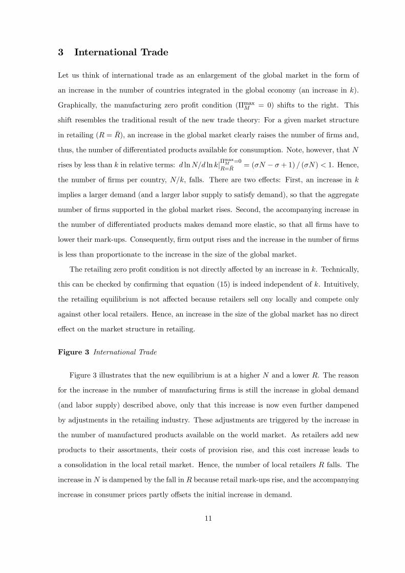
Figure 3 International Trade

Figure 3 illustrates that the new equilibrium is at a higher N and a lower R. The reason

for the increase in the number of manufacturing firms is still the increase in global demand

(and labor supply) described above, only that this increase is now even further dampened

by adjustments in the retailing industry. These adjustments are triggered by the increase in

the number of manufactured products available on the world market. As retailers add new

products to their assortments, their costs of provision rise, and this cost increase leads to

a consolidation in the local retail market. Hence, the number of local retailers R falls. The

increase in N is dampened by the fall in R because retail mark-ups rise, and the accompanying

increase in consumer prices partly offsets the initial increase in demand.

11

Mathematically, we obtain the following solutions (see Appendix 8.2):

d lnR

d ln k= − 1

∆< 0,

d lnN

d ln k=1

∆

(2R+ τΩ)

(R+ τΩ)> 0, (18)

where ∆ ≡ (2R+τΩ)(R+τΩ)

σN(σN−σ+1)+

τΩ(R+τΩ) > 1. The mathematical solutions confirm our graphical

analysis. In particular, they proof that the number of retailers falls and that the increase

in the number of manufacturing firms is less pronounced than without adjustments in the

retailing industry. This latter point can be seen by rearranging d lnN/d ln k in (18): d lnNd ln k =

1∆(2R+τΩ)(R+τΩ) =

³σN

σN−σ+1 +τΩ

2R+τΩ

´−1<³

σNσN−σ+1

´−1< 1.

Proposition 1 International trade leads to a fall in the number of local retailers. The ag-

gregate number of manufacturing firms in the global economy rises.

The changes in the retail mark-up and the wholesale prices follow from (14) and (9):

d lnμ

d ln k=1

∆> 0,

d ln pWd ln k

= − 1∆

N (2R+ τΩ)

(N − 1) (σN − σ + 1) (R+ τΩ)< 0. (19)

As equation (14) shows, the retail mark-up is inversely proportionally related to the num-

ber of retailers. Hence, as the number of retailers falls, and the distance between retailers

grows [d ln δ = −d lnR because of (1)], the local monopoly power of retailers rises. As a

consequence, retailers are able to raise their mark-ups. On the other side, wholesale prices

and mark-ups in manufacturing fall even though the number of manufacturing firms per coun-

try has fallen, too (d lnN/d ln k < 1). But in contrast to retailers, manufacturing firms are

competing globally and their mark-ups depend on the degree of competition in the global

economy. And because the aggregate number of manufacturing firms rises, demand becomes

more elastic and manufacturers are forced to lower their prices.

Proposition 2 International trade raises the mark-ups in retailing while mark-ups in man-

ufacturing fall.

The results in (19) convey an important message. The manufacturing industry and the re-

tailing industry are affected in a fundamentally different way by international trade. Because

manufacturing firms compete globally, they are confronted with a more competitive environ-

ment when new countries join the global market. Retailers compete only locally. Therefore,

12

they are only indirectly affected through a larger availability of manufactured products world-

wide. Because this raises their costs of provision, some retailers have to exit, and the remaining

retailers face a less competitive environment. As a consequence of these diverse effects, the

mark-ups in manufacturing fall and those in retailing rise.

The fact that retail mark-ups rise is not only interesting in itself, it is also highly relevant

for the impact of international trade on consumer prices. One of the potential gains from trade

that is frequently cited from the textbook theory is that international trade lowers prices for

consumers. We have seen that wholesale prices fall indeed, but consumer (or retail) prices

(p) depend on retail mark-ups, too. And with retail mark-ups rising, the total impact on

consumer prices is ambiguous.

The mathematical solution for the impact on consumer prices can be derived from (8):

d ln p

d ln k=

μ

1 + μ

d lnμ

d ln k+

d ln pWd ln k

=

hσ (N − 1)2 − 1

iτΩ− 2NR

∆ (R+ τΩ) (N − 1) (σN − σ + 1)T 0. (20)

Obviously, equation (20) can be either positive or negative, depending, among other variables,

on the market structures in retailing and in manufacturing, R and N . If R > τΩ2N [σ (N − 1)

2−

1], then d ln p/d ln k < 0 and vice versa.

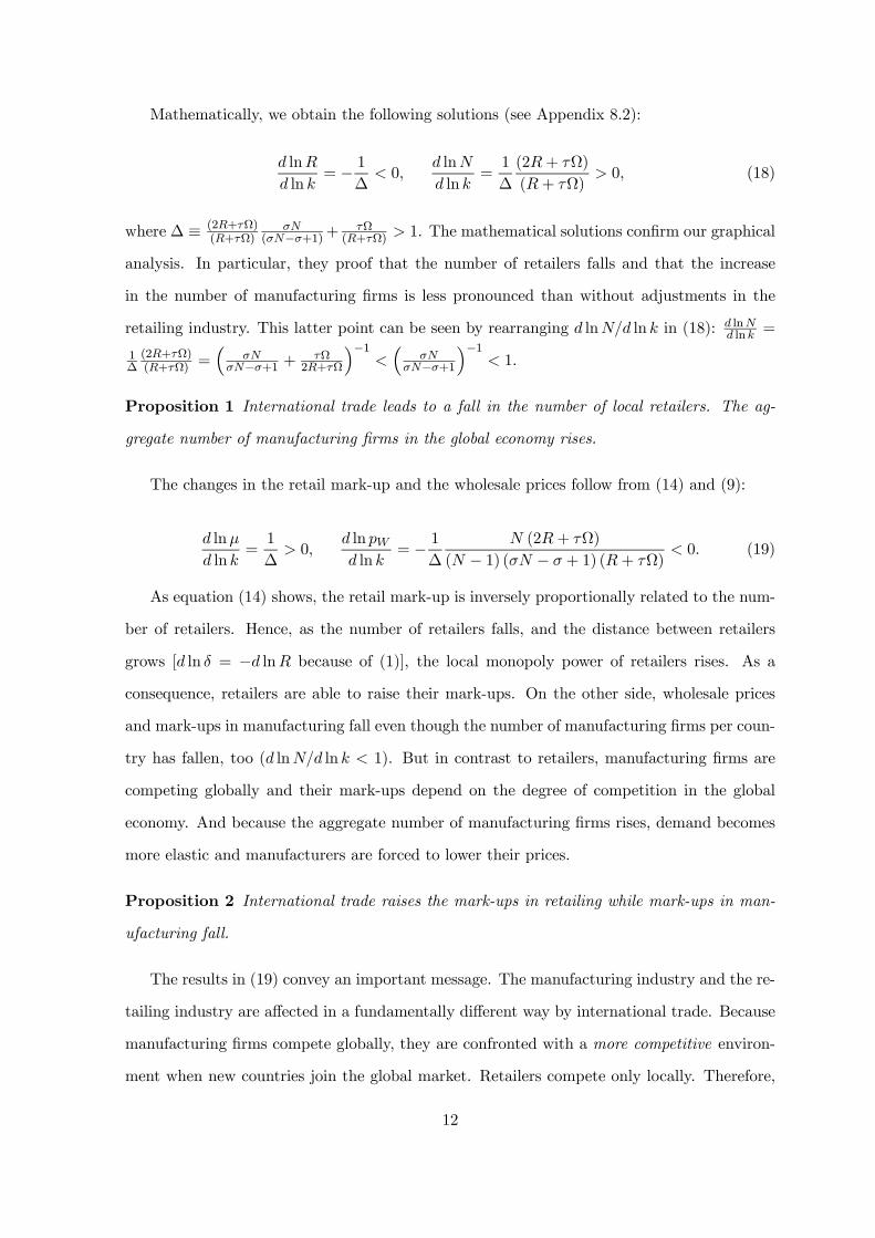
Figure 4 The Effect on Consumer Prices

Figure 4 illustrates that consumer prices fall when the retail market is relatively compet-

itive compared to the manufacturing industry and rise when the manufacturing industry is

relatively more competitive. The reason for why relative competitiveness in the two indus-

tries matters for the impact of international trade on consumer prices is because it affects

the size of the adjustments in the mark-ups of these two industries. The more competitive

an industry is, the less mark-ups will respond to changes in the market structure. Take for

example the Dixit-Stiglitz approximation: If N →∞, mark-ups in manufacturing are essen-

tially fixed by the elasticity of substitution σ. In this case, wholesale prices do not fall at

all, and the rise in the retail mark-up translates directly into an increase of consumer prices:

limN→∞d ln pd ln k =

12

τΩR+τΩ > 0.

Since we use labor as our numeraire, the real wage is given by the inverse of consumer

prices (1/p). Therefore, when consumer prices rise, the real wage falls and vice versa. This

13

implies that as a result of the adjustments in the retail industry, international trade can

actually lower real wages.

Proposition 3 The impact of international trade on consumer prices and on the real wage is

ambiguous. The real wage falls if mark-ups in manufacturing are low compared to mark-ups

in retailing.

Finally, let us address the welfare effects of international trade. The fact that real wages

may fall is an important first step in this direction, but consumer do not only value real

income, they also value diversity. In addition, there are travel costs that depend on the

the consumer’s distance to the nearest retail outlet. Because these travel costs depend on a

consumer’s location, individual utility levels differ. Average utility is defined as U ≡ 1δ

R δ0 Uιdι

and, given (2), can be expressed as U = Nρ/¡pt¢, where t is the harmonic mean of travel

costs t ≡ δ³R δ0 (tι)

−1 dι´−1

. The relative change in average utility is

d ln U = ρd lnN − d ln p− d ln t. (21)

Equation (21) nicely illustrates the three factors determining the relative change in average

utility: The first term (ρd lnN) is the love-of-variety effect. It depends on the relative change

in the number of varieties (d lnN) weighed by the consumers’ preference for diversity (the

parameter ρ). The second term is the relative change in the real wage (−d ln p) and the third

term is the relative change in mean travel costs (d ln t).

The last term, the relative change in mean travel costs, depends on changes in the size

of the catchment area (δ) and on changes in the mobility of consumers (τ). Since there is a

strictly inverse relationship between catchment areas and the number of retailers [equation

(1)], a consolidation in retailing will raise mean travel costs. Given (3), the relative change in t

can be expressed as d ln t = − t(δ)−tt(δ) (d lnR− d ln τ), where t(δ)−t

t(δ) = 1− τδ¡eτδ − 1

¢−1 ∈ (0, 1)can be interpreted as a measure of the relative curvature of travel costs.

The total impact of international trade on average utility is given by d ln Ud ln k = ρd lnNd ln k −

d ln pd ln k −

d ln td ln k and is ambiguous. The first term on the right hand side, the love-of-variety effect,

is clearly positive. The last term, the travel cost effect, is clearly negative. And the term in

the middle, the change in the real wage, is itself ambiguous.

14

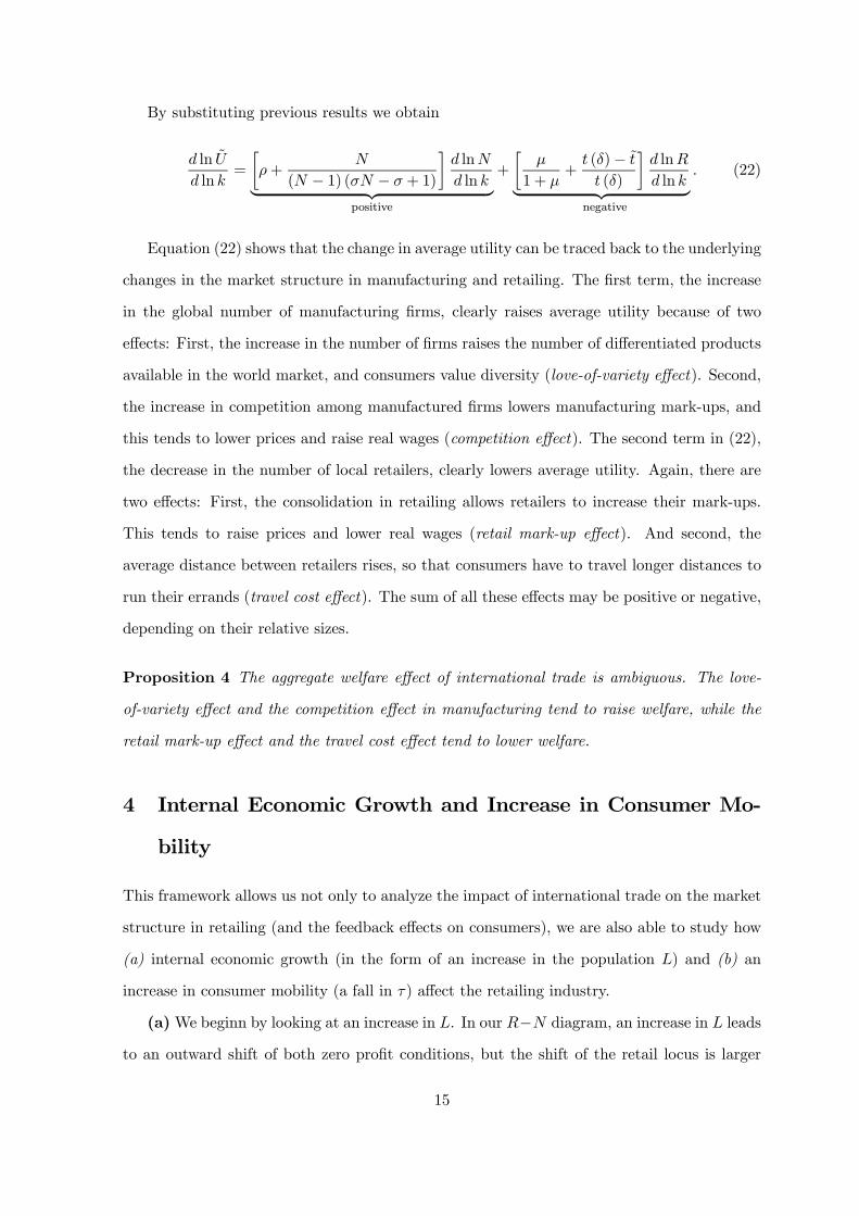
By substituting previous results we obtain

d ln U

d ln k=

∙ρ+

N

(N − 1) (σN − σ + 1)

¸d lnN

d ln k| z positive

+

∙μ

1 + μ+

t (δ)− t

t (δ)

¸d lnR

d ln k| z .negative

(22)

Equation (22) shows that the change in average utility can be traced back to the underlying

changes in the market structure in manufacturing and retailing. The first term, the increase

in the global number of manufacturing firms, clearly raises average utility because of two

effects: First, the increase in the number of firms raises the number of differentiated products

available in the world market, and consumers value diversity (love-of-variety effect). Second,

the increase in competition among manufactured firms lowers manufacturing mark-ups, and

this tends to lower prices and raise real wages (competition effect). The second term in (22),

the decrease in the number of local retailers, clearly lowers average utility. Again, there are

two effects: First, the consolidation in retailing allows retailers to increase their mark-ups.

This tends to raise prices and lower real wages (retail mark-up effect). And second, the

average distance between retailers rises, so that consumers have to travel longer distances to

run their errands (travel cost effect). The sum of all these effects may be positive or negative,

depending on their relative sizes.

Proposition 4 The aggregate welfare effect of international trade is ambiguous. The love-

of-variety effect and the competition effect in manufacturing tend to raise welfare, while the

retail mark-up effect and the travel cost effect tend to lower welfare.

4 Internal Economic Growth and Increase in Consumer Mo-

bility

This framework allows us not only to analyze the impact of international trade on the market

structure in retailing (and the feedback effects on consumers), we are also able to study how

(a) internal economic growth (in the form of an increase in the population L) and (b) an

increase in consumer mobility (a fall in τ) affect the retailing industry.

(a)We beginn by looking at an increase in L. In our R−N diagram, an increase in L leads

to an outward shift of both zero profit conditions, but the shift of the retail locus is larger

15

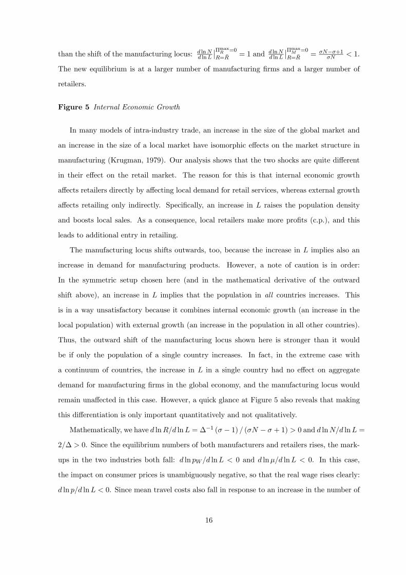
than the shift of the manufacturing locus: d lnNd lnL

¯ΠmaxR =0

R=R= 1 and d lnN

d lnL

¯ΠmaxM =0

R=R= σN−σ+1

σN < 1.

The new equilibrium is at a larger number of manufacturing firms and a larger number of

retailers.

Figure 5 Internal Economic Growth

In many models of intra-industry trade, an increase in the size of the global market and

an increase in the size of a local market have isomorphic effects on the market structure in

manufacturing (Krugman, 1979). Our analysis shows that the two shocks are quite different

in their effect on the retail market. The reason for this is that internal economic growth

affects retailers directly by affecting local demand for retail services, whereas external growth

affects retailing only indirectly. Specifically, an increase in L raises the population density

and boosts local sales. As a consequence, local retailers make more profits (c.p.), and this

leads to additional entry in retailing.

The manufacturing locus shifts outwards, too, because the increase in L implies also an

increase in demand for manufacturing products. However, a note of caution is in order:

In the symmetric setup chosen here (and in the mathematical derivative of the outward

shift above), an increase in L implies that the population in all countries increases. This

is in a way unsatisfactory because it combines internal economic growth (an increase in the

local population) with external growth (an increase in the population in all other countries).

Thus, the outward shift of the manufacturing locus shown here is stronger than it would

be if only the population of a single country increases. In fact, in the extreme case with

a continuum of countries, the increase in L in a single country had no effect on aggregate

demand for manufacturing firms in the global economy, and the manufacturing locus would

remain unaffected in this case. However, a quick glance at Figure 5 also reveals that making

this differentiation is only important quantitatively and not qualitatively.

Mathematically, we have d lnR/d lnL = ∆−1 (σ − 1) / (σN − σ + 1) > 0 and d lnN/d lnL =

2/∆ > 0. Since the equilibrium numbers of both manufacturers and retailers rises, the mark-

ups in the two industries both fall: d ln pW/d lnL < 0 and d lnμ/d lnL < 0. In this case,

the impact on consumer prices is unambiguously negative, so that the real wage rises clearly:

d ln p/d lnL < 0. Since mean travel costs also fall in response to an increase in the number of

16

retailers (d ln t/d lnR < 0), the welfare effect of an increase in L is unambiguously positive:

d ln U

d lnL= ρ

d lnN

d lnL| z (+)

− d ln p

d lnL| z (−)

− d ln t

d lnL| z (−)

> 0. (23)

Proposition 5 Internal economic growth raises the number of both retailers and manufactur-

ers. Mark-ups in both industries fall and the real wage as well as welfare rise unambiguously.

The core difference between an increase in the number of countries in the global economy

(k) and an increase in the size of the population (L) is that the former has no direct impact

on the retailing industry whereas the latter affects retailers directly through an increase in

local sales.

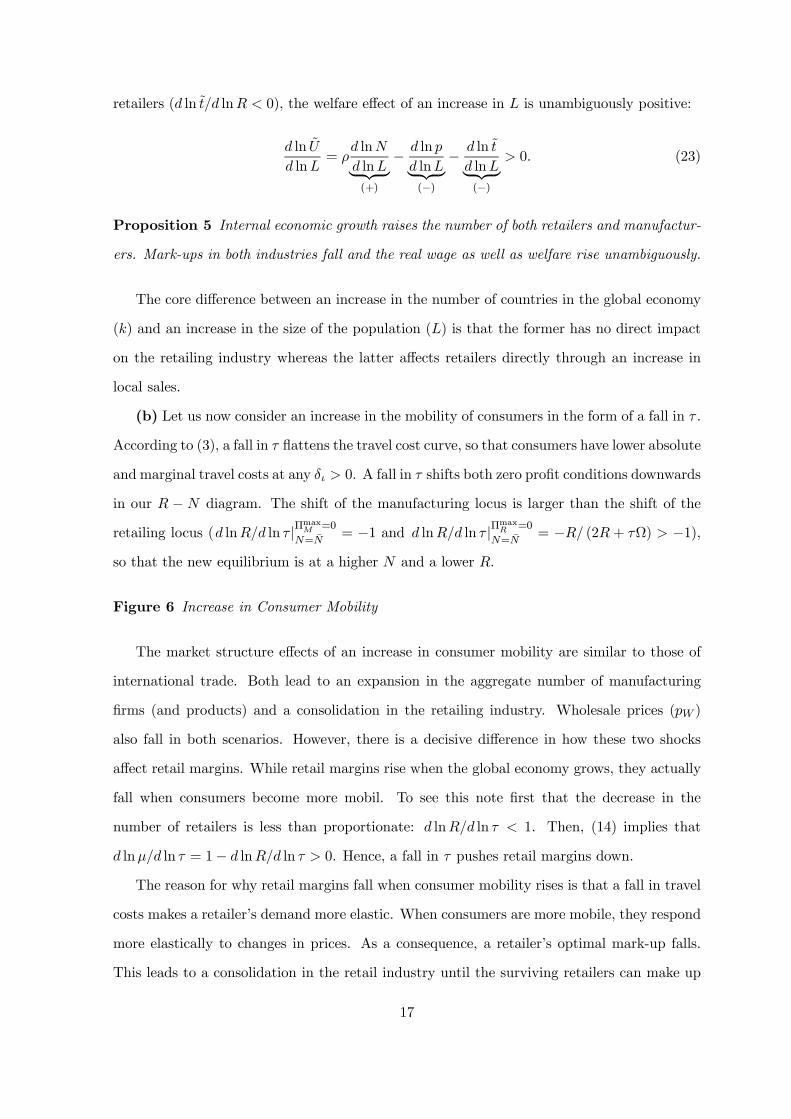
(b) Let us now consider an increase in the mobility of consumers in the form of a fall in τ .

According to (3), a fall in τ flattens the travel cost curve, so that consumers have lower absolute

and marginal travel costs at any δι > 0. A fall in τ shifts both zero profit conditions downwards

in our R − N diagram. The shift of the manufacturing locus is larger than the shift of the

retailing locus (d lnR/d ln τ |ΠmaxM =0

N=N= −1 and d lnR/d ln τ |Π

maxR =0

N=N= −R/ (2R+ τΩ) > −1),

so that the new equilibrium is at a higher N and a lower R.

Figure 6 Increase in Consumer Mobility

The market structure effects of an increase in consumer mobility are similar to those of

international trade. Both lead to an expansion in the aggregate number of manufacturing

firms (and products) and a consolidation in the retailing industry. Wholesale prices (pW )

also fall in both scenarios. However, there is a decisive difference in how these two shocks

affect retail margins. While retail margins rise when the global economy grows, they actually

fall when consumers become more mobil. To see this note first that the decrease in the

number of retailers is less than proportionate: d lnR/d ln τ < 1. Then, (14) implies that

d lnμ/d ln τ = 1− d lnR/d ln τ > 0. Hence, a fall in τ pushes retail margins down.

The reason for why retail margins fall when consumer mobility rises is that a fall in travel

costs makes a retailer’s demand more elastic. When consumers are more mobile, they respond

more elastically to changes in prices. As a consequence, a retailer’s optimal mark-up falls.

This leads to a consolidation in the retail industry until the surviving retailers can make up

17

in catchment areas what they lost in margins.

An increase in consumer mobility leads to a consolidation in the retail sector because it

lowers retail margins by raising the price elasticity of demand. This is a demand side shock.

An increase in the number of countries integrated in the global economy leads to higher retail

margins because the increase in the costs of provision lead to a consolidation in the retail

sector. This is a supply side shock. Therefore, even though both shock have the same impact

on the market structure in retailing, their impact on mark-ups is distinctly different.

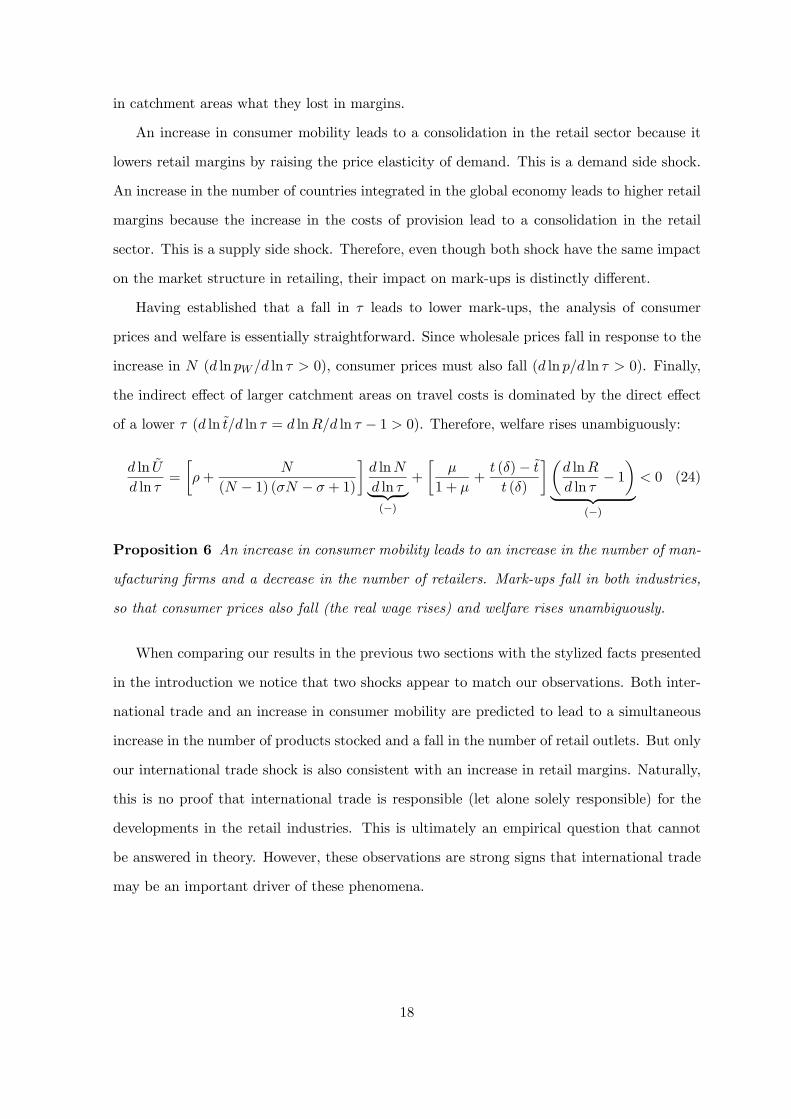
Having established that a fall in τ leads to lower mark-ups, the analysis of consumer

prices and welfare is essentially straightforward. Since wholesale prices fall in response to the

increase in N (d ln pW/d ln τ > 0), consumer prices must also fall (d ln p/d ln τ > 0). Finally,

the indirect effect of larger catchment areas on travel costs is dominated by the direct effect

of a lower τ (d ln t/d ln τ = d lnR/d ln τ − 1 > 0). Therefore, welfare rises unambiguously:

d ln U

d ln τ=

∙ρ+

N

(N − 1) (σN − σ + 1)

¸d lnN

d ln τ| z (−)

+

∙μ

1 + μ+

t (δ)− t

t (δ)

¸µd lnR

d ln τ− 1¶

| z (−)

< 0 (24)

Proposition 6 An increase in consumer mobility leads to an increase in the number of man-

ufacturing firms and a decrease in the number of retailers. Mark-ups fall in both industries,

so that consumer prices also fall (the real wage rises) and welfare rises unambiguously.

When comparing our results in the previous two sections with the stylized facts presented

in the introduction we notice that two shocks appear to match our observations. Both inter-

national trade and an increase in consumer mobility are predicted to lead to a simultaneous

increase in the number of products stocked and a fall in the number of retail outlets. But only

our international trade shock is also consistent with an increase in retail margins. Naturally,

this is no proof that international trade is responsible (let alone solely responsible) for the

developments in the retail industries. This is ultimately an empirical question that cannot

be answered in theory. However, these observations are strong signs that international trade

may be an important driver of these phenomena.

18

5 Assortment Sizes and Slotting Allowances

In section 2.3 we assumed that retailers find it always profitable to add products to their

assortments when they become available on the world market. We have already pointed out

that this assumption is not trivial because the provision of goods is costly. In this section we

want to discuss the conditions under which this assumption is valid and how the equilibrium

is determined when retailers want to restrict their assortment sizes.

First, we calculate the profit maximizing product assortment of a retailer by assuming

that retailers choose mark-ups and assortments simultaneously. An increase in a retailer’s

assortment raises its costs of provision, but it also makes this retail outlet more attractive

for consumers because it offers more choices. These two effects must be weighed off against

each other. The profit maximizing assortment size (denoted by an asterisk) N∗ and the

corresponding equilibrium number of retailers R∗ as well as their mark-ups μ∗ are then given

by

N∗ =ρ2L

(1 + ρ) γτΩ, R∗ =

τΩ

ρand μ∗ = ρ. (25)

In a symmetric equilibrium, the assortment size in retailing must be identical to the num-

ber of manufacturing firms in the global economy.6 Hence, the profit maximizing product

assortment in retailing and the zero profit condition in manufacturing are two competing con-

ditions for the determination of N , only one of which can be binding. The profit maximizing

assortment is binding if ρ is below a certain threshold ρ < ρ, where ρ > 0.7 If consumers have

a high "love of variety" (ρ > ρ), they respond strongly in their outlet decisions to changes in

a retailer’s assortment size. In this case, retailers find it profitable to take as many products

as possible into their assortments and the number of manufactured products is determined

by the zero profit condition in manufacturing. But if consumers have a low "love of variety"

(ρ < ρ), they look primarily for low retail prices. In that case, the costs of adding products to

a retailer’s assortment dominate the advantage of a larger assortment, so that retailers find

it profitable to limit the range of products offered.

If the profit maximizing assortment is binding (ρ < ρ), retailing firms create an arti-

6Because of economies of scale, a manufacturer serving all retailers can alway charge a price below theaverage costs of a manufacturer serving only a subset of retailers. Therefore, in equilibrium all manufacturingproducts are listed with all retailers.

7See equation (46) in Appendix 8.4.

19

ficial bottleneck that generates scarcity rents for manufacturing firms because the number

of products listed in the retail assortment is smaller and the wholesale price is higher than

in the equilibrium with zero profits. However, these scarcity rents cannot be appropriated

by the manufacturers. Without barriers to entry, manufacturing firms not listed will find it

profitable to offer "slotting allowances"8 to retailers in order to have their products placed

on their shelves. The ensuing competition between manufacturers for the scarce retail shelve

space raises these slotting allowances until profits in manufacturing are driven down to zero.

The payment of slotting allowances by manufacturing firms to retailers suggests that the

scarcity rents are passed on to the retailing firms. However, for the same reason these rents

cannot be appropriated by retailers, either. Without barriers to entry in retailing, retailers are

not only competing against their neighboring rivals, they are also competing against potential

entry at their own location. Hence, the slotting allowances paid by manufacturing firms are

passed on to final consumers.

In reality, slotting allowances usually take the form of either cash payments or free

goods. Here, it is most convenient to think of slotting allowances as of the "iceberg" type,

i.e. manufacturing firms ship out a larger quantity of goods than what they get paid for:

ΠM (i) = (pW (i)− βs (i))Q (i)−α, where s (i) > 1 are the iceberg slotting allowances. Note,

however, that in contrast to transportation costs, slotting allowances are not variable costs

but fixed payments in units of goods. As a type of market entry fee they do not enter into

the firm’s pricing decision, so that the wholesale price pW (i) continues to be determined by

equation (9).

Technically, we assume that manufacturing firms choose prices and slotting allowances

simultaneously. While final consumers perceive the various manufactured products as dif-

ferentiated and care about the diversity offered by local retailers, they do not care about

the composition of this diversity. Hence, when it comes to adding varieties to a retailer’s

assortment, the different manufactured products are essentially perfect substitutes. As a con-

sequence, the competition between manufacturers for the scarce retail space is Bertrand in

nature and slotting allowances rise until effective prices (net of slotting allowances, pW/s) are

8“’Slotting allowances’ are one class of payments that may be made for shelf access. They are lump-sum,up-front payments from a manufacturer (...) to a retailer to have a new product carried by the retailer andplaced on its shelves." (Federal Trade Commission, 2001).

20

down to average costs. The equilibrium slotting allowances are given by (see Appendix 8.4):

s∗ =

∙1− (1 + ρ)

αN∗

kL

¸σ (N∗ − 1) + 1(σ − 1) (N∗ − 1) . (26)

Consumers are the beneficiaries of these slotting allowances. For every unit they purchase

they get s − 1 units for free ("take one, get s − 1 for free" offers). Average utility is then

given by U = Nρ (s/p) /t, where s/p is the effective real wage (including slotting allowances):

s/p =£1− (1 + ρ) αN

∗

kL

¤/ [(1 + ρ)β].

We see that if the profit maximizing assortment is binding, the determination of the

equilibrium is quite different. It also has profound effects on how the markets respond to

shocks:

Proposition 7 International trade: If consumers have a low "love of variety" (ρ < ρ), an

increase in the number of countries (k) has no impact on the market structure in retailing or

in manufacturing. However, consumer are better off because of larger slotting allowances.

From the explicit solutions of N∗, R∗ and μ∗ in (25) it is immediately obvious that all three

parameters are unaffected by changes in k. Just as in the previous section there is no direct

effect of a change in k on the retailing sector because retailers sell only locally. But in contrast

to the previous section, there is no indirect effect via entry in the manufacturing industry,

either, because the equilibrium number of manufacturing products and firms is determined

in the retailing sector as well. An increase in k still makes manufacturing more profitable,

but this does not lead to entry but to an increase in slotting allowances. Log differentiation

of (26) yields d ln s∗/d ln k = (1 + ρ) αN∗

kL /£1− (1 + ρ) αN

∗

kL

¤> 0. As a consequence, average

utility rises even though N , p and t all remain constant: d ln U/d ln k = d ln s∗/d ln k > 0.

This is an important result. It shows that a larger international market does not necessarily

lead to an increase in the local choices for consumers. This depends on whether local retailers

find it profitable to expand their assortments. If they do, we have seen in the previous section

that this may lead to a consolidation in the retailing industry with ambiguous welfare effects.

If they don’t, then the analysis in this section shows that market structures and prices in both

retailing and manufacturing remain unaffected. However, consumers are better off because

they benefit from the fiercer global competition between manufacturers for the scarce retail

21

space that leads to an increase in slotting allowances.

Note that the result of locally constant assortments does not contradict studies empha-

sizing the growth in imported varieties (e.g., Broda and Weinstein, 2006). In our symmetric

setup, the share of imported varieties is given by (k − 1) /k, and this is clearly increasing

in k irrespective of how the market structure in manufacturing adjusts. In the case where

assortments remain constant, an increase in k leads to a proportional decrease in N/k. Hence,

an increase in the share of imported varieties leads to a change in the composition in local

retail assortments. However, our results also indicate that one must exercise extreme caution

when drawing welfare implications from the fact that more varieties are imported.

Analyzing other shocks (internal growth, mobility) is also straightforward:

Proposition 8 (a) Internal growth: An increase in L leads to larger assortments and higher

slotting allowances, but leaves the market structure in retailing unaffected. (b) Mobility: A fall

in τ leads to larger assortments and a consolidation in the retailing sector. Slotting allowances

fall.

Proof. Log differentiation of (25) and (26) yields (a) d lnN∗/d lnL = 1, d lnR∗/d lnL = 0,

and d ln s∗/d lnL > 0; (b) d lnN∗/d ln τ = −1, d lnR∗/d ln τ = 1, and d ln s∗/d ln τ > 0.

We see that shocks that have a direct impact on the retailing sector also have an impact

on the size of the assortments. An increase in L raises local demand for retailing services, and

this leads to a corresponding increase in the size of assortments. A fall in τ reduces travel

costs and makes demand for retailing services more elastic. This leads to a consolidation

in the retailing sector that in turn allows retailers to increase their assortment sizes. These

results are qualitatively similar to the results in the previous section.

6 Extensions

This framework can be extended in various directions. Following Melitz (2003), a by now

popular extension is to introduce heterogeneity in the productivity of manufacturing firms.

In principal, this could be done here as well, but would not lead to new insights regarding

the adjustments in the retailing industry.9 Instead, we focus on two asymmetries that have9Because of complete cannibalization, neither retail mark-ups nor assortment sizes depend on the costs in

manufacturing. Hence, introducing heterogeneous manufacturers leads to the well know selection effects in

22

a direct impact on the retailing industries: Consumers’ preference for diversity and zoning

regulations. In addition, we present a simple extension with a market for housing and rents.

6.1 Asymmetric Preferences for Diversity

Suppose that all countries are identical except for their consumers’ "love of variety", so that

the parameter ρ = ρ (i) is country specific. Then, countries with a high ρ are governed by

the regime described in section 2.4 and countries with a low ρ are governed by the regime

described in the previous section. The critical country k is determined in Figure 7, where

κ (ρ) is the sum of all countries with a ρ (i) ≥ ρ, and ρ (k) is taken from equation (46) in

Appendix 8.4. We will refer to the countries with a high "love of variety" [ρ (i) > ρ³k´]

as diversity-loving countries, or just D countries, and countries with a low "love of variety"

[ρ (i) < ρ³k´] as sales-loving countries (S countries).

Figure 7 Mixed Regime

The market structures in manufacturing and in retailing in all D countries is given by

equations (15) and (17) with k = k. In these countries, retailers find it profitable to include all

products available on the world market into their assortments. Hence, their market structures

are all identical. The number of manufacturing firms (and products) in these countries is

constrained by the size of the market (k) and by the fixed costs in manufacturing.

The market structures in all S countries is given by equations (25) with ρ = ρ (i) for

each country i. Note that if ρ (i) < ρ³k´then the size of retail assortments and the market

structure in retailing depend on ρ and are thus different across countries. Countries with a

strictly lower "love of variety" [ρ (i) < ρ (j)] have strictly smaller retail assortments [N (i) <

N (j)] and strictly more competitive retail markets [R (i) > R (j) and μ (i) < μ (j)]. The

market structures in the two types of countries are illustrated in Figure 8.

The diagram on the left illustrates the market structure inD countries where theΠmaxM

³k´=

0 locus is given by kL = α¡1 + τΩ

R

¢(σN − σ + 1) [the ΠmaxR = 0 locus is as in (15)]. The

diagram on the right illustrates the market structure of one particular S economy i. Here,

the dΠR/dN = 0 locus is given by γN (i) [R (i) + τΩ] = ρ (i)L. Note that the location of the

manufacturing, but has no impact on the adjustment processes in the retailing sector.

23

dΠR/dN = 0 curve depends on the country specific parameter ρ (i). A lower ρ (i) implies that

this locus shifts to the left as indicated by the gray dashed lines.

Figure 8 Market Structures in the Mixed Regime

Because entry into the S markets is restricted, firms have to cover their fixed costs (α) in

the D markets and offer slotting allowances to retailers in the S markets. With fixed costs

covered in D, slotting allowances in S will rise until effective prices are down to marginal

costs:

s (i) =σ [N (i)− 1] + 1(σ − 1) [N (i)− 1] and

pW (i)

s (i)= β. (27)

Note, however, that the fact that fixed costs are covered in D does not mean that firms are

located in D. It simply means that fixed costs are paid out of revenues generated in these

markets. Since labor is immobile internationally, and labor markets have to clear at a national

level, an equilibrium with agglomeration is not possible and firms remain spread out across

all countries.

The effects of international trade now depend on the type of countries integrated:

Proposition 9 (a) An increase in the number of D countries (an increase in k) has asym-

metric effects on the two types of countries. In all D countries, the number of manufactured

products available to consumers rises and the number of retail outlet falls. The impact on wel-

fare is ambiguous depending on the four effects described in (22). In S countries, the market

structure in retailing and the sizes of assortments are unaffected. As slotting allowances do

not change, either, welfare is unaffected. (b) An increase in the number of S countries (an

increase in k − k while k remains constant) has neither market structure effects nor welfare

effects in either type of country. Irrespective of the different market structure effects, the share

of imported varieties in local assortments increases in all cases.

Proof. (a) An increase in k leads to an outward shift of the ΠmaxM

³k´= 0 locus in Figure

8. The ΠmaxR = 0 and dΠR/dN = 0 loci are unaffected. As shown in (27), slotting allowances

are independent of k. (b) If k− k rises but k remains constant, the ΠmaxM

³k´= 0 locus is not

shifted, either. Then, the increase in k − k has no effect on the market structures in either

type of country.

24

These results illustrate how (endogenously determined) differences in retail market struc-

tures affect how countries adjust to increasing global markets. It also shows that neither an

increase in the number of globally active manufacturing firms nor an increase in the number

of traded varieties are sufficient conditions for the realization of gains from diversity by local

consumers.

6.2 Zoning Regulations

Many countries use zoning regulations to regulate the land use in primarily urban areas. These

zoning regulations can act as a barrier to entry and affect the market structure in national

retail markets (Gable et al., 1995; OECD, 2000; Boylaud and Nicoletti, 2001).

Suppose that a national or regional zoning regulation aims at ensuring a high local retail

density. For this purpose, it specifies a maximum distance between two retailers. In our setup

this is equivalent to regulating the maximum catchment areas of individual retail outlets.

Hence, let us assume that an administration sets a δZ and that this zoning regulation is

binding in the sense that δZ < δequilibrium. This situation is illustrated graphically in Figure

9 for a diversity-loving country.

Figure 9 Zoning Regulations

The diagram on the left is a graphical illustration of equation (1) in a δ − R space. The

diagram on the right is basically a replica of Figure 2. The main insight to be gained from this

diagram is that zoning regulations do not only regulate the spatial distribution of retailing,

but they also affect the market structure in retailing and the number of products stocked by

retailers. If the zoning regulation is binding, the distance between retailers is smaller than it

would be without the regulation. This implies that there are more retailers with lower retail

mark-ups. As a consequence, each retailer has a smaller assortment than without the zoning

regulation.

Since the zoning regulation determines the market structure in the retailing industry, this

market structure can no longer adjust to shocks. Hence, if the zoning regulation is binding,

the impact of international trade on the local availability of goods is similar in nature to the

case where retailers limit the number of goods. It has no effects on the number of products

25

stocked or on the retail density. It only changes the composition of assortments and the

slotting allowances paid by manufacturers.

6.3 Market for Housing and Rents

The last extension deals with our geographical framework. In section 2 we assume that

consumers are uniformly distributed across the circumference of the circle. What we do not

state explicitly but assume implicitly is that consumers cannot move to other locations. Let

us now consider in how far our results depend on this particular assumption by introducing

a market for housing and allowing consumers to move.

Let consumers choose their location based on the utility of living in this location and the

rental price of housing. Assume that each consumer requires one unit of housing and that he

or she pays a rent of r to a housing society. Ownership of this society is dispersed among the

population so that rent income stays within the country. We assume that housing requires

land of zero mass in order to ensure that demand for land by a mass of consumers (L) is

finite.

The log of utility of a consumer living in location ι is then given by lnUι = ρ lnN − ln p−

ln tι − ln rι. A moving equilibrium requires that utility is identical across locations:

ln rι − ln rκ = ln tι − ln tκ ∀ ι 6= κ. (28)

The economic intuition is straightforward: Since travel costs are the only differences between

locations, they determine the differences in rental prices.

Given equation (28), it is clear that any change in travel costs for a particular location will

be offset by corresponding changes in land rents. If the distance between retailers rises as a

consequence of international trade, then this will not lower utility of consumers because they

are compensated for the increase in travel costs by lower rental prices for housing. Hence, the

travel cost effect disappears.

The disappearance of the travel cost effect does not resolve the ambiguity of the welfare

effects. As the negative retail mark-up effect prevails, there are still positive and negative

effects pulling in different directions. But the explicit consideration of a housing market does

make a positive welfare effect more likely.

26

7 Conclusion

This study analyzes how the retail industry adjusts to global shocks and how these adjustments

affect the welfare implications of those shocks. The starting point of the analysis is the

realization that a free entry equilibrium in retailing creates a trade-off between diversity (the

number of products stocked) and the retail density (the number of retail outlets in a given

geographical area). This trade-off is caused by the fact that providing goods is costly for

retailers and that an increase in these costs of provision reduces the number of retailers that

a given market can support.

The New Trade Theory predicts that an enlargement of the global market lowers prices for

consumers (because demand becomes more elastic and manufacturers can realize economies

of scale) and raises the choices available to them (because a larger market can support more

firms). Our results show that both predictions do not necessarily hold if adjustments in the

retail industry are taken into account. First of all, the choices available to local consumers

may not rise even if the number of manufacturing firms in the global market rises because

local retailers may not find it profitable to expand their assortment sizes. Our analysis shows

that this is the case if local consumers have a low preference for diversity. Second, consumer

price may rise even though producer prices fall because retail mark-ups rise in response to a

consolidation in the retail industry. Our analysis shows that this can happen when the market

structure in retailing is less competitive relative to the market structure in manufacturing.

In the introduction we presented a number of stylized facts about the recent developments

in the retailing industries of industrialized countries. Among those were an increase in the

assortment sizes and a fall in the number of outlets. Our analysis provides two possible

explanations for these outcomes: International trade and consumer mobility. Both shocks

lead to an increase in the number of products stocked (at least for countries with a high

preference for diversity) and a reduction in the number of retail outlets. Which one of these

two shocks is ultimately driving our observations is, of course, an empirical question. However,

our theoretical results enable us to identify an important difference between these two shocks.

While an increase in consumer mobility makes demand for retail services more elastic and is,

thus, a demand-side shock, international trade is a supply-side shock because it drives up the

costs of provision. Hence, international trade tends to raise mark-ups in retailing while an

27

increase in consumer mobility tends to lower them.

In order to integrate retailing into a general equilibrium model of international trade we

have to greatly simplify the way retailers interact with both consumers and manufacturers.

In particular, our assumption of a monopolistically competitive retail industry circumvents

all strategic issues between retailers and suppliers, and the assumption of Dixit-Stiglitz pref-

erences in combination with one-stop shopping prevents an analysis of vertical differentiation

in retail formats (discounters, specialty shops etc.). These issues are certainly important and

should take center stage for future research. But in exchange for leaving out these issues we

obtain a fairly simple framework that allows us to study how the market structure in retail-

ing interacts with the market structure in manufacturing. Our results help to gain a better

understanding of how globalization affects consumers.

8 Appendix

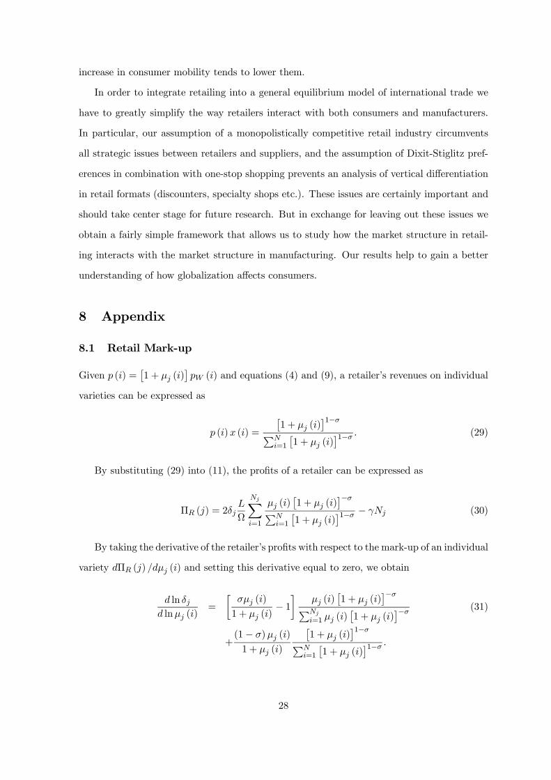
8.1 Retail Mark-up

Given p (i) =£1 + μj (i)

¤pW (i) and equations (4) and (9), a retailer’s revenues on individual

varieties can be expressed as

p (i)x (i) =

£1 + μj (i)

¤1−σPNi=1

£1 + μj (i)

¤1−σ . (29)

By substituting (29) into (11), the profits of a retailer can be expressed as

ΠR (j) = 2δjL

Ω

NjXi=1

μj (i)£1 + μj (i)

¤−σPNi=1

£1 + μj (i)

¤1−σ − γNj (30)

By taking the derivative of the retailer’s profits with respect to the mark-up of an individual

variety dΠR (j) /dμj (i) and setting this derivative equal to zero, we obtain

d ln δjd lnμj (i)

=

∙σμj (i)

1 + μj (i)− 1¸

μj (i)£1 + μj (i)

¤−σPNj

i=1 μj (i)£1 + μj (i)

¤−σ (31)

+(1− σ)μj (i)

1 + μj (i)

£1 + μj (i)

¤1−σPNi=1

£1 + μj (i)

¤1−σ .

28

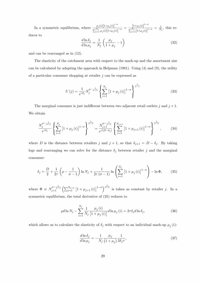
In a symmetric equilibrium, whereμj(i)[1+μj(i)]

−σ

Nji=1 μj(i)[1+μj(i)]

−σ =[1+μj(i)]

1−σ

Nji=1[1+μj(i)]

1−σ =1Nj, this re-

duces tod ln δjd lnμj

=1

Nj

µμj

1 + μj− 1¶

(32)

and can be rearranged as in (12).

The elasticity of the catchment area with respect to the mark-up and the assortment size

can be calculated by adapting the approach in Helpman (1981). Using (4) and (9), the utility

of a particular consumer shopping at retailer j can be expressed as

U (j) =1

eτδjN

ρ− 1σ−1

j

⎧⎨⎩NjXi=1

£1 + μj (i)

¤1−σ⎫⎬⎭1

σ−1

(33)

The marginal consumer is just indifferent between two adjacent retail outlets j and j +1.

We obtain

Nρ− 1

σ−1j

eτδj

⎧⎨⎩NjXi=1

£1 + μj (i)

¤1−σ⎫⎬⎭1

σ−1

=N

ρ− 1σ−1

j+1

eτ(D−δj)

⎧⎨⎩Nj+1Xi=1

£1 + μj+1 (i)

¤1−σ⎫⎬⎭1

σ−1

, (34)

where D is the distance between retailers j and j + 1, so that δj+1 = D − δj . By taking

logs and rearranging we can solve for the distance δj between retailer j and the marginal

consumer:

δj =D

2+1

2τ

µρ− 1

σ − 1

¶lnNj +

1

2τ (σ − 1) ln

⎛⎝ NjXi=1

£1 + μj (i)

¤1−σ⎞⎠− lnΦ, (35)

where Φ ≡ Nρ− 1

σ−1j+1

³PNj+1

i=1

£1 + μj+1 (i)

¤1−σ´ 1σ−1

is taken as constant by retailer j. In a

symmetric equilibrium, the total derivative of (35) reduces to

ρd lnNj −NjXi=1

1

Nj

μj (i)£1 + μj (i)

¤d lnμj (i) = 2τδjd ln δj , (36)

which allows us to calculate the elasticity of δj with respect to an individual mark-up μj (i):

d ln δjd lnμj

= − 1

Nj

μj¡1 + μj

¢ 1

2δjτ, (37)

29

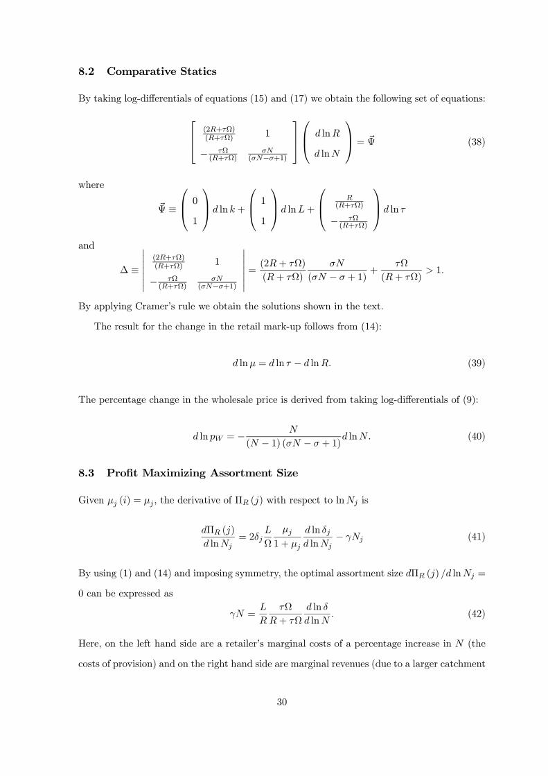
8.2 Comparative Statics

By taking log-differentials of equations (15) and (17) we obtain the following set of equations:

⎡⎢⎣ (2R+τΩ)(R+τΩ) 1

− τΩ(R+τΩ)

σN(σN−σ+1)

⎤⎥⎦⎛⎜⎝ d lnR

d lnN

⎞⎟⎠ = Ψ (38)

where

Ψ ≡

⎛⎜⎝ 0

1

⎞⎟⎠ d ln k +

⎛⎜⎝ 1

1

⎞⎟⎠ d lnL+

⎛⎜⎝ R(R+τΩ)

− τΩ(R+τΩ)

⎞⎟⎠ d ln τ

and

∆ ≡

¯¯ (2R+τΩ)

(R+τΩ) 1

− τΩ(R+τΩ)

σN(σN−σ+1)

¯¯ = (2R+ τΩ)

(R+ τΩ)

σN

(σN − σ + 1)+

τΩ

(R+ τΩ)> 1.

By applying Cramer’s rule we obtain the solutions shown in the text.

The result for the change in the retail mark-up follows from (14):

d lnμ = d ln τ − d lnR. (39)

The percentage change in the wholesale price is derived from taking log-differentials of (9):

d ln pW = − N

(N − 1) (σN − σ + 1)d lnN . (40)

8.3 Profit Maximizing Assortment Size

Given μj (i) = μj , the derivative of ΠR (j) with respect to lnNj is

dΠR (j)

d lnNj= 2δj

L

Ω

μj1 + μj

d ln δjd lnNj

− γNj (41)

By using (1) and (14) and imposing symmetry, the optimal assortment size dΠR (j) /d lnNj =

0 can be expressed as

γN =L

R

τΩ

R+ τΩ

d ln δ

d lnN. (42)

Here, on the left hand side are a retailer’s marginal costs of a percentage increase in N (the

costs of provision) and on the right hand side are marginal revenues (due to a larger catchment

30

area).

The elasticity of the catchment area with respect to the assortment size (d ln δ/d lnN) can

be calculated from (36):d ln δ

d lnN=

ρR

τΩ. (43)

Combining (42) and (43) yields

γN =ρL

R+ τΩ. (44)

Equations (15) and (44) can be solved for the optimal N∗ and R∗.

8.4 Slotting Allowances

A manufacturers profits without slotting allowances are given by ΠM = [pW (i)− β]Q (i)−α

and can be expressed in a symmetric equilibrium as

ΠM =kL

(1 + μ) (σN − σ + 1)− α (45)

If the optimal assortment decision is binding, then these profits are positive when evaluated

at μ∗ and N∗ from (25). This is the case if kL > αhσρ2LγτΩ − (σ − 1) (1 + ρ)

i, or

ρ < ρ ≡ 12

(σ − 1)σ

τΩ

Lγ +

sγτΩk

σα+(σ − 1)

σ

τΩ

Lγ

µ1 +

1

4

(σ − 1)σ

τΩ

Lγ

¶(46)

If condition (46) holds, manufacturing firms are willing to offer slotting allowances in order

to be listed with the retailing firms. These slotting allowances are paid in free goods, so that

a manufacturer agrees to deliver s − 1 units for free in order to get access to the retailing

shelves: ΠM = [pW − β]Q− α− (s− 1)βQ. Profits can then be expressed as

ΠM (s,N, kL, μ, α) =[(1− s) (σ − 1) (N − 1) +N ] kL

[(σ − 1) (N − 1) +N ] (1 + μ)N− α. (47)

These profits are positive when evaluated at N∗ and μ∗ and are decreasing in s. The equi-

librium slotting allowances push profits down to zero, ΠM (s∗, N∗, kL, μ∗, α) = 0, and can be

31

calculated explicitly from (47):

s∗ =

µ1− (1 + ρ)

αN∗

kL

¶σ (N∗ − 1) + 1(σ − 1) (N∗ − 1) (48)

With s∗ the labor market is in equilibrium as well. Because slotting allowances are paid

in goods, they have to be taken into account when calculating labor demand:

N∗

k(α+ βs∗Q) +R∗γN∗ =

N∗px

1 + ρL+

ρ

1 + ρL = L (49)

References

[1] Alonso, William (1964): Location and Land Use, Harvard University Press: Cambridge,

Mass.

[2] Blanchard, Troy; Lyson, Thomas (2002): "Access to Low Cost Groceries in Nonmetropol-

itan Counties: Large Retailers and the Creation of Food Deserts", Measuring Rural

Diversity Conference Proceedings, November 21-22, 2002, Economic Reserach Service,

Washington, D.C., http://srdc.msstate.edu/measuring/blanchard.pdf.

[3] Blanchard, Troy; Lyson, Thomas (2003): Retail Concentration, Food Deserts, and

Food Disadvantaged Communities in Rural America, Final Report for Southern Rural

Development Center-Economic Research Service Food Assistance Grant Program,

http://srdc.msstate.edu/focusareas/health/fa/blanchard02_final.pdf.

[4] Boylaud, Olivier; Nicoletti, Giuseppe (2001): "Regulatory Reform in Retail Distribu-

tion", OECD Economic Studies, 32, 253-274.

[5] Broda, Christian; Weinstein, David E. (2006): "Globalization and the Gains from Vari-

ety", Quarterly Journal of Economics, 121(2), 541-585.

[6] Clarke, Ian (2000): "Retail power, competition and local consumer choice in the UK

grocery sector", European Journal of Marketing, 34(8), 975-1002.

[7] Competition Commission (2000): "Supermarkets. A report on the supply of groceries

from multiple stores in the United Kingdom", Presented to Parliament by the Secretary

32

of State for Trade and Industry by Command of Her Majesty, http://www.Competition-

Commission.org.uk.

[8] Dawson, John (2001): "Strategy and Opportunism in European Retail Internationaliza-

tion", British Journal of Management, 12, 253-266.

[9] Dobson, Paul W.; Clarke, Roger; Davies, Stephen; Waterson, Michael (2001): "Buyer

Power and its Impact on Competition in the Food Retail Distribution Sector of the

European Union", Journal of Industry, Competition and Trade, 1:3, 247-281.

[10] Dobson, Paul W.; Waterson, Michael (1999): "Retailer power: recent developments and

policy implications", Economic Policy, 28, 135-164.

[11] Dobson, Paul W.; Waterson, Michael; Chu, A. (1998): "The welfare consequences of the

exercise of buyer power", Research Paper No. 16, Office of Fair Trading, London.

[12] Dobson, Paul W.; Waterson, Michael; Davies, Stephen W. (2003): "The Patterns and

Implications of Increasing Concentration in European Food Retailing", Journal of Agri-

cultural Economics, 54(1), 111-125

[13] Ellickson, Paul B. (2006): "Quality Competition in Retailing: A Structural Analysis",

International Journal of Industrial Organization, 24 (3), 521-540.

[14] Ellickson, Paul B. (2007): "Does Sutton Apply to Supermarkets?" Rand Journal of

Economics, 38 (1), 43-59.

[15] Federal Trade Commission (2001): "Report on the Federal Trade Commission Work-

shop on Slotting Allowances and Other Marketing Practices in the Grocery Industry",

Washington.

[16] Feenstra, Robert C.; Hanson, Gordon H. (2004): "Intermediaries in Entrepôt Trade:

Hong Kong Re-exports of Chines Goods", Journal of Economics & Management Strategy,

13 (1), 3-35.

[17] Gable, Myron; Topol, Martin T.; Mathis, Stephen; Fisher, Melvyn E. (1995): "Entry

barriers in retailing", Journal of Retailing and Consumer Services, 2 (4), 211-221.

33

[18] Helpman, Elhanan (1981): "International Trade in the Presence of Product Differen-

tiation, Economies of Scale and Monopolistic Competition", Journal of International

Economics, 11, 305-340.

[19] Krugman, Paul R. (1979): "Increasing Returns, monopolistic competition, and interna-

tional trade", Journal of International Economics, 9, 469-480.

[20] Krugman, Paul R. (1980): "Scale Economies, Product Differentiation, and the Pattern

of Trade", American Economic Review, 70, 950-959.

[21] Melitz, Marc J. (2003): "The impact of trade on intra-industry reallocations and aggre-

gate industry productivity", Econometrica, 71, 1695-1725.

[22] Neary, J. Peter (2003): ”Monopolistic Competition and International Trade Theory”, in:

S. Brakman, B.J. Heijdra (eds.): The Monopolistic Competition Revolution in Retrospect,

Cambridge: Cambridge University Press, 159-184.

[23] OECD (2000): "Assessing Barriers to Trade in Services: Retail Trade Services",

TD/TC/WP(99)41, Paris.

[24] Raff, Horst; Schmitt, Nicolas (2005): "Endogenous vertical restraints in international

trade", European Economic Review, 49, 1877-1889.

[25] Raff, Horst; Schmitt, Nicolas (2006): "Exclusive dealing and common agency in interna-

tional markets", Journal of International Economics, 68, 485-503.

[26] Raff, Horst; Schmitt, Nicolas (2007): "Buyer Power in International Trade", Mimeo.

[27] Rauch, James E. (2001): "Business and Social Networks in International Trade", Journal

of Economic Literature, 39, 1177-1203.

[28] Rauch, James E.; Casella, Alessandra (2003): "Overcoming Informational Barriers to

International Resource Allocation: Prices and Ties", The Economic Journal, 113, 21-42.

[29] Richards, Timothy J.; Hamilton, Stephen F. (2006): "Rivalry in Price and Variety among

Supermarket Retailers", American Journal of Agricultural Economics, 88(3), 710-726.

34

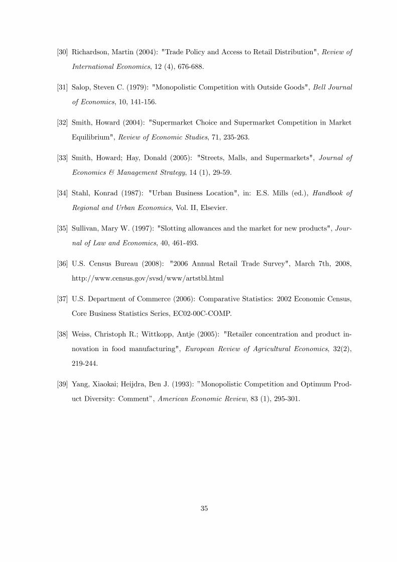
[30] Richardson, Martin (2004): "Trade Policy and Access to Retail Distribution", Review of

International Economics, 12 (4), 676-688.

[31] Salop, Steven C. (1979): "Monopolistic Competition with Outside Goods", Bell Journal

of Economics, 10, 141-156.

[32] Smith, Howard (2004): "Supermarket Choice and Supermarket Competition in Market

Equilibrium", Review of Economic Studies, 71, 235-263.

[33] Smith, Howard; Hay, Donald (2005): "Streets, Malls, and Supermarkets", Journal of

Economics & Management Strategy, 14 (1), 29-59.

[34] Stahl, Konrad (1987): "Urban Business Location", in: E.S. Mills (ed.), Handbook of

Regional and Urban Economics, Vol. II, Elsevier.

[35] Sullivan, Mary W. (1997): "Slotting allowances and the market for new products", Jour-

nal of Law and Economics, 40, 461-493.

[36] U.S. Census Bureau (2008): "2006 Annual Retail Trade Survey", March 7th, 2008,

http://www.census.gov/svsd/www/artstbl.html

[37] U.S. Department of Commerce (2006): Comparative Statistics: 2002 Economic Census,

Core Business Statistics Series, EC02-00C-COMP.

[38] Weiss, Christoph R.; Wittkopp, Antje (2005): "Retailer concentration and product in-

novation in food manufacturing", European Review of Agricultural Economics, 32(2),

219-244.

[39] Yang, Xiaokai; Heijdra, Ben J. (1993): ”Monopolistic Competition and Optimum Prod-

uct Diversity: Comment”, American Economic Review, 83 (1), 295-301.

35

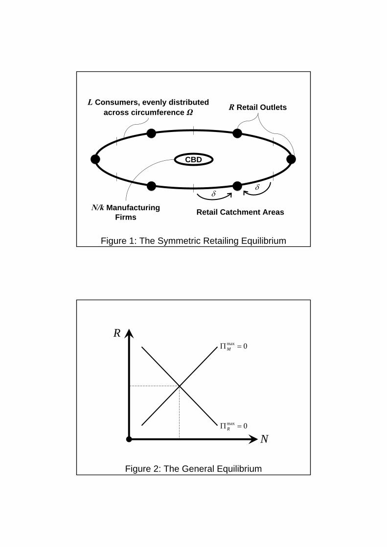
Figure 1: The Symmetric Retailing Equilibrium

L Consumers, evenly distributed across circumference Ω R Retail Outlets

Retail Catchment Areas

CBD

δδ

N/k Manufacturing Firms

Figure 2: The General Equilibrium

R

N0max =ΠR

0max =ΠM

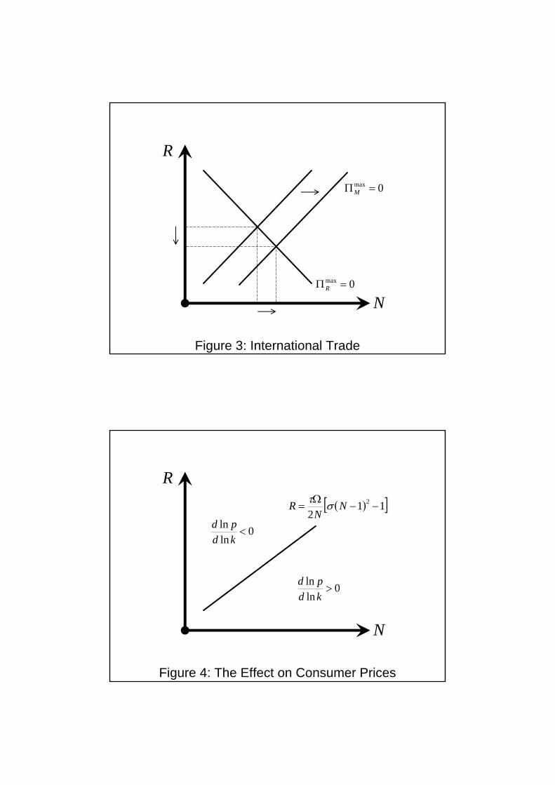
Figure 3: International Trade

R

N

0max =ΠM

0max =ΠR

Figure 4: The Effect on Consumer Prices

R

N

( )[ ]112

2 −−Ω

= NN

R στ

0lnln

<kdpd

0lnln

>kdpd

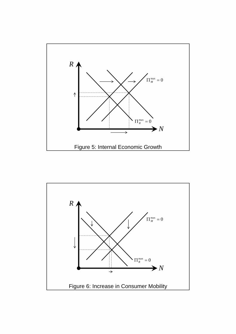
Figure 5: Internal Economic Growth

R

N

0max =ΠM

0max =ΠR

Figure 6: Increase in Consumer Mobility

R

N

0max =ΠM

0max =ΠR

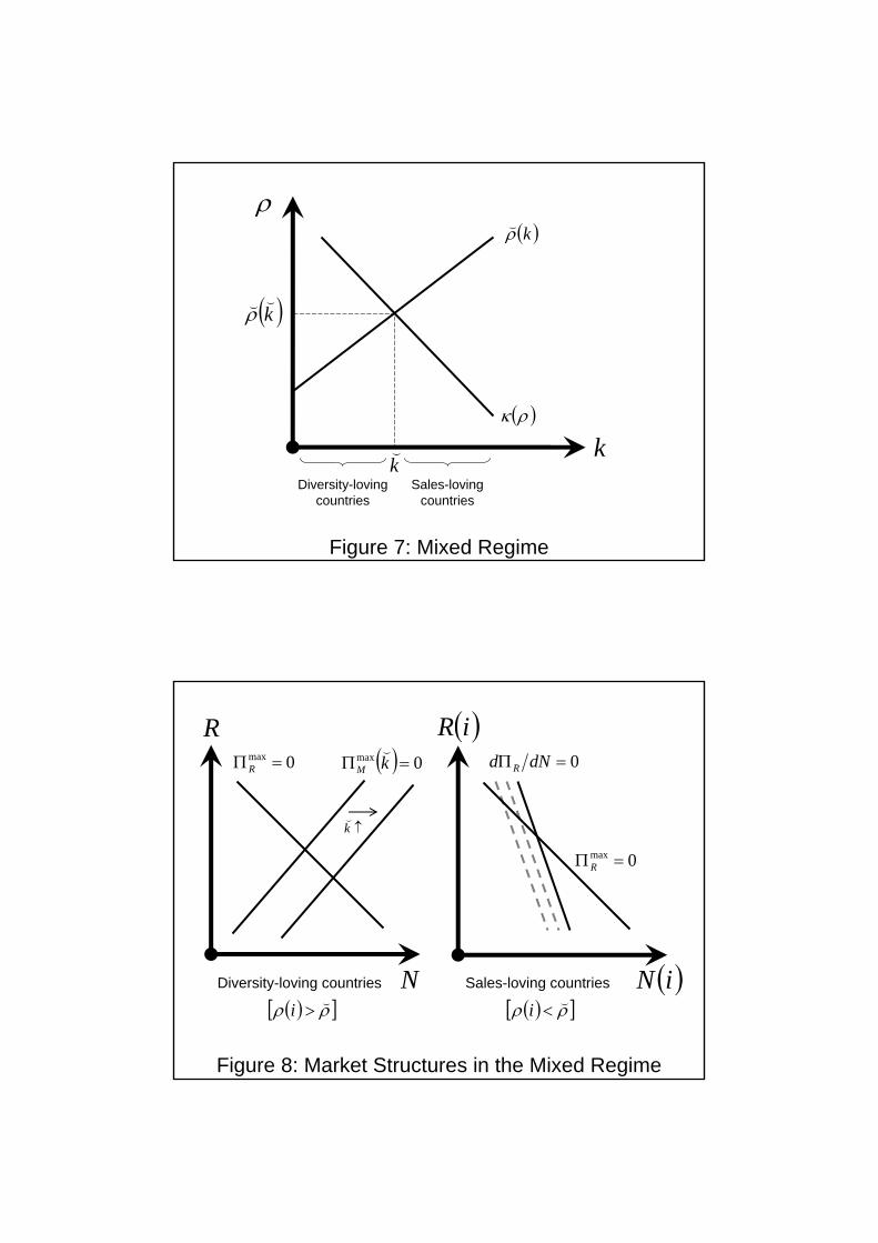
Figure 7: Mixed Regime

ρ

k( )ρκ

( )kρ(

k(

( )k((ρ

Diversity-loving countries

Sales-loving countries

Figure 8: Market Structures in the Mixed Regime

R

N

0max =ΠR ( ) 0max =Π kM

(

( )iN

0max =ΠR

( )iR0=Π dNd R

↑k(

( )[ ]ρρ (>i ( )[ ]ρρ (<iDiversity-loving countries Sales-loving countries

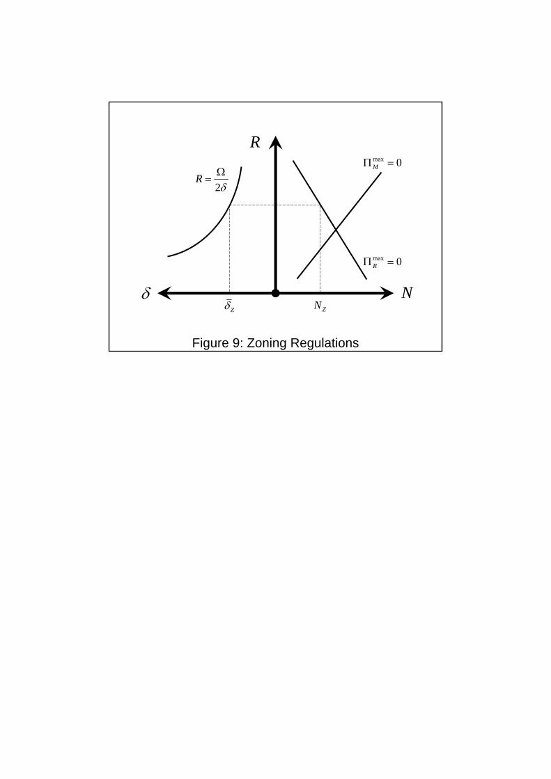
Figure 9: Zoning Regulations

R

N

0max =ΠR

δ2Ω

=R

δZδ ZN

0max =ΠM