Internet of Animals: Foaling detection based on

CONFIDENTIAL UP TO AND INCLUDING 31/12/2029 - DO NOT COPY, DISTRIBUTE OR MAKE PUBLIC IN ANY WAY

accelerometer dataInternet of Animals: Foaling detection based on

Academic year 2019-2020

Master of Science in de informatica

Master's dissertation submitted in order to obtain the academic degree of

Counsellors: Dr. ir. Margot Deruyck, Anniek Eerdekens, Ir. Jaron FontaineSupervisors: Prof. dr. ir. Wout Joseph, Prof. dr. ir. Eli De Poorter

Student number: 01402316Timo De Waele

CONFIDENTIAL UP TO AND INCLUDING 31/12/2029 - DO NOT COPY, DISTRIBUTE OR MAKE PUBLIC IN ANY WAY

accelerometer dataInternet of Animals: Foaling detection based on


Master of Science in de informatica

Master's dissertation submitted in order to obtain the academic degree of

Counsellors: Dr. ir. Margot Deruyck, Anniek Eerdekens, Ir. Jaron FontaineSupervisors: Prof. dr. ir. Wout Joseph, Prof. dr. ir. Eli De Poorter

Student number: 01402316Timo De Waele

Het internet der dieren: veulendetectieaan de hand van accelerometer data

Timo De Waele

Supervisors: Prof. dr. ir. Wout Joseph, Prof. dr. ir. Eli De PoorterCounsellors: Dr. ir. Margot Deruyck, Ir. Anniek Eerdekens, Ir. Jaron

Fontaine

Masterproef voorgelegd voor het behalen van de graad: Master in deInformatica.

Academiejaar 2019-2020

Faculteit WetenschappenUniversiteit Gent

Samenvatting

Er wordt veel mankracht gestoken in het observeren van zwangere merriesom een goed verloop van de bevalling te verzekeren. Automatische obser-vatie van de zwangere merries zou paardeneigenaars kunnen geruststellen.Dit onderzoek stelt een methode voor die veulendetectie kan uitvoeren aande hand van accelerometer data. Een op een autoencoder gebaseerd an-omalie detectie algoritme werd ontwikkeld dat het normale gedrag van demerrie kon onderscheiden van het gedrag dat de merrie vertoonde wanneerde bevalling werd ingezet. Verschillende autoencoder architecturen en an-dere verbeteringen zoals de discrete Fourier transformatie van de acceler-ometer data werden geevalueerd om de performantie van het algoritme teverbeteren. Door een dynamische beslissingsmetriek die zijn beslissing of eenmerrie op het punt staat te bevallen of niet baseerd op bepaalde statistiekenvan elke merrie apart werden veelbelovende resultaten geboekt. Uiteindelijkwerden alle bevalling correct herkend maar voor sommige merries werdenvalse gedetecteerd in de dagen voor de bevalling.

Keywords

Paarden, veulendetectie, gedragdherkenning, machine learning, autoencoder,anomalie detectie, accelerometer

Internet of Animals: Foaling detectionbased on accelerometer data

Timo De Waele

Supervisors: Prof. dr. ir. Wout Joseph, Prof. dr. ir. Eli De PoorterCounsellors: Dr. ir. Margot Deruyck, Ir. Anniek Eerdekens, Ir. Jaron

Fontaine

Master’s dissertation submitted in order to obtain the academic degree ofMaster of Science in de informatica


Faculty of SciencesGhent University

Summary

Lots of effort is put into the monitoring of pregnant mares to ensure a healthydelivery of the foal. Automatic monitoring of the pregnant mares and theirunborn foals could bring horse owners peace of mind. In this research amethod is proposed to perform foaling detection based on accelerometerdata. An autoencoder based anomaly detection algorithm was developedthat could distinguish the mare’s normal behavior from the behavior shownwhen the mare entered labor. Different autoencoder architectures and otherenhancements such as the discrete Fourier transform of the accelerometervalues were evaluated to enhance the performance of the algorithm. By usinga dynamic decision metric that based its decision if a foaling is about to takeplace or not on certain statistics of each mare individually promising resultscould be achieved. In the end all foalings got correctly detected but somemares still showed one or more false alarms in the days before parturition.

Keywords

Equines, foaling detection, behavior detection, machine learning, autoen-coder, anomaly detection, accelerometer

Internet of Animals: Foaling detection based onaccelerometer data

Timo De Waele

Supervisors: Prof. dr. ir. Wout Joseph (promotor), Prof. dr. ir. Eli De Poorter (promotor), Dr. ir. MargotDeruyck, Ir. Anniek Eerdekens, Ir. Jaron Fontaine

Abstract— In this research data acquired from an accelerometer wasused to develop a foaling detection algorithm. The proposed method madeuse of anomaly detection using an autoencoder to detect behaviors that in-dicated the start of labor. Several different configurations and parameterswere evaluated to improve the performance of the algorithm.

Keywords— Equines, foaling detection, behavior detection, machinelearning, autoencoder, anomaly detection, accelerometer

I. INTRODUCTION

With over 16 million horses worldwide, the equine industryresults in 1.6 million full time jobs and a total global revenue ofmore than 270 billion euros [1]. It is clear that a lot of moneyis involved in this growing sector and a major part of it is thebreeding of top sport horses and hence the selling of their spermand embryos, with a single straw of sperm costing up to AC8,000and embryo’s being auctioned off for more than AC50,000 [2][3].Therefore, the breeding of new foals with a good heritage in-cludes financial and emotional involvement of the breeders. Au-tomatic monitoring of pregnant mares and their unborn foals canbring horse owners peace of mind.Many methods to predict the time of parturition already ex-ist, such as looking at the size of the udder and inspecting theamount and character of mammary secretion [4]. Although, thisindication is not exact and is mainly based on intuition builtupon previous experience which makes it a subjective decision.To improve these predictions many different technologies havebeen developed to predict and recognize the time of parturition,such as FoalGuard, Foalert and Birth Alert [5] [6] [7]. But theseall made compromises on either horse comfort, accuracy or easeof use.In this abstract an autoencoder based anomaly detection algo-rithm will be developed that could be deployed for foaling de-tection. Several configurations and parameters of the proposedmodel will be evaluated to improve the performance of algo-rithm.

II. METHODOLOGY

A. Data collection procedure

The data acquisition was done in collaboration with the GhentUniversity clinic of large animal reproduction. During the 2019foaling season 15 mares that were stabled there for observationduring their pre-foaling period were fitted with a triaxial AxivityAX3 accelerometer (Axivity Ltd, Newcastle, United Kingdom).The sensors were attached to the halter in the orientation shownin figure 1. By attaching the device to the halter worn by allmares stabled at the clinic, the impact on the comfort of themare was minimized.

Fig. 1. Direction of each axis in respect to the horse [8]

B. The Datasets

For each dataset the accelerations on all three axes were cap-tured at 50 Hz with a range of -8 g to +8 g. An overview of thesize of the dataset per mare is shown in figure 2. Because of thehigh sampling rate each dataset grows quickly to large propor-tions. To reduce the computational load for handling the amountof data each dataset was reduced to a 1 Hz sampling rate. Thiswas done by taking the average of each group of 50 continu-ous samples. The individual behaviors of each mare were stillidentifiable but the computational load was drastically reduced.

0369121518Days from partus

PirenaAisha

TribelaElektra

ElizeInshallahBrindine

JessElenor

Carraine ZEureka

LadyCassinaTwiggy

Diabolique

Fig. 2. Total time of movement data in days before partus for the participatinghorses.

III. ANOMALY DETECTION MODEL

A. Overview

An autoencoder based anomaly detection algorithm was usedas a basis for the foaling detection system. The main benefit ofthis approach was that it could be trained unsupervised. This

was necessary due to the limited amount of foaling events re-sulting in a heavily unbalanced dataset. The idea behind usingan autoencoder to perform anomaly detection is to train the au-toencoder on regular data only. This makes it overfit on recon-structing regular data making it perform worse on data that sig-nificantly differs from its training set. Because pregnant maresoften show signs of restlessness and symptoms of colic whenthey enter stage one of parturition this idea could be used fordetecting the start of foaling since this behavior is significantlydifferent from the mares normal behavior [9].

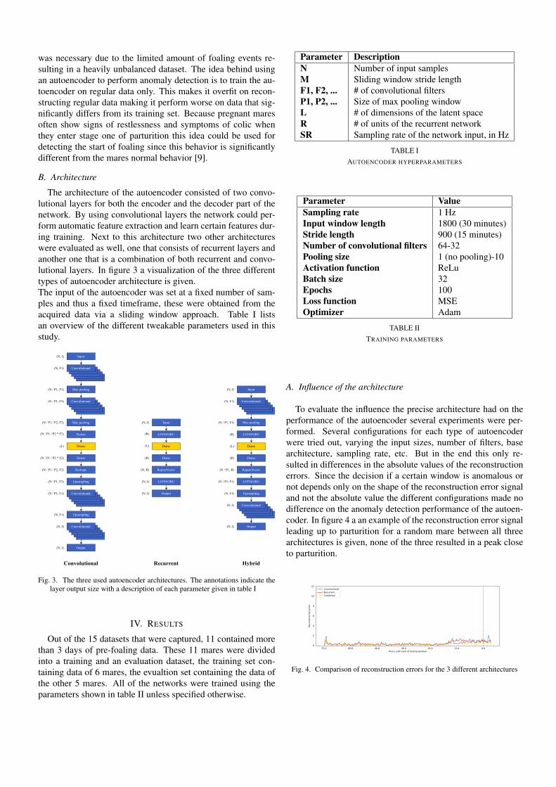
B. Architecture

The architecture of the autoencoder consisted of two convo-lutional layers for both the encoder and the decoder part of thenetwork. By using convolutional layers the network could per-form automatic feature extraction and learn certain features dur-ing training. Next to this architecture two other architectureswere evaluated as well, one that consists of recurrent layers andanother one that is a combination of both recurrent and convo-lutional layers. In figure 3 a visualization of the three differenttypes of autoencoder architecture is given.The input of the autoencoder was set at a fixed number of sam-ples and thus a fixed timeframe, these were obtained from theacquired data via a sliding window approach. Table I listsan overview of the different tweakable parameters used in thisstudy.

Input

Convolutional

(N,I)

(N,F1)

Maxpooling

Dense

Convolutional

Output

Convolutional

Maxpooling

Flatten

Dense

Reshape

Upsampling

Convolutional

Upsampling

(N,I)

(N/P1,F2)

(N/P1,F1)

(N/P1/P2,F2)

(N/P1/P2*F2)

(L)

(N/P1/P2*F2)

(N/P1/P2,F2)

(N/P1,F2)

(N/P1,F1)

(N,F1)

(N,I)

Input(N,I)

Dense

Output

(N,I)

(L)

LSTM/GRU

RepeatVector

LSTM/GRU

Dense

(R)

(R)

(N,R)

(N,I)

Input

Convolutional

(N,I)

(N,F1)

Maxpooling

Dense

Output

Convolutional

Upsampling

(N,I)

(N/P1,F1)

(L)

(N,F1)

(N,I)

LSTM/GRU

Dense

RepeatVector

LSTM/GRU

(R)

(R)

(N/P1,R)

(N/P1,F1)

Convolutional Recurrent Hybrid

Fig. 3. The three used autoencoder architectures. The annotations indicate thelayer output size with a description of each parameter given in table I

IV. RESULTS

Out of the 15 datasets that were captured, 11 contained morethan 3 days of pre-foaling data. These 11 mares were dividedinto a training and an evaluation dataset, the training set con-taining data of 6 mares, the evualtion set containing the data ofthe other 5 mares. All of the networks were trained using theparameters shown in table II unless specified otherwise.

Parameter DescriptionN Number of input samplesM Sliding window stride lengthF1, F2, ... # of convolutional filtersP1, P2, ... Size of max pooling windowL # of dimensions of the latent spaceR # of units of the recurrent networkSR Sampling rate of the network input, in Hz

TABLE IAUTOENCODER HYPERPARAMETERS

Parameter ValueSampling rate 1 HzInput window length 1800 (30 minutes)Stride length 900 (15 minutes)Number of convolutional filters 64-32Pooling size 1 (no pooling)-10Activation function ReLuBatch size 32Epochs 100Loss function MSEOptimizer Adam

TABLE IITRAINING PARAMETERS

A. Influence of the architecture

To evaluate the influence the precise architecture had on theperformance of the autoencoder several experiments were per-formed. Several configurations for each type of autoencoderwere tried out, varying the input sizes, number of filters, basearchitecture, sampling rate, etc. But in the end this only re-sulted in differences in the absolute values of the reconstructionerrors. Since the decision if a certain window is anomalous ornot depends only on the shape of the reconstruction error signaland not the absolute value the different configurations made nodifference on the anomaly detection performance of the autoen-coder. In figure 4 a an example of the reconstruction error signalleading up to parturition for a random mare between all threearchitectures is given, none of the three resulted in a peak closeto parturition.

72.0 60.0 48.0 36.0 24.0 12.0 0.0Hours until start of foaling window

0

2

4

6

8

10

12

Reco

nstru

ctio

n er

ror

ConvolutionalRecurrentCombined

Fig. 4. Comparison of reconstruction errors for the 3 different architectures

B. Method of standardization

One of the most influential parts of the proposed method wasthe way the data was standardized. Two different methods ofstandardization were evaluated. First, data was standardized permare to reduce the influence of halter placement and mare sizeon the network. Second, each input window was standardizedseparately so the autoencoder input has a mean of 0 and a stan-dard deviation of 1. This facilitates the autoencoder ’s learningto reconstruct its inputs.When comparing the two methods, as shown in figure 5, it canbe seen that while standardizing per mare a large peak in the re-construction error appears at parturition. However, when stan-dardizing per input window this peak completely dissappearsand the entire signal is almost completely flat. With standard-ization per input window the near-parturition data and the reg-ular data become completely indistinguishable to the network,standardizing the data per mare is thus necessary to make theproposed algorithm function correctly.


0

2

4

6

8

10

12

Reco

nstru

ctio

n er

ror

Per marePer window

Fig. 5. Comparison of reconstruction errors for both methods of normalization

C. Discrete Fourier transform

By using the acceleration values as input to the autoencoderthe network becomes sensitive to the orientation of the ac-celerometer. The network could get confused if the sensor sud-denly shifts or gets mounted upside down as the baseline ofthe data is now different to what it has seen during training.A way to alleviate the influence is to transform the input win-dows from the time to the frequency domain by applying thediscrete Fourier transform [10]. In the frequency domain thedata becomes much less dependent on the exact orientation ofthe sensor as it now consists of the frequencies that are part ofthe signal and not the absolute acceleration values.In figure 6 an example is presented of the reconstruction errorsfor both accelerometer values as an input and the DFT of thesevalues as an input. The regular model shows no clear peak closeto parturition but the one that makes use of the DFT does. How-ever, to further evaluate the influence of the DFT on the perfor-mance of the proposed method more data is required.

Fig. 6. Reconstruction errors for an autoencoder trained with acceleration val-ues as input (left) and one that was trained with the DFT of the accelerationvalues as its input (right)

D. Other performed experiments

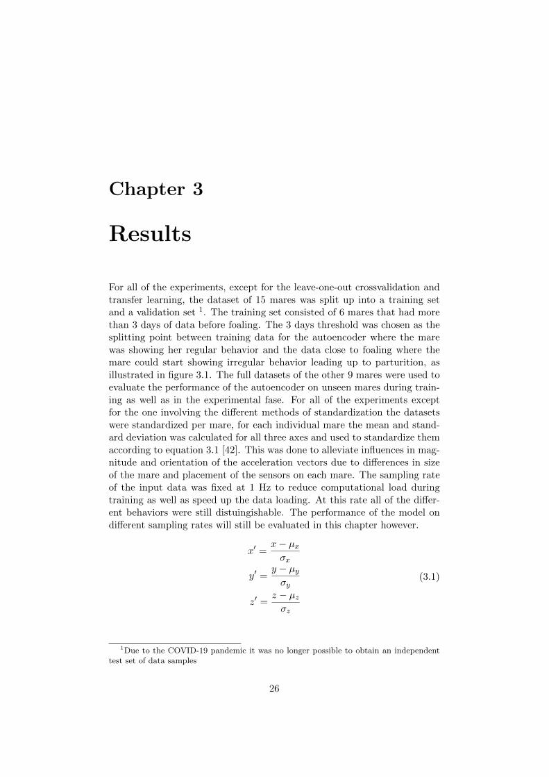
In addition to these three experiments several others were per-formed as well. These include trying out a custom loss functionduring training, applying transfer learning to update the modelwith specific knowledge of each mare, using the latent space ofthe autoencoder to do predictions, etc. All of these experimentsshowed no visible improvement to the reconstruction error sig-nal that was used for anomaly detection.

E. Making a decision

The final step of the anomaly detection algorithm proposed inthis study is making a decision based on the reconstruction er-rors of the autoencoder. This can be done in several ways but themethod proposed is just setting a threshold. If the reconstructionerror for a certain window goes above this set threshold an alarmis triggered. This threshold can be set in many different ways,being either statically were the threshold is the same for eachmare, or dynamically were the threshold is different for eachmare. A dynamically set threshold is preferred as the height ofthe peaks and the baseline of the reconstruction error signal candiffer significantly between mares.To set this threshold each mare should first go trough an analysisphase were the values of the reconstruction errors get analyzedto decide the value of the threshold. In table III the performanceof a number of these thresholds, based on statistics of the recon-struction errors during the analysis phase, are presented. Thebest results in terms of true positives and false positives wereobtained by using a threshold based of the mean plus a fixednumber.Out of the 11 mares, 11 foalings were succesfully recognizedand 7 mares resulted in one or more false alarms in the threedays leading up to parturition. With more data and tweaking ofthe number of standard deviations to add to the mean the lastmethod of deciding a threshold could also prove as succesful.The benefit of adding a number of standard deviations insteadof a fixed value is that it automatically adjusts the threshold tothe variability of the reconstruction error signal of each mare.

Method TP FP FNmax 8 9 3max+ 1 6 5 5mean+ 1 11 7 0mean+ 1.5 10 5 1mean+ 3σ 11 9 0mean+ 5σ 10 7 1

TABLE IIIOVERVIEW OF THE NUMBER OF CORRECT PREDICTIONS/TRUE POSITIVES

(TP), FALSE ALARMS/FALSE POSTIVES (FP) AND UNDETECTED

FOALINGS/FALSE NEGATIVES (FN) FOR A DYNAMICALLY CHOSEN

THRESHOLD

V. CONCLUSION

In this research an algorithm is proposed to detect foalingsfrom accelerometer data based on an anomaly detection modelusing an autoencoder. By training the autoencoder on regular

behavior a metric can be used to decide if a given input is show-ing behavior common to mares entering labor or not based onthe reconstruction error. By making this metric dynamically ad-just to each mare specifically 11 out of the 11 foalings that wereused for evaluation got succesfully detected.Out of these 11 mares there were still some that triggered oneor more false alarms leading up to parturition. Several methodswere proposed and evaluated to reduce the amount of false pos-itives but due to a lack of data no conclusion could be made.Future work should include the acquisition of new datasets tofurther evaluate these proposed improvements. Studies aboutthe influence of different sensor locations on the performance ofthe proposed algorithm should be conducted as well.

REFERENCES

[1] P. Cross, “Global horse statistics internal 02 2019”, Feb.2019.

[2] Jan. 2020. [Online]. Available: https://www.t-online.de/sport/id_75116260/totilas-mitbesitzer-paul-schockemoehle-senkt-preise-fuer-wunderhengst-samen.html.

[3] Jan. 2020. [Online]. Available: https : / / www .flandersfoalauction . be / nl / nieuws /Grand- finale- Flanders- Foal- Auction-sluit-af-met-20108-euro-gemiddeld.

[4] P. M. McCue and R. Ferris, “Parturition, dystocia and foalsurvival: A retrospective study of 1047 births”, EquineVeterinary Journal, no. 44, pp. 22–25, 2012.

[5] 2007. [Online]. Available: http : / / www .foalguard.com.

[6] 2019. [Online]. Available: https://foalert.com.[7] L. A Bate, D. Hurnik, and J. G. Crossley, “Benefits of us-

ing a photoelectric alert system for swine farrowing oper-ations’”, Can. J. Anim. Sci., vol. 71, pp. 909–911, 1991.

[8] [Online]. Available: https://www.premierequine.co.uk/plain-padded-horse-head-collar-c2x21459520.

[9] T. S. Mair et al., Equine Medicine, Surgery and Repro-duction, 2nd edition. Edinburgh: Elsevier, 2013.

[10] A. Roxburgh, “On computing the discrete fourier trans-form”, Dec. 2013.

Lay summary

In this study an algorithm was designed that triggers an alarm when amare was about to give birth. This system made use of data about themovements of the horse. To acquire this data a sensor that could detect thesemovements, called an accelerometer, was attached to the halter the marewas wearing. There were two ways this type of system could be developed,the first is to manually go trough to the data and look for specific signsthat indicate the start of foaling. Then based on the findings of this stepa computer program could be written that would detect these signs andtrigger an alarm. Not only would it be very time consuming to go troughthe data manually as this consisted of many millions of data points, it wouldalso result in an immensely complex computer program as these signs coulddepend on hundres or even thousands of variables. Because developing sucha program would be virtually impossible a second approach was used forthis study, machine learning. In machine learning a computer can, basedon complex mathematical formulas and algorithms, learn to solve complexproblems on its own, without human intervention. The human only needs todefine the space the computer can search trough to look for a solution, afterwhich the computer can train to solve the problem on its own by lettingit look at lots of examples of already solved problems. When this trainingphase is done the computer can be given unsolved problems and solve theseon its own by using the knowledge learned during training.To apply machine learning for developing a foaling detector the idea wasto let the computer learn what regular horse behavior looks like. Once ithad learned this, an input where the mare was showing abnormal behavior,such as rolling, flank watching, etc. when entering labor, would confuse thecomputer would get confused as it doesn’t know anything about this typeof behavior. By measuring this confusion an alarm could be triggered oncethis confusion goes above a certain threshold. Several different methods wereevaluated during this study to improve the capabilities of the computer todistinguish regular from irregulal behavior, such as transforming the dataabout the movements of the mare or using different types of mathematicalformulas to let the computer learn what regular behavior looks like.In the end the computer could correctly detect all of the 11 foalings that itwas given to evaluate the performance. While this may seem as a perfect

result, the proposed approach also resulted in 7 mares giving false alarms,which could lead to alarm fatigue where people don’t take an alarm seriousas it has a high chance of being a false alarm. Because of this future researchshould mainly focus on getting the amount of false alarms as low as possible.

Contents

1 Introduction 11.1 Problem description . . . . . . . . . . . . . . . . . . . . . . . 11.2 Related research . . . . . . . . . . . . . . . . . . . . . . . . . 21.3 Current technology . . . . . . . . . . . . . . . . . . . . . . . . 41.4 Followed approach . . . . . . . . . . . . . . . . . . . . . . . . 7

2 Methodology 82.1 Data . . . . . . . . . . . . . . . . . . . . . . . . . . . . . . . . 8

2.1.1 Procedure . . . . . . . . . . . . . . . . . . . . . . . . . 82.1.2 Data cleaning . . . . . . . . . . . . . . . . . . . . . . . 102.1.3 Data exploration . . . . . . . . . . . . . . . . . . . . . 13

2.2 Model . . . . . . . . . . . . . . . . . . . . . . . . . . . . . . . 162.2.1 Model input data . . . . . . . . . . . . . . . . . . . . . 172.2.2 Model architecture . . . . . . . . . . . . . . . . . . . . 18

2.3 Making a decision . . . . . . . . . . . . . . . . . . . . . . . . 21

3 Results 263.1 Autoencoder architectures . . . . . . . . . . . . . . . . . . . . 28

3.1.1 Convolutional autoencoder . . . . . . . . . . . . . . . 283.1.2 Recurrent autoencoder . . . . . . . . . . . . . . . . . . 293.1.3 Combined autoencoder . . . . . . . . . . . . . . . . . . 30

3.2 Sliding window parameters . . . . . . . . . . . . . . . . . . . 313.3 Sampling rate . . . . . . . . . . . . . . . . . . . . . . . . . . . 333.4 Standardization . . . . . . . . . . . . . . . . . . . . . . . . . . 343.5 Discrete Fourier transform . . . . . . . . . . . . . . . . . . . . 353.6 Custom loss function . . . . . . . . . . . . . . . . . . . . . . . 383.7 Latent representation . . . . . . . . . . . . . . . . . . . . . . . 393.8 Leave-one-out cross-validation . . . . . . . . . . . . . . . . . . 413.9 Transfer learning . . . . . . . . . . . . . . . . . . . . . . . . . 423.10 Filtering . . . . . . . . . . . . . . . . . . . . . . . . . . . . . . 443.11 Decision metric . . . . . . . . . . . . . . . . . . . . . . . . . . 45

3.11.1 Reconstruction errors based threshold . . . . . . . . . 463.11.2 Seasonal-trend composition based threshold . . . . . . 47

4 Discussion 50

5 Conclusion and Future work 53

Chapter 1

Introduction

1.1 Problem description

With over 16 million horses worldwide, the equine industry results in 1.6million full time jobs and a total global revenue of more than 270 billioneuros [1]. It is clear that a lot of money is involved in this growing sectorand a major part of it is the breeding of top sport horses and hence theselling of their sperm and embryos, with a single straw of sperm costing upto AC8,000 and embryo’s being auctioned off for more than AC50,000 [2][3].Therefore, the breeding of new foals with a good heritage includes finan-cial and emotional involvement of the breeders. Automatic monitoring ofpregnant mares and their unborn foals can bring horse owners peace of mind.

More than 10% of pregnant mares suffer from dystocia during foaling, whichcan be recognized by a prolonged or failure of progression of the first orsecond stages of parturation [4][5]. In most of the cases, dystocia occursdue to a malposture of the foal in the uterus or birth canal [6]. This eventrequires early detection to prevent the foal from dying of asphyxiation. Ifstage 2 of the labor takes more than 40 minutes, the percentage of foal mor-tality increases to 20% [4]. The gestation duration of horses can be highlyvariable, ranging from 300 days up to more than 360 days, and is dependenton many factors such as period of insemination, sex of the foal, breed andhereditary factors [7][8]. Therefore, lots of effort goes into the 24/7 monit-oring of pregnant mares. For example, at the Ghent University veterinaryclinic, teams of veterinarians and veterinary medicine students monitor thestabled pregnant mares 24/7 and assist with foalings[9].

By looking at several features of the pregnant mare, like the vulva lax-ity, vulvar discharges, relaxation of the pelvic ligaments, but especially thesize of the udder and the amount and character of mammary secretion, ob-servers can get a strong indication of when the parturation is about to take

1

place [5]. Although, this indication is not exact and is mainly based on in-tuition built upon previous experience which makes it a subjective decision.Therefore, a lot of research, which will be discussed in the next section, isdone in developing automatic foaling detection systems resulting in differenttechnologies.

1.2 Related research

Most research in the field of not only foaling detection but also calving andfarrowing detection is focused on two aspects of the pregnant animal as pre-dictors, namely the temperature and/or the behavior of the animal.

Research has shown that there is a significant decrease in body temper-ature in both mares and cows the day before parturition [10] [11] [12]. Touse this as a predictor for parturition continuous body temperature mon-itoring is required, this can either be done manually by using a rectal ortympanic infrared thermometer or by reading out an implantable microchiptransponder [13]. But this approach is time consuming since human inter-ventions are required for every reading. Using a telemetric gastrointestinalpill could result in more frequent measurements with wireless transmissionto a base station, thus alleviating the need for a human intervention [14].However, by requiring a sensor belt to house the receiving and transmittingequipment, this system imposes a burden on the horse’s comfort, with ex-cessive wear of the surcingle possibly contributing to rubbing on the mare.Because of the drawbacks of both methods, despite body temperature be-ing a good predictor for the detection of foaling, it is hard to implement inpractice.

Another feature that is shown to be useful for the prediction of parturitionis the behavior of the animal. With small activity trackers that incorporatewireless transmission capabilities and extensive battery life becoming moreand more prevalent and affordable, this has the potential to be a practicalapproach for foaling detection. Research has shown that a significant differ-ence in behavior can be observed in the period leading up to to parturitionfor horses but for cows and pigs as well [15] [16] [17] [18] [19]. The differencein behavior is not as well-defined as the change in body temperature andthus further analysis is required to build a predictor out of it. The totallocomotor activity as well as the frequency and total duration of standing,lying, eating and other well-defined behaviors like tail raising, flank watch-ing, urinating et cetera, are found to be useful features in a predictive model.By using these features as input to a machine learning model, researchershave been able to develop a calving detector with good performance [20].An quick summary of the related research is given in table 1.1.

2

Based on this and other research, some foaling detectors have been putinto production and are used in the field today. A short overview of someof these systems will be given in the next section.

Study Animal Features

Body temperature and behaviour ofmares during the last two weeks of preg-nancy (Shaw et al., 1988)

Horse Body temperature,frequency of shownbehaviors

Body temperature fluctuations in theperiparturient horse mare (Cross et al.,1992 )

Horse Body temperature

Methods and on-farm devices to predictcalving time in cattle (Saint-Dizier &Chastant-Maillard, 2015)

Cow Body temperature,tail raising, lyingbouts, clinicalsigns

Detection of the time of foaling by ac-celerometer technique in horses (Equuscaballus)—a pilot study (Aurich et al.,2018)

Horse Increase in activity

Monitoring of total locomotor activity inmares during the prepartum and post-partum period (Bazzano et al., 2015)

Mare Increase in activity

Predicting farrowing based on accelero-meter data (Hietaoja et al., 2013)

Pig Increase in activity

Predicting farrowing of sows housed incrates and pens using accelerometers andCUSUM charts (Hietaoja et al., 2016)

Pig Increase in activity

Prediction of parturition in Holstein dairycattle using electronic data loggers (Bas etal., 2015)

Cow Number of steps,lying bouts, ly-ing time, standingtime

Machine-learning-based calving predic-tion from activity, lying, and ruminatingbehaviors in dairy cattle (Bewley et al.,2017)

Cow Number of steps,lying bouts, ly-ing time, standingtime

Internet of Animals: Foaling detectionbased on accelerometer data (De Waele,2020)

Horse Acceleration val-ues of the mare’shead

Table 1.1: Overview of related research

3

1.3 Current technology

The different foaling alert systems can be broadly categorized into 3 differentcategories, namely systems that work by using sensors placed externally onthe mare, systems that use a device in or around the vagina/vulva of themare and external monitoring tools.

External sensor based systems

Several foaling detection systems work by using accelerometers and/or agyroscopes to determine if the mare is in a lateral recumbent position. Themain benefits of these systems are the fact that no surgical intervention isrequired for placement and usage is not limited to stabled mares. Drawbacksare that they are prone to false positives, e.g. if the mare uses a lateral re-cumbent position to rest or sleep, that could lead to alarm fatigue, as wellas false negatives during dystocia in the initial parturition phase or whenthe mare is not laterally recumbent during foaling.

Two examples of this type of system are FoalGuard and Birth Alarm, Foal-Guard, depicted in figure 1.1, works by using an accelerometer attached tothe halter to determine the position of the mare which, because of the smallform factor, only has a small negative impact on the comfort of the mare[21][22]. Birth Alarm, shown in figure 1.2, uses a gyroscope attached to asurcingle, it manages to obtain a lower occurence of false alarms by waiting acouple of minutes to see if the mare stays down to filter out occurences wherethe mare is sleeping. This results in a delayed alarm trigger but reduces thenumber of false positives and thus the risk of alarm fatigue. However, byattaching the gyroscope on top of the surcingle and thereby restricting themare’s freedom to roll over it, the horse’s comfort is penalized.

Safemate Foalalarm, shown in figure 1.3, implements a different approachby using a sensor that senses perspiration to detect the start of foaling, thiscould however lead to false positives on warm days [23].

Internally placed systems

The Foalert system, shown in figure 1.4, uses two magnets that get suturedto either side of the mares vulva. The alarm gets triggered when the twomagnets separate by the foal being pushed out of the mare, the alarm getstriggered [27]. The false positive rate is low because of the physical inter-action of the foal being required to trigger the alarm, but this also has anegative effect on the number of false negatives in the case of dystocia inthe early stages of parturation. Surturation requires veterinary assistanceto mount and uninstall the device and also adversely affects the wearing

4

Figure 1.1: FoalGuard [24]

Figure 1.2: Birth Alarm [25]

Figure 1.3: Safemate Foalalarm [26]

comfort of the mare.

Another type of foaling detection system in this category is Birth Alert,

5

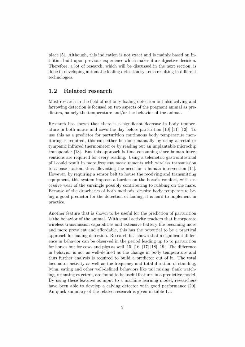
Figure 1.4: Foalert [29]

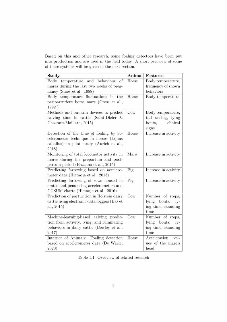
displayed in figure 1.5 [28]. This system consists of 2 parts, a light sensitivesensor, which gets placed inside of the mares vagina, and a microphone, oncethe light sensor gets pushed out of the vagina and starts detecting light againit will make a distinctive sound, that when detected by the microphone willresult in an alarm. No veterinary assistance is required for installation, butit is prone to false positives when the sensor falls out on its own and it doessuffer from the same false negative rate in case of dystocia as Foalert.

Figure 1.5: Birth Alert [30]

External monitoring tools

The last category of tools function without any placement of sensors onthe mare but by using external cameras or microphones, and therefore theydo not impede the comfort of the mare. The EquiView360 uses a cameraplaced in the stable and implements machine vision algorithms to track thebehavior of the horse [31]. While it is primarily used for colic detection, it

6

could be modified for foaling detection use, but this is not yet tested.

Figure 1.6: EquiView360 [32]

1.4 Followed approach

The goal for this thesis is to research the possibility to implement a foal-ing detection system based on accelerometer data that performs equally asgood or better on both comfort and accuracy than current technologies. Toachieve this, small accelerometers attached to the mare will be used to col-lect data about the behavior of the pregnant mare. This data will be passedtrough our foaling detection machine learning algorithm that will trigger analarm if a foaling is about to occur.

In this study, the anomaly detection subfield of machine learning will beexplored for approximating the time of the partus. The rest of this thesisis organised as follows. In chapter 2 a description will be given of the dataacquisition method and the followed approach for the exploring and clean-ing of data, after which the proposed machine learning algorithm to tacklethe problem will be further explained. Chapter 3 lists the conducted exper-iments and the obtained results. In chapter 4 these results will be furtherdiscussed and finally a conclusion will be drawn in chapter 5.

7

Chapter 2

Methodology

2.1 Data

For this study data from 15 expecting mares stabled at the Ghent Universityclinic of large animal reproduction was collected, from May 2019 to August2019. The length of each dataset ranges from three hours to over two weeksprepartus. A complete overview of the size of the dataset per mare is givenin figure 2.1. Out of these 15 mares, 13 entered labor between 10PM and6AM, the other 2 gave birth around noon. One of these mares, Tribela, gavebirth to a twin of foals, a rare occurence [33].

2.1.1 Procedure

The Axivity AX3 triaxial accelerometers (Axivity Ltd, Newcastle, UnitedKingdom), depicted in figure 2.2, were used for data collection. These werechosen for their compact size, broad range of configurability, robustness andextensive battery life. A full overview of the specs is given in table 2.1.

At the start of the measurements, each mare was equipped with two sensors,one placed on top of the withers on a surcingle and one attached on top ofthe halter, as shown in figure 2.3. There were however some issues with thesensor on surcingle. First it would slide down when the mare was activeresulting in the sensor changing location which made it hard to use thisdata in practice. Another, more severe issue, was that due to the sliding thesurcingle would rub against the mares withers and induce rubbing wounds,therefore it was chosen to not use the surcingle for data collection as thewelfare of the mare was of the uttermost importance during this study.

The sensor on top of the halter was attached with ducttape to fix it firmly inplace, after which a couple layers of cohesive bandage was wrapped around itto make sure no ducttape was rubbing against the mares head. The sensorswere placed in the same orientation each time, with the logo facing down

8

0369121518Days from partus

PirenaAisha

TribelaElektra

ElizeInshallahBrindine

JessElenor

Carraine ZEureka

LadyCassinaTwiggy

Diabolique

Figure 2.1: Total time of movement data in days before partus for theparticipating horses.

Figure 2.2: Axivity AX3 Triaxial Accelerometer [34]

and the USB port pointing to the right side of the mare, resulting in theaxis orientation that is shown in figure 2.4. For one mare the sensor wasplaced upside down for some days but this was later fixed during the datacleaning step by flipping the x and z axis. Total time of movement data indays before partus for the participating horses. As for the recording para-meters, a measurement range between -8 g and 8 g was used with a samplingfrequency of 50 Hz as it gave a wide range of resampling possibilities while

9

still having ample battery life.

If the sensor was mounted, it remained on the mare for at least two daysbefore being removed for downloading the data and checking whether itstill worked correctly. For example, one sensor stopped recording after afew hours due to a defective battery, but this was during the first record-ing period so only two days of data were lost. The timestamps of the gapscreated by removing the sensor were stored in a text file so that they couldbe fixed during the data preprocessing phase. Six stables at the veterinaryclinic were equipped with CCTV cameras, the videos from these were down-loaded and used for analyzing behavior leading up to the partus as well asto check for anomalies such as a removed halter, so a gap in the data couldbe recorded.

The raw data for each continuous dataset was then saved to a csv file,containing per sample the timestamp and the x, y and z acceleration values.Alongside this raw data a metadata file was stored per horse containing thename of the mare, the timestamps of when each recording was started andstopped and the moment the amniotic sac burst according to the observingstudents.

Figure 2.3: Placement of the accelerometers

2.1.2 Data cleaning

The first step of the data cleaning process was to trim each dataset to onlycontain the data of when the sensor was attached to the mare. This was

10

Figure 2.4: Direction of each axis in respect to the horse [35]

Parameter Value

Dimensions 23 x 32.5 x 7.6 mmWeight 11gMoisture ingress IPx8 1.5m for 1hrDust ingress IP6xMemory 512 MB Flash non-volatileAcceleration Sample Rate 12.5 - 3200Hz ConfigurableBattery Life 30 days @ 12.5Hz, 14 days @ 100HzAccuracy Range ± 2/4/8/16g ConfigurableAccuracy Resolution upto 13 bit

Table 2.1: Axivity AX3 Triaxal Accelerometer specifications

done by loading the csv containing the raw data via the python frameworkPandas and only keeping the valid sections by removing the sections werethe sensor was not yet on the mare. The trimmed data was then savedto disk. As a next step, these datasets were concatenated so that a singledataset was obtained for each horse containing all the data, which was thenstored as a csv file. These datasets do contain gaps in the data from whenthe sensor was taken of for checking if it was still functioning correctly andthe intermediate downloading of the data.

11

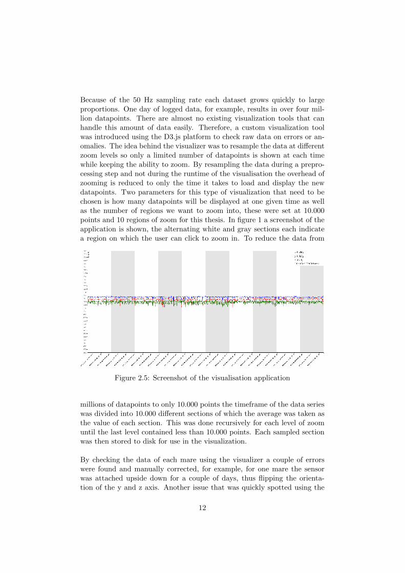
Because of the 50 Hz sampling rate each dataset grows quickly to largeproportions. One day of logged data, for example, results in over four mil-lion datapoints. There are almost no existing visualization tools that canhandle this amount of data easily. Therefore, a custom visualization toolwas introduced using the D3.js platform to check raw data on errors or an-omalies. The idea behind the visualizer was to resample the data at differentzoom levels so only a limited number of datapoints is shown at each timewhile keeping the ability to zoom. By resampling the data during a prepro-cessing step and not during the runtime of the visualisation the overhead ofzooming is reduced to only the time it takes to load and display the newdatapoints. Two parameters for this type of visualization that need to bechosen is how many datapoints will be displayed at one given time as wellas the number of regions we want to zoom into, these were set at 10.000points and 10 regions of zoom for this thesis. In figure 1 a screenshot of theapplication is shown, the alternating white and gray sections each indicatea region on which the user can click to zoom in. To reduce the data from

Figure 2.5: Screenshot of the visualisation application

millions of datapoints to only 10.000 points the timeframe of the data serieswas divided into 10.000 different sections of which the average was taken asthe value of each section. This was done recursively for each level of zoomuntil the last level contained less than 10.000 points. Each sampled sectionwas then stored to disk for use in the visualization.

By checking the data of each mare using the visualizer a couple of errorswere found and manually corrected, for example, for one mare the sensorwas attached upside down for a couple of days, thus flipping the orienta-tion of the y and z axis. Another issue that was quickly spotted using the

12

visualization tool was that for another mare the timezone of the sensor wasset incorrectly, resulting in a 6 hour difference between the actual time of asample and the recorded timestamp, both of these issues had to be fixed upmanually by loading and correcting the relevant dataset.

2.1.3 Data exploration

In this section an overview will be given of some of the most common beha-viors seen in the hour leading up to foaling. First, the data was dowsampledfrom 50 Hz to 1 Hz, at this sampling rate the different behaviors were stilleasily distinguishable but the amount of processing power required to queryand visualize the datasets was drastically reduced. Video footage of the hourbefore foaling was available for 10 out of the 15 mares, this footage was thenused to detect the different types of recurrent behavior shown leading up topartus.

The first noticeable behaviour detected is pacing, i.e. the mare walks rest-lessly in circles in the stable. Figure 2.6 displays the accelerometer patternof this behavior together with normal activity of the same mare for compar-ison. The most notable difference between the data of the normal behaviorversus pacing around is the frequency of the peaks and valleys in the y axissignal, which are much more frequent when the mare is pacing around. Thiscould be attributed to the fact that the mare is walking around and thusaccelerating forward with each step.

Time (minutes)

1

0

1

Acce

lera

tion

(g)

Normal

xyz

0 1 2 3 4 5 6 7 8 9 10Time (minutes)

1

0

1

Acce

lera

tion

(g)

Pacing around

xyz

Figure 2.6: Comparison of normal behaviour vs. pacing around

The second observed behavior is headshaking together with flank watch-ing where the mare would turn her head backwards to watch her side, often

13

combined with shaking her head upwards and/or sideways. This is shown asan accelerometer trace which is compared to normal behavior for the samemare in figure 2.7. The first indicated region is the mare shaking her head,which can be recognized by the high volatility of all three axis. The secondregion indicates flank watching, since for this action the mare needs to tilther head sideways this results in a change of orientation of both the y andz axis.

Time (s)

1

0

Acce

lera

tion

(g)

Normal

xyz

0 20 40 60 80 100 120Time (s)

1

0

1

Acce

lera

tion

(g)

Head shaking

xyz

Figure 2.7: Comparison of normal behaviour vs. head shaking (first region)and flank watching (second region)

Out of the 10 mares for which video footage was available, 9 gave birth whilelying down. Horses have two ways of lying down, being either sternally orlaterally recumbent, in the first case the horse is lying on its sternum withits head still held up, in the latter case the horse is lying completely flat onits side with its head on the ground. In figure 2.8 the accelerometer datafor both of these positions is shown, the darker sections indicate where themare was lying laterally recumbent, the lighter section indicates a sternallyrecumbent position. Lateral recumbency is easily detectable since the z axisbecomes negative as the mare puts her head down, the small peaks in the zvalue can be attributed to the mare lifting her head occasionally. Sternallyrecumbency on the other hand can be recognized by the fact that the valuesof the three axis are more distant from eachother as well as that the x axisnow has the highest positive value and the y axis is now closer to zero. Thesignal while lying down is also less noisy than when the mare was standingupright since the mare mostly takes this position to rest in, thus result-

14

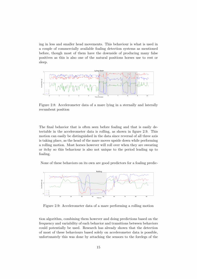
ing in less and smaller head movements. This behaviour is what is used ina couple of commercially available foaling detection systems as mentionedbefore, though most of them have the downside of producing many falsepositives as this is also one of the natural positions horses use to rest orsleep.

0 1 2 3 4 5 6 7 8 9 10Time (minutes)

1

0

1

Acce

lera

tion

(g)

Lying down

xyz

Figure 2.8: Accelerometer data of a mare lying in a sternally and laterallyrecumbent position

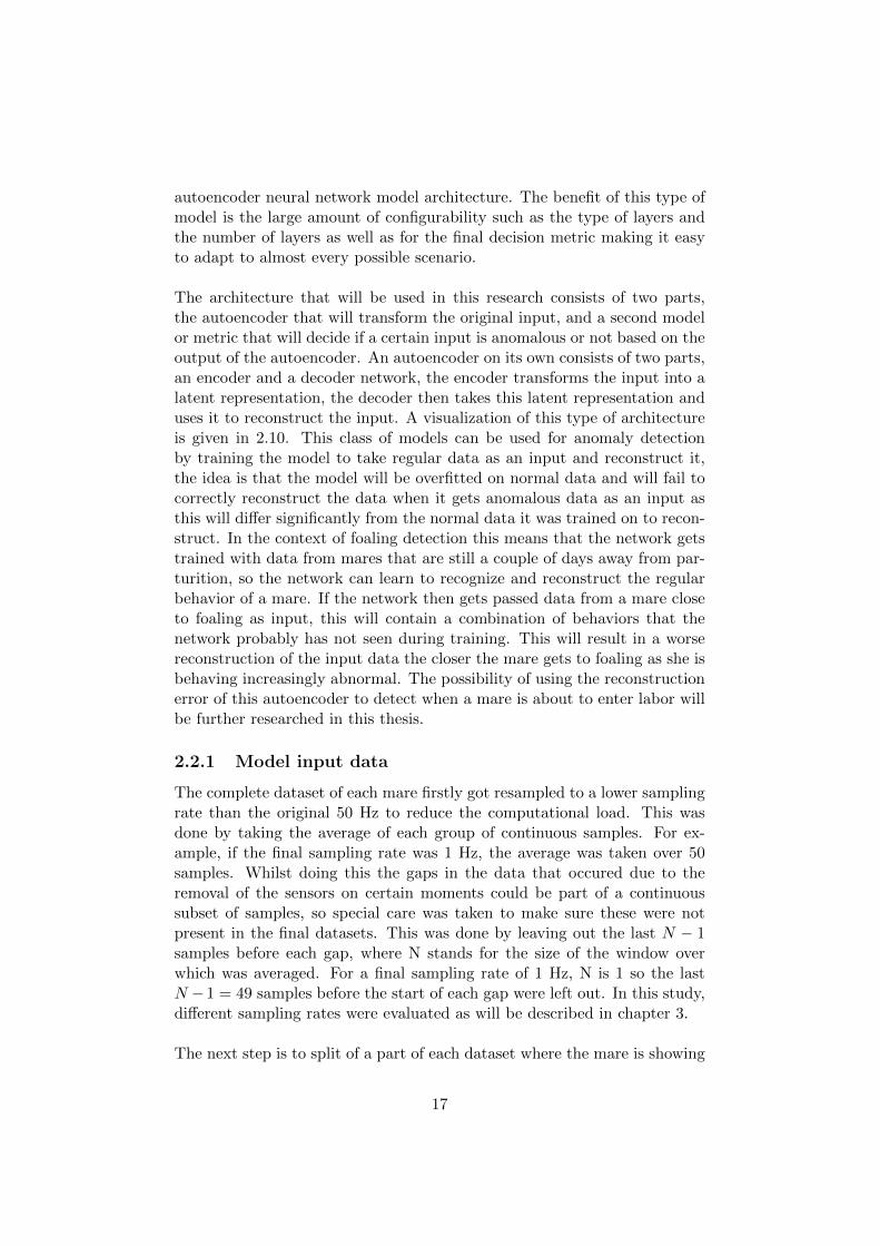
The final behavior that is often seen before foaling and that is easily de-tectable in the accelerometer data is rolling, as shown in figure 2.9. Thismotion can easily be distinguished in the data since reversal of all three axisis taking place, as the head of the mare moves upside down while performinga rolling motion. Most horses however will roll over when they are sweatingor itchy so this behaviour is also not unique to the period leading up tofoaling.

None of these behaviors on its own are good predictors for a foaling predic-

0 10 20 30 40 50 60 70 80 90Time (s)

1

0

1

Acce

lera

tion

(g)

Rolling

xyz

Figure 2.9: Accelerometer data of a mare performing a rolling motion

tion algorithm, combining them however and doing predictions based on thefrequency and variability of each behavior and transitions between behaviorscould potentially be used. Research has already shown that the detectionof most of these behaviours based solely on accelerometer data is possible,unfortunately this was done by attaching the sensors to the forelegs of the

15

mare so the result of this research could not be used directly in this thesis[36]. Due to the lack of video recordings required to label data, the optionof designing an algorithm for detecting the shown behavior was chosen notto further investigate.

2.2 Model

This section will describe the model used to tackle the problem of foalingdetection based on the gathered accelerometer data. In deciding the ap-proach that will be taken for this thesis, two problems had to be taken intoconsideration. First, the lack of video footage, this was only available for10 out of the 15 observed mares and even for the ones that had footage itwas only for a limited amount of time and not the entire period the marewas wearing the accelerometer. Because of this, the chosen approach cannot make use of labeled behaviors since we lack the ground truth data tolabel and train a classifier model for these behaviors. The second issue toconsider was the time we had as an indication for parturition. Studentswatching the mares wrote down the time of amniotic sac rupture, althoughthis was more of a rough approximation than an accurate value since therupture was mostly noticed after it had already happened. Because of thisit would be hard to train a model that was just a classifier or a regressionmodel since we have no precise ground truth to label and train the modelwith, the variability in the time that was noted could result into the modelgetting confused during training, the chosen approach thus had to be ableto handle the uncertainity in its prediction variable. As a result of these twoissues it was opted to go for an anomaly detection approach that was basedon a model that could be trained unsupervised.

The main benefit of an unsupervised anomaly detection model is that itcan be trained entirely without any labeled anomalous instances, which ispreferable in this case since there is a large class inbalance as we only haveone foaling event per mare lasting about 15 minutes but a couple of daysworth of normal data per mare. The idea is to train the model to recognizenormal data after which it could be used to detect samples that are signific-antly different to its training set. Because pregnant mares often show signsof restlessness and symptoms of colic when they enter stage 1 of parturitionthis idea could be used for detecting the start of parturition since this be-havior is significantly different from the mares normal behavior [4]. Thereare several different methods available for performing unsupervised anom-aly detection, such as principal component analysis and isolation forests butfor this thesis it was opted to use a deep learning approach based on an

16

autoencoder neural network model architecture. The benefit of this type ofmodel is the large amount of configurability such as the type of layers andthe number of layers as well as for the final decision metric making it easyto adapt to almost every possible scenario.

The architecture that will be used in this research consists of two parts,the autoencoder that will transform the original input, and a second modelor metric that will decide if a certain input is anomalous or not based on theoutput of the autoencoder. An autoencoder on its own consists of two parts,an encoder and a decoder network, the encoder transforms the input into alatent representation, the decoder then takes this latent representation anduses it to reconstruct the input. A visualization of this type of architectureis given in 2.10. This class of models can be used for anomaly detectionby training the model to take regular data as an input and reconstruct it,the idea is that the model will be overfitted on normal data and will fail tocorrectly reconstruct the data when it gets anomalous data as an input asthis will differ significantly from the normal data it was trained on to recon-struct. In the context of foaling detection this means that the network getstrained with data from mares that are still a couple of days away from par-turition, so the network can learn to recognize and reconstruct the regularbehavior of a mare. If the network then gets passed data from a mare closeto foaling as input, this will contain a combination of behaviors that thenetwork probably has not seen during training. This will result in a worsereconstruction of the input data the closer the mare gets to foaling as she isbehaving increasingly abnormal. The possibility of using the reconstructionerror of this autoencoder to detect when a mare is about to enter labor willbe further researched in this thesis.

2.2.1 Model input data

The complete dataset of each mare firstly got resampled to a lower samplingrate than the original 50 Hz to reduce the computational load. This wasdone by taking the average of each group of continuous samples. For ex-ample, if the final sampling rate was 1 Hz, the average was taken over 50samples. Whilst doing this the gaps in the data that occured due to theremoval of the sensors on certain moments could be part of a continuoussubset of samples, so special care was taken to make sure these were notpresent in the final datasets. This was done by leaving out the last N − 1samples before each gap, where N stands for the size of the window overwhich was averaged. For a final sampling rate of 1 Hz, N is 1 so the lastN −1 = 49 samples before the start of each gap were left out. In this study,different sampling rates were evaluated as will be described in chapter 3.

The next step is to split of a part of each dataset where the mare is showing

17

Encoder Decoder

Latentspace

Figure 2.10: Visualization of an autoencoder architecture

regular behavior for use during training of the autoencoder. The thresholdused for making the decision between regular behavior that will be used fortraining and non training data is also a hyperparameter that will be ex-plained further on in this thesis.

The final step in transforming the datasets into input for the autoencoderwas dividing each dataset into different smaller input subsets of equal lengthcorresponding to the input size of the network. To do this the sliding windowmethod was used where a subset of length N is taken followed by sliding the”window” forward by M steps, this is illustrated in figure 2.11. The choicefor using a sliding window approach instead of just dividing the dataset inequally sized parts without stride was made so that every captured beha-vior was fully contained into at least one of the subsets. Otherwise a certainbehavior could be partly in one subset and partly in the following subset sothat no input subset contained the full behavior. The two parameters i.e.,the length of the window and the stride length are again hyperparametersthan can and will be changed during experiments.

2.2.2 Model architecture

There are many different types of autoencoder architectures, such as sparseautoencoders, contractive autoencoders and variational autoencoders, how-ever for this thesis a regular autoencoder will be developed. The generalshape of an autoencoder is one of an hourglass, where the in- and output

18

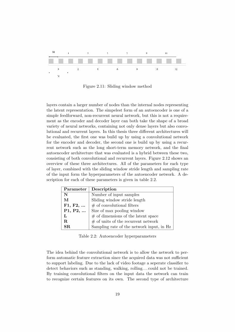
Figure 2.11: Sliding window method

layers contain a larger number of nodes than the internal nodes representingthe latent representation. The simpelest form of an autoencoder is one of asimple feedforward, non-recurrent neural network, but this is not a require-ment as the encoder and decoder layer can both take the shape of a broadvariety of neural networks, containing not only dense layers but also convo-lutional and recurrent layers. In this thesis three different architectures willbe evaluated, the first one was build up by using a convolutional networkfor the encoder and decoder, the second one is build up by using a recur-rent network such as the long short-term memory network, and the finalautoencoder architecture that was evaluated is a hybrid between these two,consisting of both convolutional and recurrent layers. Figure 2.12 shows anoverview of these three architectures. All of the parameters for each typeof layer, combined with the sliding window stride length and sampling rateof the input form the hyperparameters of the autoencoder network. A de-scription for each of these parameters is given in table 2.2.

Parameter Description

N Number of input samplesM Sliding window stride lengthF1, F2, ... # of convolutional filtersP1, P2, ... Size of max pooling windowL # of dimensions of the latent spaceR # of units of the recurrent networkSR Sampling rate of the network input, in Hz

Table 2.2: Autoencoder hyperparameters

The idea behind the convolutional network is to allow the network to per-form automatic feature extraction since the acquired data was not sufficientto support labeling. Due to the lack of video footage a seperate classifier todetect behaviors such as standing, walking, rolling. . . could not be trained.By training convolutional filters on the input data the network can trainto recognize certain features on its own. The second type of architecture

19

Input

Convolutional

(N,I)

(N,F1)

Maxpooling

Dense

Convolutional

Output

Convolutional

Maxpooling

Flatten

Dense

Reshape

Upsampling

Convolutional

Upsampling

(N,I)

(N/P1,F2)

(N/P1,F1)

(N/P1/P2,F2)

(N/P1/P2*F2)

(L)

(N/P1/P2*F2)

(N/P1/P2,F2)

(N/P1,F2)

(N/P1,F1)

(N,F1)

(N,I)

Input(N,I)

Dense

Output

(N,I)

(L)

LSTM/GRU

RepeatVector

LSTM/GRU

Dense

(R)

(R)

(N,R)

(N,I)

Input

Convolutional

(N,I)

(N,F1)

Maxpooling

Dense

Output

Convolutional

Upsampling

(N,I)

(N/P1,F1)

(L)

(N,F1)

(N,I)

LSTM/GRU

Dense

RepeatVector

LSTM/GRU

(R)

(R)

(N/P1,R)

(N/P1,F1)

Convolutional Recurrent Hybrid

Figure 2.12: The three used autoencoder architectures. The annotationsindicate the layer output size with a description of each parameter given intable 2.2

makes use of recurrent network layers instead of convolutional layers. Inthis thesis two types of recurrent layers were used and compared againsteachother i.e., the long short-term memory network and the gated recurrentunit network [37] [38]. Recurrent networks have shown outstanding per-formance in everything that has to do with sequences of data, being textualor time series [39]. The core concept behind these two network types is theimplementation of a memory state inside of the network. When feeding asequence through the network, certain parts of the sequence can be recalledor forgotten and this memory eventually becomes the output of the network.The thought behind using this for modelling the behavior of the mare is thatthe network can keep track of certain behavioral aspects to use these for rep-resenting the entire sequence in the latent space. Since a recurrent networktakes sequences as an input, a layer that repeats its input data a certainnumber of times was needed in the decoder to go from the scalar represent-

20

ation of the latent space back to a sequence of samples. The final approachthat was evaluated was a combined approach with both convolutional andrecurrent layers, first the input gets passed to a convolutional network toperform automatic feature extraction, these self-learned features then getsent to the recurrent network to transform it into a latent embedding.

Once the autoencoders are trained they can be used to perform anomalydetection by obtaining the stream of reconstruction errors for each mare.This is calculated as the mean squared error (MSE) between the input andoutput of the autoencoder, the formula for MSE is given in equation 2.1[40].

MSE =1

N

N∑i=1

(Yi − Yi)2 (2.1)

Where N stands for the number of samples in each window, Y is the originalinput window and Y is the reconstructed input as given by the autoencoder.

This stream of reconstruction errors for each input window to the autoen-coder can then be used to determine if a mare is about foal or not. Themethod of determining this will be explained in further detail in the followingsection.

2.3 Making a decision

An example of a stream of reconstruction errors for a given period and mareis given in figure 2.13. This stream is taken from an input of 100 windowsof each 30 minutes with a stride length of 15 minutes and a sampling rateof 1 Hz. This means that if the first sample window started at 00:00 andended at 00:30 then the second window would start at 00:15 and end at00:45. Based on this stream of reconstruction errors a decision should bemade on when the mare is about to foal, however due to the sliding windowapproach this can only be done based on each window. The precision ofthe prediction is thus dependent on the stride length and sample length ofthe inputs to the autoencoder. For example, if the stride length is set to 15minutes then a prediction can only be made each 15 minutes based on theprevious 30 minutes of data.

The idea is that the stream of reconstruction errors will change when themare is getting closer to foaling, as she will start showing behaviors or com-binations of behaviors the autoencoder does not know how to reconstructas it is unseen and different data, thus increasing the reconstruction error.Based on this difference in reconstruction errors a decision then has to bemade if the mare is close to parturition or not. This can be done in a number

21

75.0 70.0 65.0 60.0 55.0 50.0Hours until start of foaling window

0

2

4

6

8

10

12

Reco

nstru

ctio

n er

ror

Figure 2.13: Example of reconstruction errors

of ways which will be explained in further detail in this section. In figure2.14 an example is given of how the reconstruction errors change leadingup to parturition for a given trained autoencoder. In this chart the lastwindow is the window where foaling occured, the reconstruction error of theautoencoder becomes visibly larger leading up to parturition, it was wellbelow 2 for the entire period but saw a gradual increase from about 2 to 3hours before parturition and had a clear spike in the hour before parturition.For this case setting a fixed threshold that will trigger an alarm once thereconstruction loss goes above it could be a viable approach. The problemwith using this approach is that sometimes the autoencoder will fail on re-constructing its input when the mare is not close to foaling, as shown in2.15. If a single fixed threshold was used in this situation it would result ina false positive. There are two ways of fixing this problem, make the autoen-coder better reconstruct the behaviors shown when the mare is not close tofoaling. In some cases this is not possible however because some mares willshow similar behaviors during a normal situation as when entering labor.This could lead to a false negative and an undetected birth. A second wayof reducing the amount of false positives and false negatives would be to usea different metric of deciding if a mare is about to foal.

One of the other metrics that could be used is using a seasonal-trend decom-position to split the signal of reconstruction errors into its seasonal, trendand residual components [41]. In this decomposition the trend is the globalincreasing or decreasing value of the underlying signal, the seasonal com-ponent is the repeating signal of a given frequency included in the signaland the residual is the noise in the signal that cannot be explained by eitherthe trend or the seasonal component, for the mares a seasonal frequency of24 hours was taken to filter out the moments where the mares were restlessywaiting for food or were being walked by the observers of the veterinaryclinic which was both done at a set time each day. An example of sucha decomposition for the average norm of the acceleration vector over five

22


0

2

4

6

8

10

12

Reco

nstru

ctio

n er

ror

Figure 2.14: Reconstruction errors before foaling


0

2

4

6

8

10

12

Reco

nstru

ctio

n er

ror

Figure 2.15: Reconstruction errors during normal behavior

minute windows of one of the mares is given in figure 2.16.

When this method gets applied to the stream of reconstruction errors aclear jump in the trend becomes visible leading up to parturition for mostmares, an example of this is given in figure 2.17. This does show hope forusing this signal as a predictor for parturition, however this suffers fromthe same drawback as the fixed threshold approach for certain trained au-toencoders, as a jump in the trend of the decomposition could occur whenthe mare was still a couple of hours or days away from parturition, thusagain resulting in false positives, as shown in figure 2.18. This is might besomething that could be worked around with by using some heuristics suchas the angle of the incline and the trend before the incline, some of theseheuristics will be experimented with further on in this thesis.

There are lots of other methods for performing anomaly detection basedon the reconstructions of the autoencoder, such as training a different clas-sifier or regression model on the stream of reconstruction errors or applyinga clustering algorithm to the latent representation, since the representation

23

0 2 4 6 8 10 12 14Days

0.864

0.866

0.868

0.870

0.872

Tren

d

0 2 4 6 8 10 12 14Days

0.010

0.005

0.000

0.005

0.010

0.015

Seas

onal

0 2 4 6 8 10 12 14Days

0.05

0.00

0.05

0.10

0.15

Resid

ual

Figure 2.16: Example of seasonal-trend decomposition for a certain two weekperiod

of the behaviors close to parturition could be significantly different to theones far away from parturition. These methods however will not be studiedfurther in detail for this thesis. In the following chapter the influence of theseveral hyperparameters of the autoencoders as well as the difference in per-formance for the three types of autoencoder architecture will be evaluated,the threshold and seasonal-trend decomposition metrics will be used duringthese experiments for the evaluation of each approach.

24


0.4

0.8

1.2

Reco

nstru

ctio

n er

ror t

rend

Figure 2.17: Trend of reconstruction errors before foaling


0.4

0.8

1.2

Reco

nstru

ctio

n er

ror t

rend

Figure 2.18: Trend of reconstruction errors during normal behavior

25

Chapter 3

Results

For all of the experiments, except for the leave-one-out crossvalidation andtransfer learning, the dataset of 15 mares was split up into a training setand a validation set 1. The training set consisted of 6 mares that had morethan 3 days of data before foaling. The 3 days threshold was chosen as thesplitting point between training data for the autoencoder where the marewas showing her regular behavior and the data close to foaling where themare could start showing irregular behavior leading up to parturition, asillustrated in figure 3.1. The full datasets of the other 9 mares were used toevaluate the performance of the autoencoder on unseen mares during train-ing as well as in the experimental fase. For all of the experiments exceptfor the one involving the different methods of standardization the datasetswere standardized per mare, for each individual mare the mean and stand-ard deviation was calculated for all three axes and used to standardize themaccording to equation 3.1 [42]. This was done to alleviate influences in mag-nitude and orientation of the acceleration vectors due to differences in sizeof the mare and placement of the sensors on each mare. The sampling rateof the input data was fixed at 1 Hz to reduce computational load duringtraining as well as speed up the data loading. At this rate all of the differ-ent behaviors were still distuingishable. The performance of the model ondifferent sampling rates will still be evaluated in this chapter however.

x′ =x− µxσx

y′ =y − µyσy

z′ =z − µzσz

(3.1)

1Due to the COVID-19 pandemic it was no longer possible to obtain an independenttest set of data samples

26

12345678 0

Training

Daysuntilpartus

Figure 3.1: Section of data intended for training the autoencoder

During the first phase of this thesis the models were trained and evaluatedusing the HPC infrastructure of Ghent University 2. This was equippedwith a cluster containing a number of powerful Intel Xeon CPUs and NvidiaTesla V100 GPUs. However due to the small size of the tested models andthe added steps of transfering data between the HPC cluster and a localmachine to train the models and perform visual analysis it was opted to useGoogle Colab 3 for training and evaluation of the models. Colab is a freeto use platform were users can upload and edit jupyter python notebooksto run on virtual instances hosted by Google equipped with powerful GPUsto speed up the training of neural networks build in Tensorflow, specifica-tions of this platform are given in table 3.1. The choice of programminglanguage and software packages for this thesis were the defaults that theGoogle Colab runtime provided, these were Python 3.6.9 as a programminglanguage together with the Tensorflow 2.2.0 and Keras 2.3.0-tf packages asdeep learning library. All of the models were trained for 100 epochs with theadam optimizer and a starting learning rate of 0.001, mean squared errorwas used as loss function. If the training loss did not decrease during 10epochs, the learning rate was reduced by a factor of 0.2, the kernel sizes forall convolutional layers was set fixed at 30 samples. The batch size was setat 32 input windows, in total there were 4144 training input windows and5178 validation samples. The validation set consisted of 5 mares that had3 days or more of prefoaling data and 4 that contained less than 3 days ofprefoaling data which could thus not be used for training.

CPU 2 vCPU @ 2.2GHz

GPU Nvidia Tesla K80, T4, P100

RAM 13GB

Table 3.1: Google Colab specifications

2https://www.ugent.be/hpc/en3https://colab.research.google.com

27

3.1 Autoencoder architectures

3.1.1 Convolutional autoencoder

The first experiment performed was the influence of the number of convolu-tional layers on the reconstructive capabilities of the autoencoder. Thereforetwo models were compared against eachother, one with only one convolu-tional layer in both the encoder and decoder and one containing two convo-lutional layers in both encoder and decoder. A schematic of both networksis given in figure 3.2. After 100 epochs of training the first network with onlyone convolutional layer converged at a training loss of 0.36 and a validationloss of 0.44, the second network with two convolutional layers converged ata training loss of 0.37 and a validation loss of 0.45. Thus adding an extraconvolutional layer to both the encoder and decoder did not seem to make asignificant difference. This is further confirmed if the stream of reconstruc-tion losses is plotted for a mare that had no clear increase in reconstructionerror close to parturition, there is no clear improvement or difference betweenboth autoencoders as can be seen in figure 3.3.

Input

Convolutional

(1800,3)

(1800,32)

Maxpooling

Dense

Convolutional

Output

Convolutional

Maxpooling

Flatten

Dense

Reshape

Upsampling

Convolutional

Upsampling

(1800,3)

(1800,16)

(1800,32)

(180,16)

(2880)

(32)

(2880)

(180,16)

(1800,16)

(1800,32)

(1800,32)

(1800,3)

Input(1800,3)

Dense

Convolutional

Output

Convolutional

Maxpooling

Flatten

Dense

Reshape

Upsampling

(1800,3)

(1800,16)

(180,16)

(2880)

(32)

(2880)

(180,16)

(1800,16)

(1800,3)

Figure 3.2: One layer autoencoder versus two layer autoencoder

Since the number of layers did not make a significant difference on thereconstruction performance of the autoencoder, the number of filters used

28


0

2

4

6

8

10

12

Reco

nstru

ctio

n er

ror

One layerTwo layers

Figure 3.3: Reconstruction errors of both autoencoders

during convolutions was also evaluated. For this experiment the one layerconvolutional autoencoder was used with three different numbers of filters:16, 32 and 64 filters. The training results are given in table 3.2, there aresome small differences between the losses but these do not affect the overallreconstructive abilities of the autoencoder as can be seen in the reconstruc-tion error signal in figure 3.4.

# of filters Training loss Validation loss

16 0.36 0.4432 0.36 0.4664 0.35 0.46

Table 3.2: Training results for different numbers of filters


0

2

4

6

8

10

12

Reco

nstru

ctio

n er

ror

16 filters32 filters64 filters

Figure 3.4: Comparison of reconstruction errors for all 3 configurations

3.1.2 Recurrent autoencoder

For the recurrent autoencoder four different configurations were evaluated.Both the influence of the number of recurrent features and the type of re-

29

current layer on the autoencoders performance was evaluated. The twolayer types being the long short-term memory layer (LSTM) and the gatedrecurrent unit layer (GRU). The main difference between these two layersis that the LSTM has the output gate separate to its hidden state gate,whilst for the GRU, the hidden state is the same as its output gate. Thisreduces the amount of connections in the layer, making it potentially fasterto train than an LSTM while keeping similar performance [43]. Due to theincreased amount of time per epoch to train a recurrent network these net-works were only trained for 50 instead of 100 epochs. Training results forall four configurations can be found in table 3.3. This shows that the gatedrecurrent unit scores slightly better for reconstructing its input. Addingmore recurrent features also has a positive effect on the reconstruction lossof the autoencoder as the network can remember more information fromthe past. For the LSTM this does however inflict a penalty on the trainingtime of the network. For the gated recurrent unit doubling the amount offeatures in its hidden state does not influence its training time significantly.This can probably be attributed to differences in implementation betweenthe two layers. Figure 3.5 shows the plotted reconstruction error signal fora mare that does not have a clear increase in loss when nearing parturition.No useful difference, in terms of foaling prediction capabilities, between thefour implementations can be seen, as the only difference is a higher averagereconstruction error for the LSTM with 32 hidden features as this one scoredsignificantly lower after training. There is also no significant difference in thegeneral shape of the reconstruction error signal between the recurrent andthe convolutional autoencoder, both will show similar performance whenbeing used for foaling prediction.

Type # of features Training loss Validation loss s/epoch

LSTM 32 0.84 0.85 18sLSTM 64 0.72 0.69 21s

GRU 32 0.70 0.68 20sGRU 64 0.69 0.67 20s

Table 3.3: Training results for the recurrent autoencoder

3.1.3 Combined autoencoder

The final autoencoder architecture evaluated in this thesis is a combinedapproach with both a convolutional and a recurrent layer. The first layer ofthis autencoder is a convolutional layer to perform automatic feature extrac-tion. This gets followed by a max pooling layer to reduce the input alongthe time axis and only keep the most relevant extracted features of the inputsequence. Finally it gets passed into the recurrent layer to transform it from

30

Figure 3.5: Comparison of reconstruction errors for all 4 configurations

a time series into the latent space. A combination of the best tested set-tings from previous experiments was used for both layer types. This being16 convolutional filters and a gated recurrent unit with 64 hidden features.Since the size of the input to the recurrent layer was reduced by a factor often due to the max pooling the training time was also reduced to 4 secondsper epoch. Because of this the network was again trained for the full 100epochs. The training resulted in a training loss of 0.50 and a validation lossof 0.51. This was better than a recurrent only architecture but worse thanthe convolutional only model. In figure 3.6 a final comparison between allthree architectures is is given. No architecture managed to create a peakin reconstruction errors before parturition for this mare. The differencesin performance thus can only be attributed to a difference in ability to re-construct the original input. There are no fundamental differences in thereconstruction errors that make one better for foaling prediction than theother. Because of this it was opted to only use the convolutional only au-toencoder in the following experiments due to its significantly faster trainingtime.

3.2 Sliding window parameters

Two of the most important hyperparameters for the predictive model de-veloped in this thesis are the parameters for the sliding window, the sizeand stride length of the window. The stride length affects the number oftraining samples that can be obtained and the frequency at which a pre-diction about the state of the mare can be made. The size of the windowhas the possibility to influence the predictive capabilities of the model. Cer-tain behaviors or sequences of behaviors could only be differentiable by themodel with larger windows or potentially even smaller windows since therewill be less other behaviors to add noise. Three different window sizes andaccording stride lengths will be evaluated in this section, all three were eval-

31


0

2

4

6

8

10

12

Reco

nstru

ctio

n er

ror

ConvolutionalRecurrentCombined

Figure 3.6: Comparison of reconstruction errors for the 3 different architec-tures

Size Stride Training samples Validation samples

15 minutes 7.5 minutes 8313 1038330 minutes 15 minutes 4144 517860 minutes 15 minutes 4110 5144

Table 3.4: Configuration for the sliding window parameters

uated with the two layer convolutional autoencoder architecture with a firstlayer filter count of 32 and a second layer filter count of 16. An overview ofthe tested parameters and respective training and validation dataset sizes isgiven in table 3.4. The training results of this experiment are given in table3.5. The losses get significantly larger when the window size increases asthe network has to compress longer input sequences into the same numberof latent dimensions. In figure 3.7 the reconstruction errors are plotted forone of the mares. Again no significant differences can be seen in the abilitiesof the models to predict foaling. To evaluate the influence of the number oftraining samples on the reconstruction errors of the autoencoder a secondexperiment was done with a fixed window size of 30 minutes and 3 differentstride lengths to vary the amount of training and validation samples. Anoverview of the number of samples per stride length can be found in table3.6, with an overview of the training results given in table 3.7. The resultsin this table show that the validation loss goes down when the stride lengthgoes down, as the network has had more training samples to learn fromand thus could better learn to generalize. In figure 3.7 the reconstructionlosses according to each evaluated stride length are plotted. It is clear thatthe stride length and thus the amount of training samples has no signific-ant influence on the shape of the reconstruction error signal and as a resultthereof it does not improve the false positive or false negative rate. A lowerstride length could still be beneficially since the lower this value is the morefrequent predictions about the state of the mare can be done.

32

Size Training loss Validation loss

15 minutes 0.33 0.3430 minutes 0.36 0.4460 minutes 0.42 0.54

Table 3.5: Training results for different sliding window sizes


0

2

4

6

8

10

12

Reco

nstru

ctio

n er

ror

15 minutes30 minutes60 minutes

Figure 3.7: Comparison of reconstruction errors for 3 different window sizes

Figure 3.8: Comparison of reconstruction errors for 3 different stride lengths

3.3 Sampling rate

To reduce the computational load and data loading times it was opted toresample the data that was captured at 50 Hz down to 1 Hz by taking themean for each group of 50 samples. However, a sampling rate of 5 Hz was

Stride Training samples Validation samples

5 minutes 12416 1552010 minutes 6213 776415 minutes 4144 5178

Table 3.6: Number of samples for a given stride length

33

Stride Training loss Validation loss

5 minutes 0.38 0.4010 minutes 0.37 0.4115 minutes 0.37 0.44

Table 3.7: Training results for 3 different stride lengths

also trained to evaluate the influence of the sampling rate on the predictivecapabilities of the autoencoder. This resulted in a training loss of 0.47 anda validation loss of 0.55. This is significantly higher than the losses for 1Hz, which were 0.37 and 0.44 respectively. This is because the autoencoderhas to encode much more information in the same size latent space. In theplotted reconstruction errors in figure 3.9 a small difference can be seen atabout 10 hours before foaling. At 5 Hz a small peak is visible while for1 Hz this peak is not present. During the period just before foaling nosignificant differences can be seen. For the architecture used in this thesis asampling rate of 1 Hz will thus give similar performance for foaling predictioncompared to higher sampling rates.


0

2

4

6

8

10

12

Reco

nstru

ctio

n er

ror

1 Hz5 Hz

Figure 3.9: Comparison between a 1 Hz and a 5 Hz sampling rate

3.4 Standardization

One of the most influential aspects on the performance of the autoencoderwas which method of standardization was used. The input data was stand-ardized to place the acceleration values of each mare within the same rangeas this could vary widely with the placement of the sensor and the size ofthe mare. For this thesis two different methods of standardization wereused and evaluated, being euther standardizing the data per input windowor standardizing per mare. In figure 3.10 a plot is given of an input windowthat had a low reconstruction error for a network trained with per marenormalization. It can be seen that the differences of the acceleration values

34

between both normalization methods are fairly small in this case. Whenlooked at the same plot but for a window that had a high reconstructionerror the difference in acceleration values between the two becomes muchlarger. Because the data looks so different between the two methods it couldbe that the way of normalizing the data could influence the performance ofthe network. To test this hypothesis the network was trained using bothapproaches, the losses for the network trained with per window normalizeddata were significantly higher at a training loss of 0.64 and a validation lossof 0.73, while per mare normalization was at 0.36 and 0.44. This could beexplained by the fact that the input data is smoothed out when normalizedper window thus making it harder for the network to learn and reconstructspecific behaviors. In figure 3.12 the reconstruction errors signal is plottedfor both methods. When normalized per window almost no difference canbe seen in the signal for the entire three days before foaling. It can be con-cluded that normalizing the data per mare instead of per window is preferedand even necessary for this model to work for foaling prediction.

0 5 10 15 20 25 30Time (minutes)

10.0

7.5

5.0

2.5

0.0

2.5

5.0

7.5

Acce

lera

tion

(g)

xyz

0 5 10 15 20 25 30Time (minutes)

10.0

7.5

5.0

2.5

0.0

2.5

5.0

7.5

Acce

lera

tion

(g)

xyz

Figure 3.10: Comparison between per window normalization (left) and permare normalization (right) for a low reconstruction error window

0 5 10 15 20 25 30Time (minutes)

12.5

10.0

7.5

5.0

2.5

0.0

2.5

5.0

7.5

Acce

lera

tion

(g)

xyz

0 5 10 15 20 25 30Time (minutes)

12.5

10.0

7.5

5.0

2.5

0.0

2.5

5.0

7.5

Acce

lera

tion

(g)

xyz

Figure 3.11: Comparison between per window normalization (left) and permare normalization (right) for a high reconstruction error window

3.5 Discrete Fourier transform

Whilst the model so far shows promising results, with 13 out of the 15 maresshowing a peak in the reconstruction error close to parturition there is still

35


0

2

4

6

8

10

12

Reco

nstru

ctio

n er

ror

Per marePer window

Figure 3.12: Comparison of reconstruction errors for both methods of nor-malization

room for improvement. Of the 15 mares, 10 showed peaks in reconstructionerrors when they were still a few hours or even days away from parturition,which could lead to a large number of false positives. Apart from the highnumber of potential false positives there also were two mares that showedno change in reconstruction errors when the parturition approached. One ofthe approaches tried to improve the performance of the model was to passthe discrete Fourier transformation (DFT) of the input to the autoencoderinstead of the acceleration values. The discrete fourier transformation trans-forms its input from the time domain to the frequency domain [44] i.e., it willshow how strongly each frequency is present in the acceleration signal of themares. To compute this transformation the fast Fourier transform algorithmwas used, implemented in the scientific computing library Numpy [45]. Thistransformation was computed for each input window sampled at 10 Hz. Thishigher sampling rate was necessary as due to the Shannon-Nyquist samplingtheorem [46] the discrete Fourier transform can only transform the input toa range of 0 to half the sampling frequency to the frequency domain.

An example of such a transformation for both the input window containingparturition and a regular window is given in figure 3.13. Only the frequen-cies between 0 and 0.2 Hz are displayed since outside this range there waslittle to no variation. From this visualization it is immediatly clear thatmost of the activity is confined to the lower frequencies between 0 and 0.05Hz. The Fourier transform of the window containing the foaling shows thatthere is a lot more activity and variability in these lower frequency regionswhen the mare is entering labor than during a regular period.

Because of this difference between the result of the transformation on thetwo windows it was chosen to test the model with the Fourier transform ofthe acquired data as its input. This showed promising results, with 15 outof the 15 mares now showing a visible increase in its reconstruction errors

36

when nearing parturition, an increase of 2 mares in comparison to using justthe acceleration values as input. When looking at the number of mares thatshowed a spike in reconstruction errors when still some time away from par-turition there was also an improvement with only 9 out of 15 mares showingsuch a spike compared to the 10 out of 15 for the regular approach. An ex-ample of a mare which had no clear spike before parturition with the regularinput data but that did have an increase in its reconstruction errors whenusing the Fourier transform is given in figure 3.14. Note the difference inthe range of the y-axis, for the Fourier transform the absolute error valueswere significantly smaller in magnitude.

0.000 0.025 0.050 0.075 0.100 0.125 0.150 0.175 0.200Frequency (Hz)

0

50

100

150

200

Mag

nitu

de

x-axis (normal)

0.000 0.025 0.050 0.075 0.100 0.125 0.150 0.175 0.200Frequency (Hz)

0

50

100

150

200

Mag

nitu

de

y-axis (normal)

0.000 0.025 0.050 0.075 0.100 0.125 0.150 0.175 0.200Frequency (Hz)

0

50

100

150

200

Mag

nitu

de

z-axis (normal)

0.000 0.025 0.050 0.075 0.100 0.125 0.150 0.175 0.200Frequency (Hz)

0

50

100

150

200

Mag

nitu

de

x-axis (partus)

0.000 0.025 0.050 0.075 0.100 0.125 0.150 0.175 0.200Frequency (Hz)

0

50

100

150

200

Mag

nitu

de

y-axis (partus)

0.000 0.025 0.050 0.075 0.100 0.125 0.150 0.175 0.200Frequency (Hz)

050

100150200

Mag

nitu

de

z-axis (partus)

Figure 3.13: Example of the discrete Fourier transform for two sample win-dows, the left one containing regular behavior and the right one containingthe behavior shown around foaling

72.0 60.0 48.0 36.0 24.0 12.0 0.0Time (minutes)

0.0

0.25

0.5

0.75

1.0

Reco

nst

ruct

ion e

rror

Discrete Fourier transform

72.0 60.0 48.0 36.0 24.0 12.0 0.0Time (minutes)

0

2

4

6

8

10

12

Reco

nst

ruct

ion e

rror

Regular

Figure 3.14: Reconstruction errors for an autoencoder trained with acceler-ation values as input (left) and one that was trained with the DFT of theacceleration values as its input (right)

37

3.6 Custom loss function

A second idea that was tried out for improving the performance of theautoencoder was implementing a custom loss function. The idea that wasimplemented by the custom loss function is that the reconstruction errorof the autoencoder should be low during regular behavior and high whennearing parturition. To achieve this a weight function was added to the lossfunction of the model during training that would reward the network whenit achieved a higher reconstruction error on the data close to foaling. Thisweight function took the shape of a logistic sigmoid curve that was given byequation 3.2 [47].

w =W + 1

1 + e(−S·(t−T2)−W (3.2)

Where W is the minimum weight value, S is the steepness of the sigmoidcurve, t is the time in minutes until parturition as indicated by the ruptureof the amniotic sac and T is the time before parturition in minutes fromwhere the assigned weight starts to deviate from 1.

To use this during training every training sample that was closer to partur-ition than the value of T was annotated with its time to foaling in minutes.All of the other samples as well as the entire validation dataset were annot-ated with the value of T as its time to foaling feature to keep the input shapeconstant. For this approach the training datasets were not capped at 3 daysbefore partus since the entire dataset is now required during training. Thetraining loss function used for training the autoencoder is given in equation3.3.

loss = w ·MSE (3.3)

Where w is the weight as given in equation 3.2. By capping the annotatedtime until foaling for training samples at T the weight factor function takeson the shape as plotted in figure 3.15.

Because of the reward for a higher reconstruction error close to parturi-tion the network now had the tendency to severly overfit on its trainingdata and just focus on the parts of the data that would reward it. To com-bat this behavior L1 regularization with a regularization factor of 0.01 wasused on all trainable layers. For evaluation the network was trained severaltimes with different combinations of the parameters for the sigmoid weightfunction. In the end the settings used for evaluating the custom loss functionwere the ones that were used in figure 3.15. This custom function resultedin significantly higher reconstruction errors on peaks while the baseline waskept the same as shown in figure 3.16. Since by including the three daysbefore parturition into the training dataset the model now was trained in amore supervised manner. Because of this only the validation dataset will be

38

12 10 8 6 4 2 0Hours until foaling

1.0

0.5

0.0

0.5

1.0W

eigh

t

Figure 3.15: Plot of the weight factor for the custom loss function withT = 360, W = 1.1 and S = 0.05

looked at for evaluation. Out of the 9 mares used for validation 8 showedincreases in the reconstruction errors when nearing parturition. As for peaksthat were not near parturition not much has changed as well, with 5 outof 9 mares showing peaks in reconstruction errors during regular behavior.So while this does not improve the overal performance of the model, it doeshave the potential to achieve better performance by acquiring more data tomake the network learn to better differentiate between near-foaling behaviorand regular behavior.

24.0 18.0 12.0 6.0 0.0Hours until start of foaling window

0.0

10.0

20.0

30.0

40.0

Reco

nstru

ctio

n er

ror

RegularCustom loss

Figure 3.16: Comparison of reconstruction errors between the regular lossfunction (MSE) and a custom implementation favoring higher losses nearparturition

3.7 Latent representation

Until now only the reconstruction error signal was used to assess the per-formance of the autoencoder on the foaling prediction problem. The distri-bution of input windows in the latent space of the autoencoder does however

39

also have the potential to be a good predictor. It could be that the autoen-coder transforms its input into the latent space in such a way that outlierdetection or clustering on these representations could be a good predictorfor parturition.

The first experiment conducted to evaluate this hypothesis was rdone byreducing the number of latent dimensions to just two dimensions. By doingthis the distribution of the latent representations could be inspected visu-ally. But before this could be done the difference between reconstructionbehavior for the network with 32 and 2 latent dimensions had to be eval-uated to make sure that there was no significant penalty for reducing thenumber of dimensions. The training and validation loss of the autoencoderwith two latent dimensions was significantly higher than the one with 32latent dimensions at 0.70 and 0.78 respectively. This was expected sincethe autoencoder had to embed more information in a smaller space. Infigure 3.17 a visual comparison is given between both autoencoders. Bothimplementations show peaks at the same time, albeit higher peaks for thetwo dimensional implementation. It can thus be concluded that reducingthe latent space to only two dimensions will not significantly reduce theperformance of the autoencoder for foaling prediction as this is mainly de-pendent on the shape of the reconstruction error signal and not the absolutevalues.


0

2

4

6

8

10

12

Reco

nstru

ctio

n er

ror

32 latent dimensions2 latent dimensions

Figure 3.17: Comparison of reconstruction errors between an autoencoderwith 2 and one with 32 latent dimensions

In figure 3.18 a scatterplot of the latent representations in these two di-mensions is given as an example. All of the mares showed the same patternwhere the representations for the windows close to foaling are randomly dis-tributed troughout the latent space. This random distribution of the inputwindows in the latent space also occured in a three dimensional latent space.It can thus be concluded that performing a clustering algorithm on the latentspace would not be a viable method of performing foaling detection for an

40

autoencoder approach as there is no noticeable difference between the rep-resentations of windows close to foaling and windows far away from foaling.

0 2 4 6 8 10 12 14

0

2

4

6

8

10

12

14

Partus

0

2

4

>= 6

Hours until start of foaling window

Figure 3.18: Example scatterplot of the latent representations for a randommare

3.8 Leave-one-out cross-validation

For all of the previous experiments in this section a fixed training and val-idation set of 6 and 9 mares respectively was used for each trained model.To proof that the proposed model did not depend on the specific trainingset that was used but could generalize well a Leave-one-out cross-validation(LOOCV) was performed. The first step in the LOOCV experiment was tofilter the original datasets to only contain the mares that had more than 3days of pre-foaling data available because each mare will now be part of atraining dataset and thus had to be cut at the three day before parturitionpoint. In the end 11 out of the 15 mares had more than three days of pre-foaling data and were available for use during LOOCV. For each of these 11mares a seperate autoencoder was trained using the dataset of this mare for

41

validation and the other 10 datasets for training. In figure 3.19 a comparisonbetween the reconstruction errors for a regular trained autoencoder and anLOOCV trained autoencoder is given. For this visualization the data of amare that was part of the training set of the regularly trained autoencoderwas used to see if there was a significant difference in reconstruction errorsif the autoencoder has seen the mare’s behavior during training or not. Byvisually inspecting the difference in reconstruction errors signals for bothmodels it can be observed that there are only small differences in the abso-lute values. The peaks and valleys of the signal are still the same shape andtake place at the same time. This observation can be made for all 11 mares.Because of this it can be concluded that the network sufficiently generalizesand no overfitting to the training data took place.


0

2

4

6

8

Reco

nstru

ctio

n er

ror

LOOCVRegular

Figure 3.19: Comparison of reconstruction errors between regular trainingand leave-one-out cross-validation training

3.9 Transfer learning

While the approach used up this point shows good results in terms of pre-dicting parturition there still were a large number of false positives. Out ofthe 11 mares that had more than three days of pre-parturition data avail-able, 5 showed a clear spike in reconstruction errors in the three days leadingup to parturition but still more than a couple of hours away from partus.This could potentially result in a false positive depending on the metric usedto decide when parturition is about to take place. To try and combat this,transfer learning was tried out and evaluated. This was already an idea toimplement from the start of this research. The idea behind using transferlearning for foaling prediction was to first train a general base model froma dataset of regular behavior from a couple of unspecifified mares. Thiswould allow the autoencoder to learn how to reconstruct general horse be-havior. If the model then got deployed in a real world setting it would firstgo trough a setup phase. During this phase it would continuously apply

42

transfer learning in an online fashion and update its knowdlegde for themare it was observing. After a couple of days of transfer learning the modelshould have learned the intrinsics of the observed mare after which it wouldswitch over to inference mode. Because the model is now better fitted tothis specific mare it could be better in differentiating between regular andabnormal behavior.

To test out this hypothesis in the setting of this research the regular modelwas used as a base model on which, for each of the five validation mares,transfer learning was then applied. First only the data up to three daysbefore parturition of the validation mares was kept for use during training.Once the training data was obtained the weights of base model got loadedfor each of the five mares after which the model got trained for an additional25 epochs on data of a single mare. The result of this experiment for onemare that showed false positives with the regular model is shown in figure3.20. Again there are high peaks in the reconstruction errors visible longbefore parturition is about to take place, transfer learning the entire modeldid not result in a potential lower false positive rate.


0369

121518

Reco

nstru

ctio

n er

ror

Figure 3.20: Example of the reconstruction errors after transfer learning theentire model for an additional 25 epochs

In transfer learning an already trained model it is common practice tofreeze certain layers during the transfer learning phase [48]. In most casesthe earlier layers in the network get frozen for transfer learning, and onlythe later layers actually get updated. This is done because earlier layersmostly extract more general features while later layers are trained to ex-tract more specific features in regards of the training data. In the case ofthe autoencoder used in this thesis it was chosen to freeze the first andlast convolutional layer and leave the other layers unlocked during transferlearning. Doing this however resulted in almost no visible difference whenlooking at the reconstruction errors, as shown in figure 3.21. In both graphsthere is almost no difference between the reconstruction error signals. With

43

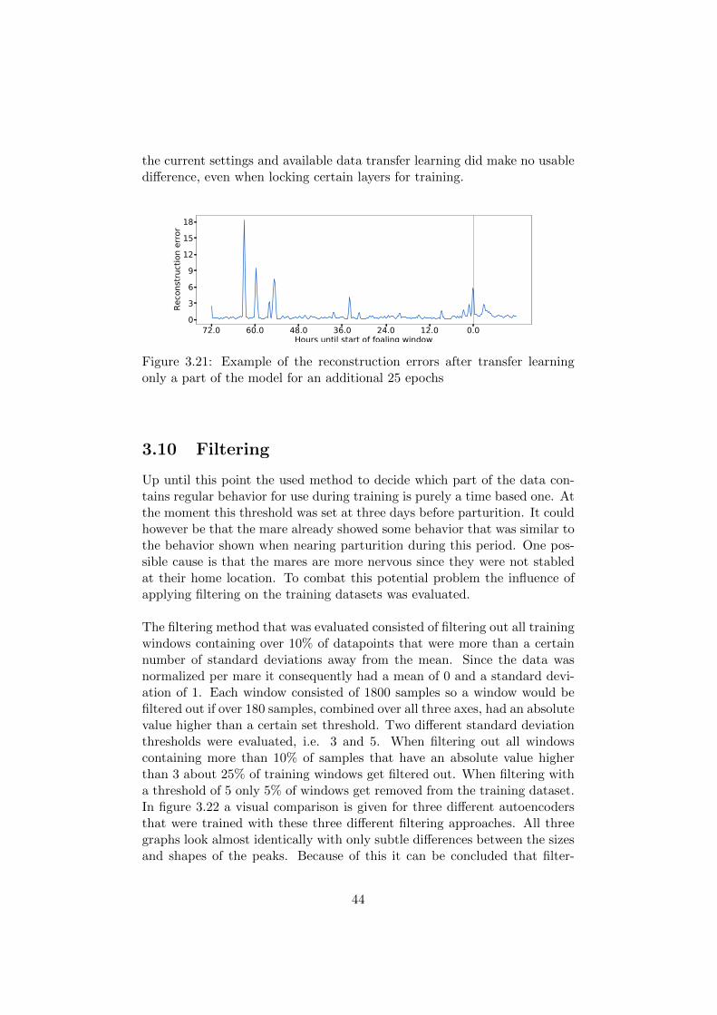
the current settings and available data transfer learning did make no usabledifference, even when locking certain layers for training.


0369

121518

Reco

nstru

ctio

n er

ror

Figure 3.21: Example of the reconstruction errors after transfer learningonly a part of the model for an additional 25 epochs

3.10 Filtering

Up until this point the used method to decide which part of the data con-tains regular behavior for use during training is purely a time based one. Atthe moment this threshold was set at three days before parturition. It couldhowever be that the mare already showed some behavior that was similar tothe behavior shown when nearing parturition during this period. One pos-sible cause is that the mares are more nervous since they were not stabledat their home location. To combat this potential problem the influence ofapplying filtering on the training datasets was evaluated.

The filtering method that was evaluated consisted of filtering out all trainingwindows containing over 10% of datapoints that were more than a certainnumber of standard deviations away from the mean. Since the data wasnormalized per mare it consequently had a mean of 0 and a standard devi-ation of 1. Each window consisted of 1800 samples so a window would befiltered out if over 180 samples, combined over all three axes, had an absolutevalue higher than a certain set threshold. Two different standard deviationthresholds were evaluated, i.e. 3 and 5. When filtering out all windowscontaining more than 10% of samples that have an absolute value higherthan 3 about 25% of training windows get filtered out. When filtering witha threshold of 5 only 5% of windows get removed from the training dataset.In figure 3.22 a visual comparison is given for three different autoencodersthat were trained with these three different filtering approaches. All threegraphs look almost identically with only subtle differences between the sizesand shapes of the peaks. Because of this it can be concluded that filter-

44

ing out windows with high variability during training does not significantlyinfluence the reconstructive power of the proposed method.


0

2

4

6

8

10

12

Reco

nstru

ctio

n er

ror

No filtering


0

2

4

6

8

10

12

Reco

nstru

ctio

n er

ror

3 standard deviations


0

2

4

6

8

10

12

Reco

nstru

ctio

n er

ror

5 standard deviations

Figure 3.22: Comparison of the reconstruction errors between the threedifferent filtering methods

3.11 Decision metric

Lots of different methods to improve the predictive performance of the au-toencoder were evaluated in the previous sections, but the goal of this thesisis to develop a foaling prediction algorithm. To accomplish this a final de-cision metric should be evaluated. This metric will decide, based on thereconstruction errors of the autoencoder, when parturition is about to takeplace. Two different approaches for this metric will be evaluated, decid-ing based on the raw reconstruction errors signal or deciding based on the

45

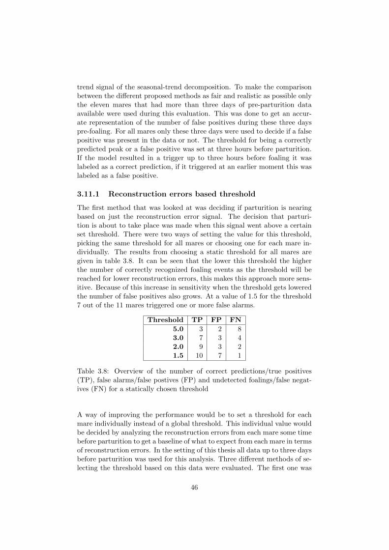
trend signal of the seasonal-trend decomposition. To make the comparisonbetween the different proposed methods as fair and realistic as possible onlythe eleven mares that had more than three days of pre-parturition dataavailable were used during this evaluation. This was done to get an accur-ate representation of the number of false positives during these three dayspre-foaling. For all mares only these three days were used to decide if a falsepositive was present in the data or not. The threshold for being a correctlypredicted peak or a false positive was set at three hours before parturition.If the model resulted in a trigger up to three hours before foaling it waslabeled as a correct prediction, if it triggered at an earlier moment this waslabeled as a false positive.

3.11.1 Reconstruction errors based threshold

The first method that was looked at was deciding if parturition is nearingbased on just the reconstruction error signal. The decision that parturi-tion is about to take place was made when this signal went above a certainset threshold. There were two ways of setting the value for this threshold,picking the same threshold for all mares or choosing one for each mare in-dividually. The results from choosing a static threshold for all mares aregiven in table 3.8. It can be seen that the lower this threshold the higherthe number of correctly recognized foaling events as the threshold will bereached for lower reconstruction errors, this makes this approach more sens-itive. Because of this increase in sensitivity when the threshold gets loweredthe number of false positives also grows. At a value of 1.5 for the threshold7 out of the 11 mares triggered one or more false alarms.

Threshold TP FP FN

5.0 3 2 83.0 7 3 42.0 9 3 21.5 10 7 1

Table 3.8: Overview of the number of correct predictions/true positives(TP), false alarms/false postives (FP) and undetected foalings/false negat-ives (FN) for a statically chosen threshold

A way of improving the performance would be to set a threshold for eachmare individually instead of a global threshold. This individual value wouldbe decided by analyzing the reconstruction errors from each mare some timebefore parturition to get a baseline of what to expect from each mare in termsof reconstruction errors. In the setting of this thesis all data up to three daysbefore parturition was used for this analysis. Three different methods of se-lecting the threshold based on this data were evaluated. The first one was

46

setting the threshold at the maximum value, or maximum plus a fixed value,encountered during the analysis phase. The second one was calculating themean of the reconstruction errors during the analysis phase and setting thethreshold at this mean plus a certain value. Because some mares showed alot more variability in their reconstruction error signal than others the finalmethod that was evaluated was again taking the mean but now adding anumber of standard deviations to it to set the threshold. Making the addedvalue depend on the standard deviation of each mare should account for thedifferences in variability between each mare. The results for using a dynamicthreshold are presented in table 3.9. Again the same pattern is visible, thelower the value of the threshold the higher the number of true positives butalso the higher the number of false positives. Noticeable is that while thenumber of true positives is the same for both the fixed addition to the meanand the addition based on the standard deviation this is not the case for thenumber of false positives. On the limited dataset available standard deva-tion based addition performs significantly worse. This is however an issuethat could be fixed by further finetuning the amount of standard devationsaway the threshold is set at on more data.

Method TP FP FN

max 8 9 3max + 1 6 5 5

mean + 1 11 7 0mean + 1.5 10 5 1

mean + 3σ 11 9 0mean + 5σ 10 7 1

Table 3.9: Overview of the number of correct predictions/true positives(TP), false alarms/false postives (FP) and undetected foalings/false negat-ives (FN) for a dynamically chosen threshold

3.11.2 Seasonal-trend composition based threshold

The second proposal for a metric that decides when parturition is about totake place is not based on the stream of reconstruction errors but is basedon the trend component of the seasonal-trend decomposition of this stream.The benefit of this decomposition is that it singles out the seasonal com-ponent of the signal. This could influence the performance of the proposedapproach since some mares will become restless and show increased activityaround feeding time, which occured mostly at the same time in the an-imal clinic. This could confuse the model when not taken into account. Tocalculate this decomposition the seasonal decompose method from the stats-

47

models library was used. 4 The problem with using this trend signal fordeciding the time of parturition is that the baseline of this trend could differa lot between mares, making it harder to decide purely on a fixed threshold.To place every mare on the same baseline and make it easier to decide ona threshold the difference between each subsequent value is taken and usedthen this was used as a signal. An example of the trend of a mare and thesedifferences between subsequent values is shown in figure 3.23. From this it isclear that using the differences between subsequent values for thresholdingis a better choice than just using the trend signal. With the differences itis easy to only trigger on rising edges in the trend signal and not on fallingedges. In table 3.10 the results of using this approach are given, for thisexperiment only two statically chosen thresholds were evaluated. It can beseen that, for the limited dataset of 11 mares, this approach performs similarto using a dynamic threshold on the reconstruction error signal.

Threshold TP FP FN

0.05 7 2 40.025 10 5 1

Table 3.10: Overview of the number of correct predictions/true positives(TP), false alarms/false postives (FP) and undetected foalings/false negat-ives (FN) for a statically chosen threshold on the differences between sub-sequent values of the trend from the seasonal-trend decomposition

4https://www.statsmodels.org/stable/generated/statsmodels.tsa.seasonal.

seasonal_decompose.html

48


0.0

2.5

5.0

7.5

10.0

12.5

15.0

17.5

Reco

nstru

ctio

n er

ror

Reconstruction errors


0.0

0.2

0.4

0.6

0.8

1.0

Reco

nstru

ctio

n er

ror

Trend


0.10

0.05

0.00

0.05

0.10

Reco

nstru

ctio

n er

ror

Difference between subsequent values of trend

Figure 3.23: Example of the trend component of a seasonal-trend decom-position together with differences between subsequent values of this trendsignal

49

Chapter 4

Discussion

The goal of this study was to develop a machine learning model that could,based on accelerometer data from the mare’s head, recognize when a mare isentering labor. To achieve this anomaly detection by using a deep learningapproach based on an autoencoder architecture was used. The benefit of thisapproach is the wide range of configurability from tuning the autoencoder ’sunderlying architecture to defining the used decision metric, as well as thefact that no data had to be labeled, a task normally very labor intensive. Inthe previous chapter several of these possible configurations were evaluated.In table 4.1 a summary of the findings of these experiments is given. Dueto the limited amount of acquired data some of these experiments had noconclusive result since more data was required to be able to correctly eval-uate these ideas.

In the end the proposed method should make use of a convolutional au-toencoder to generate a stream of reconstruction errors. A convolutionalonly approach is preferred since these train significantly faster than whenusing a recurrent network. By using the lowest possible sampling rate thatstill obtains the necessary accuracy the data footprint and computationalload is kept at a minimum. By changing the stride length of the slidingwindow method for obtaining input data the frequency at which predictionsare made can be influenced. The lower the stride length the higher the fre-quency, but this also increases the chance of repeating false positives. Soa balance between both should be found. To alleviate the influence of amisplaced sensor or a shifted halter the discrete Fourier transform of theacceleration values can be used to make the predictions of the model morerobust against these types of changes. With enough training data it couldprove beneficially to use a custom training loss function that makes theautoencoder learn to perform worse on windows showing near-parturitionbehavior.

50

Description Significantinfluence

Conclusion

Architecture No 2 layer convolutional only au-toencoder

Sliding window No 30 minutes window size, stridelength as low as possible to im-prove frequency at which pre-dictions can be made

Sampling rate Potentially More data is required to evalu-ate, only slight differences vis-ible for the current dataset

Standardization Yes Standardizing per mare

DFT Yes Makes the algorithm lessprone to errors in sensorplacement, more data isrequired to evaluate

Custom loss Potentially With more data the networkcould better learn the intrins-ics of the behavior close to par-turition

Latent represena-tion

No Using the reconstruction er-rors for prediction, not the lat-ent representation

LOOCV No The performance of the au-toencoder does not depend onthe training set and general-izes well

Transfer learning No Since the model generalizeswell transfer learning did notimprove its performance

Filtering No Filtering out high variabilityinput windows does not im-prove performance

Decision metric Yes A dynamic threshold based onthe mean and standard devi-ation

Table 4.1: Overview of the outcome of the performed experiments

The autoencoder is only one part of the proposed approach, based on theoutput of this autoencoder a decision has to be made on if the mare is aboutto enter labor or not. To do this the reconstruction error of the autoencoder

51

on the input window is calculated using the mean squared error formula.Based on this reconstruction error a decision is then made by comparingthis value against a threshold, if the value is above the threshold a foalingalarm is triggered. For deciding what this threshold should be the mareshould first go trough an analysis phase where the reconstruction errors arecalculated for a couple of days, the mean of these values during this phasewill then be used for deciding the threshold. Because some mares show alot more variability in the values of the reconstruction error over time, thestandard deviation of the errors during the analysis phase gets calculated aswell. When this analysis phase is completed the threshold for triggering analarm is set at the mean of the analysis phase plus a number of standarddeviations. By changing the amount of standard deviations that get addedthe sensitivity of the decision can be influenced.

52

Chapter 5

Conclusion and Future work

The aim of this study was to design a machine learning algorithm that warnsin time that a pregnant mare is entering labor. By only using a small accel-erometer attached to a halter the impact on the comfort of the mare is keptat a minimum. Anomaly detection based on the reconstruction error of anautoencoder neural network was proposed as a model to recognize the startof labor based on the accelerometer data.

For the training and evaluation of the proposed method data of 15 pregnantmares was captured at the Ghent University veterinary clinic. Of these 15mares 11 had more than 3 days of pre-parturition data and were used forevaluation. The impact of different architectures, training tactics and de-cision metrics were evaluated and in the end all foalings of the 11 mares usedfor evaluation were correctly recognized. This came however at the cost ofmany false alarms, in the best case 7 out of the 11 mares suffered from oneor more false alarms in the three days leading up to parturition. Due to thewide configurability of several of the different parts of the proposed methodthis could be reduced to more acceptable numbers but more data is requiredto explore the different possibilities.

In figure 5.1 an example of how to apply this system in practice is given.The proposed method consists of 3 or 4 different parts: a microcontrollerwith an accelerometer and transmitting antenna placed on the mare’s halter,a server with a receiving antenna that runs the model, and a device thatcan communicate with the server that will be used to warn an observer of apotential foaling. Optionally a camera can be added to the system so thatthe observer can decide based on video footage if the triggered alarm is afalse alarm or not. The microcontroller on the mare continuously gathersaccelerometer data and transmits this to the server, this transmission canbe done using a wirelless communication protocol that best fits the situationat hand, being either BLE, LoRaWAN, Wi-Fi et cetera. The server then

53

takes in this data and feeds it to the autoencoder which will calculate thereconstruction error on each input window. If the error is above the setthreshold the server will send an alarm to the observer, this can be eithervia a smartphone notification or via a seperate dedicated device. To makesure the alarm is not a false alarm and parturition is really about to takeplace the observer can first check the videofeed when he receives an alarm.Because the symptoms of labor are very similar to the symptoms of colicthis system to be used for the detection of health related behavior.

Accelerometer

Server

BLE / LoRaWAN / Wi-Fi...

Alarm

Videofeed

Observer

Figure 5.1: Example of how to deploy the model in a real world scenario

The main goal of future work should be to acquire more data. More data ofa head mounted accelerometer gives the possibility to further explore andevaluate several of the proposed enhancements of this study such as theFourier transform or custom loss function during training. Different placesto attach the sensor should also be evaluated, such as the legs or tail. In-stead of using the raw accelerometer data as an input a seperate modelcould be trained that classifies the observed behavior after which anomalydetection could be performed on combinations of these detected behaviors.Since the symptoms of the first stage of labor and the sympoms of colic arevery similar the possibility to deploy this system as a colic detector couldbe explored as well.

54

Bibliography

[1] P. Cross, ‘Global horse statistics internal 02 2019’, Feb. 2019.

[2] Jan. 2020. [Online]. Available: https://www.t-online.de/sport/id_75116260/totilas-mitbesitzer-paul-schockemoehle-senkt-

preise-fuer-wunderhengst-samen.html.

[3] Jan. 2020. [Online]. Available: https://www.flandersfoalauction.be/nl/nieuws/Grand-finale-Flanders-Foal-Auction-sluit-af-

met-20108-euro-gemiddeld.

[4] T. S. Mair et al., Equine Medicine, Surgery and Reproduction, 2ndedition. Edinburgh: Elsevier, 2013.

[5] P. M. McCue and R. Ferris, ‘Parturition, dystocia and foal survival: Aretrospective study of 1047 births’, Equine Veterinary Journal, no. 44,pp. 22–25, 2012.

[6] O. J. Ginther and D. Williams, ‘On-the-farm incidence and natureof equine dystocias’, Journal of Equine Veterinary Science, no. 16,pp. 159–164, 1996.

[7] L. Heck, M. Clauss and M. Sanchez-Villagra, ‘Gestation length vari-ation in domesticated horses and its relation to breed and body size di-versity’, Mammalian Biology - Zeitschrift fur Saugetierkunde, vol. 84,pp. 44–51, Jan. 2017.

[8] P. D. Rossdale and R. V. Short, ‘The time of foaling of thoroughbredmares’, J. Reprod. Fertil., vol. 13, pp. 341–343, 1967.

[9] Jan. 2020. [Online]. Available: https://www.ugent.be/di/vvb/en/services/clinic-reproduction-ghd.htm.

[10] E. B. Shaw, K. A. Houpt and D. F. Holmes, ‘Body temperature andbehaviour of mares during the last two weeks of pregnancy body tem-perature and behaviour of mares 1 during the last two weeks of preg-nancy body temperature and behaviour of mares during the last twoweeks of pregnancy’, Equine Veterinary Journal, vol. 20, pp. 199–202,1988.

55

[11] D. T. Cross, W. R. Threlfall and R. C. Kline, ‘Body temperaturefluctuations in the periparturient horse mare’, Theriogenology, vol. 37,pp. 1041–1048, 1992.

[12] M. Saint-Dizier and S. Chastant-Maillard, ‘Methods and on-farm devicesto predict calving time in cattle’, The Veterinary Journal, vol. 205,pp. 349–356, 2015.

[13] S. D. Goodwin, ‘Comparison of body temperatures of goats, horses,and sheep measured with a tympanic infrared thermometer, an im-plantable microchip transponder, and a rectal thermometer’, Journalof the American Association for Laboratory Animal Science, vol. 37,no. 3, pp. 51–55, 1998.

[14] E.-L. J. Verdegaal, C. Delesalle, C. G. Caraguel, L. E. Folwell, T. J.McWhorter, G. S. Howarth and S. H. Franklin, ‘Evaluation of a tele-metric gastrointestinal pill for continuous monitoring of gastrointest-inal temperature in horses at rest and during exercise’, Americanjournal of veterinary research, vol. 78, no. 7, pp. 778–784, 2017.

[15] C. Hartmann, L. Lidauer, J. Aurich, C. Aurich and C. Nagel, ‘Detec-tion of the time of foaling by accelerometer technique in horses (equuscaballus)—a pilot study’, Reproduction in domestic animals, vol. 53,pp. 1279–1286, 2018.

[16] C. Giannetto, M. Bazzano, S. Marafioti, C. Bertolucci and G. Pic-cione, ‘Monitoring of total locomotor activity in mares during theprepartum and postpartum period’, Journal of Veterinary Behavior,vol. 10, pp. 427–432, 2015.

[17] M. Pastell, J. Hietaoja, J. Yun, J. Tiusanen and A. Valros, ‘Predictingfarrowing based on accelerometer data’, in Precision Livestock Farm-ing 13, D. Berckmans and J. Vandermeulen, Eds., 2013, pp. 819–824.

[18] M. Pastell, J. Hietaoja, J. Yun, J. Tiusanen and A. Valros, ‘Predictingfarrowing of sows housed in crates and pens using accelerometers andcusum charts’, Computers and Electronics in Agriculture, vol. 127,pp. 197–203, 2016.

[19] M. Titler, M. G. Maquivar, S. Bas, P. J. Rajala-Schultz, E. Gordon, K.McCullough, P. Federico and G. M. Schuenemann, ‘Prediction of par-turition in holstein dairy cattle using electronic data loggers’, Journalof Dairy Science, vol. 98, no. 8, pp. 5304–5312, 2015.

[20] M. R. Borchers, Y. M. Chang, K. L. Proudfoot, B. A. Wadsworth,A. E. Stone and J. M. Bewley, ‘Machine-learning-based calving pre-diction from activity, lying, and ruminating behaviors in dairy cattle’,Journal of Dairy Science, vol. 100, no. 7, pp. 5664–5674, 2017.

[21] 2007. [Online]. Available: http://www.foalguard.com.

56

[22] 2020. [Online]. Available: https://birthalarm.com.

[23] 2020. [Online]. Available: https://www.facebook.com/SafemateFoalalarm/.

[24] 2007. [Online]. Available: http://www.foalguard.com/products.htm.

[25] 2016. [Online]. Available: https://www.gallaghereurope.com/nl_nl_ge/birth-alarm.

[26] [Online]. Available: https : / / baltichorse . eu / product / foal -

alarm/.

[27] 2019. [Online]. Available: https://foalert.com.

[28] L. A Bate, D. Hurnik and J. G. Crossley, ‘Benefits of using a photo-electric alert system for swine farrowing operations’’, Can. J. Anim.Sci., vol. 71, pp. 909–911, 1991.

[29] Feb. 2017. [Online]. Available: https://www.littletonequine.com/faq/foalalertversescaslicks/.

[30] [Online]. Available: http://people.upei.ca/bate/html/birth_alert_system.html.

[31] [Online]. Available: http://www.equiview360.com.

[32] [Online]. Available: http://www.equiview360.com/index.php?

page=3.

[33] O. Ginther, ‘Twinning in mares: A review of recent studies’, Journalof Equine Veterinary Science, vol. 2, no. 4, pp. 127–135, 1982.

[34] [Online]. Available: https://axivity.com/product/ax3.

[35] [Online]. Available: https://www.premierequine.co.uk/plain-padded-horse-head-collar-c2x21459520.

[36] A. Eerdekens, ‘Automatic detection of abnormal behaviour of equines’,Master’s thesis, Ghent University, 2019.

[37] S. Hochreiter and J. Schmidhuber, ‘Long short-term memory’, Neuralcomputation, vol. 9, no. 8, pp. 1735–1780, 1997.

[38] J. Chung, C. Gulcehre, K. Cho and Y. Bengio, ‘Empirical evaluation ofgated recurrent neural networks on sequence modeling’, arXiv preprintarXiv:1412.3555, 2014.

[39] I. Sutskever, O. Vinyals and Q. V. Le, ‘Sequence to sequence learningwith neural networks’, in Advances in neural information processingsystems, 2014, pp. 3104–3112.

[40] ‘Mean squared error’, in Encyclopedia of Machine Learning, C. Sam-mut and G. I. Webb, Eds. Boston, MA: Springer US, 2010, pp. 653–653, isbn: 978-0-387-30164-8. doi: 10.1007/978- 0- 387- 30164-

8_528. [Online]. Available: https://doi.org/10.1007/978-0-387-30164-8_528.

57

[41] R. B. Cleveland, W. S. Cleveland, J. E. McRae and I. Terpenning, ‘Stl:A seasonal-trend decomposition’, Journal of official statistics, vol. 6,no. 1, pp. 3–73, 1990.

[42] ‘Score normalization’, in Encyclopedia of Biometrics, S. Z. Li and A.Jain, Eds. Boston, MA: Springer US, 2009, pp. 1134–1135, isbn: 978-0-387-73003-5. doi: 10.1007/978-0-387-73003-5_767. [Online].Available: https://doi.org/10.1007/978-0-387-73003-5_767.

[43] R. Fu, Z. Zhang and L. Li, ‘Using lstm and gru neural network methodsfor traffic flow prediction’, in 2016 31st Youth Academic Annual Con-ference of Chinese Association of Automation (YAC), 2016, pp. 324–328. doi: 10.1109/YAC.2016.7804912.

[44] A. Roxburgh, ‘On computing the discrete fourier transform’, Dec.2013.

[45] H. J. Nussbaumer, ‘The fast fourier transform’, in Fast Fourier Trans-form and Convolution Algorithms, Springer, 1981, pp. 80–111.

[46] A. J. Jerri, ‘The shannon sampling theorem—its various extensionsand applications: A tutorial review’, Proceedings of the IEEE, vol. 65,no. 11, pp. 1565–1596, 1977.

[47] P. Verhulst, ‘Notice sur la loi que la population poursuit dans sonaccroissement in: Correspondance mathematique et physique, vol. 10’,1838.

[48] S. Akcay, M. E. Kundegorski, M. Devereux and T. P. Breckon, ‘Trans-fer learning using convolutional neural networks for object classifica-tion within x-ray baggage security imagery’, in 2016 IEEE Interna-tional Conference on Image Processing (ICIP), IEEE, 2016, pp. 1057–1061.

58

Documents

Internet of Animals: Foaling detection based on