Introduction - cs.upc.edu

PARAMETERIZED RANDOM COMPLEXITY

JUAN ANDRES MONTOYA AND MORITZ MULLER

1. Introduction

1.1. Parameterized complexity. While classically running times or other re-sources of algorithms are measured by a function in the length of the input only,in parameterized complexity a secondary measurement is introduced: each prob-lem instance comes along with an associated natural number – its parameter. Theparameter of an instance is intended to encode some knowledge we have about‘typical’ instances or instances we are interested in and that we want to exploitalgorithmically. Intuitively, the associated parameter is small compared to the in-stance length. To allow full exploitation of this knowledge the notion of tractabilityis adjusted accordingly: an algorithm that decides instances of length n with pa-rameter k in time f(k) · nO(1) is called fixed-parameter tractable (fpt). Here, f isan arbitrary computable function.

The theory of parameterized intractability is centered around the W-hierarchy

W[1] ⊆W[2] ⊆ · · · ⊆W[SAT] ⊆W[P].

The classes W[1] and W[P] are two natural parameterized analogues of NP inthat they can be characterized via RAMs using certain restricted existential non-determinism [22]. A ‘W[P]-machine’ is a RAM that on instances of size n withparameter k makes ‘few’ (f(k) many) existential guesses of ‘large’ (size f(k) ·nO(1))natural numbers. A ‘W[1]-machine’ additionally has to make these guesses in theend of the computation (during the last f(k) many steps).

1.2. Randomness in the parameterized setting. First, there are methods todesign fpt algorithms by first designing a certain type of randomized algorithmwhich is then fully derandomized. The most famous example is “Color-Coding” [3]which is based on a certain use of random colourings that can be derandomizedusing perfect hash families. See [37, Section 13.3] for an exposition of the method,a sample of examples is [34, 49, 47, 16]. Other such methods are “Random Sepa-ration” [10] and “Randomized Disposal of Unknowns” [17], both employing deran-domization via universal sets [57, 58].

Second, some randomized fpt algorithms have been designed. Early examplesas [33] can be found in the (short) list in [27, Appendix A.3]. R.G.Downey etal. [29] constructed randomized reductions providing parameterized analogues ofthe Valiant-Vazirani Lemma (cf. Section 8). V.Arvind and V.Raman [5] designedrandomized approximate counting algorithms (cf. Section 7).

Third, some works use hypotheses on randomized parameterized intractability inthe one or the other sense. An example is M.Alekhnovich and A.A.Razborov’s [2]proof that short resolution refutations are hard to find. This result has been deran-domized by K.Eickmeyer et al. [32]. As another example, Y.Chen and J.Flum [19]disprove #W[1]-hardness of certain counting problems.

1

2 J. A. MONTOYA AND M. MULLER

1.3. Parameterized random complexity. Except [19] all work cited above isconcerned with randomized algorithms running in fpt time. A genuinely parame-terized view on random complexity would instead mean to measure random com-plexity using parameterizations. How?

We look at the classical world: there a randomized polynomial time algorithm isexplained to be a binary ‘NP-machine’ where nondeterministic steps are interpretedas coin tosses. Using the machine characterizations of parameterized NP-analogues,this procedure can be mimicked in the parameterized world as follows.

Interpret a nondeterministic step as rolling a die instead of tossing a coin. Tak-ing W[P] as analogue of NP, a W[P]-randomized algorithm is then an algorithmrolling, on instances of length n with parameter k, only very ‘few’ (f(k) many) butpossibly ‘large’ (f(k) ·nO(1)-sided) dice. In terms of Turing machines this amountsto a random complexity of f(k)·log n many random bits, and in some sense this canbe vaguely called an ‘arbitrarily low but nontrivial’ amount of randomness (cf. Sec-tion 5). Taking W[1] as analogue of NP amounts to additionally restricting the useof randomness: dice rolls are allowed only at the end of the computation.

This way, parameterized complexity theory can provide a genuine view on ran-domization by reusing the parameterized restrictions on nondeterminism as restric-tions on randomness. This possibility has already been shown by R.G.Downey etal. in [29]. They set up a framework for parameterized randomization based ona parameterized analogue of the classical BP-operator and a characterization ofparameterized classes by bi-indexed circuit families. Within that framework W[P]-randomization has been systematically studied in [51, 52].

Meanwhile, the machine characterization theorems are available and, as sketchedabove, give rise to somewhat handier definitions. Here we develop the correspondingtheory. Amongst other things this leads to new proofs of some of the results in[29, 51, 52] (more precisely, the analogous statements in the current framework).These proofs significantly simplify and strengthen the results concerned.

1.4. This work. Section 3 defines W[1]- and W[P]-randomization, the correspond-ing parameterized analogues of BPP, namely BPFPT[1] and BPFPT, and containssome basic observations concerning the robustness of these definitions.

Strong probability amplification for W[P]-randomization has been establishedin [51] within the framework given by the parameterized BP-operator. In oursetting we obtain a new and simpler proof of this fact in Section 4 (Theorem 4.1).We therefore suggest that BPFPT is a fairly robust class. However, is it useful?

Algorithmically, we give some W[P]-randomized algorithms: we use a parame-terized version of polynomial identity testing as a toy example throughout the text;Sections 7 and 8 construct some more involved W[P]-randomized algorithms.

Theoretically, one may ask what W[P]-randomization can tell us about the classi-cal derandomization question. In Section 5 we shall see that “black-box” derandom-ization of BPFPT is equivalent to, vaguely said, ‘arbitrarily weak but nontrivial’classical derandomization.

We then ask for parameterized analogues of classical results, questions that oftencall for new arguments. We give such analogues for the Sipser-Gacs Theorem [62] inSection 6 (Theorem 6.3), a theorem of Stockmeyer [63] in Section 7 (Theorem 7.3)and the Valiant-Vazirani Lemma [66] in Section 8 (Theorem 8.6).

PARAMETERIZED RANDOM COMPLEXITY 3

An analogue of the Sipser-Gacs Theorem has already been established in [52] forW[P]-randomization (Theorem 6.3 (1)). Section 6 presents a new and simple argu-ment in our framework that extends to W[1]-randomization (Theorem 6.3 (2)). Thepaper [52] also contains an analogue of Stockmeyer’s theorem for W[P]. Section 7gives a more general statement (Theorem 7.5) that implies such analogues for allclasses of the W-hierarchy and more (Theorem 7.3). Our parameterized analogueof the Valiant-Vazirani Lemma (Theorem 8.6) strengthens the one from [29] andgeneralizes it to various classes outside the W-hierarchy. We obtain it as a corollaryto a result on model-checking problems (Theorem 8.3) that may be of independentinterest.

For more information the reader may consult the introductions preluding eachsection. These state the main results of the section and detail motivation, back-ground and related work.

1.5. References. This paper reports parts of the authors PhD Theses [50, 56].Some results appeared in the extended abstracts [53, 54, 55] and, as already men-tioned, in the articles [51, 52]. To be precise, the latter contain statements (formu-lated in the framework there) analoguous to Theorems 4.1 and 6.3 (1) and 7.3 (3).

1.6. Acknowledgements. We thank again Jorg Flum, the advisor of our PhDTheses. The second author thanks the John Templeton Foundation for its supportunder Grant #13152, The Myriad Aspects of Infinity, and the FWF (AustrianResearch Fund) for its support through Grant P 23989 - N13

2. Preliminaries

Our mode of speech and notation closely follow [37].

2.1. Parameterized problems. Fix a finite alphabet Σ containing 0, 1. A pa-rameterized (decision) problem is a pair (Q, κ) of a classical problem Q ⊆ Σ∗ anda polynomial time computable parameterization κ : Σ∗ → N mapping any string xto its parameter κ(x). We often identify Q ⊆ Σ∗ with its characteristic function

Q : Σ∗ → 0, 1

mapping every x ∈ Q to 1 and every x ∈ Σ∗ \Q to 0. Then parameterized decisionproblems are special cases of parameterized counting problems: pairs (F, κ) of afunction F : Σ∗ → N and a parameterization κ.

A function from strings to strings is fpt computable with respect to κ if it iscomputable by an fpt algorithm, i.e. one running in fpt time

f(κ(x)) · |x|O(1)

for some computable f : N→ N. A parameterized counting problem (F, κ) is fixed-parameter tractable if F is fpt computable with respect to κ (values of F coded inbinary); the class of such problems is FPT. The class XP contains those (F, κ) suchthat for some computable f : N→ N, F is computable in time

|x|f(κ(x)).


2.2. Parameterized reductions. A parameterized counting problem (F, κ) is fptreducible to another (F ′, κ′) if there is an fpt computable (with respect to κ) functionr : Σ∗ → Σ∗ such that F ′ r = F and κ′ r ≤ g κ for some computableg : N → N. Note that this definition includes the case of parameterized decisionproblems. Intuitively, fpt reductions are required to keep the parameter small.

An fpt Turing reduction from a parameterized decision problem (Q, κ) to another(Q′, κ′) is an fpt algorithm for Q that on input x ∈ Σ∗ makes balanced oracle queriesto Q′, that is, for some computable g : N→ N every query x′ ∈ Q′? made on inputx must satisfy κ′(x′) ≤ g(κ(x)).

Originally (see e.g. [27]) the classes W[t] of the W-hierarchy have been definedas those parameterized problems that are for some constant d ∈ N fpt reducible to

p-WSat(Ωt,d)Input: a weft t, depth d Boolean circuit C, and k ∈ N.

Parameter: k.Problem: does C have a satisfying assignment of weight k?

For the purpose of this paper it is most convenient to define the classes by theircomplete model-checking problems. We recall the necessary notation.

2.3. First-order logic. A (relational) vocabulary τ is a finite non-empty set ofrelation symbols each with an associated arity. A τ -structure A consists of anonempty finite universe A and an interpretation RA ⊆ Ar of each r-ary rela-tion symbol R ∈ τ . A τ -structure B is an (induced) substructure of a τ -structureA if B ⊆ A and RB = RA ∩Br for each r-ary R ∈ τ ; in this case A is an extensionof B. For τ ⊆ τ ′, a τ ′-expansion of a τ -structure A is a τ ′-structure obtained fromA by adding interpretations of the symbols in τ ′ \ τ .

First-order τ -formulas are build from τ -atoms using Boolean connectives and ex-istential and universal quantification. τ -atoms are of the form x1 = x2 or Rx1 · · ·xrfor a relation symbol R ∈ τ of arity r where x1, x2, . . . are individual variables. Wewrite ϕ(x) to indicate that the free variables in ϕ are among x. The set of tuplesa from A of the same length as x that satisfy ϕ(x) in A is denoted

ϕ(A).

A τ -formula with parameters in A is one containing besides symbols from τ alsoparameters a ∈ A in place of variables. It can be interpreted only in structurescontaining its parameters. ϕ ax is the formula with parameters obtained from ϕ bysubstituting in ϕ the parameters a for the free occurences of the variables x.

2.4. Least fixed-point logic. LFP extends first-order logic by declaring [lfpx,Xϕ]z

a τ -formula of LFP whenever |x| = |z| and ϕ = ϕ(xy) is a τ ∪ X-formula of LFP,where X is a |x|-ary relation symbol outside τ that occurs positively in ϕ. It hasfree variables yz. It is satisfied by bc in a τ -structure A if c is in the least fixed-pointreached when, starting with ∅, iterating the operation

B 7→ ϕ by((A, B)

)on subsets of A. Here, (A, B) is the τ ∪ X-expansion of A interpreting X by B.


2.5. Model-checking problems. For a set of LFP formulas Φ we consider the pa-rameterized model-checking problem p-MC(Φ) and its counting version p-#MC(Φ):

p-MC(Φ)Input: a structure A and a formula ϕ ∈ Φ.

Parameter: the length of ϕ.Problem: Is ϕ(A) 6= ∅?

p-#MC(Φ)Input: a structure A and a formula ϕ ∈ Φ.

Parameter: the length of ϕ.Problem: compute |ϕ(A)|.

Using instead the number of (free or bound) variables in ϕ as parameter resultsin the decision problem var-MC(Φ) and its counting version var-#MC(Φ).

We introduce notation for important classes Φ. Let `, t, u ∈ N. As usual

Π`

denotes the class of prenex first-order formulas with ` alternating blocks of quanti-fiers starting with ∀. Continuing the alternating quantifier blocks by t such blockseach of length at most u we get the class

Π`,t,u.

E.g. a Π2,3,1 formula looks like ∀x1∃x2∀y1∃y2∀y3 ϕ for quantifier free ϕ, singlevariables y1, y2, y3 and tuples of variables x1, x2. Note Π` = Π`,0,0 and Π0 is theclass of quantifier-free formulas. Further,

LFPu

denotes the class of LFP formulas of the form [lfpx,Xϕ]z such that ϕ is first-orderwith at most u bounded quantifiers and |x| ≤ u.

2.6. Parameterized classes. Parameterized complexity knows two sources of com-plexity, namely quantificational and propositional alternation ([27, p.337], [37,p.195]). These lead to a two-dimensional array of apparently intractable classes,the A-matrix [29, 36] containing the W-hierarchy as its first row.

Definition 2.1. Let `, t ≥ 1.

(a) A[`, t] is the class of those parameterized problems that are fpt reducibleto p-MC(Π`−1,t−1,1);

(b) W[SAT] is the class of those parameterized problems that are fpt reducibleto var-MC(Π0);

(c) W[P] is the class of those parameterized problems that are fpt reducible top-MC(LFP2);

(d) W[t] := A[1, t] and A[`] := A[`, 1].

The counting classes #A[`, t],#W[SAT] and #W[P] are analogously defined viathe couting problems p-#MC(Π`−1,t−1,1), var-#MC(Π0) and p-#MC(LFP2). Fur-ther, #W[t] := #A[1, t] and #A[`] := #A[`, 1].

Remark 2.2. Note that in this setup W[1] = A[1] holds by definition. For u ≥ 1,the class A[`, t] also contains the problems fpt reducible to p-MC(Π`−1,t−1,u), and


W[P] contains those fpt reducible to p-MC(LFPu) for all u ≥ 1. 1 Concerning ourdefinition of p-MC(Π`), observe that deciding non-emptiness of extensions of Π`-formulas is tantamount to deciding truth of Σ`+1-sentences. E.g. to decide, whethera given existential first-order sentence holds in a given structure, is complete forW[1] (the parameter is the length of the sentence).

2.7. Machine characterizations. The machine model (cf. [37]) is based on astandard notion [25] of a random access machine (RAM) with the uniform costmeasure. A RAM works with an infinite sequence of registers each containing anatural number. The first register is called the accumulator. A program is a finitesequence of basic instructions allowing to copy around register contents, add andsubtract (cut off at 0) them and to test if the accumulator is 0 or not.

A program for a nondeterministic RAM can additionally guess a number bynondeterministically replacing its accumulator content by a smaller number (andmake, say, no change if the accumulator content is 0). This accumulator content iscalled the guess bound of the nondeterministic step. Such a nondeterministic stepcan be either existential or universal and acceptance is explained as for alternatingTuring machines. For ` ∈ N, such a program P is `-alternating if on any run on anyinput it makes at most ` alternating guesses starting with an existential one.

Let κ be a parameterization. A program P (for a nondeterministic RAM) isκ-restricted if there are a computable f : N→ N and a constant c ∈ N such that forevery x ∈ Σ∗ and every run of P on x, f(κ(x)) bounds the number of nondetermin-istic steps and f(κ(x))·|x|c bounds the number of steps, the indices of registers usedand the numbers contained in any register at any time; if additionally all nondeter-ministic steps occur among the last f(κ(x)) many steps, P is tail-nondeterministic(with respect to κ).

Definition 2.3. A program P or a nondeterministic Turing machine is exact if forevery input x ∈ Σ∗ any two runs of P on x contain the same number of nondeter-ministic steps.

Definition 2.4. A program P has uniform guess bounds if for every input x ∈ Σ∗

there is an nx ∈ N such that nx is the guess bound of every nondeterministic stepin every run of P on x.

The following result is from [21]. The additional and optional claims in paren-theses are very easy to verify. Note that 1-alternating programs are those makingonly existential nondeterministic steps.

Theorem 2.5. Let (Q, κ) be a parameterized problem and ` ∈ N.

(1) (Q, κ) ∈W[P] if and only if Q can be decided by a κ-restricted, 1-alternatingprogram (with uniform guess bounds).

(2) (Q, κ) ∈ A[`] if and only if Q can be decided by a tail-nondeterministicκ-restricted, `-alternating program(with uniform guess bounds).

The classes of the W-hierarchy and, more generally, the A-matrix can be charac-terized by machines using a second sort of nondeterminism [22] (for “propositional”alternation). For proofs of these and the other results mentioned in this section werefer to the monograph [37] and to [21] for W[P]. A relatively short presentation ofthese proofs can be found in [56, Chapter 1].

1The authors do not know whether p-#MC(LFP1) is #W[P]-complete.


3. Parameterized randomization: basic observations and techniques

3.1. Introduction. This section defines the two modes of parameterized random-ization, namely W[P]- and W[1]-randomization, according to the idea outlined inthe Introduction and defines the corresponding two analogues of BPP, namelyBPFPT and BPFPT[1]. We give a sequence of propositions and lemmas, meant toprovide some first, preliminary understanding of these concepts. These statementsare mainly concerned with the following three types of robustness of the definitions.

First, to what extent do the classes depend on the bound on the error probability?We make clear what can be achieved by standard, classical amplification methods.

Second, to what extent does the computational power depend on the size ofdice used? We essentially answer this question (Lemma 3.16 and Propositions 3.17and 3.18). The main result is the so-called Dice Lemma, our main technical toolused throughout the paper. It tells us how to alter a given program to one usinglarger dice with a desired number of sides.

Third, we characterize W[P]-randomized computations by Turing machines. Thischaracterization is exploited later in Section 5.

3.2. Parameterized randomized tractability. Recall Definitions 2.3 and 2.4.

Definition 3.1. Let κ be a parameterization.

(a) An exact, κ-restricted, 1-alternating program with uniform guess boundsis W[P]-randomized (with respect to κ).

(b) An exact, tail-nondeterministic, κ-restricted, 1-alternating program withuniform guess bounds is W[1]-randomized (with respect to κ).

We usually omit the phrase “with respect to κ” as usually κ is clear from thecontext. Some mode of speech and notation: let κ be a parameterization and Pbe a W[P]- or W[1]-randomized program (with respect to κ). Say, P on inputx ∈ Σ∗ performs exactly d(x) many nondeterministic steps each with guess boundnx. Then we say that P on x uses d(x) many nx-sided dice. For n,m ∈ N, n < m,write

[n,m] := n, n+ 1, . . . ,m.We refer to a possible outcome of the dice rolls of P on x as a random seed for

P on x, i.e. a random seed is an element of [0, nx − 1]d(x). By P(x) we denote theoutput of P on x: this is the function mapping a random seed for P on x to theoutput of P on x of the run determined by the random seed. P(x) is a randomvariable with respect to the probability space given by the uniform probabilitymeasure on the set of random seeds of P on x.

As usual, we sloppily denote various probability measures always by Pr and letthe context determine what is meant. E.g. when talking about P(x), by Pr we referto the uniform measure on [0, nx − 1]d(x).

Remark 3.2. We can usually assume that the number of dice a given W[P]- orW[1]-randomized program uses depends only on the input parameter, that is, oninput x the program uses exactly g(κ(x)) many dice for some computable g : N→ N:if a W[P]- or W[1]-randomized program P on an input x uses d(x) many dice, thend ≤ g κ for some computable g : N → N. Consider the program P′ that on xsimulates P and, when entering the first nondeterministic step, rolls exactly g(κ(x))many dice and then continues simulating P using as random seed the first d(x) many


outcomes of its dice rolls. Note that the number g(κ(x)) is fpt-computable from xand

P′(x) ∼ P(x),

that is, the random variables P′(x) and P(x) have the same distribution.

Recall that we do not distinguish notationally between a problem Q ⊆ Σ∗ andits characteristic function.

Definition 3.3. Let b : Σ∗ → [0, 1), (Q, κ) be a parameterized problem and Pbe W[P]- or W[1]-randomized program with respect to κ. P decides (Q, κ) withtwo-sided (one-sided) error b if

Pr [P(x) 6= Q(x)] < b(x)

for all x ∈ Σ∗ (and additionally Pr [P(x) = 1] = 0 for all x /∈ Q).

Definition 3.4.

(a) BPFPT and RFPT are the classes of parameterized problems (Q, κ) decid-able by a W[P]-randomized program with two-sided, respectively, one-sidederror 1/|x|.

(b) BPFPT[1] and RFPT[1] are the classes of parameterized problems (Q, κ)decidable by a W[1]-randomized program with two-sided, respectively, one-sided error 1/|x|.

Proposition 3.5. RFPT ⊆W[P], RFPT[1] ⊆W[1] and BPFPT ⊆ XP.

The first two statements follow directly from the definitions and Theorem 2.5.The third follows by brute force derandomization: simulate the algorithm exhaus-tively on all its random seeds. We omit the details.

We use polynomial identity testing for arithmetical terms as a running examplethroughout the text. We parameterize it by the number of variables:

var-PIT[terms]Input: an arithmetical term C.

Parameter: the number of variables in C.Problem: is pC nonzero?

Here, pC denotes the polynomial over Z computed by C. Recall, an arithmeticalcircuit is a circuit whose inner nodes compute, over the integers, binary + (addition)or binary × (multiplication) or unary − (unary additive inverse) and whose inputnodes are variables or constants 0, 1. It is a term if inner nodes have fan-out one.

Remark 3.6. From an arithmetical circuit C one can get in polynomial timeanother C ′ by replacing a variable X in C by a sufficently large power of X suchthat pC 6= 0⇐⇒ pC′ 6= 0. This well-known reduction shows that parameterizing bythe number of variables does not make sense for circuits. For terms this reductioncan move from a circuit C with k variables to one with k/` variables in time|C|O(`). In the terminology of parameterized complexity theory this means thatvar-PIT[terms] is scalable [24] or length-condensable [20].

Example 3.7 (pit). var-PIT[terms] is decidable by a W[P]-randomized programwith one-sided error 1− Ω(1/ log n).

Of course, here n refers to the size of the input. The proof relies on [7, 8]


Lemma 3.8. There is a polynomial time computable function mapping every arith-metical term to an equivalent one (with the same variables) of logarithmic depth.

Here, being equivalent means to compute the same polynomial.

Sketch of proof of Example 3.7: Let C be an arithmetical term of size n with kvariables. By the lemma above we can assume that C has depth O(log n). It isroutine to verify that then for some suitably large constant c we have deg(pC) ≤ ncand |pC(a)| < ‖a‖nc

where ‖a‖ := max2,maxi |ai| for a ∈ Zk.Let q be the least prime bigger than 2n log n. By Bertrand’s Postulate q <

4n log n and thus q can be computed in polynomial time.Our program rolls ‘few’, k + 1 many, ‘large’ qc-sided dice, say with outcome ab

where a ∈ [0, qc − 1]k and b ∈ [0, qc − 1]. It computes pC(a) mod b and accepts ifthe outcome is not 0; otherwise it rejects.

If pC = 0 the program rejects for sure. If otherwise pC 6= 0, then the algorithmaccepts with probability at least Ω(1/ log n). This follows according to the standardanalysis of the Schwarz-Zippel Algorithm.

We shall see in Section 4 how to improve the error from 1− Ω(1/ log n) to 1/n.

3.3. Random kernels. Just as deterministic fixed-parameter tractability is char-acterized by the existence of kernelizations, randomized fixed-parameter tractabilityis characterized by the existence of randomized kernelizations. For brevity, we stateand prove this simple result only for the case of W[1]-randomized computations withtwo-sided error 1/|x|.

Definition 3.9. Let (Q, κ) be a parameterized problem and b : Σ∗ → [0, 1). AW[P]-randomized (W[1]-randomized) kernelization with two-sided error b is a W[P]-randomized (W[1]-randomized) program P running in polynomial time such thatfor some computable f : N→ N we have for all x ∈ Σ∗

Pr[Q(x) 6= Q(P(x)) or |P(x)| > f(κ(x))

]< b(x).

Proposition 3.10. A parameterized problem (Q, κ) is in BPFPT[1] if and onlyif Q is decidable and (Q, κ) has a W[1]-randomized kernelization with two-sidederror 1/|x|.

Proof. Assume (Q, κ) ∈ BPFPT[1], say witnessed by the program PQ with runningtime bounded by f(κ(x)) · |x|c for computable f : N → N and c ∈ N. Then Q isdecidable by Proposition 3.5. We assume that both Q 6= ∅ and Σ∗ \ Q 6= ∅ andchoose x1 ∈ Q and x0 ∈ Σ∗ \Q. The kernelization P simulates PQ on x for at most|x|c+1 steps. If this computation halts, P outputs x0 or x1 according to the answerobtained. Otherwise f(κ(x)) > |x| and P outputs x.

Conversely, choose P and f : N→ N as stated and let A decide Q in time tA(|x|).We can assume that tA is nondecreasing and computable. A randomized programPQ for Q simply does the following: on x ∈ Σ∗ it simulates first P on x, and thenA on the output obtained for at most tA(f(κ(x))) steps. If A does not halt withinthat time, PQ rejects. Otherwise it answers as A.

With probability at least 1 − 1/|x| both Q(P(x)) = Q(x) and |P(x)| ≤ f(κ(x)).In this case A halts within tA(f(κ(x))) steps (recall tA is nondecreasing) and thenPQ answers correctly. Hence PQ has error 1/|x|. Clearly PQ uses the same dice as P.After the simulation of P it simulates at most tA(f(κ(x))) many steps of A. ThusPQ uses its dice only in the end of the computation, i.e. PQ is W[1]-randomized.


Remark 3.11. A slight modification of the above argument shows that we canequivalently require the kernelization to additionally satisfy

Pr[κ(P(x)) ≤ κ(x) , |P(x)| ≤ f(κ(x))

]= 1.

This parallels the deterministic case, where the existence of kernelizations and pa-rameter non-increasing kernelizations are equivalent (this fails, however, for poly-nomial kernelizations [23, Proposition 3.3]).

3.4. Trivial amplification. A trivial method of probability amplification is naiverepetition:

Lemma 3.12. Let b : Σ∗ → [0, 1) and (Q, κ) be a parameterized problem. Assume` : Σ∗ → N is fpt computable with respect to κ and ` ≤ h κ for some computableh : N→ N. Then

(1) if (Q, κ) can be decided by a W[P]-randomized (W[1]-randomized) program

with two-sided error b, then also with two-sided error(

2``+1

)· b`+1.

(2) if (Q, κ) can be decided by a W[P]-randomized (W[1]-randomized) programwith one-sided error b, then also with one-sided error b`.

Proof. We only show (1). Let P be a W[P]- or W[1]-randomized program decid-ing (Q, κ) with two-sided error b. A program P′ with the claimed error runs Pindependently for 2`(x) times and takes a majority vote.

If P is W[P]-randomized, then so is P′. If P is W[1]-randomized, then we imple-ment P′ as a W[1]-randomized program as follows: on input x first simulate P untilit reaches the configuration C when it is about to roll the first of its, say, g(κ(x))many dice; compute k∗ := `(x) · g(κ(x)) and roll k∗ many dice (note that k∗ canbe computed from x in fpt time); simulate P started at C using the first g(κ(x))outcomes of your dice rolls, then simulate P started at C using the second g(κ(x))outcomes of your dice rolls and so on. Thus, P′ simulates `(x) computations that areeffectively time-bounded in terms of the parameter (P is W[1]-randomized). Since`(x) too is effectively bounded in terms of the parameter, P′ is W[1]-randomized.

Proposition 3.13. Let h : N → N be computable. Every (Q, κ) in BPFPT[1](in BPFPT) can be decided by a W[1]-randomized (W[P]-randomized) program withtwo-sided error |x|−h(κ(x)).

Proof. Let (Q, κ) be decidable by a W[1]-randomized or W[P]-randomized programwith two-sided error 1/|x|. Applying the previous lemma with ` = h κ gives a

program with error 1/|x|h(κ(x)) on instances x with |x| ≥(

2h(κ(x))h(κ(x))+1

). On other

instances we run a ‘brute force’ decision procedure for Q (note Q is decidable byProposition 3.5). The time needed is bounded effectively in κ(x), so the runningtime is fpt.

Lemma 3.12 is useless to amplify e.g. constant success probabilities. Amplifica-

tion from e.g. 3/4 to 1− 22−k

can be done by standard methods:

Lemma 3.14. Let (Q, κ) be a parameterized problem and g : N→ N be unboundedand nondecreasing. There is a W[P]-randomized (W[1]-randomized) program de-ciding (Q, κ) with two-sided error 1/4 if and only if there is such a program withtwo-sided error 1/g κ.

Sketch of Proof. The forward direction follows by standard probability amplificationbased on Chernoff bounds. W[1]-randomization can be preserved by the same trick


as in the previous proof. Conversely, assume P is a program for (Q, κ) with two-sidederror 1/g κ. This is error 1/4 on instances with a parameter k such that g(k) ≥ 4.There are only finitely many parameters k such that g(k) < 4. On instances withsuch a parameter a deterministic XP-algorithm A (from Proposition 3.5) runs inpolynomial time, say |x|100. Hence we can first run A for at most |x|100 steps and,if this does not lead to an answer, then run P.

3.5. The size of dice. Assume we run a given program with some larger dice byinterpreting in some reasonable way each outcome of a roll with a larger die as anoutcome of a roll with the original smaller die. The new program can be seen as theold one using a defective random source, i.e. loaded dice. We need to estimate theloss of the success probability. First, intuitively, the larger the new dice (comparedwith the old one) the better. Secondly, the more dice, the worse. This is madeprecise by the “Dice Lemma” below.

Recall that two random variables X,Y with range E have distance in variation

dV (X,Y ) := supA⊆E

∣∣Pr[X ∈ A]− Pr[Y ∈ A]∣∣.

We shall use the following elementary lemma (see e.g. [9, Chapter 4, Lemma 1.1]):

Lemma 3.15. Let X,Y be random variables with an at most countable range E.Then

dV (X,Y ) =1

2

∑e∈E

∣∣Pr[X = e]− Pr[Y = e]∣∣.

Lemma 3.16 (Dice Lemma). Let κ be a parameterization and g : N → N com-putable. Let P be a W[P]-randomized (W[1]-randomized) program that on x ∈ Σ∗

uses g(κ(x)) many nx-sided dice. Let (qx)x∈Σ∗ : Σ∗ → N be fpt computable (outputcoded in unary) such that for all x ∈ Σ∗

2g(κ(x)) · nx < qx. (1)

Then there is a W[P]-randomized (W[1]-randomized) program P′ which on x ∈ Σ∗

uses g(κ(x)) many qx-sided dice such that for all x ∈ Σ∗

dV (P′(x),P(x)) ≤

0 , if nx divides qxg(κ(x)) · nx/qx , else.

Proof. On input x, the program P′ first computes qx and then starts simulatingP on x as follows. When P is about to roll its first nx-sided die P′ interrupts thesimulation and computes a table of the values rmodnx for all r ∈ [nx, qx − 1]enabling it to compute r 7→ rmodnx in constant time. Then P′ continues thesimulation of P in the following manner: if P rolls one of its nx-sided dice, P′ rollsone of its qx-sided dice, say with outcome r, computes rmodnx and continuessimulating P using rmodnx as outcome of the the dice roll. It is clear that P′ isW[P]-randomized (W[1]-randomized) with respect to κ.

Fix an instance x ∈ Σ∗ and write

q := qx, n := nx and k := g(κ(x)).

We show that P′(x) is distributed as claimed. P′ outputs on some run determined bythe outcomes of dice rolls a as P outputs on the (componentwise) residual amodn.Clearly, having the same such residual is an equivalence relation on [0, q−1]k. Thenthe preimage of an event A (subset of the range of P(x)) under P′(x) is the disjoint


union of such equivalence classes ⊆ [0, q − 1]k represented by the elements in thepreimage of A under P(x). Let R be a random variable with values in [0, n − 1]k

taking value a ∈ [0, n− 1]k with the (uniform) probability of the equivalence classof a in [0, q − 1]k. Then

P′(x) ∼ P(x) R.In case n divides q, all equivalence classes ⊆ [0, q − 1]k have the same size

and hence R is uniformly distributed in [0, n − 1]k. Then P(x) R ∼ P(x) anddV (P′(x),P(x)) = 0 follows.

If n does not divide q, then to run P′ on x amounts to run P on x using the‘defective’ (non uniform) random source R. Intuitively, if the equivalence classeshave ‘almost’ the same size, then R is ‘almost’ uniform. More precisely, for alla ∈ [0, n− 1]k

Pr[R = a] ≥(dq/ne − 1

q

)k≥ (1/n− 1/q)k,

Pr[R = a] ≤(dq/neq

)k≤ (1/n+ 1/q)k.

Let U be a random variable uniformly distributed in [1, n − 1]k. Observe thatin general dV (X,Y ) ≥ dV (f X, f Y ) for all random variables X,Y and allfunctions f . Thus, in order to bound dV (P′(x),P(x)) = dV (P(x) R,P(x) U), itsuffices to bound dV (R,U).

Let m be a real > 1. Call m good if n/q ≤ 1/(2km). We claim that for good m

(1/n+ 1/q)k − n−k ≤ n−k/m, (2)

n−k − (1/n− 1/q)k ≤ n−k/m. (3)

The proofs are similar, we only show (2). Observe

(1/n+ 1/q)k − n−k =(

1/n · (1 + n/q))k− n−k = n−k · ((1 + n/q)k − 1)

is at most n−k/m in case (1 + n/q)k ≤ 1 + 1/m. This is the case if and only ifln(1+n/q) ≤ ln(1+1/m)/k. This is true if n/q ≤ ln(1+1/m)/k since ln(1+r) ≤ rfor reals r ≥ 0. This holds if n/q ≤ 1/(km)− 1/(2km2) since ln(1 + r) ≥ r − r2/2for reals r ∈ (0, 1). The last inequality holds if m > 1 is good.

If m is good, (2) and (3) imply

|Pr[R = a]− Pr[U = a]| ≤ n−k/m

for all a ∈ [0, n− 1]k. Then dV (R,U) ≤ 1/(2m) by Lemma 3.15. Especially,

m := q/(2kn)

is good. Note that m > 1 by (1). Hence dV (R,U) ≤ 1/(2m) = kn/q as claimed.

The Dice Lemma implies that ‘you can always do with |x|-sided dice’:

Proposition 3.17 (Small Dice). Let d ≥ 1, b : Σ∗ → [0, 1), g : N → N be com-putable and (Q, κ) be a parameterized problem. Assume (Q, κ) can be decided bya W[P]-randomized (W[1]-randomized) program P with two-sided error b such thatP on x ∈ Σ∗ uses g(κ(x)) many dice. Then (Q, κ) can be decided by a W[P]-randomized (W[1]-randomized) program P with two-sided error b+ |x|−d such thatP′ on x ∈ Σ∗ uses O(g(κ(x))) many |x|-sided dice.


Proof. Say, P on x uses g(κ(x)) many nx-sided dice. Then nx ≤ h(κ(x)) · |x|c forsome computable h and some c ∈ N. It suffices to find a program P′ which works asdesired on large inputs x with |x| > maxh(κ(x)) · g(κ(x)), 2. Non-large instancescan be decided by ‘brute force’ in time effectively bounded in the parameter.

First apply the Dice Lemma to get a program P′′ which on large inputs xuses g(κ(x)) many |x|c+d+1-sided dice. Note that for large x we have |x|c+d+1 >2g(κ(x)) · nx and thus

dV (P(x),P′′(x)) ≤ g(κ(x)) · h(κ(x)) · |x|c/|x|c+d+1 < |x|−d.

The desired program P′ on a large input x first computes a table containing abijection B : [0, |x|−1]c+d+1 → [0, |x|c+d+1−1] allowing it to compute B in constanttime. It then simulates P′′ on x as follows. Whenever P′′ rolls one of its |x|c+d+1-sided dice, P′ rolls (c+d+1) many |x|-sided dice, say with outcome (a1, . . . , ac+d+1).Using the table it continues the simulation with B(a1, . . . , ac+d+1).

It is clear that P′(x) ∼ P′′(x) and that P′ is a W[P]-randomized (W[1]-randomized)program using (c+ d+ 1) · g(κ(x)) many |x|-sided dice.

In the following sense, improving this lower bound on the size of dice amountsto derandomization.

Proposition 3.18. Let (Q, κ) be a parameterized problem. If (Q, κ) can be decidedby a W[P]-randomized program with two-sided error < 1/2 that on x ∈ Σ∗ uses

|x|oeff(1)-sided dice, then (Q, κ) is fixed-parameter tractable.

Here, by |x|oeff(1) many sides we mean ≤ |x|1/ι(|x|) many sides for some com-putable, nondecreasing and unbounded ι : N→ N and sufficiently long x.

Proof. Choose a program P according to the assumption. Choose a computableg : N→ N and a computable, nondecreasing and unbounded ι : N→ N such that Pon input x ∈ Σ∗ uses g(κ(x)) many dice with at most |x|1/ι(|x|) sides (provided x issufficiently long). Let P′ on x simulate P on x exhaustively on all its random seeds.We show that P′ runs in fpt time. For this it suffices to show that the number ofrandom seeds of P on x obeys an fpt bound.

Let h : N→ N be some computable, nondecreasing function such that h(ι(n)) ≥n for all n ∈ N. We write n := |x| and k := κ(x) and distinguish two cases:

– if g(k) < ι(n), then there are at most (n1/ι(n))g(k) < n many random seeds.– if g(k) ≥ ι(n), then h(g(k)) ≥ h(ι(n)) ≥ n, and hence there are at mosth(g(k))g(k) many random seeds.

3.6. Turing characterizations. As a second application of the Dice Lemma wecharacterize W[P]-randomized computations by Turing machines:

Proposition 3.19. Let (Q, κ) be a parameterized problem. The following state-ments are equivalent.

(1) (Q, κ) ∈ BPFPT.(2) There is a computable h : N→ N and an exact randomized fpt time bounded

(with respect to κ) Turing machine A such that for all x ∈ Σ∗ and everyrun of A on x the machine A tosses at most h(κ(x)) · log |x| many coinsand decides Q with two-sided error at most 1/|x|.


This follows from trivial amplification (Proposition 3.13) and Lemma 3.22 below.We derive a characterization of the subclass of BPFPT consisting of parameterizedversions of problems in BPP:

Proposition 3.20. Let (Q, κ) be a parameterized problem. The following state-ments are equivalent.

(1) (Q, κ) ∈ BPFPT and Q ∈ BPP.(2) There is a computable h : N → N and an exact, randomized, polynomially

time bounded Turing machine A such that for all x ∈ Σ∗ and every runof A on x the machine A tosses at most h(κ(x)) · log |x| many coins anddecides Q with two-sided error at most 1/|x|.

Proof. That (2) implies (1) follows by Proposition 3.19. Conversely, let P witnessthat (Q, κ) ∈ BPFPT and let AQ witness that Q ∈ BPP. We can assume thatAQ is exact and has error at most 1/|x|. Choose for P a Turing machine A anda function h according to Proposition 3.19 (2). Say, A on x needs time at mostf(κ(x)) · |x|O(1) for some time-constructible2 f .

Let A′ be the following Turing machine: on x it checks if f(κ(x)) ≤ |x| (this canbe done in polynomial time because f is time-constructible); in case, it simulates A,and otherwise AQ. Then A′ is an exact randomized Turing machine deciding Q inpolynomial time with two-sided error 1/|x|. It uses at most h(κ(x)) · log |x| manycoins if |x| ≥ f(κ(x)) and at most f(κ(x))O(1) many coins otherwise.

The last proposition parallels [11, Theorem 3.7]:

Theorem 3.21 (Cai, Chen, Downey, Fellows 1995). A parameterized problem(Q, κ) with Q ∈ NP is in W[P] if and only if x ∈ Q can be decided in nonde-terministic polynomial time with at most h(κ(x)) · log |x| nondeterministic bits forsome computable h : N→ N.

Lemma 3.22. Let κ be a parameterization.

(1) Let d ∈ N. For any (with respect to κ) W[P]-randomized program P thereexists an exact randomized fpt time bounded Turing machine A and a com-putable h : N→ N such that for all x ∈ Σ∗ we have dV (P(x),A(x)) ≤ |x|−dand A on x tosses at most h(κ(x)) · log |x| many coins.

(2) For any exact randomized fpt time bounded Turing machine A such that forsome computable h : N → N the machine A on any x ∈ Σ∗ tosses at mosth(κ(x)) · log |x| many coins there exists a W[P]-randomized program P suchthat P(x) ∼ A(x) for all x ∈ Σ∗.

Proof. By straightforward simulations between Turing machines and RAMs. Weonly show (1) to make clear where the Dice Lemma is used:

Say, P on x uses g(κ(x)) many nx-sided dice for some computable g : N → N.Apply the Dice Lemma to get a program P′ which on x uses qx-sided dice for qxthe least power of two above g(κ(x)) · nx · |x|d. Then

dV (P(x),P′(x)) ≤ g(κ(x)) · nx/qx ≤ |x|−d.The Turing machine A on x simulates P′ on x tossing log qx many coins whenever

P′ rolls a die. Then A is exact and A(x) ∼ P′(x). The machine A tosses g(κ(x)) ·

2Recall a function f : N → N is time-constructible if and only if there is a (deterministic)Turing machine that on every x halts after exactly f(|x|) many steps.


log qx many coins. But log qx ≤ h(κ(x)) · log |x| for some computable h, because nxis fpt bounded.

4. Deterministic probability amplification

4.1. Introduction. In the last section we observed that standard methods canamplify success probabilities from 1 − 1/n to 1 − 1/nk (on instances of length nwith parameter k) and from 3/4 to 1− 1/2k. Can we amplify from 3/4 to 1− 1/n(two-sided error) or from 1/2− 1/n to 3/4? In the classical setting one repeats therandom experiment for a sufficiently large number ` of times and votes by majority.But in the parameterized setting this does not work because this number ` growswith n and thus exceeds the resources of random complexity a W[P]-randomizedalgorithm has at its disposal.

In the setting given by the parameterized BP operator [29], the first author [51]linked the possibility of parameterized probability amplification to certain closureconditions of parameterized classes. For example, he showed that a parameterizedanalogue of the Arthur-Merlin class (which is not studied here) enjoys probabilityamplification assuming it is closed under parameterized truth-table reductions. Un-conditionally, he amplified success probabilities for W[P]-randomization from 3/4 to1−1/n by a construction based on the Ajtai-Komlos-Szemeredi generator [1]. Herewe give a simpler, direct proof by a method called “deterministic amplification”in [44].

Theorem 4.1. Let (Q, κ) be a parameterized problem, g : N → N an arbitrarycomputable function and c ≥ 1. The following statements are equivalent.

(1) (Q, κ) ∈ BPFPT.(2) (Q, κ) can be decided by a W[P]-randomized program with two-sided error

12 − |x|

−c.(3) (Q, κ) can be decided by a W[P]-randomized program with two-sided error|x|−g(κ(x)).

Remark 4.2. A similar statement holds true for one-sided error where in (2) theconstant 1/2 is replaced by 1.

4.2. A simple expander. We recall some basics from expander theory (see [41,Appendix E], [48] or the comprehensive [44]).

A multigraph is an undirected graph possibly with parallel edges and possiblywith self loops. It is d-regular if each vertex is incident to exactly d edges. Let G bea d-regular multigraph with n vertices. The normalized adjacency matrix AG of G isthe n×n-matrix whose ijth entry is 1/d times the number of edges from the ith tothe jth vertex. Since AG is symmetric there is an orthogonal basis of eigenvectorscorresponding to real eigenvalues λ1, . . . , λn. The matrix AG is stochastic, i.e. thesum of each row equals 1. Hence ‘the uniform distribution’ (n−1, . . . , n−1) is aneigenvector of AG to the eigenvalue, say, λ1 = 1. λ1 is the largest eigenvalue andthe corresponding eigenspace is one dimensional in case G is connected. For alli ∈ [n]\1 we have |λi| ≤ 1 and |λi| < 1 in case G is aperiodic. The second largesteigenvalue modulus of G is

λ(G) := maxi∈[n]\1

|λi| .

An (n, d, λ)-graph is a connected, aperiodic, d-regular multigraph G on n verticessuch that λ(G) < λ. The following is known as the Expander Mixing Lemma:


Lemma 4.3. Let G be a (n, d, λ)-graph and B,B′ sets of vertices of G. Writee(B,B′) for the number of edges in G going from B to B′. Then∣∣e(B,B′)− |B| · |B′| · d/n∣∣ ≤ d · λ ·√|B| · |B′|.

We shall need a ‘strongly explicit’ such graph allowing to feasibly determine thelist of all neighbors of a given point without computing the graph explicitly. Weuse the following example:

Example 4.4. Let q, k ≥ 1, q prime and let Fq denote the field with q elements.We do not distinguish Fq from 0, . . . , q − 1 notationally. Fkq is the k-dimensionalvector space over Fq. Vectors are represented with relation to the standard basisas k-tuples over 0, . . . , q − 1. The multigraph

LDq,k

has vertices Fk+1q where each vertex a ∈ Fk+1

q has for each b, c ∈ Fq an edge to

a+ (b, b · c, . . . , b · ck).

It is shown in [61, Proposition 5.3] that LDq,k is a (qk+1, q2, k/q)-graph.

4.3. Proof of Theorem 4.1. The amplification procedure is very simple: definean expander graph on the sample space of your given program; the new programsamples a point (random seed) in the graph and simulates the old program on all itsneighbors. The Expander Mixing Lemma 4.3 tells us how much the success proba-bility is amplified. The method is called “deterministic” because no additional dieis rolled. Note that the sample space and thus also the expander has unfeasible size.That’s why we need a ‘strongly explicit’ expander. The following Proposition 4.5makes this precise. Together with Proposition 3.13 it implies Theorem 4.1.

Proposition 4.5. Let c, c′ ≥ 1 and (Q, κ) be a parameterized problem. If there isa W[P]-randomized program P solving (Q, κ) with two-sided error 1/2− |x|−c, then

there is a W[P]-randomized program P′ solving (Q, κ) with two-sided error |x|−c′ ,which on any x ∈ Σ∗ uses the same number of dice as P.

Proof. Let c, c′ ≥ 1. Let c, c′ ≥ 1 and assume P is a W[P]-randomized programdeciding (Q, κ) with two-sided error 1

2 −1|x|c ; let g : N → N be computable that P

on x uses g(κ(x)) many nx-sided dice. We first move to a program that uses primesided dice and whose error is only a little bit worse than that of P: apply the DiceLemma with qx the smallest prime such that

qx ≥ maxg(κ(x)) · nx · 2|x|c , 2|x|2c+c

′, (g(κ(x))− 1)2

. (4)

Since by Bertrand’s Postulate there is a prime between n and 2n for every n > 1,we can compute qx from x by brute force in fpt time.

Fix some input x ∈ Σ∗ and write

n := |x|, k := κ(x), q := qx and p := 1/2− 1/(2nc).

By the Dice Lemma, the new program errs on x with probability at most 1/2 −n−c + g(k) · nx/q ≤ p. For simplicity, we denote the new program again by P.

The set of ‘bad’ random seeds is B := P(x) 6= Q(x). Then

|B|/qg(k) ≤ p. (5)


We view B as a subset of Fg(k)q , i.e. a set of vertices of the expander LDq,g(k)−1

from Example 4.4.

On input x, the program P′ first guesses r ∈ Fg(k)q and then simulates q2 many

runs of P on x, namely for every (a, b) ∈ F2q the run determined by the random seed

r′ := r + (a, a · b, . . . , a · bg(k)−1).

P′ answers according to the majority of the answers obtained. Note that r′ canbe computed given r, a, b with at most g(k)2 operations in Fq. Hence P′ is W[P]-randomized and has the same random complexity as P, namely g(k) many q-sideddice. Let B′ :=

P′(x) 6= Q(x)

be the set of ‘bad’ random seeds for P′. We aim

to show

|B′|/qg(k) < n−c′. (6)

Each vertex in B′ has more than q2/2 edges to vertices in B, i.e.

e(B′, B) > |B′| · q2/2. (7)

By Lemma 4.3 for LDq,g(k)−1 with λ := λ(LDq,g(k)−1

)and (5) we get

e(B′, B) ≤ q2 · |B| · |B′|/qg(k) + q2 · λ ·√|B| · |B′|

≤ q2 · |B′| · p+ q2 · λ ·√qg(k) · |B′| · p . (8)

Combining (7) and (8) yields

(1/2− p) · q2 · |B′| < q2 · λ ·√qg(k) · |B′| · p

and hence (recall p < 1/2)

|B′|/qg(k) < λ2 · p/(1/2− p)2. (9)

By (4), p/(1/2 − p)2 < 2n2c and λ2 ≤ (g(k) − 1)2/q2 ≤ 1/q ≤ 1/(2n2c+c′). Thus(9) implies (6).

Note that the argument given breaks down for W[1]-randomized computationsbecause after rolling dice we run P on q2 many, that is, fpt many seeds.

Example 4.6 (pit, continued). var-PIT[terms] ∈ RFPT.

Proof. By Theorem 4.1 (and Remark 4.2) and Example 3.7.

5. Parameterized derandomization

5.1. Introduction. How does parameterized derandomization relate to classicalderandomization? In this section we show that, in a certain sense, parameterizedderandomization implies classical derandomization and vice-versa.

We start with an observation due to M. Grohe. For a concise formulation denoteby paraNP-BPFPT the class of parameterized problems that can be decided by arandomized fpt time bounded Turing machine with two-sided error 1/n (where nis the size of the input). This notation will not be used later on.

Proposition 5.1. The following statements are equivalent.

(1) paraNP-BPFPT = FPT.(2) paraNP-BPFPT = BPFPT.(3) BPP = P.


Sketch of proof. Trivially (1) implies (2). That (3) implies (1) follows by standardarguments, and we omit the proof. The implication of interest is from (2) to (3):

Assume (2) and let Q ∈ BPP. Then (Q, 0), i.e. Q with the parameterizationwhich is constantly zero, is in paraNP-BPFPT. By assumption (Q, 0) ∈ BPFPT.Choose a Turing machine A according to Proposition 3.20 (2). Then A on an inputx ∈ Σ∗ runs in polynomial time and tosses O(log |x|) many coins. Thus simulatingA on all |x|O(1) many random seeds requires only polynomial time. Thus Q ∈ P.

Hence derandomizing randomized fpt algorithm to deterministic fpt algorithmsor to W[P]-randomized algorithms, are both tasks that are equivalent to full classi-cal derandomization. What does derandomization of W[P]-randomized algorithmsmean in classical terms? The main result of this section reads as follows.

Theorem 5.2. The following statements are equivalent.

(1) BPFPT has a (weakly or strongly) black-box derandomization.(2) There is a polynomial time computable, nondecreasing, unbounded function

c : N→ N such that BPP[c] = P.

Here, BPP[c] is BPP restricted to at most c(n)·log n many random bits. Observethat for bounded c we trivially have BPP[c] = P. Thus nontrivial classical deran-domization would mean to show BPP[c] = P for some unbounded c. Being “black-box” is some extra condition on BPFPT = FPT which is mathematically strong,but, as we are going to argue, philosophically weak. Informally, Theorem 5.2 statesthat (“black-box”) derandomization of W[P]-randomized computations means thesame as arbitrarily weak but nontrivial classical derandomization. Note that c cangrow extremely slowly.

We only treat two-sided error. This is, however, not essential. All results of thissection have analogues for one-sided error with ‘the same’ proof.

The reader should compare Theorem 5.2 with [11, Theorem 3.8]:

Theorem 5.3 (Cai, Chen, Downey, Fellows 1995). W[P] = FPT if and only if thereis a polynomial time computable, nondecreasing, unbounded function c : N→ N suchthat NP[c] = P.

Here, NP[c] is the class of classical problems decidable in polynomial time withat most c(n) · log n nondeterministic bits. An analogue of this statement for theclass EW[P] appears in [38, Theorem 25].

5.2. Black-box derandomization. In this section we shall use the following no-tation: a parameterized problem (Q, κ) can be decided in time

O∗(f)

if it can be decided in time f(κ(x)) · |x|O(1). Thus, (Q, κ) is in FPT if and only if itcan be decided in time O∗(f) for some computable function f . So derandomizationof BPFPT means that each parameterized problem with a W[P]-randomized algo-rithm can be decided in time O∗(f) for some computable function f . In general thisfunction f may depend on the problem, in other words, on the specific program weare derandomizing. However, it is plausible that if we succeed in proving this, wedo so by a general method, a method working well for all algorithms with similarrunning time and random complexity. In other words, it is plausible that, if we


succeed in derandomizing a class of algorithms, then we do so by treating thesealgorithms as black boxes.

For example in the classical setting derandomization is done by constructing (un-der certain hardness assumptions) pseudorandom strings, i.e. strings which algo-rithms obeying a given running time are not able to distinguish from truly randomseeds. Given an algorithm to derandomize we feed it with these pseudorandomstrings and learn about its acceptance probability. Thereby we decide the problemdeterministically. The running time of the deterministic algorithm we get in thisway depends only on the running time of the randomized algorithm and the time weneed to construct the pseudorandom strings, that is, the new running time dependsonly on the old running time and the old random complexity.

We therefore think of a “black-box” derandomization as being such that therunning time of the new deterministic algorithms it produces depends only on theold time and random complexity. In our setting the random complexity is given bythe number and size of dice. But the size of dice can be assumed to be |x| by theSmall Dice Lemma 3.17. Formalizing these intuitions leads to the concept of beingstrongly black-box, as defined below (Definition 5.5).

M.Grohe suggested considering the following relaxation. While in the classicalsetting the length of the random seed can be assumed to be polynomially relatedto the running time, in the parameterized setting we are asked to produce shortpseudorandom sequences of length, say, g(k) · log n which fool algorithms runningin time, say, g(k) · nd. It may be conceivable that the running time of a suitablepseudorandom generator increases with this running time, say, it is d-fold exponen-tial in k. So instead of a single f we may only expect a successful derandomizationto produce a family (fd)d of functions such that randomized algorithms with g(k)dice and running time g(k) ·nd have determinizations running in time O∗(fd). Thisrelaxes the property of being strongly black-box to that of being weakly black-box(see Definition 5.5 below).

Definition 5.4. Let t, c : Σ∗ → N. A classical or parameterized problem has a(t, c)-machine if and only if it can be decided with two-sided error 1/|x| by an exactrandomized Turing machine which on x runs for at most t(x) many steps and tossesat most c(x) · log |x| many coins. For t, c : N → N, by a (t, c)-machine we mean a(t | · |, c | · |)-machine.

For c : N→ N we let BPP[c] denote the class of all classical problems that havea (t, c)-machine for some polynomial t.

The following modes of speech rely on Propositions 3.19 and 3.20. As usual wecall a family (fd)d = (fd)d∈N of functions fd : N → N computable if and only if(d, k) 7→ fd(k) is computable.

Definition 5.5. BPFPT has a weakly black-box derandomization if and only if forall computable g : N→ N there is a computable family of functions (fd)d such thatfor all d ∈ N and all parameterized problems (Q, κ):

if (Q, κ) has a(g(κ(x))·|x|d, g(κ(x))

)-machine, then (Q, κ) ∈ O∗(fd).

If we weaken the last condition to:

if (Q, κ) has a(|x|d, g(κ(x))


then we say that the BPP part of BPFPT has a weakly black-box derandomization.If the family (fd)d is constant, i.e. there is a f such that fd = f for all d, then

we say that BPFPT has a strongly black-box derandomization.


Theorem 5.6. The following statements are equivalent.

(1) BPFPT has a strongly black-box derandomization.(2) BPFPT has a weakly black-box derandomization.(3) The BPP part of BPFPT has a weakly black-box derandomization.(4) There is a polynomial time computable, increasing, time-constructible func-

tion g : N → N and there is a computable family of functions (fd)d suchthat for all d ∈ N and all parameterized problems (Q, κ):

if (Q, κ) has a(|x|d, g(κ(x))


(5) There is a polynomial time computable, nondecreasing, unbounded functionc : N→ N such that BPP[c] = P.

Remark 5.7. Any computable, nondecreasing and unbounded function is lowerbounded by a polynomial time computable such function. Hence in (5) one canequivalently write “computable” instead of “polynomial time computable”.

5.3. Proof of Theorem 5.6. We need the following simple lemma.

Definition 5.8. For nondecreasing, unbounded f : N→ N the inverse of f is thefunction ιf : N→ N given by

ιf (n) := maxi ∈ N | f(i) ≤ n,

where we agree that max ∅ := 0. Further let ι+f := ιf + 1.

Lemma 5.9. If f : N→ N is nondecreasing and unbounded f : N→ N, then ιf isnondecreasing and unbounded and for all n ∈ N

f ιf (n) ≤ maxn, f(0) ≤ f ι+f (n).

If f is increasing, then ιf f = idN. Furthermore, if f : N → N is increasing andtime-constructible, then ιf is computable in polynomial time.

Proof of Theorem 5.6: The implications from (1) to (2), from (2) to (3) and from (3)to (4) are trivial, so it suffices to show that (4) implies (5) and that (5) implies (1).

We first show that (4) implies (5). So assume (4) and choose a polynomial timecomputable, increasing, time-constructible g : N → N and a computable familyof functions (fd)d accordingly. We can assume that for all d ∈ N the functionfd : N→ N is increasing and time-constructible.

Because the family (fd)d is computable there is a time-constructible increasing

f : N→ N such that for all n ∈ N

f(n) ≥ maxf0(n), . . . , fn(n)

.

By Lemma 5.9 the inverse ιf of f is polynomial time computable, nondecreasing

and unbounded. For all d ∈ N and all n ≥ d we have f(n) ≥ fd(n), so

∀d ∈ N ∀n ≥ f(d) : ιf (n) ≤ ιfd(n). (10)

We denote subtraction of 1 by s, that is, s(n) := maxn− 1, 0 and define

c := g s ιf .

Then c is polynomial time computable, nondecreasing and unbounded, because itis a composition of such functions.

Let Q ∈ BPP[c]. Then there is a constant d > 0 such that Q has a(|x|d, c(|x|)

)-

machine A. We aim to show Q ∈ P.


For κc(x) := c(|x|) define

κ := ι+g κc.Then κ is polynomial time computable by Lemma 5.9, so (Q, κ) is a parameterizedproblem. Because c(|x|) ≤ g ι+g κc(x) ≤ g(κ(x)), A is a

(|x|d, g(κ(x))

)-machine.

By assumption (4) we get (Q, κ) ∈ O∗(fd). Thus to show Q ∈ P it suffices to showfd(κ(x)) ≤ |x| for sufficiently long x.

Observe that for all n > 0

ι+g g s(n) = ιg(g(s(n)) + 1 = s(n) + 1 = n, (11)

so ι+g g s is the identity on positive numbers. Note further that for n ≥ f(d)

ιf (n) ≥ ιf (f(d)) = d > 0. (12)

Hence for instances x with |x| ≥ f(d)

fd(κ(x)) = fd ι+g g s ιf (|x|) = fd ιf (|x|) ≤ fd ιfd(|x|) ≤ |x|.

The first equality follows from the definition of κ, the second equality from (11) and(12), the first inequality from (10) and fd being increasing, and the final inequality

from |x| ≥ f(d) ≥ fd(d) > fd(0) and Lemma 5.9.

We now show that (5) implies (1). Assume (5) and choose a (polynomial time)computable, nondecreasing, unbounded c : N→ N, such that BPP[c] = P. We haveto show for all computable g : N → N how to decide deterministically problemswith a (g(κ(x)) · |x|O(1), g(κ(x)))-machine. Clearly, it is sufficient to do so for allcomputable nondecreasing g. So fix such a g.

We leave it to the reader to verify

Claim 1: There is a computable r : N → N such that any parameterized problem(Q, κ) with a (g(κ(x)) · |x|O(1), g(κ(x)))-machine can be decided in (deterministic)time r(|x|) · |x|O(1).

Clearly, ι+c is computable. Choose a time-constructible f : N→ N such that

f(k) ≥ maxι+c g(k) , g(k)

(13)

for all k ∈ N. Further, choose r according to Claim 1. Clearly, we can assume thatr is nondecreasing. Let (Q, κ) have a (g(κ(x)) · |x|O(1), g(κ(x)))-machine A. Weaim to show

(Q, κ) ∈ O∗(r f). (14)

Claim 2: Q≥f := x ∈ Q | |x| ≥ f(κ(x)) ∈ BPP[c].

Proof of Claim 2: Define the machine A′ as follows. On x it checks if f(κ(x)) > |x|.This can be done in polynomial time since f is time-constructible. If this is thecase, it rejects. If f(κ(x)) ≤ |x| it simulates A. But then A needs time at most

g(κ(x)) · |x|O(1) ≤ f(κ(x)) · |x|O(1) ≤ |x| · |x|O(1),

where the first inequality is due to (13). Thus A′ runs in polynomial time. Clearly,A′ decides Q≥f with two-sided error at most 1/|x|. We estimate its number ofcoins: if f(κ(x)) > |x|, then A′ uses no coins at all. If f(κ(x)) ≤ |x|, then A′ usesat most g(κ(x)) · log |x| many coins. But then (recall that c is nondecreasing)

g(κ(x)) ≤ c ι+c g κ(x) ≤ c f κ(x) ≤ c(|x|).


The first inequality follows from c ι+c ≥ idN by Lemma 5.9, the second fromf ≥ ι+c g by (13), and the third from f(κ(x)) ≤ |x|. a

By Claim 2 and our assumption we get Q≥f ∈ P. We get the following algorithmsolving Q: on x it first checks in polynomial time if f(κ(x)) > |x|. If this isthe case it simulates a decision procedure for Q running in time (recall that r isnondecreasing)

r(|x|) · |x|O(1) ≤ r(f(κ(x))) · |x|O(1).

Otherwise it runs a polynomial time procedure deciding Q≥f . This shows (14).

Example 5.10 (pit, continued). If RP[c] = P for some polynomial time com-putable, nondecreasing, unbounded c : N→ N, then var-PIT[terms] is fixed-parametertractable and decidable in time

2o(k logn) · nO(1),

on instances of length n with parameter k.

Sketch of Proof: The first statement follows by (the version for one-sided error of)Theorem 5.6 and Example 4.6.

The statement on the time-bound follows from miniaturization theory [26, 24,20]: var-PIT[terms] is length-condensable by Remark 3.6. Then var-PIT[terms]is fpt equivalent to the miniaturization of its reparameterization by k log n [20,Theorem 10]. Hence this miniaturization is fixed-parameter tractable too. Now theclaim follows from the miniaturization theorem (see e.g. [37, Theorem 16.30]).

6. Upper bounds

6.1. Introduction. The Sipser-Gacs Theorem [62, Theorem 6] states that BPP iscontained in ΣP

2 ∩ΠP2 . We ask for parameterized analogues of this result. Therefore,

we have to choose parameterized analogues of the polynomial hierarchy.Recall that W[1]-randomization is motivated by the choice of W[1] as parameter-

ized analogue of NP. Since W[1] is characterized by restricted, tail-nondeterministic,existential machines (Theorem 2.5), the A-hierarchy is an analogue of the polyno-mial hierarchy. W[P]-randomization is motivated by the choice of W[P] as analogueof NP. The class W[P] is characterized by restricted existential machines (Theo-rem 2.5), i.e. by machines for W[1] without the restriction of tail-nondeterminism.Hence we get as analogue of the polynomial hierarchy the classes given by machinesfor the A-hierarchy without the restriction to tail-nondeterminism. These classeshave been introduced by Y.Chen [18] via certain weighted alternating satisfiabilityproblems. We define them by their machine characterizations [18, Theorem 4.23]:

Definition 6.1. Let ` ≥ 1. The class AWP[`] contains those parameterized prob-lems (Q, κ) that can be decided by κ-restricted, `-alternating programs.

By Theorem 2.5 we immediately get [18, Corollary 4.24]:

Proposition 6.2. A[`] ⊆ AWP[`] for all ` ≥ 1 and AWP[1] = W[P].

Our analogues of the Sipser-Gacs Theorem read as follows.

Theorem 6.3.

(1) BPFPT ⊆ AWP[2] ∩ coAWP[2].(2) BPFPT[1] ⊆ A[2] ∩ coA[2].


The first statement can be inferred from a quite general parameterized analogueof the Sipser-Gacs Theorem from [52], that holds for all parameterized classes thatare closed under certain forms of parameterized reductions. Here we give a relativelysimple direct argument. An advantage is that this argument also works for W[1]-randomization and thereby proves the new second statement.

The Sipser-Gacs Theorem implies that BPP = P if P = NP. We get an analogue:

Corollary 6.4. If W[P] = FPT, then BPFPT = FPT.

Proof. It is not hard to see that the AWP-hierarchy satisfies a collapse theorem[18, Corollary 4.25], i.e. AWP[`] = FPT for all ` ≥ 1 in case W[P] = FPT. ByTheorem 6.3 this implies the corollary.

6.2. Proof of Theorem 6.3. We first prove (1). Let (Q, κ) ∈ BPFPT and let Pbe a program witnessing this. By the Small Dice Lemma 3.17 we can assume thatP on x ∈ Σ∗ uses g(κ(x)) many |x|-sided dice for some computable g.

Let x ∈ Σ∗ and write k := κ(x) and n := |x|. Consider a random seed of P as

an element of the group Zg(k)n : by this we mean the group on tuples [0, n − 1]g(k)

with componentwise addition modulo n. For the good seeds

Gx := P(x) = Q(x)

we know Pr[Gx] > 1 − 1/n. In a first step we show by the probabilistic methodthat ‘a few’ translates of this set cover the whole sample space.

For ` ∈ N to be specified later, let X1, . . . , X` be mutually independent random

variables uniformly distributed in Zg(k)n .

Fix some r ∈ Zg(k)n . Note that the function x 7→ r− xmodn is a permutation of

Zg(k)n (being a group). Thus also (r −X1) modn, . . . , (r −X`) modn are mutually

independent and uniformly distributed in Zg(k)n . Hence

Pr[r /∈

⋃i∈[`]

(Gx +Xi) modn]

=∏i∈[`]

Pr[(r −Xi) modn /∈ Gx

]< n−`.

Here, (Gx + r) modn denotes

(a+ r) modn | a ∈ Gx

.By the union bound

Pr[Zg(k)n =

⋃i∈[`]

(Gx +Xi) modn]≥ 1−

∑r∈Zg(k)

n

Pr[r /∈

⋃i∈[`]

(Gx +Xi) modn]

> 1− ng(k)−`.

This probability is positive for

` := g(k) + 1.

Hence there are r1, . . . , r` ∈ Zg(k)n such that

Zg(k)n =

⋃i∈[`]

(Gx + ri) modn .

Next we show that the sample space can be covered by ‘few’ translates of seedscausing P to accept if and only if x ∈ Q.

If x ∈ Q then Gx =P(x) accepts

and there are r1, . . . , r` ∈ Zg(k)

n such thatfor all r there is an i ∈ [`] such that P(x)((r − ri) modn) accepts.


Conversely, assume x /∈ Q and let r1, . . . , r` ∈ Zg(k)n be arbitrary. Then the set

P(x) accepts

= Zg(k)n \Gx has cardinality at most 1/n · ng(k) = ng(k)−1. Thus⋃

i∈[`]

(P(x) accepts

+ ri

)modn ≤ ` · ng(k)−1 < ng(k),

where we assume without loss of generality that n > ` = g(k) + 1. Hence there

exists an r ∈ Zg(k)n \

⋃i∈[`]

(P(x) accepts

+ ri

)modn, that is, an r ∈ Zg(k)

n such

that P(x)((r − ri) modn) accepts for no i ∈ [`].In summary:

x ∈ Q ⇐⇒ ∃r1, . . . , rg(k)+1 ∈ Zg(k)n ∀r ∈ Zg(k)

n ∃i ∈ [g(k) + 1] :

P(x)((r − ri) modn) accepts.

It is not hard to see that this condition can be checked by a restricted 2-

alternating program P′: on x guess existentially r1, . . . , rg(k)+1 ∈ Zg(k)n , then guess

universally r ∈ Zg(k)n and simulate P with random seed r − ri for all i ∈ [g(k) + 1];

accept if at least one of these simulations is accepting. This shows (Q, κ) ∈ AWP[2].Thus BPFPT ⊆ AWP[2] and thus also BPFPT ⊆ coAWP[2] since BPFPT is

closed under complementation (i.e. (Σ∗ \Q, κ) ∈ BPFPT if (Q, κ) ∈ BPFPT).

To prove (2) simply note that the program P′ above can be implemented tail-nondeterministically in case P is tail-nondeterministic.

7. Probably almost correct counting

7.1. Introduction. It is common to consider besides decision problems also search,listing or counting problems. For, in a certain sense, self-reducible problems thedecision, search and listing versions all have the same complexity3. In contrast,counting versions may be harder: e.g. counting satisfying assignments of DNFs is#P-hard (it is ‘the same as’ doing so for CNFs), while deciding satisfiability ofDNFs is trivial. A famous and more surprising example (see [65, 45]) is Valiant’stheorem stating that #PMatch, the problem to count perfect matchings in agiven bipartite graph, is #P-complete under polynomial time Turing reductions.Deciding if there is such a matching is tractable and, by self-reducibility, so are theassociated search and listing problems. Twelve years later S.Toda reveiled [64, 59]the surprising power of counting. He showed how to solve any problem in PH inpolynomial time with a single query to a #P-oracle.

This apparent intractability of (exact) counting suggests the quest for feasibleapproximations, e.g. in the sense of a fully polynomial time randomized approxima-tion scheme (fpras). Randomized approximation turns out to be related to almostuniform sampling: here again self-reducibility implies equitractability [40, 45], afact opening the door to the rich theory of Markov chains. This finally enabledJerrum, Sinclair and Vigoda to construct an fpras for #PMatch (cf. [45]).

Thus some concrete hard counting problems have fast randomized approxima-tions. In general, the complexity of randomized almost correct counting is muchlower than that of exact counting. While by Toda’s theorem the latter is at leastas hard as PH, the former is at most as hard as NP [63]:

3Concepts of tractability for listing problems have been introduced in [46].


Theorem 7.1 (Stockmeyer 1985). Any counting problem in #P has an fpras usingan NP oracle.

How about parameterized analogues of these results? Again it is easy to see thatthere are fixed-parameter tractable decision problems with hard associated countingversions, even quite natural ones: e.g. the parameterized weighted satisfiabilityproblem for positive 2DNFs is fixed-parameter tractable. Its counting version is‘the same’ as that for negative 2CNFs, a problem that is #W[1]-complete underparsimonious fpt reductions (see e.g. [37, Theorem 14.18]).

A more surprising example is p-Cycle: decide if a given graph contains a cycleof length k (the parameter is k). This problem is fixed-parameter tractable, butJ.Flum and M.Grohe proved [35] that its counting version is #W[1]-complete underfpt Turing reductions. So as in the classical setting we are faced with naturaltractable parameterized decision problems having an intractable counting version.The quest is again to find fast randomized approximations.

Notation: For reals r and ε > 0 we write (1 ± ε) · r for the open real interval(r − ε · r, r + ε · r).

Definition 7.2. An fptras (fixed-parameter tractable randomized approximationscheme) for a parameterized counting problem (F, κ) is a randomized fpt algorithmP expecting inputs (x, `, `′) for x ∈ Σ∗ and positive `, `′ ∈ N (in unary) such that

Pr[P(x, `, `′) ∈ (1± 1/`) · F (x)

]> 1− 1/`′.

Here, fpt is understood with respect to the parameterization mapping (x, `, `′)to κ(x). If P is W[P]-randomized (with respect to the parameterization above),then we call it a W[P]-fptras.

In [5] V.Arvind and V.Raman construct an fptras for p-#Cycle. In fact, theyconstruct an fptras for counting embeddings of structures coming from any poly-nomial time decidable class of structures of bounded tree-width.

This section proves the following parameterized analogues of Theorem 7.1:

Theorem 7.3.

(1) Let `, t ≥ 1. Each parameterized counting problem in #A[`, t] has a W[P]-fptras using a balanced oracle for A[`, t].

(2) Each parameterized counting problem in #W[SAT] has a W[P]-fptras usinga balanced oracle for W[SAT].

(3) Each parameterized counting problem in #W[P] has a W[P]-fptras using abalanced oracle for W[P].

Recall, that an oracle is balanced if the algorithm asks only queries whose pa-rameter is effectively bounded in the input parameter (cf. Section 2).

The third statement above has already been shown in [53, 52]. In [52] the firstauthor discusses certain gap problems associated to #W[P] approximate countingproblems and shows they are contained in AWP[2] (cf. Definition 6.1). All threestatements of Theorem 7.3 follow from the following ‘logical’ version of Stockmeyer’sTheorem 7.1.

Definition 7.4. A class Φ of LFP-formulas is robust if it is polynomial time de-cidable, closed under relativizations, closed under conjunctions with quantifier free


first-order formulas (of arbitrary vocabulary) and closed under substitution of freevariables by parameters.

Here by “closure under relativizations” we mean: if ϕ ∈ Φ and P is a unaryrelation symbol then also ϕP ∈ Φ where ϕP is the relativization of ϕ to P , i.e.the formula obtained from ϕ by replacing all quantifiers ∃x . . . and ∀x . . . in ϕ by∃x(Px ∧ . . .) and ∀x(Px→ . . .) respectively.

The main result of this section is the following. Recall the notation for model-checking problems from Section 2.5.

Theorem 7.5. Let Φ be a robust class of LFP-formulas. Then the parameterizedcounting problem var-#MC(Φ) (p-#MC(Φ)) has a W[P]-fptras using a balancedoracle for the parameterized decision problem var-MC(Φ) (p-MC(Φ)).

7.2. Affine hashing. The technical trick we use is to view the set of solutions asa subset of a vector space of parameter bounded dimension k over some large finitefield Fp (recall the notation from page 16). We use a suitable hash family on thisencoding. The following is particularly simple:

Definition 7.6. Let p ∈ N be prime and let i, k ∈ N be positive. Let Hpk,i denote

the set of all affine transformations h from Fkp to Fip, i.e. mappings of the form

x 7→Mx+ b for x ∈ Fkp, where M is an i× k-matrix with entries in Fp, and b ∈ Fip.Set h−1(a) :=

x ∈ Fkp | h(x) = a

for a ∈ Fip.

The following two lemmas are well-known (see e.g. [40, Lecture 4]).

Lemma 7.7. Hpk,i is a 2-universal family of hash functions from Fkp to Fip, that is,

for all distinct x, y ∈ Fkp and all a0, b0 ∈ Fip:

Prh∈Hp

k,i

[h(x) = a0 , h(y) = b0

]= 1/p2i.

Here, Prh∈Hpk,i

refers to the uniform measure on Hpk,i.

Lemma 7.8 (Hashing Lemma). Let p be prime and k ≥ 1. For S ⊆ Fkp and i ∈ [k]define

Y Si : Hpk,i → N : h 7→ |S ∩ h−1(0i)|,

where 0i is the zero vector in Fip. Then for all ε > 0 we have for ρi := |S|/pi

Prh∈Hp

k,i

[ ∣∣Y Si − ρi∣∣ ≥ ερi] < 1

ε2ρi.

7.3. Proofs. Theorem 7.5 implies Theorem 7.3 via the following trivial lemma:

Lemma 7.9. Let (F, κ) and (F ′, κ′) be parameterized counting problems such that(F, κ) is fpt reducible to (F ′, κ′). If (F ′, κ′) has a W[P]-fptras, then so does (F, κ).

Proof of Theorem 7.3 from Theorem 7.5: For each class mentioned in Theorem 7.3there is a set Φ of LFP-formulas such that the model-checking problem (MC(Φ), κ)is complete for the class where κ is either the parameterization by the length ofthe input formula or by its number of variables. Furthermore, the counting version(#MC(Φ), κ) of the problem is complete for the counting version of the class.

By Theorem 7.5 there is a W[P]-fptras for (#MC(Φ), κ) using a balanced oraclefor (MC(Φ), κ). Then there is an W[P]-fptras for all problems in the counting


version of the class by Lemma 7.9 (clearly we have this lemma also in the presenceof oracles).

This argument needs a correction: strictly speaking, the classes Φ consideredare not robust. However, they are robust ‘up to polynomial time transformations’:e.g. Π17 is not closed under relativizations, but any relativization of a formula fromΠ17 can easily be transformed in polynomial time to an equivalent formula in Π17.Of course, this is good enough.

To prove Theorem 7.5 the following simple characterization of W[P]-fptrasesturns out useful.

Definition 7.10. A parameterized counting problem (F, κ) is fpt paddable if thereis a function r : Σ∗ × N → Σ∗, fpt computable (in unary) with respect to theparameterization mapping (x, `) to κ(x) such that for some computable g : N→ N

(1) F (r(x, `)) = F (x);(2) κ(r(x, `)) ≤ g(κ(x));(3) |r(x, `)| ≥ |x|+ `.

Lemma 7.11. Let let c, c′ ≥ 1 and (F, κ) be an fpt paddable parameterized countingproblem. Then (F, κ) has a W[P]-fptras P if and only if there is a W[P]-randomizedprogram P′ such that for all x ∈ Σ∗

Pr[P′(x) ∈ (1± |x|−c) · F (x)

]> 1− |x|−c

′.

Proof. To see sufficiency define P on (x, `, `′) to simulate the given P′ on x in case|x| ≥ max`, `′; otherwise run P′ on r

(x,max`, `′ − |x|

)for r witnessing fpt

paddability of (F, κ).

To see necessity define P′ on x to simulate the given P on (x, |x|c, |x|c′).

Proof of Theorem 7.5. The approximation scheme specified below has a similarhigh-level description as the one constructed in the proof for Theorem 7.1 as givenin [40]; however, the parameterized setting calls for new subroutines to feasiblyimplement the scheme.

Let Φ be as stated. We present the proof for var-MC(Φ); the ‘same’ argumentworks for p-MC(Φ).

We restrict attention to instances (A, ϕ) of var-MC(Φ) which have size boundedby |A|2: if an instance is not of this form we enlarge the universe A of A bysufficiently many new elements, colour the old universe black, relativize the formulato a new predicate symbol for blackness and add to ϕ conjuncts “x is black” for allvariables x free in ϕ. The new formula is again from Φ. Note that this also showsthat var-#MC(Φ) is fpt paddable.

Let x = x1 · · ·xk be the free variables of ϕ. We assume A = 0, . . . , n − 1 forsome n ∈ N with n ≥ k. In particular, for a prime p > n we have ϕ(A) ⊆ Fkp. Wewrite S := ϕ(A) and use the notation from the Hashing Lemma 7.8. Additionallywe set

min ∅ := 0 and Y S0 constantly 0.

We describe a program P approximating |S|. Thereby we use a constant ` ∈ N thatis to be fixed later:


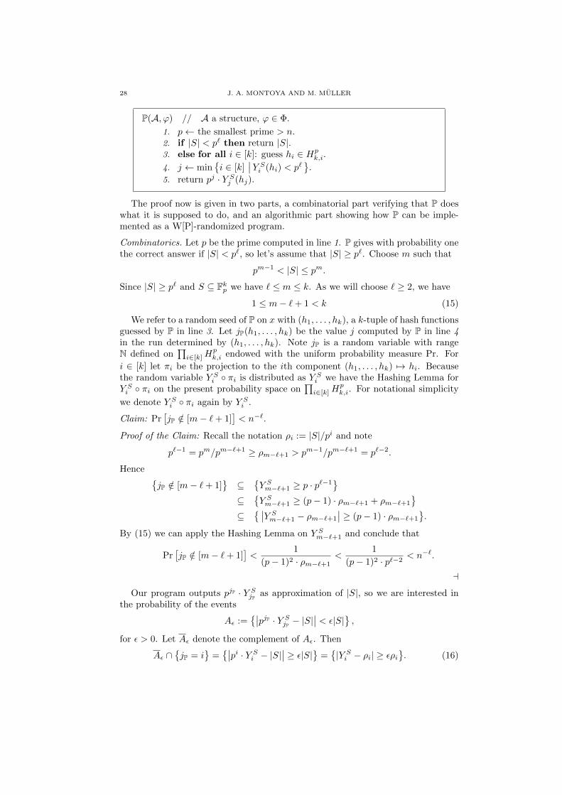
P(A, ϕ) // A a structure, ϕ ∈ Φ.

1. p← the smallest prime > n.2. if |S| < p` then return |S|.3. else for all i ∈ [k]: guess hi ∈ Hp

k,i.

4. j ← mini ∈ [k]

∣∣Y Si (hi) < p`

.

5. return pj · Y Sj (hj).

The proof now is given in two parts, a combinatorial part verifying that P doeswhat it is supposed to do, and an algorithmic part showing how P can be imple-mented as a W[P]-randomized program.

Combinatorics. Let p be the prime computed in line 1. P gives with probability onethe correct answer if |S| < p`, so let’s assume that |S| ≥ p`. Choose m such that

pm−1 < |S| ≤ pm.

Since |S| ≥ p` and S ⊆ Fkp we have ` ≤ m ≤ k. As we will choose ` ≥ 2, we have

1 ≤ m− `+ 1 < k (15)

We refer to a random seed of P on x with (h1, . . . , hk), a k-tuple of hash functionsguessed by P in line 3. Let jP(h1, . . . , hk) be the value j computed by P in line 4in the run determined by (h1, . . . , hk). Note jP is a random variable with rangeN defined on

∏i∈[k]H

pk,i endowed with the uniform probability measure Pr. For

i ∈ [k] let πi be the projection to the ith component (h1, . . . , hk) 7→ hi. Becausethe random variable Y Si πi is distributed as Y Si we have the Hashing Lemma forY Si πi on the present probability space on

∏i∈[k]H

pk,i. For notational simplicity

we denote Y Si πi again by Y Si .

Claim: Pr[jP /∈ [m− `+ 1]

]< n−`.

Proof of the Claim: Recall the notation ρi := |S|/pi and note

p`−1 = pm/pm−`+1 ≥ ρm−`+1 > pm−1/pm−`+1 = p`−2.

Hence jP /∈ [m− `+ 1]

⊆

Y Sm−`+1 ≥ p · p`−1

⊆

Y Sm−`+1 ≥ (p− 1) · ρm−`+1 + ρm−`+1

⊆

∣∣Y Sm−`+1 − ρm−`+1

∣∣ ≥ (p− 1) · ρm−`+1

.

By (15) we can apply the Hashing Lemma on Y Sm−`+1 and conclude that

Pr[jP /∈ [m− `+ 1]

]<

1

(p− 1)2 · ρm−`+1<

1

(p− 1)2 · p`−2< n−`.

a

Our program outputs pjP · Y SjP as approximation of |S|, so we are interested inthe probability of the events

Aε :=∣∣pjP · Y SjP − |S|∣∣ < ε|S|

,

for ε > 0. Let Aε denote the complement of Aε. Then

Aε ∩jP = i

=∣∣pi · Y Si − |S|∣∣ ≥ ε|S| =

|Y Si − ρi| ≥ ερi

. (16)


For i ∈ [m− `+ 1] we have ρi > pm−1/pm−`+1 = p`−2. By the Hashing Lemmawe thus get for all ε > 0 and all i ∈ [m− `+ 1]

Pr[∣∣Y Si − ρi∣∣ ≥ ερi] ≤ 1/(ε2ρi) < 1/(ε2p`−2) < 1/(ε2n`−2). (17)

Thus

Pr[Aε]

= Pr[Aε ∩

jP /∈ [m− `+ 1]

]+ Pr

[Aε ∩

jP ∈ [m− `+ 1]

]< n−` +

m−`+1∑i=1

Pr[Aε ∩

jP = i

]by the Claim

< n−` +m− `+ 1

ε2n`−2by (17) and (16).

Now, let c, c′ ≥ 1 be arbitrary. For ε := n−c the above is by (15)

≤ n−` + (k − 1)n2cn−`+2 < kn2c+2−`

and hence < n2c+3−` as we assumed k ≤ n. Choosing ` := 2c+ 3 + c′ we get

Pr[An−c

]= Pr

[P(A, ϕ) ∈ (1± n−c) · |S|

]> 1− n−c

′.

This suffices by our assumption that the size of (A, ϕ) is ≤ n2 and by Lemma 7.11(we already noted that our problem is fpt paddable).

Algorithmics. We now explain how to implement P as a W[P]-randomized program.Concerning the random complexity, note that to guess some hi ∈ Hp

k,i in line 3, Pguesses the entries of a i×k-matrix and a length i vector over Fp. Hence line 3 can

be executed by rolling∑ki=1(ik + i) = O(k3) many p-sided dice.

Concerning the time complexity we have to explain how P does the jobs wedemand it to do in fpt time.

The prime p in line 1 can be computed in polynomial time (since p < 2n+ 1 byBertrand’s Postulate). Since ` is a constant, p` ≤ nO(1).

In a first step we explain how P works using a balanced oracle for the followingauxiliary parameterized counting problem:

var-Bounded-#MC(Φ)Input: a structure B, ψ ∈ Φ and r ∈ N in unary.

Parameter: the number of variables of ψ.Problem: compute min |ψ(B)|, r.

In a second step we will show how the oracle to var-Bounded-#MC(Φ) can bereplaced by an oracle to var-MC(Φ).

Line 2 is directly solved by one balanced oracle call to var-Bounded-#MC(Φ).The remaining time needed is dominated by the computations of j in line 4 andY Si (hi) in line 5. Our program P has to solve the following problem:

Input: a structure A, ϕ ∈ Φ, h ∈ Hpk,i with i ∈ [k] (where

p is the smallest prime > |A|, ϕ has k free vari-ables, and i is determined by h).

Parameter: the number of variables of ϕ.Problem: decide if Y Si (h) < p` and if so compute Y Si (h)

(where S = ϕ(A)).


Let (A, ϕ, h) be an instance of this problem and let x = x1 · · ·xk comprise the freevariables of ϕ. Furthermore, let h be given by the i× k-matrix M and the i-vectorb over Fp.

To solve our problem with a balanced oracle for var-Bounded-#MC(Φ) itsuffices to express Y Si (h) as |ϕ∗(A∗)| for a formula ϕ∗ ∈ Φ and a structure A∗.Moreover, for the oracle to be balanced we need that the number of variables of ϕ∗

is effectively bounded in that of ϕ.We move from A to an arithmetical structure A∗: the universe of A∗ is that

of Fp; A∗ interprets all symbols as A does plus two new ternary relation symbols:

RA∗

+ :=

(a, b, c) ∈ F3p | a+ b = c in Fp

,

RA∗

× :=

(a, b, c) ∈ F3p | a · b = c in Fp

.

Further, A∗ interprets a new unary predicate A by A. Define the formula

ϕ∗ := ϕA(x) ∧∧ν∈[k]

Axν ∧ “h(x) = 0i”.

Here ϕA denotes the relativization of ϕ to A (cf. page 26). We now explain whatformula “h(x) = 0i” stands for. First, for m ∈ (A∗)k and b ∈ A∗ we introduce aformula “〈m, x〉 + b = 0” (where 〈·, ·〉 stands for the inner product of Fkp). Writemµ for the µth component of m. We use auxiliary variables uµ intended to standfor mµ · xµ and vµ to stand for the intermediate results when computing the sum〈m, x〉. Precisely, “〈m, x〉+ b = 0” is the formula∧

µ∈[k]

R×mµxµuµ ∧ v1 = u1 ∧∧

µ∈[k−1]

R+vµuµ+1vµ+1 ∧R+vkb0.

The formula is quantifier free, uses m, b and 0 as parameters and has variables xand auxiliary variables u = u1 · · ·uk and v = v1 · · · vk.

Now define “h(x) = 0i” to be the conjunction of the formulas “〈mν , x〉+ bν = 0”for ν ∈ [i], where mν denotes the νth row of M and bν the νth component of b.For each ν ∈ [i] we use a different set of auxiliary variables.

Then

|ϕ∗(A∗)| =∣∣ϕ(A) ∩ h−1(0i)

∣∣ = Y Si (h).

Moreover, ϕ∗ has i · 2k more variables than ϕ and, as Φ is robust, ϕ∗ ∈ Φ.

We are left to show that var-Bounded-#MC(Φ) is fixed-parameter tractableusing a balanced oracle for the decision problem var-MC(Φ).

But var-MC(Φ) is ‘self-reducible’. It follows by general means that there isan algorithm A (and we shall define such an algorithm below) using a balancedoracle for var-MC(Φ) that solves the associated listing problem with fpt delay [43]:A on an instance (B, ψ) of var-MC(Φ) outputs without repetitions all tuples inψ(B) such that the delay of A is fpt bounded; here delay means the maximumnumber of steps until the first output, between any two outputs and from the lastoutput to the halting configuration (see [46]). Granted such an algorithm A, weproceed straightforwardly: let (B, ψ, r) be an instance of var-Bounded-#MC(Φ);on (B, ψ, r) simulate A on (B, ψ); increase a counter (initialized by 0) for eachoutput of A; stop the simulation in case the counter becomes r; return the counter.The time needed here is roughly r times the delay of A and thus fpt bounded.


We describe the algorithm A: on (B, ψ) it runs A′ on (B, ψ, λ) for the emptytuple λ. Algorithm A′ takes inputs (B, ψ, b) for structures B, ψ ∈ Φ, and b a tupleover B. For b ∈ B let ψb := ψ b

x for x the first free variable in ψ (and undefined if

ψ is a sentence). A′ on (B, ψ, b) is the following recursive procedure:

A′(B, ψ, b) // B a structure, ψ ∈ Φ and b a tuple over B.

1. if ψ(B) = ∅ then stop.2. else if ψ has no free variables then return b3. else for all b ∈ B do4. return A′(B, ψb, bb)

(Note that for a sentence ψ we have ψ(B) ∈ ∅, λ.) Algorithm A′ uses an oraclefor var-MC(Φ) to check the if-condition in line 1. It is routine to verify that thisdefines a listing algorithm as desired.

8. Uniqueness promises

8.1. A logical form of the Valiant-Vazirani Lemma. In classical complexitytheory the famous Valiant-Vazirani Lemma states that “the problems of distin-guishing between instances of Sat having zero or one solution, or finding solutionsto instances of Sat having unique solutions, are as hard as Sat itself” ([66, Ab-stract]). Here hardness refers to randomized reductions with one-sided error. Thisresult can be shaped as a probabilistic statement about Boolean logic:

Theorem 8.1 (Valiant, Vazirani 1985). There is a polynomial time algorithm com-puting for any Boolean formula α(X) a Boolean formula β(XY ) such that, if α issatisfiable, then

Prb∈0,1|Y |

[b |= ∃=1X

(α(X) ∧ β(XY )

)]> 1/10 · |X|−1.

It is easy to see that we can also allow the formula α to come from Boolean logicextended by various quantifiers. In this section we intend to show such results forlogics beyond Boolean logic. We show that given a structure A and a formula ϕ ofleast fixed-point logic LFP we can do the following in polynomial time: first, we en-large A by increasing its universe and declare some additional (mainly arithmetical)relations on it; second, we compute a formula ψ of roughly the same logical com-plexity as ϕ such that if you randomly assign values to some distinguished variablesof ψ, then in the new structure with ‘good’ probability ψ singles out exactly oneof the solutions of ϕ in A provided there are any; furthermore we have one-sidederror in the sense that ψ has no solution in case ϕ has none. To make this precisewe employ the following mode of speech:

Definition 8.2. A τ∗-enlargement of a τ -structure A is a (τ ∪ τ∗)-structure A∗which is an expansion of an extension of A such that there is some unary relationsymbol A ∈ τ∗ \ τ with AA

∗= A.

Then the main result of this section reads:

Theorem 8.3. Let τ be a vocabulary. There is a relational vocabulary τ∗ and apolynomial time algorithm which, given a τ -structure A and ϕ = ϕ(x) ∈ LFP[τ ],


computes a τ∗-enlargement A∗ of A and a quantifier free formula ρ = ρ(xyz) ∈FO[τ∗] with parameters in A∗ such that, if ϕ(A) 6= ∅, then

Prb∈(A∗)|y|

[A∗ |= ∃=1xz

(ϕA(x) ∧ ρ(xyz)

) by

]> |A∗|−2.

Furthermore, the length of ρ is polynomially bounded in |x|.

Here ϕA is the relativization of ϕ to A (see page 26).

This allows us to move in polynomial time to a ‘probably unique’ formula withoutessentially increasing the logical complexity of the input formula. The ‘probablyunique’ formula can be seen as an ordinary LFP-formula where certain designatedindividual variables are interpreted randomly in A∗. This is the view taken inK.Eickmeyer and M.Grohe’s randomized logics [31].

The logic LFP does not play an essential role here and could be replaced bycertain abstract logics in the sense of [30]. We state the result for LFP for simplicityand because it suffices for the applications we have in mind.

8.2. Corollaries on uniqueness promises. Theorem 8.1 has proven useful inmany respects. For example it is a main step in Toda’s [64] original proof thatPH ⊆ BP ⊕ P ⊆ P#P. Because of these applications some work has been done onimproving the involved parameters, especially the number of random bits [60, 15].

Another application of Theorem 8.1 concerns the problem

USatInput: a CNF α.

Problem: does α have exactly one satisfying assignment?

This problem has received considerable attention [66, 6, 14, 13, 42, 12]. It is knownto be coNP-hard and contained in the class DP4. Moreover it has, in some sense,the same exponential time complexity as Sat [42, 12].

Theorem 8.1 gives a randomized reduction of NP problems to Sat with unique-ness promise, i.e. such that output formulas probably either have exactly one so-lution or no solution at all. This implies that USat is NP-hard under randomizedpolynomial time reductions with one-sided error. The reductions have an inversepolynomial success probability, and, in fact, USat is complete for DP under suchreductions [66, Corollary 5] (see [14] for a discussion).

Corollary 8.4. If NP 6⊆ RP, then USat /∈ P.

R.G.Downey, M.R.Fellows and K.W.Regan [29] ask for analogues of these resultsin the parameterized setting. They proved the following. Recall the definition ofthe problem p-WSat(Ωt,d) from page 4.

Theorem 8.5 (Downey, Fellows, Regan 1998). Let t ≥ 1. There is a d ∈ N suchthat for all (Q, κ) ∈ W[t] there is a randomized reduction with one-sided fpt errorfrom (Q, κ) to p-WSat(Ωt,d) with uniqueness promise.

4DP is sometimes written DP and comprises the differences of NP problems; [27, Exercise 16.04]introduces a parameterized ‘stratification’ of this class.


Informally, such a reduction probably produces instances having either exactlyone or no solution. “Probably” refers to an inverse fpt success probability, i.e.1/(f(k) · nc) for some computable f : N → N and c ∈ N (cf. Definitions 8.10 hereand 6.1 in [29]). The reductions constructed in [29] use k · n · log n random bits.They actually, achieve a better error bound of order 1/(f(k) · log n).

With an eye on the goal of finding some parameterized analogue of Toda’s the-orem Downey et al. [29] asked how to derandomize their reduction to – in thepresent terminology – W[P]-randomized reductions. The following result answersthis question affirmatively for all classes of the A-matrix and more:

Theorem 8.6. Let (Q, κ) be a parameterized problem. Then

(1) if (Q, κ) ∈ A[`, t], then there is a W[1]-randomized reduction with one-sidedfpt error to p-MC(Σ`,t−1,1) with uniqueness promise.

(2) if (Q, κ) ∈ W[SAT], then there is a W[1]-randomized reduction with one-sided fpt error to var-MC(Σ1) with uniqueness promise.

(3) if (Q, κ) ∈W[P], then there is a W[1]-randomized reduction with one-sidedfpt error to var-MC(Σ1LFP[1]) with uniqueness promise.

The main message of this result is, roughly, that hard problems remain hard (ina randomized sense) even with a uniqueness promise. E.g. an fpt algorithm solving

p-CliqueInput: a graph G and k ∈ N.

Parameter: k.Problem: does G contain a k-clique?

with uniqueness promise would be an algorithm which behaves like an fpt algorithmfor p-Clique provided it is fed with an input (G, k) such that G either has exactlyone or no k-clique; on other instances the algorithm may do whatever it wants(cf. Definition 8.11).

A second message of Theorem 8.6 is, roughly, that ‘uniqueness-versions’ of hardproblems are hard too. Specifically, [29] and [28] asked for the complexity of

p-UCliqueInput: a graph G and k ∈ N.

Parameter: k.Problem: does G contain exactly one k-clique?

We get the following parameterized analogue of Corollary 8.4:

Corollary 8.7. If W[1] 6⊆ RFPT, then p-Clique with uniqueness promise is notfixed-parameter tractable, and in particular, p-UClique /∈ FPT.

This is not a special property of the clique problem and we shall prove somethingmore general (Theorems 8.17 and 8.18).

Remark 8.8. As for an an upper bound on the complexity of p-UClique firstobserve that W[1] contains the problem p-Two-Cliques that asks, given a graphG and a parameter k, whether G contains at least two k-cliques. Hence this problemis fpt reducible to p-Clique. But p-UClique is the intersection of p-Clique and


the complement of p-Two-Cliques. So two non-adaptive, balanced oracle queriesto p-Clique suffice to decide p-UClique.

Remark 8.9. In [19] Y.Chen and J.Flum apply Theorem 8.3 to show that certaincounting problems are not #W[1]-hard unless W[1] ⊆ RFPT.

8.3. Proof of Theorem 8.3. Let ϕ(x) ∈ LFP[τ ] be a formula and A be a τ -structure. Let k := |x|. If |A| = 1, we take ρ := y = y and asA∗ any τ∗-enlargementof A with A∗ = A. The same works in case k = 0, since then ϕ(A) either containsnothing or exactly the empty tuple. Hence we can assume k ≥ 1, |A| ≥ 2 andA = 0, . . . , |A|−1. We can further assume that k ≥ 3 and that 0 (the all 0 k-tuple)does not satisfy ϕ in A. To see this, note that ϕ(xx1x2) := ϕ(x) ∧ x1 = 1 ∧ x2 = 1(where 1 is a parameter) satisfies this assumption and |ϕ(A)| = |ϕ(A)|; if A∗ andρ(xx1x2yz) satisfy our claim for ϕ, then A∗ and ρ(xyz′) := x1 = 1 ∧ x2 = 1 ∧ ρwith z′ := zx1x2 satisfy our claim for ϕ(x).

Construction of A∗. Let p be the smallest prime bigger than |A| and k + 2. ByBertrand’s Postulate we can compute p in polynomial time. The structure A∗ hasuniverse

A∗ := 0, . . . , k · p− 1.We set τ∗ := R+, R×, Rmod, A,≤ for ternaryR+, R×, Rmod, binary≤ and unary A.We let A∗ be a τ∗-enlargement of A with

AA∗

:= A,

RA∗

+ := (a, b, c) ∈ (A∗)3 | a+ b = cmod p,RA

∗

× := (a, b, c) ∈ (A∗)3 | a · b = cmod p,RA

∗

mod := (a, b, c) ∈ (A∗)3 | a < c and a = bmod c,≤A

∗:= the natural order on A∗.

In A∗ the set 0, . . . , p−1 carries the structure of Fp, the field with p elements.The set of solutions ϕ(A) ⊆ Ak ⊆ Fkp lives in the k-dimensional vectorspace over Fp.

The hyperplanes Ha. For a vector a ∈ Fkp \ 0 let 〈a〉⊥ denote the hyperplane of

vectors orthogonal to a. If we translate 〈a〉⊥ by a we get Ha, that is

Ha := 〈a〉⊥ + a =b+ a | b ∈ 〈a〉⊥

.

This is a hyperplane in Fkp and hence

|Ha| = pk−1. (18)

Let a, b ∈ Fkp \ 0 be distinct. If a and b are linearly independent, the hyperplanesHa and Hb are not parallel and so the affine subspace Ha∩Hb has dimension k−2.If a and b are linearly dependent, then Ha ∩Hb = ∅ (it is herefore that we use thetranslation Ha instead of 〈a〉⊥). In particular

|Ha ∩Hb| ≤ pk−2. (19)

To prove the classical Valiant-Vazirani Lemma one typically splits the spacecontaining the solutions (there a cartesian power of 0, 1) randomly in half for arandom number of times, and analyzes the probability that exactly one solutionremains. We argue similarly. Our solutions are contained in Fkp. An idea now isto cut down this space to a 1/p-fraction using random hyperplanes and to do so


subsequently for a random number of times. We do not select random hyperplanesbut a random number of random vectors from Fkp and look at the event that allthese are contained in a hyperplane Ha associated with a solution a ∈ ϕ(A). Wethen bound from below the probability that the above event holds for exactly onesolution. It is here where we need that 0 /∈ ϕ(A). Details follow.

Construction of ρ. Intuitively, the following formula wants x from A such that thefirst u+ 2 of y1, . . . , yk+2 ∈ Fkp are in Hx:

ρ′ :=∧j∈[k]

Axj ∧∧

i∈[k+2]

“y′i = yi mod p” ∧Rmodu′u(k + 1)

∧∧

i∈[k+2]

(maxi− 2, 0 ≤ u′ → “y′i ∈ Hx”

).

This formula uses 0, . . . , k+1 and p as parameters from A∗. Further “y′i = yi mod p”abbreviates the formula

∧j∈[k]Rmody

′ijyijp, where we write e.g. y1 = y11 · · · y1k. We

now explain for what formula “y ∈ Hx” stands for.Observe that, loosely written, y ∈ Hx if and only if

∑j(yj − xj) · xj = 0. We

introduce auxiliary variables for all intermediate results obtained when computingthis sum, namely we intend uj = yj − xj , the vj ’s to denote the products summedand the wj ’s to denote the partial sums obtained when adding up the vj ’s. Precisely,we let “y ∈ Hx” stand for the formula:∧

j∈[k]

R+ujxjyj ∧∧j∈[k]

R×ujxjvj ∧∧

j∈[k−1]

R+wjvjwj+1 ∧ w1 = v1 ∧ wk = 0.

So “y ∈ Hx” is a formula in the variables xyuvw and with parameter 0. In ρ′ weuse for each i ∈ [k + 2] distinct auxiliary variables uiviwi in “y′i ∈ Hx”, that is,“y′i ∈ Hx” has free variables xy′iuiviwi.

We aim at a formula ρ such that with good probability for a random assignment

to the yi and u we have exactly one solution of (ϕA ∧ ρ). So far this cannot worksince we can assign whatever we want to the auxiliary variables uiviwi for i largerthan the value of u′ plus 2. We set

ρ := ρ′ ∧∧

i∈[k+2]

(¬maxi− 2, 0 ≤ u′ → “uiviwi = 0”).

In the notation of our claim we let y comprise all the yi’s and u and we let zcomprise all primed variables as well as all the auxiliary variables uiviwi.

This completes the construction of A∗ and ρ. It is clear that A∗ and ρ can becomputed in polynomial time given A and ϕ.

Probability analysis. Assume ϕ(A) 6= ∅. Let b ∈ A∗ and b1, . . . , bk+2 ∈ (A∗)k bearbitrary and abbreviate

ψ := (ϕA ∧ ρ)b

u

b1 · · · bk+2

y1 · · · yk+2.

The assignment of a to x can be extended to an assignment satisfying ψ in A∗ ifand only if a ∈ ϕ(A) and (bi mod p) ∈ Ha for all i ∈ [(bmod (k+1))+2]. Moreover,in this case there is exactly one such extension. In particular

|ψ(A∗)| =∣∣a ∈ ϕ(A) | bi mod p ∈ Ha for all i ∈ [(bmod (k + 1)) + 2]

∣∣ . (20)


We define a function f by

f(bb1 · · · bk+2

):=

∣∣∣∣(ϕA ∧ ρ)b

u

b1 · · · bk+2

y1 · · · yk+2(A∗)

∣∣∣∣ .Think of the set of the bb1 · · · bk+2’s as carrying a probability space with the uniformprobability measure. Declare two points bb1 · · · bk+2 and b′b′1 · · · b′k+2 of this space to

be equivalent if b ≡ b′mod (k+1) and componentwise bi ≡ b′i mod p for all i ∈ [k+2].Then the event f = 1 is a union of such equivalence classes. All equivalenceclasses have the same size since both p and k divide |A∗| (therefore we chose A∗ aswe did). Thus, the probability that f is 1 on a random argument bb1 · · · bk+2 is thesame as the probability that f is 1 on an argument chosen uniformly at randomfrom those bb1 · · · bk+2 with b < k + 1 and bi ∈ Fkp for all i ∈ [k + 2].

Let B,B1, . . . , Bk+2 be independent random variables such that B is uniformlydistributed in 0, . . . , k and each Bi is uniformly distributed in Fkp. Then the

theorem claims Pr [f(BB1 · · ·Bk+2) = 1] ≥ 1/|A∗|2.To prove this, call m good if

pm ≤ |ϕ(A)| ≤ pm+1.

Since 1 ≤ |ϕ(A)| ≤ |A|k ≤ pk we have 0 ≤ m ≤ k for any good m. HencePr[B is good] is at least 1/(k + 1). If we could find some t such that

Pr[f(mB1 · · ·Bk+2) = 1] > t

for all good m, then we would know the following: for at least a 1/(k + 1) frac-tion of b’s we find at least a t fraction of b1 · · · bk+2’s such that f is 1; hencePr[f(BB1 · · ·Bk+2) = 1] > t/(k + 1).

Claim 1: If m is good, then Pr[f(mB1 · · ·Bk+2) = 1

]> 1/(2p2).

This implies the theorem: 1/((k + 1)2p2) ≥ 1/(k2p2) = 1/|A∗|2 (as k ≥ 3).

Proof of Claim 1: Let m be good. By (20)

f(mB1 · · ·Bk+2) = |a ∈ ϕ(A) | B1, . . . , Bm+2 ∈ Ha|.Hence f(mb1 · · · bk+2) = 1 if and only if there is a solution a ∈ ϕ(A) such that Ha

contains all b1, . . . , bm+2 but there is no other solution with this property. Definefor a ∈ ϕ(A) the event

Am(a) := B1, . . . , Bm+2 ∈ Ha ∩⋂

a′∈ϕ(A)\a

⋃i∈[m+2]

Bi /∈ Ha′. (21)

Then Am(a) ∩Am(a′) = ∅ for distinct a, a′ ∈ ϕ(A) and

f(mB1 · · ·Bk+2) = 1 =⋃

a∈ϕ(A)

Am(a). (22)

Using the following Claim 2 we get what we want:

Pr[f(mB1 · · ·Bk+2) = 1

]=

∑a∈ϕ(A)

Pr[Am(a)] >∑

a∈ϕ(A)

p− 1

pm+3≥ pm(p− 1)

pm+3≥ 1

2p2.

Here, the equality is due to (22), the first inequality to Claim 2 below and thesecond inequality to m being good. a

We are thus left to verify:

Claim 2: If m is good, then Pr[Am(a)] > (p− 1)/pm+3 for all a ∈ ϕ(A).


Proof of Claim 2: Let m be good, a ∈ ϕ(A) and write B := (B1, . . . , Bm+2).By (18)

Pr[B ∈ Hm+2

a

]=

∏i∈[m+2]

Pr [Bi ∈ Ha] = 1/pm+2. (23)

For any a′ ∈ ϕ(A) \ a we have by (19) (note a, a′ 6= 0)

Pr[B ∈ (Ha ∩Ha′)

m+2]

=∏

i∈[m+2]

Pr [Bi ∈ Ha ∩Ha′ ] ≤ 1/p2(m+2). (24)

By (23) and (24)

Pr[B ∈ Hm+2

a′ | B ∈ Hm+2a

]≤ 1/pm+2. (25)

Letting a′ range over ϕ(A) \ a we conclude

Pr [Am(a)] = Pr[B ∈ Hm+2

a

]· Pr

[⋂a′

⋃i∈[m+2]

Bi /∈ Ha′∣∣∣ B ∈ Hm+2

a

]≥ Pr

[B ∈ Hm+2

a

]·(

1−∑a′

Pr[B ∈ Hm+2

a′

∣∣∣ B ∈ Hm+2a

])≥ 1

pm+2·(

1− |ϕ(A)| − 1

pm+2

)>

1

pm+2·(

1− pm+1

pm+2

)=p− 1

pm+3.

The equality follows from definition (21), the first inequality from the union bound,the second inequality from (23) and (25), and the third from m being good.

8.4. Proofs of the corollaries. To prove the results announced in Section 8.2,we need to make two things precise (Definitions 8.10 and 8.11 below), namely, wehave to define the randomized reductions to promise problems as mentioned inTheorems 8.5 and 8.6 and we have to define what it means to decide a problemwith uniqueness promise in fpt time (as mentioned in Corollary 8.7).

Usually, if (F, κ) is the naturally associated counting version of a decision prob-lem (Q, κ), then Q = F > 0(= x ∈ Σ∗ | F (x) > 0). But, of course F > 0does not determine F , so the modes of speech we are going to introduce are appli-cable only within a context determining F . This obligation vanishes when talkingabout decision problems having – by agreement – a certain naturally associatedcounting problem. This is the case for model-checking problems.

Definition 8.10. Let (Q, κ) be a parameterized decision problem and let (F, κ′)be a parameterized counting problem. A (W[1]-, W[P]-)randomized reduction withone-sided fpt error from (Q, κ) to (F > 0, κ′) with uniqueness promise is a (W[1]-,W[P]-)randomized program P such that there are computable f, g : N → N and ac ∈ N such that for all x ∈ Σ∗:

(1) if x ∈ Q, then Pr[F (P(x)) = 1] ≥ 1/(f(κ(x)) · |x|c);(2) if x /∈ Q, then Pr[F (P(x)) = 0] = 1;(3) Pr[κ′(P(x)) ≤ g(κ(x))] = 1.

Definition 8.11. Given a parameterized counting problem (F, κ), we say that(F > 0, κ) with uniqueness promise is fixed-parameter tractable if there are analgorithm A and a computable f : N → N such that for all x ∈ Σ∗ with F (x) ∈0, 1:


(1) A runs in time f(κ(x)) · |x|O(1);(2) A accepts x⇐⇒ x ∈ F > 0.

Remark 8.12. One could equivalently demand A to be fpt time bounded: equipan algorithm as in Definition 8.11 with a clock; if time runs out the input x doesnot satisfy F (x) ∈ 0, 1 and we can answer arbitrarily.

Proposition 8.13. Let (Q, κ) be a parameterized decision problem outside RFPTand let (F, κ′) be a parameterized counting problem. Assume there is a W[P]-randomized reduction with one-sided fpt error from (Q, κ) to (F > 0, κ′) withuniqueness promise. Then (F > 0, κ′) with uniqueness promise is not fixed-parameter tractable.

Proof. First apply the reduction from (Q, κ) to (F > 0, κ′) and then an fpt timebounded (Remark 8.12) algorithm witnessing that (F > 0, κ′) with uniquenesspromise is fixed-parameter tractable. This decides (Q, κ) in fpt time with one-sidederror at most 1−1/(h(κ(x))·|x|c) for some computable h : N→ N and some constantc ∈ N. In particular, Q is decidable. But the error 1− 1/(h(κ(x)) · |x|c) is at most1−|x|−(c+1) on those instances x of length at least h(κ(x)). On other inputs we canrun some decision procedure for Q; this needs time effectively bounded in κ(x). Weconclude that (Q, κ) can be decided by a W[P]-randomized program with one-sidederror 1− |x|−(c+1). Thus (Q, κ) ∈ RFPT by Theorem 4.1 (and Remark 4.2).

To prove Theorem 8.6 we use the following straightforward lemma:

Lemma 8.14. Let (F, κ′′) be a parameterized counting problem and (Q, κ), (Q′, κ′)be parameterized decision problems such that (Q, κ) is fpt reducible to (Q′, κ′). Ifthere is a W[1]-randomized reduction with one-sided fpt error from (Q′, κ′) to (F >0, κ′′) with uniqueness promise, then also from (Q, κ) to (F > 0, κ′′).

Proof of Theorem 8.6: To prove (1) or (2) or (3) we can, by Lemma 8.14, assumethat (Q, κ) = (MC(Φ), κ) where Φ is some suitable class of LFP formulas andand κ is either the parameterization by the length of the input formula or thenumber of its variables. A program computing the desired reduction works asfollows: given an instance (A, ϕ(x)) of MC(Φ) first compute deterministically A∗

and (ϕA(x) ∧ ρ(xyz)) from Theorem 8.3 in polynomial time. Then roll |y| many

|A∗|-sided dice to get b ∈ (A∗)|y| and output(A∗, (ϕA ∧ ρ) by

).

Note (ϕA ∧ ρ) ∈ Φ, whenever ϕ ∈ Φ modulo an easy polynomial time modifi-cation. As the length of ρ and hence also |y| is polynomially bounded in |x|, ourprogram is W[1]-randomized and satisfies Definition 8.10 (3). Definition 8.10 (2) is

satisfied too, because in case ϕ(A) = ∅ we have (ϕA∧ρ) by (A∗) = ∅ for all b. Other-

wise |(ϕA ∧ ρ) by (A∗)| = 1 with probability at least 1/|A∗|2. As |A∗| is polynomially

bounded in the input size, Definition 8.10 (1) is satisfied.

Remark 8.15. The argument given shows more than stated. It proves analo-gous statements also for the classes of the W∗-hierarchy, the classes of the Wfunc-hierarchy and the classes AW[∗], AW[SAT] and AW[P]. See [37, Chapter 8] for suit-able model-checking characterizations of these classes except AW[P]. For AW[P]see [21, Theorem 33(2)].

The following is easy to see.


Lemma 8.16. Let (F, κ) and (F ′, κ′) be parameterized counting problems such that(F, κ) is fpt reducible to (F ′, κ′). If (F ′ > 0, κ′) with uniqueness promise is fixed-parameter tractable, then (F > 0, κ) with uniqueness promise is fixed-parametertractable.

Theorem 8.17. Let `, t ≥ 1 and let (F, κ) be a #A[`, t]-hard parameterized count-ing problem. Then (F > 0, κ) with uniqueness promise is not fixed-parametertractable unless A[`, t] ⊆ RFPT.

Proof. Let `, t ≥ 1 and (F, κ) be as stated. If (F > 0, κ) with uniqueness promiseis fixed-parameter tractable, then so is p-MC(Π`−1,t−1,1) by Lemma 8.16. ThenA[`, t] ⊆ RFPT by Proposition 8.13 and Theorem 8.6.

Concerning ‘uniqueness variants’ of decision problems this yields:

Theorem 8.18. Let `, t ≥ 1 and let (F, κ) be a #A[`, t]-hard parameterized count-ing problem. Then (F = 1, κ) /∈ FPT unless A[`, t] ⊆ RFPT.

Proof. By Theorem 8.17 it suffices to note that an fpt algorithm for (F = 1, κ)witnesses that (F > 0, κ) with uniqueness promise is fixed-parameter tractable.

Since p-#Clique is #W[1]-complete, the two claims of Corollary 8.7 follow fromthe previous two theorems.

9. Questions

We saw some first steps of parameterized random complexity theory and manyquestion are open. Answers to the following ones may advance more generally ourunderstanding of structural parameterized complexity theory.

Section 3 (Parameterized randomization: basic observations and techniques). Thesection defined two modes of parameterized randomization corresponding to takingW[1] or W[P] as parameterized analogue of NP. Concerning the characterizationof randomized parameterized tractability by randomized kernelizations it would beinteresting to know whether randomized kernelizations can beat deterministic oneswith respect to kernel size.

Section 4 (Deterministic probability amplification). The section established strongprobability amplification for W[P]-randomization. Can you amplify W[1]-rando-mized two-sided error from 1

2 −1|x| to 1

4 or from 14 to 1

|x|? We are not aware of

amplifications methods that are useful in this respect, so the question may be astarting point to find new such methods.

Section 5 (Parameterized derandomization). The section characterized (“black-box”)derandomization of BPFPT in terms of classical derandomization. What doesBPFPT[1] = FPT mean in such terms? The question points to the problemthat W[1] does not have a nice characterization by Turing machines (see however[11, 29]). Or can you prove BPFPT[1] = FPT unconditionally?


Section 6 (Upper bounds). The section gave analogues of the Sipser-Gacs Theo-rem for both W[P]- and W[1]-randomization. Is there an analogue of Adleman’sTheorem, that is, does parameterized randomized tractability imply some form ofnon-uniform parameterized tractability? Adleman’s line of argument breaks at thepoint where the analogy of the parameterized class XP and the classical class EXPis flawed: there are more than nf(k) instances of size n with parameter k. A struc-tural question seemingly of relevance here is: what kind a problem (Q, κ) has anfpt reduction r to itself such that the range of r is polynomial time decidable andcontains at most nf(k) instances of size n with parameter k?

Does W[1] = FPT imply BPFPT[1] = FPT? The structural problem behindthis question is the lack of a collapse theorem for the A-hierarchy.

Section 7 (Probably almost correct counting). The section gave analogues of a The-orem of Stockmeyer. Under what conditions do we have these theorems ‘problem-wise’? That is: when approximating a counting problem coming from a decisionproblem (Q, κ), say (Q, κ) ∈W[1], are we really in need of an oracle for the full classW[1] or could we do with (Q, κ)? Trivially, the answer is yes for W[1]-hard (Q, κ).But the question is interesting for problems in FPT with a #W[1]-hard countingversion. An answer would constitute a step towards a theoretical understandingof what it is that makes certain hard counting problems have fast randomized ap-proximations.

Another open question is whether one can derandomize the result of V.Arvindand V.Raman (see page 25) to W[P]-fptrases.

Section 8 (Uniqueness promises). We proved a general ‘logical’ version of the Valiant-Vazirani Lemma applicable to all classes of the A-matrix. An important questionis whether we can achieve a better success probability, say, of at least 1/k? Thisquestion comes from the struggle for a parameterized analogue of Toda’s Theorem,repeatedly asked for in [29, 28, 35, 37]. The first author obtained some conditional

results [50]. Such an analogue would state that FPT#W[1] contains the A-hierarchy

or at least the W-hierarchy, or that FPT#W[P] contains the AWP-hierarchy (cf. Def-inition 6.1) or at least the A-hierarchy.

References

[1] M.Ajtai, J.Komlos, and E.Szemeredi, Deterministic simulation in LOGSPACE, Proceedings

of the 9th annual ACM Symposium on Theory of Computing (STOC’87), pp.132-140, 1987.[2] M.Alekhnovich and A.A.Razborov, Resolution is not automatizable unless W[P] is tractable,

Proceedings of the 41th IEEE Symposium on Foundations of Computer Science (FOCS’01),

pp- 210-219, 2001.[3] N.Alon, R.Yuster, and U.Zwick, Color-coding, Journal of the ACM 42, pp.844-856,1995.

[4] S.Arora and B.Barak, Computational Complexity: A Modern Perspective, Cam-

bridge University Press, 2009.[5] V.Arvind and V.Raman, Approximation algorithms for some parameterized counting prob-

lems. In I.Bose and P.Morin, ed., Proceedings of the 13th International Symposium onAlgorithms and Computation, LNCS 2518, pp.453-464. Springer, 2002.

[6] A.Blass and Y.Gurevich, On the unique satisfiability problem, Information and Computation

55, pp.80-88, 1982.[7] R.P.Brent, D.J.Kuck and K.Maruyama, The parallel evaluation of arithmetic expressions

without division, IEEE Transactions on Computers C-22, pp.532-534, 1973.

[8] R.P.Brent, The parallel evaluation of general arithmetic expressions, Journal of the ACM21(2), pp.201-206, 1974.


[9] P.Bremaud, Markov Chains, Gibbs Fields, Monte Carlo Simulation and Qeues,Springer Texts in Applied Mathematics 31, 1999.

[10] L.Cai, Random separation: a new method for solving fixed-cardinality optimization prob-

lems, Proceedings of the 2nd International Workshop on Parameterized and Exact Compu-tation (IWPEC’06), LNCS 4169, pp.239-250, 2006.

[11] L.Cai, J.Chen, R.G.Downey and M.R.Fellows, On the structure of parameterized problems

in NP, Information and Computation 123, pp.38-49, 1995.[12] C.Calabro, R.Impagliazzo, V.Kabanets and R.Paturi, The complexity of unique k-SAT: an

isolation lemma for k-CNFs, Proceedings of the 18th IEEE Conference on ComputationalComplexity (CCC’03),pp.135-141, 2003.

[13] R.Chang and J.Kadin, On computing boolean connectives of characteristic functions, Theory

of Computing Systems 28 (3), pp.173-198 Springer, 1995.[14] R.Chang, J.Kadin, and P.Rohatgi, On unique satisfiability and the threshold behavior of

randomized reductions, Journal of Computer and System Sciences, 50(3), pp.359–373, 1995.

[15] S.Chari, P.Rohatgi and A.Srinivasan, Randomness-optimal unique element isolation, withapplications to perfect matching and related problems, Proceedings of the twenty-fifth ACM

Symposium on Theory of Computing (STOC’93), pp.458-467, 1993.

[16] J.Chen, S.Lu, S.-H.Sze and F.Zhang, Improved algorithms for path, matching and pack-ing problems, Proceedings of the 18th ACM-SIAM Symposium on Discrete Algorithms

(SODA’07), pp.298-307, 2007.

[17] J.Chen, Randomized disposal of unknowns and implicitly enforced bounds on parameters,Proceedings of the 3rd International Workshop on Parameterized and Exact Computation

(IWPEC’08) in Victoria, LNCS 5018, pp.1-8, 2008.

[18] Y.Chen, Model-Checking Problems, Machines and Parameterized Complexity,Dissertation, Albert-Ludwigs-Universitat Freiburg i.Br., 2004.

[19] Y.Chen and J.Flum, The parameterized complexity of maximality and minimality problems,Annals of Pure and Applied Logic 151(1), pp.22-61, 2008.

[20] Y. Chen and J. Flum, Subexponential time and fixed-parameter tractability: exploiting the

miniaturization mapping, In: Proceedings of the 21st International Workshop on ComputerScience Logic (CSL’07), LNCS 4646, pp.389-404, 2007.

[21] Y.Chen, J.Flum and M.Grohe, Bounded nondeterminism and alternation in parameterized

complexity theory, In Proceedings of the 18th IEEE Conference on Computational Com-plexity (CCC’03), pp.13-29, 2003.

[22] Y.Chen, J.Flum and M.Grohe, Machine-based methods in parameterized complexity theory,

Theoretical Computer Science 339, pp.167-199, 2005.[23] Y.Chen, J.Flum and M.Muller, Lower bounds for kernelizations and other preprocessing

procedures, Theory of Computing Systems, 48(4):803-839, 2011.

[24] Y.Chen and M.Grohe, An isomorphism between subexponential and parameterized complex-ity theory, SIAM Journal on Computing, 37(4), pp.1228-1258, 2007.

[25] S.A.Cook and R.A.Reckhoff, Time bounded random access machines, Journal of Computerand System Sciences 7, pp.354-375, 1973.

[26] R.G.Downey, V.Estivill-Castro, M.R.Fellows, E.Prietoc and F.A.Rosamond, Cutting up is

hard to do: the parameterised complexity of k-cut and related problems, in J.Harland (ed.),Proceeding of the Australasian Theory Symposium (CATS’03), Electronic Notes in Theo-

retical Computer Science 78, pp.209-222, 2003.

[27] R.G.Downey and M.R.Fellows, Parameterized Complexity, Springer, 1999.[28] R.G.Downey and M.R.Fellows, Parameterized complexity after almost ten years: review

and open questions, Proceedings of Combinatorics, Computation and Logic, DMTCS’99and CATS’99, Australian Computer Science Communications 21, Springer, pp.1-33, 1999.

[29] R.G.Downey, M.R.Fellows and K.W.Regan, Parameterized Circuit Complexity and the W

Hierarchy, Theoretical Computer Science 191(1-2), pp.97-115, 1998.

[30] H.D.Ebbinghaus, Extended Logics: The general framework, in: Model-Theoretical Logics,ed. J.Barwise, S.Feferman, Springer-Verlag, pp.25-76, 1985.

[31] K.Eickmeyer and M.Grohe, Randomisation and derandomisation in descriptive complexitytheory, Proceedings of the 24th International Workshop Computer Science Logic (CSL’10),

2010.


[32] K.Eickmeyer, M.Grohe and M.Grubner, Approximisation of W[P]-complete minimisa-tion problems is hard, Proceedings 23rd IEEE Conference on Computational Complexity

(CCC’08), pp.8-18, 2008.

[33] M.R.Fellows and N.Koblitz, Fixed-parameter complexity and cryptography, Proceedings ofthe 10th International Symposium on Applied Algebra, Algebraic Algorithms and Error-

Correcting Codes (AAECC’93), LNCS 673, pp.121-131, Springer, 1993.

[34] J.Flum and M.Grohe, Fixed-parameter tractability, definability, and model checking, SIAMJournal on Computing 31, pp.113-145, 2001.

[35] J.Flum and M.Grohe, The parameterized complexity of counting problems, SIAM Journalon Computing 33(4), pp.892-922, 2004.

[36] J.Flum and M.Grohe, Model-checking problems as a basis for parameterized intractability,

Logical Methods in Computer Science 1(1), 2005. Conference version in Proceedings of the19th IEEE Symposium on Logic in Computer Science (LICS’04), pp.388-397, 2004.

[37] J.Flum and M.Grohe, Parameterized Complexity Theory, Springer, 2006.

[38] J.Flum, M.Grohe and M.Weyer, Bounded fixed-parameter tractability and log2 n nondeter-ministic bits, Journal of Computer and System Sciences 72, pp.34-71, 2006.

[39] O.Goldreich, Introduction to complexity theory - Lecture Notes, 2001; available at

http://www.wisdom.weizmann.ac.il/~oded/homepage.html.[40] O.Goldreich, Randomized methods in computation - Lecture Notes, 2001; available at

http://www.wisdom.weizmann.ac.il/~oded/homepage.html.

[41] O.Goldreich, Computational Complexity: A Conceptual Perspective, CambridgeUniversity Press, 2008.

[42] E.Grandjean and H.Kleine-Buning, SAT-problems and reductions with respect to the number

of variables, Journal of Logic and Computation 7(4), pp.457-471, 1997.[43] M.Grohe, The Complexity of generalized model-checking problems, unpublished manuscript

from 2001.[44] S.Hoory, N.Linial and A.Wigderson, Expander graphs and their applications, Bulletin of the

American Mathematical Society 43(4), pp.439-561, 2006.

[45] M.Jerrum, Counting, Sampling and Intergrating: Algorithms and Complexity,Birkhauser, 2003.

[46] D.S.Johnson, C.H.Papadimitriou and M.Yannakakis, On generating all maximal indepen-

dent sets, Information Processing Letters 27, pp.119-123, 1988.[47] Y.Liu, S.Lu, J.Chen and S.-H.Sze, Greedy localization and color-coding: improved matching

and packing algorithms, Proceedings of the 2nd International Workshop on Parameterized

and Exact Computation (IWPEC’06), LNCS 4169, pp.84-95, 2006.[48] M.Luby and A.Wigderson, Pairwise independence and derandomization, Foundation and

Trends in Theoretical Computer Science 1(4), pp.237-301, 2005.

[49] D.Marx, Parameterized complexity of constraint satisfaction problems, Computational Com-plexity 14(2), pp.153-183, 2005.

[50] J.A.Montoya, On Parameterized Counting, Dissertation, Albert-Ludwigs-UniversitatFreiburg i.Br, 2008.

[51] J.A.Montoya, The Parameterized Complexity of Probability Amplification, Information Pro-

cessing Letters 109(1), pp.46-53, 2008.[52] J.A.Montoya, On the parameterized complexity of approximate counting, RAIRO - Theo-

retical Informatics and Applications, doi:10.1051/ita/2011007.

[53] M.Muller, Randomized approximations of parameterized counting problems, Proceedings ofthe 2nd International Workshop on Parameterized and Exact Computation (IWPEC’06),

LNCS 4169, pp.50-59, 2006.[54] M.Muller, Parameterized derandomization, Proceedings of the 3rd International Workshop

on Parameterized and Exact Computation (IWPEC’08), LNCS 5018, pp.148-159, 2008.

[55] M.Muller, Valiant-Vazirani lemmata for various logics, Electronic Colloquium

on Computational Complexity (ECCC’08), Report TR08-063, 2008; available athttp://eccc.hpi-web.de/eccc-reports/2008/TR08-063/index.html

[56] M.Muller, Parameterized Randomization, Dissertation, Albert-Ludwigs-UniversitatFreiburg i.Br., 2009.

[57] J.Naor and M.Naor, Small-bias probability spaces: efficient constructions and applications,

SIAM Journal on Computing 22, pp.213-223, 1993.


[58] M.Naor, L.Schulman and A.Srinivasan, Splitters and near-optimal derandomization, Pro-ceedings of the 39th IEEE Symposium on Foundations of Computer Science (FOCS’95),

pp.182-190, 1995.

[59] M.Ogiwara and S.Toda, Counting classes are at least as hard as the polynomial-time hier-archy, SIAM Journal on Computing 21(2), pp.316-328, 1992.

[60] K.W.Regan, Efficient reductions from NP to parity using error-correcting codes (prelimi-

nary version), State University of New York at Buffalo, Technial Report 93-24, 1993; avail-able at http://www.cse.buffalo.edu/tech-reports/

[61] O.Reingold, S.Vadhan, A.Wigderson, Entropy waves, the zig-zag graph product, and newconstant degree expanders, Annals of Mathematics, 155, pp.157-187, 2002.

[62] M.Sipser, A complexity theoretic approach to randomness, Proceedings of the 15. ACM

Symposium on Theory of Computing (STOC’83), pp.330-335, 1983.[63] L.Stockmeyer, On approximation algorithms for #P, SIAM Journal on Computing 14(4),

pp.849-861,1985.

[64] S.Toda, PP is as hard as the polynomial hierarchy, SIAM Journal on Computing 20(5) ,pp.865-877, 1991.

[65] L.G.Valiant, The complexity of enumeration and reliability problems, SIAM Journal on

Computing 8(3), pp.410-421, 1979.[66] L.G.Valiant, V.V.Vazirani, NP is as easy as detecting unique solutions, Proceedings of the

17th ACM Symposium on Theory of Computing (STOC’85), pp.458-463, 1985.

Escuela de Matematicas, Universidad industrial de Santander, Bucaramanga, Colom-bia.

E-mail address: [email protected]

Kurt Godel Research Center, University of Vienna, Austria.E-mail address: [email protected]

Documents

Introduction - cs.upc.edu