Embed Size (px)
Citation preview

Ronald M. Errico
Goddard Earth Sciences Technology And Research,
Morgan State University
Global Modeling and Assimilation Office,
NASA Goddard Space Flight Center
Introduction to Adjoint Models
https://ntrs.nasa.gov/search.jsp?R=20150021051 2020-04-07T08:13:21+00:00Z

Outline
1. Sensitivity analysis
2. Examples of adjoint-derived sensitivity
3. Development of adjoint model software
4. Validation of an adjoint model
5. Use in optimization problems
6. Misunderstandings
7. Summary
8. References

Sensitivity Analysis:
The basis for adjoint model applications
Adjoints in simple terms


yi
xj
TLMNLM
dx
dy
A graphical TLM schematic


A single adjoint-derived sensitivity yields linearized
estimates of the particular measure (J) investigated
with respect to all possible perturbations.
Adjoint Sensitivity Analysis
Impacts vs. Sensitivities
A single impact study yields exact response measures
(J) for all forecast aspects with respect to the particular
perturbation investigated.


Although the previous description of an adjoint for a
discrete model is correct, it fails to adequately account
for some issues regarding the discrete representation of
physically continuous fields.
As long as the interpretations of sensitivity concern the
given model and resolution or the applications of gradients
concern some classes of optimization problems, this
“failure” does not apply.
Warning

Examples of Adjoint-Derived Sensitivities

Contour interval 0.02 Pa/m M=0.1 Pa/m
Example Sensitivity Field
Errico and
Vukicevic
1992 MWR

Lewis et al. 2001

Sensitivity field for J=ps with respect to T for an idealized cyclone
From Langland and Errico 1996 MWR
100
hPa
1000
hPa
500
hPa

Development of Adjoint Model Software
First consider deriving the TLM and its adjoint model codes
directly from the NLM code

1. Eventually, a TLM and adjoint code will be necessary.
2. The code itself is the most accurate description of the model algorithm.
3. If the model algorithm creates different dynamics than the original equations
being modeled, for most applications it is the former that are desirable and
only the former that can be validated.
Why consider development from code?

Development of Adjoint Model From
Line by Line Analysis of Computer Code
Automatic Differentiation
TAMC Ralf Giering (superceded by TAF)
TAF FastOpt.com
ADIFOR Rice University
TAPENADE INRIA, Nice
OPENAD Argonne
Others www.autodiff.org

Development of Adjoint Model From
Line by Line Analysis of Computer Code
1. TLM and Adjoint models are straight-forward (although tedious)
to derive from NLM code, and actually simpler to develop.
2. Intelligent approximations can be made to improve efficiency.
3. TLM and (especially) Adjoint codes are simple to test rigorously.
4. Some outstanding errors and problems in the NLM are typically
revealed when the TLM and Adjoint are developed from it.
5. Some approximations to the NLM physics considered are
generally necessary.
6. It is best to start from clean NLM code.
7. The TLM and Adjoint can be formally correct but useless!

Nonlinear Validation
Does the TLM or Adjoint model tell us anything about
the behavior of meaningful perturbations in the nonlinear
model that may be of interest?

Linear vs. Nonlinear Results in Moist Model
24-hour SV1 from case W1
Initialized with T’=1K
Final ps field shown
Contour interval 0.5 hPa
Errico and Raeder
1999 QJRMS
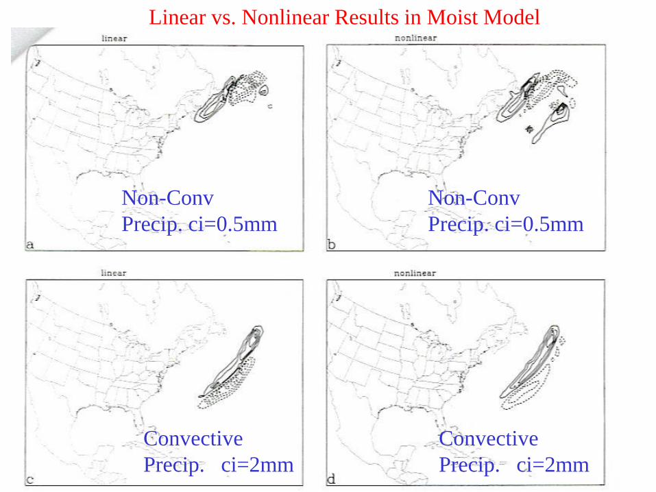
Non-Conv
Precip. ci=0.5mm
Convective
Precip. ci=2mm
Convective
Precip. ci=2mm
Non-Conv
Precip. ci=0.5mm
Linear vs. Nonlinear Results in Moist Model

Linear vs. Nonlinear Results
In general, agreement between TLM and NLM results
will depend on:
1. Amplitude of perturbations
2. Stability properties of the reference state
3. Structure of perturbations
4. Physics involved
5. Time period over which perturbation evolves
6. Measure of agreement
The agreement of the TLM and NLM is exactly
that of the Adjoint and NLM if the Adjoint is exact
with respect to the TLM.

Problems with Physics
1. The model may be non-differentiable.
2. Unrealistic discontinuities should be smoothed after
reconsideration of the physics being parameterized.
3. Perhaps worse than discontinuities are numerical insta-
bilities that can be created from physics linearization.
4. It is possible to test the suitability of physics components
for adjoint development before constructing the adjoint.
5. Development of an adjoint provides a fresh and
complementary look at parameterization schemes.

Efficient solution of optimization problems


M
Contours of J
in phase (x) space
P
Gradient
at point P
The more general nonlinear optimization problem
Find the local minima of a scalar nonlinear function J(x).

The Energy Norm

Problems with Physics

Tangent linear vs. nonlinear model solutions
Errico and
Raeder 1999
QJRMS
TLM
60x small pert NLM
NLM


Problems with Physics
Consider Parameterization of Stratiform Precipitation
R
0
qqs
NLM
TLM
TLM
Modified
NLM

Example of a potentially worse problem introduced by smoothing

Problems with Physics
1. The model may be non-differentiable.
2. Unrealistic discontinuities should be smoothed after
reconsideration of the physics being parameterized.
3. Perhaps worse than discontinuities are numerical insta-
bilities that can be created from physics linearization.
4. It is possible to test the suitability of physics components
for adjoint development before constructing the adjoint.
5. Development of an adjoint provides a fresh and
complementary look at parameterization schemes.
Other Important Considerations
Physically-based norms and the interpretations of
sensitivity fields

1 x 1.25 degree lat-lon 0.5 x 0.0625 degree lat-lon
∂ (error “energy”) / ∂ (Tv 24-hours earlier)
From R. Todling

Sensitivities of continuous fields

Sensitivity of J with respect to u 5 days earlier at 45ON,
where J is the zonal mean of zonal wind within a narrow
band centered on 10 hPa and 60ON. (From E. Novakovskaia)
10 hPa
0.1 hPa
1000 hPa
100 hPa
1 hPa
- 180 + 180 0 Longitude
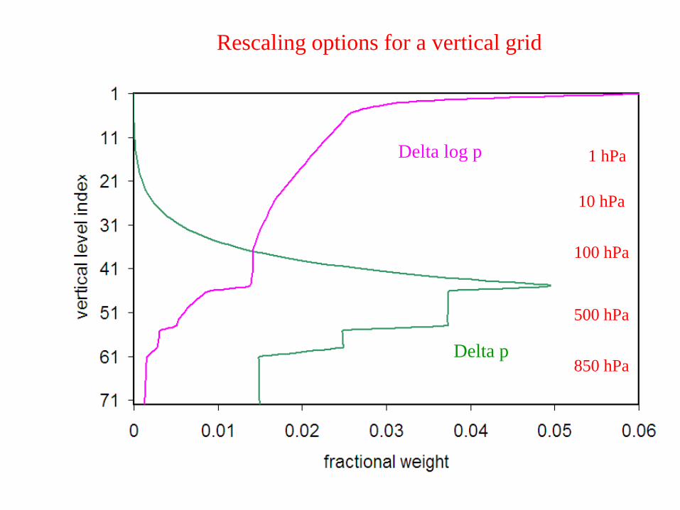
Rescaling options for a vertical grid
Delta log p
Delta p
500 hPa
100 hPa
10 hPa
1 hPa
850 hPa

1000
hPa
10
hPa
0.1
hPa
Mass weighting Volume weighting
2 Re-scalings of the adjoint results
From E. Novakovskaia

Summary

Misunderstanding #1
False: Adjoint models are difficult to understand.
True: Understanding of adjoints of numerical models
primarily requires concepts taught in early
college mathematics.

Misunderstanding #2
False: Adjoint models are difficult to develop.
True: Adjoint models of dynamical cores are simpler
to develop than their parent models, and almost
trivial to check, but adjoints of model physics
can pose difficult problems.

Misunderstanding #3
False: Automatic adjoint generators easily generate
perfect and useful adjoint models.
True: Problems can be encountered with automatically
generated adjoint codes that are inherent in the
parent model. Do these problems also have a
bad effect in the parent model?

Misunderstanding #4
False: An adjoint model is demonstrated useful and
correct if it reproduces nonlinear results for
ranges of very small perturbations.
True: To be truly useful, adjoint results must yield
good approximations to sensitivities with
respect to meaningfully large perturbations.
This must be part of the validation process.

Misunderstanding #5
False: Adjoints are not needed because the EnKF is
better than 4DVAR and adjoint results disagree
with our notions of atmospheric behavior.
True: Adjoint models are more useful than just for
4DVAR. Their results are sometimes profound,
but usually confirmable, thereby requiring new
theories of atmospheric behavior. It is rare that we
have a tool that can answer such important questions
so directly!

What is happening and where are we headed?
1. There are several adjoint models now, with varying
portions of physics and validation.
2. Utilization and development of adjoint models has been
slow to expand, for a variety of reasons.
3. Adjoint models are powerful tools that are under-utilized.
4. Adjoint models are like gold veins waiting to be mined.
5. Validity of some effects remains questionable.

Errico, R.M., 1997: What is an adjoint model. Bull. Am. Meteor. Soc., 78,
2577-2591.
Errico, R.M. and K.D. Raeder, 1999: An examination of the accuracy of the
linearization of a mesoscale model with moist physics. Quart. J. Roy. Met.
Soc., 125, 169-195.
Janisková, M., Mahfouf, J.-F., Morcrette, J.-J. and Chevallier, F., 2002:
Linearized radiation and cloud schemes in the ECMWF model:
Development and evaluation. Quart. J. Roy. Meteor. Soc.,128, 1505-1527
Papers by R. Gelaro, C. Reynolds, F. Rabier, M. Ehrendorfer, R. Langland,
M. Leutbecher, D. Holdaway
Adjoint Workshop series:
8th http://gmao.gsfc.nasa.gov/events/adjoint_workshop-8/
9th http://gmao.gsfc.nasa.gov/events/adjoint_workshop-9/
References