Embed Size (px)
Citation preview

Introduction to algebraic codingsLecture Notes for MTH 416
Fall 2012
Ulrich Meierfrankenfeld
December 7, 2012

2
PrefaceThese are the Lecture Notes for the class MTH 416 in Fall 2012 at Michigan State University.
The Lecture Notes will be frequently updated throughout the semester.

Contents
I Coding . . . . . . . . . . . . . . . . . . . . . . . . . . . . . . . . . . . . . . . . . . . . . . . . . . . . 5I.1 Matrices . . . . . . . . . . . . . . . . . . . . . . . . . . . . . . . . . . . . . . . . . . . . . . . 5I.2 Basic Definitions . . . . . . . . . . . . . . . . . . . . . . . . . . . . . . . . . . . . . . . . . . 8I.3 Coding for economy . . . . . . . . . . . . . . . . . . . . . . . . . . . . . . . . . . . . . . . . 9I.4 Coding for reliability . . . . . . . . . . . . . . . . . . . . . . . . . . . . . . . . . . . . . . . . 10I.5 Coding for security . . . . . . . . . . . . . . . . . . . . . . . . . . . . . . . . . . . . . . . . . 10
II Prefix-free codes . . . . . . . . . . . . . . . . . . . . . . . . . . . . . . . . . . . . . . . . . . . . . . 11II.1 The decoding problem . . . . . . . . . . . . . . . . . . . . . . . . . . . . . . . . . . . . . . . 11II.2 Representing codes by trees . . . . . . . . . . . . . . . . . . . . . . . . . . . . . . . . . . . . 13II.3 The Kraft-McMillan number . . . . . . . . . . . . . . . . . . . . . . . . . . . . . . . . . . . . 17II.4 A counting principal . . . . . . . . . . . . . . . . . . . . . . . . . . . . . . . . . . . . . . . . 19II.5 Unique decodability implies K ≤ 1 . . . . . . . . . . . . . . . . . . . . . . . . . . . . . . . . 20
III Economical coding . . . . . . . . . . . . . . . . . . . . . . . . . . . . . . . . . . . . . . . . . . . . . 23III.1 Probability distributions . . . . . . . . . . . . . . . . . . . . . . . . . . . . . . . . . . . . . . 23III.2 The optimization problem . . . . . . . . . . . . . . . . . . . . . . . . . . . . . . . . . . . . . 24III.3 Entropy . . . . . . . . . . . . . . . . . . . . . . . . . . . . . . . . . . . . . . . . . . . . . . . . 26III.4 Optimal codes – the fundamental theorems . . . . . . . . . . . . . . . . . . . . . . . . . . . . 28III.5 Hufman rules . . . . . . . . . . . . . . . . . . . . . . . . . . . . . . . . . . . . . . . . . . . . 31
IV Data Compression . . . . . . . . . . . . . . . . . . . . . . . . . . . . . . . . . . . . . . . . . . . . . 35IV.1 The Comparison Theorem . . . . . . . . . . . . . . . . . . . . . . . . . . . . . . . . . . . . . 35IV.2 Coding in pairs . . . . . . . . . . . . . . . . . . . . . . . . . . . . . . . . . . . . . . . . . . . 36IV.3 Coding in blocks . . . . . . . . . . . . . . . . . . . . . . . . . . . . . . . . . . . . . . . . . . 38IV.4 Memoryless Sources . . . . . . . . . . . . . . . . . . . . . . . . . . . . . . . . . . . . . . . . 40IV.5 Coding a stationary source . . . . . . . . . . . . . . . . . . . . . . . . . . . . . . . . . . . . . 41IV.6 Arithmetic codes . . . . . . . . . . . . . . . . . . . . . . . . . . . . . . . . . . . . . . . . . . 44IV.7 Coding with a dynamic dictionary . . . . . . . . . . . . . . . . . . . . . . . . . . . . . . . . . 47
V Noisy Channels . . . . . . . . . . . . . . . . . . . . . . . . . . . . . . . . . . . . . . . . . . . . . . . 51V.1 The definition of a channel . . . . . . . . . . . . . . . . . . . . . . . . . . . . . . . . . . . . . 51V.2 Transmitting a source through a channel . . . . . . . . . . . . . . . . . . . . . . . . . . . . . 53V.3 Conditional Entropy . . . . . . . . . . . . . . . . . . . . . . . . . . . . . . . . . . . . . . . . . 55V.4 Capacity of a channel . . . . . . . . . . . . . . . . . . . . . . . . . . . . . . . . . . . . . . . . 56
VI The noisy coding theorems . . . . . . . . . . . . . . . . . . . . . . . . . . . . . . . . . . . . . . . . 59VI.1 The probability of a mistake . . . . . . . . . . . . . . . . . . . . . . . . . . . . . . . . . . . . 59VI.2 Fano’s inequality . . . . . . . . . . . . . . . . . . . . . . . . . . . . . . . . . . . . . . . . . . 61VI.3 A lower bound for the probability of a mistake . . . . . . . . . . . . . . . . . . . . . . . . . 63VI.4 Extended Channels . . . . . . . . . . . . . . . . . . . . . . . . . . . . . . . . . . . . . . . . . 63VI.5 Coding at a given rate . . . . . . . . . . . . . . . . . . . . . . . . . . . . . . . . . . . . . . . . 67
3

4 CONTENTS
VI.6 Minimum Distance Decision Rule . . . . . . . . . . . . . . . . . . . . . . . . . . . . . . . . . 68VII Error Correcting . . . . . . . . . . . . . . . . . . . . . . . . . . . . . . . . . . . . . . . . . . . . . . 71
VII.1 Minimum Distance . . . . . . . . . . . . . . . . . . . . . . . . . . . . . . . . . . . . . . . . . 72VII.2 The Packing Bound . . . . . . . . . . . . . . . . . . . . . . . . . . . . . . . . . . . . . . . . . 74
VIII Linear Codes . . . . . . . . . . . . . . . . . . . . . . . . . . . . . . . . . . . . . . . . . . . . . . . . 79VIII.1 Introduction to linear codes . . . . . . . . . . . . . . . . . . . . . . . . . . . . . . . . . . . . 79VIII.2 Construction of linear codes using matrices . . . . . . . . . . . . . . . . . . . . . . . . . . . 81VIII.3 Standard form of check matrix . . . . . . . . . . . . . . . . . . . . . . . . . . . . . . . . . . . 83VIII.4 Constructing 1-error-correcting linear codes . . . . . . . . . . . . . . . . . . . . . . . . . . . 87VIII.5 Decoding linear codes . . . . . . . . . . . . . . . . . . . . . . . . . . . . . . . . . . . . . . . 90
IX Algebraic Coding Theory . . . . . . . . . . . . . . . . . . . . . . . . . . . . . . . . . . . . . . . . . 95IX.1 Classification and properties of cyclic codes . . . . . . . . . . . . . . . . . . . . . . . . . . . 95IX.2 Definition of a family of BCH codes . . . . . . . . . . . . . . . . . . . . . . . . . . . . . . . 107IX.3 Properties of BCH codes . . . . . . . . . . . . . . . . . . . . . . . . . . . . . . . . . . . . . . 112
X Cryptography in theory and practice . . . . . . . . . . . . . . . . . . . . . . . . . . . . . . . . . . . 117X.1 Encryption in terms of a channel . . . . . . . . . . . . . . . . . . . . . . . . . . . . . . . . . 117X.2 Perfect secrecy . . . . . . . . . . . . . . . . . . . . . . . . . . . . . . . . . . . . . . . . . . . . 119X.3 The one-time pad . . . . . . . . . . . . . . . . . . . . . . . . . . . . . . . . . . . . . . . . . . 120X.4 Iterative methods . . . . . . . . . . . . . . . . . . . . . . . . . . . . . . . . . . . . . . . . . . 121X.5 The Double-Locking Procedure . . . . . . . . . . . . . . . . . . . . . . . . . . . . . . . . . . 122
XI The RSA cryptosystem . . . . . . . . . . . . . . . . . . . . . . . . . . . . . . . . . . . . . . . . . . 125XI.1 Public-key cryptosytems . . . . . . . . . . . . . . . . . . . . . . . . . . . . . . . . . . . . . . 125XI.2 The Euclidean Algorithim . . . . . . . . . . . . . . . . . . . . . . . . . . . . . . . . . . . . . 125XI.3 Definition of the RSA public-key cryptosystem . . . . . . . . . . . . . . . . . . . . . . . . . 128
A Rings and Field . . . . . . . . . . . . . . . . . . . . . . . . . . . . . . . . . . . . . . . . . . . . . . . 131A.1 Basic Properties of Rings and Fields . . . . . . . . . . . . . . . . . . . . . . . . . . . . . . . 131A.2 Polynomials . . . . . . . . . . . . . . . . . . . . . . . . . . . . . . . . . . . . . . . . . . . . . 133A.3 Irreducible Polynomials . . . . . . . . . . . . . . . . . . . . . . . . . . . . . . . . . . . . . . 135A.4 Primitive elements in finite field . . . . . . . . . . . . . . . . . . . . . . . . . . . . . . . . . . 136
B Constructing Sources . . . . . . . . . . . . . . . . . . . . . . . . . . . . . . . . . . . . . . . . . . . . 141B.1 Marginal Distributions on Triples . . . . . . . . . . . . . . . . . . . . . . . . . . . . . . . . . 141B.2 A stationary source which is not memory less . . . . . . . . . . . . . . . . . . . . . . . . . . 142B.3 Matrices with given Margin . . . . . . . . . . . . . . . . . . . . . . . . . . . . . . . . . . . . 142
C More On channels . . . . . . . . . . . . . . . . . . . . . . . . . . . . . . . . . . . . . . . . . . . . . 145C.1 Sub channels . . . . . . . . . . . . . . . . . . . . . . . . . . . . . . . . . . . . . . . . . . . . . 145
D Examples of codes . . . . . . . . . . . . . . . . . . . . . . . . . . . . . . . . . . . . . . . . . . . . . 147D.1 A 1-error correcting binary code of length 8 and size 20 . . . . . . . . . . . . . . . . . . . . 147

Chapter I
Coding
I.1 MatricesDefinition I.1. Let I and R be sets.
(a) An I-tuple with coefficients in R is a function x ∶ I → R. We will write xi for the image of i under x anddenote x by (xi)i∈I . xi is called the i-coefficient of x.
(b) Let n ∈ N, where N = 0,1,2,3, . . . , denotes the set of non-negative integers. Then an n-tuple is an1,2, . . . ,n-tuple.
Notation I.2. Notation for tuples.
1.
x ∶a b c d
0 π 1 13
denotes a,b, c,d-tuple with coefficients in R such that
xa = 0, xb = π, xc = 1 and xd =13
We denote this tuple also by
x ∶
a 0
b π
c 1
d 13
2.y = (a,a,b, c)
denotes the 4-tuple with coefficients in a,b, c,d, e, . . . , z such that
y1 = a, y2 = a, y3 = b and y4 = c
5

6 CHAPTER I. CODING
We will denote such a 4-tuple also by
y =
⎛⎜⎜⎜⎜⎜⎜⎜⎜⎝
a
a
b
c
⎞⎟⎟⎟⎟⎟⎟⎟⎟⎠
Definition I.3. Let I, J and R be sets.
(a) An I × J-matrix with coefficients in R is a function M ∶ I × J → R. We will write mi j for the image of (i, j)under M and denote M by [mi j] i∈I
j∈J. mi j is called the i j-coefficients of M.
(b) Let n.m ∈ N. Then an n ×m-matrix is an 1,2, . . . ,n × 1,2, . . . ,m-matrix.
Notation I.4. Notations for matrices
1. We will often write an I × J-matrix as an array. For example
M x y z
a 0 1 2
b 1 2 3
c 2 3 4
d 3 4 5
stands for the a,b, c,d × x, y, z matrix M with coefficients in Z such that max = 0, may = 1, mbx = 1,mcz = 4, . . . .
2. n ×m-matrices are denoted by an n ×m-array in square brackets. For example
M =⎡⎢⎢⎢⎢⎢⎣
0 1 2
4 5 6
⎤⎥⎥⎥⎥⎥⎦denotes the 2 × 3 matrix M with m11 = 0,m12 = 2, m21 = 4, m23 = 6,. . . .
Definition I.5. Let M be an I × J-matrix.
(a) Let i ∈ I. Then row i of M is the J-tuple (mi j) j∈J . We denote row i of M by Rowi(M) or by Mi.
(b) Let j ∈ J. Then column j of J is the I-tuple (mi j)i∈I . We denote column j of M by Col j(M)
Definition I.6. Let A be I × J-matrix, B an J ×K matrix and x and y J-tuples with coefficients in R. SupposeJ is finite.
(a) AB denotes the I × K matrix whose ik-coefficient is
∑j∈J
ai jb jk

I.1. MATRICES 7
(b) Ax denotes the I-tuple whose i-coefficient is
∑j∈J
ai jx j
(c) xB denotes the K-tuple whose k-coefficient is
∑j∈J
x jb jk
(d) xy denotes the real number
∑j∈J
x jy j
Example I.7. Examples of matrix multiplication.
1. Given the matrices
A x y z
a 0 1 2
b 1 2 3
and
B α β γ δ
x 0 0 1 0
y 1 0 0 1
x 1 1 0 0
Then AB is the a,b × α, β, γ, δ matrix
AB α β γ δ
a 3 2 0 1
b 4 c 1 2
2. Given the matrix 2 × 3-matrix A =⎡⎢⎢⎢⎢⎢⎣
0 1 2
1 2 3
⎤⎥⎥⎥⎥⎥⎦and the 3-tuple x =
⎛⎜⎜⎜⎜⎝
0
1
1
⎞⎟⎟⎟⎟⎠
Then
Then Ax is the 2-tuple
⎛⎜⎝
3
5
⎞⎟⎠
3. Since we may represent tuples also as rows, (2) can be restated as:
Given the matrix 2 × 3-matrix A =⎡⎢⎢⎢⎢⎢⎣
0 1 2
1 2 3
⎤⎥⎥⎥⎥⎥⎦and the 3-tuple x = (0,1,1). Then
Then Ax is the 2-tuple
(3,5)

8 CHAPTER I. CODING
4. Given the matrix
A x y z
a 0 1 2
b 1 2 3
and the tuple u ∶a b
2 −1
Then uA is the x, y, z-tuple
x y z
−1 0 1
5. Given the 4-tuples x = (1,1,2,−1) and y = (−1,1,2,1). Then
xy = 3
I.2 Basic DefinitionsDefinition I.8. An alphabet is a finite set. The elements of an alphabet are called symbols.
Example I.9. (a) A = A,B,C,D, . . . ,X,Y,Z,⊔ is the alphabet consisting of the regular 27 uppercase lettersand a space (denoted by ⊔).
(b) B = 0,1 is the alphabet consisting of the two symbols 0 and 1
Definition I.10. Let S be an alphabet and n a non-negative integer.
(a) A message of length n in S is an n-tuple (s1, . . . , sn) with coefficients in S . We denote such an n-tuple bys1s2 . . . sn. A message of length n is sometimes also called a string of length n.
(b) ∅ denote the unique message of length 0 in S .
(c) S n is the set of all messages of length n in S .
(d) S ∗ is the set of all messages in S , so
S ∗ = S 0 ∪ S 1 ∪ S 2 ∪ S 3 ∪ . . . ∪ S k ∪ . . .
Example I.11. 1. ROOM⊔C206WH⊔IS⊔NOW⊔A216WH is a message in the alphabet A.
2. 1001110111011001 is a message in the alphabet B.
3. B0 = ∅, B1 = B = 0,1. B2 = 00,01,10,11, B3 = 000,001,010,011.100,101,110,111, and
B∗ = ∅,0,1,00,01,10,11,000, . . . ,111,0000. . . . ,1111, . . .
Definition I.12. Let S and T be alphabets.
(a) A code c for S using T is a 1-1 function from S to T∗. So a code assigns to each symbol s ∈ S a messagec(s) in T , and different symbols are assigned different messages
(b) The set C = c(s) ∣ s ∈ S is called the set of codewords of c. Often (somewhat ambiguously) we willalso call C a code. To avoid confusion, a code which is function will always be denoted by a lower caseletter, while a code which is a set of codewords will be denoted by an upper case letter.

I.3. CODING FOR ECONOMY 9
(c) A code is called regular if the empty message ∅ is not a codeword.
Example I.13. 1. The function c ∶ A→ A such that
A→ D,B→ E,C → F, . . . ,W → Z,X → A,Y → B,Z → C,⊔→ ⊔
is a code for A using A. The set of codewords is C = A.
2. The function c ∶ x, y, z→ B∗ such that
x→ 0, y→ 01, z→ 10
is a code for x, y, z using B. The set of codewords is C = 0,01,10.
Definition I.14. Let c ∶ S → T∗ be a code. Then the function c∗ ∶ S ∗ → T∗ defined by
c∗(s1s2 . . . sn) = c(s1)c(s2) . . . c(sn)
for all s1 . . . sn ∈ S ∗ is called the concatenation of c. We also call c∗ the extension of c. Often we will denotec∗ by c rather than c. Since c is uniquely determined by c∗ and vice versa, this ambiguous notation shouldnot lead to any confusion.
Example I.15. 1. Let c ∶ A→ A∗ be the code from I.13(1). Then c(MTH)=PWK.
2. Let c ∶ x, y, z→ B∗ be the code from I.13(2). Then c(xzzx) = 010100 and c(yyxx) = 010100.
So xzzx and yxx are encoded to the same message in B.
Definition I.16. A code c ∶ S → T∗ is called uniquely decodable (UD) if the extended function c ∶ S ∗ → T∗
is 1-1.
Example I.17. (a) The code from I.15(1) is UD.
(b) The code from I.15(2) is not UD.
I.3 Coding for economy
Example I.18. The Morse Alphabet M has three symbols ,− and ⊙, called dot, dash and pause. The Morsecode is the code for A using M defined by
A B C D E F G H I
− ⊙ − ⊙ − − ⊙ − ⊙ ⊙ − ⊙ − − ⊙ ⊙ ⊙
J K L M N 0 P Q R
− − − ⊙ − −⊙ − ⊙ − − ⊙ − ⊙ − − − − − ⊙ − − − ⊙ − ⊙
S T U V W X Y Z ⊔
⊙ −⊙ −⊙ − ⊙ − −⊙ − − ⊙ − − − ⊙ − − ⊙⊙

10 CHAPTER I. CODING
I.4 Coding for reliabilityExample I.19. Codes for Buy,Sell using B,S .
1. Buy→ B, Sell→ S.
2. Buy→ BB, Sell→ SS.
3. Buy→ BBB, Sell→ SSS.
4. Buy→ BBBBBBBBB, Sell→ SSSSSSSSS.
I.5 Coding for securityExample I.20. Let k be an integer with 0 ≤ k ≤ 25. Then ck is the code from A→ A obtained by shifting eachletter by k-places. ⊔ is unchanged. For example the code in I.13(1), is c3.
This code is not very secure, in the sense that given an encoded message it is not very difficult to todetermine the original message (even if one does not know what parameter was used).

Chapter II
Prefix-free codes
II.1 The decoding problemDefinition II.1. Let C be a code using the alphabet T .
(a) Let a,b ∈ T∗. Then a is called a prefix of b if there exists a message r in T∗ with b = ar.
(b) Let a,b ∈ T∗. Then a is called a parent of b if there exists r ∈ T with b = ar.
(c) C is called prefix-free (PF) if no codeword is a prefix of a different codeword.
Remark II.2. T be an alphabet and b = t1 . . . tm a message of length m in T .
(a) Any prefix of b has length less or equal to m.
(b) Let 0 ≤ n ≤ m. Then t1 . . . tn is the unique prefix of length n of b.
(c) If m ≠ 0, then t1 . . . tm−1 is the unique parent of b.
Proof. Let a = s1 . . . sn be a prefix of length n of b. Then b = ar for some r ∈ T∗ or length say k. Letr = u1 . . .uk. Then b = s1 . . . snu1 . . .uk. Thus m = n + k and n ≤ m and (a) holds. Also ti = si for 1 ≤ i ≤ n andso a = t1 . . . tn and (b) holds. If a is a parent then r ∈ T , that is k = 1 and n = m−1. So (c) follows from (a).
Example II.3. Which of the following codes are PF? UD?
1. Let C = 10,01,11,011. Since 01 is a prefix of 011, C is not prefix-free. Also
011011 = (01)(10)(11) = (011)(011)
and so C is not uniquely decodable.
2. Let C = 021,2110,10001,21110. Observe that C is prefix free.
This can be used to recover the sequence c1, c2 . . . , cn of codewords from their concatenation e = c1 . . . cn.Consider for example the string
e = 2111002110001
We will look at prefixes of increasing length until we find a codeword:
11
12 CHAPTER II. PREFIX-FREE CODES
Prefix codeword?
∅ no
2 no
21 no
211 no
2111 no
21110 yes
No longer prefix can be a codeword since it would have the codeword 21110 as a prefix.
So c1 = 21110.
We now remove 21110 from e to get
02110001
The prefixes are
Prefix codeword?
∅ no
0 no
02 no
021 yes
So c2 = 021. Removing 021 gives
10001
This is a codeword and so c3 = 10001. Thus the only decomposition of e into codewords is
2111002110001 = (21110)(021)(1001)
This example indicates that C is UD. The next theorem confirms this
Theorem II.4. Any regular PF code is UD.
Proof. Let n,m ∈ N and c1, . . . , cn, d1, . . . ,dm be codewords with
c1 . . . cn = d1 . . .dm
We need to show that n = m and c1 = d1, c2 = d2, . . . , cn = dn. The proof is by complete induction on n+m.Put e = c1 . . . cn and so also e = d1 . . .dm.
Suppose first that n = 0. Then e = ∅ and so d1 . . .dm = ∅, By definition of a regular code each di is notempty. Hence also m = 0 and we are done in this case.

II.2. REPRESENTING CODES BY TREES 13
So we may assume that n > 0 and similarly m > 0. Let k and l be the lengths of c1 and d1 respectively.We may assume that k ≤ l. Since e = c1 . . . cn, c1 is the prefix of length k of e. Also e = d1 . . .dm implies
that d1 is the prefix of length l of e. Since k ≤ l this shows that c1 is the prefix of length k of d1. Since C isprefix free we conclude that c1 = d1. Since c1c2 . . . cn = d1d2 . . .dm this implies
c2 . . . cn = d2 . . .dm
From the induction assumption we conclude that n − 1 = m − 1 and c2 = d2, . . . , cn = dm.
Lemma II.5. (a) All UD codes are regular.
(b) Let c ∶ S → T∗ be not regular. Then c is PF if and only if ∣S ∣ = 1 and c(s) = ∅ for s ∈ C.
Proof. Let c ∶ S → T∗ be non-regular code. Then there exists s ∈ S with c(s) = ∅ for s ∈ S . Thus
c∗(ss) = ∅∅ = ∅ = c∗(s).
and so c is not UD and (a) holds.
If ∣S ∣ > 1, then c has at least two codewords. Since c(s) = ∅ is the prefix of any message we concludethat S is not PF. This proves the forward direction in (b).
Any code with only one codeword is PF and so the backwards direction in (b) holds.
II.2 Representing codes by treesDefinition II.6. A graph G is a pair (V,E) such that V and E are sets and each elements e of E is a subsetof size two of V. The elements of V are called the vertices of V. The elements of E are called the edges of V.We say that the vertex a is adjacent to b in G if a,b is an edge.
Example II.7. Let V = 1,2,3,4 and E = 1,2,1,3,1,4,2,3,3,4. Then G = (V,E) is a graph
It is customary to represent a graph by a picture: Each vertex is represented by a node and a line is drawnbetween any two adjacent vertices. For example the above graph can be visualized by the following picture:
1 2
4 3
Definition II.8. Let G = (V,E) be a graph.
(a) Let a and b be vertices. A path of length n from a to b in G is a tuple (v0, v1, . . . , vn) of vertices such thata = v0, b = vn and vi−1 is adjacent to vi for all 1 ≤ i ≤ n.
(b) G is called connected if for each a,b ∈ G, there exists a path from a to b in G.
(c) A path is called a cycle if the first and the last vertex are the same.
(d) A cycle is called simple if all the vertices except the last one are pairwise distinct.

14 CHAPTER II. PREFIX-FREE CODES
(e) A tree is a connected graph with no simple cycles of length larger than two.
Example II.9. Which of the following graphs are trees?
1.
1 2
4 3
is connect, but
1 2
3
is simple circle of length three in G. So G is not a tree.
2.
1 2
4 3
has no simple circle of length larger than two. But it is not connected since there is no path from 1 to 2.So G is not a tree.
3.
1 2
4 3
5
6

II.2. REPRESENTING CODES BY TREES 15
is connected and has no simple circle of length larger than two. So it is a tree.
Example II.10. The infinite binary tree
How can one describe this graph in terms of pair (V,E)?. The vertices are binary messages and a messagea is adjacent to message b if a is the parent of b or b is the parent of a.
V = B∗ and E = a,as∣a ∈ β∗, s ∈ B = a,b∣a,b ∈ B∗,a is the parent of b
So the infinite binary tree now looks like:
010 011 100 101 110 111
16 CHAPTER II. PREFIX-FREE CODES
Definition II.11. Let C be a code. Then G(C) is the graph (V,E), where V is the set of prefixes of codewordsand
E = a,b∣a,b ∈ V,a is a parent of b
G(C) is called the graph associated to C.
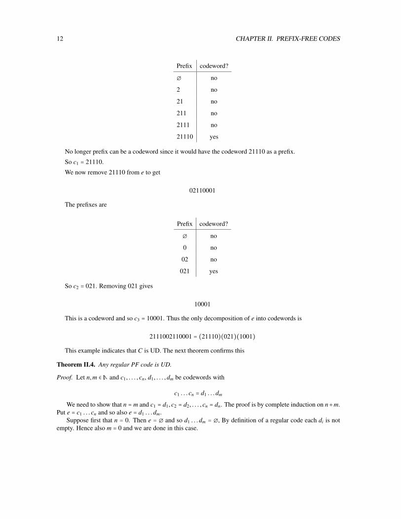
Example II.12. Determine the tree associated to the code C = 0,10,110,111.
0
10
110 111
Definition II.13. Let G be a tree. A leave of G is a vertex which is adjacent to at most one vertex of G.
Theorem II.14. Let C be a code and let G(C) = (V,E) be the graph associate to C.
(a) Let c ∈ V be of length n. For 0 ≤ k ≤ n let ck be the prefix of length k of c. Then (c0, c1, . . . , cn) is a pathfrom ∅ to c in G(C).
(b) G(C) is tree.
(c) Let c be a codeword. Then c is prefix of another codeword if and only if c is adjacent to at least twovertices of G(C).
(d) C is prefix-free if and only if all codewords of C are leaves of G(C).
Proof. (a) Just observe that ci = ci−1ti where ti is the i-symbol of c. Hence ci−1 is adjacent to ci and (c0, . . . , cn)is a path. Also c0 = ∅ and cn = c.
(b) By (a) there exists a path from each vertex of G(C) to ∅. It follows that G is connected.We prove next:
1. Let (a0,a1 . . . ,am) be path in G(C) with pairwise distinct vertices of length at least 1. Let li be lengthof ai and suppose that l0 ≤ l1. Then for all 1 ≤ i ≤ m, ai−1 is the parent of ai. In particular, li = l0 + i for all0 ≤ i ≤ m and ai is a prefix of a j for all 0 ≤ i ≤ j ≤ m.
Since a0 is adjacent to a1, either one of a0 and a1 is the parent of the other. Since l0 ≤ l1 we conclude thata0 is parent of a1. So if m = 1, (1) holds. Suppose m ≥ 2. Since a2 ≠ a0 and a0 is the parent of a1, a2 isnot the parent of a1. Since a2 is adjacent to a1 we conclude that a1 is the parent of a2. In particular, l1 ≤ l2.Induction applied to the path (a1, . . . ,am) shows that ai−1 is a parent of ai for all 2 ≤ i ≤ m and so the firststatement inrf 1 is proved.
The remaining statements follow from the first.
Now suppose for a contradiction that there exists a simple circle (v0, v1, . . . , vn) in G(C) with n ≥ 3. Letl = min0≤i≤n l(vi) and choose 0 ≤ k ≤ n such that l(vk) = l.
Assume that 0 < k < n. Then we can apply (1) to the paths (vk, . . . , vn) and (vk, vk−1, . . . v0). It followsthat vk+1 is the prefix of length l + 1 of vn and vk−1 is the prefix of length l + 1 of v0. Since (v0, . . . , vn) is a

II.3. THE KRAFT-MCMILLAN NUMBER 17
circle we have v0 = vn and we conclude that vk−1 = vk+1. Thus implies k − 1 = 0 and k + 1 = n. So n = 2, acontradiction.
Assume next that k = 0 or k = n. Since v0 = vn we conclude that v0 and vn have length l. By (1) appliedto (v0, v1), v1 has length l+1 and by (1) applied to (vn, vn−1, . . . , v1). v1 has length l+ (n−1). Thus n−1 = 1and again n = 2.
So G(C) has no simple circle of length at least three. We already proved that G(C) is connected and soG(C) is a tree.
(c): Suppose first that a,b are distinct codewords and a is the prefix of b. Let l = l(a). Let c be the prefixof length l + 1 of b. Then a is the parent of c. Since c is prefix of the codeword b, c ∈ V . So c is adjacent toa. By definition of a code, a ≠ ∅ and so a has a parent d. Then d is in V , d is adjacent to a and d ≠ c. So a isadjacent to at least two distinct vertices of G(C).
Suppose next that a is a codeword and a is adjacent to two distinct vertices c and d in V . One of c and d,say c is not the parent of a. Since a is adjacent to c, this means that a is a parent of c. Since c is a V , c is theprefix of some codeword b. Since a is the parent of c, a is a prefix of b and a ≠ b. So a is the prefix of anothercodeword.
(d) C is prefix free if and only if no codeword is a prefix of another codeword and so by (a) if and onlyif no codewords is adjacent two different vertices of G(C), that is very codewords is adjacent to at most onevertex and so if and only if each codeword is a leave.
II.3 The Kraft-McMillan numberDefinition II.15. Let C be a code using the alphabet T .
(a) C is called a b-ary code, where b = ∣T ∣.
(b) Let i be a non-negative integer. Then Ci is the set of codewords of length i and ni = ∣Ci∣. So ni is thenumber of codewords of length i.
(c) Let M be the maximal length of a codeword. (So nM ≠ 0 and ni = 0 for all i > M). The M-tuple n =(n0,n1, . . . ,nM) is called the parameter of C. More generally if N ≥ M we will also call (n0,n1, . . . ,nN)the parameter of C.
(d) The number
K ∶=M
∑i=0
ni
bi= n0 +
n1
b+ n2
b2+ . . . + nM
bM
is called the Kraft-McMillan number associated to the parameter (n0,n1, . . . ,nM) and the base b, andalso is called the Kraft-McMillan number of C.
Example II.16. Compute the Kraft-McMillan number of the binary code C = 10,01,11,011.
We have C0 = , C1 = , C2 = 10,01,11 and C3 = 011. So the parameter is (0,0,3,1) and
K = 0 + 02+ 3
4+ 1
8= 6 + 1
8= 7
8Lemma II.17. Let C be a code with Kraft-MacMillan number K using the alphabet T . Let M be a positiveinteger such that every code word has length less than N. Let D be the set message of length M in T whichhave a codeword as a prefix. Then

18 CHAPTER II. PREFIX-FREE CODES
(a) ∣D∣ ≤ KbM .
(b) If C is PF, ∣D∣ = bMK.
(c) If C is PF, then K ≤ 1.
Proof. (a) Let c be a codeword of length i. Then any message of length M in T is of the from cr where r isa message of length M − i. Note that where are bM−i such messages and so there are exactly bM−i message oflength M which have c as a prefix. It follows that there are at most nibM−i message of length M which have acodeword of length i as a prefix. Thus
∣D∣ ≤M
∑i=0
nibM−i = bmM
∑i=1
nib−i = bMK
(b) Suppose C is prefix-free. Then a message of length M can have at most one codeword as a prefix. Sothe estimate in (a) is exact.
(c) Note that the numbers of message of length M is bM . Thus ∣D∣ ≤ bM and so by (b), bMK ≤ bM . HenceK ≤ 1.
Theorem II.18. Let b and M be integers with M ≥ 0 and b ≥ 1. Let n = (n0,n1, . . . ,nM) be tuple of non-negative integers such that K ≤ 1, where K is the Kraft-McMillan number associated to parameter n and thebase b. Then there exists a b-ary PF code C with parameter n.
Proof. The proof is by induction on M. Let T be any set of b-elements.Suppose first that M = 0. Then n0 = K ≤ 1. If n0 = 0 let C = and if n0 = 1 let C = ∅. Then C is a PF
code with parameter n = (n0).Suppose next that M ≥ 1 and that the theorem holds for M − 1 in place of M.Put K = ∑M−1
i=0nibi . Then
K + nM
bM= K ≤ 1
and so
(∗) K = K − nM
bM≤ 1 − nM
bM≤ 1
By the induction assumption there exists a PF code C with parameter (n0,n1, . . . ,nM−1). Let D be the setof messages of length M in T which have a codeword from C as a prefix. By II.17 ∣D∣ = bM K. Multiplying(*) with bM gives bM K ≤ bM − nM . Thus ∣D∣ ≤ bM − nm and so nm ≤ bM − ∣D∣. Since bM is the number ofmessages of length bM , bM − ∣D∣ is the number of messages of length M which do not have a codeword as aprefix. Thus there exists a set D of message of length M such that ∣D∣ = nM and none of the messages has acodeword from C as a prefix. Put C = C ∪ D.
We claim that C is prefix-free. For this let a and b be distinct elements of C.Suppose that a and b are both in C. Since C is PF, a is not a prefix of b.Suppose that a and b are both in D. Thena and b have the same length and so a is not a prefix of b.Suppose that a ∈ C and b ∈ D. Then the choice of D shows that a is not a prefix of b.Suppose that a ∈ D and b ∈ C. a has larger length than b and so again a is not a prefix of b.Thus C is indeed PF.If a is a codeword of length i with i < M, then a is one of the ni codewords of C of length i. If a is a
codeword of length at least M, then a is one of the nm-codewords in D and a has length M. Thus the parameterof C are (n0,n1, . . . ,nM−1,nM) and so C has all the required properties.
II.4. A COUNTING PRINCIPAL 19
II.4 A counting principalLemma II.19. Let c ∶ S → T∗ and d ∶ R→ T∗ be codes. Define the function cd ∶ S × R→ T∗ by
(cd)(s, r) = c(s)d(r)
for all s ∈ S , r ∈ R. Also let C and D be the set of codewords of c and d, respectively, and define
CD = ab ∣ a ∈ C,b ∈ D
Then cd is a code if and only for each e ∈ CD, there exists unique a ∈ C and b ∈ D with e = cd. In thiscase CD is set of codewords of cd.
Proof. Let s ∈ S and r ∈ R. Since c is a code, c(s) is not the empty message and so also c(s)d(r) is not theempty message. Hence (cd)(r, s) ≠ ∅ for all (s, r) ∈ S × R.
Thus cd is a code if and only of cd is 1-1. We have
Im cd = (cd)(s, r)∣ (s, r) ∈ S × R = c(s)d(r)∣ s ∈ S , r ∈ R = ab∣a ∈ C,d ∈ D = CD
In particular, CD is the set of codewords of cd.Moreover, cd is 1-1 if and only if for each e ∈ CD there unique s ∈ S and r ∈ R with e = c(s)d(r). Since
c and d are 1-1, this holds if and only if for each e ∈ CD there exist unique a ∈ C and b ∈ D with e = ab.
Definition II.20. Let C be a code with parameter (n0,n1, . . . ,nM). Then
QC(x) = n0 + n1x + n2x2 + . . . + nM xm
is called the generating function of c.
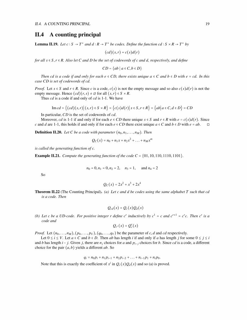
Example II.21. Compute the generating function of the code C = 01,10,110,1110,1101.
n0 = 0,n1 = 0,n2 = 2, n3 = 1, and n4 = 2
So
QC(x) = 2x2 + x3 + 2x4
Theorem II.22 (The Counting Principal). (a) Let c and d be codes using the same alphabet T such that cdis a code. Then
Qcd(x) = Qc(x)Qd(x)
(b) Let c be a UD-code. For positive integer r define cr inductively by c1 = c and cr+1 = crc. Then cr is acode and
Qcr(x) = Qrc(x)
Proof. Let (n0, . . . ,nM), (p0, . . . , pU), (q0, . . . ,qV) be the parameter of c,d and cd respectively.Let 0 ≤ i ≤ V . Let a ∈ C and b ∈ D. Then ab has length i if and only if a has length j for some 0 ≤ j ≤ i
and b has length i− j. Given j, there are n j choices for a and pi− j choices for b. Since cd is a code, a differentchoice for the pair (a,b) yields a different ab. So
qi = n0 pi + n1 pi−1 + n2 pi−2 + . . . + ni−1 p1 + ni p0.
Note that this is exactly the coefficient of xi in Qc(x)Qd(x) and so (a) is proved.

20 CHAPTER II. PREFIX-FREE CODES
Since c is a UD code the extended function c∗ ∶ S ∗ → T∗ is 1-1. Observe that cr is just the restriction of c∗ toS r. So also cr is 1-1 and thus cr is a code. Applying (a) r − 1 times gives
Qcr(x) = Q cc...c±r−times
(x) = Qc(x)Qc(x) . . .Qc(x)´¹¹¹¹¹¹¹¹¹¹¹¹¹¹¹¹¹¹¹¹¹¹¹¹¹¹¹¹¹¹¹¹¹¹¹¹¹¹¹¹¹¹¹¹¹¹¹¹¹¹¹¹¹¹¹¹¹¹¹¹¹¸¹¹¹¹¹¹¹¹¹¹¹¹¹¹¹¹¹¹¹¹¹¹¹¹¹¹¹¹¹¹¹¹¹¹¹¹¹¹¹¹¹¹¹¹¹¹¹¹¹¹¹¹¹¹¹¹¹¹¹¹
r−times
= Qrc(x).
II.5 Unique decodability implies K ≤ 1
Lemma II.23. Let c be a b-ary code with maximal codeword length M and Kraft McMillan number K. Then
(a) K ≤ M + 1 and if c is regular, K ≤ M.
(b) K = Qc ( 1b).
Proof. (a) Since there are bi messages of length i, ni ≤ bi and nibi≤ 1. So each summand in the Kraft McMillan
number is bounded by 1. Note that there are M + 1 summand and so K ≤ M + 1. If c is regular, ∅ is not acodeword and n0 = 0. So K ≤ M in this case.
(b)
K =M
∑i=0
n0
bi=
M
∑i=0
ni (1b)
i
= Qc (1b)
Lemma II.24. (a) Let c ∶ S → T∗ and d ∶ R → T∗ be codes such that cd is a code. Let K and L be the KraftMcMillan number of c and d, respectively. Then KL is the Kraft McMillan number of cd.
(b) Let c be a UD-code with Kraft McMillan number K. Then the Kraft McMillan number of cr is Kr.
Proof. (a) The Kraft McMillan number of cd is
Qcd (1b) = Qc (
1b) Qd (
1b) = KL
(b) follows from (a) and induction.
Theorem II.25. Let C be a UD-code with Kraft McMillan number K. Then K ≤ 1.
Proof. Let M be the maximal codeword length of C. Then the maximal codeword length of Cr is rM and -byII.24(b) - the Kraft McMillan number of Cr is Kr. By II.23 the Kraft-McMillan number is bounded by themaximal codeword length plus 1 and so
Kn ≤ rM + 1
for all r ∈ Z+. Thus
r ln K ≤ ln(rM + 1) and ln K ≤ ln (rM + 1)r
The derivative of x is 1 and of ln(xM + 1) is MxM+1 . L’Hopital’s Rule gives
limr→∞
ln(rM)r
= limr→∞
MrM+1
1= 0
and so ln K ≤ 0 and K ≤ 1.

II.5. UNIQUE DECODABILITY IMPLIES K ≤ 1 21
Corollary II.26. Given a parameter (n0, . . . ,nM) and a base b with Kraft-McMillan number K. Then thefollowing statements are equivalent.
(a) Either ∣S ∣ = 1 and (n0, . . . ,nM) = (1,0, . . . ,0), or there exists a b-ary UD code with parameter (n0, . . . ,nM).
(b) K ≤ 1.
(c) There exists a b-ary PF code with parameter (n0, . . . ,nM).
Proof. By II.25, (a) implies (b). By II.18 (b) implies (c). Suppose c is a b-ary PF-code with parameter(n0, . . . ,nM). If c is regular, II.4 shows that c is UD and (a) holds. If c is not regular, then ∅ is a codewordand since c is prefix free, ∅ is the only codeword. So the parameter of c is (1,0, . . . ,0) and again (a) holds.

22 CHAPTER II. PREFIX-FREE CODES

Chapter III
Economical coding
III.1 Probability distributionsDefinition III.1. Let S be an alphabet. Then a probabilty distribution on S is an S -tuple with coefficients inthe interval [0,1] such that
∑s∈S
ps = 1
Notation III.2. Suppose S is an alphabet with exactly m-symbols s1, s2, . . . , sm and that
t ∶s1 s2 . . . sm
t1 t2 . . . tm
is an S -tuple.Then we will denote t by (t1, . . . , tm). Note that this is slightly ambiguous, since t does not only depended
on the n-tuple (t1, . . . , tm) but also on the order of the elements s1, . . . , sm.
Example III.3.
(a)
p ∶w x y z12
13 0 1
6
is a probability distribution on w, x, y, z.
(b) Using the notation from III.2 Example (b) can be stated as: p = ( 12 ,
13 ,0,
16) is a probability distribution
on w, x, y, z. Note that px = 13 .
(c) p = ( 12 ,
13 ,0,
16) is a probability distribution on x,w, z, y. Note that px = 1
2 .
(d)
A B C D E F G H I
8.167% 1.492% 2.782% 4.253% 12.702% 2.228% 2.015% 6.094% 6.966%
23

24 CHAPTER III. ECONOMICAL CODING
J K L M N O P Q R
0.153% 0.747% 4.025% 2.406% 6.749% 7.507% 1.929% 0.095% 5.987%
S T U V W X Y Z ⊔
6.327% 9.056% 2.758% 1.037% 2.365% 0.150% 1.974% 0.074% 0
is a probability distribution on A. It lists how frequently a letter is used in the English language.
(e) Let S be a set with m elements and put p = ( 1m)
s∈S. Then ps = 1
m for all s ∈ S and p is probabilitydistribution on S . p is called the equal probability distribution on S .
III.2 The optimization problemDefinition III.4. Let c ∶ S → T∗ be a code and p a probability distribution on S .
(a) For s ∈ S let ys be length of the codeword c(s). The S -tuple y = (ys)s∈S is called the codeword length ofc.
(b) The average length codeword length of c with respect to p is the number
L = p ⋅ y =∑s∈S
psys
To emphasize the depends of L on p and c we will sometimes us the notations L(c) and Lp(c) for L
Note that the average codeword length only depends of the length of the codewords with non-zero prob-ability. So we will often assume that p is positive, that is ps > 0 for all s ∈ S .
Example III.5. Compute L if S = s1, s2, s3, p = (0.2,0.6,0.2) and c is the binary code with
s1 → 0, s2 → 10, s3 → 11
Does there exist a code with the same codewords but smaller average codeword length?
We have y = (1,2,2) and so
L = p ⋅ y = (0.2,0.6,0.2)(1,2,2) = 0.2 ⋅ 1 + 0.6 ⋅ 2 + 0.2 ⋅ 2 = 0.2 + 1.2 + 0.4 = 1.8
To improve the average length, we will assign the shortest codeword, 0, to the most likeliest symbol, s2:
s1 → 01, s2 → 0, s3 → 11
Then y = (2,1,2) and
L = p ⋅ y = (0.2,0.6,0.2)(2,1,2) = 0.2 ⋅ 2 + 0.6 ⋅ 1 + 0.2 ⋅ 2 = 0.4 + 0.6 + 0.4 = 1.4
Definition III.6. Given an alphabet S , a probability distribution p on S and a class C of codes for S . A codec in C is called an optimal C-code with respect to p if
Lp(c) ≤ Lp(c)for all codes c in C.

III.2. THE OPTIMIZATION PROBLEM 25
Definition III.7. Let y be an S -tuple of non-negative integers and b a positive integer.
(a) Let M = maxs∈S ys and for 0 ≤ i ≤ M let ni be the number of s ∈ S with ys = i. Then (n0, . . . ,nm) arecalled the parameter of the codewords length y.
(b) ∑s∈S1
bys is called the Kraft McMillan numbers for the codeword length y to the base b.
Lemma III.8. Let S be an alphabet, b a positive integer and y an S -tuple with coefficients in N. Let K bethe Kraft-McMillan number and (n0, . . . ,nM) the parameter for the codeword length y.
(a) Let c be a b-ary code on the set S with codeword length y. Then (n0, . . . ,nM) is the parameter of c.
(b) K is the Kraft McMillan number of (n0, . . . ,nM).
(c) Suppose there exists a b-ary code C with parameter (n0, . . . ,nM). Then there exist a b-ary code c for Swith codeword length y such that C is the set of codewords of c. codewords.
Proof. (a) Note that c(s) has length i if and only if ys = i. So ni is the number of codewords of length i. So(n0, . . . ,nM) are the parameter of c.
(b)We compute
K =n
∑s∈S
1bys
=M
∑i=0∑s∈Sys=i
1by j
=M
∑i=0∑s∈Sy j=i
1bi
=M
∑i=0
ni1bi
and so K is the Kraft McMillan number of (n0, . . . ,nM).(c) For 0 ≤ i ≤ M define
Di = d ∈ D ∣ d has length i.
Also put
S i = s ∈ S ∣ ys = i.
Since (n0, . . . ,nM) are the parameter of c′, ∣Di∣ = ni.By definition of ni, ∣S i∣ = ni. Thus ∣Di∣ = ∣S i∣ and there exists a 1-1- and onto function αi ∶ S i → Di. Define
a code c for S as follows:Let s ∈ S and put i = ys. Then s ∈ S i and we define c(s) = αi(s)). Since αi(s) ∈ Di, αi(s) has length
i = ys. So ys is exactly the length of c(s) and thus y is the codeword length of c. By construction, the set ofcodewords of c is C.
Lemma III.9. Let S be an alphabet, b a positive integer and y an S -tuple with coefficients in Z+. Let Kbe the Kraft-McMillan number of the codeword length y. Then there exists a b-ary PF code with codewordlength y if and only if K ≤ 1.
Proof. This follows from III.8 and II.18.
In view of the preceding lemma, the optimization problem for b-ary UD codes with respect to the proba-bility distribution (p1, . . . , pm) can be restated as follows:
Find non-negative integers y1, . . . , ym such that
p1y1 + p2y2 + . . . + pmym

26 CHAPTER III. ECONOMICAL CODING
is minimal subject to
1by1
+ 1by2
+ . . . + 1bym
≤ 1
III.3 EntropyNotation III.10. (a) Let S , I and J be sets, f ∶ I → J be a function and t an S tuple with coefficients in I.
Then f (t) denotes the S -tuple ( f (s))s∈S
with coefficients in J.
(b) Let S be alphabet. Then 1S is the S tuple all of whose coefficients equal to 1. We will often just write 1for 1S . 1 is called the all one tuple on S .
Note that if t is an S -tuple of real numbers, 1t = ∑s∈S ts. Also 1by = ( 1
bys )s∈Sand so we have
1 ⋅ 1by
=∑s∈S
1bys
.
This notation is elegant, but can be confusing. So we will use it sparsely.
Theorem III.11. S be an alphabet, p a probability distribution on S and b a real number larger than 1. Lety be an S tuple of real numbers with ∑s∈S
1bys ≤ 1.
Then
∑s∈Sps≠0
ps logb (1ps
) ≤∑s∈S
psys
with equality if and only if ps ≠ 0 and ys = logb ( 1ps) for all s ∈ S .
Moreover, ∑s∈S1
bys = 1 in case of equality.
Proof. Let S = s ∈ S ∣ ps ≠ 0 and let p and y be the restriction of p and y to S . Suppose we proved thetheorem holds for p and y. Then the inequality also holds for p and y. In case of equality we get
1 =∑s∈S
1bys
≤∑s∈S
1bys
≤ 1
Since 1bys > 0 for all s ∈ S , this implies S = S and so the theorem also holds for p and y.
We may assume from now on that ps ≠ 0 for all s ∈ S . We will present two proofs for this case.
Proof 1 (Using Lagrange’s Multipliers)
If ∑s∈S1
bys < 1 we can replace one of the ys by a smaller real number to get an S -tuple y∗ with
∑s∈S
1by∗s
= 1 and ∑s∈S
psy∗s <∑s∈S
psys.
So we only have to consider y’s with ∑s∈S1
bys = 1. Since ∑s∈S ps ⋅ ys → ∞ as ∑s∈S y2s → ∞, ∑s∈S ps ⋅ ys
must obtain a minimum value on the region ∑s∈S1
bys = 1. From Calculus we know that an extrema for thefunction f (y) subject to the condition g(y) = k, k a constant, occurs at a point where ∇ f = λ∇g for someλ ∈ R. Since

III.3. ENTROPY 27
∂
∂ys(∑
s∈Spsys) = ps and
∂
∂ys(∑
s∈S
1bys
) = (− ln b) 1bys
we see that minimum occur at points y such that ps = µ 1bys for some all s ∈ S and some µ ∈ R. Since
∑s∈S ys = 1 and ∑s∈S1
bys = 1 we get µ = 1 and so ps = 1bys . Thus ys = logb ( 1
ps) and the minimum value is
∑s∈S
psys =∑s∈S
ps logb (1ps
) .
Proof 2 (Using basic Calculus to show that ln x ≤ x − 1)
We will first show that
1. Let x be a positive real number. Then ln x ≤ x − 1 with equality if and only x = 1
Put f = x − 1 − ln x. Then f ′ = 1 − 1x = x−1
x . Thus f ′(x) < 0 for x < 1 and f ′(x) > 0 for x > 1. So fis strictly decreasing on (0,1] and strictly increasing on [1,∞). So f (1) = 0 is the minimum value for f .Hence x − 1 − ln x ≤ 0 with equality if and only if x = 1.
2. Let s ∈ S . Then ps logb ( 1ps) − psys ≤ 1
ln b ( 1bys − ps) with equality if and only if ys = ln ( 1
ps).
Using x = 1psbys in (1) we get
ln( 1psbys
) ≤ 1psbys
− 1
with equality if and only of 1psbys = 1, that is ys = logb ( 1
ys).
Hence
ln( 1ps
) − (ln b)ys ≤1
psbys− 1
Multiplying with psln b gives
ps logb (1ps
) − psys ≤1
ln b( 1
bys− ps)
and so (2) holds.
Summing (2) over all s ∈ S gives
∑s∈S
ps logb (1ps
) −∑s∈S
psys ≤1
ln b(∑
s∈S
1bys
−∑s∈S
ps)
with equality if and only of ys = logb ( 1p)s
for all s ∈ S .
Since ∑s∈S1
bys ≤ 1 and ∑s∈S ps = 1 we get
∑s∈S
ps logb (1ps
) −∑s∈S
psys ≤ 0
28 CHAPTER III. ECONOMICAL CODING
with equality if and only if ys = logb ( 1ps) and ∑s∈S
1bys = 1. For ys = logb ( 1
ys), 1
bys = ps and so ∑s∈S1
bys = 1.Thus
∑s∈S
ps logb (1ps
) ≤∑s∈S
psys
with equality if and only if ys = logb ( 1p)s
for all s ∈ S .
Definition III.12. Let p be a probability distribution on the set S and b a positive integer. The entropy of pto the base b is defined as
Hb(p) = ∑s∈Sps≠0
ps logb (1ps
)
If no base is mentioned, the base is assumed to be 2. H(p) means H2(p) and log(a) = log2(a)
We will usually interpret the undefined expression 0 logb ( 10)) as 0 and just write
Hb(p) =∑s∈S
ps logb (1ps
) = p ⋅ logb (1p)
Example III.13. Compute the entropy to the base 2 for p = (0.125,0.25,0.5,0.125).
1p= (8,4,2,8)
log2 (1p) = (3,2,1,3)
and
H2(p) = p ⋅ log2 (1p) = 0.375 + 0.5 + 0.5 + 0.375 = 1.75
III.4 Optimal codes – the fundamental theoremsTheorem III.14 (Fundamental Theorem, Lower Bound ). Let p be probability distribution on the set S andc a b-ary PF code for S . Let y the codewords length of c and L the average codeword length of c with respectto p. Then
Hb(p) ≤ L
with equality if and only if ps ≠ 0 and ys = logb ( 1ps) for all s ∈ S .
Proof. Let K be the Kraft-McMillan number of c. By II.25, K ≤ 1 and by III.8 K = ∑s∈S1
bys . Thus∑s∈S1
bys ≤1 and the conditions of III.11 are fulfilled. Since L = p ⋅ y and Hb(p) = p ⋅ logb ( 1
y) the theorem now followsfrom III.11.
By the Fundamental Theorem a code with y = logb ( 1p) will be optimal. Unfortunately, logb ( 1
ps) need not
be an integer. Choosing ys too small will cause K to be larger than 1. This suggest to choose ys = ⌈logb ( 1ps)⌉,
where ⌈r⌉ is the smallest integer larger or equal to r. In our compact notation this means y = ⌈logb ( 1p)⌉.

III.4. OPTIMAL CODES – THE FUNDAMENTAL THEOREMS 29
Definition III.15. Let c be a b-ary code for the set S with codeword lengths y and let p be positive probabilitydistribution on S . c is called a b-ary Shannon-Fano (SF) code with respect to p if c is a PF-code andys = ⌈logb ( 1
ps)⌉ for all s ∈ S with ps ≠ 0.
Theorem III.16 (Fundamental Theorem, Upper Bound). Let S be a set, p a probability distribution on Sand b > 1 and integer.
(a) Let c be any b-ary SF code. Then p.Lp(c) < Hb(p) + 1.
(b) There exists b-ary SF code with respect to p, unless p is not positive and logb ( 1ps) is an integer for all
s ∈ S with ps ≠ 0.
(c) Suppose logb ( 1ps) is an integer for all s ∈ S with ps ≠ 0. Then there exists a b-ary PF code c for S such
that
Lp(c) ≤ Hb(p) +mins∈Sps≠0
ps
In particular, Lp(c) < Hb(p) + 1 unless ps = 1 for some s ∈ S .
Proof. Put S = s ∈ S ∣ ps ≠ 0.(a) Let s ∈ S . Then ys = ⌈logb ( 1
ps)⌉ and ys < logb ( 1
ps) + 1. Thus
Lp(c) = p ⋅ y =∑s∈S
ps logb (1ps
) <∑s∈S
ps (logb (1ps
) + 1) =∑s∈S
ps logb (1ps
) +∑s∈S
ps = Hb(p) + 1
(b) Let s ∈ S and define ys = ⌈logb ( 1p)⌉. Then
(∗) ys ≥ logb (1ps
)
and so bys ≥ 1ps
. Then ps ≥ 1bys and so
(∗∗) K ∶=∑s∈S
1bys
≤∑s∈S
ps = 1
Suppose now that K < 1 or S = S . Then we can choose ys ∈ Z+ for s ∈ S ∖ S such that
K ∶=∑s∈S
1bys
= K + ∑s∈S∖S
1bys
≤ 1
Let (n0, . . . ,nM) be the parameters for the codeword length y = (ys)s∈S . By III.8, K is the Kraft McMil-lan number of (n0, . . . ,nM). Since K ≤ 1, II.18 shows that there exists a b-ary PF code with parameter(n0, . . . ,nM). Thus by III.8 there also exists b-ary PF code c for S with codewords length y. Then c is a SFcode and so (b) holds.
Suppose that K = 1 and S ≠ S . Then p is not positive. Also equality holds in (**) and so also in (*). Thuslogb ( 1
ps) = ys is an integer for each s ∈ S . So the exceptional case in (b) holds.
30 CHAPTER III. ECONOMICAL CODING
(c) Suppose that logb ( 1ps) is an integer for all s ∈ S . We will use a slight modification of the arguments
in (b):Choose t ∈ S with pt minimal. Define ys = logb ( 1
ps) if s ∈ S with s ≠ t and yt = logb ( 1
pt) + 1. Then (**)
is a strict inequality again. So we can choose ys, s ∈ S ∖ S and a b-ary PF-code with codeword lengths y, justas in (b). Moreover,
Lp(c) =∑s∈S
psys = pt +∑s∈S
ps logb (1ps
) = pt + Hb(p)
and (c) is proved.
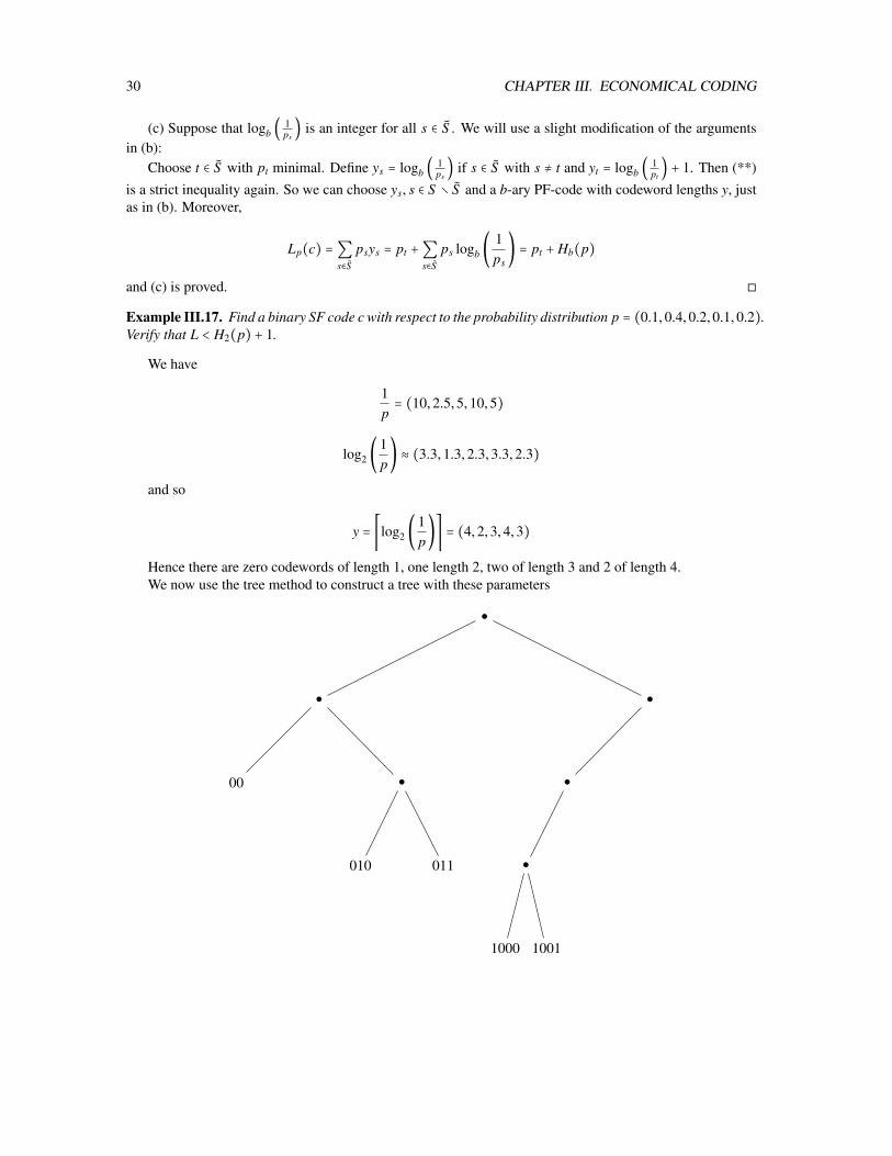
Example III.17. Find a binary SF code c with respect to the probability distribution p = (0.1,0.4,0.2,0.1,0.2).Verify that L < H2(p) + 1.
We have
1p= (10,2.5,5,10,5)
log2 (1p) ≈ (3.3,1.3,2.3,3.3,2.3)
and so
y = ⌈log2 (1p)⌉ = (4,2,3,4,3)
Hence there are zero codewords of length 1, one length 2, two of length 3 and 2 of length 4.We now use the tree method to construct a tree with these parameters
00
010 011
1000 1001
III.5. HUFMAN RULES 31
Since y = (4,2,3,4,3) we can choose the code c as follows
(1000,00,010,1001,011)
We have
H2(p) = p⋅log2 (1p) ≈ (0.1,0.4,0.2,0.1,0.2)⋅(3.3,1.3,2.3,3.3,2.3) = 0.33+0.52+0.46+0.33+0.46 = 2.08 ≈ 2.1
and
L = p ⋅ y = (0.1,0.4,0.2,0.1,0.2) ⋅ (4,2,3,4,3) = 0.4 + 0.8 + 0.6 + 0.4 + 0.6 = 2.8
Since 2.8 < 2.1 + 1 , the inequality L < H2(p) does indeed hold.
Theorem III.18 (Fundamental Theorem). Let p be a probability distribution on the set S and c an optimalb-ary PF code for S with respect to p. Let L be the average codeword length of c. Then
Hb(p) ≤ L ≤ Hb(p) + 1
Moreover, the second inequality is strict unless ∣S ∣ > 1 and there exists s ∈ S with ps = 1.
Proof. By III.14, Hb(p) ≤ L.By III.16 there exists a b-ary PF code d with Lp(d) ≤ Hp(d) + 1, where the inequality is strict, unless
∣S ∣ > 1 and there exists s ∈ S with ps = 1. Since c is optimal we have L ≤ Lp(d) and so the Theorem isproved.
III.5 Hufman rulesLemma III.19. Let p be a positive probability distribution on the set S and c on optimal b-ary PF-code forS with respect to p. Suppose ∣S ∣ ≥ 2.
(a) Let y be the codeword length of c. If d, e ∈ S with yd < ye, then pd ≥ pe.
(b) Among the codewords of maximal length there exist two which have the same parent.
Proof. (a): Suppose that pd < pe. Then
(peye + pdyd) − (peyd + pdye) = (pe − pd)(ye − yd) < 0
Hence peye+ pdyd > peyd + pdye and so interchanging the codewords for d and e gives a code with smalleraverage length, a contradiction.
(b): Let M be the maximal length of a codeword.Suppose that M = 1. Then any codeword has length 1 and so has the empty message ∅ as its parent. So
any two codewords are codewords of maximal length and have the same parent. Since ∣S ∣ ≥ 2 we see that that(b) b holds in this case.
Suppose next tat M > 1 and by way of contradiction, assume that no two codewords of length M havethe same parent. Let x be a codeword of maximal length, let y be the parent of x and let z be any codeword.Suppose that y is a prefix of z. If z = y,then z would be a prefix x and x ≠ z, a contradiction. Thus z ≠ y andsince y has length M − 1, we conclude that z has length at least M. Since M is the maximal codeword length
32 CHAPTER III. ECONOMICAL CODING
this means that z has length M and y is the parent of z. Since no two codewords of maximal length have thesame parent, this means z = x.
We proved that x is the only codeword with y as a prefix. Hence, replacing each codewords of maximallength by its parent, gives a PF code of smaller average codeword length than c. Since c is an optimal code,this is a contradiction. So (b) is proved.
Theorem III.20. Let p a positive probability distribution on the alphabet S with ∣S ∣ ≥ 2. Let d, e be distinctsymbols in S such that pd ≤ pe ≤ ps for all s ∈ S with s ≠ d. Let S = S ∖ d and let c ∶ S → B
∗ be a binaryPF-code.
Define a probability distribution p on S by
(H1) ps =⎧⎪⎪⎨⎪⎪⎩
ps if s ≠ epd + pe if s = e
Also define the code c ∶ S → T∗ by
(H2) c(s) =
⎧⎪⎪⎪⎪⎨⎪⎪⎪⎪⎩
c(e)0 if s = dc(e)1 if s = ec(s) otherwise
Then
(a) c is a binary prefix free code for S .
(b) L(c) = L(c) + pe, where L(x) is the codeword length of a code x.
(c) c is an optimal binary PF code for S with respect to p if and only if c is a optimal binary PF code for Swith respect to p.
Proof. (a) Since c is prefix free it is readily verified that also c is prefix free.
(b) Put S = S ∖ d, e. Then S = S ∪ e and S = S ∪ d, e. Let y and y be the codeword length for cand c, respectively. Then
ys = ys and ps = ps for all s ∈ S
and
pe = pd + pe, yd = ye + 1, ye = ye + 1
HenceL(c) = ∑s∈S psys
= pdyd + peye +∑s∈S peye
= pd(ye + 1) + pe(ye + 1) +∑s∈S psys
= (pd + pe) + (pd + pe)ye +∑s∈S psys
= pe + peye +∑s∈S psys
= pe +∑s∈S psys
= pe + L(c)

III.5. HUFMAN RULES 33
So (b) holds.
(c)Ô⇒: Suppose c is an optimal binary PFcode. Let a be an optimal binary PF code for p and let a bethe code constructed from a using rule H2 with a in place of c.
Since c is an optimal, L(c) ≤ L(a). Hence also L(c) − pe ≤ L(a) − pe. Applying (b) twice (once to cand once to a) gives L(c) ≤ L(a). Since a is optimal, L(a) ≤ L(c). Thus L(a) = L(c). Since a is optimal, itfollows that c is optimal.
(c) ⇐Ô: Suppose c is an optimal binary PF code. Let a be a optimal binary PF code for p. Let M bethe maximal length of a codeword of a.
Suppose that there exists f ∈ d, e with such that a( f ) as length less than M. By III.19(b) there existsat least two codewords of length M and so we can choose g ∈ S such that a(g) has length l. Then a(l) haslarger length than a(g) and III.19(a) shows that pg ≤ p f . By choices of e and d, p f ≤ pg and so p f = pg. Thusinterchanging the codewords for f and g does not change the average length of a. We therefore may assumethat both a(d) and a(e) have maximal length.
By III.19(b) there exists two codewords of a of maximal length with a common parent. Permuting code-words of equal length does not change the average codeword length. So we may and do choose a such thata(d) and a(e) have a common parent u and that a(d) = u0 and a(e) = u1. Let a be the code for S defined by
a(s) =⎧⎪⎪⎨⎪⎪⎩
u if s = ea(s) if s ∈ S
Since a is PF, u is not a codeword of a. Hence any codeword of a with u as a prefix must have length Mand since a is binary code must be u0 or u1. Hence u is not the prefix of any a(s), s ∈ S . It follows that a isPF-code for S .
Note that a is the code constructed from a via Rule H2. Since a is optimal, the already proven forwarddirection of (c) shows that a is optimal. Since c is optimal this gives L(a) = L(c). Thus also L(a) + pe =L(c)+ pe. From (b) applied to a and c we conclude that L(a) = L(c). Since a is optimal, this means that alsoc is optimal.
Example III.21. Use Hufman’s Rules H1 and H2 to construct an optimal code with respect to the probabilitydistribution (0.3,0.2,0.2,0.15,0.1,0.05)

34 CHAPTER III. ECONOMICAL CODING
0.3
10
0.2
00
0.2
01
0.15
110
0.1
1110
0.05
1111
0.3
10
0.2
00
0.2
01
0.15
110
0.15
111
0.3
10
0.2
00
0.2
01
0.3
11
0.3
10
0.4
0
0.3
11
0.4
0
0.6
1
1
∅

Chapter IV
Data Compression
IV.1 The Comparison TheoremTheorem IV.1 (The comparison theorem). Let p and q probability distributions on the alphabet S and let ba real number larger than 1. Then
Hb(p) ≤∑s∈S
ps logb (1qs
)
with equality and only if p = q.(If ps = qs = 0 we interpret ps logb ( 1
qs) as 0. If ps ≠ 0 and qs = 0 we interpret ps logb ( 1
qs) as ∞ and so
also ∑s∈S ps logb ( 1qs) =∞.)
Proof. If qs = 0 for some s ∈ S with ps ≠ 0, the sum on the right sides is ∞. Thus Hb(p) < ∑s∈S ps logb ( 1qs)
and q ≠ p in this case.So we may assume that qs ≠ 0 for all s ∈ S with ps ≠ 0. We also may remove all s from S for which
ps = qs = 0. So qs ≠ 0 for all s ∈ S and we can define ys = logb ( 1qs). Then 1
bys = qs and so
∑s∈S
1bys
=∑s∈S
qs = 1.
Thus by Theorem III.11 ∑s∈S ps logb ( 1ps) ≤ ∑s∈S psys with equality if and only if ys ≠ 0 and ys =
logb ( 1ps) for all s ∈ S . Hence Hb(p) ≤ ∑s∈S ps logb ( 1
qs) with equality if and only if logb ( 1
qs) = logb ( 1
ps) for
all s ∈ S , that is if and only if qs = ps, for all s ∈ S
Theorem IV.2. Let p be a probability distribution on the alphabet S with m symbols. Let b > 1. Then
Hb(p) ≤ logb m
with equality if and only if p is the equal probability distribution.
Proof. Let q = ( 1m)
s∈Sbe the equal probability distribution on S . Then
∑s∈S
ps logb (1qs
) =∑s∈S
ps logb (11m
) =∑s∈S
ps logb m = (∑s∈S
ps) logb m = logb m
35

36 CHAPTER IV. DATA COMPRESSION
and so by the comparison theorem
Hb(p) ≤ logb m
with equality if and only if p = q.
IV.2 Coding in pairsLemma IV.3. Let I be an alphabet and p an I-tuple with coefficients in R. Then p is a probabilty distributionif and only if
(i) pi ≥ 0 for all i ∈ I.
(ii) ∑i∈I pi = 1.
Proof. If p is a probabilty distribution, then p is a function from I to [0,1] with ∑i∈I pi = 1. So (i) and (ii)holds.
Suppose now that (i) and (ii) holds. Then p j ≥ 0 for all j ∈ I and so
pi ≤ pi +∑j∈Ij≠i
p j =∑j∈I
p j = 1.
Thus 0 ≤ pi ≤ 1 and so pi ∈ [0,1]. Hence p has coefficients in [0,1] and by (ii) p is a probabilitydistribution.
Corollary IV.4. Let I be an alphabet and p an I-tuple with coefficients in R. Suppose that pi ≥ 0 for all i ∈ Iand t = ∑i∈I pi ≠ 0. Then ( pi
t )i∈I is a probability distribution on I.
Proof. Since pi ≥ 0 for all i ∈ I also t ≥ 0 and pit ≥ 0. Also
∑i∈I
pi
t= ∑i∈I pi
t= t
t= 1
and so by IV.3, ( pit )i∈I is a probability distribution on I.
Definition IV.5. Let I and J be alphabets and f an I × J-matrix with coefficients in R. Define the I-tuple f ′
byf ′i =∑
j∈Jfi j
for all i ∈ I and the J-tuple f ′′ byf ′′j =∑
i∈Ifi j
for all j ∈ J. Then f ′ is called the (first) marginal tuple of f an I. f ′′ is called the (second) marginal tuple off on J.
Note that f ′ = ∑ j∈J Col j( f ) is the sum of the columns of f , while f ′′ = ∑i∈I Rowi( f ) is the sum of therows of f .
Lemma IV.6. Let I and J be alphabets and p be a I × J-matrix with coefficients in R+ and marginal tuplesp′ and p′′. Then p is a probablity distribution if and only if p′ is a probability distribution and if and only ifp′′ is a probality distribution.

IV.2. CODING IN PAIRS 37
Proof. Since pi j ≥ 0 we also have p′i ≥ 0 and p′′j ≥ 0 for all i ∈ I, j ∈ J. Also
∑i∈I
p′i =∑i∈I
⎛⎝∑j∈J
pi j⎞⎠= ∑
(i, j)∈I×Jpi j =∑
j∈J(∑
i∈Ipi j) =∑
j∈Jp′′j .
If one p, p′ and p′′ is a probability distributions, then this sum is equal to 1 and so by IV.3 all of p, p′, p′′
are probability distributions.
Definition IV.7. Let I and J be alphabets.
(a) Let f ′ and f ′′ be I and J-tuples, respectively, with coefficients in R. Then f ′ ⊗ f ′′ is the I × J-matrixdefined by
( f ′ ⊗ f ′′)i j = f ′i f ′′j .
for all i ∈ I, j ∈ J.
(b) Let p be a probability distribution on I × J with marginal distribution p′ and p′′. Then p′ and p′′ arecalled independent with respect to p if
p = p′ ⊗ p′′
Lemma IV.8. Let p′ and p′′ be probability distributions on I and J, respectively.
(a) p′ and p′′ are the marginal tuples of p′ ⊗ p′′.
(b) p′ ⊗ p′′ is a probability distribution on I × J.
(c) p′ and p′′ are independent with respect to p′ ⊗ p′′.
Proof. (a) We have
∑j∈J
(p′ ⊗ p′′)i j =∑j∈J
p′i p′′j = p′i⎛⎝∑j∈J
p′′j⎞⎠= p′i ⋅ 1 = p′i
and so p′ is the marginal tuple of p′ ⊗ p′′ on I. Similarly, p′′ is the marginal tuple of p′ ⊗ p′′ on I.(b) By (a) the marginal tuples of p′ ⊗ p′′ are probability distributions and so by IV.6 also p′ ⊗ p′′ is a
probability distribution.(c) Follows immediately from the definition of independent.
Theorem IV.9. Let I and J be alphabets and p be a probability distribution on I × J with marginal distribu-tions p′ and p′′. Then
H(p) ≤ H(p′) + H(p′′)
with equality if and only if p′ and p′′ are independent with respect to p.
Proof. We have

38 CHAPTER IV. DATA COMPRESSION
H(p′) + H(p′′) = ∑i∈I
p′i log( 1p′i
) +∑j∈J
p′′j log( 1p′′j
)
= ∑i∈I
⎛⎝∑j∈J
pi j⎞⎠
log( 1p′i
) +∑j∈J
(∑i∈I
pi j) log( 1p′′j
)
= ∑i∈I, j∈J
pi j (log( 1p′i
) + log( 1p′′j
))
= ∑i∈I, j∈J
pi j log( 1p′i p′′j
)
= ∑s∈I×J
ps log( 1(p′ ⊗ p′′)s
)
Thus the comparison theorem shows that H(p) ≤ H(p′) + H(p′′) with equality if and only if p = p′ ⊗ p′′,that is if and only if p′ and p′′ are independent with respect to p′ and p′′.
IV.3 Coding in blocksDefinition IV.10. A source is a pair (S ,P) where S is an alphabet and P is a function
P ∶ S ∗ → [0,1]
such that
(i) P(∅) = 1, and
(ii) for all a ∈ S ∗,
P(a) =∑s∈S
P(as)
We interpret a source as a device which emits an infinite stream ξ1ξ2 . . . , ξn, . . . of symbols from S .P(a1a2 . . .an) is the probability that ξ1 = a1, ξ2 = a2, . . . , ξn−1 = an−1 and ξn = an.
Definition IV.11. Let (S ,P) be a source and let r ∈ N.
(a) pr is the restriction of P to S r, so pr is the function from S r to the interval [0,1] with pr(a) = P(a) forall a ∈ S r.
(b) p = p1, so p is the restriction of P to S .
(c) Pr is the restriction of P to (S r)∗. Note here that if x = x1x2 . . . xn is a string of length n in the alphabetS r, then each xi is a string of length rin the alphabet S , and so x is a string of length nr in the alphabetS , so (S r)∗ = ⋃∞n=0 S nr ⊆ S ∗.
(d) Let l = (l1, l2, . . . lr) be an increasing r-tuple of positive integers, that is li ∈ Z+ and l1 < l2 < . . . < lr. Putu = lr. For y = y1y2 . . . yu ∈ S u define
yl ∶= yl1 yl2 . . . ylr
and note that yl ∈ S r. Define the function pl from S r to R via

IV.3. CODING IN BLOCKS 39
pl(x) = ∑y∈S u
yl=x
P(y)
for all x ∈ S r.
We interpret pl(s1s2 . . . sr) as the probabilty that ξl1 = s1, ξl2 = s2, . . . , ξlr = sr.Note also that
p(l1,...,lr)(x1x2 . . . xr) = ∑(y1y2...yu)∈S u
yl1=x1,yl2=x2,...,ylr=xr
P(y1y2 . . . yu)
Lemma IV.12. Let (S ,P) be a source, r ∈ N and l = (l1, . . . , lr) be an increasing r-tuple of positive integers.
(a) Let a ∈ S ∗. Then
P(a) = ∑x∈S r
P(ax).
(b) ∑x∈S r P(x) = 1 and pr is a probability distribution on S r.
(c) p is a probability distribution on S .
(d) Put t = lr − r (and so lr = r + t) and let k = (k1, . . . , kt) be the increasing t-tuple of positive integers with1, . . . , t + r = l1, . . . , ll, k1, . . . , kt. Then we can identify S t+r with S t × S r via the map
S t+r → S t × S r,d → (dk,dl)
and, after this identification, pl is the marginal tuple of pt+r on S r.
(e) pl is a probability distribution on S r.
Proof. (a) We will prove (a) by induction on r. If r = 0, then the empty message ∅ is the only element of S r.Hence
∑x∈S r
P(ax) = P(a∅) = P(a)
and (a) holds in this case. Now suppose that (a) holds for r. Since every x ∈ S r+1 can be uniquely written asx = ys with y ∈ S r and s ∈ S we get
∑x∈S r+1
P(ax) = ∑y∈S r ,s∈S
P(a(ys)) = ∑y∈S r
(∑s∈S
P((ay)s)) = ∑y∈S r
P(ay) = P(a)
where the third equality holds by the definition of the source and the last by the induction assumption.(b) Using a = ∅ in (a) we get 1 = P(∅) = ∑x∈S r P(∅x) = ∑x∈S r P(x). Hence by IV.3 is probability
distribution on S r.(c) This is the special case r = 1 in (b).(d) Let a = a1 . . .at ∈ S t and b = b1 . . .br ∈ S r. Define d ∈ S t+r by di = a j if i = k j for some 1 ≤ j ≤ t and
di = b j if i = l j for some 1 ≤ j ≤ r. Then dk = a and dl = b. So the map
ρ ∶ S t × S r → S t+r, (a,b)→ d

40 CHAPTER IV. DATA COMPRESSION
is inverse to the map
S t+r → (S t,S r),d → (dk,dl)
Let y ∈ S t+r and x ∈ S r. Then y = ρ(a,b) for some a ∈ S t and b ∈ S a. Then yl = x if and only if b = x andso if and only if y = ρ(a, x) for unique a ∈ S t. Thus
pl(x) = ∑y∈S t+r
yl=x
P(y) = ∑a∈S t
pt+r(ρ(a, x))
So pl is the marginal tuple of pt+r on S r.(c) By (b), pr+t is a probability distribution on S r+t and by (d), pl is a marginal tuple of pt+r. So by IV.6
pl is a probability distribution on S r.
Lemma IV.13. Let (S ,P) be a source and r ∈ N. Then (S r,Pr) is a source.
Proof. Let a ∈ (S r)∗. Then by IV.12(a)
Pr(a) = P(a) = ∑b∈S r
P(ab) = ∑b∈S r
Pr(ab).
Moreover, Pr(∅) = P(∅) = 1 and so Pr is a source on S r.
IV.4 Memoryless SourcesDefinition IV.14. A source (S ,P) is called memoryless if
P(as) = P(a)P(s)
for all a ∈ S ∗ and s ∈ S .
Lemma IV.15. Let p be a probability distribution on the alphabet S . Define
P ∶ S ∗ → [0,1]
inductively by
P(∅) = 1
andP(as) = P(a)ps
for all a ∈ S ∗, s ∈ S . SoP(s1 . . . sn) = ps1 ps2 . . . psn
Then (S ,P) is the unique memoryless source with P(s) = ps for all s ∈ S .
Proof. Since 0 ≤ ps ≤ 1 for all s ∈ S , also 0 ≤ P(a) ≤ 1 for all a ∈ S ∗. So P is indeed a function from S ∗ to[0,1]. By definition of P, P(∅) = 1. Let a ∈ S ∗. Then
∑s∈S
P(as) =∑s∈S
P(a)ps = P(a)∑s∈S
ps = P(a)1 = P(a)
so P is source.

IV.5. CODING A STATIONARY SOURCE 41
Now let Q be any memoryless source with Q(s) = ps for all s ∈ S . We need to prove that Q(a) = P(a)for all a ∈ S ∗. The proof is by induction on the length n of a. If n = 0, then a = ∅ and Q(a) = 1 = P(a).Suppose now Q(a) = P(a) holds for all messages a of length n and let b be a message of length n + 1. Thenb = as for some message a of length n and some s ∈ S . Thus
Q(b) = Q(as) = Q(a)Q(s) = P(a)ps = P(b)
Thus Q = P and Q is uniquely determined by p.
Lemma IV.16. Let (S ,P) be a memoryless source and let r, t ∈ N. Then pt+r = pt ⊗ pr and so pt and pr areindependent with respect to pt+r.
Proof. Let a = s1 . . . sr ∈ S t and b = st+1 . . . st+r ∈ S r. Then
pt+r(ab) = pt+r(s1 . . . sr sr+1 . . . sr+t)
= ps1 . . . psr psr+1 . . . pt+r
= (ps1 . . . psr)(psr+1 . . . pt+r)
= pt(s1 . . . sr)pr(sr+1 . . . sr+t)
= pt(a)pr(b)
IV.5 Coding a stationary sourceDefinition IV.17. A source (S ,P) is called stationary if
pr = p(1+t,...,r+t)
for all r, t ∈ N.
Since pr = p(1,...,r) we can rewrite the conditions on a stationary source as follows:
p(1,...,r) = p(r+1,...,t+r)
Inductively, this means that the probability of a string s1 . . . sr to appears at the positions 1,2 . . . , r of thestream ξ1ξ2 . . . , ξn . . . is the same as the probability of the string appear to appear at positions t + 1, . . . t + r.
Lemma IV.18. Let (S ,P) be a source. Let r, t ∈ N.
(a) pt and p(t+1,...,t+r) are the marginal distributions of pt+r on S t and S r.
(b) Suppose P is stationary, then pt and pr are the marginal distributions of pr+t on S t and S r.
Proof. (a) By IV.12(a),pt(a) = P(a) = ∑
b∈S r
P(ab) = ∑b∈S r
pt+r(ab)
Hence pt is the marginal distribution of pt+r on S t. The special case l = (t + 1, r + 2, . . . , t + r) andk = (1, . . . .t) in IV.12(d) shows that p(t+1,...,t+r) is the the marginal distributions of pt+r on S r.
(b) Since P is stationary, pr = p(t+1,...,t+r) and so (a) implies (b).
42 CHAPTER IV. DATA COMPRESSION
Lemma IV.19. A memoryless source is stationary.
Proof. Let (S ,P) be a memoryless source and r, t ∈ N. By IV.16 pt+r = pt × pr and so by IV.8(c) , pr is themarginal distribution of pt+r on pr. By IV.18(a), p(t+1,...,t+r) is also the marginal distribution of pt+r on S r.Thus pr = p(t+1,...,t+r) and P is stationary.
Theorem IV.20. Let (S ,P) be a source and let r, t ∈ Z+ and let b > 1.
(a)Hb(pt+r) ≤ Hb(pt) + Hb(p(t+1,...,t+r))
with equality if and only if pt and p(t+1,...,t+r) are independent with respect to pt+r.
(b) Suppose P is stationary. ThenHb(pt+r) ≤ Hb(pt) + Hb(pr)
with equality if and only if pt and pr are independent with respect to pr+t.
(c) Suppose (S ,P) is stationary, and r divides t. Then
Hb(pt)t
≤ Hb(pr)r
.
(d) Supppose (S ,P) is memoryless. ThenHb(pt)
t= Hb(p).
Proof. By IV.18(b) pr and p(t+1,...,pt+r) are the marginal distributions of pt+r on S t and S r. Thus (a) followsfrom IV.9
(b) Since P is stationary, pr = p(t+1,...,t+r) = pt. So (b) follows from (a).
Before proving (c) and (d) we first show:
(*) Let q ∈ Z+. Then Hb(pqr) ≤ qHb(pr), with equality if (S ,P) is memoryless.
For q = 1, (*) is obviously true. Suppose now that (*) holds for q. Then by (b)
Hb(p(q+1)r) = Hb(pqr+r) ≤ Hb(pqr) + Hb(qr) ≤ qHb(pr) + Hb(pr) = (q + 1)Hb(pr)
with equality if (S ,P) is memoryless. (Note here that by IV.16 pqr and pr are independent with respect topqr+r for memoryless sources.) So (∗) holds for q + 1 and hence by the Principal of induction, for all q ∈ Z.
(c) Since r divides t, t = qr for some q ∈ Z+. Thus using (*)Dividing by qr gives
Hb(pt)t
= Hb(pqr)qr
≤ qHb(pr)qr
= Hb(pr)r
.(d) Suppose (S ,P) is memoryless. By (*) applied with q = t and r = 1.
Hb(pt) = Hb(pt⋅1) = tHb(p1) = Hb(p)
and so Hb(pt)t = Hb(p).

IV.5. CODING A STATIONARY SOURCE 43
Definition IV.21. Let (S ,P) be a source and b > 1. Then the entropy of P to the base b is the real number
Hb(P) ∶= lim infm→∞
Hb(pm)m
Recall here that the limit inferior of a sequence (an)∞n=1 of real numbers is defined as
lim infm→∞
am = limm→∞
(∞infn=m
an)
Lemma IV.22. Let (S ,P) be a stationary source. Then
Hb(pn) =∞infn=1
Hb(pn)n
Proof. Let m ∈ Z+. If 1 ≤ n < m we have Hb(pnm)nm ≤ Hb(pn)
n and so
∞infn=m
Hb(pn)n
=∞infn=1
Hb(pn)n
Lemma IV.23. Let (S ,P) be a memoryless source and b > 1. Then Hb(P) = Hb(p).
Proof. Just recall that by IV.20(c) we have Hb(pr)r = Hb(p) for all r ∈ Z+.
Theorem IV.24 (Coding Theorem for memoryless sources). Let (S ,P) be a memoryless source, b an integerwith b > 1 and ε > 0. Let n be an integer with n > 1
ε. Then there exists a b-ary prefix-free code for S n for
which the average codeword length L with respect to pn satisfies
Ln< Hb(p) + ε
Proof. Note that 1n < ε. Also since P is memoryless, Hb(pn)
n = Hb(p).By the Fundamental Theorem, there exists a prefix-free code b-ary code c for S n with average length L
respect to pn satisfying L ≤ Hb(pn) + 1. Then
Ln≤ Hb(pn) + 1
n= Hb(pn)
n+ 1
n< Hb(p) + ε
Theorem IV.25 (Coding Theorem for Sources). Let (S ,P) be a source, b > 1 an integer and ε > 0. Thenthere exists a positive integer n and a b-ary prefix-free code for S n for which the average codeword length Lwith respect to pn satisfies
Ln< Hb(P) + ε.
Proof. Since Hb(P) = limm→∞ (inf∞n=mHb(pn)
n ) there exists a positive integer r such that
∞infn=m
Hb(pn)n
< Hb(P) + ε
2for all m ≥ r. Thus for all m ≥ r there exists n ≥ m with
44 CHAPTER IV. DATA COMPRESSION
(1) Hb(pn)n
< Hb(P) + ε
2
Choose an integer m such that m ≥ r and m > 2ε. Choose n ≥ m as in (1). Then
(2) 1n≤ 1
m< 1
2ε
= ε
2
By the Fundamental Theorem, there exists a prefix-free code b-ary code c for S n with average length Lrespect to pn satisfying
(3) L ≤ Hb(pn) + 1
Combining (1), (2) and (3) we obtain
Ln≤ Hb(pn) + 1
n= Hb(pn)
n+ 1
n< Hb(P) + ε
2+ ε
2= Hb(P) + ε
IV.6 Arithmetic codesDefinition IV.26. Let S be set. Then an ordering on S is a relation ’<’ on S such that for all a,b, c ∈ S :
(i) Exactly one of a < b,a = b and b < a holds; and
(ii) if a < b and b < c, then a < c.
An ordered alphabet is an alphabet together with an ordering ’<’ on S .
Example IV.27. Suppose S = s1, s2, . . . , sm is an alphabet of size m. Then there exists a unique orderingon S with si < si+1 for all 1 ≤ i < n. Indeed we have si < s j if and only if i < j.
Notation IV.28. In the following, “Let S = s1, . . . , sm be an ordered alphabet” will mean that the orderingis given by si < s j if and only if i < j.
Definition IV.29. Let S be an ordered alphabet and p a positive probability distribution in S . Fix s ∈ S anddefine:
α = α(s) =∑t∈St<s
pt,
where α = 0 if s is the smallest element in S ;
n′ = n′(s) = ⌈log2 (1ps
)⌉ ;
n = n(s) = n′ + 1;
c′ = c′(s) = ⌈2nα⌉;

IV.6. ARITHMETIC CODES 45
c(s) = z1z2 . . . zn ∈ B∗,
where
z1, . . . , zn ∈ B with c′ =n
∑i=1
zi2n−i.
Then c ∶ S → B∗, s→ c(s) is called the arithmetic code for S with respect to p.
Example IV.30. Determine the arithmetic code for the order alphabet S = a,d, e,b, c with respect to theprobability distribution p = (0.1,0.3,0.2,0.15,0.25).
s p α 1p n′ n 2nα c′ ∑n
i=1 zi2n−i c
a 0.1 0 10 4 5 0 0 0 ⋅ 16 + 0 ⋅ 8 + 0 ⋅ 4 + 0 ⋅ 2 + 0 00000
d 0.3 0.1 3.3 . . . 2 3 0.8 1 0 ⋅ 4 + 0 ⋅ 2 + 1 001
e 0.2 0.4 5 3 4 6.4 7 0 ⋅ 8 + 1 ⋅ 4 + 1 ⋅ 2 + 1 0111
b 0.15 0.6 6.3 . . . 3 4 9.6 10 1 ⋅ 8 + 0 ⋅ 4 + 1 ⋅ 2 + 0 1010
c 0.25 0.75 4 2 3 6 6 1 ⋅ 4 + 1 ⋅ 2 + 0 110
In the remainder of the section we will prove that arithmetic codes are prefix-free and find an upper boundfor their average codeword length.
Definition IV.31. Let z = z1z2 . . . zn ∈ Bn. Then the rational number
n
∑i=1
zi
2i
is called the rational number associated to z and is denoted by 0∗z.
Observe that 0∗z ≤ ∑ni=1
12i < ∑∞
i=112i = 1. So 0 ≤ 0∗z < 1.
Lemma IV.32. Let n ∈ Z+ and α a real number such that 0 ≤ α < α + 12n < 1.
(a) There exists a unique z ∈ Bn with 0∗z ∈ [α,α + 12n ).
(b) If c = ⌈2nα⌉ and z = z1 . . . zn, then c = ∑ni=1 zi2n−i.
(c) 0∗zy = 0∗z + 12n 0∗y ∈ [α,α + 1
2n−1 ) for all y ∈ B∗.
Proof. (a) and (b): Let z = z1 . . . zn ∈ Bn and put d = ∑ni=1 zi2n−i. Then d ∈ N and
d2n
=n
∑i=1
zi
2i= 0∗z.
Hence0∗z ∈ [α,α + 1
2n )
⇐⇒ d ∈ [2nα,2nα + 1)
⇐⇒ 2nα ≤ d and d < 2nα + 1
⇐⇒ d = ⌈2nα⌉

46 CHAPTER IV. DATA COMPRESSION
This proves (a) and (b).(c) Let y = y1y2 . . . ym. Then yi is the n + i-coefficient of zy and so
α ≤ 0∗z ≤ 0∗zy = 0∗z +∑mi=1
yi2n+i = 0∗z + 1
2n ∑mi=1
yi2i
= 0∗z + 12n 0∗y < 0∗z + 1
2n
< (α + 12n ) + 1
2n = α + 12n−1 .
Thus (c) holds.
Theorem IV.33. Let c be the arithmetic code for the ordered alphabet S with respect to the positive proba-bility distribution p.
(a) For s ∈ S put Is = [α(s), α(s) + ps). Then (Is)s∈S is a partition of [0,1), that is for each r ∈ [0,1), thereexists a unique s ∈ S with r ∈ Is.
(b) 0∗c(s)y ∈ I(s) for all s ∈ S and y ∈ B∗.
(c) c is a prefix-free code.
Proof. (a) Let S = s1, s2, . . . , sm with s1 < s2 < . . . < sm−1 < sm. Observe that α(si) + psi = α(si+1) for all1 ≤ i < m and α(sm) + psm = ∑s∈S ps = 1. Since psi > 0 we have
0 = α(s1) < α(s2) < . . . < α(sm−1) < 1
and for each r ∈ [0,1) there exists a unique 1 ≤ i ≤ m with α(si) ≤ r < α(si+1) (if i < m) and α(si) ≤ r < 1 (ifi = m). Then s = si is the unique element of S with r ∈ Is.
(b) Note that α + 12n < α + 1
2n′ ≤ α + ps ≤ 1 and so we can apply IV.32. It follows that
0∗c(s)y ∈ [α,α + 12n−1
) = [α,α + 12n′ ) ⊆ [α,α + ps) = Is
for all s ∈ S , y ∈ B∗.(c) Let s, t ∈ S with s ≠ t and let y ∈ B∗. By (b), 0∗c(t) ∈ I(t) and 0∗c(s)y ∈ I(s). Hence by (a)
c(t) ≠ c(s)y and so c(s) is neither equal to c(t) nor to a prefix of c(t). Hence c is a prefix-free code.
Theorem IV.34. Let c be the arithmetic code for the ordered alphabet S with respect to the positive proba-bility distribution p. Then
Lp(c) < H2(p) + 2
Proof. Let s ∈ S . Then c(s) has length
n(s) = n′(s) + 1 = ⌈log2 (1ps
)⌉ + 1 < log2 (1ps
) + 2
So
Lp(c) <∑s∈S
ps (log2 (1ps
) + 2) =∑s∈S
ps (log2 (1ps
)) +∑s∈S
2ps = H2(p) + 2

IV.7. CODING WITH A DYNAMIC DICTIONARY 47
Corollary IV.35 (Coding Theorem for Arithmetic codes). Let (S ,P) be a source with p positive. Let ε > 0.Then there exists an integer n with the following property:
Lpn(c)n
< H2(P) + ε
for every arithmetic code c for S n with respect to pn.Moreover, if P is memoryless, any integer n > 2
εhas this property.
Proof. Follow the proof for Coding Theorem for Sources (IV.25) with the following modifications:After Equation (1): Choose m such that m ≥ r and m > 4
ε. So (2) becomes:
(2∗) n > 4ε
After Equation (2): Let c be an arithmetic code on S n with respect to pn. By IV.34 we get
(3∗) Lpn(c) < H(pn) + 2
The changes in (2) and (3) cancel in the last computation in the proof of the Coding Theorem.A similar change in the proof of the Coding Theorem for Memoryless sources gives the extra statement
on memoryless sources.
IV.7 Coding with a dynamic dictionaryDefinition IV.36. An dictionary D based on the alphabet S is a 1-1 N-tuple D = (d1, . . . ,dN) with coefficientsin S ∗. (Here 1-1 means D is 1-1 as a function from 1, . . . ,N to S ∗, that is di ≠ d j for all 1 ≤ i < j ≤ N).
Let d ∈ S ∗. If d = di for some 1 ≤ i ≤ N, we say that d appears in D and call i the index of d in D.
Example IV.37. Let S = s1, s2, . . . , sm be an ordered alphabet. Then D = (s1, . . . , sm) is a dictionary basedon S .
Algorithm IV.38 (LZW encoding). Let S = s1, s2, . . . , sm be an ordered alphabet and X be a non-emptymessage in S . Define
∗ a positive integer n;
∗ non-empty message Yk, 1 ≤ k ≤ n in S ;
∗ positive integer ck, 1 ≤ k ≤ n;
∗ non-empty messages Xk, 0 ≤ k < n in S ;
∗ symbols zk, 1 ≤ k < n in S ; and
∗ dictionaries Dk, 0 ≤ k < n, based on S
inductively as follows:
For k = 0 defineD0 = (s0, s1 . . . , sm) and X0 = X
Suppose k ≥ 1 and that Dk−1 and Xk−1 have been defined.

48 CHAPTER IV. DATA COMPRESSION
Yk is the longest prefix of Xk−1 such that Yk appears in Dk−1. 1
ck is the index of Yk in Dk−1.
If Yk = Xk−1, put n = k and terminate the algorithm. If Yk ≠ Xk−1:
Xk is the (non-empty) message in S with Xk−1 = YkXk.
zk is the first symbol of Xk.
Dk = (Dk−1,Ykzk).2
Put c(X) = c1c2 . . . cn. Also define c(∅) = ∅. The function
c ∶ S ∗ → N∗,X → c(X)
is called the LZW-encoding function for S
Example IV.39. Given the ordered set a,b, c,d, e. Determine the LZW encoding of bdddaad.
b d d d a a d2 4 7 1 1 4
m + k 1 2 3 4 5 6 7 8 9 10
dm+k a b c d e bd dd dda aa ad
So the encoding is 247114.
Lemma IV.40. With the notation as in the LZW encoding algorithm:
(a) Xk = Yk+1Yk+2 . . .Yn for all 0 ≤ k < n.
(b) X = Y1 . . .Yn.
(c) Dk has length m + k and Dk is a prefix of Dl for all 0 ≤ k ≤ l < n.
(d) Yk is the element of index ck in Dl for all k − 1 ≤ l < n.
(e) ykzk is the element appearing with index m + k in Dk for all 1 ≤ k < n.
(f) zk is the first symbol of Yk+1 for all 1 ≤ k < n.
Proof. (a) By construction Xn−1 = Yn. So (a) holds for k = n − 1. By construction Xk−1 = YkXk and (a) holdsby downwards induction.
(b) Since X = X0, this is the case k = 0 in (a).(c) By construction, D0 has length m and Dk−1 is the parent of Dk. So (c) holds by induction.(d) By construction, this holds for l = k − 1. Since Dk−1 is a prefix of Dl for all k − 1 ≤ l < n, (c) follows.(e) By construction, ykzk is the last element of Dk. Since Dk has length m + k, (d) holds.(f) By construction, zk is the first symbol of Xk. So by (a), zk is the first symbol of Yk+1.
Algorithm IV.41 (LZW decoding). Let S = s1, s2, . . . , sm be an ordered alphabet and let u = c1 . . . cn be amessage in N. If u ≠ ∅ and ck < m + k for all 1 ≤ k ≤ n define
1Note that all symbols of S appear in Dk−1 so such a prefix exists and has length at least 12Note that by maximality of Yk , Ykzk does not appear in Dk . So Dk is a dictionary

IV.7. CODING WITH A DYNAMIC DICTIONARY 49
∗ a message Yk, 1 ≤ k ≤ n in S ;
∗ symbols zk, 1 ≤ k < n in S ; and
∗ m + k-tuples Dk, 0 ≤ k < n, with coefficients in S
inductively as follows:
For k = 0 defineD0 = (s1 . . . , sm)
Suppose k ≥ 1 and that Dk−1 already has been defined.
Yk is the the message with index ck appearing in Dk−1.
If k = n, the algorithm stops. If k < n:
If ck+1 < m + k, let Yk+1 be the message with index ck+1 in Dk−1 and let zk be the first symbol of Yk+1.
If ck+1 = m + k, let zk be the first symbol of Yk.3
Dk = (Dk−1,Ykzk).
Put e(u) = Y1 . . .Yn.If u = ∅ or ck ≥ m + k for some 1 ≤ k ≤ n, define e(u) = ∅The function e ∶ N∗ → S ∗,u→ e(u) is called the LZW-decoding for S .
Example IV.42. Find the LZW decoding of the message 4.7.4.3.9.11 for the ordered alphabet b,a, e, f ,d, c.
u 4 7 4 3 9 11
Yk f ff f e fe fef
zk f f e f f fef
dm+k b a e f d c ff fff fe ef fef
m + k 1 2 3 4 5 6 7 8 9 10 11
So the decoding is ffffefefef.
3In this case Yk+1 = Ykzk

50 CHAPTER IV. DATA COMPRESSION
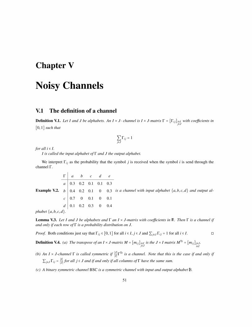
Chapter V
Noisy Channels
V.1 The definition of a channelDefinition V.1. Let I and J be alphabets. An I × J- channel is I × J-matrix Γ = [Γi j] i∈I
j∈Jwith coefficients in
[0,1] such that
∑j∈J
Γi j = 1
for all i ∈ I.I is called the input alphabet of Γ and J the output alphabet.
We interpret Γi j as the probability that the symbol j is received when the symbol i is send through thechannel Γ.
Example V.2.
Γ a b c d e
a 0.3 0.2 0.1 0.1 0.3
b 0.4 0.2 0.1 0 0.3
c 0.7 0 0.1 0 0.1
d 0.1 0.2 0.3 0 0.4
is a channel with input alphabet a,b, c,d and output al-
phabet a,b, c,d.
Lemma V.3. Let I and J be alphabets and Γ an I × J-matrix with coefficients in R. Then Γ is a channel ifand only if each row of Γ is a probability distribution on J.
Proof. Both conditions just say that Γi j ∈ [0,1] for all i ∈ I, j ∈ J and ∑ j∈J Γi j = 1 for all i ∈ I.
Definition V.4. (a) The transpose of an I × J-matrix M = [mi j] i∈Ij∈J
is the J × I matrix MTr = [mi j] j∈Ji∈I
.
(b) An I × J-channel Γ is called symmetric if ∣J∣∣I∣ Γ
Tr is a channel. Note that this is the case if and only if
∑ j∈J Γi j = ∣I∣∣J∣ for all j ∈ J and if and only if all columns of Γ have the same sum.
(c) A binary symmetric channel BSC is a symmetric channel with input and output alphabet B.
51

52 CHAPTER V. NOISY CHANNELS
(d) Let Γ be a binary symmetric channel. Then e = Γ01 is called the bit error of Γ.
Lemma V.5. Let e be the bit error of a binary symmetric channel Γ. Then
Γ =0 1
0 1 − e e1 e 1 − e
Proof. By definition Γ01 = e. Since Γ00 + Γ01 = 1, Γ00 = 1 − e. Since Γ is symmetric the sum of each columnmust be ∣B∣
∣B∣ = 1. So Γ10 = 1 − Γ00 = e and Γ11 = 1 − Γ01 = 1 − e.
Notation V.6. We will usually write an I × J-matrix just as an ∣I∣ × ∣J∣-matrix, that is we do not bother tolist the header row and column. Of course this simplified notation should only be used if a fixed ordering ofelements in I and J is given.
For example we will denote the BSC with error bit e by
BSC(e) =⎡⎢⎢⎢⎢⎢⎣
1 − e e
e 1 − e
⎤⎥⎥⎥⎥⎥⎦
Example V.7. Consider the simplified keypad
A B C
D E F
Two keys are called adjacent if an edge of the one is next to an edge of the other.Suppose that for any two adjacent keys x and y there is a 10% chance that y will be pressed when intending
to press x.
The channel is
Γ A B C D E F
A 0.8 0.1 0 0.1 0 0
B 0.1 0.7 0.1 0 0.1 0
C 0 0.1 0.8 0 0 0.1
D 0 0 0 0.8 0.1 0
E 0 0.1 0 0.1 0.7 0.1
F 0 0 0.1 0 0.1 0.8
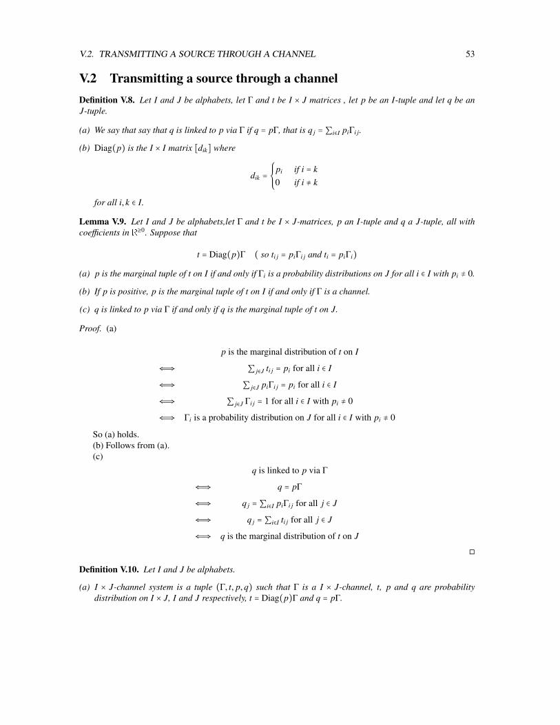
V.2. TRANSMITTING A SOURCE THROUGH A CHANNEL 53
V.2 Transmitting a source through a channelDefinition V.8. Let I and J be alphabets, let Γ and t be I × J matrices , let p be an I-tuple and let q be anJ-tuple.
(a) We say that say that q is linked to p via Γ if q = pΓ, that is q j = ∑i∈I piΓi j.
(b) Diag(p) is the I × I matrix [dik] where
dik =⎧⎪⎪⎨⎪⎪⎩
pi if i = k0 if i ≠ k
for all i, k ∈ I.
Lemma V.9. Let I and J be alphabets,let Γ and t be I × J-matrices, p an I-tuple and q a J-tuple, all withcoefficients in R≥0. Suppose that
t = Diag(p)Γ ( so ti j = piΓi j and ti = piΓi)
(a) p is the marginal tuple of t on I if and only if Γi is a probability distributions on J for all i ∈ I with pi ≠ 0.
(b) If p is positive, p is the marginal tuple of t on I if and only if Γ is a channel.
(c) q is linked to p via Γ if and only if q is the marginal tuple of t on J.
Proof. (a)
p is the marginal distribution of t on I
⇐⇒ ∑ j∈J ti j = pi for all i ∈ I
⇐⇒ ∑ j∈J piΓi j = pi for all i ∈ I
⇐⇒ ∑ j∈J Γi j = 1 for all i ∈ I with pi ≠ 0
⇐⇒ Γi is a probability distribution on J for all i ∈ I with pi ≠ 0
So (a) holds.(b) Follows from (a).(c)
q is linked to p via Γ
⇐⇒ q = pΓ
⇐⇒ q j = ∑i∈I piΓi j for all j ∈ J
⇐⇒ q j = ∑i∈I ti j for all j ∈ J
⇐⇒ q is the marginal distribution of t on J
Definition V.10. Let I and J be alphabets.
(a) I × J-channel system is a tuple (Γ, t, p,q) such that Γ is a I × J-channel, t, p and q are probabilitydistribution on I × J, I and J respectively, t = Diag(p)Γ and q = pΓ.

54 CHAPTER V. NOISY CHANNELS
(b) Let Γ be a I × J-channel and p a probability distribution on T . Then t = Diag(p)Γ is called the jointdistribution for Γ and p. (Γ, t, p, pΓ) is called the Channel system for Γ and p and is denoted by Σ(Γ, p).
(c) Let t be a probability distribution on I × J with marginal distribution p and q and Γ an I × J-channel, Γ iscalled a channel associated to t (and (Γ, t, p,q) is called a channel system associated to t) if t = Diag(p)Γ.
(d) Let Σ = (Γ, t, p,q) be an I × J channel system. Let i ∈ I and j ∈ J. Then
• ti j is called the probability that i is send and j is received and is denoted by PrΣ(i, j).
• pi is called probability that i is send, and is denoted by PrΣ(i,∗).
• q j is called the probability that j is received, and is denoted by PrΣ(∗, j).
• Γi j is called the probability that j is received when i is send and is denoted by PrΣ( j∣i).
Assuming that there is no doubt underlying channel system, we will usually drop the superscript Σ.
Example V.11. Compute the channel system for the channel BSC(e) and the probability distribution (p,1−p).
t = Diag (p,1 − p))BSC(e)
=
⎡⎢⎢⎢⎢⎢⎢⎢⎣
p 0
0 1 − p
⎤⎥⎥⎥⎥⎥⎥⎥⎦
⎡⎢⎢⎢⎢⎢⎢⎢⎣
1 − e e
e 1 − e
⎤⎥⎥⎥⎥⎥⎥⎥⎦
=
⎡⎢⎢⎢⎢⎢⎢⎢⎣
p(1 − e) pe
(1 − p)e (1 − p)(1 − e)
⎤⎥⎥⎥⎥⎥⎥⎥⎦
=
⎡⎢⎢⎢⎢⎢⎢⎢⎣
p − pe pe
e − pe 1 − p − e + pe
⎤⎥⎥⎥⎥⎥⎥⎥⎦Since q is the column sum of t:
q = (p(1 − e) + (1 − p)e, pe + (1 − p)(1 − e)) = (p + e − 2pe,1 + 2pe − p − e)
As a more concrete example consider the case e = 0.1 and p = 0.3. Then
Γ =⎡⎢⎢⎢⎢⎢⎣
0.9 0.1
0.1 0.9
⎤⎥⎥⎥⎥⎥⎦,
t =⎡⎢⎢⎢⎢⎢⎣
0.3 0
0 0.7
⎤⎥⎥⎥⎥⎥⎦
⎡⎢⎢⎢⎢⎢⎣
0.9 0.1
0.1 0.9
⎤⎥⎥⎥⎥⎥⎦=⎡⎢⎢⎢⎢⎢⎣
0.27 0.03
0.07 0.63
⎤⎥⎥⎥⎥⎥⎦and since q is the column sum of t
q = (0.34,0.66)

V.3. CONDITIONAL ENTROPY 55
Lemma V.12. Let I and J be alphabets and Let t be a probability distribution, p the marginal distribution oft on I and Γ an I × J-matrix.
(a) Γ is a channel associated to t if and only if
(i) Γi = 1pi
ti for all i ∈ I with pi ≠ 0, and
(ii) Γi is a probability distribution on J for all i ∈ I with pi = 0
(b) There exists a channel associated to t.
(c) If p is positive, then Diag(p)−1Γ is the unique channel associated to associated to t.
Proof. (a) Suppose first that Γ is a channel associated to t. Then t = Diag(p)Γ and so ti = piΓi. Thus (a:i)holds. Since Γ is channel, also (a:ii) holds.
Suppose next that (a:i) and (a:ii) holds. If pi = 0, then since pi = ∑ j∈J ti j and ti j = 0, also ti j = 0 forall j ∈ J. Thus ti = piΓi for all i ∈ I. Hence t = Diag(p)Γ. From V.9 we conclude that Γi is a probabilitydistribution on J for all i ∈ I with pi ≠ 0. Together with (a:ii) this shows that Γ is a channel.
(b) Let Γ be the I × J-matrix such that Γi = 1pi
ti if pi ≠ 0 and Γi is the equal probability distribution on J ifpi = 0. Then by (a) Γ is a channel associated to t.
(c) Follows immediately from (a).
V.3 Conditional EntropyDefinition V.13. Let Σ = (Γ, t, p,q) be a channel system.
(a) H(t) is called the joint entropy of p and q and is denoted by HΣ(p,q).
(b) H(t) − H(q) is called the conditional entropy of p given q with respect to t, and is denoted by HΣ(p∣q)and H(Γ; p).
(c) H(t) − H(p) is called the conditional entropy of q given p with respect to t, and is denoted by HΣ(q∣p).
(d) H(p) + H(q) − H(t) is called the mutual information of p and q with respect to t and is denoted byIΣ(p,q).
Definition V.14. (a) Let f be an I tuple and g a J-tuple. We say that f is a permutation of g if there exists abijection π ∶ J → I with g j = fπ( j) for all j ∈ J.
(b) Let Γ be a I × J-channel and E a probability distribution on J. We say that Γ is additive with rowdistribution E if each row of Γ is a permutation of E.
Example V.15. (0,1,0,3,0.4,0,2) is a permutation of (0.4,0.2,0.3,0.1).
Example V.16. BSC(e) is additive with row distribution E = (e,1 − e).
Lemma V.17. (a) Let p and p′ be probability distributions. If p is a permutation of p′, then H(p) = H(p′).
(b) Let (Γ, t, p,q) be a channel system. Suppose that Γ is additive with row distribution E. Then t is apermutation of p⊗ E and
H(t) = H(p) + H(E) H(p∣q) = H(p) + H(E) − H(q)
H(q∣p) = H(E) I(p,q) = H(q) − H(E)

56 CHAPTER V. NOISY CHANNELS
Proof. (a) H(p) and H(p′) are sums of the same numbers pi log ( 1pi), just in a different order.
(b) The i’th row of t is piΓi and the i’th row of p⊗ E is piE. Since Γi is a permutation of E, also piΓi is apermutation of piE. So t is a permutation of p⊗ E. Thus by (a) and IV.9
H(t) = H(p⊗ E) = H(p) + H(E)
HenceH(p∣q) = H(t) − h(q) = H(p) + H(E) − H(q),
H(q∣p) = H(t) − h(p) = H(E)
and
I(p,q) = H(p) + H(q) − H(t) = H(q) − H(E)
Corollary V.18. Let (BSC(e), t, p,q) be a channel system. Then
H(p∣q) = H(p) + H((e,1 − e)) − H(q)
V.4 Capacity of a channelTheorem V.19. Let (Γ, t, p,q) be a channel system. Then
I(p,q) ≥ 0
with equality of if p and q are independent with respect to t.
Proof. Note that I(p,q) ≥ 0 if and only if H(t) ≤ H(p) + H(q). Since p and q are the marginal distributionof t, the result now follows from IV.9
Of course one does not want the output of the channel to be independent of the input. So one likes I(p,q)to be as large as possible. This leads to the following definition:
Definition V.20. Let Γ be a I × J channel and let P(I) be set probability distribution on I. Define
fΓ ∶ P(I)→ R, p→ IΣ(Γ,p)(p, pΓ)
and
γ(Γ) = max fΓ = maxp∈P(I)
fΓ(p)
Then γ(Γ) is called the capacity of the channel Γ.
In little less precise notation
γ(Γ) = maxp
I(p,q)
V.4. CAPACITY OF A CHANNEL 57
Theorem V.21. Let Γ be an additive I × J channel with row distribution E. Then
γ(Γ) = ( maxp∈P(I)
H(pΓ)) − H(E) ≤ log ∣J∣ − H(E)
with equality if and only if pΓ is the equal probability distribution on J for some probability distribution p onI.
Proof. Let p ∈ P(I) and (Γ, t, p,q) the channel system for Γ and p. So q = pΓ and t = Diag(p)Γ. By V.17
I(p,q) = H(q) − H(E)
Since γ(Γ) = maxp I(p,q) the first equality holds. By IV.2 H(q) ≤ log ∣J∣ with equality if and only if q isthe equal probability distribution. Hence also the second inequality holds.
Corollary V.22. Let Γ be an symmetric, additive I × J channel with row distribution E. Then
γ(Γ) = log ∣J∣ − H(E)
Proof. Let p = ( 1∣I∣)i∈I be the equal probability distribution on I. Let j ∈ J. We compute
q j =∑i∈I
piΓi j =1∣I∣∑i∈I
Γi j =1∣I∣
∣I∣∣J∣
= 1∣J∣
where the second equality holds since Γ is symmetric. So q is the equal probability distribution on J. SinceΓ is additive, the Corollary now follows from V.21
Corollary V.23. γ(BSC(e)) = 1 − H((e,1 − e)) = 1 − e log ( 1e ) − (1 − e) log ( 1
1−e).
Proof. Since BSC(e) is a symmetric, additive channel with row distribution (e,1− e) and output alphabet ofsize 2, this follows immediately from V.22.
Lemma V.24. Let (Γ, t, p,q) be a channel system. Then
H(q∣p) =∑i∈I
pi H(Γi) = ∑(i, j)∈I×J
ti j log( 1Γi j
)
Proof. Recall that p is the marginal distribution for t on I and so
(1) pi =∑j∈J
ti j
Also
(2) pi
ti j= pi
piΓi j= 1
Γi j.

58 CHAPTER V. NOISY CHANNELS
We compute
H(q∣p) = H(t) − H(p)
= ∑(i, j)∈I×J
ti j log( 1ti j
) −∑i∈I
pi log( 1pi
)
(1)= ∑(i, j)∈I×J
ti j log( 1ti j
) −∑i∈I
⎛⎝∑j∈J
ti j⎞⎠
log( 1pi
)
= ∑(i, j)∈I×J
ti j log( pi
ti j)
(2)= ∑(i, j)∈I×J
ti j log( 1Γi j
)
= ∑(i, j)∈I×J
piΓi j log( 1Γi j
)
= ∑i∈I
pi⎛⎝∑j∈J
Γi j log( 1Γi j
)⎞⎠
= ∑i∈I
pi H(Γi)

Chapter VI
The noisy coding theorems
VI.1 The probability of a mistakeDefinition VI.1. Let I and J be alphabets.
(a) An I × J-decision rule is a function σ ∶ J → I.
(b) Let i ∈ I and j in J. Then (i, j) is called a mistake for σ if i ≠ σ( j).
(c) An I × J-decision system is a tuple (Γ, t, p,q, σ), where (Γ, t, p,q) is a I × J-channel system and σ anI × J- decision rule.
(d) Let Γ be a I × J-channel, p a probability distribution of I and σ and I × J decision rule. Let (Γ, t, p,q)be the channel system for Γ and p. Then (Γ, t, p,q, σ) is called the decision system for Γ, p and σ and isdenoted by Σ(Γ, p, σ).
Definition VI.2. Let Σ = (Γ, t, p,q, σ) be an I × J-decision system. Let i ∈ I.
(a) Then Fσ(i) = j ∈ J ∣ σ( j) ≠ i.
(b) MΣ(i) = ∑ j∈Fσ(i) Γi j. MΣ(i) is called the probability of a mistake if i is send.
(c) MΣ = ∑i∈I pi MΣ(i). MΣ is called the probability of a mistake.
Of course we will often drop the superscripts.
Definition VI.3 (Ideal Observer Rule). Let Σ = (Γ, t, p,q, σ) be an I × J-decision system. We say that σ is anIdeal observer rule with respect to Σ if for all i ∈ I and j ∈ J,
ti j ≤ tσ( j) j
Since Pr(i∣ j) = ti j
q j, this is equivalent to
Pr(i∣ j) ≤ Pr(σ( j)∣ j) for all j ∈ J with q j ≠ 0
Example VI.4. Find the Ideal Observer Rule for the channel BSC(0.3) and probability distribution (0.2,0.8).What is the probability of a mistake?
59

60 CHAPTER VI. THE NOISY CODING THEOREMS
We have
Γ =⎡⎢⎢⎢⎢⎢⎣
0.7 0.3
0.3 0.7
⎤⎥⎥⎥⎥⎥⎦and t =
⎡⎢⎢⎢⎢⎢⎣
0.2 0
0 0.8
⎤⎥⎥⎥⎥⎥⎦
⎡⎢⎢⎢⎢⎢⎣
0.7 0.3
0.3 0.7
⎤⎥⎥⎥⎥⎥⎦=⎡⎢⎢⎢⎢⎢⎣
0.14 0.06
0.24 0.56
⎤⎥⎥⎥⎥⎥⎦Let σ be an ideal observer rule. The largest entry in the first column of t occurs in the second row. So
σ(0) = 1. The largest entry in the second column of t occurs in the second row. So σ(1) = 1. So the receiveralways decides that 1 was send, regardless on what was received.
The mistakes are (0,0) and (0,1). Thus
F(0) = 0,1 and F(1) = So
M(0) = Γ00 + Γ01 = 1 and M(1) = 0
Hence
M = p0M(0) + p1M(1) = 0.2 ⋅ 1 + 0.8 ⋅ 0 = 0.2
Definition VI.5 (Maximum Likelihood Rule ). Let Σ = (Γ, t, p,q, σ) be a I × J-decision system. We say thatσ is a Maximum Likelihood Rule with respect to Γ if for all i ∈ I and j ∈ J
Γi j ≤ Γσ( j) j
Since Γi j = Pr( j∣i), this is the same as
Pr( j∣i) ≤ Pr( j∣σ( j))for all i ∈ I and j ∈ J.
Example VI.6. Find the Maximum Likelihood rule for channel BSC(0.3). What is the probability of amistake with respect to the probability distribution (0.2,0.8)?
We have
Γ =⎡⎢⎢⎢⎢⎢⎣
0.7 0.3
0.3 0.7
⎤⎥⎥⎥⎥⎥⎦Let σ be a Maxumim Likelihood rule. The largest entry in the first column of Γ occurs in the first row, So
σ(0) = 0. The largest entry in the second column of t occurs in the second row. So σ(1) = 1. So the receiveralways decides that the symbol received was the symbol send.
The mistakes are (0,1) and (1,0). Thus
F(0) = 1 and F(1) = 0So
M(0) = Γ01 = 0.3 and M(1) = Γ10 = 0.3
Hence
M = p0M(0) + p1M(1) = 0.2 ⋅ 0.3 + 0.8 ⋅ 0.3 = 0.3
VI.2. FANO’S INEQUALITY 61
VI.2 Fano’s inequalityLemma VI.7. Let (Γ, t, p,q, σ) be an I × J-decision system. M the probability of a mistake and K the set ofmistakes. Then
(I × J) ∖ K = (σ( j), j) ∣ j ∈ J,
M = ∑(i, j)∈K
ti j and 1 − M =∑j∈J
tσ( j) j
Proof. Note that K = (i, j) ∈ I × J ∣ σ( j) ≠ i. So
(I × J) ∖ K = (i, j) ∈ I × J ∣ i = σ( j) = (σ( j), j) ∣ j ∈ J
and the first statement is proved.We compute
∑(i, j)∈K ti j = ∑(i, j)∈I×Jσ( j)≠i
ti j = ∑i∈I (∑ j∈F(i) ti j)
= ∑i∈I (∑ j∈F(i) piΓi j) = ∑i∈I pi (∑ j∈F(i) Γi j)
= ∑i∈I piM(i) = M
Thus the second statement holds. Since 1 = ∑(i, j)∈I×J ti j, the first two statement imply the third.
Theorem VI.8 (Fano’s inequality). Let (Γ, t, p,q, σ) be an I × J-decision system and M the probability of amistake. Then
H(Γ; p) ≤ H((M,1 − M)) + M log (∣I∣ − 1)
Proof. Let K be the sets of mistakes. By VI.7 M = ∑(i, j)∈K ti j and 1 − M = ∑ j∈J tσ( j) j. Thus
H((M,1 − M)) = M log ( 1M ) + (1 − M) log ( 1
1−M )
= ∑(i, j)∈K ti j log ( 1M ) + ∑ j∈J tσ( j) j log ( 1
1−M )
Also by VI.7
I × J = K ⊍ (σ( j), j) ∣ j ∈ J.
Let ∆ = [ ti j
q j] j∈J
i∈I. By Exercise 9(f) on Homework 3
H(Γ; p) = H(p ∣ q) =∑j∈J
q jH(∆ j)
=∑j∈J
q j (∑i∈I
∆ ji log( 1∆ ji
)) =∑j∈J∑i∈I
q jti j
q jlog
⎛⎝
1ti j
q j
⎞⎠
= ∑(i, j)∈I×J
ti j log(q j
ti j) = ∑
(i, j)∈Kti j log(
q j
ti j) +∑
j∈Jtσ( j) j log(
q j
tσ( j) j)

62 CHAPTER VI. THE NOISY CODING THEOREMS
Put
S 1 = ∑(i, j)∈K
ti j log(q j
ti j) − ∑
((i, j)∈Kti j log( 1
M) = ∑
(i, j)∈Kti j log(
Mq j
ti j)
and
S 2 =∑j∈J
tσ( j) j log(q j
tσ( j) j) −∑
j∈Jtσ( j) j log( 1
1 − M) =∑
j∈Jtσ( j) j log(
(1 − M)q j
tσ( j) j) .
Then
H(Γ; p) − H((M,1 − M)) = S 1 + S 2.
So it suffices to show S 1 ≤ M log(∣I∣ − 1) and S 2 ≤ 0.For (i, j) ∈ K put
vi j =ti j
Mand wi j =
q j
∣I∣ − 1.
Since ∑(i, j)∈K ti j = M, (vi j)(i, j)∈K is a probability distribution on K. Also
∑(i, j)∈K
q j =∑j∈J
∑i∈I
i≠σ( j)
q j =∑j∈J
(∣I∣ − 1)q j = (∣I∣ − 1)∑j∈J
q j = ∣I∣ − 1,
and so also (wi j)(i, j)∈K is a probability distribution on K . Thus by the Comparison Theorem IV.1
0 ≥ ∑(i, j)∈K vi j log ( 1vi j) −∑(i, j)∈K vi j log ( 1
wi j)
= ∑(i, j)∈K vi j log (wi j
vi j)
= ∑(i, j)∈Kti j
M log ( q j Mti j(∣I∣−1))
= ∑(i, j)∈Kti j
M log ( q j Mti j
) −∑(i, j)∈Kti j
M log (∣I∣ − 1))
= 1M S 1 + log(∣I∣ − 1)
Thus indeed S 1 ≤ M log(∣I∣ − 1).For j ∈ J, put
u j =tσ( j) j
1 − M.
Since∑ j∈J tσ( j) j = 1−M both q and (u j) j∈J are probability distributions on J. So by the Comparison TheoremIV.1
0 ≥ ∑ j∈J u j log ( 1u j) −∑ j∈J u j log ( 1
q j)
= ∑ j∈J u j log ( q j
u j)
= ∑ j∈Jtσ( j) j
1−M log ( q j(1−M)tσ( j) j
)
= 11−M S 2
and so indeed S 2 ≤ 0.

VI.3. A LOWER BOUND FOR THE PROBABILITY OF A MISTAKE 63
VI.3 A lower bound for the probability of a mistakeTheorem VI.9. Let (Γ, t, p,q, σ) be an I × J-decision system and M the probability of a mistake. Then
M > H(p) − γ(Γ) − 1log(∣I∣)
In particular, if p is the equal probability distribution, then
M > 1 − γ(Γ) + 1log(∣I∣)
Proof. By the Fano inequality VI.8
(∗) H(Γ; p) ≤ H((M,1 − M)) + M log(∣I∣ − 1) ≤ log 2 + M log(∣I∣ − 1)) < 1 + M log(∣I∣)
By definition of the capacity,
γ(Γ) ≥ I(p,q) = H(p) + H(q) − H(t) = H(p) − H(Γ; p)
and so
H(p) − γ(Γ) ≤ H(Γ; p)
So (*) implies
H(p) − γ(Γ) < 1 + M log(∣I∣)
and thus
M > H(p) − γ(Γ) − 1log ∣I∣
So the first statement holds. If p is the equal probability distribution, then by IV.2 H(p) = log(∣I∣) and so
M > log(∣I∣) − γ(Γ) − 1log ∣I∣
= 1 − γ(Γ) + 1log ∣I∣
VI.4 Extended ChannelsLet Γ be an I × J channel and Γ′ be an I′ × J′ channel. Suppose the two channel are ‘unrelated’. The pair ofchannels is used to send a pair of symbols ii′, namely i is send via Γ and i′ via Γ′. Then the probability thatthe pair of symbols j j′ is received is Γi jΓ
′i′ j′ . So the combined channel Γ′′ has input I × I′, output J × J′ and
Γ′′ii′, j j′ = Γi jΓ′i′ j′ .
This leads to the following definitions:

64 CHAPTER VI. THE NOISY CODING THEOREMS
Definition VI.10. (a) Let M be an I × J-matrix and M′ an I′ × J′ matrix Put I′′ = I × I′ and J′′ = J × J′.Then M′′ = M ⊗ M′ is the I′′ × J′′-matrix defined by
m′′ii′, j j′ = mi jm′
i′ j′
M′′ is called tensor product of M and M′.
(b) M be an I × J-matrix and n a positive integer then M⊗n is the In × Jn matrix inductively defined by
M⊗1 = M and M⊗(n+1) = M⊗n ⊗ M
Example VI.11. Compute
a b c
d 0 1 2
e 3 −1 0
⊗
v w
x 4 5
y −1 3
and
⎡⎢⎢⎢⎢⎢⎣
0.2 0.8
0.3 0.7
⎤⎥⎥⎥⎥⎥⎦
⊗2
av aw bv bw cv cw
dx 0 0 4 5 8 10
dy 0 0 −1 3 −2 6
ex 12 15 −4 −5 0 0
ey −3 9 1 −3 0 0
and
⎡⎢⎢⎢⎢⎢⎢⎢⎢⎢⎢⎢⎣
0.04 0.16 0.16 0.64
0.06 0.14 0.24 0.56
0.06 0.24 0.14 0.56
0.09 0.21 0.21 0.49
⎤⎥⎥⎥⎥⎥⎥⎥⎥⎥⎥⎥⎦
Lemma VI.12. Let Γ be an I×J-channel and Γ′ an I′×J′ channel. Put I′′ = I×I′, J′′ = J×J′ and Γ′′ = Γ⊗Γ′.Then
(a) Γ′′ii′ = Γi ⊗ Γ′i′ for all i ∈ I, i′ ∈ I′.
(b) Γ′′ is an I′′ × J′′-channel.
(c) Let n ∈ Z+. Then Γ⊗n is an In × Jn- channel, called the n-fold extension of Γ.
(d) For all x ∈ In, y ∈ Jn, Γ⊗nxy =∏n
k=1 Γxkyk .
Proof. (a)(Γ′′ii′) j j′ = Γ′′ii′, j j′ = Γi jΓ
′i′ j′ = (Γi) j(Γ′i′) j′ = (Γi ⊗ Γi′) j j′
(b) Let i ∈ I and i′ ∈ I′. Since Γ and Γ′ are channels, Γi is a probability distribution on J and Γ′i′ is aprobability distribution on J′. Thus by IV.8, Γi ⊗ Γ′i′ is a probablity distribution on J′′ = J × J′. So by (a) allrows of Γ′′ are probability distributions and hence Γ′′ is a channel.
(c) Follows from (b) and induction on n.(d) Can be proved using an easy induction argument.
Lemma VI.13. Let Γ be an I × J-channel and Γ′ an I′ × J′-channel. Put Γ′′ = Γ ⊗ Γ′ and suppose Σ′′ =(Γ′′, t′′, p′′,q′′) is a channel system. Let t and t′ be the marginal distribution for t′′ on I × J and I′ × J′,respectively. Let p and p′ be the marginal distribution for p′′ on I and I′, respectively. Let q and q′ be themarginal distribution for q′′ on J and J′, respectively
(a) Σ = (Γ, t, p,q) and Σ′ = (Γ′, t′, p′,q′) are channel system.

VI.4. EXTENDED CHANNELS 65
(b) If p and p′ are independent with respect to p′′, then q and q′ are independent with respect to q′′.
(c) Let i ∈ I and i′ ∈ I′. , then H(Γ′′ii′) = H(Γi) + H(Γ′i′).
(d) H(q′′∣p′′) = H(q∣p) + H(q′∣p′)
(e) γ(Γ′′) = γ(Γ) + γ(Γ′).
Proof. Since Σ′′ is a channel system
(1) t′′ii′, j j′ = p′′ii′Γ′′ii′, j j′ = p′′ii′Γi jΓ
′i′ j′
Since Γ′ is a channel, ∑i∈I Γ′i′ j′ = 1. Also t and p are marginal distributions of t′′ and p′′. So summing (1)over all i′ ∈ I′, j′ ∈ J′ gives
ti j = ∑i′∈I′, j∈J′
t′′ii′, j j′ =⎛⎝∑i′∈I′
⎛⎝
p′′ii′ ∑j′∈J′
Γ′i′ j′⎞⎠⎞⎠
Γi j = (∑i′∈I′
p′′ii′)Γi j = piΓi j
So t is the joint distribution of p and Γ.Since Σ′′ is a channel system, q′′ is the marginal distribution of t′′ on J′′ = J × J′. Also q is the marginal
distribution of q′′ on J. It follows that q is the marginal distribution of t′′ on J. Also t is the marginaldistribution of t′′ on I × J. Hence the marginal distribution of t on J is the marginal distribution of t′′ on Jand so equal to q. Thus Σ is a channel system. By symmetry also Σ′ is a channel system.
(b) Suppose that p and p′ are independent with respect to p′′. Then p′′ii′ = pi p′i′ and
q j j′ = ∑i∈I,i′∈I′
p′′ii′Γ′′ii′, j j′ = ∑
i∈I,i′∈I′pi p′i′Γ
′i jΓ
′′j j′ = (∑
i∈IpiΓi j)(∑
i′∈I′p′i′Γ
′i′ j′) = q jq′j′
Hence q′′ = q⊗ q′ and q and q′ are independent with respect to q′′.(c) Let i ∈ I and i′ ∈ I′. By VI.12(a),
Γii′ = Γi ⊗ Γ′i′
and so (c) follows from IV.9.(d) By V.24
H(q′′∣p′′) = ∑i∈I,i′∈I′
p′′ii′H(Γii′)
and so by (c)
H(q′′∣p′′) =∑i∈I
(∑i′∈I′
p′′ii′) H(Γi) +∑i′∈I′
(∑i∈I
p′′ii′) H(Γ′i′) =∑i∈I
piH(Γi) +∑i′∈I′
p′i′H(Γ′i′)
Two more applications of V.24 give (d).(e) Let P be the set of probability distributions on I × I′. Recall that
γ(Γ′′) = maxp′′∈P
fΓ′′(p′′)
and
66 CHAPTER VI. THE NOISY CODING THEOREMS
(2) fΓ′′(p′′) = I(p′′,q′′) = H(p′′) + H(q′′) − H(t′′) = H(q′′) − H(q′′∣p′′).
Since q and q′ are the marginal distributions of q′′ IV.9 gives
(3) H(q′′) ≤ H(q) + H(q′)
with equality if q and q′ are independent with respect to q′′, and so by (b) with equality if p and p′ areindependent with respect to p′′.
Thus
(4)
fΓ′′(p′′) (2)= H(q′′) − (H(q′′∣p′′))(3)≤ H(q) + H(q′) − (H(t′′) − H(q′′))(c)= H(q) + H(q′) − (H(q∣p)) + (H(q′∣p′))
= ((H(q) − (H(q∣p))) + ((H(q′) − (H(q′∣p′)))(2)= fΓ(p) + fΓ′(p′)
with equality in the independent case. Since fΓ(p) ≤ γ(Γ) and fΓ′(p′) ≤ γ(Γ′) we conclude that
fΓ′′(p′′) ≤ γ(Γ) + γ(Γ′).Since this holds for all p ∈ P ,
(5) γ(Γ′′) = maxp′′∈P
fΓ(p′′) ≤ γ(Γ) + γ(Γ′).
Let pmax be a probability distribution on I with fΓ(pmax) = γ(Γ), and p′max be a probability distributionon I′ with fΓ′(p′max) = γ(Γ′). Put p′′max = pmax ⊗ p′max. Then pmax and p′max are independent with respect top′′max and so by (4)
fΓ′′(p′′max) = fΓ(pmax) + fΓ′(p′max) = γ(Γ) + γ(Γ′).Since γ(Γ′′) ≥ fΓ′′(p′′max), this gives
γ(Γ′′) ≥ γ(Γ) + γ(Γ′.)
Together with (5) this gives (e).
Corollary VI.14. Let n be a positive integer.
(a) Let Γ be a channel. Then γ(Γ⊗n) = nγ(Γ).
(b) γ(BSC⊗n(e)) = n(1 − H((e,1 − e))).
Proof. (a) This clearly holds for n = 1. Suppose its true for n. Then
γ(Γ⊗(n+1)) = γ(Γ⊗n ⊗ Γ) = γ(Γ⊗n) + γ(Γ) = nγ(Γ) + γ(Γ) = (n + 1)γ(Γ)Thus (a) also holds for n + 1 and thus for all n,(b) Since H(BSC(e)) = 1 − H((e,1 − e)), (b) follows from (a).

VI.5. CODING AT A GIVEN RATE 67
VI.5 Coding at a given rateDefinition VI.15. Let I and J be alphabets with ∣J∣ > 1. Then the information rate of I relative to J is log∣J∣ ∣I∣.
Note that log∣J∣ ∣I∣ =log ∣I∣log ∣J∣ and log∣Jn∣ ∣I∣ =
log∣J∣ ∣I∣n .
Theorem VI.16 (Noisy Coding Theorem I). Let ρ > 0 be a real number and let Γ be an I × J channel. Let(ni)∞i=1 be an increasing sequence of integers, (Ci)∞i=1 a sequence of sets Ci ⊆ Ini , and (σi)∞i=1 a sequence ofCi × Jni -decision rules σi
Let Mi be the probability of a mistake for the decision system determined by the channel Γ⊗ni ∣Ci×Jni , theequal probability distribution on Ci and the decision rule σi. Suppose that
(i) log ∣Ci∣ni
≥ ρ for all i ∈ Z+, and
(ii) limi→∞ Mi = 0.
Then ρ ≤ γ(Γ).
Proof. Let Γi be the channel Γ⊗ni ∣Ci×Jni . By VI.9
(1) Mi > 1 − γ(Γi) + 1log(∣Ci∣)
By C.1 in the Appendix, γ(Γi) ≤ γ(Γ⊗ni) and by VI.14 γ(Γni) = niγ(Γ). Thus
(2) γ(Γi) ≤ niγ(Γ).
By (i)
(3) log ∣Ci∣ ≥ ρni.
Substituting (2) and (3) into (1) gives
Mi > 1 − niγ(Γ) + 1niρ
= 1 − γ(Γ)ρ
− 1niρ
.
Thus
γ(Γ)ρ
> 1 + Mi −1
niρ
By (ii) we have limi→∞ Mi = 0. Since (ni)∞i=1 is increasing, limi→∞1
niρ= 0. Hence γ(Γ)
ρ≥ 1 and so
ρ ≤ γ(Γ).
Theorem VI.17 (Noisy Coding Theorem II). Let ρ > 0 and Γ an I × J channel. Suppose that ρ < γ(Γ). Thenthere exists an increasing sequence of positive integers (ni)∞i=1 and a sequence (Ci)∞i=1 of sets Ci ⊆ Ini suchthat
(i) log ∣Ci∣ni
≥ ρ for all i ∈ Z+,
68 CHAPTER VI. THE NOISY CODING THEOREMS
(ii) If (pi)∞i=1 is a sequence of probability distributions pi on Ci, then there exists a sequence (σi)∞i=1 ofCi × Jni decision rules σi such that
limi→∞
Mi = 0
where Mi is probability of a mistake for the decision system determined by the channel Γ⊗ni ∣Ci×Jni , theprobability distribution pi and the decision rule σi.
Proof. Beyond the scope of these lecture notes.
VI.6 Minimum Distance Decision RuleDefinition VI.18. Let x, y ∈ Bn. Then d(x, y) = i ∣ 1 ≤ i ≤ n, xi ≠ yi. d(x, y) is called the Hamming distanceof x and y.
Definition VI.19. Let C ⊆ Bn be a code (so C is the set of codewords of a binary code all of whose codewordshave the same length). Let a ∈ C and z ∈ Bn.
(a) A decision rule for C is decision rule for C × Bn, that is a function σ ∶ Bn → C.
(b) Let σ be a decision rule for C. We say that σ is a Minimum Distance rule if for all a ∈ C and z ∈ B
d(a, z) ≥ d(σ(z), z)
Example VI.20. Let σ be a Minimum Distance rule for the code
0011 1000,1100 0001,0000 1110,1100 1011
What is σ(11001001)?
0011 1000 1100 0001 0000 1110 1100 10111100 1001 1100 1001 1100 1001 1100 1001
5 1 5 1
So σ(1100 1001) is either 1100 0001 or 1100 1011.
Lemma VI.21. Let Γ = BSC(e), n ∈ Z+ and x, y ∈ Bn. Then
Γ⊗nxy = ed(1 − e)n−d
Proof. We have
Γ⊗nxy =
n
∏k=1
Γxkyk
Observe that Γxkyk = e if xk ≠ yk and Γxkyk = 1− e if xk = yk. Note that there are d k’s with xk ≠ yk and n− dk’s with xk = yk. So Γ⊗n
xy = ed(1 − e)n−d
Lemma VI.22. Let 0 < e < 12 , C ⊆ Bn and σ a decision rule for C. Then σ is a minimal distance rule if and
only if σ is a maximum likelihood rule with respect to BSC⊗n(e).

VI.6. MINIMUM DISTANCE DECISION RULE 69
Proof. Let z ∈ Bn, a ∈ Bn and put a′ = σ(z). Let d = d(a, z) and d′ = d(a′, z) and f = 1−ee . Since e < 1
2 ,1 − e > 1
2 > e and so f > 1. We compute
Γa′z
Γaz= ed′(1 − e)n−d′
ed(1 − e)n−d= (1 − e
e)
d−d′
= f d−d′
It follow that
Γaz ≤ Γa′z ⇐⇒ d ≥ d′
So Γa′z is maximal if and only if d′ is minimal.
Example VI.23. Suppose C = 000,111. Determine a minimal distance rule σ for C. Compute F(c), Mc
and M for the decision system determined by BSC(e), (p,1 − p) and σ.
We have
σ(z) =⎧⎪⎪⎨⎪⎪⎩
000 if at least two coordinates are zero111 if at most one coordinate is zero
Hence
F000 = 011,101,110,111 and F111 = 000,001,010,100.
So
M000 = Γ000,011 + Γ000,101 + Γ000,110 + Γ000,111
= e2(1 − e) + e2(1 − e) + e2(1 − e) + e3
= e2(3(1 − e) + e)= e2(3 − 2e)
By symmetry, also M111 = e2(3 − 2e) and so
M = pe2(3 − 2e) + (1 − p)e2(3 − 2e) = e2(3 − 2e).
Note that each of the four summand in M000 is at most e2. So M000 ≤ 4e2 and also M ≤ 4e2.

70 CHAPTER VI. THE NOISY CODING THEOREMS

Chapter VII
Error Correcting
Definition VII.1. Let C ⊆ Bn be a code and σ a decision rule for C. Let a ∈ C and z ∈ Bn.
(a) Let k ∈ N. (a, z) is called a k-bit error if d(a, z) = k.
(b) We say that σ corrects (a, z) if a = σ(z).
(c) We say that σ is r-error correcting if σ corrects all k-bit errors for 0 ≤ k ≤ r.
Example VII.2. Given the code C = 000,110,101,011 (so C consist of all even messages of length 3) andthe decision rule
σ ∶000 100 010 001 110 101 011 111
000 011 000 101 110 101 011 110
Does σ correct 0-bit errors? Does σ correct 1-bit errors?
0-bit errors are of the form (a,a),a ∈ C. Since σ(a) = a for all a ∈ C, all 0-bit error are corrected. So σis 0-error correcting.
σ corrects some 1-bit errors but not all:
σ(001) = 101 ≠ 011
Thus (101,001) is a 1-bit error corrected by σ, but (011,001) is a 1-bit error not corrected by σ. So σ isnot 1-error correcting.
Example VII.3. Given the code C = 000 000,110 110,101 101,011 011. (Note that C is obtained bydoubling the code in VII.2). Define the decision rule σ for C by
σ(xy) =⎧⎪⎪⎨⎪⎪⎩
xx if x is evenyy if x is odd
for all x, y ∈ B3. Show that σ is 1-error correcting.
Let (a, z) be k-bit error for k ≤ 1. Since a ∈ C, a = bb for some even b inB3. Let z = xy with x, y ∈ B3. Sincebb and xy differ in at most 1 place, b = x or b = y. Suppose b = x. Since b is even we get σ(xy) = xx = bb = a.If b ≠ x, b must differ in exactly one place from x. So x is odd and σ(xy) = yy = bb = a. So σ is indeed1-error correcting.
71

72 CHAPTER VII. ERROR CORRECTING
Lemma VII.4. Let C ⊆ Bn. Let Σ be a decision system with channel BSC⊗n(e) and an r-error-correctingdecision rule.
(a) d(a, z) ≥ r + 1 for any mistake (a, z).
(b) Γaz ≤ er+1 for any a ∈ C, z ∈ F(a).
(c) Ma ≤ ∣F(a)∣er+1 for any a ∈ C.
(d) M ≤ (∑a∈C pa∣F(a)∣) er+1.
Proof. (a) Let a ∈ C and z ∈ Bn with d(a, z) ≤ r. Since σ is r-correcting, σ(z) = a and so (a, z) is not amistake.
(b) Since z ∈ F(a), (a, z) is a mistake. Put d = d(a, z), then by (a) d ≥ r + 1. Hence
Γaz = ed(1 − e)n−d = er+1ed−(r+1)(1 − e)n−d ≤ er+1
(c) Ma = ∑z∈F(a) Γaz ≤ ∑z∈F(a) er+1 = ∣F(a)∣er+1.
(d) M = ∑a∈C paMa ≤ ∑a∈C pa∣F(a)∣er+1 = (∑a∈C pa∣F(a)∣)er+1.
VII.1 Minimum DistanceDefinition VII.5. Let C ⊆ Bn be a binary code.
(a) δ = δ(C) = mind(a,b) ∣ a,b ∈ C,a ≠ b. δ is called the minimum distance of C.
(b) For a,b ∈ Bn define D(a,b) = i ∣ ai ≠ bi,1 ≤ i ≤ n.
Example VII.6. Compute the minimum distance of the code
000 000,111 000,001 110,110 011
The distances of 000 000 to the other codewords are 3, 3 and 4. Also
111 000 111 000 001 110001 110 110 011 110 011
4 3 5
So the minimum distance is 3.
Definition VII.7. Let A and B be sets. Then
A + B = (A ∪ B) ∖ (A ∩ B)
A + B is called the symmetric difference of A and B.
Lemma VII.8. Let A and B be sets.
(a) A + B = (A ∖ B) ⊍ (B ∖ A).
(b) ∣A + B∣ = ∣A ∖ B∣ + ∣A ∖ B∣ = ∣A∣ + ∣B∣ − 2∣A ∩ B∣.
Proof. Readily verified.

VII.1. MINIMUM DISTANCE 73
Lemma VII.9. Let a,b, c ∈ Bn.
(a) D(a, c) = D(a,b) + D(b, c).
(b) d(a, c) = d(a,b) + d(a, c) − 2∣D(a,b) ∩ D(b, c)∣.
(c) d(a, c) ≤ d(a,b) + d(b, c), with equality if and only if D(a,b) ∩ D(b, c) = ∅.
Proof. (a) Let 1 ≤ i ≤ n.If i ∉ D(a,b) ∪ D(b, c), then ai = bi = ci and so i ∉ D(a, c).If i ∈ D(a,b) ∖ D(b, c), then ai ≠ bi = ci and so ai ≠ ci and i ∈ D(a, c).If i ∈ D(b, c) ∖ D(a,b), then ai = bi ≠ ci and so ai ≠ ci and i ∈ D(a, c).If i ∈ D(a,b) ∩ D(b, c), then ai ≠ bi ≠ ci. Since B only has two elements this gives ai = ci and so
i ∉ D(a, c).Hence i ∈ D(a, c) if and only of i ∈ (D(a,b) ∖ D(b, c)) ∪ (D(b, c) ∖ D(a,b))) = D(a,b) + D(b, c)(b) and (b):
d(a, c) = ∣D(a, c)∣ = ∣D(a,b) + D(b, c)∣ = ∣D(a,b)∣ + ∣D(b, c)∣ − 2∣D(a,b) ∩ D(b, c)∣
= d(a,b) + d(b, c) − 2∣D(a,b) ∩ D(b, c)∣ ≤ d(a,b) + d(b, c)
with equality if and only if ∣D(a,b) ∩ D(b, c)∣ = 0, that is if D(a,b) ∩ D(b, c) = ∅.
Lemma VII.10. Let a,b ∈ Bn. Put d = d(a,b) and let 0 ≤ e ≤ d. Then there exists x ∈ Bn with d(a, x) = e andd(x,b) = d − e.
Proof. Let J be a subset of D(a,b) with ∣J∣ = e. Define x ∈ Bn by xi = bi if i ∈ J and xi = ai if i ∉ J. Sinceai ≠ bi for all i ∈ J we have D(a, x) = J and so d(a, x) = ∣J∣ = e. Since D(a, x) = J ⊆ D(a,b) we concludefrom VII.9 that
D(x,b) = D(x,a) + D(a,b) = J + D(a,b) = D(a,b) ∖ J
and
d(x,b) = ∣D(a,b) ∖ J∣ = ∣D(a,b)∣ − ∣J∣ = d − e.
Definition VII.11. Let r,n ∈ N, x ∈ Bn and X ⊆ Bn. Then
Nr(x) = y ∈ Bn ∣ d(x, y) ≤ r
and
Nr(X) = y ∈ Bn ∣ d(x, y) ≤ r for some x ∈ X
Nr(x) is called the neighborhood of radius r around x.
Example VII.12. Compute N1(0110).
N1(0110) = 0110,1110,0010,0100,0111

74 CHAPTER VII. ERROR CORRECTING
Lemma VII.13. Let C ⊆ Bn be a code, σ an decision rule for σ. Then σ is r-error correcting if and only ifσ(z) = a for all a ∈ C and all z ∈ Nr(a).
Proof. σ is r-error correcting if and only if no k-bit error (a, z) with k ≤ r is a mistake. This holds if andonly if σ(z) = a for all a ∈ C and z ∈ Bn with d(a, z) ≤ r and so if and only if σ(z) = a for all a ∈ C andz ∈ Nr(a).
Definition VII.14. A binary code C is called an r-error correcting code if δ ≥ 2r + 1, that is d(a,b) ≥ 2r + 1for all a,b ∈ C with a ≠ b.
Theorem VII.15. Let C ⊆ Bn and r ∈ N. Then the following are equivalent:
(a) C is an r-error correcting code.
(b) For each z ∈ Bn, there exists at most one a ∈ C with d(a, z) ≤ r.
(c) Nr(a) ∩ Nr(b) = ∅ for all a,b ∈ C with a ≠ b.
(d) Any minimum distance decision rule for C is r-error correcting.
(e) There exists an r-error correcting decision rule for C.
Proof. (a)Ô⇒ (b): Suppose C is an r-error correcting code. Then C has minimal distance at least 2r + 1.Let z ∈ Bn and a,b ∈ C with d(a, z) ≤ r and d(b, z) ≤ r. Then d(a,b) ≤ d(a, z) + d(z,b) ≤ r + r = 2r < 2r + 1.Since C is minimal distance at least 2r + 1, a = b. So there exists at most one codeword of distance less orequal to r from z.
(b) Ô⇒ (c): Suppose Nr(a) ∩ Nr(b) ≠ ∅ and let z ∈ Nr(a) ∩ Nr(b). Then d(a, z) ≤ r and d(b, z) ≤ r,contradiction to (b).
(c) Ô⇒ (d): Let σ be minimal distance decision rule and (a, z) be a k-bit error with k ≤ r. Thend(a, z) = k ≤ r. Put b = σ(z). Since σ is a minimal distance decision rule d(b, z) ≤ d(a, z) ≤ r. Thusz ∈ Nr(a) ∩ Nr(b) and (c) implies that a = b. So σ corrects (a, z) and σ is r-error correcting.
(d)Ô⇒ (e): Obvious.
(e)Ô⇒ (a): Let a,b ∈ C with a ≠ b and put d = d(a,b). Let d = 2e + ε where ε ∈ 0,1 and e ∈ N. ByVII.10 there exists z ∈ Bn with d(a, z) = e and d(x,b) = d− e = e+ ε. Since a ≠ b, σ(a) ≠ a or σ(z) ≠ b. So atleast one of (a, z) and (b, z) is a mistake. Hence σ is not (e + ε)-error-correcting and so r < e + ε. It followsthat r ≤ e, d = e + (e + ε) > r + r = 2r and d ≥ 2r + 1. Thus δ(C) ≥ 2r + 1 and C is r-error correcting,
VII.2 The Packing BoundLemma VII.16. Let r,n ∈ N with r ≤ n and x ∈ Bn.
(a) ∣y ∈ Bn ∣ d(x, y) = r∣ = (nr).
(b) ∣Nr(x)∣ = ∑ri=0 (
ni).
Proof. (a) The mapy→ D(x, y)
is bijection between y ∈ Bn ∣ d(x, y) = r and the set of subsets of size r of 1, . . . ,n.(b) Note that Nr(x) is the disjoint union of the sets y ∈ Bn ∣ d(x, y) = i, 0 ≤ i ≤ r. So (a) follows from
(b).

VII.2. THE PACKING BOUND 75
Lemma VII.17. Let C ⊆ Bn and r ∈ N. Then
(a) ∣Nr(C)∣ ≤ 2n with equality if and only if ∣Nr(C)∣ = Bn.
(b) ∣Nr(C)∣ ≤ ∣C∣∑ri=0 (
ni) with equality if and only if C is an r-error correcting code.
Proof. (a) Just observe that Nr(C)) ⊆ Bn and ∣Bn∣ = 2n.(b) Note that Nr(C) = ⋃a∈C Nr(a) and so
(1) ∣⋃a∈C
Nr(a)∣ ≤∑a∈C
∣Nr(a)∣
with equality if and only if Nr(a) ∩ Nr(b) = ∅ for all a,b ∈ C with a ≠ b. So by VII.15 with equality if andonly if C is r-error-correcting.
By VII.16(b)
(2) ∑a∈C
∣Nr(a)∣ =∑a∈C
r
∑i=0
(nk) = ∣C∣
r
∑i=0
(ni)
Combining (1) and (2) gives (b).
Theorem VII.18 (The Packing Bound). Let C ⊆ Bn be an r-error-correcting code. Then
∣C∣ ⋅r
∑i=0
(ni) ≤ 2n
and so
∣C∣ ≤ 2n
∑ro=0 (
ni)
Proof. By VII.17
∣C∣ ⋅r
∑i=0
(ni) = ∣Nr(C)∣ ≤ 2n
Definition VII.19. Let C ⊆ Bn be a code. Then the information rate ρ(C) of C is the information rate of Crelative to ∣Bn. That is
ρ(C) = log∣Bn∣ ∣C∣ = log2 ∣C∣n
Example VII.20. Use packing theorem to find an upper bound for the information rate of a 2-error correctingcode C ⊆ Bn of size 100?
We will first find a lower bound for n.We need 100 (1 + n + (n
2)) ≤ 2n, that is
100(2 + 2n + n2 − n2
) ≤ 2n

76 CHAPTER VII. ERROR CORRECTING
and
25(n2 + n + 2) ≤ 2n−1
Thus also 25n2 ≤ 2n−1 and 5n ≤ 2n−1
2 . Put m = n−12 . Then n = 2m + 1 and so 5(2m + 1) ≤ 2m and
2m − 10m − 5 > 0
Consider the function f (x) = 2x − 10x − 5. Then
f ′(x) = ln(2)2x − 10 > 0 if and only if x > log2 (10ln 2
) ≈ 3.85
Since f (0) = 1 − 0 − 5 < 0 and f (6) = 64 − 60 − 6 < 0, f (x) < 0 on the interval [0,6]. Thus m > 6 andn = 2m + 1 > 13. Hence n ≥ 14 and
ρ(C) ≤ log2 10014
≈ 0.228
Definition VII.21. Let C ⊆ Bn. Then C is called a perfect code if there exists r ∈ N such that for all z ∈ Bn
there exists a unique a ∈ C with d(z,a) = r.
Lemma VII.22. Let C ⊆ Bn. Then C is a perfect code if and only if there exists r ∈ N such that C is an r-errorcorrecting code and
∣C∣r
∑i=0
(ni) = 2n
Proof. By VII.15 C is r-error correcting the following holds for any perfect code and for any r-error correct-ing code:
(*) For each z in Bn, there exists at most one a ∈ C with d(a, z) ≤ r.
Note that this condition holds if C is perfect code. So we may assume that (∗) holds and so C is r-errorcorrecting. Then
C is a perfect code
⇐⇒ for all z ∈ Bn there exists a unique a ∈ C with d(a, z) ≤ r
⇐⇒ for all z ∈ Bn there exists at least one c ∈ C with d(c, z) ≤ r — by (*)
⇐⇒ Bn = Nr(C)
⇐⇒ 2n = ∣Nr(C)∣
⇐⇒ 2n = ∣C∣∑ri=0 (
ni) VII.17(b)
Definition VII.23. Let δ,n ∈ N with δ ≤ n. Then A(n, δ) is the largest possible size of code C ⊆ Bn withminimum distance at least δ. That is
A(n, δ) = maxC⊆Bn
δ(C)≥δ
∣C∣

VII.2. THE PACKING BOUND 77
Note that the code with minimal distance δ will be ⌊ δ−12 ⌋-error correcting. So the packing bound will
provide an upper bound for A(n, δ). But if δ is fairly large this upper bound can be easily improved:
Lemma VII.24. Let δ,n ∈ N with 23 n < δ ≤ n. Then A(n, δ) = 2.
Proof. The code 00 . . .0,11 . . .1 show that A(n, δ) ≥ 2. We will now show that any code C with at leastthree codewords has minimal distance
δ(C) ≤ 23
n.
So suppose a,b, c are three distinct codewords in C and assume without loss d(a,b) ≥ 23 n and d(b, c) ≥ 2
3 n.Then
n ≥ ∣D(a,b) ∪ D(b, c)∣ = ∣D(a,b)∣ + ∣D(b, c)∣ − ∣D(a,b) ∪ D(b, c)∣ ≥ 23
n + 23
n − ∣D(a,b) ∩ D(b, c)∣
and so
∣D(a,b) ∩ D(b, c)∣ ≥ 13
n
Since D(a, c) ∩ (D(a,b) ∩ D(b, c)) = ∅ this gives
∣D(a, c)∣ ≤ n − ∣D(a,b) ∩ D(b, c)∣ ≤ n − 13
n = 23
n
So indeed δ(C) ≤ 23 n.
The packing bound can be much higher: Consider n = 10 and δ = 7. Then r = ⌊ 7−12 ⌋ = 3 and
∣C∣ ≤ 210
1 + (101 ) + (10
2 ) + (103 )
= 10241 + 10 + 45 + 120
= 1024176
< 6
So we only get ∣C∣ ≤ 5 from the packing bound.

78 CHAPTER VII. ERROR CORRECTING

Chapter VIII
Linear Codes
VIII.1 Introduction to linear codesDefinition VIII.1. F2 is the set B = 0,1 together with the following addition and multiplication:
+ 0 1
0 0 1
0 1 0
⋅ 0 1
0 0 0
0 0 1
So for example in F2, 1 + 1 = 0 and 1 ⋅ 0 = 0.
Definition VIII.2. Fn2 is Bn together with the following addition and scalar multiplication
⎛⎜⎜⎜⎜⎜⎜⎜⎜⎝
x1
x2
⋮
xn
⎞⎟⎟⎟⎟⎟⎟⎟⎟⎠
+
⎛⎜⎜⎜⎜⎜⎜⎜⎜⎝
y1
y2
⋮
yn
⎞⎟⎟⎟⎟⎟⎟⎟⎟⎠
=
⎛⎜⎜⎜⎜⎜⎜⎜⎜⎝
x1 + y1
x2 + y2
⋮
xn + yn
⎞⎟⎟⎟⎟⎟⎟⎟⎟⎠
l
⎛⎜⎜⎜⎜⎜⎜⎜⎜⎝
x1
x2
⋮
xn
⎞⎟⎟⎟⎟⎟⎟⎟⎟⎠
=
⎛⎜⎜⎜⎜⎜⎜⎜⎜⎝
kx1
kx2
⋮
kxn
⎞⎟⎟⎟⎟⎟⎟⎟⎟⎠
for all l, x1, . . . , xn, y1, . . . , yn ∈ F2.
If l = 0, then lxi = 0 for all i and so 0x = 0 for all x ∈ Fn2. Here 0 = 00 . . .0. If l = 1, then lxi = xi for all i
and so 1x = x for all x ∈ Fn2.
Recall here that we are viewing
x1x2 . . . xn,
⎛⎜⎜⎜⎜⎜⎜⎜⎜⎝
x1
x2
⋮
xn
⎞⎟⎟⎟⎟⎟⎟⎟⎟⎠
, and (x1, x2, . . . , xn)
as three different notations for the exact same n-tuple with coefficients in B.(The book considers these to be different objects. If x = x1 . . . xn is a message in B then x′ denotes the
corresponding column vector.)
79

80 CHAPTER VIII. LINEAR CODES
Example VIII.3. Compute 11011 + 10110
We have
11011
+ 10110
= 01101
Definition VIII.4. A subspace of Fn2 is a subset C of Fn
2 such that
(a) 0 ∈ C.
(b) lx ∈ C for all l ∈ F2, x ∈ F21.
(c) x + y ∈ C for all x, y ∈ C.
A subspace of Fn2 is also called a binary linear code of length n
Definition VIII.5. Let C be a subspace of Fn2. A basis for C is a k-tuple
(v1, . . . , vk)
in C such that for each c in C there exists a unique k-tuple
(l1, . . . , lk)
in F2 withc = l1v1 + . . . + lkvk.
Lemma VIII.6. Let C be a subspace of Fn2.
(a) C has a basis (v1, . . . , vk).
(b) ∣C∣ = 2k and so k = log ∣C∣.
(c) 0 ≤ k ≤ n.
Proof. (a) See your favorite linear algebra book.(b) By definition of a basis and a subspace the map
Fk2 → C, (l1, . . . , lk)→ l1v1 + . . . + lkvk
is a well-defined bijection. Thus ∣C∣ = ∣Fk2∣ = 2k. (c) Since 1 ≤ ∣C∣ ≤ ∣Fn
2∣ = 2n, this follows from (b).
Example VIII.7. Let C = 000 000,111 000,000 111,111 111. Find a basis for C and determine theparameters of C.
Both(111 000,000 111)
and
(111 000,111 111)are a basis for C and so dimC = 2.
1 Since lx = 0 or lx = x, this condition is redundant

VIII.2. CONSTRUCTION OF LINEAR CODES USING MATRICES 81
Definition VIII.8. Let C be a binary linear code of length n. The length k of a basis of C is called thedimension of C and is denoted by dimC. The triple (n,dimC, δ(C)) are called the parameters of C.
Remark VIII.9. The information rate ρ(C) of a binary linear code C of length n and dimension k is kn .
Proof. Let C ⊆ Fn2 be a linear code. Then
ρ(C) = log2 ∣C∣log2 ∣Fn
2∣= log2 2k
log2 2n= k
n
Definition VIII.10. Let x = x1 . . . xn ∈ Fn2. Then wt(x) = ∣1 ≤ i ≤ n ∣ xi ≠ 0∣ is called the weight of x.
Lemma VIII.11. Let x, y ∈ Fn2.
(a) d(x, y) = wt(x − y) = wt(x + y).
(b) wt(x) = d(x, 0).
(c) Let C be a binary linear code. Then δ(C) is the minimal weight of a non-zero codeword.
Proof. (a)d(x, y) = ∣1 ≤ i ≤ n ∣ xi ≠ yi∣ = ∣1 ≤ i ≤ n ∣ xi − yi ≠ 0 = wt(x − y)
(b) d(x, 0) = wt(x − 0) = wt(x).(c) Let w be the minimal weight of a non-zero codeword.Let x, y ∈ C with x ≠ y. Then x− y ≠ 0 and so d(x, y) = wt(x− y) ≥ w. Since C is subspace of Fn
2, x− y ∈ Cand so δ(C) ≥ w.
Let x be non-zero codeword. Since 0 ∈ C, we have wt(x) = d(0, x) ≥ δ(C). Hence w ≥ δ(C) and soδ(C) = w.
Example VIII.12. Let D = 000 000,111 000,000 111,111 111. Determine the parameters of D.
The length of C is 6. The dimension of C is log2 ∣C∣ =log24 = 2. The weights of the codewords are 0,3,3,6. So the minimum non-zero weight is 3. Thus δ(C) = 3and the parameters are
(6,4,3)
VIII.2 Construction of linear codes using matricesDefinition VIII.13. (a) Let E be an n × k matrix over F2. Then
Col(E) = Ey ∣ y ∈ Fk2.
Col(E) is called the linear code generated by E, and E is called a generating matrix for Col(E).
(b) Let H be a m × n-matrix. Then
Nul(H) = x ∈ Fn2 ∣ Hx = 0
H is called a check matrix for Nul(H).

82 CHAPTER VIII. LINEAR CODES
Lemma VIII.14. (a) Let E be an n × k matrix over F2. Then Col(E) is a subspace of Fn2.
(b) Let H be a m × n-matrix over F2. Then Nul(H) is a subspace of Fn2.
Proof. (a) E0 = 0. So 0 ∈ Col(E). Let a,b ∈ Col(E). Then a = Ex and b = Ey for some x, y ∈ Fk2. Thus
a + b = Ex + Ey = E(x + y)
and so a + b ∈ ColE.(b) H0 = 0 and so 0 ∈ Nul(H). Let a,b ∈ NulH. The Ha = 0 and Hb = 0. Hence
H(a + b) = Ha + Hb = 0 + 0 = 0
and so a + b ∈ NulH.
Example VIII.15. Find the minimal distance of
Col
⎡⎢⎢⎢⎢⎢⎢⎢⎢⎢⎢⎢⎢⎢⎢⎢⎢⎢⎢⎣
1 0 0
0 1 0
0 0 1
1 1 0
0 1 1
1 0 1
⎤⎥⎥⎥⎥⎥⎥⎥⎥⎥⎥⎥⎥⎥⎥⎥⎥⎥⎥⎦
Let x be in the Column space of the matrix. Then
x
⎡⎢⎢⎢⎢⎢⎢⎢⎢⎢⎢⎢⎢⎢⎢⎢⎢⎢⎢⎣
1 0 0
0 1 0
0 0 1
1 1 0
0 1 1
1 0 1
⎤⎥⎥⎥⎥⎥⎥⎥⎥⎥⎥⎥⎥⎥⎥⎥⎥⎥⎥⎦
⎛⎜⎜⎜⎜⎝
a
b
c
⎞⎟⎟⎟⎟⎠
=
⎛⎜⎜⎜⎜⎜⎜⎜⎜⎜⎜⎜⎜⎜⎜⎝
a
b
c
a + b
b + c
a + c
⎞⎟⎟⎟⎟⎟⎟⎟⎟⎟⎟⎟⎟⎟⎟⎠
for some a,b, c ∈ F2.If exactly one of a,b and c are non-zero, one of the first three coefficient is non-zero and two of the last
three coefficient are non-zero. So wt(x) = 3If exactly two of the a,b, c are not zero, two of the first three coefficient are non-zero and two of the last
three coefficient are non-zero, so wt(x) = 4If all of a,b, c are non-zero, the first three coefficient are non-zero and the last three coefficient are zero.
So wt(x) = 3.Thus Col(E) has minimum weight three and so is 1-error correcting.

VIII.3. STANDARD FORM OF CHECK MATRIX 83
VIII.3 Standard form of check matrixNotation VIII.16. Let (Ia)a∈A and (Jb)b∈B be tuples of sets. Let M = [Mab]a∈A
b∈Bbe an A × B matrix such that
each Mab is an Ia × Jb-matrix. Put I = ⊍a∈A Ia and J = ⊍b∈B Jb. Then we will view M as an I × J-matrix with
Mi j = (Mab)i j
for all i ∈ I, j ∈ J, where a is the unique element of A with i ∈ Ia and b is the unique element of B with j ∈ Jb.
Example VIII.17. Given
X11 =⎡⎢⎢⎢⎢⎢⎣
1 2 3
4 5 6
⎤⎥⎥⎥⎥⎥⎦, X12 =
⎡⎢⎢⎢⎢⎢⎣
7
8
⎤⎥⎥⎥⎥⎥⎦
X21 = [9 10 11] , and X22 = [12] .
Then
[X11,X12] =⎡⎢⎢⎢⎢⎢⎣
1 2 3 7
4 5 6 8
⎤⎥⎥⎥⎥⎥⎦,
⎡⎢⎢⎢⎢⎢⎣
X11
X21
⎤⎥⎥⎥⎥⎥⎦=
⎡⎢⎢⎢⎢⎢⎢⎢⎢⎣
1 2 3
4 5 6
9 10 11
⎤⎥⎥⎥⎥⎥⎥⎥⎥⎦
,
and
⎡⎢⎢⎢⎢⎢⎣
X11 X12
X21 X22
⎤⎥⎥⎥⎥⎥⎦=
⎡⎢⎢⎢⎢⎢⎢⎢⎢⎣
1 2 3 7
4 5 6 8
9 10 11 12
⎤⎥⎥⎥⎥⎥⎥⎥⎥⎦
Definition VIII.18. Let A be a set. Then IA denotes the A × A matrix with ab-coefficient equal to
δab =⎧⎪⎪⎨⎪⎪⎩
1 if a = b0 if a ≠ b
IA is called the A × A identity matrix. If n ∈ N, then In = I1,...,n.
Example VIII.19.
I4 =
⎡⎢⎢⎢⎢⎢⎢⎢⎢⎢⎢⎢⎣
1 0 0 0
0 1 0 0
0 0 1 0
0 0 0 1
⎤⎥⎥⎥⎥⎥⎥⎥⎥⎥⎥⎥⎦
and Ix,y =
x y
x 1 0
y 0 1

84 CHAPTER VIII. LINEAR CODES
Lemma VIII.20. Let A be an m × k matrix in F2. Put
E =⎡⎢⎢⎢⎢⎢⎣
Ik
A
⎤⎥⎥⎥⎥⎥⎦and H = [A Im]
Then
(a) Col(E) = Nul(H).
(b) The columns of E form a basis for Col(E).
(c) Col(E) is a code of length m + k and dimension k.
Proof. (a) Let x ∈ Fk+m2 . Then x =
⎛⎜⎝
a
b
⎞⎟⎠
for unique a ∈ Fk2 and b ∈ Fm
2 . We compute:
⎛⎜⎝
a
b
⎞⎟⎠∈ Col
⎛⎜⎝
⎡⎢⎢⎢⎢⎢⎣
Ik
A
⎤⎥⎥⎥⎥⎥⎦
⎞⎟⎠
⇐⇒⎛⎜⎝
a
b
⎞⎟⎠=⎡⎢⎢⎢⎢⎢⎣
Ik
A
⎤⎥⎥⎥⎥⎥⎦y for some y ∈ Fk
2
⇐⇒⎛⎜⎝
a
b
⎞⎟⎠=⎛⎜⎝
y
Ay
⎞⎟⎠
for some y ∈ Fk2
⇐⇒ a = y and b = Ay for some y ∈ Fk2
⇐⇒ b = Aa
⇐⇒ Aa + b = 0
⇐⇒ [A Il]⎛⎜⎝
a
b
⎞⎟⎠= 0
⇐⇒⎛⎜⎝
a
b
⎞⎟⎠∈ Nul([A Il])
So x ∈ ColE if and only if x ∈ NulH.(b)Consider the map
c ∶ Fk2 → F
m+k2 , y→ Ey =
⎛⎜⎝
y
Ay
⎞⎟⎠
Note thatCol(E) = Ey ∣ y ∈ Fk
2 = c(y) ∣ y ∈ Fk2
and so Col(E) = Im c. Looking at the first k bits of Ey we see that c is 1-1. So α is a bijection from Fk2 to
ColE. Let vi = Col(E). Then

VIII.3. STANDARD FORM OF CHECK MATRIX 85
c(y) = Ey = y1v1 + y2v2 + . . . + ykvk
and since c is a bijection, for each a ∈ Col(E) there exists a unique (y1, . . . , yk) ∈ Fk2 with a = y1v1 + . . . +
ykvk. Hence (v1, . . . , vk) is basis for Col(E).(c) By (b) dim ColE = k. Since ColE ⊆ Fm+k
2 , ColE has length m + k.
We may view c has code for Fk2 in the alphabet B2. Since c(y) = Ey = (y,Ay) the first k-bits of c(y)
(namely y) are called the message bits, and the last m bits (namely Ay) are called the check bits.
Definition VIII.21. Let C ⊆ Bn be a linear code.
(a) A check matrix H for C is said to be in standard form if H = [A Im] for some k ×m matrix A.
(b) A generating matrix E for C is said to be in standard form if E =⎡⎢⎢⎢⎢⎢⎣
Ik
A
⎤⎥⎥⎥⎥⎥⎦for some k ×m-matrix A.
Definition VIII.22. Let C,D ⊆ Fn2. We say that D is a permutation of C if the exist a bijection π ∶ 1, . . . ,n→
1, . . . ,n with
D = aπ(1)aπ(2) . . .aπ(n) ∣ a1a2 . . .an ∈ C
Example VIII.23. Show thatD = 000,100,001,101
is a permutation ofC = 000,010,001,011
D is obtained from C via the permutation:
π ∶1 2 3
2 1 3
Notation VIII.24. Let I, J be sets, i, k ∈ I, A an I × J matrix and x and y J-tuples.
(a) RixA denotes the I × J matrix B with RowiB = x and RowlA = RowlA for all l ∈ I with l ≠ i. (So RixA isthe matrix obtained from A by replacing Row i by x.)
(b) Rik xyA = Rix(RkyA). (So Rik xyA is the matrix obtained from A by replacing Row k by y and thenreplacing Row i by x.)
Definition VIII.25. Let I and J be sets and i, k ∈ I with i ≠ k. Then ’Ri ↔ R j’ and ’Ri + Rk → Rk’ are thefunctions with domain the binary I × J-matrix defined as follows:
(a) (Ri ↔ Rk)(A) = RikakaiA. So Ri → Rk interchangings row i and row k of A
(b) (Ri + Rk → Rk)(A) = Rk(ai + ak)A. So (Ri + Rk → Rk) adds row i to row k of A.
An elementary row operation is one of the function Ri ↔ R j and Ri + Rk → Rk.Elementary column operations are defined similarly, using the symbol C in place of R and using columns
rather that rows.
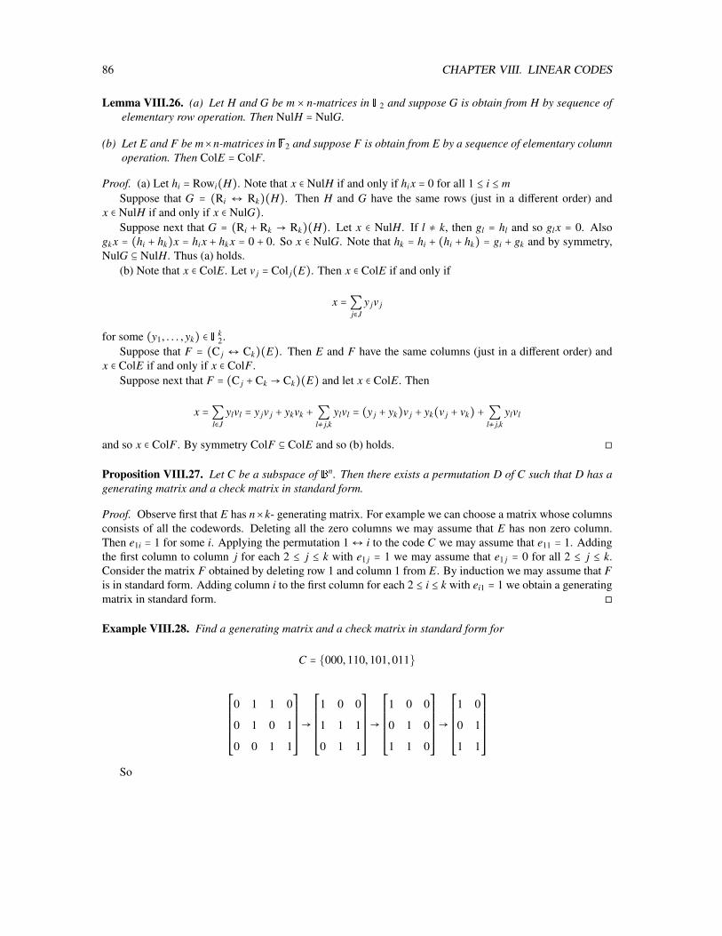
86 CHAPTER VIII. LINEAR CODES
Lemma VIII.26. (a) Let H and G be m × n-matrices in F2 and suppose G is obtain from H by sequence ofelementary row operation. Then NulH = NulG.
(b) Let E and F be m×n-matrices in F2 and suppose F is obtain from E by a sequence of elementary columnoperation. Then ColE = ColF.
Proof. (a) Let hi = Rowi(H). Note that x ∈ NulH if and only if hix = 0 for all 1 ≤ i ≤ mSuppose that G = (Ri ↔ Rk)(H). Then H and G have the same rows (just in a different order) and
x ∈ NulH if and only if x ∈ NulG).Suppose next that G = (Ri + Rk → Rk)(H). Let x ∈ NulH. If l ≠ k, then gl = hl and so glx = 0. Also
gk x = (hi + hk)x = hix + hk x = 0 + 0. So x ∈ NulG. Note that hk = hi + (hi + hk) = gi + gk and by symmetry,NulG ⊆ NulH. Thus (a) holds.
(b) Note that x ∈ ColE. Let v j = Col j(E). Then x ∈ ColE if and only if
x =∑j∈J
y jv j
for some (y1, . . . , yk) ∈ Fk2.
Suppose that F = (C j ↔ Ck)(E). Then E and F have the same columns (just in a different order) andx ∈ ColE if and only if x ∈ ColF.
Suppose next that F = (C j +Ck → Ck)(E) and let x ∈ ColE. Then
x =∑l∈J
ylvl = y jv j + ykvk + ∑l≠ j,k
ylvl = (y j + yk)v j + yk(v j + vk) + ∑l≠ j,k
ylvl
and so x ∈ ColF. By symmetry ColF ⊆ ColE and so (b) holds.
Proposition VIII.27. Let C be a subspace of Bn. Then there exists a permutation D of C such that D has agenerating matrix and a check matrix in standard form.
Proof. Observe first that E has n×k- generating matrix. For example we can choose a matrix whose columnsconsists of all the codewords. Deleting all the zero columns we may assume that E has non zero column.Then e1i = 1 for some i. Applying the permutation 1↔ i to the code C we may assume that e11 = 1. Addingthe first column to column j for each 2 ≤ j ≤ k with e1 j = 1 we may assume that e1 j = 0 for all 2 ≤ j ≤ k.Consider the matrix F obtained by deleting row 1 and column 1 from E. By induction we may assume that Fis in standard form. Adding column i to the first column for each 2 ≤ i ≤ k with ei1 = 1 we obtain a generatingmatrix in standard form.
Example VIII.28. Find a generating matrix and a check matrix in standard form for
C = 000,110,101,011
⎡⎢⎢⎢⎢⎢⎢⎢⎢⎣
0 1 1 0
0 1 0 1
0 0 1 1
⎤⎥⎥⎥⎥⎥⎥⎥⎥⎦
→
⎡⎢⎢⎢⎢⎢⎢⎢⎢⎣
1 0 0
1 1 1
0 1 1
⎤⎥⎥⎥⎥⎥⎥⎥⎥⎦
→
⎡⎢⎢⎢⎢⎢⎢⎢⎢⎣
1 0 0
0 1 0
1 1 0
⎤⎥⎥⎥⎥⎥⎥⎥⎥⎦
→
⎡⎢⎢⎢⎢⎢⎢⎢⎢⎣
1 0
0 1
1 1
⎤⎥⎥⎥⎥⎥⎥⎥⎥⎦
So

VIII.4. CONSTRUCTING 1-ERROR-CORRECTING LINEAR CODES 87
E =
⎡⎢⎢⎢⎢⎢⎢⎢⎢⎣
1 0
0 1
1 1
⎤⎥⎥⎥⎥⎥⎥⎥⎥⎦
and H = [1,1,1]
are a generating matrix and check matrix in standard form for C
VIII.4 Constructing 1-error-correcting linear codesDefinition VIII.29. Let (v1, . . . , vk) be a k-tuple in Fn
2. Then (v1, . . . , vk) is called linearly dependent if thereexists a non-zero (l1, . . . , lk) ∈ Fk
2 with
l1v1 + l2v2 + . . . + lkvk = 0.
(v1, . . . , vk) is called linearly independent, if its is not linearly dependent.
Note that (v1, . . . , vk) is linearly independent if for all (l1, . . . , lk) ∈ Fk2
l1v1 + l2v2 + . . . + lkvk = 0 Ô⇒ l1 = 0, l2 = 0, . . . , lk = 0
Lemma VIII.30. Let H be check matrix for the binary linear code C.
(a) The minimum distance of C is the minimal number of columns of H whose sum is equal to 0. It is alsoequal to the minimal number of linearly dependent columns of H.
(b) Let r ∈ Z+. Then C is r-error-correcting if and only if any sum of 2r or less columns of H is not equal to0.
Proof. Let x = x1x2 . . . xn ∈ Fn with x ≠ 0 and let hi be the i-th column of H. Then
Hx = x1h1 + x2h2 + . . . + xnhn.
Let 1 ≤ i1 < i2 < . . . < id ≤ n such that xi j ≠ 0 for all 1 ≤ j ≤ d and xi = 0 for all other i. Then xi j = 1 and so
Hx = hi1 + hi2 + . . . + hid .
Observe that d = wt(x). Since x ∈ C if only if Hx = 0, we conclude that there exists a vector of weight din C if and only if there exists d columns of H whose sum is equal to 0.
This proves the first statement. Let 1 ≤ k1 < k2 < . . . < ke ≤ n. Then the columns hk1 , . . . ,hke are linearlydependent if and only if there exists a non-zero (l1, l2, . . . , le) ∈ Fe
2 with
(∗) l1hk1 + l2hk2 + . . . lehke = 0.
In a minimal linear dependent set of columns, all the l j will be non-zero (since the columns with l j ≠ 0are still linear dependent). So l j = 1 for all 1 ≤ j ≤ e and (*) becomes
hk1 + hk2 + . . . + hke = 0.
Thus the minimal number of linear dependent columns is also the minimal numbers of columns whosesum is equal to 0.
(b) C is r-error correcting if and only if the minimal distance is at least 2r + 1. By (a) C has minimumdistance less or equal to 2r if and only if there exists 2r or less columns whose sum is zero. So (b) holds.

88 CHAPTER VIII. LINEAR CODES
Corollary VIII.31. Let n, k ∈ Z with k ≤ n and put m = n − k. Let C ⊆ F2 and H be an m × n-matrix in F2.Then the following two statements are equivalent:
(a) C is binary linear 1-error correcting code with check matrix H and dimension k.
(b) C = Nul(H), ColH = Fm2 and the columns of H are non-zero and pairwise distinct.
Proof. By definition H is a check matrix for C if and only if C = NulH. So we may assume C = NulH. Then
dimC = dim NulH = n − dim ColH = k + (m − dim ColH)
Thus dimC = k if and only if dim ColH = m and so if and only if ColH = Fm.We now apply VIII.30 with r = 1. We conclude that C is 1-error correcting if and only the sum of one or
two of the columns is never 0. Since x + y = 0 if and only if x = y, we see that C is 1-error correcting if andonly if the columns of H are non-zero and pairwise distinct.
Lemma VIII.32. (a) Let n, k ∈ Z+. Then there exists a binary linear 1-error correcting code of dimension kand length n if and only if
k ≤ n − ⌈log2(n + 1)⌉
(b) The maximal information rate of an 1-error correcting, binary linear code of length n is
1 − ⌈log2(n + 1)⌉n
Proof. Suppose first that there exist an 1-error-correcting code of length n and dimension n. Then the Packingbound shows
2k(1 + n) ≤ 2n
and so k + log2(1 + n) ≤ n and k ≤ n − log2(1 + n).Suppose next that k ≤ n − log2(1 + n). Put m = n − k. Then m ≤ m + k = n ≤ 2m − 1. Put ei = Coli(Im).
Then ∣Fk2 ∖ 0, e1, . . . , em∣ = 2m − m − 1 ≥ k. So there exists distinct vectors a1, . . . ,ak ∈ Fk
2 ∖ 0, e1, . . . , emLet A be the k ×m matrix with Coli(A) = ai and put H = [A, Im]. Since ColIm = Fm
2 , also ColH = Fm2 . VIII.31
now shows that NulH is a k-dimensional 1-error correcting code of length n.
Note that
limn→∞
1 − ⌈log2(n + 1)⌉n
= 1
So one can construct 1-error-correcting binary linear codes of information rates arbitrarily close to 1.
Definition VIII.33. A Hamming code is a perfect-1-error correcting binary linear code.
Theorem VIII.34. Let C ⊆ Fn2 be a linear code with n ×m check matrix H such that dimC = n −m. Then C
is a Hamming code if and only if n = 2m − 1 and the columns of H are the non-zero vectors of Fm2 (in some
order).
Proof. By VII.22
1. C is a Hamming code if and only if C is 1-error correcting and ∣C∣(1 + n) = 2n

VIII.4. CONSTRUCTING 1-ERROR-CORRECTING LINEAR CODES 89
Since dimC = n −m
∣C∣(1 + n) = 2n ⇐⇒ 2n−m(1 + n) = 2n ⇐⇒ 1 + n = 2m ⇐⇒ n = 2m − 1
By VIII.31 C is 1-error correcting if and only if the columns of H are non-zero and pairwise distinct.Thus
2. C is a Hamming code if and only if and only if the columns of H are non-zero and pairwise distinctand n = 2m − 1.
Since Fm2 has exactly 2m − 1 non-zero vectors (2) implies the theorem.
Corollary VIII.35. Let n ∈ N. Then there exists a Hamming code of length n if and only if n = 2m − 1 forsome m ∈ N, that is if and only if n + 1 is a power of 2. If this is the case, a Hamming code of length n isunique up to permutation.
Proof. The first statement follows directly from Theorem VIII.34. The same Theorem shows that an n ×m-check matrix of an Hamming code of length n is unique up to a permutation of the columns. So also theHamming code is unique up to permutation.
Example VIII.36. Find a Hamming code of length 7.
We have 7 = 23 − 1. So m = 3 and we can choose the check matrix
H =
⎡⎢⎢⎢⎢⎢⎢⎢⎢⎣
1 1 1 0 1 0 0
1 1 0 1 0 1 0
1 0 1 1 0 0 1
⎤⎥⎥⎥⎥⎥⎥⎥⎥⎦So
E =
⎡⎢⎢⎢⎢⎢⎢⎢⎢⎢⎢⎢⎢⎢⎢⎢⎢⎢⎢⎢⎢⎢⎢⎣
1 0 0 0
0 1 0 0
0 0 1 0
0 0 0 1
1 1 1 0
1 1 0 1
1 0 1 1
⎤⎥⎥⎥⎥⎥⎥⎥⎥⎥⎥⎥⎥⎥⎥⎥⎥⎥⎥⎥⎥⎥⎥⎦is a generating matrix. The codewords are
0000000 0001011 1111111 1110100
1000111 1100001 0111000 0011110
0100110 1010010 0111001 0101101
0010101 1001100 1101010 0110011
Lemma VIII.37. Let C be a linear code with check matrix H. Let (c, z) be a 1-bit error for C.
(a) If the error occurred in bit i, then Hz = ColiH.

90 CHAPTER VIII. LINEAR CODES
(b) If C is 1-error-correcting, i is the uniquely determined by ColiH = Hz.
Proof. (a) Let ei = Coli(In). Then z = c + ei and so Hz = H(c + ei) = Hc + Hei = 0 +Coli(H) = Coli(H).
(b) Just recall no two columns of the check matrix of a 1-error correcting binary linear code are thesame.
Example VIII.38. Let C be the binary linear code with check matrix
⎡⎢⎢⎢⎢⎢⎢⎢⎢⎣
1 0 1 1 0 0
1 1 0 0 1 0
0 1 1 0 0 1
⎤⎥⎥⎥⎥⎥⎥⎥⎥⎦(a) Is C 1-error correcting?
(b) Suppose that (a, z) is a 1-bit error with z = 101100. Find z.
(a) The columns of H are non-zero and pairwise distinct. So C is 1-error correcting.
(b)
Hz =
⎡⎢⎢⎢⎢⎢⎢⎢⎢⎣
1 0 1 1 0 0
1 1 0 0 1 0
0 1 1 0 0 1
⎤⎥⎥⎥⎥⎥⎥⎥⎥⎦
⎛⎜⎜⎜⎜⎜⎜⎜⎜⎜⎜⎜⎜⎜⎜⎝
1
0
1
1
1
0
⎞⎟⎟⎟⎟⎟⎟⎟⎟⎟⎟⎟⎟⎟⎟⎠
=
⎛⎜⎜⎜⎜⎝
1
0
1
⎞⎟⎟⎟⎟⎠
So Hz is the third column of H. Hence the error occurred in bit 3 and a = 100110. To confirm
Hz =
⎡⎢⎢⎢⎢⎢⎢⎢⎢⎣
1 0 1 1 0 0
1 1 0 0 1 0
0 1 1 0 0 1
⎤⎥⎥⎥⎥⎥⎥⎥⎥⎦
⎛⎜⎜⎜⎜⎜⎜⎜⎜⎜⎜⎜⎜⎜⎜⎝
1
0
0
1
1
0
⎞⎟⎟⎟⎟⎟⎟⎟⎟⎟⎟⎟⎟⎟⎟⎠
=
⎛⎜⎜⎜⎜⎝
0
0
0
⎞⎟⎟⎟⎟⎠
So 100110 is indeed a codeword.
VIII.5 Decoding linear codesDefinition VIII.39. Let H be a check matrix for the linear code C ⊆ Fn
2 and z ∈ Fn2.
(a) Hz is called the syndrome of z with respect to H.
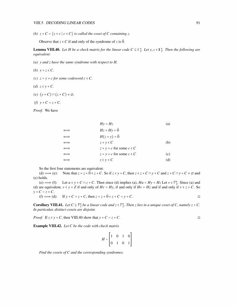
VIII.5. DECODING LINEAR CODES 91
(b) z +C = z + c ∣ c ∈ C is called the coset of C containing z.
Observe that z ∈ C if and only of the syndrome of z is 0.
Lemma VIII.40. Let H be a check matrix for the linear code C ⊆ Fn2. Let y, z ∈ Fn
2. Then the following areequivalent:
(a) y and z have the same syndrome with respect to H.
(b) y + z ∈ C.
(c) z = y + c for some codeword c ∈ C.
(d) z ∈ y +C.
(e) (y +C) ∩ (z +C) ≠ ∅.
(f) y +C = z +C.
Proof. We have
Hy = Hz (a)
⇐⇒ Hz + Hy = 0
⇐⇒ H(z + y) = 0⇐⇒ z + y ∈ C (b)⇐⇒ z + y = c for some c ∈ C
⇐⇒ z = y + c for some c ∈ C (c)⇐⇒ z ∈ y +C (d)
So the first four statements are equivalent.(d)Ô⇒ (e): Note that z = z + 0 ∈ z +C. So if z ∈ y +C, then z ∈ z +C ∩ y +C and z +C ∩ y +C ≠ ∅ and
(e) holds.(e)Ô⇒ (f): Let u ∈ y +C ∩ z +C. Then since (d) implies (a), Hu = Hy = Hz Let v ∈ Fn
2. Since (a) and(d) are equivalent, v ∈ y + Z if and only of Hv = Hy, if and only if Hv = Hz and if and only if v ∈ z +C. Soy +C = z +C.
(f)Ô⇒ (d): If y +C = z +C, then z = z + 0 ∈ z +C = y +C.
Corollary VIII.41. Let C ⊆ Fn2 be a linear code and z ∈ Fn
2. Then z lies in a unique coset of C, namely z +C.In particular, distinct cosets are disjoint.
Proof. If z ∈ y +C, then VIII.40 show that y +C = z +C.
Example VIII.42. Let C be the code with check matrix
H =⎡⎢⎢⎢⎢⎢⎣
1 0 1 0
0 1 0 1
⎤⎥⎥⎥⎥⎥⎦
Find the cosets of C and the corresponding syndromes.
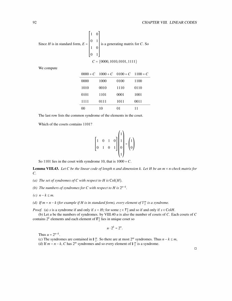
92 CHAPTER VIII. LINEAR CODES
Since H is in standard form, E =
⎡⎢⎢⎢⎢⎢⎢⎢⎢⎢⎢⎢⎣
1 0
0 1
1 0
0 1
⎤⎥⎥⎥⎥⎥⎥⎥⎥⎥⎥⎥⎦
is a generating matrix for C. So
C = 0000,1010,0101,1111
We compute
0000 +C 1000 +C 0100 +C 1100 +C
0000 1000 0100 1100
1010 0010 1110 0110
0101 1101 0001 1001
1111 0111 1011 0011
00 10 01 11
The last row lists the common syndrome of the elements in the coset.
Which of the cosets contains 1101?
⎡⎢⎢⎢⎢⎢⎣
1 0 1 0
0 1 0 1
⎤⎥⎥⎥⎥⎥⎦
⎛⎜⎜⎜⎜⎜⎜⎜⎜⎝
1
1
0
1
⎞⎟⎟⎟⎟⎟⎟⎟⎟⎠
=⎛⎜⎝
1
0
⎞⎟⎠
So 1101 lies in the coset with symdrome 10, that is 1000 +C.
Lemma VIII.43. Let C be the linear code of length n and dimension k. Let H be an m × n-check matrix forC.
(a) The set of syndromes of C with respect to H is Col(H).
(b) The numbers of syndromes for C with respect to H is 2n−k.
(c) n − k ≤ m.
(d) If m = n − k (for example if H is in standard form), every element of Fm2 is a syndrome.
Proof. (a) s is a syndrome if and only if s = Hz for some z ∈ Fn2 and so if and only if s ∈ ColH.
(b) Let u be the numbers of syndromes. by VIII.40 u is also the number of cosets of C. Each cosets of Ccontains 2k elements and each element of Fn
2 lies in unique coset so
u ⋅ 2k = 2n.
Thus u = 2n−k.(c) The syndromes are contained in Fm
2 . So there are at most 2m syndromes. Thus n − k ≤ m,(d) If m = n − k, C has 2m syndromes and so every element of Fm
2 is a syndrome.

VIII.5. DECODING LINEAR CODES 93
Remark VIII.44. Let H be an m × n-matrix in F2. Then dim NulH + dim ColH = n.
Proof. Put k = dim NulH. By VIII.43 ∣ColH∣ is equal to the number of syndromes of NulH and so equal to2n−k. Thus dim ColH = n − k = n − dim NulH.
Definition VIII.45. Let C be linear code with an m×n check matrix H. A syndrome look-up table for C withrespect to H is a function
τ ∶ Fm2 → F
n2
such that for all syndrome s of H,
(i) τ(s) has syndrome s,
(ii) τ(s) is a vector of minimal weight in τ(s) +C.
Note that (i) and (ii) just mean that τ(s) is a of minimal weight among the vectors with syndrome s.
Definition VIII.46. Let C be linear code of length n with check matrix H and τ a syndrome look-up table forC with respect to H. Then the function
σ ∶ Rn → C, z→ z + τ(Hz)
is called the decision rule for C with respect to H and τ.
Note here that by definition of a syndrome table τ(Hz) has syndrome Hz and so by VIII.40 z+τ(Hz) ∈ C.So this is well-defined.
Lemma VIII.47. Let C be linear code of length n with check matrix H, τ a syndrome look-up table for Cwith respect to H and σ the corresponding decision rule. Then σ is a Minimum Distance Rule
Proof. Let z ∈ Rn and c ∈ C. Put s = Hz. Be definition of τ, τ(s) has syndrome s. Since also z has syndromes, we conclude from VIII.40 that z + c ∈ z +C = τ(s) +C. By definition of τ, τ(s) is of minimal weight inτ(s) +C. So
wt(z + c) ≤ wt(τ(s)).
We compute
d(z, σ(z)) = d(z, z + τ(s)) = wt(z + (z + τ(s)) = wt(τ(s)) ≥ wt(z + c) = d(z, c).
Algorithm VIII.48. Let C be linear code with an m× n check matrix H. Choose an ordering z1, . . . , z2n ofF
n2 such that wt(zi) ≤ wt(z j) for all 1 ≤ i < j ≤ 2n. Define functions τl ∶ S l → F
m2 inductively as follows:
For l = 0 let S 0 = ∅ and τ0 = ∅.Suppose l > 0 and τl−1 has been defined. Compute sl = Hzl.
• If sl ∈ S l−1, put τl = τl−1
• If sl ∉ S l, put S l = S l−1 ∪ sl and extend τl−1 to a function τl on S l by τl(sl) = zl.
Stop the algorithm if l = 2n or ∣S l∣ = 2m.The last τl is a syndrome look up table for C with respect to H.

94 CHAPTER VIII. LINEAR CODES
Example VIII.49. Let C be the code with check matrix.
H =
⎡⎢⎢⎢⎢⎢⎢⎢⎢⎣
1 0 1 0 0
1 1 0 1 0
0 1 0 0 1
⎤⎥⎥⎥⎥⎥⎥⎥⎥⎦
Construct a syndrome look-up table τ and compute σ(11001), where σ is the decision rule for C withrespect to H and τ.
zl
00000
10000
01000
00100
00010
00001
11000
10100
10010
10001
sl000
110
011
100
010
001
101
010
100
111
∣S l∣ 1 2 3 4 5 6 7 − − 8
⎡⎢⎢⎢⎢⎢⎢⎢⎢⎣
1 0 1 0 0
1 1 0 1 0
0 1 0 0 1
⎤⎥⎥⎥⎥⎥⎥⎥⎥⎦
⎛⎜⎜⎜⎜⎜⎜⎜⎜⎜⎜⎜⎝
1
1
0
0
1
⎞⎟⎟⎟⎟⎟⎟⎟⎟⎟⎟⎟⎠
=
⎛⎜⎜⎜⎜⎝
1
0
0
⎞⎟⎟⎟⎟⎠
τ(100) = 00100
and so
σ(11001) = 11001 + 00100 = 11101
To double check
⎡⎢⎢⎢⎢⎢⎢⎢⎢⎣
1 0 1 0 0
1 1 0 1 0
0 1 0 0 1
⎤⎥⎥⎥⎥⎥⎥⎥⎥⎦
⎛⎜⎜⎜⎜⎜⎜⎜⎜⎜⎜⎜⎝
1
1
1
0
1
⎞⎟⎟⎟⎟⎟⎟⎟⎟⎟⎟⎟⎠
=
⎛⎜⎜⎜⎜⎝
0
0
0
⎞⎟⎟⎟⎟⎠

Chapter IX
Algebraic Coding Theory
IX.1 Classification and properties of cyclic codesDefinition IX.1. A code C ⊆ Fn
2 is called cyclic if
(a) C is linear, and
(b) ana1 . . .an−1 ∈ C for all a = a1 . . .an ∈ C.
Example IX.2. Which of following codes are cyclic?
(a) 000,100,111,011.
(b) 000,100,010,001
(c) 000,1010,0101,1111
(a): Not cyclic, since 100 is in the code, but 010 is not.(b): Not cyclic, since its not linear: 100 and 010 are in the code, but 100 + 010 = 110 is not.(c): Is cyclic.
Definition IX.3. An ideal in a ring R is a subset S of R such that
(a) 0 ∈ S .
(b) If s, t ∈ S then s + t ∈ S .
(c) If a ∈ R and s ∈ S , then as ∈ S and sa ∈ S .
Example IX.4. The set of even integers is an ideal in the integers.
Indeed 0 is even. Sums of even integers are even and any multiple of an even integer is even.
Lemma IX.5. Let F be a field and f ,g ∈ F[x] with g ≠ 0. Then there exists uniquely determined q, r ∈ F[x]with
f = qh + r and deg r < deg h
r is called the remainder of f when divided by h.
95

96 CHAPTER IX. ALGEBRAIC CODING THEORY
Proof. We first prove the existence of q and r by induction on deg f . Note that f = 0h+ f , so if deg f < deg h,we can choose q = 0 and r = f .
Suppose now that deg f ≥ h. Let f = ∑mi=0 aixi and h = ∑n
i=0 bixi with am ≠ 0 ≠ bn. Then m = deg h ≥deg h = n. Put
f = f − bm
anxm−nh.
Observe that the coefficient of xm in f is bm − bman
an = bm − bm = 0. Hence deg f < m = deg f . So byinduction, there exist q, r ∈ F[x] with
f = qh + r and deg r < deg h
We have
f = f + bm
anxm−nh = qh + r + bm
anxm−nh = (q + bm
anxm−n)h + r.
So we can choose q = q + bman
xm−n and r = r.
This shows this existence of q and r. For the uniqueness suppose
f = qh + r = q∗h + r∗, deg r < deg h and deg r∗ < deg h
for some q,q∗, r, r∗ ∈ F[x]. Then
(q − q∗)h = r∗ − r.
By A.8, deg(r∗ − r) ≤ max(deg r,deg r∗) < deg h and so deg(q − q∗)h < deg h. Hence A.8 shows thatq − q∗ = 0 and so also r∗ − r = (q − q∗)h = 0h = 0.
Hence q = q∗ and r = r∗. So q and r are unique.
Definition IX.6. Let F be a field and h ∈ F[x] with h ≠ 0. Let f ,g ∈ F[x].
f is the remainder of f when divided by h.
Define an addition ⊕ and multiplication ⊙ on F[x] as follows:
f ⊕ g = f + g
and
f ⊙ g = f g.
For n ∈ N, define f⊙n inductively by
f⊙0 = 1 and f⊙(n+1) = f⊙n ⊙ f .
LetF
h[x] = f ∈ F[x] ∣ deg f < deg h
(Fh[x],⊕,⊙) is called the ring of polynomials modulo h with coefficients in F.
Example IX.7. Determine the addition and multiplication in Rx2+1[x].

IX.1. CLASSIFICATION AND PROPERTIES OF CYCLIC CODES 97
Since deg x2 + 1 = 2 we have Rx2+1[x] = a + bx ∣ a,b ∈ R. We compute
(a + bx)⊕ (c + dx) = (a + c) + (b + dx)
and
(a + bx)⊙ (c + dx) = ac + adx + bcx + bdx2
= (ac − bd) + (ad + bc)x + bd(x2 + 1)= (ac − bd) + (ad + bc)x
So Rx2+1[x] has the same addition and multiplication as the ring of complex numbers
C = a + bi ∣ a,b ∈ R.
Lemma IX.8. Let F be a field and h ∈ F[x] with h ≠ 0. Let f ,g ∈ Fh[x] and a ∈ F.
(a) f = f .
(b) f ⊕ g = f + g
(c) a⊙ f = a f .
Proof. (a) f = 0h + f and deg f < deg h. So f is the remainder of f when divided by h.(b) Observe that deg( f + g) ≤ max(deg f ,deg g) < deg h and so by (a) f + g = f + g.(c) Since deg a f ≤ deg f < deg h, (a) gives a f = a f .
Remark IX.9. Let F be a field and h ∈ F[x] with h ≠ 0. Then Fh[x] is vector space over F.
Definition IX.10. Let R be a commutative ring and a,b ∈ R. We say that a divides b and write a ∣ b if b = rafor some r ∈ R.
Lemma IX.11. Let F be a field and h ∈ F[x] with h ≠ 0. Let f ,g ∈ F[x], a ∈ F and n ∈ N. Then
(a) f ∈ Fh[x].
(b) 0⊕ f = 1⊙ f = f = f = f ⊙ 1 = f ⊕ 0
(c) f ⊕ g = f + g = f + g = f ⊕ g = f ⊕ g = f ⊕ g
(d) f ⊙ g = f g = f g = f ⊙ g = f ⊙ g = f ⊙ g
(e) f n = f⊙n = ( f )⊙n = ( f )n
(f) − f = − f .
(g) f = 0 if and only if h divides f .
(h) f = g if and only if h divides g − f .
(i) a⊙ f = a f = a f

98 CHAPTER IX. ALGEBRAIC CODING THEORY
Proof. Recall first that by definition of the remainder f = ph + f and g = qh + g for some p,q ∈ F[x]. Alsodeg f < deg h and deg g < deg h.
(a) Since deg f < deg h, f ∈ Fh[x].
(b) 1⊙ f = 1 f = f = 0 + f = 0⊕ f . Since f ∈ Fh[x], IX.8(a) gives f = f .(c) We compute
f + g = (ph + f ) + (qh + g) = (p + q)h + ( f + g)
Note that f + g has degree less than h and so f + g is the remainder of f + g when divided by h. Hencef ⊕ g = f + g = f + g.
By IX.8(b), f ⊕ g = f + g. The remaining parts of (c) now follow from f = f and g = g.(d) By definition f g = th + f g for some t ∈ F[x] and deg f g < deg h. We have
f g = (ph + f )(qh + g) = (phq + f q + pg)h + f g = (phq + f q + pg + t)h + f g
So f g is the remainder of f g when divided by h. Hence f ⊙ g = f g = f g. (d) is now readily verified.(e) For n = 0 all four expression are equal to 1.Suppose (e) holds for n. Then using (d)
f (n+1) = f n f = f n ⊙ f = f n ⊙ f = f⊙n ⊙ f = f⊙(n+1)
( f )⊙(n+1) = ( f )⊙n ⊙ f = f n ⊙ f = f n ⊙ f
and
( f )(n+1) = ( f )nf = f⊗n f = f⊗n ⊙ f
(f) − f = −ph + (− f ) and so − f is the remainder of f when divided by h.(g) h divides f if and only if f = sh for some s ∈ F[x] and so if and only if f = sh + 0 for some s ∈ F[x].
Since deg 0 < deg h, this holds if and only if 0 is the remainder of f when divided by 0.(h) f = g if and only if f − g = 0 and if and only if f − g = 0. So (h) follow from (g).(i) By (d), a⊙ f = a f = a⊙ f and by IX.8(c) a⊙ f = a f .
Lemma IX.12. Let F be a field, 0 ≠ h ∈ F[x] and I ⊆ Fh[x]. Then I is an ideal in Fh[x] if and only if I is anF-subspace of Fh[x] and x⊙ f ∈ I for all f ∈ I.
Proof. Let f ,g ∈ I and a ∈ F.Ô⇒: Suppose that I is an ideal in Fh[x]. Then by definition of an ideal, 0 ∈ I and f + g ∈ I. Also since
a ∈ Fh[x]), a f = a ⊙ f ∈ I. Thus I is an F-subspace of Fh[x]. Also x ⊙ f = x ⊙ f ∈ I and so the forwarddirection is proved.⇐Ô: Suppose I is an F-subspace of Fh[x] and x ⊙ f ∈ I for all f ∈ I. Then by definition of a subspace
0 ∈ I and f + g ∈ I.We claim that xi ⊙ f ∈ I for all i ∈ N. x0 ⊙ f = 1 ⊙ f = f and so the claim holds for i = 0. Suppose
inductively that xi ⊙ f ∈ I. Then by assumption also x⊙ (xi ⊙ f ) ∈ I and hence
xi+1 ⊙ f = xi+1 f = x(xi f ) = x⊙ xi f = x⊙ (xi ⊙ f ) ∈ I.
So indeed xi ⊙ f ∈ I for all i ∈ N and f ∈ I.Let g ∈ Fh[x]. Then g = ∑n
i=0 aixi for some ai ∈ F2 and so
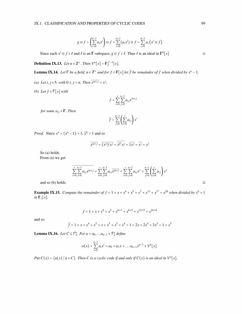
IX.1. CLASSIFICATION AND PROPERTIES OF CYCLIC CODES 99
g⊙ f = (n−1
∑i=0
aixi)⊙ f =n−1
∑i=0
(aixi)⊙ f =n−1
∑i=0
ai (xi ⊙ f )
Since each xi ⊙ f ∈ I and I is an F-subspace, g⊙ f ∈ I. Thus I is an ideal in Fh[x].
Definition IX.13. Let n ∈ Z+. Then Vn[x] = Fxn−12 [x].
Lemma IX.14. Let F be a field, n ∈ Z+ and for f ∈ F[x] let f be remainder of f when divided by xn − 1.
(a) Let i, j ∈ N with 0 ≤ j < n. Then xni+ j = x j.
(b) Let f ∈ F[x] with
f =r
∑i=0
n−1
∑j=0
ai jxin+ j
for some ai j ∈ F. Then
f =n−1
∑j=0
(r
∑i=0
ai j) xi
Proof. Since xn = (xn − 1) + 1, xn = 1 and so
xni+ j = (xn)ix j = xnix j = 1x j = x j = x j
So (a) holds.From (a) we get
r
∑i=0
n−1
∑j=0
ai jxin+ j =r
∑i=0
n−1
∑j=0
ai jxin+ j =r
∑i=0
n−1
∑j=0
ai jx j =n−1
∑j=0
(r
∑i=0
ai j) x j
and so (b) holds.
Example IX.15. Compute the remainder of f = 1 + x + x4 + x5 + x7 + x11 + x17 + x28 when divided by x6 + 1in F2[x].
f = 1 + x + x4 + x5 + x6+1 + x6+5 + x12+5 + x24+4
and sof = 1 + x + x4 + x5 + x + x5 + x5 + x4 = 1 + 2x + 2x4 + 3x5 = 1 + x5
Lemma IX.16. Let C ⊆ Fn2. For a = a0 . . .an−1 ∈ Fn
2 define
a(x) =n−1
∑i=0
aixi = a0 + a1x + . . .an−1xn−1 ∈ Vn[x].
Put C(x) = a(x) ∣ a ∈ C. Then C is a cyclic code if and only if C(x) is an ideal in Vn[x].

100 CHAPTER IX. ALGEBRAIC CODING THEORY
Proof. Note that 0 ∈ C if and only if 0 = 0(x) ∈ C(x). Let a,b ∈ C. Then a + b ∈ C if and only if(a+ b)(x) ∈ C(x) and so if and only if a(x)+ b(x) ∈ C(x). Thus C is a subspace of Fn
2 if and only if C(x) isa subspace of Vn[x].
Put a = an−1a0 . . .an−2. Then
x⊙ a(x) = xn−1
∑i=0
aixi =n−1
∑i=0
aixi+1 = an−1 + a0x + . . . + an−2xn−1 = a(x)
Thus a ∈ C if and only if x⊙ a(x) ∈ C(x). So by IX.12 C is cyclic if and only if C(x) is an ideal.
Definition IX.17. Let R be a commutative ring and a ∈ R. Define ⟨a⟩ = ra ∣ r ∈ R. ⟨a⟩ is called the ideal inR generated by a.
Lemma IX.18. Let R be a commutative ring and a ∈ R.
(a) ⟨a⟩ is an ideal in R.
(b) ⟨a⟩ ⊆ I for any ideal I of R with a ∈ I.
Proof. (a) We have 0 = 0a ∈ ⟨a⟩. Also for any r, s ∈ R, ra + sa = (r + s)a ∈ ⟨a⟩ and s(ra) = (sr)a ∈ ⟨a⟩.(b) By definition of an ideal, ra ∈ I for all r ∈ R and so ⟨a⟩ ⊆ I.
Lemma IX.19. Let F be a field, h ∈ F[x] with h ≠ 0 and f ∈ Fh[x]. Let ⟨ f ⟩ be the ideal in Fh[x] generatedby f . Then
(a) ⟨ f ⟩ is the F-subspace of Fh[x] spanned by
1⊙ f , x⊙ f , . . . , xn−1 ⊙ f
where n = deg h.
(b) ⟨ f ⟩ = g⊙ f ∣ g ∈ F[x].
Proof. (a) Let g = ∑n−1i=0 aixi ∈ Fh[x]. Then
g⊙ f = a0(1⊙ f ) + a1(x⊙ f ) + . . . + an−1(xn−1 ⊙ f )
and so the elements of ⟨ f ⟩ are exactly the F-linear combinations of 1⊙ f , x⊙ f , . . . , xn−1 ⊙ f .(b)
⟨ f ⟩ = g⊙ f ∣ g ∈ Fh[x] = g⊙ f ∣ g ∈ F[x] = g⊙ f ∣ g ∈ F[x].
Example IX.20. Find the ideal in V3[x] generated by f = 1 + x2 and determined the corresponding cycliccode.
1⊙ (1 + x2) = 1 + x2
x⊙ (1 + x2) = x + x3 = x + 1
x2 ⊙ (1 + x2) = x2 + x4 = x + x2
Note that (1 + x2) + (1 + x) = x2 + x. So

IX.1. CLASSIFICATION AND PROPERTIES OF CYCLIC CODES 101
⟨x2 + 1⟩ = 0,1 + x2,1 + x, x + x2.
The corresponding cyclic code is
000,101,110,011
Lemma IX.21. Let F be a field and f ,g, t ∈ F[x] with t ≠ 0. Then f ∣ g if and only if f t ∣ gt.
Proof.
f t ∣ gt
⇐⇒ gt = f tl for some l ∈ F[x]⇐⇒ gt − f tl = 0 for some l ∈ F[x]⇐⇒ (g − f l)t = 0 for some l ∈ F[x]⇐⇒ g − f l = 0 for some l ∈ F[x]⇐⇒ g = f l for some l ∈ F[x]⇐⇒ f ∣ g
Lemma IX.22. Let F be a field, h ∈ F[x] with h ≠ 0 and I an ideal in Fh[x]. Let g ∈ F[x] be of minimaldegree with g ∈ I and g ≠ 0.
(a) Let f ∈ F[x]. Then f ∈ I if and only if g divides f in F[x].
(b) I = ⟨g⟩.
(c) g divides h in F[x] and so h = tg for some t ∈ F[x].
(d) Let f , f ∗ ∈ F[x]. Then f ⊙ g = f ∗ ⊙ g if and only if t divides f ∗ − f .
(e) Let k = deg t. Then I = sg ∣ s ∈ F[x],deg s < k.
(f) (g, xg, x2g, . . . , xk−1g) is an F-basis for I.
(g) dimF I = k.
(h) Let f ∈ F[x]. Then f ∈ I if and only if f ⊙ t = 0.
(i) Suppose that h = xn − 1 and let f ∈ Fh[x]. Then f ∈ I if and only if the coefficient of xi in f t is 0 for allk ≤ i < n.
Proof. Let n = deg h. Since h = 0 ∈ I, deg g ≤ deg h(a) Let f = qg + r with q, r ∈ F[x] and deg r < deg g. If g ∣ f , then f = qg and so f = q⊙ g ∈ I.Suppose f ∈ I. Since deg r < deg g ≤ deg h, we have r = r = f − qg = f ⊕ −q⊙ g ∈ I. The minimal choice
of deg g shows that r = 0 and so g ∣ f .
(b) Let f ∈ I. Then deg f < n and so f = f ∈ I. Thus by (a), f = eg for some e ∈ F[x]. Thereforef = f = e⊙ g and f ∈ ⟨g⟩. Since g ∈ I, IX.18(b) shows ⟨g⟩ ⊆ I and thus I = ⟨g⟩.
(c) Note that h = 0 ∈ I and so by (a) , h = tg for some t ∈ F[x].
(d) We have

102 CHAPTER IX. ALGEBRAIC CODING THEORY
f ⊙ g = f ∗ ⊙ g
⇐⇒ f g = f ∗g − definition of ⊙⇐⇒ h divides f g − f ∗g − IX.11(h)⇐⇒ tg divides ( f − f ∗)g − (c)⇐⇒ t divides f − f ∗ − IX.21
(e) Let f ∈ Fh[x] and let s be the remainder of f when divided by t. Then t divides f − s and so by (d),f ⊙ g = f ⊙ g = s⊙ g. Note that deg sg < k + (n − k) = n and so s⊙ g = sg = sg. Hence
I = ⟨g⟩ = f ⊙ g ∣ f ∈ Fh[x] = sg ∣ s ∈ F[x],deg s < k
(f) Note that deg g = n − k. Let s ∈ F[x] with deg r < k and let s = ∑k−1i=0 aixi. Then
(∗) sg =k−1
∑i=0
aixig.
Together with (e) we see that I is the set of F-linear combinations of (g, xg, x2g, . . . , xk−1g).If (a0, . . . ,ak−1) ≠ 0, then s ≠ 0 and sg ≠ 0. By (*) ∑k−1
i=0 aixi ≠ 0 and so (g, xg, x2g, . . . xk−1g) is linearlyindependent.
(g) follows immediately from (f).(h)
f ∈ I
⇐⇒ g ∣ f − (a)⇐⇒ gt ∣ f t − IX.21⇐⇒ h ∣ f t − (c)
⇐⇒ f t = 0 − IX.11(h)⇐⇒ f ⊙ t = 0 − definition of ⊙
(i) Let f ∈ Fh[x] and write f = qg + r with deg r < deg g = n − k. By (a),
f = f ∈ I ⇐⇒ r = 0.
Since deg f < n and deg g = n − k, we have
deg q < k
Also
deg rt = deg r + deg t < (n − k) + k = n.
Note that r = 0 if and only if deg rt < deg t, that is if only if deg rt < k. Since deg rt < n, this gives
r = 0 ⇐⇒ the coefficient of xi in rt is 0 for k ≤ i < n

IX.1. CLASSIFICATION AND PROPERTIES OF CYCLIC CODES 103
We compute
f t = (qg + r)t = qgt + rt = qh + rt = q ⋅ (xn − 1) + rt = qxn − q + rt
Let k ≤ i < n. Since i < n, the coefficient of xi in qxn is 0. Since i ≥ k and deg q < k, the coefficient of xi inq also 0. Thus the coefficent of xi in f t is the same as the coefficient of xi in rt. Hence (i) holds.
Definition IX.23. Let F be a field.
(a) Let 0 ≠ f = ∑mi=0 aixi ∈ F[x] with am ≠ 0. Then am is called the leading coefficient of f . If f = 0, we call 0
the leading coefficient of f . We denote the leading coefficient of f be lead( f ).
(b) A monic polynomial is a polynomial with leading coefficient 1.
(c) Let 0 ≠ h ∈ F[x] and I an ideal in Fh[x]. Let g ∈ F[x] be a monic polynomial of minimal degree withg ∈ I. Then g is called the canonical generator for I. (If I ≠ 0, then g is the monic polynomial of minimaldegree in I, and if I = 0, g = 1
lead(h)h).
Lemma IX.24. Let F be a field and 0 ≠ h ∈ F[x].
(a) Let I an ideal in Fh[x]. Then the canonical generator of I is unique.
(b) Let g ∈ F[x] be monic. Then g is the canonical generator for the ideal ⟨g⟩ in Fh[x] if and only if g ∣ h.
Proof. (a) Let g1 and g2 be canonical generators of I. Then deg g1 = deg g2 and g1 and g2 are monic. Thusdeg g1 − g2 < deg g1. Also g1 − g2 = g1 − g2 ∈ I and so by minimal choice of deg gi, g1 − g2 = 0 and g1 = g2.
(b) If g is the canonical generator for ⟨g⟩, then IX.22 shows that g ∣ h.Conversely suppose that g ∣ h and let g be the canonical generator for ⟨g⟩. Since g = ⟨g⟩,
g = f ⊙ g = f g
for some f ∈ Fh[x]. Thus IX.11 shows that h divides g − f g. Thus g − f g = kh for some k ∈ F[x]. Sog = f g + kh. Since g ∣ h this shows that g ∣ g. Thus deg g ≤ deg g. The minimal choice of deg g now showsthat deg g = deg g and so also g is a canonical generator of ⟨g⟩.
Definition IX.25. Let a = a0 . . .an−1 ∈ Fn2. For 0 ≤ i < n define
a(i) = an−i . . .an−1a0a1 . . .an−1−i
a(i) is called the cyclic i-shift of a.⟨a⟩ is the linear subspace of Fn
2 spanned by a(0),a(1), . . . ,a(n−1). ⟨a⟩ is called the cyclic code generatedby a.
Corollary IX.26. Let C ⊆ Fn2 be cyclic code. Then there exists a ∈ C with C = ⟨a⟩.
Proof. Let C(x) be the ideal of Vn[x] correponding to C. Then C(x) = ⟨g⟩ for some g ∈ V[x]. Let a ∈ Cbe the codeword corresponding to g. Then a(i) corresponds to xi ⊙ g and since C(x) is spanned by xi ⊙ g,0 ≤ i < n, C is spanned by a(i).
Example IX.27. Determine the cyclic code generated by 0110 and find the canonical generator for thecorresponding ideal in V4[x].

104 CHAPTER IX. ALGEBRAIC CODING THEORY
The cyclic shifts of 0110 are
0110,0011,1001,1100
Since 1001 = 1100 + 0110 + 0011, ⟨1100⟩ is spanned by
1100,0110,0011.
Sums of 0 of these word:
0000
Sums of two of these words:
1010,0101,1111.
Sum of all three:
1001.
So
⟨1100⟩ = 0000,1100,0110,0011,1001,1010,0101,1111.
The non-zero codeword with the most trailing zeros is 1100. So the canonical generator is 1 + x.
Theorem IX.28. Let C ⊆ Fn2 be a cyclic code. Let g be the canonical generator of the ideal C(x) in Vn[x].
Let h ∈ F[x] with gh = xn − 1. Put k = deg h and m = n − k = deg g.
(a) The n × k matrix
E =
⎡⎢⎢⎢⎢⎢⎢⎢⎢⎢⎢⎢⎢⎢⎢⎢⎢⎢⎢⎢⎢⎢⎢⎢⎢⎢⎢⎢⎢⎢⎢⎢⎢⎢⎢⎢⎣
c0 0 0 . . . 0 0
c1 c0 0 . . . 0 0
⋮ c1 c0 . . . ⋮ ⋮
⋮ ⋮ c1 . . . 0 ⋮
cm−1 ⋮ ⋮ . . . c0 0
cm cm−1 ⋮ . . . c1 c0
0 cm cm−1 . . . ⋮ c1
0 0 cm . . . ⋮ ⋮
⋮ 0 0 . . . cm−1 ⋮
⋮ ⋮ ⋮ . . . cm cm−1
0 0 0 . . . 0 cm
⎤⎥⎥⎥⎥⎥⎥⎥⎥⎥⎥⎥⎥⎥⎥⎥⎥⎥⎥⎥⎥⎥⎥⎥⎥⎥⎥⎥⎥⎥⎥⎥⎥⎥⎥⎥⎦
is a generating matric for C.

IX.1. CLASSIFICATION AND PROPERTIES OF CYCLIC CODES 105
(b) The m × n matrix
H =
⎡⎢⎢⎢⎢⎢⎢⎢⎢⎢⎢⎢⎢⎢⎢⎢⎢⎢⎢⎣
hk hk−1 hk−2 . . . h1 h0 0 0 . . . 0
0 hk hk−1 . . . h2 h1 h0 0 . . . 0
0 0 hk . . . h3 h2 h1 h0 . . . 0
⋮ ⋮ ⋮ ⋮ ⋮ ⋮ ⋮ ⋮ ⋮ ⋮
0 0 0 . . . hk . . . . . . h1 h0 0
0 0 0 . . . 0 hk . . . h2 h1 h0
⎤⎥⎥⎥⎥⎥⎥⎥⎥⎥⎥⎥⎥⎥⎥⎥⎥⎥⎥⎦
is a check matrix for C.
Proof. (a) By IX.22 C(x) is spanned by the polynomials xig, 0 ≤ i < k. Thus C is spanned by the cyclic shiftsc(i), 0 ≤ i < k. Since the columns of E are the c(i), (a) holds.
(b) Let d = d0d1 . . .dn−1 ∈ Fn2 and d(x) the corresponding polynomial. By IX.22, d(x) ∈ C(x) if and only
if the coefficent as of xs in h ⋅ d(x) is equal to 0 for all k ≤ s < n. We compute
as =s
∑l=0
hlds−l
Since deg h = k, hl = 0 for l ≥ k. Put i = s − k. Then 0 ≤ i < n − k = m and
as =k
∑l=0
hlds−l = hkdi + hk−1di+1 + . . . + h1ds−1 + h0ds
Hence
ak = hkd0 + hk−1d1 + hk−2d2 + . . . + h1dk−1 + h0dk
ak+1 = hkd1 + hk−1d2 + . . . + h2dk−1 + h1dk + h0dk+1
ak+2 = hkd2 + . . . + h3dk−1 + h2dk + h1dk+1 + h0dk+2
⋮ ⋮ ⋱ ⋱ ⋱ ⋱ ⋱ ⋱ ⋱ ⋱ ⋱ ⋱an−2 = hkdn−k−2 + . . . + . . . + h1dn−3 + h0dn−2
an−1 = hkdn−k−1 + . . . + h2dn−3 + h1dn−2 + h0dn−1
So ak+i = 0 for 0 ≤ i < m if and only if Hd = 0. So H is indeed a check matrix for C.
Example IX.29. Find a generating and a check matrix for the cyclic code C of length 7 with canonicalgenerator g = 1 + x2 + x3 + x4. Is 1001011 in the code?
We have n = 7, m = deg g = 4 and k = n −m = 7 − 4 = 3. Since g = 1 + x2 + x3 + x4 the first column of E is1011100. So
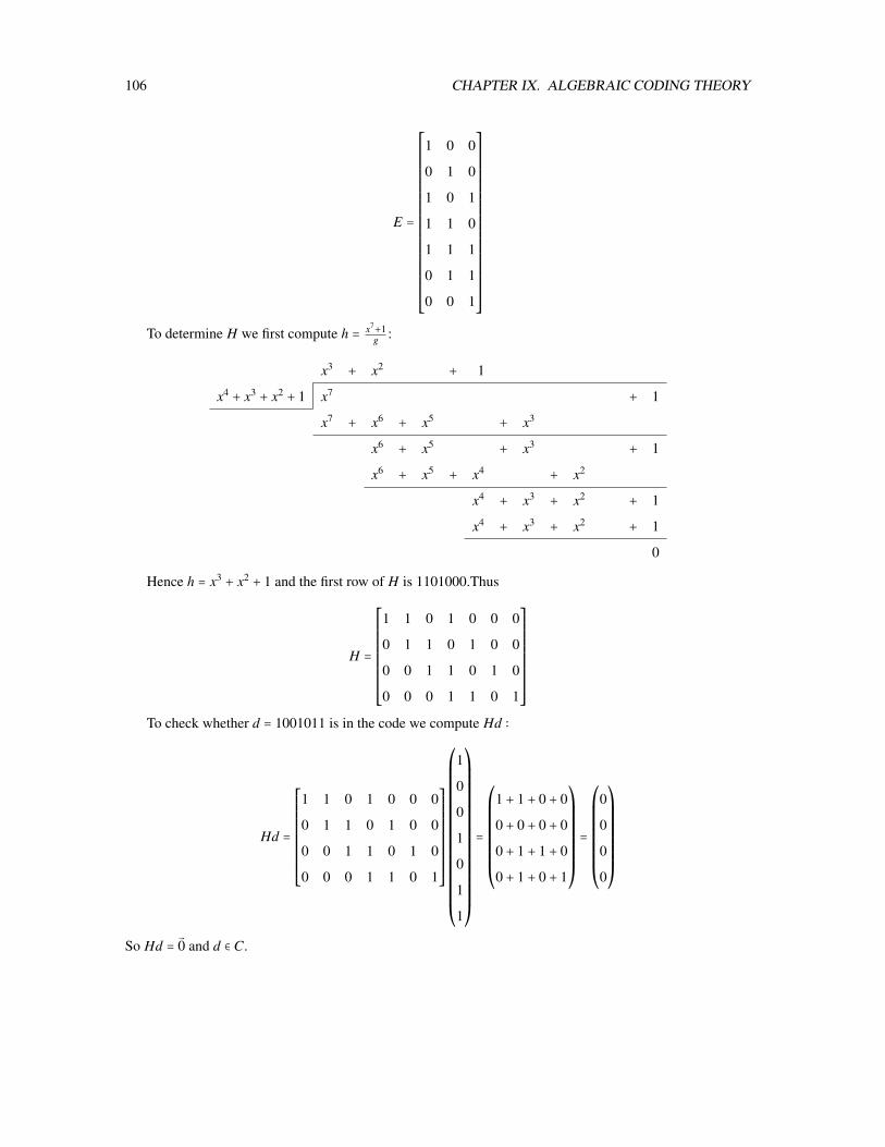
106 CHAPTER IX. ALGEBRAIC CODING THEORY
E =
⎡⎢⎢⎢⎢⎢⎢⎢⎢⎢⎢⎢⎢⎢⎢⎢⎢⎢⎢⎢⎢⎢⎢⎣
1 0 0
0 1 0
1 0 1
1 1 0
1 1 1
0 1 1
0 0 1
⎤⎥⎥⎥⎥⎥⎥⎥⎥⎥⎥⎥⎥⎥⎥⎥⎥⎥⎥⎥⎥⎥⎥⎦To determine H we first compute h = x7+1
g :
x3 + x2 + 1
x4 + x3 + x2 + 1 x7 + 1
x7 + x6 + x5 + x3
x6 + x5 + x3 + 1
x6 + x5 + x4 + x2
x4 + x3 + x2 + 1
x4 + x3 + x2 + 1
0
Hence h = x3 + x2 + 1 and the first row of H is 1101000.Thus
H =
⎡⎢⎢⎢⎢⎢⎢⎢⎢⎢⎢⎢⎣
1 1 0 1 0 0 0
0 1 1 0 1 0 0
0 0 1 1 0 1 0
0 0 0 1 1 0 1
⎤⎥⎥⎥⎥⎥⎥⎥⎥⎥⎥⎥⎦To check whether d = 1001011 is in the code we compute Hd ∶
Hd =
⎡⎢⎢⎢⎢⎢⎢⎢⎢⎢⎢⎢⎣
1 1 0 1 0 0 0
0 1 1 0 1 0 0
0 0 1 1 0 1 0
0 0 0 1 1 0 1
⎤⎥⎥⎥⎥⎥⎥⎥⎥⎥⎥⎥⎦
⎛⎜⎜⎜⎜⎜⎜⎜⎜⎜⎜⎜⎜⎜⎜⎜⎜⎜⎜⎝
1
0
0
1
0
1
1
⎞⎟⎟⎟⎟⎟⎟⎟⎟⎟⎟⎟⎟⎟⎟⎟⎟⎟⎟⎠
=
⎛⎜⎜⎜⎜⎜⎜⎜⎜⎝
1 + 1 + 0 + 0
0 + 0 + 0 + 0
0 + 1 + 1 + 0
0 + 1 + 0 + 1
⎞⎟⎟⎟⎟⎟⎟⎟⎟⎠
=
⎛⎜⎜⎜⎜⎜⎜⎜⎜⎝
0
0
0
0
⎞⎟⎟⎟⎟⎟⎟⎟⎟⎠
So Hd = 0 and d ∈ C.

IX.2. DEFINITION OF A FAMILY OF BCH CODES 107
We could also have observed that d is the sum of the first and last column of E and so d ∈ C.
IX.2 Definition of a family of BCH codes
Irreducible polynomialsDefinition IX.30. Let F be a field and h ∈ F[x]. Then h is called irreducible if
(i) deg h > 0.
(ii) if h = f g for some f ,g ∈ F[x], then deg f = 0 or deg g = 0.
Remark IX.31. Let F be a field and h ∈ F[x]. Then h is irreducible if and only
(i) deg h > 0.
(ii) If f ∣ h for some f ∈ F[x], then deg f = 0 or deg f = h.
Proof. We may assume that deg h > 0.Suppose first that h is irreducible and let f ∈ F[x] with f ∣ h. Then h = f g for some g ∈ F[x]. Since h is
irreducible, deg f = 0 or deg g = 0. If deg g = 0, then deg f = deg h − deg g = deg f .Suppose next that (ii) holds and that f ,g ∈ F[x] with h = f g. Then f ∣ h and so deg f = 0 or deg f = deg h.
If deg f = deg h, then deg g = deg h − deg f = 0. So h is irreducible.
Lemma IX.32. Let R be a commutative ring and r ∈ R. Then sr = 1 for some s ∈ R if and only if ⟨r⟩ = R.
Proof. Suppose sr = 1 for some s ∈ R. Let t ∈ R. Then t = t1 = t(sr) = (ts)r ∈ ⟨r⟩ and so R = ⟨r⟩. Supposethat R = ⟨r⟩. Then 1 ∈ ⟨r⟩ and so 1 = sr for some s ∈ R.
Lemma IX.33. Let F be a field and let h ∈ F[x] be irreducible. Put E = Fh[x].
(a) F is a subfield of E
(b) E is a field.
(c) Let h = ∑ni=0 hixi. Then x is a root in E of the polynomial ∑n
i=0 hiyi in E[y].
Proof. (a) Let a,b ∈ F. Then a,b,a + b and ab are polynomials of degree at most 0. Since deg h > 0, we geta⊕ b = a + b and a⊙ b = ab. So F is a subfield of Fh[x].
(b) Let 0 ≠ f ∈ Fh[x] and put I = ⟨ f ⟩. Let g be the canonical generator for I. Then g divides h. Since0 ≠ f ∈ I we have g ∣ f and so deg g ≤ deg f < deg h and g ≠ 0. Since h is irreducible, this implies deg g = 0.Hence g ∈ F and g−1 is a polynomial of degree 0 with 1 = g−1g = g−1 ⋅ g. Thus by IX.32, ⟨g⟩ = Fh[x]. Since⟨ f ⟩ = I = ⟨g⟩ = Fh[x], another application of IX.32 shows that s ⋅ f = 1 for some s ∈ Fh[x]. Hence Fh[x] is afield.
(c) Let e ∈ E. Note that in E we have to use the operations ⊕ and ⊙. So e is a root of ∑ni=0 hiyi in E if and
only if
h0 ⊕ h1 ⊙ e⊕ h1 ⊙ e⊙2 ⊕ . . .⊕ hn ⊙ e⊙n = 0
and if and only if
m
∑i=0
hiei = 0
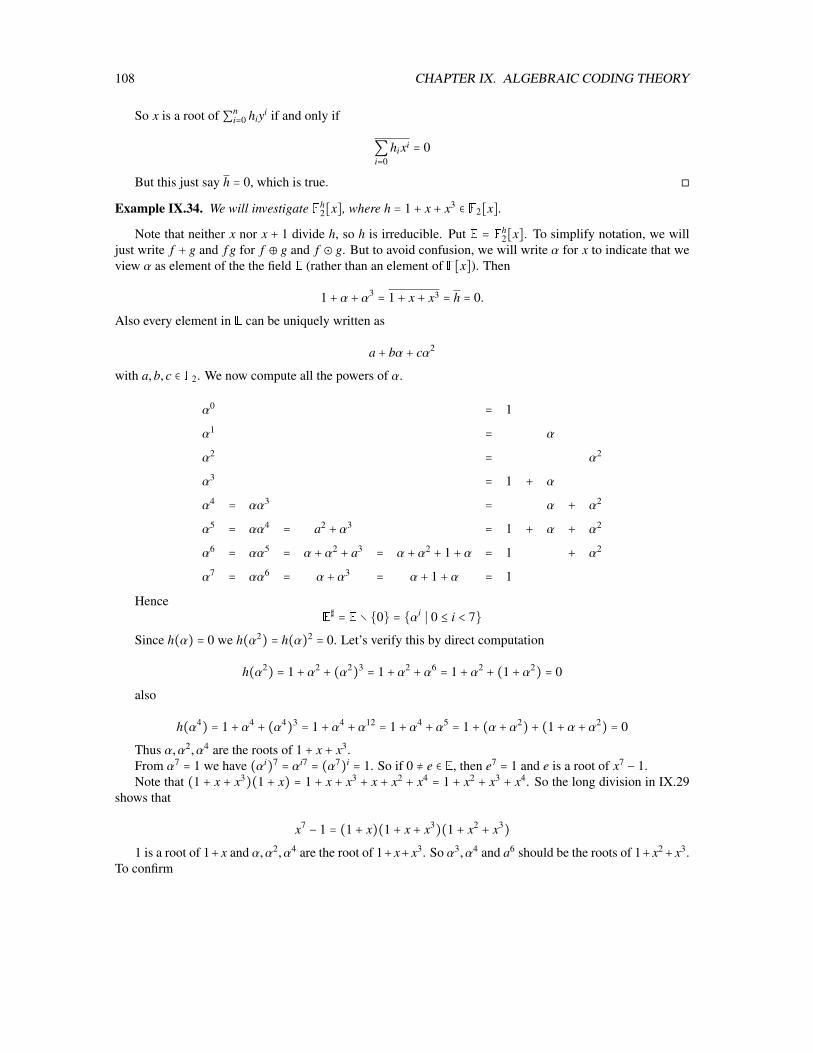
108 CHAPTER IX. ALGEBRAIC CODING THEORY
So x is a root of ∑ni=0 hiyi if and only if
∑i=0
hixi = 0
But this just say h = 0, which is true.
Example IX.34. We will investigate Fh2[x], where h = 1 + x + x3 ∈ F2[x].
Note that neither x nor x + 1 divide h, so h is irreducible. Put E = Fh2[x]. To simplify notation, we will
just write f + g and f g for f ⊕ g and f ⊙ g. But to avoid confusion, we will write α for x to indicate that weview α as element of the the field E (rather than an element of F[x]). Then
1 + α + α3 = 1 + x + x3 = h = 0.
Also every element in E can be uniquely written as
a + bα + cα2
with a,b, c ∈ F2. We now compute all the powers of α.
α0 = 1
α1 = α
α2 = α2
α3 = 1 + α
α4 = αα3 = α + α2
α5 = αα4 = a2 + α3 = 1 + α + α2
α6 = αα5 = α + α2 + a3 = α + α2 + 1 + α = 1 + α2
α7 = αα6 = α + α3 = α + 1 + α = 1
HenceE♯ = E ∖ 0 = αi ∣ 0 ≤ i < 7
Since h(α) = 0 we h(α2) = h(α)2 = 0. Let’s verify this by direct computation
h(α2) = 1 + α2 + (α2)3 = 1 + α2 + α6 = 1 + α2 + (1 + α2) = 0
also
h(α4) = 1 + α4 + (α4)3 = 1 + α4 + α12 = 1 + α4 + α5 = 1 + (α + α2) + (1 + α + α2) = 0
Thus α,α2, α4 are the roots of 1 + x + x3.From α7 = 1 we have (αi)7 = αi7 = (α7)i = 1. So if 0 ≠ e ∈ E, then e7 = 1 and e is a root of x7 − 1.Note that (1 + x + x3)(1 + x) = 1 + x + x3 + x + x2 + x4 = 1 + x2 + x3 + x4. So the long division in IX.29
shows that
x7 − 1 = (1 + x)(1 + x + x3)(1 + x2 + x3)
1 is a root of 1+ x and α,α2, α4 are the root of 1+ x+ x3. So α3, α4 and a6 should be the roots of 1+ x2+ x3.To confirm

IX.2. DEFINITION OF A FAMILY OF BCH CODES 109
1 + (α3)2 + (α3)3 = 1 + α6 + α9 = 1 + α6 + α2 = 1 + (1 + α2) + α2 = 0
Since (α3)2 = α6 and (α6)2 = α12 = α5 also α6 and a5 are roots of 1 + x2 + x3.
Lemma IX.35. Let n ∈ Z+ and writexn − 1 = f0 f1 . . . fl
where f0, f1, . . . , fl are pairwise distinct irreducible polynomials in F2[x] with f0 = x − 1 = 1 + x. Let C ⊆ Fn2
be cyclic code and g the canonic generator for the ideal C(x) in Vn[x] corresponding to C. Then there existsuniquely determined εi ∈ 0,1, 0 ≤ i ≤ l with
g = f ε00 . . . f εl
l
Moreover, xn − 1 = gh where
h = f δ00 . . . f δl
l
and δi = 1 − εi.
Proof. By IX.22 g divides xn − 1 in F2[x]. The lemma now follows from A.13
Example IX.36. Given that x7−1 = (1+x)(1+x+x3)(1+x2+x3) is the factorization of x7−1 into irreduciblepolynomials. Find a generating matrix and a check matrix for all the four dimensional cyclic codes of length7.
Let C be such a code, Let g be the canonical generator of C and h ∈ F2[x] with gh = x7 − 1. Thendeg h = dimC = 4 and deg g = 7 − 4 = 3. Then
g = (1 + x)ε1(1 + x + x3)ε2(1 + x2 + x3)ε3
for some ε1, ε2, ε3 ∈ 0,1. We have 3 = deg g = ε1 + 3ε2 + 3ε3 and we conclude that g = 1 + x + x3 org = 1 + x2 + x3. So either
g = 1 + x + x3 and h = (1 + x)(1 + x2 + x3) = (1 + x2 + x3) + (x + x3 + x4) = x4 + x2 + x + 1
or
g = 1 + x2 + x3 and h = (1 + x)(1 + x + x3) = (1 + x + x3) + (x + x2 + x4) = x4 + x3 + x2 + 1
Thus
E =
⎡⎢⎢⎢⎢⎢⎢⎢⎢⎢⎢⎢⎢⎢⎢⎢⎢⎢⎢⎢⎢⎢⎢⎣
1 0 0 0
1 1 0 0
0 1 1 0
1 0 1 1
0 1 0 1
0 0 1 0
0 0 0 1
⎤⎥⎥⎥⎥⎥⎥⎥⎥⎥⎥⎥⎥⎥⎥⎥⎥⎥⎥⎥⎥⎥⎥⎦
and H =
⎡⎢⎢⎢⎢⎢⎢⎢⎢⎣
1 1 1 0 1 0 0
0 1 1 1 0 1 0
0 0 1 1 0 1 1
⎤⎥⎥⎥⎥⎥⎥⎥⎥⎦

110 CHAPTER IX. ALGEBRAIC CODING THEORY
or
E =
⎡⎢⎢⎢⎢⎢⎢⎢⎢⎢⎢⎢⎢⎢⎢⎢⎢⎢⎢⎢⎢⎢⎢⎣
1 0 0 0
0 1 0 0
1 0 1 0
1 1 0 1
0 1 1 0
0 0 1 1
0 0 0 1
⎤⎥⎥⎥⎥⎥⎥⎥⎥⎥⎥⎥⎥⎥⎥⎥⎥⎥⎥⎥⎥⎥⎥⎦
and H =
⎡⎢⎢⎢⎢⎢⎢⎢⎢⎣
1 0 1 1 1 0 0
0 1 0 1 1 1 0
0 0 1 0 1 1 1
⎤⎥⎥⎥⎥⎥⎥⎥⎥⎦
So both codes are Hamming codes.
Lemma IX.37. Let F be a field and 0 ≠ f ∈ F[x]. Let a = lead( f ) and n = deg f . Then there exists a field Econtaining F and elements α1, α2 . . . , αn in E such that
f = a(x − α1)(x − α2) . . . (x − αn)
Moreover, if F is finite we can choose E be be finite.Such a field E is called a splitting field for f over F.
Proof. The proof is by induction on deg f . If deg f = 0, the lemma holds with E = F. So suppose deg f > 0.Then f = gh with g,h ∈ F[x] and h irreducible. Put K = Fh[x]. Then K is a field and there exists a root α of hin K. Moreover, K is finite if F is finite. Then x − α divides h in K[x] and so f = (x − α)t for some t ∈ K[x].Since deg t = n− 1, by induction there exist a field E containing K and elements α1, α2 . . . , αn−1 in E such that
t = a(x − α1)(x − α2) . . . (x − αn−1)
and E is finite if K is finite. Thus the lemma holds with αn = α.
Lemma IX.38. Let F be a field and αi,1 ≤ i ≤ d be elements in F. Let D be the d × n matrix
D = [α ji ]1≤i≤d
0≤ j<n.
and c = c0c1 . . . cn−1 ∈ Fn. The i-th coordinate of Dc is ∑n−1j=0 c jα
ji and so Dc = 0 if and only if α1, α2, . . . , αd
all are roots of c(x) = ∑n−1j=0 c jx j.
Proof. Just observe that the i’th coefficient of Dc is ∑n−1j=0 α
ji c j = ∑n−1
j=0 c jaji = c(αi).
Lemma IX.39. Let F and E be a fields with F ⊆ E. Let f ∈ F[x] and α ∈ E. Suppose that α is the root ofsome non-zero polynomial in F[x] and let m ∈ F[x] be a monic polynomial of minimal degree with respect tom(α) = 0. Put F[α] = f (α) ∣ f ∈ F[x]. Then
(a) Let f ∈ F[x] and let r be the remainder of f when devided by m. Then f (α) = r(α).
(b) f (α) = 0 if and only if m divides f in F[x]
(c) Let f ,g ∈ F[x]. Let r and s be the remainder of f and g when divided by m. Then
f (α) = g(α) ⇐⇒ r = s ⇐⇒ m ∣ g − f .

IX.2. DEFINITION OF A FAMILY OF BCH CODES 111
(d) For each e ∈ F[a] there exists a unique r ∈ Fm[x] with e = r(α).
(e) Let t = deg m. Then (1, α, α2, . . . , αt−1) is an F-basis for F[α].
(f) m is the unique monic irreducible polynomial in F[x] with m(α) = 0.
m is called the minimal polynomial of α over F and is denoted by mF
α or mα.
Proof. (a) Let f = qm+r with q, r ∈ F[x] and deg r < deg m. Then f (α) = q(α)m(α)+r(α) = q(α)0+r(α) =r(α). So (a) holds.
(b): We have f (α) = 0 if and only if r(α) = 0. Since deg r < deg m, the minimality of deg m shows thatr(α) = 0 if and only if r = 0 . So f (α) = 0 if and only if m ∣ f and (b) holds.
(c)
f (α) = g(α)⇐⇒ r(α) = s(α) − (a)⇐⇒ (r − s)(α) = 0⇐⇒ m ∣ r − s − (b)⇐⇒ r − s = 0 − deg(r − s) < deg m
⇐⇒ r = s
(d) The existence of r follows from (a). The uniqueness from (c).(e) Any f ∈ Fm[x] can be uniquely written as f = ∑t−1
i=0 aixi with ai ∈ F. Also f (α) = ∑t−1i=0 aiα
i. So (d)says that every e ∈ F[a] is a unique linear combination of 1, α, . . . , αt−1. Thus (e) holds.
(f) Suppose that m = gh for some g,h ∈ F[x]. Then g(α)h(α) = m(α) = 0 and since E is a field, g(α) = 0or h(α) = 0. Lets say g(α) = 0. Then the minimality of deg m implies deg g = deg m and so deg h = 0. Thusm is irreducible.
Let g be any irreducible monic polynomial with g(α) = 0. By (b), m∣g and since g is irreducible, A.11implies m = g. Thus m is unique.
Definition IX.40. Let E be a field containing F2, C ⊆ Fn2 a linear code and H an m×n-matrix with coefficents
in E. We say that H is a check matrix for C over E if
C = c ∈ Fn2 ∣ Hc = 0
Lemma IX.41. Let C ∈ Fn2 be a cyclic code with canonical generator g ∈ F2[x]. Suppose that g = ag1 . . .gs,
where g1, . . . ,gs are pairwise distinct irreducible monic polynomials in F[x]. Let E be a field containing F2and let α1, . . . , αd be pairwise distinct elements in E. Suppose that
(i) Each αi is a root of one of the g j’s.
(ii) Each g j has one of the α′i s as a root.
PutH = [α j
i ]1≤i≤d0≤ j<n
.
Then H is a check matrix for C over E and
C = c ∈ Fn2 ∣ c(αi) = 0 for all 1 ≤ i ≤ d

112 CHAPTER IX. ALGEBRAIC CODING THEORY
Proof. Let c ∈ Fn2, then c ∈ C if and only if c(x) ∈ C(x). Since g is a canonical generator for C(x), this is the
case if and only if g devides c(x).Suppose g divides c(x). Let 1 ≤ i ≤ d. By (i) there exists 1 ≤ j ≤ s with g j(αi) = 0. Since g j divides g,
g(αi) = 0 and since g divides c(x), c(αi) = 0.Suppose c(αi) = 0 for all 1 ≤ i ≤ d. Let 1 ≤ j ≤ s. By (ii) there exists 1 ≤ i ≤ d with g j(αi) = 0. So by
IX.39 g j divides c(x). Thus by A.13 g divides c(x).
We proved that g divides c(x) if and only if c(αi) = 0 for all 1 ≤ i ≤ d. By IX.38 this holds if and only ifHc = 0. So H is check matrix for C.
IX.3 Properties of BCH codesDefinition IX.42. Let E be a finite field and put n = ∣E∣ − 1. α ∈ E is called a primitive element for E if
αn = 1 and E ∖ 0 = αi ∣ 0 ≤ i < n.
Lemma IX.43. Every finite field has a primitive element.
Proof. For a proof see A.18 in the appendix.
Definition IX.44. Let E be a finite field containing F2. Put n = ∣E♯∣ and let α be a primitive element for E.Let 1 ≤ d < n and
g = lcm(mαi ∣ 1 ≤ i < d).
Let C ⊆ Fn2 be the cyclic code with canonical generator g. Then C is called the BCH code of length n and
designated distance d with respect to α.
Lemma IX.45. Let F be a field and α j,0 ≤ j < n pairwise distinct non-zero elements in F. Let A be the d × nmatrix
A = [αij]1≤i≤d
0≤ j<n.
Then any d columns of A are linearly independent over F.
Proof. Given 0 ≤ s1 < s2 < . . . < sd < n. Put β j = αs j and consider the d × d-matrix
B = [βij]0≤i<d
1≤ j≤d.
Then β j times column j of B is column s j of A. Since β j ≠ 0 for all 1 ≤ j ≤ d, the columns of B are linearlyindependent if and only if columns s1, s2, . . . sd of A are linearly independent.
Since B is a square matrix, the columns of B are linearly independent if and only if B is invertible, if andonly if BT is invertible, and if and only if c = 0 for all c ∈ Fd with BTc = 0. Note that
BT = [β ji ]1≤i≤d
0≤ j<d
By IX.38, BTc = 0 if and only if β1, β2, . . . , βd are root of c(x). Note that a non-zero polynomial of degreee has at most e roots. Since c(x) is a polynomial of degree less than d, and the β1, β2, . . . βd are d differentelements of F, we conclude that β1, β2, . . . , βd are roots of c(x) if and only if c(x) = 0 and so if and only ifc = 0.
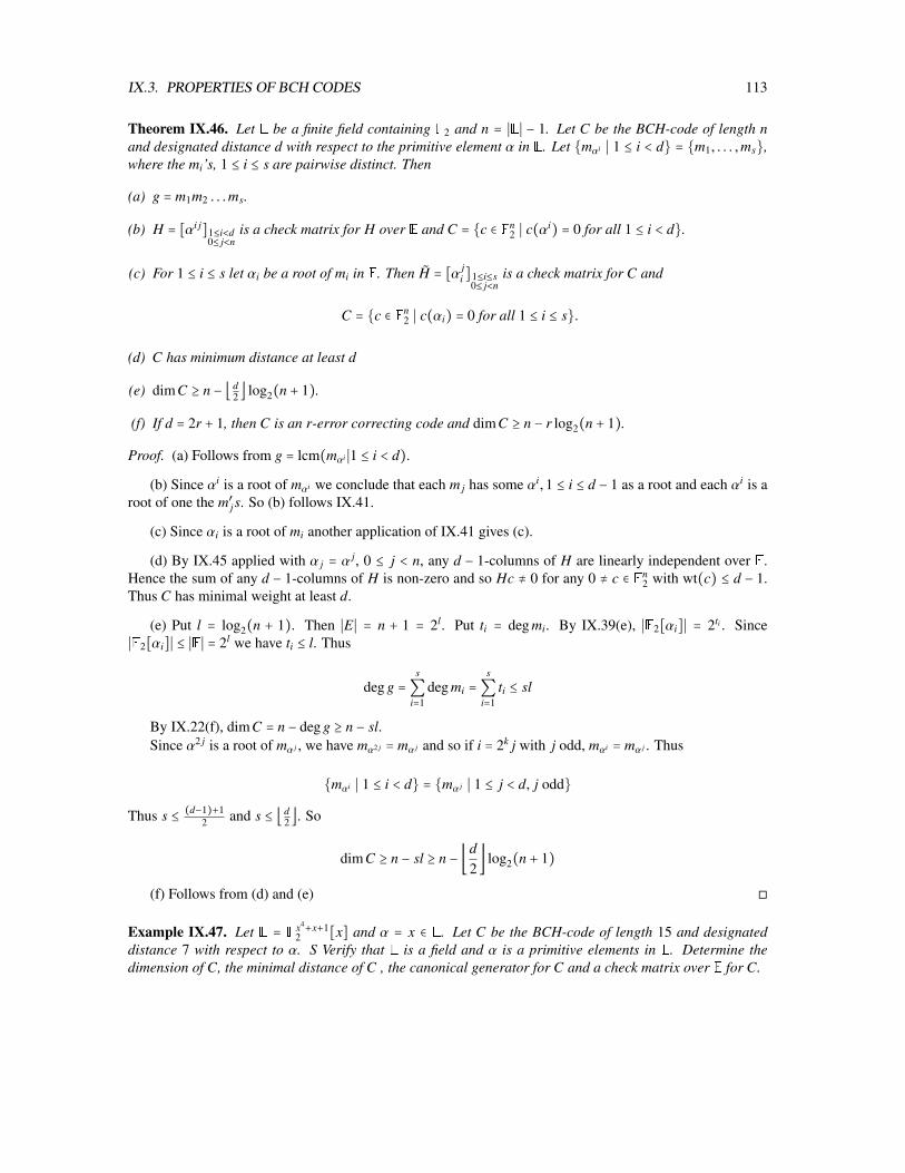
IX.3. PROPERTIES OF BCH CODES 113
Theorem IX.46. Let E be a finite field containing F2 and n = ∣E∣ − 1. Let C be the BCH-code of length nand designated distance d with respect to the primitive element α in E. Let mαi ∣ 1 ≤ i < d = m1, . . . ,ms,where the mi’s, 1 ≤ i ≤ s are pairwise distinct. Then
(a) g = m1m2 . . .ms.
(b) H = [αi j]1≤i<d0≤ j<n
is a check matrix for H over E and C = c ∈ Fn2 ∣ c(αi) = 0 for all 1 ≤ i < d.
(c) For 1 ≤ i ≤ s let αi be a root of mi in E. Then H = [α ji ]1≤i≤s
0≤ j<nis a check matrix for C and
C = c ∈ Fn2 ∣ c(αi) = 0 for all 1 ≤ i ≤ s.
(d) C has minimum distance at least d
(e) dimC ≥ n − ⌊ d2 ⌋ log2(n + 1).
(f) If d = 2r + 1, then C is an r-error correcting code and dimC ≥ n − r log2(n + 1).
Proof. (a) Follows from g = lcm(mαi ∣1 ≤ i < d).
(b) Since αi is a root of mαi we conclude that each m j has some αi,1 ≤ i ≤ d − 1 as a root and each αi is aroot of one the m′
js. So (b) follows IX.41.
(c) Since αi is a root of mi another application of IX.41 gives (c).
(d) By IX.45 applied with α j = α j, 0 ≤ j < n, any d − 1-columns of H are linearly independent over E.Hence the sum of any d − 1-columns of H is non-zero and so Hc ≠ 0 for any 0 ≠ c ∈ Fn
2 with wt(c) ≤ d − 1.Thus C has minimal weight at least d.
(e) Put l = log2(n + 1). Then ∣E∣ = n + 1 = 2l. Put ti = deg mi. By IX.39(e), ∣F2[αi]∣ = 2ti . Since∣F2[αi]∣ ≤ ∣E∣ = 2l we have ti ≤ l. Thus
deg g =s
∑i=1
deg mi =s
∑i=1
ti ≤ sl
By IX.22(f), dimC = n − deg g ≥ n − sl.Since α2 j is a root of mα j , we have mα2 j = mα j and so if i = 2k j with j odd, mαi = mα j . Thus
mαi ∣ 1 ≤ i < d = mα j ∣ 1 ≤ j < d, j odd
Thus s ≤ (d−1)+12 and s ≤ ⌊ d
2 ⌋. So
dimC ≥ n − sl ≥ n − ⌊d2⌋ log2(n + 1)
(f) Follows from (d) and (e)
Example IX.47. Let E = Fx4+x+12 [x] and α = x ∈ E. Let C be the BCH-code of length 15 and designated
distance 7 with respect to α. S Verify that E is a field and α is a primitive elements in E. Determine thedimension of C, the minimal distance of C , the canonical generator for C and a check matrix over E for C.

114 CHAPTER IX. ALGEBRAIC CODING THEORY
To show that E is a field it suffices to show that x4 + x + 1 is irreducible in F2[x]. (see Lemma IX.33).Suppose that x4 + x+ 1 = pq with p,q ∈ F2[x]. Then deg p+ deg q = 4 and we may assume that deg p ≤ 2. Wehave 04 + 0 + 1 = 1 and 14 + 1 + 1 = 1 and so neither 0 nor 1 is a root of x4 + x + 1. Hence neither 0 nor 1 is aroot of p. Thus p is none of x, x+ 1, x2 + 1, x2 + x and x2. To determined whether x2 + x+ 1 divides x4 + x+ 1we use long devision of polynomials:
11111110011
1111111111
1
So the remainder of x4 + x+1 when divide by x2 + x+1 is 1. So p ≠ x2 + x+1. We proved that p is neithera polynomial of degree 1 nor 2. Hence deg p = 0 and x4 + x + 1 is irreducible.
To show that α is a primitive element we compute the powers of α:
α0 = 1 α8 = 1 + α2
α1 = α α9 = α + α3
α2 = α2 α10 = 1 + α + α2
α3 = α3 α11 = α + α2 + α3
α4 = 1 + α α12 = 1 + α + α2 + α3
α5 = α + α2 α13 = 1 + α2 + α3
α6 = α2 + α3 α14 = 1 + α3
α7 = 1 + α + α3 α15 = 1
So α is indeed a primitive elements. To find the canonical generator g we need to determine mαi for1 ≤ i < 7.
α, α2 and α4 are roots of 1 + x + x4 and so mα = mα2 +mα4 .We look at the powers of α3 as strings of length 4
(α3)0 = 1↔ 1000
(α3)1 = α3 ↔ 0001
(α3)2 = α6 ↔ 0011
(α3)3 = α9 ↔ 0101
(α3)4 = α12 ↔ 1111
The first four strings are linearly independent. The sum of all five is zero.So α3 and α6 have minimal polynomial 1 + x + x2 + x3 + x4.
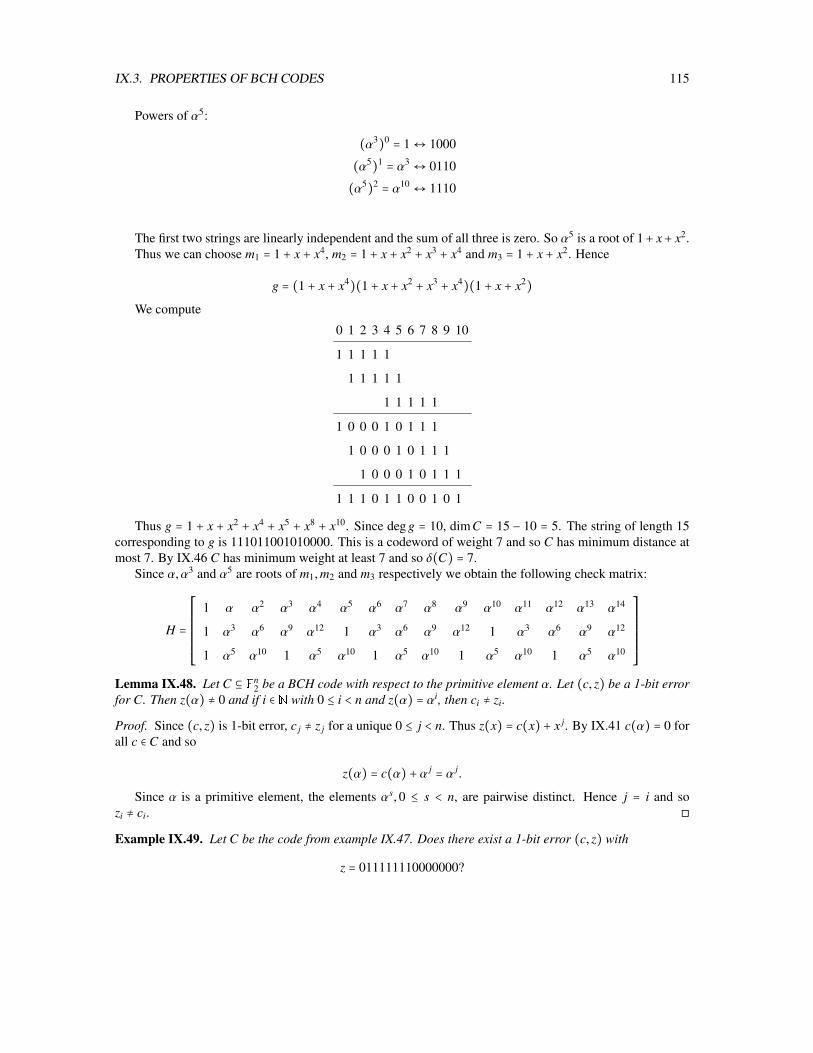
IX.3. PROPERTIES OF BCH CODES 115
Powers of α5:
(α3)0 = 1↔ 1000
(α5)1 = α3 ↔ 0110
(α5)2 = α10 ↔ 1110
The first two strings are linearly independent and the sum of all three is zero. So α5 is a root of 1+ x+ x2.Thus we can choose m1 = 1 + x + x4, m2 = 1 + x + x2 + x3 + x4 and m3 = 1 + x + x2. Hence
g = (1 + x + x4)(1 + x + x2 + x3 + x4)(1 + x + x2)
We compute
0 1 2 3 4 5 6 7 8 9 10
1 1 1 1 1
1 1 1 1 1
1 1 1 1 1
1 0 0 0 1 0 1 1 1
1 0 0 0 1 0 1 1 1
1 0 0 0 1 0 1 1 1
1 1 1 0 1 1 0 0 1 0 1
Thus g = 1 + x + x2 + x4 + x5 + x8 + x10. Since deg g = 10, dimC = 15 − 10 = 5. The string of length 15corresponding to g is 111011001010000. This is a codeword of weight 7 and so C has minimum distance atmost 7. By IX.46 C has minimum weight at least 7 and so δ(C) = 7.
Since α,α3 and α5 are roots of m1,m2 and m3 respectively we obtain the following check matrix:
H =
⎡⎢⎢⎢⎢⎢⎢⎢⎢⎣
1 α α2 α3 α4 α5 α6 α7 α8 α9 α10 α11 α12 α13 α14
1 α3 α6 α9 α12 1 α3 α6 α9 α12 1 α3 α6 α9 α12
1 α5 α10 1 α5 α10 1 α5 α10 1 α5 α10 1 α5 α10
⎤⎥⎥⎥⎥⎥⎥⎥⎥⎦Lemma IX.48. Let C ⊆ Fn
2 be a BCH code with respect to the primitive element α. Let (c, z) be a 1-bit errorfor C. Then z(α) ≠ 0 and if i ∈ N with 0 ≤ i < n and z(α) = αi, then ci ≠ zi.
Proof. Since (c, z) is 1-bit error, c j ≠ z j for a unique 0 ≤ j < n. Thus z(x) = c(x) + x j. By IX.41 c(α) = 0 forall c ∈ C and so
z(α) = c(α) + α j = α j.
Since α is a primitive element, the elements αs,0 ≤ s < n, are pairwise distinct. Hence j = i and sozi ≠ ci.
Example IX.49. Let C be the code from example IX.47. Does there exist a 1-bit error (c, z) with
z = 011111110000000?

116 CHAPTER IX. ALGEBRAIC CODING THEORY
We have z(α) = α + α2 + α3 + α4 + α5 + α6 + α7. We calculate the remainder of this polynomial whendivided by x4 + x + 1.
1111001111111110
10011110011010011
10101010011
1100
Thus z(α) = α3 + α2 = α2(1 + α) = α2α4 = α6. So if (c, z) is a 1-bit error, then the error occurred in bit 7:
c = 0111110100000000
We compute c(α3) and c(α5) to check whether c is in the code:
c(α5) = 0 + α5 + α10 + 1 + α5 + α10 + 0 + α5 = 1 + α5 ≠ 0
So c is not in the code. Thus z cannot be the result of a 1-bit-error.

Chapter X
Cryptography in theory and practice
X.1 Encryption in terms of a channelDefinition X.1. A cryptosystem Ω is quadruple (M,C, (Ek)k∈K, (Dl)l∈K), whereM, C and K are alphabetsand for k ∈ K, Ek ∶M → C and Dk ∶ C →M are functions such that for each k ∈ K there exists k∗ ∈ K withDk∗ Ek = idM.
The elements ofM are called plaintext messages, the elements of C are called ciphertext messages, theelements of K are called keys, each Ek is called an encryption function and each Dl is called an decryptionfunction.
Example X.2. LetM = C = A = A,B,C,D, . . . ,Z,⊔, K = 0,1, . . . ,25 and for k ∈ K, Ek = Dk = ck, whereck is the shift by k-letters defined in Example I.20. Note that D26−k is the inverse of Ek, so this is indeed acryptosystem.
Definition X.3. Let (M,C, (Ek)k∈K, (Dl)l∈K) be a cryptosystem and p and r probabilty distribution onMand K, respectively. Define
u ∶ M ×K × C → [0,1]
(m, k, c) →⎧⎪⎪⎨⎪⎪⎩
pmrk if c = Ek(m)0 if c ≠ Ek(m)
t, q, and s are defined to by the marginal distribution of u onM × C, C and K × C respectively.Define theM × C-matrix Γ by
Γmc = ∑k∈K
Ek(m)=c
rk
Γ is called the encryption channel for the cryptosystem with respect to r.
We interpreted umkc as the probability Prob(m, k, c) that plain text message m was encrypted via the keyk and the cipher text c was obtained.
Lemma X.4. With the notation as in X.3
(a) u is a probability distribution.
117

118 CHAPTER X. CRYPTOGRAPHY IN THEORY AND PRACTICE
(b) p, r and p⊗ r are the marginal distribution of u onM,K andM ×K, respectively.
(c) Γ is a channel associated to the distribution t onM × C.
(d) Ek is 1-1 for all k ∈ K.
(e)qc = ∑
(m,k)∈M×KEk(m)=c
pmrk.
(f) skc = 0 if c /∈ Ek(M) and sk,c = pmrk if c ∈ Ek(M) and m is the unique element ofM with Ek(m) = c.
(g) H(s) = H(p⊗ r) = H(p) + H(r).
(h) H(r∣q) = H(r) + H(p) − H(q).
Proof. Let m ∈M, k ∈ K and c ∈ C.(a) and (b) Clearly umkc ∈ [0,1]. Given m and k, then c∗ = Ek(m) is the only element of C with umkc∗ ≠ 0.
Thus
∑c∈C
umkc = umkc∗ = pmrk.
So p⊗ r is the marginal distribution of u onM×K. Since p⊗ r is a probability distribution, we concludefrom IV.6 that also u is a probablity distribution. Since p and r are the marginal distributions of p⊗ r onMand K, respectively, they are also the marginal distributions of u onM and K, see B.1 in the appendix.
(c) We will first verify that Γ is a channel: Let m ∈M, then
∑c∈C
Γmc =∑c∈C
( ∑k∈K
Ek(m)=c
rk) = ∑k∈K,c∈CEk(m)=c
rk = ∑k∈K
rk = 1
So Γ is indeed a channel.
Since umkc = 0 for c ≠ Ek(m) we have
tmc = ∑k∈K
umkc = ∑k∈K
Ek(m)=c
umkc = ∑k∈K
Ek(m)=c
pmrk = pm ∑k∈K
Ek(m)=c
rk = pmΓmc
Thus t = Diag(p)Γ and so (see Definition V.10(d)) Γ is a channel associated to t.(d) Let k ∈ K and m1,m2 ∈M with Ek(m1) = Ek(m2). By definition of a cryptosystem there exists k∗ ∈ K
with Dk∗ Ek = idM. Thus
m1 = Dk∗(Ek(m1)) = Dk∗(Ek(m2)) = m2
and so Ek is 1-1.(e) Since p and q are the marginal distributions of t, p = qΓ. So using (c),
qc = ∑m∈M
pmΓmc = ∑m∈M
pm( ∑k∈K
Ek(m)=c
rk) = ∑(m,k)∈M×K
Ek(m)=c
pmrk.
(f) Since s is the marginal distribution of u on K × C, skc = ∑m∈M umkc = ∑ m∈MEk(m)=c
pmrk

X.2. PERFECT SECRECY 119
Since Ek is 1-1, there either exists a unique m ∈M with Ek(m) = c or there exists no element m ∈Mwith Ek(m) = c. This gives (f).
(g) Since p and r are independent with respect to p⊗ r, IV.9 gives
H(p⊗ r) = H(p) + H(r)
Consider the function:
π ∶M ×K → K × C, (m, k)→ (k,Ek(m))
Since each Ek is 1-1, also π is 1-1 and so π is a bijection fromM ×K to Imπ. Let k ∈ K and c ∈ C. If(k, c) = π(m, k) for some m ∈M, then (e) shows that
sπ(m,k) = skc = pmrk = (p⊗ r)mk
Since π is a bijection fromM ×K to Imπ, V.17(a) gives
H(p⊗ r) = H(s∣Im π)
Also skc = 0 if (k, c) ∉ Imπ. So
H(s∣Im π) = H(s)
and (g) holds.(h) Using the definition of H(r ∣ q) and (g),
H(r ∣ q) = H(s) − H(q) = H(p) + H(r) − H(q).
Definition X.5. (a) The key equivocation of a cryptosystem with respect to the probability distribution p andr onM and K, respectively, is
H(r∣q)
(b) A cryptosytem is said to have perfect secrecy with respect to the probability distribution r on K if
I(p,q) = 0.
for all probability distributions p onM.Here Γ, r, s and q are as define in X.3.
H(r∣q) measures the amount of information obtained about the keys by observing ciphertext messages.I(p,q) measures the dependency of p and q. I(p,q) = 0 means that p and q are independent. So knowing
the ciphertext does not reveal any information about the plaintext messages.
X.2 Perfect secrecyTheorem X.6. Given a cryptosystem and a probability distribution r onK. Then the following are equivalent:
(a) The cryptosystem has perfect secrecy with respect to the probability distribution r.
(b) p and q are independent for all probability distributions p onM.

120 CHAPTER X. CRYPTOGRAPHY IN THEORY AND PRACTICE
(c) There exists a positive probability distribution p onM such that p and q are independent.
(d) There exists a positive probability distribution p onM such that Γmc = qc for all m ∈M and all c ∈ C,
(e) Each column of Γ is constant, that is there exist a C-tuple (lc)c∈C with Γmc = lc for all m ∈ Γ, c ∈ C.
(f) Γmc = qc for all probability distributions p onM, all m ∈M and all c ∈ C:
Proof. (a)⇐⇒ (b) : By V.19 I(p,q) = 0 if and only if p and q are independent.(b)Ô⇒ (c): Just choose p to be the equal probability distribution onM.(c) Ô⇒ (d): Since p and q independent we have tmc = pmqc for all m ∈ M and c ∈ C. Since Γ is a
channel associated to t, tmc = pmΓmc. Thus pmΓmc = pmqc for all m ∈M and all c ∈ C. Since p is positivepm ≠ 0 and so Γmc = qc.
(d)Ô⇒ (e): All entries in column c of Γ are equal to qc.(e) Ô⇒ (f): Let c ∈ C. Since column c of Γ is constant there exists lc ∈ [0,1] with Γmc = lc for all
m ∈M. Let p be any probability distribution onM. Then
qc = ∑m∈M
pmΓmc = ∑m∈M
pmlc = ( ∑m∈M
pm) lc = 1lc = lc
and so (f) holds.(f) Ô⇒ (b): Let p be a probability distribution onM. Then tmc = pmΓmc = pmqc and so p and q are
independent with respect to t. Thus (b) holds.
Corollary X.7. If a cyrptosystem has perfect secrecy (with respect to some probability distribution on K),then the numbers of keys is greater or equal to the number of plaintext messages.
Proof. Fix c ∈ C with qc ≠ 0. Then by X.6 Γmc = qc > 0 for all m ∈M. By X.4
∑k∈K
Ek(m)=c
rk = Γmc > 0
and so for all m ∈M there exists km ∈ K with Ekm(m) = c. Suppose k ∶= km = km for some m, m ∈M. ThenEk(m) = c = Ek(m) and since Ek is 1-1, m = m. So the map m→ km is 1-1 and thus ∣M∣ ≤ ∣K∣.
X.3 The one-time padDefinition X.8. Let F be a finite field (or let (F,+) be finite group) and let n ∈ Z+. For k ∈ Fn define
Ek = Dk ∶ Fn → Fn,m→ m + k
Then Ω(Fn) = (Fn,Fn, (Ek)k∈Fn , (Dk)k∈Fn) is called the one-time pad determined by Fn.
Lemma X.9 (One-Time Pad). Any one-time pad is a cryptosystem and has perfect secrecy with respectrespect to the equal-probability distribution r on the set of keys.
Proof. Given a one-time pad Ω(Fn). Since (m + k) + (−k) = m + (k + (−k)) = m + 0 = m, D−k Ek = idFn .Thus the one-time pad is a cryptosystem.
Put e = 1∣Fn∣ . Then rk = e for all k ∈ K.
Let m ∈M and c ∈ C. By definition Γ and Ek:
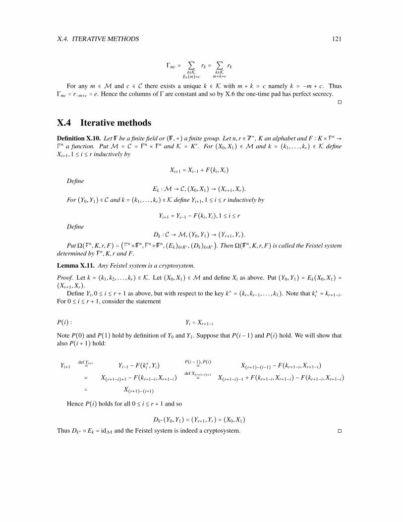
X.4. ITERATIVE METHODS 121
Γmc = ∑k∈K
Ek(m)=c
rk = ∑k∈K
m+k=c
rk
For any m ∈ M and c ∈ C there exists a unique k ∈ K with m + k = c namely k = −m + c. ThusΓmc = r−m+c = e. Hence the columns of Γ are constant and so by X.6 the one-time pad has perfect secrecy.
X.4 Iterative methodsDefinition X.10. Let F be a finite field or (F,+) a finite group. Let n, r ∈ Z+, K an alphabet and F ∶ K×Fn →F
n a function. Put M = C = Fn × Fn and K = Kr. For (X0,X1) ∈ M and k = (k1, . . . , kr) ∈ K define
Xi+1,1 ≤ i ≤ r inductively by
Xi+1 = Xi−1 + F(ki,Xi)Define
Ek ∶M→ C, (X0,X1)→ (Xr+1,Xr).For (Y0,Y1) ∈ C and k = (k1, . . . , kr) ∈ K define Yi+1,1 ≤ i ≤ r inductively by
Yi+1 = Yi−1 − F(ki,Yi),1 ≤ i ≤ r
DefineDk ∶ C →M, (Y0,Y1)→ (Yr+1,Yr).
Put Ω(Fn,K, r,F) = (Fn×Fn,Fn×Fn, (Ek)k∈Kr , (Dk)k∈Kr). Then Ω(Fn,K, r,F) is called the Feistel systemdetermined by Fn,K, r and F.
Lemma X.11. Any Feistel system is a cryptosystem.
Proof. Let k = (k1, k2, . . . , kr) ∈ K. Let (X0,X1) ∈M and define Xi as above. Put (Y0,Y1) = Ek(X0,X1) =(Xr+1,Xr).
Define Yi,0 ≤ i ≤ r + 1 as above, but with respect to the key k∗ = (kr, kr−1, . . . , k1). Note that k∗i = kr+1−i.For 0 ≤ i ≤ r + 1, consider the statement
P(i) ∶ Yi = Xr+1−i
Note P(0) and P(1) hold by definition of Y0 and Y1. Suppose that P(i− 1) and P(i) hold. We will show thatalso P(i + 1) hold:
Yi+1def Yi+1= Yi−1 − F(k∗i ,Yi)
P(i − 1), P(i)= X(r+1)−(i−1) − F(kr+1−i,Xr+1−i)
= X(r+1−i)+1 − F(kr+1−i,Xr+1−i)def X(r+1−i)+1= X(r+1−i)−1 + F(kr+1−i,Xr+1−i) − F(kr+1−i,Xr+1−i)
= X(r+1)−(i+1)
Hence P(i) holds for all 0 ≤ i ≤ r + 1 and so
Dk∗(Y0,Y1) = (Yr+1,Yr) = (X0,X1)Thus Dk∗ Ek = idM and the Feistel system is indeed a cryptosystem.
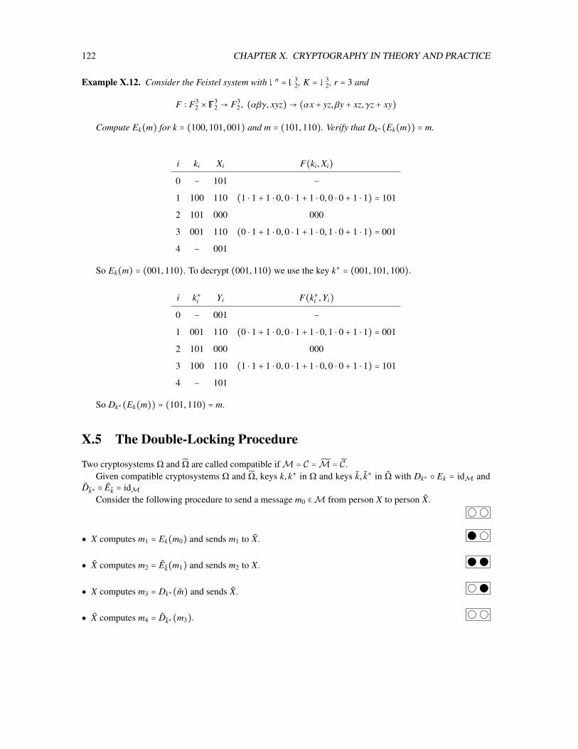
122 CHAPTER X. CRYPTOGRAPHY IN THEORY AND PRACTICE
Example X.12. Consider the Feistel system with Fn = F32, K = F3
2, r = 3 and
F ∶ F32 × F3
2 → F32 , (αβγ, xyz)→ (αx + yz, βy + xz, γz + xy)
Compute Ek(m) for k = (100,101,001) and m = (101,110). Verify that Dk∗(Ek(m)) = m.
i ki Xi F(ki,Xi)
0 − 101 −
1 100 110 (1 ⋅ 1 + 1 ⋅ 0,0 ⋅ 1 + 1 ⋅ 0,0 ⋅ 0 + 1 ⋅ 1) = 101
2 101 000 000
3 001 110 (0 ⋅ 1 + 1 ⋅ 0,0 ⋅ 1 + 1 ⋅ 0,1 ⋅ 0 + 1 ⋅ 1) = 001
4 − 001
So Ek(m) = (001,110). To decrypt (001,110) we use the key k∗ = (001,101,100).
i k∗i Yi F(k∗i ,Yi)
0 − 001 −
1 001 110 (0 ⋅ 1 + 1 ⋅ 0,0 ⋅ 1 + 1 ⋅ 0,1 ⋅ 0 + 1 ⋅ 1) = 001
2 101 000 000
3 100 110 (1 ⋅ 1 + 1 ⋅ 0,0 ⋅ 1 + 1 ⋅ 0,0 ⋅ 0 + 1 ⋅ 1) = 101
4 − 101
So Dk∗(Ek(m)) = (101,110) = m.
X.5 The Double-Locking Procedure
Two cryptosystems Ω and Ω are called compatible ifM = C = M = C.Given compatible cryptosystems Ω and Ω, keys k, k∗ in Ω and keys k, k∗ in Ω with Dk∗ Ek = idM and
Dk∗ Ek = idMConsider the following procedure to send a message m0 ∈M from person X to person X.
X computes m1 = Ek(m0) and sends m1 to X.
X computes m2 = Ek(m1) and sends m2 to X.
X computes m3 = Dk∗(m) and sends X.
X computes m4 = Dk∗(m3).

X.5. THE DOUBLE-LOCKING PROCEDURE 123
m0EkÐÐÐÐ→ m1
EkÐÐÐÐ→ m2Dk∗ÐÐÐÐÐ→ m3
Dk∗ÐÐÐÐÐ→ m4
Is m4 = m0?Consider the following exampleM = C = 1,2,3,
Ek = Dk∗ ∶1 2 3
1 3 2Ek = Dk∗ ∶
1 2 3
2 1 3
and m0 = 1
1EkÐÐÐÐ→ 1
EkÐÐÐÐ→ 2Dk∗ÐÐÐÐÐ→ 3
Dk∗ÐÐÐÐÐ→ 3
So m4 ≠ m0.In general
m4 = (Dk∗ Dk∗ Ek Ek)(m0)If Dk∗ commutes with Ek, that is Dk∗ Ek = Ek Dk∗ then
Dk∗ Dk∗ Ek Ek = (Dk∗ Ek) (Dk∗ Ek) = idM idM = idM
and procedure works.
Since addition in finite field is commutative, one-time pads provide examples where Dk∗ commutes withEk.
Example X.13. Suppose Ω and Ω both are the one-time pad determined by F42. Given the following public
information:
m0EkÐÐÐÐ→ 1101
EkÐÐÐÐ→ 0110Dk∗ÐÐÐÐÐ→ 1100
Dk∗ÐÐÐÐÐ→ m4
What is m0?
Since 0110 + k∗ = 1100 and so k∗ = 1100− 0110 = 1010. So m0 = D∗
k (m1) = 1101+ 1010 = 0111.
So one-time pads should not be used for the double-locking procedure.
Lemma X.14. Let Ω and Ω be compatible cryptosystem. Let β be an encryption function in Ω and let γ andγ′ be decryption functions in Ω which commute with β, that is
γ β = β γ, and γ′ β = β γ′
Let m1 ∈M and put m2 = β(m1). Then
γ(m2) = γ′(m2) Ô⇒ γ(m1) = γ′(m2)Proof.
β(γ(m1)) = (β γ)(m1) = (γ β)(m1) = γ(β(m1)) = γ(m2)
By symmetry, β(γ′(m1)) = γ′(m2). So if γ(m2) = γ′(m2) we conclude that
β(γ(m1)) = β(γ′(m1))Since encryption functions are 1-1, we get γ(m1) = γ′(m1).
The lemma shows that the double locking procedure is very vulnerable: Anybody who intercepts themessage m1, m2 and m3 and is able to find a decryption function Dl in Ω with Dl(m2) = m3 can compute m0,namely m0 = Dl(m1).

124 CHAPTER X. CRYPTOGRAPHY IN THEORY AND PRACTICE

Chapter XI
The RSA cryptosystem
XI.1 Public-key cryptosytemsDefinition XI.1. A public-key cryptosystem is pair (Ω, ξ) where Ω is a cryptosystem and ξ is a function
ξ ∶ A→ K ×K, a→ (ka, k∗a )
such that for all a ∈ ADk∗a Eka = idM
ka is called a public key and k∗a a private key.
In public key cryptography, all the ingredients except the privat key are know to the public. Anybody thencan encrypt a message using the public key k and the publicly known function Ek. But only somebody whoknows the private key k∗ is able to decrypt the encrypted message using the function Dl. This can only workif it is virtually impossible to determine k∗ from k. In particular, A has to be really large, since otherwise onecan just compute all the possible pairs (k, k∗) using the publicly known function ξ.
In this sections we will describe a public-key cryptosystem discovered by Rivest, Shamir and Adlemanin 1977 known as the RSA cryptosystem. But we first need to prove a couple of lemmata about the ring ofintegers.
XI.2 The Euclidean AlgorithimLemma XI.2. Let a,b,q and r be integers with a = qb + r. Then gcd(a,b) = gcd(b, r).
Proof. Let d = gcd(a,b) and e = gcd(b, r). Then d divides a and b and so also r = a − qb. Hence d is acommon divisor of b and r. Thus d ≤ e.
Similarly, e divides b and r and so also a = qb + r. Thus e is a common divisor of a nd b and so e ≤ d.Hence e = d.
Theorem XI.3 (Euclidean Algorithm). Let a and b be integers and let E−1 and E0 be the equations
E−1 ∶ a = 1a + 0b
E0 ∶ b = 0a + 1b,
125

126 CHAPTER XI. THE RSA CRYPTOSYSTEM
and suppose inductively we defined equation Ek,−1 ≤ k ≤ i of the form
Ek ∶ rk = xka + ykb .
If ri ≠ 0, let Ei+1 be equation obtained by subtracting qi+1 times equation Ei from Ei−1 where qi+1 is the integerquotient of ri−1 when divided by ri (so qi+1 = ⌊ ri−1
ri⌋). Let m ∈ N be minimal with rm = 0 and put d = rm−1,
x = xm−1 and y = ym−1. Then
(a) gcd(a,b) = ∣d∣
(b) x, y ∈ Z and d = xa + yb.
Proof. Observe that ri+1 = ri−1−qi+1ri, xi+1 = xi−1−qi+1xi and yi+1 = yi−1−qi+1xi. So inductively ri+1, xi+1, yi+1are integers and ri+1 is the remainder of ri−1 when divided by ri. So ri+1 < ∣ri∣ and the algortithm will terminatein finitely many steps.
From ri−1 = qi+1ri + ri+1 and XI.2 we have gcd(ri−1, ri) = gcd(ri, ri+1) and so
gcd(a,b) = gcd(r−1, r0) = gcd(r0, r1) = . . . = gcd(rm−1, rm) = gcd(d,0) = ∣d∣
So (a) holds. Since each xi and yi are integers, x and y are integers. d = xa + yb is just the equationEm−1.
Example XI.4. Let a = 1492 and b = 1066. Then
1492 = 1 ⋅1492 + 0 ⋅ 1066
1066 = 0 ⋅1492 + 1 ⋅ 1066 q1 = 1
426 = 1 ⋅1492 − 1 ⋅ 1066 q2 = 2
214 = −2 ⋅1492 + 3 ⋅ 1066 q3 = 1
212 = 3 ⋅1492 − 4 ⋅ 1066 q4 = 1
2 = −5 ⋅1492 + 7 ⋅ 1066 q5 = 106
0
So gcd(1492,1066) = 2 and 2 = −5 ⋅ 1492 + 7 ⋅ 1066.
Definition XI.5. Let n ∈ Z+ and a,b ∈ Z. Then
Zn = a ∈ Z ∣ 0 ≤ a < n,
Z∗n = a ∈ Zn ∣ gcd(a,n) = 1,
andφ(n) = ∣Z∗n ∣.
If a ∈ Z, then [a]n denotes the remainder of a when divided by n. We will sometimes also use the notationa for [a]n.
The relation ‘ ≡ (mod n)’ on Z is defined by
a ≡ b (mod n) ⇐⇒ n ∣ b − a

XI.2. THE EUCLIDEAN ALGORITHIM 127
Lemma XI.6. Let a,b,a′,b′,n ∈ Z with n > 0. If
a ≡ a′ (mod n) and b ≡ b′ (mod n)then
ab ≡ a′b′ (mod n)
Proof. Since a ≡ a′ there exists k ∈ Z with a′ − a = kn. So a′ = a + kn. By symmetry, b′ = b + ln for somel ∈ Z. Thus
a′b′ − ab = (a + kn)(b + ln) − ab = (al + kb + kln)n
So n divides a′b′ − ab the lemma holds.
Lemma XI.7. Let n ∈ Z+ and d ∈ Z∗n . Then there exists e ∈ Z∗n with de ≡ 1 (mod n).
Proof. By the Euclidean algorithm there exist r, s ∈ Z with
1 = gcd(d,n) = rd + sn.
Hence rd ≡ 1 (mod n). Put e = [r]n. Then 0 ≤ e < n and so e ∈ Zn. Note that e ≡ r (mod n) and so byXI.6 ed ≡ rd ≡ 1 (mod n).
In particular, n ∣ ed − 1 and any divisor of n and e will divide 1. Thus gcd(n, e) = 1 and e ∈ Z∗n .
Lemma XI.8. Let n,m ∈ Z with n > 0. Then gcd(n,m) = gcd(n, [m]n).
Proof. Observe that m = qn + [m]n for some q ∈ Z and so the lemma follows from XI.2.
Lemma XI.9. Let n ∈ Z+, a,b ∈ Zn and d ∈ Z∗n .
(a) If a ≡ b (mod n), then a = b.
(b) If [ad]n = [bd]n, then a = b.
Proof. (a) Since a ≡ b (mod n), n ∣ a − b. Since a,b ∈ Z∗n we have ∣a − b∣ < n. Thus a − b = 0 and a = b.(b) By XI.7 there exists e ∈ Z∗n with de ≡ 1 (mod n). Note that ad ≡ bd (mod n) and so ead ≡ ebd
(mod n) and dea ≡ deb (mod n). Thus a ≡ b (mod n) and so by (a) a = b.
Lemma XI.10. Let n,m ∈ Z+ with gcd(n,m) = 1. Then φ(nm) = φ(n)φ(m).
Proof. Consider the map
α ∶ Znm → Zn ×Zm,a→ ([a]n, [a]m)We claim that α is 1 − 1 and onto. Let a,b ∈ Znm with [a]n = [b]n and [a]m = [b]m. Then n and m divideda − b and since gcd(n,m) = 1, nm ∣ a − b. Hence a = b by XI.9(a). So α is 1-1. Since ∣Znm∣ = nm = ∣Zn ×Zm∣,α is also onto.
Since gcd(n,m) = 1, gcd(a,nm) = gcd(a,n)gcd(a,m). Hence gcd(a,nm) = 1 if and only if gcd(a,n) = 1and gcd(a,m) is 1. By XI.8 this holds if and only if gcd([a]n,n) = 1 and gcd([a]m,=)1. We proved thata ∈ Z∗nm if and only if ([a]n, [b]m) ∈ Z∗n ×Z∗m. Thus α induces a bijection
α∗ ∶ Z∗nm → Z∗n ×Z∗m, a→ ([a]n, [a]m).
Soφ(nm) = ∣Z∗nm∣ = ∣Z∗n ×Z∗m∣ = φ(n)φ(m).

128 CHAPTER XI. THE RSA CRYPTOSYSTEM
Corollary XI.11. Let p and q be distinct primes. The φ(p) = p−1 and φ(pq) = (p−1)(q−1) = pq+1−(p+q).
Proof. Z∗p = 1,2, . . . , p − 1 and so φ(p) = p − 1. By XI.10 φ(pq) = φ(p)φ(q) = (p − 1)(q − 1).
Lemma XI.12. Let a ∈ Z∗n . Then aφ(n) ≡ 1 (mod n).
Proof. For d ∈ Z put d = [d]n. Let b ∈ Z∗n . Note that gcd(ab,n) = 1 and so by XI.8, also gcd(ab,n) = 1. Thusab ∈ Z∗n and we obtain an map
α ∶ Z∗n → Z∗n ,b→ ab.
By XI.9, α is 1 − 1 and so also onto.It follows that
∏b∈Z∗n
b = ∏b∈Z∗n
ab.
Since ab ≡ ab (mod n) we conclude from XI.6 that
∏b∈Z∗n
b ≡ ∏b∈Z∗n
ab (mod n).
Put e =∏b∈Z∗n b. Then the above equation reads
1e = e ≡ aφ(n)e (mod n).Thus by XI.9
aφ(n) ≡ 1 (mod n).
XI.3 Definition of the RSA public-key cryptosystemDefinition XI.13. LetM be any alphabet of plain text messages and c a positive integer. Put
C = n ∈ Z+ ∣ n ≤ c, N = n ∈ C ∣ φ(n) ≥ ∣M∣, and K = (n,d) ∣ n ∈ N,d ∈ Z∗φ(n)
For n ∈ N let αn ∶M→ Z∗n be a code and βn ∶ Zn →M a function with βn(αn(m)) = m for all m ∈M.
Given a key (n,d) ∈ K. For m ∈M define
En,d(m) = [αn(m)d]n
and for z ∈ C define
Dn,d(z) = βn ([zd]n)
Let π be a set of primes with ∣M∣ ≤ (p − 1)2 ≤ c for all p ∈ π. Put
A = (p,q,d, e) ∣ p,q ∈ π, p ≠ q, d, e ∈ Z∗φ(pq), de ≡ 1(mod φ(pq))Define
ξ ∶ A→ K ×K, (p,q,d, e)→ ((pq,d), (pq, e))
Then (M,C, (En,d)(n,d)∈K, (Dn,d)(n,d)∈K, ξ) is called an RSA public-key cryptosystem.
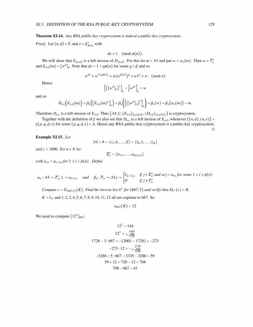
XI.3. DEFINITION OF THE RSA PUBLIC-KEY CRYPTOSYSTEM 129
Theorem XI.14. Any RSA public-key cryptosystem is indeed a public-key cryptosystem.
Proof. Let (n,d) ∈ K and e ∈ Z∗φ(n) with
de ≡ 1 (mod φ(n)).
We will show that E(n,d) is a left inverse of D(n,d). For this let m ∈M and put w = αn(m). Then w ∈ Z∗nand En,d(m) = [wd]n. Note that de = 1 + qφ(n) for some q ∈ Z and so
wde ≡ w1+qφ(n) ≡ w(wφ(n))q ≡ w1q ≡ w (mod n)
Hence[([wd]n)
e]n= [wde]
n= w
and so
Dn,e(En,d(m)) = βn([En,d(m)e]n) = βn([([wd]n)
e]n) = βn(w) = βn(αn(m)) = m.
Therefore Dn,e is a left-inverse of En,d. Thus (M,C, (En,d)(n,d)∈K, (Dn,d)(n,d)∈K) is cryptosystem.Together with the definition of ξ we also see that Dn,e is a left inverse of En,d, whenever ((n,d), (n, e)) =
ξ(p,q,d, e) for some (p,q,d, e) ∈ A. Hence any RSA public-key cryptosystem is a public-key cryptosystem.
Example XI.15. LetM = A = ⊔,A, . . . ,Z = l0, l1 . . . , l26
and c = 1000. For n ∈ N letZ∗n = a1,n, . . . ,aφ(n),n
with ai,n < ai+1,n for 1 ≤ i < φ(n) . Define
αn ∶M→ Z∗n , li → ai+1,n and βn ∶ Zn →M j→
⎧⎪⎪⎨⎪⎪⎩
l[i−1]27 if j ∈ Z∗n and so j = an,i for some 1 ≤ i ≤ φ(n)0 if j ∉ Z∗n
Compute c = E(667,5)(K). Find the inverse key k∗ for (667,5) and verify that Dk∗(c) = K.
K = l11 and 1,2,3,4,5,6,7,8,9,10,11,12 all are coprime to 667. So
α667(K) = 12
We need to compute [125]667:
122 = 144
123 = 1440+ 288
1728
1728 − 3 ⋅ 667 = −(2001 − 1728) = −273
−273 ⋅ 12 = − 2730+ 546
3286
−3286 + 5 ⋅ 667 = 3335 − 3286 = 5959 ∗ 12 = 720 − 12 = 708
708 − 667 = 41

130 CHAPTER XI. THE RSA CRYPTOSYSTEM
Hence E667,5(K) = 41.To compute e we need to factorize 29. None of 3,5,11 divides 667, 667 − 7 = 660, 667 + 13 = 680,
667 − 17 = 650, 667 + 23 = 690. So 667 = 23 ⋅ 29. Thus φ(667) = 667 − (23 + 29) + 1 = 668 − 52 = 616.
1 = 616 − 123 ⋅ 5
So e = 616 − 123 = 493. Since 41493 ≡ 12 (mod 667), we get D667,493(41) = β667(12) = l11 = K.

Appendix A
Rings and Field
A.1 Basic Properties of Rings and FieldsDefinition A.1. A ring is a triple (R,+, ⋅) such that
(i) R is a set;
(ii) + is a function (called ring addition), R × R is a subset of the domain of + and for (a,b) ∈ R × R, a + bdenotes the image of (a,b) under +;
(iii) ⋅ is a function (called ring multiplication), R×R is a subset of the domain of ⋅ and for (a,b) ∈ R×R, a ⋅b(and also ab) denotes the image of (a,b) under ⋅;
and such that the following eight axioms hold:
(Ax 1) a + b ∈ R for all a,b ∈ R; [closure for addition]
(Ax 2) a + (b + c) = (a + b) + c for all a,b, c ∈ R; [associative addition]
(Ax 3) a + b = b + a for all a,b ∈ R. [commutative addition]
(Ax 4) there exists an element in R, denoted by 0R and called ‘zero R’, [additive identity]
such that a + 0R = a = 0R + a for all a ∈ R;
(Ax 5) for each a ∈ R there exists an element in R, denoted by −a [additive inverses]
and called ‘negative a’, such that a + (−a) = 0R;
(Ax 6) ab ∈ R for all a,b ∈ R; [closure for multiplication]
(Ax 7) a(bc) = (ab)c for all a,b, c ∈ R; [associative multiplication]
(Ax 8) a(b + c) = ab + ac and (a + b)c = ac + bc for all a,b, c ∈ R. [distributive laws]
Definition A.2. A ring (R,+, ⋅) is called commutative if
(Ax 9) ab = ba for all a,b ∈ R. [commutative multiplication]
Definition A.3. An element 1R in a ring (R,+, ⋅) is called an (multiplicative) identity if
131

132 APPENDIX A. RINGS AND FIELD
(Ax 10) 1R ⋅ a = a = a ⋅ 1R for all a ∈ R. [multiplicative identity]
Definition A.4. A field is a commutative ring (F,+, ⋅) with identity 1F ≠ 0F such that
(Ax 11) for each a ∈ R with a ≠ 0F there exists an element in R, denoted by a−1 [multiplicative inverses]
and called ‘ a inverse ’, such that a ⋅ a−1 = 1R = a−1 ⋅ a;
If (R,+, ⋅) is a ring, we will often just say that R is a ring, assuming that there is no confusion about theunderlying addition and multiplication. Also we will usually write 0 for 0R and 1 for 1R.
With respect to the usual addition and multiplication:The real number and the rational numbers are fields. The integers are a commutative ring but not a field.
F2 is a field.
Lemma A.5. Let R be ring and a,b ∈ R. Define a − b = a + (−b).
(a) a + 0 = a.
(b) (b + a) + (−a) = b.
(c) Let d ∈ R. Then a = b if and only if d + a = d + b if and only if a + d = b + d
(d) x = b − a is the unique element in R with x + a = b.
(e) x = −a is the unique element in R with x + a = 0.
(f) 0a = 0 = a0.
(g) (−b)a = −(ba).
(h) −(−a) = a
(i) −(a + b) = (−a) + (−b).
(j) −(a − b) = b − a.
(k) If R has an identity, (−1)a = −a.
Proof. (a) a + 0 = 0 + a = a.(b) (b + a) + (−a) = b + (a + (−a)) = b + 0 = b.(c) If a = b, then clearly d + a = d + b. If d + a = d + b, then since d + a = a + d and d + b = b + d, we have
a + d = b + d.Suppose that a+d = b+d. Adding (−d) to both sides of the equation gives (a+d)+(−d) = (b+d)+(−d)
and so by (b), a = b.(d) We have x + a = b if and only if (x + a) + (−a) = b + (−a). bBy (b) and the definition of b − a this
holds if and only if x = b − a.(e) Since −a = 0 + (−a) = 0 − a, this follows from (d) applied with b = 0.(f) We have 0+ 0a = 0a = (0+ 0)a = 0a+ 0a and so by (c), 0 = 0a. A similar argument shows that a0 = 0.(g) ba + (−b)a = (b + (−b))a = 0a = 0 and so −(ba) = (−b)a by (e).(h) By 0 = a + (−a) = (−a) + a and so by (e), a = −(−a).(i) (a + b) + ((−a) + (−b)) = ((a + b) + (−a)) + (−b) = ((b + a) + (−a)) + (−b) = b + (−b) = 0 and so
(−a) + (−b) = −(a + b) by (e).
(h) −(a − b) = −(a + (−b)) (i)= −a + (−(−b)) (h)= −a + b = b + (−a) = b − a.(k) By (g) −a = −(1a) = (−1)a.

A.2. POLYNOMIALS 133
A.2 PolynomialsDefinition A.6. Let R be ring. Then R[x] is the set of N-tuples (ai)i∈N with coefficients in R such that thereexists n ∈ N with ai = 0 for all i > n. We denote such an N-tuple by
a0 + a1x + . . . + anxn.
Let f = ∑ni=0 aixi and g = ∑m
i=0 bixi be elements of R[x] define
f + g =l
∑i=0
(ai + bi)xi,
where l = max(n,m), ai = 0 for i > n and bi = 0 for i > m; and
f g =n+m
∑k=0
(k
∑i=0
aibk−i) xi
Define deg f = maxi ∣ ai ≠ 0 with deg f = −∞ if f = 0.
Lemma A.7. Let R be a ring. Then R[x] is a ring. If R is commutative, so is R[x].
Proof. Readily verified.
Lemma A.8. Let F be a field and f ,g ∈ F[x]. Then
(a) deg( f + g) ≤ max(deg f ,deg g).
(b) deg f g = deg f + deg g.
(c) If f ≠ 0, then deg g ≤ deg f g.
Proof. Readily verified.
Lemma A.9. Let F be a field and h ∈ F[x] with h ≠ 0.
(a) (Fh[x],⊕,⊙) is a commutative ring with identity.
(b) (F[x],⊕,⊙) fulfills Axioms (1)-(9) of a commutative ring, except for Axiom (4) (that is ⊕ has not additiveidentity).
Proof. Let e, f ,g ∈ F[x]. Recall that f denotes the remainder of f when divided by h. By definition of ⊕ and⊙:
1. f ⊕ g = f + g and f ⊙ g = f g.
By IX.8(a)
2. f = f for all f ∈ Fh[x].
By IX.11
3. f ⊕ g = f ⊕ g = f ⊕ g = f + g and f ⊙ g = f ⊙ g = f ⊙ g = f g.

134 APPENDIX A. RINGS AND FIELD
We now will verify all the conditions on a commutative ring (see A.1) Since
f ⊕ g = f + g = g + f = g⊕ f ,
condition (i) holds.We have
e⊕ ( f ⊕ g) = e⊕ f + g = e + ( f + g)) = (e + f ) + g
and
(e⊕ f )⊕ g = e + f ⊕ g = (e + f ) + g.
Thus condition (ii) holds.We have 0⊕ f = 0 + f = f and so for f ∈ Fh[x], 0⊕ f = f . Hence condition (iii) holds.
f ⊕ − f = f + (− f ) = 0 = 0
and condition (iv) is proved.Since
e⊙ ( f ⊙ g) = e⊙ f g = e( f g) = (e f )g
and
(e⊙ f )⊙ g = e f ⊙ g = (e f )g
condition (v) is verified. From
e⊙ ( f ⊕ g) = e⊙ f + g = e( f + g) = e f + eg
and
(e⊙ f )⊕ (e⊙ g) = e f ⊕ eg = e f + eg
we conclude that condition (vi) holds.. A similar argument (or using that ⊙ is commutative) gives condition(vii).
We have
1⊙ f = 1 f = f
and so 1⊙ f = f for all f ∈ Fh[x]. Thus condition (viii) is verified.Finally
f ⊙ g = f g = g f = g⊙ f
and condition (ix) holds.
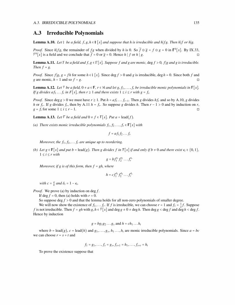
A.3. IRREDUCIBLE POLYNOMIALS 135
A.3 Irreducible PolynomialsLemma A.10. Let F be a field, f ,g,h ∈ F[x] and suppose that h is irreducible and h∣ f g. Then h∣ f or h∣g.
Proof. Since h∣ f g, the remainder of f g when divided by h is 0. So f ⊙ g = f ⊙ g = 0 in Fh[x]. By IX.33,F
h[x] is a field and we conclude that f = 0 or g = 0. Hence h ∣ f or h ∣ g.
Lemma A.11. Let F be a field and f ,g ∈ F[x]. Suppose f and g are monic, deg f > 0, f ∣g and g is irreducible.Then f = g.
Proof. Since f ∣g, g = f h for some h ∈ F[x]. Since deg f > 0 and g is irreducible, deg h = 0. Since both f andg are monic, h = 1 and so f = g.
Lemma A.12. Let F be a field, 0 ≠ a ∈ F, r ∈ N and let g, f1, . . . , fr be irreducible monic polynomials in F[x].If g divides a f1 . . . fr in F[x], then r ≥ 1 and there exists 1 ≤ i ≤ r with g = fi.
Proof. Since deg g > 0 we must have r ≥ 1. Put h = a f1 . . . fr−1. Then g divides h fr and so by A.10, g dividesh or fr. If g divides fr, then by A.11 h = fr. So suppose g divides h. Then r − 1 > 0 and by induction on r,g = fi for some 1 ≤ i ≤ r − 1.
Lemma A.13. Let F be a field and 0 ≠ f ∈ F[x]. Put a = lead( f ).
(a) There exists monic irreducible polynomials f1, f2 . . . , fr ∈ F[x] with
f = a f1 f2 . . . fr
Moreover, the f1, f2, . . . fr are unique up to reordering.
(b) Let g ∈ F[x] and put b = lead(g). Then g divides f in F[x] if and only if b ≠ 0 and there exist εi ∈ 0,1,1 ≤ i ≤ r with
g = b f ε11 f ε2
2 . . . f εrr
Moreover, if g is of this form, then f = gh, where
h = c f δ11 f δ2
2 . . . f δrr
with c = ab and δi = 1 − εi.
Proof. We prove (a) by induction on deg f .If deg f = 0, then (a) holds with r = 0.So suppose deg f > 0 and that the lemma holds for all non-zero polynomials of smaller degree.We will now show the existence of f1, . . . fr. If f is irreducible, we can choose r = 1 and f1 = 1
a f . Supposef is not irreducible. Then f = gh with g,h ∈ F[x] and deg g ≠ 0 ≠ deg h. Then deg g < deg f and deg h < deg f .Hence by induction
g = bg1g2 . . .gs and h = ch1 . . .ht
where b = lead(g), c = lead(h) and g1, . . . ,gs, h1 . . . ,ht are monic irreducible polynomials. Since a = bcwe can choose r = s + t and
f1 = g1, . . . , fs = gs, fs+1 = h1, . . . , fs+t = ht
To prove the existence suppose that

136 APPENDIX A. RINGS AND FIELD
f = a f1 . . . fr = ag1 . . .gs
for some monic irreducible polynomials f1, . . . , fr,g1, . . .gs.Then f1∣ f = ag1 . . .gs and so A.12 show that f1 = gi for some 1 ≤ i ≤ r. Reordering the g′i s we may
assume that f1 = g1. Hence also
a f2 . . . fr = ag2 . . .gs
The induction assumptions implies that r = s and after reordering f2 = g2, . . . , fr = gr.So the fi’s are unique up to reordering.(b) If g and h are of the given form then gh = f and so g is a divisor of f .Suppose now that g divides f . Then f = gh for some h ∈ F[x]. If deg g = 0, then (a) holds with εi = 0 for
all 1 ≤ i ≤ r. So suppose deg g = 0. By (a) we can write g = tg where t is an irreducible monic polynomial.Since f = gh = tgh, t divides f and so by A.12, t = fi for some 1 ≤ i ≤ t. Without loss i = 1. Then
gh = a f2 . . . fn
Note that lead(g) = lead(g) = b. By induction
g = b f ε22 . . . f εr
r and h = f δ22 . . . f δn
n
where c = ab , εi ∈ 0,1 and δi = 1 − εi for 2 ≤ i ≤ r. Thus (b) holds with ε1 = 1 and δ1 = 0.
A.4 Primitive elements in finite fieldLemma A.14. Let E be a finite field and put t = ∣E∣ − 1. Let e ∈ E♯. Then
(a) There exists positive integer m with em = 1. The smallest such positive integer is called the order of e inE♯ and is denoted by ∣e∣.
(b) The elements ei,0 ≤ i < ∣e∣, are pairwise distinct.
(c) Let n ∈ Z and r the remainder of n, then divided by ∣e∣. Then en = er .
(d) Let n,m ∈ Z. Then en = em if and only if n and m have the same remainder when divided by ∣e∣ and if andonly if ∣e∣ divides n −m.
(e) ∣e∣ divides t.
Proof. We first prove:
1. Let s be a positive integer, then ei,0 ≤ i ≤ s are pairwise distinct if and only ei ≠ 1 for all 1 ≤ i ≤ s.
Indeed ei ≠ e j for all 0 ≤ i < j ≤ s, if and only if e j−i ≠ 1 for all 0 ≤ i < j ≤ s and so if and only ei ≠ 1 forsome 1 ≤ i ≤ s.
(a): Since ∣E♯∣ = t, the elements ei,0 ≤ i ≤ t cannot be pairwise distinct. So by (1) there exists 1 ≤ m ≤ twith em = 1.
(b) By minimality of ∣e∣, ei ≠ 1 for all 1 ≤ i < ∣e∣. So (b) follows from (1).(c) Let r be the remainder of n. Then n = q∣e∣ + r for some q ∈ Z and so eq∣e∣+r∣ = (e∣e∣)qer = 1qer = er.(d) Let r and s be the remainders of n and m when divides by ∣e∣. By (c), en = er and em = es. By (b),
en = em if and only if r = s and so if and only if ∣e∣ divides n −m.

A.4. PRIMITIVE ELEMENTS IN FINITE FIELD 137
(e) Define a relation ∼ on E♯, by a ∼ b of a = bei for some i ∈ Z. Since a = ae0, ∼ is reflexive. If a = bei,then b = ae−i and so ∼ is symmetric. If a = bei and c = be j, then c = aeie j = aei+ j and so ∼ is transitive.Thus ∼ is an equivalence relation. Note that aei = ae j if and only if ei = e j and if and only if i and j have thesame remainder then divided by ∣e∣. Since there are ∣e∣ such remainders, each equivalence class has exactly∣e∣ elements. Let d be the number of equivalence class of ∼. Since each element of E♯ lies in exactly oneequivalence class and since each equivalence class has ∣e∣ elements, ∣E♯∣ = d∣e∣. Thus t = d∣e∣ and ∣e∣ dividest.
Lemma A.15. Let n and d be positive integers with d ∣ n. Define
Dd(n) = m ∣ 0 ≤ m < n,gcd(n,m) = d.
Then
(a) Dd(n) = ed ∣ e ∈ Z∗nd.
(b) ∣Dd(n)∣ = φ( nd ).
(c) n = ∑d∈Z+d∣n
φ(d).
(d) φ(n) ≥ 1.
Proof. (a) Let 0 ≤ m < n. Suppose gcd(m,n) = d. Then d ∣ m and so m = ed for some e ∈ Z. Since 0 ≤ m < nwe have 0 ≤ e < n
d . Since gcd(m,n) = d we have gcd(e, nd ) = 1 and so e ∈ Z∗n
d.
Conversely, if e ∈ Z∗nd, then 0 ≤ ed < n and gcd(ed,n) = d gcd(d, n
d ) = d. Thus ed ∈ Dd(n) and (a) holds.(b) follows from (a).(c) Let 0 ≤ m < n. Then there exists a unique divisor f of n with m ∈ D f (n), namely f = gcd(n,m). Thus
n = ∣m ∣ 0 ≤ m < n∣ = ∣∑f ∣n
D f (n)∣ =∑f ∣n
∣D f (n)∣ =∑f ∣nφ( n
f) =∑
d∣nφ(d)
(d) Just note that gcd(n − 1,n) = 1 and so n − 1 ∈ Z∗n .
Definition A.16. Let F be a field and n ∈ Z+. The α ∈ F is called a primitive root of xn −1 if 1, α, α2, . . . , αn−1
are pairwise distinct root of xn − 1.
Note that if α is primitive root of xn − 1. Then
xn − 1 = (x − 1)(x − α) . . . (x − αn−1).
Lemma A.17. Let F be a field, n ∈ Z+ and e ∈ F♯ an element of order n. Then
(a) e is a primitive root of xn − 1.
(b) Let m ∈ Z and put d = gcd(m,n). Then em has order nd .
(c) Let d ∈ Z+ with d ∣ n. Then F♯ has exactly φ(d) elements of order d, namely the elements ei, i ∈ D nd(n).

138 APPENDIX A. RINGS AND FIELD
Proof. (a) Let 0 ≤ i < n. Then (ei)n = (en)i = 1 and so ei is a root of xn −1. Since the ei,0 ≤ i < n are pairwisedistinct, (a) holds.
(b) Let l ∈ Z+. Then (em)l = 1 if and only if eml = 1 = e0, if and only if n ∣ ml and if and only if nd ∣l. Thus
em has order nd .
(c) Let a ∈ F♯. If a has order d, then an = 1 and so a is root of xn−1. So by (a), a = ei for some 0 ≤ i < n. By(b), ei has order d if and only if gcd(i,n) = n
d and so if and only if i ∈ D nd(n). Since ∣D n
d(n)∣ = φ ( n
nd) = φ(d),
(c) holds.
Lemma A.18. Let E be a finite field and put t = ∣E∣ − 1. Then there exists an element β ∈ E such βt = 1 andthat
E♯ = αi ∣ 0 ≤ i < t
Such an β is called a primitive element in E.
Proof. For n ∈ Z+, let An be set of elements of order n in E♯. If e ∈ E♯ then ∣e∣ is a divisor of t and so
(∗) t = ∣E♯∣ = ∣∑n∣t
An∣ =∑n∣t
∣An∣.
Let n ∣ t. Suppose An ≠ ∅. Then E♯ has an element of order n and so by A.17, ∣An∣ = φ(n). Hence either∣An∣ = 0 or ∣An∣ = φ(n). Therefore
(∗∗) ∑n∣t
∣An∣ ≤∑n∣tφ(n) = t.
Together with (*) we conclude that equaliy must holds everywhere in (*) and (**). In particular, ∣An∣ =φ(n) for all n ∣ t. Thus At = φ(t) ≠ 1 and so E has an element β of order t. Then βi ∣ 0 ≤ i < t are t-pairwisedistinct elements in E♯ and the the lemma is proved..
Lemma A.19. Let n be a positive integer. Let n = 2km where m, k ∈ N with m odd. Let E be a splitting fieldfor xm − 1 over F2 and let α1, α2 . . . , αm ∈ E with
xm − 1 = (x − α1)(x − α2) . . . (x − αm).
Then
(a) xn − 1 = (xm − 1)2k.
(b) α1, α2, α3, . . . αm are pairwise distinct.
Proof. (a) Note that (xm − 1)2 = x2m − 1 in F2[x] and so (a) follows by induction on k.(b) Suppose that αi = α j for some 1 ≤ i < k ≤ m. Put α = αi. Then
xm − 1 = (x − α)2g
for some g ∈ E[x]. Taking derivatives gives
mxm−1 = 2(x − α)g + (x − α)2g′.
Obseerve that in E, 2 = 0 and, since m is odd, m = 1. Therefore,
xm−1 = (x − α)2g′.
Hence α is a root of xm−1 and so α = 0, a contradiction to αm = 1.

A.4. PRIMITIVE ELEMENTS IN FINITE FIELD 139
Lemma A.20. Let n be a positive odd integers and let E be a finite field containg F2. Put t = ∣E∣− 1 and let βbe a primitive root for E.
(a) E is a splitting field for xn − 1 if and only if n divides t.
(b) Suppose n divides t and put α = β tn . Then α is a primitive root of xn − 1.
Proof. Let d = gcd(t,n) and put s = td . Then βm is a root of xn − 1 if and only if βmn = 1, if and only if t ∣ mn
and if and only if s ∣ m. Thus the roots of xn − 1 in E are
βis, 0 ≤ i < d.
Therefore E contains exactly d roots of xn − 1.From A.19, E is a splitting field for xn − 1 if and only if E contains exactly n-roots of xn − 1, if and only
of d = n, and if and only if n ∣ t.If n ∣ t, then βs = β t
n = α and so the roots of xn − 1 are αi,0 ≤ i < n.

140 APPENDIX A. RINGS AND FIELD

Appendix B
Constructing Sources
B.1 Marginal Distributions on TriplesLemma B.1. Let I, J,K be finite sets. Let f ∶ I × J × K → R be function. fI×J the marginal tuple of f on I × J(via I × J × K = (I × J) × K) and let fI the marginal tuple of f on I (via I × J × K = I × (J × K)). Then f isthe marginal tuple of fI×J on I.
Proof. Let g be the marginal tuple of fI×J on I and let i ∈ I. Then
g(i) = ∑ j∈J fI×J(i, j)
= ∑ j∈J (∑k∈K f (i, j, k))
= ∑( j,k)∈J×K f (i, j, k)
= fI(i)
Lemma B.2. A (S ,P) be source. Then the following statements are equivalent:
(a) For all r ∈ Z+, all strictly increasing r-tuples (l1, . . . , lr) of positive integers and all t ∈ N
p(l1,...,lr) = p(l1+t,...,lr+t)
(b) (S ,P) is stationary.
(c) For all r ∈ Z+, pr = p(2,...,r+1).
Proof. Suppose (a) holds. Choosing (l1, . . . , lr) = (1, . . . , r) we see that
pr = p(1,...,r) = p(1+t,...,r+t)
and so (S ,P) is stationary.
Suppose (S ,P) is stationary. Choosing t = 1 in the definition of stationary gives (c).
Suppose (c) holds. We need to prove that (a) holds. So let r ∈ Z+, let (l1, . . . , lr) be increasing r-tuplesof positive integers and let t ∈ N. If t = 0, (a) obviously holds. By induction on t it suffices to consider the
141

142 APPENDIX B. CONSTRUCTING SOURCES
case t = 1. Put u = lr, v = u − l and let k = (k1, . . . , kv) be the increasing t-tuple of positive integers with1,2, . . . ,u = l1, . . . , lr ∪ k1, . . . , kv. Let l = (l1, . . . , lr). Identifying S u with S r × S v via s → (sl, sk) wesee that pl is the marginal distribution of pu on S r.
Let k = (k1 + 1, . . . , kt + 1) and l = (l1 + 1, . . . , lr + 1)Identifying S u+n with S r × S v × S via s → (sl, sk, s1) we see that pl is the marginal distribution of pu+1
on S r. Also p(2,...,u+1) is the marginal distribution of pu+1 on S r × S v. Thus B.1 shows that pl is the marginaldistribution of p(2,...,u+1) on S r.
Since (c) holds, pu = p(2,...,u+1). Hence also the marginal distribution pl and pl of these distribution on S r
are equal.
B.2 A stationary source which is not memory lessExample B.3. An example of a stationary source which is not mememory less.
For z = z1 . . . zn ∈ B∗ define u(z) = ∣i ∣ 1 ≤ i < n, zi = zi+1∣. Define P(∅) = 1 and if n ≥ 1,
P(z) = 12
3u(z)
4n−1
Note that P(0) = P(1) = 12
30
41−1 = 12 . Also u(zs) = u(z) + 1 if s = sn and u(zs) = u(s) if zn ≠ s. Hence for
z ∈ Bn with n ≥ 1 and s ∈ B:
P(zs) =⎧⎪⎪⎨⎪⎪⎩
34 P(z) if s = zn14 P(z) if s ≠ zn
Thus P(z) = P(z0) + P(z1) and P is source. Similarly
P(sz) =⎧⎪⎪⎨⎪⎪⎩
34 P(z) if s = z114 P(z) if s ≠ z1
Thus P(z) = P(0z) + P(1z) and so
pn(z) = P(z) = P(0z) + P(1z) = p(2,...,n+1)(z)
and so by B.2 P is stationary.
B.3 Matrices with given MarginLet I and J be non empty alphabets, f an I-tuple and g an J tuple with coefficients in R≥0 such that
(∗) t ∶=∑i∈I
fi =∑j∈J
g j
We will give an inductive construction to determine all I × J matrices h with coefficients in R≥0 whosemarginal tuples are f and g.
Suppose first that ∣I∣ = 1 and let i ∈ I and j ∈ J. Then g j = ∑i∈I hi j = hi j and so only row of h is equal to g.So there is just one solution in this case.
Suppose next that ∣J∣ = 1. Then the only column of h is equal to equal to f .

B.3. MATRICES WITH GIVEN MARGIN 143
Suppose that ∣I∣ = ∣J∣ = 2. Let I = a,b and J = c,d with fa ≤ fb and gc ≤ gd. Let u ∈ R with0 ≤ u ≤ min( fa,gc). By (*)
fa + fb = k = gc + gd and so gd − fa = fb − gc
So we can define h as follows
h c d f
a u fa − u fa
b gc − u gd − fa + u = fb − gc + u fb
g gc gd t
By choice of u, u ≤ fa and u ≤ gc. So both fa − u and gc − u are non-negative. Note that t = fa + fb ≥ 2 faand t = gc + gd ≤ 2gd. Hence gd ≥ k
2 ≥ fa and so gd − fa + u ≥ u ≥ 0.
Suppose now that ∣I∣ > 2 or ∣J∣ > 2. By symmetry we may assume that ∣J∣ > 2.
Pick u, v ∈ J with u ≠ v and put J = J ∖ v. Define a J-tuple g on J by
g j =⎧⎪⎪⎨⎪⎪⎩
g j if j ≠ ugu + gv if j ≠ u
Then
∑j∈J
g j = gu +∑j∈Jj≠u
g j = gu + gv + ∑j∈J
j≠u,v
g j =∑j∈J
g j = t =∑i∈I
fi
Inductively we may assume that we found all possible I×J-matrices h with coeffcients in R≥0 and marginaldistribution f and g.
Put J = u, v. Let g = g∣J and let f be column u of h. So g is a J-tuple and f is an I-tuple. Since g is themarginal distribution of h, the sum of f is gu = gu + gv. The sum of g is also gu + gv. Since ∣J∣ = 2 < ∣J∣ wemay assume by induction that we found all I × J-matrices h with coeffcients in R≥0 and marginal distributionf and g. Define the I × J-matrix h by
hi j =⎧⎪⎪⎨⎪⎪⎩
hi j if j ∈ J ∖ Jhi j if j ∈ J
So columns u and v of h come form h, while the remaining columns come from h.

144 APPENDIX B. CONSTRUCTING SOURCES
3 0 1 0 4
1 1 0 3 5
1 1 1 0 3
5 2 2 3 12
3 0 1 4
1 1 3 5
1 1 1 3
5 2 5 12
1 0 1
0 3 3
1 0 1
2 3 5
3 1 4
1 4 5
1 2 3
5 7 12
0 1 1
1 3 4
1 1 2
2 5 7
1 3 4
1 0 1
2 3 5
1 0 1
0 3 3
1 3 4
3 1 4
2 6 8
5 7 12
1 4 5
1 2 3
2 6 8
1 4 5
1 1 2
2 5 7
0 1 1
1 3 4
1 4 5

Appendix C
More On channels
C.1 Sub channelsLemma C.1. Let Γ ∶ I × J → [0,1] be a channel. Let K ⊆ I and let Ξ be the restriction of Γ to K × J. (So Ξ isthe function from K × I → [0,1] with Ξk j = Γk j for all k ∈ K, j ∈ J.) Let p be a probability distribution on K,and define p ∶ I → [0,1] by pi = pi if i ∈ K and pi = 0 of i ∈ I ∖ K. Put q = pΞ. Then
(a) Ξ is a channel.
(b) p is a probability distribution on I.
(c) q = pΞ = pΓ.
(d) HΞ(q ∣ k) = HΓ(q ∣ k) for all k ∈ K.
(e) HΞ(q ∣ p) = HΓ(q ∣ p).
(f) γ(Ξ) ≤ γ(Γ)
Proof. (a) Let k ∈ K. Then Rowk(Ξ) = Rowk(Γ) and so Rowk(Ξ) is a probability distribution on J.(b) Since pi = 0 for all i ∈ I ∖ K,
∑i∈I
pi =∑i∈K
pi =∑i∈K
pi = 1.
(c) pΓ = ∑i∈I piΓi j = ∑i∈K piΓi j = ∑i∈K piΞi j = pΞ.(d) HΞ(q ∣ k) = H(Rowk(Ξ)) = H(Rowk(Γ)) = HΓ(q ∣ k).(e) Using V.24 twice we have
HΞ(q ∣ p) =∑i∈K
piHΞ(q ∣ i) =∑i∈K
piHΓ(q ∣ i) =∑i∈
piHΓ(q ∣ i) = HΓ(q ∣ p).
(f) Let P(I) and P(K) be the set of probability distribution on I and K respectively. Then using (c) and(e),
γ(Ξ) = maxp∈P(K)
H(q) − HΞ(q ∣ p) = maxp∈P(K)
H(q) − HΓ(q ∣ p) ≤ maxp∈P(I)
H(q) − HΓ(q ∣ p) = γ(Γ).
145

146 APPENDIX C. MORE ON CHANNELS

Appendix D
Examples of codes
D.1 A 1-error correcting binary code of length 8 and size 20Example D.1. The rows of following matrix form a binary code of size 20, length 9 and minimum distance4. Deleting any of the columns produces a 1-error correcting code of size 20 and length 8.
⎡⎢⎢⎢⎢⎢⎢⎢⎢⎢⎢⎢⎢⎢⎢⎢⎢⎢⎢⎢⎢⎢⎢⎢⎢⎢⎣
0 0 0
J P2 P
P J P2
P2 P J
I I + P I + P2
I + P2 I I + P
I + P I + P2 I
1 1 1
⎤⎥⎥⎥⎥⎥⎥⎥⎥⎥⎥⎥⎥⎥⎥⎥⎥⎥⎥⎥⎥⎥⎥⎥⎥⎥⎦Here
0 = 000, 1 = 111, I = I3 =
⎡⎢⎢⎢⎢⎢⎢⎢⎢⎣
1 0 0
0 1 0
0 0 1
⎤⎥⎥⎥⎥⎥⎥⎥⎥⎦
, J =
⎡⎢⎢⎢⎢⎢⎢⎢⎢⎣
1 1 1
1 1 1
1 1 1
⎤⎥⎥⎥⎥⎥⎥⎥⎥⎦
, P =
⎡⎢⎢⎢⎢⎢⎢⎢⎢⎣
0 1 0
0 0 1
1 0 0
⎤⎥⎥⎥⎥⎥⎥⎥⎥⎦and so
P2 =
⎡⎢⎢⎢⎢⎢⎢⎢⎢⎣
0 0 1
1 0 0
0 1 0
⎤⎥⎥⎥⎥⎥⎥⎥⎥⎦
, I + P =
⎡⎢⎢⎢⎢⎢⎢⎢⎢⎣
1 1 0
0 1 1
1 0 1
⎤⎥⎥⎥⎥⎥⎥⎥⎥⎦
, I + P2 =
⎡⎢⎢⎢⎢⎢⎢⎢⎢⎣
1 0 1
1 1 0
0 1 1
⎤⎥⎥⎥⎥⎥⎥⎥⎥⎦
147

148 APPENDIX D. EXAMPLES OF CODES

Bibliography
[Text Book] Norman L.Biggs Codes, An introduction to information communication and cryptographySpringer UMS 2008
149