Embed Size (px)
Citation preview

Introduction to Basic Reliability Statistics
James Wheeler, CMRP
Copyright 2006 Allied Reliability, Inc.
Introduction to Basic Reliability Statistics
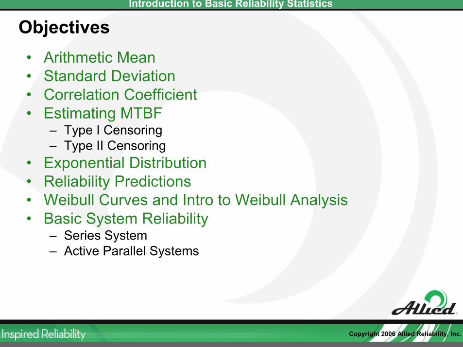
Objectives• Arithmetic Mean• Standard Deviation• Correlation Coefficient• Estimating MTBF
– Type I Censoring– Type II Censoring
• Exponential Distribution• Reliability Predictions• Weibull Curves and Intro to Weibull Analysis• Basic System Reliability
– Series System– Active Parallel Systems
Copyright 2006 Allied Reliability, Inc.
Introduction to Basic Reliability Statistics
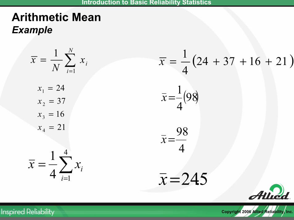
Arithmetic Mean
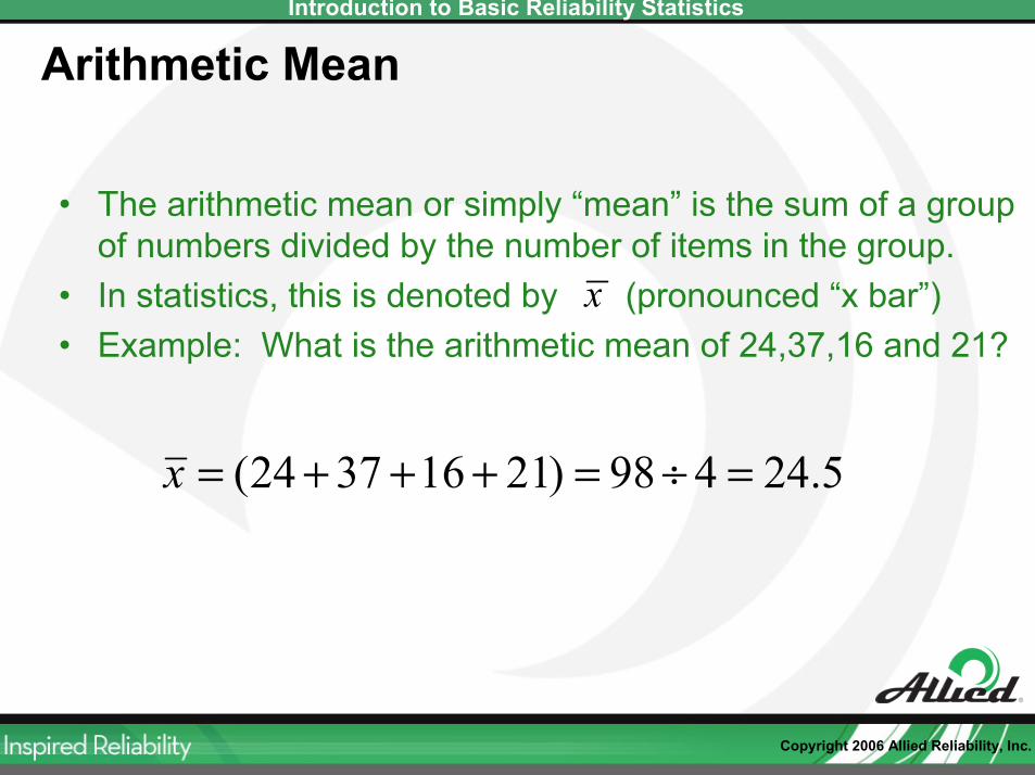
• The arithmetic mean or simply “mean” is the sum of a group of numbers divided by the number of items in the group.
• In statistics, this is denoted by (pronounced “x bar”)• Example: What is the arithmetic mean of 24,37,16 and 21?
x
5.24498)21163724( =÷=+++=x
Copyright 2006 Allied Reliability, Inc.
Introduction to Basic Reliability Statistics
Arithmetic MeanExample
∑=
=N
iixN
x1
1
21163724
4
3
2
1
====
xxxx
∑=
=4
141i
ixx
( )2116372441 +++=x
( )9841=x
498=x
5.24=x
Copyright 2006 Allied Reliability, Inc.
Introduction to Basic Reliability Statistics
Standard Deviation
• Standard deviation is the measure of statistical dispersion in a set of numbers.
• It is the Root Mean Square (RMS) of the deviation from the arithmetic mean of a group of numbers.
• If the data points are all close to the mean then the Standard Deviation is close to zero.
• If the data points are far from the mean then the standard deviation is far from zero.
• Standard deviation is noted by the lower case Greek letter Sigma ( )σ
Copyright 2006 Allied Reliability, Inc.
Introduction to Basic Reliability Statistics
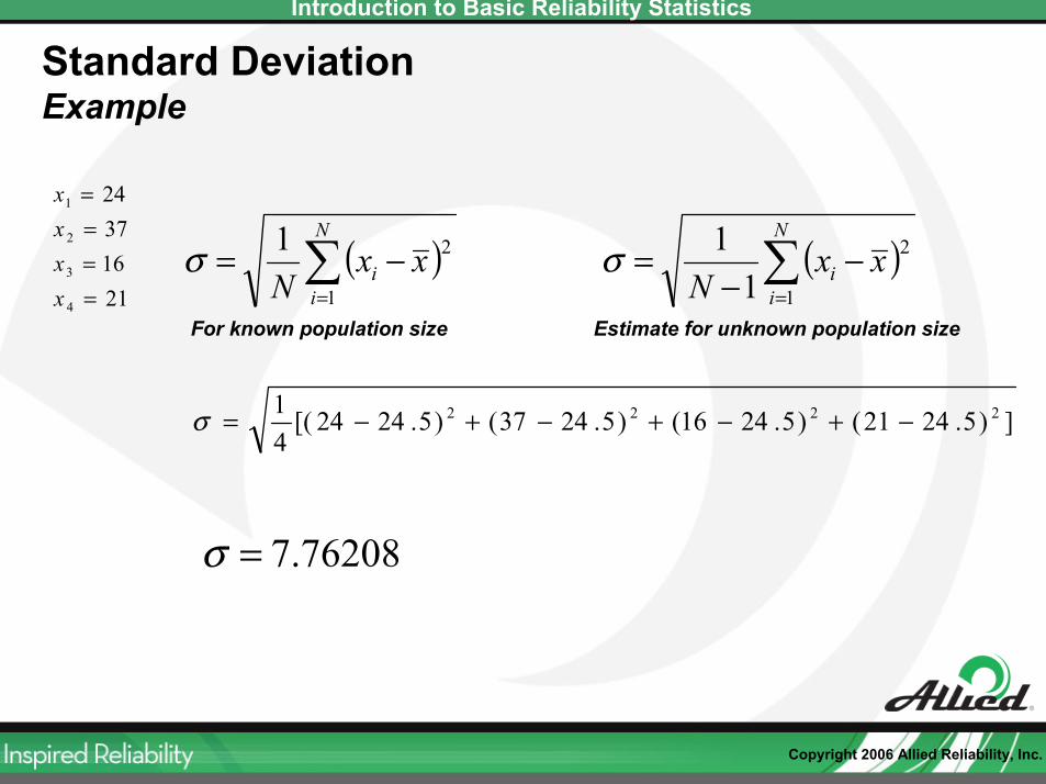
Standard DeviationExample
( )∑=
−=N
ii xx
N 1
21σ21163724
4
3
2
1
====
xxxx
])5.2421()5.2416()5.2437()5.2424[(41 2222 −+−+−+−=σ
76208.7=σ
For known population size
( )∑=
−−
=N
ii xx
N 1
2
11σ
Estimate for unknown population size
Copyright 2006 Allied Reliability, Inc.
Introduction to Basic Reliability Statistics
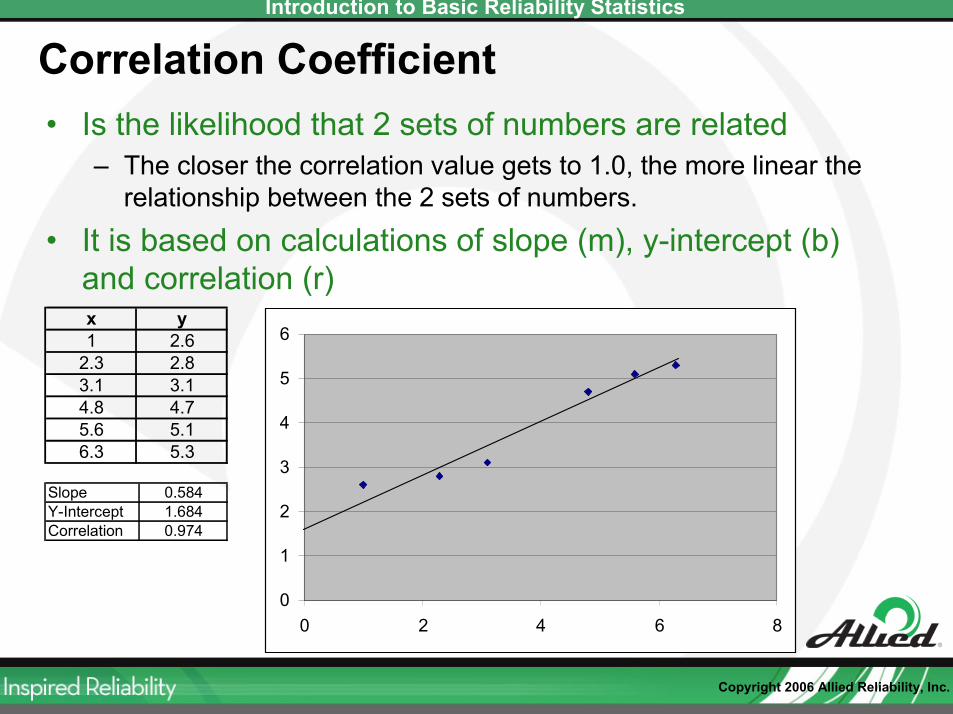
Correlation Coefficient• Is the likelihood that 2 sets of numbers are related
– The closer the correlation value gets to 1.0, the more linear the relationship between the 2 sets of numbers.
• It is based on calculations of slope (m), y-intercept (b) and correlation (r)x y1 2.6
2.3 2.83.1 3.14.8 4.75.6 5.16.3 5.3
0
1
2
3
4
5
6
0 2 4 6 8
Slope 0.584Y-Intercept 1.684Correlation 0.974
Copyright 2006 Allied Reliability, Inc.
Introduction to Basic Reliability Statistics
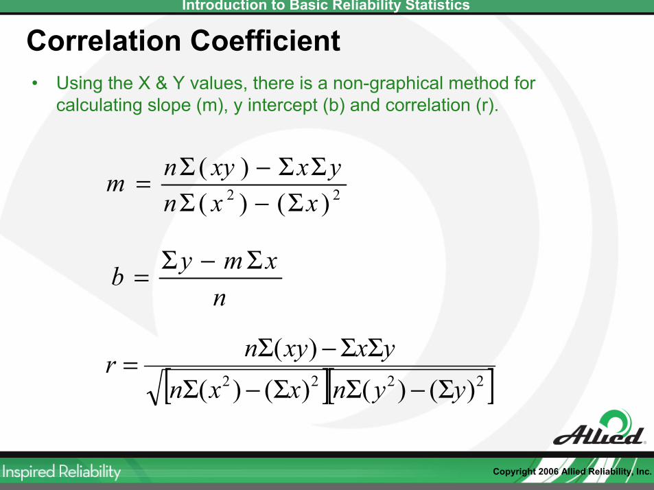
Correlation Coefficient• Using the X & Y values, there is a non-graphical method for
calculating slope (m), y intercept (b) and correlation (r).
22 )()()(
xxnyxxynm
Σ−ΣΣΣ−Σ=
nxmyb Σ−Σ=
[ ][ ]2222 )()()()()(
yynxxnyxxynr
Σ−ΣΣ−ΣΣΣ−Σ=
Copyright 2006 Allied Reliability, Inc.
Introduction to Basic Reliability Statistics
Correlation Coefficient
• Why do I need this? How can I use it?
• Does equipment become more prone to failure or more expensive failures as it ages?– Collect some ages and failure rate data and find out?– Collect some ages and MTBF and find out?
• Other examples:– For a pump, are motor amps and gallons per minute
perfectly linear?

Copyright 2006 Allied Reliability, Inc.
Introduction to Basic Reliability Statistics
Maintenance Costs versus Vibration Analysis (PdM)
Industry: Chemical Processing
Source: 1997 Benchmarking Study in Chemical Processing industry, John Schultz to be featured in Ron Moore’s new book What Tool? When? Selecting the Right Manufacturing Improvement Strategies and Tools
Main
tena
nce C
osts
($)
Vibration Analysis (%)
Copyright 2006 Allied Reliability, Inc.
Introduction to Basic Reliability Statistics
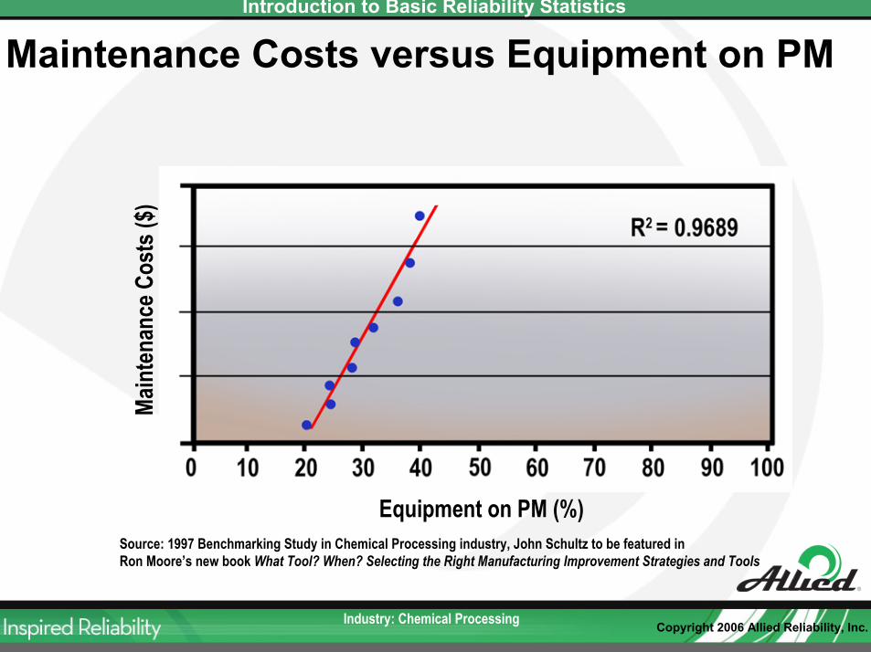
Maintenance Costs versus Equipment on PM
Industry: Chemical Processing
Main
tena
nce C
osts
($)
Equipment on PM (%)Source: 1997 Benchmarking Study in Chemical Processing industry, John Schultz to be featured in Ron Moore’s new book What Tool? When? Selecting the Right Manufacturing Improvement Strategies and Tools
Copyright 2006 Allied Reliability, Inc.
Introduction to Basic Reliability Statistics
Mean Time Between Failures
• MTBF is supposed to be calculated for each individual asset
• Do you calculate it at your plant?
Copyright 2006 Allied Reliability, Inc.
Introduction to Basic Reliability Statistics
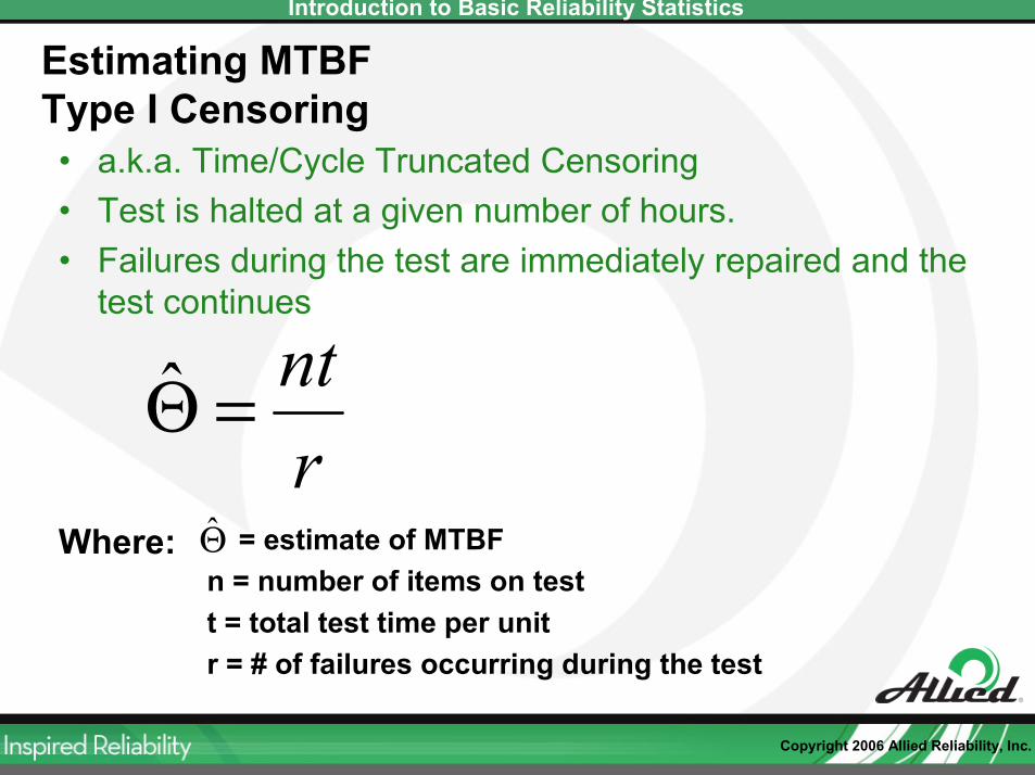
Estimating MTBFType I Censoring• a.k.a. Time/Cycle Truncated Censoring• Test is halted at a given number of hours.• Failures during the test are immediately repaired and the
test continues
rnt=Θ̂
= estimate of MTBFn = number of items on testt = total test time per unitr = # of failures occurring during the test
Θ̂Where:
Copyright 2006 Allied Reliability, Inc.
Introduction to Basic Reliability Statistics
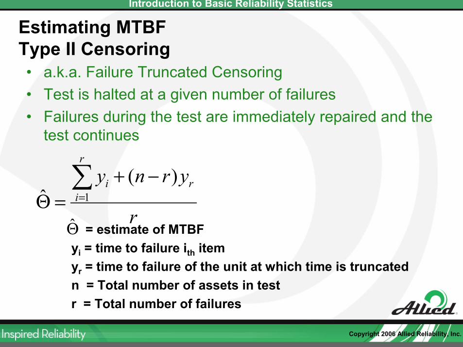
Estimating MTBFType II Censoring• a.k.a. Failure Truncated Censoring• Test is halted at a given number of failures• Failures during the test are immediately repaired and the
test continues
r
yrnyr
iri∑
=
−+=Θ 1
)(ˆ
= estimate of MTBFyi = time to failure ith itemyr = time to failure of the unit at which time is truncatedn = Total number of assets in testr = Total number of failures
Θ̂
Copyright 2006 Allied Reliability, Inc.
Introduction to Basic Reliability Statistics
When would I use MTBF?• Good question!
• MTBF can be used to help determine maintenance intervals.
• There is a significant flaw with this.
• What does the M in MTBF stand for?• What does this implicitly tell you?
Copyright 2006 Allied Reliability, Inc.
Introduction to Basic Reliability Statistics
Reliability Predictions
• If I know a little bit about the MTBF for a particular asset…
• I can make some predictions about the life of that asset.
Copyright 2006 Allied Reliability, Inc.
Introduction to Basic Reliability Statistics
Reliability Predictions
• Q is the probability of failure.
• Q = 1 – R
• So then R is the probability of not failing
Copyright 2006 Allied Reliability, Inc.
Introduction to Basic Reliability Statistics
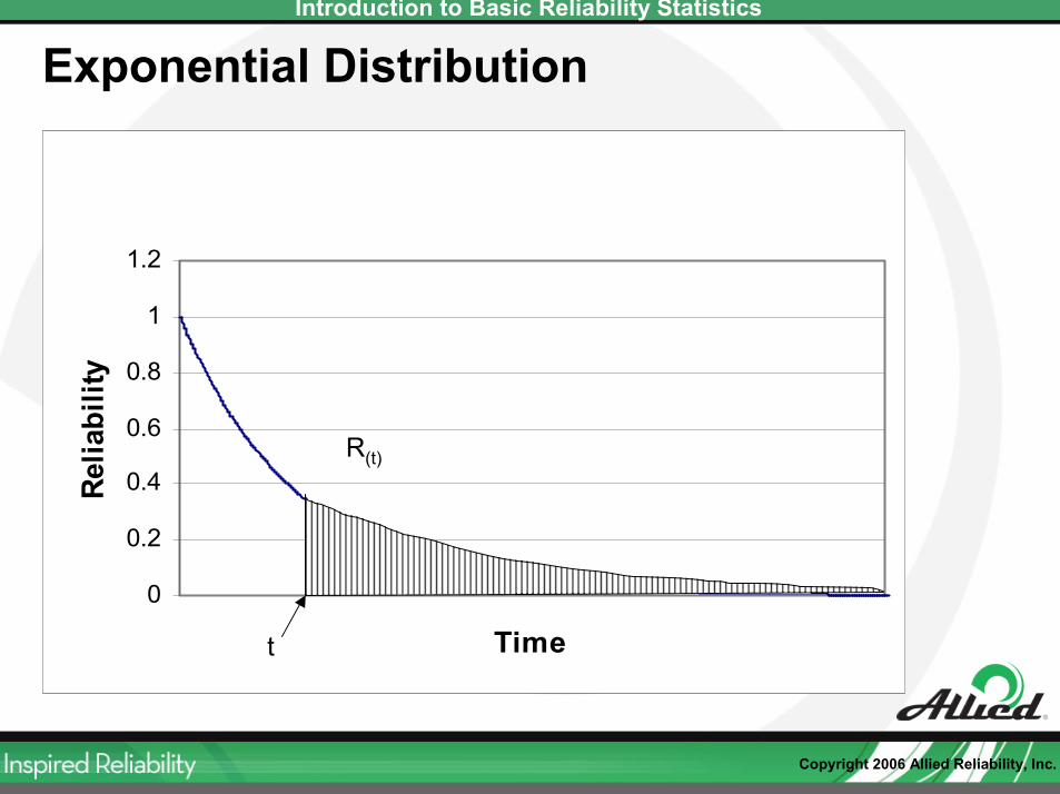
Exponential Distribution
0
0.2
0.4
0.6
0.8
1
1.2
Time
Relia
bilit
y
t
R(t)
Copyright 2006 Allied Reliability, Inc.
Introduction to Basic Reliability Statistics
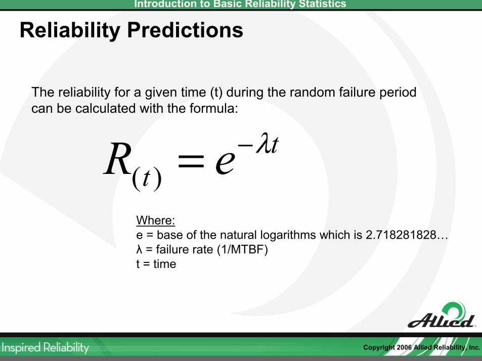
tt eR λ−=)(
The reliability for a given time (t) during the random failure period can be calculated with the formula:
Where:e = base of the natural logarithms which is 2.718281828…λ = failure rate (1/MTBF)t = time
Reliability Predictions
Copyright 2006 Allied Reliability, Inc.
Introduction to Basic Reliability Statistics
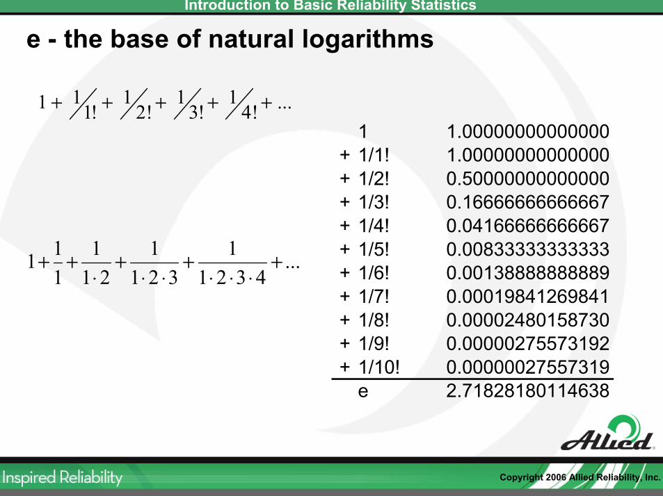
e - the base of natural logarithms
...!41
!31
!21
!111 +++++
...4321
1321
1211
111 +
⋅⋅⋅+
⋅⋅+
⋅++
1 1.00000000000000+ 1/1! 1.00000000000000+ 1/2! 0.50000000000000+ 1/3! 0.16666666666667+ 1/4! 0.04166666666667+ 1/5! 0.00833333333333+ 1/6! 0.00138888888889+ 1/7! 0.00019841269841+ 1/8! 0.00002480158730+ 1/9! 0.00000275573192+ 1/10! 0.00000027557319
e 2.71828180114638
Copyright 2006 Allied Reliability, Inc.
Introduction to Basic Reliability Statistics
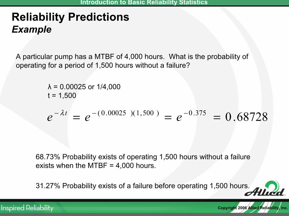
Reliability PredictionsExample
A particular pump has a MTBF of 4,000 hours. What is the probability of operating for a period of 1,500 hours without a failure?
λ = 0.00025 or 1/4,000 t = 1,500
68728.0375.0)500,1)(00025.0( === −−− eee tλ
68.73% Probability exists of operating 1,500 hours without a failureexists when the MTBF = 4,000 hours.
31.27% Probability exists of a failure before operating 1,500 hours.
Copyright 2006 Allied Reliability, Inc.
Introduction to Basic Reliability Statistics
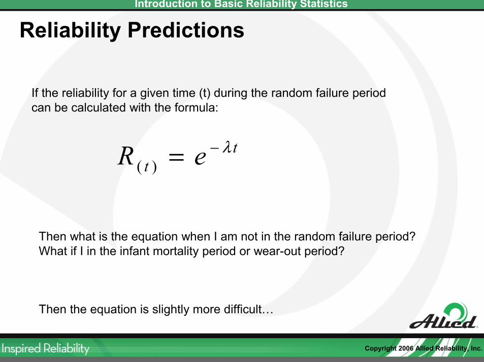
Reliability Predictions
If the reliability for a given time (t) during the random failure period can be calculated with the formula:
tt eR λ−=)(
Then what is the equation when I am not in the random failure period?What if I in the infant mortality period or wear-out period?
Then the equation is slightly more difficult…
Copyright 2006 Allied Reliability, Inc.
Introduction to Basic Reliability Statistics
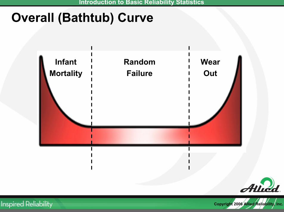
Overall (Bathtub) Curve
InfantMortality
WearOut
RandomFailure
Copyright 2006 Allied Reliability, Inc.
Introduction to Basic Reliability Statistics
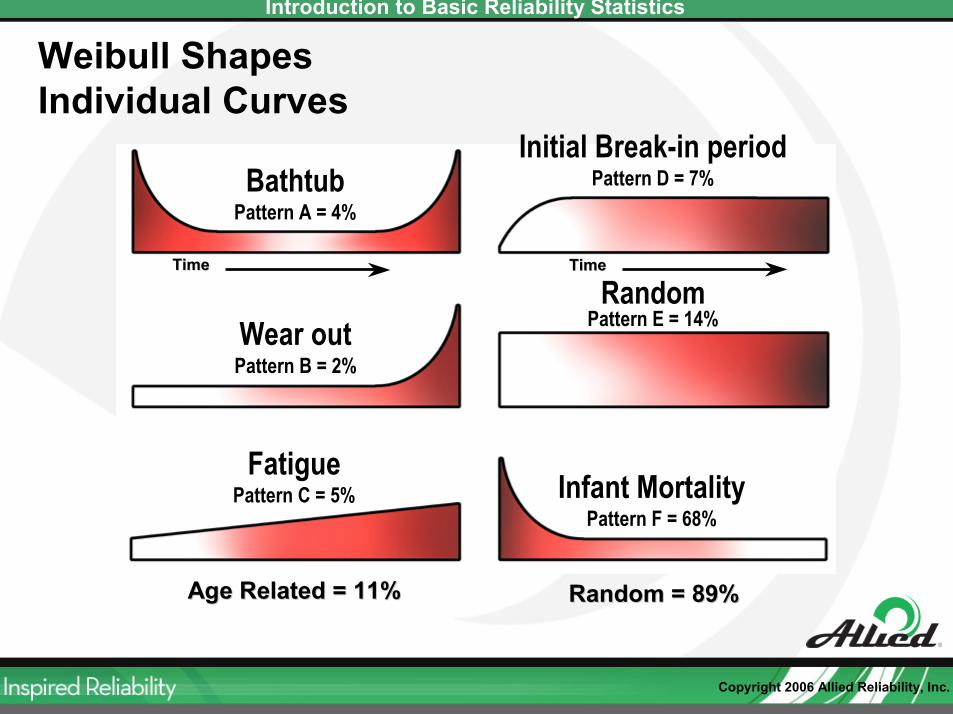
Weibull ShapesIndividual Curves
TimeTime
Age Related = 11%Age Related = 11% Random = 89%Random = 89%
BathtubPattern A = 4%
Wear outPattern B = 2%
FatiguePattern C = 5%
Initial Break-in periodPattern D = 7%
RandomPattern E = 14%
Infant MortalityPattern F = 68%
TimeTime
Copyright 2006 Allied Reliability, Inc.
Introduction to Basic Reliability Statistics
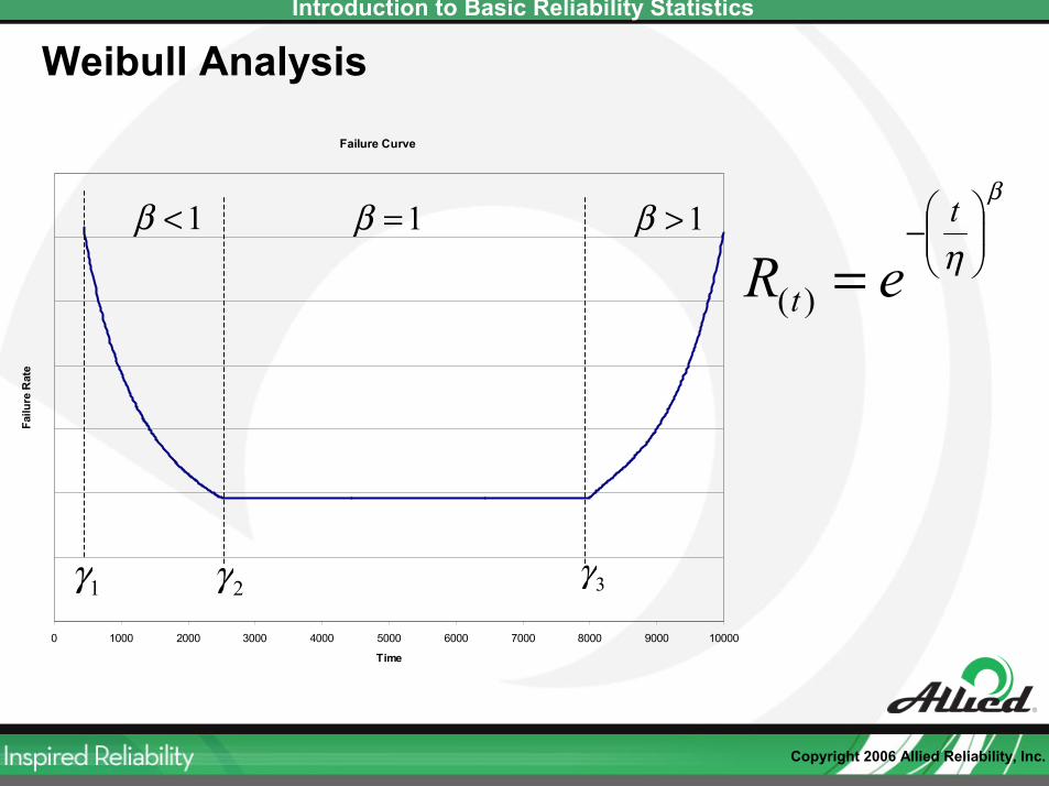
Weibull Analysis
Failure Curve
0 1000 2000 3000 4000 5000 6000 7000 8000 9000 10000
Time
Failu
re R
ate
1<β
1γ 3γ2γ
1=β 1>ββ
η
−=
t
t eR )(
Copyright 2006 Allied Reliability, Inc.
Introduction to Basic Reliability Statistics
System Reliability
• Rarely do assets work alone• Typically they are a part of a system• Systems can many different configurations
– Series– Active Parallel– “Hot” Standby Parallel– “Warm” Standby Parallel– “Cold” Standby Parallel
• Reliability calculations for each of these is slightly different
Copyright 2006 Allied Reliability, Inc.
Introduction to Basic Reliability Statistics
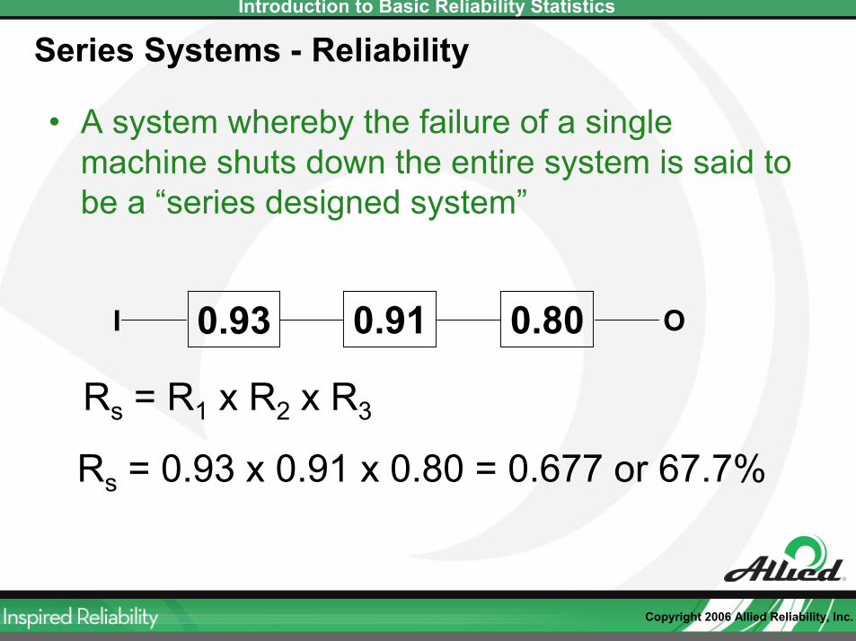
Series Systems - Reliability
• A system whereby the failure of a single machine shuts down the entire system is said to be a “series designed system”
Rs = R1 x R2 x R3
0.93 0.91I O0.80
Rs = 0.93 x 0.91 x 0.80 = 0.677 or 67.7%
Copyright 2006 Allied Reliability, Inc.
Introduction to Basic Reliability Statistics
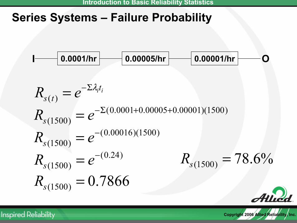
Series Systems – Failure Probability
iitts eR λΣ−=)(
0.0001/hr 0.00005/hrI O0.00001/hr
)1500)(00001.000005.00001.0()1500(
++Σ−= eRs)1500)(00016.0(
)1500(−= eRs
)24.0()1500(
−= eRs7866.0)1500( =sR
%6.78)1500( =sR
Copyright 2006 Allied Reliability, Inc.
Introduction to Basic Reliability Statistics
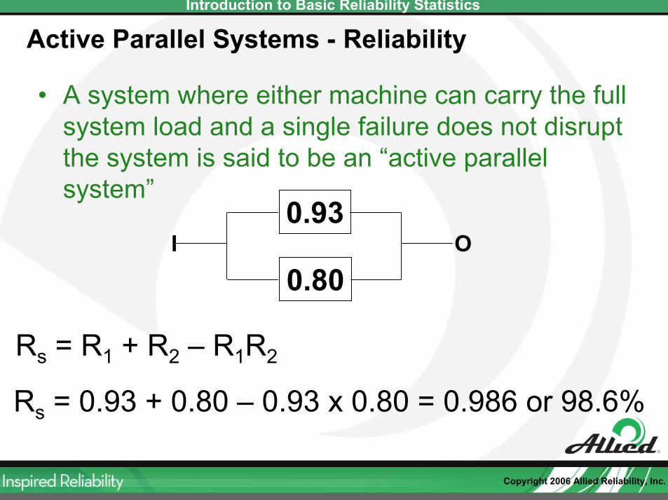
Active Parallel Systems - Reliability
0.93I O
0.80
Rs = R1 + R2 – R1R2
Rs = 0.93 + 0.80 – 0.93 x 0.80 = 0.986 or 98.6%
• A system where either machine can carry the full system load and a single failure does not disrupt the system is said to be an “active parallel system”
Copyright 2006 Allied Reliability, Inc.
Introduction to Basic Reliability Statistics
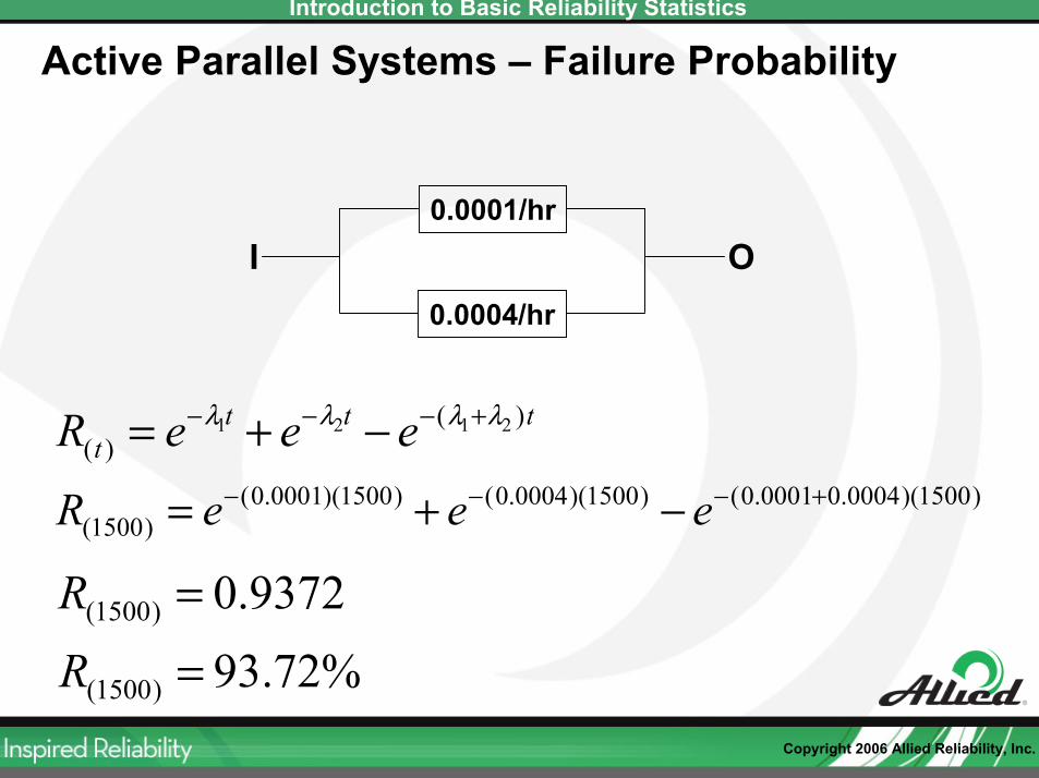
Active Parallel Systems – Failure Probability
tttt eeeR )()(
2121 λλλλ +−−− −+=
0.0001/hrI O
0.0004/hr
)1500)(0004.00001.0()1500)(0004.0()1500)(0001.0()1500(
+−−− −+= eeeR
9372.0)1500( =R%72.93)1500( =R
Copyright 2006 Allied Reliability, Inc.
Introduction to Basic Reliability Statistics
Questions?
Thanks!
James Wheeler, CMRPAllied Reliability