Embed Size (px)
Citation preview
Bayesiananalysis in
Stata
Outline
The generalidea
The MethodBayes rule
Fundamentalequation
MCMC
Stata toolsbayesmh
bayesstats ess
Blocking
bayesgraph
bayes: prefix
bayesstats ic
bayestest model
RandomEffects ProbitThinning
bayestest interval
Change-pointmodelbayesgraph matrix
Summary
References
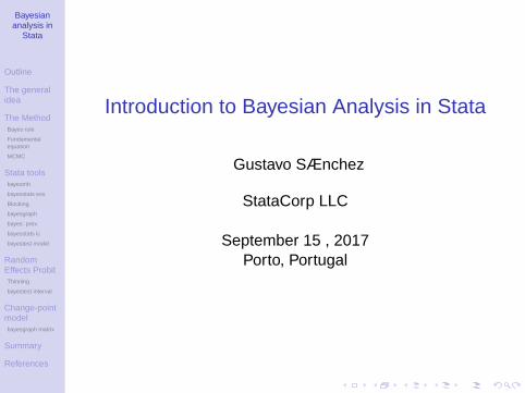
Introduction to Bayesian Analysis in Stata
Gustavo Sánchez
StataCorp LLC
September 15 , 2017Porto, Portugal

Bayesiananalysis in
Stata
Outline
The generalidea
The MethodBayes rule
Fundamentalequation
MCMC
Stata toolsbayesmh
bayesstats ess
Blocking
bayesgraph
bayes: prefix
bayesstats ic
bayestest model
RandomEffects ProbitThinning
bayestest interval
Change-pointmodelbayesgraph matrix
Summary
References
Outline
1 Bayesian analysis: The general idea
2 Basic Concepts• The Method• The tools
• Stata 14: The bayesmh command• Stata 15: The bayes prefix• Postestimation commands
3 A few examples• Linear regression• Panel data random effect probit model• Change point model

Bayesiananalysis in
Stata
Outline
The generalidea
The MethodBayes rule
Fundamentalequation
MCMC
Stata toolsbayesmh
bayesstats ess
Blocking
bayesgraph
bayes: prefix
bayesstats ic
bayestest model
RandomEffects ProbitThinning
bayestest interval
Change-pointmodelbayesgraph matrix
Summary
References
The general idea

Bayesiananalysis in
Stata
Outline
The generalidea
The MethodBayes rule
Fundamentalequation
MCMC
Stata toolsbayesmh
bayesstats ess
Blocking
bayesgraph
bayes: prefix
bayesstats ic
bayestest model
RandomEffects ProbitThinning
bayestest interval
Change-pointmodelbayesgraph matrix
Summary
References
Bayesian Analysis vs Frequentist Analysis
Frequentist Analysis
• Results are based onestimations for unknown fixedparameters.
• The data are considered tobe a (hypothetical)repeatable random sample.
• Uses the data to obtainestimates about the unknownfixed parameters.
• Depends on whether the datasatisfies the assumptions forthe specified model.
"Frequentists base theirconclusions on the distribution ofstatistics derived from randomsamples, assuming that theparameters are unknown butfixed."
Bayesian Analyis
• Results are based onprobability distributions aboutunknown random parameters
• The data are considered tobe fixed.
• The results are produced bycombining the data with priorbeliefs about the parameters.
• The posterior distribution isused to make explicitprobabilistic statements
"Bayesian analysis answersquestions based on the distributionof parameters conditional on theobserved sample."

Bayesiananalysis in
Stata
Outline
The generalidea
The MethodBayes rule
Fundamentalequation
MCMC
Stata toolsbayesmh
bayesstats ess
Blocking
bayesgraph
bayes: prefix
bayesstats ic
bayestest model
RandomEffects ProbitThinning
bayestest interval
Change-pointmodelbayesgraph matrix
Summary
References
Some Advantages
• Based on the Bayes rule, which applies to allparametric models.
• Inference is exact, estimation and prediction are basedon posterior distribution.
• Provides more intuitive interpretation in terms ofprobabilities (e.g Credible intervals).
• It is not limited by the sample size.

Bayesiananalysis in
Stata
Outline
The generalidea
The MethodBayes rule
Fundamentalequation
MCMC
Stata toolsbayesmh
bayesstats ess
Blocking
bayesgraph
bayes: prefix
bayesstats ic
bayestest model
RandomEffects ProbitThinning
bayestest interval
Change-pointmodelbayesgraph matrix
Summary
References
Some Disadvantages
• Subjectivity in specifying prior beliefs.• Computationally challenging.• Setting up a model and performing analysis could be
an involving task.

Bayesiananalysis in
Stata
Outline
The generalidea
The MethodBayes rule
Fundamentalequation
MCMC
Stata toolsbayesmh
bayesstats ess
Blocking
bayesgraph
bayes: prefix
bayesstats ic
bayestest model
RandomEffects ProbitThinning
bayestest interval
Change-pointmodelbayesgraph matrix
Summary
References
Some Examples (Taken from Hahn, 2014)
• TranScan Medical use small dataset and priors basedon previous studies to determine the efficacy of its2000 device for mammografy (FDA 1999).
• homeprice.com.hk used Bayesian analysis for pricinginformation on over a million real state properties inHong Kong and surrounding areas (Shamdasany,2011).
• Researchers in the energy industry have usedBayesian analysis to understand petroleum reservoirparameters (Glinsky and Gunning, 2011).

Bayesiananalysis in
Stata
Outline
The generalidea
The MethodBayes rule
Fundamentalequation
MCMC
Stata toolsbayesmh
bayesstats ess
Blocking
bayesgraph
bayes: prefix
bayesstats ic
bayestest model
RandomEffects ProbitThinning
bayestest interval
Change-pointmodelbayesgraph matrix
Summary
References
The Method
• Let’s start by writing the Bayes’ Rule:
p (B|A) =p (A|B) p (B)
p (A)
Where:p (A|B): conditional probability of A given Bp (B|A): conditional probability of B given A
p (B): marginal probability of Bp (A): marginal probability of A
Bayesiananalysis in
Stata
Outline
The generalidea
The MethodBayes rule
Fundamentalequation
MCMC
Stata toolsbayesmh
bayesstats ess
Blocking
bayesgraph
bayes: prefix
bayesstats ic
bayestest model
RandomEffects ProbitThinning
bayestest interval
Change-pointmodelbayesgraph matrix
Summary
References
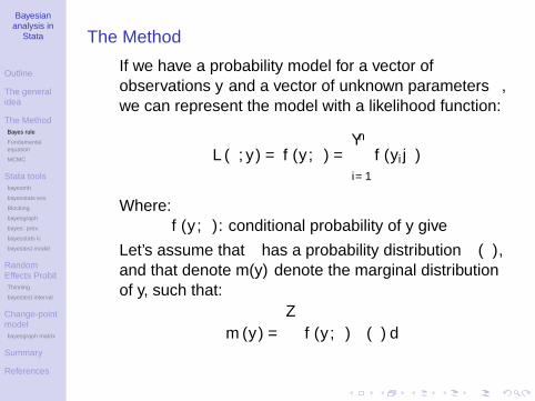
The Method
• If we have a probability model for a vector ofobservations y and a vector of unknown parameters θ,we can represent the model with a likelihood function:
L (θ; y) = f (y ; θ) =n∏
i=1
f (yi |θ)
Where:f (y ; θ): conditional probability of y give θ
• Let’s assume that θ has a probability distribution π (θ),and that denote m(y) denote the marginal distributionof y, such that:
m (y) =
∫f (y ; θ)π (θ) dθ
Bayesiananalysis in
Stata
Outline
The generalidea
The MethodBayes rule
Fundamentalequation
MCMC
Stata toolsbayesmh
bayesstats ess
Blocking
bayesgraph
bayes: prefix
bayesstats ic
bayestest model
RandomEffects ProbitThinning
bayestest interval
Change-pointmodelbayesgraph matrix
Summary
References
The Method
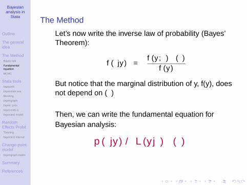
• Let’s now write the inverse law of probability (Bayes’Theorem):
f (θ|y) =f (y ; θ)π (θ)
f (y)
• But notice that the marginal distribution of y, f(y), doesnot depend on (θ)
• Then, we can write the fundamental equation forBayesian analysis:
p (θ|y) ∝ L (y |θ) π (θ)

Bayesiananalysis in
Stata
Outline
The generalidea
The MethodBayes rule
Fundamentalequation
MCMC
Stata toolsbayesmh
bayesstats ess
Blocking
bayesgraph
bayes: prefix
bayesstats ic
bayestest model
RandomEffects ProbitThinning
bayestest interval
Change-pointmodelbayesgraph matrix
Summary
References
Let’s go back to our initial example
Bayesiananalysis in
Stata
Outline
The generalidea
The MethodBayes rule
Fundamentalequation
MCMC
Stata toolsbayesmh
bayesstats ess
Blocking
bayesgraph
bayes: prefix
bayesstats ic
bayestest model
RandomEffects ProbitThinning
bayestest interval
Change-pointmodelbayesgraph matrix
Summary
References
The Method
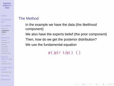
• In the example we have the data (the likelihoodcomponent)
• We also have the experts belief (the prior component)• Then, how do we get the posterior distribution?• We use the fundamental equation
p (θ|y) ∝ L (y |θ)π (θ)
Bayesiananalysis in
Stata
Outline
The generalidea
The MethodBayes rule
Fundamentalequation
MCMC
Stata toolsbayesmh
bayesstats ess
Blocking
bayesgraph
bayes: prefix
bayesstats ic
bayestest model
RandomEffects ProbitThinning
bayestest interval
Change-pointmodelbayesgraph matrix
Summary
References
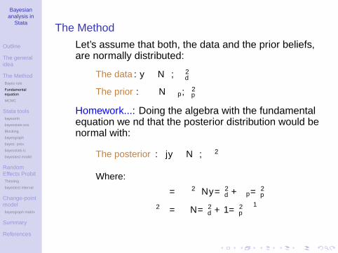
The Method• Let’s assume that both, the data and the prior beliefs,
are normally distributed:
• The data: y ∼ N(θ, σ2
d
)• The prior: θ ∼ N
(µp, σ
2p)
• Homework...: Doing the algebra with the fundamentalequation we find that the posterior distribution would benormal with:
• The posterior: θ|y ∼ N(µ, σ2
)Where:
µ = σ2 (Ny/σ2d + µp/σ
2p)
σ2 =(N/σ2
d + 1/σ2p)−1
Bayesiananalysis in
Stata
Outline
The generalidea
The MethodBayes rule
Fundamentalequation
MCMC
Stata toolsbayesmh
bayesstats ess
Blocking
bayesgraph
bayes: prefix
bayesstats ic
bayestest model
RandomEffects ProbitThinning
bayestest interval
Change-pointmodelbayesgraph matrix
Summary
References
The Method
• Doing the algebra was relatively straightforward in theprevious case.
• What about more complex distributions?• Integration is performed via simulation• We need to use intensive computational simulation
tools to find the posterior distribution in most cases.
• Markov chain Monte Carlo (MCMC) methods are thecurrent standard in most software. Stata implement twoalternatives:
• Metropolis-Hastings (MH) algorithm• Gibbs sampling
Bayesiananalysis in
Stata
Outline
The generalidea
The MethodBayes rule
Fundamentalequation
MCMC
Stata toolsbayesmh
bayesstats ess
Blocking
bayesgraph
bayes: prefix
bayesstats ic
bayestest model
RandomEffects ProbitThinning
bayestest interval
Change-pointmodelbayesgraph matrix
Summary
References
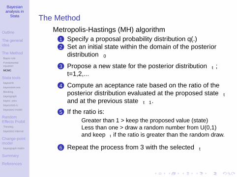
The Method• Metropolis-Hastings (MH) algorithm
1 Specify a proposal probability distribution q(.)2 Set an initial state within the domain of the posterior
distribution θ0
3 Propose a new state for the posterior distribution θt ;t=1,2,...
4 Compute an aceptance rate based on the ratio of theposterior distribution evaluated at the proposed state θtand at the previous state θt−1.
5 If the ratio is:• Greater than 1 –> keep the proposed value (state)• Less than one –> draw a random number from U(0,1)
and keep θt if the ratio is greater than the random draw.
6 Repeat the process from 3 with the selected θt
Bayesiananalysis in
Stata
Outline
The generalidea
The MethodBayes rule
Fundamentalequation
MCMC
Stata toolsbayesmh
bayesstats ess
Blocking
bayesgraph
bayes: prefix
bayesstats ic
bayestest model
RandomEffects ProbitThinning
bayestest interval
Change-pointmodelbayesgraph matrix
Summary
References
The Method
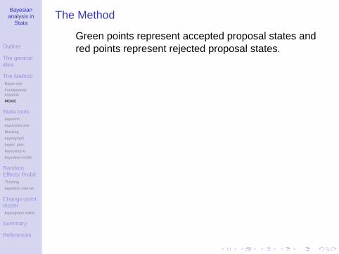
• Green points represent accepted proposal states andred points represent rejected proposal states.
Bayesiananalysis in
Stata
Outline
The generalidea
The MethodBayes rule
Fundamentalequation
MCMC
Stata toolsbayesmh
bayesstats ess
Blocking
bayesgraph
bayes: prefix
bayesstats ic
bayestest model
RandomEffects ProbitThinning
bayestest interval
Change-pointmodelbayesgraph matrix
Summary
References
The Method
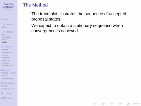
• The trace plot illustrates the sequence of acceptedproposal states.
• We expect to obtain a stationary sequence whenconvergence is achieved.

Bayesiananalysis in
Stata
Outline
The generalidea
The MethodBayes rule
Fundamentalequation
MCMC
Stata toolsbayesmh
bayesstats ess
Blocking
bayesgraph
bayes: prefix
bayesstats ic
bayestest model
RandomEffects ProbitThinning
bayestest interval
Change-pointmodelbayesgraph matrix
Summary
References
The Method
• An efficient MCMC should have small autocorrelation.• We expect autocorrelation to become negligible after a
few lags.

Bayesiananalysis in
Stata
Outline
The generalidea
The MethodBayes rule
Fundamentalequation
MCMC
Stata toolsbayesmh
bayesstats ess
Blocking
bayesgraph
bayes: prefix
bayesstats ic
bayestest model
RandomEffects ProbitThinning
bayestest interval
Change-pointmodelbayesgraph matrix
Summary
References
The Stata tools for Bayesian regression

Bayesiananalysis in
Stata
Outline
The generalidea
The MethodBayes rule
Fundamentalequation
MCMC
Stata toolsbayesmh
bayesstats ess
Blocking
bayesgraph
bayes: prefix
bayesstats ic
bayestest model
RandomEffects ProbitThinning
bayestest interval
Change-pointmodelbayesgraph matrix
Summary
References
The Stata tools: bayesmh
• In Stata 14 we introduce bayesmh.
• This is a general purpose command to perform Bayesiananalysis using MCMC (MH or Gibbs).
• We are going to work with a few examples to show differentfacilities available in Stata for the analysis.
• Let’s look at our first example:
• We have stats on number of wins by the Porto soccer team.
• We fit a linear regression for yearly wins.
• Let’s consider three specifications:
wins = α1 + βgs ∗ goals_scored + ε1
wins = α2 + βga ∗ goals_against + ε2
wins = α3 + βgs2 ∗ goals_scored + βga2 ∗ goals_against + ε3

Bayesiananalysis in
Stata
Outline
The generalidea
The MethodBayes rule
Fundamentalequation
MCMC
Stata toolsbayesmh
bayesstats ess
Blocking
bayesgraph
bayes: prefix
bayesstats ic
bayestest model
RandomEffects ProbitThinning
bayestest interval
Change-pointmodelbayesgraph matrix
Summary
References
The Stata tools: Regression with bayesmh
• Here is one syntax with bayesmh to fit this model:
bayesmh wins gs,likelihood(normal({sigma2})) ///prior({wins:gs _cons}, normal(0,10000)) ///prior({sigma2}, igamma(.01,.01)) ///rseed(123)
• But let’s use the Graphical User Interface (GUI) (Menusand dialog boxes):

Bayesiananalysis in
Stata
Outline
The generalidea
The MethodBayes rule
Fundamentalequation
MCMC
Stata toolsbayesmh
bayesstats ess
Blocking
bayesgraph
bayes: prefix
bayesstats ic
bayestest model
RandomEffects ProbitThinning
bayestest interval
Change-pointmodelbayesgraph matrix
Summary
References
The Stata tools: Menu for Bayesian regression
1 Make the following sequence of selection from the mainmenu:
Statistics > Bayesian analysis> General estimation and regression
2 Select ’Univariate linear models’3 Specify the dependent variable (wins) and the
explanatory variable (gs)
4 Select the ’Likelihood model’ (Normal regression)• For ’Variance’ click on ’Create’ and select ’Specify as a
model parameter’• Type ’sigma2’ in ’Parameter name’
Bayesiananalysis in
Stata
Outline
The generalidea
The MethodBayes rule
Fundamentalequation
MCMC
Stata toolsbayesmh
bayesstats ess
Blocking
bayesgraph
bayes: prefix
bayesstats ic
bayestest model
RandomEffects ProbitThinning
bayestest interval
Change-pointmodelbayesgraph matrix
Summary
References
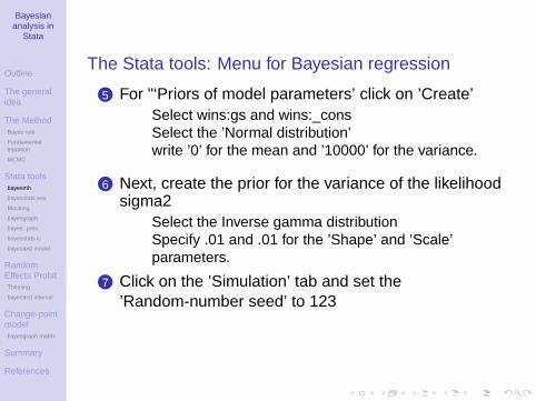
The Stata tools: Menu for Bayesian regression
5 For "‘Priors of model parameters’ click on ’Create’• Select wins:gs and wins:_cons• Select the ’Normal distribution’• write ’0’ for the mean and ’10000’ for the variance.
6 Next, create the prior for the variance of the likelihoodsigma2
• Select the Inverse gamma distribution• Specify .01 and .01 for the ’Shape’ and ’Scale’
parameters.
7 Click on the ’Simulation’ tab and set the’Random-number seed’ to 123

Bayesiananalysis in
Stata
Outline
The generalidea
The MethodBayes rule
Fundamentalequation
MCMC
Stata toolsbayesmh
bayesstats ess
Blocking
bayesgraph
bayes: prefix
bayesstats ic
bayestest model
RandomEffects ProbitThinning
bayestest interval
Change-pointmodelbayesgraph matrix
Summary
References
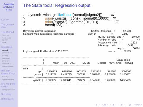
The Stata tools: Regression output
. bayesmh wins gs,likelihood(normal({sigma2})) ///> prior({wins:gs _cons}, normal(0,10000)) ///> prior({sigma2}, igamma(.01,.01)) ///> rseed(123)
Burn-in ...Simulation ...
Model summary
Likelihood:wins ~ normal(xb_wins,{sigma2})
Priors:{wins:gs _cons} ~ normal(0,10000) (1)
{sigma2} ~ igamma(.01,.01)
(1) Parameters are elements of the linear form xb_wins.
Bayesiananalysis in
Stata
Outline
The generalidea
The MethodBayes rule
Fundamentalequation
MCMC
Stata toolsbayesmh
bayesstats ess
Blocking
bayesgraph
bayes: prefix
bayesstats ic
bayestest model
RandomEffects ProbitThinning
bayestest interval
Change-pointmodelbayesgraph matrix
Summary
References
The Stata tools: Regression output
. bayesmh wins gs,likelihood(normal({sigma2})) ///> prior({wins:gs _cons}, normal(0,10000)) ///> prior({sigma2}, igamma(.01,.01)) ///> rseed(123)
Bayesian normal regression MCMC iterations = 12,500Random-walk Metropolis-Hastings sampling Burn-in = 2,500
MCMC sample size = 10,000Number of obs = 47Acceptance rate = .2222Efficiency: min = .04521
avg = .06161Log marginal likelihood = -135.77023 max = .07185
------------------------------------------------------------------------------| Equal-tailed| Mean Std. Dev. MCSE Median [95% Cred. Interval]
-------------+----------------------------------------------------------------wins |
gs | .2360223 .0365801 .001405 .2363132 .162386 .3096086_cons | 6.711756 2.417745 .090197 6.704956 1.923868 11.53032
-------------+----------------------------------------------------------------sigma2 | 9.380877 2.089641 .098277 9.040789 6.262636 14.55403
------------------------------------------------------------------------------
Bayesiananalysis in
Stata
Outline
The generalidea
The MethodBayes rule
Fundamentalequation
MCMC
Stata toolsbayesmh
bayesstats ess
Blocking
bayesgraph
bayes: prefix
bayesstats ic
bayestest model
RandomEffects ProbitThinning
bayestest interval
Change-pointmodelbayesgraph matrix
Summary
References
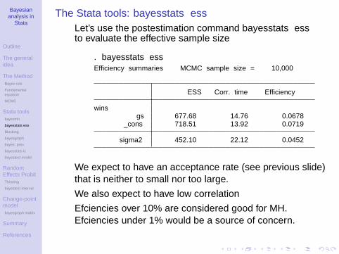
The Stata tools: bayesstats ess
• Let’s use the postestimation command bayesstats essto evaluate the effective sample size
. bayesstats essEfficiency summaries MCMC sample size = 10,000
ESS Corr. time Efficiency
winsgs 677.68 14.76 0.0678
_cons 718.51 13.92 0.0719
sigma2 452.10 22.12 0.0452
• We expect to have an acceptance rate (see previous slide)that is neither to small nor too large.
• We also expect to have low correlation• Efficiencies over 10% are considered good for MH.
Efficiencies under 1% would be a source of concern.
Bayesiananalysis in
Stata
Outline
The generalidea
The MethodBayes rule
Fundamentalequation
MCMC
Stata toolsbayesmh
bayesstats ess
Blocking
bayesgraph
bayes: prefix
bayesstats ic
bayestest model
RandomEffects ProbitThinning
bayestest interval
Change-pointmodelbayesgraph matrix
Summary
References
The Stata tools: Blocking of parameters
• Blocking of parameters
• The update steps for MH are performed simultaneouslyfor all parameters.
• For high dimensional models this may result in poormixing.
• Blocking of parameters helps improving mixingefficiency
Bayesiananalysis in
Stata
Outline
The generalidea
The MethodBayes rule
Fundamentalequation
MCMC
Stata toolsbayesmh
bayesstats ess
Blocking
bayesgraph
bayes: prefix
bayesstats ic
bayestest model
RandomEffects ProbitThinning
bayestest interval
Change-pointmodelbayesgraph matrix
Summary
References
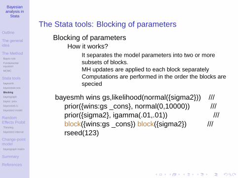
The Stata tools: Blocking of parameters
• Blocking of parameters• How it works?
• It separates the model parameters into two or moresubsets of blocks.
• MH updates are applied to each block separately• Computations are performed in the order the blocks are
specified
bayesmh wins gs,likelihood(normal({sigma2})) ///prior({wins:gs _cons}, normal(0,10000)) ///prior({sigma2}, igamma(.01,.01)) ///block({wins:gs _cons}) block({sigma2}) ///rseed(123)
Bayesiananalysis in
Stata
Outline
The generalidea
The MethodBayes rule
Fundamentalequation
MCMC
Stata toolsbayesmh
bayesstats ess
Blocking
bayesgraph
bayes: prefix
bayesstats ic
bayestest model
RandomEffects ProbitThinning
bayestest interval
Change-pointmodelbayesgraph matrix
Summary
References
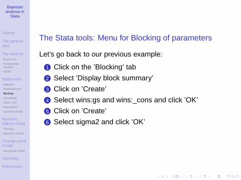
The Stata tools: Menu for Blocking of parameters
Let’s go back to our previous example:
1 Click on the ’Blocking’ tab2 Select ’Display block summary’3 Click on ’Create’4 Select wins:gs and wins:_cons and click ’OK’5 Click on ’Create’6 Select sigma2 and click ’OK’

Bayesiananalysis in
Stata
Outline
The generalidea
The MethodBayes rule
Fundamentalequation
MCMC
Stata toolsbayesmh
bayesstats ess
Blocking
bayesgraph
bayes: prefix
bayesstats ic
bayestest model
RandomEffects ProbitThinning
bayestest interval
Change-pointmodelbayesgraph matrix
Summary
References
The Stata tools: Blocking of parameters
. bayesmh wins gs,likelihood(normal({sigma2})) ///> prior({wins:gs _cons},normal(0,10000)) prior({sigma2},igamma(.01,.01)) ///> block({wins:gs _cons}) block({sigma2}) rseed(123) blocksummary
Burn-in ...Simulation ...
Block summary
1: {wins:gs _cons}2: {sigma2}
Bayesian normal regression MCMC iterations = 12,500Random-walk Metropolis-Hastings sampling Burn-in = 2,500
MCMC sample size = 10,000Number of obs = 47Acceptance rate = .3426Efficiency: min = .09882
avg = .1156Log marginal likelihood = -135.7408 max = .1464
Equal-tailedMean Std. Dev. MCSE Median [95% Cred. Interval]
winsgs .2363963 .0373595 .001188 .2366527 .1626758 .3109461
_cons 6.690619 2.452853 .076957 6.69004 1.683672 11.63661
sigma2 9.392034 2.136876 .05585 9.09526 6.170093 14.36234
Bayesiananalysis in
Stata
Outline
The generalidea
The MethodBayes rule
Fundamentalequation
MCMC
Stata toolsbayesmh
bayesstats ess
Blocking
bayesgraph
bayes: prefix
bayesstats ic
bayestest model
RandomEffects ProbitThinning
bayestest interval
Change-pointmodelbayesgraph matrix
Summary
References
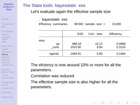
The Stata tools: bayesstats ess
• Let’s evaluate again the effective sample size
. bayesstats essEfficiency summaries MCMC sample size = 10,000
ESS Corr. time Efficiency
winsgs 988.18 10.12 0.0988
_cons 1015.90 9.84 0.1016
sigma2 1463.91 6.83 0.1464
• The efficiency is now around 10% or more for all theparameters.
• Correlation was reduced• The effective sample size is also higher for all the
parameters.

Bayesiananalysis in
Stata
Outline
The generalidea
The MethodBayes rule
Fundamentalequation
MCMC
Stata toolsbayesmh
bayesstats ess
Blocking
bayesgraph
bayes: prefix
bayesstats ic
bayestest model
RandomEffects ProbitThinning
bayestest interval
Change-pointmodelbayesgraph matrix
Summary
References
The Stata tools: bayesgraph
• We can use bayesgraph to look at the trace, thecorrelation, and the density. For example:
. bayesgraph diagnostic {gs}
• The trace indicates that convergence was achieved• Correlation becomes negligible after 10 periods

Bayesiananalysis in
Stata
Outline
The generalidea
The MethodBayes rule
Fundamentalequation
MCMC
Stata toolsbayesmh
bayesstats ess
Blocking
bayesgraph
bayes: prefix
bayesstats ic
bayestest model
RandomEffects ProbitThinning
bayestest interval
Change-pointmodelbayesgraph matrix
Summary
References
The Stata tools: bayes: prefix
• In Stata 15 we introduce the prefix command bayes:
• This is a simple syntax to perform Bayesian analysis.
• You specify the prefix followed by your estimation command.
• The specified estimation defines the likelihood for the model.
• The default priors are assumed to be noninformative in manycases.
• But the priors may become informative due to the scale of theparameters.
• The default priors could be consider a starting point.
• However, alternative priors may need to be considered.
• Postestimation commands would help decide on the finalmodel.
• Let’s use bayes: to fit our previous model:
Bayesiananalysis in
Stata
Outline
The generalidea
The MethodBayes rule
Fundamentalequation
MCMC
Stata toolsbayesmh
bayesstats ess
Blocking
bayesgraph
bayes: prefix
bayesstats ic
bayestest model
RandomEffects ProbitThinning
bayestest interval
Change-pointmodelbayesgraph matrix
Summary
References
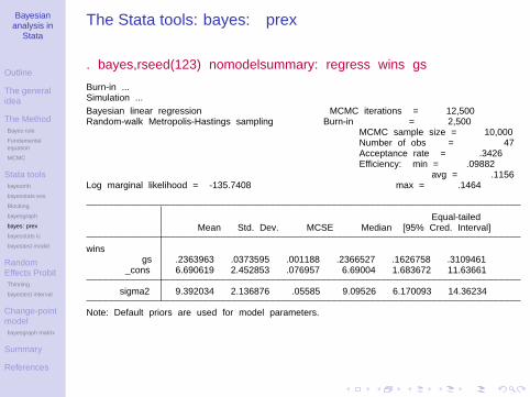
The Stata tools: bayes: prefix
. bayes,rseed(123) nomodelsummary: regress wins gs
Burn-in ...Simulation ...
Bayesian linear regression MCMC iterations = 12,500Random-walk Metropolis-Hastings sampling Burn-in = 2,500
MCMC sample size = 10,000Number of obs = 47Acceptance rate = .3426Efficiency: min = .09882
avg = .1156Log marginal likelihood = -135.7408 max = .1464
Equal-tailedMean Std. Dev. MCSE Median [95% Cred. Interval]
winsgs .2363963 .0373595 .001188 .2366527 .1626758 .3109461
_cons 6.690619 2.452853 .076957 6.69004 1.683672 11.63661
sigma2 9.392034 2.136876 .05585 9.09526 6.170093 14.36234
Note: Default priors are used for model parameters.

Bayesiananalysis in
Stata
Outline
The generalidea
The MethodBayes rule
Fundamentalequation
MCMC
Stata toolsbayesmh
bayesstats ess
Blocking
bayesgraph
bayes: prefix
bayesstats ic
bayestest model
RandomEffects ProbitThinning
bayestest interval
Change-pointmodelbayesgraph matrix
Summary
References
The Stata tools: bayesstats ic
• Let’s fit now the other two models that we specify at thebeginning of this example.
• We will store the results for the three models and we will usethe postestimation command bayesstats ic to select oneof them.
quietly {bayes , rseed(123): regress wins gsestimates store m_gs
bayes , rseed(123): regress wins gaestimates store m_ga
bayes , rseed(123): regress wins gs gaestimates store m_full
}bayesstats ic m_gs m_ga m_full,basemodel(m_ga)
Bayesiananalysis in
Stata
Outline
The generalidea
The MethodBayes rule
Fundamentalequation
MCMC
Stata toolsbayesmh
bayesstats ess
Blocking
bayesgraph
bayes: prefix
bayesstats ic
bayestest model
RandomEffects ProbitThinning
bayestest interval
Change-pointmodelbayesgraph matrix
Summary
References
The Stata tools: bayesstats ic
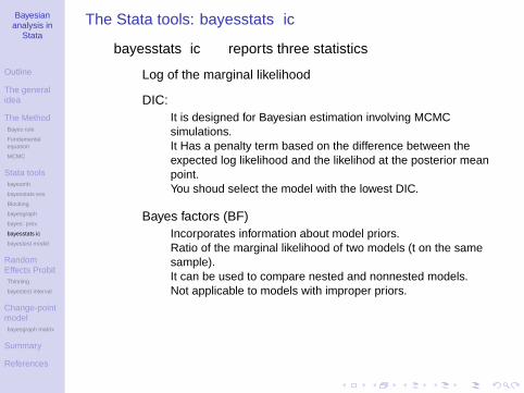
• bayesstats ic reports three statistics
• Log of the marginal likelihood
• DIC:• It is designed for Bayesian estimation involving MCMC
simulations.• It Has a penalty term based on the difference between the
expected log likelihood and the likelihod at the posterior meanpoint.
• You shoud select the model with the lowest DIC.
• Bayes factors (BF)• Incorporates information about model priors.• Ratio of the marginal likelihood of two models (fit on the same
sample).• It can be used to compare nested and nonnested models.• Not applicable to models with improper priors.
Bayesiananalysis in
Stata
Outline
The generalidea
The MethodBayes rule
Fundamentalequation
MCMC
Stata toolsbayesmh
bayesstats ess
Blocking
bayesgraph
bayes: prefix
bayesstats ic
bayestest model
RandomEffects ProbitThinning
bayestest interval
Change-pointmodelbayesgraph matrix
Summary
References
The Stata tools: bayesstats ic
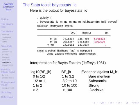
• Here is the output for bayesstats ic
. quietly {
. bayesstats ic m_gs m_ga m_full,basem(m_full) bayesfBayesian information criteria
DIC log(ML) BF
m_gs 240.6314 -135.7408 5.015833m_ga 268.5267 -148.5384 .0000139
m_full 230.9162 -137.3534 .
Note: Marginal likelihood (ML) is computedusing Laplace-Metropolis approximation.
• Interpretation for Bayes Factors (Jeffreys 1961)
log10(BF_jb) BF_jb Evidence against M_b0 to 1/2 1 to 3.2 Bare mention1/2 to 1 3.2 to 10 Substantial1 to 2 10 to 100 Strong> 2 > 100 Decisive
Bayesiananalysis in
Stata
Outline
The generalidea
The MethodBayes rule
Fundamentalequation
MCMC
Stata toolsbayesmh
bayesstats ess
Blocking
bayesgraph
bayes: prefix
bayesstats ic
bayestest model
RandomEffects ProbitThinning
bayestest interval
Change-pointmodelbayesgraph matrix
Summary
References
The Stata tools: bayestest model
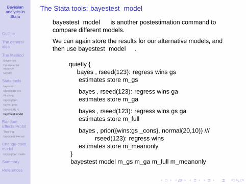
• bayestest model is another postestimation command tocompare different models.
• We can again store the results for our alternative models, andthen use bayestest model.
quietly {bayes , rseed(123): regress wins gsestimates store m_gs
bayes , rseed(123): regress wins gaestimates store m_ga
bayes , rseed(123): regress wins gs gaestimates store m_full
bayes , prior({wins:gs _cons}, normal(20,10)) ///rseed(123): regress wins
estimates store m_meanonly}bayestest model m_gs m_ga m_full m_meanonly
Bayesiananalysis in
Stata
Outline
The generalidea
The MethodBayes rule
Fundamentalequation
MCMC
Stata toolsbayesmh
bayesstats ess
Blocking
bayesgraph
bayes: prefix
bayesstats ic
bayestest model
RandomEffects ProbitThinning
bayestest interval
Change-pointmodelbayesgraph matrix
Summary
References
The Stata tools: bayestest model
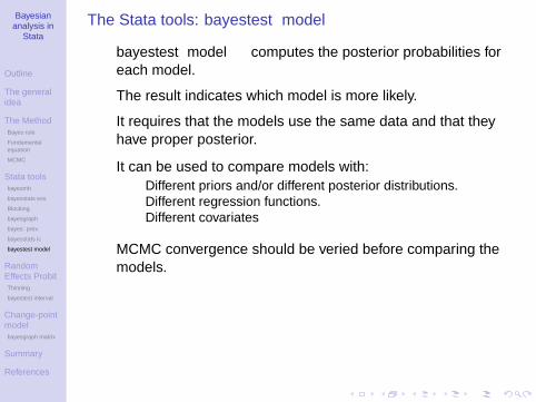
• bayestest model computes the posterior probabilities foreach model.
• The result indicates which model is more likely.
• It requires that the models use the same data and that theyhave proper posterior.
• It can be used to compare models with:• Different priors and/or different posterior distributions.• Different regression functions.• Different covariates
• MCMC convergence should be verified before comparing themodels.
Bayesiananalysis in
Stata
Outline
The generalidea
The MethodBayes rule
Fundamentalequation
MCMC
Stata toolsbayesmh
bayesstats ess
Blocking
bayesgraph
bayes: prefix
bayesstats ic
bayestest model
RandomEffects ProbitThinning
bayestest interval
Change-pointmodelbayesgraph matrix
Summary
References
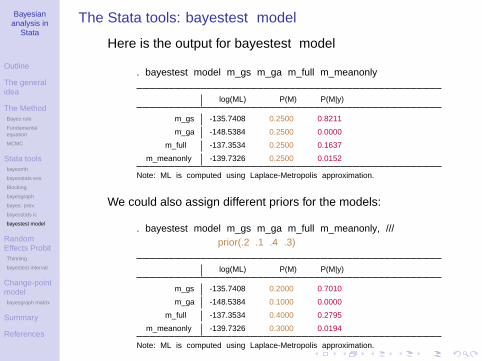
The Stata tools: bayestest model
• Here is the output for bayestest model
. bayestest model m_gs m_ga m_full m_meanonly
log(ML) P(M) P(M|y)
m_gs -135.7408 0.2500 0.8211
m_ga -148.5384 0.2500 0.0000
m_full -137.3534 0.2500 0.1637
m_meanonly -139.7326 0.2500 0.0152
Note: ML is computed using Laplace-Metropolis approximation.
• We could also assign different priors for the models:
. bayestest model m_gs m_ga m_full m_meanonly, ///
prior(.2 .1 .4 .3)
log(ML) P(M) P(M|y)
m_gs -135.7408 0.2000 0.7010
m_ga -148.5384 0.1000 0.0000
m_full -137.3534 0.4000 0.2795
m_meanonly -139.7326 0.3000 0.0194
Note: ML is computed using Laplace-Metropolis approximation.
Bayesiananalysis in
Stata
Outline
The generalidea
The MethodBayes rule
Fundamentalequation
MCMC
Stata toolsbayesmh
bayesstats ess
Blocking
bayesgraph
bayes: prefix
bayesstats ic
bayestest model
RandomEffects ProbitThinning
bayestest interval
Change-pointmodelbayesgraph matrix
Summary
References
Random Effects Probit model
Bayesiananalysis in
Stata
Outline
The generalidea
The MethodBayes rule
Fundamentalequation
MCMC
Stata toolsbayesmh
bayesstats ess
Blocking
bayesgraph
bayes: prefix
bayesstats ic
bayestest model
RandomEffects ProbitThinning
bayestest interval
Change-pointmodelbayesgraph matrix
Summary
References
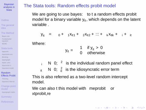
The Stata tools: Random effects probit model
• We are going to use bayes: to fit a random effects probitmodel for a binary variable yit , which depends on the latentvariable .
y∗it = β0 + β1xit1 + β2xit2 + ...+ βkxitk + αi + εit
Where:
yit =
{1 if y∗
it > 00 otherwise
αi ∼ N(0, σ2
α
)is the individual random panel effect
εit ∼ N(0, σ2
e)
is the idiosyncratic error term
• This is also referred as a two-level random interceptmodel.
• We can also fit this model with meprobit orxtprobit,re
Bayesiananalysis in
Stata
Outline
The generalidea
The MethodBayes rule
Fundamentalequation
MCMC
Stata toolsbayesmh
bayesstats ess
Blocking
bayesgraph
bayes: prefix
bayesstats ic
bayestest model
RandomEffects ProbitThinning
bayestest interval
Change-pointmodelbayesgraph matrix
Summary
References
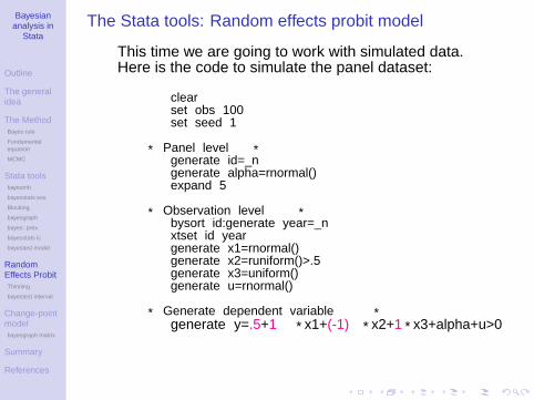
The Stata tools: Random effects probit model
• This time we are going to work with simulated data.• Here is the code to simulate the panel dataset:
clearset obs 100set seed 1
* Panel level *generate id=_ngenerate alpha=rnormal()expand 5
* Observation level *bysort id:generate year=_nxtset id yeargenerate x1=rnormal()generate x2=runiform()>.5generate x3=uniform()generate u=rnormal()
* Generate dependent variable *generate y=.5+1*x1+(-1)*x2+1*x3+alpha+u>0
Bayesiananalysis in
Stata
Outline
The generalidea
The MethodBayes rule
Fundamentalequation
MCMC
Stata toolsbayesmh
bayesstats ess
Blocking
bayesgraph
bayes: prefix
bayesstats ic
bayestest model
RandomEffects ProbitThinning
bayestest interval
Change-pointmodelbayesgraph matrix
Summary
References
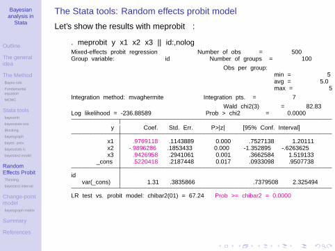
The Stata tools: Random effects probit model
Let’s show the results with meprobit:
. meprobit y x1 x2 x3 || id:,nologMixed-effects probit regression Number of obs = 500Group variable: id Number of groups = 100
Obs per group:min = 5avg = 5.0max = 5
Integration method: mvaghermite Integration pts. = 7
Wald chi2(3) = 82.83Log likelihood = -236.88589 Prob > chi2 = 0.0000
y Coef. Std. Err. P>|z| [95% Conf. Interval]
x1 .9769118 .1143889 0.000 .7527138 1.20111x2 -.9896286 .1853433 0.000 -1.352895 -.6263625x3 .9426958 .2941061 0.001 .3662584 1.519133
_cons .5220418 .2187448 0.017 .0933098 .9507738
idvar(_cons) 1.31 .3835866 .7379508 2.325494
LR test vs. probit model: chibar2(01) = 67.24 Prob >= chibar2 = 0.0000

Bayesiananalysis in
Stata
Outline
The generalidea
The MethodBayes rule
Fundamentalequation
MCMC
Stata toolsbayesmh
bayesstats ess
Blocking
bayesgraph
bayes: prefix
bayesstats ic
bayestest model
RandomEffects ProbitThinning
bayestest interval
Change-pointmodelbayesgraph matrix
Summary
References
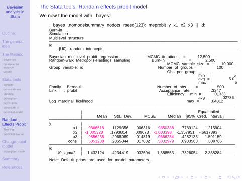
The Stata tools: Random effects probit model
We now fit the model with bayes:
. bayes , dryrun: meprobit y x1 x2 x3 || id:Multilevel structure
id{U0}: random intercepts
Model summary
Likelihood:y ~ meprobit(xb_y)
Priors:{y:x1 x2 x3 _cons} ~ normal(0,10000) (1)
{U0} ~ normal(0,{U0:sigma2}) (1).Hyperprior:
{U0:sigma2} ~ igamma(.01,.01)
(1) Parameters are elements of the linear form xb_y.
Bayesiananalysis in
Stata
Outline
The generalidea
The MethodBayes rule
Fundamentalequation
MCMC
Stata toolsbayesmh
bayesstats ess
Blocking
bayesgraph
bayes: prefix
bayesstats ic
bayestest model
RandomEffects ProbitThinning
bayestest interval
Change-pointmodelbayesgraph matrix
Summary
References
The Stata tools: Random effects probit model
We now fit the model with bayes:
. bayes ,nomodelsummary nodots rseed(123): meprobit y x1 x2 x3 || id:Burn-in ...Simulation ...Multilevel structure
id{U0}: random intercepts
Bayesian multilevel probit regression MCMC iterations = 12,500Random-walk Metropolis-Hastings sampling Burn-in = 2,500
MCMC sample size = 10,000Group variable: id Number of groups = 100
Obs per group:min = 5avg = 5.0max = 5
Family : Bernoulli Number of obs = 500Link : probit Acceptance rate = .3247
Efficiency: min = .01333avg = .02736
Log marginal likelihood max = .04012
Equal-tailedMean Std. Dev. MCSE Median [95% Cred. Interval]
yx1 .9866518 .1129356 .006316 .9850336 .7789124 1.215904x2 -1.005328 .1793814 .009673 -1.003398 -1.357951 -.6617393x3 .9856235 .2968089 .014819 .9666234 .4282133 1.591159
_cons .5051288 .2055344 .017802 .5032979 .0933563 .889766
idU0:sigma2 1.432124 .4234419 .032504 1.388553 .7326054 2.388284
Note: Default priors are used for model parameters.
Bayesiananalysis in
Stata
Outline
The generalidea
The MethodBayes rule
Fundamentalequation
MCMC
Stata toolsbayesmh
bayesstats ess
Blocking
bayesgraph
bayes: prefix
bayesstats ic
bayestest model
RandomEffects ProbitThinning
bayestest interval
Change-pointmodelbayesgraph matrix
Summary
References
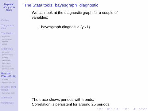
The Stata tools: bayesgraph diagnostic
• We can look at the diagnostic graph for a couple ofvariables:
. bayesgraph diagnostic {y:x1}
• The trace shows periods with trends.• Correlation is persistent for around 25 periods.

Bayesiananalysis in
Stata
Outline
The generalidea
The MethodBayes rule
Fundamentalequation
MCMC
Stata toolsbayesmh
bayesstats ess
Blocking
bayesgraph
bayes: prefix
bayesstats ic
bayestest model
RandomEffects ProbitThinning
bayestest interval
Change-pointmodelbayesgraph matrix
Summary
References
The Stata tools: bayesgraph diagnostic
• Look now at the diagnostic graphs for U0:sigma2
. bayesgraph diagnostic {U0:sigma2}
• The trace also shows periods with trends.• Correlation is persistent for around 30 periods.
Bayesiananalysis in
Stata
Outline
The generalidea
The MethodBayes rule
Fundamentalequation
MCMC
Stata toolsbayesmh
bayesstats ess
Blocking
bayesgraph
bayes: prefix
bayesstats ic
bayestest model
RandomEffects ProbitThinning
bayestest interval
Change-pointmodelbayesgraph matrix
Summary
References
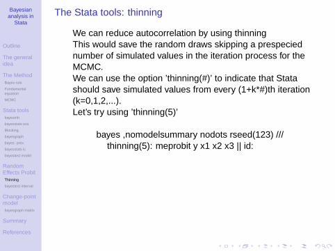
The Stata tools: thinning
• We can reduce autocorrelation by using thinning• This would save the random draws skipping a prespecified
number of simulated values in the iteration process for theMCMC.
• We can use the option ’thinning(#)’ to indicate that Statashould save simulated values from every (1+k*#)th iteration(k=0,1,2,...).
• Let’s try using ’thinning(5)’
bayes ,nomodelsummary nodots rseed(123) ///thinning(5): meprobit y x1 x2 x3 || id:
Bayesiananalysis in
Stata
Outline
The generalidea
The MethodBayes rule
Fundamentalequation
MCMC
Stata toolsbayesmh
bayesstats ess
Blocking
bayesgraph
bayes: prefix
bayesstats ic
bayestest model
RandomEffects ProbitThinning
bayestest interval
Change-pointmodelbayesgraph matrix
Summary
References
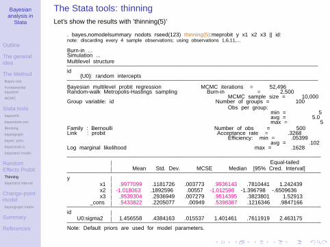
The Stata tools: thinningLet’s show the results with ’thinning(5)’
. bayes,nomodelsummary nodots rseed(123) thinning(5):meprobit y x1 x2 x3 || id:note: discarding every 4 sample observations; using observations 1,6,11,...
Burn-in ...Simulation ...Multilevel structure
id{U0}: random intercepts
Bayesian multilevel probit regression MCMC iterations = 52,496Random-walk Metropolis-Hastings sampling Burn-in = 2,500
MCMC sample size = 10,000Group variable: id Number of groups = 100
Obs per group:min = 5avg = 5.0max = 5
Family : Bernoulli Number of obs = 500Link : probit Acceptance rate = .3268
Efficiency: min = .05399avg = .102
Log marginal likelihood max = .1628
Equal-tailedMean Std. Dev. MCSE Median [95% Cred. Interval]
yx1 .9977099 .1181726 .003773 .9936143 .7810441 1.242439x2 -1.018063 .1892596 .00557 -1.012598 -1.396798 -.6509636x3 .9539304 .2936949 .007279 .9514395 .3823801 1.52913
_cons .5433822 .2205077 .00949 .5398387 .1216346 .9847166
idU0:sigma2 1.456558 .4384163 .015537 1.401461 .7611919 2.463175
Note: Default priors are used for model parameters.
Bayesiananalysis in
Stata
Outline
The generalidea
The MethodBayes rule
Fundamentalequation
MCMC
Stata toolsbayesmh
bayesstats ess
Blocking
bayesgraph
bayes: prefix
bayesstats ic
bayestest model
RandomEffects ProbitThinning
bayestest interval
Change-pointmodelbayesgraph matrix
Summary
References
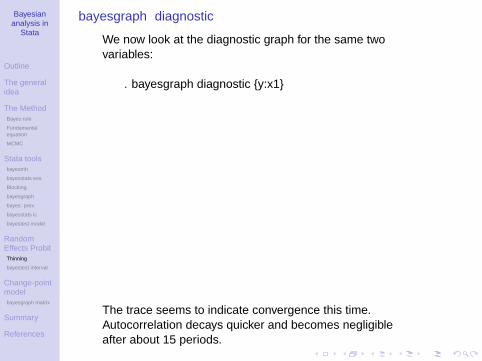
bayesgraph diagnostic
• We now look at the diagnostic graph for the same twovariables:
. bayesgraph diagnostic {y:x1}
• The trace seems to indicate convergence this time.• Autocorrelation decays quicker and becomes negligible
after about 15 periods.

Bayesiananalysis in
Stata
Outline
The generalidea
The MethodBayes rule
Fundamentalequation
MCMC
Stata toolsbayesmh
bayesstats ess
Blocking
bayesgraph
bayes: prefix
bayesstats ic
bayestest model
RandomEffects ProbitThinning
bayestest interval
Change-pointmodelbayesgraph matrix
Summary
References
The Stata tools: bayesgraph diagnostic
• We now look now at the diagnostic graphs for U0:sigma2
. bayesgraph diagnostic {U0:sigma2}
• The trace seems to indicate convergence this time.• Autocorrelation decays quicker and becomes negligible
after about 15 periods.
Bayesiananalysis in
Stata
Outline
The generalidea
The MethodBayes rule
Fundamentalequation
MCMC
Stata toolsbayesmh
bayesstats ess
Blocking
bayesgraph
bayes: prefix
bayesstats ic
bayestest model
RandomEffects ProbitThinning
bayestest interval
Change-pointmodelbayesgraph matrix
Summary
References
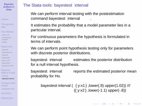
The Stata tools: bayestest interval
• We can perform interval testing with the postestimationcommand bayestest interval.
• It estimates the probability that a model parameter lies in aparticular interval.
• For continuous parameters the hypothesis is formulated interms of intervals.
• We can perform point hypothesis testing only for parameterswith discrete posterior distributions.
• bayestest interval estimates the posterior distributionfor a null interval hypothesis.
• bayestest interval reports the estimated posterior meanprobability for Ho.
bayestest interval ({y:x1},lower(.9) upper(1.02)) ///({y:x2},lower(-1.1) upper(-.8))

Bayesiananalysis in
Stata
Outline
The generalidea
The MethodBayes rule
Fundamentalequation
MCMC
Stata toolsbayesmh
bayesstats ess
Blocking
bayesgraph
bayes: prefix
bayesstats ic
bayestest model
RandomEffects ProbitThinning
bayestest interval
Change-pointmodelbayesgraph matrix
Summary
References
The Stata tools: bayestest interval
• We can, for example, perform separate tests fordifferent parameters:
. bayestest interval ({y:x1},lower(.9) upper(1.02)) ///> ({y:x2},lower(-1.1) upper(-.8))
Interval tests MCMC sample size = 10,000
prob1 : .9 < {y:x1} < 1.02prob2 : -1.1 < {y:x2} < -.8
Mean Std. Dev. MCSE
prob1 .3888 0.48750 .0077073prob2 .5474 0.49777 .0097517
• We can also perform a joint test:
. bayestest interval (({y:x1},lower(.9) upper(1.02)) ///> ({y:x2},lower(-1.1) upper(-.8)),joint)
Interval tests MCMC sample size = 10,000
prob1 : .9 < {y:x1} < 1.02, -1.1 < {y:x2} < -.8
Mean Std. Dev. MCSE
prob1 .2249 0.41754 .0066399
Bayesiananalysis in
Stata
Outline
The generalidea
The MethodBayes rule
Fundamentalequation
MCMC
Stata toolsbayesmh
bayesstats ess
Blocking
bayesgraph
bayes: prefix
bayesstats ic
bayestest model
RandomEffects ProbitThinning
bayestest interval
Change-pointmodelbayesgraph matrix
Summary
References
Change-point model
Bayesiananalysis in
Stata
Outline
The generalidea
The MethodBayes rule
Fundamentalequation
MCMC
Stata toolsbayesmh
bayesstats ess
Blocking
bayesgraph
bayes: prefix
bayesstats ic
bayestest model
RandomEffects ProbitThinning
bayestest interval
Change-pointmodelbayesgraph matrix
Summary
References
The Stata tools: Change-point model
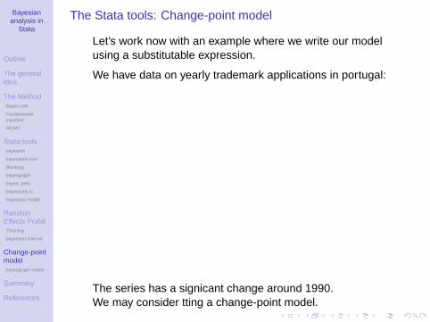
• Let’s work now with an example where we write our modelusing a substitutable expression.
• We have data on yearly trademark applications in portugal:
• The series has a significant change around 1990.• We may consider fitting a change-point model.
Bayesiananalysis in
Stata
Outline
The generalidea
The MethodBayes rule
Fundamentalequation
MCMC
Stata toolsbayesmh
bayesstats ess
Blocking
bayesgraph
bayes: prefix
bayesstats ic
bayestest model
RandomEffects ProbitThinning
bayestest interval
Change-pointmodelbayesgraph matrix
Summary
References
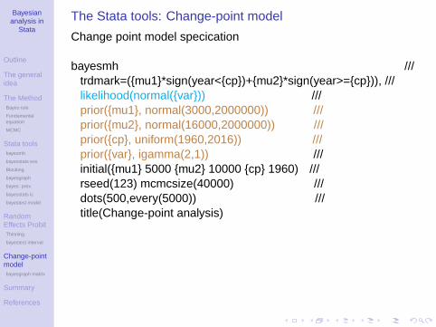
The Stata tools: Change-point model
Change point model specification
bayesmh ///trdmark=({mu1}*sign(year<{cp})+{mu2}*sign(year>={cp})), ///likelihood(normal({var})) ///prior({mu1}, normal(3000,2000000)) ///prior({mu2}, normal(16000,2000000)) ///prior({cp}, uniform(1960,2016)) ///prior({var}, igamma(2,1)) ///initial({mu1} 5000 {mu2} 10000 {cp} 1960) ///rseed(123) mcmcsize(40000) ///dots(500,every(5000)) ///title(Change-point analysis)

Bayesiananalysis in
Stata
Outline
The generalidea
The MethodBayes rule
Fundamentalequation
MCMC
Stata toolsbayesmh
bayesstats ess
Blocking
bayesgraph
bayes: prefix
bayesstats ic
bayestest model
RandomEffects ProbitThinning
bayestest interval
Change-pointmodelbayesgraph matrix
Summary
References
The Stata tools: Change-point modelChange point model specification
. bayesmh trdmark=({mu1}*sign(year<{cp})+{mu2}*sign(year>={cp})), ///> likelihood(normal({var})) ///> prior({mu1}, normal(3000,2000000)) ///> prior({mu2}, normal(16000,2000000)) ///> prior({cp}, uniform(1960,2016)) ///> prior({var}, igamma(2,1)) ///> initial({mu1} 5000 {mu2} 10000 {cp} 1960) ///> rseed(123) mcmcsize(40000) dots(500,every(5000)) ///> title(Change-point analysis)
Burn-in 2500 aaaaa doneSimulation 40000 .........5000.........10000.........15000.........20000> .........25000.........30000.........35000.........40000 done
Model summary
Likelihood:trdmark ~ normal({mu1}*sign(year<{cp})+{mu2}*sign(year>={cp}),{var})
Priors:{var} ~ igamma(2,1){mu1} ~ normal(3000,2000000){mu2} ~ normal(16000,2000000){cp} ~ uniform(1960,2016)

Bayesiananalysis in
Stata
Outline
The generalidea
The MethodBayes rule
Fundamentalequation
MCMC
Stata toolsbayesmh
bayesstats ess
Blocking
bayesgraph
bayes: prefix
bayesstats ic
bayestest model
RandomEffects ProbitThinning
bayestest interval
Change-pointmodelbayesgraph matrix
Summary
References
The Stata tools: Change-point modelChange point model specification
. bayesmh trdmark=({mu1}*sign(year<{cp})+{mu2}*sign(year>={cp})), ///> likelihood(normal({var})) ///> prior({mu1}, normal(3000,2000000)) ///> prior({mu2}, normal(16000,2000000)) ///> prior({cp}, uniform(1960,2016)) ///> prior({var}, igamma(2,1)) ///> initial({mu1} 5000 {mu2} 10000 {cp} 1960) ///> rseed(123) mcmcsize(40000) dots(500,every(5000)) ///> title(Change-point analysis)
Change-point analysis MCMC iterations = 42,500Random-walk Metropolis-Hastings sampling Burn-in = 2,500
MCMC sample size = 40,000Number of obs = 55Acceptance rate = .4117Efficiency: min = .001033
avg = .03796Log marginal likelihood = -621.28408 max = .1362
Equal-tailedMean Std. Dev. MCSE Median [95% Cred. Interval]
cp 1989.492 .2891978 .003918 1989.492 1989.023 1989.972mu1 3754.837 153.0364 11.9209 3761.923 3468.338 4015.751mu2 17448.84 144.531 7.04777 17448.23 17170.98 17736.22var 463983.1 144106.8 22418.1 487445.9 89224.3 621052.3
Note: There is a high autocorrelation after 500 lags.Note: Adaptation tolerance is not met.
Bayesiananalysis in
Stata
Outline
The generalidea
The MethodBayes rule
Fundamentalequation
MCMC
Stata toolsbayesmh
bayesstats ess
Blocking
bayesgraph
bayes: prefix
bayesstats ic
bayestest model
RandomEffects ProbitThinning
bayestest interval
Change-pointmodelbayesgraph matrix
Summary
References
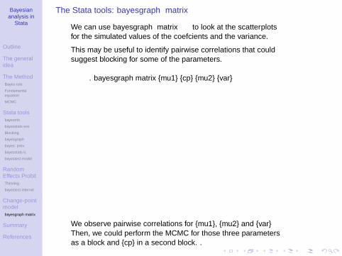
The Stata tools: bayesgraph matrix
• We can use bayesgraph matrix to look at the scatterplotsfor the simulated values of the coefficients and the variance.
• This may be useful to identify pairwise correlations that couldsuggest blocking for some of the parameters.
. bayesgraph matrix {mu1} {cp} {mu2} {var}
• We observe pairwise correlations for {mu1}, {mu2} and {var}• Then, we could perform the MCMC for those three parameters
as a block and {cp} in a second block. .

Bayesiananalysis in
Stata
Outline
The generalidea
The MethodBayes rule
Fundamentalequation
MCMC
Stata toolsbayesmh
bayesstats ess
Blocking
bayesgraph
bayes: prefix
bayesstats ic
bayestest model
RandomEffects ProbitThinning
bayestest interval
Change-pointmodelbayesgraph matrix
Summary
References
The Stata tools: bayesgraph trace
• We can use bayesgraph trace to look at the trace for allthe parameters.
• This helps in determining convergence.
. bayesgraph trace
• We observe signs of lack of convergence, particularly for thevariance.
Bayesiananalysis in
Stata
Outline
The generalidea
The MethodBayes rule
Fundamentalequation
MCMC
Stata toolsbayesmh
bayesstats ess
Blocking
bayesgraph
bayes: prefix
bayesstats ic
bayestest model
RandomEffects ProbitThinning
bayestest interval
Change-pointmodelbayesgraph matrix
Summary
References
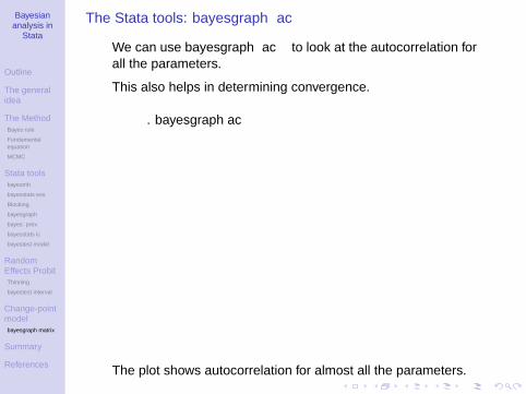
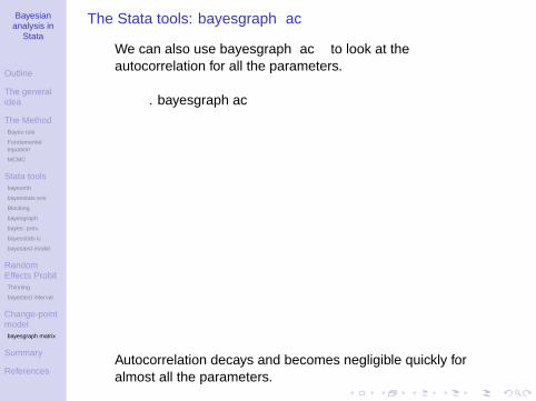
The Stata tools: bayesgraph ac
• We can use bayesgraph ac to look at the autocorrelation forall the parameters.
• This also helps in determining convergence.
. bayesgraph ac
• The plot shows autocorrelation for almost all the parameters.
Bayesiananalysis in
Stata
Outline
The generalidea
The MethodBayes rule
Fundamentalequation
MCMC
Stata toolsbayesmh
bayesstats ess
Blocking
bayesgraph
bayes: prefix
bayesstats ic
bayestest model
RandomEffects ProbitThinning
bayestest interval
Change-pointmodelbayesgraph matrix
Summary
References
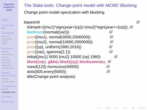
The Stata tools: Change-point model with MCMC Blocking
Change point model specification with blocking
bayesmh ///trdmark=({mu1}*sign(year<{cp})+{mu2}*sign(year>={cp})), ///likelihood(normal({var})) ///prior({mu1}, normal(3000,2000000)) ///prior({mu2}, normal(10000,2000000)) ///prior({cp}, uniform(1960,2016)) ///prior({var}, igamma(2,1)) ///initial({mu1} 5000 {mu2} 10000 {cp} 1960) ///block({var}, gibbs) block({cp}) blocksummary ///rseed(123) mcmcsize(40000) ///dots(500,every(5000)) ///title(Change-point analysis)
Bayesiananalysis in
Stata
Outline
The generalidea
The MethodBayes rule
Fundamentalequation
MCMC
Stata toolsbayesmh
bayesstats ess
Blocking
bayesgraph
bayes: prefix
bayesstats ic
bayestest model
RandomEffects ProbitThinning
bayestest interval
Change-pointmodelbayesgraph matrix
Summary
References
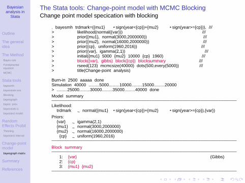
The Stata tools: Change-point model with MCMC BlockingChange point model specification with blocking
. bayesmh trdmark=({mu1}*sign(year<{cp})+{mu2}*sign(year>={cp})), ///> likelihood(normal({var})) ///> prior({mu1}, normal(3000,2000000)) ///> prior({mu2}, normal(16000,2000000)) ///> prior({cp}, uniform(1960,2016)) ///> prior({var}, igamma(2,1)) ///> initial({mu1} 5000 {mu2} 10000 {cp} 1960) ///> block({var}, gibbs) block({cp}) blocksummary ///> rseed(123) mcmcsize(40000) dots(500,every(5000)) ///> title(Change-point analysis)
Burn-in 2500 aaaaa doneSimulation 40000 .........5000.........10000.........15000.........20000> .........25000.........30000.........35000.........40000 done
Model summary
Likelihood:trdmark ~ normal({mu1}*sign(year<{cp})+{mu2}*sign(year>={cp}),{var})
Priors:{var} ~ igamma(2,1){mu1} ~ normal(3000,2000000){mu2} ~ normal(16000,2000000){cp} ~ uniform(1960,2016)
Block summary
1: {var} (Gibbs)2: {cp}3: {mu1} {mu2}
Bayesiananalysis in
Stata
Outline
The generalidea
The MethodBayes rule
Fundamentalequation
MCMC
Stata toolsbayesmh
bayesstats ess
Blocking
bayesgraph
bayes: prefix
bayesstats ic
bayestest model
RandomEffects ProbitThinning
bayestest interval
Change-pointmodelbayesgraph matrix
Summary
References
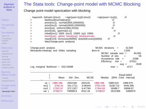
The Stata tools: Change-point model with MCMC BlockingChange point model specification with blocking
. bayesmh trdmark=({mu1}*sign(year<{cp})+{mu2}*sign(year>={cp})), ///> likelihood(normal({var})) ///> prior({mu1}, normal(3000,2000000)) ///> prior({mu2}, normal(16000,2000000)) ///> prior({cp}, uniform(1960,2016)) ///> prior({var}, igamma(2,1)) ///> initial({mu1} 5000 {mu2} 10000 {cp} 1960) ///> block({var}, gibbs) block({cp}) blocksummary ///> rseed(123) mcmcsize(40000) dots(500,every(5000)) ///> title(Change-point analysis)
Change-point analysis MCMC iterations = 42,500Metropolis-Hastings and Gibbs sampling Burn-in = 2,500
MCMC sample size = 40,000Number of obs = 55Acceptance rate = .5288Efficiency: min = .07912
avg = .2638Log marginal likelihood = -533.33098 max = .6717
------------------------------------------------------------------------------| Equal-tailed| Mean Std. Dev. MCSE Median [95% Cred. Interval]
-------------+----------------------------------------------------------------cp | 1989.496 .2944166 .003126 1989.496 1989.019 1989.975mu1 | 3780.26 341.1711 6.06443 3783.149 3108.712 4446.395mu2 | 17332.57 372.1327 6.47794 17344.63 16588.7 18068.87var | 3798272 739589.8 4512.18 3708037 2612399 5480970
------------------------------------------------------------------------------
Bayesiananalysis in
Stata
Outline
The generalidea
The MethodBayes rule
Fundamentalequation
MCMC
Stata toolsbayesmh
bayesstats ess
Blocking
bayesgraph
bayes: prefix
bayesstats ic
bayestest model
RandomEffects ProbitThinning
bayestest interval
Change-pointmodelbayesgraph matrix
Summary
References
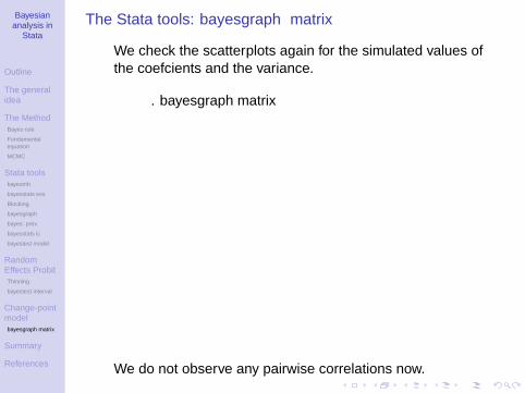
The Stata tools: bayesgraph matrix
• We check the scatterplots again for the simulated values ofthe coefficients and the variance.
. bayesgraph matrix
• We do not observe any pairwise correlations now.

Bayesiananalysis in
Stata
Outline
The generalidea
The MethodBayes rule
Fundamentalequation
MCMC
Stata toolsbayesmh
bayesstats ess
Blocking
bayesgraph
bayes: prefix
bayesstats ic
bayestest model
RandomEffects ProbitThinning
bayestest interval
Change-pointmodelbayesgraph matrix
Summary
References
The Stata tools: bayesgraph trace
• We can use bayesgraph trace to look at the trace for allthe parameters.
. bayesgraph trace
• The plots indicate that convergence seems to be achieved.
Bayesiananalysis in
Stata
Outline
The generalidea
The MethodBayes rule
Fundamentalequation
MCMC
Stata toolsbayesmh
bayesstats ess
Blocking
bayesgraph
bayes: prefix
bayesstats ic
bayestest model
RandomEffects ProbitThinning
bayestest interval
Change-pointmodelbayesgraph matrix
Summary
References
The Stata tools: bayesgraph ac
• We can also use bayesgraph ac to look at theautocorrelation for all the parameters.
. bayesgraph ac
• Autocorrelation decays and becomes negligible quickly foralmost all the parameters.
Bayesiananalysis in
Stata
Outline
The generalidea
The MethodBayes rule
Fundamentalequation
MCMC
Stata toolsbayesmh
bayesstats ess
Blocking
bayesgraph
bayes: prefix
bayesstats ic
bayestest model
RandomEffects ProbitThinning
bayestest interval
Change-pointmodelbayesgraph matrix
Summary
References
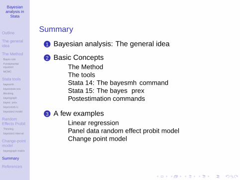
Summary
1 Bayesian analysis: The general idea
2 Basic Concepts• The Method• The tools• Stata 14: The bayesmh command• Stata 15: The bayes prefix• Postestimation commands
3 A few examples• Linear regression• Panel data random effect probit model• Change point model

Bayesiananalysis in
Stata
Outline
The generalidea
The MethodBayes rule
Fundamentalequation
MCMC
Stata toolsbayesmh
bayesstats ess
Blocking
bayesgraph
bayes: prefix
bayesstats ic
bayestest model
RandomEffects ProbitThinning
bayestest interval
Change-pointmodelbayesgraph matrix
Summary
References
References
Glinsky, M. E. and Gunnin, J. 2011. Understanding uncertainty in GSEM.World Oil, 232(1), 57—62, Jan. http://www.worldoil.com/Understanding-uncertainty-in-CSEM-January-2011.html,assessed-Jan.18,2012.
Hahn, Eugene D. 2014. Bayesian Methods for Management andBusiness: Pragmatic Solutions for Real Problems. John Wiley and Sons.
Shamdasany, P. 2011. Smart Money. South China Morning Post. p. 2.,Jul. 4.