Embed Size (px)
Citation preview
1
Introduction to CAD/CAM
IITK ME 761A Dr. J. Ramkumar

2
• CAD can be defined as the use of computer systems to perform
certain functions in the design process.
• CAM is the use of computer systems to plan, manage and control
the operations of manufacturing plant through either direct or
indirect computer interface with the plant’s production resources.
IITK ME 761A Dr. J. Ramkumar

3
From CAM definition, the application of CAM falls into
two broad categories:
1. Computer monitoring and control .
Computer ProcessProcess data
Control signals
Computer ProcessProcess data
IITK ME 761A Dr. J. Ramkumar
4
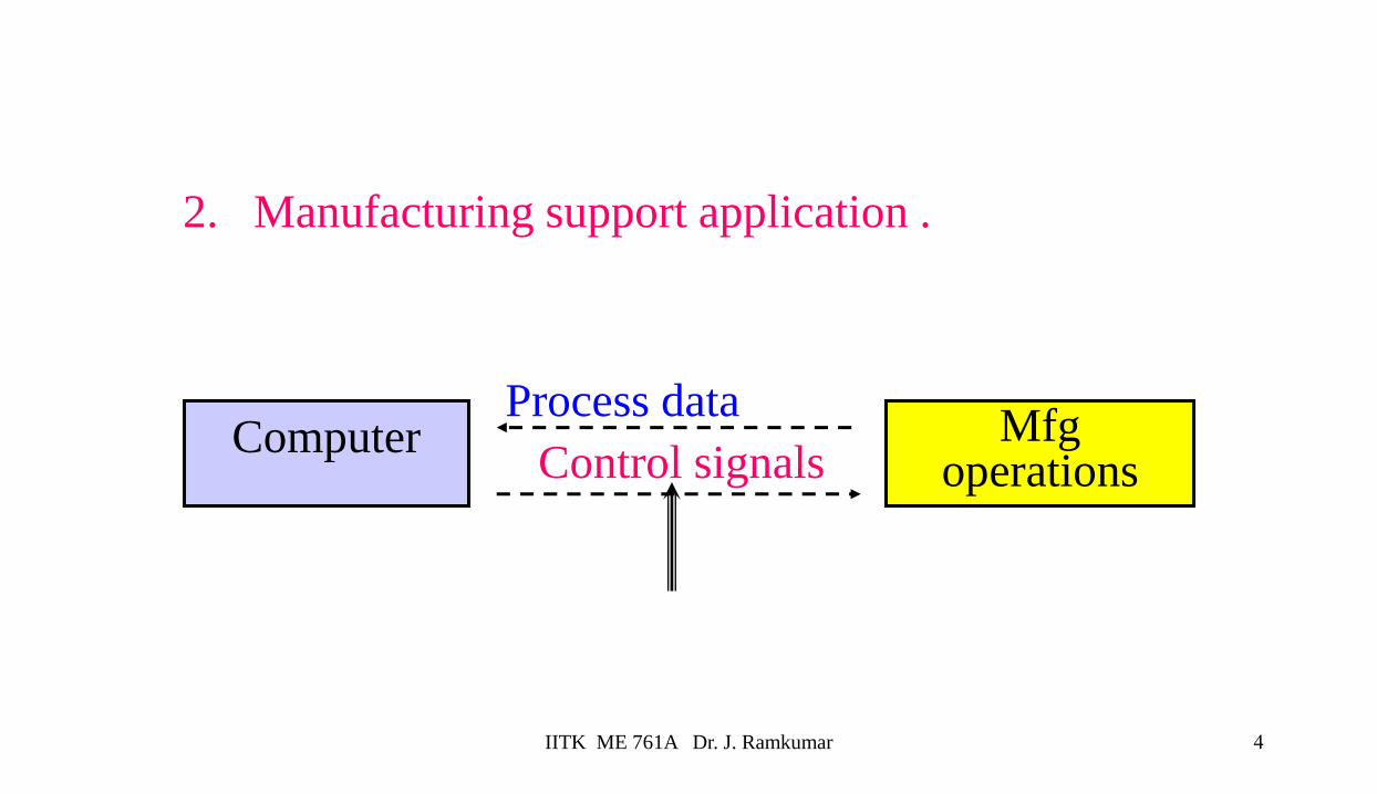
2. Manufacturing support application .
Control signalsComputer Mfg
operations
Process data
IITK ME 761A Dr. J. Ramkumar
5
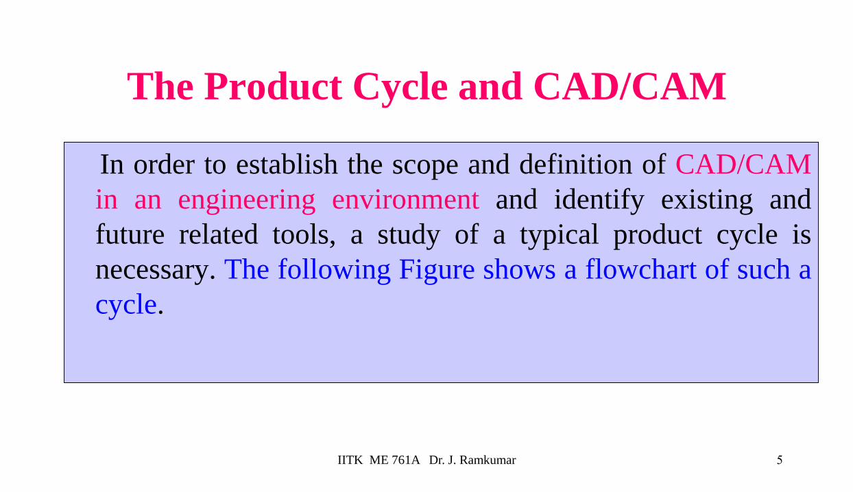
The Product Cycle and CAD/CAM
In order to establish the scope and definition of CAD/CAM
in an engineering environment and identify existing and
future related tools, a study of a typical product cycle is
necessary. The following Figure shows a flowchart of such a
cycle.
IITK ME 761A Dr. J. Ramkumar
6
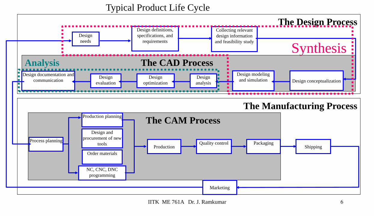
The Manufacturing Process
The Design Process
Synthesis Analysis The CAD Process
The CAM Process
Design
needs
Design definitions,
specifications, and
requirements
Collecting relevant
design information
and feasibility study
Design conceptualization
Design modeling
and simulationDesign
analysis
Design
optimization
Design
evaluation
Design documentation and
communication
Process planning
Order materials
Design and
procurement of new
tools
Production planning
NC, CNC, DNC
programming
ProductionQuality control Packaging
Marketing
Shipping
Typical Product Life Cycle
IITK ME 761A Dr. J. Ramkumar

7
• The product begins with a need which is identified based on customers'
and markets' demands.
• The product goes through two main processes from the idea
conceptualization to the finished product:
1. The design process.
2. The manufacturing process.
The main sub-processes that constitute the design process are:
1. Synthesis.
2. Analysis.
IITK ME 761A Dr. J. Ramkumar

8
Implementation of a Typical CAD Process on a
CAD/CAM system
Delineation of
geometric model
Definition translator
Geometric model
Design and
Analysis algorithms
Drafting and
detailing
Documentation
To CAM Process
Interface algorithms
Design changes
IITK ME 761A Dr. J. Ramkumar
9
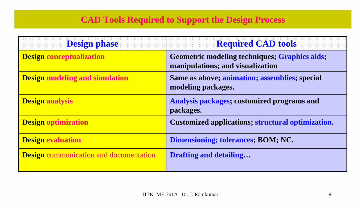
CAD Tools Required to Support the Design Process
Design phase Required CAD tools
Design conceptualization Geometric modeling techniques; Graphics aids;
manipulations; and visualization
Design modeling and simulation Same as above; animation; assemblies; special
modeling packages.
Design analysis Analysis packages; customized programs and
packages.
Design optimization Customized applications; structural optimization.
Design evaluation Dimensioning; tolerances; BOM; NC.
Design communication and documentation Drafting and detailing…
IITK ME 761A Dr. J. Ramkumar
10
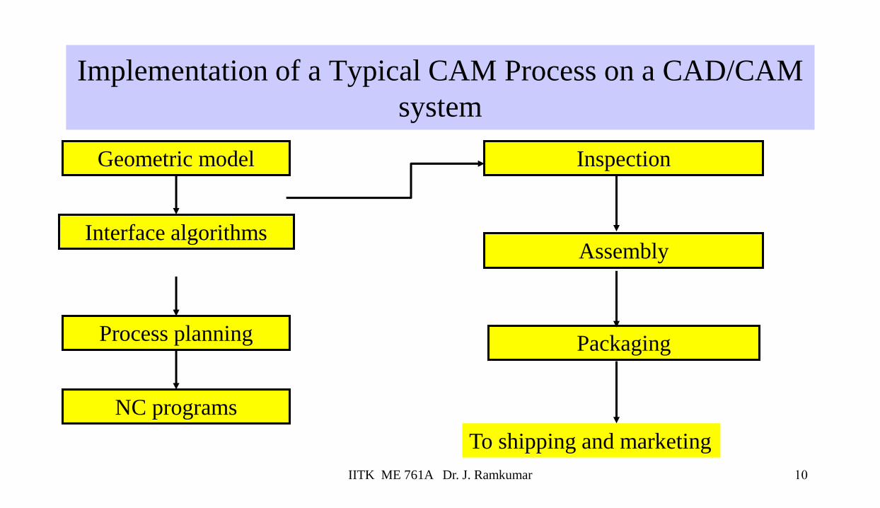
Implementation of a Typical CAM Process on a CAD/CAM
system
Geometric model
Interface algorithms
Process planning
Inspection
Assembly
Packaging
To shipping and marketing
NC programs
IITK ME 761A Dr. J. Ramkumar
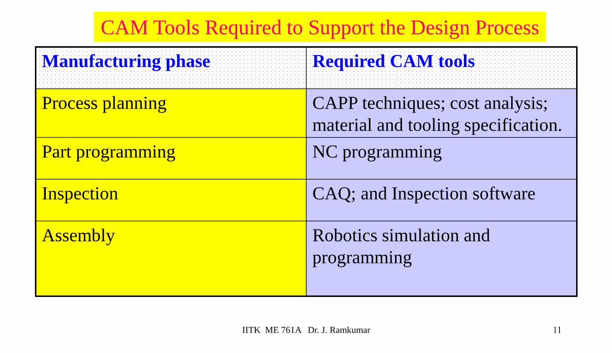
11
Manufacturing phase Required CAM tools
Process planning CAPP techniques; cost analysis;
material and tooling specification.
Part programming NC programming
Inspection CAQ; and Inspection software
Assembly Robotics simulation and
programming
CAM Tools Required to Support the Design Process
IITK ME 761A Dr. J. Ramkumar
12
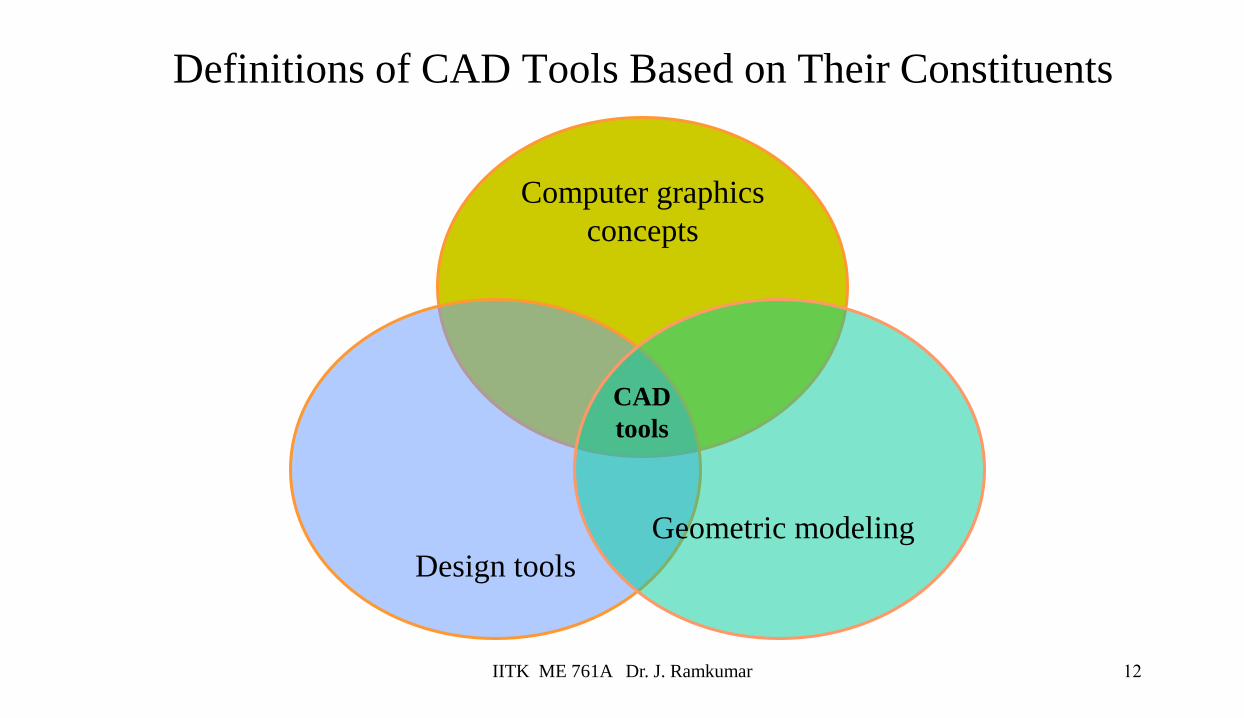
Definitions of CAD Tools Based on Their Constituents
Computer graphics
concepts
Design tools
Geometric modeling
CAD
tools
IITK ME 761A Dr. J. Ramkumar
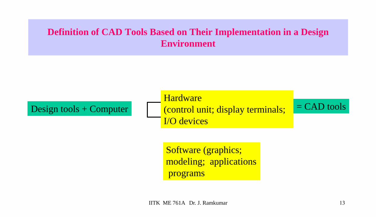
13
Definition of CAD Tools Based on Their Implementation in a Design
Environment
Design tools + Computer
Hardware
(control unit; display terminals;
I/O devices
Software (graphics;
modeling; applications
programs
= CAD tools
IITK ME 761A Dr. J. Ramkumar
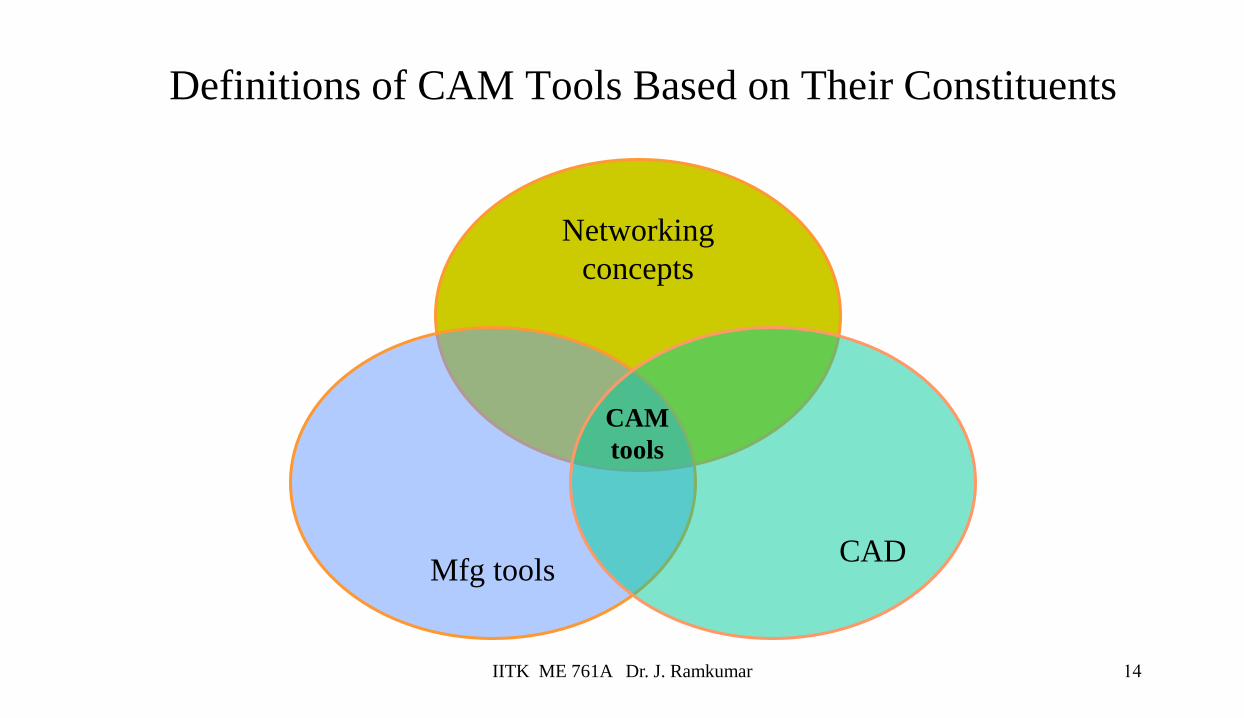
14
Definitions of CAM Tools Based on Their Constituents
Networking
concepts
Mfg toolsCAD
CAM
tools
IITK ME 761A Dr. J. Ramkumar

15
Definition of CAM Tools Based on Their Implementation in a
Manufacturing Environment
Mfg tools + Computer
Hardware
(control unit; display terminals;
I/O devices
Software (CAD; NC;
MRP; CAPP…)= CAM tools
Networking
IITK ME 761A Dr. J. Ramkumar
16
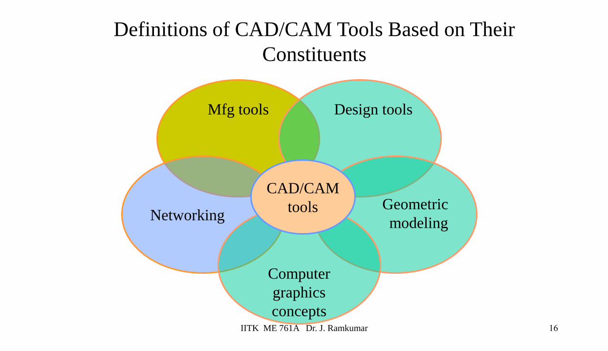
Definitions of CAD/CAM Tools Based on Their
Constituents
Mfg tools
Networking
Design tools
Geometric
modeling
Computer
graphics
concepts
CAD/CAM
tools
IITK ME 761A Dr. J. Ramkumar
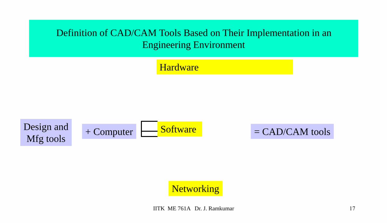
17
Definition of CAD/CAM Tools Based on Their Implementation in an
Engineering Environment
Design and
Mfg tools
Hardware
Software = CAD/CAM tools
Networking
+ Computer
IITK ME 761A Dr. J. Ramkumar

18
Geometric modeling
of conceptual design
Is design evaluation
Possible with available
Standard software?
Design testing
And evaluation
Is final design
Applicable?
Drafting
Documentation
Process planning
Are there manufacturing
discrepancies in CAD
databases?
NC programming
Machining
Inspection
Assembly
Develop customized
programs and packages
No
Yes
Yes
Yes
Geometric modeling and graphics package
Design
package
Programming
package
No
No
CAPP package
NC
package
Inspection
And Robotics
package
Typical Utilization of CAD/CAM Systems in an Industrial Environment
IITK ME 761A Dr. J. Ramkumar

19
Automation and CAD/CAM
Automation can be defined as the technology concerned
with the application of complex mechanical, electronic,
and computer-based systems in the operation and control
of manufacturing systems.
IITK ME 761A Dr. J. Ramkumar
20
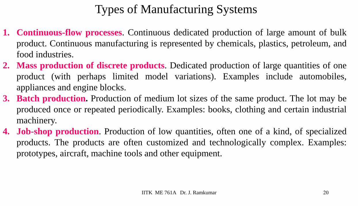
Types of Manufacturing Systems
1. Continuous-flow processes. Continuous dedicated production of large amount of bulk
product. Continuous manufacturing is represented by chemicals, plastics, petroleum, and
food industries.
2. Mass production of discrete products. Dedicated production of large quantities of one
product (with perhaps limited model variations). Examples include automobiles,
appliances and engine blocks.
3. Batch production. Production of medium lot sizes of the same product. The lot may be
produced once or repeated periodically. Examples: books, clothing and certain industrial
machinery.
4. Job-shop production. Production of low quantities, often one of a kind, of specialized
products. The products are often customized and technologically complex. Examples:
prototypes, aircraft, machine tools and other equipment.
IITK ME 761A Dr. J. Ramkumar
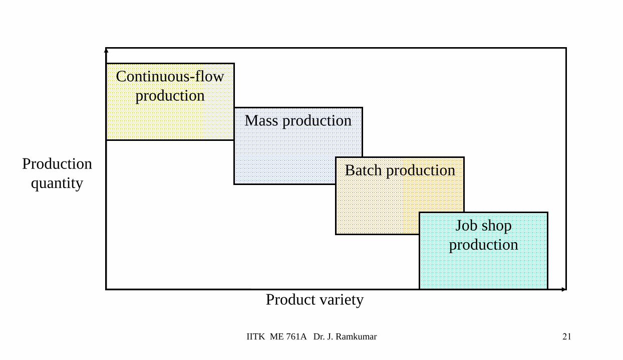
21
Production
quantity
Continuous-flow
production
Mass production
Batch production
Job shop
production
Product variety
IITK ME 761A Dr. J. Ramkumar
22
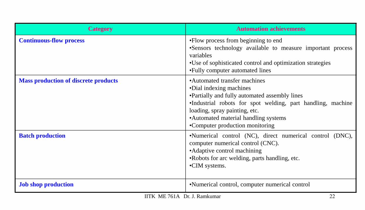
Category Automation achievements
Continuous-flow process •Flow process from beginning to end
•Sensors technology available to measure important process
variables
•Use of sophisticated control and optimization strategies
•Fully computer automated lines
Mass production of discrete products •Automated transfer machines
•Dial indexing machines
•Partially and fully automated assembly lines
•Industrial robots for spot welding, part handling, machine
loading, spray painting, etc.
•Automated material handling systems
•Computer production monitoring
Batch production •Numerical control (NC), direct numerical control (DNC),
computer numerical control (CNC).
•Adaptive control machining
•Robots for arc welding, parts handling, etc.
•CIM systems.
Job shop production •Numerical control, computer numerical control
IITK ME 761A Dr. J. Ramkumar
23
Most of the automated production systems implemented today make use of
computers. CAD/CAM in addition to its particular emphasis on the use of
computer technology, is also distinguished by the fact that it includes not only the
manufacturing operations but also the design and planning functions that precede
manufacturing.
To emphasize the differences in scope between automation and CAD/CAM,
consider the following mathematical model:
Computer Technology in Automation
IITK ME 761A Dr. J. Ramkumar
24
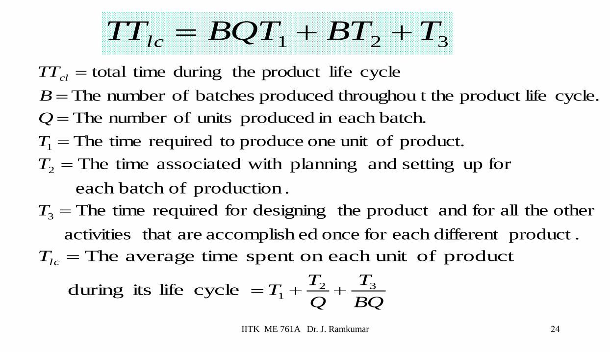
321 TBTBQTTTlc ++=
BQ
T
Q
TT
Tlc
321 cycle life its during
product ofunit each on spent timeaverage The
++=
=
.product different each for once edaccomplish are that activities
other theallfor andproduct thedesigningfor required timeThe3 =T
.production ofbatch each
for up setting and planning with associated timeThe2 =T
cycle. lifeproduct t the throughouproduced batches ofnumber The =B
product. ofunit one produce torequired timeThe1 =T
batch.each in produced units ofnumber The=Q
cycle lifeproduct theduring time total=clTT
IITK ME 761A Dr. J. Ramkumar
25
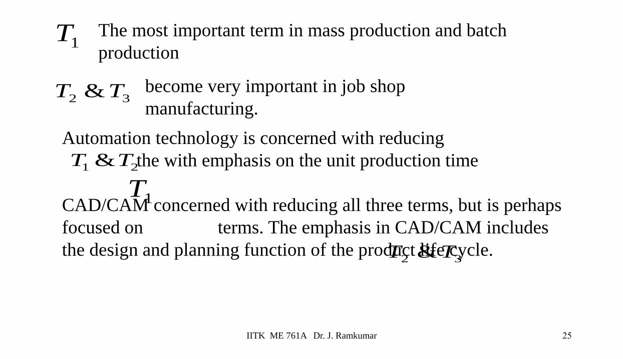
Automation technology is concerned with reducing
the with emphasis on the unit production time
CAD/CAM concerned with reducing all three terms, but is perhaps
focused on terms. The emphasis in CAD/CAM includes
the design and planning function of the product life cycle.
1T
32 &TT
The most important term in mass production and batch
production
become very important in job shop
manufacturing.
1T
32 &TT
21 &TT
IITK ME 761A Dr. J. Ramkumar
26
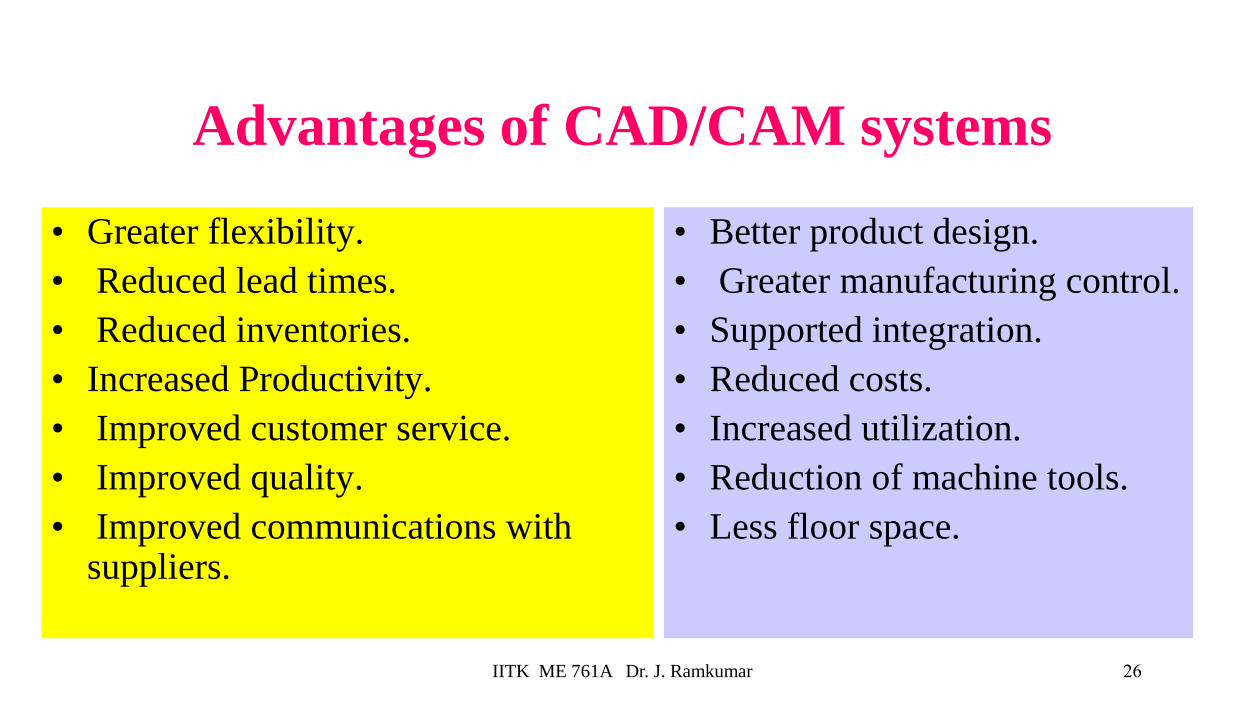
Advantages of CAD/CAM systems
• Greater flexibility.
• Reduced lead times.
• Reduced inventories.
• Increased Productivity.
• Improved customer service.
• Improved quality.
• Improved communications with suppliers.
• Better product design.
• Greater manufacturing control.
• Supported integration.
• Reduced costs.
• Increased utilization.
• Reduction of machine tools.
• Less floor space.
IITK ME 761A Dr. J. Ramkumar
27
Introduction to Geometric Transformation
• Computer graphics plays an important role in the product
development process by generating, presenting, and
manipulating geometric models of objects.
• During the product development process, for proper
understanding of designs, it is necessary not only to generate
geometric models of objects but also to perform such
manipulations on these objects as rotation, translation and
scaling.
IITK ME 761A Dr. J. Ramkumar
28
Introduction to Geometric transformation
• Essentially, computer graphics is concerned with generating, presenting and
manipulating models of an object and its different views using computer hardware,
software and graphic devices.
• Usually the numerical data generated by a computer at very high speeds is hard to
interpret unless one represents the data in graphic format and it is even better if the
graphic can be manipulated to be viewed from different sides, enlarged or reduced
in size.
• Geometric transformation is one of the basic techniques that is used to accomplish
these graphic functions involving scale change, translation to another location or
rotating it by a certain angle to get a better view of it.
IITK ME 761A Dr. J. Ramkumar
29
2D Transformations
IITK ME 761A Dr. J. Ramkumar

30
Rotation About the OriginTo rotate a line or polygon, we must rotate each of
its vertices.
To rotate point (x1,y1) to point (x2,y2) we observe:
From the illustration we know that:
sin (A + B) = y2/r cos (A + B) = x2/r
sin A = y1/r cos A = x1/r
x-axis
(x1,y1)
(x2,y2)
A
Br
(0,0)
y-axis
IITK ME 761A Dr. J. Ramkumar

31
Rotation About the Origin
From the double angle formulas: sin (A + B) = sinAcosB + cosAsinB
cos (A + B)= cosAcosB - sinAsinB
Substituting: y2/r = (y1/r)cosB + (x1/r)sinB
Therefore: y2 = y1cosB + x1sinB
We have x2 = x1cosB - y1sinB
y2 = x1sinB + y1cosB
P2 = R P1.
(x1)
(y1)
(cosB -sinB)
(sinB cosB)
(x2)
(y2) =
IITK ME 761A Dr. J. Ramkumar
32
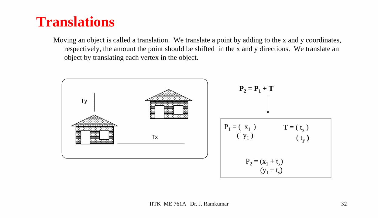
TranslationsMoving an object is called a translation. We translate a point by adding to the x and y coordinates,
respectively, the amount the point should be shifted in the x and y directions. We translate an
object by translating each vertex in the object.
P2 = P1 + T
T = ( tx )
( ty )
P1 = ( x1 )
( y1 )
P2 = (x1 + tx)
(y1 + ty)
Ty
Tx
IITK ME 761A Dr. J. Ramkumar

33
Scaling
Changing the size of an object is called a scale. We scale an object by scaling the x and y coordinates
of each vertex in the object.
P2 = S P1
.
S = (sx 0)
(0 sy)P1 = ( x1 )
( y1 )
P2 = (sxx1)
(syy1)
IITK ME 761A Dr. J. Ramkumar
34
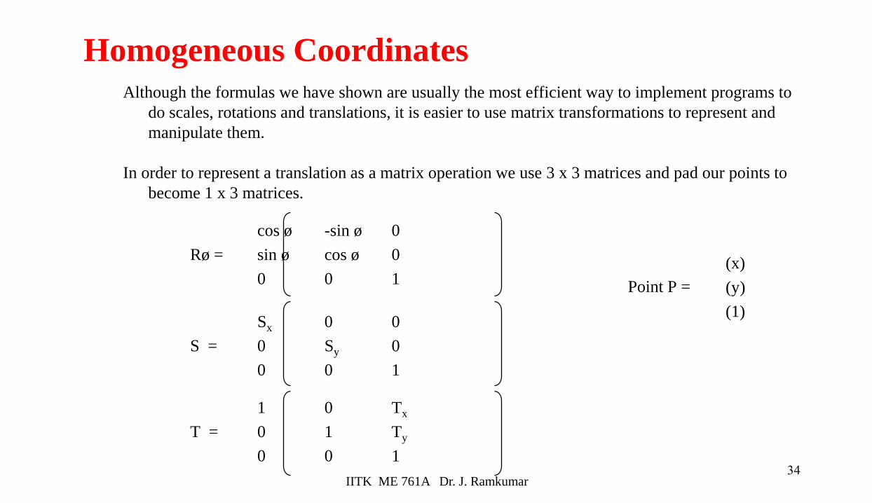
Homogeneous CoordinatesAlthough the formulas we have shown are usually the most efficient way to implement programs to
do scales, rotations and translations, it is easier to use matrix transformations to represent and
manipulate them.
In order to represent a translation as a matrix operation we use 3 x 3 matrices and pad our points to
become 1 x 3 matrices.
cos ø -sin ø 0
Rø = sin ø cos ø 0
0 0 1
Sx 0 0
S = 0 Sy 0
0 0 1
1 0 Tx
T = 0 1 Ty
0 0 1
Point P =
(x)
(y)
(1)
IITK ME 761A Dr. J. Ramkumar
35
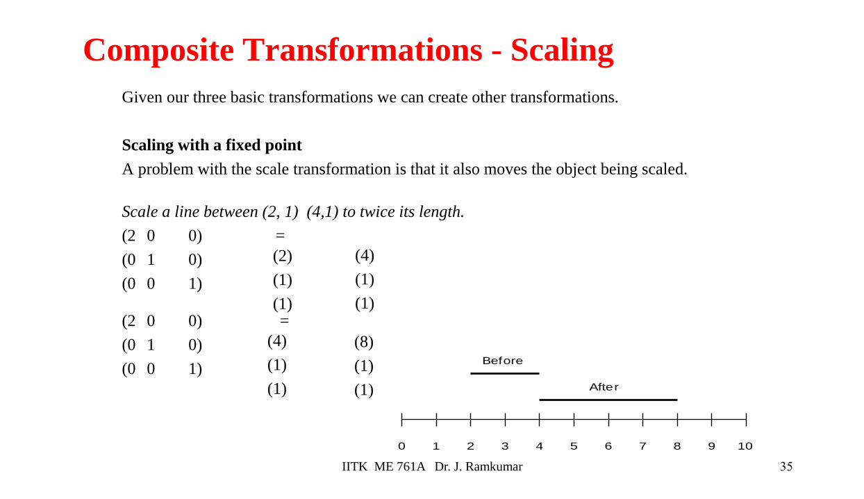
Composite Transformations - Scaling
Given our three basic transformations we can create other transformations.
Scaling with a fixed point
A problem with the scale transformation is that it also moves the object being scaled.
Scale a line between (2, 1) (4,1) to twice its length.
(2 0 0) =
(0 1 0)
(0 0 1)
(2 0 0) =
(0 1 0)
(0 0 1)
0 1 2 3 4 5 6 7 8 9 10
Before
After
(2)
(1)
(1)
(4)
(1)
(1)
(4)
(1)
(1)
(8)
(1)
(1)
IITK ME 761A Dr. J. Ramkumar
36
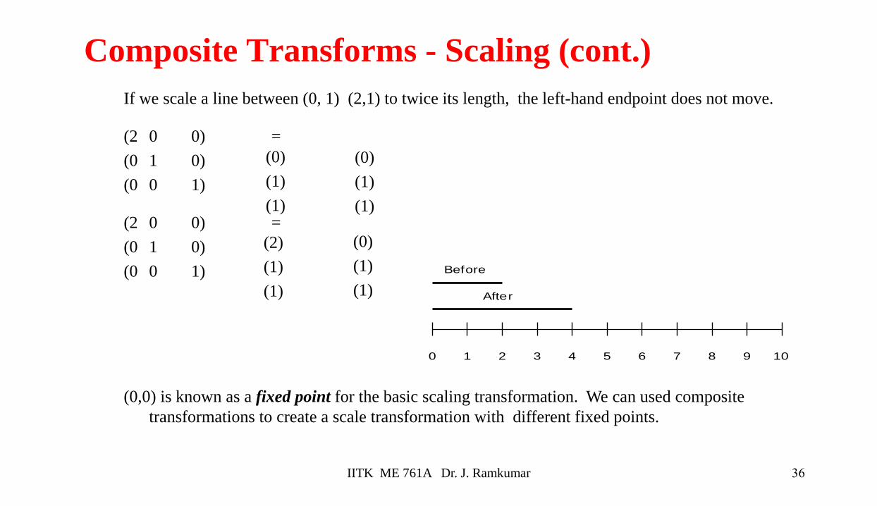
Composite Transforms - Scaling (cont.)
If we scale a line between (0, 1) (2,1) to twice its length, the left-hand endpoint does not move.
(2 0 0) =
(0 1 0)
(0 0 1)
(2 0 0) =
(0 1 0)
(0 0 1)
(0,0) is known as a fixed point for the basic scaling transformation. We can used composite
transformations to create a scale transformation with different fixed points.
0 1 2 3 4 5 6 7 8 9 10
Before
After
(0)
(1)
(1)
(0)
(1)
(1)
(2)
(1)
(1)
(0)
(1)
(1)
IITK ME 761A Dr. J. Ramkumar
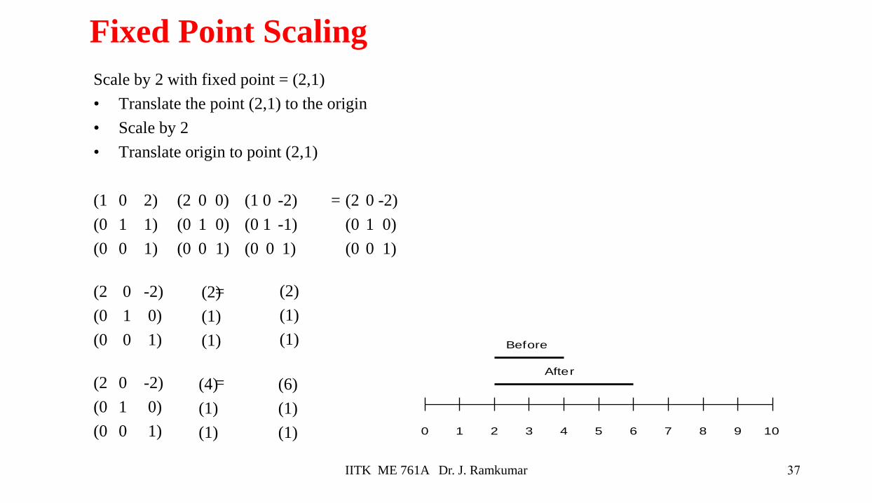
37
Fixed Point Scaling
Scale by 2 with fixed point = (2,1)
• Translate the point (2,1) to the origin
• Scale by 2
• Translate origin to point (2,1)
(1 0 2) (2 0 0) (1 0 -2) = (2 0 -2)
(0 1 1) (0 1 0) (0 1 -1) (0 1 0)
(0 0 1) (0 0 1) (0 0 1) (0 0 1)
(2 0 -2) =
(0 1 0)
(0 0 1)
(2 0 -2) =
(0 1 0)
(0 0 1) 0 1 2 3 4 5 6 7 8 9 10
Before
After
(2)
(1)
(1)
(2)
(1)
(1)
(4)
(1)
(1)
(6)
(1)
(1)
IITK ME 761A Dr. J. Ramkumar
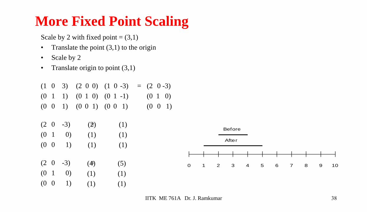
38
More Fixed Point ScalingScale by 2 with fixed point = (3,1)
• Translate the point (3,1) to the origin
• Scale by 2
• Translate origin to point (3,1)
(1 0 3) (2 0 0) (1 0 -3) = (2 0 -3)
(0 1 1) (0 1 0) (0 1 -1) (0 1 0)
(0 0 1) (0 0 1) (0 0 1) (0 0 1)
(2 0 -3) =
(0 1 0)
(0 0 1)
(2 0 -3) =
(0 1 0)
(0 0 1)
0 1 2 3 4 5 6 7 8 9 10
Before
After
(2)
(1)
(1)
(1)
(1)
(1)
(4)
(1)
(1)
(5)
(1)
(1)
IITK ME 761A Dr. J. Ramkumar
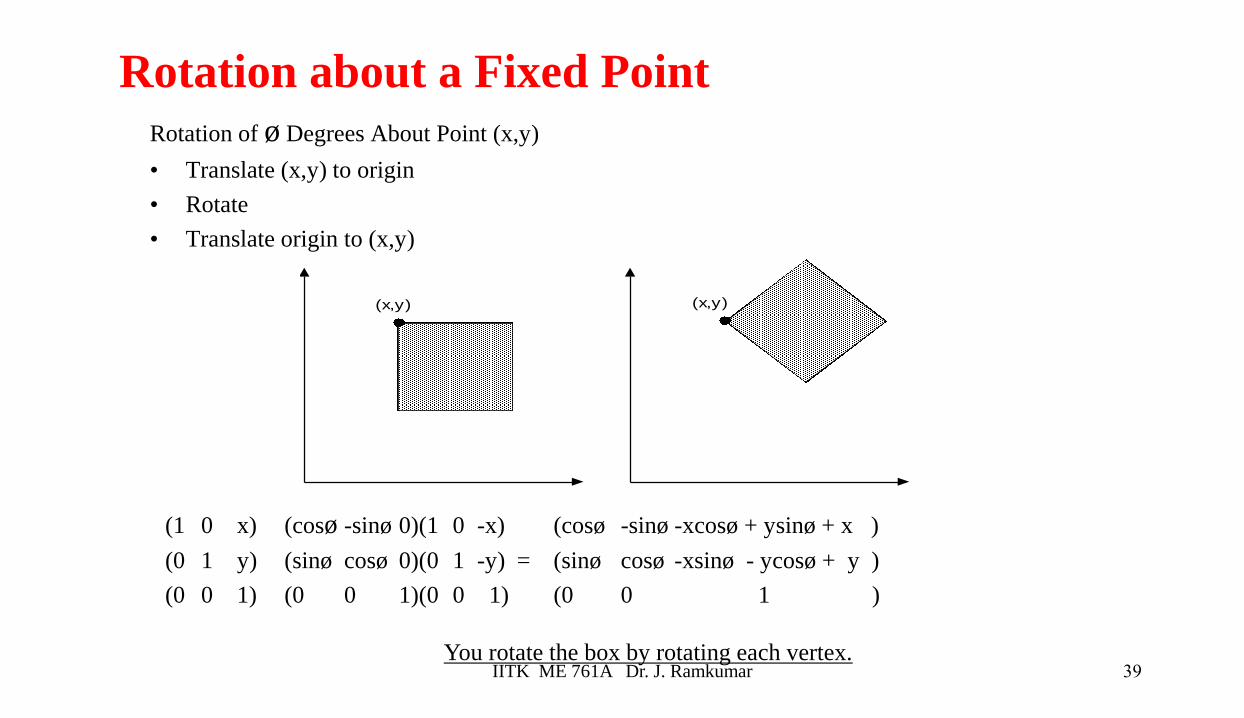
39
Rotation about a Fixed Point
Rotation of ø Degrees About Point (x,y)
• Translate (x,y) to origin
• Rotate
• Translate origin to (x,y)
(1 0 x) (cosø -sinø 0)(1 0 -x) (cosø -sinø -xcosø + ysinø + x )
(0 1 y) (sinø cosø 0)(0 1 -y) = (sinø cosø -xsinø - ycosø + y )
(0 0 1) (0 0 1)(0 0 1) (0 0 1 )
You rotate the box by rotating each vertex.
(x,y) (x,y)
IITK ME 761A Dr. J. Ramkumar
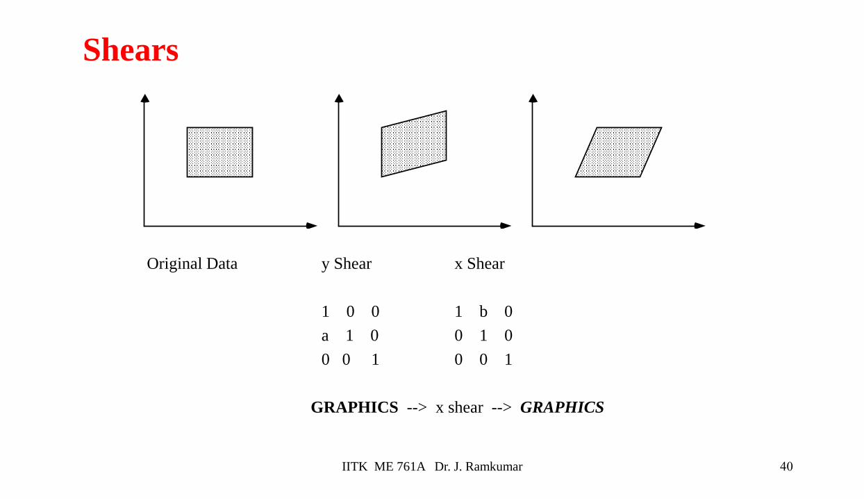
40
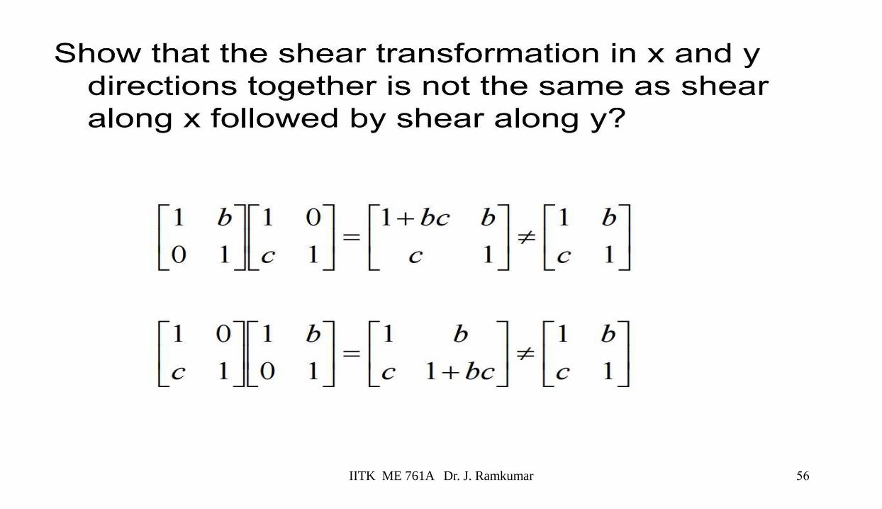
Shears
Original Data y Shear x Shear
1 0 0 1 b 0
a 1 0 0 1 0
0 0 1 0 0 1
GRAPHICS --> x shear --> GRAPHICS
IITK ME 761A Dr. J. Ramkumar

41
Reflections
Reflection about the y-axis Reflection about the x-axis
-1 0 0 1 0 0
0 1 0 0 -1 0
0 0 1 0 0 1
IITK ME 761A Dr. J. Ramkumar

42
More Reflections
Reflection about the origin Reflection about the line y=x
-1 0 0 0 1 0
0 -1 0 1 0 0
0 0 1 0 0 1
IITK ME 761A Dr. J. Ramkumar
IITK ME 761A Dr. J. Ramkumar43
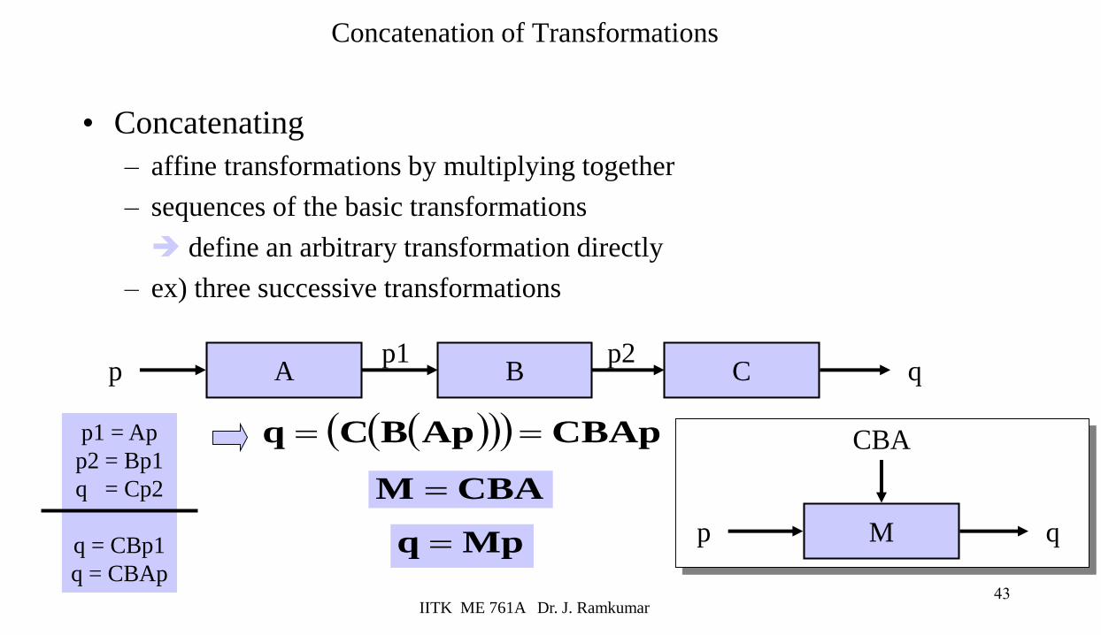
Concatenation of Transformations
• Concatenating
– affine transformations by multiplying together
– sequences of the basic transformations
➔ define an arbitrary transformation directly
– ex) three successive transformations
( )( )( ) CBApApBCq ==
A B Cp q
CBAM =
Mpq = Mp q
CBAp1 = Ap
p2 = Bp1
q = Cp2
q = CBp1
q = CBAp
p1 p2
IITK ME 761A Dr. J. Ramkumar 44
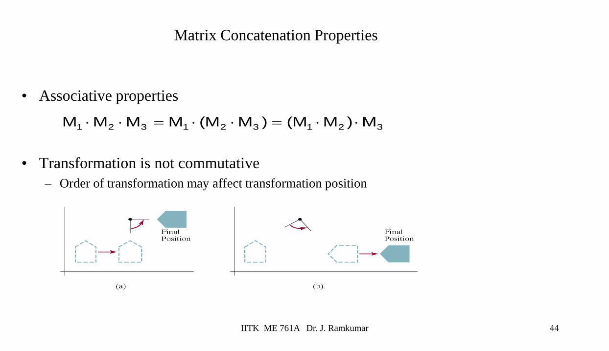
Matrix Concatenation Properties
• Associative properties
• Transformation is not commutative
– Order of transformation may affect transformation position
321321321 M)MM()MM(MMMM ==

IITK ME 761A Dr. J. Ramkumar 45
Two-dimensional composite transformation (1)
• Composite transformation
– A sequence of transformations
– Calculate composite transformation matrix rather than applying individual transformations
• Composite two-dimensional translations
– Apply two successive translations, T1 and T2
– Composite transformation matrix in coordinate form
PM'P
PMM'P 12
=
=
PTTPTTP
ttTT
ttTT
yx
yx
==
=
=
)()('
),(
),(
1212
222
111
)tt,tt(T)t,t(T)t,t(T y2y1x2x1y1x1y2x2 ++=

IITK ME 761A Dr. J. Ramkumar 46
Two-dimensional composite transformation (2)
• Composite two-dimensional rotations
– Two successive rotations, R1 and R2 into a point P
– Multiply two rotation matrices to get composite transformation matrix
• Composite two-dimensional scaling
P)}(R)(R{'P
}P)(R{)(R'P
21
21
=
=
P)ss,ss(S'P
)ss,ss(S)s,s(S)s,s(S
y2y1x2x1
y2y1x2x1y2x2y1x1
=
=
P)(R'P
)(R)(R)(R
21
2121
+=
+=

IITK ME 761A Dr. J. Ramkumar 47
Two-dimensional composite transformation (3)
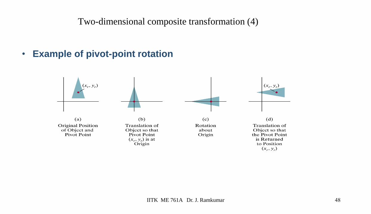
• General two-dimensional Pivot-point rotation
– Graphics package provide only origin rotation
– Perform a translate-rotate-translate sequence• Translate the object to move pivot-point position to origin
• Rotate the object
• Translate the object back to the original position
– Composite matrix in coordinates form ),y,x(R)y,x(T)(R)y,x(T rrrrrr =−−
IITK ME 761A Dr. J. Ramkumar 48
Two-dimensional composite transformation (4)
• Example of pivot-point rotation
IITK ME 761A Dr. J. Ramkumar 49
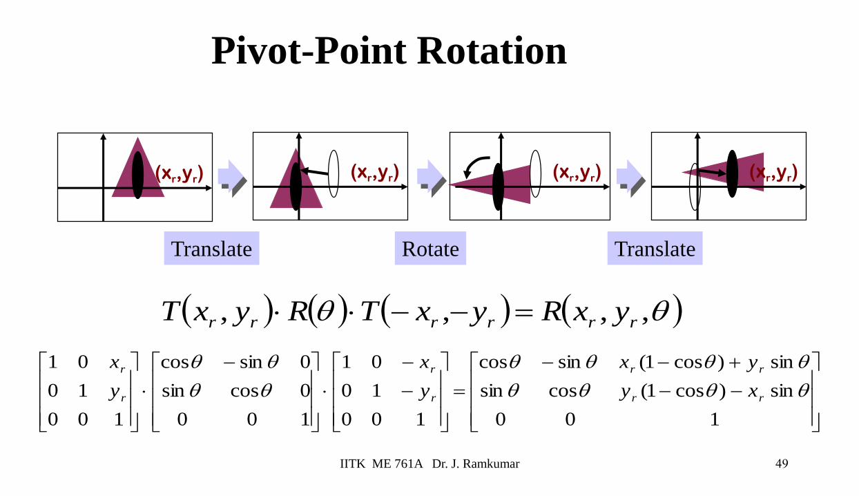
Pivot-Point Rotation
−−
+−−
=
−
−
−
100
sin)cos1(cossin
sin)cos1(sincos
100
10
01
100
0cossin
0sincos
100
10
01
rr
rr
r
r
r
r
xy
yx
y
x
y
x
( ) ( ) ( ) ( ) ,,,, rrrrrr yxRyxTRyxT =−−
Translate Rotate Translate
(xr,yr) (xr,yr) (xr,yr)(xr,yr)
IITK ME 761A Dr. J. Ramkumar 50
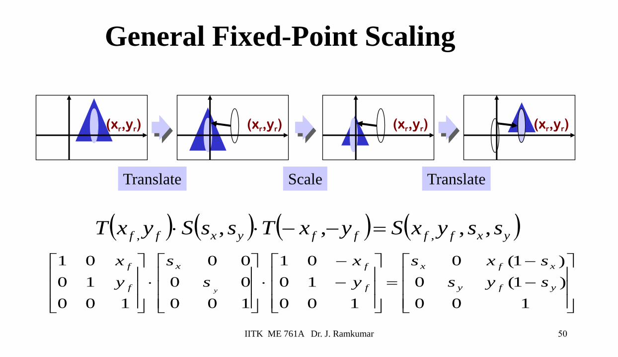
General Fixed-Point Scaling
−
−
=
−
−
100
)1(0
)1(0
100
10
01
100
00
00
100
10
01
yfy
xfx
f
fx
f
f
sys
sxs
y
x
s
s
y
x
y
Translate Scale Translate
(xr,yr) (xr,yr) (xr,yr) (xr,yr)
( ) ( ) ( ) ( )yxffffyxff ssyxSyxTssSyxT ,,,, ,, =−−
IITK ME 761A Dr. J. Ramkumar 51
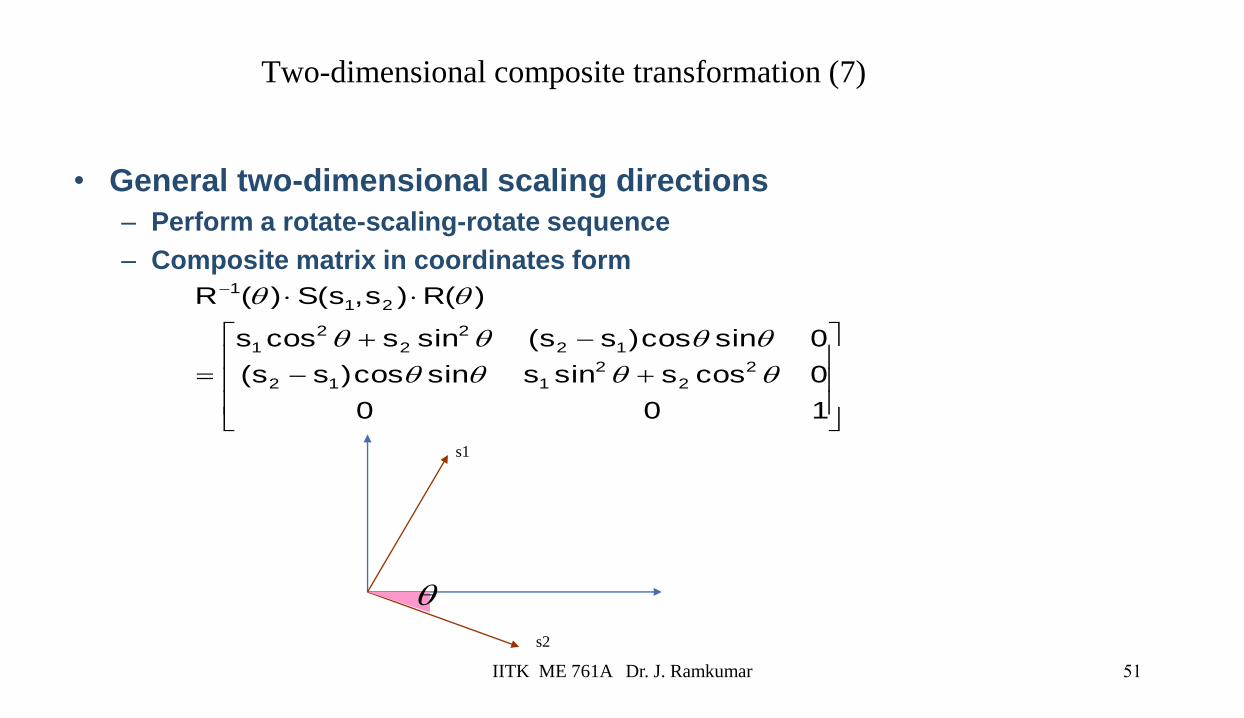
Two-dimensional composite transformation (7)
• General two-dimensional scaling directions
– Perform a rotate-scaling-rotate sequence
– Composite matrix in coordinates form
+−
−+
=
−
100
0cosssinssincos)ss(
0sincos)ss(sinscoss
)(R)s,s(S)(R
22
2112
122
22
1
211
s1
s2
IITK ME 761A Dr. J. Ramkumar 52
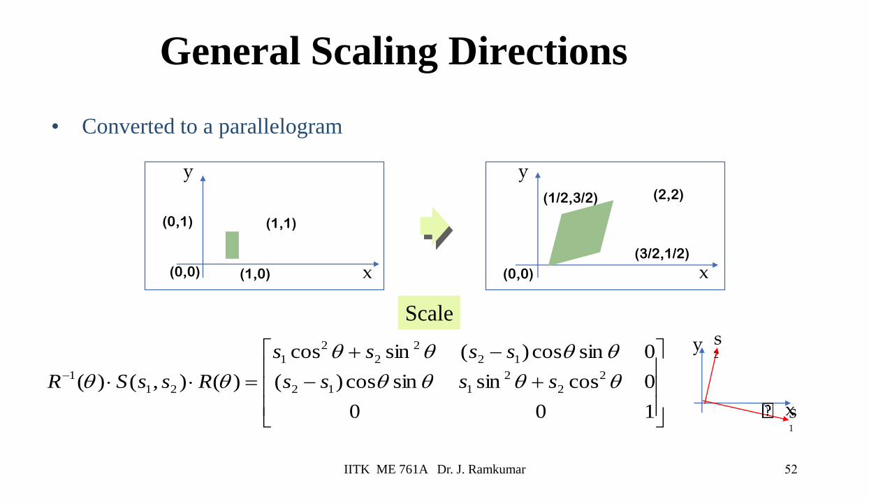
General Scaling Directions
• Converted to a parallelogram
+−
−+
=−
100
0cossinsincos)(
0sincos)(sincos
)(),()( 2
2
2
112
12
2
2
2
1
21
1
ssss
ssss
RssSR
x
y
(0,0)
(3/2,1/2)
(1/2,3/2) (2,2)
x
y
(0,0) (1,0)
(0,1) (1,1)
x
y s2
s1
Scale

IITK ME 761A Dr. J. Ramkumar53
General Rotation (1/2)
• Three successive rotations about the three axes
rotation of a cube about the z axis rotation of a cube about the y axis
rotation of a cube about the x axis
?
IITK ME 761A Dr. J. Ramkumar 54
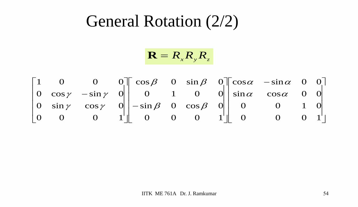
General Rotation (2/2)
zyxRRR=R
−
−
−
1000
0100
00cossin
00sincos
1000
0cos0sin
0010
0sin0cos
1000
0cossin0
0sincos0
0001
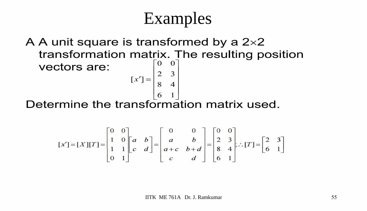
Examples
IITK ME 761A Dr. J. Ramkumar 55
IITK ME 761A Dr. J. Ramkumar 56
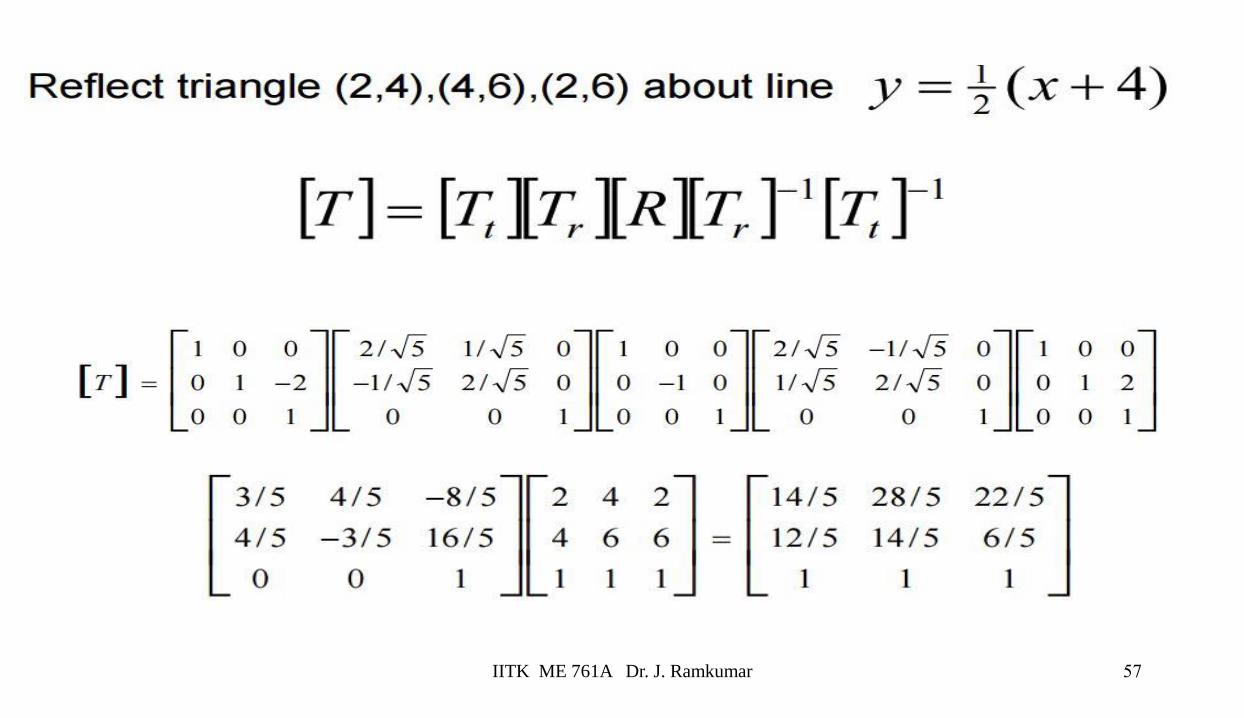
IITK ME 761A Dr. J. Ramkumar 57

3D Transformation
◼ A 3D point (x,y,z) – x,y, and z coordinates
◼ We will still use column vectors to represent points
◼ Homogeneous coordinates of a 3D point
(x,y,z,1)
◼ Transformation will be performed using 4x4 matrix
x
y
z
58
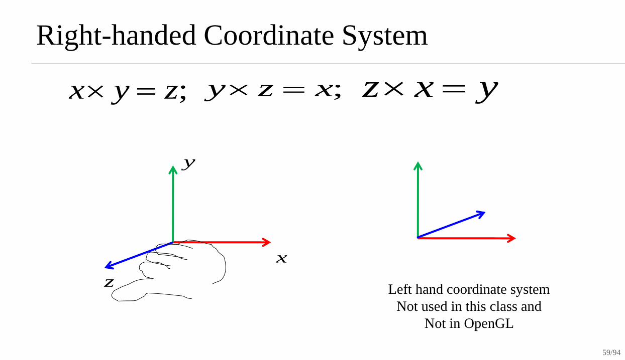
Right-handed Coordinate System
x
y
z
;zyx = ;xzy = yxz =
Left hand coordinate system
Not used in this class and
Not in OpenGL
59/94
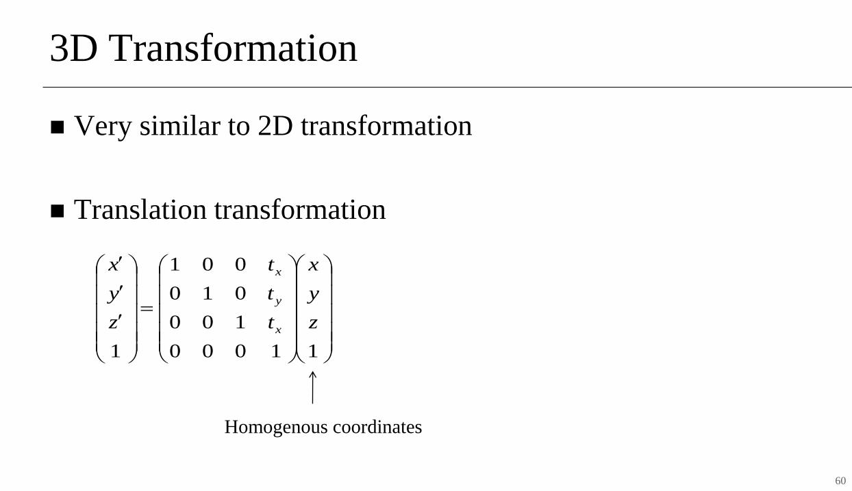
3D Transformation
◼ Very similar to 2D transformation
◼ Translation transformation
=
11000
100
010
001
1
z
y
x
t
t
t
z
y
x
x
y
x
Homogenous coordinates
60
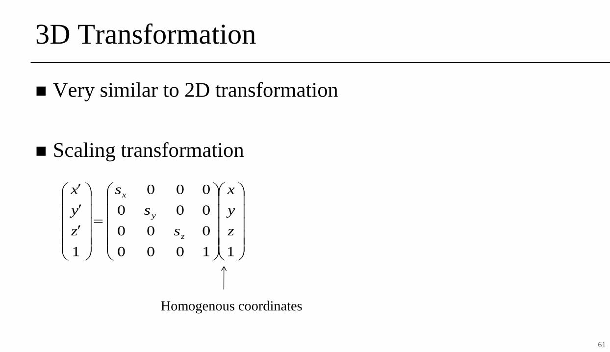
3D Transformation
◼ Very similar to 2D transformation
◼ Scaling transformation
=
11000
000
000
000
1
z
y
x
s
s
s
z
y
x
z
y
x
Homogenous coordinates
61

3D Transformation
◼ 3D rotation is done around a rotation axis
◼ Fundamental rotations – rotate about x, y, or z axes
◼ Counter-clockwise rotation is referred to as positive rotation
(when you look down negative axis)
x
y
z
+
62
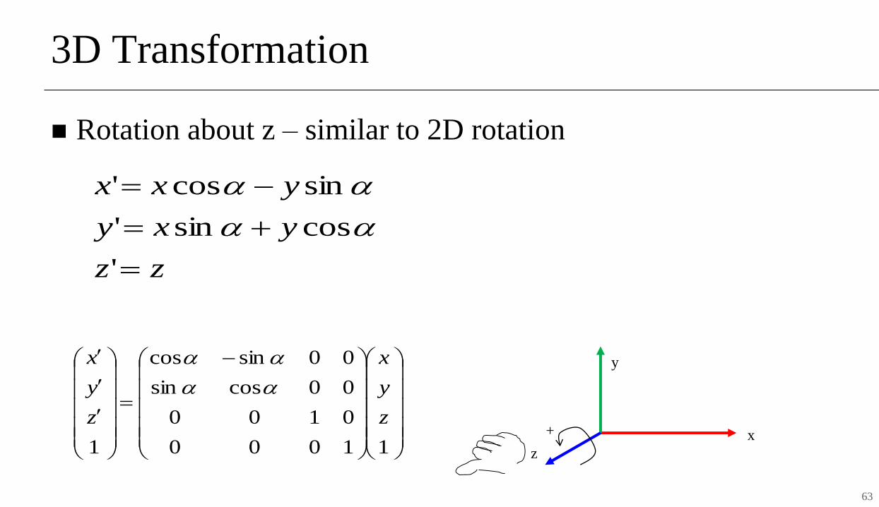
3D Transformation
◼ Rotation about z – similar to 2D rotation
x
y
z
+
−
=
11000
0100
00cossin
00sincos
1
z
y
x
z
y
x
zz
yxy
yxx
=
+=
−=
'
cossin'
sincos'
63
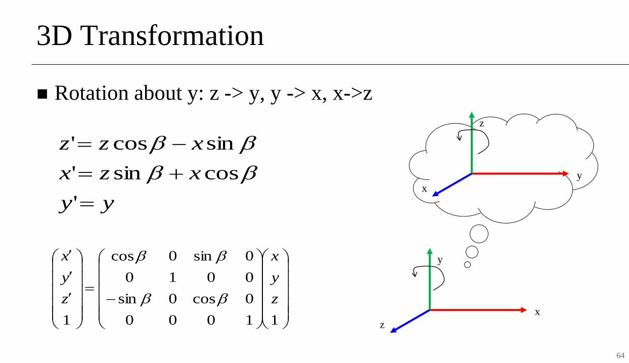
3D Transformation
◼ Rotation about y: z -> y, y -> x, x->z
−=
11000
0cos0sin
0010
0sin0cos
1
z
y
x
z
y
x
yy
xzx
xzz
=
+=
−=
'
cossin'
sincos'
y
z
x
x
y
z
64
3D Transformation
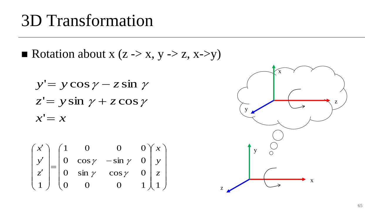
◼ Rotation about x (z -> x, y -> z, x->y)
x
y
z
−=
11000
0cossin0
0sincos0
0001
1
z
y
x
z
y
x
xx
zyz
zyy
=
+=
−=
'
cossin'
sincos'
z
x
y
65
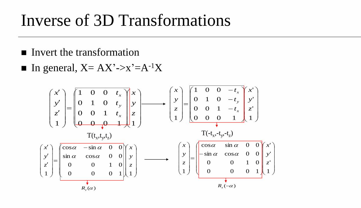
Inverse of 3D Transformations
◼ Invert the transformation
◼ In general, X= AX’->x’=A-1X
=
11000
100
010
001
1
z
y
x
t
t
t
z
y
x
x
y
x
−
−
−
=
1
'
'
'
1000
100
010
001
1
z
y
x
t
t
t
z
y
x
x
y
x
−
=
11000
0100
00cossin
00sincos
1
z
y
x
z
y
x
−=
1
'
'
'
1000
0100
00cossin
00sincos
1
z
y
x
z
y
x
)(zR)( −zR
T(tx,ty,tz)T(-tx,-ty,-tz)

3D Rotation about Arbitrary Axes
◼ Rotate p about the by the angle
x
y
zr
),,( zyxp =
r
67
3-D Rotation
◼ General rotations in 3-D require rotating about an arbitrary axis of rotation
◼ Deriving the rotation matrix for such a rotation directly is a good exercise in linear algebra
◼ The general rotation matrix is a combination of coordinate-axis rotations and translations!
68
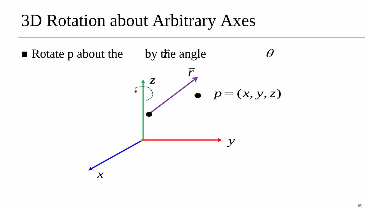
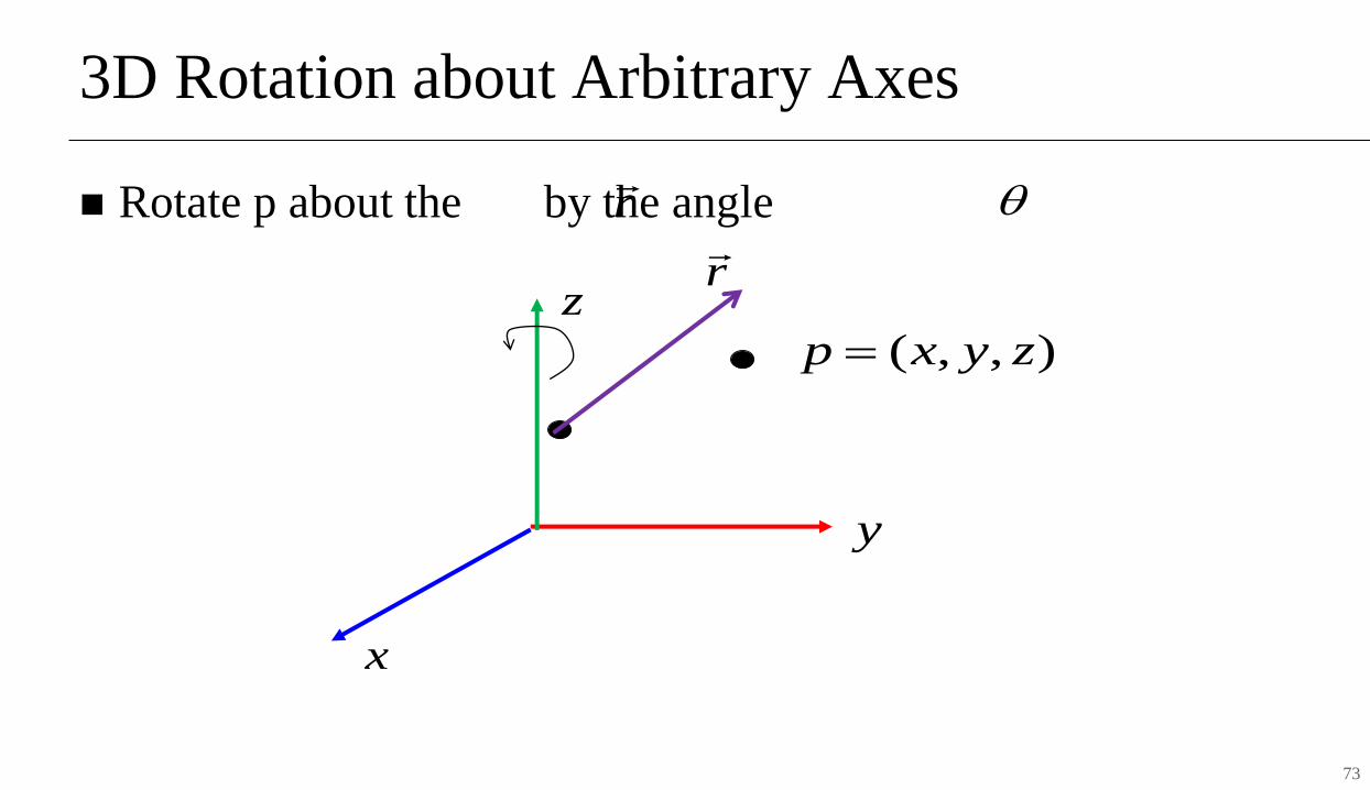
3D Rotation about Arbitrary Axes
◼ Rotate p about the by the angle
x
y
zr
),,( zyxp =
r
69
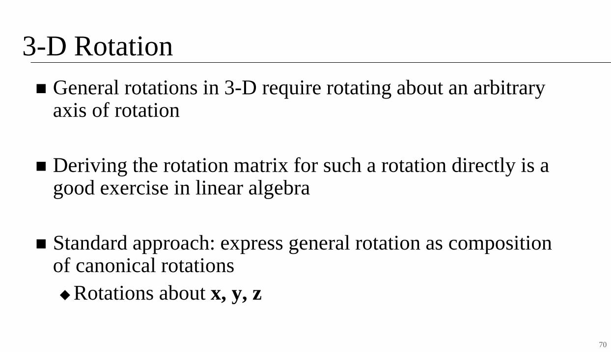
3-D Rotation
◼ General rotations in 3-D require rotating about an arbitrary axis of rotation
◼ Deriving the rotation matrix for such a rotation directly is a good exercise in linear algebra
◼ Standard approach: express general rotation as composition of canonical rotations
◆Rotations about x, y, z
70
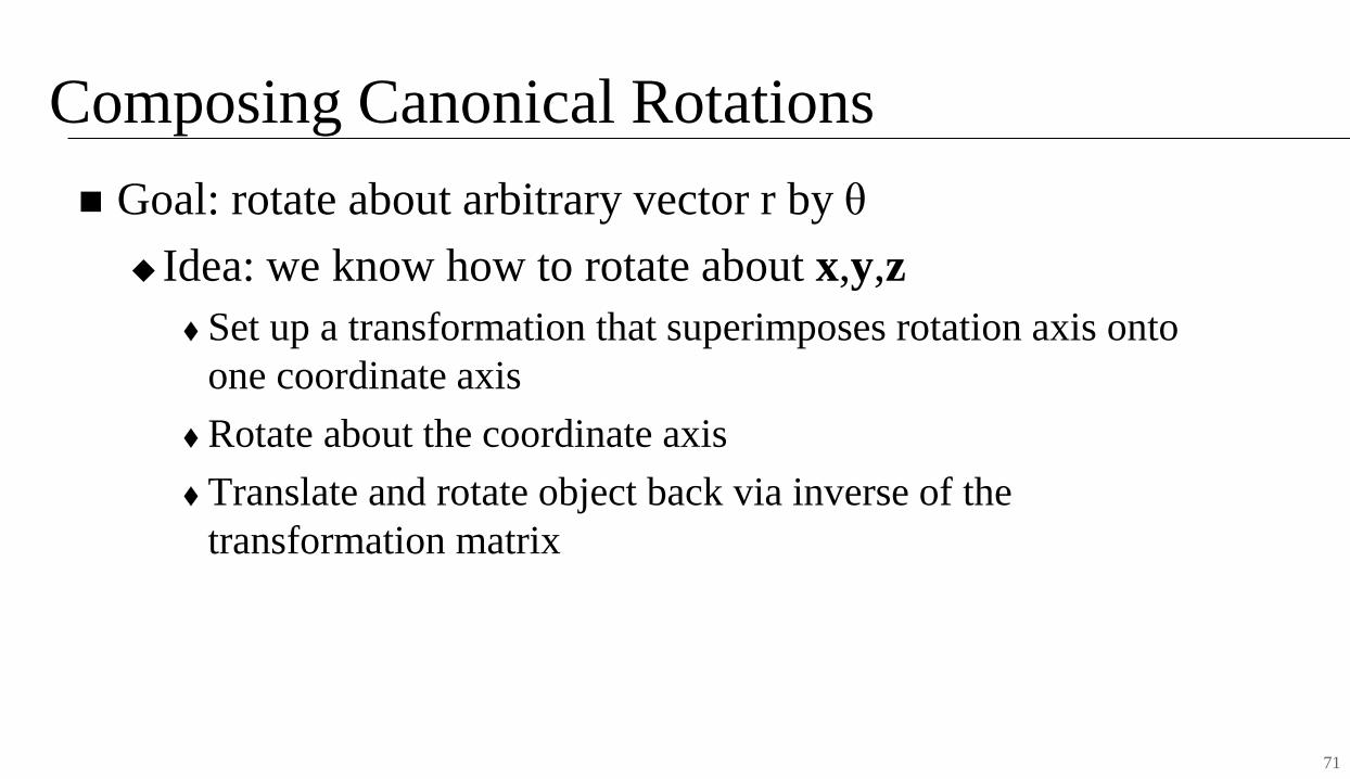
Composing Canonical Rotations
◼ Goal: rotate about arbitrary vector r by θ
◆ Idea: we know how to rotate about x,y,z
⧫ Set up a transformation that superimposes rotation axis onto
one coordinate axis
⧫ Rotate about the coordinate axis
⧫ Translate and rotate object back via inverse of the
transformation matrix
71
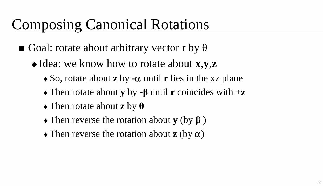
Composing Canonical Rotations
◼ Goal: rotate about arbitrary vector r by θ
◆ Idea: we know how to rotate about x,y,z
⧫ So, rotate about z by - until r lies in the xz plane
⧫ Then rotate about y by -β until r coincides with +z
⧫ Then rotate about z by θ
⧫ Then reverse the rotation about y (by β )
⧫ Then reverse the rotation about z (by )
72
3D Rotation about Arbitrary Axes
◼ Rotate p about the by the angle
x
y
zr
),,( zyxp =
r
73
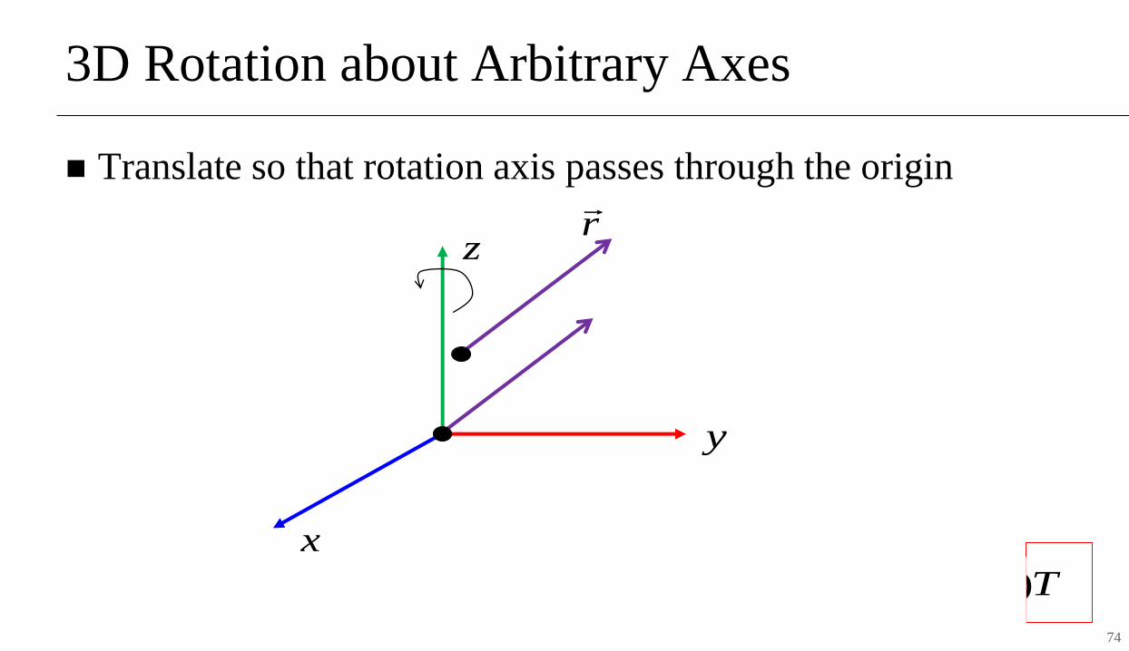
3D Rotation about Arbitrary Axes
◼ Translate so that rotation axis passes through the origin
x
y
zr
TRRRRRT zyzyz )()()()()(1 −−−
74
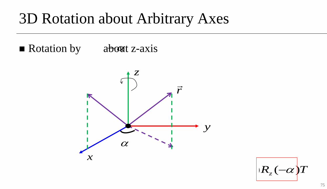
3D Rotation about Arbitrary Axes
◼ Rotation by about z-axis
x
y
z
−
r
TRRRRRT zyzyy )()()()()(1 −−−
75
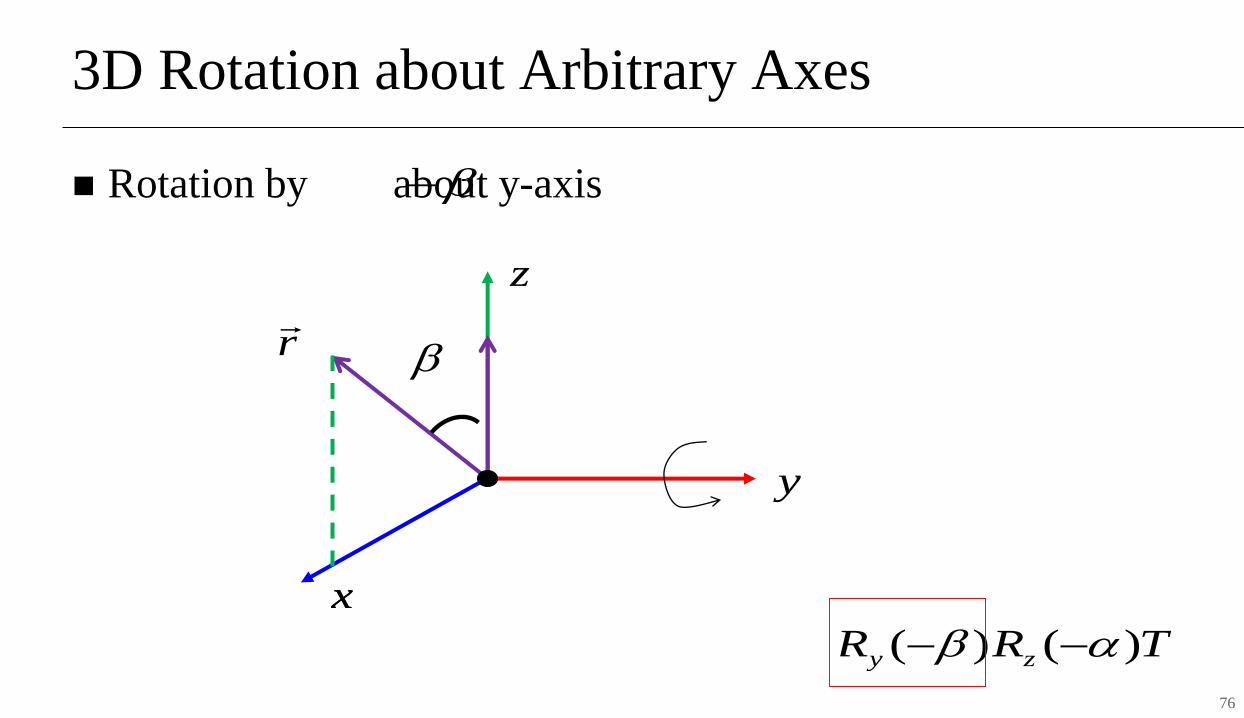
3D Rotation about Arbitrary Axes
◼ Rotation by about y-axis
x
y
z
−
r
x
TRRRRRT zyzyy )()()()()(1 −−−
76
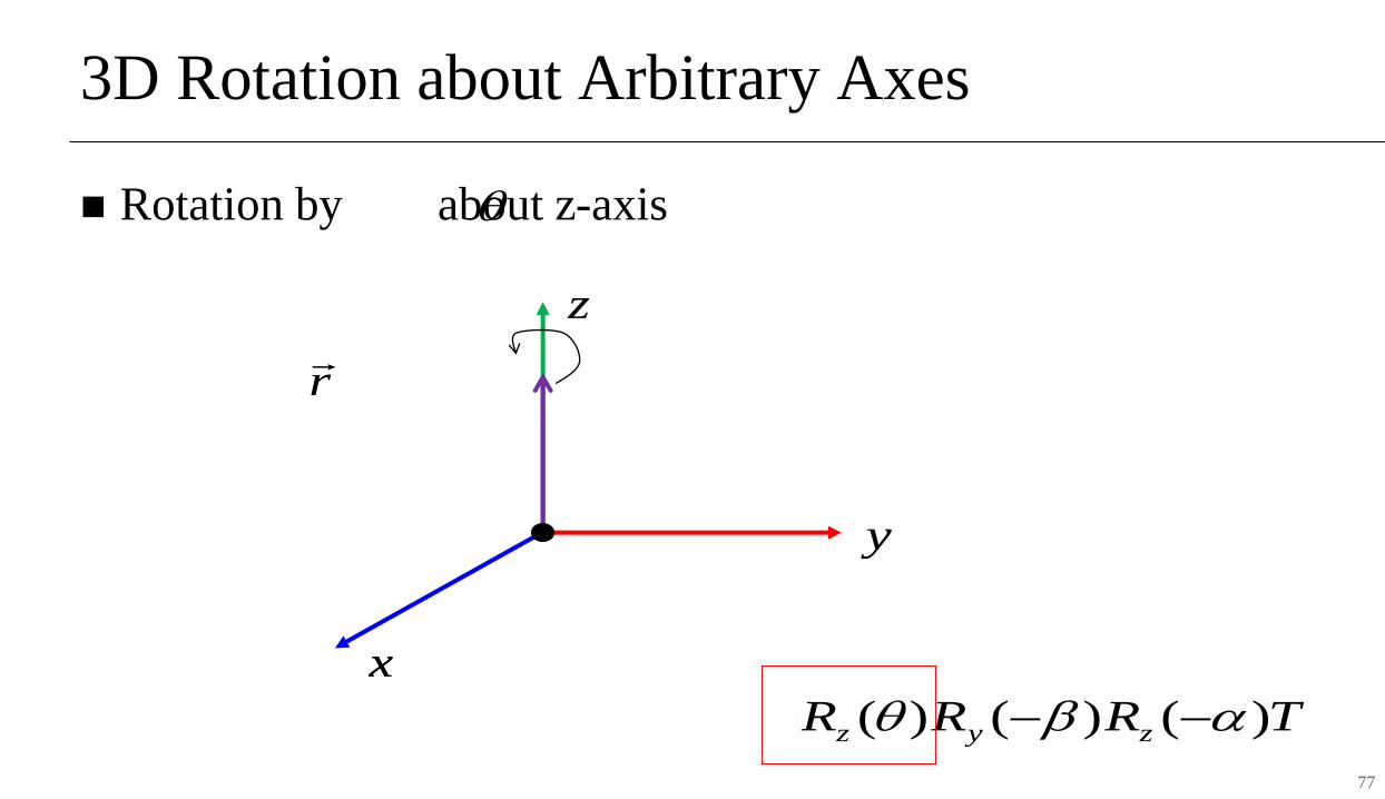
3D Rotation about Arbitrary Axes
◼ Rotation by about z-axis
x
y
z
r
x
TRRRRRT zyzyy )()()()()(1 −−−
77
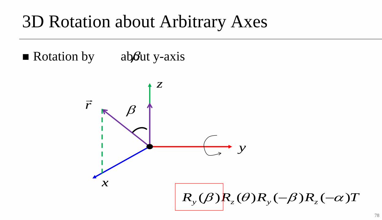
3D Rotation about Arbitrary Axes
◼ Rotation by about y-axis
x
y
z
r
x
TRRRRRT zyzyy )()()()()(1 −−−
78
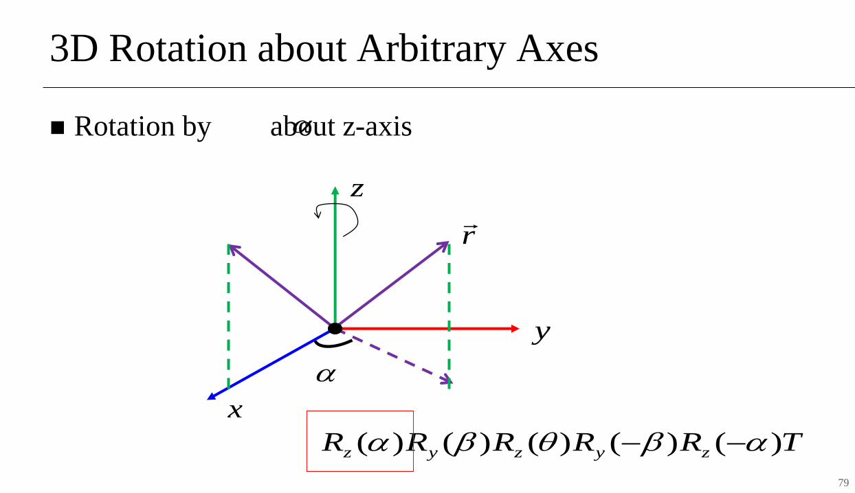
3D Rotation about Arbitrary Axes
◼ Rotation by about z-axis
x
y
z
r
TRRRRRT zyzyz )()()()()(1 −−−
79

3D Rotation about Arbitrary Axes
◼ Translate the object back to original point
x
y
z
r
TRRRRRT zyzyz )()()()()(1 −−−
80
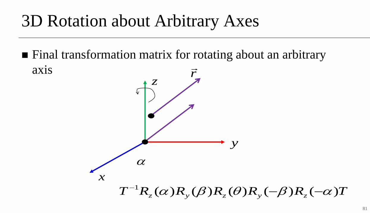
3D Rotation about Arbitrary Axes
◼ Final transformation matrix for rotating about an arbitrary
axis
x
y
z
r
TRRRRRT zyzyz )()()()()(1 −−−
81

3D Rotation about Arbitrary Axes
◼ Final transformation matrix for rotating about an arbitrary
axis
x
y
z
r
TRRRRRT zyzyz )()()()()(1 −−−
82

3D Rotation about Arbitrary Axes
◼ Final transformation matrix for rotating about an arbitrary
axis
TRRRRRT zyzyz )()()()()(1 −−−
=
1000
0
0
0
333231
232221
131211
rrr
rrr
rrr
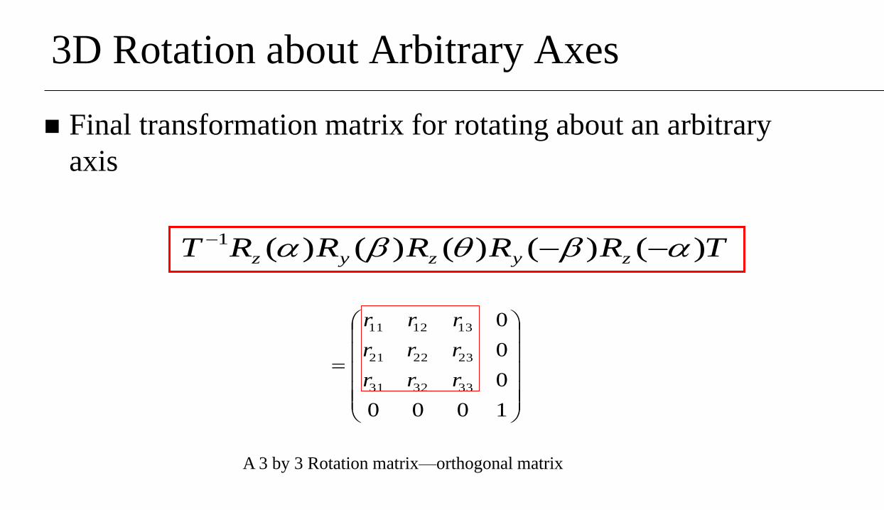
3D Rotation about Arbitrary Axes
◼ Final transformation matrix for rotating about an arbitrary
axis
TRRRRRT zyzyz )()()()()(1 −−−
A 3 by 3 Rotation matrix—orthogonal matrix
=
1000
0
0
0
333231
232221
131211
rrr
rrr
rrr

Rotation Matrices
◼ Orthonormal matrix:
◆orthogonal (columns/rows linearly independent)
◆normalized (columns/rows length of 1)
85
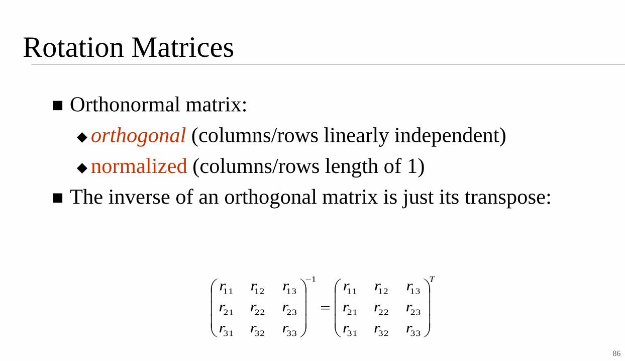
Rotation Matrices
◼ Orthonormal matrix:
◆orthogonal (columns/rows linearly independent)
◆normalized (columns/rows length of 1)
◼ The inverse of an orthogonal matrix is just its transpose:
86
T
rrr
rrr
rrr
rrr
rrr
rrr
=
−
333231
232221
131211
1
333231
232221
131211

Rotation Matrices
◼ Orthonormal matrix:
◆orthogonal (columns/rows linearly independent)
◆normalized (columns/rows length of 1)
◼ The inverse of an orthogonal matrix is just its transpose:
87
T
rrr
rrr
rrr
rrr
rrr
rrr
=
−
333231
232221
131211
1
333231
232221
131211
93IITK ME 761A Dr. J. Ramkumar
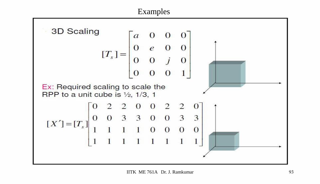
Examples
94IITK ME 761A Dr. J. Ramkumar
95IITK ME 761A Dr. J. Ramkumar
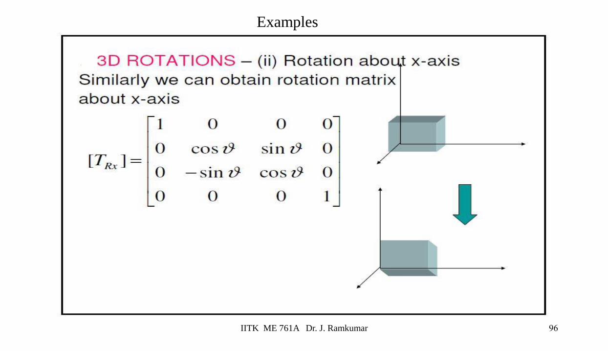
96IITK ME 761A Dr. J. Ramkumar
Examples
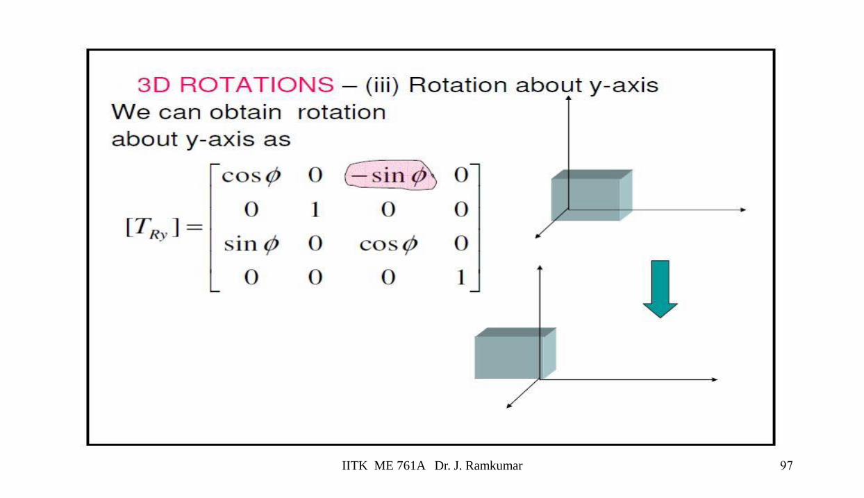
97IITK ME 761A Dr. J. Ramkumar

98IITK ME 761A Dr. J. Ramkumar
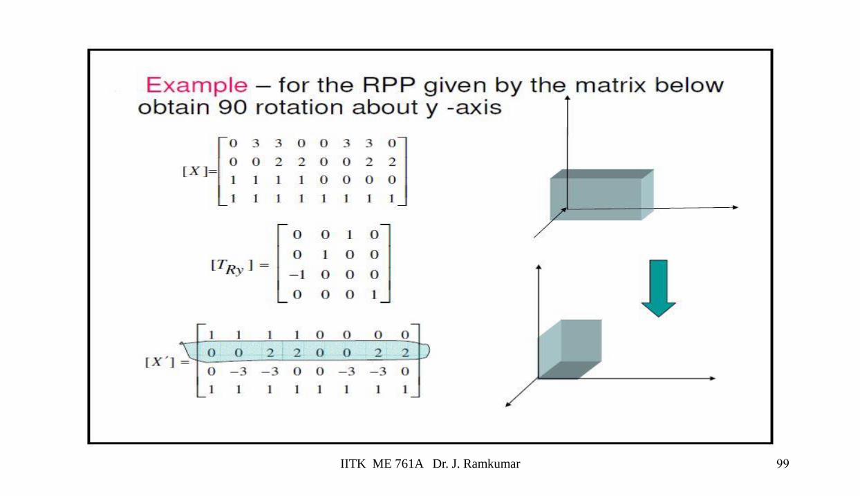
99IITK ME 761A Dr. J. Ramkumar

100IITK ME 761A Dr. J. Ramkumar
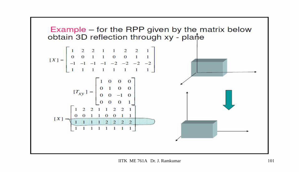
101IITK ME 761A Dr. J. Ramkumar
102IITK ME 761A Dr. J. Ramkumar
103IITK ME 761A Dr. J. Ramkumar
104IITK ME 761A Dr. J. Ramkumar
105IITK ME 761A Dr. J. Ramkumar
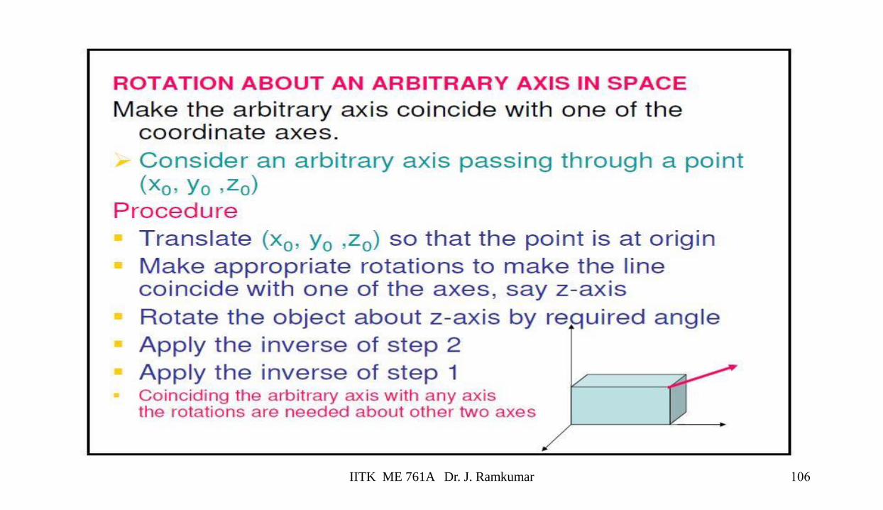
106IITK ME 761A Dr. J. Ramkumar
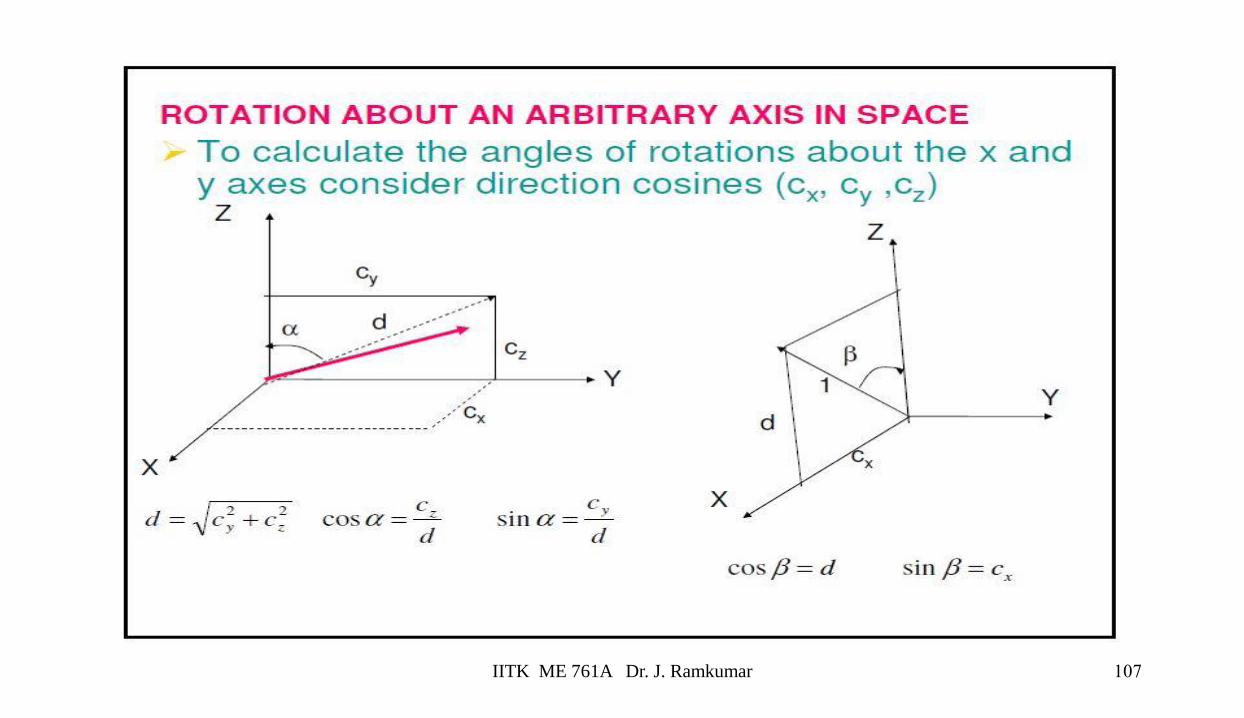
107IITK ME 761A Dr. J. Ramkumar
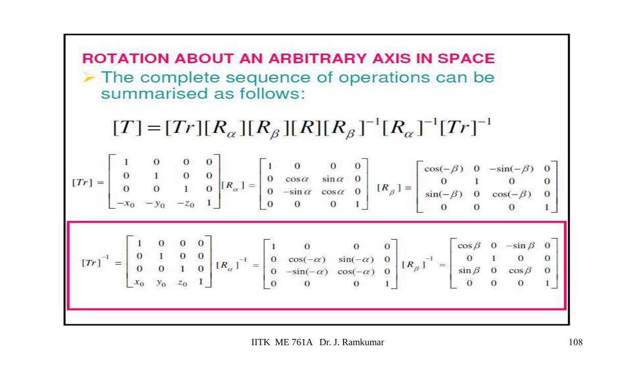
108IITK ME 761A Dr. J. Ramkumar
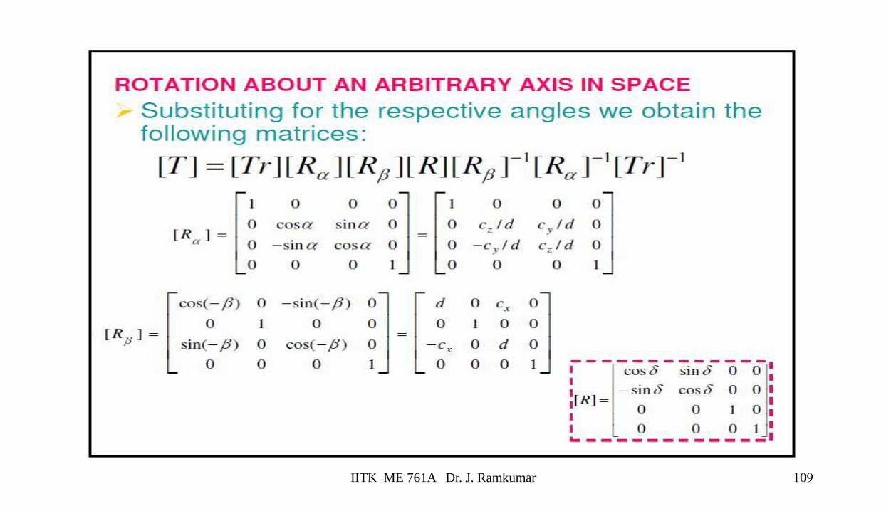
109IITK ME 761A Dr. J. Ramkumar
Splines and Bezier Curves
110IITK ME 761A Dr. J. Ramkumar
• |Representing Curves
– A number of small line-segments joined
• Interpolation
• Parametric equations
• Types of curve we study
– Natural Cubic Splines and Bezier Curves
• Derivation
• Implementation
111IITK ME 761A Dr. J. Ramkumar
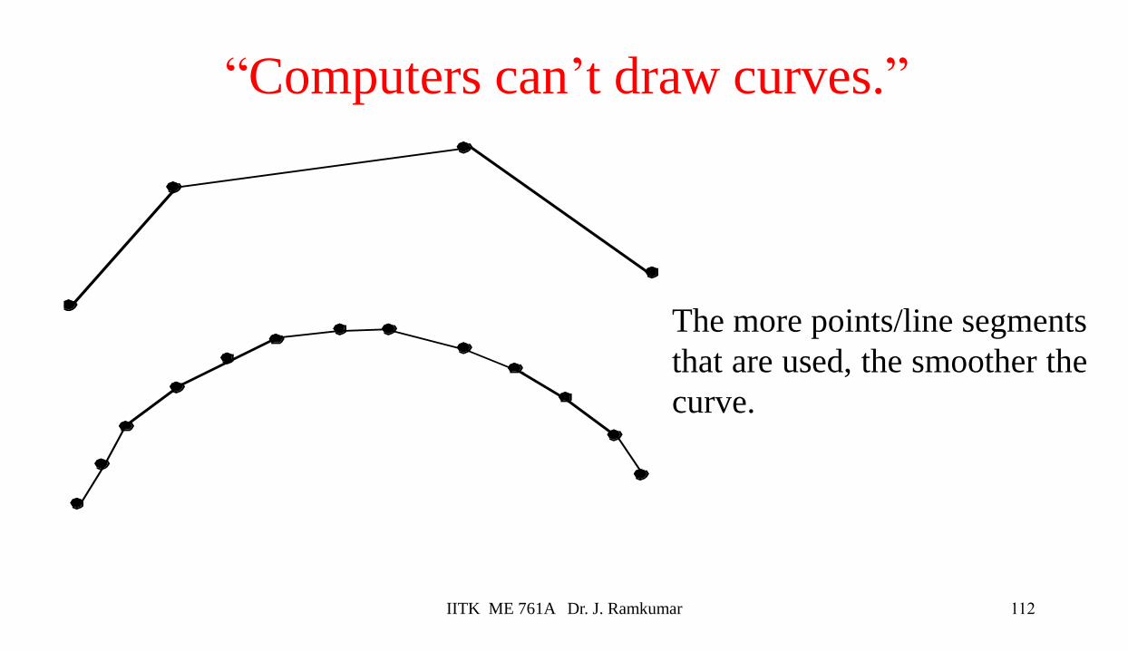
“Computers can’t draw curves.”
The more points/line segments
that are used, the smoother the
curve.
112IITK ME 761A Dr. J. Ramkumar
Why have curves ?
• Representation of “irregular surfaces”
• Example: Auto industry (car body design)
– Artist’s representation
– Clay / wood models
– Digitizing
– Surface modeling (“body in white”)
– Scaling and smoothening
– Tool and die Manufacturing
113IITK ME 761A Dr. J. Ramkumar

Curve representation
• Problem: How to represent a curve easily and efficiently
• “Brute force and ignorance” approaches:
• storing a curve as many small straight line segments– doesn’t work well when scaled
– inconvenient to have to specify so many points
– need lots of points to make the curve look smooth
• working out the equation that represents the curve– difficult for complex curves
– moving an individual point requires re-calculation of the entire curve
114IITK ME 761A Dr. J. Ramkumar
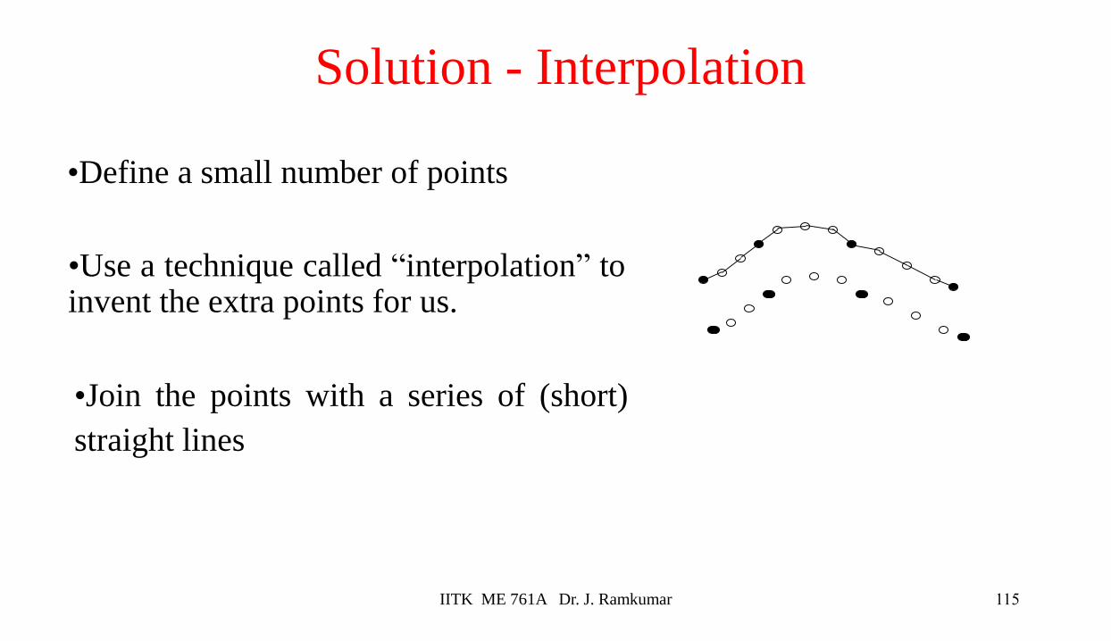
Solution - Interpolation
•Define a small number of points
•Use a technique called “interpolation” toinvent the extra points for us.
•Join the points with a series of (short)
straight lines
115IITK ME 761A Dr. J. Ramkumar
The need for smoothness
• So far, mostly polygons
• Can approximate any geometry, but
– Only approximate
– Need lots of polygons to hide discontinuities
• Storage problems
– Math problems
• Normal direction
• Texture coordinates
– Not very convenient as modeling tool
• Gets even worse in animation
– Almost always need smooth motion
116IITK ME 761A Dr. J. Ramkumar
Geometric modeling
• Representing world geometry in the computer
– Discrete vs. continuous again
• At least some part has to be done by a human
– Will see some automatic methods soon
• Reality: humans are discrete in their actions
• Specify a few points, have computer create something which
“makes sense”
– Examples: goes through points, goes “near” points
117IITK ME 761A Dr. J. Ramkumar
Requirements
• Want mathematical smoothness
– Some number of continuous derivatives of P
• Local control
– Local data changes have local effect
• Continuous with respect to the data
– No wiggling if data changes slightly
• Low computational effort
118IITK ME 761A Dr. J. Ramkumar

A solution
• Use SEVERAL polynomials
• Complete curve consists of several pieces
• All pieces are of low order
– Third order is the most common
• Pieces join smoothly
• This is the idea of spline curves
– or just “splines”
119IITK ME 761A Dr. J. Ramkumar
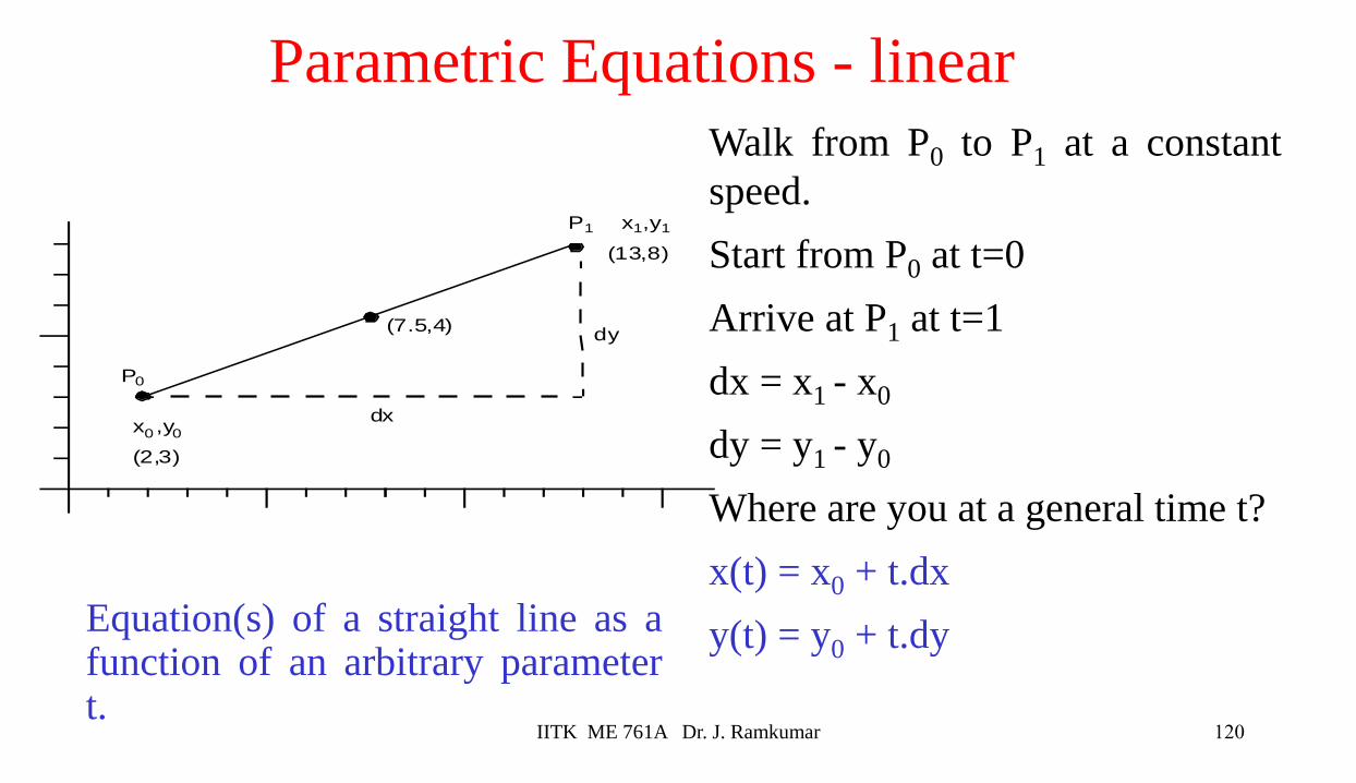
Parametric Equations - linear
x0 ,y0
x1,y1
dy
dx
(13,8)
(2,3)
P0
P1
(7.5,4)
Walk from P0 to P1 at a constant
speed.
Start from P0 at t=0
Arrive at P1 at t=1
dx = x1 - x0
dy = y1 - y0
Where are you at a general time t?
x(t) = x0 + t.dx
y(t) = y0 + t.dyEquation(s) of a straight line as afunction of an arbitrary parametert.
120IITK ME 761A Dr. J. Ramkumar
Why use parametric equations?
• One, two, three or n-dimensional representation is
possible
• Can handle “infinite slope” of tangents
• Can represent multi-valued functions
122IITK ME 761A Dr. J. Ramkumar

• Natural Cubic Spline
• Bezier Curves
123IITK ME 761A Dr. J. Ramkumar
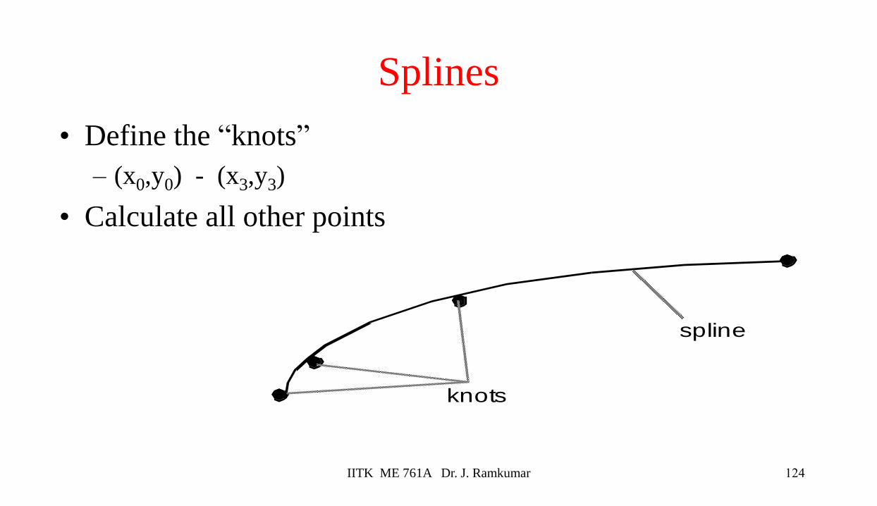
Splines
• Define the “knots”
– (x0,y0) - (x3,y3)
• Calculate all other points
spline
knots
124IITK ME 761A Dr. J. Ramkumar

Continuity
• Parametric continuity Cx
– Only P is continuous: C0
• Positional continuity
– P and first derivative dP/du are continuous: C1
• Tangential continuity
– P + first + second: C2
• Curvature continuity
• Geometric continuity Gx
– Only directions have to match
125IITK ME 761A Dr. J. Ramkumar
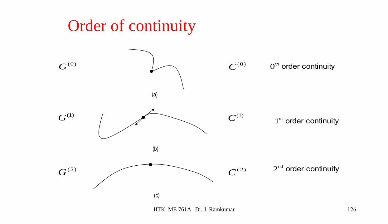
)0(G
)1(G
(a)
(b)
(c)
continuity order th0
continuity order st1
continuity order nd2)2(G
)0(C
)1(C
)2(C
Order of continuity
126IITK ME 761A Dr. J. Ramkumar
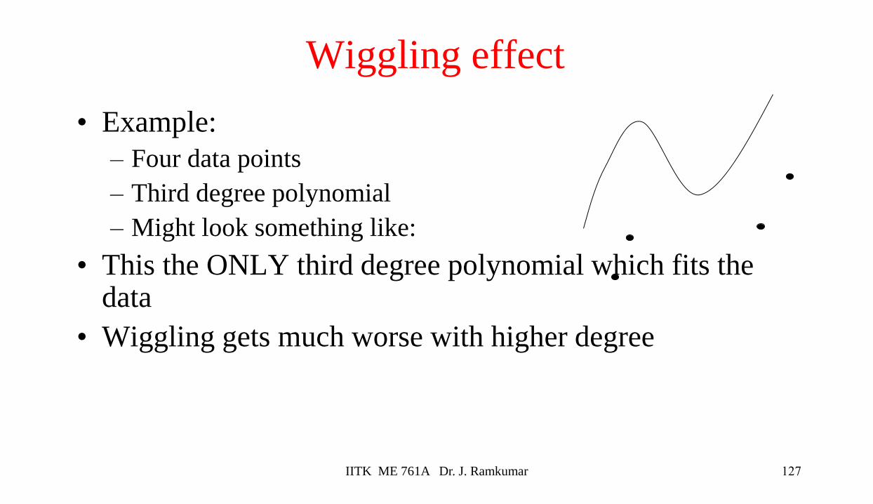
Wiggling effect
• Example:
– Four data points
– Third degree polynomial
– Might look something like:
• This the ONLY third degree polynomial which fits the data
• Wiggling gets much worse with higher degree
127IITK ME 761A Dr. J. Ramkumar
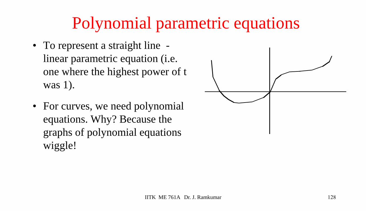
Polynomial parametric equations
• To represent a straight line -
linear parametric equation (i.e.
one where the highest power of t
was 1).
• For curves, we need polynomial
equations. Why? Because the
graphs of polynomial equations
wiggle!
128IITK ME 761A Dr. J. Ramkumar

Natural Cubic Spline
• spline, n. 1 A long narrow and relatively thin piece or strip of wood, metal, etc. 2 A flexible strip of wood or rubber used by draftsmen in laying out broad sweeping curves, as in railroad work.
• A natural spline defines the curve that minimizes the potential energy of an idealized elastic strip.
129IITK ME 761A Dr. J. Ramkumar
• A natural cubic spline defines a curve, in which the points P(u) that define each segment of the spline are represented as a cubic P(u) = a0 + a1u + a2u
2 + a3u3
• Where u is between 0 and 1 and a0, a1, a2 and a3 are (as
yet) undetermined parameters.
• We assume that the positions of n+1 control points Pk,
where k = 0, 1,…, n are given, and the 1st and 2nd
derivatives of P(u) are continuous at each interior control
point.
130IITK ME 761A Dr. J. Ramkumar
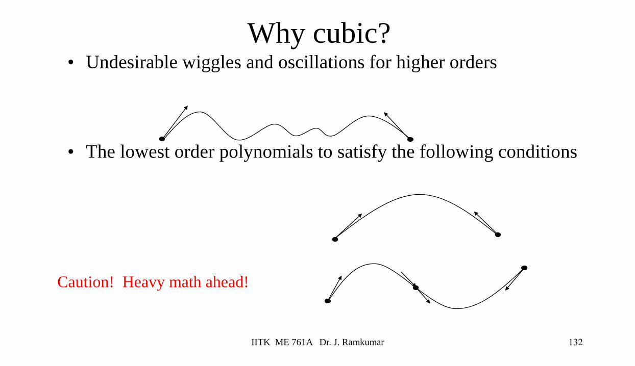
• Undesirable wiggles and oscillations for higher orders
• The lowest order polynomials to satisfy the following conditions
Why cubic?
Caution! Heavy math ahead!
132IITK ME 761A Dr. J. Ramkumar
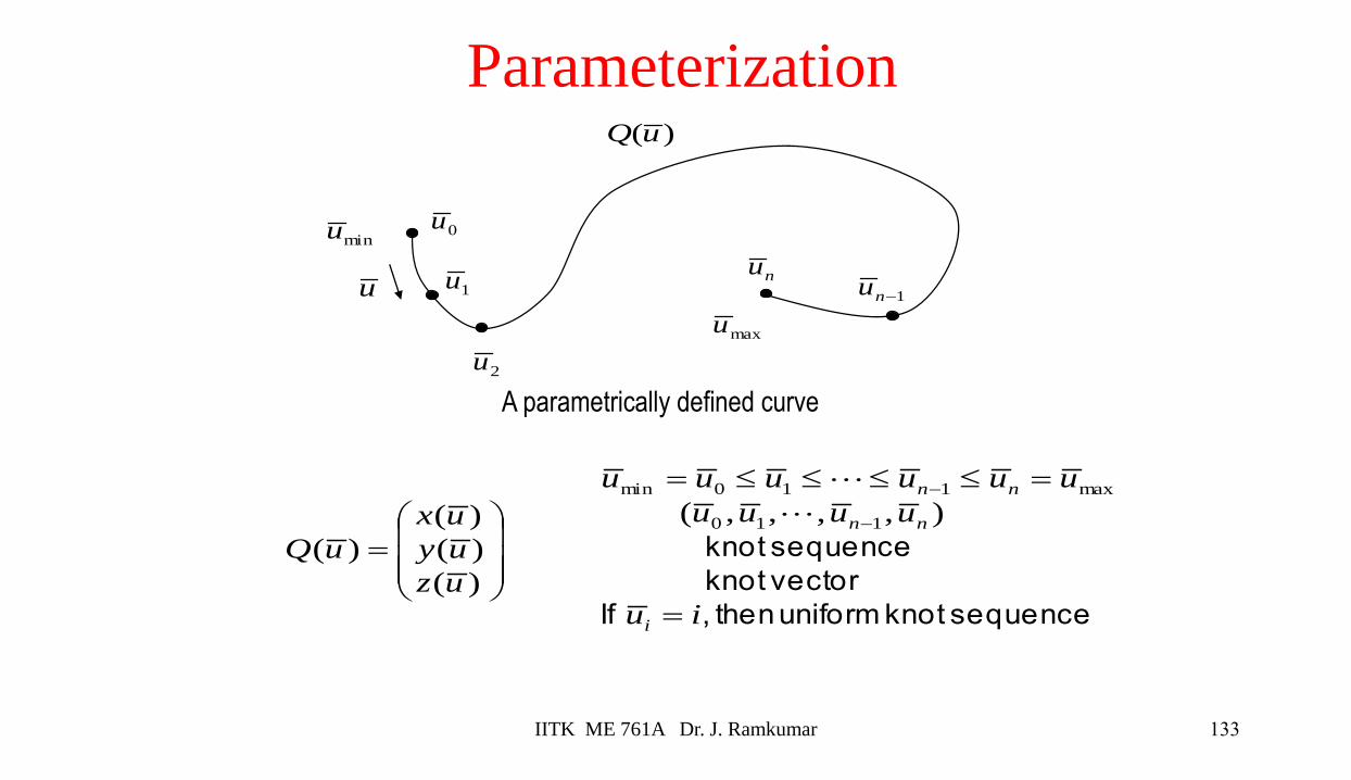
minu
maxu
u
0u
1u
2u
nu1−nu
)(uQ
A parametrically defined curve
=
)(
)(
)(
)(
uz
uy
ux
uQ
sequenceknot uniform then , If
vectorknot
sequenceknot
iu
uuuu
uuuuuu
i
nn
nn
=
==
−
−
),,,,( 110
max110min
Parameterization
133IITK ME 761A Dr. J. Ramkumar
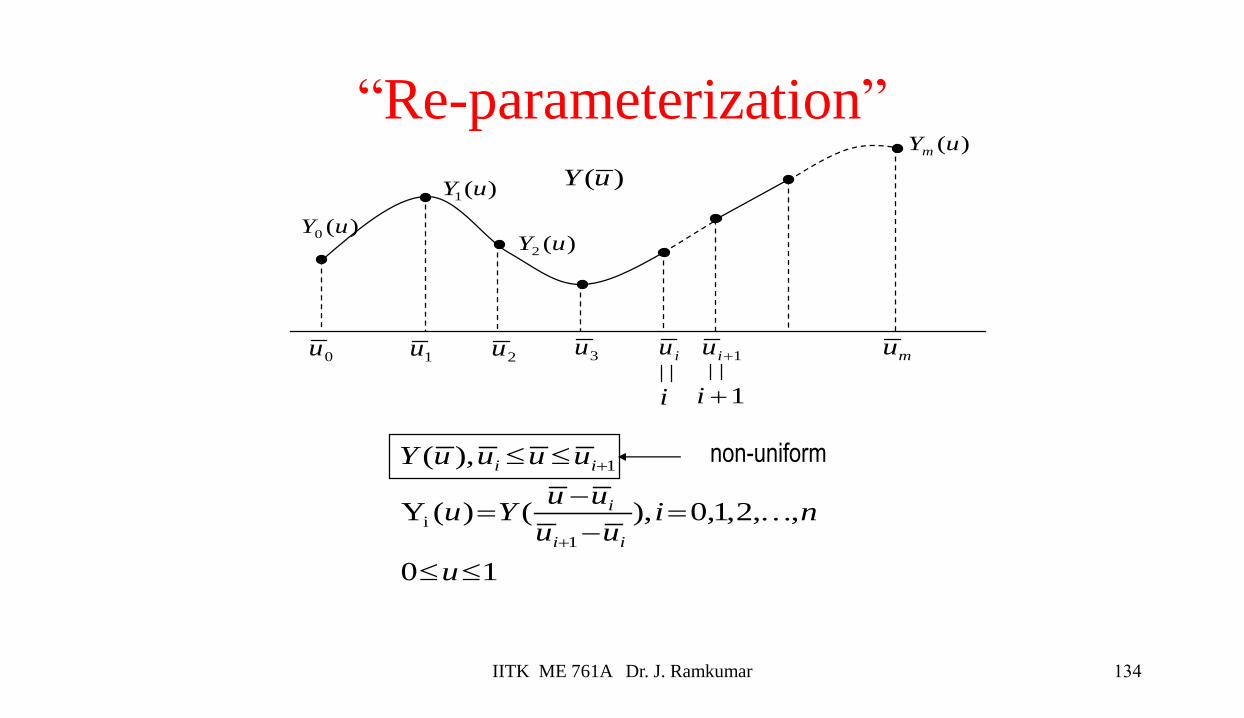
0u 1u 2u 3u iu 1+iu mu
)(uY)(1 uY
)(0 uY)(2 uY
)(uYm
i 1+i
10
,,2,1,0),()(Y
),(
1
i
1
=−
−=
+
+
u
niuu
uuYu
uuuuY
ii
i
ii
non-uniform
“Re-parameterization”
134IITK ME 761A Dr. J. Ramkumar
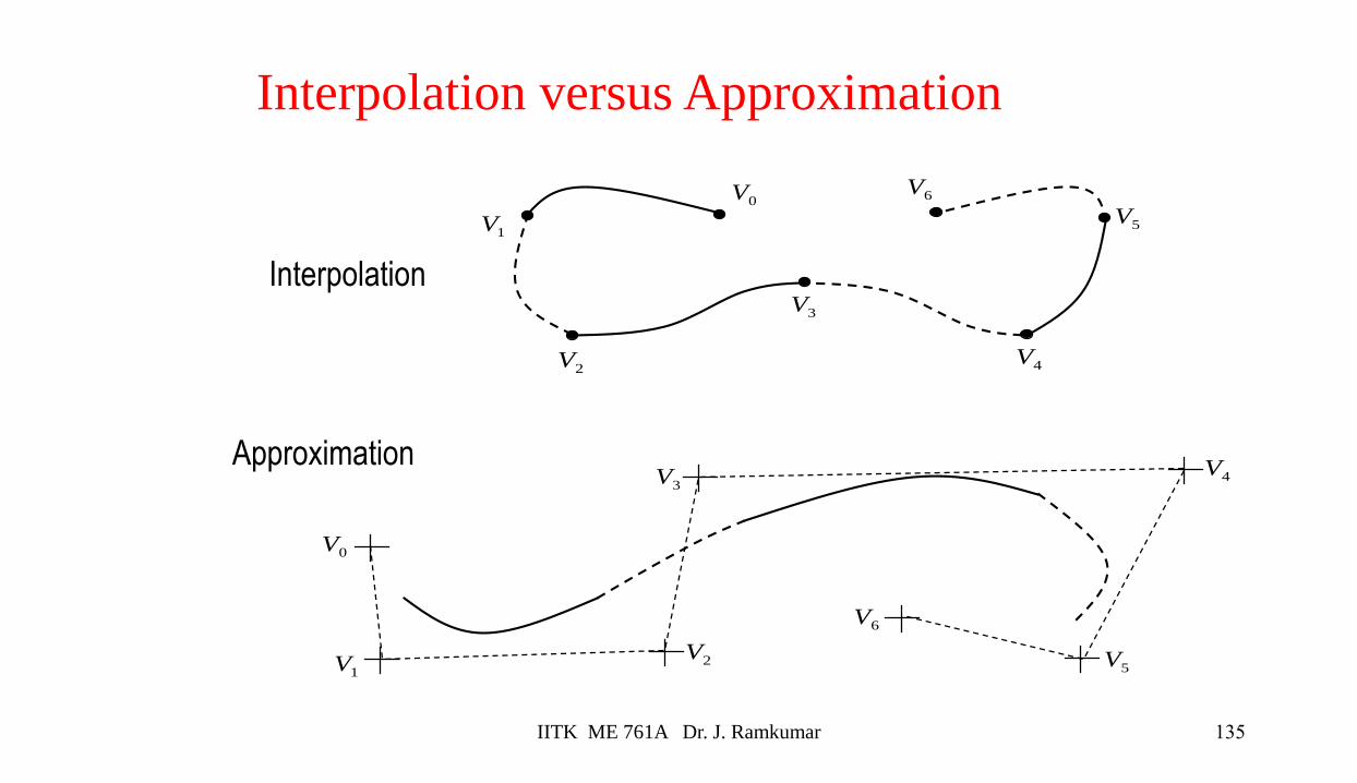
0V
1V
2V
3V
4V
5V6V
Interpolation
0V
1V 2V
3V 4V
5V
6V
Approximation
Interpolation versus Approximation
135IITK ME 761A Dr. J. Ramkumar
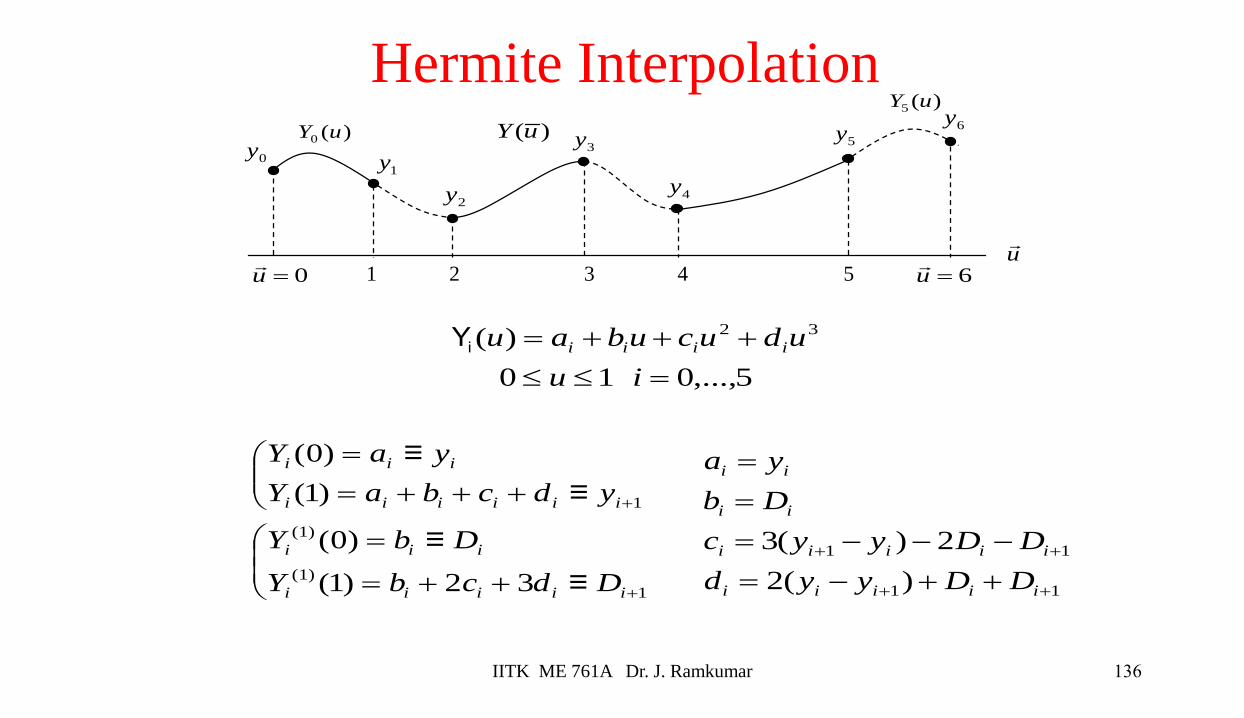
0y1y
2y
3y
4y
5y6y
)(0 uY )(uY
)(5 uY
u
6=u
0=u
++=
=
+++=
=
+
+
1
)1(
)1(
1
≡32)1(
≡)0(
≡)1(
≡)0(
iiiii
iii
iiiiii
iii
DdcbY
DbY
ydcbaY
yaY
5,...,010
)( 32
=
+++=
iu
uducubau iiii
Yi
11
11
)(2
2)(3
++
++
++−=
−−−=
=
=
iiiii
iiiii
ii
ii
DDyyd
DDyyc
Db
ya
1 2 3 4 5
Hermite Interpolation
136IITK ME 761A Dr. J. Ramkumar
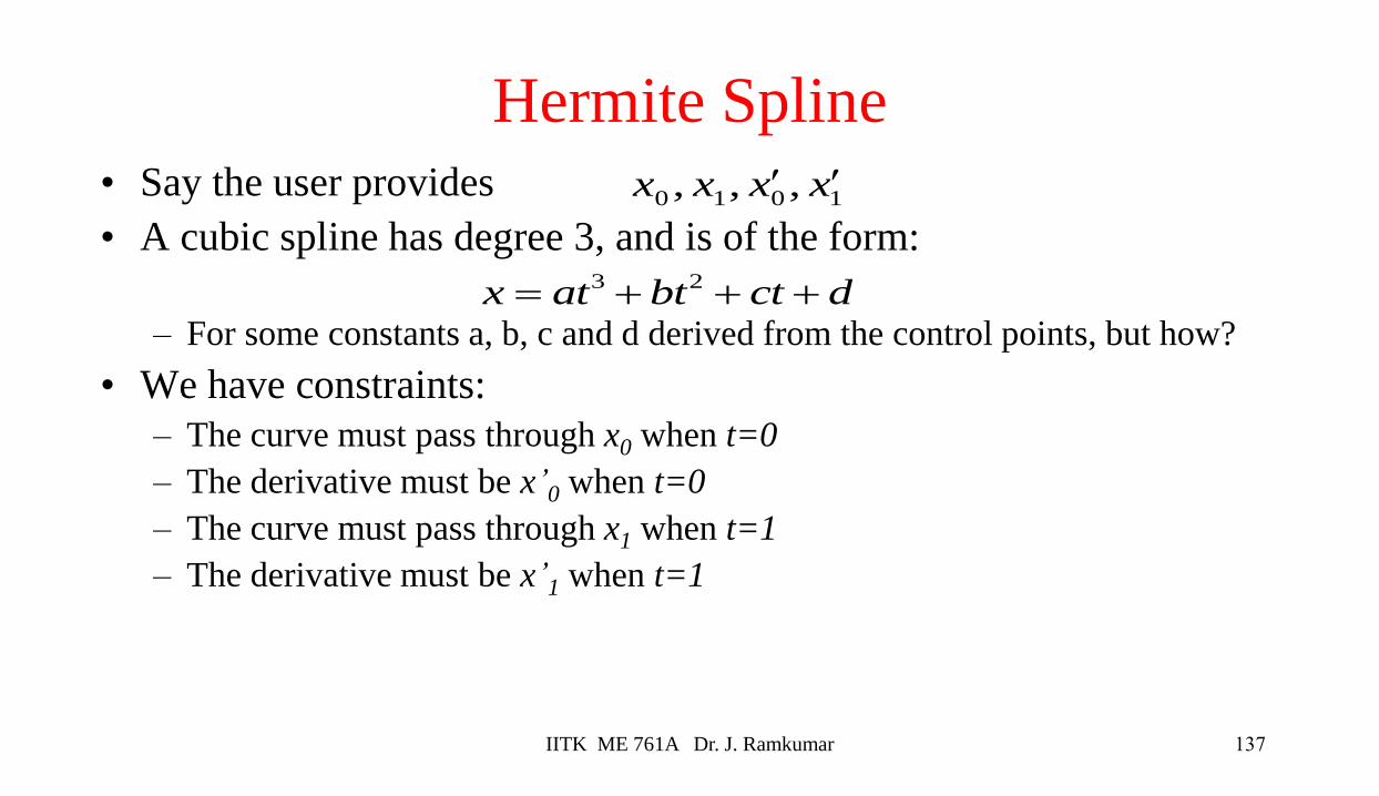
Hermite Spline• Say the user provides
• A cubic spline has degree 3, and is of the form:
– For some constants a, b, c and d derived from the control points, but how?
• We have constraints:
– The curve must pass through x0 when t=0
– The derivative must be x’0 when t=0
– The curve must pass through x1 when t=1
– The derivative must be x’1 when t=1
dctbtatx +++= 23
1010 ,,, xxxx
137IITK ME 761A Dr. J. Ramkumar
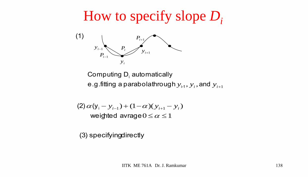
10
))(1() 11
−−+− +−
avrage hted weig
(y (2) i iii yyy
directly specifying (3)
1,, +ii yyy and through parabola a fitting e.g.
llyautomatica D Computing
(1)
-1i
i
1−iy
iy
1+iy1−iP
iP
1+iP
How to specify slope Di
138IITK ME 761A Dr. J. Ramkumar

Hermite Spline
A Hermite spline is a curve for which the user provides:
– The endpoints of the curve
– The parametric derivatives of the curve at the endpoints
• The parametric derivatives are dx/dt, dy/dt, dz/dt
– That is enough to define a cubic Hermite spline, more derivatives are required for higher order curves
139IITK ME 761A Dr. J. Ramkumar
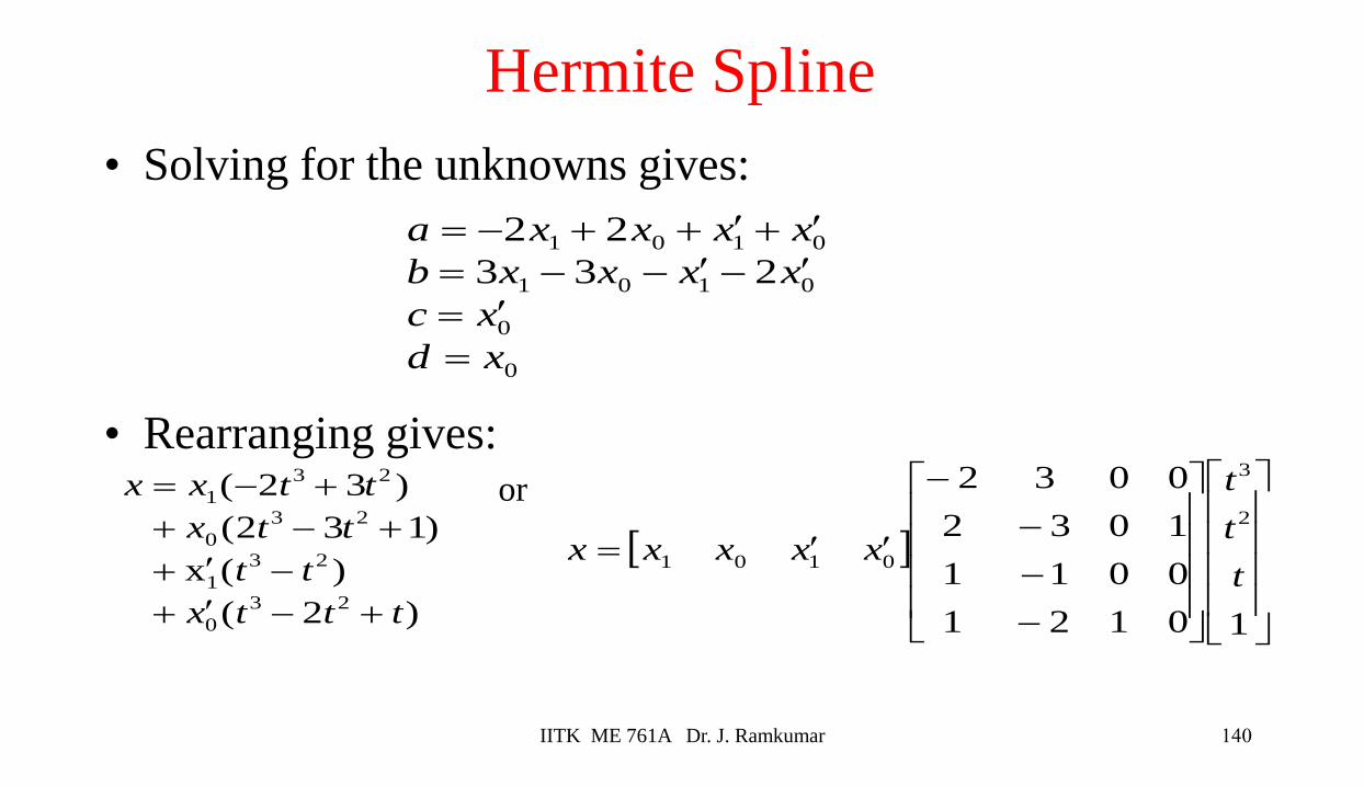
Hermite Spline
• Solving for the unknowns gives:
• Rearranging gives:
0
0
0101
0101
233
22
xd
xc
xxxxb
xxxxa
=
=
−−−=
+++−=
)2(
)(x
)132(
)32(
23
0
23
1
23
0
23
1
tttx
tt
ttx
ttxx
+−+
−+
+−+
+−=
−
−
−
−
=
10121
0011
1032
00322
3
0101t
t
t
xxxxx
or
140IITK ME 761A Dr. J. Ramkumar
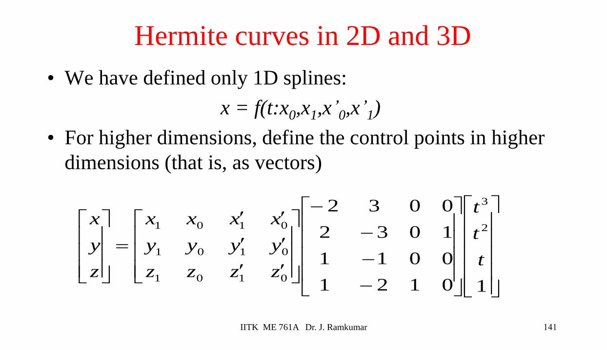
Hermite curves in 2D and 3D
• We have defined only 1D splines:
x = f(t:x0,x1,x’0,x’1)
• For higher dimensions, define the control points in higher
dimensions (that is, as vectors)
−
−
−
−
=
10121
0011
1032
00322
3
0101
0101
0101
t
t
t
zzzz
yyyy
xxxx
z
y
x
141IITK ME 761A Dr. J. Ramkumar
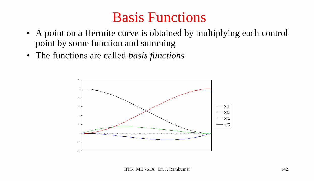
Basis Functions• A point on a Hermite curve is obtained by multiplying each control
point by some function and summing
• The functions are called basis functions
-0.4
-0.2
0
0.2
0.4
0.6
0.8
1
1.2
x1
x0
x'1
x'0
142IITK ME 761A Dr. J. Ramkumar
0V
1V
2V
3V
4V
5V6V
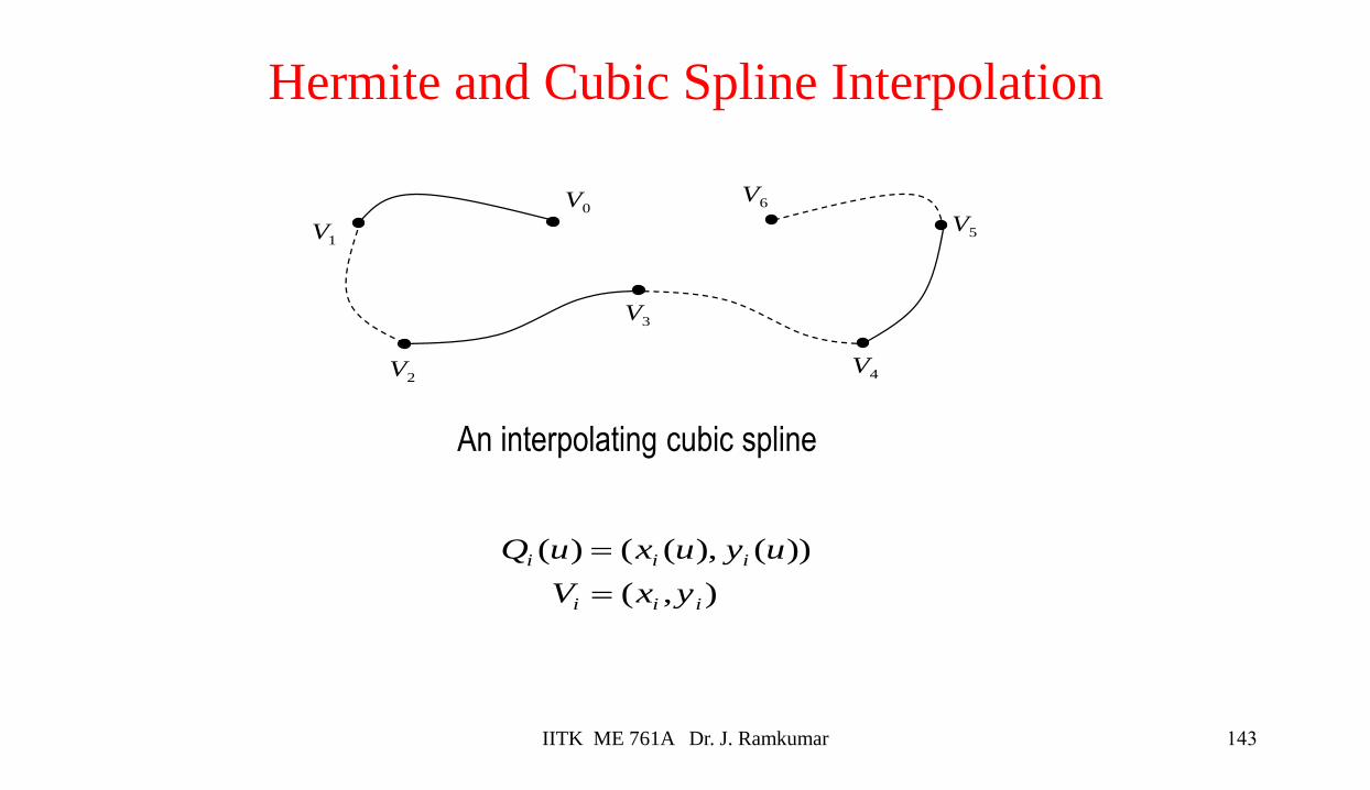
An interpolating cubic spline
),(
))(),(()(
iii
iii
yxV
uyuxuQ
=
=
Hermite and Cubic Spline Interpolation
143IITK ME 761A Dr. J. Ramkumar
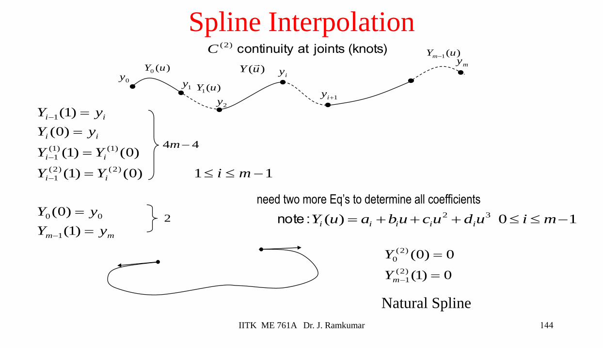
(knots) jointsat continuity )2(C
0y1y
2y
iy
1+iy
my)(0 uY )(uY
)(1 uYm−
)(1 uY
mm
ii
ii
ii
ii
yY
yY
miYY
YY
yY
yY
=
=
−=
=
=
=
−
−
−
−
)1(
)0(
11 )0()1(
)0()1(
)0(
)1(
1
00
)2()2(
1
)1()1(
1
1
44 −m
2
need two more Eq’s to determine all coefficients
10)( 32 −+++= miuducubauY iiiii : note
Spline Interpolation
0)1(
0)0(
)2(
1
)2(
0
=
=
−mY
Y
Natural Spline
144IITK ME 761A Dr. J. Ramkumar
11
)(34
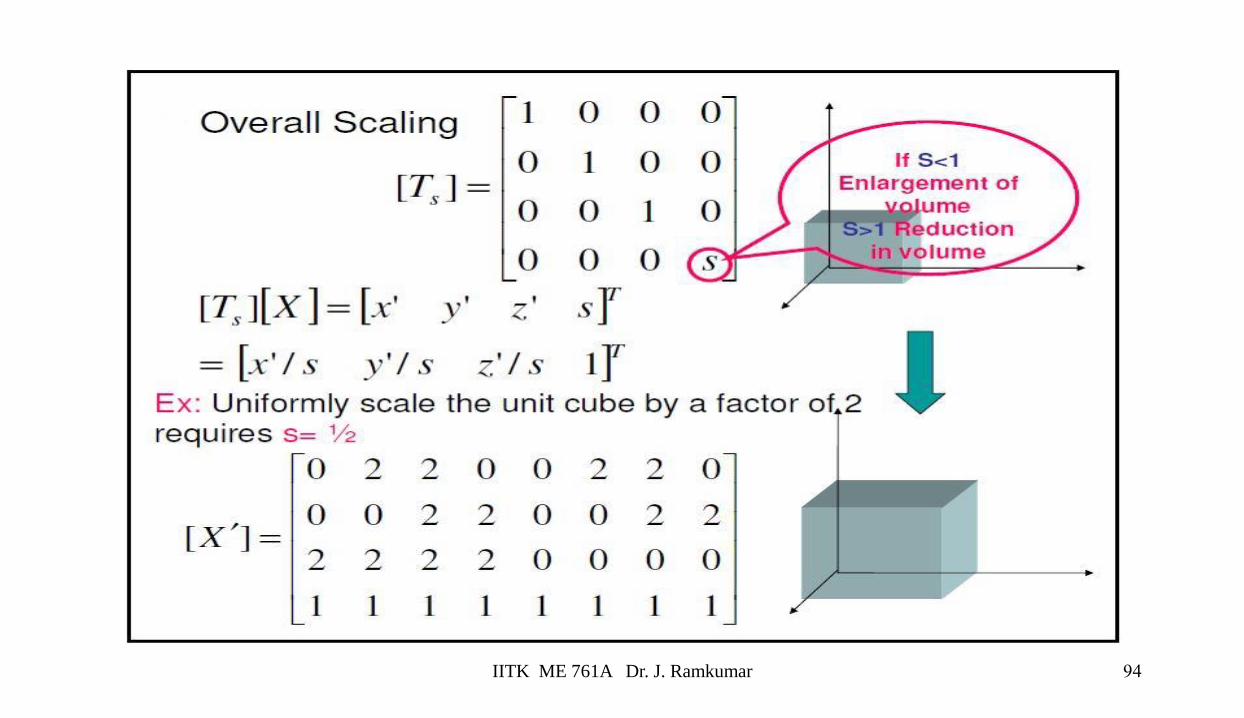
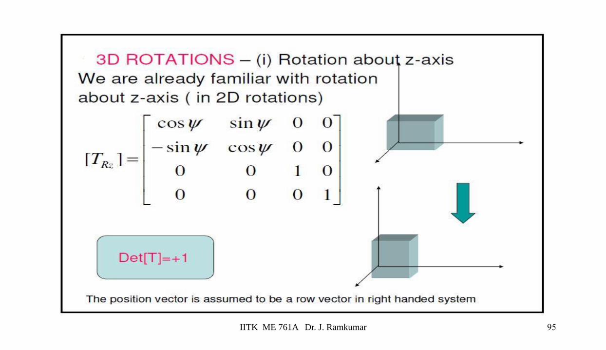
)(2
2)(3
262
1111
11
11
11
−
−=++
++−=
−−−=
=
=
=+
−++−
++
++
−−
mi
yyDDD
DDyyd
DDyyc
Db
ya
cdc
iiiii
iiiii
iiiii
ii
ii
iii
tion,simplifica and onsubstitutiBy
(4)
0)1(
0)0(
)1(
)0(
)0()1(
)0()1(
)0(
)1(
)2(
1
)2(
0
1
00
)2()2(
1
)1()1(
1
1
=
=
=
=
=
=
=
=
−
−
−
−
−
m
mm
ii
ii
ii
ii
Y
Y
yY
yY
YY
YY
yY
yY
(8)
(7)
(6)
(5)
(4)
(3)
(2)
(1)
11 − mi
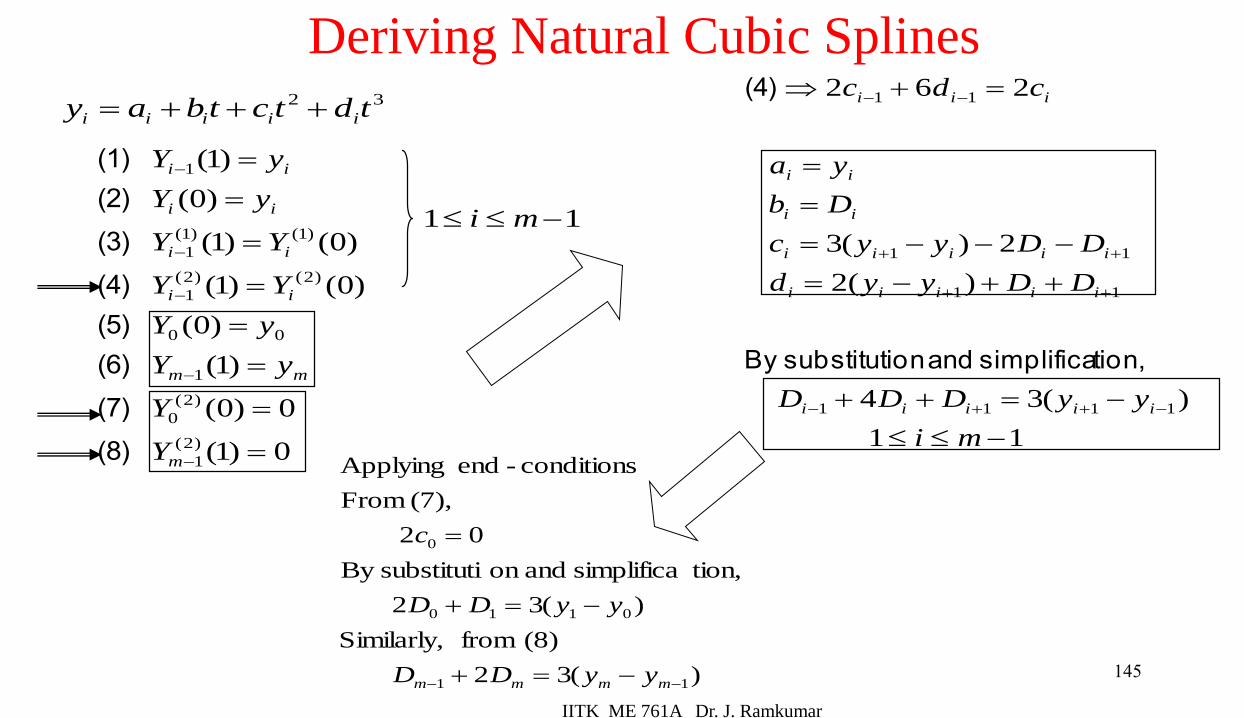
32 tdtctbay iiiii +++=
Deriving Natural Cubic Splines
)(32
(8) from Similarly,
)(32
tion,simplifica and onsubstitutiBy
02
(7), From
conditions-end Applying
11
0110
0
−− −=+
−=+
=
mmmm yyDD
yyDD
c
145
IITK ME 761A Dr. J. Ramkumar
−
−
−
−
=
−
−
)(3
)(3
)(3
)(3
21
141
....
141
141
141
12
1
2
02
01
1
0
mm
mm
m yy
yy
yy
yy
D
D
D
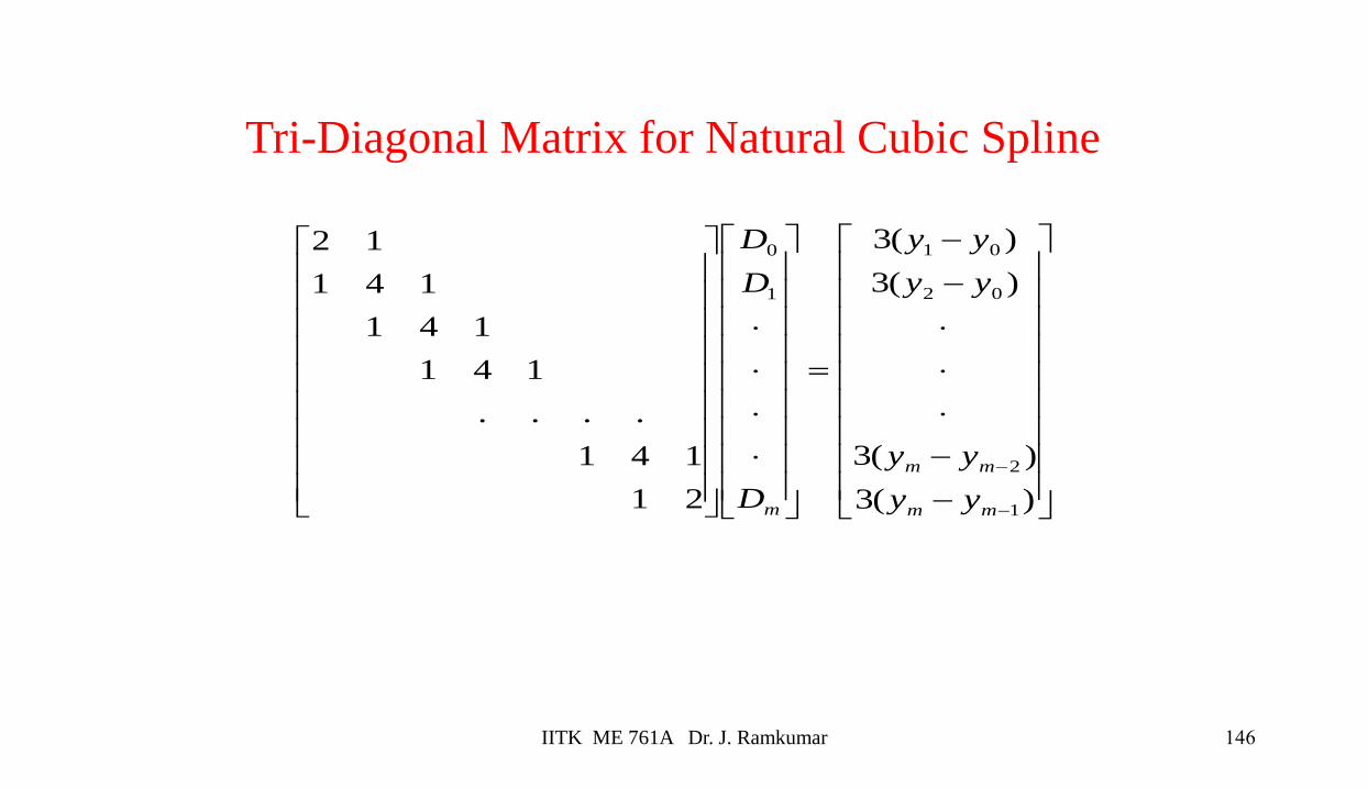
Tri-Diagonal Matrix for Natural Cubic Spline
146IITK ME 761A Dr. J. Ramkumar
iP
mP0P
2P
1P
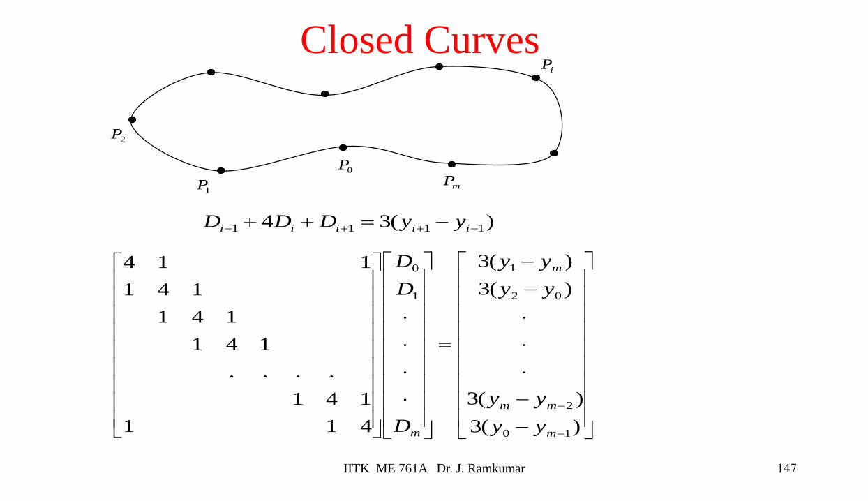
)(34 1111 −++− −=++ iiiii yyDDD
−
−
−
−
=
−
−
)(3
)(3
)(3
)(3
411
141
....
141
141
141
114
10
2
02
1
1
0
m
mm
m
m yy
yy
yy
yy
D
D
D
Closed Curves
147IITK ME 761A Dr. J. Ramkumar
IITK ME 761A Dr. J. Ramkumar 148
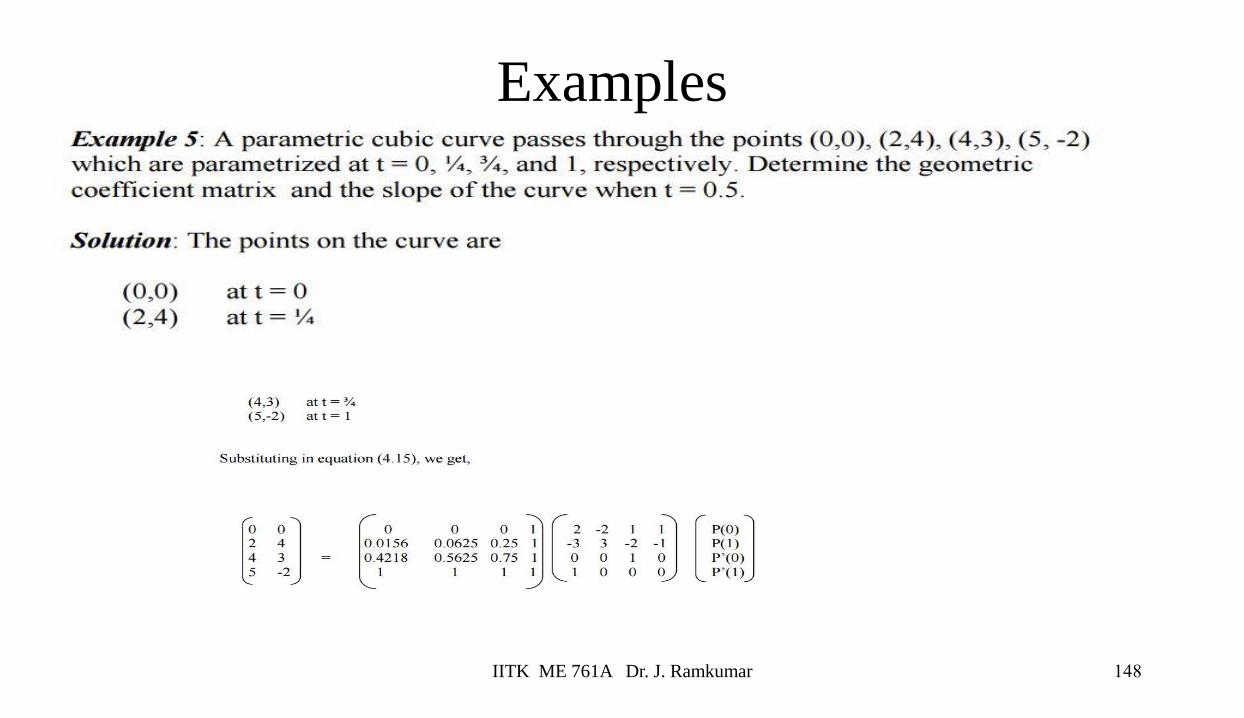
Examples

IITK ME 761A Dr. J. Ramkumar
149

IITK ME 761A Dr. J. Ramkumar 150
Exercise
Bezier Curves
• An alternative to splines
• M. Bezier was a French mathematician who worked for the Renault
motor car company.
• He invented his curves to allow his firm’s computers to describe the
shape of car bodies.
151IITK ME 761A Dr. J. Ramkumar
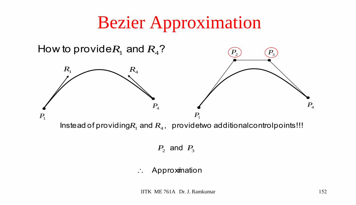
? and provide to How 41 R R
1P
4P
1R4R
mation Approxi
and
!!! points control additional two provide , and providing of Instead
32
41
PP
RR
1P
4P
2P3P
Bezier Approximation
152IITK ME 761A Dr. J. Ramkumar
Bezier curves
• Typically, cubic polynomials
• Similar to Hermite interpolation
– Special way of specifying end tangents
• Requires special set of coefficients
• Need four points
– Two at the ends of a segment
– Two control tangent vectors
153IITK ME 761A Dr. J. Ramkumar
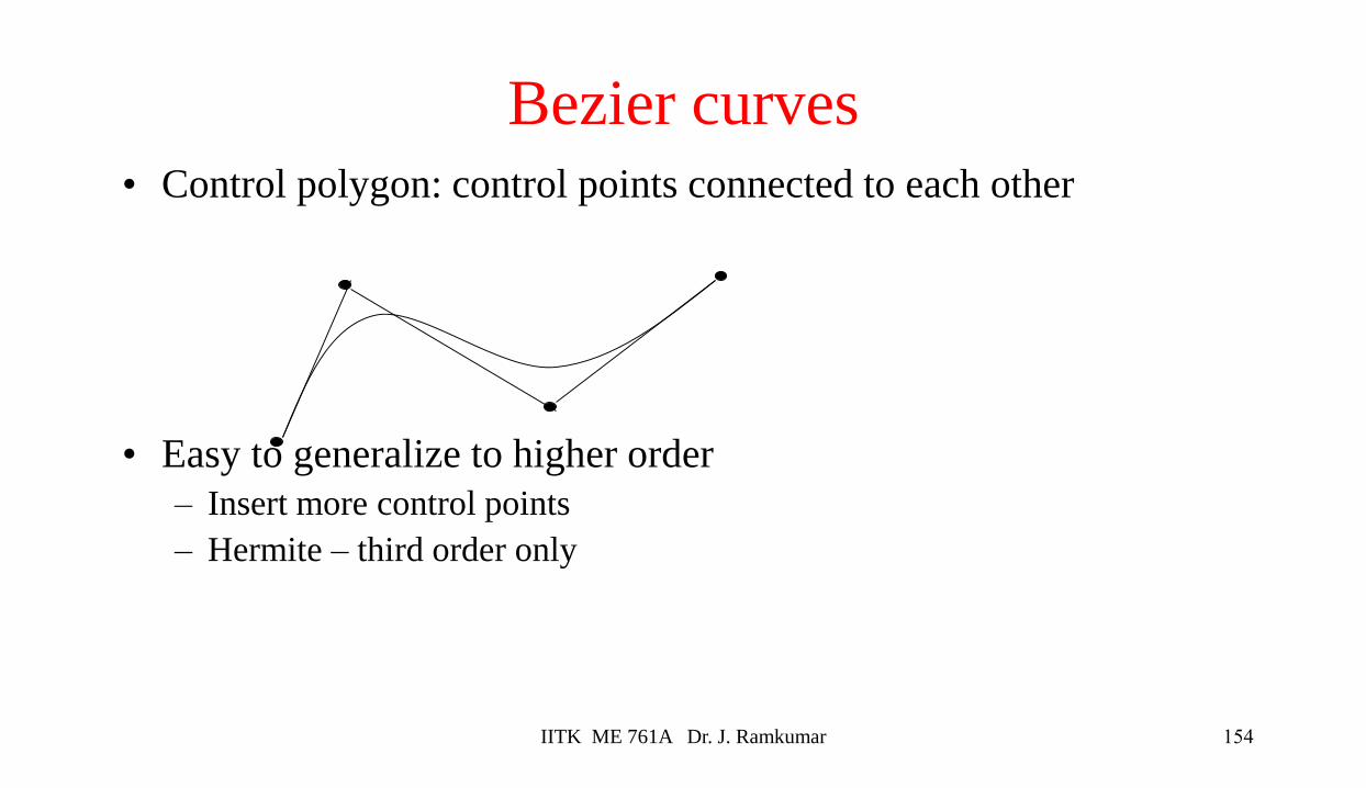
Bezier curves
• Control polygon: control points connected to each other
• Easy to generalize to higher order
– Insert more control points
– Hermite – third order only
154IITK ME 761A Dr. J. Ramkumar
De Casteljau algorithm
• Can compute any point on the curve in a few iterations
• No polynomials, pure geometry
• Repeated linear interpolation
– Repeated order of the curve times
• The algorithm can be used as definition of the curve
155IITK ME 761A Dr. J. Ramkumar
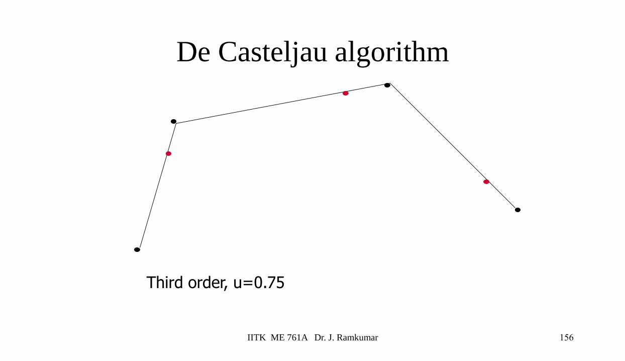
De Casteljau algorithm
Third order, u=0.75
156IITK ME 761A Dr. J. Ramkumar
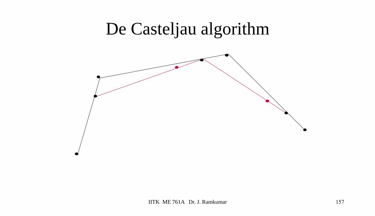
De Casteljau algorithm
157IITK ME 761A Dr. J. Ramkumar
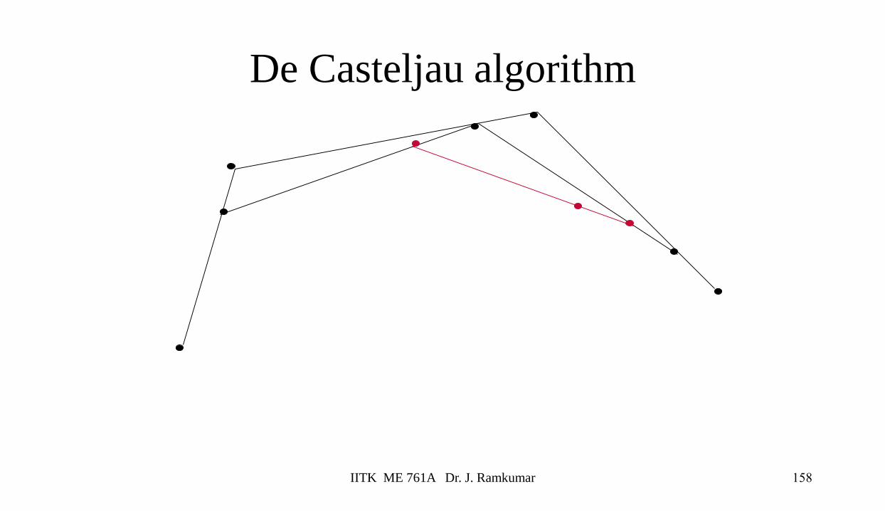
De Casteljau algorithm
158IITK ME 761A Dr. J. Ramkumar
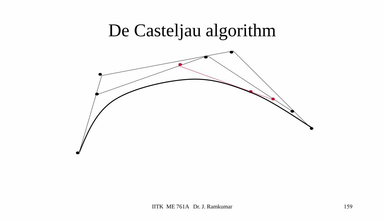
De Casteljau algorithm
159IITK ME 761A Dr. J. Ramkumar
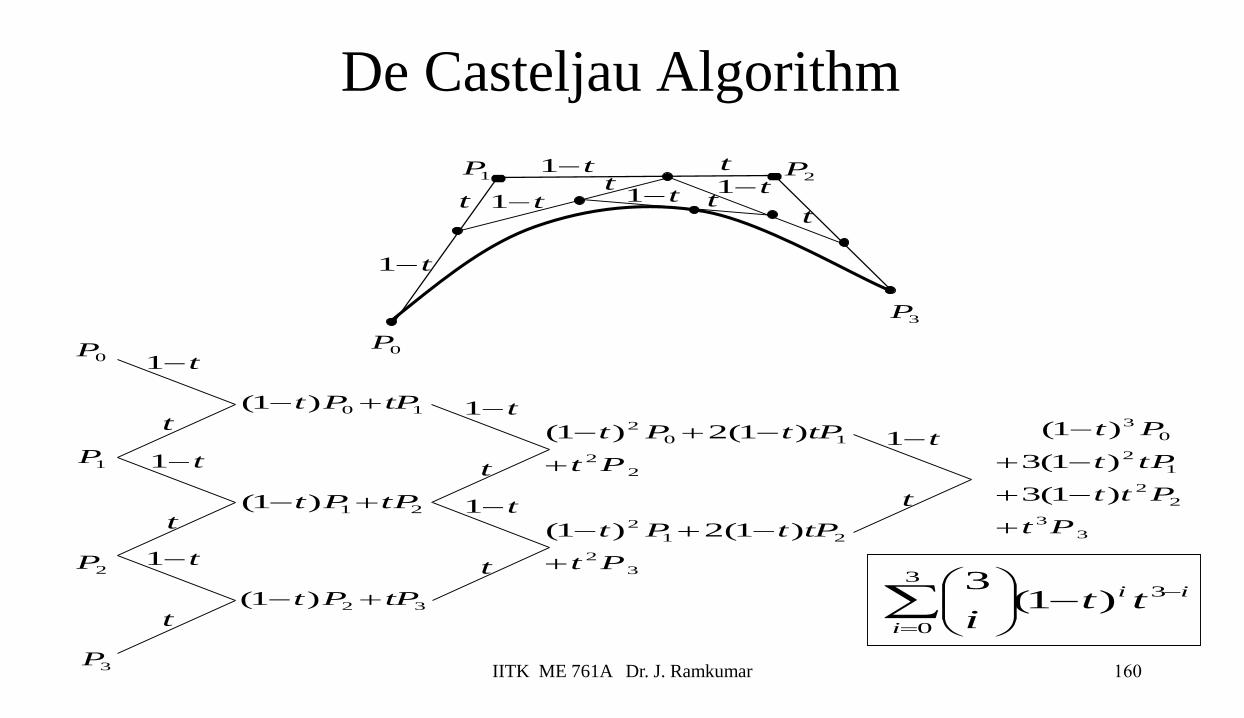
De Casteljau Algorithm
3P
1P2P
t
t−1
t−1 t−1
t−1t−1
t
tt
t
0P0P
1P
2P
3P
t−1
t
t−1
t
t−1
t
10)1( tPPt +−
21)1( tPPt +−
32)1( tPPt +−
t−1
t
t−1
t
2
2
10
2 )1(2)1(
Pt
tPtPt
+
−+−
3
2
21
2 )1(2)1(
Pt
tPtPt
+
−+−
t−1
t
3
3
2
2
1
2
0
3
)1(3
)1(3
)1(
Pt
Ptt
tPt
Pt
+
−+
−+
−
ii
i
tti
−
=
−
3
3
0
)1(3
160IITK ME 761A Dr. J. Ramkumar
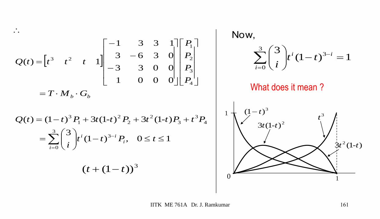
0
1
1
3)1( t−
2)1(3 -tt
3t
)1(3 2 -tt
Now,
1)1(3
33
0
=−
−
=
ii
i
tti
What does it mean ?
10)1(3
)1(3)1(3)1()(
0001
0033
0363
1331
1)(
33
0
4
3
3
2
2
2
1
3
4
3
2
1
23
−
=
+++−=
=
−
−
−
=
−
=
t, Ptti
PtP-ttP-ttPttQ
GMT
P
P
P
P
ttttQ
i
ii
i
bb
3))1(( tt −+
161IITK ME 761A Dr. J. Ramkumar
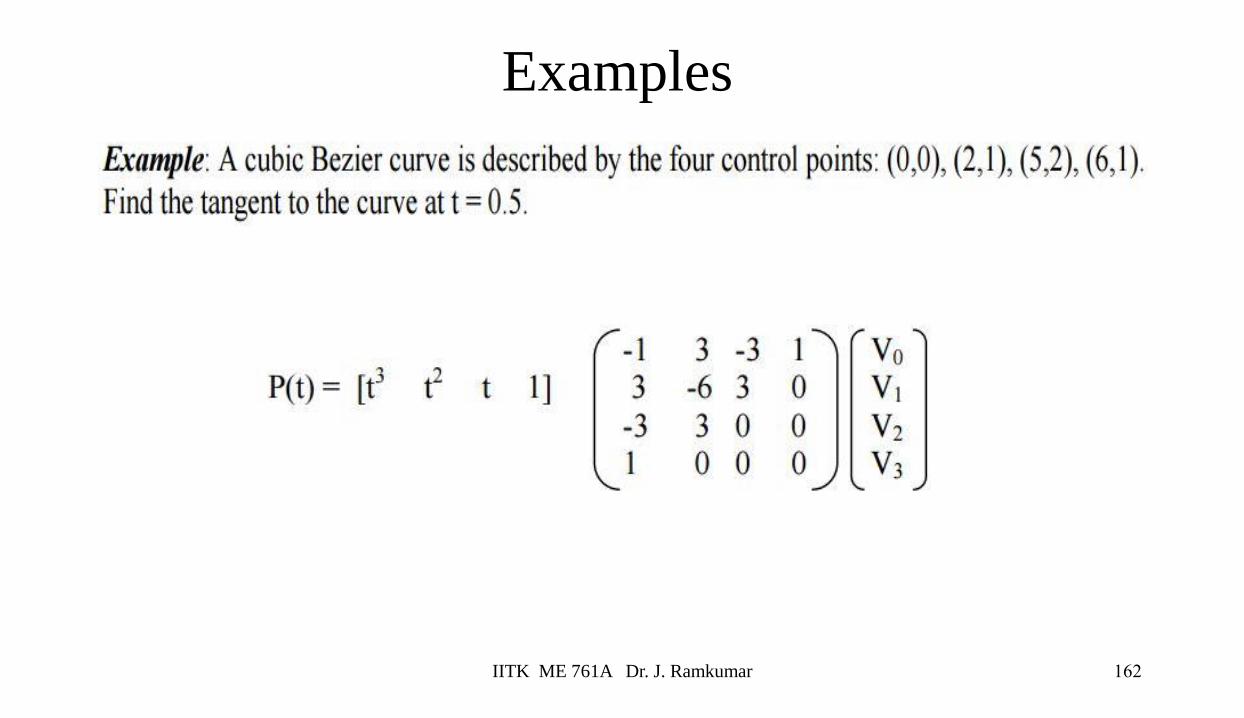
IITK ME 761A Dr. J. Ramkumar 162
Examples

IITK ME 761A Dr. J. Ramkumar 163
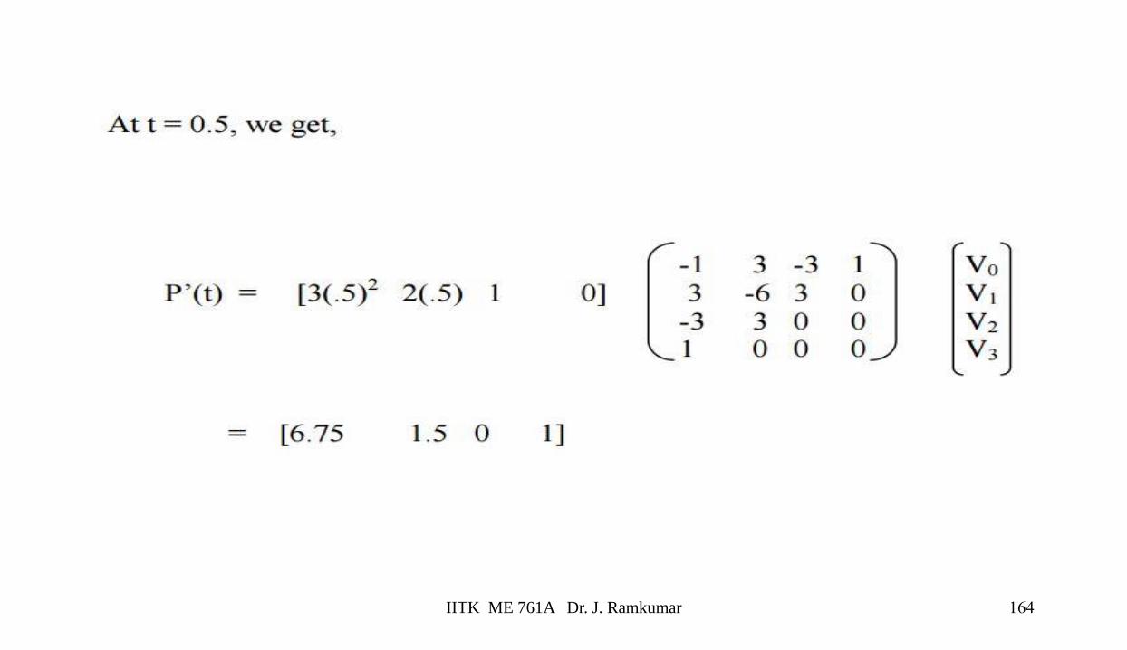
IITK ME 761A Dr. J. Ramkumar 164

Bezier Polynomial Function
ini
in ttini
ntB −−
−= )1.(.
)!(!
!)(
165IITK ME 761A Dr. J. Ramkumar
P(t)= σ𝑖=0𝑛 𝐶𝑖𝐵𝑖𝑛 (𝑡)
Ai is the control points (xi, yi)
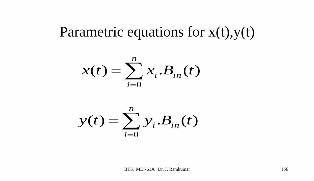
Parametric equations for x(t),y(t)
)(.)(0
tBxtx in
n
i
i=
=
)(.)(0
tByty in
n
i
i=
=
166IITK ME 761A Dr. J. Ramkumar
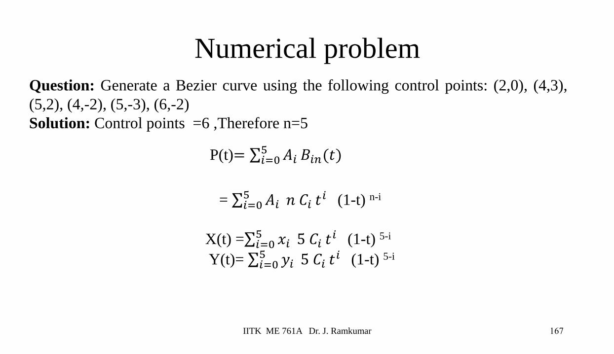
Numerical problem
IITK ME 761A Dr. J. Ramkumar 167
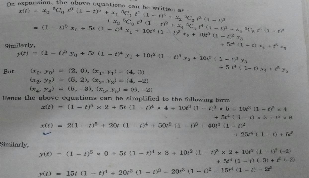
Question: Generate a Bezier curve using the following control points: (2,0), (4,3),
(5,2), (4,-2), (5,-3), (6,-2)
Solution: Control points =6 ,Therefore n=5
= σ𝑖=05 𝐴𝑖 𝑛 𝐶𝑖 𝑡
𝑖 (1-t) n-i
X(t) =σ𝑖=05 𝑥𝑖 5 𝐶𝑖 𝑡
𝑖 (1-t) 5-i
Y(t)= σ𝑖=05 𝑦𝑖 5 𝐶𝑖 𝑡
𝑖 (1-t) 5-i
P(t)= σ𝑖=05 𝐴𝑖 𝐵𝑖𝑛(𝑡)
IITK ME 761A Dr. J. Ramkumar 168
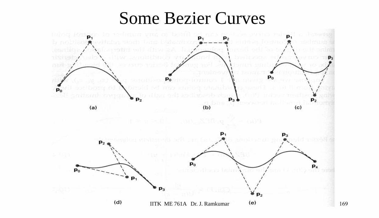
Some Bezier Curves
169IITK ME 761A Dr. J. Ramkumar
Bezier Curves - properties
• Not all of the control points are on the line
– Some just attract it towards themselves
• Points have “influence” over the course of the line
• “Influence” (attraction) is calculated from a polynomial expression
• (show demo applet)
170IITK ME 761A Dr. J. Ramkumar
1P
3P
2P
4P
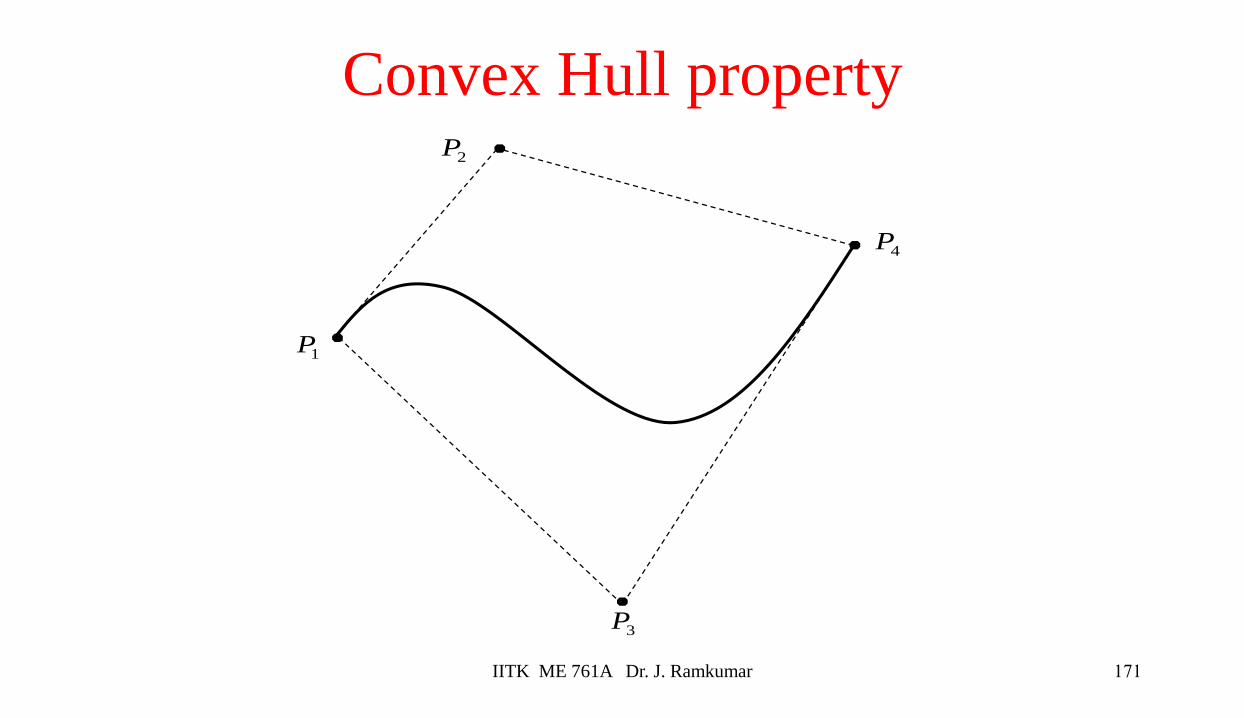
Convex Hull property
171IITK ME 761A Dr. J. Ramkumar
Bezier Curve Properties• The first and last control points are interpolated
• The tangent to the curve at the first control point is along the line joining the first and second control points
• The tangent at the last control point is along the line joining the second last and last control points
• The curve lies entirely within the convex hull of its control points– The Bernstein polynomials (the basis functions) sum to 1 and are everywhere positive
• They can be rendered in many ways– E.g.: Convert to line segments with a subdivision algorithm
172IITK ME 761A Dr. J. Ramkumar

Disadvantages
• The degree of the Bezier curve depends on the
number of control points.
• The Bezier curve lacks local control. Changing
the position of one control point affects the entire
curve.
173IITK ME 761A Dr. J. Ramkumar
Invariance• Translational invariance means that translating the control points
and then evaluating the curve is the same as evaluating and then translating the curve
• Rotational invariance means that rotating the control points and then evaluating the curve is the same as evaluating and then rotating the curve
• These properties are essential for parametric curves used in graphics
• It is easy to prove that Bezier curves, Hermite curves and everything else we will study are translation and rotation invariant
174IITK ME 761A Dr. J. Ramkumar
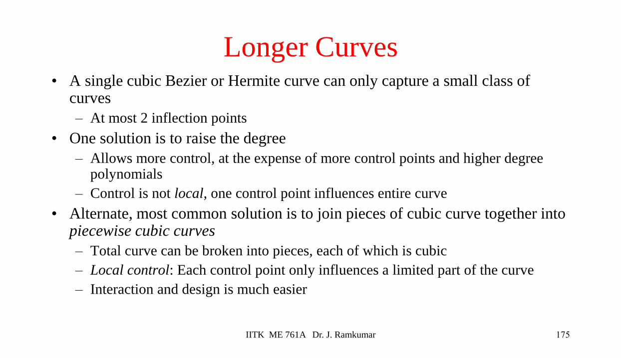
Longer Curves• A single cubic Bezier or Hermite curve can only capture a small class of
curves
– At most 2 inflection points
• One solution is to raise the degree
– Allows more control, at the expense of more control points and higher degree polynomials
– Control is not local, one control point influences entire curve
• Alternate, most common solution is to join pieces of cubic curve together into piecewise cubic curves
– Total curve can be broken into pieces, each of which is cubic
– Local control: Each control point only influences a limited part of the curve
– Interaction and design is much easier
175IITK ME 761A Dr. J. Ramkumar
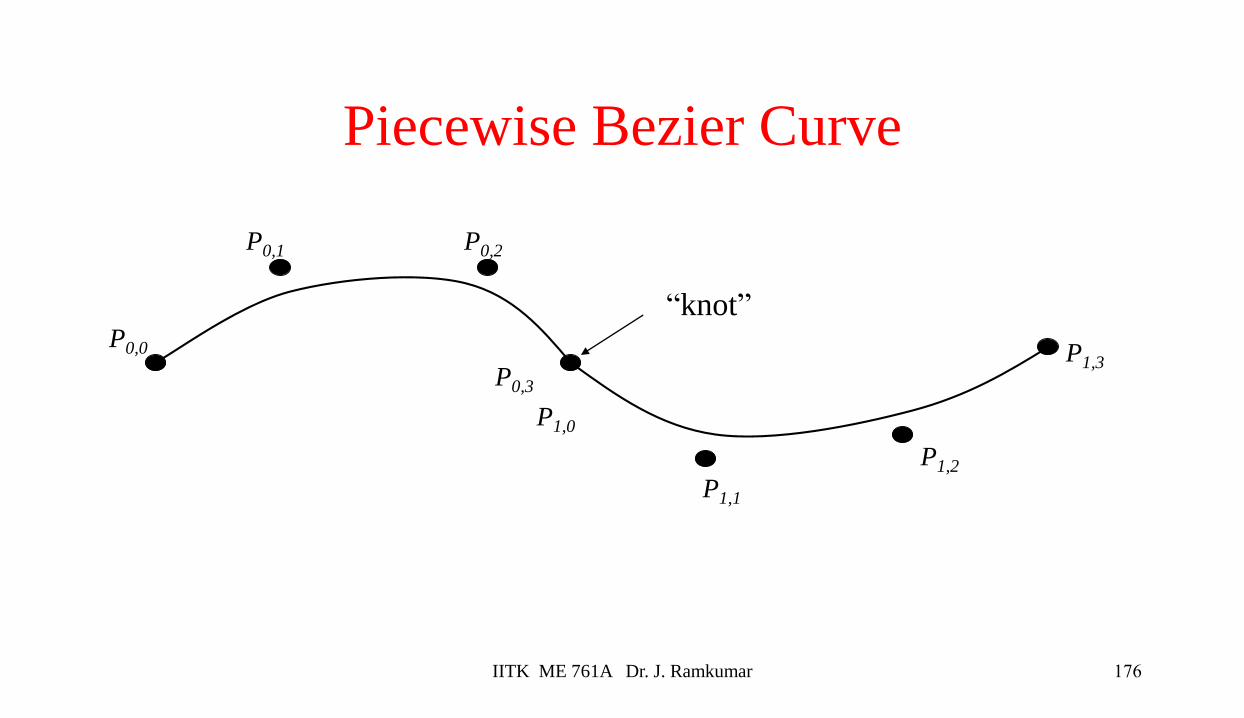
Piecewise Bezier Curve
“knot”P0,0
P0,1 P0,2
P0,3
P1,0
P1,1
P1,2
P1,3
176IITK ME 761A Dr. J. Ramkumar
Continuity• When two curves are joined, we typically want some degree of continuity
across the boundary (the knot)– C0, “C-zero”, point-wise continuous, curves share the same point where they join
– C1, “C-one”, continuous derivatives, curves share the same parametric derivatives where they join
– C2, “C-two”, continuous second derivatives, curves share the same parametric second derivatives where they join
– Higher orders possible
• Question: How do we ensure that two Hermite curves are C1 across a knot?
• Question: How do we ensure that two Bezier curves are C0, or C1, or C2
across a knot?
177IITK ME 761A Dr. J. Ramkumar
Achieving Continuity• For Hermite curves, the user specifies the derivatives, so C1 is achieved
simply by sharing points and derivatives across the knot
• For Bezier curves:
– They interpolate their endpoints, so C0 is achieved by sharing control points
– The parametric derivative is a constant multiple of the vector joining the first/last 2 control points
– So C1 is achieved by setting P0,3=P1,0=J, and making P0,2 and J and P1,1 collinear, with J-P0,2=P1,1-J
– C2 comes from further constraints on P0,1 and P1,2
178IITK ME 761A Dr. J. Ramkumar
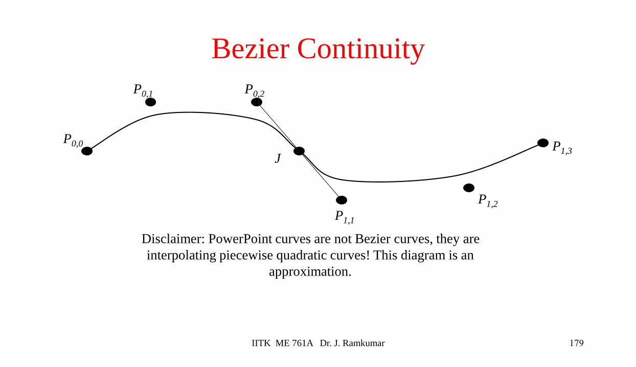
Bezier Continuity
P0,0
P0,1 P0,2
J
P1,1
P1,2
P1,3
Disclaimer: PowerPoint curves are not Bezier curves, they are
interpolating piecewise quadratic curves! This diagram is an
approximation.
179IITK ME 761A Dr. J. Ramkumar
Problem with Bezier Curves
• To make a long continuous curve with Bezier segments requires
using many segments
• Maintaining continuity requires constraints on the control point
positions
– The user cannot arbitrarily move control vertices and automatically
maintain continuity
– The constraints must be explicitly maintained
– It is not intuitive to have control points that are not free
180IITK ME 761A Dr. J. Ramkumar
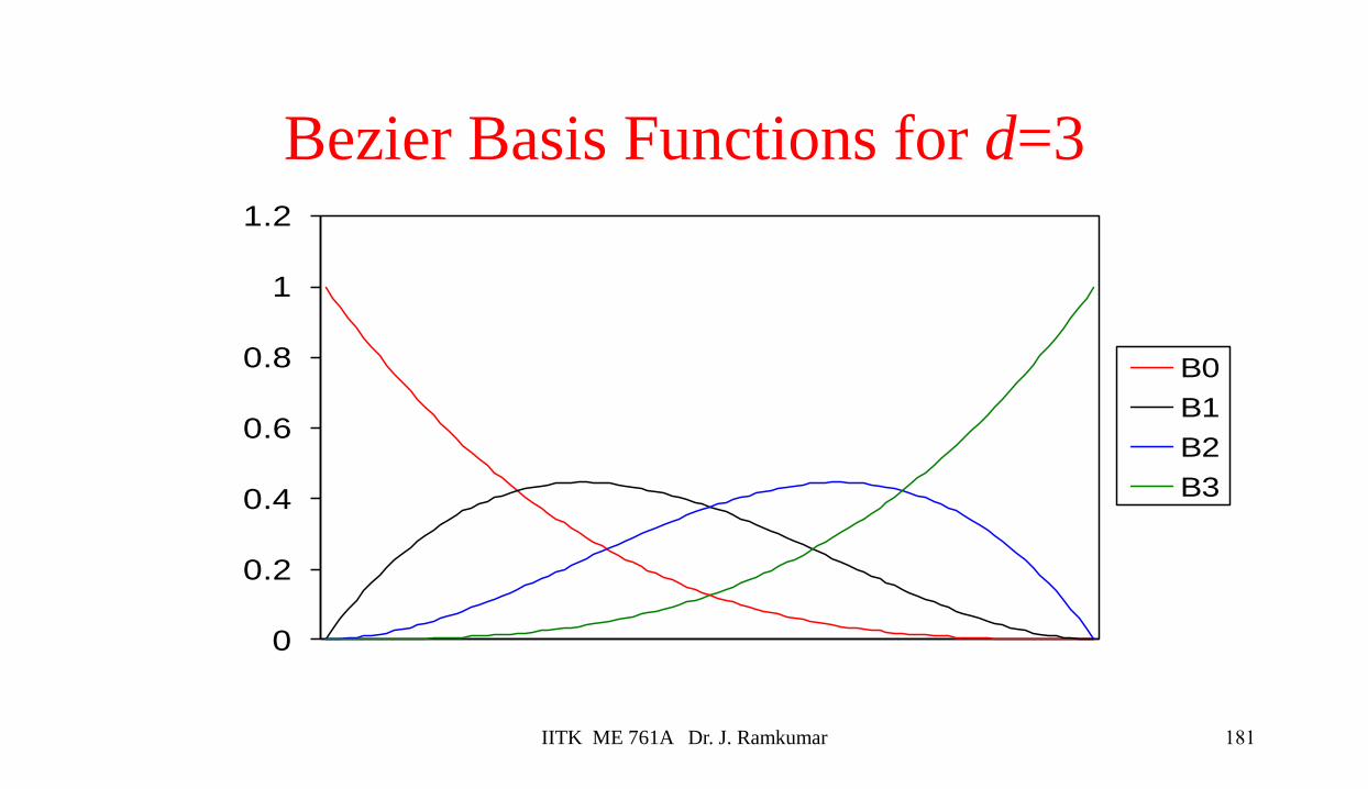
Bezier Basis Functions for d=3
0
0.2
0.4
0.6
0.8
1
1.2
B0
B1
B2
B3
181IITK ME 761A Dr. J. Ramkumar