Introduction to Climate Models:history and basic structure

Topics covered:

1. Introduction to climate models2. Brief history3. Physical parametrizations

Definition and a healthy philosophy regarding climate models

The climate System

Brief history of climate modelling• 1922: Lewis Fry Richardson

– basic equations and methodology of numerical weather prediction

• 1950: Charney, Fjørtoft and von Neumann (1950)– first numerical weather forecast (barotropic vorticity equation model)

• 1956: Norman Phillips– first general circulation experiment (two-layer, quasi-geostrophic hemispheric model)

• 1963: Smagorinsky, Manabe and collaborators at GFDL, USA– 9 level primitive equation model

• 1960s and 1970s: Other groups and their offshoots began work– University of California Los Angeles (UCLA), National Center for Atmospheric

Research (NCAR, Boulder, Colorado) and UK Meteorological Office

• 1990s: Atmospheric Model Intercomparison Project (AMIP)– Results from about 30 atmospheric models from around the world

• 2007: IPCC Forth Assessment Report– climate projections to 2100 from numerous coupled ocean-atmosphere-cryosphere

models.

How do they see our planet?

20 Ocean Levels

19 Atmospheric Levels

Met Office Unified Model level structure: more recent grids

HADLEY CENTRE CLIMATE MODELSHadCM21994

HadCM31998

HadGEM12003

Atmosphere 2.5 x 3.7519 levels

2.5 x 3.7519 levels

1.25 x 1.87538 levels

Ocean 2.5 x 3.7520 levels

1.25 x 1.2520 levels

1 x 140 levels

Flux adjust?Radiation

YesCO2 equiv

Noseparate ghg

Noseparate ghg

Sulphur cycleCarbon cycle

NoNo

YesNo

YesNo

ChemistryComputing

No1

No4

No40

HiGEM2 land-sea mask and bottom topographymodel has 1/3 degree resolution (“eddy permitting”)

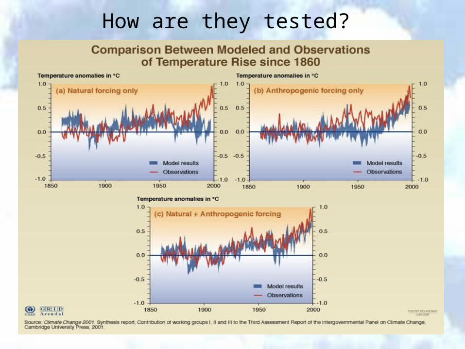
How are they tested?

Testing against Palaeo-data

ATMOSPHEREATMOSPHERE LANDLAND OCEANOCEAN ICEICE SULPHURSULPHUR CARBON CARBON CHEMISTRYCHEMISTRY

ATMOSPHEREATMOSPHERE LANDLAND OCEANOCEAN ICEICE SULPHURSULPHUR CARBON CARBON

ATMOSPHEREATMOSPHERE LANDLAND OCEANOCEAN ICEICE SULPHURSULPHUR

ATMOSPHEREATMOSPHERE LANDLAND OCEANOCEAN ICEICE

ATMOSPHEREATMOSPHERE LANDLAND OCEANOCEAN

ATMOSPHEREATMOSPHERE LANDLAND

ATMOSPHEREATMOSPHERE

19991999

19971997

19921992

19851985

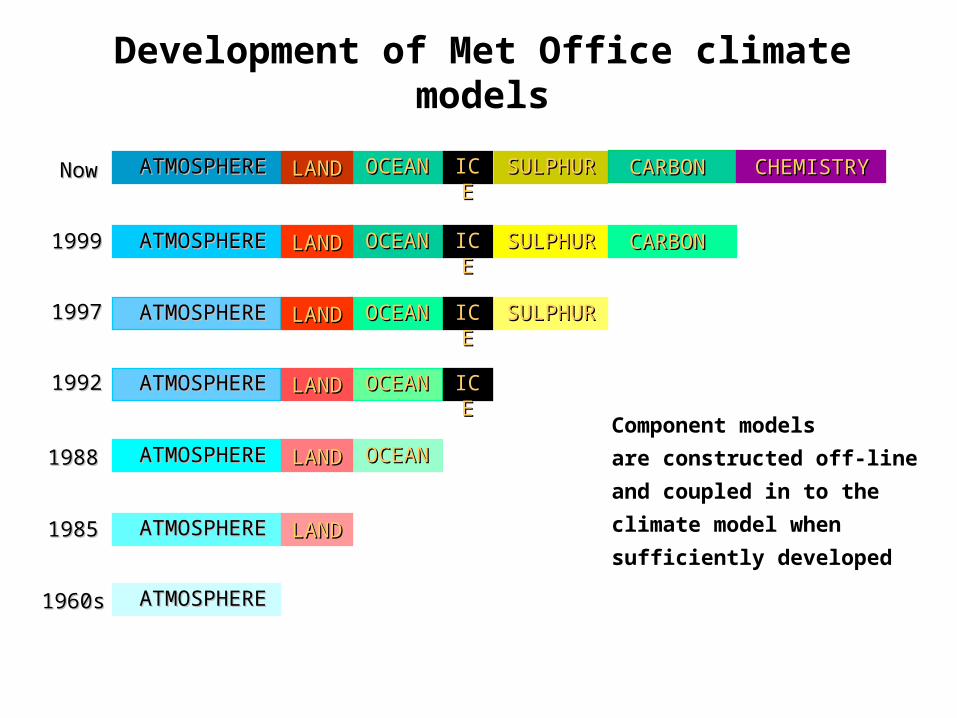
Development of Met Office climate models

Component models

are constructed off-line

and coupled in to the

climate model when

sufficiently developed

1960s1960s

NowNow

19881988

The horizontal and vertical resolutions of climate models need to be high enough to avoid numerical errors and to resolve the basic dynamical and transport processes

There is a trade-off between resolution and computing time, but model resolutions are increasing continually, as more computer power becomes available

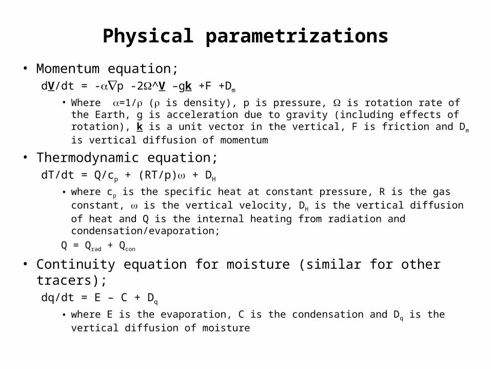
Physical parametrizations

• Momentum equation;dV/dt = -p -2^V –gk +F +Dm

• Where =1/ ( is density), p is pressure, is rotation rate of the Earth, g is acceleration due to gravity (including effects of rotation), k is a unit vector in the vertical, F is friction and Dm is vertical diffusion of momentum

• Thermodynamic equation;dT/dt = Q/cp + (RT/p) + DH

• where cp is the specific heat at constant pressure, R is the gas constant, is the vertical velocity, DH is the vertical diffusion of heat and Q is the internal heating from radiation and condensation/evaporation;

Q = Qrad + Qcon

• Continuity equation for moisture (similar for other tracers);dq/dt = E – C + Dq

• where E is the evaporation, C is the condensation and Dq is the vertical diffusion of moisture

Physical parametrizations in atmospheric models

• Processes that are not explicitly represented by the basic dynamical and thermodynamic variables in the basic equations (dynamics, continuity, thermodynamic, equation of state) on the grid of the model need to be included by parametrizations.

• There are three types of parametrization;

• Processes taking place on scales smaller than the grid-scale, which are therefore not explictly represented by the resolved motion;– Convection, boundary layer friction and turbulence, gravity wave drag

– All involve the vertical transport of momentum and most also involve the transport of heat, water substance and tracers (e.g. chemicals, aerosols)

• Processes that contribute to internal heating (non-adiabatic)– Radiative transfer and precipitation

– Both require the prediction of cloud cover

• Processes that involve variables additional to the basic model variables (e.g. land surface processes, carbon cycle, chemistry, aerosols, etc)

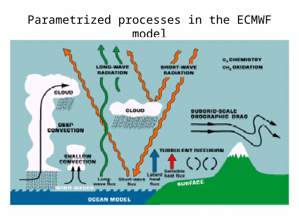
Parametrized processes in the ECMWF model

Atmospheric models include parametrizations for:

• cloud formation, microphysics and precipitation

• radiative transfer (both solar and thermal)

• dry and moist convection (and transport of tracers)

• surface exchanges and land surface processes

• drag processes (e.g. boundary layer, gravity waves)

• aerosols, chemistry, carbon cycle

Clouds and precipitation• GCMs cannot resolve clouds, but a knowledge of their amount and properties is important for the calculation of radiation fields and precipitation

• A GCM therefore needs a cloud parametrization. These have evolved in time with increasing complexity:

• Earliest (and simplest) cloud parametrization

• cloud amount = 0 if grid box is unsaturated

• cloud amount = 1 if grid box saturated (and excess humidity is rained out)

• Diagnostic schemes

• cloud amount is diagnosed from the model variables

• Prognostic schemes

• cloud amount is a prognostic variable, with tendency terms that enable the changes in cloud amount to be calculated (from new parametrizations…)

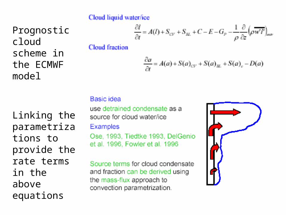
Prognostic cloud scheme in the ECMWF model

Linking the parametrizations to provide the rate terms in the above equations

Radiation

Radiative transfer: clouds

• earliest schemes used-ray tracing in shortwave and emissivity approximation in longwave

• cloud radiative properties were fixed

• no treatment of aerosols

• modern schemes use the “two-stream equations” which enable scattering to be included as well as calculation of radiative properties of clouds and aerosols

• The effect of particle size, phase (whether water or ice) and shape (ice crystals) can then be parametrized

• important for investigating the indirect effect of aerosols on cloud radiative properties

Convection

• The first convection schemes simply adjusted the temperature profile to remove super-adiabatic layers

• Most contemporary convection schemes use a mass-flux approach, with buoyant plumes entraining and detraining to reach different levels.

• Yanai et al. (1973)

• Arakawa and Scubert (1974)

• Gregory and Rowntree (1990)

• Important processes to be included are the effects of saturated downdraughts and momentum transport

• e.g. Gregory, Kershaw and Inness (1997)

Convection scheme

Schematic of an ensemble of cumulus clouds.

From Yanai et al. (1973)

Cloud mass fluxes.

denotes the entrainment of environmental air into the cloud

denotes the detrainment of cloud air into the environment

MC is the cloud mass flux

From Yanai et al. (1973)

Surface processes

• Surface schemes are needed to calculate the fluxes of heat, moisture and momentum between the surface and atmosphere and to calculate surface temperature and other variables

• Over the oceans, the schemes are quite simple

• Over land, models now contain quite detailed representations of evaporation, interception and vertical transfers of heat and moisture in the soil

• For example, MOSES I (in the Met Office Unified Model) includes a model of stomatal control of evaporation

• MOSES 2 also explicitly treats subgrid patchiness of the landscape with a tile scheme

Surface Hydrology in Met Office

Surface Exchange Scheme

(MOSES)

Representation of orography;the importance of resolution

The upper figure shows the surface orography over North America at a resolution of 480km, as in a low resolution climate model.

The lower figure shows the same field at a resolution of 60km, as in a weather forecasting model.

Remember that orographic processes are highly non-linear.

Orographic processes

• The effect of details of the surface orography that are not resolved by the model’s grid must be parametrized

• Processes that are known to be important include low level flow blocking and gravity wave drag

• The sub-gridscale variability of the orography is used to drive the parametrizations

Mean and standard deviation of orographic heights at two resolutions

NWP model: 60km

Mean: explicitly

resolved by the model

Standard deviation: used to

drive the parametrizations

Climate model: 250km

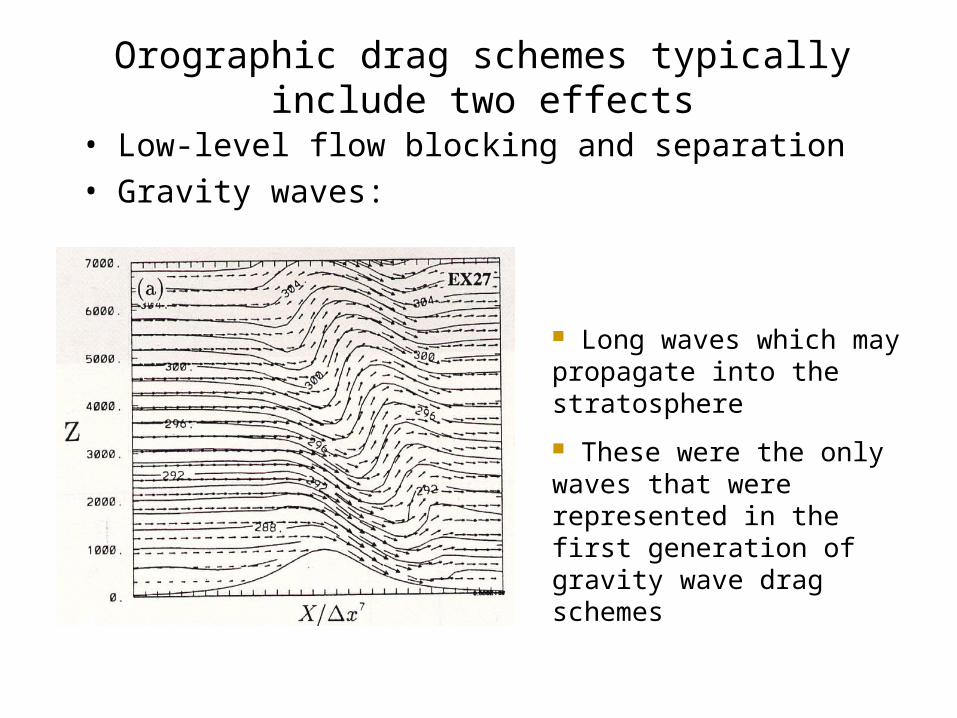
Orographic drag schemes typically include two effects

• Low-level flow blocking and separation

• Gravity waves:

Long waves which may propagate into the stratosphere

These were the only waves that were represented in the first generation of gravity wave drag schemes

Aerosols: Saharan dust

Further reading

• Books;

– Washington, W.M. and Parkinson, C.L., 1986. An introduction to three dimensional climate modeling. Oxford University Press

– Trenberth, K.E.,1995. Climate system modeling. Cambridge University Press

– Randall, D.A. 2000. General circulation model development. Academic Press

– Houghton, J.T. et al., 2001. Climate change 2001; the scientific basis. Cambridge University Press. (Working Group 1 contribution to the IPCC Third Assessment )

• Web pages;

– ECMWF seminars: http://www.ecmwf.int/newsevents/training/meteorological_presentations/

– AMIP: http://www-pcmdi.llnl.gov/amip/

– GFDL: http://www.gfdl.gov/

– NCAR: http://www.ncar.ucar.edu/ncar/

– GISS: http://www.giss.nasa.gov/research/modeling/

– Met Office: http://www.metoffice.com