Embed Size (px)
Citation preview
INTRODUCTION TO GEODETIC ASTRONOMY
D. B. THOMSON
December 1981
TECHNICAL REPORT NO. 217
LECTURE NOTES49
PREFACE
In order to make our extensive series of lecture notes more readily available, we have scanned the old master copies and produced electronic versions in Portable Document Format. The quality of the images varies depending on the quality of the originals. Inthis version, images have been converted to searchable text.
INTRODUCTION TO GEODETIC ASTRONOMY
Donald B. Thomson
Department of Geodesy and Geomatics Engineering University of New Brunswick
P.O. Box 4400 Fredericton, N.B.
Canada E3B SA3
September 1978 Reprinted with Corrections and Updates December 1981
Latest Reprinting January 1997
PREFACE
These notes have been written for undergraduate students
in Surveying Engineering at the University of New Brunswick. The
overall objective is the development of a set of practical models
for the determination of astronomic azimuth, latitude and longitude
that utilize observations made to celestial objects. It should be
noted here that the emphasis in these notes is placed on the so
called second-order geodetic astronomy. This fact is reflected
in the treatment of some of the subject matter. To facilitate
the development of models, several major topics are covered, namely
celestial coordinate systems and their relationships with terrestrial
coordinate systems, variations in the celestial coordinates of a
celestial body, time systems, timekeeping, and time dissemination.
Finally, the reader should be aware of the fact that much
of the information contained herein has been extracted from three
primary references, namely Mueller [1969], Robbins [1976], and
Krakiwsky and Wells [1971]. These, and several other's, are referenced
extensively throughout these notes.
D.B. Thomson.
ii
TABLE OF CONTENTS
PREFACE ••••
LIST OF TABLES
LIST OF FIGURES
1. INTRODUCTION • • • • • 1.1 Basic Definitions
2. CELESTIAL COORDINAT~ SYSTEMS
2.1 2.2
The Celestial Sphere • • • • • Celestial Coordinate Systems • •••••• 2.2.1 Horizon System ••••••••••••. 2.2.2 Hour Angle System ••••••••• 2.2.3 Right Ascension System. • ••• 2.2.4 Ecliptic Sys tem • • • • 2.2.5 Summary • • • • • • • •
Page
ii
v
vi
1 2
2.3 Transformations Amongst Celestial Coordinate Systems • 2.3.1 Horizon - Hour Angle •••••
14
14 20 20 23 26 29 32 34 36 42 44 47 47 50 59 61 64
2.4
2.3.2 Hour Angle - Right Ascension • 2.3.3 Right Ascension - Ecliptic •• 2.3.4 Summary ••••••• Special Star Positions 2.4.1 Rising and Setting of Stars 2.4.2 Culmination (Transit) 2.4.3 Prime Vertical Crossing. 2.4.4 Elongation •••••••
3. TIME SYSTEMS
3.1 Sidereal Time ••• • • • 3.2 Universal (Solar) Time •••
3.2.1 Standard(Zone) Time 3.3 Relationships Between Sidereal and Solar Time Epochs
and Intervals •• • • • • • 3.4 Irregularities of Rotational Time Systems • 3.5 Atomic Time System. • • • •
67 75 80
80 93 93
4. TIME DISSEMINATION, TIME-KEEPING, TIME RECORDING . . . . 95
4.1 Time Dissemination • • • •••• 4.2 Time-Keeping and Recording. 4.3 Time Observations •••••
5. STAR CATALOGUES AND EPHEMERIDES 5.1 Star Catalogues .5.2 Ephemerides and Almanacs ••
iii
. . .
. . •. 95 99
• • • 100
• • • • 106 • 108
6. VARIATIONS IN CELESTIAL COORDINATES· ••••••••••
6.1 Precession, Nutation, and Proper Motion· 6.2 Annual Aberration and Parallax •••••••••• 6.3 Diurnal Aberration, Geocentric Parallax, and
Astronomic f'1.~(~~'~:.ton • • •• •••• 6.4 Polar Motion • • • • • • • • • • • • •
Page
117
118 127
134 138
7. DETERMINATION OF ASTRONOMIC AZIMUTH . . . . . . . . 147
7.1 Azimuth by Star Hour Angles •• 7.2 Azimuth by Star Altitudes
8. DETERMINATION OF ASTRONOMIC LATITUDE •
8.1 Latitude by Meridian Zenith Distances •• 8.2 Latitude by Polaris at any Hour Angle ••
9. DETERMINATION OF ASTRONOMIC LONGITUDE •••
9.1 Longitude by Meridian Transit Times· •
REFERENCES • • • • • • • • • • • • • • • • •
APPENDIX A Review of Spherical Trigonometry ••
APPENDIX B Canadian Time Zones
148 154
163
164 165
170
• 172
• 175
176
183
APPENDIX C Excerpt from the Fourth Fundamental Catalogue (FK4) . . • . . • . . • . • .,. . • ... . . 184
APPENDIX D Excerpt from Apparent Places of Fundamental Stars •• • • • • • • • • • • • • • • • • • • • • • • 186
iv
LIST OF TABLES
Table 2-1 Celestial Coordinate Systems [Mueller, 1969] . • 33
Table 2-2 Cartesian Celestial Coordinate Systems [Mueller, 1969] 33
Table 2-3 Transformations Among Celestial Coordinate Systems
[Krakiwsky and Wells, 1978J .
Table 6-1 Description of Terms • .
Table 7-1 Azimuth by Hour Angle:Random Errors in Latitude 60 0
[Robbins, 1976]
Table 7-2 Azimuth by Altitude: Random Errors in Latitude 60 0
[Robbins, 1976] ••••••
v
49
133
155
158
LIST OF FIGURES
Figure 1-1 Biaxial Ellipsoid • . • • • • 4
Figure 1-2 Geodetic Latitude, Longitude, and Ellipsoidal Height 5
Figure 1-3 Orthometric Height
Figure 1-4 Astronomic Latitude (~) and Longitude (A)
6
8
Figure 1-5 Geoid Height & Terrain Deflection of the Vertical • .. 9
Figure 1-6 Components of the Deflection of the Vertical 10
Figure 1-7 Geodetic Azimuth • •
Figure 1-8 Astronomic Azimuth
Figure 2-1 Cele,stial Sphere ••
Figure 2-2 Astrono~ic Triangle. .
Figure 2-3 Sun's Apparent Motion
Figure 2-4 Horizon System . . . . Figure 2-5 Horizon System
Figure 2-6 Hour Angle System.
Figure 2-7 Hour Angle System
Figure 2-8 Right Ascension System
Figure 2-9 Right Ascension System
Figure 2-10 Ecliptic System.
Figure 2-11 Ecliptic System.
Figure 2-12 Astronomic Triangle •
Figure 2-13 Local Sidereal Time •
. . . . . . . . . . . .
vi
. . . . .
. .
. .
. .
. .
12
13
16
17
19
21
22
24
25
27
28
30
31
35
37
List of Figures Cont'd
Figure 2-14
Figure 2-15
Horizon and Hour Angle System Transformations •
Horizon and Hour Angle Systems • • • • • • •
Figure 2-16 Hour Angle - Right Ascension Systems •
Figure 2-17 Right Ascension-Ecliptic Systems • •
Figure 2-18 Celestial Coordinate System Relationships [Krakiwsky
and We.lls, 1971] •.
Figure 2-19 Circumpolar and Equatorial Stars •
Figure 2-20 Declination for Visibility • •
Figure 2-21 Rising and Setting of a Star • •
Figure 2-22
Figure 2-23
Hour Angles of a Star's Rise and Set
Rising and Setting of a Star
Figure 2-24 Azimuths of a Star's Rise and Set.
Figure 2-25 Culmination (Transit) • •
Figure 2-26 Prime Vertical Crossing •
Figure 2-27 Elongation. •
Figure 3-1 Sidereal Time Epochs •
. . .. . . . . .
Figure 3-2 Equation of Equinoxes (OhUT , 1966) [Mueller, 1969]
Figure 3-3
Figure 3-4
Figure 3-5
Figure 3,...6
Figure 3-7
Figure 3-8
Figure 3-9
Sidereal Time and Longitude
Universal and Sideral Times fAA, 1981] •
Universal (Solar) Time • • • . • • • • •
Equation of Time (OhUT , 1966) [Mueller, 1969] •
Solar Time and Longitude • • •
Standard (Zone) Time [Mueller, 1969]
Relationships Between Sidereal and Universal Time Epochs
vii
39
41
43
45
48
51
52
54
55
57
58
60
62
65
70
71
72
74
76
78
79
81
83
List of Figures Cont'd
Figure 3-10 Sun - February. 1978 [SALS~-.i98ir. • •
Figure 3-11 Mutual Conversion of Intervals of Solar and
.Siderea1 Time [SALS, 19811 •
Figure 3-12a Universal and Sidereal Times, ·1981 [AA,1981J •
Figure 3-12b Universal and Sidereal Times, 1981 cont'd.
[AA, 1981] • • • • • • • • •
Figure 3-12c Universal and Sidereal Times, 1981 cont'd.
Figure 4-1 Code for the Transmission of DUT1
86
87
88
89
90
97
Figure 4-2 ,:·pating. of Events in the Vicinity of A Leap ~econd... 98
Figure 5-1 Universal and Sidereal Times, 1981 [AA 1981' ,. J · · · · 109
Figure 5-2 Bright Stars, 1981.0
[AA,··r9S1] . . . . . . . . . . · · . 110 .,- .
Figure 5-3 Bright Stars, 1981.0 cont'd. [AA" 1281] . . III
. /
Figure 5-4 Sun - February, 1981 [SALS ,1981 L .. · · . . .. 113
Figure 5-5a Right Ascension of Stars, 1981 [BALS, 1981 ] . 114
Figure 5-5b Declination of Stars t 1981, [SALS, 1981].· · 115
Figure 5-6 Pole Star Table, 1981 [SALS, 1-981] .' · · · · 116
Figure 6-1 Variations of the Right Ascension System • 119
Figure 6-2 Motion of the Celestial Pole . . . · · · . . . .. 121
Figure 6-3 Mean Celestial Coordinate Systems . · . . · . · · · · 123
Figure 6-4 True and Mean Celestial coordinate Systems 126
Figure 6-5 Aberration . . 0 0 . 0 0 0 0 0 0 0 · · · . 129
Figure 6.;;.;6 Annual (Stellar) Parallax •• 0 . 0 · 0 0 0 130
Figure 6-7 Position Updating M.Co T to A.Po T 0 0 0 0 0 132 0
Figure 6-8 Geocentric Parallax . . . . 0 0 . . · . . · 0 0 0 0 0 136
viii
List of Figures cont'd
Figure 6-9
Figure 6-10
Astronomic Refraction • • • • • • • • • • .
Observed to Apparent Place
137
139
Figure 6-11 Transformation of Apparent Place 141
Figure 6-12 Transformation from Instantaneous to Average Terrestrial
Figure 6-13
Figure 6-:-14
Figure 7-1
Figure 7-1
Figure 7-2
System • • • •
Celestial Coordinate Systems and Position Updating
[Krakiwsky, Wells, 1971] • . •••
Coordinate Systems Used in Geodesy • ••••
Azimuth by the Hour Angle of Polaris [Mueller, 1969]
Cont'd • •
Azimuth by the Sun's Altitude •••••••••••.•
ix
143
145
146
152
153
159

1. INTRODUCTION
Astronomy is defined as [Morris~ 19751 "The scientific
study of the universe beyond the earth~ especially the observation,
calculation, and theoretical interpretation of the positions, dimensions,
distribution~ motion, composition, and evolution of celestial bodies and
phenomena". Astronomy is the oldest of the natural sciences dating back to
ancient Chinese and Babylonian civilizations. Prior to 1609, when the
telescope was invented, the naked eye was used for measurements.
Geodetic astronomy, on the other hand, is described as [Mueller,
1969] the art and science for determining, by astronomical observations,
the positions of points on the earth and the azimuths of the geodetic lines
connecting such points. When referring to its use in surveying, the terms
practical or positional astronomy are often used. The fundamental concepts
and basic principles of "spherical astronomy", which is the basis for geodetic
astronomy, were developed principally by the Greeks, and were well established
by the 2nd century A.D.
The treatment of geodetic astronomy in these notes is aimed at
the needs of undergraduate surveying engineers. To emphasise the needs, listed
below are ten reasons for studying this subject matter:
(i) a knowledge of celestial coordinate systems, transformations
amongst them, and variations in each of them;
(ii) celestial coordinate systems define the "linkll between satellite
and terrestrial coordinate systems;
(iii) the concepts of time for geodetic purposes are developed;
(iv) tidal studies require a knowledge of geodetic astronomy;
1
2
(v) when dealing with new technologies (e.g. inertial survey systems)
an understanding of the local astronomic coordinate system is
essential;
(vi) astronomic coordinates of terrain points, which are expressed
in a "natural" coordinate system, are important when studying
3-D terrestrial networks;
(vii) astrondmically determined azimuths provide orientation for
terrestrial networks;
(viii) the determination of astrogeodetic deflections of the vertical
are useful for geoid determination, which in turn may be required
for the rigorous treatment of terrestrial observations such as
distances, directions, and angles;
(ix) geodetic astronomy is useful for the determination of the origin
and orientation of independent surveys in remote regions;
(x) geodetic astronomy is essential for.the demarcation of astro
nomically defined boundaries.
1.1 Basic definitions
In our daily work as surveyors, we commonly deal with three different
surfaces when referring to the figure of the earth: (i) the terrain, (ii)
an ellipsoid, and (iii) the geoid.
The physical surface of the earth is one that is extremely difficult
to model analytically. It is common practice to do survey computations on a
less complex and modelable surface. The terrain is, of course, that surface
on or from which all terrestrially based observations are made.
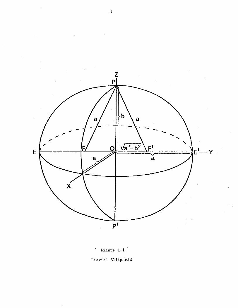
The most common figure of the earth in use, since it best approxi
mates the earth's size and shape is a biaxial ellipsoid. It is a purely
3
mathematical figure, defined by the parameters a (semi-major axis) b (semi
minor axis) or a and f (flattening), where f=(a-b)/a (Figure 1-1). This figure
is commonly referred to as a "reference ellipsoid", but one should note that
there are many of these for the whole earth or parts thereof. The use of a
biaxial ellipsoid gives rise to the use of curvilinear geodetic coordinates -
<P (latitude), A (longitude) ,and h (ellipsoidal height) (Figure 1-2). Obviously,
since this ellipsoid is a "mathematical" figure of the earth, its position and
orientation within the earth body is chosen at will. Conventionally, it has
been positioned non-geocentrically, but the trend is now to have a geocentric
datum (reference ellipsoid). Conventional orientation is to have parallel~m of
the tertiary (:Z) axis with the mean rotation axis of the earth, and parallelism'
of the primary (X) axis with the plane of the Greenwich Mean Astronomic
Mer:t.dian.
Equipotential surfaces (Figure 1-3), of which there are an infinite
number for the earth, can be represented mathematically. They account for the
physical properties of the earth such as mass, mass distribution, and rotation,
and are "real" or physical surfaces of the earth. The common equipotential
surface used is the geoid, defined as [Mueller, 1969] " t hat equipotential
surface that most nearly coincides with the undisturbed mean surface of the
oceans". Associated with these equipotential surfaces is the plumhline
(Figure 1~3). It is a line of force that is everywhere normal to the equipo
tential surfaces; thus, it is a spatial curve.
We now turn to definitions of some fundamental quantities in geodetic
astronomy namely, the astronomic latitude (4)), astronomic longitude (A), and
orthometricheight (H). These quantities are sometimes referred to as
"natural" coordinates, since, by definition, they are given in terms of the
·4
z p
pi
Figure 1-1
Biaxial Ellipsoid
5
..
z. ELLIPSOIDAL NORMAL
~~-r------~~Y o·
(A=90)
Figure 1-2
Geodetic Latitude,Longitude, and r.llipsoida1Height ,
GEOID
6
PLUMBLINE
EQUIPOTENTIAL SURFACES
TERRAIN
r ELL~
Figure 1-3
Orthometric lIeieht

7
"real" (physical) properties of the earth.
Astronomic latitude (~) is defined as the angle between the
astronomic normal (gravity vertical) (tangent to the plumb1ine a.t the point
of interest) and the plane of the instantaneous equator measured in the
astronomic meridian plane (Figure 1 ... 4). Astronomic longitude (/I.) is the
angle between the Greenwich Mean Astronomic Meridian and the astronomic
meridian plane measured in the plane of the instantaneous equator (Figure
1 ... 4).
The orthometr1c height (H), is the height of the point of interest
.above the geoid, measured along the plumbline, as obtained from spirit
leveling and en route gravity observations (Figure 1-3). Finally, after some
reductions of ~ and A for polar motion and plumb line curvature, one obtains .
the "reduced" astronomic coordinates (~, A, H) referring to the geoid and the
mean rotation axis of the earth (more will be said about this last point in
these notes).
We are now in a position to examine the relationship between the
Geodetic and Astronomic coordinates. This is an important step for surveyors.
Observations are made in the natural system; astronomic coordinates are expressed
in the same natural system; therefore, to use this information for computations
in a geodetic system, the relationships must be known.
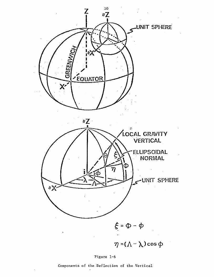
The astro-geodetic (relative) deflection of the vertical (a) at a
point is the angle between the astronomic normal at that point and the normal
to the reference ellipsoid at the corresponding point (the point may be on
the terrain (at) or on the geoid{s ) (Figure 1-5). g
e is normally split into
t~o components, ~ - meridian and n - prime vertical (Figure 1-6). Mathema-
tically, the components are given by
~ = ~- !fl, n = (A-A) cos !fl,
(1-1)
(1-2)
8
TRUE. - Z'T' ROTATION 'AXIS INSTANTANEOUS
POLE
PlUMBliNE GRAVITY VERTICAL
Figu.re 1-4
Astronomic Latitu.de (4)) and Longitude (A)
ELLIPSOIDAL NORMAL-~
9
PLUMBLINE
EQUIPOTENTIAL ~~~-- SURFACE' - --
"'ERRA.IN
GEOID
ELLIPSOID
Fieure 1-5
Geoid Ueieht & Terrain Deflection of the Vertical
z
liZ 0
10
liZ
ELLIPSOIDAL NORMAL
UNIT SPHERE
7J =(1\. - 'A.) cos <P
Figure 1-6
Components of the Deflection of the Vertical
11
which yields the geodetic-astronomic coordinate relationships we were seeking.
The geoida1 height (N) is the distance between the geoid and a
reference ellipsoid, measured along an ellipsoidal normal (Figure 1-5).
Mathematically, N is given by (with an error of less than 1mm) tie1sianen
and Moritz, 1967]
N = h-H. (1-3)
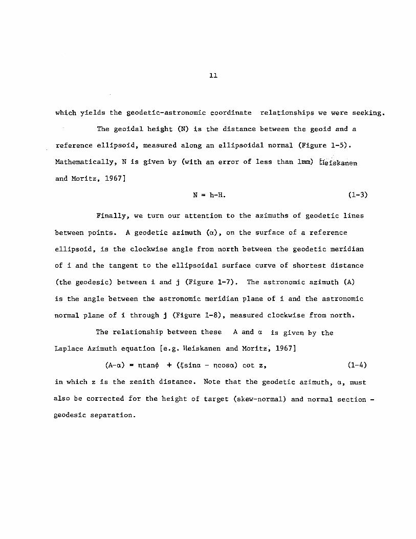
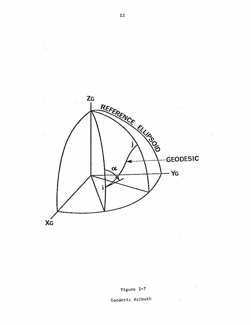
Finally, we turn our attention to the azimuths of geodetic lines
between points. A geodetic azimuth (a), on the surface of a reference
ellipsoid, is the clockwise angle from north between the geodetic meridian
of i and the tangent to the ellipsoidal surface curve of shortest distance
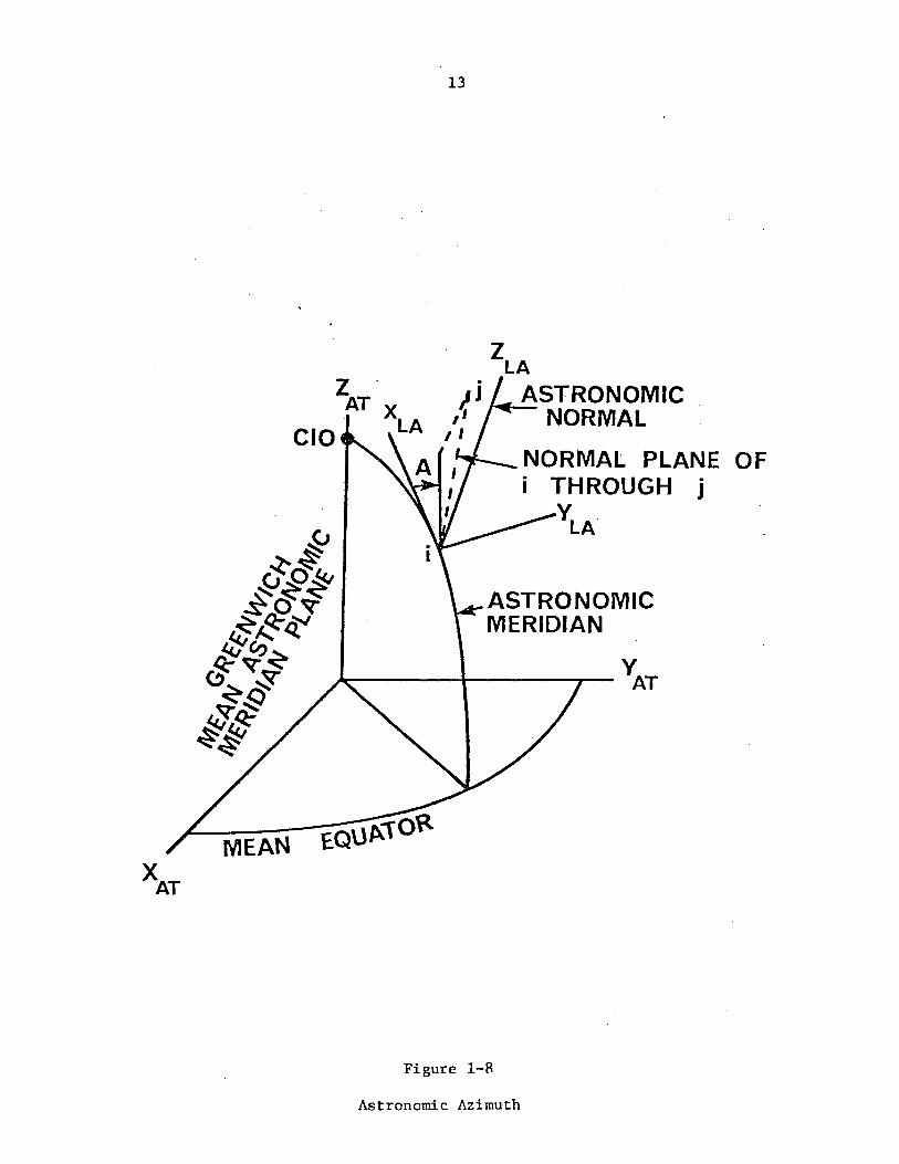
(the geodesic) between i and j (Figure 1-7). The astronomic azimuth (A)
is the angle between the astronomic meridian plane of i and the astronomic
normal plane of i through j (Figure 1-8), measured clockwise from north.
The relationship between these A and a is given by the
Laplace Azimuth equation [e.g. Heiskanen and Moritz~ 1967]
(A-a) = ntan~ + (~sina - ncosa) cot z, (1-4)
in which z is the zenith distance. Note that the geodetic azimuth, a, must
also be corrected for the height of target (skew-normal) and normal section -
geodesic separation.
XG
12
ZG
#4-----'--4- GEODES I C
kc::--t----=~-----l~-l-- YG
Figure 1-7
Geodetic Azimuth
13
Z AT X
CIO LA
ZLA
~ASTRONOMIC . NORMAL
NORMAL PLANE OF THROUGH j VLA,
ASTRONOMIC' MERIDIAN
Figure 1-R
Astronomic Azimuth
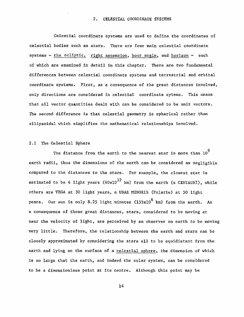
2. CELESTIAL COORDINATE SYSTEMS
Celestial coordinate systems are used to define the coordinates of
celestial bodies such as stars. There are four main celestial coordinate
systems - the ecliptic,'rightascelision, hour angle, and horizon - each
of which are examined in detail in this chapter. There are two fundamental
differences between celestial coordinate systems and terrestrial and orbital
coordinate systems. First, as'a consequence of the great distances involved,
only directions are considered in celestial coordinate sytems. This means
that all vector quantities dealt with can be considered to be unit vectors.
The second difference is that celestial geometry is spherical rather than
ellipsoidal which simplifies the mathematical relationships involved.
2.1 The Celestial Sphere
The distance from the earth to the nearest star is more than 109
earth radii, thus the dimensions of the earth can be considered as negligible
compared to the distances to the stars. For example, the closest star is
estimated to be 4 light years (40xl012 km) from the earth (a CENTAURI), while "
others are VEGA at 30 light years, a USAE MINORIS (Polaris) at 50 light
years. Our sun is only 8.25 light minutes (155xl06 km) from the earth. As
a consequence of those great distances, stars, considered to be moving at
near the velocity of light, are perceived by an observer on earth to be moving
very little. Therefore, the relationship between the earth and stars can be
closely approximated by considering the stars all to be equidistant from the
earth and lying on the surface of a celestial sphere, the dimension of which
is so large that the earth, and indeed the solar system, can be considered
to be a dimensionless point at its centre. Although this point may be
14
15
considered dimensionless, relationships between directions on the earth
and in the solar system can be extended to the· celestial sphere.
The instantaneous rotation axis of the earth intersects the
celestial sphere at the north and south celestial poles (NCP and SCP
respectively) (Figure 2-1). The earth's equitorial plane extented outwara
intersects the celestial sphere at the celestial equator (Figure 2-1).
The vertical (local-astronomic normal) intersects the celestial sphere at
a point above the observer, the zenith, and a point beneath. the observer,
the nadir (Figure 2-1). A great circle containing the poles, and is thus
perpendicular to the celestial equator, is called an hour circle (Figure 2-1).
The observer's vertical plane, containing the poles, is the hour circle through
the zenith and is the observer's 'celestial meridian (~igure 2-1). A small
circle parallel to the celestial equator is called a celestial parallel. Another
very important plane is that which is normal to the local astronomic vertical
and contains the observer (centre of the celestial sphere); it is the
celestial horizon (Figure 2-1). The plane normal to the horizon passing
through the zenith is the vertical plane. A small circle parallel to the
celestial horizon is called an almucantar~ The vertical plane normal to the
celestial meridian is called the prime vertical. The intersection points of
the prime vertical and the celestial horizon are the ~ and west points.
Due to the rotation of the earth, the zenith (nadir), vertical
planes, almucantars, the celestial horizon and meridian continuously change
their positions on the celestial sphere, the effects of which will be studied
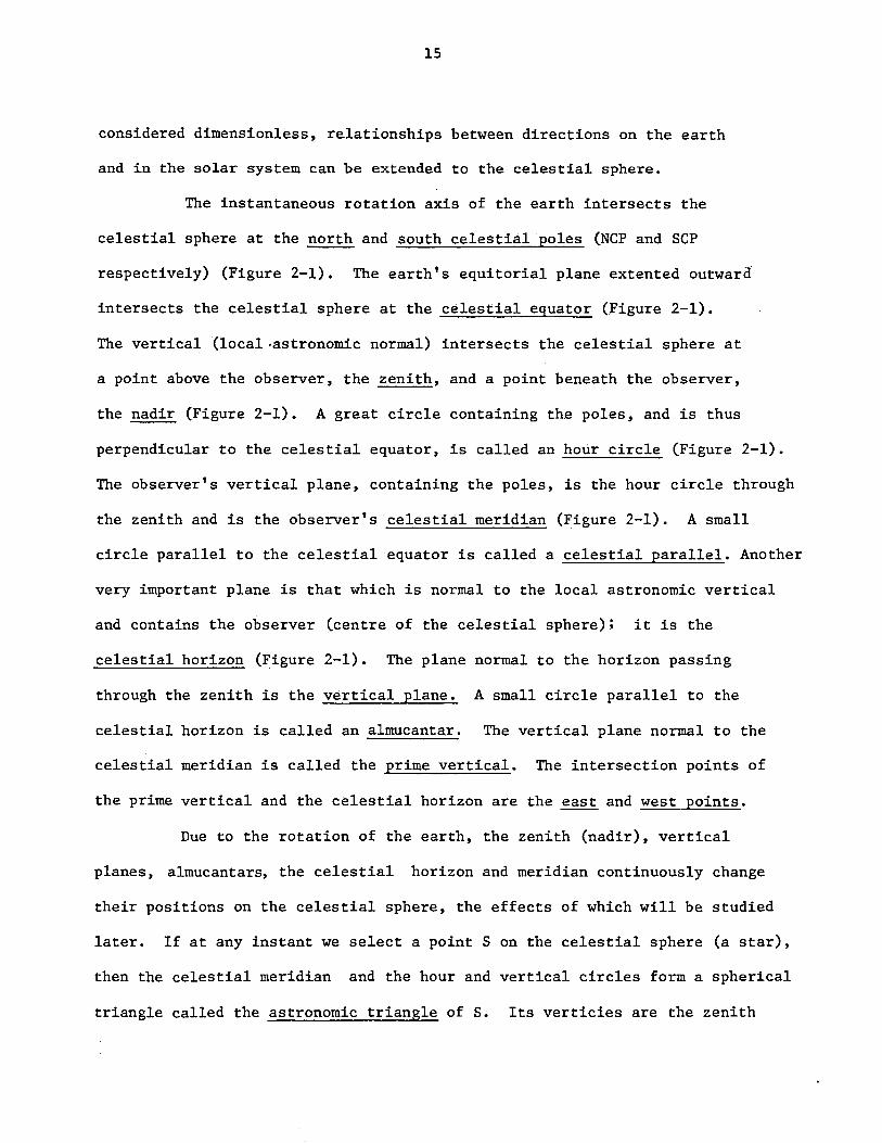
later. If at any instant we select a point S on the celestial sphere (a star),
then the celestial meridian and the hour and vertical circles form a spherical
triangle called the astronomic triangle of S. Its verticies are the zenith
16
NCP
I . I .
. I .
SCP
Figure 2-1
Celestial S h .. p ere
17
I - -I
. Figure 2-2
. c Triangle A~tronoIlU.
18
(Z), the north celestial pole (NCP) and S(Figure 2-2).
There are also some important features on the celestial sphere
related the revolution of the earth about the sun, or in the reversed concept,
the apparent motion of the sun about the earth. The most important of these
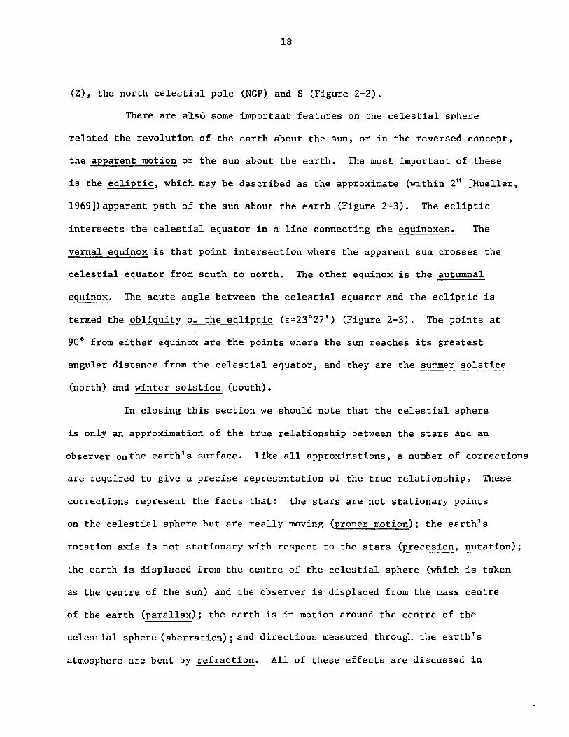
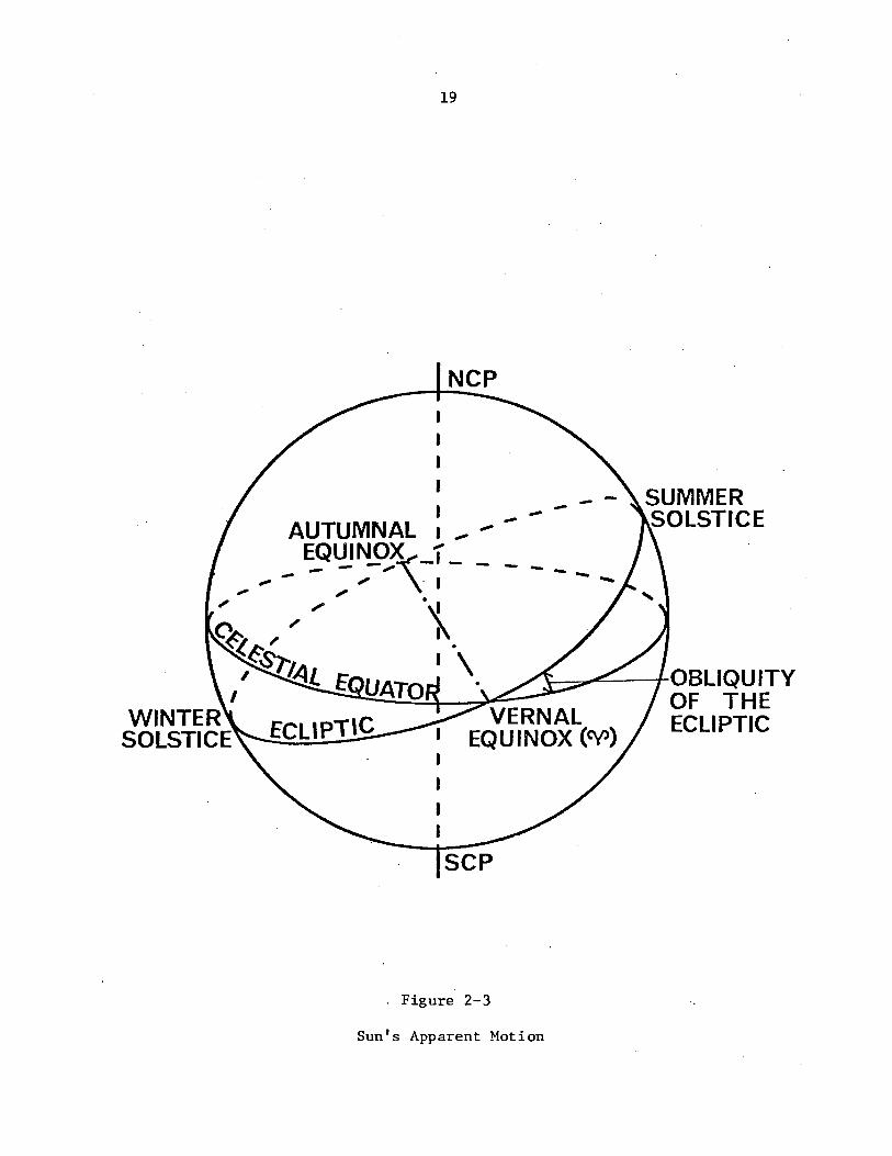
is the ecliptic, which may be described as the approximate (within 2" [Mueller,
1969]) apparent path of the sun about the earth.(Figure 2-3). The ecliptic
intersects the celestial equator in a line connecting theeqtiinoxes. The
vernal equinox is that point intersection where the apparent sun crosses the
celestial equator from south to north. The other equinox is the autumnal
equinox. The acute angle between the celestial equator and the ecliptic is
termed the obliquity of the ecliptic (e:=23°27') (Figure 2-3). The points at
90 0 from either equinox are the points where the sun reaches its greatest
angular distance from the celestial equator, and they are the summer solstice
(north) and winter solstice (south).
In closing this section we should note that the celestial sphere
is only an approximation of the true relationship between the stars and an
observer onthe earth's surface. Like all approximations, a number of corrections
are required to give a precise representation of the true relationship. These
corrections represent the facts that: the stars are not stationary points
on the celestial sphere but are really moving (proper motion); the earth's
rotation axis is not stationary with respect to the stars (precesion, nutation);
the earth is displaced from the centre of the celestial sphere (which is taken
as the centre of the sun) and the observer is displaced from the mass centre
of the earth (parallax); the earth is in motion around the centre of the
celestial sphere (aberration); and directions measured through the earth's
atmosphere are bent by refraction. All of these effects are discussed in
19
I -AUTUMNAL I .". .". -
SUMMER SOLSTICE
_ ~QLEN~X\_I __ ---.". "'" I .... '"
.~
1\ \-----o::~--I-OBL IQ U I TV
---~~~~V~E-R-NAL OF THE I EQU INOX (¥) ECLIPTIC t
I
I I
SCP
. Figure 2-3
Sun's Apparent Motion
20
detail in these notes.
2.2 Celestial Coordinate Systems
Celestial coordinate systems are used to define the positions of
stars on the celestial sphere. Remembering that the distances to the stars
are very great, and in fact can be considered equal thus allowing us to
treat the celestial sphere as a unit sphere, positions are defined by directions
only. One component or curva1inear coordinate is reckoned from a primary
reference plane and is measured perpendicular to it, the other from a
secondary reference p1an~· and is measured in the primary plane.
In these notes, two methods of describing positions are given. The
first is by a set of cur valin ear coordinates, the second by a unit vector
in three dimensional space expressed as a function of the curva1inear
coordinates.
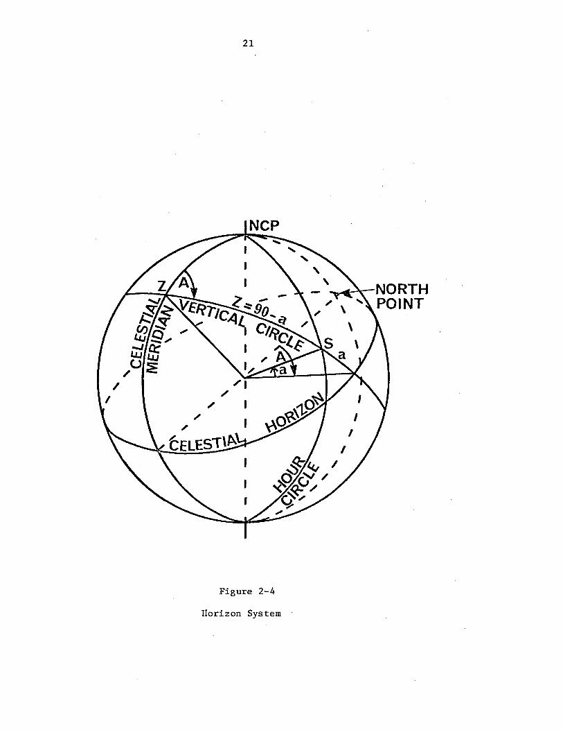
2.2.1 Horizon System
The primary reference plane is the celestial horizon, the secondary
is the observer's celestial meridian (Figure 2-4). This system is used to
describe the position of a celestial body in a system peculiar to a topogra
phically located observer. The direction to the celestial body S is defined
by the a1titude(a) and azimuth (A) (Figure 2-4). The altitude is the angle
between the celestial horizon and the point S measured in the plane of the
vertical circle (0° - 90°). The complimentary angle z =90-a, is called the
zenith distance. The azimuth A is the angle between the observer's celestial
meridian and the vertical circle through S measured in a clockwise direction
(north to east) in the plane of the celestial horizon (0° - 360°).
21
Figure 2-4
Ilorizon System
~~NORTH POINT
22
ZH NCP
Z S
X
~SIN a=Z/1 :o-..~SIN A=Y/COS a
A_ ~ ."
A=X/COS a
Figure 2-5
J!orizon System
I
I
I
x COS a COS A Y . COS a SIN A
Z H SIN a
23
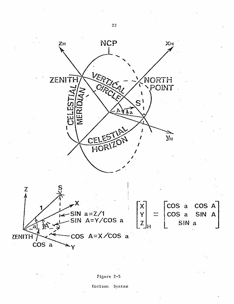
To determine the unit vector of the point S in terms of a and A, we
must first define the origin and the three axes of the coordinate system.
The origin is the he1iocentre (centre of mass of the sun [e.g. Eichorn, 1974]~.
The primary pole (Z) is the observer's zenith (astronomic normal or gravity
vertical). The primary axis (X) is directed towards the north point. The
secondary (Y) axis is chosen so that the system is left-handed (Figure 2-5
illustrates this coordinate system). Note that although the horizon system
is used to describe the position of a celestial body in a system peculiar to
a topographically located observer, the system is heliocentric and not
topocentric.
The unit vector describing the position of S is given by
[cosa COSAJ cosa sinA
sina
T Conversely, a and A, in terms of [X,Y,Z] are (Figure 2-5)
-1 a = sin Z,
-1 Y A = tan (IX).
2.2.2 Hour Angle System
(2-1)
(2-2)
(2-3)
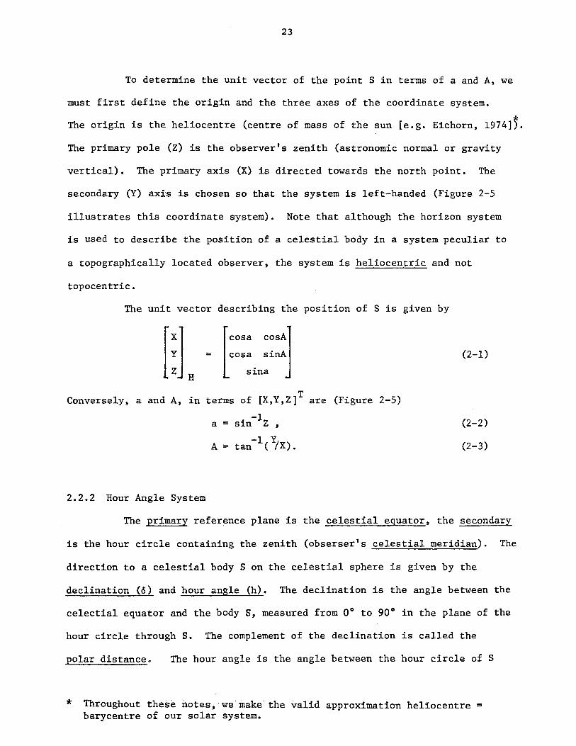
The primary refer~nce plane is the celestial eguator, the secondary
is the hour circle containing the zenith (obserser's celestial meridian). The
direction to a celestial body S on the celestial sphere is given by the
declination (0) and hour angle (h). The declination is the angle between the
ce1ectia1 equator and the body S, measured from 00 to 90 0 in the plane of the
hour circle through S. The complement of the declination is called the
polar distance. The hour angle is the angle between the hour circle of S
* Throughout these notes, wemake'the valid approximation heliocentre = barycentre of our solar system.
24
NCP
Figure 2-6
Hour Angle System
XHA
25
ZHA
x COS 6 COS h Y = COS 6 SIN h Z SIN 6
HA
Figure 2-7
Hour Angle System
26
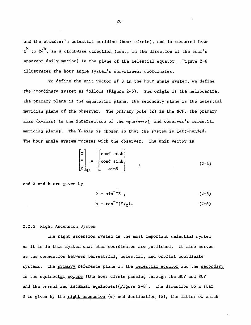
and the observer's celestial meridian (hour circle), and is measured from
h h o to 24 , in a clockwise direction (west, in the direction of the star's
apparent daily motion) in the plane of the celestial equator. Figure 2-6
illustrates the hour angle system's curva1inear coordinates.
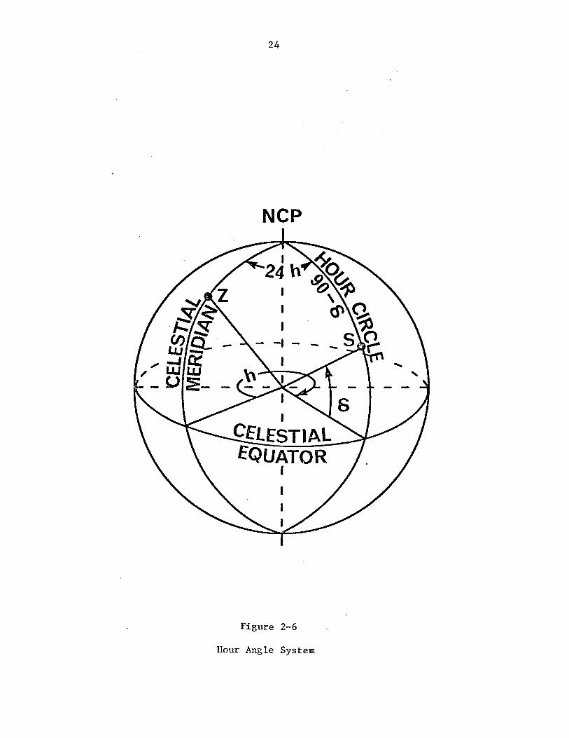
To define the unit vector of S in the hour angle system, we define
the coordinate system as follows (Figure 2-6). The origin is the he1iocentre.
The primary plane is the equatorial plane, the secondary plane is the celestial
meridian plane of the observer. The primary pole (Z) is the NCP, the primary
axis (X-axis) is the intersection of the equatorial and observer's celestial
meridian planes. The Y-axis is chosen so that the system is left-handed.
The hour angle system rotates with the observer. The unit vector is
[XL [coso: COSh] Y • cos& sinh
Z sinS
and ~ and h are given by
o = sin-1Z ,
-1 h = tan (Y/x).
2.2.3 Right Ascension System
, (2-4)
(2-S)
(2-6)
The right ascension system is the most important celestial system
as it is in this system that star coordinates are published. It also serves
as the connection between terrestrial, celestial, and orbital coordinate
systems. The primary reference plane is the celestial equator and the secondary
is the equinocta1 co1ure (the hour circle passing through the NCP and SCP
and the vernal and autumnal equinoxes){Yigure 2-8). The direction to a star
S is given by the right ascension (a) and declination (6), the latter of which
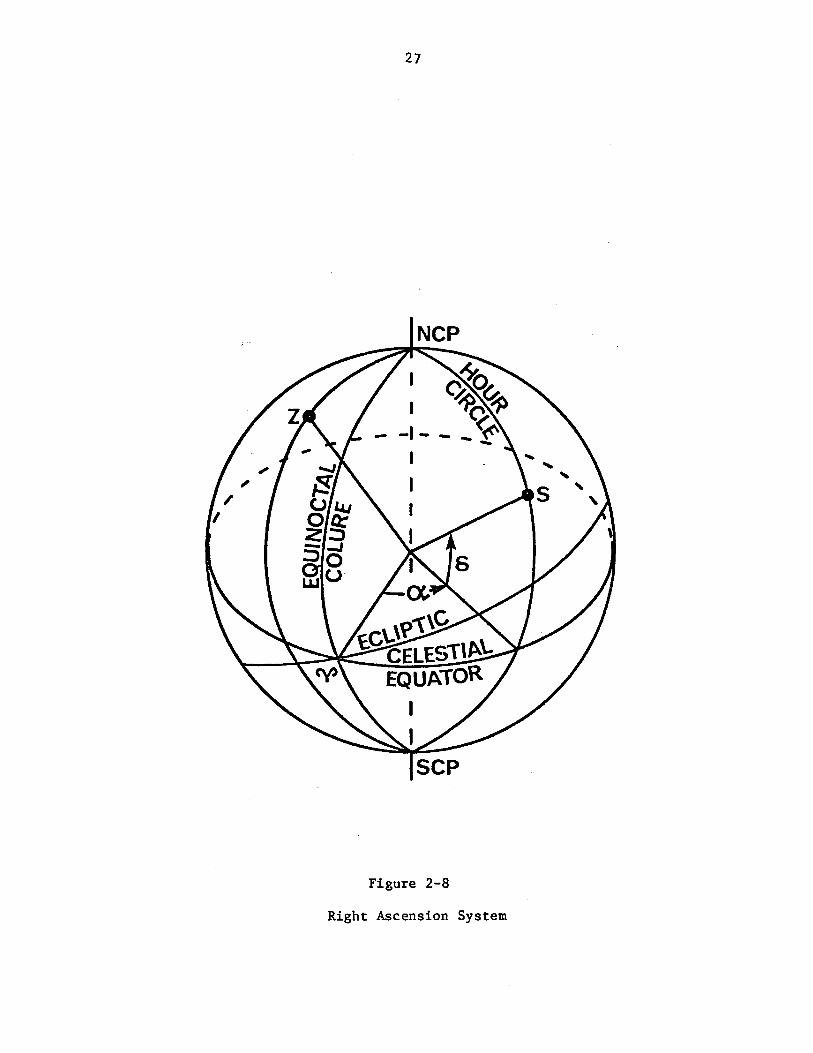
27
NCP
Figure 2-8
Right Ascension System
XRA
28
ZRA
COS 6 COS ~ COS 6 SIN OC
SIN 6
Figure 2-9
Ri~ht Ascension System
YRA

29
has already been defined (RA system). The right ascension is the angle
between the hour circle of S and the equinoctal colure, measured from the
vernal equinox to the east (counter clockwise) in the plane of the celestial
h h equator from 0 to 24 •
The right ascension system coordinate axes are defined as having
a heliocentric origin, with the equatorial plane as the primary plane, the
primary pole (Z) is the NCP, the primary axis (X) is the vernal equinox,
and the Y-axis is chosen to make the system right-handed (Figure 2-9). The
unit vector describing the direction of a body in the right-ascension system
is : ...
X cos' 0 cos<~
Y - cos 15 sino. , (2-7)
Z RA sino
and a and 0 are expressed as -1/<"
a - tan (Y!X) , (2-8)
15 = sin-lz (2-9)
2.2;4 Ecliptic System
The ecliptic system is the celestial coordinate system that is closest
to being inertial, that is, motionless with respect to the stars. However,
due to the effect of the planets on the earth-sun system, the ecliptic plane
is slowly rotating (at '0".5 per year) about a slowly moving axis of rotation.
The primary reference plane is the ecliptic, the secondary reference plane is
the ecliptic meridian of the vernal equinox (contains the north and south
ecliptic poles, the vernal and autumnal equinoxes) (Figure 2-10). The direction
30
SCP
Figure 2-10
Ecliptic System
31
x COS ~ COS A.. Y COS ~ SINA.
Z E SIN ~
Figure 2-11 :.
Ecliptic System
32
to a point S on the celestial sphere .is given by the ecliptic latitude (B)
and ecliptic longitude (A). The ecliptic latitude is the angle, measured
in the ecliptic meridian plane of S, between the ecliptic and the normal OS
(Figure 2~10). The ecliptic longitude is measured eastward in the ecliptic
plane between the ecliptic meridian of the vernal equinox and the ecliptic
meridian of S (Figure 2-10).
The ecliptic system coordinate axes are specified as follows
(Figure 2-11). The origin is heliocentric. The primary plane is the ecliptic
plane and the primary pole (Z) is the NEP (north ecliptic pole). The primary
axis (X) is the normal equinox, and the Y-axis is chosen to make the system
right-handed. The unit vector to S is
x
Y =
Z
while B and A are given by
S =
A =
2.2.5 Summary
cosB COSA
cosS sinA
sinS
-1 sin Z,
-1 tan (y/X)
,
The most important characteristics of the coordinate systems,
(2-10)
(2-11)
(2-12)
expressed in terms of curva1inear coordinates, are given in Table 2-1. The
most important characteristics of the cartesian coordinate systems are shown
in Table 2-2 (Note: ~ and u in Table 2-2 denote the curvilinear coordinates
measured in the primary reference plane and perpendicular to it respectively).
33
Reference Plane Parameters Measured from the
System Primary Secondary Primary Secondary
Horizon Celestial horizon Celestial meridian (half Alti.tude Azimuth containi.ng north pole) -90~!:a !:+900 00<A<3600
(+toward zenith) (+east)
Hour Celestial equa- Hour circle of ob- Declination Hour an~le Angle tor server's zentth (half -90°<15< +90° Oh~h~24h
containing zenith) (+north) 00~h~360° (-+west)
Right Celestial Equinoctical colure Declination Right Ascen Ascension equator (half containing -90°s.15s.+90° \ sion
vernal equinox) (+north) Oh<a.<24h 00~a.~360° (+east)
Ecliptic Ecliptic Ecliptic meridan (Ecliptic) (Ecliptic) equinox (half con- Latitude Longitude taining vernal 90°<6<+90° 0°<:>'<360° equinox) (+n~rth) (+~a~t)
CELESTIAL COORDINATE SYSTEMS [Mueller, 1969]
TABLE 2-1
Orientation of the Positive Axis System X Y Z )J u Left or Right
(Secondary pole) (Primary pole) handed
Horizon North point A .,. 90° Zenith A a left
Intersection of the zenith's hour
90°. 6h Hour angle circle with the h = North celestial h 15 left celestial equator pole on the zenith's side.
Right ascension Vernal equinox a. .,. 90°= 6h North celestial a. 15 right pole
Ecliptic Vernal equinox = 90° North ecliptic :>. 6 right pole
CARTESIAN CELESTIAL COORDINATE SYSTEMS [Mueller, 1969]
TABLE 2-2
34
2.3 Transformations Amongst Celestial Coordinate Systems
Transformations amongst celestial coordinate systems is an important
aspect of geodetic astronomy for it is through the transformation models that
we arrive at the math models for astronomic position and azimuth determination,
Two approaches to coordinate systems transformations are dealt with here:
(i) the traditional approach, using spherical trigonometry, and (ii) a'more
general approach using matrices that is particularly applicable to machine
computations. The relationships that are developped here are between (i)
the horizon and hour angle systems, (ii) the hour angle and right ascension
systems, and (iii) the right ascension and ecliptic systems. With these math
models, anyone system can then be related to any other system (e.g. right
ascension and horizon systemS).
Before developing the transformation models, several more quantities
must be defined. To begin with, the already known quantities relating to the
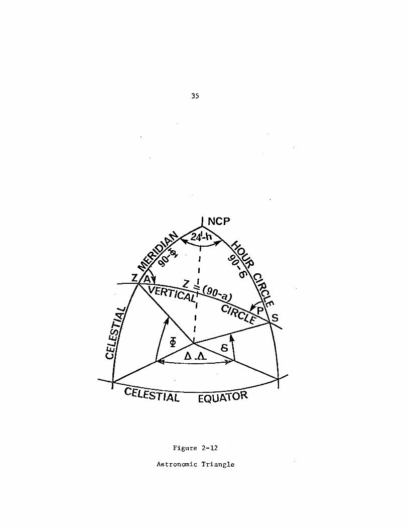
astronomic triangle are (Figure 2-12):
(i) from the horizon system, the astronomic azimuth A and the
altitude a or its compliment the zenith distance z=90-a,
(ii) from the hour angle system, the hour angle h or its compli
ment 24-h,
(iii) from the hour angle or right ascension systems, the declina
tion 0, or its compliment, the polar distance 90-0.
The new quantities required to complete the astronomic triangle are
the astronomic latitude ~ or its compliment 90-~, the difference in astronomic
longitude 6A =As- Az (=24-h), and the parallactic angle p defined as the
angle between the vertical circle and hour circle at S (Figure 2-12).
The last quantity needed is Local Sidereal Time. (Note: this is
35
EQUATOR
Figure 2-12
Astronomic Triangle
36
not a complete definition, but is introduced at this juncture to facilitate
coordinate transformations. A complete discussion of sidereal time is presented
in Chapter 4).
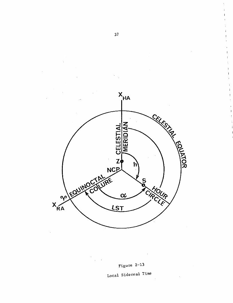
To obtain a definition of Local Sidereal Time, we look at three
meridians: (i) the observer's celestial meridian, (ii) the hour circle
through S, and (iii) the equinoctal colure. Viewing the celestial sphere
from the NCP, we see, on the equatorial plane, the following angles (Figure
2-13): (i) the hour angle (h) between the celestial meridian and the hour
circle (measured clockwise), (ii) the right ascension (a) between the equi-
noctal colure and the hour circle (measured counter clockwise), and (iii)
a new quantity, the Local Sidereal Time (LST) measured clockwise from the
celestial meridian to the equinoctal colure. LST is defined as the hour
angle of the vernal equinox.
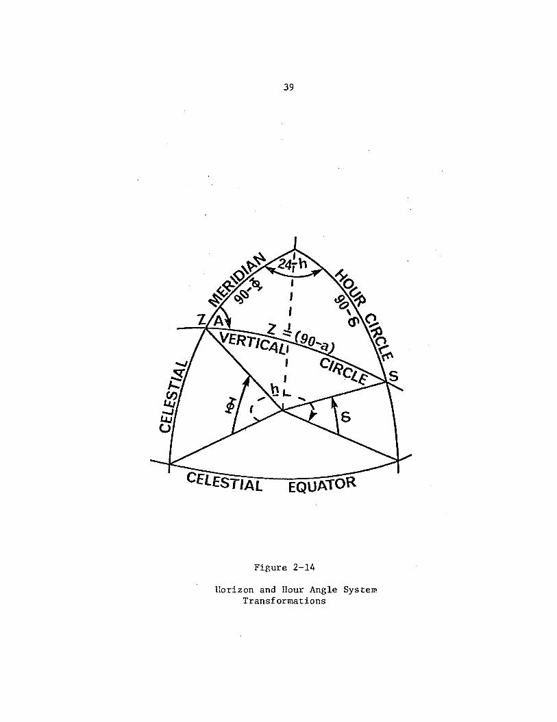
2.3.1 Horizon - Hour Angle
Looking first at the Hour Angle to Horizon system transformation,
using a spherical trigonometric approach, we know that from the hour angle
system we are given h and ~, and we must express these quantities as functions
of the horizon system directions, a (or z) and A. Implicit in this trans-
formation is a knowledge of ~.
From the spherical triangle (Figure 2-14), the law of sines yields
or
and finally
sin(24-h) = sinA ~~77~~
sinz sin(90-~)
-sinh sinz
sinA = ----cos~
sinA sinz = -sinh cos~
, (2-13)
(2-14)
(2-15)
37
....JZ <!
~9 wr:t: ....J w W:E u
Figure 2-13
Local Sidereal Time

38
The five parts formula of spherical trigonometry gives
cosA sinz = cos(90-~)sin(90-~)-cos(90-~)sin(90-~)cos(24-h), or
cosA sinz = sin6 cos~ - sin~ cos6 cosh
Now, dividing (2-15) by (2-17) yields
sini\. sinz cosA sinz = -sinh cos~
sin6 cos~ -sin~ coso cosh
(2-16)
(2-17)
(2-18)
which, after cancelling and collecting terms and dividing the numerator and
denominator of the right-hand-side by coso yields
tanA = -sinh tan~ cos~ -sin~ cosh
, (2-19)
or
tanA = sinh (2-20) sin~ cosh - tano cos~
Finally, the cosine law gives
cosz = cos(90-~)cos(90-9) + sin(90-~)sin(90-9)COs(24-h), (2-21)
or
cost = sin~ sino + cos~ coso cosh (2-22)
Thus, through equations (2-20) and (2-22), we have the desired
results - the quantities a (z) and A expressed as functions of 0 and h and a
known latitude ~.
The transformation Horizon to Hour Angle system (given a (=90-z),
A, ~, compute h, 0) is done in a similar way using spherical trigonometry.
The sine law yields
coso sinh = -sinz sinA , (2-23)
and five parts gives,
coso cosh = cosz cos~ -sinz cosA sin~ (2-24)
39
EQUATOR
Figure 2-14
llorizonand Hour Angle System Transformations
40
After dividing (2-23) by (2-24), the result is
tanh _ __~ __ s7i=nA~ ________ ~ cosA sin~ -cotz cos~ (2-25)
Finally,the cosine law yields
sineS = cosz sin~ + sinz cosA cos~ (2-26)
Equations (2-25) and (2-26) are the desired results - hand eS expressed
solely as functions of a(=90-z),A, and ~.
Another approach to the solution of these transformations
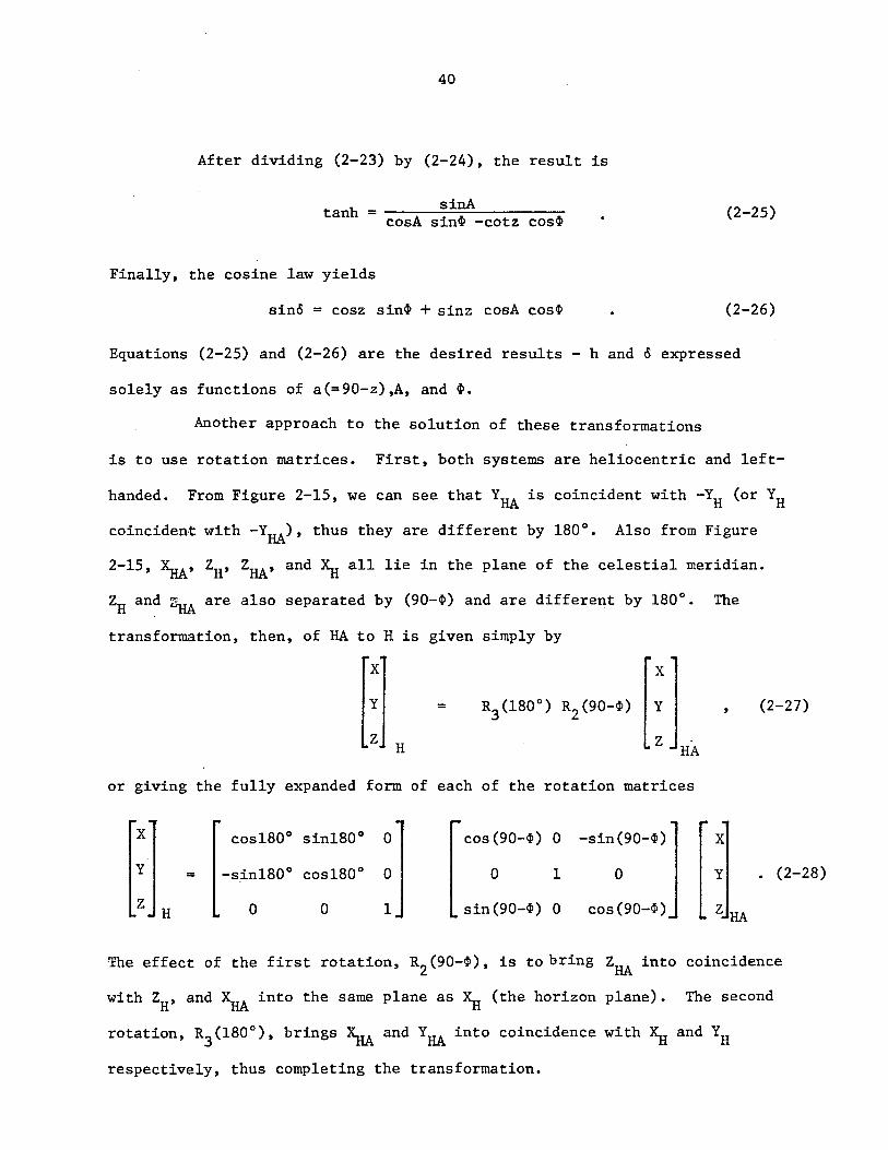
is to use rotation matrices. First, both systems are heliocentric and left-
handed. From Figure 2-15, we can see that YHA is coincident with -YH (or YH
coincident with -YHA), thus they are different by 180°. Also from Figure
2-15, ~, ZH' ZHA' and ~ all lie in the plane of the celestial meridian.
ZH an~ ~ are also separated by (90-~) and are different by 180°.
transformation, then, of HA to H is given simply by
x x
The
y = (2-27)
Z H Z HA
or giving the fully expanded form of each of the rotation matrices
X cos180° sin1800 0 cos(90-~) 0 -sin(90-~) X
Y = -s.in1800 cos180° 0 0 1 0 Y . (2-28)
Z H 0 0 1 sin(90-~) 0 cos (90-11» ZHA
The effect of the first rotation, R2 (90-11», is to bring ZHA into coincidence
with ZH' and ~ into the same plane as ~ (the horizon plane). The second
rotation, R3 (1800), brings ~ and YHA into coincidence with ~ and YH
respectively, thus completing the transformation.
41
NCP
2-15 Figure
Angle Systems and Hour Horizon .
EAST POINT
42
The reverse transformation - Horizon to Hour Angle - is simply
the inverse* of (2-27), namely
= (2-29)
H
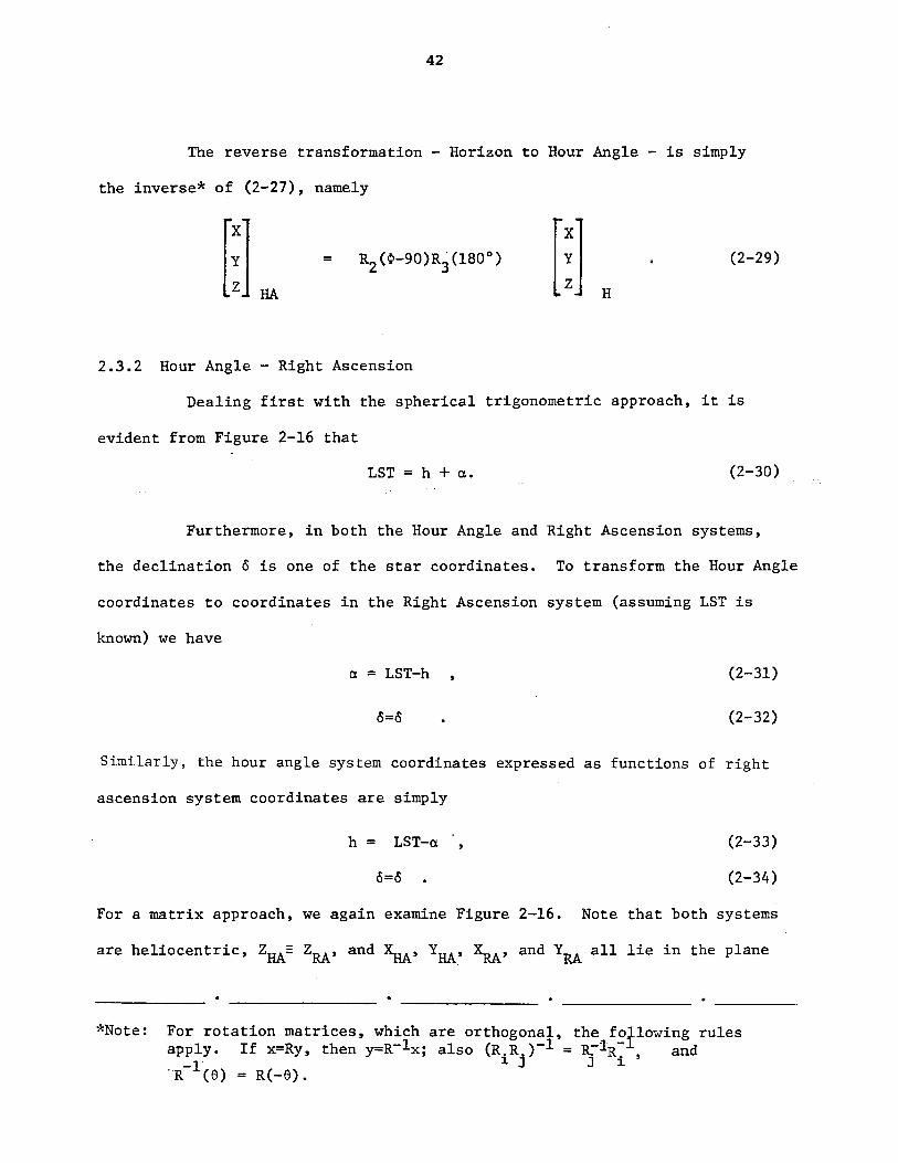
2.3.2 Hour Angle - Right Ascension
Dealing first with the spherical trigonometric approach, it is
evident from Figure 2-16 that
LST = h + a. (2-30)
Furthermore, in both the Hour Angle and Right Ascension systems,
the declination 0 is one of the star coordinates. To transform the Hour Angle
coordinates to coordinates in the Right Ascension system (assuming LST is
known) we have
a = LST-h (2-31)
0=0 (2-32)
Similarly, the hour angle system coordinates expressed as functions of right
aS,cension system coordinates are simply
h = LST-a (2-33)
0=0 (2-34)
For a matrix approach, we again examine Figure 2-16. Note that both systems
are heliocentric, ZHA= ZRA' and ~, YHA,' ~, and YRA all lie in the plane
*Note: For rotation matrices, which are orthogonal, the .. f~t1owing rules apply. If x=Ry, then y=R-1x ; also (Ri Rj )-l = ~lRi' and 'R-1 '(S) == R(-S).
43
Figure 2-16
Hour Ang1e·- Right Ascension Systems
44
of the celestial equator. The differences are that the HA system is left-
handed, the RA system right-handed, and XHA and ~ are separated by the
LST. The Right Ascension system, in terms of the hour angle system, is
given by
or, with R3(-LST) and the ,reflection matrix P2 expanded,
[x] [ cos(-LST) sin(-LST)
~ ~ -Sin(~LST) COS(~LST) ~] [~ o
-1
o
(2-35)
(2-36)
The reflection matrix, P2, changes the handedness of the hour angle system
(from left to right), and the rotation R3 (-LST) brings XHA and YHA into coin
cidence with ~ and YRA respectively.
The inverse trans~ormation is simply
(2-37)
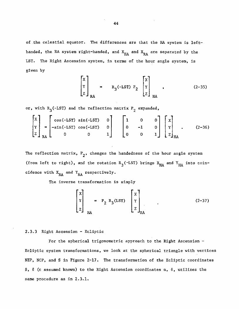
2.3.3 Right Ascension - Ecliptic
For the spherical trigonometric approach to the Right Ascension -
Ecliptic system transformations, we look at the spherical triangle with vertices
NEP, NCP, and S in .Figure 2~17. The transformation of the Ecliptic coordinates
B, 6 (€ assumed known) to the Right Ascension coordinates a, 0, utilizes the
same procedure as in 2.3.1.
o -h: -..I ~
45
Z RA
CELESTIAL
Figure 2-17
c ystems Right Ascension-Ec1ipti S'
SUMMER SOLSTICE
YE
· 46
The sine rule of spherical trigonometry yields
coso cosa == cos~ cosA
and the five parts rule
coso sina = cos~ sinA COSE - sinS sinE
Dividing (2-39) by (2-38) yields the desired result
tana =
From the cosine rule
sinA COSE - tanS SinE cosA
sino = cos~ sinA sinE + sinS COSE ,
which completes the transformation of the Ecliptic system to the Right
Ascension system.
(2-38)
(2-39)
(2-40)
(2-41)
Using the same rules of spherical trigonometry (sine, five-parts,
cosine), the inverse transformation (Right Ascension to Ecliptic) is given
by
cosS co.sA == coso cosa ,
cosS sinA = coso sina COSE + sino sinE ,
which, after dividing (2-43) by (2-42) yields
and
tanA == sina COSE + tano sinE
cosa
sinS = -coso sina sinE + sino COSE •
(2-42)
(2-43)
(2-44)
(2-45)
From Figure 2-17, it is evident that the difference between the
E and RA cartesian systems is simply the obliquity of the ecliptic, E, which
separates the ZE and ZRA' and YE and YRA axes, the pairs of which lie in the
same planes.
47
The transformations then are given by
[:lll = R (-e:) 1 [~L (2-46)
and
[:] == Rl(e:) [~] II (2-47)
E
2.3.4 Summary
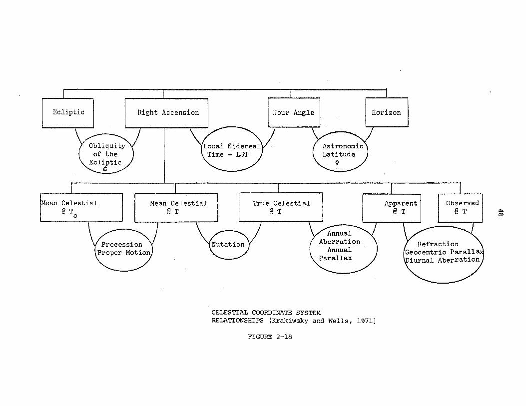
Figure 2-18 and Table 2-3 summarize the transformations amongst
celestial coordinate systems. Note that in Figure 2-18, the quantities that
we must know to effect the various transformations are highlighted. In addition,
Figure 2-18 highlights the expansion of the Right Ascension system to account
for the motions of the coordinate systems in time and space as mentioned in
the introduction to this chapter. These effects are covered in detail in
Chapter 3.
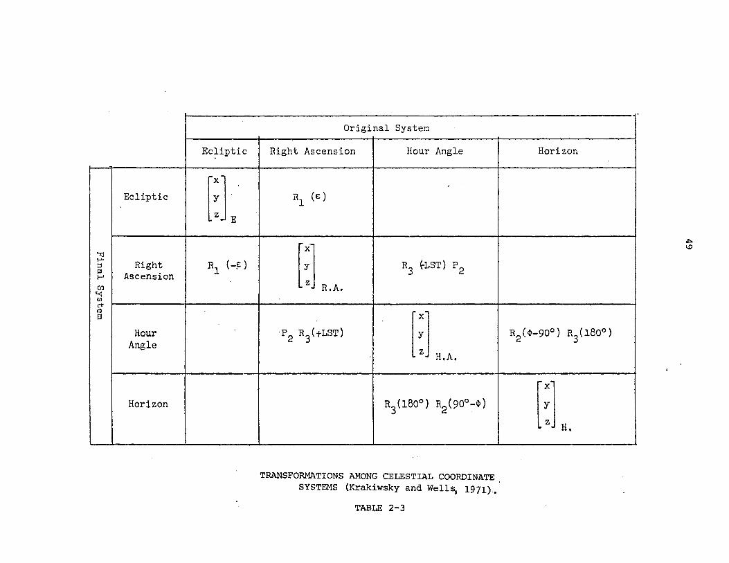
Table 2-3 highlights the matrix approach to the transformations
amongst celestial coordinate systems.
2.4 Special Star Positions
Certain positions of stars on the celestial sphere are given "special"
names. As shall be seen later, some of the math models for astronomic position
and azimuth determination are based on some of the special positions that
stars attain.
ECliptic
If'1ea:~elestial @ T
o
Right Ascension
Mean Celestial @ T
Hour Angle
True Celestial @ T
I-~--
I
I H • I orlzon
Apparent @ T
CELESTIAL COORDINATE SYSTEM RELATIONSHIPS [Krakiwsky and Wells, 1971J
FIGURE 2-18
.::. 0:>
Ecliptic
Ecliptic rXl . I .
l:J E
'"%j ...,-
Right iiI (-~) ::s 10 Ascension I-'
Cf) «: (Jl
c+ (j)
a
Hour Angle
Horizon
Original System
Right Ascension Hour Angle
,
RI (E:)
fXi
l:j R.A.
R3 tLST) P 2
P 2 R3(tLST) [:J H.A.
R3(1800) R2(900-~)
TRANSFO~~TIONS AMONG CELESTIAL COORDINATE SYSTEMS (Krakiwsky and Wells, 1971) .•
TABLE 2-3
Horizon
R2(~-900) R3(1800)
[:L,
,
,/:>0 1.0
50
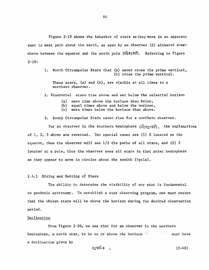
Figure 2-19 shows the behavior of stars as they move in an apparent
east to west path about the earth, as seen by an observer (Z) situated some
where between the equator and the north pole (0~~S9d). Referring to Figure
2-19:
1. North Circumpolar Stars that (a) never cross the prime vertical, (b) cross the prime vertical.
These stars, (a) and (b), are visible at all times to a northern observer.
2. Equatorial stars rise above and set below the celestial horizon
(a) more time above the horizon than below, (b) equal times above and below the horizon, (c) more times below the horizon than above.
3. South Circumpolar Stars never rise for a northern observer.
For an observer in the southern hemisphere (O~~~;:99i, the explanations
of 1, 2, 3 above are reversed. Two special cases are (1) Z located on the
equator, thus the observer will see 1/2 the paths of all stars, and (2) Z
located at a pole, thus the observer sees all stars in that polar hemisphere
as they appear to move in circles about the zenith (=po1e).
2.4.1 Rising and Setting of Stars
The ability to determine the visibility of any star is fundamental
to geodetic astronomy. To establish a star observing program, one must ensure
that the chosen stars will be above the horizon during the desired observation
period.
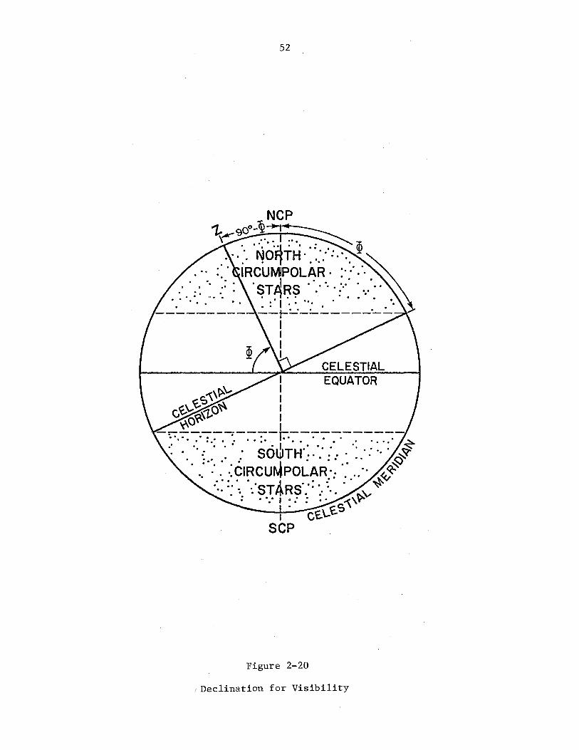
Declination
From Figure 2-20, we see that for an observer in the northern
hemisphere, a north star, to be on or above the horizon - must have
a declination given by o
c5~90-~ , (2-48)
51
Figure 2-19
Circumpolar and Equatorial Stars
52
I I I I I I
CELESTIAL EQUATOR
-----------r-----------"'ull II> .. 0 .. .. I._ III.. It ..
.. .. .. .. III'" .. .. .. '" .111 .. .. .... 'It .. .... ~
.'" 011 "".. '" .." .. .. I .. .. ".." ... It ...... ~ '. SO':ITH .. ..' .' ..... "f
III .. III e.. \J,I .. 8.... .. .. ~'
.. :'::~ ::~I~CU~POL~R.:: ': .. :. ~~ 'e. e.. e 'ST ARS' ..... ~
It.... "" ........ • "'-v : .. " .. " I .: : .. " ~\r
I· C'E.~'E.S SCP
Figure 2-20
! Declination for Visibility
53 .
and a south star that will rise at some time, must have a declination
(2-49)
Thus, the condition for rising and setting of a star is
o 0 90-IP>e>4>-90. (2-50)
For example, at Fredericton, where IP= 46°N, the declination of a star must
always satisfy the condition (2-50), namely
in order that the star will be visible at some time; that is, the star will
rise and set. If 15>44°, the star will never set (it will always be a visible
circumpolar star), and if 15<-44°, the star will never rise (a south circumpolar
star).
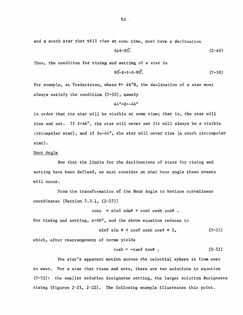
Hour Angle
Now that the limits for the declinations of stars for rising and
setting have been defined, we must consider at what hour angle these events
will occur.
From the transformation of the Hour Angle to Horizon curvalinear
coordinates (Section 2.3.1, (2-22»
cosz = sine sin4> + cose cosh cos4> •
For rising and setting,· z=90o, and the above equation reduces to
sine sin IP + cose cosh coslP = 0, (2-51)
which, after rearrangement of terms yields
cosh = -tane tan4> • (2-52)
The star's apparent motion across the celestial sphere is from east
to west. For a star that rises and sets, there are two solutions to equation
(2-52): the smaller solution designates setting, the larger solution designates
rising (Figures 2-21, 2-22). The following example illustrates this point.
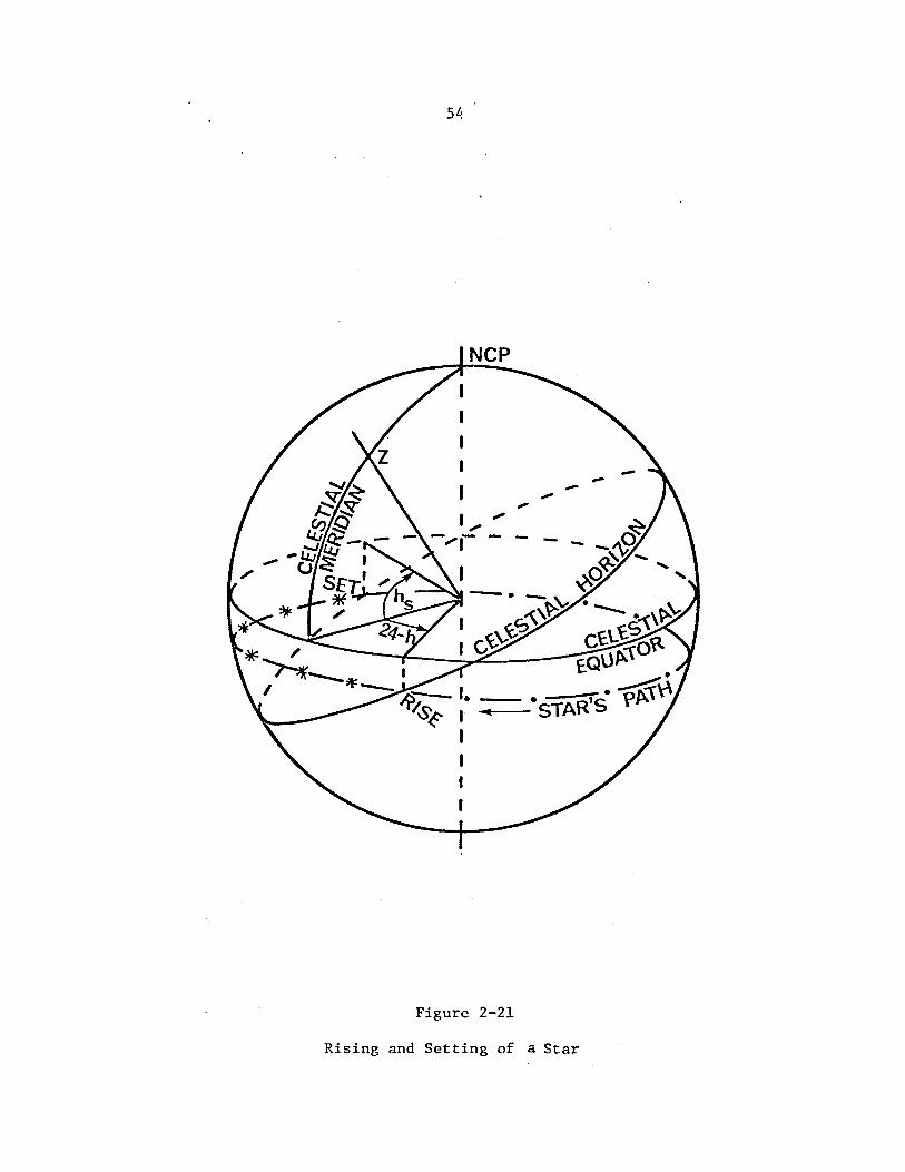
Rising
Figure 2-21
and Settl.n f a Star . g 0
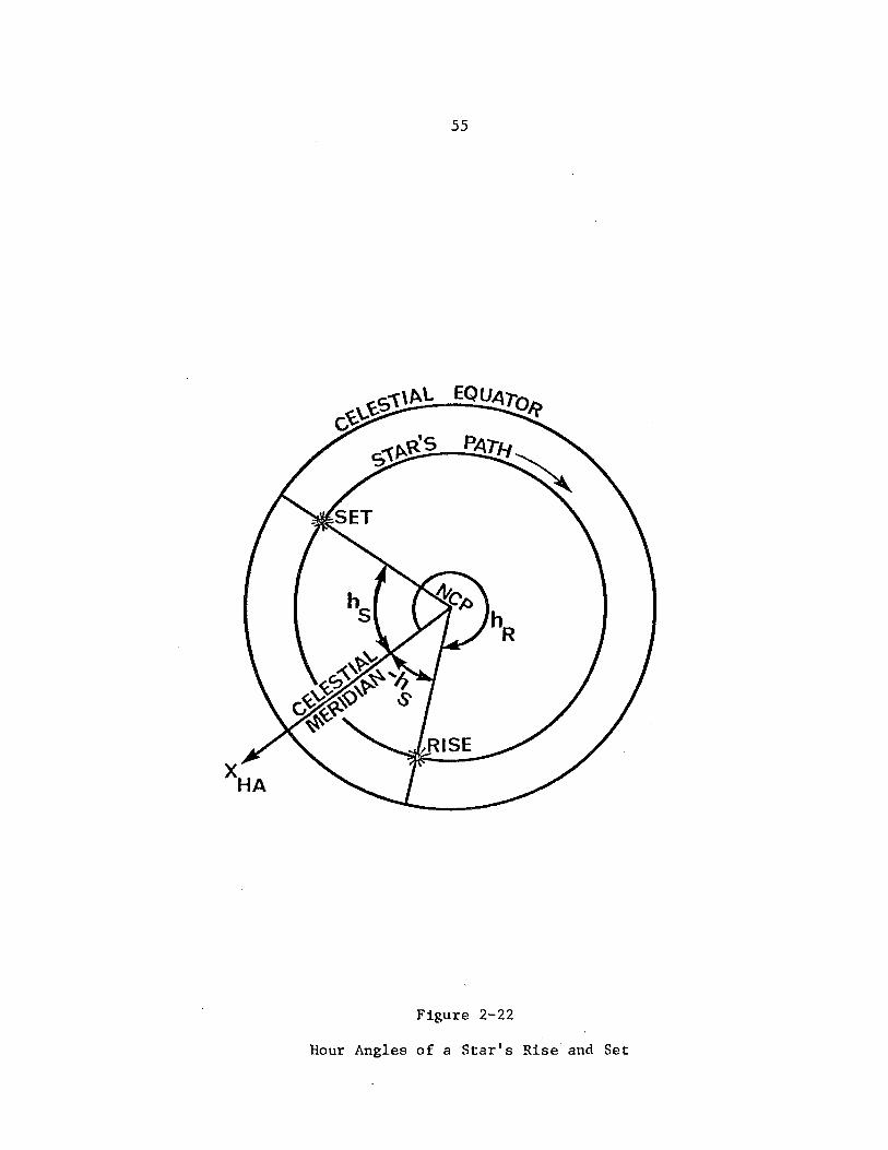
55
Figure 2-22
Hour Angles of a Star's Rise and Set
56
At ~=46°, we wish to investigate the possible use of two stars for
an observation program. Their declinations are 01=35°, 02=50°. From equation
(2-50),
44°<°2< - 44°.
The first star, since it satisfies (2-50), will rise and set. The second star,
since 02> 44°, never sets - it is a north circumpolar star to our observer.
Continuing with the first star, equation (2-52) yields
coshl = -tan35° tan46°
or
which is the hour angle for setting. The hour angle for rising is
hr = (24h_£s) = l4h 54m 05~78. 1 1
Azimuth
At what azimuth will a star rise or set? From the sine law in the
Hour Anglet:o Horizon system trans-fomtion. (equation (2-15»
sinz sinA = -coso sinh.
With z=900 for rising and setting, then
sinA = -coso sinh. (2-53)
There are, of course, two solutions (Figures 2-23 and 2-24): one
using hr and one using hS• Using the previous example for star 1 (01=35°,
~=46°, h~ = 9h 05m 54~22, h~ = 14h 54m 05~78), one gets
Similarly
SinA~ = -cos 35° sin 223~524l,
Ar = 34° 20' 27~64. 1
AS = 325° 39' 32~36. 1
57
I I NORTH \ I POINt
,
Figure 2-23
Ri . s~ng and Setting of a Star
58
:Fisure 2-24
Azimuths of a Star's Rise and Set
59
The following set of rules apply for the hour angles and azimuths of rising
and setting stars [Mueller, 1969]:
Northern Stars ·t<5>OO) Rise 12h<h<18h 00<A<900
Set 6h<h<12h 2700<A<360°
Equatorial Stars (<5=0°) Rise h=18h A=900
Set h= 6h A=270°
Southern Stars Rise 18h<h<24h 900<A<l800
Set Oh<h< 6h 1800<A<2700
2.4.2 Culmination (Transit)
When a star's hour circle is coincident with the observer's celestial
meridian, it is said to culminate or transit. Upper culmination (UC) is defined
as being on the zenith side of the hour circle, and can occur north or south
of the zenith (Figure 2-25a and 2.-25b). When UC occurs north of Z, the zenith
distance is given as (Figure 25a)
z = <5-~ • (2-54)
The zenith distance of UC south of Z is
z = 41-<5 • (2-55)
Lower Culmination (LC) (Figure 2-25c) is on the nadir side of the hour circle,
and for a northern observer, always occurs north of the zenith. The zenith
distance at LC is
z = 180- (<5+41 ) •
Recalling the examples given in 2.4.1 (~=46o,<51 =35°, <5 2=50°),
then for the first star
which is south of the zenith, and
(2-56)
.' I ' ,
60
, , ,
Figure 2-25
(A) UPPER CULMINATION
(8) UPPER CULMINATION
(C) LOWER CULMINATION
Culmination (Transit)
61
LC zl = 180 -(ol+~) = 99°
which means that the star will not be visible (z>900).
For the second star, one obtains
UC z2 = 02-~ = 4° ,
both of which will be north of the zenith. The hour angle at culmination
is h = Oh for all upper culminations, and h = l2h for all lower culminations.
The azimuths at culmination are as follows: A = 0° for all Upper Culminations
north of Z and all Lower Culminations; A = 180° for all Upper Culminations
south of the zenith.
Recalling the Hour Angle - Right Ascension coordinate transformations,
we had (equation (2-30)
LST = h+a •
Since h = Oh for Upper Culminations and h = l2h for Lower Culminations,
2.4.3. Prime Vertical Crossing
LSTUC = LC
LST =
(l ,
For a star to reach the prime vertical (Figure 2-26)
(2-57)
(2-58)
(2-59)
To compute the zenith distance of a prime vertical crossing, recall
from the Horizon to Hour Angle transformation (via) the cosine rule, equation (2-26)
that
sino = coszsin~ + sinz cosA cos~
For a prime vertical crossing in the east, A=90° ~ltitude increasing), and
for a prime vertical crossing in the west, A=270° (altitUde decreasing),
PRIME VERTICAL· CROSSING (WEST)
62
Figure 2--26
Prime Vertical Crossine

63
we get
COSE 'sino =--sin\l> = sin~ cosecl%> (2-60)
The hour angle of a prime vertical crossing is computed as follows. From the
cosine rule of the Hour Angle to Horizon transformation (equation (2-22»
cosz = sino sinl%> + coso cosh cosl%> •
Substituting (2-60) in the above for cosine z yields
or
sino sinl%> = sino sinl%> + coso cosh cosl%> •
2 sino = sino sin~ + coso cosh cos~ sinl%> •
Now, (2-61) reduces to
or
and finally
sino cosh = --~~~~--~~ coso cqsl%> sinl%>
cosh =
cosh = tano cotl%>
2 sino sin I%>
coso cosl%> sinl%>
2 tano ( cos I%> )
cosl%> sinl%>
(2-61)
(2-62)
As with the determination of the rising and setting of a star, there are two
values for h - prime vertical eastern crossing (18h<h<24h) and prime vertical
western crossing (Oh<h<6h). Continuing with the previous examples (01 = 35°,
O2 = 50°), it is immediately evident that the second star will not cross the
The first star will cross the prime vertical
(0<01< 46°), with azimuths A=900 (eastern) and A=270° (western). The zenith
distance for both crossings will be (equation 2-60)
sin 35° cosz1 = sin 46°
z = 37° 07' 14~8. 1
The hour angles of western and eastern crossings are respectively (equation 2-62)
and
2.4.4. Elongation
64
W cosh2 = tanl5 cot~
= tan 35° cot 46° ,
~ = 47~45397 = 3h09m48~9 I
When the parallactic angle (p) is 90°, that is, the hour circle and
vertical circle are normal to each other, the star is said to be at elongation
(Figure 1-27). Elongation can occur on both sides of the observer's celestial
meridian, but only with stars that do not cross the prime vertical. Thus,
the condition for elongation is that
15>!%> • (2-63)
From the astronomic triangle (Figure 2-27), the sine law yields
or
sinA sinp sin(90-15)= ~s~in~(9~0~-~!%>~) ,
sinA = sinp cosl5 cos!%>
Since at elongation, p=900, (2-64) becomes
sinA = cosl5 sec!%> •
(2-64)
(2-65)
For eastern elongation, it is obvious that 00<A<900, and for western
elongation 2700<A<360° •.
To solve for the zenith distance and hour angle at elongation, one
proceeds as follows. Using the cosine law with the astronomic triangle
(Figure 1-27), one gets
cos(90-!%» = cos(90-o)cosz+sinz sin(90-o)cosp , (2-66)
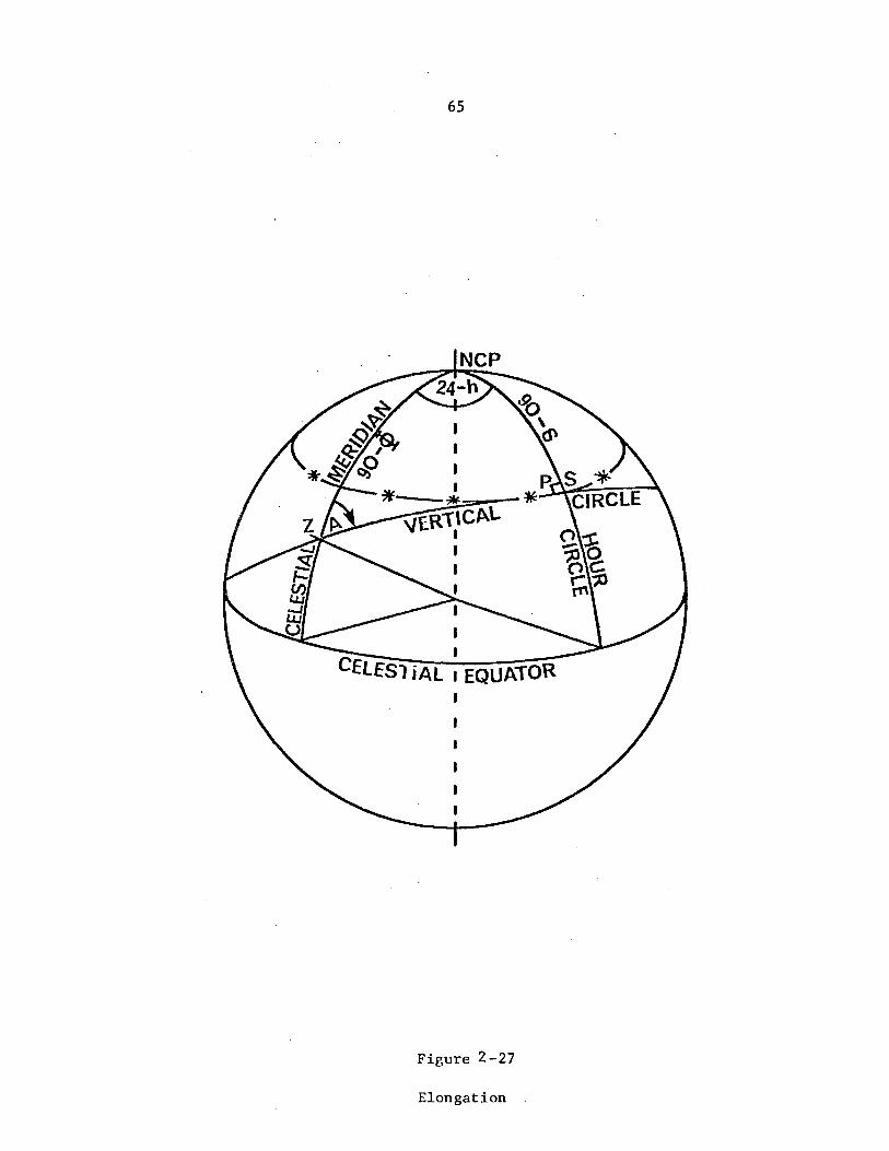
65
CELESl iAl I EQUATOR
Figure 2-27
Elongation
66
and when p=90°, cosp=O, then
cosz = sin~cosec~ • (2-67)
Now, substituting the above expression for cosz (2-67) in the Hour
Angle to Horizon coordinate transformation expression ,(2-22), namely
cosz = sin~ sin~ + cos~ cosh cos~
yields
sin~
sin& = sin~ sin~ + cos~ cosh cos~
which, on rearranging terms gives 2
cosh = sin~ - sin,~ sin~
cosl5 sinl5 cos~
Further manipulation of (2-68) leads to
l-sin26 ~ cos20 cosh = tan~ ( ) = tan~ ( ) cos6sin& cos& sin& ,
and finally
cosh = tan~ cot& •
,
,
:(2-68)
(2-69)
Note that as with the azimuth at elongation, one will have an eastern and
western value for the hour angle.
Continuing with the previous examples ~ ~1=35°, 02=50°, and ~=46° -
we see that for the first star, &l<~' thus it does not elongate. For the second
star~ &2>~ (500~46°), thus eastern and western elongations will occur. The
azimuths, zenith, distance, and hour angles for the second star are as follows:
SinA~ = cos6 sec~ == cos 50° sec 46° ,
AE == 67° 43' 04~7 , 2
AW = 360° _AW == 292° 16' 55~3'; 2 2
cosZ == sin~ cosec~ = sin 46° cosec 50°. ,
z == 20° 06' 37~3 ; 2
tan~ coto == tan 46° cot 50°
3 • TIME SYSTEMS
In the beginning of Chapter 2, it was pointed out that the
position of a star on the celestial sphere, in any of the four coordinates
systems, is valid for only one instant of time T. Due to many factors
Ce.g. earth's motions, motions of stars), the celestial coordinates are
subject to change with time. To fully understand these variations, one
must be familiar with the time systems that are used.
To describe time systems, there are three basic definitions that
have to be stated. An epoch is a particular instant of time used to define
the instant of occurance of some phenomenon or observation. A time
interval is the time elapsed between two epochs, and is measured in some time
scale. For civil time (the time used for everyday purposes) the units of
a time scale (e.g. seconds) are considered fixed in length. With astronomic
time systems, the units vary in length for each system. The adopted unit
of time should be related to some repetitive physical phenomenon so that it
can be easily and reliably established. The phenomenon should be free, or
capable of being freed, from short period irregularities to permit
interpolation and extrapolation by man-made time-keeping devices.
There are three basic time systems:
<.1) Sidereal and Universal Time, based on the diurnal rotation of
the earth and determined by star observations,
(2) Atomic Time, based on the period of electro magnetic oscillations
produced by the quantum transition of the atom of Caesium 133,
(3) Ephemeris Time, defined via the orbital motion of the earth about
the sun.
Ephemeris time is used mainly in the field of celestial mechanics
and is of little interest in geodetic astronomy. Sidereal and Universal
67
68
times are the most useful for geodetic purposes. They are related to each
other via ri90rouS formulae, thus the use of one or the other is purely
a matter of convenience. All broadcast time si9na1s 'are derived from Atomi
time, thus the relationship between Atomic time and Sidereal or universal
time is important for geodetic astronomy.
3.1 Sidereal Time
The fundamental unit of the sidereal time interval is the mean
sidereal day. This is defined as the interval between two successive upper
transits of the mean vernal equinox (the position of T for which uniform
precessional motion is accounted for and short period non-uniform nutation
is removed) over some meridian (the effects of polar motion on the
meridian are removed). The mean sidereal day is reckoned from Oh at upper
transit, which is known as sidereal noon. The units are 1h = 60m , s s
1m = 60s • Apparent (true) sidereal time (the position of T is affected s s
by both precession and nutation), because of its variable (non-uniform)
rate, is not used as a measure of time interval. Since the mean equinox
is affected only be precession (nutation effects are removed), the mean
sidereal day is 0~0084 shorter than the actual rotation period of the s
earth.
From the above definition of the fundamental unit of the
sidereal time interval, we see that sidereal time is directly related to
the rotation of the earth - equal an9les of an9Ular motion correspond to
equal intervals of sidereal time. The sidereal epoch is numerically
measured by the hour angle of the vernal equinox. The hour angle of the
true vernal equinox (position of T affected by precession and nutation)
is termed Local Apparent Sidereal Time (LAST). When the hour angle
69
measured is that at the Greenwich mean astronomic meridian (GHA), it is
called Greenwich Apparent Sidereal Time (GAST). Note that the use of the
Greenwich meridian as.a reference meridian for time systems is one of
convenience and uniformity. This convenience and uniformity gives us
the direct relationships between time and longitude, as well as the
simplicity of publishing star coordinates that are independent of, but
directly related to, the longitude of an observer. The local hour angle
of the mean vernal equinox is called Local Mean Sidereal Time (LMST), and
the Greenwich hour a,ng1e of the mean vernal equinox is the Greenwich Mean
Sidereal Time (GMST). The difference between LAST and LMST, or equivalently,
GAST and GMST, is called the Equation of the Equinoxes (Eq. E), namely
Eq.E = LAST ~ LMST = GAST - GMST. (3-1)
LAST, LMST, GAST, GMST, and Eq.E are all shown in Figure 3-1.
The equation of the equinoxes is due to nutation and varies
periodically with a maximum amplitude near 1s (Figure 3-2). It is f,;
tabulated for Oh U.T. (see 3.2) for each day of the year, in the Astromica1
Almanac (AA), formerly called the American Ephemeris and Nautical Almanac (AENA)
[U.S. Naval Observatory, 1980].
To obtain the relationships between Local and Greenwich times,
we require the longitude (II.) of a place. Then, from Figure 3-3, it can
be seen that
LMST = GMST + A ( 3-2)
LAST = GAST + A , (3-3)
in which A is the "reduced" astronomic longitude of the local meridian
(corrections for polar motion have been made) measured east from the
Greenwich meridian.
70
Figure 3-1
Sidereal Time Epochs
s -0.65
s -0.70
s -0.75
s -0.80
s -0.85
s -0.90
s -0.95
71
~-"+---+---;---~--~--~---r---r-"-+-"-+--~--~--~
JAN. MAR. MAY JULY SEPT.
Figure 3-2
Equation of Equinoxes (OhUT , 1966) [Mueller. 1969]
NOV. JAN.
¥ TRUE
72
NCP
Figure 3-3
Sidereal Time and Lorigitude
73
For the purpose of tabulating certain quantities with arguements
of sidereal time, the concept of Greenwich Sidereal pate (G.S.D.) and
Greenwich Sidereal Day Number are used. The G.S.D. is the number of mean
sidereal days that have elapsed on the Greenwich mean astronomic meridian
since the beginning of the sidereal day that was in progress at Greenwich
noon on Jan. 1, 4713 B.C. The integral part of the G.S.D. is the Greenwich
Sidereal Day Number, and the fractional part is the GMST expressed as a
fraction of a day. Figure 3-4, which is part of one of the tables from
AA shows the G.S.D.
74
UNIVERSAL AND SIDEREAL TIMES, 1981
G. SIDEREAL TIME Equation of U.T. at OhG.M.S.T. Date: lulian (G. H. A. of the Equinolt) Equinoxes G.S.D. (Greenwich Transit of
OhU.T, Date Apparent Mean atOhU.T. OhG.S.T. the Mean Equinox)
244 .h m I • I 245 h m I
Ian. 0 4604.5 6 38 17.1886 17.9594 -0.7708 1299.0 Ian. 0 17 1851.3829 1 4605.5 6 42 13.7431 14.5148 .7717 1300.0 1 17 14 55.4734 2 4606.5 6 46 10.2993 11.0702 .7708 1301.0 2 17 10 59.5639 3 4607.5 6 50 06.8575 07.6255 .7681 1302.0 3 17 07 03.6545 4 4608.5 6 54 03.4174 04.1809 .7635 1303.0 4 17 0307.7450
5 4609.5 6 57 59.9787 60.7363 -0.7576 1304.0 5 16 59 11.8356 6 4610.5 7 01 56.5407 57.2916 .7510 1305.0 6 16 55 15.9261 7 4611.5 7 05 53.1023 53.8470 .7447 1306.0 7 16 51 20.0166 8 4612.5 7 09 49.6626 50.4024 .7398 1307.0 8 16 4724.1072 9 4613.5 7 13 46.2207 . 46.9577 .7370 1308.0 9 16 43 28.1977
10 4614.5 7 17 42.7763 43.5131 -0.7368 1309.0 10 16 39 32.2882 11 461S.5 7 21 39.3297 40.0685 .7387 1310.0 11 16 35 36.,3788 12 4616.5 7 25 35.8817 36.6238 .7421 1311.0 12 16 31 40.4693 13 4617.5 7 29 32.4335 33.1792 .7457 1312.0 13 16 2744.5598 14 4618.5 7 33 28.9864 29.7346 .7481 1313.0 14 16 23 48.6504
15 4619.5 7 37 25.5415 26.2899 -0.7484 1314.0 IS 16 19 52.7409 16 4620.5 7 41 22.0994 22.8453 .7459 1315.0 16 16. IS 56.8314 17 4621.5 7 45 18.6598 19.4006 .7409 1316.0 17 16 1200.9220 18 4622.5 7 49 15.2219 15.9560 .7341 1317.0 18 16 0805.0125 19 4623.5 7 53 11.7843 12.5114 .7271 1318.0 19 16 04 09.1030
20 4624.5 7 57 08.3457 09.0667 -0.7210 1319.0 20 16 0013.1936 21 4625.5 8 01 04.9050 05.6221 .7171 1320.0 21 15 56 17.2841 22 4626.5 8 05 01.4618 02.1775 .7157 1321.0 22 15 52 21.3746 23 4627.5 8 08 58.0160 58.7328 .7168 1322.0 23 15 48 25.4652 24 4628.5 8 12 54.5682 55.2882 . .7199 1323.0 24 IS 4429.5557
25 4629.5 8 16 51.1192 51.8436 -0.7243 1324.0 25 15 40 33.6462 26 4630.5 8 20 47.6698 48.3989 .7291 1325.0 26 15 36 37.7368 27 4631.5 8 24 44.2208 44.9543 .7335 1326.0 27 15 3241.8273 28 4632.5 8 28 40.7728 41.5097 .7368 1327.0 28 15 2845.9178 29 4633.5 8 32 37.3264 38.0650 .7386 1328.0 29 15 24 50.0084
30 4634.5 8 36 33.8818 34.6204 -0.7386 1329.0 30 15 20 54.0989 31 4635.5 8 40 30.4389 31.1758 .7368 1330.0 31 15 1658.1894
Feb. 1 4636.5 8 44 26.9975 27.7311 .7336 1331.0 Feb.' I 15 1302.2800 2 4637.5 8 48 23.5571 24.2865 .7294 1332.0 2 15 09 06.3705 3 4638.5 8 52 20.1168 20.8418 .7251 1333.0 3 15 05 10.4610
4 4639.5 8 56 16.6755 17.3972 -0.7217 1334.0 4 15 01 14.5516 5 4640.5 ·9 00 13.2323 13.9526 .7203 1335.0 5 14 57 18.6421 6 4641.5 9 04 09.7865 10.5079 .7215 1336.0 6 14 53 22.7326 7 4642.5 9 08 06.3381 07.0633 .7252 1337.0 7 14 49 26.8232 8 4643.5 9 12 02.8879 03.6187 .7307 1338.0 8 14 45 30.9137
9 4644.5 9 15 59.4372 60.1740 -0.7369 1339.0 9 14 41 35.0042 10 4645.5 9 19 55.9872 56.7294 .7422 1340.0 10 14 37 39.0948 11 4646.5 9 23 52.5392 53.2848 .7455 1341.0 11 14 3343.1853 12 4647.5 9 27 49.0938 49.8401 .7463 1342.0 12 14 2947.2758 13 464S.5 9 31 45.6509 46.3955 .7445 1343.0 13 14 2551.3664
14 4649.5 9 35 42.2098 42.9509 -0.7411 1344.0 14 14 21 55.4569 15 4650.5 9 39 38.7693 39.5062 -0.7369 1345.0 15 14 1759.5474
Figure 3-4. [M, 1981*] (*This and other dates in figure titles refer to year of application, not year of publication).
75
3.2 Universal (Solar) Time
The fundamental measure of the universal time interval is the
mean solar day defined as the interval between two consecutive transits
of a mean (fictitious) sun over a meridian. The mean sun is used in place
of the true sun since one of our prerequisites for a time system is the
uniformity of the associated physical phenomena. The motion of the true
sun is non-uniform due to the varying velocity of the earth in its
elliptical orbit about the sun and hence is not used as the physical
basis for a precise timekeeping system. The mean sun is characterized
by uniform sidereal motion along the equator. The right ascension (a ) m
of the mean sun, which characterizes the solar motion through which mean
solar time is determined, has been given by Simon Newcomb as IMueller, 1969]
a m + 0~0929 t 2
m + •••
in which t is elapsed time in Julian centuries of 36525 mean solar days m
which have elapsed since the standard epoch of UT of 1900 January 0.5 UT.
Solar time is related to the apparent diurnal motion of the sun
as seen by an observer on the earth. This motion is due in part to our
motion in orbit about the sun and in part to the rotation of the earth
about its polar axis. The epoch of apparent (true) solar time for any
meridian is (Figure 3-5)
TT = h s (3-5)
in which h is the hour angle of the true sun. The l2h is added for s
h convenience so that 0 TT occurs at night (lower transit) to conform with
civil timekeeping practice.
The epoch of mean solar time for any meridian is (Figure 3-5)
MT = h m
(3-6)
(3-4)
X AT
76
Figure 3-5
Universal (5 1 ) . o ar T~me
TRUE SUN·
MEAN SUN
77
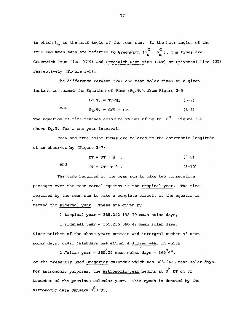
in which h is the hour angle of the mean sun. If the hour angles of the m
true and mean suns are referred to Greenwich (h G h G ), the times are s' m
Greenwich True Time (GTT) and Greenwich Mean Time (GMT) or Universal Time (UT)
respectively (Figure 3-5).
The difference between true and mean solar times at a given
instant is termed the Equation of Time (Eq.T.). From Figure 3-5
Eq.T. = TT-MT (3-7)
and Eq.T. = GTT - UT. (3-8)
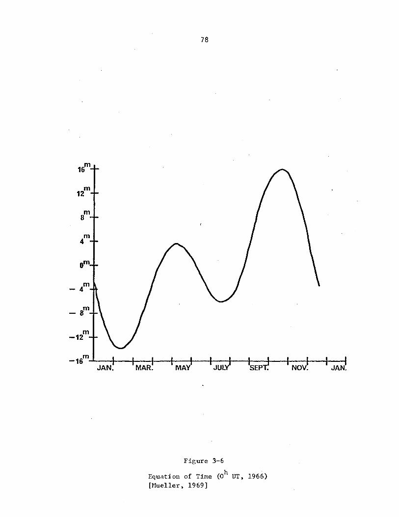
m The equation of time reaches absolute values of up to 16. Figure 3-6
shows Eq.T. for a one year interval.
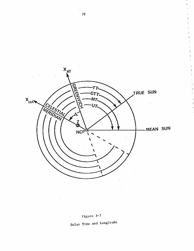
Mean and true solar times are related to the astronomic longitude
of an observer by (Figure 3-7)
MT=UT+A (3-9)
and TT = GTT + A (3-10)
The time required by the mean sun to make two consecutive
passages over the mean vernal equinox is the tropical year. The time
required by the mean sun to make a complete circuit of the equator is
termed the sidereal year. These are given by
1 tropical year = 365.242 198 79 mean solar days,
1 sidereal year = 365.256 360 42 mean solar days.
Since neither of the above years contain and intergral number of mean
solar days, civil calendars use either a Julian yea~ in which
d d h 1 Juliam year = 365.25 mean solar days = 365 6 ,
or the presently used Gregorian calendar which has 365.2425 mean solar days.
For astronomic purposes, the astronomic year begins at Oh UT on 31
December of the previous calendar year. This epoch is denoted by the
d astronomic date January 0.0 UT.
m -12
78
m --16 ~---r---r--~---r---r---r---r---r---r---r---r---r--~
Figure 3-6
Equation of Time (Oh UT, 1966) [Hueller, 1969]
79
Figure 3-7
Solar Ti me and Longitude
TRUE SUN
MEAN SUN
so
corresponding to the Greenwich Sidereal Date (GSD) is the Julian
Date (JD). The"JD is the number of mean solar days that have elapsed
since l2h UT on January 1 (January l~S UT) 4713 Be. For the standard
d astronomic epoch of 1900 January 0.5 UT, JD = 2 415 020.0. The conversions
between GSD and JD are
GSD = 0.671 + 1.00273790~3 JD , (3-11)
JD = -0.669 + 0.9972695664 GSD • (3-12)
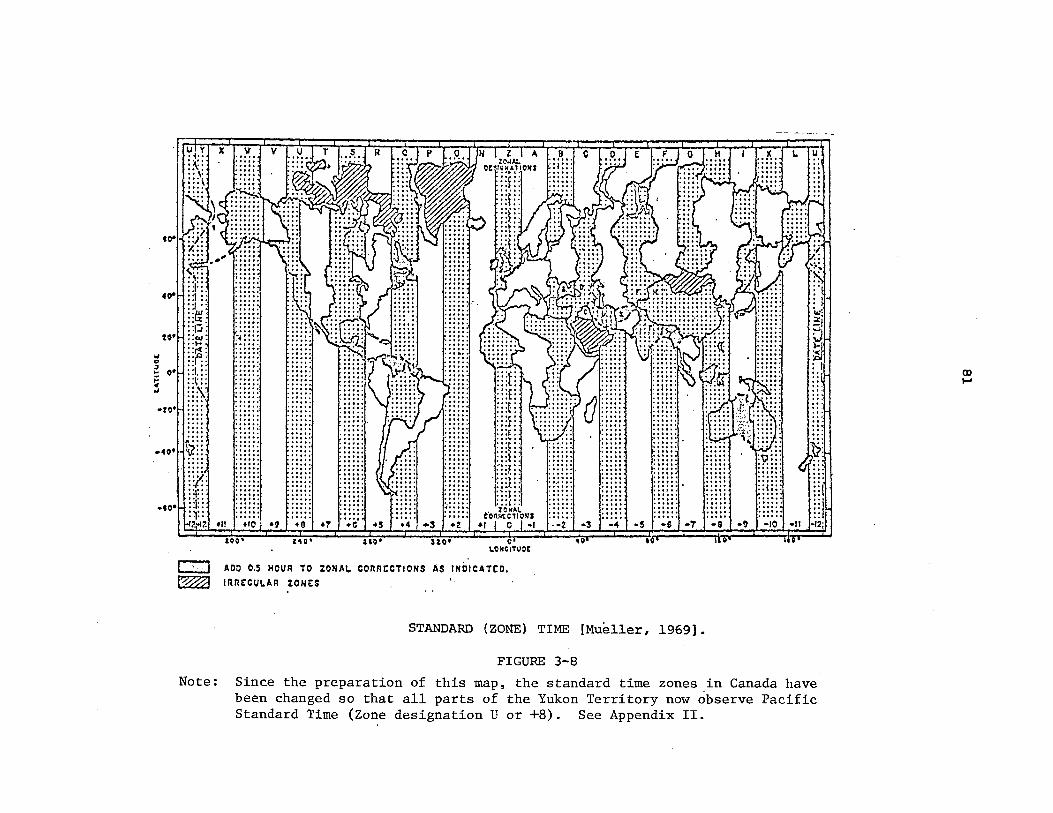
3.2.1 Standard (Zone) Time
To avoid the confusion of everyone keeping the mean time of
their meridian, civil time is based on a "zone" concept. The standard
time over a particular region of longitude corresponds to the mean time
of a particular meridian. In general, the world is divided into 24 zones
of 150 (61\.) each. Zone 0 has the Greenwich meridian as its "standard"
o meridian, and the zone extends 7)2 on either side of Greenwich. The time
zones are numbered -1, -2, •••• , -12 east, and +1, +2, ••• , +12 west.
Note that zone 12 is divided into two parts, 7~°in extent each, on either
side of the International Date Line (lSOoE). All of this is portrayed in
Figure 3-S.
Universal time is related to Zone Time (ZT) by
UT = ZT + liZ , (3-13)
in which liZ is the zonal correction. Care should be taken with liZ,
particularly in regions where summer time or daylight saving time is used
during the spring-summer-fall parts of the year. The effect is a lh
advance of regular ZT.
3.3 Relationships Between Sidereal and Solar Time Epochs and Intervals
We will deal first with the relationship between time epochs.
40"
20"
o·
••• t, • . ,.,t.
...... ;'::::1
,. ~ .. •• & ~ .... .....
-zo'H: : OIl. ...
-40'
·co·
. . ., ...
i;?:: I:
I *t.,.
. , ... "0; .9 +0
100' '10'
t. .... I:· .. · ~ ....
• 1 (;(;' .5
no'
.4 1+3
."5. ..... ., ... ... ". • •• C ••
•• ,tt.
~;::: ;
+2
ao'
: ;:t: : ::E: :::~: :: :::F
~f.l\~. ~'d:: :~:~: : '::c:
t'on~ t:It.O"l S +, J I) I·! Q
t.ONG1Tu~t
;;.:::": .. " '1 ·-2
I: I f, 1 E I:
-3 f -4
40
-5
...... . ..... ~ . "'" _",t' .t"t_ ::::: :' .' .... l It,-'t. .. , .. . ... , .. • • t • ~. ~ •••••• 1
::::::,' ! ... . ...... . .. . ... . ... . .... ·s 1-1
c::J ADO 0.5 HOUR TO ZONAl. COnneCTIons AS INDICATEO.
~ IAIlECUt.AR ZONES
STANDARD (ZO~~) TIME {Mueller, 1969].
FIGURE 3-8
;~ ... :: I • " ~ • e .. , .. ..... .., ...
-K~i ,\t .
..' . : :l~ , .. ::\ ::1
·12'
Note: Since the preparation of this map, the standard time zones in Canada have been changed so that all parts of the Yukon Territory now observe Pacific Standard Time (Zone designation U or +8). See Appendix II.
(0 I-'
Equation (3-6) states
82
MT = 12h + h . , 111
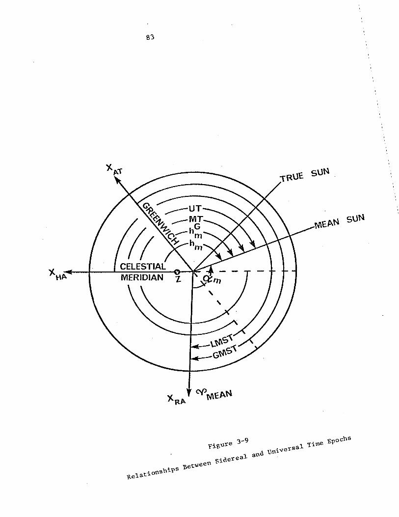
where hm is the hour angle of the mean sun while from' Figure 3-9
which yields
or
h LMST = NT + (am - 12 )
(3-14)
(3-15)
(3-16)
Equations (3-15) and (3-16) represent the transformations of LMST to MT and
vice-versa respectively. G
If we replace MT,hm, and LMST with GMT,nm ' and.
GMST respectively, then
or = GMST - (3-17)
and· GMST= UT + (3-18)
.. - --.
For practical computations we used tabulated quantities. ..... h . -
For example-c- (am -. ·12 ). is tabulated in the Astronomcal Almanac (AA) ;_.
and the quantity' (am ">12h + Eq.· E) is tabulated in the
Star Almanac for Land Surveyors (SALS). Thus for simplicity we should
always convert MT to UT and LMST to GMST. We should note. of course, that the
relationships shown (3-15), (3-16), (3-17), (3-18) relate mean solar and
mean sidereal times. To relate true solar time with apparent sidereal time:
(i) . compute mean solar time (MT = TT - Eq.T or OT = GTT - Eq.T.),
(ii) compute mean sidereal time «3-16) or (3-18»,
(iii) compute apparent sidereal time (LAST = Eq.E + LMST or GAST =
• Eq.E. + GMST).
To relate apparent sidereal time with true solar time, the inverse procedure
is used. For illustrative purposes, two numerical examples are used.
,
,
,
83 ,
, , ,
,
, ,
, ,
, ,
, , ,
, ,
, ,
, , ,
'figure 3-9 n g~de~ea1 and un~~e~sa1 ~ime ~poc~s
~e1at~ons~~Ps ~et~ee •
S4
(note that the
appropriate tabulated values can be found in Figures 3~lO, 3-11, 3-12,
and 3-13).
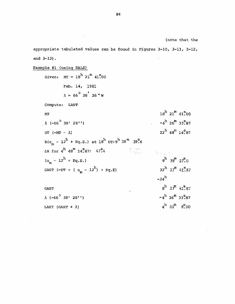
Example #1 (using SALS)
Given: MT = ISh 21m 4l~OO
Feb. 14, 1981
II. = 66 0 3S- 2S" W
compute: LAST
MT Ish 21m 4l~OO
A (_66 0 3S' 28")
UT (=MT - II.)
h h h m s R(a - 12 + Eq.E.) at IS UT:9 38 .39.6
m
~R for 4h 4Sm l4~S7: 47~4 h
(a - 12 + Eq.E.) m
GAST (=UT + ( am - 12h) + Eq.E)
GAST
11. (_66 0 38' 2S")
LAST (GAST + II.)
- -, ..: :~' ~~:. ::---.-: ~
"'4h 26m 33~S7
22h 4Sm l4~87
gh 3f' 27~O 32h -2m 41~87
_24h
sh 2f1 41~87 _4h 26m 33~S7
4h .Om 8~OO
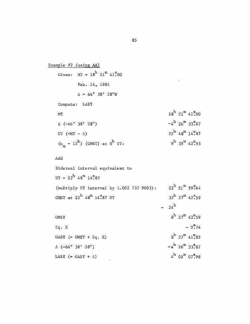
Example #2 (using AA)
h m s Given: MT = 18 21 41.00
Feb. 14, 1981
A = 66° 38' 28"W
Compute: . LAST
MT
A (-66° 3S' 2S")
UT (=MT - A)
(a - l2h) (GMST) at Oh UT: m
Add
Sidereal interval equivalent to
85
(multiply UT interval by 1.002 737 9093):
GMST at 22h 4Sm 14~S7 UT
GMST
Eq. E
GAST (= GMST + Eq. E)
A (-66° 3S' 2S")
LAST (= GAST + A)
ISh 21m 4l~00
-4h 26m 33~S7
22h 4Sm l4~87
9h 35m 42~95
22h 51m 59~64
32h 27m 42~59
24h
8h 27m 42~59
- 0~74
Sh 27m 4l~S5
- 4h 26m 33~S7
4h 01m 07~9S
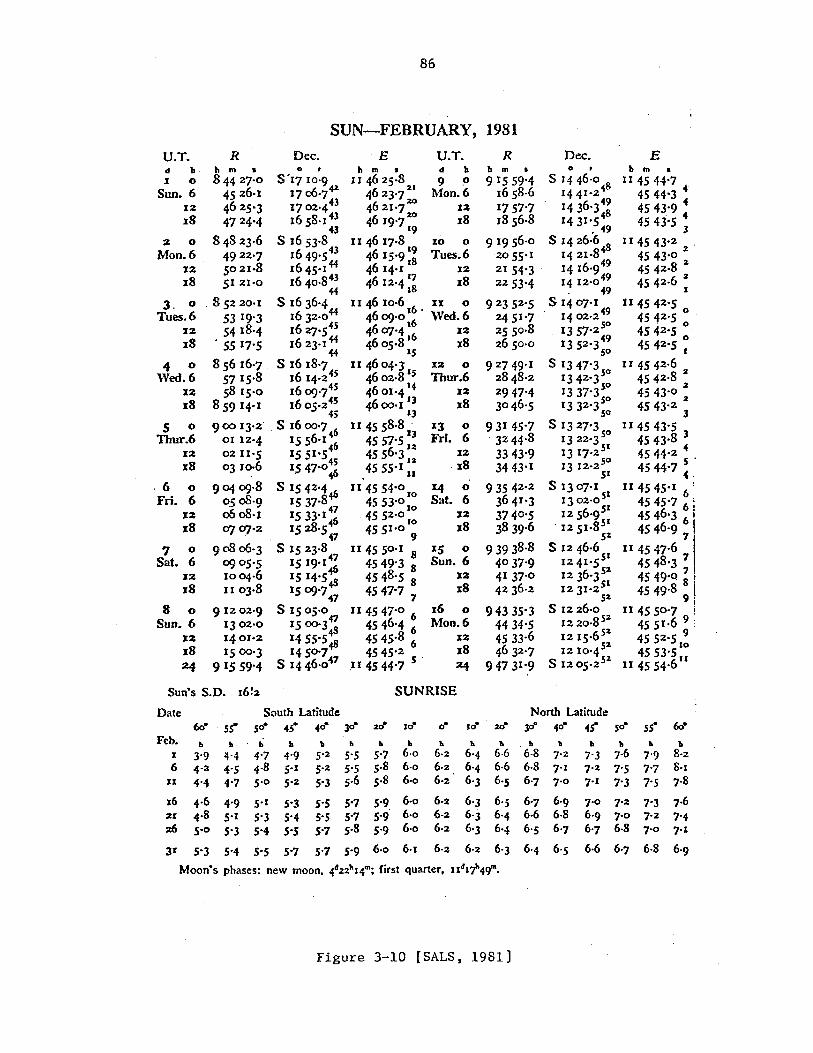
86
SUN-FEBRUARY, 1981
U.T. eI it 1 0
R Dec. 'E U.T. R Dec, E
Sun. 6 12 18
2 0 Mon. 6
][2
18
3. 0 Tues. 6
:1[2
18
... 0 Wed. 6
ll2 ](8
5 0 Thur.6
%2 %8
.6 0
Fri. 6 %2 IS
'1 0 Sat. 6
%2 x8
8 0
Sun. 6 X2 ](8
24
ta rn S
844 27.0
45 26•1
4625'3 47 24-4
84823,6 49 22-7 5021 •8 51 21-0
. 85220- 1
53 19'3 54 18'4
. 55 17-5
85616'7 . 57 IS-S 58 15-0
859 14.1
900 13'2
01 12'4 02 n·s 03 10•6
904 09,8 05 08-9 06 08'1 Cfl Cfl'2
9 0806'3 09 oS'S 1004-6 II °3.8
9 1202-9 13°2 '° 14 01 •2
.15 00'3 9 IS 59'4
Sun's S.D. I6!:e
II m, eI II II 4625,8 9 ~
4623'721 Mon. 6
462I '7 2O
4619'7 20 19
12
%8
II 46 17·8 10 0
4615'91: Tues.6 4614'11 X2
46 12-4:~ %8 II 46 10-6 6 xx 0
4609'016' Wed.6 46 0'.7-1 16 %2 4605.81 %8
IS II 4604',3' X2 0
4602•8 IS Thur.6 4601'414 4600'1 13
13
12 18
II 45 58.8' X3 0
45 57-5 :! Fri. 6 4556'3 x:z
u 8 45 5S'! II . X
114554'0 10
4553'0 10
. 45 p·o 10
4551 •0 9
II 45 50 '1 8 4,5 49'3 8 4548'5 8 4547-7 7
II 45 47'° 6 4546'4 6 4545.8 6 4545'2
.114544" s
X"I 0 Sat. 6
J2 x8
IS 0 Sun. 6
%2 %8
](6 0
Mon. 6
SUNRISE
b m •
9 IS 59'4 1658.6 1757'7 IS 56-8
9 1956'° 20 55.1 21 54-3 . 2253'4
9 2 352 -5 2451'7 2550 -8 26 5°-0
9 2749- 1 28 48'2
2947'4 3°46'5
931 45-7 . 32 44-8 3343'9 3443- 1
93542 •2
36 41 '3 3740 '5 38 39'.6
93938-8 40 37-9 41 37.0
42 36.2
94335'3 44 34'5 4533-6 46 32 -7
94731-9
It m &
II 45 44'7 4544'3 : 4543'9 .. 4543'5 3
II 45 43.2 . 4543.0 2 45 42 .8 1
4542 •6 2 I
114542 -5 4542 '5 0
45 42 -5 0
4542-5 0 I
II 4542,6 4542 -8 2
4543-0 2
4543-2 2 3
H 45 43'S 4543,8 J 45 44-2 of ,
4544'7 : .
u 4545.1 6' 4545'7 6 i 4546'3 6' 4546'9 I
7 II 4547·6
4548'3 7
45 49'0 ~ f 4549-8 !
9j
II 455°'7 4551•6 9 4552 '5 9 4553-5'°
II 45 54.6 "
Date South Latitude North Latitude 00· . 51" so· 1ft' 40· .10" 20· JO· o· .o',·:we )0" 40· 'U- 50" 55° 60"
Feb. x 6.
I> II II '" 3'9 IH 4'7 4'9 4.2 4'5 4,g S-l{ 4-4 4-7 S·o 5-2
4-6 4-9 s-! 5'3 ;,u: 4.8 5.1 5-3 5'4 :7;6 S'O 5-3 5-4 5-5
JI 5'3 S-4 S'S 5-7
II " h .. h 5'2 5-5 5-7 6·0 6,2 5'2 S'S 5.8 6-0 6-2 S-3 5.6 5.8 6'0 6,2
S'S 5'5 5-7
5-7 5'9 6'0 6·2 5-7 5'9 6-0 6,2 5.8 5'9 6-0 6·2,
" h." , 6-4 6·6 6·8 7'Z 6'4 6-6 6·8 7'1 6'3 6'5 6'7 7'0
it h '" iii 7'3 7·6 7'9 8'2 7-2, 7-5 7-7 8,1 7'1 7'3 7'S 7·8
6-3 6·S 6'7 6'9 7-0 7.2 7'3 7.6 6'3 6-4 6·6 6·8 6'9 7-0 7';: 7'4 6'3 6'4 6·S 6'7 6-7 6·8 7-0 "1
S'7 5'9 6·0 6·1 6'2 6'2 6'3 6-4 6·S 6·6 6'7 6·8 6'9
F:igUrE! 3-10 [SALS, 1981]
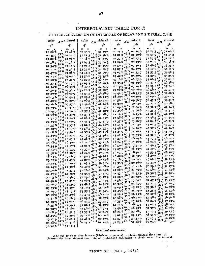
87
INTERPOLATION TABLE :FOR R MUTUAL CO);VERSION OF INTERVALS OF SOLAR AND SIDEREAL TJ:l..JE
sol31" LI R sidereal J solar LJR sidereal
4b 4b 4b 4b
solar LJR sidereal
5b 5h
solar LJR sidereal Sb Sb
In cr;lir(l/ C'(l;I.'S muntl.
Add.1R to s.olar time intt"n' .. l (It"ft-hJnd argument) to oh1 .. in sidereal time inlaya!. Subtract 111< from sidereal time intcn'"l (ril(ht-h:md argument) to obtain sob. time inten'al,
FIGURE 3-11 [SALS,. 1981]
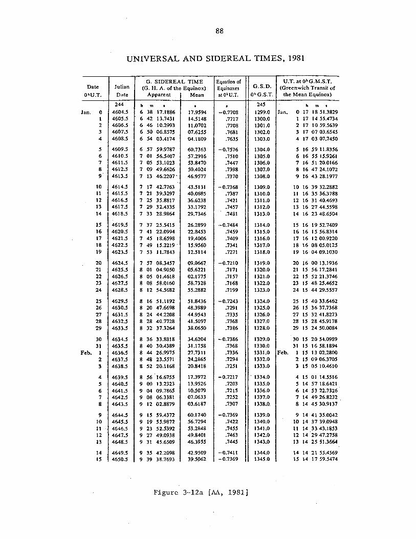
88
UNIVERSAL AND SIDEREAL TIMES, 1981
G. SIDEREAL TIME Equation of I U.T. at OhG.M.S.T. Date Julian (G. H. A. of the Equinox) Equinoxes G. S. D. I (Greenwich Transit of
ObU.T. Date Apparent Mean atOhU.T. OhG.S.T. the Mean Equinox)
244 b m • • • 245 h m • Jan. 0 4604.5 6 38 17.1886 17.9594 -0.7708 1299.0 Jan. 0 17 1851.3829
1 4605.5 6 42 13.7431 14.5148 .7717 1300.0 1 17 1455.4734 2 4606.5 6 46 10.2993 11.0702 .7708 1301.0 2 17 10 59.5639 3 4607.5 6 50 06.8575 07.6255 .7681 1302.0 3 17 0703.6545 4 4608.5 6 54 03.4174 04.1809 .7635 1303.0 4 17 0307.7450
5 4609.s 6 .57 59.9787 60.7363 -0.7576 1304.0 S 16 59 11.8356 6 4610.5 7 01 56.5407 57.2916 .7510 1305.0 6 16 55 15.9261 7 4611.5 7 05 53.1023 53.8470 .7447 1306.0 7 16 5120.0166 8 4612.5 7 09 49.6626 50.4024 .7398 1307.0 8 16 47 24.1072 9 4613.5 7 13 46.2207' 46.9577 .7370 1308.0 9 16 43 28.1977
10 4614.5 7 17 42.7763 43.5131 -0.7368 1309.0 10 16 39 32.2882 11 4615.5 7 21 39.3297 40.0685 .7387 1310.0 11 16 3536.3788 12 4616.5 7 25 35.8817 36.6238 .7421 1311.0 12 16 31 40.4693 13 4617.5 7 29 32.4335 33.1792 .7457 1312.0 13 16 2744.s598 14 4618.5 7 33 28.9864 29.7346 .7481 1313.0 14 16 2348.6504
IS 4619.5 7 37 25.5415 26.2899 -0.7484 1314.0 15 16 19 52.7409 16 4620.5 7 41 22.0994 22.8453 .7459 1315.0 16 16 15 56.8314 17 462l.S 7 45 18.6598 19.4006 .7409 1316.0 17 16 12 00.9220 18 4622.5 7 49 15.2219 . t5.9560 .7341 1317.0 18 16 0805.0125 19 4623.5 7 53 11.7843 12.5114 .7271 1318.0 19 16 0409.1030
20 4624.5 7 57 08.3457 09.0667 -0.7210 1319.0 20 16 00 13.1936 21 4625.5 8 01 04.9050 05.6221 .7171 1320.0 21 IS 56 17.2841 22 4626.5 8 05 01.4618 02.1775 .7157 1321.0 22 15 5221.3746 23 4627.5 8 08 58.0160 58.7328 .7168 1322.0 23 15 48 25.4652 24 4628.5 8 12 54.5682 55.2882 .7199 1323.0 24 15 4429.5557
25 4629.5 8 16 51.1192 51.8436 -0.7243 1324.0 25 15 4033.6462 26 4630.5 8 20 47.6698 48.3989 .7291 1325.0 26 15 3637.7368 27 4631.5 8 24 44.2208 44.9543 .7335 1326.0 27 15 3241.8273 28 4632.5 8 28 40.7728 41.5097 .7368 1327.0 28 15 2845.9178 29 4633.5 8 32 37.3264 38.0650 .7386 1328.0 29 IS 24 50.0084
30 4634.5 8 36 33.8818 34.6204 -0.7386 1329.0 30 15 2054.0989 31 4635.5 8 40 30.4389 31.1758 .7368 1330.0 31 15 1658.1894
Feb. I 4636.5 8 44 26.9975 27.7311 .7336 1331.0 Feb. • 15 1302.2800 2 4637.5 8 48 23.5571 24.2865 .7294 1332.0 2 15 09 06.3705 3 4638.5 8 52 20.1168 20.8418 .7251 1333.0 3 15 05 10.4610
4 4639.5 8 56 16.6755 17.3972 -0.7217 . 1334.0 4 15 0 I 14.5516 5 4640.5 .9 00 13.2323 13.9526 .7203 1335.0 5 14 57 18.6421 6 4641.5 9 04 09.7865 10.5079 .7215 1336.0 6 14 53 22.7326 7 4642.5 9 08 06.3381 07.0633 .7252 1337.0 7 14 49 26.8232 8 4643.5 9 12 02.8879 03.6187 .7307 .1338.0. 8 14 45 30.9137
9 4644.5 9 15 59.4372 60.1740 -0.7369 1339.0 9 14 41 35.0042 10 4645.5 9 19 55.9872 56.7294 .7422 1340.0 10 14 3739.0948 11 4646.5 9 23 52.5392 53.2848 .7455 1341.0 II 14 33 43.1853 12 4647.5 9 27 49.0938 49.8401 .7463 1342.0 12 142947.2758 13 4648.5 9 31 45.6509 46.3955 .7445 1343.0 13 14 25 51.3664
14 4649.5 9 35 42.2098 42.9509 -0.74t1 1344.0 14 14 21 55.4569 IS 4650.5 9 39 38.7693 39.5962 -0.7369 1345.0 15 14 17 59.5474
Figure 3-12a [AA, 1981]

89
UNIVERSAL AND SIDEREAL TIMES p 1981
G. SIDEREAL TIME Equation of U.T. at OhG.M.S.T. Date Julian (G. H. A. of the Equinox) Equinoxes G.S.D. (Greenwich Transit of
OhU.T. Date Apparent Mean at O~U.T. O'G.S.T. tbe Mean Equinox)
244 h m • • • 245 , . m • Feb. 15 4650.5 9 39 38.7693 39.5062 -0.7369 1345.0 Feb. 15 14 1759.5474
16 4651.5 9 43 35.3282 36.0616 .7334 1346.0 16 14 1403.6380 17 4652.5 9 47 31.8854 32.6169 .7315 1347.0 17 14 1007.7285 .18 4653.5 9 51 28.4403 29.1723 .7320 1348.0 18 14 0611.8191 19 4654.5 9 55 24.9927 25.7277 .7350 1349.0 19 14 02 15.9096
20 4655.5 9 59 21.5429 22.2830 -0.7401 1350.0 20 13 58 20.0001 21 4656.5 10 03 18.0916 18.8384 .7468 1351.0 21 13 54 24.0~07 22 4657.5 10 07 14.6396 15.3938 .7541 1352.0 22 13 5028.1812 23 4658.5 10 11 11.1878 11.9491 .7613 1353.0 23 13 4632.2717 24 4659.5 10 15 07.7369 08.5045 .7676 1354.0 24 13 42 36.3623
25 4660.5 10 19 04.2874 05.0599 -0.7725 1355.0 25 13 38 40.4528 26 4661.5 10 23 00.8396 01.6152 .7756 1356.0 26 13 34 44.5433 27 4662.5 10 26 57.3936 58.1706 .7770 1357.0 27 t3 30 48.6339 28 4663.5 10 30 53.9492 54.7260 .7768 1358.0 28 13 2652.7244
Mar. 1 4664.5 10 34 50.5059 51.2813 .7754 1359.0 Mar. I 13 2256.8149
2 4665.5 10 38 47.0631 47.8367 -0.7735 1360.0 '2 13· 1900.9055 3 4666.5 10 42 43.6199 44.3921 .7721 1361.0 3 13 1504.9960 4 4667.5 10 46 40.1753 40.9474 .7721 1362.0 4 13 11 09.0865 5 4668.5 10 50 36.7284 37.5028 .7743 1363.0 5 t3 07 13.1771 6 4669.5 10 54 33.2790 34.0581 .• 7792 1364.0 6 t3 03 17.2676
7 4670.5 10 58 29.8272 30.6135 -0.7863 . 1365.0 7 12 5921.3581 8 4671.5 11 02 26.3744 27.1689 .7945 1366.0 8 12 5525.4487 9 4672.5 11 06 22.9220 23.7242 .8022 1367.0 9 12 51 29.5392
10 4673.5 11 10 19.4715 20.2796 .8081 1368.0 10 12 47 33.6297 11 4674.5 11 14 16.0238 16.8350 .8112 1369.0 II 12 4337.7203
12 4675.5 11 18 12.5788 13.3903 -0.8115 1370.0 12 12 3941.8108 13 4676.5 11 22 09.1358 09.9457 .8099 1371.0 13 12 35 45.9013 14 4677.5 11 26 05.6937 06.5011 .8074 1372.0 14 12 31 49.9919 15 4678.5 11 30 02.2512 03.0564 .8053 1373.0 IS 12 27 54.0824 16 4679.5 11 33 58.8072 59.6118 .8046 1374.0 16 12 23 58.1729
17 4680.5 11 37 55.3611 56.1672 -0.8060 1375.0 17 12 2002.2635 18 468t.S 11 41 51.9127 52.7225 .8098 1376.0 18 12 1606.3540 19 4682.5 II 45 48.4621 49.2779 .8158 1377.0 19 12 1210.4445 20 4683.5 11 49 45.0099 45.8333 .8234 1378.0 20 12 08 14.5351 21 4684.5 11 53 4t.S568 42.3886 .8318 1379.0 21 12 04 18.6256
22 4685.5 11 57 38.1038 38.9440 -0.8402 1380.0 22 12 0022.7161 23 4686.5 12 01 34.6515 35.4993 .8478 1381.0 23 II 5626.8067 24 4687.5 12 OS 31.2006 32.0547· .854l 1382.0 24 11 5230.8972 25 4688.5 12 09 27.7515 28.6101 .8586 1383.0 2511 4834.9877 26 4689.5 12 13 24.3042 25.1654 .8613 1384.0 26 11 4439.0783
27 4690.5 12 17 20.8585 21.7208 -0.8623 1385.0 2711 4043.1688 28 4691.5 12 21 17.4142 18.2762 .8619 1386.0 28 It 3647.2593 29 4692.5 12 25 13.9707 14.8315 .8609 1387.0 29 II 3251.3499 30 4693.5 12 29 10.5270 tl.3869 .8599 1388.0 30 II 2855.4404 31 4694.5 12 33 07.0825 07.9423 .8597 1389.0 31 11 2459.5309
Apr. 1 4695.5 12 37 03.6363 04.4976 -0.8614 1390.0 Apr. 1 11 2103.6215 2 4696.5 12 41 00.1877 01.0530 -0.8653 1391.0 2 11 1707.7120
Figure 3-12h [AA, 1981]
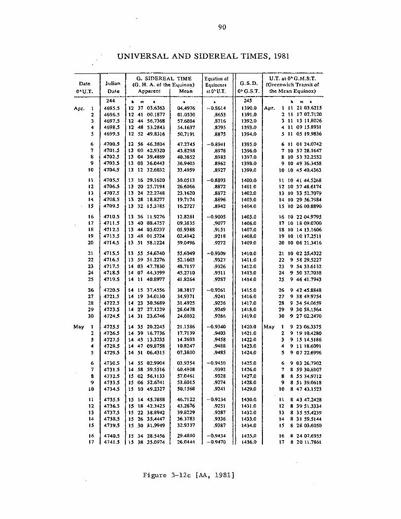
90
UNIVERSAL AND SIDEREAL TIMES. 1981
G. SIDEREAL TIME Equation or U.T. at OhG.M.S.T. Date Julian (G. H. A. or the Equinox) Equinoxes G.S.D. (Greenwich Transit or
OhU.T. Date Apparent Mean aIOhU.T. OhG.S.T. the Mean Equinox)
244 b m • • • 245 b ... • Apr. 1 4695.5 12 37 03.6363 04.4976 -0.8614 1390.0 Apr. I 11 21 03.6215
2 4696.5 12 41 00.1877 01.0530 .8653 1391.0 2 11 1707.7120 3 4697.5 12 44 56.7368 57.6084 .8716 1392.0 3 II 13 11.8026 4 4698.5 12 48 53.2843 54.1637 .8795 1393.0 4 II 09 15.8931 5 4699.5 12 52 49.8316 50.7191 .8875 1394.0 5 \I OS 19.9836
6 47005 12 56 46.3804 47.2745 -0.8941 1395.0 6 II 01 24.0742 7 4701.5 13 00 42.9320 43.8298 .8978 1396.0 7 10 5728.1647 8 4702.5 13 04 39.4869 40.3852 .8983 1397.0 8 10 53 32.2552 9 4703.5 13 OS 36.0443 36.9405 .S962 1398.0 9 10 49 36.345S
10 47045 13 12 32.6032 33.4959 .8927 1399.0 10 10 45 40.4363
11 4705.5 13 16 29.1620 30.0513 -0.8893 1400.0 11 10 41 44.5268 12 4706.5 13 20 25.7194 ~6.6066 .8872 1401.0 12 10 3748.6174. 13 4707.5 13 24 22.2748 23.1620 .8872 1402.0 13 10 33 52.7079 14 4708.5 13 28 18.8277 19.7174 .8896 1403.0 14 10 29 56.7984 IS 4709.5 13 32 15.3785 16.2727 .8942 1404.0 IS 10 2600.8890
16 4710.5 13 36 11.9276 12.8281 -0.9005 1405.0 16 10 22 04.9795 17 4711.5 13 40 08.4757 09.3835 .9077 1406.0 17 10 180.9.0700 18 4712.5 13 44 05.0237 05.9388 .9151 1407.0 18 10 14 13.1606 19 47135 13 48 01.5724 02.4942 .9218 140S.0 19 10 1017.2511 20 4714.5 13 51 58.1224 59.0496 .9272 1409.0 20 10 06 21.3416
21 4715.5 13 55 .54.6740 55.6049 -0.9309 1410.0 21 10 02 25.4322 22 4716.5 13 59 51.2276 52.1603 .9327 1411.0 22 9 5829.5227 23 4717.5 14 03 47.7830 4S.7157 .9326 1412.0 23 9 5433.6132 24 4718.5 14 07 44.3399 45.2710 .9311 1413.0 24 9 5037.7038 25 4719.5 14 11 40.8977 41.8264 .9287 1414.0 2.S 9 4641.7943
26 4720.5 14 15 37.4556 38.3817 -0.9261 1415.0 26 9 4245.8848 27 472t.S 14 19 34.0130 34.9371 .9241 1416.0 27 9 3849.9754 2S 4722.5 14 23 30.5689 31.4925 .9236 1417.0 28 9 3454.0659 29 4723.5 14 27 27.1229 28.0478 .9249 1418.0 29 9 3058.1564 30 4724.5 14 31 23.6746 24.6032 .9286 1419.0 30 9 2702.2470
May 1 4725.5 14 35 20.2245 21.1586 -0.9340 1420.0 May 1 9 2306.3375 2 4726.5 14 39 16.7736 17.7139 .9403 1421.0 2 9 1910.4280 3 4127.5 14 43 13.3235 14.2693 .9458 1422.0 3 9 15 14.5186
" 4728.5 14 47 09.8758 10.8247 .9488 1423.0 4 9 11 18.6091 5 4129.5 14 51 06.4315 07.3800 .9485 1424.0 S .9 07 22.6996
6 4730.5 14 55 02.9904 03.9354 -0.9450 1425.0 6 9 0326.7902 7 4731.5 14 58 59.5516 60.490S .9392 1426.0 7 8 5930.8807 8 4732.5 15 02 56.1133 57.0461 .9328 1427.0 8 8 5534.9712 9 4733.5 IS 06 52.6741 53.6015 .9274 1428.0 9 8 51 39.0618
10 4734.5 IS 10 49.2327 50.1568 .9241 1429.0 10 8 4743.1523
11 4735.5 IS 14 45.7888 46.7122 -0.9234 1430.0 " 8 4347.2428 12 4736.5 IS 18 42.3425 43.2676 .925' 1431.0 12 8 3951.3334 13 4737.5 IS 22 38.8942 39.8229 .9287 1432.0 13 8 3555.4239 14 4738.5 IS 26 35.4447 36.3783 .9336 1433.0 14 8 31 59.5144 15 4739.5 IS 30 31.9949 32.9337 .9387 1434.0 IS 8 2803.6050
16 4740.5 IS 34 28.5456 29.4890 -0.9434 1435.0 16 8 2407.6955 17 4741.5 IS 38 25.0974 26.0444 -0.9470 1436.0 17 8 2011.7S61
Figure 3-12c [AA, 1981]
91
We now turn our attention to the relationship of the sidereal
and solar time intervals. The direction of the sun in space, relative to
the geocentre, varies due to the earth's orbital motion about the sun. The
result is that the mean solar day is longer than the mean sidereal day by
approximately 4 minutes. After working out rates of change per day, one
obtains
ld (5) = 23h 56m 04~09054 (M) , ~d (M) = 24h 03m 56~55536 (5),
lh (5) = 59m 50~17044 (M) , Ih (M) = 1h OOm 09~85647 (5),
1m (5) = 59~83617 (M) , 1m (M) = Olm OO~l6427 (5),
1s (5) s
eM) IS (M)· = Ol~OO273 (5), = . 0.99727 ,
in which 5 and M refer to mean sidereal· and mean solar times respectively.
These numbers are derived from the fact that a tropical (solar) year contains
366.2422 mean sidereal day~ or 365.2422 mean so~ar days. The ratio·s.are
then
mean solar time interval = (365.2422/366.2422) = 0.997 269 566 4x mean
sidereal time interval,
mean sidereal time interval = (366.2422/365.2422) = 1.002 737 909x
mean solar time interval.
The usefulness of a knowledge of the intervals is given in the following
numerical example.
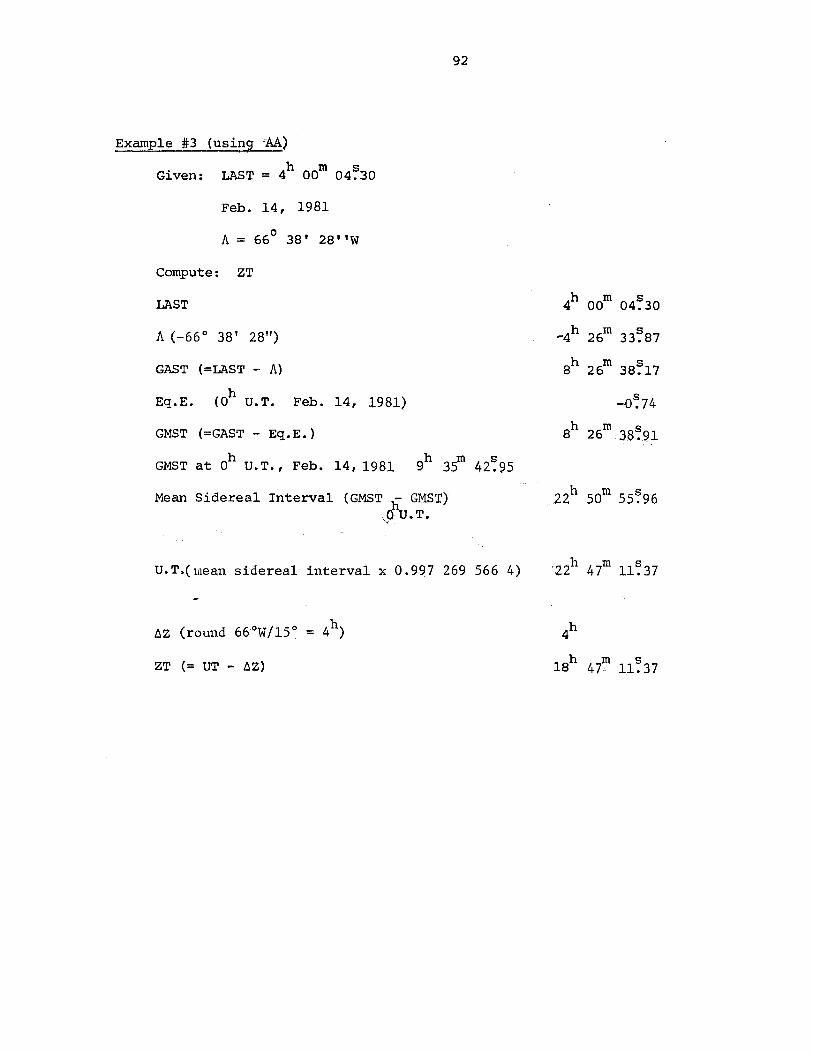
92
Example #3 (using 'M)
Given: LAST = 4h OOm 04~30
Feb. 14, 1981
A = 66° 3S' 2S"W
compute: ZT
LAST 4h Oom 04~30
A (-66 0 38' 28")
GAST (=LAST - A)
h Eq.E. (0 U.T. Feb. 14, 1981)
GMST (=GAST - Eq.E.)
GMST at Oh U.T., Feb. 14, 1981· 9h 3? 42:95
Mean Sidereal Interval (GMST ii GMSTl ,,(,LU. T.
U.T.(mean sidereal interval x 0.997 269 566 4)
ZT (= UT - ~Z)
"4h 26m 33~S7
Sh 26m 3S~17
-{)~74
Sh 26m 38~9l
4h
lsh 47'1'f1ll~37
93
3.4 Irregularities of Rotational Time Systems
Sidereal and Universal time systems are based on the rotation of
the earth; thus, they are subject to irregularities caused by (i) changes
in the rotation rate of the earth, we' and (ii) changes in the position of
the rotation axis (polar motion). The differences are expressed in terms
of Universal time as follows:
UTa is UT deduced from observations, is affected by changes in W e
and polar motion, thus is an irregular time system.
UTI is defined as UTa corrected for polar motion, thus it represents
the true angular motion of the earth and is the system to be
used for geodetic astronomy (note that it is an irregular time
system due to variations in w·) • e
UT2 is defined as UTI corrected for seasonal variations in w . This e
time system is non-uniform because w is slowly decreasing due e
to the drag of tidal forces and other reasons.
UTC Universal Time Coordinated is the internationally agreed upon
time system which is transmitted by most radio time stations.
UTC has a defined relationship to International Atomic Time
(IAT), as well as .. to UT2 and to UTI.
More information on UTe, UTI, and UT2, particularly applicable
to timekeeping for astronomic purposes, is given in chapter 4.
3.5 Atomic Time System
Atomic time is based on the electromagnetic oscillations
produced by the quantum transition of an atom. In 1967, the International
committee for Weights and Measures defined the atomic second (time interval)
as "the duration of 9 192 631 770 periods of radiation corresponding to
94
the transition between the two hyper-fine levels of the fundamental state
of the atom of Caesium 133"jRobbins, 1976J. Atomic frequency standards
are the most acurate standards in current use with stabilities of one or
. 1012 d '1" f . 1014 b . d two parts ~n common, an stab~ ~t~es 0 two parts ~n a ta~ne
from. the mean of sixteen specially selected caesium standards at ·the us
Naval Observatory.
Various atomic time systems with different epochs are in use.
The internationally accepted one is called International Atomic Time,
which is based on the weighted means of atomic clock systems. throughout the
world. The work required to define IAT is carried out by BIH (Bureau
International de l'Heure) in Paris IRobbins, 1976]. IAT, through its
relationship with UTC, is the basis for radio broadcast time signals.
4. TIME DISSEIUNATION, TIME-KEEPING, TIME RECORDING
4.1 Time Dissemination
As has been noted several times already, celestial coordinate
systems are subject to change with time. To make use of catalogued
positions of celestial bodies for position and azimuth determination at
any epoch, we require a measure of the epoch relative to the catalogued
epoch. In the interests of homogeneity, it is in our best interest if on
a world-wide bases everyone uses the same time scale.
Time signals are broadcast by more than 30 stations around the
world, with propagation frequencies in either the HF (1 to 50 MHz) or LF
(10 to 100 KHz) ranges. The HF (high frequency) tend to be more useful
for surveying purposes as a simple commercial radio receiver can be used.
The LF (low frequency) signal are more accurate since errors due to
propagation delay can be more easily accounted for.
In North America, the two most commonly used time signals are
those broadcast by WWV, Boulder, Colorado (2.5 MHz,S MHz, 10 MHz, 15 MHz,
20 MHz) and CHU, Ottawa (3.330 MHz, 7.335 MHz, 14.670 MHz).
The broadcast signal is called Universal Time Coordinated (UTC).
UTC is a system of seconds of atomic time, that is IS UTC is lSAT to the
accuracy of atomic time and it is constant • h '.At 1972 January lOUT,
. . UTCwas ... deUned . .to. belAT . minus . 1Us .exactly ..... ,w.'Ihe quantit.,y: ~.(l.AT":,,UTC),
called DAT, will always be an integral number due to the introduction of
the "leap second" (see below).
The time we are interested in is UTI. The value, (UTI-UTe) is
denoted DUTI and never exceeds the value 0~9. The value DUTl is predicted
and published by BIH. Precise values are published one month in arear~.
95
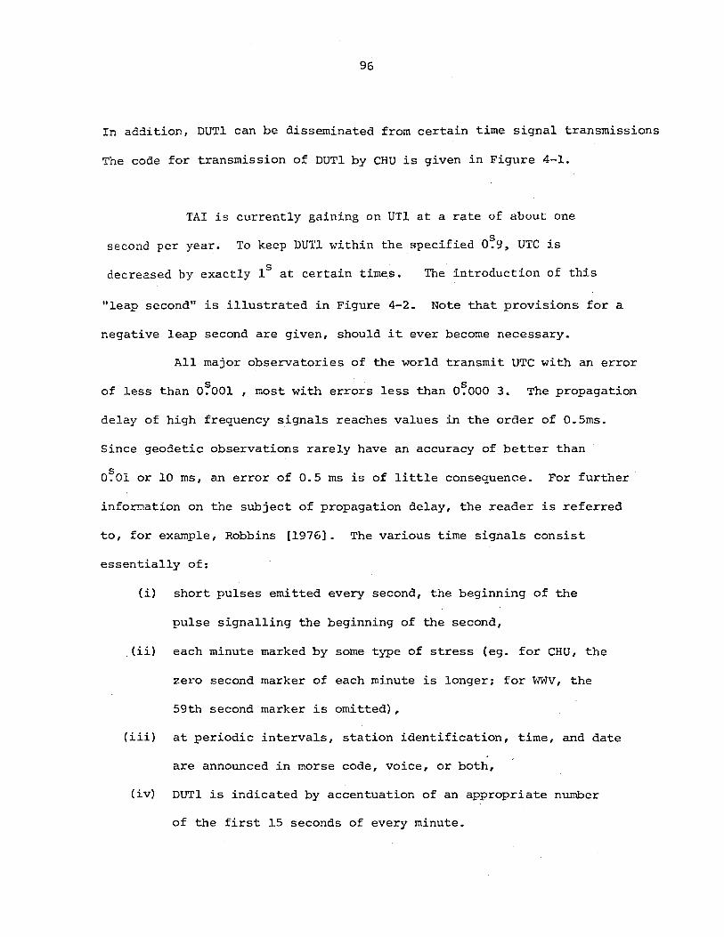
96
In addition, DUTI can be disseminated from certain time signal transmissions
The code for transmission of DUTI by CHU is given in Figure 4-1.
TAl is currently gaining on UTI at a rate of about one
s second per year. To keep DUTI within the specified 0.9, UTe is
decreased by exactly IS at certain time~. The introduction of this
"leap second" is illustrated in Figure 4 ... 2. Note that provisions for a
negative leap second are given, should it ever become necessary.
All major observatories of the world transmit UTC with an error
of less than O~OOI , most with errors less than O~OOO 3. The propagation
delay of high frequency signals reaches values in the order of O.Sms.
Since geodetic observations rarely have an accuracy of better than
s 0.01 or 10 ms, an error of 0.5 ms is of little consequence. For further
information on the subject of propagation delay, the reader is referred
to, for example, Robbins [1976]. The various time signals consist
essentially of:
(i) short pulses emitted every second, the beginning of the
pulse signalling the beginning of the second,
,(ii) each minute marked by some type of stress (eg. for CHU, the
zero second marker of each minute is longer; for wwv, the
59th second marker is omitted)p
(iii) at periodic intervals, station identification, time, and date
are announced in morse code, voice, or both,
(iv) DUTl is indicated by accentuation of an appropriate number
of the first 15 seconds of every minute.
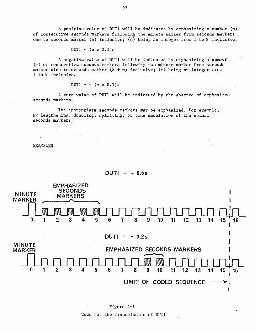
97
A positive value of DUT1 will be indicated by emphasizing a number (n) of consecutive seconds markers following the minute warker from seconds markers one to seconds marker (n) inclusive; (n) being an integer from 1 to 8 'inclusive.
DUT1 = (n x O.l)s
A negative value of DUT1 will be indicated by e~phasizing a'number (m) of consecutive seconds markers following the minute marker from seconds marker nine to seconds marker (8 + m) inclusive; (m) being an integer from 1 to 8 inclusive.
DUT1 = - {m x O.l)s
A zero value of DUTI will be indicated by the absence of emphasized seconds markers •
The appropriate seconds markers may be emphasized, for example, by lengthening, doubling, splitting, or tone modulation of the normal seconds markers.
EXAMPLES
EMPHASIZED MI NUTE SECONDS
MARKERS MARKER , ___ ----A ..... ---..,.,
o
MINUTE M'ARKER
DUTI = + 0.55
DUTI = - 0.25
EMPHASIZED SECONDS MARKERS r-A-.
I I I I
LIMIT OF CODED SEQUENCE --I I
Figure 4-1
Code for the Transmission of DUT1
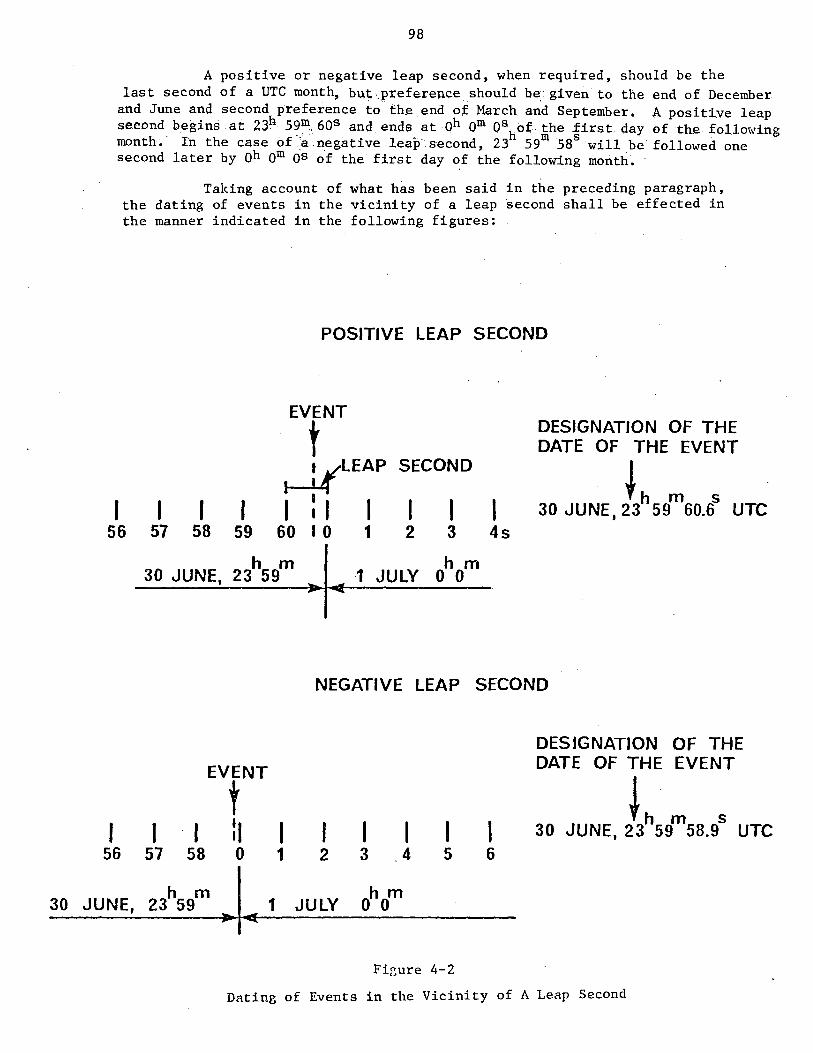
98
A positive or negative leap second, when required, should be the last second of a UTe month, but;,preierenceshould be,' given to the end of December
and June and second preference to the end of March and September. 1(,. positive leap second begins at 23h 59,m. 60S a~d ends.~tOh Om O\of~he ~ir~t day of' the following month~ In the case of anegat1.ve leap second, 23 59 58 w:Lll be followed one second later by Oh Om Os of the first day of the following month ..
. ...
I
Taking account of what h~s been said in t~e preceding paragraph, the dating of events in the vicinity of a leap second shall be effected in the manner indicated in the following figures:
I I
POSITIVE LEAP SECOND
EVENT
t ~lEAP
I : I I
SECOND
I
DESIGNATION OF THE DATE OF THE EVENT
. ~h m s . 30 JUNE, 23 59 60.6 UTe
56 51 58 59 60 I 0 1 2 3 4s
30 JUNE, 23h59m 1 JULY OhOm ~
NEGATIVE LEAP SECOND
DESIGNATION OF THE
EVENT DATE OF THE EVENT
t t m s I I . I a I I I I I 30 JUNE, 23 59 58.9 UTC
56 57 58 0 1 2 3 4 5 6
30 JUNE, 23h59m ~I~ 1 JULY ohom
Fir.;ure 4-2
Dating of Events in the Vicinity of A Leap Second
99
4.2 Time~Keeping and Recording
Time reception, before the advent of radio, was by means of the
telegraph. Since the 1930's, the radio receiver has been used almost
exclusively in geodetic astronomy. Time signals are received and amplified,
after which they are used as a means of determining the exact time of an
observation. Direct comparison of a time signal with the instant of
observation is not made in practice - a clock (chronometer) is used as an
intermediate means of timekeeping. Usually, several comparisons of clock
time with UTe are made during periods when direction observations are not
taking place. The direction obs~rvations are subsequently compared to
clock time.
The most practical receiver to use is a commercial portable
radio with a shortwave (HF) band. In areas where reception is difficult,
a marine or aeronautical radio with a good antenna may become necessary.
The chronometer or clock used should be one that is very stable,
that is, it should have a constant rate. There are three broad
categories of clock that may be used:
(1) Atomic clocks, (2) Quartz crystal clock, (3) Mechanical clock.
Atomic clocks are primarily laboratory instruments, are very
costly, and have an accuracy that is superfluous for geodetic purposes.
Quartz crystal clocks are the preferred clocks. They are portable, stable
(accuracy of 1 part in 107 to 1 part in 1012), but do require a source of
electricity. This type of time-keeper is normally used for geodetic
purposes, in conjunction with a time-recorder, (e.g. chronograph) where
an accuracy of O~OOI or better is required. Mechanical clocks, with
100
accuracies in the order of 1 part in 106 , suffice for many surveying needs
(eg. where an accuracy of O~l is required). They are subject to
mechanical failure and sudden variations in rate, but' they are portable
and independent of an outside source of electricity. The most common and
useful mechanical clock is a stop watch, reading to O~l, with two sweep
seconds hands. One should note that many of the new watches - mechanical,
electronic, quartz crystal - combine the portable-stable criteria and the
stop watch capabilities, and should not be overlooked. With any of these
latter devices, time-recording is manual, and the observing procedure is
audio-visual.
4.3 Time Observations
In many instances, the set of observations made for the astronomic
determination of position and azimuth includes the accurate determination
and recording of time. While in many cases,(latitudeand azimuth
mathematical models and associated star observing programs can be devised
to minimize the effects of random and systematic errors in time, the
errors in time always have a direct effect on longitude (e.g. if time is
s in error by 0.1, the error in A will be 1~'5).
The timekeeping device that is most effective for general
surveying purposes is the stop watch, most often a stop watch with a mean
solar rate (sidereal rate chronometers are available). The five desireable
elements for the stop watch are lRobbins, 1976]:
(i) two sweep seconds hands,
(ii) a start-stop-reset button which operates both hands together,
resetting them to zero,
101
(iii) a stop-reset button which operates on the secondary seconds
hand only, resetting it to coincidence with the main hand
which is unaffected by the operation of this button,
(iv) reading to 0~1,
(v) a rate sufficiently uniform over at least one half an hour
to ensure that linear interpolation over this period does not
s give an error greater than 0.1.
A recommended time observing procedure is as follows [Robbins, 1976]:
(i) start the watch close to a whole minute of time as given by
the radio time signal,
(ii) stop the secondary hand on a whole time signal second, record
the reading and reset. A mean of five readings of time
differences (see below) will give the 6T of the stop watch at
the time of comparison.
(iii) stop the secondary hand the instant the celestral body is in
the desired position in the telescope (this is done by the
observer). Record the reading and reset.
(iv) repeat (iii) as direction observations are made.
(v) m repeat (ii) periodically (at least every 30 ) so that the
clock rate for each time observation· can be determined.
The clock correction (6T) and clock rate (61T) are important
parts of the determination of time for astronomic position and azimuth
determination. Designating the time read on our watch as T, then the
zone time (broadcast, for example, by CHU) of an observation can be
stated as
ZT =·T + t:.T (4-1)
102
In (4-ll! it is assumed that ~T is constant. ~T will usually not be
constant but changes should occur.at a uniform rate, bolT. Then boT is
given by
where
~T,~T are clock corrections at times T, T , o 0
~lT is the change in ~T per unit of time,
the clock (chronometer) rate.
(4-2)
The clock correction, ~T for any time of observation, is determined via
a simple linear interpolation as follows:
(i) using the radio and clock comparisons made before, during, and
after the observing program, compute ~T for each by
~T, = ZT, - T, 1 1 1
(4-3)
(ii) Compute the time difference, boZT, '+1 between time comparisons 1,1
by
~ZTi,i+l = ZTi +l - ZTi (4-4)
(iii) Compute the differences between successive clock corrections
corresponding to the differences ~ZT, '+1 ' namely 1,1.
boT, , 1= ~T '+1- boT, 1.,1.+ 1. 1
(iv) Compute the clock rate per mean solar hour by
~ T = 1
~T, '+1 1,1.
~ZT, '+1 1.,1
tv) Record the results in a convenient and usable form
(e.g. table of values, graph).
(4-5)
(4-6)
103
This time determination process is illustrated by the following example.
Clock Correction and Clock Rate
(i) Determination of ZT of stop watch
ZT (radio) Stop Watch (T) ~T, (Radio-Stop watch) 1
gh 13m OO~O Oh OOm OO~O gh 13m OO~O
13m 15~0 OOm 14~8 gh 13m 00~2
13m 45~0 OOm 45~2 gh 12m 59~8
gh 14m OO~O Oh Olm OO~O gh 13m OO~O
14m 30~0 Olm 29~9 gh 13m 00~1
ZT of beginning = (i~T,)/i = gh 13m oo~b i=l 1
This procedure is to be repeated for each time comparison with
the radio time signal.
(ii) Record of time comparisons; determination of clock rate.
ZT Clock ~ T (radio) (stop watch) ~ZT, '+1 ~T ~T. '+1 (~/h)
TIME (T) 1,1 0 1,1
gh13mOO~O ohOomOO~O Oh28mOO~0
gh13mOO~0
gh41mOO~0 Oh27m59~2 gh13mOO~8 00~8 1.7
10h30mOO~0 Ih16m57~7 Oh49mOO~0
gh13m02~3 01~5 1.8
llh33mOO~0 2h19m55~7 Ih03mOO~0
gh13m04~3 02~0 1.g
104
(iii) Graph of Clock (stop watch) Correction ~T
-t:i -."..,-
•
CLOCK TIME (To)
(iv) Determination of the true zone time of a direction observation.
Observed Time (stop watch):
What is true ZT ?
From the graph: h m s ~T at ZT observed = 9 13 01.6
ZT (true) = Oh S2m 28~8 + gh 13m 01~6
= 10h OSm 30~4
Using ~T = ~To + (Ti +1 - Ti)~lT yields
6T = gh 13m OO~8 + (O~40803) 1.8 = gh 13m Ol~S
ZT(true) = Oh S2m 28~8 + gh 13m 01~6
= 10h OSm 30~3 •
105
In closing this section, the reader is cautioned that the
methods described here for time determination are not adequate for precise
(e.g. first-order) determinations of astronomic azimuth and position. Such
s work requires an accuracy in time of 0.01 or better. For details, the
reader is referred to, for example, Mueller I1969J or Robbins 11976].
5. STAR CATALOGUES AND EPHEMERIDES
5.1 Star Catalogues-
Star catalo9Ues contain the listing of the positions of stars in
a unique coordinate system. The positions are generally given in the mean
right ascension coordinate system for a particular epoch T. Besides o
listing the right ascensions and declinations, star catalogues identify
each star by number and/or name, and should give their proper motions.
Some catalogues also include annual and secular variations. Other
pertinent data sometimes given are estimates of the standard errors of the
coordinates and their variations, and star magnitudes. (Magnitude is an
estimate of a star's brightness given on a numerical scale varying from
-2 for a bright star to +15 for a dim star).
There are two main types of catalogues: (i) Observation
catalogues containing the results of particular observing programs, and
(ii) compilation catalogues containing data from a selection of catalogues
(observation and/or other compilation catalogues). The latter group are
of interest to us for position and azimuth determination. Several
compilation catalogues contain accurate star coordinates for a well-
distributed (about the celestial sphere) selection of stars. These
catalogues are called fundamental catalogues and the star coordinates
contained therein define a fundamental coordinate system. Three of these
catalogues are described briefly below.
The Fourth Fundamental Catalogue (FK4) IFricke and Kopff, 1963]
was produced by the Astronomischen Rechen Institute of Heidelberg,
Germany in 1963. It was compiled from 158 different observation catalogues
and contains coordinates for 1535 stars for the epochs 1950.0 and 1975.0.
106
107
A supplement to :the FK4, with star coordinates for 1950.0, contains .!2!!1
additional stars. These additions were drawn mainly form the N30
catalogue. It should be noted that the FK4 system ha's been accepted
internationally as being the best available, and all star coordinates
should be expressed in this system.
The General or Boss General Catalogue (Ge, or BC) [Boss, 1937),
compiled from two hundred fifty observation catalogues, contains star
coordinates for 33 342 stars for the epoch 1950.0. The present accuracy
of the coordinates in this catalogue are somewhat doubtful. GC-FK4
correction tables are available, but are of doubtful value due to the
errors in the GC coordinates.
The Normal System N30 (N30) IMorgan, 1952] is a catalogue of
5268 Standard Stars with coordinates for the epoch 1950.0. Although
more accurate than the Ge, it is not of FK4 quality.
For geodetic purposes, the most useful catalogue is the
Apparent Places of Fundamental Stars (APFS) IAstronomische Rechen
Institutes, Heidelberg, 1979]. This is an annual volume containing the
apparent places of the FK4 stars, tabulated at 10-day intervals. As the
name implies, the published coordinates have not been corrected for short
period nutation terms that must be applied before the coordinates are used
for position and azimuth determination. For all but latitude observations
there are sufficient stars in this publication. For the stringent star
pairing required for latitude determinations there are often insufficient
stars to fulfill a first-order observation program. In such cases, the
FK4 supplement should be referred to and the coordinates rigorously updated
from 1950.0 to the date of observation.
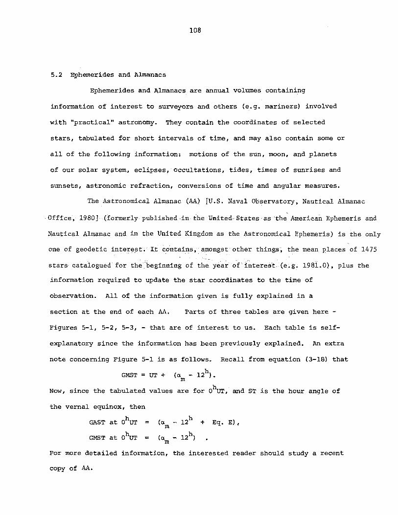
108
5.2 . E;phemexoides and Almanacs
Ephemerides and l\lmanacs are annual volumes containing
info:rmation of interest to surveyors and others (e.g. mariners) involved
with "practical" astronomy. They contain the coordinates of selected
stars, tabulated for short intervals of time, and may also contain some or
all of the following information: motions of the sun, moon, and planets
of our solar system, eclipses, occultations, tides, times of sunrises and
sunsets, astronomic refraction, conversions of time and angular measures.
The Astronomical Almanac (AA) [U.S. Naval Observatory, Nautical Almanac . ,
, Office, 1980]. ,(formerly,. published ,j;l1.thelJittted" States -as·'the· American Ephemeris and
Nautical Almanac and in 'the United Kingdom as the Astronomical Ephemeris) is the only
one of geodeticinte;-e~t:.· It'contai;lJs~amongst' other things~ the mean I?lac~s of 1475
s'tars- catalogued for the "beginning of theye'ar' of'irtteres"t, (e~ g~ 1981.0), plus the
information required to update the star coordinates to the time of
observation. All of the information given is fully explained in a
section at the end of each AA. Parts of three tables are given here -
Figures 5-1, 5-2, 5-3, - that are of interest to us. Each table is self-
explanatory since the info:rmationhas been previously explained. An extra
note concerning Figure 5-1 is as follows. Recall from equation (3-18) that
GMST = UT + (a - l2h). m
Now, since the tabulated values are for ohUT, and ST is the hour angle of
the vernal equinox, then
GAST at OhUT
GMST at OhUT
=
=
(a - l2h m
(a m
+ Eq. E),
For more detailed information, the interested reader should study a recent
copy of AA.

109
UNIVERSAL AND SIDEREAL TIMES. 1981
G. SIDEREAL TIME Equation of U.T. at OhG.M.S.T. Date Julian (G. H. A. of the Equinox) Equinoxes G.S.D. (Greenwich Transit of
OhU.T. Date Apparent Mean atOhU.T. OhG.S.T. the ~fean Equinox)
244 .11 III • I • 245 II m • Jan. 0 4604.5 6 38 17.1886 17.9594 -0.7708 1299.0 Jan. 0 17 1851.3829
1 4605.5 6 42 13.7431 14.5148 .7717 1300.0 1 17 1455.4734 2 4606.5 6 46 10.2993 11.0702 .7708 1301.0 2 17 1059.5639 3 4607.5 6 50 06.8575 07.6255 .7681 1302.0 3 17 07 03.6545 4 4608.5 6 54 03.4174 04.1809 .7635 1303.0 4 17 0307.7450
5 4609.5 6 57 59.9787 60.7363 -0.7576 1304.0 5 16 59 11.8356 6 4610.5 7 01 56.5407 57.2916 .7510 1305.0 6 16 55 15.9261 7 4611.5 7 05 53.1023 53.8470 .7447 1306.0 7 16 51 20.0166 8 4612.5 7 09 49.6626 50.4024 .7398 1307.0 8 16 47 24.1072 9 4613.5 7 13 46.2207· 46.9577 .7370 1308.0 9 16 4328.1977
/
10 4614.5 7 17 42.7763 43.5131 -0.7368 1309.0 10 16 39 32.2882 11 4615.5 7 21 39.3297 40.0685 .7387 1310.0 11 16 35 36.3788 12 4616.5 7 25 35.8817 36.6238 .7421 1311.0 12 16 31 40.4693 13 4617.5 7 29 32.4335 33.1792 .7457 1312.0 t3 16 27 44.5598 14 4618.5 7 33 28.9864 29.7346 .7481 1313.0 14 16 23 48.6504
15 4619.5 ·7 37 25.5415 26.2899 -0.7484 1314.0 IS 16 1.9 52.7409 16 4620.5 7 41 22.0994 22.8453 .7459 1315.0 16 16 15 56.8314 17 4621.5 7 45 18.6598 19.4006 .7409 1316.0 17 16 1200.9220 18 4622.5 7 49 15.2219 15.9560 .7341 1317.0 18 16 08 05.0125 19 4623.5 7 53 11.7843 12.5114 .7271 1318.0 19 16 04 09.1030
20 4624.5 7 57 08.3457 09.0667 -0.7210 1319.0 20 16 00 13.1936 21 4625.5 . 8 01 04.9050 05.6221 .7171 1320.0 21 15 56 17.2841 22 4626.5 8 05 01.4618 02.1775 .7157 1321.0 22 15 52 21.3746 23 4627.5 8 08 58.0160 58.7328 .7168 1322.0 23 IS 48 25.4652 24 4628.5 8 12 54.5682 55.2882 .7199 1323.0 24 IS ·44 29.5557
25 4629.5 8 16 51.1192 51.8436 -0.7243 1324.0 25 15 40 33.6462 26 4630.5 8 20 47.6698 48.3989 .7291 1325.0 26 15 3637.7368 27 4631.5 8 24 44.2208 44.9543 .7335 1326.0 27 15 3241.8273 28 4632.5 8 28 40.7728 41.5097 .7368 1327.0 28 15 2845.9178 29 4633.5 8 32 37.3264 38.0650 .7386 1328.0 29 15 2450.0084
30 4634.5 8 36 33.8818 34.6204 -0.7386 1329.0 30 15 2054.0989 31 4635.5 8 40 30.4389 31.1758 .7368 1330.0 31 15 1658.1894
Feb. I 4636.5 8 44 26.9975 27.7311 .7336 1331.0 Feb. I IS 1302.2800 2 4637.5 8 48 23.5571 24.2865 .7294 1332.0 2 15 09 06.3705
3 4638.5 8 52 20.1168 20.8418 .7251 1333.0 3 15 05 10.4610
4 4639.5 8 56 16.6755 17.3972 -0.7217 1334.0 4 15 01 14.5516 5 4640.5 9 00 J3.2323 13.9526 .7203 1335.0 .s 14 57 18.6421 6 4641.5 9 04 09.7865 10.5079 .7215 1336.0 6 14 53 22.7326 7 4642.5 9 08 06.3381 07.0633 .7252 1337.0 7 14 '4926.8232 8 4643.5 9 12'02.8879 03.6187 .7307 1338.0 8 14 45 30.9137
9 4644.5 9 15 59.4372 60.1740 -0.7369 1339.0 9 14 4135.004·2 10 4645.5 9 19 55.9872 56.7294 .7422 1340.0 10 14 37 39.0948 11 4646.5 9 23 52.5392 53.2848 .7455 1341.0 11 14 3343.1853 12 4647.5 9 27 49.0938 49.8401 .7463 1342.0 12 14 2947.2758
13 4648.5 9 31 45.6509 46.3955 .7445 1343.0 13 14 2551.3664
14 4649.5 9 35 42.2098 42.9509 -0.7411 1344.0 14 14 21 55.4569 15 4650.5 9 39 38.7693 39.5062 -0.7369 1345.0 15 14 17 59.5474
Figure 5-1 [AA, 1981]
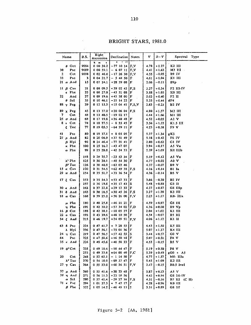
110
BRIGHT STARS, 1981.0
Name B.S. Right
Declination Notes V B-V Spectral Type Ascension h DI • 0 . ..
B Ocl 9OS4 000 38.2 -77 10 14 F,V 4.78 +1.27 K2 III 30 Psc 90S9 000 59.1 - 607 11 F,V 4.41 +1.63 M3 III 2 Cet 9098 002 46.0 -17 26 30 F,V 4.55 -0.05 B9 IV
33 Psc 3 004 21.7 -54850 F 4.61 +1.04 Kl III 21 a And IS 007 24.1 +28 59 08 F 2.06 -0.11 B9p
11 fJ Cas 21 008 09.3 +59 02 42 F.S 2.27 +0.34 F2 III-IV E Phe 25 o OS 27.0 -45 51 08 F 3.S8 +1.03 KO III
22 And 27 009 19.6 +45 58 00 F 5.03 +0.40 F2 II B Sci 35 o 10 46.1 -35 14 22 F 5.25 +0.44 dF4
88 y Peg 39 o 12 15.3 +15 04 41 F,S,V 2.83 -0.23 B21V
89 " Peg 45 o 13 37.0 +200604 F,S 4.80 +1.57 M2 III 7 Cet 48 o 13 40.5 -1902 17 4.44 +1.66 MI 111
2S fT And 68 o 17 19.8 +36 40 4S F 4.52 +0.05 A2 V 8 , Cet 74 o 18 27.5 - 8 55 45 F 3.S6 +1.22 Kl.S III
t Tuc 77 o 19 OS.3 -64 59 11 F 4.23 +0.58 F9 V
41 Psc 80 o 19 37.1 + 805 OS F 5.37 +1.34 gK3 27 p And 82 o 20 06.9 +37 51 49 F 5.18 +0.42 F6 IV
fJ Hyi 98 o 24 46.4 -77 21 41 F 2.80 +0.62 Gl IV Ie Phe 100 o 25 16.2 -43 47 07 3.94 +0.17 A5 Vn a Phe 99 025 20.S -4224 33 F 2.39 +1.09 KO IlIb
118 o 29 25.7 -23 53 34 F 5.19 +0.12 A5 Vn AI Phc 125 o 30 30.1 -48 54 30 F 4.77 +0.02 AO V fJlTuc 126 030 40.8 -63 03 46 4.37 -0.07 B9 V
IS Ie Cas 130 o 31 54.5 +62 49 38 F,S 4.16 +0.14 Bl la 29 'II' And 154 o 35 51.7 +33 3654 F 4.36 -0.14 BS V
17 t Cas 153 o 35 54.3 +53 47 33 F 3.66 -0.20 B2 IV 157 o 36 19.8 +35 17 43 S 5.48 +0.88 G3 11
30 E And 163 037 32.8 +29 12 32 F 4.37 +0.87 G8 IlIp 31 8 And 165 o 38 18.5 +3045 26 F,S 3.27 +1.28 K3 III 18 a Cas 168 o 39 25.2 +562600 F,V 2.23 +1.17 KO- IlIa
". Phe 180 040 25.8 -46 11 21 F 4.59 +0.97 G8 III '1 Phc 191 042 30.2 -57 34 02 F,D 4.36 +0.00 B9 Vp
16 fJ Cel 188 042 38.1 -1805 27 F 2.04 +1.02 Kl JJl 22 0 Cas 193 043 39.6 +48 10 50 F 4.54 -0.07 B5 III 34 , And 21S 046 19.7 +24 09 51 F,V 4.06 +1.12 KIll
63 8 Psc 224 o 47 41.7 + 728 55 F 4.43 +1.50 K5 III A Hyi 236 o 47 56.1 -75 01 36 F 5.07 +1.37 K4 III
24 .., Cas 219 047 56.5 +57 42 55 S 3.44 +0.57 GO V 64 Psc 225 047 58.6 +16 50 18 F 5.07 +0.51 F8 V 35 " And 226 04845.6 +40 58 33 F 4.53 -0.15 B5 V
19 4I"Cct 235 049 10.4 -104447 F 5.I9 +0.50 F8 V 233 049 33.6 +64 OS 40 F,C 5.39 +0.49 gGO + A5
20 Cct 248 o 52 02.1 - I 14 50 F 4.77 +1.57 MO- Ula A"Tuc 270 o 54 18.0 -69 37 47 F 5.45 +1.09 K2 III
27 y Cas 264 055 33.0 +6036 51 F,V 2.47 -0.15 BO.S IYel
37 ". And 269 o 55 41.6 +38 23 48 F 3.87 +0.13 A5 V 38 .., And 271 o 56 11.3 +23 18 56 4.42 +0.94 G8 Ill-IV
a Sci 280 o 57 41.4 -29 27 36 F.S 4.31 -0.16 B7 III (C II) 71 E Psc 294 I 01 57.3 + 7 47 17 F 4.28 +0.96 KO III
fJ Phe 322 I OS 14.2 -46 49 13 2 3.31 +0.89 G8 III
Figure 5-2 [AA, 1981]
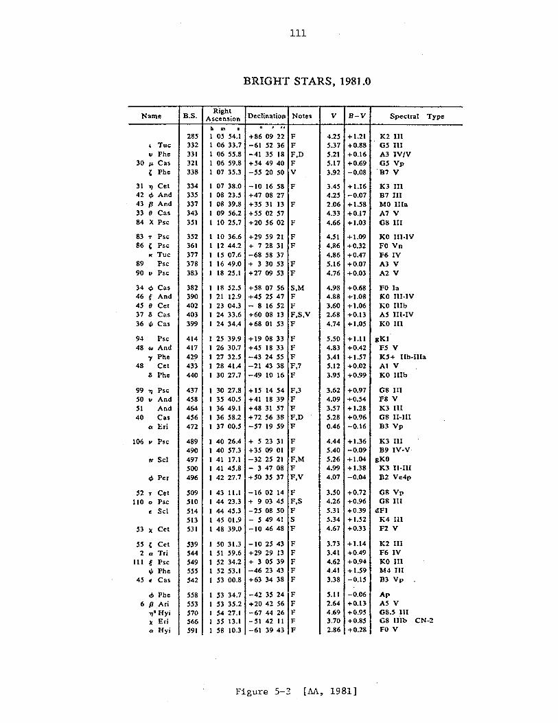
111
BRIGHT STARS, 1981.0
Nama B.S. Right
Declination Notes V B-V Spectral Type Ascension II In I . ,
" 285 1 05 54.1 +8609 22 F 4.25 +1.21 K2I11 , Tuc 332 1 06 33.7 -61 52 36 F 5.37 +0.88 05 III
II Phe 331 1 06 55.8 -41 35 18 F,D 5.21 +0.16 -A3 IV/V 30 p. Cas 321 1 0659.8 +54 49 40 F 5.17 +0.69 05 Vp
, Phe 338 1 07 35.3 -55 20 50 V 3.92 -0.08 'B7 V
31 'IJ Cet 334 I 07 38.0 -10 1658 F 3.45 +1.16 Kl III 42 <I> And 335 1 08 23.5 +47 08 27 4.25 -0.07 87 III 43 fJ And 337 1 08 39.8 +35 31 13 F 2.06 +1.58 MO lila 33 8 Cas 343 I 09 56.2 +55 02 57 4.33 +0.17 A7 V 84 X Psc: 351 1 10 25.7 +205602 F 4.66 +1.03 08 III
83 T Psc: 352 1 10 36.6 +295921 F 4.51 +1.09 KO III·IV 86 , Psc: 361 1 1244.2 + 728 31 F 4.86 +0.32 FO Vo
Ie Tuc: 377 I 15 07.6 -68 58 37 4.86 +0.47 F6 IV 89 Psc: 378 1 1649.0 + 3 3053 F 5.16 +0.07 A3 V 90 " Psc: 383 1 18 25.1 +270953 F 4.76 +0.03 A2 V
34 <I> Cas 382 1 18 52.5 +5807 56 S,M 4.98 +0.68 FO Ia 46 ( And 390 1 21 12.9 +45 25 47 F 4.88 +1.08 KO III·IV 45 8 Cet 402 1 23 04.3 - 8 1652 F 3.60 +1.06 KO IlIb 37 3 Cas 403 1 24 33.6 +6008 13 F.S,V 2.68 +0.13 AS III·IV 36 til Cas 399 1 24 34.4 +68 01 53 F 4.74 +1.05 KO II1
94 Psc: 414 I 25 39.9 +1908 33 F 5.50 +1.11 SKI 48 Co> And 417 1 26 30.7 +45 18 33 F 4.83 +0.42 FS V
'Y Phe 429 I 27 32.5 -43 24 55 F 3.41 +1.57 K5+ lIb-lIla 48 Cet 433 I 28 41.4 -21 43 38 F.7 5.12 +0.02 AI V
3 Phe 440 1 30 27.7 -49 10 16 F 3.95 +0.99 KO lIIb
99 'I Psc: 437 1 30 27.8 +15 1454 F,3 3.62 +0.97 G8 111 50 " And 458 1 35 40.5 +41 18 39 F 4.09 +0.54 FS V 51 And 464 1 36 49.1 +48 31 57 F 3.57 +1.28 K3 III 40 Cas 456 1 36 58.2 +72 56 38 F,D 5.28 +0.96 08 It·III
a Eri 472 1 37 00.5 -57 19 59 F 0.46 -0.16 83 Vp
106 I' Psc: 489 1 40 26.4 + 5 23 31 F 4.44 +1.36 K3 III 490 1 40 57.3 +35 09 01 F 5.40 -0.09 B9 IV·V
f'( Scl 497 1 41 17.1 -32 25 21 F,M 5.26 +1.04 gKO 500 1 41 45.8 - 347 08 F 4.99 +1.38 K3 II·III
<I> Per 496 1 42 27.7 +5035 37 F,V 4.07 -0.04 B2 Ve4p
52 T Cet 509 1 43 11.1 -1602 14 F 3.50 +0.72 G8 Vp llO 0 Psc 510 1 44 23.3 + 903 45 F,S 4.26 +0.96 G8 III
E ScI 514 1 44 45.3 -25 08 50 F 5.31 +0.39 dFI 513 1 45 01.9 - 54941 S 5.34 +1.52 K4 III
S3 X Cet 531 I 48 39.0 -104648 F 4.67 +0.33 FlV
55 , Cet 539 I 50 31.3 -102543 F 3.73 +1.14 K2 111 2 a Tri 544 I 51 59.6 +2929 13 F 3.41 +0.49 F6 IV
III ( Psc: 549 1 52 34.2 + 3 05 39 F 4.62 +0.94 KO J1l til Phe 555 1 52 53.1 -4623 43 F 4.41 +1.S9 M4III
45 « Cas 542 1 53 00.8 +63 34 38 F 3.38 -0.15 B3 Vp
<I>,Phe 558 1 53 34.7 -42 35 24 F S.1l -0.06 Ap 6 IJ ,Ari 553 I 53 35.2 +2042 56 F 2.64 +0.13 A5 V
1)' Hyi 570 I 54 27.1 -67 44 26 F 4.69 +0.95 G8.S 1lI
)( Eri 566 I 5S 13.1 -SI 42 II F 3.70 +0.85 G8 nIb CN·2 o Hyi S91 1 58 10.3 -61 3943 F 2.86 +0.28 FO V
Figure 5-3 [AA, 1981}
112
The Star Almanac for Land Surveyor§ (SALS) rH.M. Nautical
Almanac Office, 1_980], published annually, is expressly designed to meet
the surveyor's requirements in astronomy. The main tables included are:
(i) the Sun, in which the right ascension, declination, and
equation of time are tabulated for 6-hourly intervals (see
explanations below regarding Figure 5-4),
(ji) the Stars, in which the apparent right ascension and
declination of 685 stars are given for the beginning of each
h ~onth (e.g. 0 UT, March 1, 1981),
(iii) Northern and Southern Circumpolar Stars (five of each), are
listed separately, their apparent right ascensions and de-
clinations being given at lO-day intervals for the year,
(iv) the Pole Star Table, a special table for Polaris (n Ursae
Minoris) for use in specific math models for latitude and
azimuth determinations.
Also included in SALS are several supplementary tables, some of
which are companions to those noted above (for interpolation purposes).
Examples of three SALS tables are given in Figures 5-4, 5-5, and 5-6.
Most of the information given has been explained previously, and the tables
are self explanatory. Regarding the terms R and E in Figure 5-4, one
should note that
R=
E =
h (n - 12 + Eq.E) =
m h
Eq.T. - 12 •
GAST at ohUT,
The reader is cautioned that SALS is not suitable for use where
first-order standards mus-t be met.<AA < may be used, but common practice
is to use one of the fundamental catalogues and compute the updated star
coordinates via procedures outlined in Chapter 6.
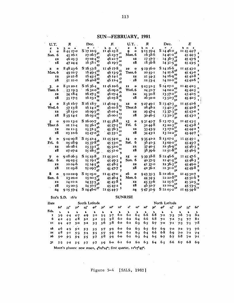
U.T. d " 1 0
Sun. 6 12 18
2 0
Mon. 6 12 18
3. 0 Tues. 6
12 18
... 0 Wed. 6
12 18
5 0 Thur.6
:12
18
6 0 Fri. 6
12 18
7 0 Sat. 6
12 18
8 0
Sun. 6 12 18 24
113
SUN-FEBRUARY, 1981
U.T •. d " 9 0
Mon. 6 12 ' 18
10 0
Tues. 6 :12
. 18
II 0 Wed, 6
:12
:18
1:Z 0
Thur,6 12 18
IJ 0 Fri. 6
12 18
14 0 Sat. 6
12 18
IS 0 Sun. 6
12 18
16 0
Mon. 6 12 i8 24
R
9 1956,0 20 55'1 21 54'3 2253'4
9 2352 '5 2451'7 2550,8 26 5°'°
9 2749.1 28 48'2
2947'4 3°46'5
,931 45'7 32 44.8 3343'9 3443.1
93542 •2 36 41 '3 3740'5 38 39.6
93938.8 4°37'9 41 37'0 42 36.2
94335'3 44 34'5 4533.6 46 32 '7
94731'9
Dec. E .. m •
II 4544'7 ' 4544'3 : 4543'9 4 4543'5 3
II 45 43'2 4543.0 2
4542 •8 2
4542•6 2 I
I 1 4542'S 4542 '5 0
4542'5 0
4542'5 0 I
II 45 42 ,6 4542,8 2
4543'0 2
4543.2 2 3
II 4543'5 4543,8 3 4544'2 4
5 4544'7 4 :
II 4545.1 6
4545'7 6 4546'3 6 4546'9 7
II 45 47·6 4548'3 7
45 49'0 ~ 4549.8
9 II 45 50'7
4551•6 9 4552'5 9 4553'S 10
114554.611
Sun"s S.D, 16=2 SUNRISE
Date
Feb. 60- 5S·
" " :I 3'9 4'4 6 4'2 4'5
4'4 4-7 II
South Latitude North Latitude ~ ~ ~ ~ ~ ~ ~ ~ ~ ~ ¢ ~ ~ ~ W
II .. II " II II • 110 II • " II • II II 4'7 4'9 5,2 5'5 5'7 6·0 6,2 6'4 6·6 6·8 7'2 7'3 7·6 7'9 8,% 4.8 5.1 5'% 5'5 5.8 6·0 6·% 6'4 6,6 6·8 7·1 7.2 7'5 7'7 8'1 5,0 5,2 S'J 5.6 5,8 6'0 6'2 6'J 6'5 6'7 7'0 7-I' 7'3 7'5 7,8
16 4.6 4'9 5-1 5'3 5'5 5'7 5'9 6'0 6,2 21 4.8 5'1 5'3 5'4 5'5 5'7 5'9 6·0 6'2 :z6 5'0 5-3 5'4 5'5 5'7 5.8 5'9 6'0 6,2
6'3 6'5 6'7 6'9 6'3 6'4 6·6 6·8 6'3 6'4 6'5 6'7
7'0 7,2 7'3 7·6 6'9 7'0 7·2 7'4 6'7 6·8 7·0 7,1
31 5'3 5'4 5'5 5'7 5'7 5'9 6'0 6,1 6·% 6,2 6'3 6'4 6'5 6·6 6'7 6-8 6'9
Figure 5-4 [SALS, 1981J
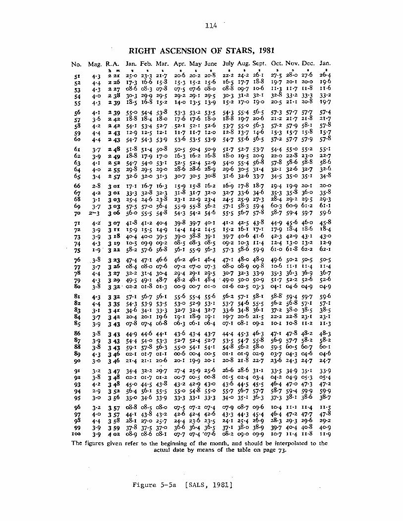
114
RIGHT ASCENSION OF STARS, 1981
No. Mag. R.A. Jan. Feb. Mar. Apr. May June July Aug. Sept. Oct. Nov. Dec. Jan. II m • • •
5' 4-3 221 25-0 23-3 21'7 52 4'4 2. 26 17'3 16·6 15.8 53 4-3 22.7 oS-6 oS'3 07.8 54 4-0 238 30-3 29'9 29'5 55 4'3 2. 39 18'5 16·8 15.2
56 4'1 2. 39 55'0 54'4 53.8 57 3.6 2. 42 IS·8 IS'4 18'0 58 4.2 2. 42 54.1 53'4 52'7 S9 4'4 2. 43 12'9 12'5 12'1
60 4'4 243 54'7 54'3 53'9
61 62 63 64 65
51'S 51'4 50·8 IS,S 17'9 17'0 54-7 54'0 53.1 29.8 29'5 29.0
66 6'] 68
2·8 301 32 •6 32 '° 31'3 17·1 16'7 16'3 33'3 32.8 32'3 25'4 24·6 23.8 57'5 57'0 56'4 56-0 55'5 54.8
69 70
71
72
73 74 75
76 77 78 79 80
4'2 3'9 3-9 4'3 1'9 '
3.8 3'7 4'4 4'3 3-8
81 4'3 82 . 4'4 83 3.1
84 3'7 85 3'9
86 S, 88 B9 90
3 01 3 0 3 3 0 3 3 06
30'] 41.8 'P'2 40'4 3 u: 15'9 15-5 14'9 3 18 40'4 4°-0 39'5 3 19 10'5 09-9 09'2 3 Z% 5S-2 57·6 56-8
3 23 47'4 47-1 46-6 3 26 oS-4 oS·o 07·6 3 2 7 32'2 31 '4 3004 3 29 49'5 49-1 48'7 332' 02·2 01·8 01'3
332. 57'1 56'7 56.1 33S 54'3 53'9 53'5 341 34.6 34'1 33'3 342 20'4 20'1 19.6 3 43 07·8 07-4 06·8
343 343 343 346 346
44'9 44·6 44. 1
54'4 54'0 53-3 59.1 57.8 56'3 02·1 01'7 01·1 21'4 21·1 20·6
91 3'2 347 34'4 32'2 29'7 9Z 3·8 348 02-1 01'7 01·2 93 4'2 34f8 45-0 44'5 43.8 94 2'9 352 56'4 56.1 55-5 95 3'0 3 56 35-0 34.6 33-9
¢ 3'2 3 57 oS·8 oS'5 oS·o 97 4'0 357 44.1 43.8 43.2 C)8 4'4 3 58 28,1 27'0 25'7 99 3'9 3 59 37.8 37' 5 37'0
100 3-9 402 oS-9 oS·6 oS'I
• • • 20·6 20·2 20·8 15'3 15'2 15.6 07'5 07·6 oS-o 29.2 29' 1 29-5 14'0 13'5 13'9
53'3 53'2 53-5 17-6 17·6 IS,O
.52'1 52.1 52.6 II'7 II'7 12-0 53.6 53-5 53-9
S0· 5 50'4 50'9 16'3 16,2 16·S 52 '5 52 '4 52 '9 28·6 2S·6 28'9 30'7 30 -5 30 ;8
15'9 15.8 16'2 31.8 31'7 32'° 23.1 22'9 ~3'4
55'9 55.8 56'2 54'3 54.2 54.6
• • s 22·2 24.2 26,1 16'5 17'7 18·8 oS·8 09'7 10·6 30'3 31.2 32.1 15,'2 17.0 19'0
54'3 55'4 56'5 18·8 19-7 20·6 53'7 55'0 56'3 12·8 13'7 14·6 54'7 55.6 56'5
51'7 52'7 53'7 18'0 19'5 20'9 54'0 55'4 56.8 29.6 30'5 31'4 31.6 32.6 33'7
16:9 17.8 18'7 32'7 33.6 34.6 24'5 25'9· 27'3 57'1 58'3 59-4 55'5 56'7 57.8
39.8 39'7 40'1 41-2 42'5 43.8 14'4 14'2 14'5 15'2 16,1 17.1 39'0 38.8 39.1 39-7 40·6 41.6 oS'5 oS'3 oS'5 09'2 10'3 II'4 56.1 55'9 56'3 ,57'3 58.6 59'9
46'2 46.1 46'4 47'1 48.0 48'9 07'2 07'0 07'3 oS·o oS'9 09.8 29'4 29'1 29'5 30'7 32'3 33'9 48.2 48.1 48'4 . 49'0 50·0 50'9 00'9 00'7 01'0 01·6 02'5 03'3
55.6 55'4 55.6 56'2 57.1 58'1 53.0 52'9 53.1 53'7 54.6 55'5 32'7 32'4 32'7 33.6 34.8 36. I 19.1 18'9 19'1 19'7 20·6 21'5 06'3 06,1 06'4 07'1 oS'l 09'2
43.6 43'4 43'7 44'4 45'3 46'3 52'7 52'4 52'7 53'5 54'7 55.8 55'0 54.1 54'1 54.8 56'2 58,° 00·6 00'4 00'5 01'1 01'9 02'9 20·1 19'9 20'1 20·8 21·8 22'7
27'4 25'9 25.6 26·6 28-6 31.1
00-7 00'5 00·8 01'5 02'4 03'4 43'2 42'9 43'0 43·6 44-5 45'5 55.0 54.8 55'0 55'7 56'7 57'7 33'3 33'1 33'3 34'0 35.1 36'3
07'5 07-2 07'4 07'9 oS-7 09.6 42.6 42'4 42.6 43'3 44'3 45'4 24'4 23·6 23'5 24- 1 25'4 26'9 36.6 36'4 36'5 37·1 38,° 38-9 07'7 07'4 -07·6 oS'2 09-0 09'9
I I I
27-5 28'0 27·6 19'7 20'1 20·0 11'3 II-7 u·8 32.8 33'2 33'3 20'5 21'1 20·8
57'3 57'7 57'7 21·2 21'7 21·8 57·2 57'9 58. I 15'3 15'7 15.8 57-2 57'7 57'9
54'4 55-0 55.2 22·0 22·8 23'0 57-8 58.6 58.8 32'1 32.6 32'7 34'S 35'0 35.1
19'4 19'9 20·1 35'3 35.8 36'0 28'4 29'2 29'5 60'3 60'9 61'2 58'7 59'4 59'7
44-9 45·6 46•0
17'9 18'4 18·6 42-3 42'9 43'1 12'4 t 3.0 13-2 61'0 61·8 62·2
49.6 50·2 50-5 10·6 11'1 II'4 35'3 36'3 36'9 51'7 52'2 52.6 04'1 04·6 04'9
58.8 59'4 59'7 56.2 56.8 57- I
37'2 38'0 38'5 22'2 22·8 23.1 10-1 10·8 II·2
47·1 47·8 48'2 56-9 57'7 58.2 59' 5 60'5 60-7 03'7 04'3 °4.6 23.6 24'3 24-7
33'5 34'9 35.1 04.2 04'9 05-3 46-4 47'0 47'3 58-7 59'4 59'9 37'3 38'1 38.6
10'4 II'I II-4 46'4 47'2 47-7 28· 3 29' 3 29.6 39'7 4004 40.8 10'7 1I'4 II·8
• 26'4 19.6 II·6 33.2
'19'7
57'4 21'7 57.8 15'7 57-8
55- I
22'7 58.6 32•6. 34.8
20·0 35.8 29'3 61·1 59.6
45.8 18'4 43'° 12'9 62-1
50 '5 II'4 36'7 52 •6 04'9
59.6 57'1 38'5 23'1 II'3
48'3 58'2 60,1 04.6 24'7
33'9 °5'4 47'2 59'9 38'7
II'S 47.8 29.2 4°'9 11'9
The figures given refer to the beginning of the month. and should be interpolated to the actual date by means of the table on page 73-
Figure 5-5a [SALS, 1981]
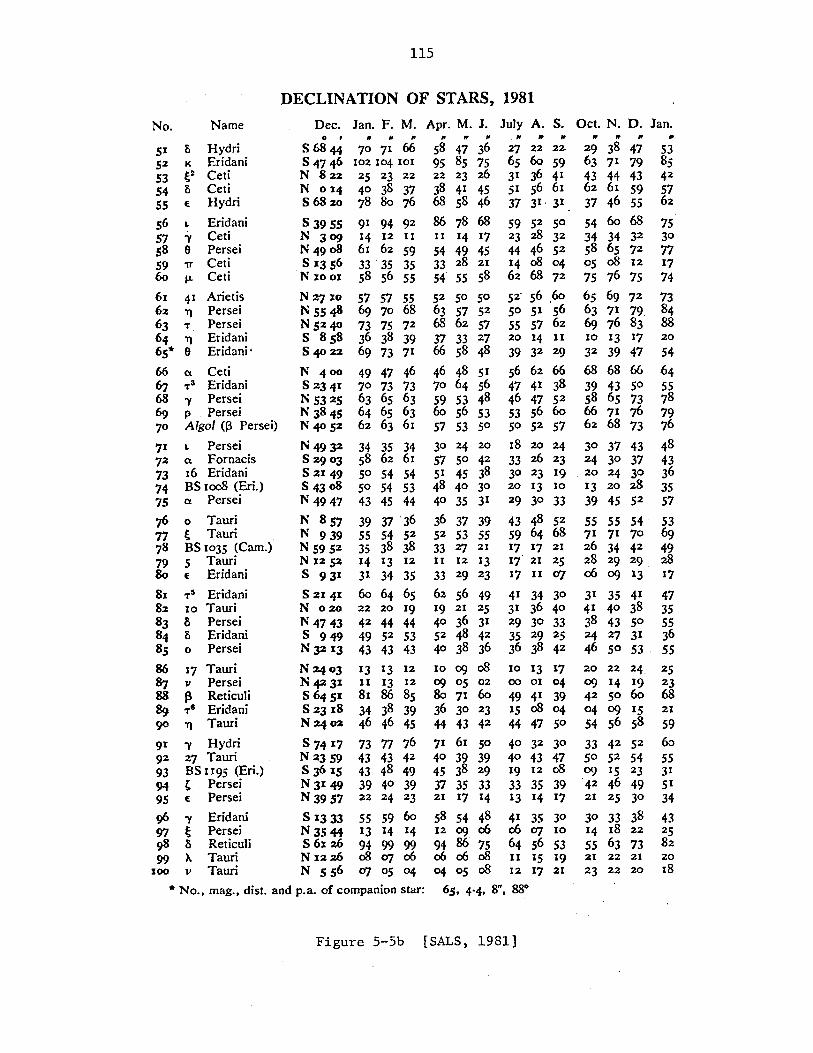
115
DECLINATION OF STARS, 1981
No. Name Dec. Jan. F. M. Apr. M. J. July A. S. Oct. N. D. Jan. G • " II " II II II ," " " II " " " 51 8 Hydri S6844 70 71 66 58 47 36 27 22 22 29 38 47 53
52 K Eridani S4746 102104101 95 85 75 65 60 59 63 71 79 85 S3 ~2 Ceti N 822 25 23 22 22 23 26 31 36 41 43 44 43 42 S4 8 Ceti N 014 40 38 37 38 41 45 51 56 61 62 61 S9 57 5S E Hydri S6820 78 80 76 68 58 46 37 31 31 37 46 5S 62
S6 L Eridani S 39 5S 91 94 92 86 78 68 59 52 50 54 60 68 75 57 'Y Ceti N 309 14 12 II II 14 17 23 28 32 34 34 32 30 58 e Persei N49 08 61 62 59 54 49 45 44 46 52 S8 65 72 77 59 'IT Ceti ,S 1356 33 3S 3S 33 28 21 14 08 04 05 08 12 17 60 j.l. Ceti N 1001 58 56 55 54' 55 58 62 68 72 75 76 75 74 61 41 Arietis N2'] 10 57 57 55 52 50 50 52' 56 .60 65 69 72 73 6% TJ Persei N SS..s 69 70 68 63 57 52 50 51 56 63 71 79, 84 63 T Persei N 5%40 73 75 72 68 62 57 55 57 6% 69 76 83 88 64 TJ Eridani S 858 36 38 39 37 33 27 20 14 II 10 13 17 20 65· e Eridani' S 40 2.Z 69 73 71 66 58 48 39 32 29 32 39 47 54 66 (It Ceti N4 00 49 47 46 46 48 51 56 62 66 68 68 66 64 67 T3 Eridani S2341: 70 73 73 70 64 56 47 41 38 39 43 50 55 68 'Y Persei N 5325 63 65 63 59 53 48 46 47 5% 58 65 73 78 69 p Persei N 3845 64 65 63 60 56 53 53 56 60 66 71 76 79 70 Algol (13 Persei) N40S2 62 63 61 57 53 50 50 52 57 62 68 73 76
'11 L Persei N4932 34 35 34 30 24 20 18 20 24 30 37 43 48 '12 (It Fornacis S29 03 58 62 61 57 SO 42 33 26 23 24 30 37 43 '13 16 Eridani S21: 49 50 54 54 51 45 38 30 23 19 ,20 24 30 36 74 BS 1008 (Eri.) S43 08 50 54 53 48 40 30 20 13 10 13 20 28 35 7S (It Persei N4947 43 45 44 40 35 31 29 30 33 39 45 52 57
76 0 Tauri N 857 39 37'36 36 37 39 43 48 52 55 55 54 ' 53 77 ~ Tauri N 939 55 54 52 52 53 55 59 64 68 71 71 70 69 78 BS 1035 (Cam.) N 595% 35 38 38 33 27 21 17 17 21 26 34 42 49 79 5 Tauri N 12,52 14 13 12 II 12 13 17 21 25 28 29 29, 28 80 E Eridani S 931: 31 34 35 33 29 23 17 II 07 06 09 13 17 81 Til Eridani S 21 41 60 64 65 62 56 49 41 34 30 31 35 41 47 82 10 Tauri N020 22 20 19 19 21 25 31 36 40 41 40 38 35 83 & Persei N4743 42 44 44 40 36 31 29 30 33 38 43 50 55 84 & Eridani S949 49 52 53 52 48 42 35 29 %5 24 27 31 36 85 0 Persei N 32 x3 43 43 43 40 38 36 36 38 42 46 50 53 ' 55 86 17 Tauri N24 03 13 13 12 10 (1)08 10 13 17 20 22 24, 25 S, v Persei N 4231 II 13 12 (1) 05 02 00 01 04 09 14 19 23 88 13 Reticuli S645X SI 86 85 80 71 60 49 41 39 42 50 60 68 89 TI Eridani S23 x8 34 38 39 36 30 23 15 08 04 04 09 15 21 90 TJ Tauri N24 02 46 46 45 44 43 42 44 47 50 54 56 58 59
91 'Y Hydn S 7417 73 77 76 71 61 50 40 32 30 33 42 52 60 92 27 Tauri N 2359 43 43 42 40 39 39 40 43 47 50 52 54 55 93 BS 1195 (En.) S J6 IS 43 48 49 45 38 29 19 12 08 ,09 IS 23 31
94 t Persei N 31 49 39 40 39 37 3S 33 33 3S 39 42 46 49 51 95 E Persei N3957 22 24 23 21 17 14 13 14 17 21 25 30 34
96 'Y Eridani S x333 55 59 60 58 54 48 41 35 30 30 33 38 43 97 E Persei N3S44 13 14 14 12 (1) 06 06C1] 10 14 IS 22 25 98' & Reticuli S6126 94 99 99 94 86 75 64 56 53 55 63 73 82 99 ). Tauri N x226 08 C1] 06 060608 II 15 19 21 22 21 20
100 V Tauri N 5S6 C1] 05 04 04 05 08 12 17 21 23 22 20 18
• No., mag., dist. and p.a. of companion star: 65. 4'4. 8". 880
Figure 5-5b [SALS, 1981]
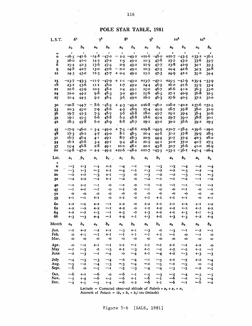
L.S.T.
m o 3 6 9
12
IS 18 21
24 27
30
33 J6 39 42
45 ',.s 51 54 57 60
Lat. o
o 10
20
30
40 45 50 $5 60 62 64 66
Month
Jan. Feb. Mar.
Apr. May June
JuJy Aug. Sept.
Oct. Nov. Dec.
, , -26'5 -41,6
26'0 42'0 25'4 42 '3 24,8 42'7 24'3 43'0
-23'7 -43'3 23'2 43.6 22,6 43'9 22-0 44,2 21'4 44'5
-20·8 -44'7 20'3 45'0 19'7 45'3 19. 1 45'S 18'5 45.8
-17'9 -46,° 17'3 46.2 16'7 46'4 16'1 46.6 15'4 46.8
-14.8 -47'0
-'3 -'3 -·2
-·2
,-·1
-·1 ·0
+·1 +,2 +·2 +·2 +'3
B2
-·2
·0
·0
·0 -·1 -'2
-'4 -'5 -·6 -·6 -'5 -'4
'0
-'1
-'1 -·2
-'2
-'3
-·2
-'3 -'3
-'3 -'2
'0
+'2 +'4 +'5
116
POLE STAR TABLE, 1981
, -14.8 -47'0
14'2 47.2 13·6 47'4 13.0 47·6 12'3 47'7
-I1'7 -47'9 II·I 48'0 10'5 48'2 9,8 48'3 9'2 48'4
- 8·6 -48'5 7'9 48,6 7'3 48'7 6·6 48.8 6,0 48'9
, . - 2·2
1'5
°'9 - 0·2
+ 0'4
-49'2 49'2 49'2 49.2
49.2
+ 1·1 -49'2 1'7 49'2 2'4 49.1 3'0 49.1
3.6 49'0
+ 4'3 -49'0 4'9 48'9 5.6 48.8 6'2 48.8 6·8 48'7
- 5'4 4'7 4.1
-49'0 ,+ 7'S -48.6 49'0 8,1 48'5
3'4 2·8
- 2·2
-'4 -'3 -'3 -·2
-·1 -·1
·0
+·1
+'2 +'2 +'3 +'4
-·2 . -·1
·0
·0 -·1
-'3 -'4 -'5 -·6 -·6 -'5
49'1 8'7 48'3 49'1 9'4 48.2
49'1 10·0 48.1 -49'2 +10·6 -48,°
·0
'0
·0 '0
-'1 -'1 -·1 -·1
'0
-·1
-'3 -'4
-'4 -'3 -·1
'0
+'2 +'4
-'4 -'4 -'3 -·2
-·1
-'1 ·0
+·1
+'2 +·2 +'3 +'4
-'3 -·1
·0
'0
-·2
-'3 -'5
-·6 -·6 -·6
-·1
-'1 '0
'0
·0 ·0 ·0
'0 '0 '0
+·1
b2
+-1 +·1
·0
-·1
-'3 -'4
-'4 -'4 -'3 --I
+'1 +·2
Bo , .
+10·6 -48,° II'3 47·8 u'9 47'7 12'5 47'5 13'1 47'3
+13'7 -47,1 14'4 46'9 15'0 46'7 ,15.6 46'5 16'2 46'3
+16·8 -46'1 17'4 45'9 18'0 45'7 18·6 45'4 19'2 45'2
+19.8 -44'9 20'4 44·6 20'9 44'4 21'5 44.1 22·1 43.8
+22-7 -43'5
-'4 -'3 -'3 -'2
-'3 -'2 -·2 -'1
-·1 -·1 -·1 ,0
·0 '0
+·1 +'1
+-2 +'1 +'2 +'2 +'3, +'2 +'3 +'2
B2 b2
-'3 '0
-·1 +·1 ,0 '0
+·1 -'1
+·1 -'2
+·1 -'4
-·1 '-'5 -·2 -'5 -'4 -'4
-'5 -'3 -·6 -·1
-·6 +-1
Jd'
+22'7 -43'5 23'2 43.2
23.8 42 '9 24'4 42.6 24'9 42 '2
+25'5 -41'9 26'0 41.6 26·6 41'2 2']-1 40'9 2'].6 40 -5
+28-2 -40,2 28'7 39.8 29'2 39'4 29'7 39'0 30'2 38.6
+3°-7 -38'2
31'2 37·8 31-7 37'4 32 •2 37-0
32'7 36.6 +33'2 -36'1
-'3 -·2
-·2
-·1
-I
oQ
+·1
+.J +2
. +-2 +'3
B2
-'3 -·1
-0
+·1 +,2, +'2 +.J -·1
-'3
-'5 -.6 --6
-'4 -'3 -'3 -'2
-'1 -·1
·0 +.J
+'2 +'2 +'3 +'3
hI -'1
'0 ·0
-.J
-'2
-'3
-'5 -'S -·S
-'4 -·2
-·1
Latitude = Corrected observed altitude of Polaris + a. + a, + 82
Azimuth of Polaris = (bo + bl + b2l sec (latitude)
Figure 5-6 [SALS, 1981]
, , +33'2 -36'1
33.6 35'7 34'1 35'3 34'5 ,34.8 35'0 34'4
+35'4 -33'9 35'9 33'4 36'3 33'° 36•8 32'5 37'2 32•0
+37·6 -31'5 38•0 31'0
38'4 3°·6 38.8 3°,1 39'2 29'5
+39.6 -29-0
39'9 28'5 40'3 28,0 40'7 27-S 41 '° 26'9
+41 '4 -26'4
-'2 -'2 -·1 -·1
-·1 ·0 ,0
,0
-·2 -.J
'0
+,2 +·2 +'3
+'2 ·0
-·2
-'3 --S -·6
-'4 -'4 -'3 -'2
-'1 -·1
'0
+·1
+'2 +'2 +'3 +'4
bl
--I
-0
'0
·0 -·1
-'3
-'4 -'S -'S
-·s -'4 -'2
6. VARIATIONS IN CELESTIAL COORDINATES
The mathematical models for the determination of astronomic
latitude, longitude, and azimuth require the use of a celestial bodies
apparent (true) coordinates for the epoch of observation. The coordinates
(a,S) of the stars and the sun (the most often observed celestial bodies
for surveying purposes) are given in star catalogues, ephemerides, and
almanacs for certain predicted epochs that do not (except in exceptional
circumstances) coincide with the epoch of observation. To fulfill the
requirements stated previously, the coordinates (a,~) must be updated. As
was indicated in Chapter 5, the updating procedure has been made very
simple for users of annual publications such as ,".,,~.j SALS, and APFS. The
question is, how are the coordinates in the annual publications derived,
and how should one proceed when using one of the fundamental star
catalogues (eg. FK4). The aim of this chapter is to answer this
question.
In previous discussions in these notes, coordinates in the Right
Ascension system have been considered constant with respect to time, and
in the Hour Angle and Horizon systems, changes occurred only as a result
of earth rotation. In this chapter, we consider the following motions in
the context of the Right Ascension system:
(i) precession and nutation: motions of the coordinate system
relative to the stars;
(ii) proper motion: relative motion of the stars with respect to
each other;
(iii) refraction, aberation, parallax: apparent displacement of
stars due to physical phenomena;
117
118
(iv) polar motion: motion of the coordinate system with respect to the
solid earth.
Except for polar motion, the above factors are discussed in terms
of their effects on a and 0 of a celestial body. This leads to variations
in the Right Ascension coordinate system. The definition of the variations
are given below and Figure 6-1 outlines their interrelationships.
(i) Mean Place: heliocentric, referred to some specified mean
equator and equinox.
(ii) True Place: heliocentric, referred to the true equator and
equinox of date when the celestial body is actually observed.
(iii) Apparent Place: geocentric, referred to the true equator and
equinox of date when the celestial body is actually observed.
(iv) Observed Place: topocentric, as determined by means of direct
readings on some instrument corrected for systematic
instrumental errors (e.g. dislevellment, collimation).
The definitions are amplified in context in the following sections.
6.1 Precession, Nutation, and Proper Motion
The resultant of the attractive forces of the sun, moon, and
other planets on our non-symmetrical, non-homogeneous earth, causes a
moment which tries to rotate the equatorial plane into the ecliptic
plane. We view this as the motion, of the earth's axis of rotation about
the ecliptic pole. This motion is referred to as precession. The
predominant effect of luni-solar precession is a westerly motion of the
equinox along the equator of 50~3 per year. The period of the motion is
approximately 26000 years, and its amplitude (obliquity of the ecliptic)
is approximately 23~5. Superimposed on this planetary precession, which
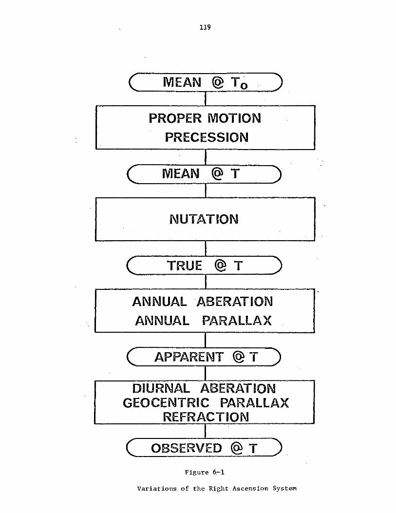
119
MEAN @ To . ) I
PROPER MOTION
PRECESSION
I ( MEAN @ T
I
NUTATION
I TRUE @ T
I ANNUAL 'ABERATION
ANNUAL PARALLAX
I APPARENT @ T
I DIURNAL ABERATION
GEOCENTRIC PARALLAX REFRACTION
J OBSERVED @ T
Figure 6,-1
Variations of the Right Ascension Syste~
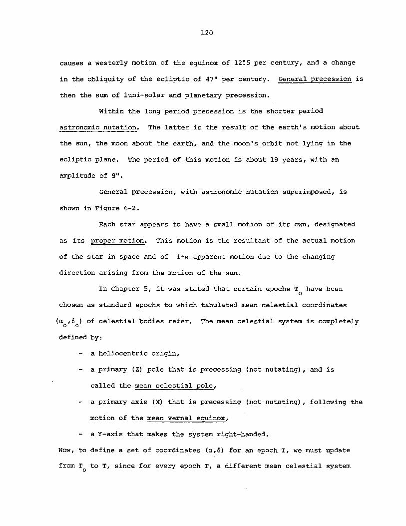
120
causes a westerly motion of the equinox of l2~5 per century, and a change
in the obliquity of the ecliptic of 47" per century. General precession is
then the sum of luni-so1ar and planetary precession.
Within the long period precession is the shorter period
astronomic nutation. The latter is the result of the earth's motion about
the sun, the moon about the earth, and the moon's orbit not lying in the
ecliptic plane. The period of this motion is about 19 years, with an
ampli tude of 9".
General precession, with astronomic nutation superimposed, is
shown in Figure 6-2.
Each star appears to have a small motion of its own, designated
as its proper motion. This motion is the resultant of the actual motion
of the star in space and of its. apparent motion due to the changing
direction arising from the motion of the sun.
In Chapter 5, it was stated that certain epochs T have been o
chosen as standard epochs to which tabulated mean celestial coordinates
(a ,0 ) of celestial bodies refer. The mean celestial system is completely o 0
defined by:
a heliocentric origin,
a primary (Z) pole that is precessing (not nutating), and is
called the mean celestial pole,
a primary axis (X) that is precessing (not nutating), following the
motion of the mean vernal equinox,
a Y-axis that makes the system right-handed.
Now, to define a set of coordinates (a,c) for an epoch T, we must update
from T to T, since for every epoch T, a different mean celestial system o
121
GENERAL PRECESSION
NT = NUTATION . AT o To
T o PATH OF TRUE
CELESTIAL POLE P = PRECESSION I\JT = NUTATION
AT T
PATH OF MEAN CELESTIAL POLE
Figure 6-2
Motion of the Celestial Pole
122
is defined. The relationship between mean celestial systems is defined in
terms of precessional elements (~ ,e, z) (Figure 6-3) and proper motion o
a d elements (po,po).
Expressions for the precessional elements were derived by Simon
Newcomb around 1900, and are [e.g. Mueller, 1969]
z; = (2304~1250 + o
z = z; + 0~179lt2 o
1~396t ) t + 0~302t2 + 0~018t3 o
+ 0~100lt3
e = (2004~1682 - 0~853t ) t - 0~1426t2 - 0~042t3 o
(6-1)
(6-2)
(6-3)
in which the initial epoch is T = 1900.0 + t , and the final epoch o 0
T = 1900.0 + t + t, in which t and t are measured in tropical centuries. o 0
The precessional elements L~o' z,e) are tabulated fo;r,tp.~;b~gi1'lp.i~go;f.the
current year in AA. From Figure 6-3, it can be seen that
x X
y = y
z z
or, setting
then
x x
y = P y
z z
'Me T
o
(6-4)
(6-5)
(6-6)
Proper motion of a star is accounted for in the mean right
ascension system, and its effects on (a ,0 ) are part of the update o 0
from a mean place at To to a mean place at T. The transformation (given
here without proof) is
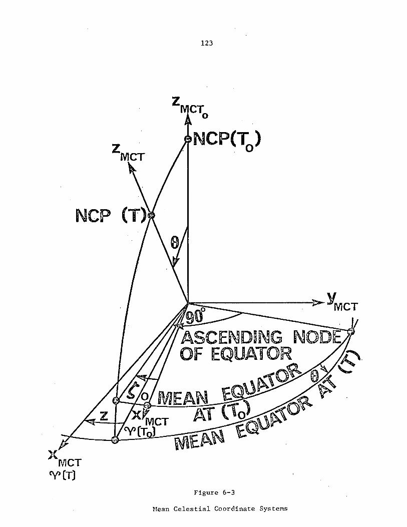
123
NCP (T)
~----. ~YMCT
Figure 6-3
Mean Celestial Coordinate Syste~s
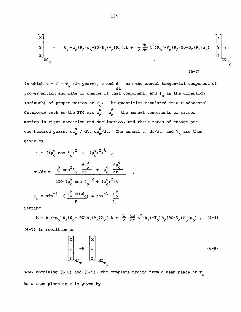
124
x
y =
(6-7)
in which t = T - T (in years), ~ and dV are the annual tangential component of o dt
proper motion and rate of change of that component, and W is the direction o
(azimuth) of proper motion at T. The quantities tabulated in a Fundamental o a 0
Catalogue such as the FK4 are ~o ' Vo ' the annual components of proper
motion in right ascension and declination, and their rates of change per
d a cS one hundred years, Vo / dt, d~o/dt. The.~nual~, d~/dt, and Wo are then
given by
dV/dt =
Setting
d a ~o -- + dt
a ( ~o (080 0 ) = -1 cos
V
(6-7) is rewritten as
x X
y =M y
z MCT o
1 2
,
Now, combining (6-6) and (6-9), the complete update from a mean place at T o
to a mean place at T is given by
(6-8)
(6-9)
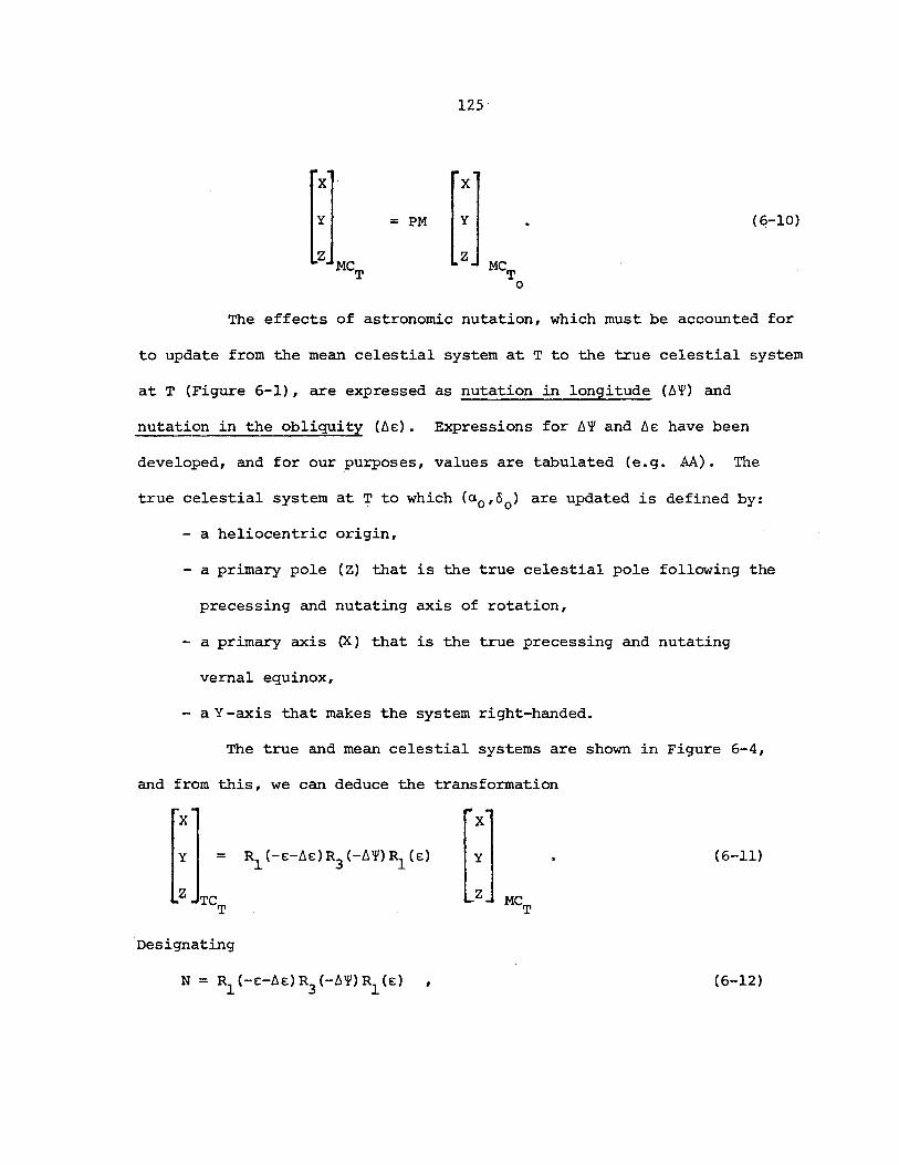
x
Y = PM
z
125'
x
Y
Z
(6-10)
The effects of astronomic nutation, which must be accounted for
to update from the mean celestial system at T to the true celestial system
at T (Figure 6-1), are expressed as nutation in longitude (6~) and
nutation in the obliquity (6E). Expressions for 6~ and 6E have been
developed, and for our purposes, values are tabulated (e.g. AA). The
true celestial system at T to which (ao'oo) are updated is defined by:
a heliocentric origin,
- a primary pole (Z) that is the true celestial pole following the
precessing and nutating axis of rotation,
- a primary axis ~) that is the true precessing and nutating
vernal equinox,
- a Y-axis that makes the system right-handed.
The true and mean celestial systems are shown in Figure 6-4,
and from this, we can deduce the transformation
x
Y
Z
=
TCT
. Designating
N = ~(-E-6E)R3(-6~)R1(E) ,
x
Y
Z
(6-11)
(6-12)
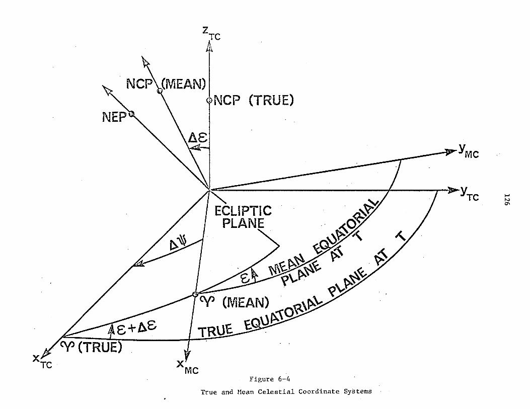
ZTC A
NCP\JMEAN) "NCP (TRUE)
~ ~c YTC
ECLIPTIC PLANE
Figure 6-4
True and Uean Celestial Coordinate Systems
...... N 0\
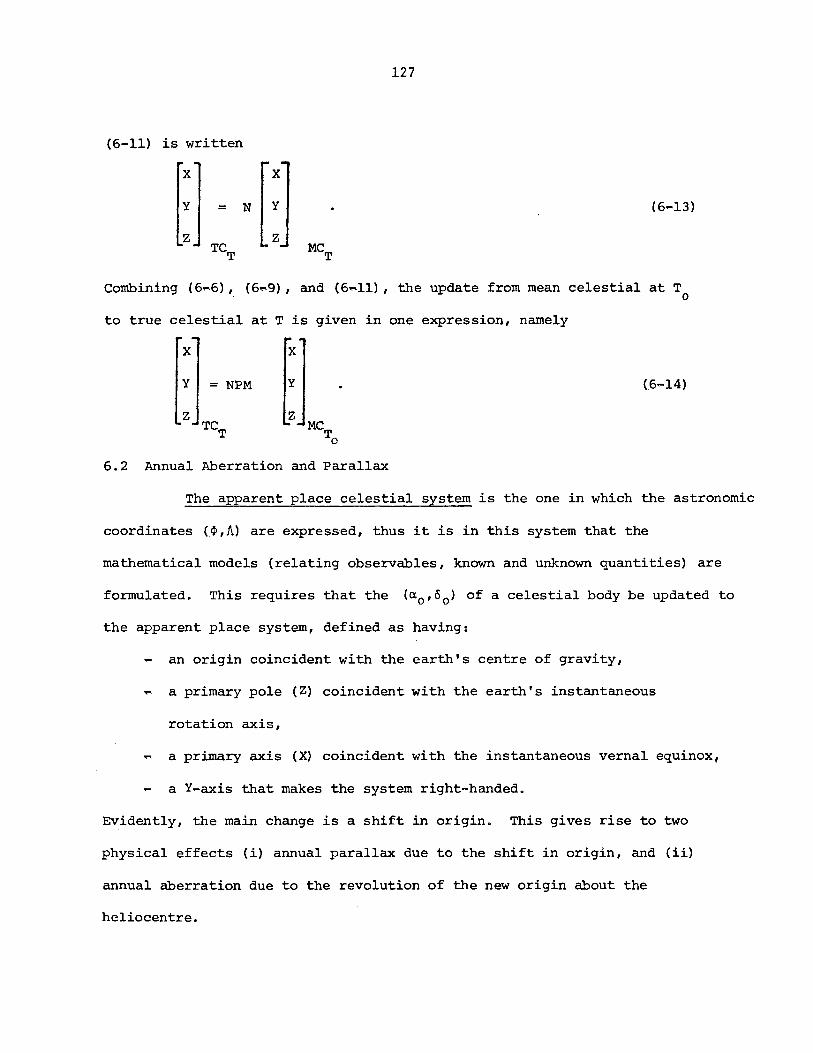
127
(6-11) is written
x x
Y = N Y (6-13)
Z Z
Combining (6~6), (6~9), and (6~11), the update from mean celestial at T o
to true celestial at T is given in one expression, namely
x x
Y = NPM Y
Z Z
6.2 Annual Aberration and Parallax
The apparent place celestial system is the one in which the astronomic
coordinates (41, h) are expressed, thus it is in this system that the
mathematical models (relating observables, known and unknown quantities) are
formulated. This requires that the (no'oo) of a celestial body be updated to
the apparent place system, defined as having:
- an origin coincident with the earth's centre of gravity,
~ a primary pole (Z) coincident with the earth's instantaneous
rotation axis,
~ a primary axis (X) coincident with the instantaneous vernal equinox,
a Y-axis that makes the system right-handed.
Evidently, the main change is a shift in origin. This gives rise to two
physical effects (i) annual parallax due to the shift in origin, and (ii)
annual aberration due to the revolution of the new origin about the
heliocentre.
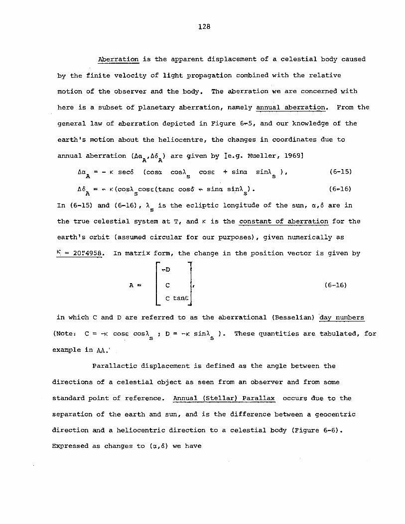
128
Aberration is the apparent displacement of a celestial body caused
by the finite velocity of light propagation combined with the relative
motion of the observer and the body. The aberration we are concerned with
here is a subset of planetary aberration, namely annual aberration. From the
general law of aberration depicted in Figure 6~5, and our knowledge of the
earth's motion about the he1iocentre, the changes in coordinates due to
annual aberration CflaA,MA) are given by Ie.g. Mueller, 1969]
fla = - K seco A
(cosa cosA s
cose + sina
flo = .... K (cosh cose [tane coso· ..... s·ina sin·h ). A . s . s
sin>.. ) , . s (6-15)
In (6~l5) and (6~16), A is the ecliptic longitude of the sun, a,o are in s
the true celestial system at T, and K is the constant of aberration for the
earth's orbit (assumed circular for our purposes), given numerically as
~ = 20~4958. In matrix form, the change in the position vector is given by
...-D
A= c (6-16)
C tans
in which C and D are referred to as the aberrational (Besselian) 'day numbers
(Note: C = -K cose cos>.. J D = -K sinA ). These quantities are tabulated, for s s
example in M:
Parallactic displacement is defined as the angle between the
directions of a celestial Object as seen from an observer and from some
standard point of reference. Annual (Stellar) Parallax occurs due to the
separation of the earth and sun, and is the difference between a geocentric
direction and a heliocentric direction to a celestial body (Figure 6-6).
Expressed as changes to (a,o) we have
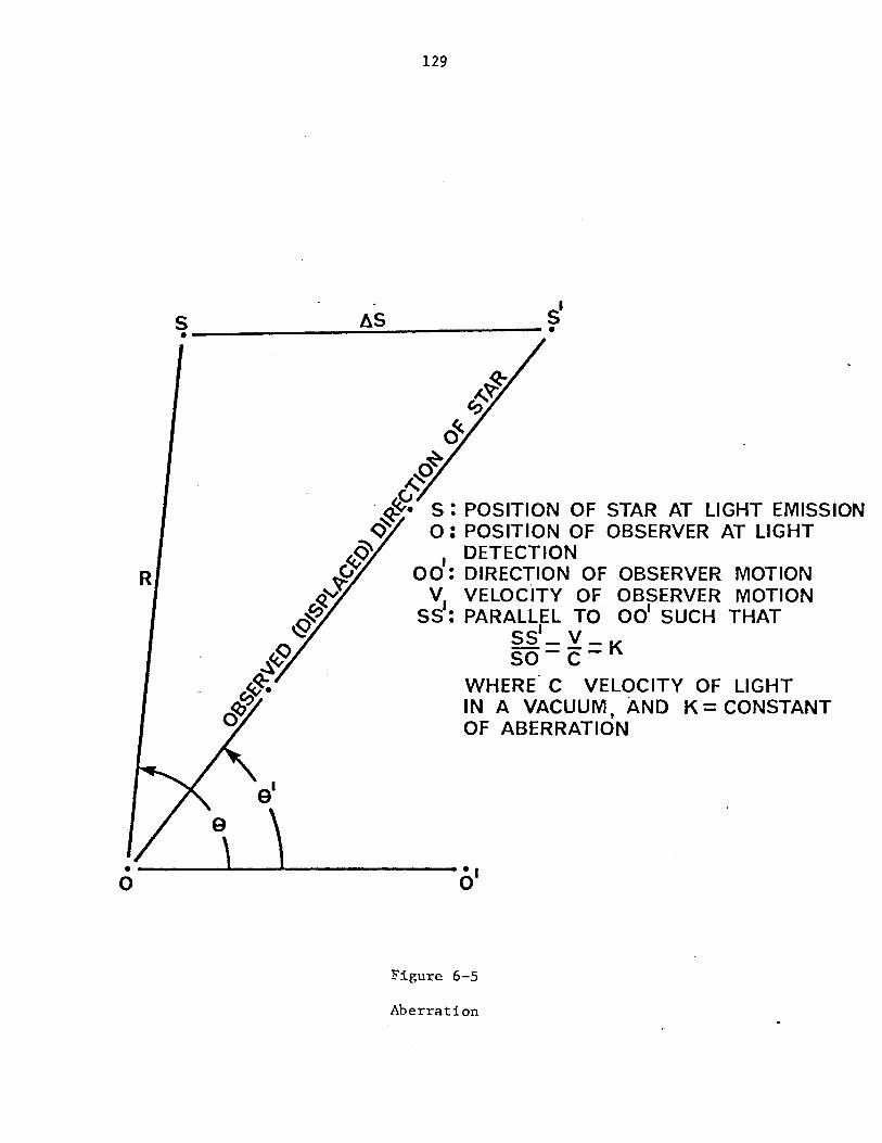
R
129
51 ~ ____________ =A~5----------_.
S-~ ~
O~ ~ i'- S: POSITION OF STAR AT LIGHT EMISSION
Q' 0: POSITION OF OBSERVER AT LIGHT 9' DETECTION
~l<; od: DIREC~ION OF OBSERVER MOTION 9." VI VELOCITY OF OBSERVER MOTION
r.:>~ S5: PARALLEL TO 00' SUCH THAT ~ 5SI _ V_
~ SO-C- K ~
$. g,(,j
o WHERE' C VELOCITY OF LIGHT IN A VACUUM, AND K = CONSTANT OF ABERRATION
----------~-----------·I o
Figure 6-5
Aberration
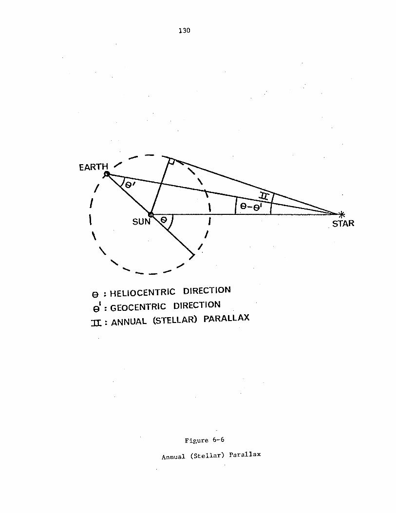
I I \ \ ,
"
130
"'" '" -- ......
\ I
I
9 : HELIOCENTRIC DIRECTION
9' : GEOCENTRIC DIRECTION
:II : ANNUAL (STELLAR) PARALLAX
Figure 6-6
Annual (Stellar) Parallax

131
flo. = II {COSo. COSE sin}, ..... sino. cos). ) seco p . s s (6",,17)
flo = II (coso sinE sinA. .. coso. sino COSA. .. sino. sino COSE sinA. ), (6-18) p s s s
in which the new quantity II is the annual (stellar) p!irallax. II is a small
quantity - for the nearest star it is 0~76. As for the computation of the
effects of aberration, 0.,0 in {6-17} and (6-18) are in the true celestial
system at T. Using the Besselian Day Numbers C and D, the changes in the
position vector are given by
-c seCE
R= -D COSE (II/K)
-D sinE
To update (0.,0) from the True Celestial system at T to the Apparent Celestial
system at T, we write the expression
x x
y = A + R + y (6-20)
z z
Finally, the complete update from Mean Celestial system at T to Apparent o
Celestial at T is given by the expression
x x
y = A + R + NPM y
z z A.P· T MCT
o
(6-21)
This entire process is summarised in Figure 6-7, and all symbols used in
Figure 6-7 are explained in Table 6-1.
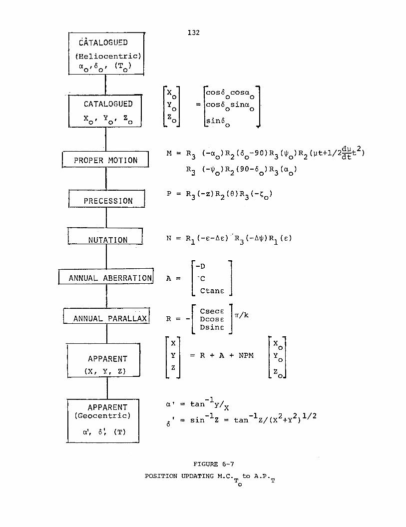
.'
I
I
l
CATALOGUED ~He1iocentric)
ao'tSo ' (To)
-
CATALOGUED
XO' Yo' Z 0
PROPER MOTION
PRECESSION
NUTATION
-,
132
costS cosa o 0 = costS sina o 0
sintSo
M = R3 (-ao)R2(tSo-90)R3(~o)R2(~t+1/2~~t2)
R3 (-~o)R2(90-tSo)R3(ao)
ANNUAL ABERRATIONl A = ntanE]
ANNUAL PARALLAXt R = [ CseCE ] ~/k - Dcose:
APPARENT (X, Y, Z)
APPARENT (Geocentric)
a', tS~ (T)
Dsine:
X X 0
Y = R + A + NPM Y 0
Z Zo
-1 a' = tan y/x
= sin-1Z = tan-1z/(x2+y2)1/2
FIGURE 6-7
POSITION UPDATING M.e. to A.P. T To
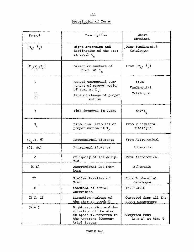
133
Description of Terms
Symbol Description Where Obtained
(a , o ) Right ascension and From Fundamental 0 0 declination of the star Catalogue
at epoch T 0
(X , Y ,Z ) Direction numbers of From (a , 0 ) 000 0 0
star at T 0
II Annual Tangential com- From ponent of proper motion Fundamental of star at T •
dll 0 Catalogue
Rate of change of proper dt motion
t Time interval in years t=T-T 0
ljJo Direction (azimuth) of From Fundamental proper motion at T Catalogue
0
(1;;0' z, e) Precessional Elements From Astronomical
(6ljJ, 6£) Nutational Elements Ephemeris
£ Obliquity of the eclip- From Astronomical tic
(C,D) Aberrational Day Num- Ephemeris bers
II Stellar Parallax of From Fundamental Star Catalogue
K Constant of annual K=20".4958 Aberration
(X,Y, Z) Direction numbers of Computed from all the the star at epoch T above parameters
! "1 '1 (a,o ) Right ascension and de-
clination of the star at epoch T, referred to Computed from the Apparent (Geocen- (X,Y,Z) at time T tric) System.
TABLE 6-1
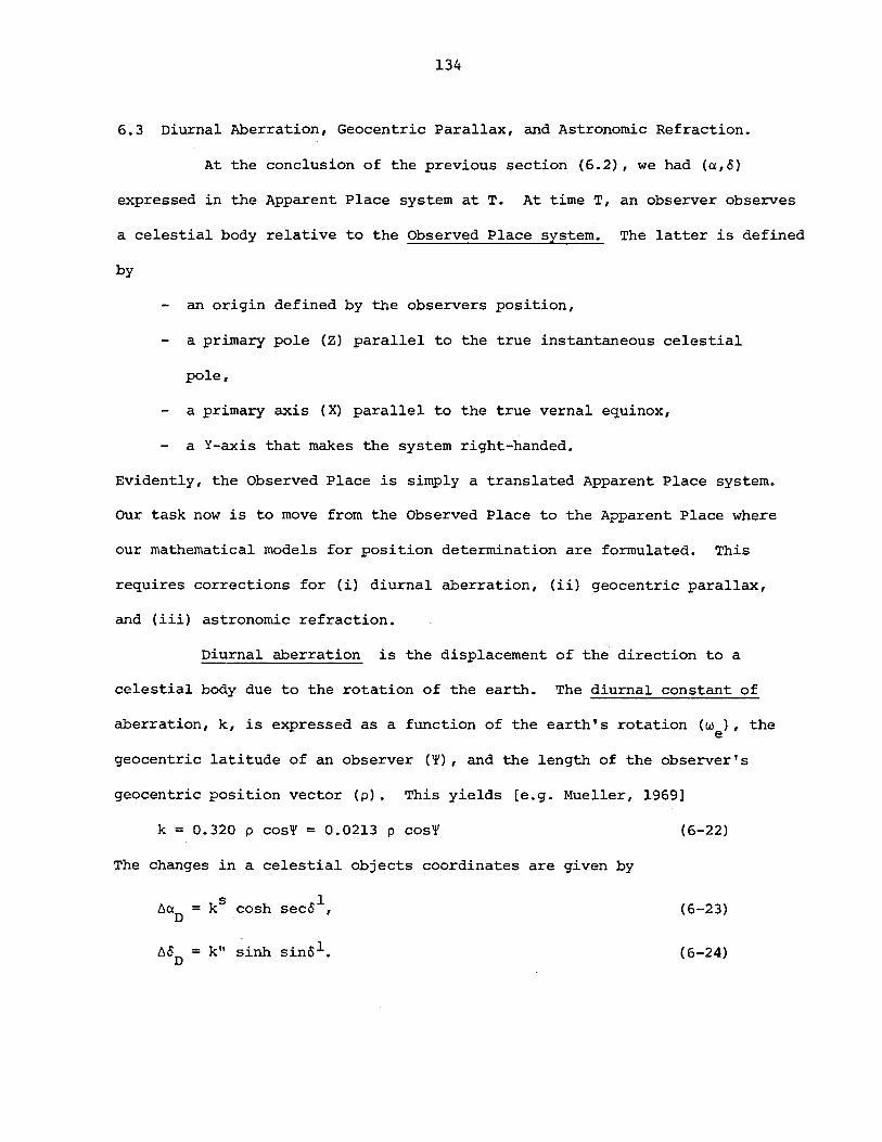
134
6.3 Diurnal Aberration, Geocentric Parallax, and Astronomic Refraction.
At the conclusion of the previous section (6.2), we had (a,~)
expressed in the Apparent Place system at T. At time T, an observer observes
a celestial body relative to the Observed Place system. The latter is defined
by
an origin defined by the observers position,
a primary pole (Z) parallel to the true instantaneous celestial
pole,
a primary axis (X) parallel to the true vernal equinox,
a Y-axis that makes the system right-handed.
Evidently, the Observed Place is simply a translated Apparent Place system.
Our task now is to move from the Observed Place to the Apparent Place where
our mathematical models for position determination are formulated. This
requires corrections for (i) diurnal aberration, (ii) geocentric parallax,
and (iii) astronomic refraction.
Diurnal aberration is the displacement of the direction to a
celestial body due to the rotation of the earth. The diurnal constant of
aberration, k, is expressed as a function of the earth's rotation (00 ), the e
geocentric latitude of an observer (~), and the length of the observer's
geocentric position vector (p). This yields [e.g. Mueller, 1969]
k = 0.320 p cos~ = 0.0213 p cos~ (6-22)
The changes in a celestial objects coordinates are given by
6aD kS cosh 1 = sec6 , (6-23)
~6D = k" sinh sin6 l • (6-24)
135
The convention adopted here for signs is
~aD = aAP aOp , (6-25) T . T
~<5D = <5AP <50P • (6-26) T T
This same convention applies to the corrections for geocentric parallax and
astronomic refraction that are treated next.
Geocentric parallax is the difference between the observed
topocentric direction and the required geocentric direction (Figure 6-8).
The changes, expressed in terms of the celestial objects right ascension and
declination are
~aG = - n sinh cosecz cos~ sec<5' (6-27)
n (sin~ cosecz sec<5' - tan <5 , cotz). (6-28)
It should be noted that for celestial bodies other than the sun, ~aG'
~<5G are so small as to be negligible.
Astronomic refraction is the apparent displacement of a celestial object
lying outside our atmosphere that results from light rays being bent in passing
through the atmosphere. In general, the light rays bend downward, thus a
celestial object appears at a higher altitude than is really true
(Figure 6-9). The astronomic refraction angle is defined by
~z = z - z' R
(6-29)
in whichz' is the observed zenith distance, z is the corrected zenith distance.
The effects on a,<5 are
~a = - ~z sinh cosec z I cos~ sec<5' R R (6-30)
~<5R = - ~zR (sin~ cosec Zl sec<5 1 - tan<5 1 cot Zl). (6-31)
~zR values are usually tabulated for some standard temperature and pressure
(usually 760mm Hg, T = 10°C, relative humidity 60%) • Corrections to those
values are obtained through determinations of temperature, pressure, and
GEOCENTRE
136
Figure 6-8
STAR
1T: GEOCENTRIC PARALLAX
Z· : MEASURED DIRECTION
Z : GEOCENTRIC DIRECTION
Geocentric Parallax
-- -- ....... ""'"- ......
"'" " "
137
Figure 6-9
\ DIRECTION
\ \ \ \ \ \ ,
Astronomic Refraction
u .. 1/ to S
to S
138
relative humidity at the time of observation (T)o
Finally, we can write the expressions for the right-ascension
and declination of a celestial body as
a = ~ -AoPo T AoPo T (~aD + ~ap + ~~ (6-32)
0 = 0' - (~OD + ~Op + ~OR) , (6-33) AoPo T A.P· T
in which a' and 0' refer to the Apparent Place coordinates obtained from ~ ~
equation (6-21). This process is summarized in Figure 6-10.
In closing this section, the reader should note the following. It
is common practice in lower-order astronomical position and azimuth
determinations to correct the observed direction z' for both geocentric
parallax and refraction rather than use (6-32) and (6-33) above. Thus, in
our math models we use
z = z' - (~z + ~z ) R P
(6-34)
~zp, the correction to a zenith distance due .. to geocentric parallax,
is tabulated (e.g. SALS). Note that the effects of diurnal aberration are
neglected.
6.4 Polar Motion
The final problem to be solved is the transformation of astronomically
determined positional coordinates (~,A) from the Apparent Place celestial
system to the Average Terrestrial coordinate system. This involves two
steps: (i) transformation of aAP ' 0AP (Apparent Place) to Instantaneous
Terrestrial and (ii) transformation of WIT' AIT (Instantaneous Terrestrial) to
Average Terrestrial.
In the first step, we are moving from a non-rotating system to a
coordinate system that is rotating with the ~arth. The Instantaneous
139
APPARENT PLACE
(GEOCENTRIC)
I ~ =rep-(A~ +Arx. +A<X)
AP AGO R
6 =61 -(~6 +A6 +AS ) AP AP G 0 R
"
DIURNAL ABERRATION
AQh,llSD
~
GEOCENTRIC PARALLAX A~,A6G
~
ASTRONOMIC REFRACTION A~,A6R
~
OBSERVED PLACE
(TOPOCENTRIC)
Figure 6-10
Observed to Apparent Place .
140
Terrestrial (IT) system is defined by
-a geocentric origin,
-a primary pole (Z) that coincides with the instantaneous terrestrial pole,
-a primary axis (X) that is the intersection of the Greenwich Mean Astronomic Meridian and Instantaneous equatorial planes,
-a Y-axis that makes the system right-handed.
Comparing the definitions of the A.P. and I.T. systems, we see that
the only difference is in the location of the primary axis, and futhermore,
that XIT is in motion. Recalling the definition of sidereal time, we see
that the A.P. and I.T. systems are related through GAST (Figure 6-11), namely
X X
Y = R3 (GAST) Y (6-35)
z Z IT AP
in which
X cos~ coscx X cos<S coso.
Y = coso sino; Y = coso sino. , (6.36)
Z APT
sino APT
z sino
or, using a spherical approximation of the earth
X cos~ cosh
Y = cos~ sinh
I.T. z
IT sin~
The reader should note that this transformation is usually (6-35)
carried out in an implicit fashion within the mathematical models for
position and azimuth determination rather than explicitly as is given here
(see, for example, Chapters 8 and 9). The results that one obtains are then
Figure 6-11
Transformation of Apparent Place
To Instantaneous Terrestrial
System
142
~,h,A, all expressed in an Instantaneous Terrestrial coordinate system. The
final step is to refer these quantities to the Average Terrestrial coordinate
system.
The direction of the earth's instantaneous rotation axis is moving
with respect to the earth's surface. The motion, called polar motion, is counter
c1ockWis-e~ 'quas±--frt'egi:J.lar, ha~".:m aml'litude ,of'about· 5m',and' a period of
approximately 430 m.s.d. The motion is expressed in te~ of the
position of the instantaneous rotation axis with respect to a reference point
fixed on the earth's crust. The point used is the mean terrestrial pole for
the interval 1900-1905, and is called the conventional International Origin
(C.I.O.).
The Average Terrestrial (AT) coordinate system is the one which we
would like to refer astronomic positions (~,h). This system differs in
definition from the I.T. system only in the definition of the primary pole -
the primary A.T. pole is the C.I.O. Referring to figure 6-12, we can easily
see that
x x
y = R_ (-x) R (-y) 2 p 1 P
y (6-37)
z AT
z LT.
Using a spherical approximation for the earth which is adequate for this
transformation, one obtains [Mueller, 1969]
cos~ cosh
cos~ sinh
sin~ A.T.
= R_{-x ) R (-y ) -~ P 1 P
cos~ cosh
cos~ sinh
sin~
(6-38)
I.T.

143
y _0-----.--------... CIO y __ ---------.. CIO
I I . I
xp I I I I
~ ... ------------,/' Yp
INSTANTANEOUS TERRESTRIAL POLE
TRANSFORMATION FROM INSTANTANEOUS ·TO AVERAGE
TERRESTRIAL SYSTEM.
FIGURE 6-12
x
144
Specifically, one obtains after some manipulations, the two equations
[Mueller, 1969]
~~ = ~AT - ~IT = yp sinAIT - xp cosAIT (6-39)
~A = AAT - AIT = -(xp sinAIT + yp cosAIT) tan~IT (6-40)
The effect of polar motion on the astronomic azimuth is expressed as
[Mueller, 1969]
(6-41)
The complete process of position updating, and the relationship
with all celestial coordinate systems is depicted in Figure 6-13. The
relationships amongst all of the coordinate systems used in geodesy, with
celestial systems in perspective, is given in Figure 6-14.
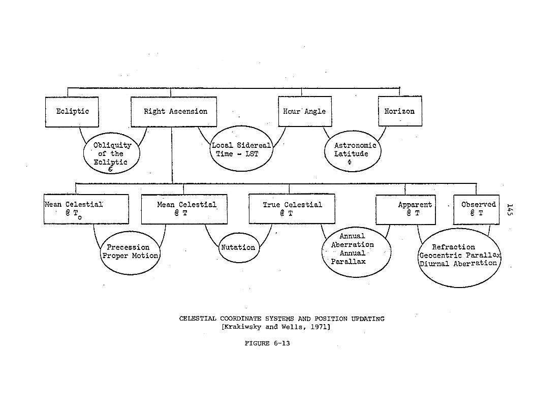
Ecliptic
Mean Celestial" @ To
Right Ascension
Mean Celestial @ T .
Hour'Angle
"
True Celestial @ T
CELESTIAL COORDINATE SYSTEMS AND POSITION UPDATING [Krakiwsky and Wells, 1971]
FIGURE 6-13
Horizon
Apparent @ T
Observed @ T
I-' -I::'VI
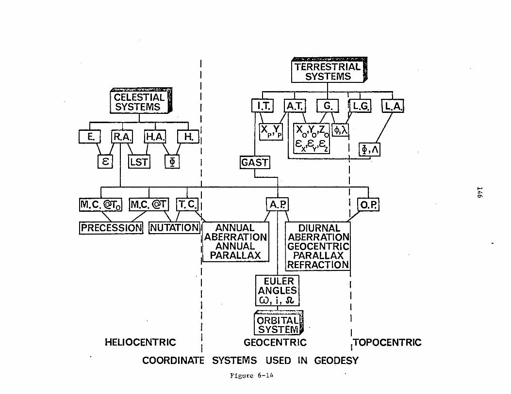
CELESTIAL SYSTEMS
TERRESTRIAL SYSTEMS
DIURNAL ABERRATION GEOCENTRIC
PARALLAX REFRACTION
-EULER ANGLES CU, i, Sl,
i
ORBITAL" SYSTEI\~, I
HELIOCENTRIC GEOCENTRIC ITOPOCENTRIC
COORDINATE SYSTEMS USED IN GEODESY
FiBure 6-1L..
......
. ~ 0'\
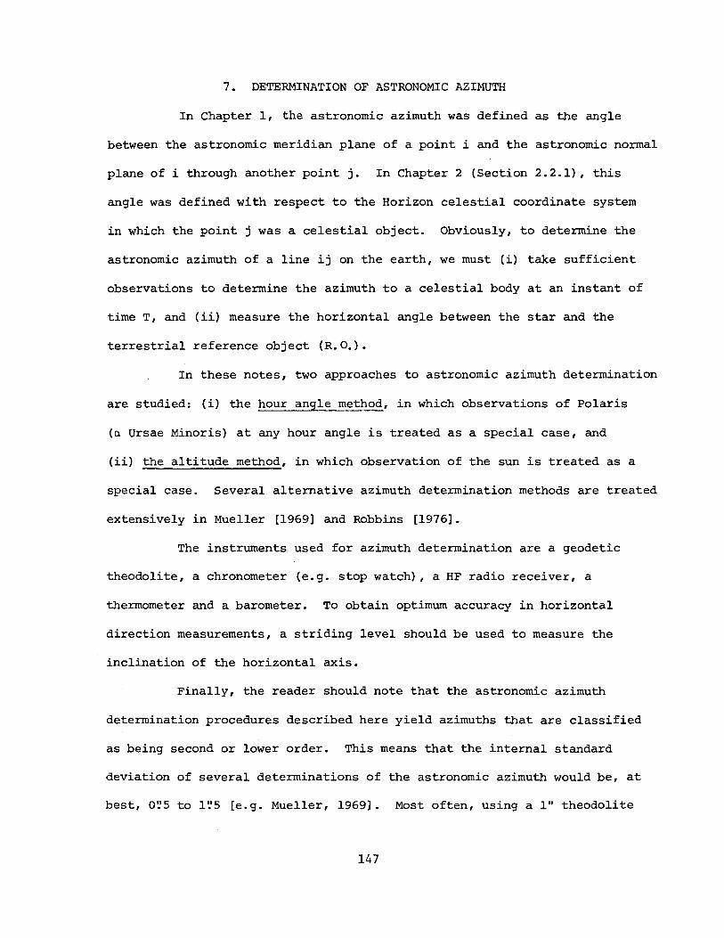
7. DETERMINATION OF ASTRONOMIC AZIMUTH
In Chapter 1, the astronomic azimuth was defined as the angle
between the astronomic meridian plane of a point i and the astronomic normal
plane of i through another point j. In Chapter 2 (Section 2.2.1), this
angle was defined with respect to the Horizon celestial coordinate system
in which the point j was a celestial object. Obviously, to determine the
astronomic azimuth of a line ij on the earth, we must (i) take sufficient
observations to determine the azimuth to a celestial body at an instant of
time T, and (ii) measure the horizontal angle between the star and the
terrestrial reference object (R.O.).
In these notes, two approaches.to astronomic azimuth determination
are studied: (i) the hour angle method, in which observations of Polaris
(a Ursae Minoris) at any hour angle is treated as a special case, and
(ii) the altitude method, in which observation of the sun is treated as a
special case. Several alternative azimuth determination methods are treated
extensively in Mueller [1969] and Robbins [1976].
The instruments·used for azimuth determination are a geodetic
theodolite, a chronometer (e.g. stop watch), a HF radio receiver, a
thermometer and a barometer. To obtain optimum accuracy in horizontal
direction measurements, a striding level should be used to measure the
inclination of the horizontal axis.
Finally, the reader should note that the astronomic azimuth
determination procedures described here yield azimuths that are classified
as being second or lower order. This means that the internal standard
deviation of several determinations of the astronomic azimuth would be, at
best, O~5 to 1~5 [e.g. Mueller, 1969]. Most often, using a 1" theodolite
147
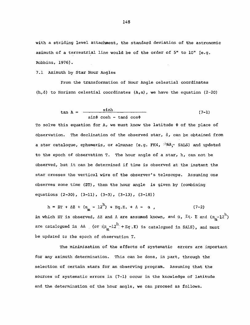
148
with a striding 1eve1attachment, the standard deviation of the astronomic
azimuth of.aterrestrial line would be of the order of 5" to 10" [e.g.
Robbins, 1976].
7.1 Azimuth by Star Hour Angles
From the transformation of Hour Angle celestial coordinates
(h,o) to Horizon celestial coordinates (A,a), we have the equation (2-20)
tan A = sinh. (7-1) sin~ cosh - tano cos~
To solve this equation for A, we must know the latitude ~ of the place of
observation. The declination of the observed star, 0, can be obtained from
a star catalogue, ephemeris, or almanac (e.g. FK4, ~Mr SALS) and updated
to the epoch of observation T. The hour angle of a star, h, can not be
observed, but it can be determined if time is observed at the instant the
star crosses the vertical wire of the observer's telescope. Assuming one
observes zone time (ZT), then the hour angle is given by (combining
equations (2-30), (3-11), (3-3), (3-13), (3-18»
h h = ZT + AZ + (a - 12 ) + Eq.E. + A - a, m
(7-2)
in which ZT is observed, AZ and A are assumed known, a,nd .0., .Eq. E and (~~ .-12h) m
are cata10guedin AA. . (or \(~m~12h:+_Eq·.E)iS ca.ta1ogued in SALS), and must
be updated to the epoch of observation T.
The minimization of the effects of systematic errors are important
for any azimuth determination. This can be done, in part, through the
selection of certain stars for an observing program. Assuming that the
sources of systematic errors in (7-1) occur in the knowledge of latitude
and the determination of the hour angle, we can proceed as follows.
149
Differentiation of (7-1) yields.
dA = sinA cotz d~ + cos~ (tan~ - cosA cotz)dh. (7-3)
Examination of (7-3) yields the following:
(i) ° ° when A = 0 or 180 , the effects of d~ are~9liminated,
(ii) when tan~ = cosA cotz, the effects of dh are "eliminated.
Thus, if a star is observed at transit (culmination), the effects of d~ are
minimized, while if a star is observed at elongation (parallactic angle
° p = 90 ), the effects of dh are minimized. Of course, it is not possible
to satisfy both conditions simultaneously; however, the effects will be
elliminated if two stars are observed such that
sinAl cotz1" = -sinA2 cotz2 (7-4)
2tan~ - (COSAl cotzl + COSA2 cotz2) = 0 (7-5)
As a general rule, then, the determination of astronomic azimuth using the
hour angle method must use a series of star pairs that fulfill conditions
(7-4) and (7-5). This procedure is discussed in detail in, for example,
Mueller [1969] and Robbins [1976].
A special case can be easily made for cicumpolar stars, the most
well-known of which in the northern hemisphere is Polaris (a. Ursae'Minoris ).
When ~ > 15° Polaris is easily visible and directions to it are not affected
unduly by atmospheric refraction. Since A = 0°, the error d~ is
eliminated. Furthermore, since in (7-3), the term [Robbins, 1976]
cos~ (tan~ - cosA coti) = cos~ cosz cosp, (7-6)
then when ~ = 90° I the effects of dh are elliminated. Then Polaris can be
observed at any hour angle for the determination of astronomic azimuth by
the hour angle method.
150
A suggested observing sequence for Polaris is as follows
[Mueller, 1969]:
(i) Direct on R.O., record H.C.R.,
(ii) Direct on Polaris, record H.C.R. and T,
(iii) Repeat (ii),
(iv) Repeat (i)~ ,
(v) Reverse telescope and repeat (i) through (iv).
The above observing sequence constitutes one azimuth determination;
eight sets are suggested. Note that if a striding level is 'used, readings
of both ends of the level (e.g. e and w for direct, e " and Wi for reverse)
should be made and recorded after the paintings on the star. An azimuth
correction, for each observed set,is then given by [Mueller, 1969]
I:J.A" = d" ( (w + Wi) - (e + e ' ) ) cotz (7-7) 4
in which d is the value in arc-seconds of each division of the striding
level.
Briefly, the computation of astronomic azimuth proceeds as
follows:
(i) for each of the mean direct and reverse zone time (ZT) readings
of each set on Polaris, compute the hour angle (h) using (7-2),
(ii) using (7-1), compute the astronomic azimuth A of Polaris for
each of the mean direct and reverse readings of each set,
(iii) using the mean direct and mean reverse H.C.R.'s of each set on
Polaris and the R.O., compute the astronomic azimuth of the
terrestrial line,
(iv) the mean of all computed azimuths (two for each observing sequence,
eight sets of observations) is the azimuth of the terrestrial line,

151
(v) computation.of the standard deviation of a single azimuth
determination and of the mean azimuth completes the computations.
computations may be shortened somewhat by (i) using the mean
readings direct and reverse for each set of observed times and H.C.R.'s
(e.g. only 8 azimuth determinations) or (ii) using the mean of all time and
H.C.R.'S, make one azimuth determination. If either of these approaches
are used, an azimuth correction due to the non-linearity of the star's
path is required. This correction (6A ) is termed a second order c
curvature correction [Mueller, 1969]. It is given by the expression
" A c = n I
i=l m. ~
(7-8)
in which n is the number of observations that have been meaned (e.g. 2
for each observing sequence (direct and reverse), 16 for the total set of
observations (8 direct, 8 reverse». The term CA is given by
= tanA
. 2h s~n
2 2 cos h - cos, A
2 cos A (7-9)
in which the azimuth A is the azimuth of the star (Polaris) computed
without the correction. The term m. is given as ~
2 mi = ~"[i sin 2" ,
where
"[i = (T. - T ) , ~ 0
and Tl + T2 + .... + T
T n = 0 n
(7-10)
(7-11)
(7-12)
If, when observing Polaris, the direct and reverse readings are
made within 2m to 3m , the curvature correction ~A will be negligible and c
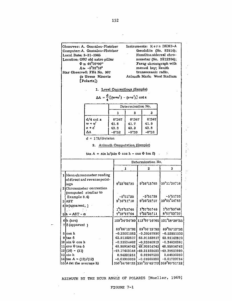
152
Observer: A. Gonzalez-Fletcher Computer: A. Gonzalez-Fletcher Local Date: 3-31-1965
Instruments: K ern DKM3-A theodolite (No. 82514); Hamiltonsidereal chronometer (No. 2EI2304); Favag chronograph with manual key; Zenith transoceanic radio.
Location: OSU old astro pillar tit e! 40°00'00" Ae! -51132~0·
Star Observed: FK4 No. 907 (a Ursae Minoris [Polaris])
Azimuth Mark: West Stadium
1. Level Corrections (Sample)
d [' , J AA = 4' ,(w+w) - (e+e) cotz
Determination No.
1 2 3
d/4 cot z 0'!347 0'!347 0'!347 w+vI 41.8 41.7 41.9 e+ff 43.3 43.3 42.8 AA -0'!52 -0'!59 -0'!31
d = 1 '!6/division
2. Azimuth Computation (Sample)
tan A == sin h/ (sin If, cos h - cOs c;l) tan 6) ..
1 j\Iean chronometer reading I ~f direct and reverse point-1O"'S
12 Chronometer correction (computed similar to Example 8.4)
3 AST 4 a(8.J?parentiJ
,,',~ .'
5 h == AST - a
6 h (arc) 7 6 (apparent 1 .
8 cos h 9 tan 6
10 sin'cp cos h 11 cos 9 tan 6 12 (10) - (11) 13 Sill h 14 tan A == (13)/(12) 15 A (at the average h)
Determination No.
1 2 3
91:22:02~35 9~6t;,13~85 101111 "38~ 16
-5c51~25 -5"51!28 -5rsl~33
9hI6:11~ 10 9"s0"22~ 57 10b05"46~83
Ih57"53~46 Ih57"53~46 ih57rs3~46 7h18c17~64 7~2"29~11 8"o7=S3~37
109~4'24':60 113°07'16'!65 121°58'20'!55
89°06'12'!92 89°06'12':92 89006'12'!92 -0.33501582 -0.39267890 -0.529510321 63.91162817 63.91162817 63.91162812 -0.21534402 -0.25240913 -0.3403626; I 48.95914742 48-:95914742 48.95914742
-49.17449144 -49.21155655 -49.299510091' 0.94221251 0.91967535 0.84830350
-0.01916059 -0.01868820 -0.01720714 i 35S054'08'!33 35S055 '45'!73 359°00'51'!12!
AZIMUTH BY THE HOUR ANGLE OF POLARIS [Mueller, 1969]
FIGURE 7-1
!"\
" 0'
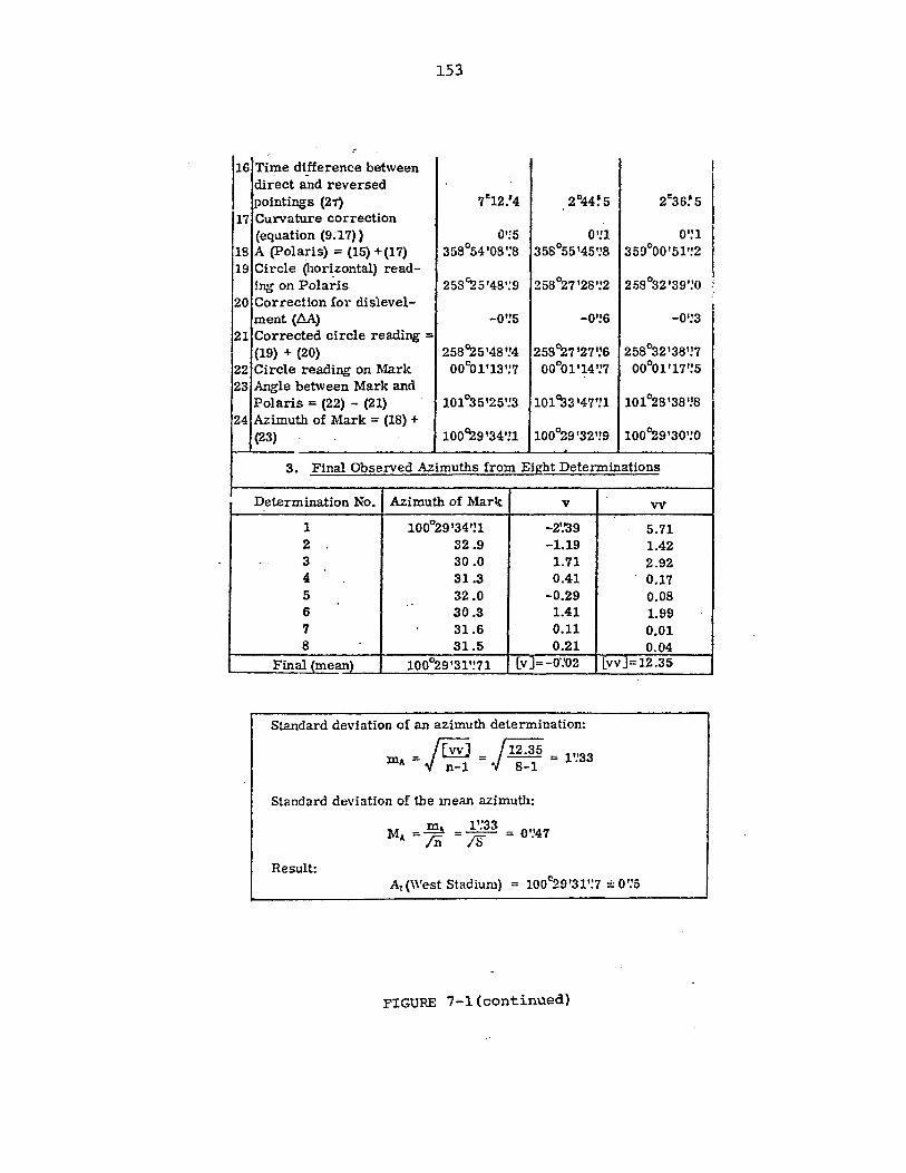
16
17
18 19
20
21
22 23
24
153
Time difference between direct and reversed ~)ointings (21) 7"12.'4 2D44~5 2~6~5 Curvature correction (equation (9;17» 0'15 O'!1 0':1 A (polaris) = (15) + (17) 35So54 'OS ':S 35S055 '45':S 359000'51'!2 Circle (hor~zontal) read-ing on Polaris 25So..zS '48':9 258°27'28':2 258°32'39'!0 Correction for dislevel-ment (AA) -O'!5 -0':6 -0':3 Corrected circle reading = (19) + (20) 25S~5'4S'!4 25S~7 '27':6 258°32'3S'!7 Circle reading on Mark 00~1'13':7 00°01 '14'!7 00001'17'!5 Angle between Mark and Polaris = (22) - (21) 101°35'25'!3 101~3'47'!1 101°28 '3S '!8 . Azimuth of Mark = (18) + (23) .. 100~9'34'!1 100~9'32'!9 100~9'30'!0
3. Final Observed Azimuths from Eight Determinations
Determination No. Azimuth of Marlt v
- .
1 100°29 '34 '!1 -2'.'39 2 32.9 -1.19 3 30.0 1.71 4 31.3 0.41 5 32.0 -0.29
." 6 30.3 1.41 7 31.6 0.11 8 31.5 0.21
Final (mean) 100°29'31':71 [v]=-O'!02
Standard deviation of an azimuth det.ermination:
= jrvv] = J12.35 = 1"33 mA n-1 8-1 .
Standard deviation of the mean azimuth:
m. 1':33 M ..--.... = 0'.'47 A=rn =18
Result:
FIGURE 7-1(continued)
vv
5.71 1.42 2.92 0.17 O.OS 1.99 0.01 0.04
[vv]=12.35
I
! i
154
could therefore be neglected [Robbins, 1976]. An example of azimuth
determination by the hour angle of Polaris is given in Figure 7-1.
Azimuth by hour angles is used for all orders of astronomic work.
The main advantages of this method are that the observer has only to
observe the star as it coincides with the vertical wire of the telescope
and since no zenith distance measurement is made, astronomic refraction has
no effect. The main disadvantages are the need for a precise time-keeping
device and a good knowledge of the observer's longitude.
Table 7-1 summerizes, for several situations, the sources of
errors and their magnitudes in the determination of astronomic azimuth by
stars hour angles.
7.2 Azimuth by Star Altitudes
Azimuth by star altitudes yields less accurate results than
azimuth by star hour angles. The two reasons for this are (i) the star
must be observed as it coincides with both the horizontal and vertical wires
of the telescope, and (ii) the altitude observation is subject to the
effects of astronomic refraction. The method does have the advantage,
however, that a precise knowledge of the observer's longitude is not
required and an accurate time-keeping device is not needed. Azimuths
determined by star altitudes are not adequate for work that requires 0A
to be 5" or less.
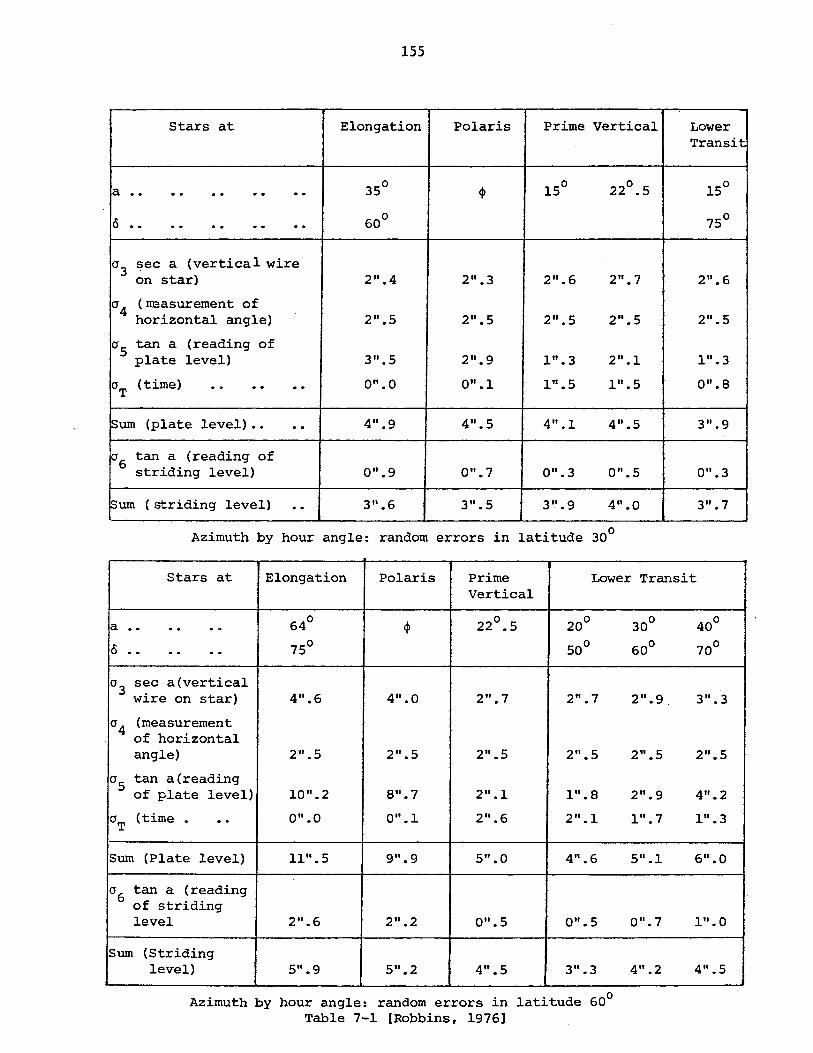
155
Stars at Elongation Polaris Prime Vertical Lower Transit
a . . . . · . · . · . 35° 4» 15° 22°.5 15°
15 . . . . · . · . · . 60° 75°
0 3 sec a (vertical wire on star) 2".4 2".3 2".6 2".7 2".6
0 4 (m=asurement of horizontal angle) 2".5 2".5 2".5 2".5 2".5
0 5 tan a (reading of plate level) 3".5 2".9 1".3 2".1 1".3
aT (time) · . · . · . 0".0 0" .1 1".5 111.5 0".8
~um (plate level) •• · . 4".9 4".5 4".1 4".5 3".9
0 6 tan a (reading of striding level) 0".9 0".7 0".3 0".5 0".3
Sum ( striding level) · . 3".6 3".5 3',' .9 4".0 3".7
Azimuth by hour angle: random errors in latitude 30°
Stars at Elongation Polaris Prime Lower Transit Vertical
a . . . . · . 64° 4» 22°.5 20°
15 . . . . · . 75° 50°
0 3 sec a(vertical wire on star) 4".6 4".0 2".7 2".7
0 4 (measurement of horizontal angle) 2".5 2".5 2".5 2".5
0 5 tan a(reading of plate level) 10".2 8".7 211.1 1".8
aT (time . . . 0".0 0" .1 2".6 2".1
Sum (Plate level) 11".5 9".9 5".0 4".6
0 6 tan a (reading of striding level 2".6 2".2 0".5 0".5
Sum (Striding level) 5".9 5".2 4".5 3".3
Azimuth by hour angle: random errors in latitude 60° Table 7-1 [Robbins, 1976]
30° 40°
60° 70°
2".9 , 3".3
2".5 2".5
211.9 4".2
1".7 1" .3
5" .1 6" .0
0".7 1".0
4".2 4".5
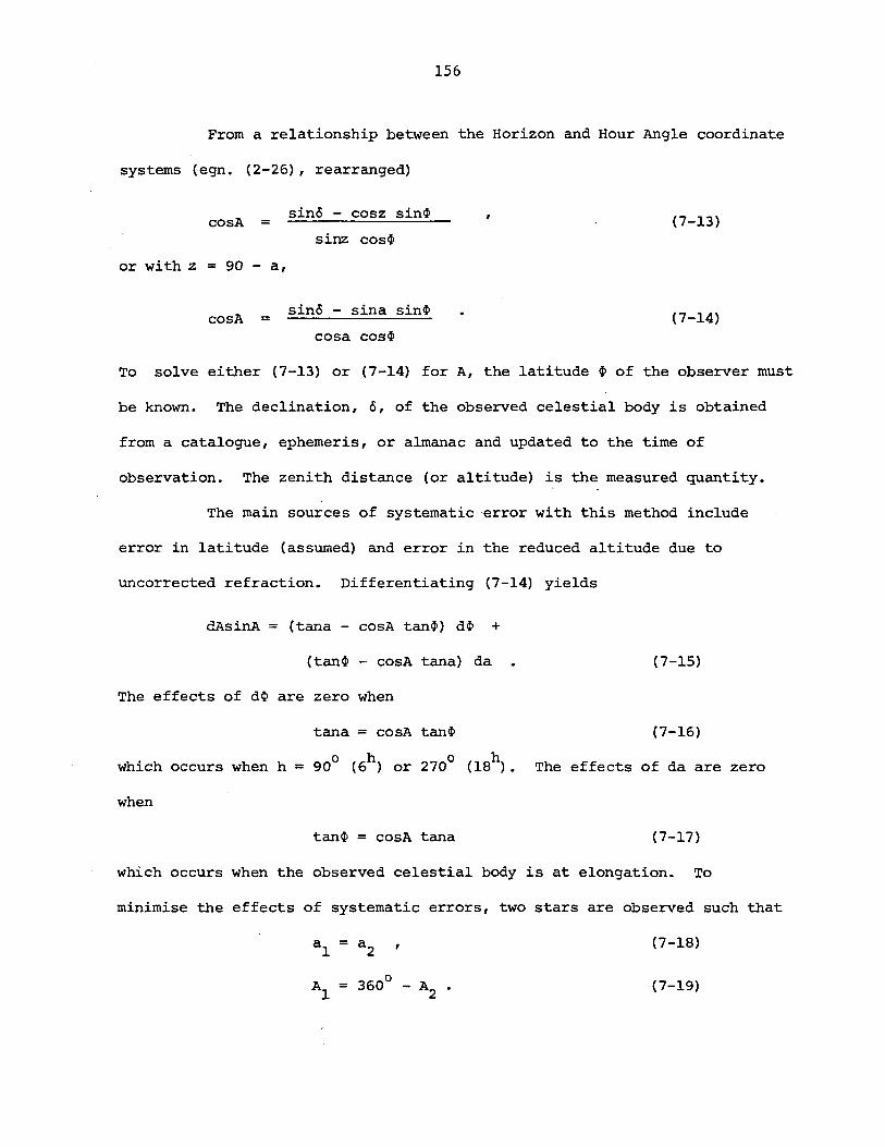
156
From a relationship between the Horizon and Hour Angle coordinate
systems (egn. (2-26), rearranged)
cosA =
or with z = 90 - a,
cosA =
sino - cosz sin4'>
sinz cos4'>
sin6 - sina sin4'>
cosa cos4'>
(7-13)
(7-14)
To solve either (7-13) or (7-14) for A, the latitude 4'> of the observer must
be known. The declination, 6, of the observed celestial body is obtained
from a catalogue, ephemeris, or almanac and updated to the time of
observation. The zenith distance (or altitude) is the measured quantity.
The main sources of systematic 'error with this method include
error in latitude (assumed) and error in the reduced altitude due to
uncorrected refraction. Differentiating (7-14) yields
dAsinA = (tana - cosA tan4'» d4'> +
(tan4'> - cosA tana) da (7-15)
The effects of d4'> are zero when
tana = cosA tan4'> (7-16)
• 0 h 0 h wh1ch occurs when h = 90 (6) or 270(18). The effects of da are zero
when
tan4'> = cosA tana (7-17)
which occurs when the observed celestial body is at elongation. To
minimise the effects of systematic errors, two stars are observed such that
a l = a2 ' (7-18)
Al = 3600 - A2 (7-19)
157
Further details on the selection of star pairs observing procedure and the
computation of azimuths, can be found in, for example, Mueller [1969] and
Robbins [1976]. using Polaris, observations should be made at elongation.
Note that no star should have an altitude of less th~ 15° when using this
method, thus for Polaris, ~>lso. Estimates of achievable accuracy are given
in Table 7-2.
The method of azimuth determination by altitudes is often used in
conjunction with sun Observations. Using a I" theodolite and the
observation and computation procedures described here, 0A will be of the
order of 20". When special solar attachments are used on an instrument, such
as a Roelofs solar prism [Roelofs, 1950], and accuracy (oA) of 5" may be
attained.
A complete azimuth determination via sun observations consists of
two morning and two afternoon determinations. It is best if
30° ~ a ~ 40°, and it should never be outside the range 20° ~ a < 50°.
Figure 7-1 illustrates, approximately, the optimum observing times. A
suggested observing procedure for one azimuth determination is as follows
[Robbins, 1976):
(i) Direct on RO, record H.C.R. and level (plate or striding)
readings,
(ii) Direct on Sun, record H.C.R. and V.C.R., and time to nearest
m 1 (for methods of observing the sun, see, for example,
Roelofs (1950), record level readings,
(iii) Reverse on Sun, record H.C.R. and V.C.R., and time to nearest
m 1 , record level readings,
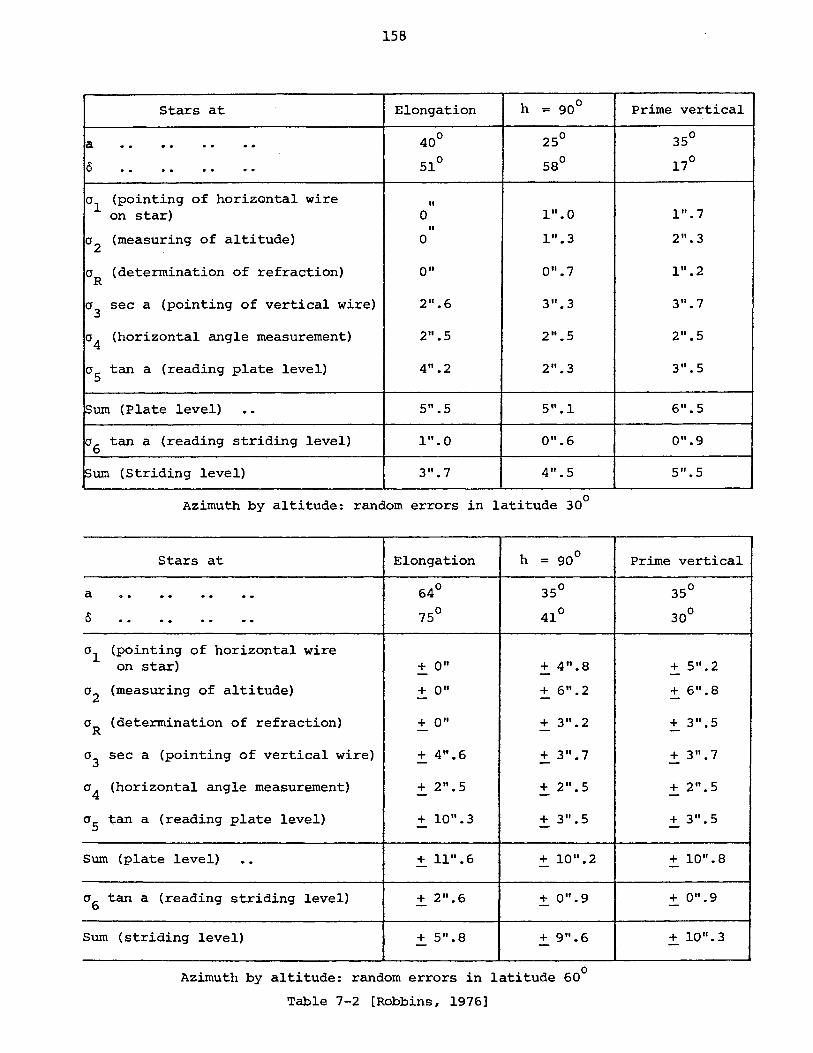
158
Stars at Elongation h = 90°
let · . · . · . · . 40° 25°
0 · . · . · . · . 51° 58°
0'1 (pointing of horizontal wire " on star) 0 1".0 "
0'2 (measuring of altitude) 0 1".3
O'R (determination of refraction) 0" 0".7
0'3 sec a (pointing of vertical wire) 2".6 3".3
0'4 (horizontal angle measurement) 2".5 2".5
0'5 tan a (reading plate level) 4".2 2".3
~um (Plate level) · . 5" • 5 5".1
0'6 tan a (reading striding level) 1".0 0".6
pum (Striding level) 3".7 4".5
Azimuth by altitude: random errors in latitude 30°
a
15
0'1
0'2
O'R
0'3
0'4
0'5
Sum
0'6
Sum
Stars at Elongation h = 90°
· . · . · . · . 64° 35°
· . · . · . · . 75° 41°
(pointing of horizontal wire on star) + 0" + 4".8 - -
(measuring of altitude) + 0" + 6".2 - -(determination of refraction) + 0" + 3".2 - -sec a (pointing of vertical wire) + 4".6 + 3".7 - -(horizontal angle measurement) + 2".5 + 2".5 - -tan a (reading plate level) + 10".3 + 3".5 - -
(plate level) · . + 11".6 + 10".2
tan a (reading striding level) + 2".6 + 0".9 -
(striding level) + 5".8 + 9".6
Azimuth by altitude: random errors in latitude 60°
Table 7-2 [Robbins, 1976]
Prime vertical
35°
17°
1".7
2".3
1".2
3".7
2".5
3".5
6".5
0".9
5".5
Prime vertical
35°
30°
+ 5".2 -+ 6".8 -+ 3".5 -+ 3".7 -+ 2".5
+ 3".5 -+ 10".8 -+ 0".9 -+ 10".3 -
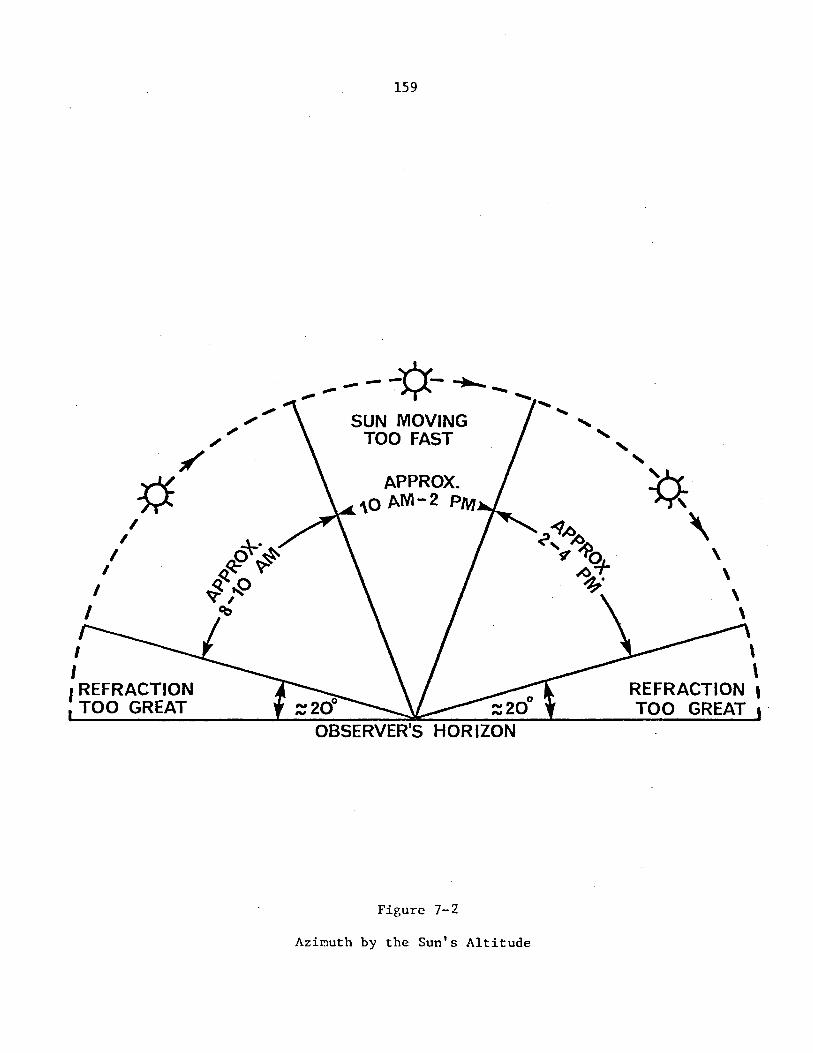
I I , REFRACTION
TOO GREAT
159
__ Yv_~ ."..-"¥ .......
.".. ...... , ..... SUN MOVING "
TOO FAST "
APPROX. ,,0 AM-2 PM
Figure 7-2
Azi~uth by the Sun's Altitude
, , ~" ,
\ \
REFRACTION , TOO GREAT "
is:
160
(iv) Reverse on R.O., record H.C.R., record level readings,
(v) Record temperature and pressure.
The computation procedure resulting from the above observations
(i) Mean Direct and Reverse horizontal readings to the R.O. and to the
Sun,
(ii) correct the horizontal directions in (i) for horizontal axis
dislevelment using equation (7-7),
(iii) compute the angle Sun to R.O.,
(iv) mean direct and reverse zenith distance (or altitude) measurements
to the Sun, then correct the mean for refraction and parallax,
(v) determine the time of observation in the time system required to
obtain a tabulated value of 15 of the sun,
(vi) compute the updated value of 0 for the time of observation
(tabulated 0 plus some correction for time),
(vii) using either (7-13) or (7-14), compute the azimuth to the sun,
(viii) using the angle determined in (iii), co~pute the azimuth to the
R.O.
The following example illustrates the observing and computation
procedures for an azimuth determination via the altitude of the sun.
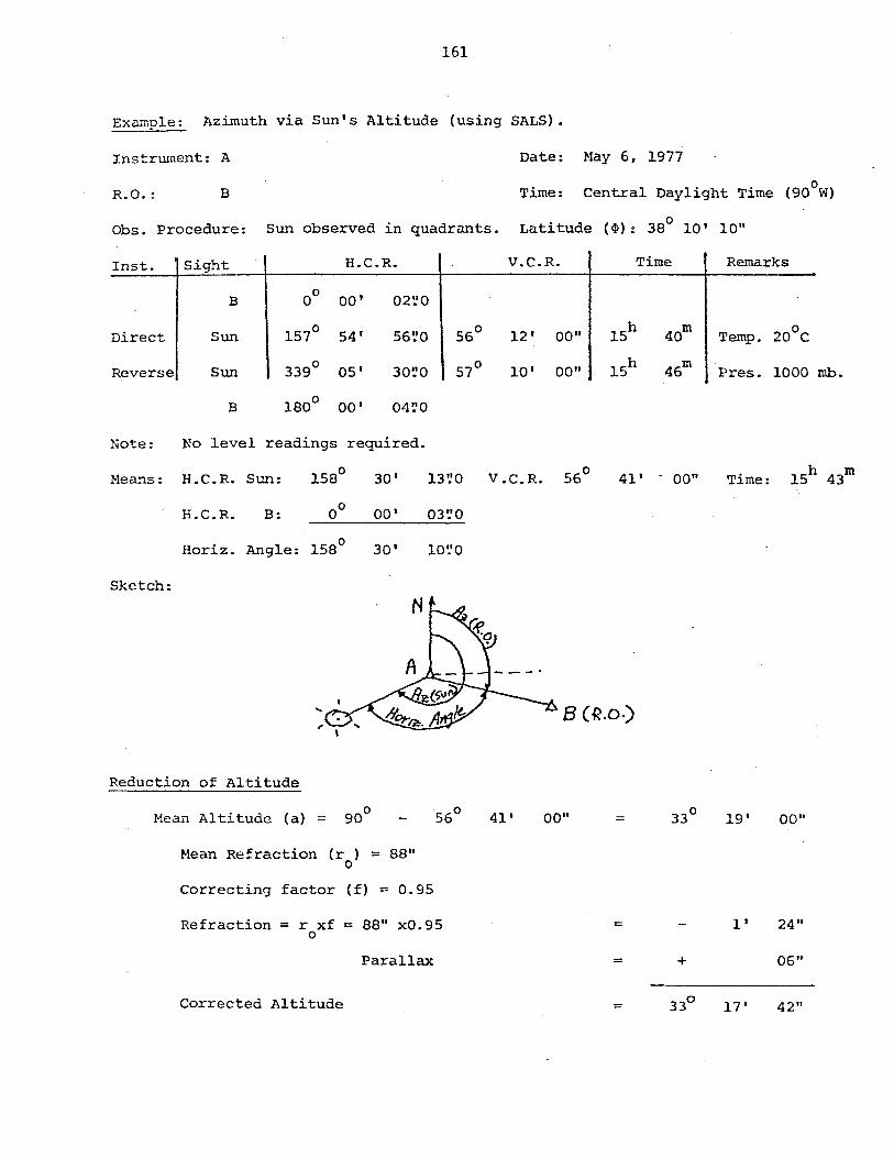
161
Ex~~ple: Azimuth via Sun's Altitude (using SALS).
Instrument: A Date: May 6, 1977
R.O.: B Time: Central Daylight Time (900 W)
Obs. Procedure: Sun observed in quadrants. Latitude (~): 38° 10' 10"
Inst. Sight H.C.R. V.C.R. Time
B 0° 00' 02~0
Direct Sun 157° 54' 56~0 56° 12' 00" ISh 40m
Reverse Sun 339° 05' 30~0 57° 10' 00" ISh 46m
B 180° DO' 04~0
Note: No level readings required.
Means: H.C.R. Sun: 30' l3~0 V.C.R. 56° 41' . 00"
.Sketch:
H.C.R. B:
° Horiz. Angle: 158
Reduction of Altitude
DO' 03~0
30' 10~0
Mean Altitude (a) = 90° S6°
l-1ean Refraction (r ) = 88" °
Correcting factor ( f) = 0.95
Refraction == r xf == 88" xO.95 °
Parallax
Corrected Altitude
8 (R.O.)
41' 00" = 33°
==
= +
= 33°
Remarks
Temp. 20°C
Pres. 1000 mh.
19' ~O''
l' 24"
06"
17' 42"
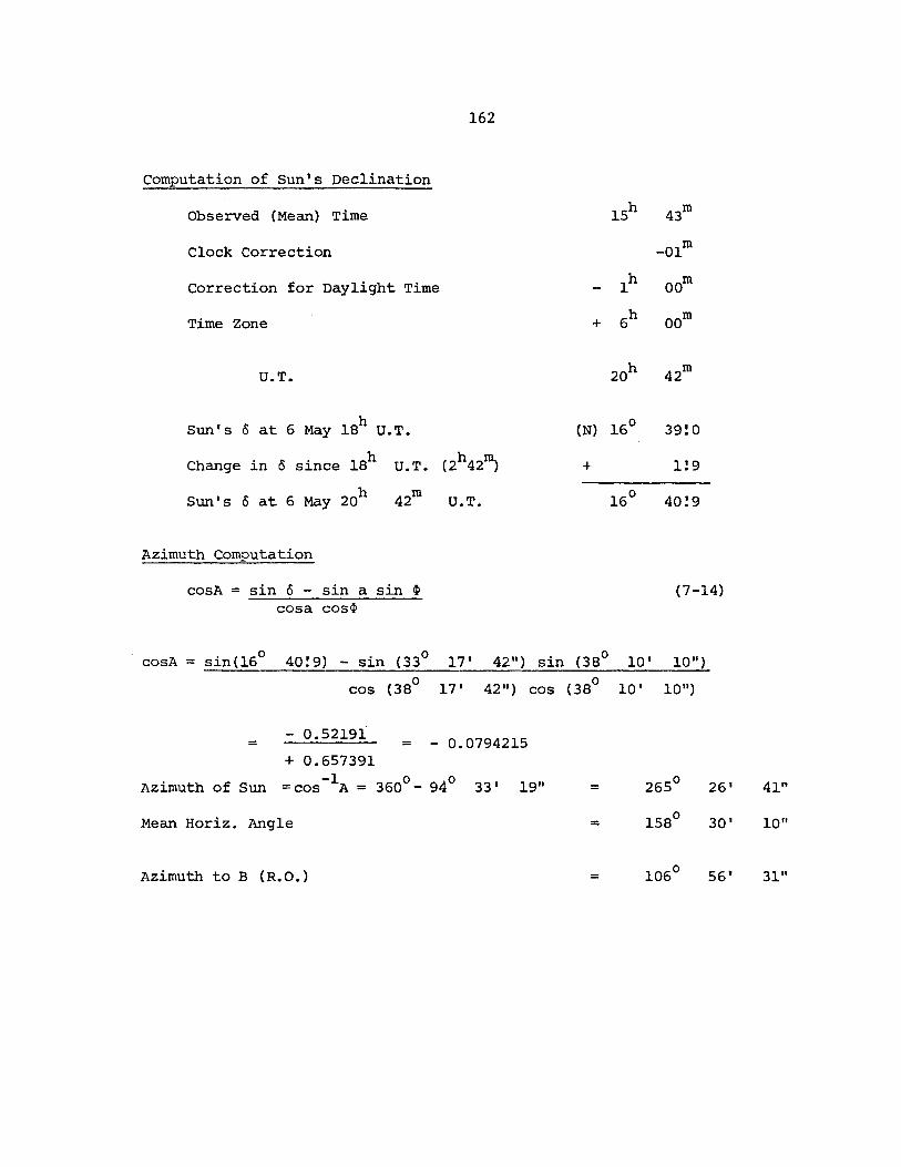
162
computation of Sun's Declination
Observed (Mean) Time
Clock Correction
Correction for Daylight Time
Time Zone
U.T.
Sun's 0 at 6 May 18h U.T.
Change in 0 since 18h U.T. (2h42m)
Sun's 0 at 6 May 20h
Azimuth Computation
cosA
cosA = sin 0 - sin a sin ~ cos a cos~
= sin(16° 40!9) - sin (330
cos (380
- 0.52191 = =
+ 0.657391
U.T.
17' 42")
17' 42")
- 0.0794215
sin
cos
Azimuth of Sun -1 =cos A = 360°- 94° 33' 19"
Mean Horiz. Angle
Azimuth to B (R.O.)
15h 43m
_Olm
III OOm
+ 6h OOm
20h 42m
(N) 16° 39~0
+ 1!9
16° 40!9
(7-14)
(380 10' 10")
(380 10' 10")
= 2650 26' 41"
= 1580 30' 10"
= 106° 56' 31"
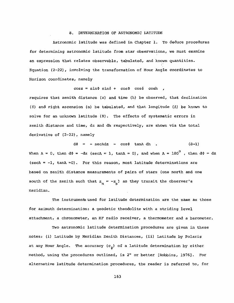
8. DETERMINATION OF ASTRONOMIC LATITUDE
Astronomic latitude was defined in Chapter 1. To deduce procedures
for determining astronomic latitude from star observations, we must examine
an expression that relates observable, tabulated, and known quantities.
Equation (2-22), involving the transformation of Hour Angle coordinates to
Horizon coordinates, namely
cosz = sin~ sino + cos~ coso cosh ,
requires that zenith distance (z) and time (h) be observed, that declination
(0) and right ascension (a) be tabulated, and that longitude (A) be known to
solve for an unknown latitude (~). The effects of systematic errors in
zenith distance and time, dz and dh'respectively, are shown via the total
derivative of (2-22), namely
d~ = - secAdz cos~ tanA dh (8-1)
o When A = 0, then d~ = -dz (secA = 1, tanA = 0), and when A = 180 , then d~ = dz
(secA = -1, tanA =0). For this reason, most latitude determinations are
based on zenith distance measurements of pairs of stars (one north and one
south of the zenith such that zn = -z~) as they transit the observer's s
meridian.
The instrumen~used for latitude determination are the same as those
for azimuth determination: a geodetic theodolite with a striding level
attachment, a chronometer, an HF radio receiver, a thermometer and a barometer.
Two astronomic latitude determination procedures are given in these
notes: (i) Latitude by Meridian Zenith Distances, (ii) Latitude by Polaris
at any Hour Angle. The accuracy (o~) of a latitude determination by either
method, using the procedures outlined, is 2" or better [Robbins, 1976]. For
alternative latitude determination procedures, the reader is referred to, for
163
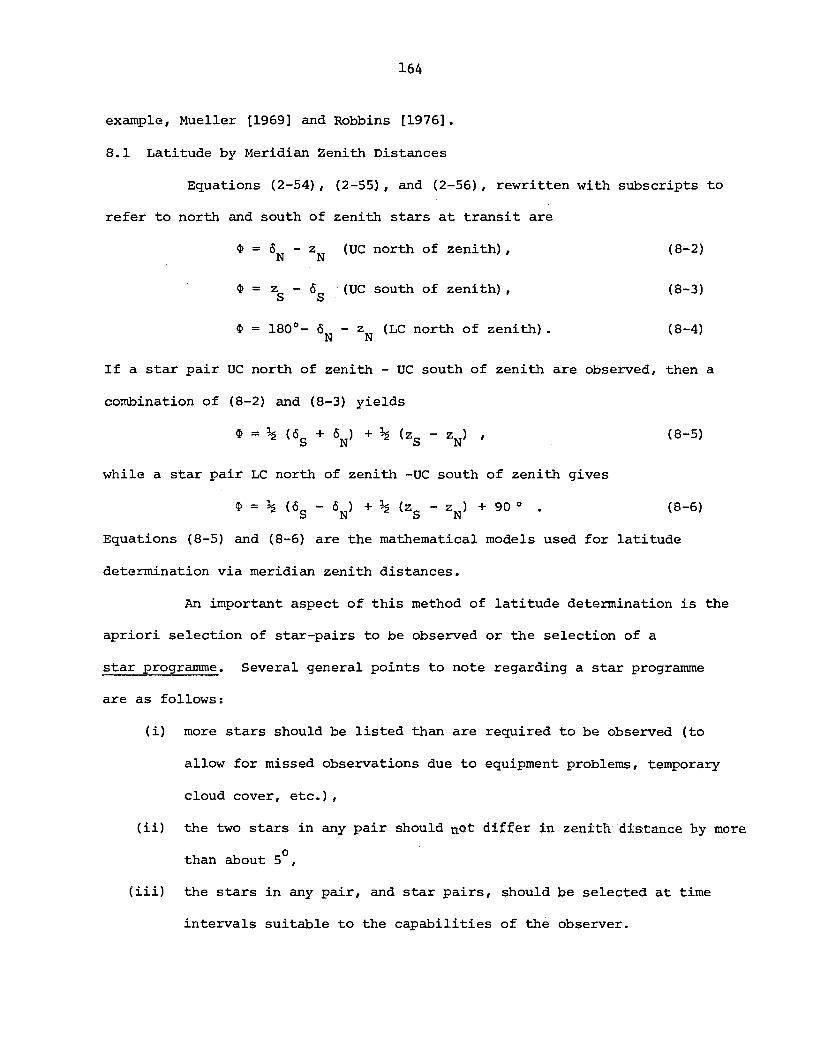
164
example, Mueller [1969] and Robbins [1976].
8.1 Latitude by Meridian Zenith Distances
Equations (2-54)., (2-55), and (2-56), rewritten with subscripts to
refer to north and south of zenith stars at transit are
~ = 5N - z N (UC north of zenith) , (8-2)
~ = z -S 5s (UC south of zenith) , (8-3)
~ = 1800 - 5 - z (LC north of zenith). N N (8-4)
If a star pair UC north of zenith - UC south of zenith are observed, then a
combination of (8-2) and (8-3) yields
(8-5)
while a star pair LC north of zenith -UC south of zenith gives
~ = ~ (5 - 15 ) + ~ (z - z ) + 90 0 S N S N
(8-6)
Equations (8-5) and (8-6) are the mathematical models used for latitude
determination via meridian zenith distances.
An important aspect of this method of latitude determination is the
apriori selection of star-pairs to be observed or the selection of a
star programme. Several general points to note regarding a star programme
are as follows:
(i) more stars should be listed than are required to be observed (to
allow for missed observations due to equipment problems, temporary
cloud cover, etc.),
(ii) the two stars in any pair should not di~fer in zenith. distance by more
o than about 5 ,
(iii) the stars in any pair, and star pairs, should be selected at time
intervals suitable to the capabilities of the observer.
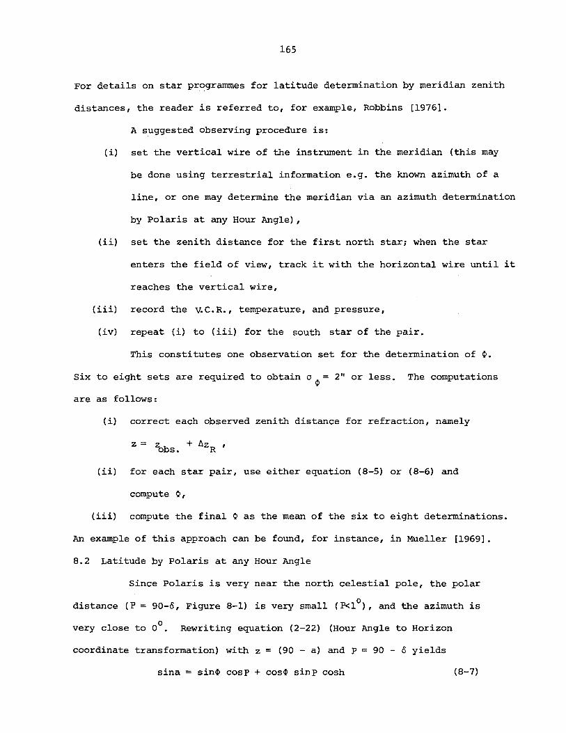
165
For details on star programmes for latitude determination by meridian zenith
distances, the reader is referred to, for example, Robbins [1976].
A suggested observing procedure is:
(i) set the vertical wire of the instrument in the meridian (this may
be done using terrestrial information e.g. the known azimuth of a
line, or one may determine the meridian via an azimuth determination
by Polaris at any Hour Angle),
(ii) set the zenith distance for the first north star; when the star
enters the field of view, track it with the horizontal wire until it
reaches the vertical wire,
(iii) record the V.C.R., temperature, and pressure,
(iv) repeat (i) to (iii) for the south star of the pair.
This constitutes one observation set for the determination of ~.
Six to eight sets are required to obtain (J 4> = 2" or less. The computations
are as follows:
(i) correct each observed zenith distance for refraction, namely
(ii) for each star pair, use either equation (8-5) or (8-6) and
compute ~,
(iii) compute the final ~ as the mean of the six to eight determinations.
An example of this approach can be found, for instance, in Mueller [1969].
8.2 Latitude by Polaris at any Hour Angle
Since Polaris is very near the north celestial pole, the polar
distance (P = 90-~, Figure 8-1) is very small (P<lo), and the azimuth is
° very close to O. Rewriting equation (2-22) (Hour Angle to Horizon
coordinate transformation) with z = (90 - a) and P = 90 - ~ yields
sina = sin~ cosp + cos~ sinp cosh (8-7)
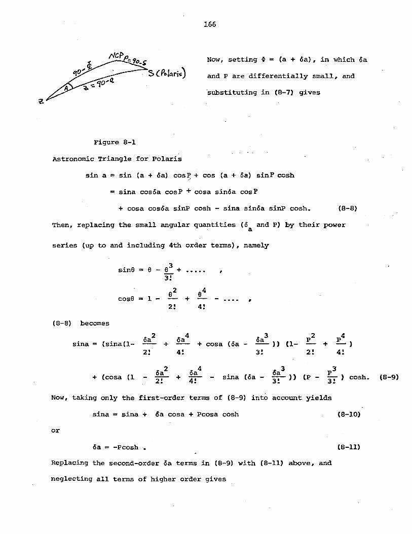
166
Now, setting ~ = (a + ~a), in which oa
and P are differentially small, and
'substituting in (8-7) gives
Figure 8-1
Astronomic Triangle for Polaris
sin a = sin (a + c5a) cosP + cos (a + oa) sinP cosh .'
= sina cosoa cos.P + cosa sinc5a cos P
+ cosa cosoa sinP cosh - sina sin6a sinP cosh. (8-8)
Then, replacing the small angular quantities (6 and P) by their power . a
series (up .to and including 4th order terms), namely
sine = e _e 3 + ..... , 3:
cose 1 -62
+ 64 = - - ,
2: 4:
(8-8) becomes
sina = (sina(l- + . 3 p2
+ cosa (oa - oa » (1- + 2! 4! 3! 2!
+ (cosa (1 3 p3
sina (oa - ~~ » (P - 3: ) cosh. (8-9)
Now, taking only the first-order terms of (8-9) into account yields
sina = sina + oa cosa + Pcosa cosh (8-10)
or
c5a = -Pcosh .• (8-11)
Replacing the second-order c5a terms in (8-9) with (8-11) above, and
neglecting all terms of higher order gives
oa = - Pcosh +
167
. 2h tana sJ.n (8-l2)
Repeating the above process for third and fourth order terms yields the final
equation
~ = a + oa = a - Pcosh +
P . 2 h' 2h 3 sJ.n P cos sJ.n +
P sinP tana sin2h 2
P . 3 . 4h 3 8 sJ.n P sJ.n tan a
(8-l3)
Except in very high latitudes, the series (8-13) may be truncated at the
third term.
A suggested observation procedure is as follows:
(i) observe polaris (horizontal wire) and record V.C.R., time,
temperature and pressure; repeat this three times.
(ii) reverse the telescope and repeat (i).
This constitutes the observations for one latitude determination.
It should be noted that if azimuth is to be determined simultaneously
(using Polaris at any hour angle), then the appropriate H.C.R.ts must be
recorded (such a programme requires that the observer place Polaris at the
intersection of the horizontal and vertical wires of the telescope).
The computation of latitude proceeds as follows:
(i) compute mean zenith distance measurement for six measurements,
(ii) correct mean zenith distance for refraction and compute the mean
altitude (a = 90 - z),
(iii) compute the mean time for a, then using (7-2), compute the mean
h (note that mean a and (a - 12h) must be computed for this part m
of the latitude determination),
168
(iv) compute a mean ~, then P = 90 - 0
(v) compute Ip
A mean of 12 to 20 determinations will yield an astronomic latitude
with alp = 2" or less [Robbins, 1976].
The reader should note that the use of a special SALS table (Pole
Star Tables) leads to a simple computation of latitude using this method,
namely
(8-14)
in which a is the corrected, meaned altitude, and a o ' aI' a2 are tabulated
values. Using this approach results will not normally differ from those using
(8-13) by more than O,:~'2 (12"), while in most cases the difference is within
O!l (6") [Robbins, 1976]. Both computation procedures are illustrated in the
following example taken from Robbins [1976].
Example: Latitude from Observations of Polaris at any Hour Angle
(i) with SALS tables
Date: 23 August 1969
cj>=57003'
A.= 7° 27' W = - Oh 29m 48s
Mean of Observations: a = 56° 57' 24"
Computations:
h RCa -12 +Eq.E) m
Press. = 1009mb.
=
169
GAST :::::: UT + R + R "" 20h 09m 45~4
A oh 29m 485
LAST 19h 39m 57~4
a :::: 56° 57' 24"
" r (mean refraction) :::: 38 °
f (refraction factor) ::::: 1.00
a :::::: a - (r x f) == 56° 56' 46" corr 0
~ == a + a + a l + a 2 == 56° 56 1 46" + 5'48" + 09" corr 0
~ :::: 57 ° 02' 43"
(if) with equation (8-13) (first three terms only)
as in (i) plus:
(l == 2h 03m 095
a.
a ::::: 56° 56'
p ::::: 3163"
4? _. 56° 56' 46 11
46"
+
17"
319~5 + 36~9
~ = 57° 02' 42~'4
+ 00"
9. DETERMINATION OF ASTRONOMIC LONGITUDE
In chapter 3, we saw that l~ngitude is related directly with sidereal
time, namely (egn. 3-3 )
A = LAST - GAST (9-l)
From the Hour Angle - Right Ascension systems coordinate transformations
(egn. 2-31)
LAST = a + h • (9-2)
Replacing LAST in (9-l) with (9-2) yields the expression
A = a + h - GAST (9-3)
This equation (9-3) is the basic relationship used to determine astronomic
longitude via star observations. The right ascension (a) is catalogued, and
the hour angle (h) and GAST are determined respectively via direction and time
observations.
Let us first examine the determination of GAST. Setting TM as the
observed chronometer time (say UTC), and 6T as the total chronometer
correction, then
GAST = TM + 6T
The total correction (6T) consists of the following:
(i) the epoch difference 6T at the time of synchronization of o
UTC and TM times,
(ii) chronometer drift 61T,
(iii) DUTl, given by DUTl = UTl - UTC (see Chapter 4),
(9-4)
(iv) the difference between UTl and GAST at the epoch of observation
given by
LMST
LAST
h = MT + (aM - 12 )
= LMST + Eq.E.
Finally, equation (9-3) reads
A = a + h - (TM + 6T)
170
(9-5)
171
The determination of the hour angle (h) is dependent on the
astronomic observations made. From the Hour Angle - Horizon systems
coordinate transformation (eqn. 2-22),
cosh = cosz - sino sin~
coso cos~ (9-6)
can be used for the determination of a star's hour angle. Now, taking z
and TM as the observed quantities, ~ as a known quantity, and 0 as
catalogued, the sources of systematic errors affecting longitude determination
will be in zenith distance (dz), the assumed latitude (d~), the observed
time (TM) and the chronometer correction (d6T). Replacing h in (9-5) by
(9-6), and taking the total derivative yields
dA = - (sec~ cotA d~ + sec~ cosecAdz + dT + d6T) • (9-7)
Examining (9-7), it is obvious that the errors dT and d6T contribute directly
to dA and can not be elliminated by virtue of some star selections. On the
other hand, d~ and dz can be treated as follows:
(i) when the observed star is on the prime vertical
o 0 (A = 90 or 270 ) , then d~ = 0
(ii) the effects of dz can be elliminated by observing pairs of stars
such that zl=z2 •
As with azimuth and latitude determination procedures in which pairs of stars
have to be observed under certain conditions, a star program (observing
list) must be compiled prior to making observations. For details, the
reader is referred, for example, to Mueller [1969] and Robbins [1976].
The primary equipment requirements for second-order (0). = 3" or
less) longitude determination are a geodetic theodolite, a good mechanical
or quartz chronometer, an HF radio receiver, and a chronograph equipped with
a hand tappet.
172
Finally, before describing a longitude determination procedure, the
reader should note the following. Since the GAST used is free from polar
motion, LAST must be freed from polar motion effects. This is accomplished
by adding a polar motion correction (6A : see Chapter 6) to the final p
determined longitude (not each observation), such that the final form of
equation (9-5) becomes
A = a + h + 6Ap - (TM + 6T)
9.1 Longitude by Meridian Transit Times
(9-8)
When a star transits the meridian, h = oh (or l2h) and a = LAST.
If pairs of stars are observed such that zl = z2' then the effects of dz in
(9-7) are e11iminated. The observation of time (TM) as a star transits the
meridian enables longitude computation using (9-8). The main sources of
error will be d~ and the observation of the stars transit of the meridian
(due partly to inaccurate meridian setting and partly to col1iIiiation). The "
latter errors cause .. :. a timing error. A correction for this effect is computed
from [Mueller, 1969]
dA 15 cosec z = cos db sin z
or db= cos '8 -dA
where dA is the rate for the
yielding db in seconds.
Example
For dA = I' = 4s
s dbN = 5.85
star to travel I'
db = 0~80. s
(9-9)
(9-10)
(4s ) of arc in azimuth,
Then, if the longitude difference determined from north and south stars is
s 2.0, the corrections to A are as follows:
(2.0 x 5.85)
5.85 + 0.80 =
173
A (2.0 x 0.80) s 4 dlL = --.!.=-:..::.....;:;;:.....;:;..;;....::.=..!- = 0 • 2 s
(5.85 + 0.80)
A suggested field observation procedure for the determination of
longitude by meridian transit times is [Mueller, 1969]:
(i) make radio-chronometer comparisons before, during, and after each
set of observations on a star pair,
(ii) set the instrument (vertical wire) in the meridian for the north
star and set the zenith distance for the star; when the star
enters the field of view, track it until it coincides with the
vertical wire and record the time (hand tappet is pressed),
(iii) set the instrument for the south star of the pair (do not
reverse the instrumen~ and repeat (ii),
(iv) repeat (ii) and (iii) for 12-16 pairs of stars.
The associated computation procedure is as follows:
(i) compute the corrected time for each observed transit (e.g. TM + ~T) ,
(ii) compute the apparent right ascension for each transit,
(iii) compute the longitude for each meridian transit using (9-8),
(iv) compute dh for each star; compute .hA ~ AN-As for each star pair;
(v)
(vi)
11.2] •
compute the correction to longitude (dIl) for each star of a pair
(see example),
compute the mean longitude from the 12-16 pairs,
apply the correction hA to get the final value of longitude. p
An example of this procedure is given in Mueller [1969; Example
174
In closing, the reader should be aware that there are several other
methods for second order longitude determination. For complete coverage of
this topic, the reader is referred to Mueller [1969) and Robbins (1976).
175
REFERENCES
Astronomisches Rechen-Institut, Heidelbe,rg [1979]. A,Eparent Places of Fundamental~ta~s',l,981 : Containing 'the-:1535 "Sta~$':"irt;,tbe: Fourth FtiIidame,tibil ;Catalogue~', (APFS) ~ 'Ver1agG~ Braun; ;Kar1sruhe.
Boss, B. [1937]. General Catalogue of 33342 stars for the epoch 1950.0, (GC). publications of the Carnegie Institute of Washington, 468. Reissued by Johnson Reprint Co., New York.
Eichorn, 'H. [1974]. Astronomy of Star Positions. Frederick Ungar Publishing Co., New York.
Fricke, W. and A. Kopff [1963]. Fourth Fundamental catalogue resulting from the revision of the Third Fundamental Catalogue (FK3) carried out under the supervision of W. Fricke and A. Kopff in collaboration with W. Gliese, F. Gondolatsch, T. Lederke, H. 'Nowacki, W. Strobel and P. Stumpff, (FK4). Veroeffentlichungen des Astronomischen ReckenInstituts, Heidelberg, 10.
H.M. Nautical Almanac Office [lg8~]. The star Almanac for Land Surveyors for the year 1981. Her Majesty's Stationery Office, London. (in Canada: Pendragon House Ltd. 2525 Dunwin Drive, Mississauga, Ontario', L5L 1T2.)
Heiskanen, W.A. and H. Moritz [1967]. Physical Geodesy. W.H. Freeman and Company, San Francisco.
Krakiwsky, E.J. and D.E. Wells [1971]. Coordinate Systems in Geodesy. Department of Surveying Engineering Lecture Notes No. 16, University of New Brunswick, Fredericton.
Morgan, H.R. [1952]. Catalog of 5268 Standard Stars, 1950.0. Based on the Norman System N30. Astronomical Papers Prepared for the Use of the American Ephemeris and Nautical Almanac, 13, part 3. Government Printing Office, Washington, D.C.
Morris, William (editor) [1975]. The Heritage Illustrated Dictionary of the English Language. American Heritage Publishing Co., Inc.
Mueller, Ivan I. [1969]. Spherical and Practical Astronomy as Applied to Geodesy. Frederick Ungar Publishing Co., New York.
Robbins, A.R. [1976]. Military Engineering, Volume XIII-Part IX, Field and Geodetic Astronomy. School of Military Survey, Hermitage, Newbury, Berkshire, U.K.
Roelofs, R._[1950]. Astronomy Applied to Land Surveying. N.V. Wed. J. Ahrend & Zoon, Amsterdam.
U.S. Naval Observatory, Nautical Almanac Office [19'801. The Astronomical Almanac fo"'( the Year 19.81; U.S'.' Governm~nt P"'(intina Offi~, Washington,
, D.C.
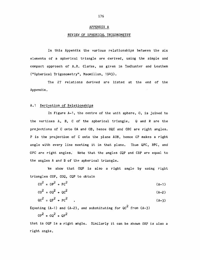
176
APPENDIX A
REVIEW OF SPHERICAL TRIGONOMETRY
In this Appendix the various relationships between the six
elements of a spherical triangle are derived, using the simple and
compact approach of A.R. Clarke, as given in Todhunter and Leathem
("Spherical Trigonometrytt, Macmillan, 1943).
The 27 relations derived are listed at the end of the
Appendix •
A.1 Derivation of Relationships
In Figure A-l, the centre of the unit sphere, 0, is joined to
the vertices A, B, C of the spherical triangle. Q and R are the
projections of C onto OA and OB, hence OQC and ORC are right angles.
P is the projection of C onto the plane AOB, hence CP makes a right
angle with every line meeting it in that plane. Thus QPC, RPC, and
OPC are right angles. Note that the angles CQP and CRP are equal to
the angles A and B of the spherical triangle.
We show that OQP is also a right angle by using right
triangles COP, COQ, CQP to obtain
C02 = Op2 + PC2
C02 = OQ2 + QC2
QC2 = Qp2 + PC2
Equating (A-l) and (A-2), and substituting for QC2 from (A-3)
Op2 = OQ2 + Qp2
(A-1)
(A-2)
(A-3)
that is OQP is a right angle. Similarly it can be shown ORP is also a
right angle.
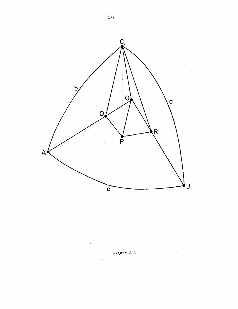
177
c
A
_____ ----8
Figure A-1
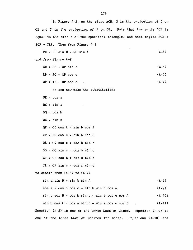
178
In Figure A-2, on the plane AOB, S is the projection of Q on
OB and T is the projection of R on OA. Note that the angle AOB is
equal to the side c of the spherical triangle, and that angles AOB =
SQP = TRP. Then from Figure A-1
PC = RC sin B = QC sin A (A-4)
and from Figure A-2
OR = OS + QP sin c
RP = SQ - QP cos c
QP = TR - RP cos c
We can now make the substitutions
OR = cos a
RC = sin a
OQ = cos b
QC = sin b
QP = QC cos A = sin b cos A
RP = RC cos B = sin a cos B
OS = OQ cos c = cos b cos c
SQ = OQ sin c = cos b sin c
OT = OR cos c = cos a cos c
TR = OR sin c = cos a sin c
to obtain from (A-4) to (A-7)
sin a sin B = sin b sin A
cos a = cos b cos c + sin b sin c cos A
sin a cos B = cos b sin c - sin b cos c cos A
sin b cos A = cos a sin c - sin a cos c cos B
(A-5)
(A-6)
(A-7)
(A-8)
(A-9)
(A-10)
(A-11 )
Equation (A-8) is one of the three Laws of Sines. Equation (A-9) is
one of the three Laws of Cosines for Sides. Equations (A-lO) and
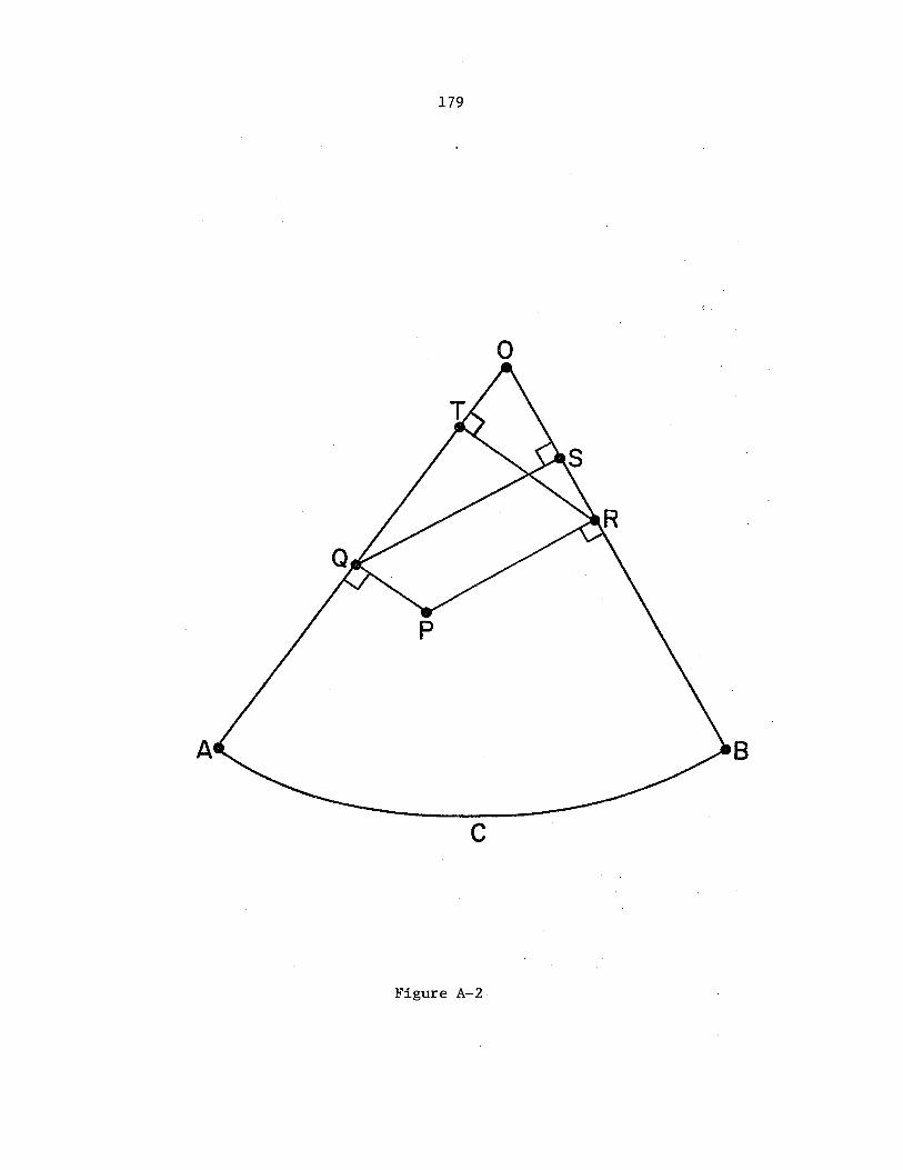
179
o
8
c
Figure A-2
180
(A-11) are two of the twelve Five-Element Formulae.
The Four-Element Formulae can be derived by multiplying
Equation (A-10) by sin A, and dividing it by Equation (A-8) to obtain
sin A cot B = sin c cot b - cos A cos c
rearranged as
cos A cos c = sin c cot b - sin A cot B (A-12)
Similarly multiplying Equation (A-11) by sin B and dividing by the
transposed Equation (A-B) we obtain
cos B cos c = sin c cot a - sin B cot A (A-13)
Equations (A-12) and (A-13) are two of the six Four-Element Formulae.
It can be shown that all the above Laws remain true when the
angles are changed into the supplements of the corresponding sides and
the sides into the supplements of the corresponding angles. Applying
this to Equations (A-8) , (A-12), and (A-13) will not generate new
equations. However, when applied to Equation (A-9)
cos a = cos b cos c + sin b sin c cos A
it becomes
cos(n-A) = cos(n-B)cos(n-C)+sin(n-B)sin(n-C)cos(n-a)
or
cos A = - cos B cos C + sin B sin C cos a
which is one of the three Laws of Cosines for Angles.
Equations (A-l0) and (A-ll) become
sin A cos b = cos B sin C + sin B cos C cos a
sin B cos a = cos A sin C + sin A cos C cos b
which are two more of the twelve Five-Element Formulae.
(A-14)
Similarly
(A-15)
(A-16)
Equations (A-8) to (A-16) represent one-third of the
relationships. The other two-thirds are obtained by simultaneous
181
cyclic permutation of a, b, c and A, Bt C. For example. from Equation
(A-B)
sin a sin B = sin b sin A
we obtain
sin b sin C = sin c sin B
sin c sin A = sin a sin C
The entire set of 27 relations obtained this way are stated below.
A.2 Summary of Relationships
A.2.1 Law of Sines
sin a sin B = sin b sin A
sin b sin C = sin c sin B
sin c sin A = sin a sin C
A.2.2 Law of Cosines (sides)
cos a = cos b cos c + sin b sin c cos A
cos b = cos c cos a + sin c sin a cos B
cos c = cos a cos b + sin a sin b cos C
A.2.3 Law of Cosines (angles)
cos A = - cos B cos C + sin B sin C cos a
cos B = - cos C cos A + sin C sin A cos b
cos C = - cos A cos B + sin A sin B cos c
A.2.4 Four-Element Formulae
cos A cos c = sin c cot b - sin A cot B
cos B cos a = sin a cot c - sin B cot C
cos C cos b = sin b cot a - sin C cot A
cos B cos c = sin c cot a - sin B cot A
A.2.5
182
cos C cos a = sin a cot b sin C cot B
cos A cos b = sin b cot c - sin A cot C
Five-Element Formulae
sin a cos B = cos b sin c - sin b cos c cos A
sin b cos C = cos c sin a - sin c cos a cos B
sin c cos A = cos a sin b sin a cos b cos C
sin b cos A = cos a sin c - sin a cos c cos B
sin c cos B = cos b sin a - sin b cos a cos C
sin a cos C = cos c sin b sin c cos b cos A
sin A cos b = cos B sin C + sin B cos C cos a
sin B cos c = cos C sin A + sin C cos A cos b
sin C cos a = cos A sin B + sin A cos B cos c
sin B cos a = cos A sin C + sin A cos C cos b
sin C cos b = cos B sin A + sin B cos A cos c
sin A cos c = cos C sin B + sin C cos B cos a
110 I
183
APPENDIX B
CANADIAN TIME ZONES
/ I I I'J 120
100 I
(Canada Year Book 1978-79, Dept. of Supply and Services, Ottawa)
No. I US3
125-1
uS5
368
370
1256
371
373
1257
372
374
375
377
376
378
1258
1259
1200
1261
·379
380
:;81
:;85
382
3~4
383
:262
I~G.l
uli4
uGS
I
184
APPENDIX C
EXCERPT FROM THE FOURTH FUNDAMENTAL CATALOGUE (FK4)
EQUINOX AND EPOCH 1950.0 AND 1975.0
Name
I "···1 sp. dx d'ct J,.
1-:1"(%) ct dT .~ . .iii " d7'
I
+ 19"2J34 I.co 6.92 Ko rJ'43'" 5!-IH + 333!:41 - O!i09 + o!.60 -O!OOI 2j·H 9 44 28.710 + 332.1>87 - 0.705 + 0.160 -0.001
I Car 3.6 '-1.8 Go 9 -13 52.35-1 + 164.799 - 0.0<J6 - 0·%34 -0.003 10 .. l2 9 ~-I 3J.553 + 164.796 - 0.005 - 0.235 -0.003
Dr 1369 UMa 5. 20 Go 9 45 27.4H + 386.859 - :.201 + l!.l6: -0.0:6 :6.08 9 46 59.02• + 385.701 - 2.190 + 2.156 -0.0:6 .
" U!\la 3.89 Fo + 426.403 - 3·9S5 - 3·817 16,50 9 47 27-'02 +0.032 949 IHH + 42-1.418 - 3-955 - 3.809 +0.033
6Su: 6.00 At. 9 48 42.$:6 + 3°2·309 - 0.118 + 0.057 -0.001 17.29 9 49 58.396 + 302•251 - 0.111 + 0.05i· -0.001
162 G. Vel HZ Ko 9 49 13.441 + 232.';00 + 0.48: - 0.380 -0.001 21 .. $3 9 So 21·571 + 232•643 + 0.490 - 0.380 -0.001
/l Leo 4·10 Ko 9 49 55·434 + 341.140 - 0·969 - 1·599 +0.004 1-1·55 9 51 20.659 + ]40.657 - 0.963 - 1·591$ +0.00-1
183 G. Hya 5.16 lIo 9 52 30.60: + 282.989 + 0.168 - 0.358 -0.003 19.27 9 53 41.360 + 283.075 + 0.174 - 0·359 -0.003
1$ G. Sex 7.03 Ko 9 53 38.894 + 298.06: - 0.039 - 0.166 0.000 z6 .. p 9 54 5H07 + 298.043 - 0.035 - 0.166 0.000
Grb 1586 UMa 5.96 Ko 9 53 57.521 . + 535.718 -10.691 - 1·733 +0.031 20·57 9 56 10.786 + 530.415 -10.523 - 1.72 5 +0.032
19 LMi 5·19 FS 9 54 37.760 + 367.318 - 1.767 . - 1.056 +0.006 20.46 9 56 9-479 + 366.437 - J.7S$ - 1.055 +0.006
'1' Vel 3·70 B5 9 55 6.~49 + zlo·696 + 0.487 - O.I]~ -0.001 13-38 9 55 58.954 + 210·9~1 + 0.495 - 0.13$ -0.001
11 Ant 5·=5 Fo 9 56 43-347 + 257·';'9 + 0.438 - 0.806 -0.006 18.47 9 57 47.729 + 257.6]9 + 0·445 - 0.808 -0.006
u Sex 6.63 A5 9 57 7·479 + 311•188 - 0.276 - 0.-163 +0.001 u·33 9 58 25.259 + 3".051 - 0.271 - 0..;63 oj·O.OOI
:r L~o 4-89 Mo 9 57 34·334 + 317.018 - 0·393 - 0.21 5 -0.001 13.03 9 58 53.564 + :;16.823 - 0.389 .- 0.21 5 -0.001
20 I.,.:i 5.60 GS 9 58 8.'.115 + .H5·802 '- 1.230 - 4·14.0 '40.006 24·37 9593H89 + 345.11>9 - 1.223 - 4·139 +0.006
Pi 9h229 UM,. 5·74 FS 10 I 17·747 + 398.561 - 3.066 - 0.269 +0.003 36.41 10 2 57.196 + 397·034 - 3.044 - 0.26S +0.003
193 G. Hya 5·80 Fo 10 2 2.261 + 277.137 + 0.:8$ - 0.845 -0.002 19.07 10 3 11.563 + 277.283 + 0.29-1 - 0.846 -0.003
,,' Hy3 4·72 D8 10 :: 41.299 + 292•143 + 0.086 - 0.289 0.000 12.88 :0 :; 54.340 + 292.IS7 + 0·09-' - 0.259 0.000
11 Leo 3.58 Aop 10 4 36.533 + 327.034 - 0.637 - o.OIZ 0.000 16.51 10 S 58•252 + 326.71; - 0.6]2 - 0.0:2 0.000
IE Leo 1·34 D8 10 S 42.647 + 319.462 - 0.489 - 1.6g6 +0.003 08.Sz 10 7 2·482 + 319.219 - 0 ... 8 .. - 1.695 +0.00]
1. lIya 3·S3 Ko 10 S 8.945 + 292.48, + 0.080 - 1.';07 -0.006 15·45 10 9 22.070 + 292.5:: ·t 0.<>S5 - 1.40S -0.006
(Q Car 3.56 118 10 IZ 33.0-17 + 142.7°3 - 0.391 - 0.6:5 -0.014 11.62 10 13 S·t)9S + 142.506 - 0·:;97 - 0;6:9 -0.014
19' G. Vel 4·09 A2 10 I:l 37.998 of· 251.899 + 0.(109 - 1·345 -o.ooS 16·5; 10 '3 41.011 + 2';~.:Ot; + 0.618 - 1·34; -O.OO~
C JeD 3·Gs Fo 10 '] 54.75S + 333.6.: - o.SSS + o.IH -0.001 IS·9i
I 10 IS Ig.107 + 333.184 - 0.852 + 0.134 -0.001
i. \J!\b HZ A: 10 14 ).353 + 361•689 - 1.877 - 1.512 +0.010 IS·9S 10 I:: 3S·"SS + 360.7;'; - I.S04 - 1·509 -10.010
:;2 Ul\b. 5·74 A3 10 14 25.657 + ·435 .. B'; - 5.542 - 1_3S0 +0.024 :13.4 2 10 16 14.171 + H2.080 - 5·475 - 1·3;4 -It'.?:"
e S:>t 5.40 Fo 10 IS 8.659 + 29S.118 + 0.(111 - 1.104 -n.<J?1 17· I g 10 If> 23.1)19 ~. =9S.I:5 ~. 0."11j - 1.1::-'; -,0.0'>1
187 G. C3. 3·44 KS 1<' is 24.581 + :00.367 + o·S~7 - 0·3.3 -0.0.'16 I·P9 10 16 14.il0 + :oo.60~ oj. v.6oS - 0·3.4 -0.006
)'J G •• \ .. t $.(,2
I D!/ 10 15 .19·9'l-'I
I + :;5.0 39 + O~':.!5 - 0.116 0.0<» 19·1>~
10 !6 SS.69S .•. 27).2,)4 + 0·433 - ".IIG 0.000
1>1 (2) r>, (,.)
z.S IS
9·,; -II
:r.~ u
z.6 10
1·4 9
7.6 40
1·4 6
2.1 13
2 .. ; 16
4.6 21
:Z.o 10
5.6 SO
3.6 ZJ
1·9 II
1.2 5
2.5 II
:;·9 19
2·9 IS
1.8 10
1·4 6
1.0 4
I.,: 7
9·:; 49
4·-1 zo
1·4 ,. 1·9 S
4., IS
I., 9
9·! 39
s·.:! IS
I
185
EQUINOX AND EPOCH 1950.0 AND 1975.0
.-li
,111 d:') I"
dl,I EI" (J) 711 ("> ,n (,,') GC N30
dT' ! iii>! 'rii
US3 +JSo 5';' 53~4l - 16SI!!91 -13!JI - l!i6· -0!01 26.00 '4·0 26 Int-!- 2335 +18 47 57.86 -1665·53 -13. 17 - ,.j6 -0.01
-62 16 3" .. ;% -1650.65 - 6.36 + 0·33 +C.02 11.64 5·9 :15 13.162 233'> -62 23 31·9S -1663.82 - 6·33 + 0·33 +0.02
+46 IS 18.ll -1677.S:, -15.36 - 9.53 -0.18 19.20 3.2 12 13';97 :1345 +46 8 li.i2 - 1685.44 -15.14 - 9·S6 -0.17
u.ss
+59 16 30.31 -1693.85 -16 . .;8, - 15-55 +0.30 09·5' 2.2 8 13540 2355 +59 9 25.83 -17°2.02 -16.20 - 15.48 +0·:19
-( o 29.53 -1687·48 -11·59 - 3.18 0.00 17·74 2·4 13 13558 2357 -4 7 32•11 -1693-25 -11·48 - 3.18 0.00
370
-45 57 33·54 -1684·48 - 8·i6 + 3.03 +0.03 20.6') 7.2 40 13574 2362 -46 4 35.21 -1688.s,. - 8.71 + 3.0'; +0.03
+26 14 36•08 -1696.01 -12·94 - 5·99 +0.12 08.03 2.1 8 13590 :l36.; +26 7 31•2 i -17°2·44 -1%·i9 - 5.96 +0.12
371
373 -18 46 18.u -1706.39 -10.51 - 4·22 +0.03 21.81 3.8 21 136.&4 2367 -18 53 25-34 -17".52 -10,42 - 4·21 +0.03
- 7 24 26·90 -17°7.41 -11.01 - 0.11 +0.01 24·43 4·1 26 13674 2371 -7 31 34·44 -1712•89 -10·90 - O.ll "0.01
1257
"73 7 P7 -1712.77 -19·98 - 4.05 +0.13 14-8, 2·5 12 13684 2373 +7:1 59 5i·74 -1722•63 -19·45 - 4·0:1 "0.13
372
"41 17 40.83 -1714.6') -13·5:1 - :1·91 +0.08 16-42 :l·7 lZ 13700 :1376 +41 10 31.32 -1721.40 -13·33 - 2·89 .. 0.08
~j4
-S.J 19 44.86 . -1713.48 - 7·59 + 0.46 +0.01 10.61 4.6 22 13711 237'1 -54 26 53.70 -1717.26 - 7·55 + 0·46 +0.01
375
-35 39 3.66 -1723.64 - 9.21 - 2.41 +0.06 19·37 4-5 :z6 13741 2387 -35 46 15.14 -1728.23 - 9.15 - 2·39 +0.06
377
+ 3 37 28.41 -1721·34 -11.20 + 1.6') +0.03 19.14 3·3 16 13746 2389 + 3 30 Ij·38 -1726.91 -1I.oS + 1·70 +0.03
+8 17 5-76 -1727.67 -11·39 - 2.6.J +0.02 09.71 1·9 7 13755 2390 +8 9 53.13 -1733·33 -1l.26 - :l.64 +0.02
+32 10 13.66 -177°·84 -12.25 - 43.32 +0.32 17-73 3.2 13 13763 :l391 +32 2 50.19 -1776.92 -12·09 - 43.24 +0.32
+54 8 4·53 -1742.04 -14·00 - 0.66 +0.02 26.'7 44 .6 13827 2397 .+54 o 4S.15 -1748.gS -13.76 - 0.66 +0.02
1259
-24 :I 3-\.25 -1742.75 - 9·5-\ + 1.83 +0.06 18.20 4.0 :6 138.;8 '402 -24 9 50·53 -1747·5° - 9.46 + 1.85 +0.06
1260
1261 -12 49 'j·50 -1746.4= -.0.05 + 0·95 +0.0% 12·09 2·7 14 13861 z¥>8 -12 5634-73 -175'.42 - 9·95 + 0.96 +0.02
+17 o 26"7 -1756.12 -11.12 - 0.58 0.00 13.83 :l.2 9 13899 :l41:1 + 16 53 6.45 -176,.65 -10·99 - 0.58 0.00
379
+u 12 44.54 -1759·9' -10·70 + 0.26 +0.12 01·35 ··7 5 13926 24'4 +12 5 23·90 -li65·23 -10·57 + 0.29 +0.12
-12 6 22.55 -1779·73 - 9·57 - 9.46 +0.10 14·0 j :l·3 II 13982 2424 -12 13 48.08 -li8.;·49 - 9·47 -:- 9·44 +0.10
-69 47 :!J·35 -1787-70 - 4.30 + 0.29 +0.04 12·97 4·6 23 14074 2434 -69 54 4"·54 -1789.84 - 4.27 + 0·3° +0.0.0
-41 52 25.23 -1784047 - 7.86 + 3·84 +0·09 14.27 4·7 22 14076 ::1435 -4' 59 51•84 -li88.39 - i.SQ + 3.86 +0·09
+23 40 1-9~ -1794·55 -10.48 - 1.21 -0.01 '5·37 2.2 10 14107 ::144° +%3 32 3~·65 -1799·75 -10·33 .- 1.21 -0.01
+43 953·H -179~29 -11.32 - 4.26 +0.10 06.91 2·4 S 14113 244% +43 2 23.:6 -· ISo3·90 -11.13 - 4.24 +0.10
.:62 +65 %1 31.58 -1;96·54 -13.65 - 1.19 +0·09 13.14 ].0 12 14123 '445 .. 65 14 I.h-;) -IS"3·30 -13-36 - 1.17 +0·09
.. - 7 49 6.;8 -1798.22 - 9.18 - 010 +o.Oj 16.67 2·7 IS '4129 2446 -7 56 36.91 -1~":·iS - 9·07 - o.oS +0,"7
-61 .. 5j·O'\ '-17~~.~t; - 6.04 + o·~9 +o.o~ 13.8., 5·9 :l4 14133 2448 .. 61 I: 25. 1; -11'::>1·:-7 • ... 6.00 + 0.30 ..... O.Ol I -·as H =9·0~ I ~1;9"·92 I - S.41 I 01- 0.8S ·to.OI 19."') 4·5 25 14144 =45° -28 51 39·5·!· ":&-'1. 1 1 ! - S·';3 I + 0.5S ;C.OI I I I
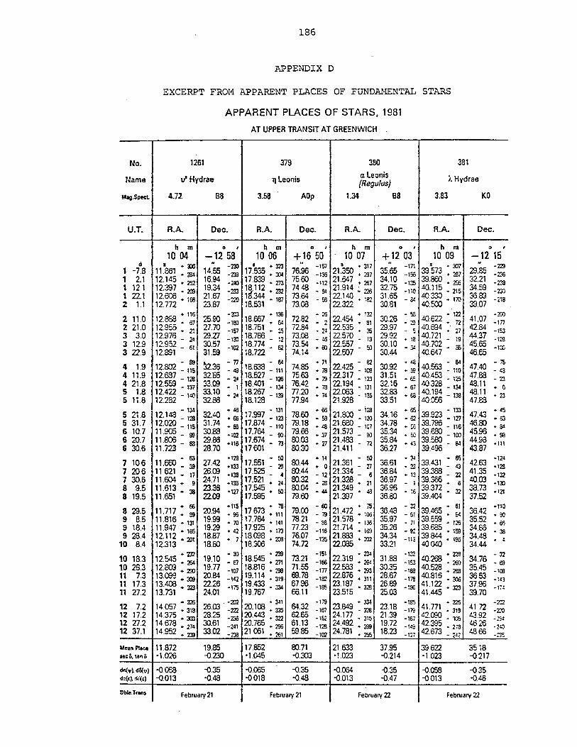
186
APPENDIX D
EXCERPT FROM APPARENT PLACES OF FUNDAMENTAL STARS
APPARENT PLACES OF STARS, 1981
AT UPPER TRANSIT AT GREENWICH
---·--T---------------r--------------.--------------~---------------
No.
Name
Mafl·SpeeL
U.T.
d 1 -7.8 1 2.1 1 12.1 1 22.1 2 1.1
:2. 11.0 2 21.0 3 3.0 3 12.9 3 22.9
4· 1.9 4 11.9 4 21.8 5 1.8 5 11.8
5 21.8 5 31.7 G 10.7 I; 20.7 6 30.6
1 10.6 7 20.6 1 30.6 8 9.5 8 19.5
8 29.5 9 8.5 9 18.4 9 28.4
10 8.4
10 18.3 10 28.3 11 7.3 11 17.3 11 272
1261 379 380 381
" Hydrae Tlleonis IX Leonis (Regulus) i. Hydraa
4.7.2 SS 3.58 AOp 1.34 88 3.83 KO
RA Dec. R.A. Dec. R.A. Dec. RA Dec.
b m 0' h mOl h m 0' h m ", 1004 -1258 10 06 + 16 50 10 01 + 12 03 10 09 -12 15
S + JOO 11.861 .~ 12.145 .. 252 12.397 + 2C9 12.600 .. 166 12.772
.. 116 12.888 .. 67 12.955 • 21 12.976 _ 24 12.952 _ 61 12.001
- 89 12.802 _ 115 12.687 _ 128
12.559 137 12.422 -12.282 - 140
'2.148 - 134 - 128
12.020 _ 115 11.905 _ 99 11.806 _ 83 11.723
- 63 11.660 _ 39 11 621 _ 17 11.604.. 9 11.613 .. 38 11.651
.. 66 11.717 .. 89 11.816 .. 131 11.947 .. 165 12.112 .. :<Dl 12.313
.. Zl2 12.545 + 264 12.809 .. 230 13.COO .. :lOO 13.408 .. 323 13.731
14.55 16.94 19.34 21.67 23.87
25.90 27.70 CJ.27 30.57 31.59
-23) S .. 3Zl -m 17.535 .. 304
-240 -233 -220
-203 -100 -157 -130
17.839 • 273 18.112 + 232 1 S".344 .. 187 18.531
.. 136 18.~7 .. 84 18. i51 .. 35 18.786 18.774 - 12
-102 18.722 - 52
,",,, - n "".36 • 49 32.85 _ 24 33.09 _ 1
33.10 32.86
.. 24
- 64 18.638 _ 111 18.527 _ 126 18.401 _ 134 18.267 _ 139 18.128
32.40 31.74 30.88 29.86 28.70
27.42 26.09 24.71 23.36 22.00
20.94 19.99 19.29 18.87 18.80
+46 .. 66
-as -102 +116
17.997 = :~ 17.874 _ 110 17.764 17.674 - 90 17.601 - 73
+128 - 50 +133 17.551 - 26 .138 17.525 - 4 +135 17.521 ... 24 -127 17.545 .. 50
17.595 +115 .. 78 .. 9S 17.673 .. 111 .. 10 17.784 .. 141 .. 42 17.925 • 173
18.098 .. 2C8 18.306
.. 7
76.96 75.60 74.48 73.64 73.08
72.82 72.84 73.08 73.54 74.14
-157 2'"350 • 317 -136 . • 297 -112 21.647 .267 _ 84 21.914 ~ 226 - 56 22.140 • 182
22.322 - 26 .. 1!2 .. 2 22.454 ... 81 _ 2~ 22.535 .. 35 • .:s 22.570 - 13 .. &l 22.557 - 50
22.507
74.85 : ~ 75.63 + 79 76.42 77.20
·78 .. 74
- 82 22.425 _ 100 22.317 _ 123 22.194 _ 131 22.063 135 21.928 -77.94
78.60 79.18 79.66 80.03 80.30
80.44 80.44 80.32 80.04 79.60
., 66 .• ;28 .. 58 21.800 - 120 .. 48 .21.680 - 107 ... 37 21.573 - 90 • 27 21.483 - 72
21.411 .. 14 21.361 - 50 + 0 - 27 .• 12 21.334 - 6 - 28 21.328 .. 21 - 44 21.349 .. 48
21.397
35.65 34.10 32.75 31.65 30.81
30.26 29.97 29.92 30.10 30.44
30.92 31.51 32.16 32.83 33.51
34.16 34.78 35.34 35.84 36.27
-171 S - :m -155 39.573 237 -135 39.800 : eli -110 40.115 • 215 _ 64 40.330 • 170
4O.ECO '" -- 40.622 • lZ2
- ~ oj. 72 - 5 40.694 • 27 • 18 40.721 _ 19 • 3' 40.702 _ ::0
40.647 ·48 ·-84 • 59 40.563 - 110 _ €C 40.453 - l:iS
• 67 40.328 - 134 • €a 40.194 - 138
40.0"...0 • as - 133 .. 62 39.923 _ 127
.. 55 39.796 - 116 • EC 39.680 _ 100 .. t' 39.E80 _ o.
, 39.496 "'" -3.;
36.61 • Zl 36.84 .. 13 36.97 _ 1
36.96 36.80
39.431 = : 39.388 22 39366-
- ~6 39372: 6 39.404 32
29.85 32.21 34.59 36.89 39.07
41.07 42.84 44.37 45.65 46.65
47.40 47.88
-m -m -Is:! -128 -IOJ
-49 -23
48.11 • a 48.11 • 23 47.88
-63 • 8-1
47.43 46.80 45.96 • sa 44.98 .m 43.87
42.63 ::~ 41.35 4O.m 38.73 37.52
9 - a:: + i'5 -!2 39.465 • 61 '110 7.00 _ 79 21.472 • '00 36.48 - 51 39 1':59 • !i4 36.42 78.21 _ 93 21.578 ,;::.0 35.97 _ 71 .", .. 126 35.52 77.23 -116 21.714 _ 163 35.26 _ 92 39.685 • 1~ 34.80 • 33
76.07 -135 21.883 _ 202 34.34 ,,- 39.844 11:'6 34.43 • ~
-00 ow
74.72 22.085 33.21 - • 40 Q4{)'. 34.44
19.10 19.77 20.84 22.26 24.01
18545 • 239 7321 -151 22319 • 23-1 3188 ·t:;:: '".2''''' +. ~ 34 6 - 32 - 67 . • 211 . -166 . • 264 . -153 '+V uo ""'" .7 - S -107 18.816 .298 71.55 -m 22.583 • 293 30.35 -tea 40.528 • «a 35.45 -H:6
-142 -175
19.114 • 319 69.78 -182 22.876 .311 28.67 -tIS 40.816 • X6 36.53 -1£3 19.433 • 334 67.96 -las 23.187 • 328 26.89 -is:: 41.122 • 323 37.96 -1;! 19.767 66.11 23.515 25.03 41.445 39.70
12 7.2 14.057:: 26.03' =: 20.108 : ~ 64.32 ::~ 23.B4S :: 23.18 ::: 41.771 :;: 41.72 =~ 12 17.2 14.375 .. 303 28.25 -230 20.443 • 322 62.65 1:.2 24.177 + 315 21.39 -16; 42.000 • 1:6 43.92 -Z3-l 12 27.2 14.678 .. 274 30.61 -241 20.765 • 296 61.13 ',28 24.492 • 2S9 19.72 -14S 42.395 • 278 46.26 -2!O 12 37.1 14.952 .. 239 33.02 -238 21061 • 261 59.85 =,02 24.781 • 255 18.23 -127 42.673 • :14: 48 66 -:35 ______ ~,. ____ --~~ __ --~~----~~----~+_----~~----~~----~L-----~ Me." 1'1""" 11.872 19.85 17.852 80.71 21.633 37.95 39 622 see 0, tanS -'.026 -0.230 ·1.045 -<l.303 -1023 -<l214 -1023
OO('I'~ dli(1;1) +() 0"'...3 date). di{<l -0.013
Db1e.Tran •.
'-0.35 -<l.C65 -0.35 -<l.004 -0.35 -o.OSS -0,48 -0018 -<l.4B -<l013 '0.47 -0013
february 21 February 21 February 22
35 i8 -0.217
-0.35 -<l46
February 22


![Astronomy, Astrology, Mythology & · PDF fileIntroduction au texte par Jacques Heers. Description du manuscrit enluminé par Françoise Robin. [3-89219-032-1] Codices Illuminati Medii](https://img.pdfslide.net/doc/110x75/5a75c5e87f8b9aea3e8cc578/astronomy-astrology-mythology-games-introduction-au-texte-par-jacques-heers.jpg)