Embed Size (px)
Citation preview

Introduction to
hypothesis testing for means
Gabriela Czanner PhD CStat
Department of Biostatistics
Department of Eye and Vision Science
16 January 2012
MERSEY POSTGRADUATE TRAINING PROGRAMME
Workshop Series: Basic Statistics for Eye Researchers and Clinicians

Statistical hypothesis tests
• Often a research question is about means.
• Is mean mfERG intensity response equal to 29?
• Is mean visual acuity similar between treated and non-treated
groups of patients?
• The strategy is to collect data on sample of patients to answer
these questions on whole population of patients.
• We need statistical inferential tools: such as confidence interval (see
slides from session 2) or hypothesis test
How to do hypothesis testing?

Outline
• Hypothesis testing principles
• One-sample t-test
• What to be careful about: interpretation of test, checking
assumptions, types of errors
• Link between hyp testing and confidence interval
• References

Statistical hypothesis
A hypothesis is a claim (assumption) about a population parameter
E.g. mean mfERG in whole population of diabetic patients.
Statistical hypothesis consists of two parts a null and an alternative hypothesis.
Null hypothesis is the claim of no difference
e.g. Mean mfERG is 29
or if diabetic and not-diabetic patients have same mean mfERG
Or the mean Visual Acuity after treatment is same as before treatment
4
29μ:H0 29X:H0

5
We investigate the mfERG intensity of patients with diabetic maculopathy (DM) without clinical signs of macular oedema (CSMO) and who are 25 to 75 years old. A current paper is suggesting that the mean intensity is 29 in USA population of same age. We wish to see if our population is similar with respect to mfERG. We measured mfERG intensity in 20 randomly chosen patients: 18.5, 19.5, 20.4, 20.7, 23.5, 23.8, 25.3, 26.7, 27.2, 28.0, 28.5, 29.5, 29.7, 30.7, 31.3, 31.8, 33.7, 33.9, 33.9 and 36.8.
• Research question?
• See if our population of UK patients is similar to the published USA study.
• Population of interest?
• People with DM without CSMO who are 25 to 75 years old
• Hypotheses?
• Ho:μ = 29 i.e. population mean mfERG in UK DM without CSMO equals to 29,
• H1 or Ha: μ≠ 29
Example: mfERG in diabetic maculopathy

3135.5120
67.278.3667.275.18
1
22
1
2
n
xx
s
n
i
i
67.2720
8.36...5.181
n
x
x
n
i
i
Example: mfERG in diabetic maculopathy
We use sample to obtain the sample mean and sample standard
deviation (see Session 2):
What is the next step? How do we decide if 27.67 gives enough
evidence that population mean is not 29?
We look at a statistic (sample mean) calculated from sample and see if
there is a reason for rejecting H0.

Example: mfERG in diabetic maculopathy
Sampling Distribution of X if H0 is true
μ0 = 29
... then we reject the
null hypothesis that
μ = 29
27.67
... if in fact this were
the population mean…
X
Where on the vertical axis are the unlikely values?
How unlikely is the value 27.67?
If it is unlikely that we
would get a sample mean
of the value 27.67...
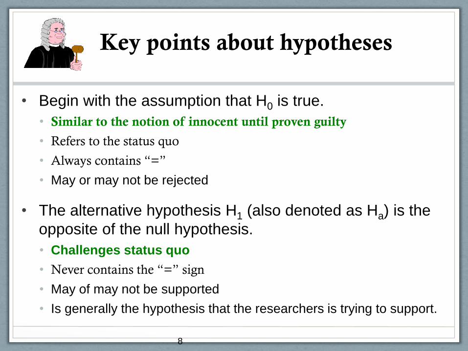
Key points about hypotheses
• Begin with the assumption that H0 is true.
• Similar to the notion of innocent until proven guilty
• Refers to the status quo
• Always contains “=”
• May or may not be rejected
• The alternative hypothesis H1 (also denoted as Ha) is the
opposite of the null hypothesis.
• Challenges status quo
• Never contains the “=” sign
• May of may not be supported
• Is generally the hypothesis that the researchers is trying to support.
8

9
Classical hypothesis testing steps
• Step 1 – Formulate hypotheses H0 and H1. E.g. H0: μ= 29 vs. H1: μ≠ 29
• Step 2 – Choose the significance level for the test, α =0.05
• Step 3 – Decide on statistical test, gather data and do any checks required
by the test.
• Step 4 – Calculate the test statistic
• Step 5a – Decision via p-values. Refer the value of the test statistic to a
known distribution which it would follow if H0 were true.. Then calculate
the probability p (p-value) of obtaining a test statistic such as ours or one
even more extreme if H0 were true. If p is small (i.e. smaller than α ) H0 is
rejected in favour of H1. If p large then there is no evidence to suggest H0
should be rejected.
• Step5b–Decision via rejection regions. Find rejection regions i.e. the region
of unlikely values. If test statistics falls in rejection region then reject H0.
• Step 6- State conclusions and interpret the results

T-test (one-sample t-test)
The known distribution which test statistic follows if H0 were true. In t-test this distribution is t-distribution with n-1 degrees of freedom.
10
H0: μ = μ0
H1: μ ≠ μ0
n
x 0
st
2/2/
0
t>t or t- < t if
HReject
0
/2 /2
It is a hypothesis tests for the population mean μ, if population standard
deviation is unknown, if population is Normal and if random sample
was done (i.e. measurement independent of each other).
So the data should be Normally distributed but test statistic has t-distribution…
t

Student’s t-distribution
• t-distribution has one parameter: the
degrees of freedom.
• The picture shows 4 t-distributions.
• The last distribution (df=infinity) is
identical with Normal distribution. They
are virtually same if df=30.
Note: If we have n data values and if we use
it to estimate the population standard
deviation parameter then our data are less
informative as data were we would knew the
population parameter. Specifically, if we
estimate 1 mean, then knowing n-1 data
values we do not need to be told the last data
value as we can calculate it from the n-1 data
values and from their sample mean--- this is
called as having n-1 degrees of freedom.
t-distribution with smaller
degrees of freedom has heavier
tails then normal distribution,
so it allows for higher chance of
values from tails due not
knowing the population
standard deviation.

Example. t-test, Steps 1-4
Solution
• The test is to determine: H0:μ=29, Ha:μ≠29
• We can use the one sample t-test
• It assumes that the distribution is to Normal
• It assumes that we do not know population standard deviation sigma, but
we estimate it by sample standard deviation s
• We will use level of significance α =0.05
• Test statistic is t:
1194.1
20
3135.5
2967.26
n
s
xt

To find rejection region, we need to use Student’s t table (in any stats
book). As the alternative is two tailed alpha must be split: α/2= 0.025.
Because n=20 the degrees of freedom are n-1=20-1=19.
So t19,0.025 =2.093 “critical value”
0
/2 /2
t
-1.1194
-2.093 2.093
Rejection region Rejection region
Example. Step 5b. Decision via rejection region.
Decision:
Do we reject H0?
No, bc value is -1.1194 which is within the
non-rejection region.
Do we accept H0?
No, we only reject or not reject H0. If we
accepted H0 it would mean that true mean is 29,
but we have no idea what it is.

Alternatively we may look for probability of obtaining a test statistic such as
ours or one even more extreme. Such probability is called p-value. If p is
small H0 is rejected in favour of H1 (i.e. smaller then chosen level of
significance). If p large then no evidence to suggest H0 should be rejected
Example. Step 5b. Decision via p-value
How we use p-value to decide if we reject H0?
Pvalue = 0.26> α =0.05 so we will not reject the null hypothesis at the 5%
significance level.
P-value =
2 x (area of tail up to
-2.093)
= 2x 0.13=0.26
t
0
-1.1194
-2.093 2.093 1.1194

Be careful when performing
hypothesis testing

What to be careful about
• Know how to interpret the p-value
• Always heck the assumptions of the test. If they are
not satisfied the results are NOT valid.
• The one sample t-test has assumptions.
• normality of data
• random sample
• data are metric (continuous)
• It is sensitive to outliers

17
Interpretation of P-value
• Interpretation: Probability of observing data such as ours
or data even more extreme if the null hypothesis is true
• Significance level (: cut-off for p) is usually taken to be
5% (1% or 0.1%)
• P < 0.05 => reject the null hypothesis at the 5%
significance level

18
P-value conventions
• P<0.001 => reject H0 at the 0.1% significance level
=> very strong evidence against H0
• P<0.01 => reject H0 at the 1% significance level
=> strong evidence against H0
• P<0.05 => reject H0 at the 5% significance level
=> sufficient evidence against H0
• P>0.05 => cannot reject H0 at the 5% significance level
=> insufficient evidence against H0

19
Misinterpretation of p-values
• a common misinterpretation is that the p-value is the probability that the data have arisen by chance
• We cannot say this since we do not know what the truth is in the population
• We can say that the p-value is the probability of observing the data such as ours or even more extreme if the null hypothesis is true
This comment is general for any statistical hypothesis test.

t-test assumes normal
distribution of the population
• Data that are said to follow the ‘Normal Distribution’ will produce a characteristic single peaked, bell-shaped histogram symmetric about the mean.
• How do we check normal distribution of our population?
• Checking normality visually.
• Histogram
• Boxplot
• Normal probability plots
• Test of normality
• Kolmogorov-Smirnov goodness-of-fit test
• Other tests
),( 2N

Normal distribution with mean
and standard deviation
21
Possible values for the variable x
from the population
(16%) (16%)
(68%) 2
),( 2N

Example. Normality of mfERG
Is the mfERG distribution Normal? Do they appear to be outliers?
It appears that it is symmetric, it does not appear to copy the normal
curve, but that can be due to fact that we have only 20 observations. We
can use a Normality test.
No outliers – by looking at the boxplot.
Boxplot Histogram

Example. Testing the normality of mfERG via KS test
One test to use is Kolmogorov-Smirnov test (KS) of how how well our data match
normal distribtuion. It is a nonparametric test, it calculates deviations between
distribution of our data and of normal distribution.
In SPSS – Analyze – Nonparametric Tests – One Sample, then chose follow
description on the menu. Here we chose “Automatically compare observed data to
hypothesized”.
What are hypotheses of this test?
Ho: Normal distribution H1: Not normal
Is there evidence that distribution of the mfERG is not Normal?
No evidence, bc p=0.98>0.05, hence can not reject H0

The inventor of normal distribution (1809)
Carl Friedrich Gauss (1777-1855), German mathematician and physical scientist. Discovered the normal distribution in as a way to rationalize the method of least squares. The normal distribution is also called “Gaussian distribution”.

25
Two-sided and one-sided hypothesis tests
• Extreme results can occur by chance in either
direction, which is allowed for in a two-sided
test and two-sided p-value
• sometimes it might be thought that the
difference can only occur in one direction,
leading to a one-sided test
• rarely appropriate
• must be specified before data are analysed

26
Two types of error associated
with hypothesis tests
We need to impose reasonable limits on two types of error:
Type I error: =probability of rejecting H0 when in fact H0 is true
Type II error: b =probability of not rejecting H0 when in fact H0 is false
Can not
reject H0
Reject H0
H0 is true correct
decision
Type I error
H0 is false Type II
error b
correct
decision
Note: Power = 1 – b = probability of rejecting H0 when H0 is false. Typically is set to 5% (1% or 0.1%) and b to 10% or 20%, but will vary according to context.

27
Multiple testing
• Each hypothesis test is usually performed allowing there to be a 1 in 20 chance of saying there is a difference between groups when actually there is not (setting to 0.05)
• The chance of finding such a spurious result increases as the number of tests performed increases
• decide on number of comparisons in advance of analysis and adjust p-values using Bonferroni or similar method.
Number of comparisons Probability of at least one
false-positive result
1 0.05
2 0.10
5 0.23
10 0.40
20 0.64
How hypothesis testing links with
other statistical inference tools?

How hypothesis test
links with confidence interval
• Hyp test and conf interval are two key tools of statistical inference
• A confidence interval for the population mean is a range of values which we are confident (to some degree) includes the true value of the population mean
• In Session 2 we constructed 95% confidence interval for mean mfERG: (25.3, 30.0)
• Based on this confidence interval how we decide about H0: mean=29 vs not?
• Since 29 belongs to the confidence interval we decide not to reject H0
29
There is a correspondence between confidence intervals and hypothesis tests.
Why we learn both?
Confidence interval gives answer in original units. Test gives p-values i.e. a
sense how close we are to rejecting null hypothesis..

Example: back to mfERG
Sampling Distribution of X if H0 is true
μ0 = 29 27.67 X
Where on the vertical axis are the unlikely values?
• Outside of 95% conf interval (25.3, 30.0)
How unlikely is the value 27.67?
• P-value=0.26 is giving us the idea here. Obtaining sample mean value
27.67 or more extreme value has probability 0.26 (if population mean
is 29 – which is what we do not know), hence the mean value 27.67 is
not unlikely.

Summary
Hypothesis testing
• is used to make inference about population parameter, and not the sample statistic
• Null hypothesis is always tested, i.e. we try to find if there is an evidence in sample against the null hypothesis
• If we do not find evidence against null hypothesis, then we say that we do not reject the null hypothesis. In such situation these are wrong statements: “null hypothesis is true”, “we accept the null hypothesis”. .
Always check assumptions of tests. If assumptions not satisfied the results of the test are not valid.
Conclusion of test can be found in two ways
• Using critical values that define the rejection region
• Using p-value that defines the probability of observing even more extreme sample if H0 is true
In statistical tests we do two errors: type I and type II
• If prob of type I decreases, then prob of type II error increases…
• We always set Prob of type I error before analyzing sample data.
• One way to have both errors on specific level is by having large enough sample.

Resources
Books
• Practical statistics for medical research by Douglas G. Altman
• Medical Statistics from Scratch by David Bowers
Journals’ with series on how to do statistics in clinical research
• American Journal of Ophthalmology has Series on Statistics
• British Medical Journal has series Statistics Notes
Manual for SPSS statistical software - with lots of worked-out examples
• Andy Field, Discovering statistics using SPSS
Workshops organized by Biostatistics Department, U of Liverpool
• http://www.liv.ac.uk/medstats/courses.htm,
• Design and analysis of laboratory-based studies, 22 April 2013
• Statistical issues in the design and analysis of research projects 15-19 April 2013

Thank you for your attention
These slides and worksheet can be found on: http://pcwww.liv.ac.uk/~czanner/
Planned future workshops:
• How to analyze data if they are not Normal? Nonparametric methods
• How to predict if a patient is having a disease? Classification methods. (june/july)
• How to make sense of many measured characteristics? Multivariate stats methods
• Ideas are welcome!
Statistical Clinics for ophthalmic clinicians and researchers !
Run by appointment.
Email: [email protected]
Phone: +44-151-706-4019
Further information: http://pcwww.liv.ac.uk/~czanner/