PubH 7405: REGRESSION ANALYSIS

INTRODUCTION TO

LOGISTIC REGRESSION

Let Y be the Dependent Variable Y taking on values 0 and 1, and: π = Pr(Y=1) Y is said to have the “Bernouilli distribution” (Binomial with n = 1). We have:

)1()()(

πππ

−==

YVarYE

Consider, for example, an analysis of whether or not business firms have a daycare facility, according to the number of female employees, the size of the firm, the type of business, and the annual revenue. The dependent variable Y in this study was defined to have two possible outcomes: (i) Firm has a daycare facility (Y=1), and (ii) Firm does not have a daycare facility (Y=0).

As another example, consider a study of Drug Use among middle school kids, as a function of gender and age of kid, family structure (e.g. who is the head of household), and family income. In this study, the dependent variable Y was defined to have two possible outcomes: (i) Kid uses drug (Y=1), and (ii) Kid does not use drug (Y=0).

In another example, say, a man has a physical examination; he’s concerned: Does he have prostate cancer? The “truth” would be confirmed by a biopsy. But it’s a very painful process (at least, could we say if he needs a biopsy?) In this study, the dependent variable Y was defined to have two possible outcomes: (i) Man has prostate cancer (Y=1), and (ii) Man does not have prostate cancer (Y=0). Possible predictors include PSA level, age, race.

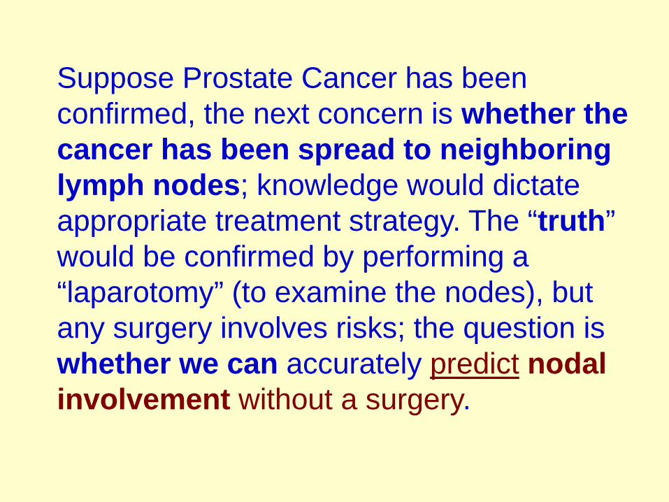
Suppose Prostate Cancer has been confirmed, the next concern is whether the cancer has been spread to neighboring lymph nodes; knowledge would dictate appropriate treatment strategy. The “truth” would be confirmed by performing a “laparotomy” (to examine the nodes), but any surgery involves risks; the question is whether we can accurately predict nodal involvement without a surgery.

In this study, the dependent variable Y was defined to have two possible outcomes: (i) With nodal involvement (Y=1), and (ii) Without nodal involvement (Y=0).

Possible “predictors” include X-ray reading, biopsy result pathology reading (grade), size and location of the tumor (stage - by palpation with the fingers via the rectum), and “acid phosphatase level” (in blood serum).

The basic question is: Can we do “regression” when the dependent variable, or “response”, is binary?

For “binary” Dependent Variables, we run into problems with the “Normal Error Model” – The distribution of Y is Bernouilli. However, the “normal” assumption is not very important (i.e. “robust”); effects of any violation is quite minimal – especially if n is large!

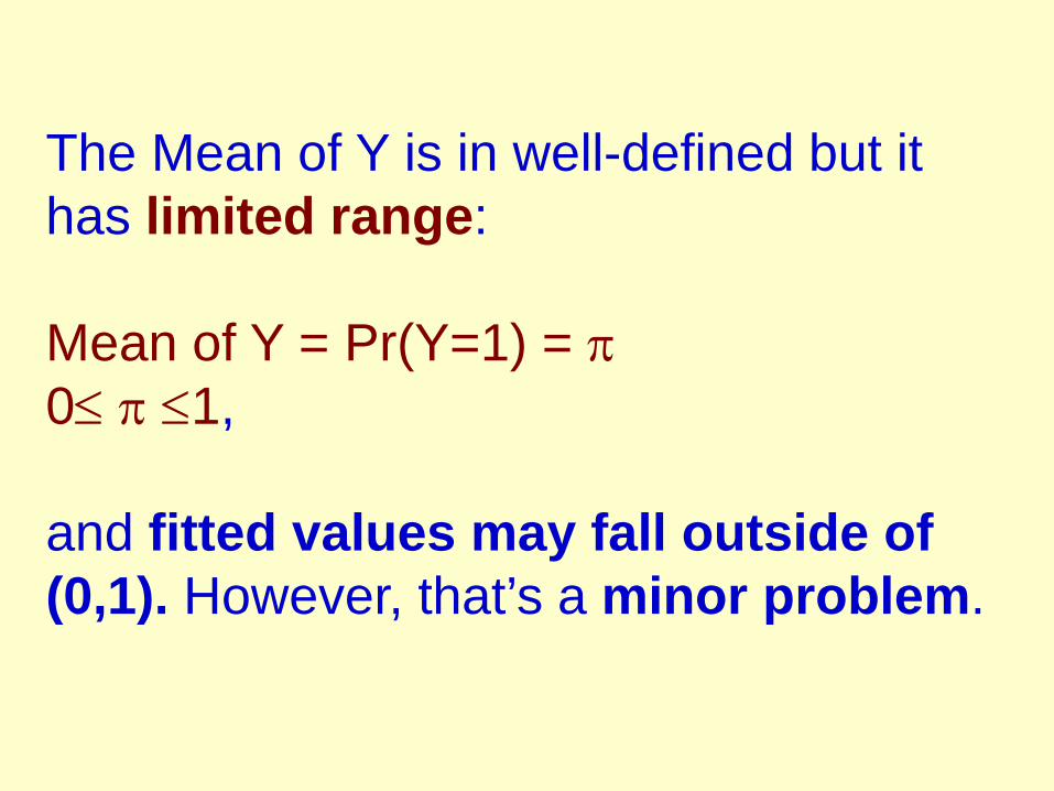
The Mean of Y is in well-defined but it has limited range: Mean of Y = Pr(Y=1) = π 0≤ π ≤1, and fitted values may fall outside of (0,1). However, that’s a minor problem.

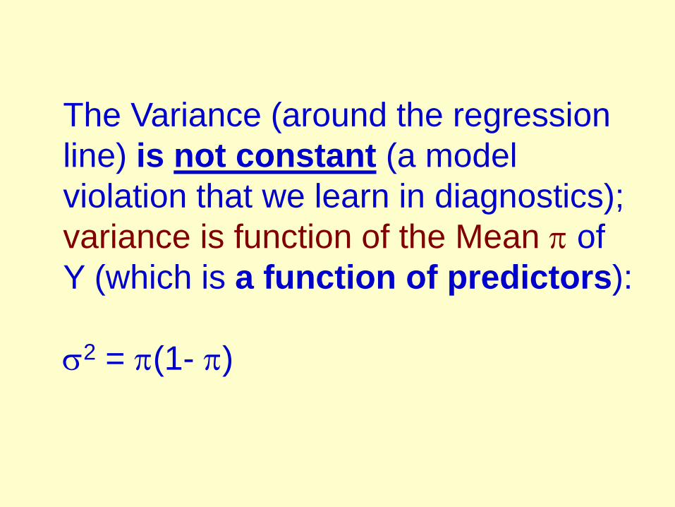
The Variance (around the regression line) is not constant (a model violation that we learn in diagnostics); variance is function of the Mean π of Y (which is a function of predictors): σ2 = π(1- π)

More important, the relationship is not linear. For example, with one predictor X, we usually have:

X

Y

0

1

XXX XX X X X

X X X X XXXXXXX

We still can focus on “modeling the mean”, in this case it is a Probability, π = Pr(Y=1), but the usual linear regression with the “normal error regression model” is definitely not applicable – all assumptions are violated, some may carry severe consequences.

Conclusion: We need some transformation for Y (assumptions about Y are violated)

EXAMPLE: Dose-Response Data in the table show the effect of different concentrations of (nicotine sulphate in a 1% saponin solution) on fruit flies; here X = log(100xDose), just making the numbers easier to read.

Dose(gm/100cc) # of insects, n # killed, r x p (%)0.1 47 8 1.000 17.0

0.15 53 14 1.176 26.40.2 55 24 1.301 43.60.3 52 32 1.477 61.50.5 46 38 1.699 82.60.7 54 50 1.845 92.6

0.95 52 50 1.978 96.2

Proportion p is an estimate of Probability π

EXAMPLE: Dose-Response Data in the table show the effect of different concentrations of (nicotine sulphate in a 1% saponin solution) on fruit flies; here X = log(100xDose), just making the numbers easier to read.

Dose(gm/100cc) # of insects, n # killed, r x p (%)0.1 47 8 1.000 17.0

0.15 53 14 1.176 26.40.2 55 24 1.301 43.60.3 52 32 1.477 61.50.5 46 38 1.699 82.60.7 54 50 1.845 92.6

0.95 52 50 1.978 96.2

p is an increasing function of x; in what way?

UNDERLYING ASSUMPTION It is assumed that each subject/fly has its own tolerance to the drug. The amount of the chemical needed to kill an individual fruit fly, called “individual lethal dose” (ILD), cannot be measured - because only one fixed dose is given to a group of n flies (indirect assay) (1) If that dose is below some particular fly’s ILD, the insect survived. (2) Flies which died are those with ILDs below the given fixed dose.

INTERPRETATION OF DATA • 17% (8 out of 47) of the first

group respond to dose of .1gm/100cc (x=1.0); that means 17% of subjects have their ILDs less than .1

• 26.4% (14 out of 53) of the 2nd group respond to dose of .15gm/100cc (X=1.176); that is 26.4% of subjects have their ILDs less than .15

Dose # n # killed X p(%)0.1 47 8 1.000 17.0

0.15 53 14 1.176 26.40.2 55 24 1.301 43.60.3 52 32 1.477 61.50.5 46 38 1.699 82.60.7 54 50 1.845 92.6

0.95 52 50 1.978 96.2

Interpretation of data:

we view each dose D (with X = log of D) as upper endpoint of an interval and p the cumulative relative frequency

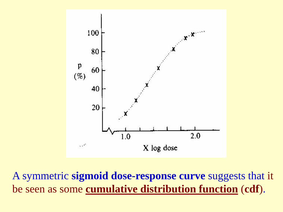
A symmetric sigmoid dose-response curve suggests that it be seen as some cumulative distribution function (cdf).

“Empirical evidence”, i.e. data, suggest that we view p the cumulative relative frequency. This leads to a “transformation” from “π” to an “upper endpoint”, say Z (which is on the continuous scale) corresponding to that cumulative frequency of some cdf. After this transformation, the regression model is then imposed on Z, the transformed value of π.

Let π be the probability “to be modeled” and X a covariate (let consider only one X for simplicity). The first step in the regression modeling process is to obtain “the transformed value Z of π” using the following transformation:

. some is )f( function density yprobabilit

f(u)duor f(u)duπZ

Z

u∫∫

∞

∞−=

MODELING A PROBABILITY

Cumulative Proportion π

1- π

Transformation: π to Z which is on a linear scale

Z

As a result, the proportion π has been transformed into a new variable Z on the “linear” or continuous scale with unbounded range. We can use Z as the dependent variable in a regression model. (We now should only worry about “normality” which is not very important)

The relationship between covariate X (in the example, log of the dose) or covariates X’s and Probability π (through Z) is then stipulated by the usual simple linear regression:

∑=

+=

+=

k

1iii0

10

xββZ

:regression multipleor xββZ

∫∫∞

∞−=

Z

Zf(z)dzor f(z)dzπ

function density yprobabilitneed we: through Z to translateorder toin f(.)

"" a is Allπ

In theory, any probability density function can be used. We can choose one either by its simplicity and/or its extensive scientific supports. And we can check to see if the data fit the model (however, it’s practically hard because we need lots of data to tell).

A VERY SIMPLE CHOICE

0z ;ef(z) z ≥= −

:densitywith on"Distributi lExponentiaUnit " isy possibilitA

Result (for one covariate X) is:

xββln 10 +=

= ∫∞

−−

−

)(10

π

πββ

dzex

z

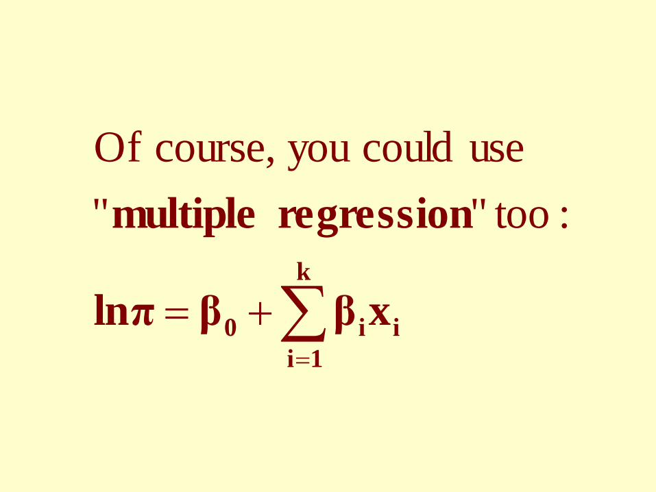
That is to model the “log” of the probability as a “linear function” of covariates.

∑=

+=k

1iii0 xββlnπ

regression multiple : too"" use couldyou course, Of

The advantage of the approach of modeling the “log” of the probability as a “linear function” of covariates, is easy interpretation of model parameters, the probability is changed by a multiple constant (i.e.“multiplicative model” which is usually plausible)

)ln(

ln

lnln

ln:(exposed) 1

ln:)(unexposed 0ln

exp

exp

expexp1

2210exp1

220exp1

22110

Odds

xxxx

xx

osedun

osed

osedunosed

osed

osedun

=

=

−=

++==

+==++=

ππ

ππβ

βββπ

ββπβββπ

binary is XSay :Example 1

REGRESSION COEFFICIENTS

• If X1 is binary (=0/1) representing an exposure, β1 represents the (log of) the “odds” (of having the event represented by Y) associated with the exposure – adjusted for that of X2

• If X1 is on a continuous scale, β1 represents the (log of) the “odds” (of having the event represented by Y) associated with one unit increase in the value of X1 - adjusted for X2

The model is plausible; calculations could be simple too; after the log transformation of “p”, proceeding with usual steps in regression analysis. this approach has a small problem: the exponential distribution is defined only on the whole positive range and certain choice of “x” could make the fitted probabilities exceeding 1.0

x10ln ββπ +=

LOGISTIC TRANSFORMATION

2)]exp(1[)exp()(

:density with (Standard)

θθθ

+=f

onDistributi Logistic

Result is:

)exp(11

)exp(1)exp(

]1[

10

10

10

2

0

x

xx

de

exZ

ββ

ββββ

θπββ

θ

θ

−−+=

+++

=

+= ∫

+=

∞−

xββπ1

πlog

e1eπ

10

xββ

xββ

10

10

+=−

=−

+=−

+=

+

+

+

+

x

x

e

e10

10

1

111

ββ

ββ

ππ

π

We refer to this as “Logistic Regression”

Exponential transformation leads to a linear model of “Log of Probability”: ln(π); Logistic transformation leads to a linear model of “Log of Odds”: ln[π/(1- π)]

When π is small (rare disease/event), the probability and the odds are approximately equal.

OddsOdds

Odds

+=

−=

1

1

π

ππ

Advantages:

(1) Also very simple data transformation: Z = log{p/(1-p)}

(2) The logistic density, with thicker tails as compared to normal curve, may be a better representation of real-life processes.

A POPULAR MODEL • Although one can use the Standard Normal

density in the regression modeling process (or any density function for that purpose),

• The Logistic Regression, as a result of choosing Logistic Density remains the most popular choice for a number of reasons: closed form formula for π, easy computing (Proc LOGISTIC)

• The most important reasons: interpretation of model parameter and empirical supports!

REGRESSION COEFFICIENTS

xP

Px

x

10

10

1ln

)exp(1)exp(

ββ

βαββπ

+=−

+++

=

β1 represents the log of the odds ratio associated with X, if X is binary, or with “an unit increase” in X if X is on continuous scale; β0 only depends on “event prevalence”- just like any intercept.

)(Ratio Odds

lnln

ln:(exposed) 1

ln:)(unexposed 01

ln

binary is XSay :

1

exp

exp

1expexp

2210exp1

220exp1

22110

1

β

β

βββ

ββ

βββπ

π

eOddsOdds

OddsOddsxOddsxxOddsx

xx

osedun

osed

osedunosed

osed

osedun

==

=−

++==

+==

++=−

Example

β1 is the odds ratio on the log scale if X is binary

REGRESSION COEFFICIENTS

• If X1 is binary (=0/1) representing an exposure, β1 represents the (log of) the “odds ratio” (of having the event represented by Y) associated with the exposure – adjusted for that of X2

• If X1 is on a continuous scale, β1 represents the (log of) the “odds ratio” (of having the event represented by Y) associated with one unit increase in the value of X1 - adjusted for X2

Logistic Regression applies in both prospective and retrospective (case-control) designs. In prospective design, we can calculate/estimate the probability of an event (for specific values of covariates). In retrospective design, we cannot calculate/estimate the probability of events because the “intercept” is meaningless but relationship between event and covariates are valid.

SUPPORTS FOR LOGISTIC MODEL The fit and the origin of the linear logistic model could be easily traced as follows. When a dose D of an agent is applied to a pharmacological system, the fractions fa and fu of the system affected and unaffected satisfy the so-called “median effect principle” (Chou, 1976): where ED50 is the “median effective dose” and “m” is a Hill-type coefficient; m = 1 for first-degree or Michaelis-Menten system. The median effect principle has been investigated much very thoroughly in pharmacology. If we set “ π= fa”, the median effect principle and the logistic regression model are completely identical with a slope β1= m.

m

u

a

EDd

ff

=50

Besides the Model, the other aspect where Logistic Regression, both simple and multiple, is very different from our usual approach is the way we estimate the parameters or regression coefficients. The obstacle is the lack of homoscedasticity: we cannot assume a constant variance after the logistic transformation.

P1PlogZ−

=

)1(1

)1()]1([

1

)()]1([

1

)(][)(

2

2

2

pnp

npp

pp

pVarpp

pVardpdZZVar

−=

−−

=

−=

=

Not constant

SOLUTION #1: WEIGHTED LS

Instead of minimizing the “sum of squares”, we minimize the “weighted sum of squares”

Σw[z - (α + βx)]2

where the weight for the value Z is 1/Var(Z). This can be done but much more complicated.

P1PlogZ−

=

In addition, Z might not be defined if p=0 or p=1

SOLUTION #2: MLE

1/0;]exp[1

]}{exp[

)1(

)Pr(L

:Function Likelihood)exp(1

)exp(:Model

1 10

10

1

1

1

10

=++

+=

−=

==

+++

=

∏

∏

∏

=

−

=

=

i

n

i i

yi

yn

ii

yi

i

n

ii

yx

x

yY

xx

i

ii

ββββ

ππ

βαββπ

Maximum Likelihood Estimation (MLE) process gives us estimates of all regression coefficients and their standard errors, bi (estimate of βi) and SE(bi)

TEST FOR SINGLE FACTOR • The question is: “Does the addition of one

particular factor of interest add significantly to the prediction of Pr(Y=1) over and above that achieved by other factors?”.

• The Null Hypothesis for this test may stated as: "Factor Xi does not have any value added to the prediction of the probability of response over and above that achieved by other factors ". In other words,

0:0 =iH β

TEST FOR SINGLE FACTOR

• The Null Hypothesis is • Regardless of the number of variables in the model,

one simple approach is using

• Refer it to the percentiles of the standard normal distribution, where bi is the corresponding estimated regression coefficient and SE(bi) is the standard error of βi , both of which are provided by any computer package.

0:0 =iH β

)SE(bbz

i

i=

ESTIMATING ODDS RATIO

• General form of 95% CI for βi: bi ± 1.96*SE(bi); bi is point estimate of βi, provided by SAS, and SE(bi) from Information matrix, also by SAS

• Transforming the 95% confidence interval for the parameter estimates to 95% C.I. for Odds Ratios:

[ ])(96.1exp ii bSEb ±

Logistic Model For Interaction

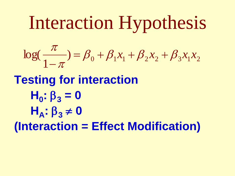
“Usual approach”: use the product of individual terms to represent “interaction” – also called “effect modification”

21322110)1

log( xxxx ββββπ

π+++=

−

Interaction Hypothesis

Testing for interaction H0: β3 = 0 HA: β3 ≠ 0 (Interaction = Effect Modification)

21322110)1

log( xxxx ββββπ

π+++=

−

In summary, with “Logistic Regression”, we “lost” these tools that we use with NERM:

The global F-test

R2 and all coefficients of partial determination (there are some substitutes but not as good)

All graphs (Scatter diagram, all residual plots, and Variable-added Plot)

Least Squares method (but MLE is better)

All other methods/tools are unchanged (test for single factors, stepwise, etc…)

Indirect Assays: Dose fixed, Response random.

Depending on the “measurement scale” for the response (our random variable), we divide indirect assays into two groups:

(1) Quantal assays, where the response is binary: whether or not an event (like the death of the subject) occurs,

(2) Quantitative assays, where measurements for the response are on a continuous scale.

Quantal response assays belong to the class of qualitative indirect assays. They are characterized by experiments in which each level of a stimulus (eg. dose of a drug) is applied to n experimental units; r of them respond and (n-r) do not response.That is “binary” response (yes/no). The group size “n” may vary from dose to dose; in theory, some n could be 1 (so that r = 0 or 1).

From Webster International Dictionary:

“Biological Assay is the estimation of the strength of a drug by comparing its effect on biological material, as animals or animal tissue, with those of a standard product.”

In other words, we (usually) can only estimate “relative potency” of an agent, not its “potency”.

Quantal assays are exceptions to this definition.

QUANTAL ASSAYS VERSUS QUANTITATIVE ASSAYS

• Quantal bioassays are qualitative; we observe occurrences of an event - not obtain measurements on continuous scale.

• Because the event is well-defined, we can estimate agent’s potency. The most popular parameter is the level of the stimulus which result in a response by 50% of individuals in a population. It is often denoted by LD50 for median lethal dose, or ED50 for median effective dose, or EC50 for median effective concentration.

• However, measures of potency depend on the biological system used; the estimates of LD50’s for preparations of the same system can be used to form the relative potency – which would be more likely independent from the system.

The most popular parameter LD50 (for median lethal dose), or ED50 (for median effective dose), or EC50 (for median effective concentration) is the level of the stimulus which result in a response by 50% of individuals in a population. (1) It is a measure of the agent’s potency, which could be used to form relative potency. (2) It is chosen by a statistical reason; for any fixed number of subjects, one would attain greater precision as compared to estimating, say, LD90 or LD10 or any other percentiles.

THE ASSAY PROCEDURE • The usual design consists of a series of dose levels

with subjects completely randomized among/to the dose levels. The experiment may include a standard and a test preparations; or maybe just the test.

• The dose levels chosen should range from “very low” (few or no subjects would respond) to “rather high” (most or all subjects would respond).

• The objective is often to estimate the LD50; the number of observations per preparation depends on the desired level of precision of its estimate – sample size estimation is a very difficult topic.

LOG POTENCY In the logistic the density, if we set p = .5 (or Y=0) we can obtain “log potency” (log of LD50); its estimate is given by, where b0 and b1 are estimated intercept and slope, respectively:

1

^

1

0

0

)50log(

bb

LDM

=

−=

=

ββ[ ]

[ ]

1

0

10

10

10

05.exp1

exp

ββ

ββββ

ββπ

−==

=+⇔=++

+=

Mx

xx

x

med

EXAMPLE AN IN VITRO EXPERIMENT

Cells from a tumor-derived cell line are deposited in wells of a cell culture dish in complete growth medium. After phase growth is established (say, 72 hrs in a typical cell line), wells are treated with different concentrations of a test agent – including a control (i.e. vehicle) well. Doses are spread over a wide range from very low to very high.

The endpoint is “cell survival” and the aim is to establish “potency parameters”.

Unlike Clinical or In Vivo trials; for In Vitro trials, the number of cells at the beginning of the experiment in each well, prior to drug exposure, may be large but unknown; that is why a control (i.e. vehicle) well is needed. (same volume were deposited in wells)

Cells: ALL

Drug: Vincristine

(Extra feature: original and recurrent tumors from the same patient which is not needed here)

Two straight lines: similar intercepts;

Recurrent tumor: smaller slope

Readings & Exercises

• Readings: A thorough reading of the text’s sections 14.1-14.5 (pp.555-581) is highly recommended.

• Exercises: The following exercises are good for practice, all from chapter 14 of text: 14.4, 14.5, and 14.12.

Due As Homework #20.1 Refer to dataset “Prostate Cancer”, let Y = Node and

five independent variables, X1 = X-Ray, X2 = Grade, X3 = Stage, X4 = Age, and X5 = Acid.

a) Fit the model with Acid as the only covariate and interpret the results, including the meaning of the slope.

b) Add more terms to the model in question (a) to test if Stage modifies the effect of Acid

c) In model (a) is the effect of Acid linear? d) Fit the model containing all five covariates and

interpret the results b) In model (d) does Age modifies the effect of Acid?