Introduction to MATLAB 7

for Engineers

William J. Palm III

Chapter 9 Numerical Calculus and Differential Equations

The area A under the curve of f (x) from x = a to x = b.

b A = ∫ f(x) dx

a

Find the following

integral:

A =

∫

sin(x ) dx Fresnel’s cosine integral

2

Illustration of (a) Rectangular and (b) Trapezoidal

numerical integration.

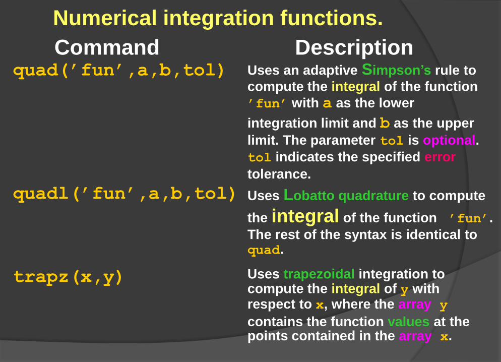
Numerical integration functions.

Command quad(’fun’,a,b,tol)

quadl(’fun’,a,b,tol)

trapz(x,y)

Description Uses an adaptive Simpson’s rule to

compute the integral of the function

’fun’ with a as the lower

integration limit and b as the upper

limit. The parameter tol is optional.

tol indicates the specified error

tolerance. Uses Lobatto quadrature to compute

the integral of the function ’fun’.

The rest of the syntax is identical to quad. Uses trapezoidal integration to compute the integral of y with respect to x, where the array y

contains the function values at the points contained in the array x.

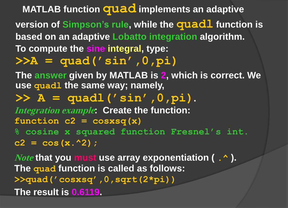
MATLAB function quad implements an adaptive

version of Simpson’s rule, while the quadl function is

based on an adaptive Lobatto integration algorithm.

To compute the sine integral, type:

>>A = quad(’sin’,0,pi)

The answer given by MATLAB is 2, which is correct. We use quadl the same way; namely, >> A = quadl(’sin’,0,pi).

Integration example: Create the function: function c2 = cosxsq(x)

% cosine x squared function Fresnel’s int. c2 = cos(x.^2);

Note that you must use array exponentiation ( .^ ). The quad function is called as follows: >>quad(’cosxsq’,0,sqrt(2*pi))

The result is 0.6119.

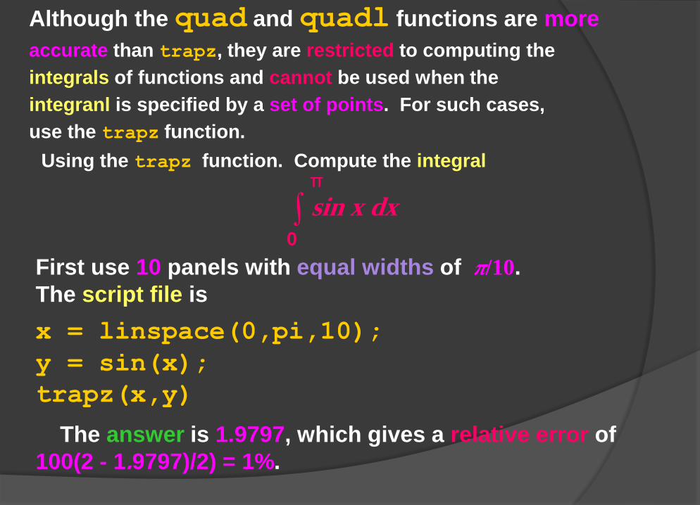
Although the quad and quadl functions are more accurate than trapz, they are restricted to computing the

integrals of functions and cannot be used when the

integranl is specified by a set of points. For such cases,

use the trapz function.

Using the trapz function. Compute the integral π ∫

0

sin x dx

First use 10 panels with equal widths of π/10.

The script file is

x = linspace(0,pi,10);

y = sin(x);

trapz(x,y)

The answer is 1.9797, which gives a relative error of 100(2 - 1.9797)/2) = 1%.

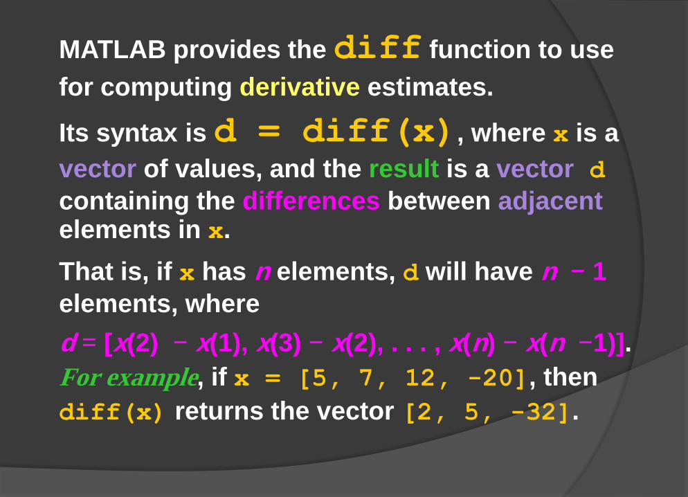
MATLAB provides the diff function to use

for computing derivative estimates.

Its syntax is d = diff(x), where x is a

vector of values, and the result is a vector d

containing the differences between adjacent elements in x. That is, if x has n elements, d will have n − 1

elements, where

d = [x(2) − x(1), x(3) − x(2), . . . , x(n) − x(n −1)].

For example, if x = [5, 7, 12, -20], then

diff(x) returns the vector [2, 5, -32].

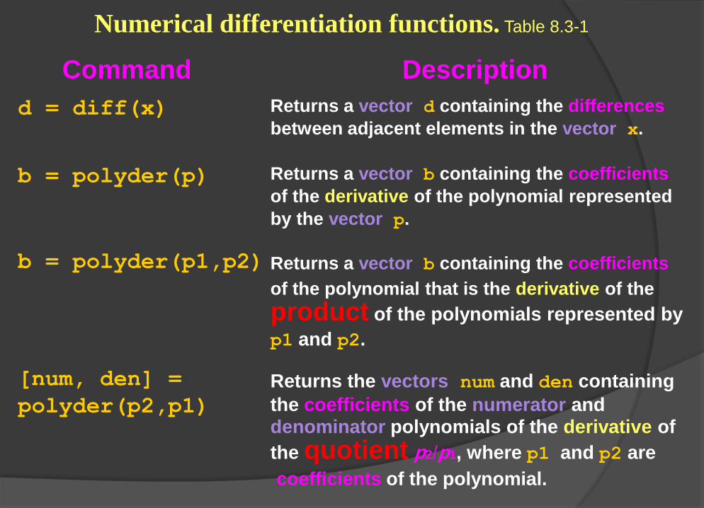
Numerical differentiation functions. Table 8.3-1

Command d = diff(x)

b = polyder(p)

b = polyder(p1,p2)

[num, den] =

polyder(p2,p1)

Description Returns a vector d containing the differences

between adjacent elements in the vector x.

Returns a vector b containing the coefficients

of the derivative of the polynomial represented

by the vector p.

Returns a vector b containing the coefficients

of the polynomial that is the derivative of the

product of the polynomials represented by

p1 and p2.

Returns the vectors num and den containing

the coefficients of the numerator and

denominator polynomials of the derivative of

the quotient p2/p1, where p1 and p2 are

coefficients of the polynomial.

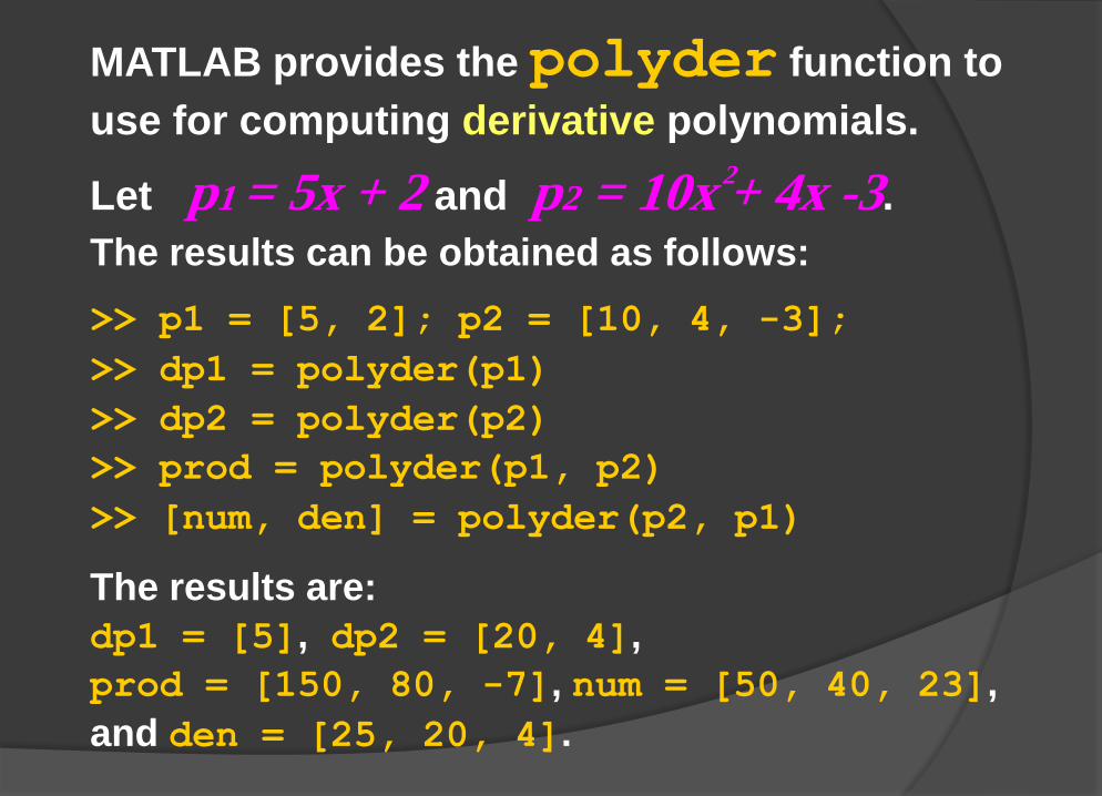
MATLAB provides the polyder function to

use for computing derivative polynomials.

Let p1 = 5x + 2 and p2 = 10x + 4x -3.

The results can be obtained as follows: >> p1 = [5, 2]; p2 = [10, 4, -3];

>> dp1 = polyder(p1)

>> dp2 = polyder(p2)

>> prod = polyder(p1, p2)

>> [num, den] = polyder(p2, p1)

The results are:

dp1 = [5], dp2 = [20, 4], prod = [150, 80, -7], num = [50, 40, 23],

and den = [25, 20, 4].

2

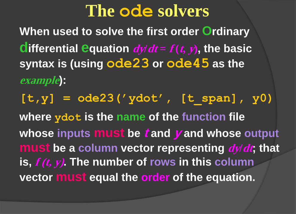
The ode solvers When used to solve the first order Ordinary

differential equation dy/dt = f (t, y), the basic

syntax is (using ode23 or ode45 as the

example): [t,y] = ode23(’ydot’, [t_span], y0)

where ydot is the name of the function file

whose inputs must be t and y and whose output

must be a column vector representing dy/dt; that

is, f (t, y). The number of rows in this column

vector must equal the order of the equation.

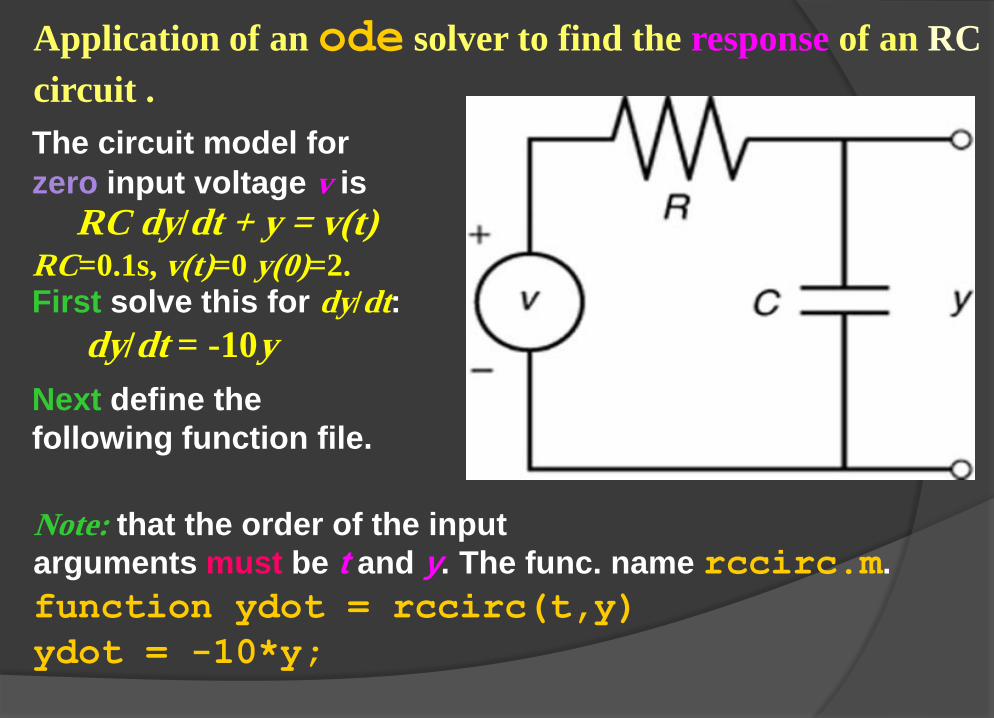
Application of an ode solver to find the response of an RC

circuit . The circuit model for

zero input voltage v is

RC dy/dt + y = v(t) RC=0.1s, v(t)=0 y(0)=2.

First solve this for dy/dt:

dy/dt = -10y Next define the following function file.

Note: that the order of the input arguments must be t and y. The func. name rccirc.m.

function ydot = rccirc(t,y)

ydot = -10*y;

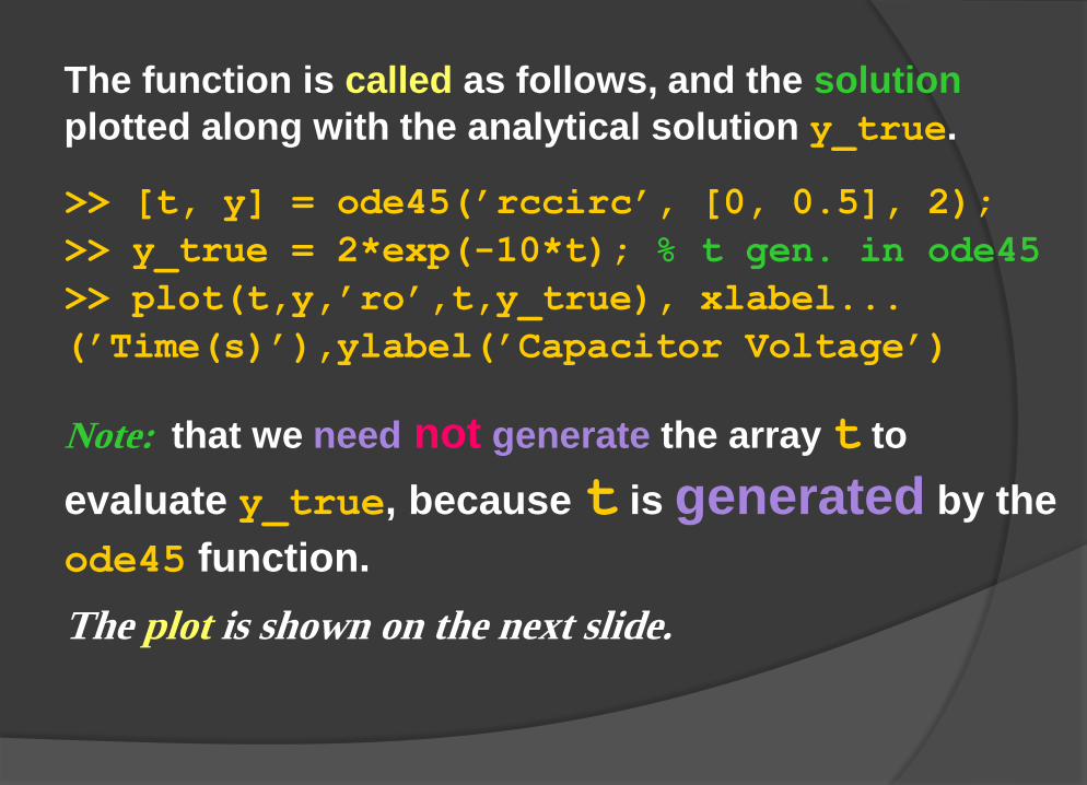
The function is called as follows, and the solution

plotted along with the analytical solution y_true.

>> [t, y] = ode45(’rccirc’, [0, 0.5], 2);

>> y_true = 2*exp(-10*t); % t gen. in ode45

>> plot(t,y,’ro’,t,y_true), xlabel...

(’Time(s)’),ylabel(’Capacitor Voltage’)

Note: that we need not generate the array t to

evaluate y_true, because t is generated by the

ode45 function. The plot is shown on the next slide.

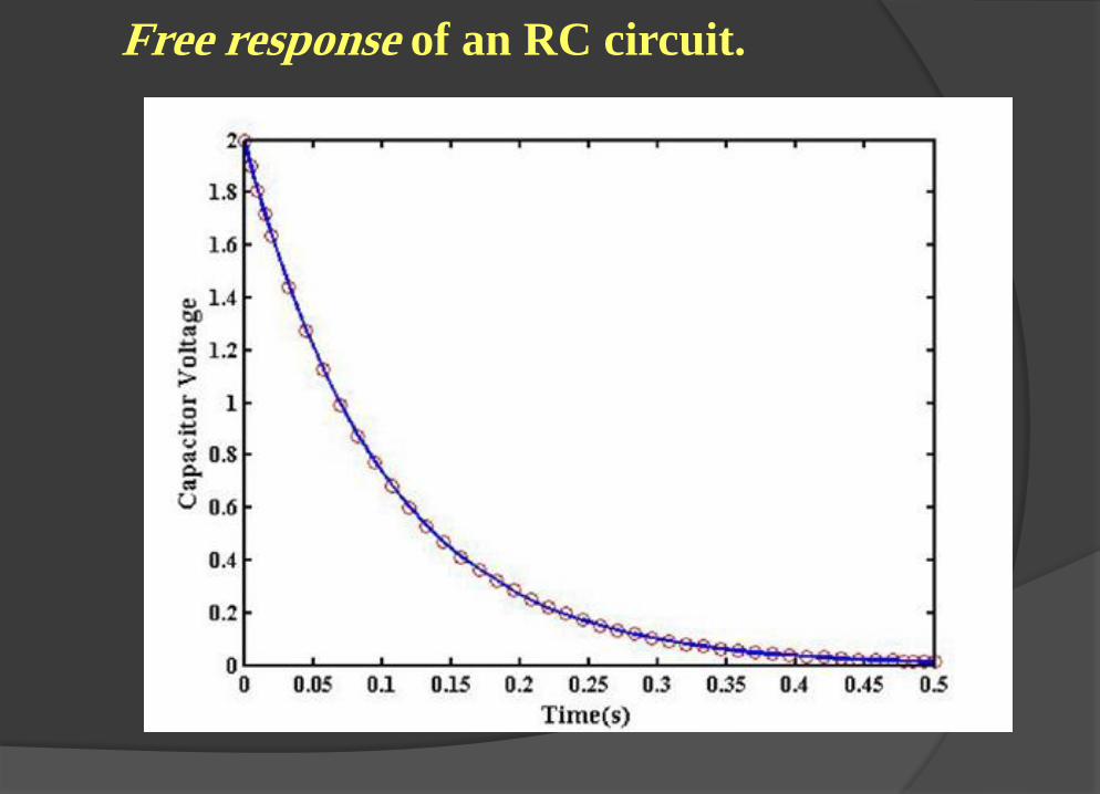
Free response of an RC circuit.

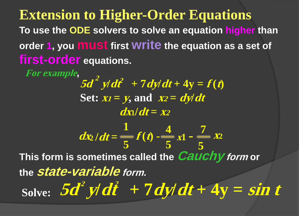
Extension to Higher-Order Equations To use the ODE solvers to solve an equation higher than

order 1, you must first write the equation as a set of

first-order equations.

For example, 5d y/dt + 7dy/dt + 4y = f (t)

Set: x1 = y, and x2 = dy/dt

dx1/dt = x2

1 dx f (t) -

4 7

x2

2 /dt = 5 5

5 This form is sometimes called the Cauchy form or

the state-variable form.

Solve:

5d y/dt + 7dy/dt + 4y = sin t

2 2

x1 -

2 2

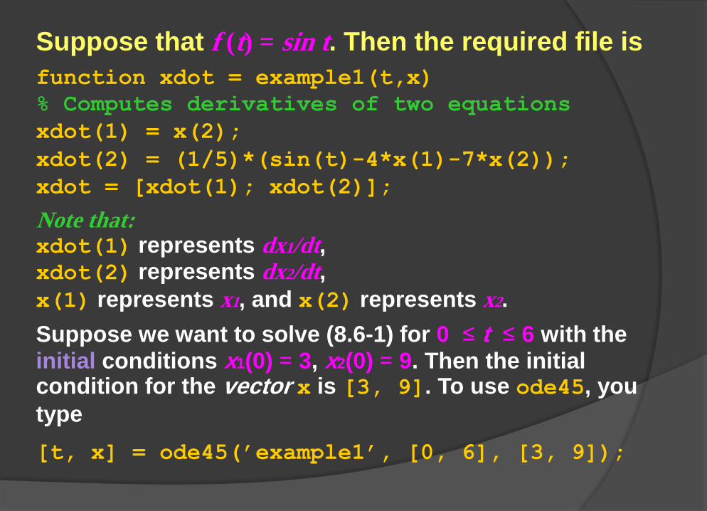
Suppose that f (t) = sin t. Then the required file is function xdot = example1(t,x) % Computes derivatives of two equations

xdot(1) = x(2);

xdot(2) = (1/5)*(sin(t)-4*x(1)-7*x(2));

xdot = [xdot(1); xdot(2)];

Note that: xdot(1) represents dx1/dt, xdot(2) represents dx2/dt,

x(1) represents x1, and x(2) represents x2. Suppose we want to solve (8.6-1) for 0 ≤ t ≤ 6 with the initial conditions x1(0) = 3, x2(0) = 9. Then the initial condition for the vector x is [3, 9]. To use ode45, you

type [t, x] = ode45(’example1’, [0, 6], [3, 9]);

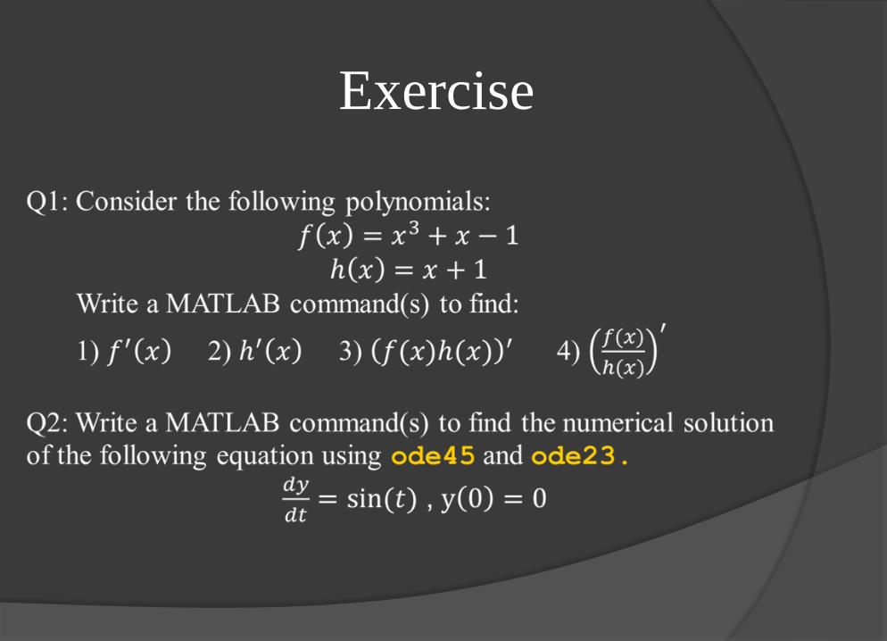
Exercise