Embed Size (px)
Citation preview

8/11/2019 Introduction to Mechatronics - Appuu Kuttan.pdf
http://slidepdf.com/reader/full/introduction-to-mechatronics-appuu-kuttanpdf 1/345
Introduction to
MECHATRONICS
APPUU KUTTAN K.K.Professor
Department of Mechanical EngineeringNational Institute of Technology Karnataka
Surathkal

8/11/2019 Introduction to Mechatronics - Appuu Kuttan.pdf
http://slidepdf.com/reader/full/introduction-to-mechatronics-appuu-kuttanpdf 2/345
OXFORDUNIVERSITY PRESS
Oxford University Press is a department of the University of Oxford.It furthers the University's objective of excellence in research, scholarship,
and education by publishing worldwide in
Oxford New YorkAuckland Cape Town Dar es Salaam Hong Kong KarachiKuala Lumpur Madrid Melbourne Mexico City Nairobi
New Delhi Shanghai Taipei Toronto
With offices inArgentina Austria Brazil Chile Czech Republic France Greece
Guatemala Hungary Italy Japan Poland Portugal SingaporeSouth Korea Switzerland Thailand Turkey Ukraine Vietnam
Oxford is a registered trade mark of Oxford University Pressin the UK and in certain other countries.
Published in Indiaby Oxford University Press
© Oxford University Press 2007
The moral rights of the authors have been asserted
Database right Oxford University Press (maker)
First published 2007Third impression 2010
All rights reserved. No part of this publication may be reproduced,
stored in a retrieval system, or transmitted, in any form or by any means,without the prior permission in writing of Oxford University Press,
or as expressly permitted by law, or under terms agreed with the appropriatereprographics rights organization. Enquiries concerning reproduction
outside the scope of the above should be sent to the Rights Department,Oxford University Press, at the address above.
You must not circulate this book in any other binding or coverand you must impose this same condition on any acquirer.
ISBN-13: 978-0-19-568781-1ISBN-10: 0-19-568781-7
Typeset in Times Romanby Text-o-Graphics, Noida 201301
Printed jn India by Ram Book Binding House, New Delhi 110020and published by Oxford University Press
YMCA Library Building, Jai Singh Road, New Delhi 110001
8/11/2019 Introduction to Mechatronics - Appuu Kuttan.pdf
http://slidepdf.com/reader/full/introduction-to-mechatronics-appuu-kuttanpdf 3/345
Mechatronics refers to the multidisciplinary approach comprising mechanics, electronics, and computer
technology that aims at improving the performance and quality of engineering products. Mechatronics
today has found numerous applications in designing, manufacturing, and maintenance of a wide
range of engineering products. A lot of devices we see around, such as DVD players, washing
machines, and microwave ovens, are products of mechatronic engineering.
In the past, only one form of technology was used in designing and manufacturing of mechanical
devices. But now a synergistic integration of mechanical, electronics and computer engineering
disciplines is being used to produce efficient devices. The application of mechatronic concepts enhances
the productivity and quality of the products. Apart from automobiles, consumer electronics,
telecommunications and robotics, mechatronic systems are today also being used in biomedicine andaerospace industries. Mechatronics is fast developing as the core of all the activities in production
technology.
The subject of mechatronics is also becoming increasingly popular in engineering colleges for research
as well as education. Research topics related to mechatronics are diverse and include actuators/
sensors, microelectromechanical systems (MEMS), mechatronic devices/machines, etc. Engineering
colleges are also updating their courses in mechatronics to equip the students with the essential tools
to successfully face today’s industrial challenges. Mechatronics, thus, has a key role to play in future
technological advancements.
About the Book
Introduction to Mechatronics provides a complete coverage of the basic principles of mechatronics
and their applications. Beginning with the basic concepts, the book moves on to cover the topics such
as system modelling and analysis, microprocessors, microcontrollers, sensors, actuators, need of
intelligent systems for accurate operation of mechatronic systems, and applications of mechatronic
systems in autotronics, bionics, and avionics. Case studies on slip casting for ceramic products and
pick-and-place robots enhance the value of the text.
Preface

8/11/2019 Introduction to Mechatronics - Appuu Kuttan.pdf
http://slidepdf.com/reader/full/introduction-to-mechatronics-appuu-kuttanpdf 4/345
Content and Coverage
The book comprises eleven chapters and two appendices. Exercises are provided at the end of each
chapter to help the readers assess their comprehension of the subject matter studied in the chapter.
Ample number of examples are interspersed throughout the text to illustrate the concepts.
Chapter 1 contains an introduction to mechatronics and its applications and objectives. The advantages
and disadvantages of mechatronics are also discussed.
Chapter 2 begins with a discussion on the challenges faced by today’s manufacturing industries and
then deals with computer integrated manufacturing and just-in-time production systems.
Chapter 3 discusses force, friction, and lubrication in detail as also stress–strain behaviour, bending
of beams and torsion. The chapter also includes fits and tolerance, surface texture and scraping, and
machine structure.
Chapter 4 introduces the readers to the applications of electronics in mechatronics. Conductors,insulators, and semiconductors along with digital, passive, and active electrical components are
discussed comprehensively in this chapter.
Chapter 5 covers various analog and digital computers as well as analog to digital and digital to
analog conversions. Microprocessor, microcontroller, and programmable logic controller (PLC) are
also described in this chapter.
Chapter 6 commences with a description of the control system concept. It further discusses time
response of a system, frequency domain analysis, and the modern control theory. Sequential and
digital control systems are also included in this chapter.
Chapter 7 deals with the motion control devices, i.e. the elements of mechatronic systems responsible
for transforming the output of a microprocessor or a control system into a controlling action on a
machine or device. Hydraulic, pneumatic and electrical actuators as well as DC servomotor, AC
servomotor, and stepper motor are described at length in this chapter along with brushless permanent
magnet DC motors and microactuators.
Chapter 8 focusses on various types of internal and external sensors. The working principles of
some microsensors are also presented in this chapter.
Chapter 9 deals with computer numerical control (CNC) and direct numerical control (DNC) machines.It discusses at length the CNC machine operation.
Chapter 10 provides a detailed description of the applications of intelligent systems in designing of
mechatronic systems. Designing principles of some consumer mechatronic products—such as washing
machine, automatic camera, and alarm indicator—are dealt with to make the subject matter practice-
oriented. This chapter also includes case studies on the slip casting process and pick-and-place
robots.
iv Preface

8/11/2019 Introduction to Mechatronics - Appuu Kuttan.pdf
http://slidepdf.com/reader/full/introduction-to-mechatronics-appuu-kuttanpdf 5/345
Chapter 11 discusses three major specialized study areas of mechatronics, namely, autotronics
bionics, and avionics.
There are two appendices at the end of the book. Appendix A lists Laplace transforms of different
time domain functions. Appendix B has a table comparing Laplace and Z transforms.
The book is designed as a textbook for undergraduate students of mechanical, electronics, and
electrical engineering disciplines. In addition, it will also prove to be useful for postgraduate students
as well as practising engineers.
Acknowledgements
I sincerely thank the editorial team of Oxford University Press for the help provided to me in bringing
out this book. I am also grateful to the reviewers who reviewed my manuscript and offered comments
that greatly enhanced the quality of the book.
APPUU KUTTAN K.K
Preface v

8/11/2019 Introduction to Mechatronics - Appuu Kuttan.pdf
http://slidepdf.com/reader/full/introduction-to-mechatronics-appuu-kuttanpdf 6/345
Contents
Preface iii
Chapter 1 Mechatronic Systems 1
1.1 Synergy of Systems 1
1.2 Definition of Mechatronics 3
1.3 Applications of Mechatronics 5
1.4 Objectives, Advantages, and Disadvantages of mechatronics 9
Illustrative Examples 10
Exercises 11
Chapter 2 Mechatronics in Manufacturing 12
2.1 Production Unit 12
2.2 Input/Output and Challenges in Mechatronic Production Units 13
2.3 Knowledge Required for Mechatronics in Manufacturing 16
2.4 Main Features of Mechatronics in Manufacturing 17
2.5 Computer Integrated Manufacturing 21
2.6 Just-in-Time Production Systems 22
2.7 Mechatronics and Allied Subjects 23
Illustrative Examples 23
Exercises 26
Chapter 3 Mechanical Engineering and Machines in Mechatronics 27
3.1 Force, Friction, and Lubrication 27
3.2 Behaviour of Materials Under Load 32
3.3 Materials 38
3.4 Heat Treatment 38
8/11/2019 Introduction to Mechatronics - Appuu Kuttan.pdf
http://slidepdf.com/reader/full/introduction-to-mechatronics-appuu-kuttanpdf 7/345
viii Contents
3.5 Electroplating 39
3.6 Fits and Tolerance 39
3.7 Surface Texture and Scraping 40
3.8 Machine Structure 41
3.9 Guideways 42
3.10 Assembly Techniques 44
3.11 Mechanisms used in Mechatronics 44
Illustrative Examples 52
Exercises 56
Chapter 4 Electronics in Mechatronics 57
4.1 Conductors, Insulators, and Semiconductors 57
4.2 Passive Electrical Components 584.3 Active Elements 65
4.4 Digital Electronic Components 72
Illustrative Examples 78
Exercises 81
Chapter 5 Computing Elements in Mechatronics 82
5.1 Analog Computer 83
5.2 Timer 555 85
5.3 Analog to Digital Conversion 86
5.4 Digital to Analog Conversion 88
5.5 Digital Computer 89
5.6 Architecture of a Microprocessor 91
5.7 Microcontroller 94
5.8 Programmable Logic Controller 95
5.9 Computer Peripherals 97
Illustrative Examples 105
Exercises 109
Chapter 6 Systems Modelling and Analysis 110
6.1 Control System Concept 112
6.2 Standard Test Signals 118
6.3 Time Response of A System 120
6.4 Block Diagram Manipulation 130
6.5 Automatic Controllers 132
8/11/2019 Introduction to Mechatronics - Appuu Kuttan.pdf
http://slidepdf.com/reader/full/introduction-to-mechatronics-appuu-kuttanpdf 8/345
Contents ix
6.6 Frequency Domain Analysis 134
6.7 Modern Control Theory 135
6.8 Sequential Control System 141
6.9 Digital Control System 141
Illustrative Examples 147
Exercises 149
Chapter 7 Motion Control Devices 151
7.1 Hydraulic and Pneumatic Actuators 152
7.2 Electrical Actuators 160
7.3 DC Servomotor 166
7.4 Brushless Permanent Magnet DC Motor 169
7.5 AC Servomotor 1707.6 Stepper Motor 171
7.7 Microctuators 172
7.8 Drive Selection and Applications 176
Illustrative Examples 179
Exercises 183
Chapter 8 Sensors and Transducers 185
8.1 Static Performance Characteristics 186
8.2 Dynamic Performance Characteristics 187
8.3 Internal Sensors 189
8.4 External Sensors 195
8.5 Microsensors 207
Illustrative Examples 213
Exercises 215
Chapter 9 CNC Machines 216
9.1 Adaptive Control Machine System 2209.2 CNC Machine Operations 221
Exercises 246
Chapter 10 Intelligent Systems and Their Applications 248
10.1 Artificial Neural Network 249
10.2 Genetic Algorithm 257
10.3 Fuzzy Logic Control 260
10.4 Nonverbal Teaching 263

8/11/2019 Introduction to Mechatronics - Appuu Kuttan.pdf
http://slidepdf.com/reader/full/introduction-to-mechatronics-appuu-kuttanpdf 9/345
x Contents
10.5 Design of Mechatronic Systems 264
10.6 Integrated Systems 268
Case Study 10.1: Slip Casting Process 277
Case Study 10.2: Pick-and-Place Robot 282
Exercises 285
Chapter 11 Autotronics, Bionics, and Avionics 286
11.1 Autotronics 286
11.2 Bionics 300
11.3 Avionics 309
Exercises 316
Appendix A: Laplace Transform 317
Appendix B: Laplace and Z Transforms 319
Bibliography 320
Index 327

8/11/2019 Introduction to Mechatronics - Appuu Kuttan.pdf
http://slidepdf.com/reader/full/introduction-to-mechatronics-appuu-kuttanpdf 10/345
Mechatronic Systems
1.1 Synergy of Systems
The quest for making life better, easier, and comfortable has been at the heart of
all the endeavours by human beings. All inventions and innovations have one
aim, that of making life comfortable. In this pursuit, human beings have gone
beyond exploiting only the basic sciences for producing technology products
that are in tune with their aim. The technological advancement that we see
today is a product of putting together some or all the basic sciences. This has
resulted in as diverse and useful products as human beings can go in exploiting
the knowledge base. This technological advancement has made it possible toproduce products that can substitute for human effort. There are two forms of
human effort: physical effort and mental effort. Technology is, accordingly,
classified as machine technology and fine technology. Machine technology aims
at relieving physical stress and strain of human beings. Some examples of the
products of this category are machine tools, power generators, pumps, etc. Fine
technology, on the other hand, is concerned with relieving mental strain of human
beings. Measuring systems, computers, communication systems, etc., come
under this category.
Communication and information transfer is vital to put together machinetechnology and fine technology. A combination of these can offer both physical
and mental prowess. A combination of these two technologies has produced
products that can substitute for human element in both its facets, physical effort
and mental effort.
Typewriter has the distinction of being the first communication system ever
used. Typewriter is purely a mechanical system. The first patent of a typewriter
was made by Henry Mill in the year 1714. Until 1830 patents were made for
typewriters working with different constructions. In 1864 Peter Mitter Hofer, a

8/11/2019 Introduction to Mechatronics - Appuu Kuttan.pdf
http://slidepdf.com/reader/full/introduction-to-mechatronics-appuu-kuttanpdf 11/345
2 Introduction to Mechatronics
carpenter, made the first typewriter which resembled the modern type writer. In
1874 onwards, industrial production of typewriter started. Even today, most of
the data transfer systems use the typewriter keyboard as the basic input device.
French philosopher Rene Descarts (1596–1650) found the relation between
algebra and geometry. He illustrated the theory in a graph an algebraic function.It was the basis for analytical geometry. Later another French mathematician
Cocagne prepared a monogram. Solutions to different mathematical calculations
could be obtained with the help of the monogram.
But the accuracy of such calculations depended upon the accuracy of the drawing
of monogram and the behaviour of the paper with respect to atmospheric
humidity and temperature. In the course of time, mechanical linkages were
developed to make calculations with greater accuracy, ease, and speed. Computer
is the most advanced and accurate system for making large and repetitive
calculations today. The focus now is on developing an interface capable of
feeding data at a rate that is compatible with the computer’s ability to process
data.
The human can communicate directly or indirectly with the computer. Direct
communication means that information is entered into the computer by means
of switches on a console, or by using the enquiry typewriter. The information is
received from the computer in the form of visual displays or audible alarms or
printed matter. Indirect communication involves an intermediate medium such
as magnetic type, punched card, or magnetic disk or compact disk. Indirectcommunication is necessary because of the great mismatch in speed between
human input and computer consumption.
Traditional mechanical systems were built using mechanical components only.
In the steam engine, James Watt used steam energy to convert it into kinetic
energy by the rotational motion of shaft using a reciprocating mechanism. The
speed of steam flow was controlled by a fly-ball governor. This is an example
of a mechanical feedback system. In the twentieth century, electrical energy
and electric signals were made available for industrial applications. These proved
more efficient in the conversion of electrical energy into mechanical energy
because electrical energy is easier to process as signals for measurement and
control. Consider a mechanical system such as a shaper machine which removes
material during the forward stroke only. In this system, the backward stroke is
made faster since metal removal does not take place during a backward stroke.
The time required for the backward stroke can be minimized using computer
and electronic gadgets. This provides minimum cycle time and better production
rate. The last few decades have seen digital computers taking place of most of

8/11/2019 Introduction to Mechatronics - Appuu Kuttan.pdf
http://slidepdf.com/reader/full/introduction-to-mechatronics-appuu-kuttanpdf 12/345
Mechatronic Systems 3
the analog devices. Faster and more accurate results are obtained using a digital
computer. As a result, most of the production processes and products are a mix
of mechanical, electrical, and digital components. The design and manufacture
of mixed systems requires the knowledge from all these disciplines. Mechatronics
is the science that deals with mechanical, electrical, and digital componentsneeded for the mixed systems. An inter-disciplinary knowledge is must for
specialized engineers in mechanical, electrical, or digital systems.
1.2 Definition of Mechatronics
The integration of mechanical engineering, electronics engineering and computer
technology is increasingly forming a crucial part in the design, manufacture
and maintenance of a wide range of engineering products and processes. As a
consequence of the synergy of systems in industry, it is becoming increasinglyimportant for engineers and technicians to adopt an interdisciplinary and
integrated approach towards engineering problems. The term ‘mechatronics’ is
used to describe this integrated approach. In the design of cars, robots, machine
tools, washing machines, cameras, microwave ovens, and many other machines,
an integrated and interdisciplinary approach to engineering design is increasingly
being adopted.
The term ‘mechatronics’ was first coined by the Japanese scientist Yoshikaza
in 1969. The trademark was accepted in 1972. Mechatronics is a subject whichincludes mechanics, electronics, and informatics (Fig. 1.1).
Mechanics involves knowledge of mechanical engineering subjects, mechanical
devices, and engineering mechanics. Basic subjects such as lubricants, heat
transfer, vibration, fluid mechanics, and all other subjects studied under
mechanical engineering directly or indirectly find application in mechatronic
systems. Mechanical devices include simple latches, locks, ratchets, gear drives,
and wedge devices to complicated devices such as harmonic and Norton drives,
crank mechanisms, and six bar mechanisms used for car bonnets.
Engineering mechanics discusses the kinematics and dynamics of machine
elements. Kinematics determines the position, velocity, and acceleration of
machine links. Kinematic analysis helps to find the impact and jerk on a machine
element. Change in momentum, causes an impact, whereas change in
acceleration causes a jerk . Dynamic analysis gives the torque and force required
for the motion of link in a mechanism. In dynamic analysis, friction and inertia
play an important role.

8/11/2019 Introduction to Mechatronics - Appuu Kuttan.pdf
http://slidepdf.com/reader/full/introduction-to-mechatronics-appuu-kuttanpdf 13/345
4 Introduction to Mechatronics
Mechanics Electronics
Informatics
Fig. 1.1 Concept of mechatronics
Electronics involves measurement systems, actuators, power electronics, and
microelectronics. Measurement systems, in general, are made of three elements,
namely, the sensor, signal conditioner, and display unit. A sensor responds to
the quantity being measured, giving an electrical output signal that is related to
the input quantity. The signal conditioner takes the signal from the sensor and
manipulates it into conditions which is suitable for either display or control any
other systems. In a display system, the output from the signal conditioner isdisplayed. Actuation systems comprise the elements which are responsible for
transforming the output from the control system into the controlling action of a
machine or device. Power electronic devices are important in the control of
power-operated devices to actuate through a small gate power of the order
milliwatts. The silicon controlled rectifier (thyristor) is an example of a power
electronic device which is used to control dc motor drives. The technology of
manufacturing microelectronic devices through very large scale integrated
(VLSI) circuit designs is also gathering momentum. Microsensors and
microactuators are subdomains of the mechatronic system, which are used inmany applications.
Informatics includes automation, software design, and artificial intelligence.
The programmable logic controller (PLC) or microcontroller, or even personal
computers, are widely used as informatic devices. A completely automated plant
reduces the burden on human beings in respect of decision-making and plant
maintenance, among other things. Software is used not only for solving complex
engineering problems but also in finance systems, communication systems, or
8/11/2019 Introduction to Mechatronics - Appuu Kuttan.pdf
http://slidepdf.com/reader/full/introduction-to-mechatronics-appuu-kuttanpdf 14/345
Mechatronic Systems 5
virtual modelling. Wide area networks, such as internet facilities, have large
data storage facilities and the data can be retrieved from anywhere in the world.
Informatics systems can make decisions using artificial intelligence. Artificial
neural networks, genetic systems, fuzzy logic, hierarchical control systems, and
knowledge-base systems are effective tools used in artificial intelligence.
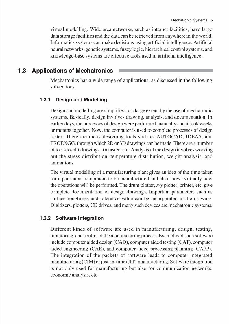
1.3 Applications of Mechatronics
Mechatronics has a wide range of applications, as discussed in the following
subsections.
1.3.1 Design and Modelling
Design and modelling are simplified to a large extent by the use of mechatronic
systems. Basically, design involves drawing, analysis, and documentation. In
earlier days, the processes of design were performed manually and it took weeks
or months together. Now, the computer is used to complete processes of design
faster. There are many designing tools such as AUTOCAD, IDEAS, and
PROENGG, through which 2D or 3D drawings can be made. There are a number
of tools to edit drawings at a faster rate. Analysis of the design involves working
out the stress distribution, temperature distribution, weight analysis, and
animations.
The virtual modelling of a manufacturing plant gives an idea of the time taken
for a particular component to be manufactured and also shows virtually how
the operations will be performed. The drum plotter, x - y plotter, printer, etc. give
complete documentation of design drawings. Important parameters such as
surface roughness and tolerance value can be incorporated in the drawing.
Digitizers, plotters, CD drives, and many such devices are mechatronic systems.
1.3.2 Software Integration
Different kinds of software are used in manufacturing, design, testing,
monitoring, and control of the manufacturing process. Examples of such software
include computer aided design (CAD), computer aided testing (CAT), computer
aided engineering (CAE), and computer aided processing planning (CAPP).
The integration of the packets of software leads to computer integrated
manufacturing (CIM) or just-in-time (JIT) manufacturing. Software integration
is not only used for manufacturing but also for communication networks,
economic analysis, etc.

8/11/2019 Introduction to Mechatronics - Appuu Kuttan.pdf
http://slidepdf.com/reader/full/introduction-to-mechatronics-appuu-kuttanpdf 15/345
6 Introduction to Mechatronics
1.3.3 Actuators and Sensors
Mechanical, electrical, hydraulic, and pneumatic actuators are widely used in
the industry. Toggle linkage and quick return mechanics are typical examples
of mechanical actuators. Switching devices, solenoid-type devices, and drivessuch as alternative current (ac) and direct current (dc) motors can be used as
electrical actuators. Hydraulic and pneumatic drives use linear cylinders and
rotary motors as actuators.
The term sensor is used for an element which produces a signal relating to the
quantity being measured. For example, an electrical resistance temperature
device transforms the input of temperature into change in resistance. The term
transducer is often used in place of sensor. Transducers are defined as devices
which when subject to some physical change experience a related change. Inthe displacement transducer, force is not an error. Addition of extra force into
the system reduces backlash and play. For example, in the dial gauge, an
additional tension spring is provided on the rack so that the play between the set
of gear trains is minimized. Similarly, in a force-transmitting transducer, the
provision of more displacement is not an error. Reduction in the play in force-
transmitting devices produces a loss in power due to friction.
1.3.4 Intelligent Control
Feedback control systems are widespread not only in nature and the home but
also in industry. There are many industrial processes and machines which control
many variables automatically. Temperature, liquid level, fluid flow, pressure,
speed, etc. are maintained constant by process controllers. Adaptive control
and intelligent manufacturing are the areas where mechatronic systems are used
for decision making and controlling the manufacturing environment.
1.3.5 Robotics
Robot technology uses mechanical, electronic, and computer systems. A robot
is a multifunctional reprogrammable machine used to handle materials, tools,
or any special items to perform a particular task. Manipulation robots are capable
of performing operations, assembly, spot welding, spray painting, etc. Service
robots such as mail service robots, household servant robots, nursing robots in
hospitals are being used nowadays.

8/11/2019 Introduction to Mechatronics - Appuu Kuttan.pdf
http://slidepdf.com/reader/full/introduction-to-mechatronics-appuu-kuttanpdf 16/345
Mechatronic Systems 7
1.3.6 Manufacturing
In the domain of factory automation, mechatronics has had far-reaching effects
in manufacturing. Major constituents of factory automation include computer
numerically controlled (CNC) machines, robots, automation systems, and
computer integration of all functions of manufacturing. Low volume, morevariety, higher levels of flexibility, reduced lead time in manufacture, and
automation in manufacturing and assembly are likely to be the future needs of
customers, and mechatronic systems will play an important role in this context.
1.3.7 Motion control
A rigid body can have a very complex motion which might seem difficult to
describe. However, the motion of any rigid body can be considered to be
combinations of translational and rotational motions. By considering a three-dimensional space, a translational movement can be considered to be one which
can be resolved into components along one or more of three axes. The rotation
of a rigid body has rotating components about one or more of the axes. A complex
motion may be a combination of translational and rotational motion. Motion
control is important in many industrial applications such as robots, automated
guided vehicles, NC machines, etc. If the robot arm cannot reach a particular
location, then the movements of workpiece have to be analysed further. Any
body has six degrees of freedom, three translations and three rotations. A point
has only three translations. In a machine tool, the workpiece has six degrees of
freedom and the tools also have six degrees of freedom. Thus, a machine toolwith twelve degrees of freedom can be manufactured. Such a tool can perform
a complicated machining operation.
1.3.8 Vibration and Noise Control
When a machine member is subjected to a periodic dynamic force, it will vibrate.
If the vibration level ranges from a frequency of 20 Hz to 20,000 Hz, it produces
noise. Vibration and noise isolation are important in industry. Vibration isolation
can be achieved by passive, semi-active, or active dampers. In passive dampersthe structure is mounted on damping materials with initial spring loading. In
semi-active dampers, both passive and active damping elements are used. In
active damping, extra energy is used to damp the structure. When a structure is
subjected to a pulse input, a shock is produced. Different types of shock absorbers
are used to reduce the shock amplitude.
Noise isolation is equally important in industry since noise is harmful to human
beings. Adaptive control techniques are used for noise isolation. In this method,
the system predicts the noise level in each interval of time and noise is introduced

8/11/2019 Introduction to Mechatronics - Appuu Kuttan.pdf
http://slidepdf.com/reader/full/introduction-to-mechatronics-appuu-kuttanpdf 17/345
8 Introduction to Mechatronics
through the speaker in phase opposition. This adaptive control system reduces
the noise level.
1.3.9 Microsystems
It is fair to say that microsystems are a major step towards the ultimate
miniaturization of machines and devices such as dust-size computers and needle-
type robots. The advancement of nanotechnology will certainly result in the
realization of superminiaturized machinery. The need for miniaturization has
increased manifold in recent years, and engineering systems and devices have
become more and more complex and sophisticated. Picosatellites, spacecrafts,
table-top manufacturing units, and microelectromechanical systems will become
a reality in the future. The knowledge of mechatronics is very useful for
microsystems.
1.3.10 Optics
All slip gauge blocks are calibrated against light wavelength as a standard.
Angle gauges can be calibrated to an accuracy of 0.1 sec using a light wave
standard—the angstrom unit. A combination of optical and electronic principles
has led to the development of instruments such as the midarm which measures
angular displacement with an accuracy of 0.05 sec. Optical angle measurement
systems for inertial guidance with an accuracy of 0.02 sec have been in use
since 1961. Opto-electronic systems use a lens or telescope to form an opticalimage of an object under study on a photocathode image detector tube. The
motion of the object causes the motion of the photocathode optical image and
the corresponding motion of the electron image. The optical image is obtained
by a conventional videcon camera or a coupled charge device. The camera
converts an array of analog signals, in 236 ¥ 236 pixels in a square centimetre.
The analog signals are then converted into digital signals for each pixel and
transmitted to an electron image grabber to produce an electron image. As the
image starts deviating from the neutral position, the photo multiple layer output
tends to drive back by means of a deflection coil. Thus, any main object can be
brought to the aperture continuously.
The application of still and motion picture photography often allows qualitative
and quantitative analyses of complex motion. The photoelastic method is
convenient to determine the stress distribution in a machine element. The basic
phenomenon of double refraction under load is used in photoelasticity. Double
refraction takes place when light travels at a different speed in a transparent
material depending on the direction of travel relative to the direction of the
principle stress and also depending on the magnitude of the difference between
principle stresses for two-dimensional fields. Due to double refraction, light
8/11/2019 Introduction to Mechatronics - Appuu Kuttan.pdf
http://slidepdf.com/reader/full/introduction-to-mechatronics-appuu-kuttanpdf 18/345
Mechatronic Systems 9
waves form an interference pattern of fringes on a photograph. The photograph
is then used to determine the principal stresses. By the use of the frozen stress
technique, the method can be extended to three-dimensional problems.
The cathode ray tube provides display devices for computers and other
entertainment devices such as the television, projector, etc. Electron guns withbasic columns can be obtained in a pixel. Cathode ray tubes for picture displays
usually have 256 ¥ 256 pixels/cm2. As the number of pixels increases per square
centimetre, the clarity of the picture becomes better. Systems are available
which permit each pixel in grey levels (256 levels) in a black-and-white display.
Grey levels (light intensity levels) are called grey scaling. With the basic three
colours 2563 colour combinations can be obtained with grey scaling.
In the ordinary film, only the magnitude of intensity is recorded, which in turn
gives two-dimensional images. By recording the amplitude and phase of the
reflected light from an object, a hologram can be obtained. A hologram gives
three-dimensional ghost images of three-dimensional objects. An optical
computer with a hologram will give faster computation in future. Coding and
decoding is not required as in conventional computer operation. A ghost image
from the hologram gives a grey-scaled image on each voxel. 2563 voxels can be
accommodated in a cubic centimetre of laser hologram. Sintering in each voxel
can be obtained by packing the metal particles in the ghost image. Thus in
future any complicated article can be manufactured in seconds using the laser
hologram technique.
1.4 Objectives, Advantages, and Disadvantages of Mechatronics
The objectives of mechatronics are the following.
1. To improve products and processes
2. To develop novel mechanisms
3. To design new products
4. To create new technology using novel concepts
Earlier the domestic washing machine used cam-operated switches in order to
control the washing cycle. Such mechanical switches have now been replaced
by microprocessors. A microprocessor is a collection of logic gates and memory
elements whose logical functions are implemented by means of software. The
application of mechatronics has helped to improve many mass-produced products
such as the domestic washing machine, dishwasher, microwave oven, cameras,
watches, and so on. Mechatronic systems are also used in cars for active
suspension, antiskid brakes, engine control, speedometers, etc. Large-scale
8/11/2019 Introduction to Mechatronics - Appuu Kuttan.pdf
http://slidepdf.com/reader/full/introduction-to-mechatronics-appuu-kuttanpdf 19/345
10 Introduction to Mechatronics
improvements have been made using mechatronic systems in flexiblemanufacturing engineering systems (FMS) involving computer controlled
machines, robots, automatic material conveying and, overall supervisory control.
There are many advantages of mechatronic systems. Mechatronic systems have
made it very easy to design processes and products. Application of mechatronicsfacilitates rapid setting up and cost effective operation of manufacturing facilities.
Mechatronic systems help in optimizing performance and quality. These can be
adopted to changing needs.
Mechatronic systems are not without their disadvantages. One disadvantage is
that the field of mechatronics requires a knowledge of different disciplines.
Also, the design cannot be finalized and safety issues are complicated in
mechatronic systems. Such systems also require more parts than others, and
involve a greater risk of component failure.
Illustrative Examples
Example 1.1 An electrical switch is a man-made mechatronic system,
used to control the flow of electricity. The toggle of the switch is a
mechanical system and the human brain or a control system used to actuate
the switch acts as an informatics system. The brain or informatics system
decides whether we need to turn on the switch. If we do, the brain controls
the movement of our limbs and we turn on the switch. When the switch ison, the resistance of contact is nearly zero and energy flow takes place.
When the switch is off, the resistance is infinity and no current flows.
Example 1.2 A thermostatically controlled heater or furnace is a
mechatronic system. The input to the system is the reference temperature.
The output is the actual temperature. When the thermostat detects that the
output is less than the input, the furnace provides heat until the temperature
of the enclosure becomes equal to the reference temperature. Then the
furnace is automatically turned off. Here, the bimetallic strip of the
thermostat acts as informatics since it automatically turns the switch on oroff. The lever-type switch is mechanical system whereas the heater acts as
an electrical system.
Example 1.3 Most washing machines are operated in the following
manner. After the clothes to be washed have been put in the machine, the
soap, detergent, bleach, and water are put in required amounts. The washing
and wringing cycle time is then set on a timer and the washer is energized.
When the cycle is completed, the machine switches itself off.

8/11/2019 Introduction to Mechatronics - Appuu Kuttan.pdf
http://slidepdf.com/reader/full/introduction-to-mechatronics-appuu-kuttanpdf 20/345
Mechatronic Systems 11
When the required amount of detergent, bleach, water, and appropriate
temperature are predetermined and poured automatically by the machine
itself, then the machine is a mechatronic system. The microprocessor used
for this purpose acts as the informatics system. The electrical motor actuated
for wriggling is an electrical system. The agitator and timer are mechanicalsystems. The washing machine is an ideal example of a mechatronic system.
Example 1.4 The automatic bread toaster is a mechatronic system, in
which two heating elements supply the same amount of heat to both sides
of the bread. The quality of the toast can be determined by its surface
colours. When the bread is toasted, the colour detector sees the desired
colours, and the switch automatically opens and a mechanical lever makes
the bread pop up. Mechanical, electrical, and informatics systems are
involved in the operation of the bread toaster.
Exercises
1.1 Identify mechanics, informatics, and electronic systems of the (a) washing
machine, (b) jet engine, (c) bread toaster, and (d) automatic camera.
1.2 What is meant by the kinematic and dynamic analyses of a machine
element?
1.3What are the tools for artificial intelligence?
1.4 Define impact and jerk.
1.5 Identify the areas where mechatronic systems can be used.
1.6 Explain the objectives of mechatronics.
1.7 What are the advantages and disadvantages of a mechatronic system?

8/11/2019 Introduction to Mechatronics - Appuu Kuttan.pdf
http://slidepdf.com/reader/full/introduction-to-mechatronics-appuu-kuttanpdf 21/345
Mechatronics in Manufacturing
2.1 Production Unit
Industrial production is a transformation process that converts raw material into
finished products. The products are made by a combination of manual labour, machinetools, and energy. This transformation process involves a sequence of steps, each
step bringing the material closer to the desired final state. Individual steps form part
of what is called the product operation. Depending on the nature of the product
operation, there are two types of industries.
1. Manufacturing industries—examples are car, computer, machine tool, and
aircraft industries.2. Process industries—examples are petroleum refineries, food-processing,
chemical, and plastic industries.
In the nineteenth century and before, a nation was considered powerful on the basis
of its human resources. The industrial revolution made a change in this. And, in thetwentiethcentury, which was the era of machine power, mechanical advancementdetermined a country’s power. Productivity and growth were the need of the hour.
In the twenty-first century, knowledge is considered to be the indicator of growth.The success of a business is now determined by how efficiently, creatively, and
accurately it uses the knowledge available to it. Application of the knowledge availableis essential for all manufacturing units.
The term ‘knowledge worker’ was first used in 1960. The growth of information
technology and electronics brought about great changes in almost all walks of life.
Knowledge is different from all other kinds of resources. This resource constantly
makes itself obsolete. Knowledge is of two types:
1. Explicit knowledge—which is codable, and in which communication through
data, formulae, etc. is possible, and

8/11/2019 Introduction to Mechatronics - Appuu Kuttan.pdf
http://slidepdf.com/reader/full/introduction-to-mechatronics-appuu-kuttanpdf 22/345
Mechatronics in Manufacturing 13
2. Tacit knowledge—highly personal, hard to formulate, and difficult to
communicate or share with others. Welding and painting are examples of tacit
knowledge.
Knowledge creation is a process of interaction between explicit and tacit knowledge.
For the transformation of tacit knowledge into explicit knowledge, a company shouldcreate an environment to enhance knowledge.
New knowledge is created by an individual, but the organization has to facilitate theadoption of such knowledge. The acquisition of knowledge can create a significant
competitive advantage over other companies in the market. In the domain ofproduction unit automation, mechatronics has had far-reaching effects inmanufacturing and will become even more important in the future.
Major constituents of mechatronic automation involve CNC machines, robots,automation systems, and computer integration of all functions of manufacturing.
Basically, these advanced manufacturing solutions consist of mechatronic systems.
2.2 Input/Output and Challenges in Mechatronic Production Units
Figure 2.1 illustrates the block diagram of a production unit with inputs,challenges, and product output. The inputs are men, machines, material, money,market, and methods. The challenges are competition, communication,commitment, compatibility, and cost. Productivity can be improved byovercoming the challenges, and by technology-based utilization of the six inputs.
Globalization has led to increase in competition. The success of an enterprisedepends on the integration of management technology and human-resourcemanagement. Along with effective use of information technology, this would
enhance productivity of technology and management.
Production unitInput Output
Challenges
Fig. 2.1 Production unit
An intelligent manufacturing system based on machines equipped with artificial
intelligence can handle, compare, and vary conditions without interrupting theautomatic operation. Small and medium-size enterprises require a low-cost
module or computer integrated manufacturing design and system.
8/11/2019 Introduction to Mechatronics - Appuu Kuttan.pdf
http://slidepdf.com/reader/full/introduction-to-mechatronics-appuu-kuttanpdf 23/345
14 Introduction to Mechatronics
Availability of the material plays an important role in production. Usually material
cost per product cannot be reduced unless an alternative material is made. But a
major reduction in cost can be achieved by reduction in transportation time.
An organization’s economic power is dependent upon the level and growth rate of
its productivity. Economists use indexes to measure productivity. The various
measures for productivity are labour productivity index, capital productivity
index, energy productivity index, and material productivity index.
In the last few decades, market and consumer needs have changed significantly.
The priorities in decision making have also changed. In the 1970s a competitive
price was the topmost priority in decision making. But quality took centre stage
in the 1980s and 1990s when cost and quality became essential parameters for
any product to come to the market and delivery and speed assumed a pivotal
role for decision making. The new consumers of this century expect uniquenessand personalized features in products.
Technology should provide a service or product ensuring that the consumer
expends a minimum amount of energy, material, and other resources. At the
same time, the process of production and the product itself should cause
minimum environment pollution. The product and services are the main outputs
from a production unit. However, unwanted scrap and waste are also produced
in this unit. These should also be converted into useful by-products. The
technology involved in such conversion is known as green technology. All greentechnology essentially improves the environment with the following concepts:
1. Reduce,
2. Recycle, and
3. Reuse.
Reducing involves a minimum input of energy and production of minimum
waste material, which is released into the enviroment, while producing the
maximum possible output of the desired product. The recycling of used or
discarded equipment and other items is now being practised to an increasingextent in developed countries. A company can organize itself by properly
codifying and classifying the process waste that it generates, so that it can be
sent to appropriate agencies or end users. Many consumable items which get
contaminated or degraded due to use can be recycled. It is not uncommon to
find a whole lot of equipment of all sizes and complexities and spare being
consigned to the scrapyard in industries because they are either worn out or
beyond repair.

8/11/2019 Introduction to Mechatronics - Appuu Kuttan.pdf
http://slidepdf.com/reader/full/introduction-to-mechatronics-appuu-kuttanpdf 24/345
Mechatronics in Manufacturing 15
Reconditioning is currently in vogue. It involves the use of vintage equipment rather
than new equipment of the same design and productivity.
The new competitive era forced organizations to meet the challenges of staying
technologically competitive in a fully globalized environment. It is evident that
harnessing the technology has become of paramount importance for the successof any enterprise. As the process of globalization has spread, leading to an
increasing need for competitiveness, management of technology has assumedgreater importance. Gradually, the success or even survival of an enterprise willpredominantly depend upon how much technology-driven the organization
becomes. To meet the demands of global competitiveness, an enterprise has todevelop the ability to respond to market demands for changes in productionspecification and product mix as rapidly as possible.
An accountant essentially takes a costing approach to productivity. Engineers
generally seek costing as a measure of the physical asset and other resources,such as production per hour, work hours per unit, material requirement per unit,
machine utilization, and spare utilization. Cost reduction is the most importantpriority for the management. Managers frequently use the accountancy ratiofor achieving the objective of the general management. However, these are notbasic standards according to which production may be measured in differentsituations.
Communication in a manufacturing environment refers to the adequate and
timely flow of information with a feedback mechanism. The purpose of effective
communication is to achieve a better understanding between the employeesand management. Such communication helps to motivate the employees toimprove productivity. The communication technique may not have a short-termimpact on total productivity, but certainly has a positive effect in the long run.Modern methods of communication are paving the way for tele-service and
will lead to increased productivity. The distinct feature of many Japanesecompanies is that they keep even the lowest level employee well informed abouttheir financial status, realizing that all the employees and management are partof one company family whose objective is to produce products or services atthe most competitive price and best quality possible. The employee knows that
if this is not done, there will be no company and no job.
Commitment from employees can be achieved by training and education, andby creating and maintaining an environment in which people can accomplishgoals efficiently and effectively. Training seeks to achieve required humanproductivity by increasing the ability level of the workforce. Some of the commonforms of training are on-the-job training, outside courses, and visitation training.From childhood onwards, all of us have been educated about our surroundings.
The industrial employees—workers, engineers, and managers—should have acertain level of formal or informal education. Different solutions to a given

8/11/2019 Introduction to Mechatronics - Appuu Kuttan.pdf
http://slidepdf.com/reader/full/introduction-to-mechatronics-appuu-kuttanpdf 25/345
16 Introduction to Mechatronics
problem are proposed by different people because of their education levels. Educationis the levels of knowledge one should possesses from visual observations, thinking,and perception of surrounding world. Improving working conditions also helps improve
productivity. This involves a detailed analysis of working conditions. The factorsthat must be analysed are temperature, light, humidity, noise level, colour of the
surroundings, how hazardous material is handled, etc. With the advancement ofrobotics, working conditions can be improved to a great extent.
Environment compatibility, national compatibility, and production compatibility playan important role in any enterprise. National policy and political influence play an
important role in production and production compatibility. The International ProductStandards are important for both hardware and software so that better compatibilitycan be achieved.
The integration of culture plays an important role in improving productivity. Religious,
social, and cultural integration plays an important role in this context. There shouldbe some established process for transforming the skills, ideas, and knowledge among
various cultures.
2.3 Knowledge Required for Mechatronics in Manufacturing
Until the 1970s, machine tools were largely mechanical systems with very limited
electrical or electronic content. However, since then there has been a dramatic
change in technology with an increase in the content of electrical and electronic
systems integrated with mechanical parts through mechatronics. Machine tools
incorporating computer numerical control, electric servodrives, electronic
measuring systems, and precision mechanical parts such as ball screws and
antifriction guideways are examples of the application of mechatronic
technology. The Japanese machine tool industry has flourished because Japanese
have mastered electronics and have been able to combine precision mechanics
and informatics in design. Computer and control system units are widely used
in machine tools. Figure 2.2 shows how the Japanese have incorporated
mechatronics in manufacturing. Computer aided design (CAD), electro-
mechanical devices, control circuitry, and digital control systems are widely
used in mechatronic systems in the manufacturing environment.
The development of computer numerically controlled (CNC) machines is an
outstanding contribution to manufacturing industries. It has made possible the
automation of the machining processes with flexibility to handle small to medium
batch qualities in part production. Initially, the CNC technology was applied on
basic metal cutting machines such as lathes and milling machines. Later, to
increase the flexibility of machines handling a variety of components and to

8/11/2019 Introduction to Mechatronics - Appuu Kuttan.pdf
http://slidepdf.com/reader/full/introduction-to-mechatronics-appuu-kuttanpdf 26/345
Mechatronics in Manufacturing 17
incorporate them in a single set-up in the same machine, CNC machines with material
handling systems were developed. CNC machines are capable of performing multiple
operations such as milling, drilling, boring, and tapping.
Mechanical Electronics
Computer Control
Computer-aided design
Controlcircuitry
Digital control systems
Electromechanical devices
Fig. 2.2 Mechatronics in manufacturing
2.4 Main Features of Mechatronics in Manufacturing
We will discuss the main features of mechatronics in manufacturing in this section.
2.4.1 Flexible Manufacturing System
The flexible manufacturing system was first conceptualized for machines and it
required the prior development of numerical control. The concept is credited toParid Williamson, a British engineer employed by Moliars during the mid 1960s.
Moliars patented the invention. A flexible manufacturing system (FMS) is a
highly automated group-technology machine cell consisting of a group of
processing workstations—usually CNC machine tools, interconnected by an
automated material handling and storage system, and controlled by a distributed
computer system. The reason the FMS is called flexible is that it is capable of
processing a variety of different part styles simultaneously at various
workstations. To qualify as being flexible, a manufacturing system should satisfy
several criteria.
1. Part variety test—the system should be able to process different part stylesin a non-batch mode.
2. Schedule change test—the system should readily adopt to changes inproduct schedule.
3. Error recovery test—the system should be able to recover in the case ofequipment malfunctioning and breakdown.

8/11/2019 Introduction to Mechatronics - Appuu Kuttan.pdf
http://slidepdf.com/reader/full/introduction-to-mechatronics-appuu-kuttanpdf 27/345
18 Introduction to Mechatronics
4. New part test—the system should be able to introduce new part
designs into the existing product.
The types of flexibility in manufacturing are those relating to the machine,
production, mix, product, routing, volume, and expansion. Flexible
manufacturing systems can be distinguished according to the kind of operationsthey perform—process operations or assembly operations. They can also be
distinguished according to the number of machines in the system. A single
machine cell (SMC) consists of one CNC machining centre combined with a
part storage system for unaltered operations. The cell can be designed to operate
in a batch mode, a flexible mode, or in a combination of the two. A flexible
manufacturing cell (FMC) consists of two or three processing workstations—
typically, CNC machining centres or turning centres, which plan a part handling
system to control the loading or unloading station. In addition, the handling
system usually includes a limited part storage capacity. A flexible manufacturing
system has four or more processing workstations connected mechanically by a
common part-handling system and electronically by a distributed computer
system. The benefits that can be expected from the FMS include:
1. increased machine utilization,
2. fewer machine requirements,
3. reduction in factory shopfloor requirement,
4. reduced inventory requirements,
5. greater responsiveness to change,
6. lower manufacturing load time,
7. reduced direct labour requirements and high labour productivity, and
8. opportunity for unattended production.
Load Unload
Load Unload
(a) Inline layout
(b) Loop layout

8/11/2019 Introduction to Mechatronics - Appuu Kuttan.pdf
http://slidepdf.com/reader/full/introduction-to-mechatronics-appuu-kuttanpdf 28/345
Mechatronics in Manufacturing 19
``````````````````````````
Machine station
(c) Robot-centred layout
Fig. 2.3 FMS layouts
The material handling system establishes the FMS system. Most layout configurations
found in today’s FMS’s can be divided into five categories—(a) inline layout, (b)
loop layout, (c) robot-centred layout, (d) ladder layout, (e) open-field layout, which
are shown in Fig. 2.3.

8/11/2019 Introduction to Mechatronics - Appuu Kuttan.pdf
http://slidepdf.com/reader/full/introduction-to-mechatronics-appuu-kuttanpdf 29/345
20 Introduction to Mechatronics
One additional component in the FMS is human labour. Humans are needed to
manage the operations of the FMS. The functions typically performed by humans
include (a) loading new materials, (b) unloading finished parts, (c) changing
and setting the tools, (d) equipment maintenance and repair, (e) NC part
programming, (f) operating the computing system, and (g) overall managementof the system. The status report provides an instantaneous snapshot of the
condition of FMS.
2.4.2 Manufacturing Automatic Protocol
The information and documentation that constitute the product design flow into
the manufacturing and planning function. The information processing activators
in the planning of manufacturing include process planning, master scheduling,
material requirement planning, and capacity planning. Process planningcomprises determining the sequence of individual process and the assembly
operation needed to produce the part. Manufacturing planning includes logistic
issues, commonly known as production planning. The master schedule is the
list of the products to be made. Based on the master schedule, the individual
components and sub-assemblies of each sub-product must be planned. The raw
material must be purchased or requisitioned from the storage department, and
purchase requirements of spare parts must be ordered from suppliers. The entire
task is called material requirement planning. Capacity planning is concernedwith planning the human and machine resources of the firm.
Manufacturing control is concerned with managing and controlling the physical
operation in the factory to carry out manufacturing plans. Manufacturing control
functions include shopfloor control, inventory control, and quality control.
Shopfloor control deals with the problem of monitoring the progress of the
product as it is being processed, assembled, moved, and inspected in the factory.
Inventory control attempts to strike a proper balance between the danger of too
little inventory and the carrying cost of too much inventory. The mission ofquality control is to ensure that the quality of the product and its components
meet the standards specified by the product designer.
The elements discussed above can be automated. Automation can be defined as
a technology concerned with the application of mechanics, electronics,
computers, and control systems to operate and control production. The automated
elements of a production system are said to comprise manufacturing automatic
protocol.
8/11/2019 Introduction to Mechatronics - Appuu Kuttan.pdf
http://slidepdf.com/reader/full/introduction-to-mechatronics-appuu-kuttanpdf 30/345
Mechatronics in Manufacturing 21
2.4.3 Technical Office Protocol
Business functions are the principal means of communicating with the customer.
They form the beginning and end of the information processing cycle. Business
functions include sales and marketing, sales forecasting, order entry, cost
accounting, customer billing, and payroll. It is most important for any businessenterprise to cater to the customer’s needs. This can be done in the following
ways.
1. Through an interview—either by in-person or over telephone.
2. Through comment cards—these allow the customer to give a feedback
regarding the level of sophistication of the product and service.
3. Through a formal survey—this is accomplished by mass mailing.
4. Through focus groups—several customers or potential customers serveon the panel.
5. Through study of complaints—this is a statistical review of data on
customer complaints.
6. By seeking information about the reason why a customer has returned a
product.
7. Through the Internet—this is a relatively new way of gathering customer
opinion.
8. Through field intelligence—this involves the collection of second-handinformation from employees who deal directly with the customer.
Quality function deployment is a systematic procedure for defining customer
needs and interpreting them in terms of product features and process
characteristics. The automation of a business function is called technical office
protocol.
2.5 Computer Integrated Manufacturing
The ideal computer integrated manufacturing (CIM) system applies computer
and communication technology to all of the operational functions and information
processing functions in manufacturing from order receipt, through design and
production, to packaging and shipment. The scope of CIM is compared with the
more limited scope of CAD/CAM in Fig. 2.4. CIM involves an integration of
all the functions in one system that operates throughout the enterprise. Computer
aided design (CAD) involves the use of computer systems in product design.
Computer aided manufacturing (CAM) involves the use of computer systems

8/11/2019 Introduction to Mechatronics - Appuu Kuttan.pdf
http://slidepdf.com/reader/full/introduction-to-mechatronics-appuu-kuttanpdf 31/345
22 Introduction to Mechatronics
in functions related to manufacturing engineering, such as process planning and
numerical control part programming.
Design Manufacturing
Businessfunction
Manufacturingcontrol
Fig. 2.4 Scope of computer integrated manufacturing
Some computer systems perform both CAD and CAM. So the term
CAD/CAM is used to indicate the integration of design and manufacturing.
Computer integrated manufacturing includes CAD/CAM, and also those business
functions of the company that are related to manufacturing.
2.6 Just-in-Time Production Systems
Just-in-time (JIT) production systems were developed in Japan to minimizeinventories—work-in-progress inventories and those of other types are seen by the
Japanese as a waste that should be minimized or eliminated. The ideal JIT production
system produces and delivers exactly the required number of each component to
the downstream operation in the manufacturing sequence just at the time when that
component is needed. Each component is delivered just in time. The delivery discipline
minimizes work-in-progress and manufacturing lead time as well as the space and
money invested in work in progress. JIT discipline can be applied not only to the
production operation but to the supplier delivery operation as well.
The philosophy of JIT has been adopted by many US manufacturing firms. Continuous
flow manufacturing is a widely used term in the US that denotes a JIT style of
production operation. Certain requisites for the JIT production system to operate
successfully are (a) a pull system of production control, (b) small batch size and
reduced set-up times, and (c) stable and reliable production.
In the pull system of production control, parts are ordered for and delivered at each
workstation when they are required. In a push system of production control, parts at
each workstation are produced irrespective of when the parts are needed. To reduce

8/11/2019 Introduction to Mechatronics - Appuu Kuttan.pdf
http://slidepdf.com/reader/full/introduction-to-mechatronics-appuu-kuttanpdf 32/345
Mechatronics in Manufacturing 23
the average inventory level, the batch size must be reduced. And to do so, the set-up
cost must be reduced, which means minimizing set-up times. The reduced set-up
time permits a smaller batch and lower work in progress. JIT production requires
near perfection as regards timely delivery, quality of the parts, and equipment reliability.
JIT also requires zero defects, which means that the production unit should be highlyreliable.
2.7 Mechatronics and Allied Subjects
Mechatronics involves the synergetic integration of various engineering disciplines
and is applied to the designing and manufacturing of products. The mechatronics
engineer does not have to study in full mechanical engineering, electronics/electrical
engineering, computer engineering, and control engineering. It is enough to study
the selected topics as far as the designing and manufacturing of the product are
concerned. Chapters 3 to 8 in this book deal with the topics relevant to mechatronicsengineers. Mechatronics cannot be defined in a specific way. The scope of the
subject is vast and it can be enclosed within the domain of designing, manufacturing,
and marketing. Chapters 9 to 11 deal with the application and modelling of
mechatronic systems.
Illustrative Examples
Example 2.1 A company manufacturing computers produces 10000 computersby employing 50 people at 8 hr/day for 25 days. What is the production and labour
productivity? If the company produces 12000 computers by hiring 10 additional
workers at 8 hr/day for 25 days, what is the production and labour productivity?
Solution
In the first case,
Production = 10000 computers
Labour productivity =output
human power input
=10000
50 8 25¥ ¥= 1 computer per work hour
In the second case,
Production = 12000 computers

8/11/2019 Introduction to Mechatronics - Appuu Kuttan.pdf
http://slidepdf.com/reader/full/introduction-to-mechatronics-appuu-kuttanpdf 33/345
24 Introduction to Mechatronics
Labour productivity =12000
60 8 25× ×= 1 computer per work hour
The analysis clearly shows that the production of computers has increased by 20%,
but that the labour productivity is the same.
Example 2.2 The output from a machine is 120 pieces /hr, while the standard
rate is 180 pieces/ hr. What is the operator efficiency? What is the effectiveness,
if the productivity index is 2.0?
Solution
Efficiency is the ratio of the actual output to the standard output. Hence
Efficiency =120
180 = 66.67%
Effectiveness is the degree of accomplishment of the objective.
Productivity index =effectiveness
efficiency
Hence,
Effectiveness = 2 ¥ 66.67 = 133 pieces/hr
Example 2.3 A company manufactues 100 items in 1 day. Of these, 10 are
rejected. The processing cost is Rs 100/1000 items and the error correction
cost of the rejected items is Rs 1000/1000 items. Calculate the quality
productivity ratio. If the company manufactures the same number of items in
two days, what is the percentage of improvement?
Solution
Quality productivity ratio=number of perfect items
cost for manufacturing + cost for error correction
In the first case,
Quality productivity ratio =100 10
100 0.1+10 1
-
¥ ¥
= 4.5 items per rupee
In the second case,
Quality productivity ratio =100 5
100 0.1+ 5 1
-
¥ ¥ = 6.33 items per rupees
Percentage of improvement = 40.67 %

8/11/2019 Introduction to Mechatronics - Appuu Kuttan.pdf
http://slidepdf.com/reader/full/introduction-to-mechatronics-appuu-kuttanpdf 34/345
Mechatronics in Manufacturing 25
Example 2.4 A turret lathe in a section has six machines, all devoted to the
production of the same part. The section operates 10 shifts/week. Each shift is
for 8 hr. The average production rate of each machine is 17 units/hr. Determine the
weekly production capacity.
Solution
Production capacity = nSHR p
where n is the number of work centres = 6
S is the number of shifts per week = 10
H is the number of hours per shifts = 8
R p is the hourly production rate = 17 units/hr
\ Production capacity = 6 ¥ 10 ¥ 8 ¥ 17
= 8160 units/week
Example 2.5 A production machine operates 80 hr/week, two shifts for 5 days at
full capacity. Its production rate is 20 units/hr. The machine produced 1000 parts
and was idle during the remaining time.
1. Determine the production capacity of the machine.
2. What is the utilization of the machine during the week under consideration?
Solution
Machine operation = 80 hr/week
Production rate = 20 units/hr
Capacity of the machine = 80 ¥ 20
= 1600 units/week
Utilization is equal to number of parts made/capacity of the machine.
Utilization of the plant =1000
1600= 0.625
= 62.5%

8/11/2019 Introduction to Mechatronics - Appuu Kuttan.pdf
http://slidepdf.com/reader/full/introduction-to-mechatronics-appuu-kuttanpdf 35/345
26 Introduction to Mechatronics
Exercises
2.1 Distinguish between the manufacturing industry and process industry.
2.2 Compare SMC, FMC, and FMS.
2.3 Explain different types of FMS layouts.2.4 Distinguish between manufacturing automatic protocol and technical office
protocol.
2.5 Explain the concept of CIM
2.6 Explain the concept of JIT.

8/11/2019 Introduction to Mechatronics - Appuu Kuttan.pdf
http://slidepdf.com/reader/full/introduction-to-mechatronics-appuu-kuttanpdf 36/345
Mechanical Engineering
and
Machines in Mechatronics
3.1 Force, Friction, and Lubrication
In this section, we will study force, friction, and lubrication.
The subject ‘machines in machatronics’ is that branch of engineering and science
which deals with the study of relative motion between the various parts of a
machine as well as the forces acting on them. The knowledge of this subject is
very essential for an engineer to design the various parts of mechatronic systems.
Force is an important factor as an agent that produces or tends to produce,
destroys or tends to destroy motion. When a body does not move or tend to
move, the body does not have any friction force. Whenever a body moves ortends to move tangentially with respect to the surface on which it rests, the
interlocking properties of the minutely projected particles due to the surface
roughness oppose the motion. This opposition force, which acts in the opposite
direction of the movement of the body, is called force of friction or simply
friction. Force and friction play an important role in engineering, especially in
mechatronic systems. Force and friction, together with lubrication, are the topics
of our discussion in this section.
3.1.1 Forces
Force is that physical quantity which causes or tends to cause a change in the
state of rest or motion of a body. The line of action of a force is a line drawn
through the point of application of the force and along the direction along which
the force acts. If a change in motion is prevented, force will cause a deformation
or change in the shape of the body. In statics, it is often convenient to consider
the effect of a force which acts on a rigid body. The perfect rigid body will not
suffer deformation under the action of any force. A force is completely defined
by its magnitude, point of application, and direction. A body is said to be in

8/11/2019 Introduction to Mechatronics - Appuu Kuttan.pdf
http://slidepdf.com/reader/full/introduction-to-mechatronics-appuu-kuttanpdf 37/345
28 Introduction to Mechatronics
equilibrium under the action of a system of forces if all forces acting on it are in
balance. In statics all forces come in pairs—an action and a reaction. A body is
in equilibrium under the action of two forces provided the forces are equal in
magnitude and have the same line of action but act in opposite directions.
The action of a force on a rigid body tends to move or rotate the body. Theturning effect or tendency of a force to cause rotation about any point equals the
product of the force and the perpendicular distance of the line of action of the
force from at the point. This turning effect is called moment of a force at the
point, and the distance is called moment arm. If a body is at rest under the
action of a number of coplanar forces, the moments must be balanced; otherwise
the unbalanced resultant moment will cause a rotation or linear motion of the
body. Figure 3.1 illustrates the static and dynamic positions of a body, and the
turning moment.
45 N 45 N
(a) Static position
(b) Dynamic position
60 N 45 N
(c) Turning moment
F
x
Moment = Fx
O
Fig. 3.1 Static and dynamic positions and the turning moment
Dynamics deals with linear forces or moments acting on a body in motion,
linear or rotational. In linear motion, the force acting on the body is equal to the
mass of the body multiplied by acceleration. For rotational motion, it is called
torque, which is equal to the mass moment of inertia multiplied by angular
acceleration. In Fig. 3.1(a) two equal forces act in opposite direction and hence
the body is in euilibrium. In this case, the body is strained. In Fig. 3.1(b) an
additional 15 N force acts on one side and hence the body moves in the direction
of the additional force. In this case, the body is subjected to strain as well as
motion. When a body is in motion it is said to be dynamic.

8/11/2019 Introduction to Mechatronics - Appuu Kuttan.pdf
http://slidepdf.com/reader/full/introduction-to-mechatronics-appuu-kuttanpdf 38/345
Mechanical Engineering and Machines in Mechatronics 29
A couple is formed by two equal, parallel forces which are not collinear and actin opposite directions. The moment of a couple is the product of one of theforces and the perpendicular distance between the lines of action of the forces.
3.1.2 Friction
Suppose a body of weight W rests on a surface. It then exerts a normal force in
a direction opposite to that in which the weight is acting. To move the body, aforce F tangential to the surface has to be overcome by applying an externalforce P. This force F is known as friction. Figure 3.2 illustrates the variousforces acting on a body at rest. If the magnitude of the external force, P, isincreased, the frictional force also increases until its magnitude reaches a certainmaximum value F M . If P is increased further, the force of friction cannot balance
the external force any more and the body starts moving. The ratio of thismaximum frictional force F M to the normal reaction R is constant and dependsonly on the nature of the pair of surfaces in contact. The ratio of F M to R iscalled coefficient of static friction, which is denoted by m s. When sliding is justabout to start, the pulling force P = m s R. As soon as the body starts moving, themagnitude of the frictional force drops from F M to F R. This frictional force F Ris given by m R R, where m R is called the coefficient of sliding friction and is lessthan the coefficient of static friction. Sliding friction depends on the nature androughness of the surface, but is independent of the area of contact and the speedof the slide.
Frictional force F M
F R
Static Dynamic
External force
F
F
= limiting applied force to slide= limiting applied force to roll
M
R
(b) Friction characteristic
Fig. 3.2 Friction on a rigid body
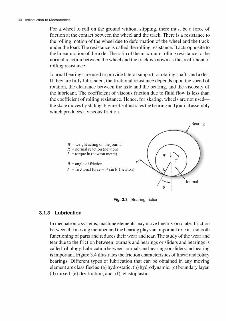
8/11/2019 Introduction to Mechatronics - Appuu Kuttan.pdf
http://slidepdf.com/reader/full/introduction-to-mechatronics-appuu-kuttanpdf 39/345
30 Introduction to Mechatronics
For a wheel to roll on the ground without slipping, there must be a force of
friction at the contact between the wheel and the track. There is a resistance to
the rolling motion of the wheel due to deformation of the wheel and the track
under the load. The resistance is called the rolling resistance. It acts opposite to
the linear motion of the axle. The ratio of the maximum rolling resistance to the
normal reaction between the wheel and the track is known as the coefficient of
rolling resistance.
Journal bearings are used to provide lateral support to rotating shafts and axles.
If they are fully lubricated, the frictional resistance depends upon the speed of
rotation, the clearance between the axle and the bearing, and the viscosity of
the lubricant. The coefficient of viscous friction due to fluid flow is less than
the coefficient of rolling resistance. Hence, for skating, wheels are not used—
the skate moves by sliding. Figure 3.3 illustrates the bearing and journal assembly
which produces a viscous friction.
W
R
T
Journal
F
q
Bearing
W
R
I
F W
= weight acting on the journal= normal reaction (newton)= torque in (newton metre)
= angle of friction
= frictional force = sin (newton)
q
q
Fig. 3.3 Bearing friction
3.1.3 Lubrication
In mechatronic systems, machine elements may move linearly or rotate. Frictionbetween the moving member and the bearing plays an important role in a smooth
functioning of parts and reduces their wear and tear. The study of the wear and
tear due to the friction between journals and bearings or sliders and bearings is
called tribology. Lubrication between journals and bearings or sliders and bearing
is important. Figure 3.4 illustrates the friction characteristics of linear and rotary
bearings. Different types of lubrication that can be obtained in any moving
element are classified as (a) hydrostatic, (b) hydrodynamic, (c) boundary layer,
(d) mixed (e) dry friction, and (f) elastoplastic.
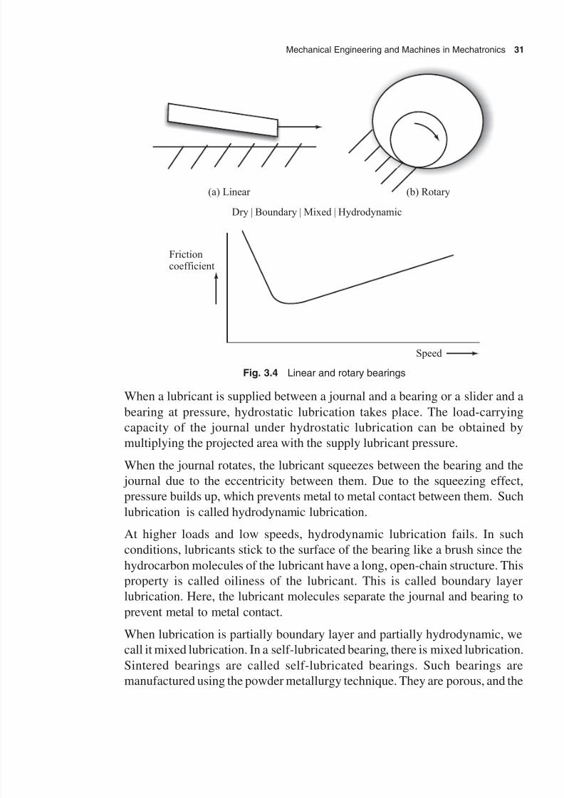
8/11/2019 Introduction to Mechatronics - Appuu Kuttan.pdf
http://slidepdf.com/reader/full/introduction-to-mechatronics-appuu-kuttanpdf 40/345
Mechanical Engineering and Machines in Mechatronics 31
(a) Linear (b) Rotary
Frictioncoefficient
Dry | Boundary | Mixed | Hydrodynamic
Speed
Fig. 3.4 Linear and rotary bearings
When a lubricant is supplied between a journal and a bearing or a slider and a
bearing at pressure, hydrostatic lubrication takes place. The load-carrying
capacity of the journal under hydrostatic lubrication can be obtained by
multiplying the projected area with the supply lubricant pressure.
When the journal rotates, the lubricant squeezes between the bearing and the
journal due to the eccentricity between them. Due to the squeezing effect,
pressure builds up, which prevents metal to metal contact between them. Such
lubrication is called hydrodynamic lubrication.
At higher loads and low speeds, hydrodynamic lubrication fails. In such
conditions, lubricants stick to the surface of the bearing like a brush since the
hydrocarbon molecules of the lubricant have a long, open-chain structure. This
property is called oiliness of the lubricant. This is called boundary layer
lubrication. Here, the lubricant molecules separate the journal and bearing to
prevent metal to metal contact.
When lubrication is partially boundary layer and partially hydrodynamic, we
call it mixed lubrication. In a self-lubricated bearing, there is mixed lubrication.
Sintered bearings are called self-lubricated bearings. Such bearings are
manufactured using the powder metallurgy technique. They are porous, and the

8/11/2019 Introduction to Mechatronics - Appuu Kuttan.pdf
http://slidepdf.com/reader/full/introduction-to-mechatronics-appuu-kuttanpdf 41/345
32 Introduction to Mechatronics
pores are filled with lubricants. At high speed, rotation of the journal causes a
rise in the surface temperature, which makes the lubricant to come to the surface
from the porous bearing due to capillary action. Thus, hydrodynamic lubrication
also can take place in sintered bearings.
When metal to metal contact takes place between the journal and bearing, dryfriction takes place. Dry friction is also called solid lubrication. Cast iron is a
good material for dry friction since nodular graphite spikes act as a good solid
lubricant.
An elastoplastic lubrication condition exists when a semisolid lubricant such as
grease or silica is used. In the elastoplastic lubricant, stress in the lubricant
linearly increases in small amounts with increase in strain. Grease used between
the gear teeth acts as the elastoplastic lubricant material, which prevents metal
to metal contact.
3.2 Behaviour of Materials Under Load
In this section, we will briefly study the behaviour of materials under load.
3.2.1 Stress and Strain
When an external force acts on a body, an internal resistance is set up within the
body to balance the external load. The resistance carried per unit area is called
the stress. When the applied force tends to compress the material or crush it, the
material is said to be in compression and the stress is referred to as compressivestress. When the force tends to expand the material or tear it apart, the material
is said to be in tension and the stress is referred to as tensile stress. When the
force tends to cause the particles of the material to slide over one another, the
material is said to be in shear stress. In the case of tensile force and compressive
force, the area carrying the force is the area of the cross section in the plane
perpendicular to the direction of the force. In the case of a shear force, the area
carrying the force is the area to be sheared in the direction of the line of action
of the force.
Figure 3.5 illustrates the different loading conditions on a rigid body. If a change
of motion of the rigid body is prevented, the force applied will cause a
deformation or change in the shape of the body. Strain is the change in dimension
that takes place in the material due to an externally applied force. Linear strain
is the ratio of change in length when a tensile or compressive force is applied.
Shear strain is measured by the angular distortion caused by an external force.
The load per unit deflection in a body is called stiffness. Deflection per unit
load is called compliance. If deformation per unit load at a point on the body is

8/11/2019 Introduction to Mechatronics - Appuu Kuttan.pdf
http://slidepdf.com/reader/full/introduction-to-mechatronics-appuu-kuttanpdf 42/345
Mechanical Engineering and Machines in Mechatronics 33
different from that at the point of application of the load then compliance at that
point is called cross compliance. In a machine structure cross compliance is an
important parameter for stability analysis during machining.
Fig. 3.5 A body in different loading conditions
3.2.2 Stress–Strain Behaviour
The strength of a material is expressed as the stress required to cause it to fracture.
The maximum force required to break a material divided by the original cross-
sectional area at the point of fracture is called the ultimate tensile strength of
the material in tension.
All materials are elastic to a certain extent. In the elastic region, the material
stretches if a tensile force is applied to it and returns to its original length on the
removal of the force. There is a limit to this elastic property in every material,
which is known as the elastic limit. If the force exceeds the elastic limit, thebody deforms. The stress corresponding to the elastic limit is called yield stress
The stress–strain curves for ductile and brittle materials are shown in Fig. 3.6.
When the material is loaded within the elastic limit, the stress is proportional to
strain. The constant of proportionality is called the modulus of elasticity or
Young’s modulus. Similarly, when shear stress is divided by shear strain, the
constant obtained is termed the modulus of rigidity.
It is obvious that the stress allowed in any component of a machine must be less
than the stress that would cause permanent deformation. A safe working stress

8/11/2019 Introduction to Mechatronics - Appuu Kuttan.pdf
http://slidepdf.com/reader/full/introduction-to-mechatronics-appuu-kuttanpdf 43/345
34 Introduction to Mechatronics
is chosen with regard to the conditions under which the material is to work. The
ratio of the yield stress to allowable stress is termed the factor of safety.
In the material machining operation, a number of parameters such as strain rate
and hardenability factor play an important role. Consider a thin plate of thickness
t , width b, and length l, subjected to tensile load P, which deforms by dl alongthe length, by db along the width, and by dt along the thickness. Then, stress s =
P / A, axial strain e a = dl / l, transverse strain e b = db / b, and the thickness strain e t= dt / t . Young’s modulus, E = stress/strain = s / e a, and Poisson’s ratio,
n = transverse strain/axial strain = – e b / e a . Poisson’s ratio for steel varies from
0.1 to 0.3. The ratio of thickness strain to axial strain (e t / e a) is called the r
parameter. Due to the conservation of mass, the volume of the material before
and after deformation is the same. Hence e a + e b + e c = 0 is used to determine e t .Parameters such as Young’s modulus, Poisson’s ratio, and r parameter are very
important properties of material in the context of mechatronic systems.
b
P
P
t
Elastic | plastic
Cup and cone Fracture
l
b
t
P
A
= length of the specimen= width of the specimen= thickness of the specimen= applied load= cross-sectional area
(a) (b)
Fig. 3.6 Stress–strain curves (a) ductile material and (b) brittle material
For isotropic materials, Young’s modulus E and Poisson’s ratio n are constants
along the x , y, and z directions. Steel, alloys, and non-ferrous metals behave like
isotropic materials. If Young’s modulus and Poisson’s ratio are different along
the x , y, and z directions, then the material is said to be anisotropic. Resins,
composites, metal matrix composites, and fibre reinforced plastic (FRP) are
examples of anisotropic materials. Metals and alloys have unique physical

8/11/2019 Introduction to Mechatronics - Appuu Kuttan.pdf
http://slidepdf.com/reader/full/introduction-to-mechatronics-appuu-kuttanpdf 44/345
Mechanical Engineering and Machines in Mechatronics 35
properties. Tailored physical properties can be obtained in composite form by
different orientations of fibres or reinforcement.
Figure 3.7 illustrates the stress–strain relationship of different materials under
different loading conditions. Materials may be ideal plastic or ideal elastic.
After the elastic limit, materials may behave as elastoplastic or visco-elastoplasticmaterials. Adhesive materials or brazed materials behave like elastoplastic
materials whereas materials at high temperature deform under visco-elasto-
plastic material model. Visco-elastoplastic material behaviour is a time-
dependent problem.
Strictly speaking, for elastic, elastoplastic, visco-elastoplastic, or brittle materials
in the elastic range, the stress–strain relationship is not linear. The non-linear
stress–strain relationship can be expressed as s = k e n, where k is called the
hardenability factor and n is the hardenability index. The hardenability factor
and hardenability index play an important role in the deformation behaviour of
elastoplastic or visco-elastoplastic materials.
Fig. 3.7 Stress–strain behaviour
3.2.3 Bending of Beams and Torsion on Shaft
The term ‘beam’ is used for a single rigid length of the material that can support
a system of external forces at right angles to its axis. A beam may be loaded
with a concentrated load or a distributed load, or both. A rigid, long material
that can carry axial loads only is called a strut.
A beam which is fixed at one end, leaving the other end free, is called a cantilever.
A beam with its ends resting freely on a support is called a simply supported
beam, and a beam with both ends fixed is called a fixed beam.

8/11/2019 Introduction to Mechatronics - Appuu Kuttan.pdf
http://slidepdf.com/reader/full/introduction-to-mechatronics-appuu-kuttanpdf 45/345
36 Introduction to Mechatronics
The loads on a beam tend to shear the beam and bend it as well. These effects
on the beam are measured by measuring the shearing force and bending moment,
respectively. The effect of a bending beam is to cause tensile and compressive
stresses in it. Tensile stresses are set up in the lower half of the section and
compressive stresses in the upper half. The axis with a stress value of zero is
called the neutral axis. The stress at any distance y from the neutral axis is given
by s t = E ( y / R), where E is Young’s modulus and R is the radius of curvature of
the neutral axis. The deflection of a beam at any point at a distance x is calculated
from the equation
d 2 y / dx
2= M / I = I / R
where M is the bending moment and I is the area inertia of the section. Combining
the governing equations, one can get the famous beam relation
M / I = E / R = s t / y
The moment of a force applied to a shaft which tends to twist or turn it is termedas turning moment or torque. The shaft suffers a shear stress. The shear stress at
any point in a cross section at a distance r from the axis of the shaft is given by
t = Gq r / L, where G is the modulus of rigidity, q is the angle of twist, and L is the
length of the shaft. When a torque, T , is applied to the shaft, it develops an
internal resistance and the resulting deflection can be calculated as q = TL / GJ ,
where J is the polar moment of inertia. Combining the governing torsion
equations, the torque relationship is obtained as T / J = Gq / L = t / r . Figure 3.8
illustrates the bending and torsion effects on materials.
Fig. 3.8 (a) Bending of beams and (b) torsion of shaft
3.2.4 Trusses and Frames
Structures composed of bar elements and those composed of beam elements
are classified as trusses and frames, respectively. Bars can only carry axial loads
and deform axially, whereas beams can take transverse loads and bending
moments about an axis perpendicular to the plane of the member. All the
members of a truss are subjected to only axial loads and a truss cannot carry
transverse shearing forces and bending moments.

8/11/2019 Introduction to Mechatronics - Appuu Kuttan.pdf
http://slidepdf.com/reader/full/introduction-to-mechatronics-appuu-kuttanpdf 46/345
Mechanical Engineering and Machines in Mechatronics 37
In a truss all the members are connected to each other through pins that allow
free rotation about the pin axis. On the other hand, in welded or riveted joints,
a number of frame elements are connected by rigid connectors, so that axial and
transverse forces and bending moments can be developed in the member. In
many truss-and-frame structures, the bar and beam elements are found in manydifferent orientations. Quantities such as displacement and forces for bar and
beam elements are shown in Fig. 3.9.
v2
P 2
u2
v1
2
1u1
P 1
u = deflection along the x direction, v = deflection along the y direction, and
P = axial load.
The axial deflection is resolved into components along the x and y directions.
(a) Bar element
v2 P 2
u2
v12
1
u1
P 1
F 2 P 2
2
1
P 1
F 1
M 1
M 2
Displacement vector Force vector
F M = shear force, = bending moment, and = slope.
(b) Beam element
1
2
Fig. 3.9 Displacement and forces in bar and beam elements

8/11/2019 Introduction to Mechatronics - Appuu Kuttan.pdf
http://slidepdf.com/reader/full/introduction-to-mechatronics-appuu-kuttanpdf 47/345
38 Introduction to Mechatronics
3.3 Materials
The modern mechatronic systems are designed to operate at higher speeds andfeeds. They should possess improved accuracy and higher rigidity, and shouldoperate at reduced noise levels. This calls for optimizing the design of
mechatronic system elements and selection of the right type of materials.Effective heat treatment and fabrication are of the utmost importance. The factorsto be considered while selecting the materials are: (a) functional requirement,(b) ease of fabrication, (c) machinability, (d) cost, and (e) availability.
Materials used for mechatronic systems are classified as (a) casting materialssuch as grey cast iron, spheroidal graphite cast iron, malleable cast iron, steelcasting, and casting of copper-based alloys and aluminium-based alloys, and(b) rolled or forged materials such as medium carbon-steel, alloy steel, high-
speed steels, forged copper-based alloys and aluminium-based alloys.
Miscellaneous materials such as friction-reducing materials turcite, plastic, andrubber products and metallic resins and fibre composites are widely used inmechatronic systems in industries.
3.4 Heat Treatment
Heat treatment is a process of austenite transformation into slow or fast coolingproducts by a diffusion or diffusionless process. Annealing refers to any heating,soaking, and cooling operation which is usually done to induce softening.Annealing may also be carried out to relieve internal stress induced by a cold or
hot working process. Normalizing is a process of heating steel to 50°C abovethe upper critical temperature followed by cooling in still air. The primarypurpose of normalizing is to refine the grain structure prior to hardening or toreduce segregation in casting or forging and to harden the steel slightly to improvemachinability.
Case hardening is a process of hardening ferrous alloys in which the surface
layer or case is made substantially harder than the interior or core. The hardersurface is resistant to wear and fatigue, and a toughened core resists impact andbending. Flame hardening is a process of case hardening wherein the surface ofthe metal is heated very rapidly by using an oxy-acetylene flame (thereby creatinga thermal gradient) and subsequently quenching in water or oil. Inductionhardening involves the case hardening of a ferrous alloy by heating it above the
transformation range by means of electrical induction and cooling as desired.Liquid carbursing involves the case hardening of low-carbon and alloy steelsby heating above the critical range in a molten cyanide salt, which induces bothcarbon and nitrogen into the case.
Nitriding is a process of case hardening of a special alloy steel in an atmosphereof ammonia or in contact with nitrogen material at a temperature below the
8/11/2019 Introduction to Mechatronics - Appuu Kuttan.pdf
http://slidepdf.com/reader/full/introduction-to-mechatronics-appuu-kuttanpdf 48/345
Mechanical Engineering and Machines in Mechatronics 39
transformation range. Surface hardness is caused by the absorption of nitrogenwithout quenching.
3.5 Electroplating
Electroplating or electrodeposition is a branch of electrometallurgy which dealswith the art of depositing metals by means of electric current. The mechanismof electroplating is based on the theory of ionic dissociation and electrolysis.Copper can be electroplated on both ferrous and non-ferrous metals by usingsolutions of copper cyanide or acids. Commercial electroplating generallyinvolves the use of copper cyanide, since more copper can be electroplated bythis method. Most nickel plating salts are a mixture of nickel sulphate and nickel
chloride, basic acid and stabilizers to control the quantity of nickel deposits.Chromium plating is done for decorative purposes, to improve corrosion
resistance or to produce hard, abrasion-resistant surfaces. Tin, cadmium, silver,and gold plating are commonly used in mechatronic systems in industries.
3.6 Fits and Tolerance
The relationship resulting from the difference between the sizes of two features,the hole and the shaft, is called fit. Fits have a common basic size. They are
broadly classified as clearance fit, transition fit, and interference fit. A clearancefit is one that always provides a clearance between the hole and shaft when theyare assembled. A transition fit is one that provides either a clearance or an
interference between the hole and the shaft when they are assembled. Aninterference fit is one that provides an interference all along between the holeand the shaft when they are assembled. There are two types of systems of fits—
(a) the hole-based system and (b) the shaft-based system.
In the hole-base system, the size of the hole is the basic size, denoted by H . Thesize of the shaft is varied to get the required fit. Letters a, b, c, d , e, f , and g
indicate loose fit, h, i, j, k and l indicate transition fit, and the rest (m, n, , z)indicate interference fit. Similarly, in the shaft-based system, the design size ofthe shaft is the basic size, denoted by h. The size of the hole is allowed to vary
according to the type of fit. A, B, C , D, E , F , and G indicate loose fit, H , I , J , K ,and L indicate transition fit, and the rest indicate interference fit. The hole-based system is generally used in industries. This is because a shaft is easy tomanufacture with a variety of sizes. The shaft-based system should only beused where there are definite economic advantages of doing so. For instance, inthe assembly of a piston inside a bored cylinder, boring of the cylinder is more
economical than changing the piston to get the correct fit.
The production of a part with exact dimensions repetitively is often difficult.
Hence, it is sufficient to produce parts with dimensions accurate within two
8/11/2019 Introduction to Mechatronics - Appuu Kuttan.pdf
http://slidepdf.com/reader/full/introduction-to-mechatronics-appuu-kuttanpdf 49/345
40 Introduction to Mechatronics
permissible limits of size. The difference in the limits of the size is called
tolerance. Tolerance can be provided on both sides of the basic size (bilateral
tolerance) or on one side of the basic size (unilateral tolerance). The ISO system
of tolerance provides for a total of 20 standard tolerance grades, which are
indicated as IT0, IT01, and IT1 to IT18.In any engineering industry the components manufactured should also satisfy
the geometrical tolerances in addition to the common dimensional tolerances.
Geometrical tolerances are classified as:
(a) Form tolerance—straightness, flatness, circularity, cylindricity, profile of
any line, and profile of any surface.
(b) Orientation tolerance—parallelism, perpendicularity, and angularity.
(c) Location tolerance—position, concentricity, co-axiality, and symmetry.
(d) Runout tolerance—circular runout and axial runout.
Geometrical tolerance should be specified only where it is essential. Geometrical
tolerance features are covered by ISO: 1101 – 1983.
3.7 Surface Texture and Scraping
Any surface, cylindrical or flat, has to be defined for the requirements of surface
roughness depending on its functional application to guarantee quality of
products. Surface roughness should not be specified if it is not required. It can
be measured and specified with different parameters such as the centre line
average (CLA) value Ra, ten-point average value R z, and maximum peak value
Rmax. The Ra value is the most commonly used international parameter for
roughness. It is defined as the arithmetic mean of the absolute values of the
profile departure within the sampling length. The roughness symbols, equivalent
roughness values, roughness grade numbers, and machining processes are given
in Table 3.1. Each quality class is established by the number of contact pairs
between the scraped surface and the inspection surface plate. The contact points
may be almost uniformly distributed in an area of 25 mm ¥ 25 mm and also
over the entire area of the scraped surface and checked by applying blue paste.
In the normal case, blue paste is applied to the masterpiece and the workpiece is
checked against it. For finer scraping, blue paste is used for the masterpiece and
a thin layer of red oxide mixed with linseed oil is used for the workpiece. The
red oxide gives a contrasting background and also prevents the blue paste from
spreading when the masterpiece is rubbed against the workpiece grades and the
various required parameters associate with them. Table 3.2 shows the various
scraped quality grades.

8/11/2019 Introduction to Mechatronics - Appuu Kuttan.pdf
http://slidepdf.com/reader/full/introduction-to-mechatronics-appuu-kuttanpdf 50/345
Mechanical Engineering and Machines in Mechatronics 41
Table 3.1 Roughness symbols and grades
Roughness Roughness Roughness
symbol value grade Machining process
R a (mm) number
~ — 50 N12 Casting, un-machined surface
— 25 N11
12.5 N10 Rough turning, planing, etc.
6.3 N9
—— 3.2 N8 Finish turning, milling, and drilling
1.6 N7
——— 0.8 N6
0.4 N5 Grinding, boring, and reaming0.2 N4
———— 0.1 N3
0.05 N2 Lapping, honing, etc.
0.025 N1
Table 3.2 Scraped quality grades and other parameters
Scraped Number of Surface Application
quality contact roughness grade points (mmmmmm)
1 22–32 0.1 Precision measuring machines,
instruments
2 15–21 0.2 Surface plates with straight edges,
guideways (machine tool slides)
3 10–14 0.4 Jigs and fixtures, guideways
(machine tools)
4 6–9 0.8 Surface tables, clamps
5 4–5 1.6 Rotary tables, covers of gear boxes
3.8 Machine Structure
The machine structure is the load carrying and supporting member of a machine
tool. Motors that drive mechanisms and other functional assemblies of the machine
tool are aligned to each other and rigidly fixed to the machine structure. Machine
structures are subjected to static and dynamic forces. It is therefore essential

8/11/2019 Introduction to Mechatronics - Appuu Kuttan.pdf
http://slidepdf.com/reader/full/introduction-to-mechatronics-appuu-kuttanpdf 51/345
42 Introduction to Mechatronics
that they do not deform or vibrate beyond the permissible limit under the action
of forces. The machine structure configuration is also influenced by
considerations of manufacture, assembly, and operation. The basic design factors
involved in the design of a machine tool structure are static load, dynamic load,
and thermal load. The static load of machine tools results from weights of slidesand the workpiece, and from the force due to cutting. The structure should have
adequate stiffness to keep the deformation of the structure within the permissible
value. Dynamic loads are often used for the constantly changing forces acting
on the structure while movement takes place. These forces may cause the whole
machine system to vibrate. The origins of such vibration are (a) unbalanced
rotating parts, (b) improper machine gears, (c) bearing irregularities, and (d)
interrupted cuts while machining.
In a machine tool, there are a number of local heat sources which set up thermal
gradients within the structure of the machine. Some of the heat sources are (a)
the electric motor, (b) friction in mechanical drives, (c) friction in bearings, (d)
the machining process, and (e) the temperature of the surrounding objects.
The heat sources cause localized deformation, resulting in considerable
inaccuracies in machine performance.
3.9 Guideways
Guideways are used in machine tools to control the direction or line of action of
the carriage or the table on which a tool or workpiece is held and to absorb allthe static and dynamic forces. The shapes and sizes of the workpieces produced
depend on the geometric and kinematic accuracy of the guideways. The
geometric relationship of the slide and guideways with the machine base
determines the geometric accuracy of the machine. Kinematic accuracy depends
on the straightness, flatness, and parallelism error in the guideways. Moreover,
any kind of wear in the guideways reduces the accuracy of the guide motion.
The points that must be considered while designing guideways are (a) rigidity,
(b) dampening capability, (c) geometric and kinematic accuracy, (d) velocity of
slide, (e) friction characteristic, (f) provision for adjustment of ply, (g) position
relative to work area, and (h) protection against swarf and damage.
Guideways are generally of two types—friction guideways and antifriction linear
motion guideways. Figure 3.10 illustrates different friction guideways.
Antifriction linear motion guideways are used in CNC machines and tools
because they (a) reduce the amount of wear, (b) improve smoothness of
movement, (c) reduce friction, (d) reduce heat generation.

8/11/2019 Introduction to Mechatronics - Appuu Kuttan.pdf
http://slidepdf.com/reader/full/introduction-to-mechatronics-appuu-kuttanpdf 52/345
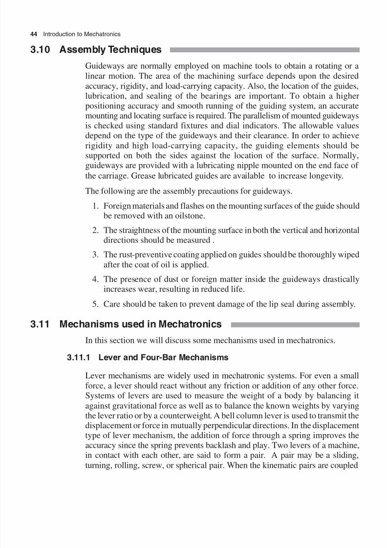
8/11/2019 Introduction to Mechatronics - Appuu Kuttan.pdf
http://slidepdf.com/reader/full/introduction-to-mechatronics-appuu-kuttanpdf 53/345
44 Introduction to Mechatronics
3.10 Assembly Techniques
Guideways are normally employed on machine tools to obtain a rotating or a
linear motion. The area of the machining surface depends upon the desired
accuracy, rigidity, and load-carrying capacity. Also, the location of the guides,
lubrication, and sealing of the bearings are important. To obtain a higherpositioning accuracy and smooth running of the guiding system, an accuratemounting and locating surface is required. The parallelism of mounted guidewaysis checked using standard fixtures and dial indicators. The allowable valuesdepend on the type of the guideways and their clearance. In order to achieve
rigidity and high load-carrying capacity, the guiding elements should besupported on both the sides against the location of the surface. Normally,guideways are provided with a lubricating nipple mounted on the end face of
the carriage. Grease lubricated guides are available to increase longevity.
The following are the assembly precautions for guideways.
1. Foreign materials and flashes on the mounting surfaces of the guide shouldbe removed with an oilstone.
2. The straightness of the mounting surface in both the vertical and horizontaldirections should be measured .
3. The rust-preventive coating applied on guides should be thoroughly wiped
after the coat of oil is applied.
4. The presence of dust or foreign matter inside the guideways drastically
increases wear, resulting in reduced life.
5. Care should be taken to prevent damage of the lip seal during assembly.
3.11 Mechanisms used in Mechatronics
In this section we will discuss some mechanisms used in mechatronics.
3.11.1 Lever and Four-Bar Mechanisms
Lever mechanisms are widely used in mechatronic systems. For even a small
force, a lever should react without any friction or addition of any other force.Systems of levers are used to measure the weight of a body by balancing it
against gravitational force as well as to balance the known weights by varyingthe lever ratio or by a counterweight. A bell column lever is used to transmit thedisplacement or force in mutually perpendicular directions. In the displacementtype of lever mechanism, the addition of force through a spring improves theaccuracy since the spring prevents backlash and play. Two levers of a machine,in contact with each other, are said to form a pair. A pair may be a sliding,
turning, rolling, screw, or spherical pair. When the kinematic pairs are coupled

8/11/2019 Introduction to Mechatronics - Appuu Kuttan.pdf
http://slidepdf.com/reader/full/introduction-to-mechatronics-appuu-kuttanpdf 54/345
Mechanical Engineering and Machines in Mechatronics 45
in such a way that the last link is joined to the first link to transmit definitemotion, they are said to form a kinematic chain. When any of the levers of thekinematic chain is fixed, the chain is known as a mechanism. A mechanism
with four levers is known as a four-bar mechanism. When a mechanism isrequired to transmit power or to do some particular type of work, it becomes a
machine. Obtaining different mechanisms by fixing different links in a kinematicchain is known as inversion of mechanism. Inversions of a four-bar chainmechanism are (a) crank-and-lever mechanism, (b) double-crank mechanism,and (c) double-lever mechanism.
Figure 3.12 illustrates the working of a simple lever and bell crank lever and
Fig. 3.13 shows the four-bar mechanism and its inversion.
F
A B
W
Lever ratio = / B A
(a) Simple lever (b) Bell column lever
Fig. 3.12 Simple and bell column levers
(a) Four-bar chain (b) Single-slider crank chain
(c) Double-slider crank chain (d) Double-lever mechanism
Fig. 3.13 Inversion of four-bar chain

8/11/2019 Introduction to Mechatronics - Appuu Kuttan.pdf
http://slidepdf.com/reader/full/introduction-to-mechatronics-appuu-kuttanpdf 55/345
46 Introduction to Mechatronics
3.11.2 Bearings
Mechanisms working on friction include the plane power screw, pivot and collar
beams, and friction clutches. When a body rests and is pulled by a traction
force, the limiting angle of friction, b = tan–1m , which is defined as the angle
that the resultant reaction force makes with the normal reaction force. Here m isthe friction coefficient. An inclined plane is used for many applications working
under friction. The body resting on the inclined plane may move down the
plane when a is greater than b , where a is the inclination of the inclined plane.
The screws used are power screws which work under the principle of the inclined
plane. The torque required to overcome the friction between the screw and nut
is T = w tana d /2, where w is the load on the bolt, a is the helix angle, and d is
the mean diameter of the screw. If b is less than a , the torque required to lower
the load will be negative. In other words, the load will start moving downwards
without the application of torque. Such a condition is known as overhauling of
the screws. If b is greater than a , the torque required to lower the load will be
positive, indicating that an effort is applied to lower the load. In such a case, the
screw is known as a self-locking screw. Figure 3.14 illustrates the friction effect
on an inclined plane. Rotating shafts are frequently subjected to axial thrust.
Bearing surfaces such as pivot and collar bearings are used to take the axial
thrust of the rotating shaft. Propeller shafts of ships, steam turbines, and
instruments with moving spindles are examples of shafts which carry an axial
thrust. Figure 3.15 shows the different pivot bearings and a single flat collar
bearing.
W
P W
(a) Limiting angle of friction (b) Angle of response of inclined plane
R N
F W = sin a F R= m N
Fig. 3.14 Friction and inclined plane
Fig. 3.15 Pivot bearings and single flat collar

8/11/2019 Introduction to Mechatronics - Appuu Kuttan.pdf
http://slidepdf.com/reader/full/introduction-to-mechatronics-appuu-kuttanpdf 56/345
Mechanical Engineering and Machines in Mechatronics 47
A rolling element bearing is considered a very important mechanical component
as it is used for almost all rotary applications. Such a bearing consists of two
circular metal rings and a set of rolling elements. One of the rings is larger than
the other. The smaller of the two is called the inner ring and the larger one the
outer ring. The inner ring fits well within the perimeter of the outer ring. Figure3.16 shows a typical roller bearing. All the bearing parts are in transition fit
since the bearing should allow a free rotation of the rolling element and the
outer and inner rings should not get cold welded with the housing or body.
Bearings have to deal with radial and thrust loads. For this purpose, different
rolling elements such as balls, cylindrical rollers, and needle type or tapered
rollers are used.
Fig. 3.16 Roller bearings
Mechanical friction losses are eliminated in magnetic bearings. Figure 3.17
shows a typical magnetic bearing. Electromagnetic bearings are used for journal
suspension in magnetic bearings. Magnetic bearings are used for high-speed
application and also where more accurate positioning is essential.
Electromagnet
F W F
F
F
W
= += upward force due to top electromagnet= downwards force due to bottom electromagnet= weight of the rotor
1
1
W
F 1
Rotor
F
Fig. 3.17 A magnetic bearing

8/11/2019 Introduction to Mechatronics - Appuu Kuttan.pdf
http://slidepdf.com/reader/full/introduction-to-mechatronics-appuu-kuttanpdf 57/345
48 Introduction to Mechatronics
Bearings are an integral part of nanomechanisms. Molecular bearings are likely
to be used in the function of molecular machines. This type of bearing does not
require lubrication.
3.11.3 Clutches
The principal application of the friction clutch is in the transmission of power
of shafts and machines which must be started and stopped frequently. The force
of friction is used to start the shaft from rest and gradually bring it up to the
proper speed without excessive slippage of the friction surface. In an automobile,
the friction clutch is used to connect the engine to the driven shaft. Friction
clutches of different types such as disc or plate clutch (single disc or multiple
disc clutch), cone clutch, and centrifugal clutch are commonly used.
The cone clutch consists of a pair of friction surfaces only. The contact surfacesof the clutch may be metal to metal, but more often the driven member is lined
with some material such as wood, leather, cork, or asbestos. Figure 3.18 shows
a cone clutch.
Drive Driven
Fig. 3.18 A cone clutch
Centrifugal clutches are usually incorporated into motor pulleys. Such a clutch
consists of a number of shoes on the inside of a rim of the pulley, as shown in
Figure 3.19. The outer surfaces of the shoes are covered with friction material.
These shoes, which can move radially in the guide, are held against a spider on
the driving shaft by means of a spring. The spring exerts a radially inward force,
which is assumed constant. The mass of the shoes when revolving causes a
radially inward force (centrifugal force). The magnitude of the centrifugal force
depends on the speed. When this force exceeds the spring force, the shoe moves
outwards and comes into contact with the driven member and thus transmits
power.
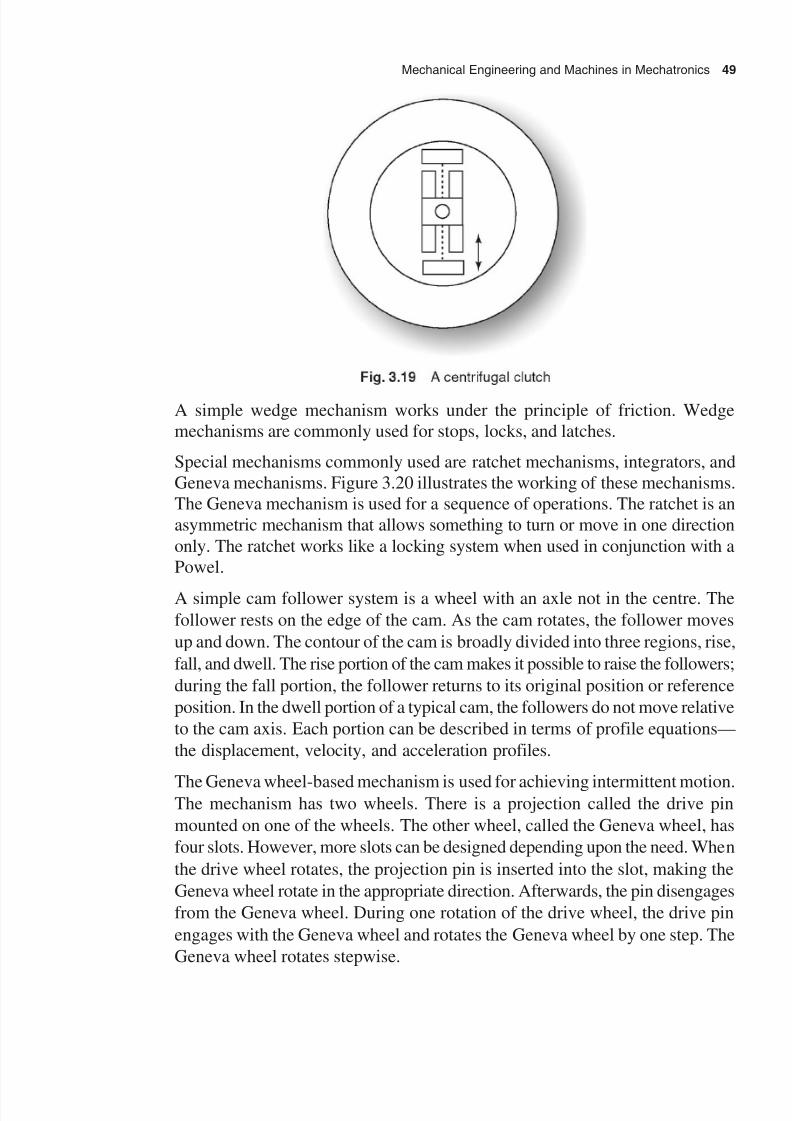
8/11/2019 Introduction to Mechatronics - Appuu Kuttan.pdf
http://slidepdf.com/reader/full/introduction-to-mechatronics-appuu-kuttanpdf 58/345
Mechanical Engineering and Machines in Mechatronics 49
Fig. 3.19 A centrifugal clutch
A simple wedge mechanism works under the principle of friction. Wedge
mechanisms are commonly used for stops, locks, and latches.
Special mechanisms commonly used are ratchet mechanisms, integrators, and
Geneva mechanisms. Figure 3.20 illustrates the working of these mechanisms.
The Geneva mechanism is used for a sequence of operations. The ratchet is an
asymmetric mechanism that allows something to turn or move in one direction
only. The ratchet works like a locking system when used in conjunction with a
Powel.
A simple cam follower system is a wheel with an axle not in the centre. The
follower rests on the edge of the cam. As the cam rotates, the follower moves
up and down. The contour of the cam is broadly divided into three regions, rise,
fall, and dwell. The rise portion of the cam makes it possible to raise the followers;
during the fall portion, the follower returns to its original position or reference
position. In the dwell portion of a typical cam, the followers do not move relative
to the cam axis. Each portion can be described in terms of profile equations—
the displacement, velocity, and acceleration profiles.
The Geneva wheel-based mechanism is used for achieving intermittent motion.The mechanism has two wheels. There is a projection called the drive pin
mounted on one of the wheels. The other wheel, called the Geneva wheel, has
four slots. However, more slots can be designed depending upon the need. When
the drive wheel rotates, the projection pin is inserted into the slot, making the
Geneva wheel rotate in the appropriate direction. Afterwards, the pin disengages
from the Geneva wheel. During one rotation of the drive wheel, the drive pin
engages with the Geneva wheel and rotates the Geneva wheel by one step. The
Geneva wheel rotates stepwise.

8/11/2019 Introduction to Mechatronics - Appuu Kuttan.pdf
http://slidepdf.com/reader/full/introduction-to-mechatronics-appuu-kuttanpdf 59/345
50 Introduction to Mechatronics
Gear trains are mechanisms used in almost all machines to facilitate the
transmission of power and motion. They help increase or decrease torque or
speed, and can change the direction of the axis of rotation. Depending upon the
teeth, gears are grouped as (a) spur gears, (b) bevel gears, (c) helical gears, and
(d) worm gears.
(a) Wedge mechanism
(c) Linear ratchet
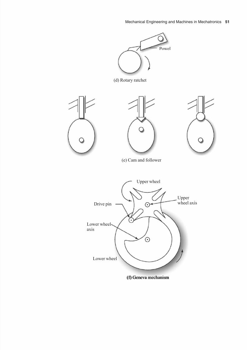
8/11/2019 Introduction to Mechatronics - Appuu Kuttan.pdf
http://slidepdf.com/reader/full/introduction-to-mechatronics-appuu-kuttanpdf 60/345
Drive pin
Upper wheel axis
Lower wheelaxis
Lower wheel
(f) Geneva mechanism
Upper wheel
Mechanical Engineering and Machines in Mechatronics 51
(d) Rotary ratchet
Powel
(e) Cam and follower

8/11/2019 Introduction to Mechatronics - Appuu Kuttan.pdf
http://slidepdf.com/reader/full/introduction-to-mechatronics-appuu-kuttanpdf 61/345
52 Introduction to Mechatronics
(g) Gear train (h) Rack and pinion
Fig. 3.20 Special mechanisms used in mechatronics
The number of teeth, diameter, and rotating velocity are extremely important in
the context of gears. If one gear has 120 teeth and another has 20 teeth, the gear
ratio is 6:1. The gear ratio indicates the ratio of speeds. Pitch diameter divided
by the number of teeth is called the module of a gear. Two gears can mate if
their modules are the same.The rack-and-pinion drive mechanism is a special type of gear mechanism in
which rotary motion in converted into linear motion and vice versa. It consists
of a rack and pinion. The rack is a long, flat piece of metal. The flat side contains
teeth running throughout the length of the rack. The teeth are perpendicular to
the edge of the rack. The pinion is like a gear that also has teeth on it. These
teeth run parallel to the length of the shaft. The pinion has rotary motion, whereas
the rack gives linear motion just like any gear train. A rack and pinion is
lubricated in order to minimize wear.
Illustrative Examples
Example 3.1 A load of 5 kN is to be raised with the help of a steel wire. Find
the minimum diameter of the wire if the stress is not to exceed 100 mN/m2.
Solution
Load P = 5 kN
Induced stress s = 100 ¥ 10 6 N/m2
If the diameter of the wire is D,
cross-section area A = p D2
4
Then,
P / A = 100 ¥ 106
Solving,
D = 0.0079 m = 7.97 mm

8/11/2019 Introduction to Mechatronics - Appuu Kuttan.pdf
http://slidepdf.com/reader/full/introduction-to-mechatronics-appuu-kuttanpdf 62/345
Mechanical Engineering and Machines in Mechatronics 53
Example 3.2 A steel bar of diameter 20 mm and length 20 cm was tested to
destruction. The load at the elastic limit is 65 N and the corresponding extension
is 0.22 mm. Determine the modulus of elasticity and the strain at the elastic
limit.
Solution
Diameter of the bar = 20 mm
Length of the bar = 20 cm
Elongation at elastic limit = 0.22 mm
Load at elastic limit = 65 kN
Stress = load / area = P / A = 0.2069 kN/m2
Strain at elastic limit = extension at elastic limit/original length
= 0.22/200 = 0.0011Modulus of elasticity = stress/strain
= 188.09 kN/mm2
Example 3.3 A steel plate 12 mm thick is bent around a drum. If the maximum
stress induced in the plate due to bending is 400 N/mm2, find the radius of the
drum. Take E = 2 ¥ 105 N/mm
2.
Solution
Thickness of the steel plate = 12 mm
Maximum stress s = 400 N/mm2
Modulus of elasticity E = 2 ¥ 105 N/mm
2
If R 1 is the radius of the drum and r is the radius of curvature of the neutral axis
of the plate, then
R = R1 + (12/2)
= R1 + 6
Using the equation for a beam,
s / y = E / R400/6 = 2 ¥ 105 / R
Solving,
R = 3000 mm
R1 = 2994 mm
Example 3.4 A simply supported beam 4 m long carries a point load of 50 kN
at a distance of 1.5 m from each end. If the allowable bending stress is 15.34
kN/cm2, find the section modulus.

8/11/2019 Introduction to Mechatronics - Appuu Kuttan.pdf
http://slidepdf.com/reader/full/introduction-to-mechatronics-appuu-kuttanpdf 63/345
54 Introduction to Mechatronics
Solution
The beam is symmetrically loaded. Hence, the reaction force on each support,
R = 50 kN. Bending moment at midspan where the maximum bending moment
occurs,
M max = R ¥ 2 – 50 ¥ 0.5 = 75 kN m
Using the beam equation,
M/I = s / Y
Z = I/Y = 488.92 cm2
Example 3.5 Find the maximum shearing stress developed in a shaft of 40
mm diameter when a twisting moment of 100 kN cm is applied. Also find the
cycle of twist in a length of 2 m of shaft. Take G = 8 ¥ 106 N/cm
2.
Solution
Diameter of the shaft d = 40 mm
Torque applied T = 100 kN cm
Length of the shaft = 200 cm
Modulus of rigidity G = 8 ¥ 106
N/cm2
Using the torque equation T/J = Gq / = 2s /d ,
T =p s
32
4d d
Solving,
s = 7957.7 N/cm2
Angle of twist
q =33 10 200
8 10 10
5
6 4
¥ ¥
¥ ¥p = 0.099 rad = 5.699°
Example 3.6 A conical friction clutch used for a mechatronic system transmits
90 kW at 1500 RPM. The semi-cone angle is 20° and the coefficient of friction
is 0.2. If the mean diameter of the beam surface is 375 mm and the intensity of
normal pressure is not to exceed 0.25 N/mm2, find the dimensions of the conical
clutch.
Solution
Power transmitted P = 90 kW = 90 ¥ 103 W
Speed of the drive shaft N = 1500 rpm
Cone angle a = 20°

8/11/2019 Introduction to Mechatronics - Appuu Kuttan.pdf
http://slidepdf.com/reader/full/introduction-to-mechatronics-appuu-kuttanpdf 64/345
Mechanical Engineering and Machines in Mechatronics 55
Friction coefficient m = 0.2
Mean diameter D = 375 mm
Normal pressure p = 0.25 N/mm2
Angular velocity w = 260p N = 156 rad
Mean radius R = D
2= 187.5 mm
Power transmitted = torque multiplied by angular velocity
Torque = 5.77 103 N mm
When the clutch is engaged,
Torque transmitted to driven pulley = 2p Rb = m pR
Hence,
Width of the clutch, b = 52.2 mm
Let the inside radius of the cone be r 1 and the outside radius r 2. Then
r 1 + r 2 = 2 R = 375
and r 1 – r 2 = b sin a = 18
Solving,
r 1 = 196.5 mm
and r 2 = 178.5 mm
Example 3.7 A centrifugal clutch has four shoes which slide in a spider
keyway. Each shoe has clearance of 5 mm between shoe and rim. The pull
exerted by the spring is 500 N. The mass centre of the shoe is 160 mm from the
axis of the clutch. If the internal diameter of the rim is 400 mm, the mass of
each shoe is 8 kg, the stiffness of the each spring is 50 N mm, and the coefficient
of friction between shoe and rim is 0.3, find the power transmitted by the clutch
at 500 rpm.
Solution
Number of shoes n = 4
Clearance between shoe and rim c = 5 mm
Spring pull when the clutch is at rest S = 500 N
Mass centre of the shoe r = 160 mm
Spring stiffness s = 50 N/mm
8/11/2019 Introduction to Mechatronics - Appuu Kuttan.pdf
http://slidepdf.com/reader/full/introduction-to-mechatronics-appuu-kuttanpdf 65/345
56 Introduction to Mechatronics
Friction coefficient m = 0.3
Speed of the drive shaft N = 500 rpm
Angular velocity w =2
60
p N = 52.37 rad/sec
Operating radius r 1 = r + c = 165 mm
Centrifugal force P f = mw 2r 1 = 3620 N
Upward force exerted by the spring,
Ps = initial pulling force + clearance multiplied by stiffness
= S + cs = 750 N
Friction force acting tangential on each shoe,
F f = m ( P f – Ps) = 861 N
Torque transmitted T = n F f R = 688.8 N
Power transmitted = Tw = 36.1 kW
Exercises
3.1 Define the terms stiffness, compliance, and cross compliance.
3.2 Discuss the different types of lubricating systems.
3.3 Explain the functions of self-lubricating bearings.
3.4 Define the terms hardenability factor, hardenability index, and r parameter.
3.5 Differentiate between trusses and frames.
3.6 Why is heat treatment required? Discuss double tempering treatment.
3.7 Differentiate between
(i) unilateral and bidirectional tolerances
(ii) the shaft-based system and the hole-based system.
3.8 Why do we need to scrape the surface of a machine tool? How is it done?3.9 Discuss the simple mechanisms used in mechatronic systems.
8/11/2019 Introduction to Mechatronics - Appuu Kuttan.pdf
http://slidepdf.com/reader/full/introduction-to-mechatronics-appuu-kuttanpdf 66/345
Electronics in Mechatronics
4.1 Conductors, Insulators, and Semiconductors
According to the definition given by the Institute of Electronics and Electrical
Engineers, USA, electronics is the science and technology of passage of charged
particles in gases, vacuum, or in semiconductors. Electricity flows in electric
motors, incandescent lamps, electric furnaces, and transformers through copper
wires or some metallic parts. The fluorescent lamp can be considered as an
electronic device as electrons flow in space from one end of the tube to the
other, whereas the common incandescent lamp cannot be considered as an
electronic device since current flows through the filament in it. The followingare the salient features of an electronic device.
1. It can respond to very small control signal.
2. It can respond at a speed far beyond the speed at which mechanical or
electrical devices can.
3. It is photosensitive.
4. It can rectify alternate current into direct current.
5. Some electronic devices can produce x-ray radiations.
To understand why some materials behave as conductors, insulators, or
semiconductors, the atomic structure of materials has to be understood. All
matter is made up of atoms consisting of a nucleus of positive charge. Negatively
charged electrons revolve around the nucleus in specific orbits. The positive
and negative charges form a strong bond and atoms become stable. As per the
Pauli’s exclusion principle, when the number of electrons in each orbit of an
atom is 2n2, where n is the orbit number, the atom becomes very stable. Hence,
in stable atoms such as those of halogens, the first orbit has two electrons and

8/11/2019 Introduction to Mechatronics - Appuu Kuttan.pdf
http://slidepdf.com/reader/full/introduction-to-mechatronics-appuu-kuttanpdf 67/345
58 Introduction to Mechatronics
the second has eight. The electrons in the outermost orbit are called valence
electrons and the outermost orbit itself is called valence orbit. In some materials,
stable atoms are obtained by sharing or donating the electrons. Accordingly, the
bond formed may be called an ionic bond or a covalent bond. Free electrons are
not available in such materials which act as insulators. Insulators cannot conductthermal energy or electricity. In metallic bonds, the outer valence electrons form
an electron cloud or gas and move around the material exhibiting Brownian
motion. Hence, metals are good conductors of electricity and thermal energy. In
the case of semiconductors the energy requirement is in between that of metals
and insulators. Hence, they behave as semiconductors of electricity. Graphite,
silicon, and germanium are examples of semiconductors.
Electrons not only revolve around the nucleus but also spin on their own axes.
If there are two electrons in an orbit, one electron rotates clockwise and the
other rotates anticlockwise. This produces a neutral momentum. In somematerials, there is positive momentum, indicating more clockwise spin. Such
materials are called paramagnetic materials. If there is a net negative momentum,
the material is said to be ferromagnetic.
4.2 Passive Electrical Components
Energy is classified into potential energy and kinetic energy. A body raised
above the ground level has a certain amount of potential energy. Similarly, the
voltage or electric potential at a point in an electric field can be defined as thework done in bringing one coulomb of positive charge to that point from infinity
against the electric field. Voltage is measured in volts. If the work done is 1 J,
then the potential at that point is 1 V. An electric current may be defined as the
movement of electric charge along a definite path. The current corresponding
to the flow of 1 C of charge per second through a conductor is 1 A. One ampere
of current is the flow of 6.24 ¥ 1018
electrons per second through a conductor. A
current in a conductor produces heating effect, magnetic field, and chemical
transformation when passed through a certain solution. The heating effect is
made use of in incandescent lamps, electric heaters, and furnaces. The magneticeffect is used in electromagnets and the chemical effect in electroplating.
Direct current (DC) is a unidirectional current which does not change its value
appreciably. The DC voltage is a unidirectional voltage like that of a battery. In
alternating current or voltage, the circuit direction of current or voltage reverses
at regular intervals of time. The sine wave is most frequently used in alternating
current or voltage. In this waveform, voltage or current varies from zero to a
positive peak, falls back to zero, reaches to a negative peak, and again comes
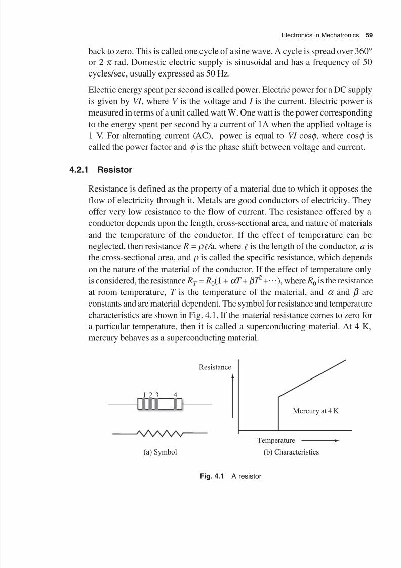
8/11/2019 Introduction to Mechatronics - Appuu Kuttan.pdf
http://slidepdf.com/reader/full/introduction-to-mechatronics-appuu-kuttanpdf 68/345
Electronics in Mechatronics 59
back to zero. This is called one cycle of a sine wave. A cycle is spread over 360°
or 2 p rad. Domestic electric supply is sinusoidal and has a frequency of 50
cycles/sec, usually expressed as 50 Hz.
Electric energy spent per second is called power. Electric power for a DC supply
is given by VI , where V is the voltage and I is the current. Electric power ismeasured in terms of a unit called watt W. One watt is the power corresponding
to the energy spent per second by a current of 1A when the applied voltage is
1 V. For alternating current (AC), power is equal to VI cosf , where cosf is
called the power factor and f is the phase shift between voltage and current.
4.2.1 Resistor
Resistance is defined as the property of a material due to which it opposes the
flow of electricity through it. Metals are good conductors of electricity. Theyoffer very low resistance to the flow of current. The resistance offered by a
conductor depends upon the length, cross-sectional area, and nature of materials
and the temperature of the conductor. If the effect of temperature can be
neglected, then resistance R = r / a, where is the length of the conductor, a is
the cross-sectional area, and r is called the specific resistance, which depends
on the nature of the material of the conductor. If the effect of temperature only
is considered, the resistance RT = R0(1 +a T + b T 2 +…), where R0 is the resistance
at room temperature, T is the temperature of the material, and a and b are
constants and are material dependent. The symbol for resistance and temperature
characteristics are shown in Fig. 4.1. If the material resistance comes to zero for
a particular temperature, then it is called a superconducting material. At 4 K,
mercury behaves as a superconducting material.
1 2 3 4
Resistance
Mercury at 4 K
Temperature
(a) Symbol (b) Characteristics
Fig. 4.1 A resistor

8/11/2019 Introduction to Mechatronics - Appuu Kuttan.pdf
http://slidepdf.com/reader/full/introduction-to-mechatronics-appuu-kuttanpdf 69/345
60 Introduction to Mechatronics
The resistances of some resistors are indicated by numbers. This method is used
for low value resistors. Most resistors are coded using colour bands. The first
band gives the resistance value of the resistor in ohms. The fourth band, which is
far away from the usual band, indicates the accuracy of the value. Red in this
region indicates 2%, gold indicates 5%, and silver indicates 10% accuracy. Table
4.1 indicates the colour codes, bands, and the corresponding resistance values.
Usually a resistor is made up of a film of carbon or a coil of nichrome wire.
Resistors are available in some standard values, power ratings, and tolerance
ranges. A nichrome wire has 75% Ni and 25% Cr. Its resistance does not vary
more than by 0.005 for a temperature change from 25°C to 125°C. The linearity
of the wire wound resistor is within 0.003%. Cermets are used as resistors.
Cermets are an abbreviation for ceramic metal. They consist of fine particles of
precious metals. They are manufactured by baking in kilns. Ceramic substrates
such as aluminium and sterlite are also used. Plastic conductors are made of
epoxy, polyester, and other resins blended with carbon powder to make themconductive. Their linearity can be held to 0.025%. When resistors are connected
end to end, they are said to be connected in series. The equivalent resistance is
equal to the sum of the individual resistances so connected. Resistors are said to
be connected in parallel if two or more resistors are connected across each
other. The equivalent resistance is equal to multiplication of the individual
resistances divided by the sum of individual resistances so connected.
Table 4.1 Colour and resistance value
Colour Band 1 Band 2 Band 3
Black 0 0
Brown 1 1 0
Red 2 2 0 0
Orange 3 3 0 0 0
Yellow 4 4 0 0 0 0
Green 5 5 0 0 0 0 0
Blue 6 6 0 0 0 0 0 0
Violet 7 7 0 0 0 0 0 0 0Grey 8 8 0 0 0 0 0 0 0 0
White 9 9 0 0 0 0 0 0 0 0 0
A potential divider is used for variable voltage supply and also as multiplier ofa fraction. Figure 4.2 shows the symbol of a potential divider and the diagram
of a wire wound circular potentiometer. Two potentiometers connected in parallelform a Wheatstone bridge circuit, which can be used as a transducer to convert
two mechanical inputs into an electrical signal. Refer to Fig. 4.2(c).

8/11/2019 Introduction to Mechatronics - Appuu Kuttan.pdf
http://slidepdf.com/reader/full/introduction-to-mechatronics-appuu-kuttanpdf 70/345
Electronics in Mechatronics 61
E i E
o
E
E
E KE K
= input voltage= output voltage
= for < 1
i
o
o i
Symbol
(a) Potential divider
E o
E i
Resistance
Resolution
ThresholdResolution = / D A
(b) Circular potentiometer
where is the diameter of the core, is the cross-sectional area of the wire,
and is the specific resistance.
D A
R1 R2
i
R4 R3
Error signal
When the bridgeis balanced,
R1 R3
R2 R4or
R1 R2
R3 R4
i = angular input
= angular output from a
mechanical system
(c) Conversion of two mechanical signals
Fig. 4.2 Potentiometer
4.2.2 Capacitor
A capacitor essentially consists of two conducting surfaces separated by a layer
of insulating medium called dielectric. The dielectric is an insulating mediumthrough which an electrostatic field can pass. The main purpose of the capacitor
is to store electrical energy. The property of the capacitor by which it stores
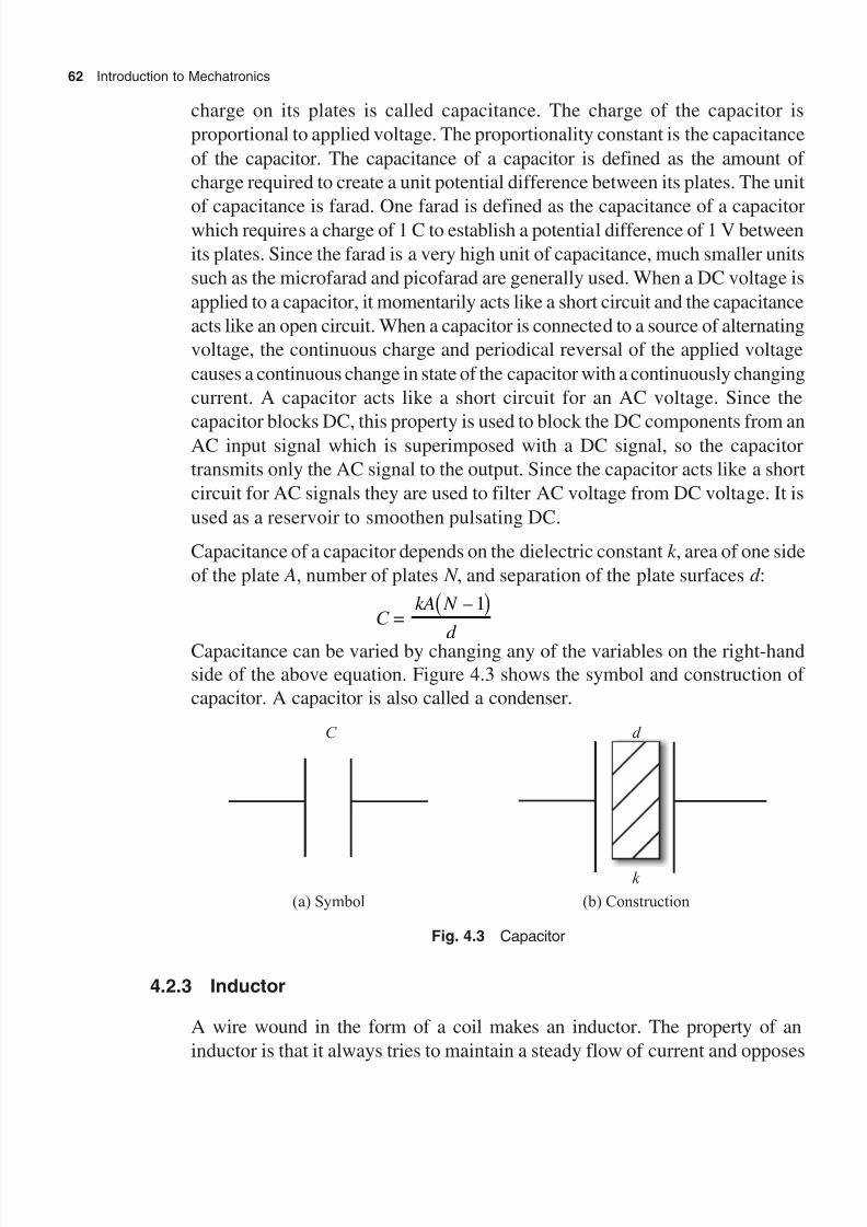
8/11/2019 Introduction to Mechatronics - Appuu Kuttan.pdf
http://slidepdf.com/reader/full/introduction-to-mechatronics-appuu-kuttanpdf 71/345
62 Introduction to Mechatronics
charge on its plates is called capacitance. The charge of the capacitor is
proportional to applied voltage. The proportionality constant is the capacitance
of the capacitor. The capacitance of a capacitor is defined as the amount of
charge required to create a unit potential difference between its plates. The unit
of capacitance is farad. One farad is defined as the capacitance of a capacitorwhich requires a charge of 1 C to establish a potential difference of 1 V between
its plates. Since the farad is a very high unit of capacitance, much smaller units
such as the microfarad and picofarad are generally used. When a DC voltage is
applied to a capacitor, it momentarily acts like a short circuit and the capacitance
acts like an open circuit. When a capacitor is connected to a source of alternating
voltage, the continuous charge and periodical reversal of the applied voltage
causes a continuous change in state of the capacitor with a continuously changing
current. A capacitor acts like a short circuit for an AC voltage. Since the
capacitor blocks DC, this property is used to block the DC components from anAC input signal which is superimposed with a DC signal, so the capacitor
transmits only the AC signal to the output. Since the capacitor acts like a short
circuit for AC signals they are used to filter AC voltage from DC voltage. It is
used as a reservoir to smoothen pulsating DC.
Capacitance of a capacitor depends on the dielectric constant k , area of one side
of the plate A, number of plates N , and separation of the plate surfaces d :
C =kA N
d
– 1
Capacitance can be varied by changing any of the variables on the right-handside of the above equation. Figure 4.3 shows the symbol and construction of
capacitor. A capacitor is also called a condenser.
(a) Symbol (b) Construction
k
d C
Fig. 4.3 Capacitor
4.2.3 Inductor
A wire wound in the form of a coil makes an inductor. The property of an
inductor is that it always tries to maintain a steady flow of current and opposes

8/11/2019 Introduction to Mechatronics - Appuu Kuttan.pdf
http://slidepdf.com/reader/full/introduction-to-mechatronics-appuu-kuttanpdf 72/345
Electronics in Mechatronics 63
any fluctuation in it. When a current flows through a conductor, it produces a
magnetic field around it in a plane perpendicular to the conductor. When a
conductor moves in a magnetic field, an electromagnetic force is induced in the
conductor. Imagine a coil of wire in a case connected to a battery. Whenever an
effort is made to increase the current through the coil, it is opposed by theinstantaneous production of a counter emf. The energy required to overcome
this opposition is supplied by the battery. This energy is stored in the inductor in
the form of additional magnetic flux produced. At this stage, if an effort is made
to decrease the current through the coil, the current decrease is delayed due to
the production of self-induced emf. The property of the inductor due to which it
opposes any increase or decrease in current by the production of a counter emf
is known as self-inductance. It is initially difficult to establish a current through
a coil, but once it is established it is equally difficult to withdraw it. Hence
inductance is sometimes called electrical inertia. The emf developed isproportional to the rate of current through the inductor. Mathematically, e =
LdI / dt , where the proportionality constant L is called the self-inductance of the
coil, I is the current, and e is the voltage developed.
Mutual inductance arrangements use two coils—one acting as the power coil
and the other as the supply output. A mutual inductance profile is used as a
sensor for measuring small displacements. A linear variable differential
transformer (LVDT) works under the principle of mutual inductance. Figure
4.4 illustrates the working of an inductor.
V , E i o
V i E o
V E
i
o= Input ac voltage= output inductance change(a) Self-inductance (b) Mutual inductance
Fig. 4.4 Inductor
Ohm’s law V = IR, where V is the supply voltage, I is the current, and R is the
resistance, holds good for DC supply. However, it cannot be used for AC supply
because of the current and voltage phase relationship. Impedance is defined as
AC resistance equal to the ratio of the voltage to the current. When a circuit
consists of several elements—resistances, capacitances, and inductances in series

8/11/2019 Introduction to Mechatronics - Appuu Kuttan.pdf
http://slidepdf.com/reader/full/introduction-to-mechatronics-appuu-kuttanpdf 73/345
64 Introduction to Mechatronics
or parallel, the resulting impedance can be calculated. Table 4.2 shows the various
formulae that can be used to calculate impedance. The impedance of a capacitor
is known as capacitive reactance and the impedance due to an inductor is knownas inductive reactance. The inductive reactance X L of an inductance is given by
Lw , where w = 2p f and f is the frequency. The capacitive reactance X C of acapacitor is given by X C = 1/ w C . Inductive reactance is positive, whereas
capacitive reactance is negative.
Table 4.2 Impedance formulae
Circuit Impedance
R
j w L
– j / w C
R + j w L
R – j / w C
R / (1+ j w CR )
R + j (w L – 1/ w C )
1
2 2 2
R j L
R L j C
– w
w w
++
4.2.4 Transformer
A transformer is a device by means of which electric power in one circuit istransferred to the another circuit without a change in frequency. It essentiallyconsists of two or more inductive windings wound on the same core. A transformercan raise or lower the voltage in a circuit with corresponding decrease or increasein current. Transformers are effectively used to step up and step down voltages inpower stations and substations, respectively, so that power losses can be minimized.
Figure 4.5 shows the schematic diagram of a transformer.

8/11/2019 Introduction to Mechatronics - Appuu Kuttan.pdf
http://slidepdf.com/reader/full/introduction-to-mechatronics-appuu-kuttanpdf 74/345
Electronics in Mechatronics 65
V
V
V I V I V N V N
I
N
1 = primary voltage= secondary voltage
= and == current= number of turns
2
1 1 2 2 1 1 2 2
V 2
V 1
Fig. 4.5 A transformer
4.3 Active Elements
Active elements have an auxiliary source of power which supplies a major part
of the output power while input signals supply only an insignificant portion.
There may or may not be a conversion of energy from one form to another.
Solenoid drives, electronic amplifiers, servosystems, and digital systems are
some examples of active devices.
4.3.1 Semiconductor Devices
Graphite, silicon, and germanium are semiconductor materials. Most commonly
Ge and Si are used in semiconductor devices. Silicon and germanium are
tetravalent, having four electrons in the outermost orbit. Both the materials are
crystalline in nature. At very low temperatures, say 0°C, the crystal behaves
like an insulator as there are no free electrons available in it. However, as the
temperature increases and reaches room temperature, some of the covalent bonds
are broken because of thermal energy, and the conductivity of the crystal
improves. The space where the electron can be accepted is called a hole. Eventhough pure silicon and germanium have free electrons and holes at room
temperature, conductivity is poor because the number of free electrons and holes
is not sufficient. In order to improve the conductivity of these materials, some
impurities are intentionally added. This addition of impurities in a semiconductor
is known as doping. Usually either pentavalent impurities such as phosphorous
and antimony or trivalent impurities such as iridium, gallium, or boron are added
to pure semiconductors. Figure 4.6 shows the crystal structure of pure silicon
and the crystal structure after doping with a pentavalent impurity antimony
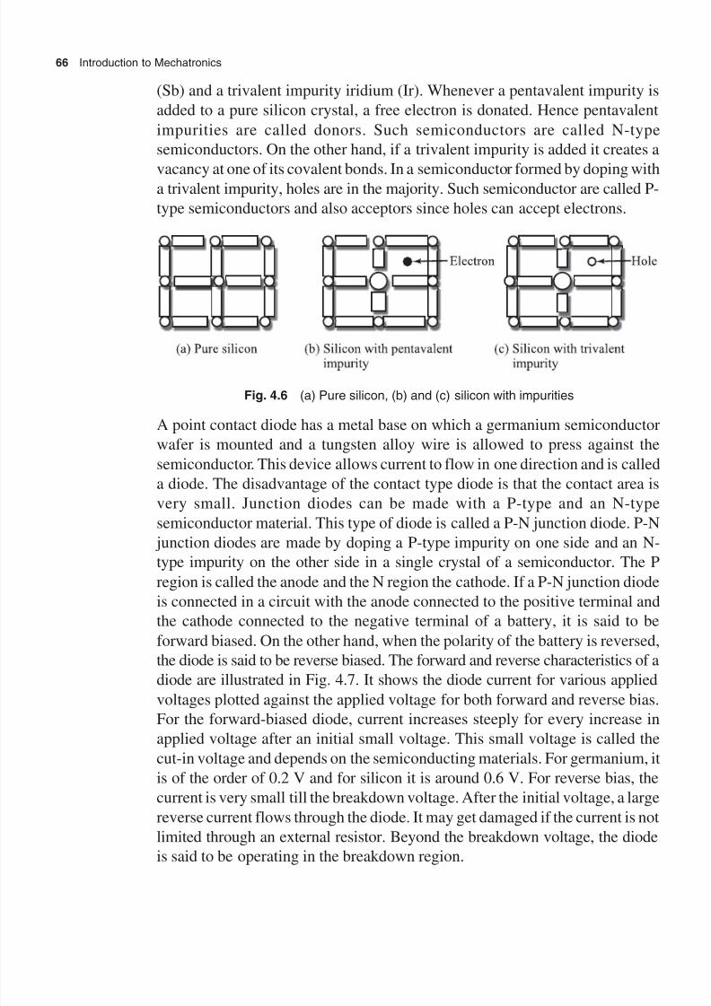
8/11/2019 Introduction to Mechatronics - Appuu Kuttan.pdf
http://slidepdf.com/reader/full/introduction-to-mechatronics-appuu-kuttanpdf 75/345
66 Introduction to Mechatronics
(Sb) and a trivalent impurity iridium (Ir). Whenever a pentavalent impurity is
added to a pure silicon crystal, a free electron is donated. Hence pentavalent
impurities are called donors. Such semiconductors are called N-type
semiconductors. On the other hand, if a trivalent impurity is added it creates a
vacancy at one of its covalent bonds. In a semiconductor formed by doping witha trivalent impurity, holes are in the majority. Such semiconductor are called P-
type semiconductors and also acceptors since holes can accept electrons.
Fig. 4.6 (a) Pure silicon, (b) and (c) silicon with impurities
A point contact diode has a metal base on which a germanium semiconductor
wafer is mounted and a tungsten alloy wire is allowed to press against the
semiconductor. This device allows current to flow in one direction and is called
a diode. The disadvantage of the contact type diode is that the contact area is
very small. Junction diodes can be made with a P-type and an N-type
semiconductor material. This type of diode is called a P-N junction diode. P-N junction diodes are made by doping a P-type impurity on one side and an N-
type impurity on the other side in a single crystal of a semiconductor. The P
region is called the anode and the N region the cathode. If a P-N junction diode
is connected in a circuit with the anode connected to the positive terminal and
the cathode connected to the negative terminal of a battery, it is said to be
forward biased. On the other hand, when the polarity of the battery is reversed,
the diode is said to be reverse biased. The forward and reverse characteristics of a
diode are illustrated in Fig. 4.7. It shows the diode current for various applied
voltages plotted against the applied voltage for both forward and reverse bias.For the forward-biased diode, current increases steeply for every increase in
applied voltage after an initial small voltage. This small voltage is called the
cut-in voltage and depends on the semiconducting materials. For germanium, it
is of the order of 0.2 V and for silicon it is around 0.6 V. For reverse bias, the
current is very small till the breakdown voltage. After the initial voltage, a large
reverse current flows through the diode. It may get damaged if the current is not
limited through an external resistor. Beyond the breakdown voltage, the diode
is said to be operating in the breakdown region.

8/11/2019 Introduction to Mechatronics - Appuu Kuttan.pdf
http://slidepdf.com/reader/full/introduction-to-mechatronics-appuu-kuttanpdf 76/345
Electronics in Mechatronics 67
The requirement of DC power supply can be met by rectifying AC supply using
a rectifier. Since the diode conducts in one direction only, it can be used as a
rectifier to convert AC into DC. If AC input is given to a diode during the
positive half-cycle, the diode is forward biased. If AC input is given to a diode
during the negative half-cycle, it is reverse biased. As the diode conducts whenit is forward biased, the positive half-cycle is transmitted to the output and it
appears across the load. To improve the average value of DC voltage, centre-
tap rectifier with two diodes or bridge rectifiers with four diode circuits are
used. The efficiency of a rectifier is measured in terms of the ripple factor.
Ripple factor is defined as the ratio of AC voltage to DC voltage. The goal of
any power supply design is to reduce this factor as much as possible. The ripple
factor is improved in the bridge rectifier configuration.
P N
(a) P-N junction diode
(c) Forward-biased
diode in circuit
(d) Reverse-biased
diode in circuit
Voltage
Current
(e) Diode characteristics
Fig. 4.7
Figure 4.8 illustrates the output waveform for a single diode with load, centre-tap
rectifier and bridge rectifier. The bridge rectifier is the most widely used rectifier.
Its main advantage is that it eliminates the requirement of a centre-tap transformer.
But the rectifier creates problems when the secondary voltage is low.

8/11/2019 Introduction to Mechatronics - Appuu Kuttan.pdf
http://slidepdf.com/reader/full/introduction-to-mechatronics-appuu-kuttanpdf 77/345
68 Introduction to Mechatronics
(a) Half-wave rectifier
(b) Centre-tap rectifier
LoadACinput
(c) Bridge rectifier
Fig. 4.8 AC to DC rectifier using diodes
Zener diode
In a normal diode the reverse breakdown occurs at a very high voltage, beyond
which the current increases steeply for every increase in applied voltage. By
varying the doping level, diodes with lower voltages from 2 to 200 V can be
manufactured. Diodes which operate in the breakdown region by reverse biasing
are called zener diodes. The voltage at which breakdown occurs is known as
zener voltage. The zener diode is of great importance for voltage regulators
since it can be used as a constant-voltage source by applying the reverse voltage
that exceeds the zener breakdown voltage.

8/11/2019 Introduction to Mechatronics - Appuu Kuttan.pdf
http://slidepdf.com/reader/full/introduction-to-mechatronics-appuu-kuttanpdf 78/345
Electronics in Mechatronics 69
Tunnel diode
By increasing the doping level one can obtain breakdown voltage at 0 V. This
will happen when the concentration of impurities is increased by more than
1000 times. The diode starts conducting at zero volt in both positive and negative
directions. Such a diode is known as tunnel diode or Esaki diode.
Light emitting diode (LED)
In a forward-biased diode, free electrons cross the junction and recombine with
holes. Whenever electrons combine with holes, energy is radiated. In a rectifier
diode this energy is liberated as heat. But in light-emitting diode, this energy is
radiated as light—red, green, yellow, orange, or infrared. LEDs producing the
visible radiation are often used in instrument displays, digital readouts, digital
clocks, calculators, etc. LEDs producing infrared radiation are used in burglar-
alarm systems.
Photodiodes
When a P-N junction of the diode is housed in a glass package, strong light
hitting the junction increases the reverse current. A photodiode is a normal
diode optimized for its sensitivity to light and is housed in a glass package. The
glass window lets the increasing light pass through the housing and hit the P-N
junction. This light produces additional holes and electrons, giving rise to higher
reverse current. Photodiodes are always used in reverse-biased conductors.
Optoisolator
An optoisolator combines an LED and photodiode in a single package. The
LED supply voltage forces a current through the LED. The light from the LED
hits the photodiode and sets up a current. If the LED current varies, the output
from the photodiode also varies. If the LED current has an AC variation, the
photodiode current will have an AC variation of the same frequency. The
resistance between the input and output is greater than 1012W.
4.3.2 Transistor
A junction transistor consists of either an N-type semiconductor sandwiched
between two P-type semiconductors or a P-type semiconductor sandwiched
between two N-type semiconductors. In the former case the transistor is referred
to as a PNP transistor and in the latter case as an NPN transistor. The
semiconductor junctions thus formed are housed in a hermetically sealed case
of either plastic or metal. Three leads are brought out from the three
semiconductor regions. The sandwiched semiconductor region is called the base.

8/11/2019 Introduction to Mechatronics - Appuu Kuttan.pdf
http://slidepdf.com/reader/full/introduction-to-mechatronics-appuu-kuttanpdf 79/345
70 Introduction to Mechatronics
The other two regions are called the emitter and the collector. The collector
region is large in size and more heavily doped. The transmitter can be considered
as two semiconductor diodes connected back to back in a crystal. Negligible
current flows through an NPN transistor with both diodes reverse biased. If
both diodes are forward biased, a large current will flow in either diode. In anNPN transistor with the emitter diode forward biased and the collector diode
reverse biased, there should be a large current in the emitter diode and negligible
current in the collector diode. But this does not happen in practice. There is a
large current in the emitter diode and an equally large current in the collector
diode also. This is referred to as transistor action. The forward-biased emitter
diode can be considered as a small resistance and the reverse biased collector
diode can be considered as a very high resistance equivalent to the back resistance
of a diode. Since collector current is almost equal to emitter current, it is clear
that in the low resistance, input is transferred to the high resistance output circuit.Figure 4.9 explains how a transistor can amplify an input signal. The emitter
diode is forward biased and collector diode is reverse biased. Hence the forward-
biased emitter can be represented as a resistance Reb having a low resistance
value equivalent to the forward resistance of a diode. Similarly, the reverse-
biased collector diode can be replaced by another resistance Rcb having very
high value. The collector current I c is about 95% of the emitter current I e and
the base current I b is about 5% of I c. The input voltage V i is the voltage across
the input resistance Reb. Here V i = I e Reb, Similarly V o = I c Rcb = 0.95 I e Rcb. The
voltage gain is given by a = V o / V i = 0.95 I e Rcb / I e Reb as I c = I e. As Rcb is very highin comparison its to Reb, the voltage gain is high. Typically Rcb is about 500 k W
and Reb is about 50 W. Voltage amplification is given by a = 0.95 ¥ 500 ¥ 103 /50
= 9500. Calculations show that the transistor can amplify an input voltage 9500
times. In this case, it is assumed that the load resistance is infinite, which is not
V =
R
R
i biased voltage
50
50 k eb
cb
=
=
W
W
I e
Reb Rcb
I c
Ib
Fig. 4.9 Transistor as amplifier
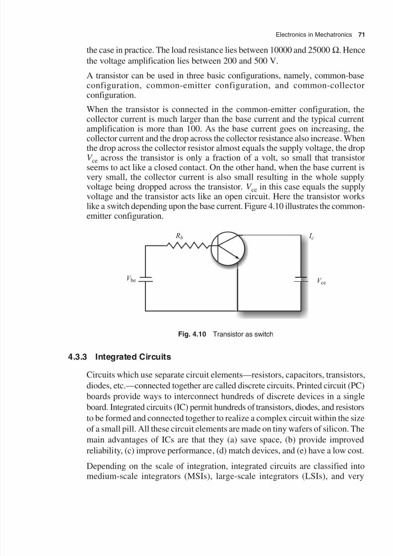
8/11/2019 Introduction to Mechatronics - Appuu Kuttan.pdf
http://slidepdf.com/reader/full/introduction-to-mechatronics-appuu-kuttanpdf 80/345

8/11/2019 Introduction to Mechatronics - Appuu Kuttan.pdf
http://slidepdf.com/reader/full/introduction-to-mechatronics-appuu-kuttanpdf 81/345
72 Introduction to Mechatronics
large-scale integrators (VLSIs). The basic structure of an IC consists of fourdistinct layers. The bottom layer is of P-type silicon, called substrate, over whichthe IC is built. The second layer is a thin N-type layer grown on the substrate.The third layer is a thin layer of silicon oxide. It acts as a barrier to protectportions of the wafer against impurity penetration. The fourth layer is an
aluminium layer which provides necessary interconnection between components.All the components are built in the second layer by a series of diffusion steps.The most complicated fabricated component is a transistor and all other elementsare constructed with one or more similar processes. Figure 4.11 shows the basicstructure of an IC (metal oxide semiconductor).
N N
P-type
Fig. 4.11 Basic structure of an IC
4.4 Digital Electronic Components
The devices used in digital systems function in a binary manner. These devices
exist in two possible states ‘on’ and ‘off’ or ‘1’ and ‘0’. A transistor used as a
digital device is used either in the cut-off or ion-saturation region and not in the
inactive region. A high voltage, 4 ± 1 V, corresponds to state ‘1’ and a low
voltage, 0.2 ± 0.2 V, corresponds to state 0.
4.4.1 Logic Gates
The building blocks of a digital system that control its output based on the
conditions of the input are called logic gates. A gate is a logic circuit with one
or more input signals but has only one output signal. The input and output
signals can consist of either high or low voltages corresponding to ‘0’ or ‘1’,
respectively. There are basically three types of gates—OR gate, AND gate, and
NOR gate. All other gates are combinations of these three.

8/11/2019 Introduction to Mechatronics - Appuu Kuttan.pdf
http://slidepdf.com/reader/full/introduction-to-mechatronics-appuu-kuttanpdf 82/345
Electronics in Mechatronics 73
The OR gate operates on both commutative and associative laws of addition.
The OR operator can be accomplished with switches in parallel. Figure 4.12
shows the symbols of the OR and NOR gates, as well as the corresponding truth
tables.
A 0
B 0 0 1 1 1 0 1 1
C 0 1 0 1 1 1 0 1
Z 0 1 1 1 1 1 1 1
0 0 0 1 1 1 1 A
B
C
Z
(a)
A 0
B 0 0 1 1 0 0 1 1
C 0 1 0 1 0 1 0 1
Z 1 0 0 0 0 0 1 1
0 0 0 1 1 1 1 A
B
C
Z
(b)
Fig. 4.12 (a) OR gate and its truth table (b) NOR gate and its truth table
The AND operation is a multiplication of two or more signals. The AND gate
can be accomplished with switches in series. The associative law holds good in
the AND gate. Figure 4.13 shows the symbols of the AND and NAND gates, aswell as the corresponding truth tables.
A 0
B 0 0 1 1 0 0 1 1
C 0 1 0 1 0 1 0 1
Z 0 0 0 0 0 0 0 1
0 0 0 1 1 1 1
A 0
B 0 0 1 1 0 0 1 1
C 0 1 0 1 0 1 0 1
Z 1 1 1 1 1 1 1 0
0 0 0 1 1 1 1
Fig. 4.13 (a) AND gate and its truth table (b) NAND gate and its truth table

8/11/2019 Introduction to Mechatronics - Appuu Kuttan.pdf
http://slidepdf.com/reader/full/introduction-to-mechatronics-appuu-kuttanpdf 83/345
74 Introduction to Mechatronics
The exclusive OR gate is known as EXOR gate and its operation is bothcommutative and associative. The symbol of an exclusive OR gate is shown in
Fig. 4.14.
A
B
C
Z
A
B
C
Z A + B + C= A + B = AB + AB = A + B + C
Bar indicates the reverse value.
Fig. 4.14 EXOR gates
4.4.2 Flip-flops
In the digital world, normally binary bits are retained or stored in a group thatrepresents either a number or a coded information. The group bits are calleddigital number system (DNS) data and are to be stored electronically. Anelectronic circuit that retains a single bit of DNS data is called flip-flop. Generally,flip-flops are used as memory devices for storing previous input values. For agiven logical level from the output, these elements are used for digital systemdevices for reset, binary conversion systems, etc. There are three types of flip-flops, namely, SR flip-flops, JK flip-flops, and D flip-flops. Flip-flops areoperated using clock cycles.
A pair of cross-connected NOR gates forms an SR flip-flop. Figure 4.15 showsthe block diagram of an SR flip-flop. It has a pair of input terminals, S and Rstanding for ‘set’ and ‘reset’, respectively. The symbols S and R not only
designate the terminals but also specify the logical level at the terminals.
S 0 0 1 1
R 0 1 0 1
Q Q 0 1
Q' Q' 1 0
×
×
S
R Q¢Q
Fig. 4.15 An SR flip-flop
Assuming Q¢ = 0, when S = R = 0, then Q = 1. The flip-flop may persist in either
of situations, one with Q = 0 and Q¢ = 1, the other with Q =1 and Q¢ = 0. The
first state refers to the reset state and the second state to the set state. The reset
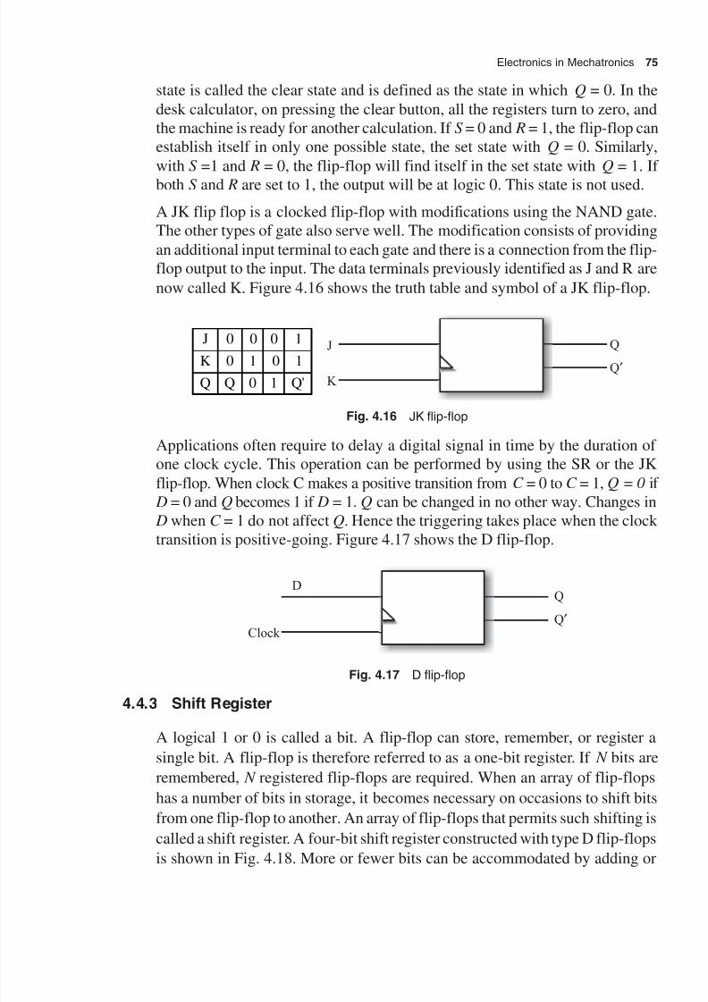
8/11/2019 Introduction to Mechatronics - Appuu Kuttan.pdf
http://slidepdf.com/reader/full/introduction-to-mechatronics-appuu-kuttanpdf 84/345
Electronics in Mechatronics 75
state is called the clear state and is defined as the state in which Q = 0. In the
desk calculator, on pressing the clear button, all the registers turn to zero, and
the machine is ready for another calculation. If S = 0 and R = 1, the flip-flop can
establish itself in only one possible state, the set state with Q = 0. Similarly,
with S =1 and R = 0, the flip-flop will find itself in the set state with Q = 1. If
both S and R are set to 1, the output will be at logic 0. This state is not used.
A JK flip flop is a clocked flip-flop with modifications using the NAND gate.
The other types of gate also serve well. The modification consists of providing
an additional input terminal to each gate and there is a connection from the flip-
flop output to the input. The data terminals previously identified as J and R are
now called K. Figure 4.16 shows the truth table and symbol of a JK flip-flop.
J 0 0 0 1
K 0 1 0 1
Q Q 0 1 Q'
J
K Q¢Q
Fig. 4.16 JK flip-flop
Applications often require to delay a digital signal in time by the duration of
one clock cycle. This operation can be performed by using the SR or the JK
flip-flop. When clock C makes a positive transition from C = 0 to C = 1, Q = 0 if
D = 0 and Q becomes 1 if D = 1. Q can be changed in no other way. Changes in
D when C = 1 do not affect Q. Hence the triggering takes place when the clocktransition is positive-going. Figure 4.17 shows the D flip-flop.
Clock Q¢
QD
Fig. 4.17 D flip-flop
4.4.3 Shift Register
A logical 1 or 0 is called a bit. A flip-flop can store, remember, or register a
single bit. A flip-flop is therefore referred to as a one-bit register. If N bits are
remembered, N registered flip-flops are required. When an array of flip-flops
has a number of bits in storage, it becomes necessary on occasions to shift bits
from one flip-flop to another. An array of flip-flops that permits such shifting is
called a shift register. A four-bit shift register constructed with type D flip-flops
is shown in Fig. 4.18. More or fewer bits can be accommodated by adding or

8/11/2019 Introduction to Mechatronics - Appuu Kuttan.pdf
http://slidepdf.com/reader/full/introduction-to-mechatronics-appuu-kuttanpdf 85/345
76 Introduction to Mechatronics
deleting flip-flops. Interconnections between flip-flops are such that the logic
level at a data input terminal is determined by the state of the preceding flip-
flop. Digital data may be presented in a serial or parallel form. In the serial
form, the data appear in a single line, one bit at a time, often synchronous with
a clock. In the parallel form, data appear at one instant of time on as many linesas there are bits. A shift register may serve as a convenient means of transforming
serial data to parallel data and vice versa.
Fig. 4.18 A four-bit shift register using D flip-flops
4.4.4 Multiplexer
Multiplexing is using an analog switching circuit which allows the connection
of a number of analog signals at a time to a common load. A multiplexer is
shown in Fig. 4.19, where four separate signals are indicated, but the number
of signals that may be involved is arbitrary. An approximate set of controllogic signals is easily generated in a four-stage ring connector. The usefulness
of the multiplex arrangement is a number of information-bearing signals (speech,
music, date, etc.) which are to be transmitted over a communication channel
through a pair of wires or a radio link to a distinct point. Multiplexing is
performed sequentially and each choice is time shared. The timing of various
input channels is controlled by a control unit. Commonly, 2 ¥ 1, 4 ¥ 2, 8 ¥ 4, and
16 ¥ 8 multiplexers are available.

8/11/2019 Introduction to Mechatronics - Appuu Kuttan.pdf
http://slidepdf.com/reader/full/introduction-to-mechatronics-appuu-kuttanpdf 86/345
Electronics in Mechatronics 77
V 1
V 2
V 3
V 4
(a) Working of a multiplexer
Telephone line
Internet connection
1 2¥
(b) Application of a multiplexer
2 1¥
Splitter Multiplexer
Ú Ú
Fig. 4.19 Multiplexer
4.4.5 Counter
A counter is an electronic device that counts. It generates a sequence of count
values determined by selected encoding and the status input. The counter can
be an up-counter or down-counter. The up-counter starts from a value to the
next larger values in the sequence and down counters do the opposite. Counters
are constructed using flip-flops. Counters can be (a) binary counters, (b) decode
counters, (c) grey counters, and (d) ring counters. Table 4.3 shows different
counter sequences for three-bit signals.

8/11/2019 Introduction to Mechatronics - Appuu Kuttan.pdf
http://slidepdf.com/reader/full/introduction-to-mechatronics-appuu-kuttanpdf 87/345
78 Introduction to Mechatronics
Table 4.3 Sequences of some counters
Binary Grey Ring Decode
000 000 001 000
001 001 010 001
010 011 100 010011 010 000 011
100 110 001 000
101 111 010 001
110 101 100 010
111 100 000 0111
Illustrative Examples
Example 4.1 A displacement resistance transducer with a shaft stroke of 100 mm is applied to a potentiometer. The total resistance of the potentiometer
is 5 W. The applied voltage is 4 V. When the wiper is at 25 mm, what is the value
of output?
Solution
The resistance at 25-mm wiper position = (25/100)5 = 1.25 k W
The output voltage = (1.25/5)5 = 1.25 V
Example 4.2 A P-N junction diode with emission coefficient 2 conducts acurrent of 240 mA through the diode with external voltage 0.8 V. Find the
value of the current through the diode at an external voltage of 0.7 V. What is
the reverse saturation current?
Solution
Current through the diode
I A = I R exp V
VT
AK
η– 1
I A = 240 ¥ 10–3A
External supply voltage, V AK = 0.8 V
Emission efficiency, h = 2
Thermal voltage, V T = 26 mV
Diode current at 0.8 V, I A1 = I Rexp
V
VT
AK 1 1η
–

8/11/2019 Introduction to Mechatronics - Appuu Kuttan.pdf
http://slidepdf.com/reader/full/introduction-to-mechatronics-appuu-kuttanpdf 88/345
Electronics in Mechatronics 79
Diode voltage at 0.7 V, I A2 = I V
VT R
AK exp 2 1
η–
Hence, I A2 = 55 mA
I R = 50 mA
Example 4.3 A logical function of four variables is f ( A, B, C , D)
= ( ) ( ) A BC B CD+ + . Express the function as a sum of products.
Solution
f ABCD A BC B CD( ) ( ) ( )= + +
= ( ) ( ) A BC B A BC CD+ + +
= AB BBC ACD BCCD+ + +
= A B BC A CD BCD+ + +
Example 4.4 Determine the value of resistance for the colour bands brown,
black, and red.
Solution
Band one, brown colour = 1
Band two, black colour = 0
Band three, red colour = 00
Hence, the resistance is 1000 W.
Example 4.5 Design a personal safe with a combination lock.
Solution
One solution could include the use of a rotary switch connected in series to
form a circuit. A three-switch diagram is shown in Fig. 4.20, which illustrates
such an arrangement. When the combination of switches is correct, a solenoid
activates the bolt of the safe to open.
Solenoid with power source
Fig. 4.20 A combination switch
Example 4.6 Design a mechatronic system for indicating water pollution in
rivers and canals.
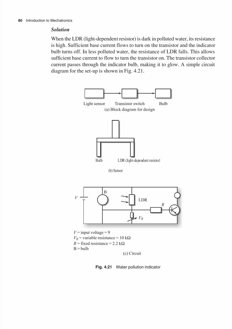
8/11/2019 Introduction to Mechatronics - Appuu Kuttan.pdf
http://slidepdf.com/reader/full/introduction-to-mechatronics-appuu-kuttanpdf 89/345
80 Introduction to Mechatronics
Solution
When the LDR (light-dependent resistor) is dark in polluted water, its resistance
is high. Sufficient base current flows to turn on the transistor and the indicator
bulb turns off. In less polluted water, the resistance of LDR falls. This allows
sufficient base current to flow to turn the transistor on. The transistor collectorcurrent passes through the indicator bulb, making it to glow. A simple circuit
diagram for the set-up is shown in Fig. 4.21.
Light sensor Transistor switch Bulb
(a) Block diagram for design
Bulb LDR (light-dependent resistor)
(b) Sensor
B
LDR R
V R
V
V
V
R
= input voltage = 9
= variable resistance = 10 k
= fixed resistance = 2.2 k
B = bulb
R
(c) Circuit
Fig. 4.21 Water pollution indicator

8/11/2019 Introduction to Mechatronics - Appuu Kuttan.pdf
http://slidepdf.com/reader/full/introduction-to-mechatronics-appuu-kuttanpdf 90/345
Electronics in Mechatronics 81
Exercises
4.1 Differentiate between an insulator, a conductor, and a semiconductor.
4.2 Write notes on passive devices used in electronic circuits.
4.3 Distinguish between the zener diode, tunnel diode, LED, and photodiodes.
4.4 Explain the use of transistors as amplifiers.
4.5 Explain the use of transistor as a switching device.
4.6 Explain the working of OR, NOR, AND, NAND, and EXOR gates.
4.7 A logical function of five variables is f ( A, B, C , D, E ) = A BC D BE + + .
Express the function as a sum of products.
4.8 What is the use of a flip-flop? Explain the working of a shift register usingflip-flops.

8/11/2019 Introduction to Mechatronics - Appuu Kuttan.pdf
http://slidepdf.com/reader/full/introduction-to-mechatronics-appuu-kuttanpdf 91/345
Computing Elements in Mechatronics
Mathematical instruments are used to generate or to solve mathematical functionssuch as trigonometric functions, hyperbolic functions, exponential functions,quadratic equations, equations of high order, differential equations, integration,etc. In these instruments, signals are continuous, analog, and without time delay.
The calculating mechanism involved is similar to the one involved in calculatingand adding machines, where all the operations are performed with adiscontinuous or a digital signal. The computer is a device that involves thegeneration and solution of mathematical functions, and involves calculatingmechanisms. The computer that operates for the mathematical function andcan accept any analog signal is called the analog computer. The computer that
can make calculations or digital computations is called the digital computer.The first calculating machine was developed by Pascal in 1642 in order to helphis father, who collected taxes in France.
The first step-up drums principle with digital transfer was developed by themathematician and philosopher Lecibniz in 1672, but he did not develop amachine. Ohhner in 1878 in Sweden fabricated a calculating machine and
industries started using such machines. Figure 5.1 illustrates the differencebetween an analog signal and a digital signal.
Fig. 5.1 Analog and digital signals

8/11/2019 Introduction to Mechatronics - Appuu Kuttan.pdf
http://slidepdf.com/reader/full/introduction-to-mechatronics-appuu-kuttanpdf 92/345
Computing Elements in Mechatronics 83
In the last 50 years, semiconductor technology has undergone many changes.Integrated circuits (ICs) appeared on the scene at the end of the 1950s, followedby the invention of the transistor. In the early 1960s, logic gates belonging towhat is known as the 7400 series were commonly available as ICs and thetechnology of integrating the circuits of a logic gate on a single chip became
known as small-scale integration (SSI). As semiconductor technology advanced,more than hundred gates were fabricated on one chip, which was called medium-scale integration (MSI). A typical example of MSI is the decoding counter 7490.At the end of the twentieth century, it was possible to fabricate more than 1000gates on a single chip, which was known as large-scale integration (LSI). Thatwas an era of very large-scale integration (VLSI) and super large-scale integration(SLSI). The lines of demarcation between these different scales of integrationare ill-defined and arbitrary. With the advancement of computer technology,the digital computer as well as the analog computer used semiconductor devices.Digital computers are more popular than analog computers, since analog signalsolutions can also be easily obtained by calculation through the difference
differential equation of a function.
5.1 Analog Computer
The heart of an analog computer is the operational amplifier. Operationalamplifiers (op-amps) are commercially available in the form of ICs. Theseamplifiers are generally intended to operate linearly rather than in a digitalswitching mode. However, op-amps do serve as components in sample andhold circuits in multiplexers and in circuits used for analog to digital conversion
and vice versa.
e1
e2
Aeo e1
Z s I 2
e0
I 1
Z f
(a) Symbol of op-amp (b) Basic circuit of an op-amp
Fig. 5.2 The operational amplifier
As shown in Fig. 5.2 (a), an op-amp has two inputs, e1 and e2, to accommodatetwo input signals and a single output signal eo. The output voltage of anop-amp is equal to the difference between the two input voltages multiplied bya high voltage gain. The voltage gain at low frequency is a large real positivenumber, and can be as large as 5 ¥ 104.
Referring to Fig. 5.2(b), Z s is the series impedance and Z f is the feedback
impedance. Using Kirchhoff’s law,

8/11/2019 Introduction to Mechatronics - Appuu Kuttan.pdf
http://slidepdf.com/reader/full/introduction-to-mechatronics-appuu-kuttanpdf 93/345
84 Introduction to Mechatronics
Current I e e
Z s1
1 2=–
and I e e
Z
o g
f
2 =–
Since an op-amp is a high-gain element, there is virtually no current flow. Hence
I 1 = I 2. Equating the current and rearranging, we get
eo
Z
Z e
Z
Z e
Z
Z e
f
s
i
f
s
g
f
s
g= + +
Since eg = eo / A and A has very large value,
e Z
Z eo
f
s
i= –
This is the basic principle of an op-amp. With appropriate selection of feedback
impedance and series impedance, it can be used as a multiplier, adder, integrator,
or differentiator. Figure 5.3 illustrates the applications of the op-amp for various
operations.
R
ei
R f
eo
R1
R2
R3
R f
eo = – ( / ) R R e f i
Re
= resistance= input/output voltage
eo = –[( / ) + ( / ) + ( / ) )]if = = = , = [ ( + + ]
R R e R R e R R e R R R R e e e e
f f f
f o
1 2 3
1 2 3 1 2 3 –
(a) Multiplier (b) Adder
eo
R
ei
C
E 0
eiC
R
eo
e = – o1
RC e dt + E i 0 e = – o
1 Re
dei
dt
E – The constant of integration, initial charge of the capacitor.0
(c) Integrator (d) Differentiator
Fig. 5.3 Applications of the op-amp

8/11/2019 Introduction to Mechatronics - Appuu Kuttan.pdf
http://slidepdf.com/reader/full/introduction-to-mechatronics-appuu-kuttanpdf 94/345

8/11/2019 Introduction to Mechatronics - Appuu Kuttan.pdf
http://slidepdf.com/reader/full/introduction-to-mechatronics-appuu-kuttanpdf 95/345
86 Introduction to Mechatronics
1
Fl p-flopi Transistor
3
71
5
6
8
4
(b) Equivalent circuit
2
8
Fig. 5.5 LM 555 timer
Pin 8 is connected to the supply voltage, which ranges from + 5 V to 8 V. Pin 1is the ground terminal l and pin 2 is called the trigger terminal. It is an ONswitch for the output pulse. The output is taken from pin 3. Figure 5.5 illustrates
the pin configuration and equivalent circuit of an LM 555 timer.
5.3 Analog to Digital Conversion
Analog to digital converters (ADCs) are required to convert analog signals fromsensors into a digital form, compatible with a personal computer's digital input.Generally, analog to digital converters are complex and sophisticated systems.There are many possible schemes for A/D conversion and many variations arepossible within each scheme. Comparators with register ADCs in chip formsare commonly used. Figure 5.6 illustrates the pin configuration and equivalent
circuit of the 8-bit ADC. ADCs are available for 8-, 10-, 16-, 22- and 24-bitdigital conversion. The internal details of analog to digital conversion are asfollows. There is a component with the analog output V o, outputs as the digitalparallel bits b1 to b8, the voltage reference V r , the collector–ground voltage V s,the analog ground, and the digital ground.
The analog input V i is compared to the ADC output V o and if V o < V i, the output
of the comparator becomes high. If V o > V i, the output of the comparator is low.The digital content of the register b1 to b8 starts at 00000000 and is modified ineach clock cycle to induce a trial-and-error process. At the end of this process,the digital output of the register b1 to b8 is sent to the pins 13 to 20 as the paralleldigital output of the ADC. The clock frequency is often from 0.25 to 80 MHz
such that the clock cycle time, the inverse of the clock frequency, is 0.0125 ms.
The conversion of an analog signal into an n-bit digital number leads to arepresentative that has 2
n distinct digital values. The quantization error or resolution
corresponds to the smallest change in the digital conversion. In the case of input

8/11/2019 Introduction to Mechatronics - Appuu Kuttan.pdf
http://slidepdf.com/reader/full/introduction-to-mechatronics-appuu-kuttanpdf 96/345
Computing Elements in Mechatronics 87
voltagesV i larger than V N , the conversion is saturated by V N and these input voltagesare represented by the largest digital n-bit number. This error due to saturationcan be reduced by signal conditioning to match the range of input voltages with
one of the selectable scales such that the maximum V i < V N .
1
11 12
22
3. start4. status5. input signalV s
6. digital signal7. analog outputV i
8. analog ground11. reference inputV R
12. to 20 to , digital outputb b1 8
b b1 —LSB and MSB8 —
(a) Pin assignment for 8-bit ADC
2
34
5
6
7
8
910
21
19
18
17
16
15
14
13
20
1
2
3
4
5
6
78
9
10
11
22
Control logic Cock
V N
64 R
1 R
(b) Equivalent circuit
21
2019
18
17
16
15
14
13
12
Fig. 5.6 The 8-bit ADC
In the case of input voltages V i with maximum V i < V N , the part of the scale between
maximum V i and V N is not used and the resolution of the digital conversion isreduced. Consequently the analog input voltage V i has to be normalized on a0 –V N scale, where V N is the upper limit of the scale. The ideal selection is maximum
V i ª V N . Often, ADC boards have selectable scales with V N of 0.1, 1, or 10 V. V N is
determined by the full-scale range voltage given by V fsr = 2 R f V R / R, where R f is the
feedback resistance of the summing op-amps. Given that the resolution r for a nominal
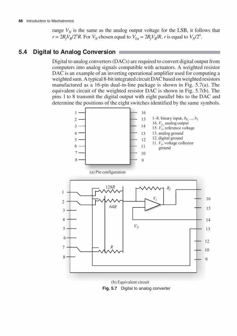
8/11/2019 Introduction to Mechatronics - Appuu Kuttan.pdf
http://slidepdf.com/reader/full/introduction-to-mechatronics-appuu-kuttanpdf 97/345
8/11/2019 Introduction to Mechatronics - Appuu Kuttan.pdf
http://slidepdf.com/reader/full/introduction-to-mechatronics-appuu-kuttanpdf 98/345
Computing Elements in Mechatronics 89
For the value bi (i = 1 – 8), the corresponding switch is connected by a thick line
to the common digital ground, pin 12. There is a resistance 2i–1 R. For example,
between the reference voltage V R and the input voltage V N , for the op-amp, for
b1=1, the resistance is 20 R = R, while for b2 = 0, the resistance is infinity. For
b7 = 1, the resistance is 26 R and changes to 64 R. The relationship between theinput V R and the output V o of the inverting amplifier is obtained as
V R
RV o
f
R= –
where in this case R f is the equivalent resistance resulting from all parallel
resistances associated with switches in the position corresponding to bi = 1
(i = 1 – 8), such that
1
2 1281
1 2 8
R
b
R
b
R
b
R
= + +º+
( )7 6 01 2 8
1
1 12 2 2
128b b b
R R
…= + + +
The foregoing input–output relationship becomes
V RV
R
b b bo
R=
+ +º+
–
2
2 2 2
1 2
2
8
8
A binary number b1, b2, ..., b8 has the decimal equivalent (27b1 + 2
6b1 +
...+ 20b8).
The bit b1 is the most significant bit (MSB) and the bit b8 is the least significantbit (LSB). The resolution has the same value as the V o LSB, given the LSB that
corresponding to the smallest change in output voltage V o. For an n-bit DAC,
V R V
Rb b b
Ro
R n nn n
= +
+ +º+
-– –2 2 2 2
1
2
11
22
0
=
+ +…+
– 2
2 2 2
1 2
2 R
V
R
b b b R n
n
The full-scale range voltage is defined as
V fsr = 2 R f V R / R
5.5 Digital Computer
The abacus is a primitive calculator made up of beads. It was first made in 5000
BC in China. It was the first calculating machine. In about 500 BC, the Greeks
began to use the abacus. From the fifteenth century to the beginning of the
twentieth century, various calculating machines which used mechanical elements

8/11/2019 Introduction to Mechatronics - Appuu Kuttan.pdf
http://slidepdf.com/reader/full/introduction-to-mechatronics-appuu-kuttanpdf 99/345
90 Introduction to Mechatronics
were developed. The first solid state computer was made in 1960. In 1960,
computers were accessible and affordable only to large corporations, big
universities, and government agencies. Because of advancement in
semiconductor technology, the million dollar computing capacity of the 1960s
is now available for less than ten dollars in an integrated circuit called themicroprocessor. A computer working on a microprocessor is called a
microcomputer. Microcomputers are nowadays making an impact on every
aspect of our lives and in industrialized societies. The basic structure of a
microcomputer is not different from any other computer. The computers
communicate and operate using digital signals. Each computer can accept a set
of instructions in the form of a binary pattern called a machine language. Since
it is difficult for people to communicate with the computer in the language of
0’s and 1’s, binary instructions are given abbreviated names, called mnemonics,
which form the assembly language for a given computer.A digital computer is a multipurpose, programmable machine that reads binary
instruction from its memory, accepts binary data as input, processes data
according to those instructions, and provides results as output. The physical
components of a computer are called hardware. A set of instructions written for
the computer to perform a task is called a program, and a group of programs is
called software.
The Motorola 6800 microprocessor has a set of binary codes and mnemonics
entirely different from those of 8085/8080A. An assembly language program
written for a microprocessor is not transferable to a computer with another
microprocessor unless the two microprocessors are compatible in their machine
codes. Machine language and assembly language are considered as low-level
languages. In the case of assembly language, mnemonics get translated into a
binary code using an assembler. The programming languages that are intended
to be machine-independent are called high-level languages. These include such
languages as FORTRAN, BASIC, PASCAL, and COBOL. The English words
are translated into binary language through another program called the compiler
or interpreter. The compiler or interpreter requires a large memory space.
Different types of computers are designed to serve different purposes. The
microcomputer is defined as a computer with microprocessors as the central
processing unit. Large computers have various types of microprocessors
performing different functions within a large CPU. In 1994, the fifth generation
computer was established. Such a computer was called a supercomputer. It is
smart, fast, and performs large computations. Typically a supercomputer
accomplishes 64,000 processes per second. A microcomputer system consists
primarily of four components, the microprocessor, memory, input, and output.

8/11/2019 Introduction to Mechatronics - Appuu Kuttan.pdf
http://slidepdf.com/reader/full/introduction-to-mechatronics-appuu-kuttanpdf 100/345
Computing Elements in Mechatronics 91
5.6 Architecture of A Microprocessor
The microprocessor manipulates data, controls the timing of various operations,
and communicates with input/output devices and memory. The internal logic
design of a microprocessor is called its architecture. The microprocessor consists
of three basic units. The basic units are the central processing unit (CPU) torecognize and carry out program instructions, the input and output circuit
interface, and the memory to retain the program instructions and data. The input/
output arrangement is used to send out or feed data. The data bus is used to
transfer a word to and from the CPU. The address bus bar carries signals which
indicate what data is to be found and selected. The control bus is the means by
which signals are sent to synchronize the separate elements. In microprocessors,
the memory and various input and output arrangements are all arranged in one
chip called the microcontroller. Different types of microprocessors are available.
Commonly, a single-chip microprocessor is used. The different types ofmicroprocessors are 8085, 8086, z80, and 68000. Figure 5.8 shows the basic
structure of a microprocessor and pin configuration and internal structure of
the 8085 chip.
The internal architecture of the 8085 microprocessor determines how an
operation can be performed with the given data and also which operations can
be performed. These operations are (a) storing 8-bit data, (b) performing
arithmetic and logical operations, (c) testing for conditions, (d) sequencing the
execution of instructions, and (e) storing data temporarily during execution in
the defined read/write memory location.
To perform these operations, the microprocessor requires registers, an arithmetic
logic unit, a control logic unit, and internal buses. The 8085 is an 8-bit general-
purpose microprocessor capable of addressing 64K of memory. The device has
40 pins, requires a +5 V single power supply, and can operate with a 3-MHz
single phase clock.
In the signal line b0 to b7, all the bi’s are bidirectional. They are used for a dual
purpose, as the low-order address bus as well as the data bus. This is also known
as multiplexing the bus. The control groups of signals include two central signalsRD and WR, and three status signals IO/M, S1, and S0, which identify the nature
of the operation. One special signal, ALE, indicates the beginning of the
operation. RD reads the control signal. This signal indicates the selected input/
output or memory devices to read and data availability in the address bus bar.
WR writes data on the data bus in a selected memory or input/output (I/O)
location. IO/M is a status signal used to differentiate between I/O and memory
operations. When it is high, it indicates input/output operation and when it is
low, it indicates memory operation. S1 and S2 are status signals, similar to IO/

8/11/2019 Introduction to Mechatronics - Appuu Kuttan.pdf
http://slidepdf.com/reader/full/introduction-to-mechatronics-appuu-kuttanpdf 101/345
92 Introduction to Mechatronics
M, which can identify various operations; but they are rarely used in small
systems.
Memory CPU Input/
output
Address bus bar
Data bus
Control bus bar
(a) Structure of a microprocessor
1 40
(b) Pin configuration of 8085
1. X12. X23. SOS4. STD
5. STD6. TRAP7. RESET8. RST 659. INTR
10. INTR 12 – 20. binary input21 – 28. additional
binary input
29. SO30. ACR 31. WR
32. RD33. SF34. 1.035. READ36. RESET37. C/R out38. HLDA39. HOLD40. Vcc
2
34
5
6
7
8
9
10
11
12
13
1415
16
17
18
19
20
39
3837
36
35
34
33
32
31
30
29
28
2726
25
24
23
22
21

8/11/2019 Introduction to Mechatronics - Appuu Kuttan.pdf
http://slidepdf.com/reader/full/introduction-to-mechatronics-appuu-kuttanpdf 102/345
Computing Elements in Mechatronics 93
Fig. 5.8 The 8085 microprocessor
V cc is + 5 V and V ss is the ground. X1 and X2 are crystals connected to the pin.
The frequency is internally divided into two. To operate at 3 MHz, the crystal
should have 6 MHz. CLK(out) can be used as the system clock for other devices.
The 8085 microprocessor has five interrupt signals that can interrupt a programexecution. INTRA is an interrupt request. It acknowledges the interrupt signal.
In addition to the interrupt, three pins—RESET, HOLD, and READY—accept
externally initiated signals. INTRA responds to HOLD request. INTRA
acknowledges the same kind of signal from HLDA. When the RESET in the
signal becomes low, the program counter is set to zero. RESET OUT indicates
that the MPU is reset. The signal can be used to reset other devices. For serial
transmission, SID (serial input data) and SOD (serial output data) are used.

8/11/2019 Introduction to Mechatronics - Appuu Kuttan.pdf
http://slidepdf.com/reader/full/introduction-to-mechatronics-appuu-kuttanpdf 103/345
94 Introduction to Mechatronics
5.7 Microcontroller
For a microprocessor to give a system that can be used for control, additional
chips are necessary. For instance, memory devices for program and data storage
and input/output ports allow it to communicate with the external world and
receive signals from it. The microcontroller is the integration of a microprocessor
with memory and input/output interfaces and other peripherals such as a timer
on a single chip. Figure 5.9 shows the general block diagram of a microcontroller.
The general microcontroller has pins for external connection of inputs and
outputs, power, clock, and control signals. The pins for the input and output are
grouped into units called input/output ports. Usually, such ports have eight lines
in order to be able to transfer an 8-bit word of data. Two ports may be used for
a 16-bit word, one to transmit the lower 8-bit portion and the other to transmit
the upper 8-bit portion. The port can be input only, output only, or programmableto be either input or output.
The Motorola 68HC II, the Intel 8051, and PIC 16C6x17x are examples of 8-bit
microcontrollers, which have the data path of 8 bits. The Motorola 68HC16 is a
16-bit microcontroller and Motorola 8300 is a 32-bit microcontroller. These
have a limited amount of ROM (read only memory) and RAM (random access
memory) and are widely used for embedded control systems.
I/O
ports
Memory
CPU
Register
Clock
Controllines
Fig. 5.9 Block diagram of a microcontroller
8/11/2019 Introduction to Mechatronics - Appuu Kuttan.pdf
http://slidepdf.com/reader/full/introduction-to-mechatronics-appuu-kuttanpdf 104/345
Computing Elements in Mechatronics 95
A microprocessor system with separate memory and input/output chips is more
suited for processing information in a computer system. While selecting a
microcontroller, the following factors are considered.
1. Number of input/output pins
2. Interfaces required
3. Memory requirement
4. Number of interrupts required
5. Processing speed required
Microcontrollers are used in temperature-measuring systems, domestic washing
machines, and many industrial applications.
5.8 Programmable Logic Controller
A programmable logic controller (PLC) is a digital electronic device that uses a
programmable memory to store instructions and to implement functions such
as logic, sequence, timing, counting, and arithmetic in order to control machines
and processes. Such controllers have been specifically designed to make
programming easy. The term ‘logic’ is used because the programming is
primarily concerned with the implementation of logic and switch operations.
Input devices such as switches and output devices such as motors being controlled
are connected to the PLC and then the controller monitors the input and output
according to the program stored in the PLC by the operator and so controls the
machine or process. The PLC has the great advantage that it is possible to modify
a control system without having to remove the connections to the input and
output devices, the only requirement being that an operator has to key in a
different set of instructions. PLC-operated systems are much faster than relay-
operated systems. A PLC is smaller than a computer, but has certain features
given below that are specific to their use as controllers.
1. They are rigid and designed to withstand vibration, temperature, humidity,
and noise.2. The interfacing circuit for input and output is inside the controller.
3. They are easily programmed and have an easy programming language.
Programming is primarily concerned with logic and switching operations.
PLCs were first conceived in 1968. They are now widely used and extend from
small self-contained units for use with perhaps 20 digital input/output to modular
systems that can be used for a large number of input/output units. They also
handle digital and analog input/output.

8/11/2019 Introduction to Mechatronics - Appuu Kuttan.pdf
http://slidepdf.com/reader/full/introduction-to-mechatronics-appuu-kuttanpdf 105/345
96 Introduction to Mechatronics
The input/output channel provides signal conditioning and isolation functions
so that sensors and actuators can generally be directly connected without need
for other circuitry. The common output voltages are 24 V and 240 V. The outputs
are specified as relay type, transistor type, and triac type. In the relay- type
output, the signal from the PLC output is used to operate a relay and so is ableto switch currents of the order of few amperes in an external circuit. The relay
isolates the PLC from the external circuit and can be used for both AC and DC
switching. The relays are relatively slow to operate. The transistor-type output
uses a transistor to switch current through the external circuit. This gives a
faster switching action. Optical isolators are used with transistor switches to
provide isolation between the external circuit and the PLC. The transistor output
is only for DC switching. A triac can be used to control external circuits, which
are connected to the AC power supply.
Fig. 5.10
PLC programming based on the use of the ladder diagram involves writing a
program in a manner similar to drawing a switching circuit. The ladder diagram
consists of two partial lines representing the power rails. The circuits are

8/11/2019 Introduction to Mechatronics - Appuu Kuttan.pdf
http://slidepdf.com/reader/full/introduction-to-mechatronics-appuu-kuttanpdf 106/345
Computing Elements in Mechatronics 97
connected as horizontal lines. The rugs of the ladder are between the vertical
lines. Figure 5.10 shows the basic standard ladder symbols as well as examples
of rugs in a ladder diagram. In drawing the circuit line for rugs, inputs must
always precede outputs and there must be at least one output on each line. Each
rug must start with an input or a series of inputs and end with outputs. Theinputs and outputs are members of the ladder diagram. The notations are used
depending on the PLC manufacturer. The Mitsubishi F series of PLCs precedes
the input element by an X and the output element by a Y as shown in the following
example:
Inputs X400-407, 410-413
X500-507, 510-513 (24 possible inputs)
Outputs Y430-437
Y530-537 (16 possible inputs)
5.9 Computer Peripherals
The purpose of the input/output section of a computer is to provide communication
with the variety of peripheral devices used with the computer system. Input/output
devices have two inverse functions. First, it must interpret the incoming signals
and hold them temporarily until they are placed in the main memory of the CPU.
Second, the result of the calculation and data processing operation must be
transmitted to the appropriate peripheral equipment.
5.9.1 Hardware Devices Used for Computer Storage
The programs and data files are not generally kept in primary storage, but are
stored on large-capacity auxiliary devices and loaded in to the main memory as
required. The auxiliary devices constitute the secondary storage and are
physically external to the computer, which means that the programs and data
files are not directly available to the CPU. There are two basic types of secondary
storage: (a) sequential access storage and (b) direct access storage.
The sequential storage method has a substantially lower access rate than the
direct access storage method. The magnetic tape storage is a prime example of
the sequential access storage technology. Data is stored on magnetically coated
Mylar tape, similar to the magnetic tape used in audio systems. The recording
and reading data are nondestructive, which means that the tape can be erased
and reused. Since data are stored sequentially, the access time is relatively slow.
However, the low cost per bit and the high capacity of magnetic tapes make it
ideal for system backup.

8/11/2019 Introduction to Mechatronics - Appuu Kuttan.pdf
http://slidepdf.com/reader/full/introduction-to-mechatronics-appuu-kuttanpdf 107/345
98 Introduction to Mechatronics
The magnetic drum is a random access storage device with high capacity and
high access rates. It consists of a magnetically coated cylinder. During operation,
the drum rotates at a constant speed and data are recorded in the form of
magnetized spots. The drum can be read repeatedly without causing data loss.
Read/write heads are used to read data to and from the drum as it rotates. Thedrum surface is divided into tracks, each with its own read/write head.
The magnetic disk storage is also a direct access storage device. The storage
medium is a magnetic disk. There are several types and sizes of disks, each best
suited to a particular set of applications. The flexible floppy diskette comes in
several standards—3½ inch, 5½ inch, 8 inch, etc.—and is packaged in a square
plastic envelope to protect the magnetic surfaces. Reading and writing are
accomplished through access holes in the envelope. Floppy disks are available
with either one or both sides used for storing data. The hard disk is a thin metaldisk which is coated on both sides with magnetic ferric disks. The data are
recorded in the form of magnetized spots on tracks on the disk surface. Several
disks are combined into a single disk pack and these are separated by a fixed
distance and joined by a vertical shaft. The disk pack is rotated at several thousand
revolutions per minute by a disk drive unit. The data are transferred by many
sets of read/write heads (one per recording surface) to the appropriate track.
The rate of operation is usually several thousand bytes per second.
Bubble memory consists of microscopic magnetic bubbles on a thin crystalline
magnetic film. It has high storage density and random address capabilities.
However, because of its high cost, the technology is not yet competitive with
other memory technologies.
Optical data storage using laser beams is widely used in the form of compact
disks (CDs). The data are stored as microscopic bits on a metallic surface. The
data are read by directing a laser beam across the surface and measuring the
wavelength of light reflected. This reflected light can be converted into electrical
pulses. The storage medium is metal film strips, arranged into tracks.
R/WM (read/write memory)
Read/write memory is popularly known as random access memory (RAM).
This memory is volatile, meaning that when power is turned off, all the contents
are destroyed. Two types of R/W memories are available–static and dynamic.
Static memory is made up of flip-flops and stores a bit as voltage. Dynamic
memory is made of metal oxide silicon (MOS) transistor gates and stores a bit
as a charge.
8/11/2019 Introduction to Mechatronics - Appuu Kuttan.pdf
http://slidepdf.com/reader/full/introduction-to-mechatronics-appuu-kuttanpdf 108/345
Computing Elements in Mechatronics 99
ROM (read only memory)
The ROM is nonvolatile, meaning that it retains the stored information even if
the power is turned off. ROM uses diodes arranged in a matrix format. Four
types of ROM are presently available, MASKED ROM, PROM, EPROM, and
EEPROM.
Masked ROM
In this ROM, a bit pattern is permanently recorded by the masking and
metallization process, which is an expensive and specialized process. The
manufacturer produces quantities in thousands, considering the economy.
PROM (programmable read only memory)
This memory has nichrome or polysilicon wires arranged in a machine. The
wires can be functionally varied as diode or fuse. This memory can beprogrammed by the user with a special PROM program that selectively burns
the fuse according to the bit pattern required to be stored.
EPROM (erasable programmable read only memory)
The information stored in this memory is semi-permanent. All the information
can be erased by exposing the memory to ultraviolet light through a quartz
window installed on the chip. The memory chip can be reprogrammed again
and again.
EEPROM (electrically erasable PROM)
This memory is functionally similar to EPROM, except that the information
can be altered by using electrical signals at the register level rather than erasing
all the information. At present, it is expensive and not commonly used. The
interface of 1024(1K) bytes read/write memory to an 8085 system, with the
many maps from 3000H to 33FFH, uses 2114(1024 ¥ 4) memory chips and the
74LS318, 32.3 to 8 decoder. The memory chip 2114 is a static memory organized
in 1024 ¥ 4 formats, which means that it has 1024 registers with four input–
output lines. Two chips must be connected in parallel to form an 8-bit memory.
5.9.2 Computer Input Devices
The operator input devices are provided with the computer to facilitate
convenient communication between the user and the system. Punched cards
have been used more during its long existence than any other data recording
medium. There are two types of punched cards—the 80-column Hollerith card
and the 96 column IBM card.
8/11/2019 Introduction to Mechatronics - Appuu Kuttan.pdf
http://slidepdf.com/reader/full/introduction-to-mechatronics-appuu-kuttanpdf 109/345
100 Introduction to Mechatronics
There are two types of card readers currently in use—the brush reader and the
photoelastic reader. In the first case, the punched cards are moved past a cell of
conductive brushes. In the latter case, the devices use a cell of photocells and a
light source which shines through the hole in the card to produce electrical
pulses. The magnetic tape units were introduced because of the demand for fast
input/output devices. They can be used for program and data storage and can be
interfaced to the computer as both input and output units.
Basically, input devices are classified as (a) cursor control devices, (b)
digitalizers, and (c) alphanumeric and other key-based terminals.
The cursor normally takes the form of a bright spot or an arrow on the cathode
ray tube screen. The computer is capable of reading the current position of the
cursor. A variety of cursor control devices have been employed in computer
systems. These include thumbwheels, direction keys on a keyboard terminal,
the joystick, trackball, cursor, light pen, and electronic tablets. The first five
items in the list provide control over the cursor without direct physical contact
on the screen by the user. The last two devices in the list require the user to
control the cursor by touching on the screen.
The thumbwheel devices use two thumbwheels, one to control the horizontal
position of the cursor, and the other to control the vertical position. The cursor
in this arrangement is often represented by the intersection of a vertical and a
horizontal line displayed on the screen. The cursor can also be controlled by
using the direction keys on the key branch. Four keys are used for each of thefour directions in which the cursor can be moved—right or left and up or down.
The joystick apparatus consists of a box with vertical toggle state that can be
pushed in any direction to cause the cursor to be moved in that direction. The
joystick gets its name from the control stick that was used in aeroplanes. The
track ball and mouse operation is similar to that of the joystick except that, in
this case, an operator ball is rotated to move the cursor in the desired direction
on the screen. In the mouse, the body is moved to allow for rotation of the ball
due to surface friction, which in turn allows the cursor to move.
The light pen is a pointing device in which the computer seeks to identify the
position where the light pen is in contact with the screen. The light pen is a
detector of the light on the screen and uses a photodiode, phototransistor, or
some other form of light sensor. The tablet and pen in a computer describe
electronically sensitive tablets which work in conjunction with an electronic
stylus. The light pen and tablet/pen are used for other inputs such as selecting a
function from the menu and selecting an operation on the screen for enlargement
as well as cursor control.

8/11/2019 Introduction to Mechatronics - Appuu Kuttan.pdf
http://slidepdf.com/reader/full/introduction-to-mechatronics-appuu-kuttanpdf 110/345
Computing Elements in Mechatronics 101
The digitizer is an operator input device consisting of a large, smooth band andan electronic tracking device which can be moved over the surface to follow theexisting lines. It is a common technique for tracking X and Y coordinates from
a paper drawing. Such devices contain a switch for the user to record the desired X and Y coordinate positions. The digitizer can be used to digitize line drawings.
The user can input data from a rough schematic or long drawing and edit thedrawing to the desired level of accuracy. For computer aided drawing, a three-dimensional digitizer can be made use of to draw a wire frame model three-dimensional objects.
Several forms of keyboard terminals are available as input devices for thecomputer. The most familiar type is the alphanumeric terminal. Such terminalsare used to enter commands, functions, and supplemental data to the computer.Some computers make use of special function keyboards to eliminate extensivetyping commands. The number of function keys varies from 8 to 80. The
transmission speeds are usually selectable from 110 to 960 band. A band is aunit representing the number of discrete signal changes per second. For a binarysystem, it is equal to number of bits per second.
5.9.3 Computer Output Devices
All the computer terminals available today use the cathode ray tube (CRT) asthe display. The operation of the CRT is illustrated in Fig. 5.11. A cathode emitsa high-speed electron beam onto a phosphor-coated glass screen. The electrons
(a) Cathode ray tube
(b) Stroke writing (c) Raster scan
Focusingsystem
CathodeDeflectionsystem
Electron beam
Phosphor-coatedscreen
Fig. 5.11 Cathode ray tube terminals

8/11/2019 Introduction to Mechatronics - Appuu Kuttan.pdf
http://slidepdf.com/reader/full/introduction-to-mechatronics-appuu-kuttanpdf 111/345
102 Introduction to Mechatronics
energize the phosphor coating, causing it to glow at the points where the beam
makes contact. By focusing the electron beam, changing its intensity, and
controlling its point of contact against the phosphor coating through the use of
a deflection system, the beam can be made to generate a picture on the CRT
screen. There are two basic techniques used in current computer terminals and
CRT screens. They are (a) stroke writing and (b) raster scan.
The stroke writing technique includes line drawing, random positioning, vector
writing, stroke writing, and directed beam. The stroke writing system uses an
electron beam, which operates like a pencil to create a line image on the CRT
screen. The image is constructed out of a sequence of straight line segments.
There are various types of output devices used for permanent record in
conjunction with the cathode ray tube terminal. The line printer is the most
commonly used terminal device used in computers. There are three types of
line printers—the drum printer, the chain printer, and the optical printer.
The basic component of a drum printer is the drum with the complete character
set embossed on its periphery. Opposite to each character position on the drum,
there is a print hammer. The hammer is fixed and the required character is
aligned with the hammer as the required output. The speed of the modern drum
printer is in the range of 600 to 1300 lines/min. There are various types of print
hammer mechanisms, and those with the least number of moving parts are the
most reliable. Normally, a voltage is sent to operate a solenoid associated with
the hammer selected for the printer. When the correct character on the
continuously rotating drum is in the printing position, the pulses which operatethe hammer mechanism may give direct drive to the solenoid armature, so that
the hammer, which is part of the armature, impresses the paper up to a preset
stop. This is what happens in a penetration-type printer. The pulse to the solenoid
may cause the solenoid armature to strike a separate piece of metal which projects
on the paper and return by spring action. This is what happens in a ballistic
printer. Figure 5.12 shows the hammer mechanism with a printing hammer.
Paper
DrumRibbon
Hammer Spring
Electromagnet
Fig. 5.12 Hammer mechanism for a drum printer

8/11/2019 Introduction to Mechatronics - Appuu Kuttan.pdf
http://slidepdf.com/reader/full/introduction-to-mechatronics-appuu-kuttanpdf 112/345
Computing Elements in Mechatronics 103
The chain printer has a revolving horizontal chain to carry the tape slugs alongthe line to be printed. As each character reaches its position, it is printed on thepaper by an electromagnetically driven hammer striking the back of the paper
in the position corresponding to the required character. The maximum operatingspeed of the chain printer in practice is somewhat lower than that of the drum
printer. The time required between character alignments in a line is the same.The standard model IBM 1403 printer has 48 characters repeated five times
around the chain. Each set has 16 slugs with 3 characters on each slug. The
printer speed is 1100 lines/min.
In a typical data processing shop, the volume of output is sufficient to justify a
high-speed line printer. Such a unit prints entire lines at one cycle, 80 characters
or 132 characters per line, at the rate that may exceed 1000 lines/min. These
units are expensive and the cost is generally proportional to the printing rates.
The mosaic print of characters attached with line printers gives high-speedprinting. The dot matrix printer is an example of a line printer. The characters
are formed with a large number of dots. The dots form the pixels. The term
pixel is used for the smallest addressable dot on any display device. 7 ¥ 5 matrix
dots build a character. The input data to the printer is usually in digital ASCII
(American Standard Code for Information Interchange) format. It enables all
the keyboard characters as well as some control functions. A dot matrix printer
has a print head which consists of either 9 or 24 pins in a vertical line. Each pin
is controlled by an electromagnet, which when turned on propels the pin on to
the striking ribbon. This transfers a small blot of ink on to the paper behind theribbon. A character is formed by moving the print head in horizontal lines back
and forth across the paper and firing the appropriate pins. Figure 5.13 shows the
working principle of a dot matrix printer.
Ribbon
Paper
Hammer
Fig. 5.13 Dot matrix printer head mechanism

8/11/2019 Introduction to Mechatronics - Appuu Kuttan.pdf
http://slidepdf.com/reader/full/introduction-to-mechatronics-appuu-kuttanpdf 113/345
104 Introduction to Mechatronics
Optical printers usually work on the following principle. A character to be printed
is displayed on a cathode ray tube screen and is projected onto the surface of the
drum, which is continuously rotating. The surface of the drum is light-sensitive
and when a suitable powder is sprinkled on to the surface, it adheres to the
pattern of the projected image of the character. A continuous sheet of paper
makes contact with the drum at one point. The pattern of the character traced by
the powder on the drum surface is transferred to the paper, giving a permanent
image on the paper. The drum is wiped and the next character may be projected
and printed.
For the graphic output from the computer, various types of output devices are
used. The output devices are the (a) pen plotter, (b) hard-copy unit, and
(c) electrostatic plotter and computer output to microfilm.
The accuracy and quality of a hard-copy plot produced by a pen plotter is better
than that produced by a dot matrix printer. The pen plotter uses a mechanicalink pen using either wet ink or a ball point to write on paper through relative
movement of the pen and paper. There are two basic types of pen plotters
currently in use—(a) drum plotters and (b) flat-bed plotters.
The drum plotter is generally less expensive than the flat-bed plotters. It uses a
round drum usually mounted horizontally, and a slide, which can be mounted
along the track axially with respect to the drum. The paper is attached to the
drum and the pen is mounted on the slide. The relative action between the pen
and paper is achieved by coordinating the rotation of the motion of the slide.
The drum plotter is faster than the flat-bed plotter and can make drawings ofunlimited length. The width however is limited by the length of the drum. These
lengths typically range from 216 mm to 1067 mm.
The flat-bed plotter is more expensive than the drum plotter. It uses a flat drawing
surface to which paper is attached. On some models, the surface is horizontal,
while other models use a drawing surface which is mounted in nearly vertical
orientation to conserve floor space. A bridge is driven along the track located
on two sides of a flat surface which provides X -coordinate motion. Attached to
the bridge is another track, on which rides a writing head. The movement of the
writing head relative to the bridge produces Y -coordinate motion. The writinghead carries the pen or pencil, which can be raised or lowered as desired to
make contact with the paper. The size of the automated drafting tables can
range up to roughly 1.5 m ¥ 6.1 m with plotting accuracy approaching ±0.025
mm. Many plotters work with several pens of different colours to achieve
multicolour plots.
A hard-copy unit is a machine that can make copies from the same image data
displayed on the CRT screen. The image on the screen can be duplicated in a
matter of seconds. The hard copies produced from these units are not suitable
8/11/2019 Introduction to Mechatronics - Appuu Kuttan.pdf
http://slidepdf.com/reader/full/introduction-to-mechatronics-appuu-kuttanpdf 114/345
Computing Elements in Mechatronics 105
as final drawings, because the accuracy and quality of reproduction is not as
good as the output of a pen plotter. Most hard-copy units are dry silver copies
that use light-sensitive paper exposed through a narrow CRT window inside the
copier. The window is typically 216 mm ¥ 12 mm.
The electrostatic copier offers a compromise between the hard copy and penplotter in terms of speed and accuracy. It consists of series wire styli mounted
on a bar which spans the width of charge sensitive paper. The styli have a density
of up to 200 per linear 25 mm. The paper is gradually moved past the bar and
the styli are activated to place dots on the paper. The dots overlap each other to
achieve continuity. A limitation of the electrostatic plotter is that the data must
be in the raster format. If the data is not in the raster format, some type of
conversion is required to change them into the required format. The conversion
mechanism is usually based on a combination of software and hardware.
The computer output to microfilm units (COM) reproduces the drawing on amicrofilm. It is an expensive device but the advantage is its storage capability.
The reduction in the size of each drawing to microfilm achieves a significant
storage benefit. The microfilm can be easily retrieved and photographically
enlarged to full size. The disadvantage of the COM process is that the user
cannot write notes on microfilm as possible with a paper copy. The enlargement
of the microfilm is not of as a high quality as that of the output from a pen
plotter.
Illustrative Examples
Example 5.1 Convert the binary number 11100011 into its decimal equivalent.
Solution
1¥ 27 + 1¥ 2
6 +1¥ 2
5 + 0 ¥ 2
4 + 0 ¥ 2
3 + 0 ¥ 2
2 +1¥2
1 +1¥2
0 = 227
Example 5.2 Convert the fractional binary number 0.1101 into its decimal
equivalent.
Solution
1 ¥ (1/21) + 1 ¥ (1/22) + 0 ¥ (1/23) = 1 ¥ (1/24)
= 1 ¥ 0.5 +1 ¥ 0.25 + 0 ¥ 0.125 + 1 ¥ 0.0625 = 0.8125
Example 5.3 Convert the binary number 10001101 into its hexadecimal
equivalent.
Solution
Table 5.2 shows a four-bit binary equivalent of hexadecimal (HD) digits.
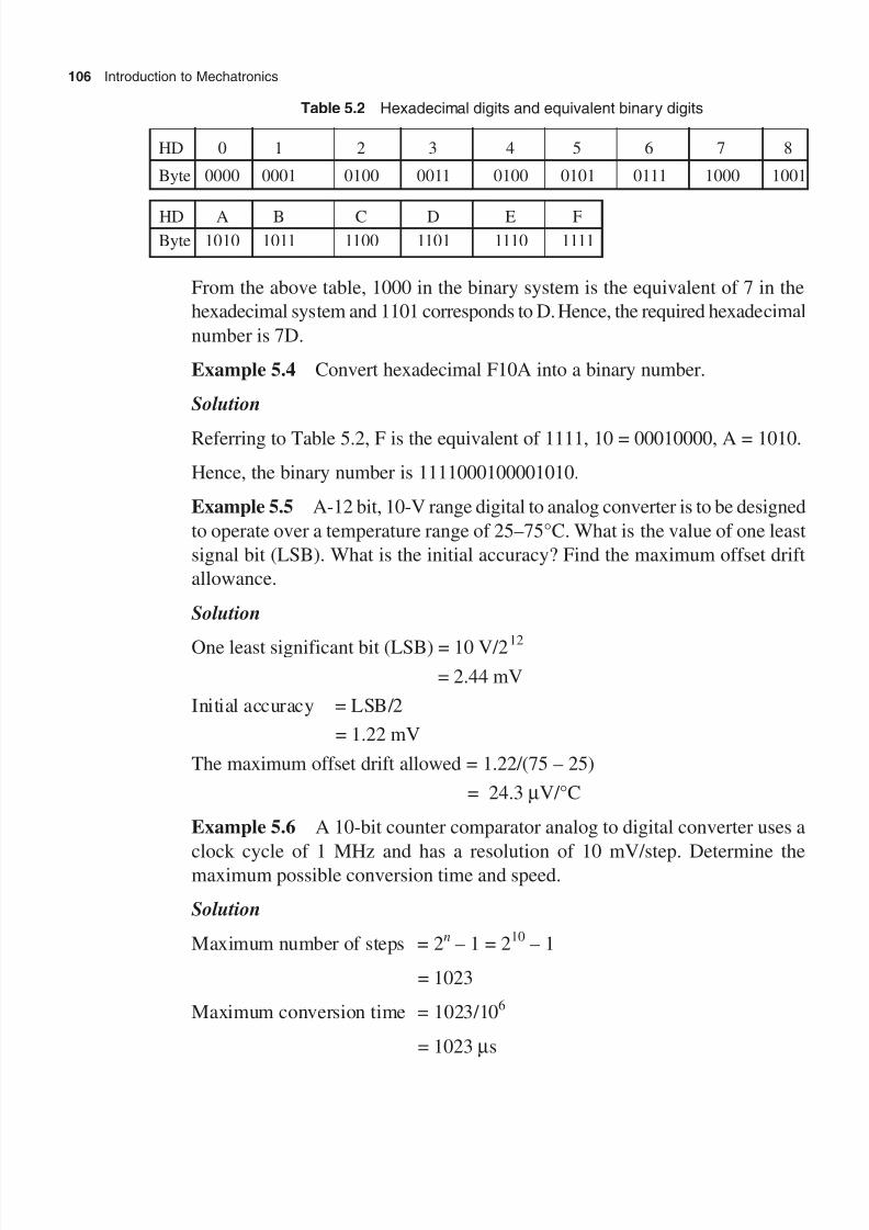
8/11/2019 Introduction to Mechatronics - Appuu Kuttan.pdf
http://slidepdf.com/reader/full/introduction-to-mechatronics-appuu-kuttanpdf 115/345
106 Introduction to Mechatronics
Table 5.2 Hexadecimal digits and equivalent binary digits
HD 0 1 2 3 4 5 6 7 8
Byte 0000 0001 0100 0011 0100 0101 0111 1000 1001
HD A B C D E FByte 1010 1011 1100 1101 1110 1111
From the above table, 1000 in the binary system is the equivalent of 7 in the
hexadecimal system and 1101 corresponds to D. Hence, the required hexadecimal
number is 7D.
Example 5.4 Convert hexadecimal F10A into a binary number.
Solution
Referring to Table 5.2, F is the equivalent of 1111, 10 = 00010000, A = 1010.
Hence, the binary number is 1111000100001010.
Example 5.5 A-12 bit, 10-V range digital to analog converter is to be designed
to operate over a temperature range of 25–75°C. What is the value of one least
signal bit (LSB). What is the initial accuracy? Find the maximum offset drift
allowance.
Solution
One least significant bit (LSB) = 10 V/212
= 2.44 mV
Initial accuracy = LSB/2
= 1.22 mV
The maximum offset drift allowed = 1.22/(75 – 25)
= 24.3 mV/°C
Example 5.6 A 10-bit counter comparator analog to digital converter uses a
clock cycle of 1 MHz and has a resolution of 10 mV/step. Determine the
maximum possible conversion time and speed.
Solution
Maximum number of steps = 2n – 1 = 210
– 1
= 1023
Maximum conversion time = 1023/106
= 1023 ms

8/11/2019 Introduction to Mechatronics - Appuu Kuttan.pdf
http://slidepdf.com/reader/full/introduction-to-mechatronics-appuu-kuttanpdf 116/345
Computing Elements in Mechatronics 107
Maximum speed of conversion = 1/1023
= 997 bits/sec
Example 5.7 For an ADC with n = 3, R f = R = 6 k W, the input voltage scale is
0–10 V and V r = 5 V. (a) Calculate the full-scale range and nominal scale. (b)
Calculate resolution. (c) Calculate the amplification gain using an inverting
amplifier for signal conditioning, assuming that voltage output from a
piezoceramic transducer can be up to 500 V.
Solution
We have V fsr = 2 R f V R / R = 10 V = V N
Resolution, r = V N /2n = 10/8 = 1.25 V
A gain of 10/500 = 0.02 reduces the maximum voltage 500 V to 10 V, achieving
an ideal matching of the domain of the input voltage from 0 to 500 V, with the0 to 10 V ADC scale
Example 5.8 A 12-bit weighted resistor DAC has R f = 5 k W, V R = 5 V, and
R = 5 k W. Calculate the value of V o for (a) the least significant bit, (b) the most
significant bit, (c) the maximum value of the digital input, (d) the output for
binary input 100010010001, and (d) the full-scale range voltage V fsr.
Solution
For LSB, the binary input is 000000000001 such that V oLSB
= –2(5)(1/212
)
= – 0.00244 V = 2.44 mV.
The resolution is also 2.44 mV.
For MSB, the binary input is 100000000000, V oMSB = –2(5)(1/21) = – 5 V.
The maximum value of the digital input is 111111111111 such that
V o = –2(5)1
2
2
29 999756
1 12+º+
= – . V
For the binary input 100010010001,
V o = –2(5)1
2
1
2
1
2
1
21 5 8 12+ + +
= – 5.35 V
V fsr = 2 R f V R / R = 10 V
Example 5.9 Design a circuit using an op-amp for weighing soap cakes in a
soap manufacturing company. The machine is to be designed to sense 2N weights,
1 N weights, and zero weight. LED2 lights when 2N weight is present, and
LED1 lights when 1N weight is present and at zero weight.
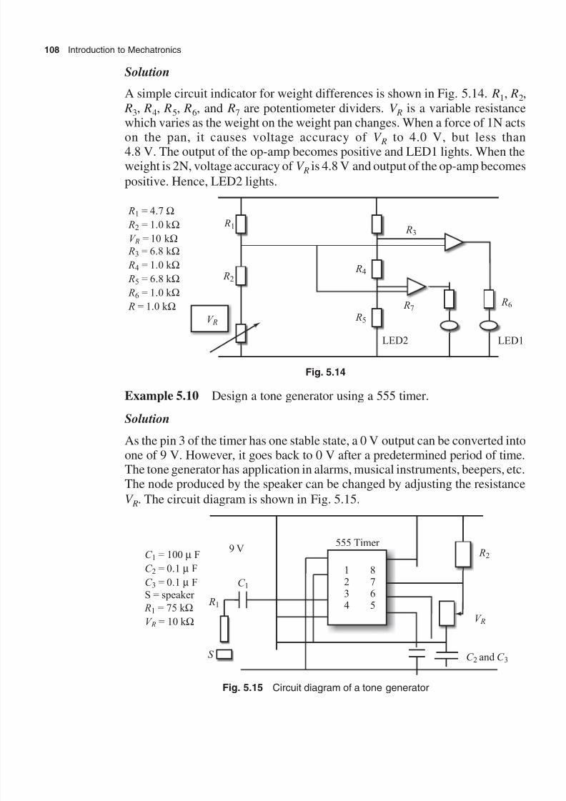
8/11/2019 Introduction to Mechatronics - Appuu Kuttan.pdf
http://slidepdf.com/reader/full/introduction-to-mechatronics-appuu-kuttanpdf 117/345
108 Introduction to Mechatronics
Solution
A simple circuit indicator for weight differences is shown in Fig. 5.14. R1, R2,
R3, R4, R5, R6, and R7 are potentiometer dividers. V R is a variable resistancewhich varies as the weight on the weight pan changes. When a force of 1N acts
on the pan, it causes voltage accuracy of V R to 4.0 V, but less than4.8 V. The output of the op-amp becomes positive and LED1 lights. When theweight is 2N, voltage accuracy of V R is 4.8 V and output of the op-amp becomes
positive. Hence, LED2 lights.
V R
R1
R2
R4
R5
R3
R7
LED2
R6
LED1
R
R
V
= 4.7
= 1.0 k
= 10
W
W
W
1
2
R k
R
R
R R
R
3 = 6.8
= 1.0
= 6.8= 1.0
= 1.0
W
W
WW
W
4
5
6
k
k
k k
k
Fig. 5.14
Example 5.10 Design a tone generator using a 555 timer.
Solution
As the pin 3 of the timer has one stable state, a 0 V output can be converted intoone of 9 V. However, it goes back to 0 V after a predetermined period of time.The tone generator has application in alarms, musical instruments, beepers, etc.The node produced by the speaker can be changed by adjusting the resistance
V R. The circuit diagram is shown in Fig. 5.15.
1234
8765
555 Timer R2
V R
C 2 and C 3
R1
S
C 1
9 VC
C
C
R
V
= 100 F
= 0.1
= 0.1
S = speaker
= 75
= 10
m
W
W
12
1
3
R
m
m
F
F
k
k
Fig. 5.15 Circuit diagram of a tone generator

8/11/2019 Introduction to Mechatronics - Appuu Kuttan.pdf
http://slidepdf.com/reader/full/introduction-to-mechatronics-appuu-kuttanpdf 118/345
Computing Elements in Mechatronics 109
Example 5.11 Sketch a block diagram for the temperature control of a heater
using a PLC.
Solution
The input corresponding to temperature could be a thermocouple output, which
after amplification can be fed to the analog to digital converter into the PLC.
The PLC is programmed to give an output proportional to the error from the
reference temperature and measured temperature. The output is then fed through
a digital to analog converter to actuate the heater in order to reduce the error.
Amplifier
Thermocoupleinput
ADC PLC DAC
Buffer
Heater
+ V
Fig. 5.16 Temperature control of heater with PLC
Exercises
5.1 Differentiate between analog and digital computers.
5.2 Generate an analog computer solution for the differential equation
d x
dy
dx
dt x
2
25 8+ + = 10 sin t
5.3 Explain the working of A/D and D/A converters.
5.4 Explain the structure of an 8085 microprocessor.
5.5 Explain the function of a microprocessor.
5.6 What are the advantages of the PLC over the microprocessor?
5.7 Explain a ladder diagram with an example.
5.8 Explain different storage devices used in computers.
5.9 Explain the working of a three-dimensional digitizer.
5.10 Explain the working of a dot matrix printer.

8/11/2019 Introduction to Mechatronics - Appuu Kuttan.pdf
http://slidepdf.com/reader/full/introduction-to-mechatronics-appuu-kuttanpdf 119/345
Systems Modelling and Analysis
A control system is a set or collection of things working in close coordination toprevent a system from giving undesirable output or performance. The system
can be natural or man-made. It can have input and output. A control system isalso used to control the output of a system to some particular value or particularsequence of values. A control system has a controller, which gives a manipulated
variable input to achieve control over the output. There are two basic forms ofa control system: one being open-loop system and the other being closed-loopsystem. Open-loop systems have the advantage of being relatively simple andconsequently low cost with generally good reliability. However, these systemsare often inaccurate, since there is no correction for errors. Closed-loop systemshave the advantage of being relatively accurate in matching the actual input to
the required values. However, they are complex and hence costly. Closed-loopcontrol systems are sensitive to disturbance, instability, response speed, andparameter variation. Any fluctuations of these values should be suitably
responded to by the system to ensure that the output quality is maintained without
any error.
An unstable system can be made stable and its response speed brought to
satisfactory levels with the help of a feedback control system. Similarly, any
variation in the parameters of system elements should not affect the accuracy of
the output. Figure 6.1(a) graphically illustrates a system and Figs 6.1(b) and (c)
illustrate control systems of open-loop and closed-loop type, respectively.
A fan with regulator can be considered as an open-loop system. The control
knob positions of the regulator give the various desired speeds of the fan and
the regulator acts as a controller that manipulates voltage as a variable parameter
to exercise control over the speed of the fan. Depending on the voltage input to
the fan motor, the fan rotates at a different speed. The occupants of the room
can adjust the regulator knob to make the fan run at a desired speed. This system
acts as manual, closed-loop system.
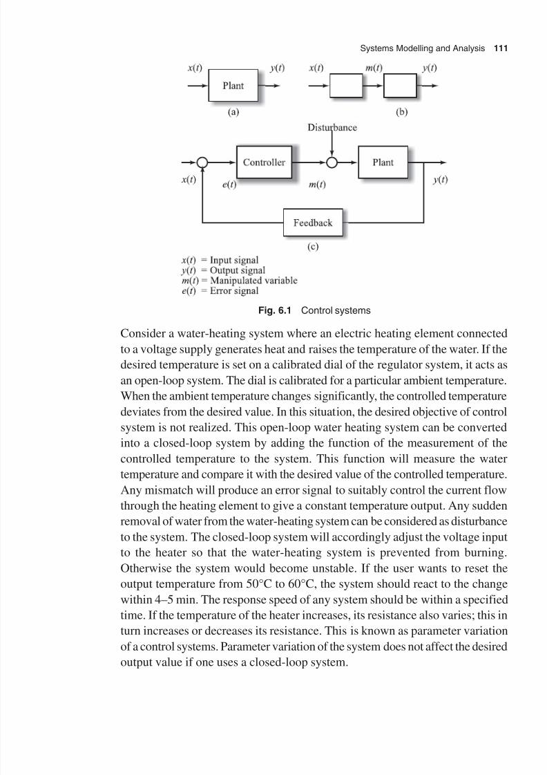
8/11/2019 Introduction to Mechatronics - Appuu Kuttan.pdf
http://slidepdf.com/reader/full/introduction-to-mechatronics-appuu-kuttanpdf 120/345
Systems Modelling and Analysis 111
Fig. 6.1 Control systems
Consider a water-heating system where an electric heating element connected
to a voltage supply generates heat and raises the temperature of the water. If the
desired temperature is set on a calibrated dial of the regulator system, it acts as
an open-loop system. The dial is calibrated for a particular ambient temperature.
When the ambient temperature changes significantly, the controlled temperature
deviates from the desired value. In this situation, the desired objective of control
system is not realized. This open-loop water heating system can be converted
into a closed-loop system by adding the function of the measurement of the
controlled temperature to the system. This function will measure the water
temperature and compare it with the desired value of the controlled temperature.
Any mismatch will produce an error signal to suitably control the current flow
through the heating element to give a constant temperature output. Any sudden
removal of water from the water-heating system can be considered as disturbance
to the system. The closed-loop system will accordingly adjust the voltage inputto the heater so that the water-heating system is prevented from burning.
Otherwise the system would become unstable. If the user wants to reset the
output temperature from 50°C to 60°C, the system should react to the change
within 4–5 min. The response speed of any system should be within a specified
time. If the temperature of the heater increases, its resistance also varies; this in
turn increases or decreases its resistance. This is known as parameter variation
of a control systems. Parameter variation of the system does not affect the desired
output value if one uses a closed-loop system.
8/11/2019 Introduction to Mechatronics - Appuu Kuttan.pdf
http://slidepdf.com/reader/full/introduction-to-mechatronics-appuu-kuttanpdf 121/345
112 Introduction to Mechatronics
6.1 Control System Concept
A control system is a set of elements or blocks, interconnected in such a way as
to help achieve some desired end. A study of the system consists of modelling,
analysis, and optimization. Modelling is the first step in the study of a system.
A system model is very useful for analysis, simulation, and designing of arequired system.
6.1.1 Classification of Systems
Systems are classified in a number of ways. There are causal and non-causal
systems, physical and non-physical systems, static and dynamic systems, linear
and non-linear systems, continuous data and discrete data systems, deterministic
and stochastic control systems, and lumped parameters and distributed
parameters systems.Cause-and-effect relationship is very common in nature. Systems governed by
such a relationship are called causal systems. Such relationships are alternatively
called input–output or stimulus–response relations. Examples of this type of
relationship are as follows:
1. Newton’s second law of motion, which gives acceleration equal to force
divided by mass.
2. Hook’s law, which gives displacement equal to force divided by stiffness.
3. Ohm’s law, which gives current equal to voltage divided by resistance.4. Bernoulli's law, which gives outflow equal to the area of the flow multiplied
by velocity.
All the causal systems can be represented as cause-and-effect relationships. On
the other hand, systems which do not obey the cause-and-effect relationship are
said to be non-causal. Typically, such systems are anticipatory in nature. For
example, stock market speculation, chess game played between a human and
computer, and the sixth sense (of human in danger) are all examples of non-
causal response.
A physical system comprises physical elements such as springs, valves, gear
trains, capacitors, batteries, etc. On the other hand, there are systems which
have no physical existence. Even the components of such systems do not have
any existence in this material and physical world. Such systems are non-physical
systems. Systems of philosophy, mathematical logic, etc. are typical examples
of non-physical systems.
A static system is one that does not change with time. Such systems are governed
by algebraic equations. Systems following Ohm’s law or Hook’s law are static

8/11/2019 Introduction to Mechatronics - Appuu Kuttan.pdf
http://slidepdf.com/reader/full/introduction-to-mechatronics-appuu-kuttanpdf 122/345
8/11/2019 Introduction to Mechatronics - Appuu Kuttan.pdf
http://slidepdf.com/reader/full/introduction-to-mechatronics-appuu-kuttanpdf 123/345
114 Introduction to Mechatronics
a rocket changes with time due to the continuous depletion of fuel and reduction
in gravitational force as the rocket moves away from the earth. The complexity
of the control system design increases considerably if the parameters are time
varying.
6.1.2 Modelling of Systems
Modelling is the first step in the study of a system. It enables one to understand
the construction and operation of a system. It helps to analyse the behaviour of
the system under various operating conditions. A model is defined as a
representation of some or all characteristics or aspects of the behaviour of a
system or a device or an object.
There are basically three types of models: mathematical, physical, and logical.
Mathematical models may be linear or non-linear, static or dynamic, continuousor discrete data, deterministic or stochastic. Physical systems can be represented
in electrical analogs or scale model. Scale models can be made for network
analysis, aircraft and vessels, dams and valleys, buildings and townships, etc.
Logical system models may be heuristic or computational. A computer can be
used for modelling logical systems. Mathematical models consist of equations
or mathematical expressions describing the principle of operation and
characteristics of the components, elements, or the entire systems. Such
mathematical expressions are obtained by applying the basic laws of physics
such as Newton’s laws of motion, the principle of conservation of energy,momentum and mass, the laws of thermodynamics, Faraday’s laws of
electromagnetic induction, Ohm's and Coulomb’s laws, etc.
Dynamic systems can be modelled by differential equations. The governing
differential equations can be solved by classical solutions by determining the
complimentary function and particular integral, or by an analog computer, or
by the Laplace transform technique. The first two methods are time consuming,
whereas in the Laplace domain the differential equation can be simplified very
easily to solve the problem. In the classical control approach the transfer function
concept is used to obtain the output response. Transfer function is defined as
the ratio of the Laplace transform of the output to the Laplace transform of the
input, assuming all the initial conditions are zero. The transfer function concept
of design can be applied only for the linear, time-invariant and single-input–
single-output (SISO) system. In the modern control theory, a system is
represented through a state-space representation. The state-space representation
of a system permits to consider initial values. It can be applied to multiple-
input–multiple-output (MIMO) systems. Moreover, the state-space
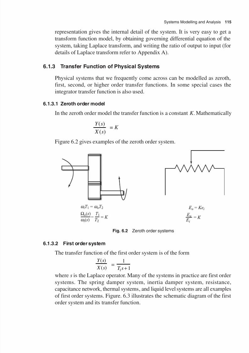
8/11/2019 Introduction to Mechatronics - Appuu Kuttan.pdf
http://slidepdf.com/reader/full/introduction-to-mechatronics-appuu-kuttanpdf 124/345
Systems Modelling and Analysis 115
representation gives the internal detail of the system. It is very easy to get a
transform function model, by obtaining governing differential equation of the
system, taking Laplace transform, and writing the ratio of output to input (for
details of Laplace transform refer to Appendix A).
6.1.3 Transfer Function of Physical Systems
Physical systems that we frequently come across can be modelled as zeroth,
first, second, or higher order transfer functions. In some special cases the
integrator transfer function is also used.
6.1.3.1 Zeroth order model
In the zeroth order model the transfer function is a constant K . Mathematically
Y s X s
( )( )
= K
Figure 6.2 gives examples of the zeroth order system.
Fig. 6.2 Zeroth order systems
6.1.3.2 First order system
The transfer function of the first order system is of the form
Y s
X s
( )
( )=
1
11T s +
where s is the Laplace operator. Many of the systems in practice are first order
systems. The spring damper system, inertia damper system, resistance,
capacitance network, thermal systems, and liquid level systems are all examples
of first order systems. Figure. 6.3 illustrates the schematic diagram of the first
order system and its transfer function.
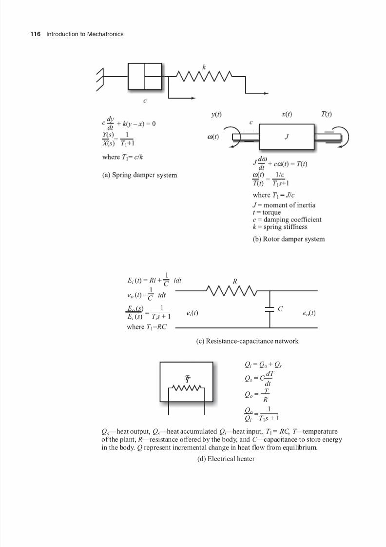
8/11/2019 Introduction to Mechatronics - Appuu Kuttan.pdf
http://slidepdf.com/reader/full/introduction-to-mechatronics-appuu-kuttanpdf 125/345
116 Introduction to Mechatronics
R
C e t o( )e t i( )
(c) Resistance-capacitance network
E t Ri idt
e t
i
o
( ) = +1
( ) =C 1
idt
E s E s T s
( )=
1
( ) + 1o
i i
where =T RC 1
C
T T
Q Q Q
Q C dT
dt Q T
R
QQ T s
i o s
s
o
o
i
= +
=
=
=1
+ 11
Q Q Q T RC T R C Q
o —heat output, heat accumulated heat input, = , temperatureof the plant, esistance offered by the body, and capacitance to store energyin the body. represent incremental change in heat flow from equilibrium.
s i — — — —r —
1
(d) Electrical heater

8/11/2019 Introduction to Mechatronics - Appuu Kuttan.pdf
http://slidepdf.com/reader/full/introduction-to-mechatronics-appuu-kuttanpdf 126/345
Systems Modelling and Analysis 117
Fig. 6.3 First order systems
6.1.3.3 Second order system
The study of second order systems may be generalized by the introduction of a
certain parameter to the study of the first order systems. The transfer function
of a second order system in the canonical form is
Y s
X s T s T s
( )
( )=
+ +
1
1 11 2 = – ––V V ±
2
1
=1
2 12
2s s
n nω ς
ω + +
where T 1 and T 2 are time constants, w n is the natural frequency of the system,
and V is the damping ratio. It can be easily shown that
12w n
= T 1T 2
and
21 2
V
w nT T = +
Using the relationship ( ) – ( – )T T T T T T 1 22
1 22
1 24+ = , the time constants T 1 and
T 2 can be determined.
The spring-mass-damper system [block diagram shown in Fig. 6.4(a)] and
resistance-inductance-capacitance network [block diagram shown in Fig. 6.4(b)]
are examples of second order systems.
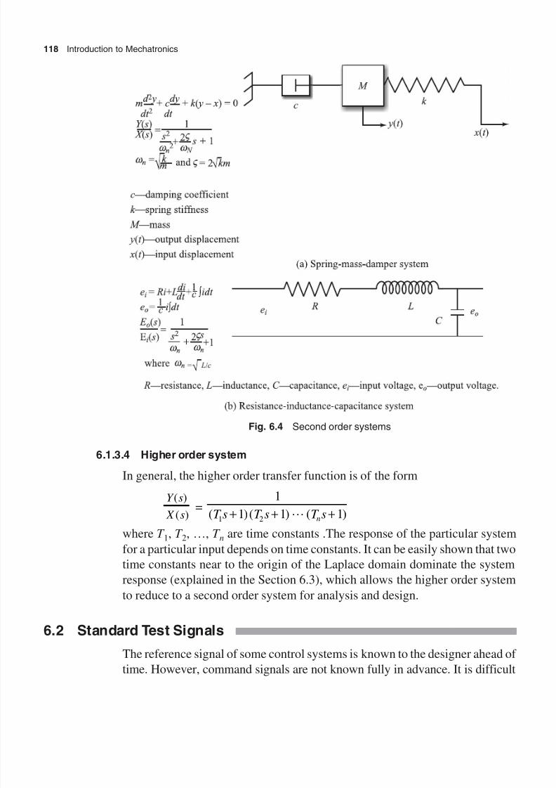
8/11/2019 Introduction to Mechatronics - Appuu Kuttan.pdf
http://slidepdf.com/reader/full/introduction-to-mechatronics-appuu-kuttanpdf 127/345
118 Introduction to Mechatronics
Fig. 6.4 Second order systems
6.1.3.4 Higher order system
In general, the higher order transfer function is of the form
Y s
X s
( )
( ) =
1
1 1 11 2( )( ) ( )T s T s T sn
+ + º +
where T 1, T 2, º, T n are time constants .The response of the particular system
for a particular input depends on time constants. It can be easily shown that twotime constants near to the origin of the Laplace domain dominate the system
response (explained in the Section 6.3), which allows the higher order system
to reduce to a second order system for analysis and design.
6.2 Standard Test Signals
The reference signal of some control systems is known to the designer ahead of
time. However, command signals are not known fully in advance. It is difficult

8/11/2019 Introduction to Mechatronics - Appuu Kuttan.pdf
http://slidepdf.com/reader/full/introduction-to-mechatronics-appuu-kuttanpdf 128/345
Systems Modelling and Analysis 119
to express the actual input signal mathematically by simple functions. The
characteristics of actual signals that severely strain a control system are listed
below:
1. A certain shock (impulse function)
2. A sudden change (step function)
3. Linear change with time (ramp function)
4. Faster change with time (parabolic function)
5. Sudden sinusoidal force input (sinusoidal function)
The dynamic behaviour of a system can be adequately judged and compared
under the application of standard test signals. Standard test signals are impulse,
step, ramp, parabolic, and sinusoidal inputs. If the input is sinusoidal, the
behaviour analysis is known as frequency domain analysis. For all other typesof input, the behaviour analysis is known as time domain analysis. Figure 6.5
illustrates different types of standard input signals in time scale and their
corresponding Laplace transforms.
Time Time
X t t t K t t
( ) = 0 for < 0( ) = for 0 < < X 1
X X
( ) = 0 for < 0( ) = for > 0t t t K t
X s e kdt k K ( ) = lim = lim = lim st e st t 1
1 – –e – –st [ [
0[ [ s
Applying L’ Hospital’s rule and limit,
( ) = X s K
(a) Pulse input (b) Step input
t 1
t t 1 0
X s e kdt ( ) = = 1 –st
0
t t 1
s
s
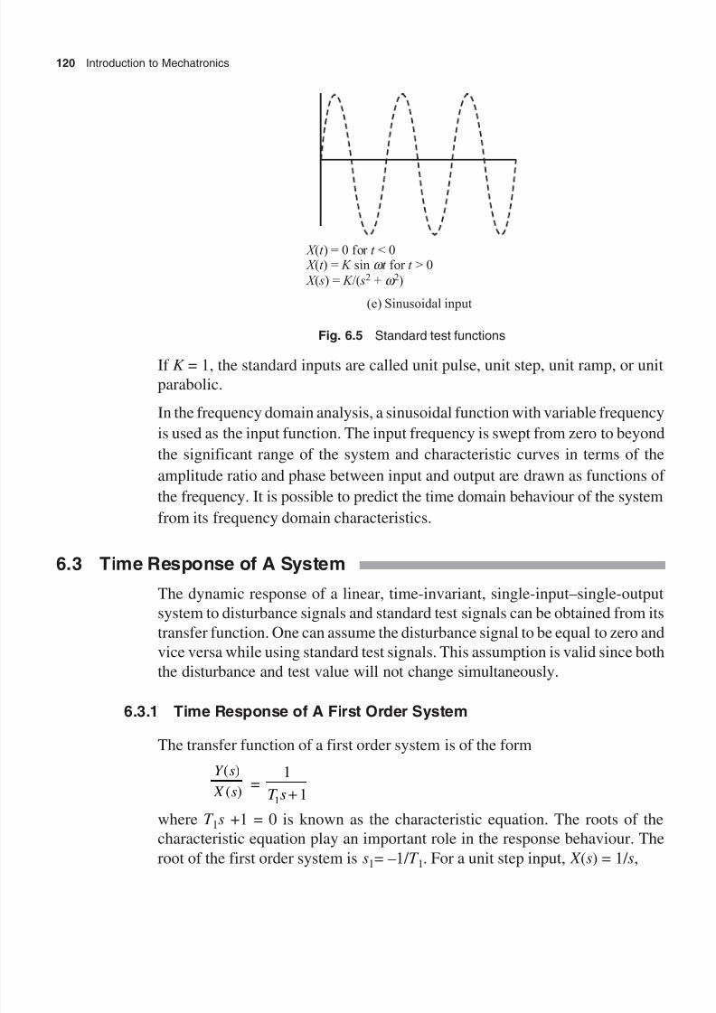
8/11/2019 Introduction to Mechatronics - Appuu Kuttan.pdf
http://slidepdf.com/reader/full/introduction-to-mechatronics-appuu-kuttanpdf 129/345

8/11/2019 Introduction to Mechatronics - Appuu Kuttan.pdf
http://slidepdf.com/reader/full/introduction-to-mechatronics-appuu-kuttanpdf 130/345
Systems Modelling and Analysis 121
Y (s) =1 1
11s T s +
y(t ) = L
s T s
L A
s
L B
T s
-
+
= +
+
1
1 1
1 1
1 1
–1 –1
where
A =1
11T s + at s = 0 (= 1)
and
B =1
sat s = –
1
1T (= –T1)
y(t ) = 11
− e t T – /
The response of y(t ) for unit step input is shown in Fig. 6.6(a). While y(t ) increases
exponentially as time increases, there is always a steady state error between input
and output. If the time constant is negative, the response will be y(t ) = K (–1 +
et T / 1 ), since the root of the characteristic equation is positive, +1/ T 1, which will
lead to an increase in the amplitude as the time lapses and the system will
become unstable. For the system to be stable, roots of the characteristic equation
should be a negative real number. Figure 6.6(b) shows the response for the
positive roots of the characteristic equation.
Similarly, the ramp response is obtained by substituting X (s) = K / s2. Then
Y (s) =1 1
121s T s + =
T
s
T
s
T
T s
1
2
12
12
1 1– +
+
Taking the term-by-term Laplace transform, one gets
y(t ) = T t T T et T
1 12
12 1– / +
The ramp response is shown in Fig. 6.6(c), wherein it is seen that y(t ) increases
linearly with time and there is a displacement lag or error of T 12 .

8/11/2019 Introduction to Mechatronics - Appuu Kuttan.pdf
http://slidepdf.com/reader/full/introduction-to-mechatronics-appuu-kuttanpdf 131/345
122 Introduction to Mechatronics
Fig. 6.6 Response of a first order system
6.3.2 Time Response of A Second Order System
The study of the second order system may be generalized since it is also
important for higher order systems. A higher order system can also be reduced
to a second order system and the response of the reduced second order system
is almost the same as the higher order system. The canonical form of any
second order system is
Y s
X s
( )
( )=
1
1 1 2
1
211
2
2 2 2
2
( ) ( )T s T s s s sss
n
n n
n n
+ + =
+ + =
+ +
w
Vw w
w
V
w
The characteristic equation of a second order system can be represented as
s sn n2 22Vw w + = 0. The roots of the characteristic equation play an important role
in the response and depend on the damping ratio V . The roots of the characteristic
equation are as given below:
s1, 2 =–2 –
– –Vw V w w
w V V n n n
n
+= ±
4
21
2 2 2
2
There are five possible responses from the system depending on the value of V .
The five cases are as follows.
CASE 1: V = 0
If V = 0, the roots of the characteristic equation are a complex pair with only animaginary part. That is, s1,2 = ± j –w . For the unit step input X (s) = 1/ s,
y(t ) = Ls s
Ls
Ls
n
n
n
n
–1 –1 –1
( )
w
w
w
w
2
2 2
2
2 2
1
+
+ +
+
= 1–C sin w n t
where C is a constant. The response curve is shown in Fig. 6.7.

8/11/2019 Introduction to Mechatronics - Appuu Kuttan.pdf
http://slidepdf.com/reader/full/introduction-to-mechatronics-appuu-kuttanpdf 132/345
Systems Modelling and Analysis 123
Fig. 6.7 Sinusoidal oscillation
CASE 2: V > 1
When V >1, the system is said to be over-damped. In this case the roots of the
characteristic equation are real and different. Roots are s1,2 = w n – –
–
ς ς ±
2
1 .For the unit step input X (s) = 1/ s and taking inverse Laplace transform,
y(t ) = 1 1 21 2- C e C e
s t s t –
where C 1 = s2 /(s2 – s1) and C 2 = s1 /(s2 – s1) are constants and s1 and s2 are the
roots of the characteristic equation. Its response curve is shown in Fig. 6.8.
Fig. 6.8 Over-damped response
CASE 3: V = 1
The roots are real and equal in this case. This system is known as a critically
damped system. The root is s1 = –V w n. For unit step input X (s) = 1/ s and taking
inverse Laplace transform of Y (s),
y(t ) = 1– ––e ten nt
n
t w w w
The response curve for this case is shown in Fig. 6.9.
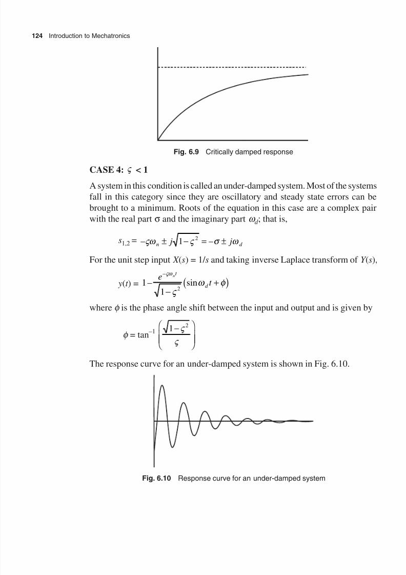
8/11/2019 Introduction to Mechatronics - Appuu Kuttan.pdf
http://slidepdf.com/reader/full/introduction-to-mechatronics-appuu-kuttanpdf 133/345
124 Introduction to Mechatronics
Fig. 6.9 Critically damped response
CASE 4: V < 1
A system in this condition is called an under-damped system. Most of the systems
fall in this category since they are oscillatory and steady state errors can bebrought to a minimum. Roots of the equation in this case are a complex pair
with the real part s and the imaginary part w d ; that is,
s1,2 = – –Vw V s w n d j j± - = ±1 2
For the unit step input X (s) = 1/ s and taking inverse Laplace transform of Y (s),
y(t ) = 11
2– sin
–e
t nt
d
ςω
ς ω φ
−+
where f is the phase angle shift between the input and output and is given by
f = tan–1 1 2-
V
V
The response curve for an under-damped system is shown in Fig. 6.10.
Fig. 6.10 Response curve for an under-damped system

8/11/2019 Introduction to Mechatronics - Appuu Kuttan.pdf
http://slidepdf.com/reader/full/introduction-to-mechatronics-appuu-kuttanpdf 134/345
Systems Modelling and Analysis 125
CASE 5: V is negative
Consider an under-damped system with a negative damping ratio. The roots of
the characteristic equation have a positive real part with a complex pair. That is,
s1,2 = + ± - = ±Vw V s w n d j j1 2 –
For step input X (s) = K /s,
y(t ) = 11 2
– sine
t nt
d
+
−+
ςω
ς ω φ
The response grows positively as the time lapses and the system collapses as
the amplitude increases beyond a limiting value. Hence, for stability, the roots
of the characteristic equation should be a negative real number or complex pair
with a negative real part. The response curve for this case is shown in Fig. 6.11.
Fig. 6.11 Response curve for positive roots
6.3.3 Characteristics of an Under-damped System
The study of the control system in time domain essentially involves the equation
of transient and steady state response of the system. The nature of the transient
response of the linear control system is revealed by any of the standard test
signals. Step signal is usually used for the analysis of the transient response as
well as the steady state response. The steady response depends on both thesystem and the type of input.
The transient response of an under-damped system exhibits damped oscillation
before reaching the steady state. The transient response characteristic of an
under-damped system for step input is commonly specified by the rise time T r ,
delay time T d , peak time T p, peak overshoot M p, and settling time T s (see Fig.
6.12). The rise time T r is the time required to raise the response from 10% to
90% of the input value. The peak time T p is the time required to raise the response
to the overshoot level. The settling time T s is the time required to settle the
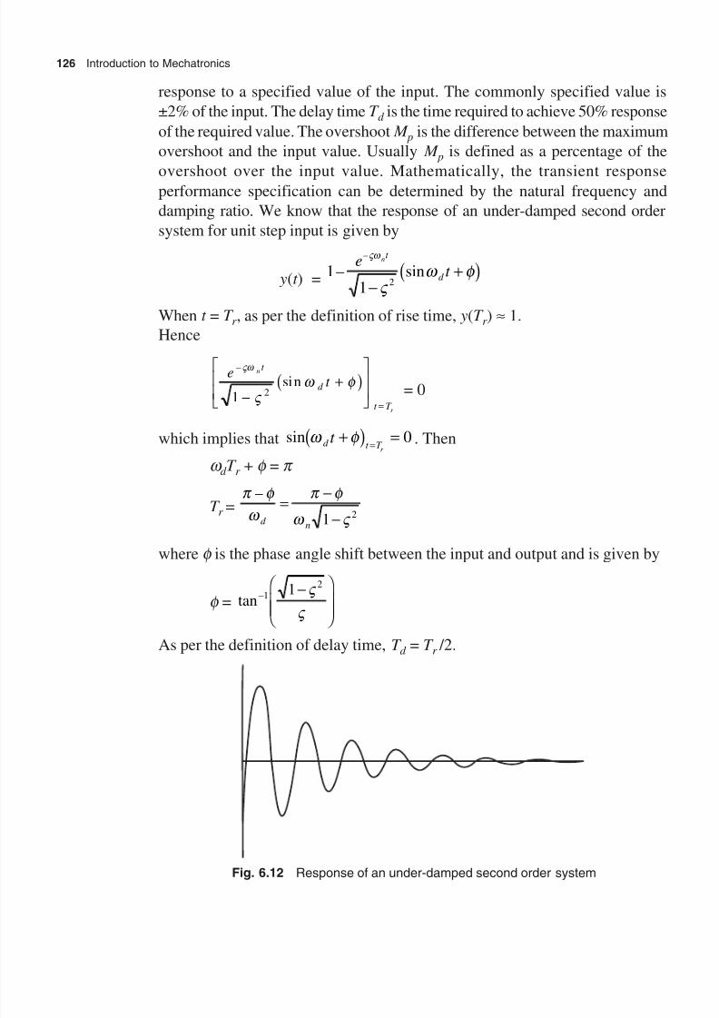
8/11/2019 Introduction to Mechatronics - Appuu Kuttan.pdf
http://slidepdf.com/reader/full/introduction-to-mechatronics-appuu-kuttanpdf 135/345
126 Introduction to Mechatronics
response to a specified value of the input. The commonly specified value is
±2% of the input. The delay time T d is the time required to achieve 50% response
of the required value. The overshoot M p is the difference between the maximum
overshoot and the input value. Usually M p is defined as a percentage of the
overshoot over the input value. Mathematically, the transient responseperformance specification can be determined by the natural frequency and
damping ratio. We know that the response of an under-damped second order
system for unit step input is given by
y(t ) =1
12
– sin–
et
nt
d
ςω
ς ω φ
−+
When t = T r , as per the definition of rise time, y(T r ) ª 1.
Hence
et
n
r
t
d
t T
–
sinVw
V w f
1 2-+
=
= 0
which implies that sin w f d t T t
r
+ == 0 . Then
w d T r + f = p
T r =p f
w
p f
w V
–
d n
= -
-1 2
where f is the phase angle shift between the input and output and is given by
f = tan–1 1 2-
V
V
As per the definition of delay time, T d = T r /2.
Fig. 6.12 Response of an under-damped second order system
8/11/2019 Introduction to Mechatronics - Appuu Kuttan.pdf
http://slidepdf.com/reader/full/introduction-to-mechatronics-appuu-kuttanpdf 136/345
Systems Modelling and Analysis 127
The peak time T p occurs when response reaches its maximum value. Hence,
dy
dt = 0
or Vw V
w f V
w f w Vw Vw f
n
t
d
t
d d
T T
et
et
n d
p
1 10
2 2–
sin – (cos )–
+-
+
=+
=
That is,
Vw w f w w f n d d d T T t
p
sin – cos( )+ +=
= 0
Since f = tan–1 1 2-
V
V
,
sin f = 12
– ς
and cos f = V
Also w d = 12
– ς
So w f w f f w f n d d T T t
p
cos sin – sin cos( )+ +=
= 0
sinw d T p = 0
T p =p
w
p
w V d n
=2 1–
Maximum overshoot M p = y(T p) – x (T p).
y(T p) – 1 = – sine
T n pT
d p
-
-+
Vw
V w f
1 2
Substituting
T p =p
w
p
w V d n
=2 1–
we get
M p =e
– /( – )
–sin
Vp V
V p f
1
2
2
1+ =
e– / ( – )
–sin
Vp V
V f
1
2
2
1

8/11/2019 Introduction to Mechatronics - Appuu Kuttan.pdf
http://slidepdf.com/reader/full/introduction-to-mechatronics-appuu-kuttanpdf 137/345
128 Introduction to Mechatronics
Since sin f = 1 2– ς ,
M p = e– /( – )Vp V 1 2
Percentage overshoot is
y T x T
x T
p p
p
( ) – ( )
( )¥ 100% = e
– /( – )Vp V 1 2
%
V 2 = ( ) / ( )ln M M p p2 2 2
ln + p
Table 6.1 shows the percentage of overshoot for various values of the damping
ratio. Table 6.1 Overshoot versus damping ratio
% Overshoot Damping ratio
100 0
80 0.1
60 0.2
40 0.3
20 0.510 1.0
By the definition of settling time, the amplitude of the output y(t ) is equal to
0.95 for a 5% of the tolerance band. That is,
11
2–
–
–e n
p
t
t T
Vw
V
=
= 0.95
T s =1
Vw n ln 0 05 1 2. – V
A common design practice is to approximate the settling time to four times the
time constant, which gives a tolerance band of 2%.That is
T s =4
0 08Vw
V n
, .£ £

8/11/2019 Introduction to Mechatronics - Appuu Kuttan.pdf
http://slidepdf.com/reader/full/introduction-to-mechatronics-appuu-kuttanpdf 138/345
Systems Modelling and Analysis 129
6.3.4 Steady State Response
In specifying the steady state response characteristic of the system, it is common
to specify the steady state error of the system to one or more of the standard test
signals. The steady state error e ss indicates the error between the actual output
and the desired output as time t tends to infinity. Mathematically,
e ss =lim ( ) – ( )t
x t Y t Æ•
e ss = lim ( ) – ( )s
s x s Y sÆ0
The second equation is obtained by using the mean value theorem. When the
response is considered for disturbance x (s) = 0, e ss = lim ( ).s
sY s→0
The steady state
error for a second order under-damped system for the step input is
e ss = lim ( ) lim sin –t t
t
d y t e
t n
Æ• Æ•- =
-=1
10
2
Vw
V w f
For unit ramp input x (s) = 1/ s2, the response of a second order system is
y(t ) = t t
t n
n
d --
2
1 2
Vw
w V w f sin –
Its steady state error is
e ss = lim ( )t
n
t y t Æ•
- =2V
w
An important step is that the best value of the damping ratio should be chosen
for any control system for better performance of a mechatronic system. A smaller
damping ratio decreases the rise time, but increases the peak overshoot. Many
systems are designed for a damping ratio in the range of 0.4 to 0.7. If rise timeconsiderations allow, V close to 0.7 is the most obvious choice because it results
in a minimum normalized settling time. If the requirement is to design an
extremely accurate control system whose steady state errors are extremely small,
the damping ratio should be as small as possible. Because the steady state error
is proportional to the damping ratio, values close to 0.1 are not reasonable for
such applications. Disadvantages of a relatively long settling time have to be
tolerated. A good compromise between rise time and overshoot is V = 1.

8/11/2019 Introduction to Mechatronics - Appuu Kuttan.pdf
http://slidepdf.com/reader/full/introduction-to-mechatronics-appuu-kuttanpdf 139/345
130 Introduction to Mechatronics
6.3.5 System Type Number
The difference between the input signal x (t ) and output y(t ) is the error signal
e(t ). For a stable system, the transient component of response e(t ) will essentially
die away, leaving only the steady state component. The steady state error then is
given by
e ss = lim [ ( ) ( )] lim ( )( )
( )s ss x s y s sx s
Y s
X sÆ Æ- = -
0 0
1
Y (s)/ X (s) is the open-loop transfer function of the closed-loop system, which is
of the form
Y s
X s
( )
( )
=
K s Z
s s P
ii
m
N ii
m
( )
( )
+
+
’
’The term 1/ s N corresponds to N number of pure integration. If N = 0, the system
is called type zero system; if N is equal to1, the system is called type 1 system;
and if N is equal to 2, the system is called type 2 system. When s takes the value
of Z i (i = 1, 2, 3, …, m), the transfer function goes to zero. Such values are called
zeros of the system. Zeros are indicated as ‘0’. When s takes the values of – Pi
(i = 1, 2, …, n), the transfer function goes to infinity. Such values are called
poles of the system and are denoted by ‘ x ’. Steady state errors for various system
numbers and input are given in Table 6.2. The addition of an integrator to the
system tends to decrease the steady state error. However, integrators have
destabilizing effects on the system. Thus, control system design is usually a
trade-off between the steady state accuracy and acceptable related stability.
Table 6.2 Steady state error for various system numbers
Steady state error
Type of input Type 0 Type 1 Type 2
Unit step Finite 0 0
Unit ramp Infinite Finite 0
Unit parabolic Infinite Infinite 0
6.4 Block Diagram Manipulation
Consider the feedback control system shown as a block diagram in Fig. 6.13.
The transfer function of the system is indicated by G1(s), the transfer of the
controller is indicated by G2(s), and the feedback element transfer function is
H (s). Equation G(s) = G1(s) ¥ G2(s) is called the forward path transfer function
and H (s) is called the feedback path transfer function. G(s) ¥ H (s) is known as

8/11/2019 Introduction to Mechatronics - Appuu Kuttan.pdf
http://slidepdf.com/reader/full/introduction-to-mechatronics-appuu-kuttanpdf 140/345
Systems Modelling and Analysis 131
the open-loop transfer function of an open-loop system, whereas Y (s)/ X (s) =
G(s)/{1 + G H (s)} is called the open-loop transfer function of a closed-loop
system. Referring to Fig. 6.13, Y (s) = G(s) ¥ E (s), E (s) = X (s) – H (s) ¥ Y (s),
which gives Y (s)/ X (s) = G(s)/{1 +G H (s)}. The equation 1 + G(s) H (s) = 0 is
known as the characteristic equation.
G1( ) s G2( ) s
X s( ) Y s( )
H ( ) s
(a) Closed-loop system
Fig. 6.13 Block diagram of feedback control system
Control system analysis requires one to calculate the closed-loop transfer function
of a system through block diagram manipulation. The transfer function can be
obtained for each component of the system. It is important to note that a block
diagram can be connected in series only when the output of one block is not
affected by the next following block. If there is any loading effect between the
components, it is necessary to combine these components into a single block.
Any number of blocks representing non-loading components can be replacedby a single block. A complicated block diagram involving a feedback loop can
be simplified by a step-by-step rearrangement. Simplification of a block diagram
by rearrangement reduces the effort needed for subsequent mathematical analysis.
The simplification procedure for a block diagram is called block diagram
manipulation. The basic rules and guidelines for block diagram manipulation
are illustrated in Fig. 6.14. Adjusting the summing point or fixed point negative
feedback loop containing feedback H (s) will help to manipulate the block
diagram.

8/11/2019 Introduction to Mechatronics - Appuu Kuttan.pdf
http://slidepdf.com/reader/full/introduction-to-mechatronics-appuu-kuttanpdf 141/345
132 Introduction to Mechatronics
(a) Summing point moved forward
G s( ) H s( )
H s G s( ) ( )
H s( )
H s( )
G s( )G s( )
H s( )G s( )
(b) Fixed point moved backward
Fig. 6.14 Block diagram manipulation
6.5 Automatic Controllers
An automatic controller compares the actual value of the plant output with the
reference input to determine the deviation, if any, and produce a control signal
that will reduce the deviation to zero or to a smaller (negligible) value. The
manner in which the automatic controller produces the control signal is calledcontrol action. Industrial controllers are classified on the basis of their control
actions as follows:
1. Two-position or on-off controllers
2. Proportional controller
3. Integral controller
4. Proportional-plus-integral (PI) controller
5. Proportional-plus-derivative controller
6. Proportional-plus-integral-plus-derivative controller
In the two-position control system the actuating element has in many cases
simply on and off slots. On-off controllers are relatively simple and inexpensive.
Hence, they are widely used in industry and domestic control systems. The
output signal from this type of controller remains at a maximum or minimum
value, depending on the actuating error signal. Mathematically, m(t ) = m1 for
e(t ) > 0 and m(t ) = m2 for e(t ) < 0. The difference between m1 and m2 is known
as the differential gap.
8/11/2019 Introduction to Mechatronics - Appuu Kuttan.pdf
http://slidepdf.com/reader/full/introduction-to-mechatronics-appuu-kuttanpdf 142/345
Systems Modelling and Analysis 133
In a controller with proportional control action the relation between the output
of the controller is m(t ) = K P e(t ) and the transfer function is M (s)/ E (s) = K P,
where K P is the proportional gain which can be adjusted. The advantage of the
proportional controller is that it can bring the system to stability. However, a
steady state error is always present with the proportional controller.
In a controller with integral control action the value of the controller output
m(t ) is the integral of error signal. That is, m(t )= K I e t ( ) , where K I is an
adjustable constant called integral gain. The transfer function of the integral
controller is M (s)/ E (s) = K I / s. The advantage of the integral controller is that it
reduces the steady state error equal to zero, but the response is very slow due to
the integral action.
In a controller with derivative action the value of the controller output m(t ) is
changed at a rate proportional to the error signal. Mathematically,
–( )
( )
dm t
e t = K Ds
where K D is the derivative gain.
Proportional-plus-integral controllers bring the system to stability because of
their proportional action and the steady study state error for disturbance being
equal to zero due to integral action. However, there is some delay in response
due to the integral action. The controller action of a proportional-plus-integral
controller is defined by m(t ) = K Pe(t ) + K I Ú e(t )dt and the transfer function of the
controller is given by
M s
e s
( )
( ) = K P +
K
s
I
Proportional-plus-integral-plus-derivative (PID) controller is a combination of
proportional, integral, and derivative control actions. This combined action has
the advantage of the three individual control actions. The equation of a PID
controller with the combined action is given by
m(t ) = K P e(t ) + K I e t dt K
de t
dt D( )
( )
+ The transfer function of a PID controller is given by
M s
e s
( )
( ) = K P +
K
s
I + K Ds
where K P, K I , and K D are proportional gain, integral gain, and derivative gain,
respectively. The system becomes stable due to the proportional control action,
steady state error for disturbance being zero due to integral action, and the
8/11/2019 Introduction to Mechatronics - Appuu Kuttan.pdf
http://slidepdf.com/reader/full/introduction-to-mechatronics-appuu-kuttanpdf 143/345
134 Introduction to Mechatronics
correction of the error being faster due to the derivative action. However, the
PID controller is expensive.
Derivative controller action as an individual controller is not used since the
controller action is rate of error signal and hence the output is not going to
respond for error. For some industrial applications where tachogenerator outputis used for impact and jerk compensation, proportional-plus-derivative control
actions are used.
6.6 Frequency Domain Analysis
The phrase 'frequency response' means the steady state response of a system to
a sinusoidal input. In the frequency response method, the frequency of the output
signal varies over a certain range, keeping the amplitude constant. One advantage
of the frequency response is that it can use the data obtained from measurements
on a physical system without deriving its mathematical model. Frequency
response method was developed in 1930s and 1940s by Nyqist, Bode, Nicholas,
and others. It is the most powerful method in the classical control theory. The
Nyqist stability criterion enables us to investigate both absolute and relative
stabilities of a linear closed-loop system. In designing a closed-loop system,
one can adjust the frequency response characteristic of the open-loop transfer
function by using several design criteria in order to obtain an acceptable transient
response characteristic for the system. An example of input and output sinusoidal
signals is shown in Fig. 6.15. The frequency response of a stable, linear systemcan help configure the dynamic response to any form of input. Thus the control
system’s performance can be described in frequency response terms. The
correlation between transient response and frequency response through the
Fourier integral transform is an important basis of most design procedures and
criteria. Usually the Laplace domain behaviour is interpolated in terms of
frequency response characteristics, design in frequency domain and the frequency
response is then translated into the time domain.

8/11/2019 Introduction to Mechatronics - Appuu Kuttan.pdf
http://slidepdf.com/reader/full/introduction-to-mechatronics-appuu-kuttanpdf 144/345
Systems Modelling and Analysis 135
Fig. 6.15 Frequency response
6.7 Modern Control Theory
The current trend in engineering systems is greater design complexity. This has
been necessary to facilitate performance of complex tasks and help achievegood accuracy. Such complex systems may have multiple inputs and multiple
outputs and may be time varying. Because of the necessity to meet the increasing
stringent requirements on the performance of control systems such as turbo-jet
engines, nuclear power plants, there has been an increase in the system
complexity and the use of computers in the modern control theory. This has led
to a new approach to design and analyse control systems. Modern control theory
was developed around 1960. This approach is based on the concept of state
space and is applicable to linear and non-linear, time-varying systems. The state
variable approach is applicable to biological systems, economic systems, andsocial systems. Often, the state variables of a dynamic system are the variables
comprising a smallest set of variables that determine the state of a dynamic
system. State variables are represented as x 1, x 2, …, x n. If n state variables are
needed to completely describe the behaviour of the system, then these n states
can be considered as n components of a vector x . Such a vector is called state
vector. Any state can be represented by a point in the state space, where space is
an ‘n’-dimensional coordinate system. The state space analysis is concerned
with three types of variable that are involved in the modelling of a dynamic
8/11/2019 Introduction to Mechatronics - Appuu Kuttan.pdf
http://slidepdf.com/reader/full/introduction-to-mechatronics-appuu-kuttanpdf 145/345
136 Introduction to Mechatronics
system, namely, the input variable, output variable, and state variable. Let us
assume that a multiple-input–multiple-output system involves n integrator(s)
with m inputs and l outputs. The linear state equation for this is of the form
x ¢ = Ax + Bu
y = Cx + Eu
where x is the n ¥ 1 state vector, u is the m ¥ 1 input vector, y is the l ¥ 1 output
vector, and d is the n ¥ 1 disturbance vector. A is the n ¥ n state matrix, B is the
n ¥ m input matrix, C is the l ¥ n output matrix, and E is the n ¥ n disturbance
matrix.
6.7.1 State Space Equation of a System
The state space representation of a dynamic system can be obtained as illustrated
with the following example of the transfer function of a single-input–single-
output system.
( )
( )
Y s
X s = ( ) / ( )–b s b s b s b s a s a
n
i
n
n n
n n
n01
1 11
+ + … + + + + … +−
−
where X (s) is the single input and Y (s) is the single output and ai’s and bi’s are
constants. Partioning the transfer function,
Y s
X s
( )
( ) =
Y s s
s U s
( ) ( )
( ) ( )
x
x
The transfer function in the differential equation form is
u(t ) = ξ ξ ξ n n
nt a t a t ( ) ( ) ( )–+ + … +1
1
where the superscripts indicate the order of differentiation. Now define the state
variables as
x 1 = x (t )
x 2 = x 1• = x 1(t )
x n = x n–1
•
= x n– 1(t )
From this, we get
x n• = –an x 1 – an–1 x 2 – º – a1 x n
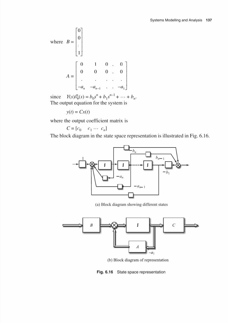
8/11/2019 Introduction to Mechatronics - Appuu Kuttan.pdf
http://slidepdf.com/reader/full/introduction-to-mechatronics-appuu-kuttanpdf 146/345
Systems Modelling and Analysis 137
where B =
0
0
1
A =
0 1 0 0
0 0 0 0
1 1
.
.
. . . . .
– – . . –a a an n-
since Y (s)/ x(s) = b0sn
+ b1sn–1
+ º + bn.
The output equation for the system is
y(t ) = Cx (t )where the output coefficient matrix is
C = [c0 c1 º cn]
The block diagram in the state space representation is illustrated in Fig. 6.16.
1
bn
bn 1
an
an 1
b1
(a) Block diagram showing different states
Fig. 6.16 State space representation

8/11/2019 Introduction to Mechatronics - Appuu Kuttan.pdf
http://slidepdf.com/reader/full/introduction-to-mechatronics-appuu-kuttanpdf 147/345
138 Introduction to Mechatronics
6.7.2 Transfer Function from State Space Representation
Correlation between the transfer function and the state space equation is
important. To derive the transfer function of a multiple-input–multiple-output
system, consider the following state space equation:
x ¢ = Ax + Bu
Y = Cx
Usually the state space representation of the system is indicated by the state
matrices triplet ( A, B, C ). For a change in the reset value, the disturbance vector
is assumed to be zero. Taking the Laplace transform of the state space equation,
sX (s) – AX (s) = BU (s), (sI – A) X (s) = BU (s)
Hence X (s) = (sI – A)–1
BU (s). Knowing X (s), the output vector Y (s) is
C (sI – A)–1
BU (s), that is,
Y (s) =W s
H sU s0
0
( )
( )( )
where W 0(s) is known as the numerator of the transfer function matrix C ,
adj (sI – A) B is of dimension ¥ m, H 0(s) is the open-loop characteristic
polynomial, which is equal to the determinant of (sI – A) = 0, and L–1
(sI – A) is
known as the transition matrix f (t ), which is equal to
e
At
= I At A
t
A
t
n L sI A
nn
+ + +…
+ =
22
2
–1
adj( – )
adj(sI – A) can be determined from the Leverier algorithm, which is equal to
I + CBs + CABs2 + º + CAn–1 Bsn–1
As in the classical control theory, the roots of the characteristic equation det
(sI – A) = 0 should be negative real numbers or complex numbers with negative
real parts. If the system is unstable or does not meet the specification, the system
can be brought to stability by applying the feedback law. If all the states are
available for feedback in the state space representation, then it is called state
feedback and all the poles of the system can be assigned arbitrarily.
6.7.3 Feedback Controller Design
The feedback law is used to bring an unstable system to stability,. The concepts
of controllability and observability play an important role in the design of a
controller in state space. The concepts of controllability and observability were
introduced by Kalman. The conditions of controllability and observability may
give the existence of a complete solution to the control system design problem.

8/11/2019 Introduction to Mechatronics - Appuu Kuttan.pdf
http://slidepdf.com/reader/full/introduction-to-mechatronics-appuu-kuttanpdf 148/345
Systems Modelling and Analysis 139
The solution to this problem may not exist if the system considered is not
controllable or observable. Although most of the physical systems are
controllable and observable, the mathematical model should be established.
A system is said to be controllable at a time t 0 if it is possible by means of an
unconstrained control vector to transfer the system from any initial state x (t 0)operator to any other state in some finite interval of time.
A system is sad to be observable at time t 0 if with the system in state x (t 0) it is
possible to determine this state from the observation of the output over a finite
time interval.
The solution to the state-space equation x ¢ = Ax + Bu is
x (t ) = e At
x (0) + e BU d At t t ( ) ( )
- t t t 0
where x (0) is the initial state at t = t 0 and t is the finite time interval t 0 < t < t .When time is required to final the state, applying the definition of complete
state of controllability,
x (t 1) = –e At
x (0) + e BU d At t t ( ) ( )- t t t
0
If the system is completely state controllable, then given the initial state
x (0) the above equation must be satisfied. This requires the rank of matrix
U = [ A AB … An–1
B] to have a full rank n. U is called the controllability matrix.
Considering the output equation of the state space representation, the output
vector is
y(t ) = Ce At
x (0)
If the system is completely observable, the output y(t ) over a time interval 0 < t
< t , x (0) is uniquely determined from the above equation. It can be shown that
it requires the rank of V = [(C T (CA)
T …(CA
n – 1)T ] to be a full rank. The matrix
V is called the observability matrix. The system should be controllable and
observable to design a controller and to bring the system to stability.For stability, the roots of the characteristic equation det(sI – A) = 0 should be
negative real numbers or a complex pair with a negative real part. Using the
state feedback law, all the roots of the characteristic equation can be placed
arbitrarily at desired locations. The design method to place the roots at desired
locations is called the pole placement or pole assignment technique. Consider a
controllable and observable linear system of the state space representation
( A, B, C ). Applying the feedback law u(t ) = v(t ) – K x (t ), where v(t ) is the
reference vector, the state space equation becomes

8/11/2019 Introduction to Mechatronics - Appuu Kuttan.pdf
http://slidepdf.com/reader/full/introduction-to-mechatronics-appuu-kuttanpdf 149/345
140 Introduction to Mechatronics
x = Ax + b[v(t ) – KCx (t )]
y = Cx
Taking the Laplace transform
(sI – A + BKC ) x (s) = Bv(s)Y (s) = Cx (s)
Then
X (s) = (sI – A + BKC )–1
Bv(s)
Y (s) = C (sI – A + BKC )–1 Bv(s)
Y (s) =W s
H sv s1
1
( )
( )( )
where W 1(s) = C adj(sI – A + BKC ), C is called the l ¥ m numerator transferfunction matrix of the closed-loop system and H 1(s) = det(sI – A + BKC ) = 0 is
the characteristic equation of the closed-loop system. By the proper choice of
m ¥ l coefficient of matrix K , the poles of the closed-loop system can be placed
arbitrarily. Since the characteristic equation is a non-linear equation, pole
assignment becomes difficult. Few iterative algorithms are available for pole
assignment. However, these algorithms do not guarantee the exact pole
placement. We now explain the linearization of the problem and equations for
the design of a controller.
Consider a closed-loop characteristic equation H 1(s) = det (sI – A + BKC ) = 0.
Assume the feedback in the dyadic form K = kf T , where k is the m ¥ 1 vector and
f T is the 1 ¥ l vector. The dyadic form is the outer product of two vectors. Hence
H 1(s) = |sI – A| | I + (sI – A) – 1 Bk f T C |
We use the determinant identity | I + ab | = 1 + ba, where a and b are vectors of
dimensions n ¥ 1 and 1 ¥ n, respectively. This is an inner product of two vectors.
H 1(s) = |sI – A| [1 + f T C (sI – A)–1 Bk ]
= H 0(s) + f T W 0(s)k
Assuming either vector f T
or k maximum of m or l poles can be assigned
arbitrarily. If the output coefficient matrix is an identity matrix, all the states of
the system are available for measurement. Then, assuming the vector k arbitrarily,
by the choice of the vector f T
, all the poles of the system can be assigned
arbitrarily. This pole assignment procedure is called state feedback. If all the
states are not available for measurement, this pole assignment procedure is
called the pole assignment with output feedback.
8/11/2019 Introduction to Mechatronics - Appuu Kuttan.pdf
http://slidepdf.com/reader/full/introduction-to-mechatronics-appuu-kuttanpdf 150/345
Systems Modelling and Analysis 141
6.8 Sequential Control System
There are many situations where control is exercised by items being switched
on or off at particular preset times or value in order to control the process and
give sequence of operations. For example, after step 1 is complete, step 2 starts,
and when step 2 is complete, step 3 starts, etc. The term ‘sequential control’ isused if control is such that control actions are strictly ordered in a time- or
event-driven sequence. Such a control could be obtained by an electrical circuit
with sets of relays and cam-operated switches, which are wired up in such way
as to give the required sequence of control actions. Such hard-cored circuits
have now been replaced by microprocessor-controlled systems, with the sequence
being controlled by a software program. For an illustration of sequential control,
consider the domestic washing machine, in which a number of operations are
carried out in a predetermined and prefixed sequence. These operations may
involve a pre-wash cycle, wherein the clothes in the drum are given a wash incold water, followed by the main wash cycle. The main wash cycle involves a
washing operation in hot water, a rinse operation (wherein clothes are rinsed in
cold water a number of times), and a spin operation (which removes water from
the clothes). Each of these operations involves a number of steps. The operating
sequence is called a program and the sequence of instructions in each program
is defined and built into the controller unit. As an another example, consider an
aircraft turbine engine, for which it is necessary to achieve maximum thrust
with a minimum engine weight. All components should operate at mechanical
or thermal limit for all the engines at critical operating engine conditions. Theoperating conditions depend on the speed of the aircraft as also the altitude of
the flight. Depending on the operating conditions, control parameters have to
set sequentially to control each limiting parameter and limit the engine thrust
so that none of the limits is exceeded. In the most recent design methods, the
military aircraft use multi-variable approach to achieve robustness. Robustness
means that all the limiting conditions of a system are met at different operating
conditions at one controller setting.
6.9 Digital Control System
The past two decades have seen a rapid increase in the use of digital computers
in control systems. The main advantages of using digital control systems are as
follows:
1. Digital control systems help achieve the highest levels of accuracy of the
control system.
2. The digital signal is less susceptible to noise and drift by power supply.

8/11/2019 Introduction to Mechatronics - Appuu Kuttan.pdf
http://slidepdf.com/reader/full/introduction-to-mechatronics-appuu-kuttanpdf 151/345
142 Introduction to Mechatronics
3. The cost of configuration can be scaled down by adopting the VLSI design
methods.
4. Digital control systems provide flexibility to modify the controller by way
of changes in program software.
5. Digital control systems can be used for multiple purposes. These not onlycontrol the output but also can be used to collect data, carry out complex
combinations, and monitor the status of the control system.
6. Digital control systems can handle the non-linear, time-varying and adaptive
control schemes.
7. Artificial intelligence can be easily incorporated into the digital control
systems.
Digital control systems can be classified into two types:
∑ Direct digital control systems
∑ Sampled data control systems (also known as discrete data control
systems
In the direct digital control system, a computer is directly used to control the
output. A computer algorithm is used for the designed compensator and controller
in direct digital control system. Discrete data control systems or sampled data
control systems use plant model as digital systems using the Z transform.
6.9.1 Direct Digital Control System
Figure 6.17 depicts a block diagram of a computer-controlled system or direct
digital control system showing the configuration of the control scheme. The
analog feedback signal coming from the sensor is usually of low frequency. It
may often include higher frequency noise. Low-pass filtering is often needed to
allow good control performance. The signal coming from the sensor is converted
into a digital form using an analog-to-digital (A/D) conversion system. The
converter is preceded by a sample-and-hold (S/H) device. The S/H device keeps
the input to the A/D converter constant during conversion. A digital-to-analog(D/A) conversion system converts the sequence of numbers in the numerical
code into a piecewise continuous time signal. The output of the D/A converter
is fed to the plant through the actuator to control its dynamics. The real-time
clock in the computer synchronizes all the events of A/D conversion and D/A
conversion.
The selection of the best sampling rate for a digital control system is the result
of a compromise among many factors. The basic motivation to lower the

8/11/2019 Introduction to Mechatronics - Appuu Kuttan.pdf
http://slidepdf.com/reader/full/introduction-to-mechatronics-appuu-kuttanpdf 152/345
Systems Modelling and Analysis 143
sampling rate is cost. A decrease in the sampling rate means more time is
available for control calculations.
Controller element
ADC Computer DAC
Clock
S/HLow passfilter
Sensor
Fig. 6.17 Configuration of direct digital control scheme
6.9.2 Computer Algorithm for Controller or Compensator
Consider the analog compensation with a proper transfer function. The problem
at hand is to find a digital algorithm for any error signal e(t ) input and the
analog output signal u(t ) from the compensator or controller. This can be done
by transforming a continuous signal with a discrete signal by approximating the
derivative in a differential equation representing the transform function by finite
differences. From the Taylor expansion, the backward difference approximation
is given by
( )d e t dt
= e k e k T
( ) – ( – )1
d e t
dy
2 ( ) =
e k e k e k
T
– – –2 1 22
+
where k represents the present signal, (k – 1) is the previous signal, and (k – 2)
the previous to previous signal.
The use of backward difference formula for the PID controller computer
algorithm implementation is illustrated below. We consider the simplest formula
for a PID controller:
M s
e s
( )
( ) = K
K
sK s
P
I
D+ +
where K P, K D, and K I are the proportional, derivative, and integral controller
gains. In the time domain, the PID controller is
m(t ) = K P e(t ) + K Dde t
dt K e t dt
I
( )+

8/11/2019 Introduction to Mechatronics - Appuu Kuttan.pdf
http://slidepdf.com/reader/full/introduction-to-mechatronics-appuu-kuttanpdf 153/345
144 Introduction to Mechatronics
Differentiating, we get
m(t ) = K Pde t
dt
( ) + K D
d e t
dt K e t I
2
2
+
Substituting the difference formula, we have
m(t ) =m k m k
T
– –1
de t
dt
2 =
e k e k
T
– - 1
d e t
dt
2
2
=
e k e k e k
T
– –2 1 22
+ -
After simplification,
m(k + 1) =K
T K K T e k
K
T K e t
K
T e k m k D
P I D
P D+ +
+
+ +( )– –
22
The coefficients K P, K D, and K I can be set easily with the computer since these
are numerical values and after each interval of time, a manipulated variable is
computed. One of the advantages of the direct digital control system method is
that the sampling rate need not be selected until the basic feedback design is
completed. One can carry out the analog design and then discretize the analog
compensator. If it is not yielding a satisfactory result, one can select a different
sampling period without having to redo the design.
6.9.3 Discrete Data Control System
The sampled data control system involves transformation of data from continuous
analog signal data into the discrete value form. Referring to Fig. 6.18, momentary
open and close of the switch every interval of T seconds produces a pulse train
of signals as f (1T ), f (2T ), º, f (nT ). Then the signal is no more an analog signal,
but the function may be represented as a modulated pulse train.
For transfer function analysis of a continuous signal one can choose the Laplace
transform defined by L[ f (t )] = F (s) = e f t dt st -•
0. Similarly, for a discrete
data signal, a transformation procedure is used which is defined as the Z transform
of the pulse train, f (nT ):
Z[ f (nT )] = F ( z) = f nT Z n
n( ) –
=
•Â 0

8/11/2019 Introduction to Mechatronics - Appuu Kuttan.pdf
http://slidepdf.com/reader/full/introduction-to-mechatronics-appuu-kuttanpdf 154/345
Systems Modelling and Analysis 145
where n can take any value 0, 1, 2, 3, º (for details of the Z transform refer to
Appendix B).
Fig. 6.18 Sampling of continuous signal
The Z transform of f [(n – 1) T ] is equal to
Z [ f (n – 1)T ] = f n T T Z n
n
( – )–
=
•
Â0
substituting n = (n + 1) since the signal started one sample period earlier. Hence
Z [ f (n – 1)T ] = f nT Z Z Z F Z n
n
( ) ( )–1 – = -
=
•
 1
0
Similarly the Z transform of f (n + 1)T is Z [F ( Z )] and f (n + 2)T = Z 2[F ( Z )].
The sequence of samples represented by a Z transform may be obtained by
polynomial division. Consider the Z transform F ( z) = 4 Z / ( Z 2
– Z ). The
polynomial division gives
F ( Z ) = Z 6 + 4 Z –1 + 4 Z –2 + 2 Z – 3 + º
which indicates f (0t ) = 0, f (1t ) = 4, f (2t ) = 4, f (3T ) = 2, etc. Repeated steps of
long division do not give a closed-form expression for the sequence represented
by the Z transform. Although, in principle, as many terms in the sequence as
desired may be found by the long division.The relationship between Z transforms is used to understand the stability of the
system. If f (t ) = eat for t > 0, the Laplace transform of f (t ) is F (s) = 1/(s + a), the
roots of the characteristic equation are at s = –a. The Z transform of the pulse
train signal f (nT ) is
F ( Z ) = e Z ant
n
– –4
=
∞
∑0
=1
1− e Z at –1

8/11/2019 Introduction to Mechatronics - Appuu Kuttan.pdf
http://slidepdf.com/reader/full/introduction-to-mechatronics-appuu-kuttanpdf 155/345
146 Introduction to Mechatronics
The root of the characteristic equation in the Z transform is e–at
. This means that
the roots s = –a in the Laplace domain correspond to a root at Z = e–at in the Z
domain or discrete domain. Thus the relationship between the S and Z planes is
Z = e–st
, which is obtained by substituting –a = s. It is well known that for the
stability of the system, the roots of the characteristic polynomial should be anegative real number or complex number with a negative real part in the Laplace
domain. Consider a complex root since
s = s ± jw d
Z = e e e esT T j T d d – / = =± ±s w s w
| Z | = | || | | |e e eT j T T d s w s + =
If s = 0, the roots lie in the imaginary axis of the s plane. Then | Z | = 1 in the Z
plane, which means that the imaginary axis in the s plane corresponds to the
unit circle in the Z plane. If s < 0, the roots are negative real numbers in the s
plane and the system is stable, corresponding to the roots inside the unit circle
in the Z plane. Hence, the system is said to be stable when the roots of the
characteristic equation in the Z plane lie inside the unit circle. If s > 0, the roots
are positive real numbers in the D plane and the system is unstable. Hence, if
the roots of the characteristic equation lie outside the unit circle in the Z plane,
the system is unstable.
Digital-to-analog conversion requires continuous time representation of discrete
time signals. This process is known as reconstruction. The sampled sequence f (nT ) and impulse train f *(nT ) are useful representations of the samples in the
analog domain. The objective of reconstruction is to recover the analog signal
f (t ) from the samples f (nT ). A delayed impulse with a different amplitude
provides a delayed pulse than that holding the amplitude. A zeroth order hold is
commonly used. Figure 6.19 illustrates the reconstruction of the signal from the
pulse train data.
Fig. 6.19 Reconstruction of signal
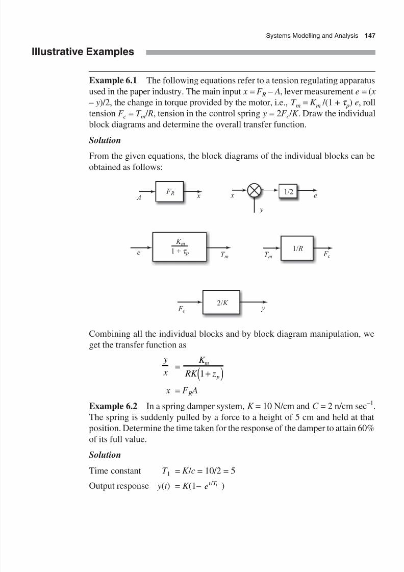
8/11/2019 Introduction to Mechatronics - Appuu Kuttan.pdf
http://slidepdf.com/reader/full/introduction-to-mechatronics-appuu-kuttanpdf 156/345
Systems Modelling and Analysis 147
Illustrative Examples
Example 6.1 The following equations refer to a tension regulating apparatus
used in the paper industry. The main input x = F R – A, lever measurement e = ( x
– y)/2, the change in torque provided by the motor, i.e., T m = K m /(1 + t p) e, rolltension F c = T m / R, tension in the control spring y = 2F c / K . Draw the individual
block diagrams and determine the overall transfer function.
Solution
From the given equations, the block diagrams of the individual blocks can be
obtained as follows:
F R
A x
1/2 x
y
e
T m1/ R
F c
2/ K y
K m1 + t pe T m
F c
Combining all the individual blocks and by block diagram manipulation, we
get the transfer function as
y
x =
K
RK z
m
p1 + x = F R A
Example 6.2 In a spring damper system, K = 10 N/cm and C = 2 n/cm sec–1.
The spring is suddenly pulled by a force to a height of 5 cm and held at that
position. Determine the time taken for the response of the damper to attain 60%
of its full value.
Solution
Time constant T 1 = K / c = 10/2 = 5
Output response y(t ) = K (1– et T / 1 )

8/11/2019 Introduction to Mechatronics - Appuu Kuttan.pdf
http://slidepdf.com/reader/full/introduction-to-mechatronics-appuu-kuttanpdf 157/345
148 Introduction to Mechatronics
60% of the input amplitude,
y(t ) at 60% = 0.6 ¥ K = 0.6 ¥ 5 = 3 cm
Hence the time required for the response to reach 60% of amplitude is 4.58
seconds.
Example 6.3 A servo system for the position control of a rotary table mass is
stabilized by viscous friction damping, which is 75% of that needed for critical
damping. The undamped natural frequency of the system is 16 Hz. Determine
the damped natural frequency and maximum overshoot.
Solution
Since the damping coefficient is 0.75 times the critical damping, the damping
ratio x = 0.75. Therefore, the damped natural frequency
w d = w x n 1 10 582- = .
and the maximum overshoot
M p = e- -Vp V / 1 2
= 2.84%
Example 6.4 Determine the inverse Laplace transform of Y (s), if
Y (s) =– –s s
s s s
2 1
1 2
-
+ +
Solution
The partial fraction expansion of Y (s) is
Y (s) =C
s
C
s
C
s
1 2 3
1 2+
+ +
+ =
1
2
C 1 =
– s s
s sats
2 1
1 20
- -
+ + =
= –1
C 2 =–
–1s s
s sats
2 1
2
- -
+ =
=
–1
2
C 3 =–
–2s s
s sats
2 1
2
- -
+ =
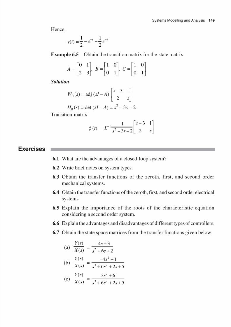
8/11/2019 Introduction to Mechatronics - Appuu Kuttan.pdf
http://slidepdf.com/reader/full/introduction-to-mechatronics-appuu-kuttanpdf 158/345
Systems Modelling and Analysis 149
Hence,
y(t ) =1
2
1
2– –e e
t t - -
Example 6.5 Obtain the transition matrix for the state matrix
A =0 1
2 3
1 0
0 1
1 0
0 1
=
=
, , B C
Solution
W 0 (s) = adj (sI – A)s
s
-
3 1
2
H 0 (s) = det (sI – A) = s2
– 3s – 2
Transition matrix
f (t ) = L–1
1
3 2
3 1
22s s
s
s– –
-
Exercises
6.1 What are the advantages of a closed-loop system?
6.2 Write brief notes on system types.
6.3 Obtain the transfer functions of the zeroth, first, and second order
mechanical systems.
6.4 Obtain the transfer functions of the zeroth, first, and second order electrical
systems.
6.5 Explain the importance of the roots of the characteristic equation
considering a second order system.
6.6 Explain the advantages and disadvantages of different types of controllers.
6.7 Obtain the state space matrices from the transfer functions given below:
(a)Y s
X s
( )
( ) =
–4s
s s
+
+ +
3
6 22
(b)Y s
X s
( )
( ) =
–4s
s s s
2
3 2
1
6 2 5
+
+ + +
(c)Y s
X s
( )
( ) =
3 6
6 2 5
2
3 2
s
s s s
+
+ + +

8/11/2019 Introduction to Mechatronics - Appuu Kuttan.pdf
http://slidepdf.com/reader/full/introduction-to-mechatronics-appuu-kuttanpdf 159/345
150 Introduction to Mechatronics
6.8 Obtain the transfer functions from the state space matrices given below:
(a) A =2 9
1 4-
, B =
4
–3
, C = 2 –6
(b) A =
–6
–9
1 0
0 1
0 0 1
, B =
1
2
1
, C =1 0 0
0 1 0
(c) A =–2
–3
1
0
, B =4
5
, C = 1 0
6.9 Prove the following, if f is the transition matrix:
(a) f (0) = I
(b) f (t 1 + t 2) = f (t 2) f (t 1)
(c) [f (t )]n = f (nt )
6.10 Obtain the computer algorithm for a PI controller.
6.11 Find the Z transform transfer function for the following cases:
(a) y(n + 3) + 3 y(n + 2) – y(n + 1) + y(n) = u(n + 2) + u(n + 1) – 4u(n)
(b) y(n + 3) = 0.5 y(n + 2) – y(n + 1) + 0.125 y(n) = 10 u(n + 3)
(c) y(n + 2) – 5 y(n + 1) – 6 y(n ) = 2u(n)
6.12 Find the inverse Z transform for the following:
(a)Y s
X s
( )
( ) =
4
3 Z +
(b)
Y s
X s
( )
( ) =
z
z2 1–
6.13 Determine whether the discrete systems given below are stable or not.
(a)Y z
U z
( )
( ) =
–3
–
z
z z
2
2
1
4 2 1
++
(b)Y z
U z
( )
( ) =
5 05
2 8 175 0 33 2
( . )
– . . – .
z
z z z
-
+

8/11/2019 Introduction to Mechatronics - Appuu Kuttan.pdf
http://slidepdf.com/reader/full/introduction-to-mechatronics-appuu-kuttanpdf 160/345
Motion Control Devices
Motion control devices are the elements of mechatronic systems, which areresponsible for transforming the output of a microprocessor or control system
into a controlling action on a machine or device. For example, motor control
devices transform electrical signal output from a controller into a linear or rotary
motion. Motion control devices are called servo systems. Hydraulic, pneumatic,
and electrical systems can be used as servo systems. Hydraulic systems are well
suited for large systems in which power requirements are high. The cost of
hydraulic drives is not proportional to the power requirements and, thus, they
are expensive for small- and medium-sized mechatronic systems. However,
the speed of the hydraulic system is very low compared to that of a pneumaticor an electrical system. Pneumatic systems provide fast and high load-carrying
mechatronic systems. The manufacturing of a pneumatic system is expensive,
since the accuracy requirements are high and the working medium is compressed
air. Electrical actuators have a very high speed of operation without any delay.
However, the system is bulky for high-power applications as compared to
hydraulic or pneumatic systems.
A rigid body can have very complex motion, which might seem difficult to describe.
The motion of any rigid body can be considered to be a combination of translationaland rotational motion. By considering three-dimensional (3D) space, a translational
motion can be considered to be the movement that can be resolved into components
along one or more of the three axes of the 3D space. Similarly, rotation can be
considered as a motion that has components rotating about one or more of the axes.
A cyclic motion is a combination of translational and rotational motion. Three axes’
translation and three rotations give six degrees of freedom. If a joint is constrained
to move along a line, then it is a translation with one degree of freedom. A constraint
is needed for each degree of freedom that is to be prevented from occurring, provided
there is no redundant constraint; then the number of the degrees of freedom would

8/11/2019 Introduction to Mechatronics - Appuu Kuttan.pdf
http://slidepdf.com/reader/full/introduction-to-mechatronics-appuu-kuttanpdf 161/345
152 Introduction to Mechatronics
be six minus the number of constraint(s). However, the redundant constraint oftenoccurs. So the basic rule for constraint on a single rigid body is
Number of constraint(s) = Number of degrees of freedom – Number of redundancy
Thus, if a body is required to be fixed, i.e., needs no degree of freedom, no redundant
constraints are introduced and the number of constraints required is 6.
The principle of least constraint(s) is used to design devices. This principle states
that in fixing a body or guiding it to a particular type of motion, the minimum number
of constraints should be used, that is, there should not be redundancy. This is often
referred to as the kinematic design. For example, to have a shaft that rotates only
about one axis with no translation motion, the number of degrees of freedom should
be reduced to 1. Thus, the minimum number of constraints to achieve this is 5 and
any more constraints than this will lead to redundancy. If the shaft is mounted on
one end of a ball bearing and other end is at roller bearing, the bearing pair together
prevents translation and rotation at right angle to the shaft axis. The ball bearingprevents translation along the x axis of the shaft, whereas roller bearing allows
motion along the axis of the shaft. Thus, there is a total of five constraints; which
give one degree of freedom, rotation about axis of the shaft. If there is a ball bearing
at each end of the shaft, then bearings could have prevented translation along the
axis of the shaft, thus, there would have been redundancy. Such redundancy can
cause damage. If ball bearings are used at both ends of the shaft, then in order to
prevent redundancy, one of the bearing’s outer race is not fixed in its housing so that
it could slide in the axial direction.
Actuators are structures that transmit and support load. A joint is a connection
between two or more links at their nodes and allows some motion between the
connected links. Levers, cranks, connecting rods, pistons, sliders, pulleys, belts, and
shafts are all examples of links. A sequence of joints and links is known as a kinematics
chain. For a kinematics chain to transmit motion, one link must be fixed. The
movement of one link produces predictable relative movement of other links in the
chain. For mechatronics system actuation, one can use hydraulic, pneumatic, or
electrical drives with kinematic chains.
7.1 Hydraulic and Pneumatic Actuators
The hydraulic actuation is powered by fluids. Fluids usually are pressurized oils. The
operation of hydraulic actuators is generally similar, except in their ability to contain
the pressure of the fluid. Hydraulic systems operate in a pressure range between
60 bars and 200 bars. The main constituents of a hydraulic system are the power
supply unit, hydraulic fluid, direction control valve, linear and rotary actuators, and
interaction components. The power supply unit is the most important component in
a hydraulic pump. The pump drives the hydraulic fluid from a reservoir (tank) and
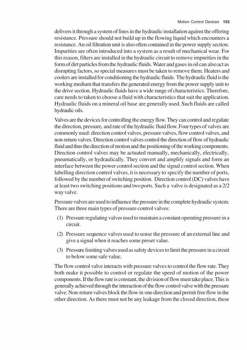
8/11/2019 Introduction to Mechatronics - Appuu Kuttan.pdf
http://slidepdf.com/reader/full/introduction-to-mechatronics-appuu-kuttanpdf 162/345
Motion Control Devices 153
delivers it through a system of lines in the hydraulic installation against the offering
resistance. Pressure should not build up in the flowing liquid which encounters a
resistance. An oil filtration unit is also often contained in the power supply section.
Impurities are often introduced into a system as a result of mechanical wear. For
this reason, filters are installed in the hydraulic circuit to remove impurities in the
form of dirt particles from the hydraulic fluids. Water and gases in oil can also act as
disrupting factors, so special measures must be taken to remove them. Heaters and
coolers are installed for conditioning the hydraulic fluids. The hydraulic fluid is the
working medium that transfers the generated energy from the power supply unit to
the drive section. Hydraulic fluids have a wide range of characteristics. Therefore,
care needs to taken to choose a fluid with characteristics that suit the application.
Hydraulic fluids on a mineral oil base are generally used. Such fluids are called
hydraulic oils.
Valves are the devices for controlling the energy flow. They can control and regulatethe direction, pressure, and rate of the hydraulic fluid flow. Four types of valves are
commonly used: direction control valves, pressure valves, flow control valves, and
non-return valves. Direction control valves control the direction of flow of hydraulic
fluid and thus the direction of motion and the positioning of the working components.
Direction control valves may be actuated manually, mechanically, electrically,
pneumatically, or hydraulically. They convert and amplify signals and form an
interface between the power control section and the signal control section. When
labelling direction control valves, it is necessary to specify the number of ports,
followed by the number of switching position. Direction control (DC) valves have
at least two switching positions and two ports. Such a valve is designated as a 2/2way valve.
Pressure valves are used to influence the pressure in the complete hydraulic system.
There are three main types of pressure control valves:
(1) Pressure regulating valves used to maintain a constant operating pressure in a
circuit.
(2) Pressure sequence valves used to sense the pressure of an external line and
give a signal when it reaches some preset value.
(3) Pressure limiting valves used as safety devices to limit the pressure in a circuit
to below some safe value.
The flow control valve interacts with pressure valves to control the flow rate. They
both make it possible to control or regulate the speed of motion of the power
components. If the flow rate is constant, the division of flow must take place. This is
generally achieved through the interaction of the flow control valve with the pressure
valve. Non-return valves block the flow in one direction and permit free flow in the
other direction. As there must not be any leakage from the closed direction, these

8/11/2019 Introduction to Mechatronics - Appuu Kuttan.pdf
http://slidepdf.com/reader/full/introduction-to-mechatronics-appuu-kuttanpdf 163/345
154 Introduction to Mechatronics
valves always have a poppet design. In the case of a non-return valve, a distinction
is made between ordinary non-return valves and piloted non-return valves. In the
case of piloted non-return valves, flow in the blocked direction can be released by a
signal. Figure 7.1 shows schematic diagrams of various control valves.
(d) 4/2 way valve (e) Adjustable flow valves
(f) 4\3 way valve
Fig. 7.1 Control valves
Cylinders are drive components that convert hydraulic power into mechanical power.
They generate linear movements while passing on the surface of a movable piston.
In single acting cylinders, the fluid pressure can be applied to either side of the
piston, with the result that the drive movement is produced only in one direction. The
return stroke of the piston is affected by an external force or by return speed. In
double acting cylinders, the fluid pressure can be applied to either side of the piston,
with the result that the drive movements are produced in two directions. Like cylinders,
hydraulic motors are drive components controlled by valves. They too convert
hydraulic power into mechanical power, but the difference is that they generate
rotary or swivel movements instead of linear movement. Figure 7.2 shows the
schematic diagrams of a single acting cylinder and a rotary actuator. Two parameters
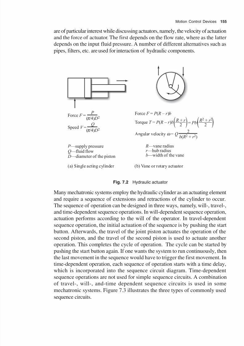
8/11/2019 Introduction to Mechatronics - Appuu Kuttan.pdf
http://slidepdf.com/reader/full/introduction-to-mechatronics-appuu-kuttanpdf 164/345

8/11/2019 Introduction to Mechatronics - Appuu Kuttan.pdf
http://slidepdf.com/reader/full/introduction-to-mechatronics-appuu-kuttanpdf 165/345
156 Introduction to Mechatronics
1.0
1.1
0.1
1.2
(a) Will-dependent circuit
1.0 1.3
1.2
0.1
(b) Travel-dependent circuit
0.3
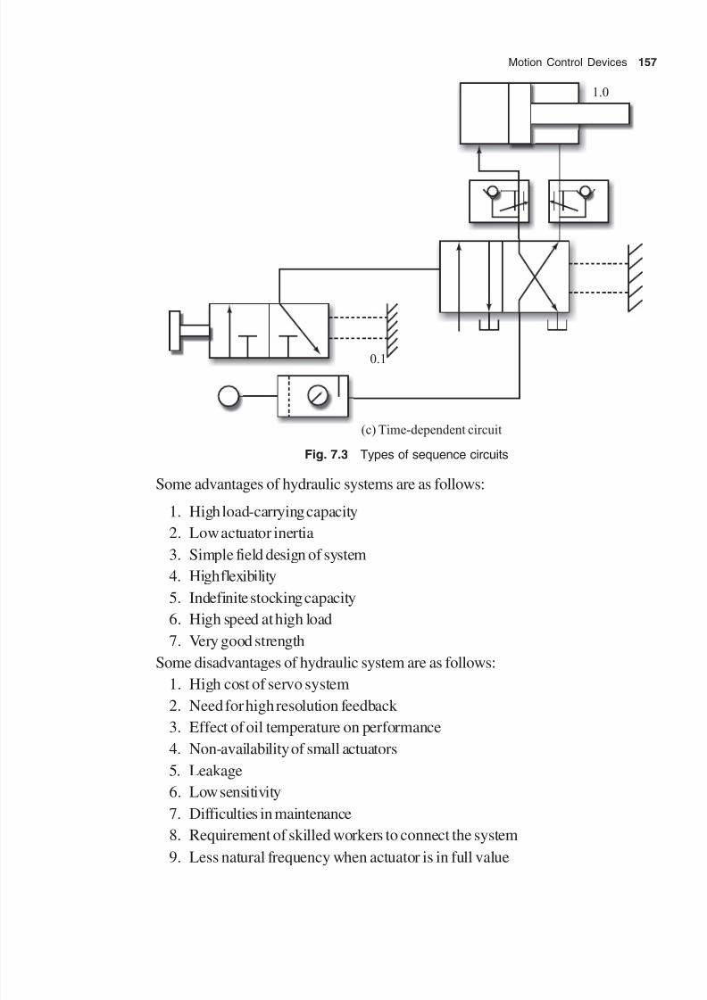
8/11/2019 Introduction to Mechatronics - Appuu Kuttan.pdf
http://slidepdf.com/reader/full/introduction-to-mechatronics-appuu-kuttanpdf 166/345
Motion Control Devices 157
0.1
(c) Time-dependent circuit
1.0
Fig. 7.3 Types of sequence circuits
Some advantages of hydraulic systems are as follows:
1. High load-carrying capacity
2. Low actuator inertia
3. Simple field design of system
4. High flexibility
5. Indefinite stocking capacity
6. High speed at high load
7. Very good strength
Some disadvantages of hydraulic system are as follows:
1. High cost of servo system
2. Need for high resolution feedback
3. Effect of oil temperature on performance
4. Non-availability of small actuators
5. Leakage
6. Low sensitivity
7. Difficulties in maintenance
8. Requirement of skilled workers to connect the system
9. Less natural frequency when actuator is in full value
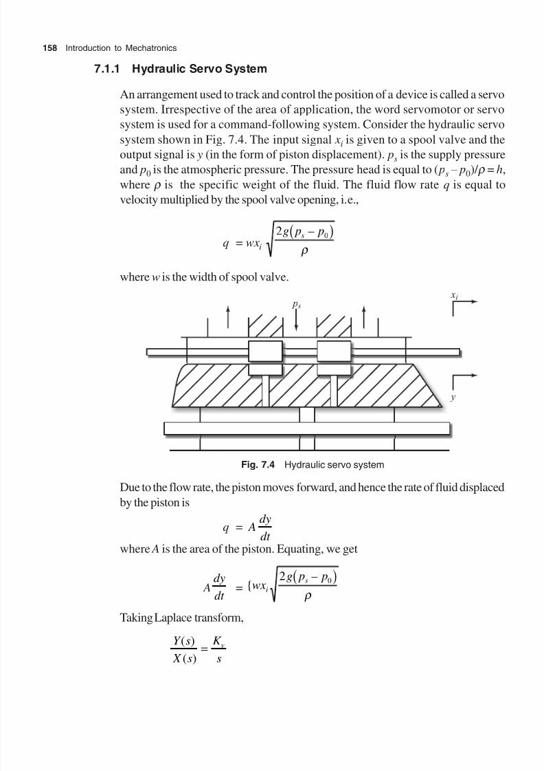
8/11/2019 Introduction to Mechatronics - Appuu Kuttan.pdf
http://slidepdf.com/reader/full/introduction-to-mechatronics-appuu-kuttanpdf 167/345
158 Introduction to Mechatronics
7.1.1 Hydraulic Servo System
An arrangement used to track and control the position of a device is called a servo
system. Irrespective of the area of application, the word servomotor or servo
system is used for a command-following system. Consider the hydraulic servo
system shown in Fig. 7.4. The input signal x i is given to a spool valve and the
output signal is y (in the form of piston displacement). ps is the supply pressure
and p0 is the atmospheric pressure. The pressure head is equal to ( ps – p0)/ r = h,
where r is the specific weight of the fluid. The fluid flow rate q is equal to
velocity multiplied by the spool valve opening, i.e.,
q = wx i
2 0g p ps – r
where w is the width of spool valve.
p s
xi
y
Fig. 7.4 Hydraulic servo system
Due to the flow rate, the piston moves forward, and hence the rate of fluid displaced
by the piston is
q = A dy
dt where A is the area of the piston. Equating, we get
Ady
dt = {
–wx
g p pi
s2 0 r
Taking Laplace transform,
Y s
X s
K
s
v( )
( )=

8/11/2019 Introduction to Mechatronics - Appuu Kuttan.pdf
http://slidepdf.com/reader/full/introduction-to-mechatronics-appuu-kuttanpdf 168/345
Motion Control Devices 159
where K v = W 2 0g p ps – / r A is known as the velocity constant. The hydraulic
servo system acts as an integral system.
7.1.2 Pneumatic System
Pneumatic systems have been used for some considerable time for carrying out
simplest mechanical tasks. In more recent times, such systems have played an
important role in the development of pneumatic technology for automation
through mechatronic systems. A pneumatic system can be broken down into a
number of levels representing hardware and signal flow. Except the energy supply
system, all other levels can be represented as in a hydraulic system. The air
supply for a particular pneumatic application should be sufficient and of adequate
quality. The air is compressed to 1/7th of its volume with the help of an air
compressor and is delivered to an air distribution system in factory. To ensure
proper quality of the air, air service equipment is utilized to prepare the air
before it is applied to a control system. As a rule, all pneumatic components are
designed for a maximum operating pressure of 8–10 bars. But it is recommended
to operate the same between 5 and 6 bars for economic use. An air receiver is
fitted to reduce pressure fluctuations. In normal operations, a compressor is
fitted with the receiver when required, and the receiver is available as a reserve
at all the times. This helps reduce the switching cycle of the compressor. If oil
is required for a pneumatic system, then there should be a separate oil meter
using air service unit. An air service unit is a combination of compressed-air
filter, regulator, and lubricator. The compressed-air filter performs the job of
filtering all contamination from the compressed air flowing through it as well
as water which has already condensed. The purpose of the regulator is to keep
the operating pressure virtually constant regardless of any fluctuation in line
pressure and air consumption. Different types of sequence operations can be
designed using sequence circuits associated with hydraulic systems. Pneumatic
actuators are very useful and have the following advantages:
1. Compressed air is readily available in most factories.2. Compressed air can be stored and conveyed easily to larger distances.
3. Compressed air need not be returned to sump.
4. Compressed air is clean.
5. Operation is fast and offers high load-carrying capacity.
6. Digital and logical switches can be prepared using fluidic circuits.
7. Pneumatic elements are simple and reliable.
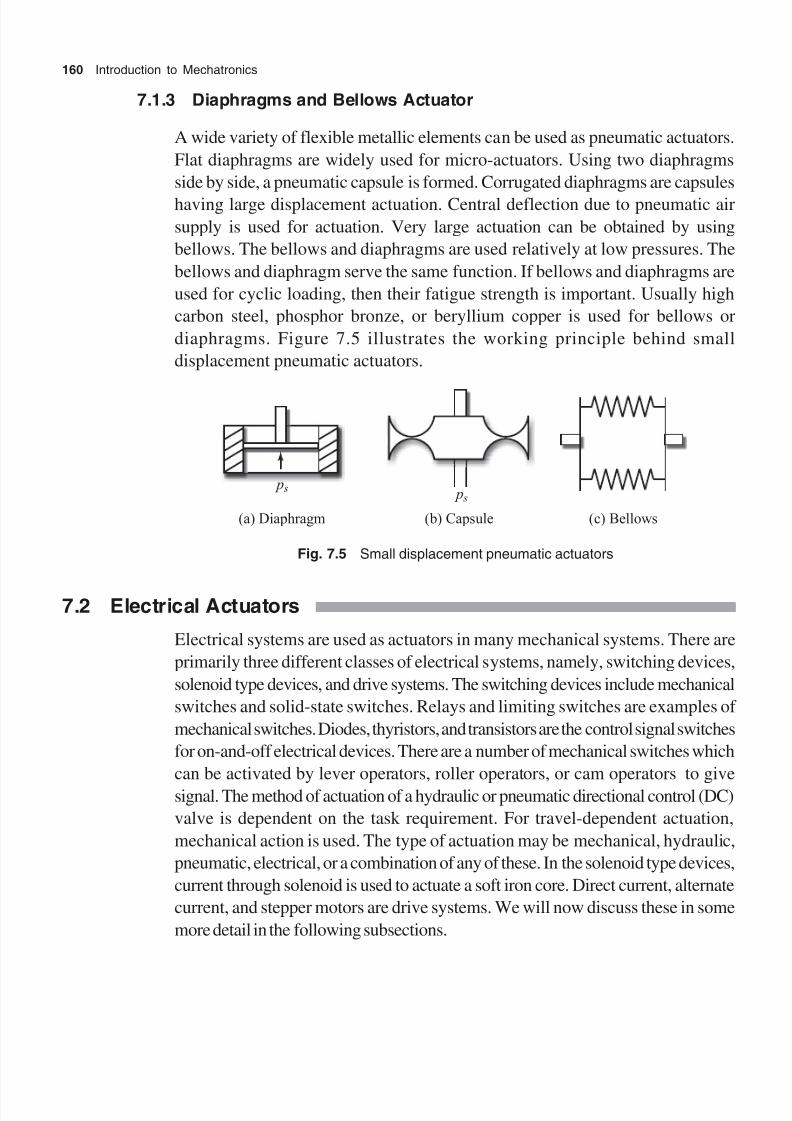
8/11/2019 Introduction to Mechatronics - Appuu Kuttan.pdf
http://slidepdf.com/reader/full/introduction-to-mechatronics-appuu-kuttanpdf 169/345
160 Introduction to Mechatronics
7.1.3 Diaphragms and Bellows Actuator
A wide variety of flexible metallic elements can be used as pneumatic actuators.
Flat diaphragms are widely used for micro-actuators. Using two diaphragms
side by side, a pneumatic capsule is formed. Corrugated diaphragms are capsules
having large displacement actuation. Central deflection due to pneumatic air
supply is used for actuation. Very large actuation can be obtained by using
bellows. The bellows and diaphragms are used relatively at low pressures. The
bellows and diaphragm serve the same function. If bellows and diaphragms are
used for cyclic loading, then their fatigue strength is important. Usually high
carbon steel, phosphor bronze, or beryllium copper is used for bellows or
diaphragms. Figure 7.5 illustrates the working principle behind small
displacement pneumatic actuators.
p s p s
(a) Diaphragm (b) Capsule (c) Bellows
Fig. 7.5 Small displacement pneumatic actuators
7.2 Electrical Actuators
Electrical systems are used as actuators in many mechanical systems. There are
primarily three different classes of electrical systems, namely, switching devices,
solenoid type devices, and drive systems. The switching devices include mechanical
switches and solid-state switches. Relays and limiting switches are examples of
mechanical switches. Diodes, thyristors, and transistors are the control signal switches
for on-and-off electrical devices. There are a number of mechanical switches which
can be activated by lever operators, roller operators, or cam operators to give
signal. The method of actuation of a hydraulic or pneumatic directional control (DC)
valve is dependent on the task requirement. For travel-dependent actuation,
mechanical action is used. The type of actuation may be mechanical, hydraulic,
pneumatic, electrical, or a combination of any of these. In the solenoid type devices,
current through solenoid is used to actuate a soft iron core. Direct current, alternate
current, and stepper motors are drive systems. We will now discuss these in some
more detail in the following subsections.

8/11/2019 Introduction to Mechatronics - Appuu Kuttan.pdf
http://slidepdf.com/reader/full/introduction-to-mechatronics-appuu-kuttanpdf 170/345
Motion Control Devices 161
7.2.1 Mechanical Switches
The electrical relay is an example of the mechanical switch which is used in a
control system as an actuator. It offers a simple on/off switching action in response
to a control signal. Figure 7.6(a) illustrates the mechanics behind the working of a
relay. When current flows through the coil of wire, a magnetic field is produced.This magnetic field pulls a movable arm, called the armature, which forces the
contacts to open or close. Usually, there are two sets of contacts, with one being
opened and the other closed by the actuator. This action can then be used to supply
current to a motor or an electric heater in mechanical systems. The relay may be
used to control the action of pneumatic valves, which in turn control the movement
of the piston. Time relays are controlled relays that facilitate a delayed switching
action. The time delay is usually adjustable and can be initiated after current flow
through the relay coil ceases.
(a) Relay switch
Fig. 7.6 Mechanisms of switches
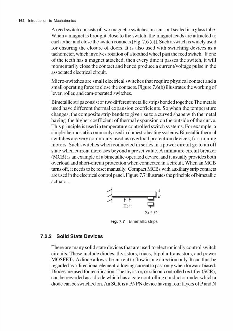
8/11/2019 Introduction to Mechatronics - Appuu Kuttan.pdf
http://slidepdf.com/reader/full/introduction-to-mechatronics-appuu-kuttanpdf 171/345
162 Introduction to Mechatronics
A reed switch consists of two magnetic switches in a cut-out sealed in a glass tube.
When a magnet is brought close to the switch, the magnet leads are attracted to
each other and close the switch contacts [Fig. 7.6 (c)]. Such a switch is widely used
for ensuring the closure of doors. It is also used with switching devices as a
tachometer, which involves rotation of a toothed wheel past the reed switch. If one
of the teeth has a magnet attached, then every time it passes the switch, it will
momentarily close the contact and hence produce a current/voltage pulse in the
associated electrical circuit.
Micro-switches are small electrical switches that require physical contact and a
small operating force to close the contacts. Figure 7.6(b) illustrates the working of
lever, roller, and cam-operated switches.
Bimetallic strips consist of two different metallic strips bonded together. The metals
used have different thermal expansion coefficients. So when the temperature
changes, the composite strip bends to give rise to a curved shape with the metalhaving the higher coefficient of thermal expansion on the outside of the curve.
This principle is used in temperature controlled switch systems. For example, a
simple thermostat is commonly used in domestic heating systems. Bimetallic thermal
switches are very commonly used as overload protection devices, for running
motors. Such switches when connected in series in a power circuit go to an off
state when current increases beyond a preset value. A miniature circuit breaker
(MCB) is an example of a bimetallic-operated device, and it usually provides both
overload and short-circuit protection when connected in a circuit. When an MCB
turns off, it needs to be reset manually. Compact MCBs with auxiliary strip contacts
are used in the electrical control panel. Figure 7.7 illustrates the principle of bimetallicactuator.
Heat
A
B
a a > A B
Fig. 7.7 Bimetallic strips
7.2.2 Solid State Devices
There are many solid state devices that are used to electronically control switch
circuits. These include diodes, thyristors, triacs, bipolar transistors, and powerMOSFETs. A diode allows the current to flow in one direction only. It can thus beregarded as a directional element, allowing current to pass only when forward biased.Diodes are used for rectification. The thyristor, or silicon-controlled rectifier (SCR),can be regarded as a diode which has a gate controlling conductor under which a
diode can be switched on. An SCR is a PNPN device having four layers of P and N

8/11/2019 Introduction to Mechatronics - Appuu Kuttan.pdf
http://slidepdf.com/reader/full/introduction-to-mechatronics-appuu-kuttanpdf 172/345
Motion Control Devices 163
types as shown in Fig. 7.8. There are three terminals, called the anode, cathode, and
gate. The SCR works like a controlled rectifier, in which the conductor can be
controlled by a triggering signal at the gate terminal. The SCR is fixed or turned on
by a pulse of current flowing through its gate. The SCR remains open until it triggers
the gate. Then the SCR latches and remains closed even if the triggering pulse atthe gate is disconnected. The only way to turn off the SCR is by decreasing the
anode current nearly to zero. The triac is similar to the thyristor and is equivalent to
a pair of thyristors connected in reverse and parallel on the same chip. The triac can
be turned on in either the forward or reverse direction. Figure 7.8 illustrates the
basic principle of thyristor and triac, as well as their characteristics.
Fig. 7.8 Thyristor and triac characteristics
Bipolar transistors come in two forms, namely, NPN and PNP forms. For the NPN
transistors, the main current flows in at the collector and out at the emitter. As
against this, the PNP transistor has the main current flowing in at the emitter and
flowing out at the collector. However, the control signal is applied to the base in both
the types. When a small NPN transistor is combined with a large PNP transistor,
the resultant is a large NPN transistor with a large amplification factor. Similarly, a
small PNP transistor in conjunction with a large NPN transistor results in a single,
large PNP transistor. Such a combination of transistors that enables a high current
to be switched with a small input current is termed as a Darlington pair . These

8/11/2019 Introduction to Mechatronics - Appuu Kuttan.pdf
http://slidepdf.com/reader/full/introduction-to-mechatronics-appuu-kuttanpdf 173/345
164 Introduction to Mechatronics
switches are available as a single chip. Bipolar transistor switching is implemented
by basic current. Bipolar transistors allow a higher frequency of switching than
what is possible with a thyristor. However, the power handling capability of bipolar
transistors is less than that of thyristors.
Metal oxide field effect transistors (MOSFETs) come in two types, namely, N-channel and P-channel. The main difference between the use of a MOSFET and a
bipolar transistor for switching is that in MOSFET no current flows into the gate to
exercise control. The gate voltage is the controlling signal, thus the drive circuit can
be amplified in that there is no need to be concerned about the size of the current.
With MOSFETs, very high frequency switching is possible, up to 1 MHz, and interfaces
with a microprocessor are simpler than with bipolar transistors.
7.2.3 Solenoids
Solenoid is a simple and cheap device used to provide electrically operated actuators.
Solenoid valves are an example of devices used to control fluid flow in hydraulic or
pneumatic systems. When current passes through a coil of soft iron, the core is pulled
into the coil, and in doing so, it can open or close parts to allow or stop the flow of fluid.
Two-step control action solenoids are also in use.
7.2.4 Electric Motors
Electric motors are frequently used as fine control unit positional or speed controlsystems. The basic principle governing the operation of a motor is the elctro-
dynamic principle, which states that force is exerted on a conductor when it is
placed in a magnetic field and current passes through it. Force F = BLNI , where
B is the flux density of the magnetic field, L is the length of the conductor, N is
the number of turns, and I is the current flowing through the conductor. Since
the force developed is proportional to the current, thick wires have to be used
for high power electric motors. The second law of electrodynamics states that
when a conductor moves in a magnetic field, an emf, which is equal to the rate
at which the magnetic flux shifts through by the conductor changes, is induced.The induced emf e = BLNV , where V is the velocity at which the conductor is
moving. The second law of electrodynamic is used in electric generators.
The advantages and disadvantages of electric motors are as follows.
Advantages
1. High performance control can be achieved at lower cost.
2. A wide range of motor sizes and capacity is available.

8/11/2019 Introduction to Mechatronics - Appuu Kuttan.pdf
http://slidepdf.com/reader/full/introduction-to-mechatronics-appuu-kuttanpdf 174/345
Motion Control Devices 165
3. Accuracy and repeatability of electric drives are excellent.
4. Electric motors can provide the best resolution.
5. Electric actuators are smaller, hence require less floor space.
6. Temperature stability for overload up to twice of the minimal load for smalldurations is possible.
Disadvantages
1. Limited choice of gear box.
2. Power not as much as provided by a hydraulic system.
3. Need for energy peak loading duty cycle to avoid thermal load on the motor.
4. Motor and gear box inertia is high.
5. To reverse, a special controlled circuit is required.
Motors are classified into two main categories, namely, direct current (DC) and
alternating current (AC) motors. DC motors are used in most of the modern control
systems which act as closed-loop systems. Stepper motors are used for many
mechatronic systems which work as open-loop systems.
In the conventional DC motor, coils of wire are mounted in slots on a cylinder of
magnetic material called armature. The armature is mounted on a bearing and isfree to rotate. It is mounted in the magnetic field produced by field poles. The
magnetic field may be produced by a permanent magnet or an electromagnet.
The field may be self-excited or separately excited. Each end of the armature coil
is connected to the adjacent segments of a segmented ring called commutator.
Electric contacts to the segments are made through the carbon contact called
brushes. As the armature rotates, the commutator reverses the current in each
coil. As it moves between field poles, the direction of rotation of the DC motor
can be reversed by reversing either the armature current or the field current. In
the permanent magnet DC motors, the permanent magnet gives a constant valueof magnetic flux density. The torque developed T = K t I , where K t is known as the
torque constant and is equal to BLN . Since the armature coil is rotating in the
magnetic field, electromagnetic induction occurs and back emf is induced. The
back emf V B = K Bw , where K B is the back emf constant and w is the angular
velocity. Hence, the net voltage acting in the armature winding is V – V B, where V
is the applied voltage. Hence, current in the armature is equal to (V – V B)/ R and
torque T = K t (V – V B)/ R. The construction features and torque–speed characteristic
of a four-pole DC motor are shown in Fig. 7.9.

8/11/2019 Introduction to Mechatronics - Appuu Kuttan.pdf
http://slidepdf.com/reader/full/introduction-to-mechatronics-appuu-kuttanpdf 175/345
166 Introduction to Mechatronics
Stator
Armature
Torque
(a) Construction features (b) Torque–speed characteristic
Speed
Fig. 7.9 DC motor
DC motors with field coil excitation are classified as series, shunt, compound, or
separately excited according to how the field winding and armature winding are
connected. The series wound DC motor exerts the highest starting torque and has
the greatest no-load speed. Reversing the polarity of the supply to the coil has no
effect on the direction of rotation of the motor. With high loads, there is a danger that
the series wound motor runs at a high speed. The shunt wound motor is good for
speed regulation. Because of their constant speed regardless of the load, shunt
wound motors are used widely. Separately excited motors have separate controls
for the armature and field current. For the field-coil DC motor, speed can be changedby varying either the armature current or the field current. Generally, the armature
current is varied. Thus, speed control can be obtained by controlling the applied
voltage to the armature. With an alternating current supply, the thyristor circuit can
be used to control the average voltage applied to the armature.
7.3 DC Servomotor
In servo applications a DC motor is required to reduce rapid acceleration from
standstill. The physical requirements of such a motor are low inertia and highstarting torque. Low inertia is attained with a reduced armature diameter, with
a consequent increase in the armature length such that the desired power output
is achieved. The symbolic representation of an armature controlled DC motor
is shown in Fig. 7.10. In this set-up, an electrical DC source supplies a constant
current I f to the field winding. The armature circuit consists of an armature
resistance Ra and armature inductance La, both are due to the total armature
winding. V is the applied armature voltage and V B is the back emf on the
mechanical side, i.e., the motor rotor. The attached load can be treated as inertia I
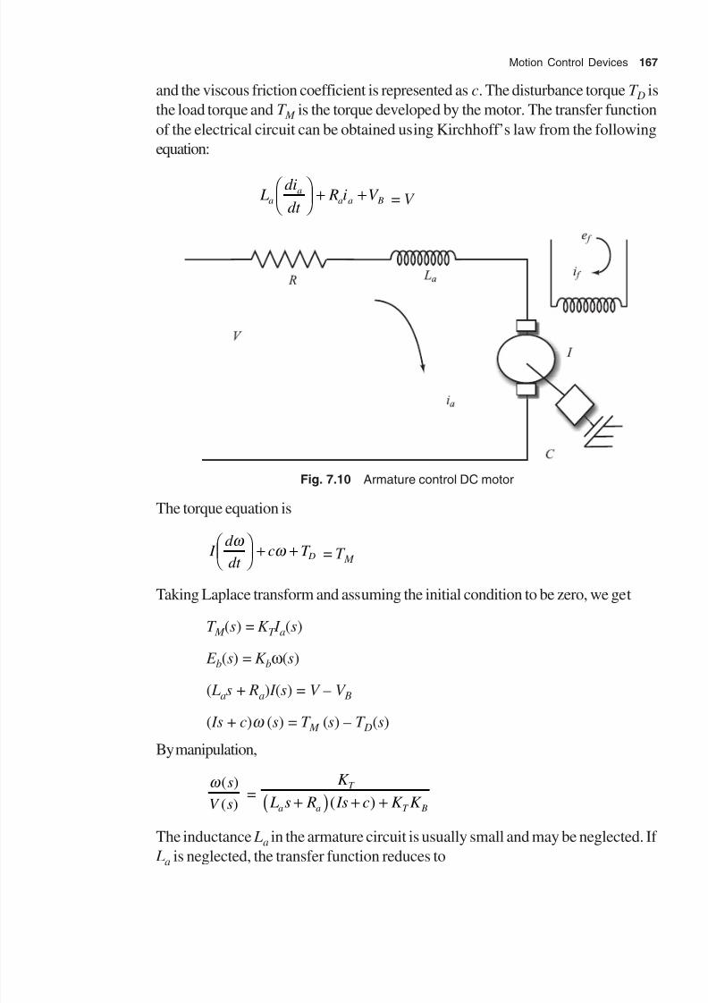
8/11/2019 Introduction to Mechatronics - Appuu Kuttan.pdf
http://slidepdf.com/reader/full/introduction-to-mechatronics-appuu-kuttanpdf 176/345
Motion Control Devices 167
and the viscous friction coefficient is represented as c. The disturbance torque T D is
the load torque and T M is the torque developed by the motor. The transfer function
of the electrical circuit can be obtained using Kirchhoff’s law from the following
equation:
L di
dt R i V a
aa a B
+ + = V
Fig. 7.10 Armature control DC motor
The torque equation is
I d
dt c T D
w w
+ + = T M
Taking Laplace transform and assuming the initial condition to be zero, we get
T M (s) = K T I a(s)
E b(s) = K bw (s)
( Las + Ra) I (s) = V – V B
( Is + c)w (s) = T M (s) – T D(s)
By manipulation,
w ( )
( )
s
V s =
K
L s R Is c K K
T
a a T B+ + + ( )
The inductance La in the armature circuit is usually small and may be neglected. If
La is neglected, the transfer function reduces to

8/11/2019 Introduction to Mechatronics - Appuu Kuttan.pdf
http://slidepdf.com/reader/full/introduction-to-mechatronics-appuu-kuttanpdf 177/345

8/11/2019 Introduction to Mechatronics - Appuu Kuttan.pdf
http://slidepdf.com/reader/full/introduction-to-mechatronics-appuu-kuttanpdf 178/345
Motion Control Devices 169
Its demerits are as follows:
1. Stable control is difficult.
2. Cogging effect—when each slot of the armature comes close to the magnetic
field, there will be stalling.
Pan-cake DC motors provide less cogging effect since the armature
manufacturing adopts the printed circuit board manufacturing technology. It hasa very low inductance capacity compared to the conventional DC motor.
If one needs to use the DC motor as a servo mechanism, a DC motor tachofeedback can be used. The tachogenerator generates a voltage V f proportional tothe actual motor speed but in the opposite polarity. A schematic diagram of the DCservomotor and tachogenerator is shown in Fig. 7.11. Voltage coming in between
the armature is V a = V – V f , where V a is the voltage across the armature and V is thesupply voltage. When the motor is not rotating, V a = V . If V f > V a, the supply voltage
becomes negative. Hence, the motor reduces its speed. Similarly, if the actualspeed of the motor reduces below the set value, then V f is lesser than V a in magnitude.Then the difference is a positive voltage. The positive voltage when applied to thearmature increases the actual speed. This process continues and the speed is regulated
within the band. If the parameter of the system is optimized properly, it is possible toreduce the differential to the minimum so that the set speed is maintained irrespectiveof the load condition.
V
V V V a f = – Motor
V a
V f
Tachogenerator
Fig. 7.11 Servo mechanism for constant speed
7.4 Brushless Permanent Magnet DC Motor
A problem with the DC motor is that it requires a commutator and brushes to
periodically reverse the current through the each armature coil. The brushes
make sliding contact with the commutator and, as a consequence, sparks jump
between the two and the brushes suffer wear. The brushes thus have to be periodically
changed and the commutator requires resurfacing. To avoid this problem, brushless
motors have been designed.

8/11/2019 Introduction to Mechatronics - Appuu Kuttan.pdf
http://slidepdf.com/reader/full/introduction-to-mechatronics-appuu-kuttanpdf 179/345
170 Introduction to Mechatronics
Essentially, a brushless motor consists of a sequence of stator coils and a permanent
magnet rotor. The current carrying conductor in a magnetic field experiences a
force. As a consequence of the reaction force, the magnet will also experience an
opposite and equal force. In the case of the brushless DC motor, the carrying
conductors are fixed and the magnet moves. The rotor is a ferrite or ceramic
permanent magnet. The current to the stator coil is electrically switched by transistors
in sequence around the coils. The switch is controlled by the position of the rotor so
that force is always acting on the magnet, causing it to rotate in the same direction.
Hall sensors are used to sense the position of the rotor and initiate switching by
transistors. The sensors are positioned around the stator.
Brushless permanent magnet DC motors are used in situations where high
performance coupled with reliability and low maintenance is essential. Brushless
permanent magnet DC motors are quiet and capable of high speeds.
7.5 AC Servomotor
The alternating current (AC) motors can be classified into two groups: single
phase and polyphase. Each group is further subdivided into inductive and
synchronous motors. The single-phase induction motor consists of a squirrel cage
rotor in which alluminium or copper bars fit into slots to form electrical circuit.
There is no external connection to the rotor. The stator has a set of windings.
When alternating current passes through the stator, an electromagnetic
induction is induced and the motor rotates. Polyphase (three phase) motor is
similar to the single-phase induction motor but has a stator with three windingslocated 120° apart, each winding being connected to one of the three lines of
the supply. The synchronous motor has stator similar to induction motor but the
rotor in synchronous motor is a parmanent magnet. Single-phase motors tend to
be used for higher power operations. Induction motors tend to be cheaper than
synchronous motors and are thus used widely.
AC motors have some advantages over DC motors; they are cheaper, more rugged,
reliable, and maintenance free. However, speed control in AC motors is generally
more complex than in DC motors. As a consequence, a speed controlled DC drive
generally works out cheaper than a speed controlled AC motor. The speed controlof AC motors is based on the provision of variable frequency supply because the
speed of such motors is determined by the frequency of the supply. The torque
developed by the AC motor is constant when the ratio of the applied stator voltage
to frequency is constant. There are two methods to maintain a constant torque at
different speeds when the frequency is varied and the voltage applied to the stator
also varies. In the first method the AC is first rectified to give a DC with the help
of a converter and then inverted back to AC again, but with a frequency that can be
selected. Another method is often used for operating slow speed and uses the cycle

8/11/2019 Introduction to Mechatronics - Appuu Kuttan.pdf
http://slidepdf.com/reader/full/introduction-to-mechatronics-appuu-kuttanpdf 180/345
Motion Control Devices 171
converter. This converts AC at one frequency directly to AC at another frequencywithout the intermediate DC conversion.
The characteristic features of AC servomotors are as follows:
1. High power density with low weight
2. Low rotor inertia
3. Constant continuous torque and constant overload capacity over the full speedrange
4. No need of additional cooling of the motor
7.6 Stepper Motor
The stepper motor is a device that produces rotation through equal angles, also
called steps, for each digital pulse supplied to it as input. If with such a motor one
pulse produces rotation through 9 deg, then 60 pulses will produce a rotation through
360 deg. There are two types of pulses that are used as the input: unipolar and
bipolar pulses. Figure 7.12(a) shows the difference between unipolar and bipolar
pulses.
N
N
S
S
Stepper motor
(c) Permanent magnet
Unipolar
Bipolar
(a) Pulses motor
S
S
N
N
(b)Variable reluctance stepper
Fig. 7.12 Stepper motor

8/11/2019 Introduction to Mechatronics - Appuu Kuttan.pdf
http://slidepdf.com/reader/full/introduction-to-mechatronics-appuu-kuttanpdf 181/345
172 Introduction to Mechatronics
There are a number of forms of stepper motors. The most commonly used form is
the variable reluctant stepper motor. In this type of the stepper motor the rotor is
made of soft steel. It is cylindrical with four poles. A cylindrical state has few poles
more than the stator. When an opposite pair of windings have current flowing through
them, a magnetic field is produced with lines of force which pass from the statorpoles through the nearest set of poles on the rotor. These lines of force can be
considered to be like elastic threads and are always trying to shorten themselves.
Hence, the rotor will move until the rotor and stator poles line up. This state is
termed the position of minimum reluctance. This form of stepper motor generally
gives a step angle of 7.5 or 15 deg. Figure 7.12(b) shows the schematic diagram of
the variable reluctance stepper motor.
The permanent magnet stepper motor has a stator with poles. Each pole is wound
with field windings, with the coil of opposite pairs of poles being in series. Current is
supplied from a DC source as a pulse train. The rotor is a permanent magnet and
when a pair of stator poles has current switched on, the rotor will move to line up
with it. Thus, for the given current, the rotor moves to the first 45 deg position, and
when polarities are reversed, the rotor will move further 45 deg in order to line up
again . This type of the stepper motor gives step angles of 1.8 deg, 7.5 deg, 15 deg,
30 deg, 34 deg, or 90 deg. Figure 7.12(c) illustrates the working of a permanent
magnet stepper motor.
The hybrid stepper motor combines the features of both the variable reluctance and
permanent magnet motors. It has a permanent magnet encased in iron caps, which
are cut to have teeth. The rotor sets itself in the minimum reluctance position in
response to a pair of stator coils being energized. The typical step angles are 0.9
deg and 1.8 deg. Such stepper motors are extensively used in high-accuracy
positioning applications, for example, in computer hard disk drives.
7.7 Microctuators
The devices used for actuation at micro or mesa scales are called micro actuators.
A microactuator can deliver a desired motion when driven by a power source. Fourprincipal means are commonly used for actuating micro-devices:
1. thermal force,
2. shape memory alloy,
3. piezoelectric crystals, and
4. electrostatic forces.

8/11/2019 Introduction to Mechatronics - Appuu Kuttan.pdf
http://slidepdf.com/reader/full/introduction-to-mechatronics-appuu-kuttanpdf 182/345
Motion Control Devices 173
Electromagnetic actuators are widely used in devices at macro scales. However,
these are rarely used in micro-devices because of the lack of the sufficient space in
micro-devices to accommodate a coil inductance for generating sufficient magnetic
field for actuation power. The obvious weakness of the electrostatic actuator is the
inherent low magnitude. However, not much force is required to actuate mostmicro devices; instead electrostatic actuation is used.
Bimetallic strips are actuators based on the phenomenon that forces a strip to bend
when it is heated or cooled from some initial reference temperature. The bimetallic
strip principle has been used to produce several micro actuators such as micro-
clamps or valves.
Shape memory alloys (SMAs) can produce microactuators more accurately and
effectively. Nitinol or TiNi alloys act as shape memory alloys. These alloys tend to
return to their original shape at a preset temperature. Figure 7.13 illustrates the
working principle of a microactuator using SMA. An SMA strip is originally in a
bent shape at a designed preset temperature. The strip is set straight at room
temperature. However, heating a beam with the attached SMA strip promotes the
strip memory to return to its original bent shape. The deformation of the SMA strip
causes the attached section of the beam to deform, thus causing microactuation of
the beam.
Constraint beam
SMA
Resistance heating
Fig. 7.13 Microactuation using SMA
Certain crystals such as quartz deform with the application of electric voltage. Thisphenomenon is known as piezoelectric actuation. Piezoelectric actuation is used in
micro-positioning mechanisms and micro-clamps. Piezocrystals with electrodes can
be mounted on a silicon cantilever beam for microactuation.
Electrostatic forces are used as driving forces for many actuators. Accurate
assessment of electrostatic forces is an essential part of the design of many micro-
motors and actuators. Figure 7.14 represents two charged plates separated by a
dielectric material with a gap d . The plates become electrically charged when an

8/11/2019 Introduction to Mechatronics - Appuu Kuttan.pdf
http://slidepdf.com/reader/full/introduction-to-mechatronics-appuu-kuttanpdf 183/345
174 Introduction to Mechatronics
electromotive force or voltage is applied to them. This induces capacitance in the
charged plates. The induced capacitance in the charged plates can be expressed as
C =e e r WL
d
0
where W is the width of the plate, L is the length of the plate, e r is the relative
permeability, e 0 is the permeability of air, and d is the distance between the plates.
The energy associated with the electric potential can be expressed as
U = –1
2CV
2 = e e r
WLV
d 0
2
2
The associated electrostatic force that is normal to the plates in the direction of d is
F d = –
dU
da
WLV
d r =
e e 0
2
2
Similarly, the force along the direction of width F W = e r e 0 LV 2 / d and the force along
the length direction F L = e r e 0WV 2 / d . F W is independent of the width and F L is
independent of the length. These electrostatic forces are prime driving forces of
micromotors.
Fig. 7.14 Electrostatic forces in parallel plates
7.7.1 Microgripper
The electrostatic force generated in parallel charged plates can be used as the
driving force for gripping an object. The required gripping force in a gripper
can be provided by normal forces or by in plane force from a pair of misaligned
plates. The arrangement that uses normal gripping forces from parallel plates
[Fig. 7.15 (a)] appears to be simple in practice. The major disadvantage of this
arrangement is that excessive space is required for occupying the electrode in the
microgripper. Consequently, it is rarely used. The other arrangement, shown in
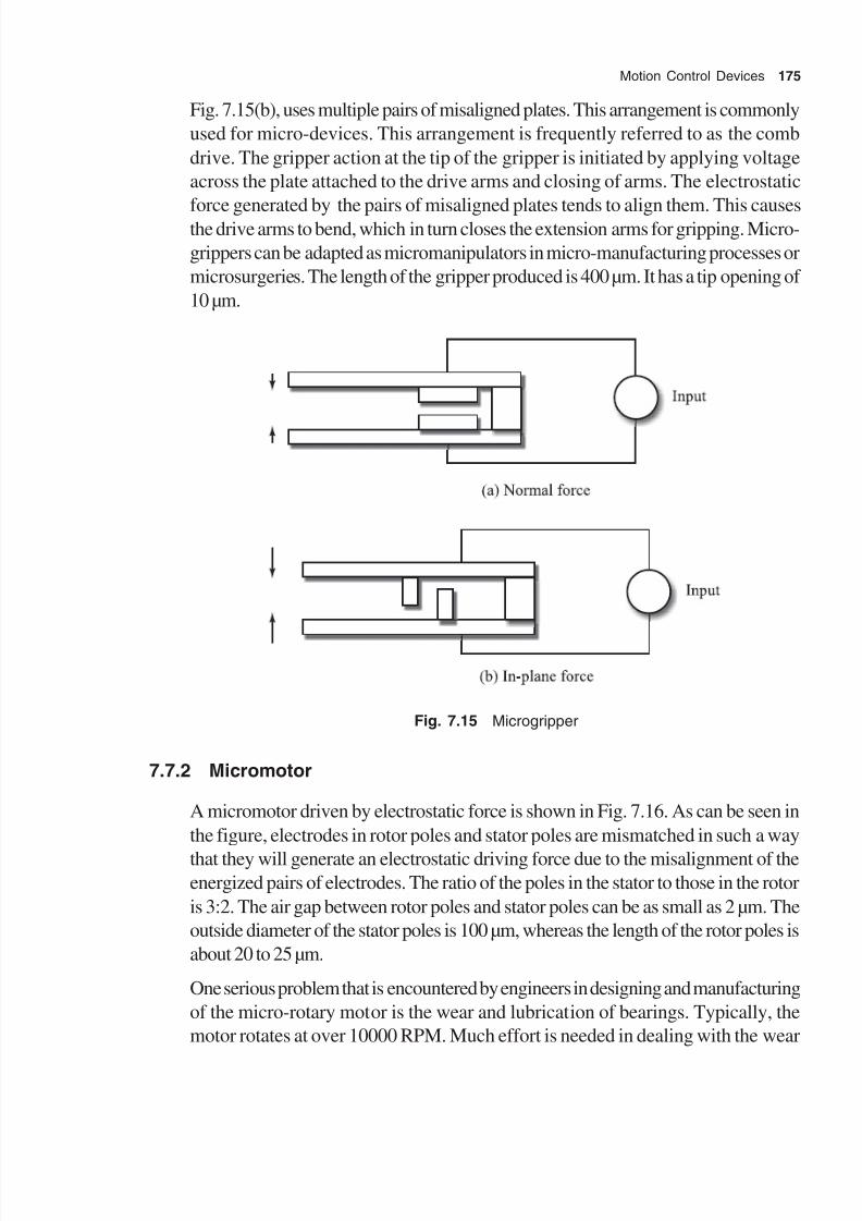
8/11/2019 Introduction to Mechatronics - Appuu Kuttan.pdf
http://slidepdf.com/reader/full/introduction-to-mechatronics-appuu-kuttanpdf 184/345
Motion Control Devices 175
Fig. 7.15(b), uses multiple pairs of misaligned plates. This arrangement is commonly
used for micro-devices. This arrangement is frequently referred to as the comb
drive. The gripper action at the tip of the gripper is initiated by applying voltage
across the plate attached to the drive arms and closing of arms. The electrostatic
force generated by the pairs of misaligned plates tends to align them. This causesthe drive arms to bend, which in turn closes the extension arms for gripping. Micro-
grippers can be adapted as micromanipulators in micro-manufacturing processes or
microsurgeries. The length of the gripper produced is 400 µm. It has a tip opening of
10 µm.
Fig. 7.15 Microgripper
7.7.2 Micromotor
A micromotor driven by electrostatic force is shown in Fig. 7.16. As can be seen in
the figure, electrodes in rotor poles and stator poles are mismatched in such a way
that they will generate an electrostatic driving force due to the misalignment of theenergized pairs of electrodes. The ratio of the poles in the stator to those in the rotor
is 3:2. The air gap between rotor poles and stator poles can be as small as 2 µm. The
outside diameter of the stator poles is 100 µm, whereas the length of the rotor poles is
about 20 to 25 µm.
One serious problem that is encountered by engineers in designing and manufacturing
of the micro-rotary motor is the wear and lubrication of bearings. Typically, the
motor rotates at over 10000 RPM. Much effort is needed in dealing with the wear
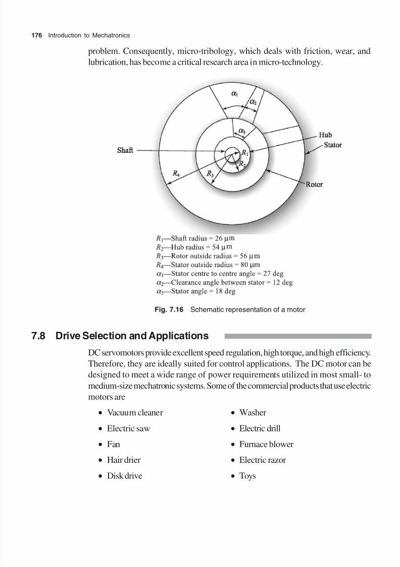
8/11/2019 Introduction to Mechatronics - Appuu Kuttan.pdf
http://slidepdf.com/reader/full/introduction-to-mechatronics-appuu-kuttanpdf 185/345
176 Introduction to Mechatronics
problem. Consequently, micro-tribology, which deals with friction, wear, and
lubrication, has become a critical research area in micro-technology.
Fig. 7.16 Schematic representation of a motor
7.8 Drive Selection and Applications
DC servomotors provide excellent speed regulation, high torque, and high efficiency.
Therefore, they are ideally suited for control applications. The DC motor can be
designed to meet a wide range of power requirements utilized in most small- to
medium-size mechatronic systems. Some of the commercial products that use electric
motors are
∑ Vacuum cleaner ∑ Washer
∑ Electric saw ∑ Electric drill
∑ Fan ∑ Furnace blower
∑ Hair drier ∑ Electric razor
∑ Disk drive ∑ Toys

8/11/2019 Introduction to Mechatronics - Appuu Kuttan.pdf
http://slidepdf.com/reader/full/introduction-to-mechatronics-appuu-kuttanpdf 186/345
Motion Control Devices 177
Stepper motors are not appropriate drives for heavy-duty mechatronic systems.
The allowable speed of a stepper motor is a function of its load torque. But load
torque strongly depends on the system load required. An excessive load on the
stepper motor might cause a subsequent loss of steps. In addition, stepper motors
are limited in resolution and tend to be noisy. For all of these reasons, steppermotors are seldom used in mechatronic systems which require a high torque. Stepper
motors are very popular due to their functional capabilities such as the following:
1. Precision incremental movements in steps.
2. Repeatability and precision in positioning.
3. Reliable design, since brush, gear box, etc. are not needed.
The disadvantage of the stepper motor is that resonance can occur at high speeds.
The applications of stepper motor are found in dot matrix printers, open-loopNC equipment, scanners, disk drives, machine tools, XY recorders, and robotics.
Hydraulic or pneumatic devices are well suited for large mechatronic systems where
power requirements are high. The cost of the hydraulic drive is not proportional to
the power required, and thus is expensive for small- and medium-size mechatronic
systems. Some of the applications of hydraulic or pneumatic systems are in robotics,
earth excavators, automatic mine diggers, etc.
Presently microactuators are widely used in many applications, which include the
following:
1. Nanometrology
2. Optical device alignment
3. Micro-fan and micro-pump
4. Autofocusing system
5. Dick spin stand
6. Bio-mimetic robot
7. Micro-lithography
8. CD-ROM lead contact
9. Nano-positioning
Figure 7.17 gives some qualitative rather than quantitative selection guidelines for
choosing actuators.

8/11/2019 Introduction to Mechatronics - Appuu Kuttan.pdf
http://slidepdf.com/reader/full/introduction-to-mechatronics-appuu-kuttanpdf 187/345
178 Introduction to Mechatronics
Hydraulic
Paneumatic
DC motor
Stepper motor
Volume
AC
(a) Torque versus volume of actuators
Electrical
Hydraulic
Power
(b) Weight versus power of the electrical and hydraulic actuators
Electrical
Hydraulic
Power
(c) Cost versus power of the electrical and hydraulic actuators
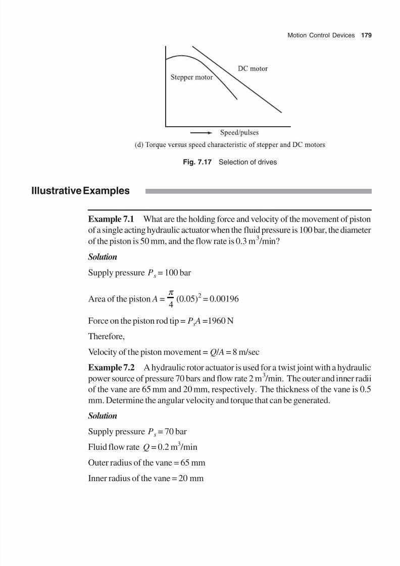
8/11/2019 Introduction to Mechatronics - Appuu Kuttan.pdf
http://slidepdf.com/reader/full/introduction-to-mechatronics-appuu-kuttanpdf 188/345
Motion Control Devices 179
Fig. 7.17 Selection of drives
Illustrative Examples
Example 7.1 What are the holding force and velocity of the movement of piston
of a single acting hydraulic actuator when the fluid pressure is 100 bar, the diameter
of the piston is 50 mm, and the flow rate is 0.3 m3 /min?
Solution
Supply pressure Ps = 100 bar
Area of the piston A =p
4 (0.05)2 = 0.00196
Force on the piston rod tip = Ps A =1960 N
Therefore,
Velocity of the piston movement = Q / A = 8 m/sec
Example 7.2 A hydraulic rotor actuator is used for a twist joint with a hydraulic
power source of pressure 70 bars and flow rate 2 m3 /min. The outer and inner radii
of the vane are 65 mm and 20 mm, respectively. The thickness of the vane is 0.5
mm. Determine the angular velocity and torque that can be generated.
Solution
Supply pressure Ps = 70 bar
Fluid flow rate Q = 0.2 m3 /min
Outer radius of the vane = 65 mm
Inner radius of the vane = 20 mm

8/11/2019 Introduction to Mechatronics - Appuu Kuttan.pdf
http://slidepdf.com/reader/full/introduction-to-mechatronics-appuu-kuttanpdf 189/345
180 Introduction to Mechatronics
Width of the vane = 0.5 mm
Torque developed =1
2
2 2 p b R r s – = 669.37 N-cm
Angular velocity = 22 2
Q R r b–
= 3.29 m/sec
Example 7.3 A motor has torque constant K t = 100 Nm A and voltage constant
of 12 V(/kilo revolution/min). The armature resistance is 2 W. If 24 V voltage is
applied to the terminal, what would be (a) the torque at the rotor (b) speed at
zero load, and (c) torque at 100 revolution/min. Plot the result as a speed versus
torque graph.
Solution
At zero RPM, the back emf developed
V B = 0
The armature current
I = V / Ra = 24/2 = 12
Therefore, generated torque
K t I = 10 ¥ 12 = 120 N-m
At no load, the input voltage is equal to the back emf,
24 = 12 V/(kilo revolution/min) ¥ w
Hence, the angular speed
w = 2 kilo revolution/min = 2000 RPM
120 N
2000
Speed
Fig. 7.18 Speed–torque characteristic

8/11/2019 Introduction to Mechatronics - Appuu Kuttan.pdf
http://slidepdf.com/reader/full/introduction-to-mechatronics-appuu-kuttanpdf 190/345

8/11/2019 Introduction to Mechatronics - Appuu Kuttan.pdf
http://slidepdf.com/reader/full/introduction-to-mechatronics-appuu-kuttanpdf 191/345
182 Introduction to Mechatronics
1.2
1.0
0.1
A B
1.1
P T
Fig. 7.19 Circuit diagram for opening a door in furnace
Example 7.6 A differential cylinder is on one side of the piston area A = 10 cm2
and the annular piston surface area on other side is A p = 5 cm2
. The stroke length sis 10 cm. The pump delivers 10 L/min and the maximum pressure is 100 bar.
Determine the speed of advance (pitch) and return stroke. Determine the time
taken to extend and retract the piston and the maximum force which can be attained
on extending and retracting. Figure 7.20 shows the hydraulic cylinder.
Fig. 7.20 Hydraulic cylinder
Solution
Velocity during advance =Q
A= =
10000
1010m/sec
8/11/2019 Introduction to Mechatronics - Appuu Kuttan.pdf
http://slidepdf.com/reader/full/introduction-to-mechatronics-appuu-kuttanpdf 192/345
Motion Control Devices 183
Velocity during retraction =Q
A p
= =10000
520 m/sec
Time for advance = s / v = 100/1000 = 6 sec
Time for retraction = s / v= 100/1000 = 3 secForce during advance = P ¥ A = 1000 N ¥ 10 = 10000 N
Force during retard = P ¥ AP = 1000 N ¥ 5 = 5000 N
Example 7.7 Calculate normal electrostatic force exerted on a 1 mm ¥ 1 mm
plate of e r =1.0 for air dielectric and e 0 = 8.85 pF/m or 8.85 ¥ 10–12
C2 /N m
2 for
material.
Solution
Width of the plate = 1 mm
Length of the plate = 1 mm
Dielectric constant for air = 1.0
Dielectric constant for material = 8.85 ¥ 10–12
C2 /N-m
2
Normal electrostatic force developed
F d = e r e 0 WLV 2 /2d = –1.106 10–6 V2 N
Thus, 11 mN force is generated for a voltage of 100 V applied to the plate.
Exercises
7.1 What is a servo system? Explain with a suitable sketch the working of a hydraulic
servo system.
7.2 What is the velocity of the piston and the force generated by it if the fluid
pressure is 50 bar inside the cylinder? The piston diameter is 80 mm and flow
rate is 8 cm3 /min.
7.3 A hydraulic rotary servo actuator is to be used for a twist joint with a hydraulic
power system. The outer and the inner radii of the vane are 80 mm and 20
mm, respectively. The width of each vane is 10 mm. Determine the angular
velocity and torque generated if the supply pressure is 50 bar and the flow rate
is 8 cm3 /min.
7.4 List out the symbols of different elements used in hydraulic and pneumatic
systems.

8/11/2019 Introduction to Mechatronics - Appuu Kuttan.pdf
http://slidepdf.com/reader/full/introduction-to-mechatronics-appuu-kuttanpdf 193/345
184 Introduction to Mechatronics
7.5 What are the advantages and disadvantages of a pneumatic power system
and a hydraulic power system?
7.6 Differentiate between thyristor and triac.
7.7 Explain SCR and MCB.
7.8 Obtain the transfer function of a DC motor with load.
7.9 What is a brushless DC motor?
7.10 Sketch and explain the working of an AC servomotor.
7.11 Sketch and explain the working of a magnetic stepper motor.
7.12 What is micro-actuation? Explain the principles used for micro-actuation.
7.13 Sketch and explain the working of a microgripper.
7.14 Explain the principle and working of a micromotor.
8/11/2019 Introduction to Mechatronics - Appuu Kuttan.pdf
http://slidepdf.com/reader/full/introduction-to-mechatronics-appuu-kuttanpdf 194/345
Sensors and Transducers
A transducer is a device, usually electrical, electronic, or electro-mechanical,
that converts one type of energy into another for various purposes including
measurement or information transfer. In a broader sense, a transducer is
sometimes defined as any device that converts a signal from one form into
another. The term ‘sensor’ is often used in place of the transducer. A sensor is
defined as an element which when subjected to some physical change experiences
a relative change. Transducers/sensors may act as passive or active devices. A
sensor in which the output energy is supplied entirely or almost entirely by its
input signals is called a passive element. An active element has an auxiliary
source of power that supplies a major part of the output power. There may or
may not be a conversion of energy from one form to another.
The treatment of the instrument performance characteristics is generally broken
down into two subareas: static characteristics and dynamic characteristics. The
static characteristics are the values given when steady state conditions occur.
The dynamic characteristics refer to the behaviour between the time that the
input value changes and the time required given by a transducer to settle down
to steady state values. Accuracy, precision, threshold, resolution, hystersis, dead
band, sensitivity, non-linearity, range or span, and errors are examples of the
static performance characteristic parameters. The response time, time constant,settling time, peak time, rise time are examples of the dynamic performance
characteristics. For better functioning of mechatronics, sensors or transducers,
both static and dynamic parameters are very important. Sensors or transducers
are used in mechatronics for the following purposes:
1. To provide position, velocity, and acceleration information of the measuring
element in a system which provides feedback information
2. To act as protective mechanism for a system

8/11/2019 Introduction to Mechatronics - Appuu Kuttan.pdf
http://slidepdf.com/reader/full/introduction-to-mechatronics-appuu-kuttanpdf 195/345
186 Introduction to Mechatronics
3. To help eliminate mechanically complex and expensive feeding and sorting
devices
4. To provide identification and indication of the presence of different
components
5. To provide real time information concerning the nature of the task being
performed
8.1 Static Performance Characteristics
This section gives the definitions of the static performance characteristic
parameters (see Fig. 8.1).
Accuracy is defined as the proximity of the measured value to the true value. It
is expressed as a percentage of the full range output or full-scale deflection.Precision or repeatability is used to describe the ability of the instrument to give
the same output for repeated application(s) of the same input value. Accurate
sensors are always precise, but vice versa may not be true.
Sensitivity is defined as the ratio of the incremental change in output to the
incremental change in input. More sensitive the instrument, better the readability.
Threshold is the minimum input signal required by the instrument to start
functioning from its initial position.
Resolution is the smallest increment that can be measured in any range of the
sensor.
Hysteresis A sensor can give different outputs for the same value of quantity
being measured depending on whether that value is reached by a continuously
increasing or decreasing change. This effect is called hysteresis.
Hysteresis error is the maximum difference in the input or output for the
increasing and decreasing input value.
Dead band or dead space of a transducer is the range of the input value forwhich there is no output.
Drift is the change in output that occurs over a time. It may be expressed as a
percentage of the full range output. The term ‘zero drift’ is used for the changes
that occur in the output when there is zero input.
Error is the difference between the actual results of the measurement and the
time value of the quantity being measured. The error may be a systemic error or
random error. Systemic errors may arise due to calibration errors, computing
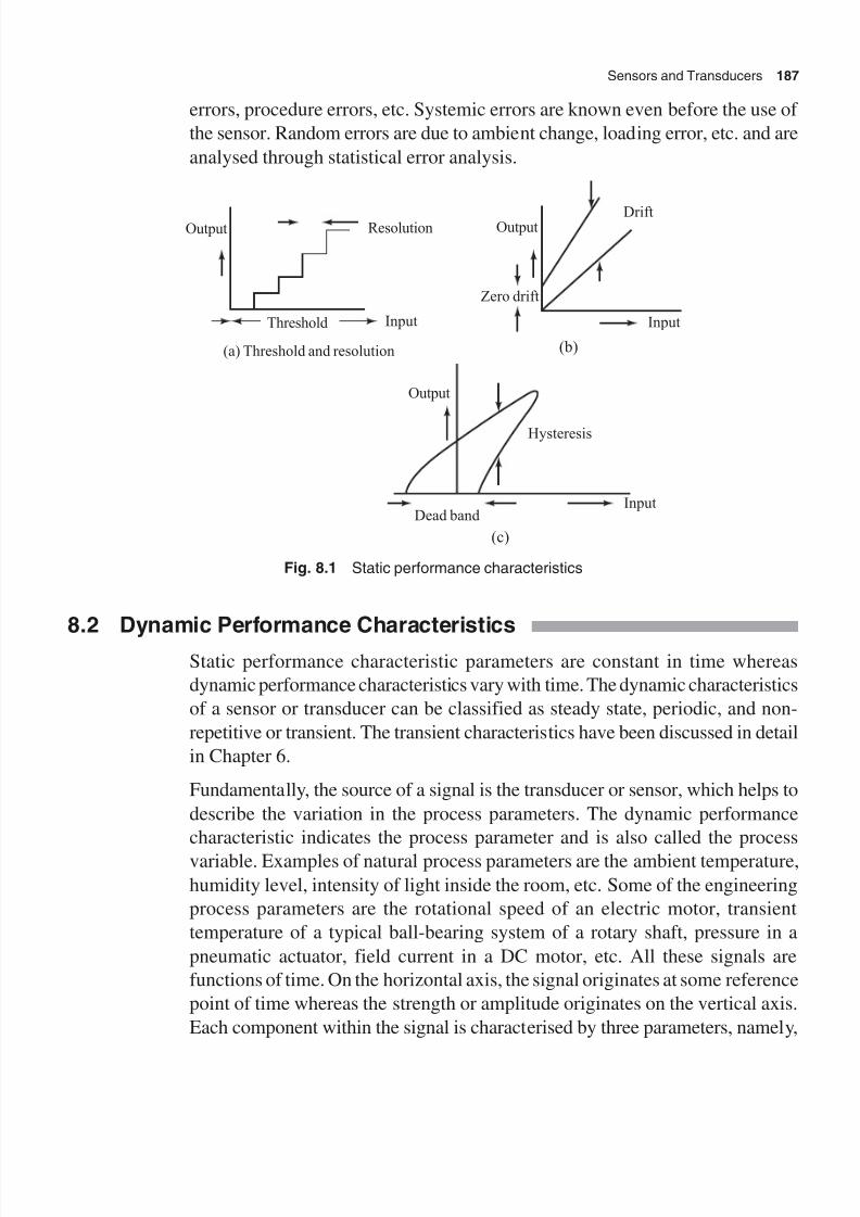
8/11/2019 Introduction to Mechatronics - Appuu Kuttan.pdf
http://slidepdf.com/reader/full/introduction-to-mechatronics-appuu-kuttanpdf 196/345
Sensors and Transducers 187
errors, procedure errors, etc. Systemic errors are known even before the use of
the sensor. Random errors are due to ambient change, loading error, etc. and are
analysed through statistical error analysis.
Output Resolution
InputThreshold
(a) Threshold and resolution
OutputDrift
Zero drift
Input
Output
Hysteresis
Dead band
(b)
(c)
Input
Fig. 8.1 Static performance characteristics
8.2 Dynamic Performance Characteristics
Static performance characteristic parameters are constant in time whereas
dynamic performance characteristics vary with time. The dynamic characteristics
of a sensor or transducer can be classified as steady state, periodic, and non-
repetitive or transient. The transient characteristics have been discussed in detail
in Chapter 6.
Fundamentally, the source of a signal is the transducer or sensor, which helps to
describe the variation in the process parameters. The dynamic performance
characteristic indicates the process parameter and is also called the process
variable. Examples of natural process parameters are the ambient temperature,
humidity level, intensity of light inside the room, etc. Some of the engineering
process parameters are the rotational speed of an electric motor, transient
temperature of a typical ball-bearing system of a rotary shaft, pressure in a
pneumatic actuator, field current in a DC motor, etc. All these signals are
functions of time. On the horizontal axis, the signal originates at some reference
point of time whereas the strength or amplitude originates on the vertical axis.
Each component within the signal is characterised by three parameters, namely,
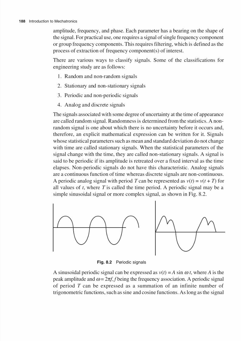
8/11/2019 Introduction to Mechatronics - Appuu Kuttan.pdf
http://slidepdf.com/reader/full/introduction-to-mechatronics-appuu-kuttanpdf 197/345
188 Introduction to Mechatronics
amplitude, frequency, and phase. Each parameter has a bearing on the shape of
the signal. For practical use, one requires a signal of single frequency component
or group frequency components. This requires filtering, which is defined as the
process of extraction of frequency component(s) of interest.
There are various ways to classify signals. Some of the classifications forengineering study are as follows:
1. Random and non-random signals
2. Stationary and non-stationary signals
3. Periodic and non-periodic signals
4. Analog and discrete signals
The signals associated with some degree of uncertainty at the time of appearance
are called random signal. Randomness is determined from the statistics. A non-random signal is one about which there is no uncertainty before it occurs and,
therefore, an explicit mathematical expression can be written for it. Signals
whose statistical parameters such as mean and standard deviation do not change
with time are called stationary signals. When the statistical parameters of the
signal change with the time, they are called non-stationary signals. A signal is
said to be periodic if its amplitude is retreated over a fixed interval as the time
elapses. Non-periodic signals do not have this characteristic. Analog signals
are a continuous function of time whereas discrete signals are non-continuous.
A periodic analog signal with period T can be represented as v(t ) = v(t + T ) forall values of t , where T is called the time period. A periodic signal may be a
simple sinusoidal signal or more complex signal, as shown in Fig. 8.2.
Fig. 8.2 Periodic signals
A sinusoidal periodic signal can be expressed as v(t ) = A sin w t , where A is the
peak amplitude and w = 2p f , f being the frequency association. A periodic signal
of period T can be expressed as a summation of an infinite number of
trigonometric functions, such as sine and cosine functions. As long as the signal

8/11/2019 Introduction to Mechatronics - Appuu Kuttan.pdf
http://slidepdf.com/reader/full/introduction-to-mechatronics-appuu-kuttanpdf 198/345
Sensors and Transducers 189
has a finite number of maxima and minima and is discontinuous within T , the
periodic signal can be expressed as
v(t ) =a
a nf
T b
nf
T n
nn
n
0
1 12
2 2+ +
=
•
=
•
 Âcos sinp p
The above equation is called a Fourier series expansion of f . The component ofthe time periodic signal is called fundamental frequency. a0 is the derivativecomponent of the signal, and an and bn are the coefficients of the trigonometricfunctions. The constants can be obtained by using the following equations:
a0 =2
0
0
T v t dt
t
t T
+
an =2 2
0
0
T
v t nf
T
dt t
t T
cos p +
bn =2 2
0
0
T v t
nf
T dt
t
t T
sin p +
The frequency counts of any periodic signal can be immediately obtained fromthe time domain equations of the Fourier series. Fourier transform (FT) is amathematical tool that transforms a time domain signal into a frequency domainsignal. A time domain signal can also be extracted from a frequency domain
signal. Mathematically,
FT [v(t )] = v( f ) = v t e dt ft
( )–
–
p
•
+•
L
– 1F (t )v(t ) = v(t ) = v t e dt
ft ( )
–
2p
•
+•
8.3 Internal Sensors
Feedback sensors provided in mechatronic systems are called internal sensors.Internal sensor devices are specifically chosen to suit the need for a particulartask. Internal sensors are needed for the feedback of position, velocity or
acceleration of various elements in the mechantronic systems. Internal sensorsmay be classified as potentiometers, tachometers, resolvers, optical encoders,Hall effect sensors, and Moire’s fringes.
8.3.1 Potentiometer
A potentiometer consists of a resistance element and a wiper. It is provided
with three terminals; one at each end of the resistance element and one for the
wiper. The output signal of the potentiometer is the resistance between one end
of the resistance wire and the wiper terminal. According to the type of resistance

8/11/2019 Introduction to Mechatronics - Appuu Kuttan.pdf
http://slidepdf.com/reader/full/introduction-to-mechatronics-appuu-kuttanpdf 199/345
190 Introduction to Mechatronics
element, potentiometers can be divided into three classes: wire wound, cement,
and plastic potentiometers. The wire wound potentiometer is usually a nichrome
wire made of 75 per cent nickel and 25 per cent chromium. Its resistance is not
more than 0.055 W for a temperature change from 25°C to 125°C. The linearity
of the wire wound potentiometer is within ±0.003 per cent. Cementpotentiometers are usually used in electronic circuits. Plastic potentiometers
are also called conductive plastic potentiometers. Conductive plastics are made
up of epoxy polyester and other resins which are blended with carbon powder
to make them conductive. Linearity can be held at 0.025 per cent. The device
gives one million cycles of operation. Figure 8.3 illustrates the schematic diagram
of a potentiometer and its characteristics.
V 0
R P x
R L V L
R P (1– ) x
Fig. 8.3 Potentiometer with load
The potential difference across the load V L is directly proportional to only theinput voltage V 0 if the load resistance is infinite. For finite loads, the relationship
between the output and slide position is non-linear. The potentiometer resistance
RP(1 – x ) is in parallel with the load resistance R L. The combined resistance is
given by R L xRP /( R L + xRP).
Total resistance = RP(1 – x ) + R x R
R x R
L P
L P+
Hence
V
V
L
0
= xR R R R
R x xR R R xR
x
R
R x x
L P L P
P L P L P P
L
/ ( )
( ) / ( )( )
+
- + +=
- +1
1 1
If the load is of infinite resistance, then V L = V 0. Hence, the error due to load
having finite resistance is equal to
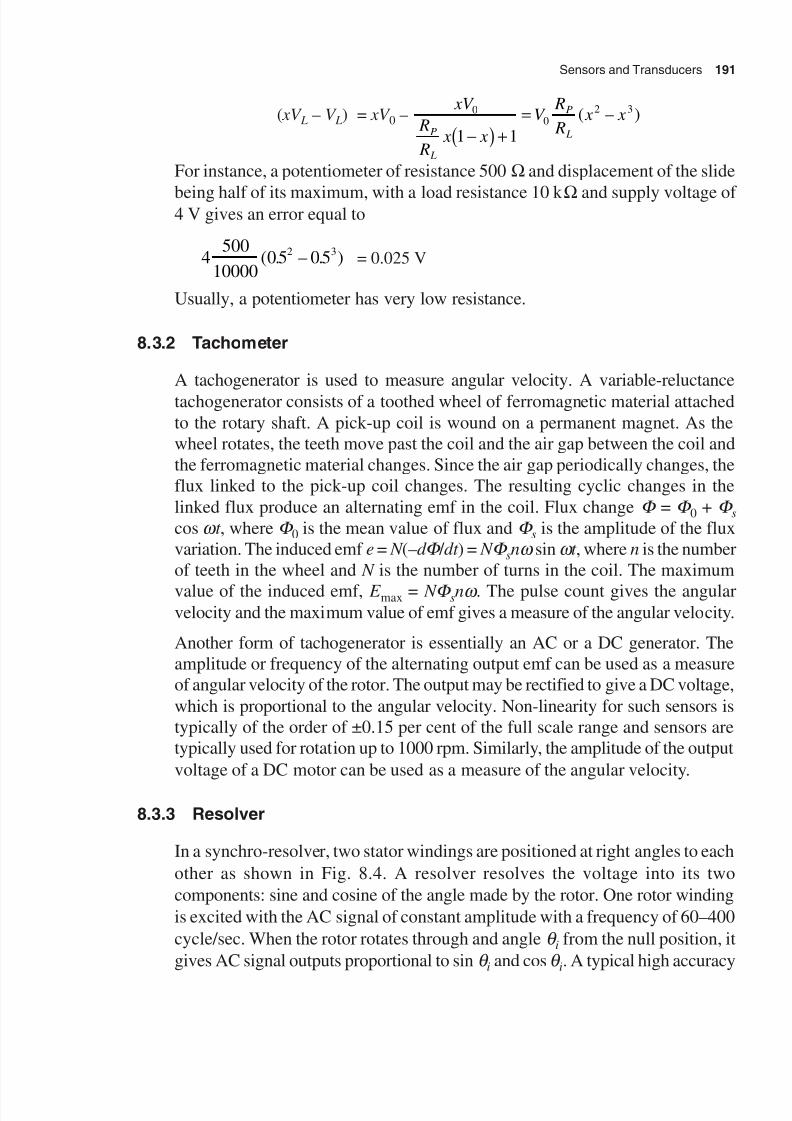
8/11/2019 Introduction to Mechatronics - Appuu Kuttan.pdf
http://slidepdf.com/reader/full/introduction-to-mechatronics-appuu-kuttanpdf 200/345
Sensors and Transducers 191
( xV L – V L) = xV 0 – xV
R
R x x
V R
R x x
P
L
P
L
00
2 3
1 1- +
=
( – )
For instance, a potentiometer of resistance 500 W and displacement of the slide
being half of its maximum, with a load resistance 10 k W and supply voltage of4 V gives an error equal to
4500
1000005 05
2 3( . – . ) = 0.025 V
Usually, a potentiometer has very low resistance.
8.3.2 Tachometer
A tachogenerator is used to measure angular velocity. A variable-reluctance
tachogenerator consists of a toothed wheel of ferromagnetic material attached
to the rotary shaft. A pick-up coil is wound on a permanent magnet. As the
wheel rotates, the teeth move past the coil and the air gap between the coil and
the ferromagnetic material changes. Since the air gap periodically changes, the
flux linked to the pick-up coil changes. The resulting cyclic changes in the
linked flux produce an alternating emf in the coil. Flux change F = F 0 + F scos w t , where F 0 is the mean value of flux and F s is the amplitude of the flux
variation. The induced emf e = N (–d F / dt ) = N F snw sin w t , where n is the number
of teeth in the wheel and N is the number of turns in the coil. The maximum
value of the induced emf, E max = N F snw . The pulse count gives the angularvelocity and the maximum value of emf gives a measure of the angular velocity.
Another form of tachogenerator is essentially an AC or a DC generator. The
amplitude or frequency of the alternating output emf can be used as a measure
of angular velocity of the rotor. The output may be rectified to give a DC voltage,
which is proportional to the angular velocity. Non-linearity for such sensors is
typically of the order of ±0.15 per cent of the full scale range and sensors are
typically used for rotation up to 1000 rpm. Similarly, the amplitude of the output
voltage of a DC motor can be used as a measure of the angular velocity.
8.3.3 Resolver
In a synchro-resolver, two stator windings are positioned at right angles to each
other as shown in Fig. 8.4. A resolver resolves the voltage into its two
components: sine and cosine of the angle made by the rotor. One rotor winding
is excited with the AC signal of constant amplitude with a frequency of 60–400
cycle/sec. When the rotor rotates through and angle q i from the null position, it
gives AC signal outputs proportional to sin q i and cos q i. A typical high accuracy

8/11/2019 Introduction to Mechatronics - Appuu Kuttan.pdf
http://slidepdf.com/reader/full/introduction-to-mechatronics-appuu-kuttanpdf 201/345
192 Introduction to Mechatronics
resolver has an excitation voltage of 26 V at the maximum operating frequency
of 400 cycles/sec. The connection to the rotor is made by the brushes and slip
rings. A digitizer converts the input signal and the output from two stator
windings into a digital signal, which gives the exact rotation of the rotor.
Resolvers are rugged and operate on a wide temperature range. They can operateat very low speeds. The main disadvantage of the resolver is the requirement of
oscillator and digital converter. These requirements make it costly as well.
Oscillator
Stator
Digitalconverter
Digitaloutput
Fig. 8.4 Resolver
8.3.4 Optical Encoder
An encoder is a device that provides digital output as a result of a linear orangular displacement. Based on the position of the encoder, it is grouped intotwo categories, namely, incremental and absolute encoders. The incrementalencoder gives the direct change in rotation from the same datum position whereasthe absolute encoder gives the actual angular position. Figure 8.5(a) shows thebasic form of an incremental encoder used for the measurement of angulardisplacement. In this set-up a beam of light passes through slots in a disk and is
detected by a suitable light sensor. When the disk is rotated, the sensor producesa pulsed output, with the number of pulses being proportional to the angle throughwhich the disk rotates. Thus the angular position of the disk in the shaft rotationcan be determined. In practice, concentric tracks with these sensors are used.The inner track has just one hole and is used to locate the home position of thedisk. The other two tracks are used to determine the direction of rotation of the
shaft. This is achieved by off-setting the two track holes into one and a halfwidth of the hole. Figure 8.5(b) shows the basic form of an absolute encoder forthe measurement of angular displacement. This encoder gives an output in theform of a binary number of several digits and each digit represents a particular
angular position.
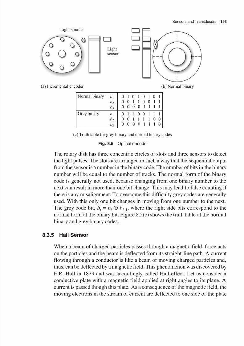
8/11/2019 Introduction to Mechatronics - Appuu Kuttan.pdf
http://slidepdf.com/reader/full/introduction-to-mechatronics-appuu-kuttanpdf 202/345
Sensors and Transducers 193
Light source
Lightsensor
(a) Incremental encoder (b) Normal binary
Normal binary b1
b2
b3
000
100
010
110
001
101
011
111
Grey binary b1
b2b3
0
00
1
00
1
10
0
10
0
11
1
11
1
01
1
00
(c) Truth table for grey binary and normal binary codes
Fig. 8.5 Optical encoder
The rotary disk has three concentric circles of slots and three sensors to detect
the light pulses. The slots are arranged in such a way that the sequential output
from the sensor is a number in the binary code. The number of bits in the binary
number will be equal to the number of tracks. The normal form of the binary
code is generally not used, because changing from one binary number to thenext can result in more than one bit change. This may lead to false counting if
there is any misalignment. To overcome this difficulty grey codes are generally
used. With this only one bit changes in moving from one number to the next.
The grey code bit, bi = bi ≈ bi–1, where the right side bits correspond to the
normal form of the binary bit. Figure 8.5(c) shows the truth table of the normal
binary and grey binary codes.
8.3.5 Hall Sensor
When a beam of charged particles passes through a magnetic field, force acts
on the particles and the beam is deflected from its straight-line path. A current
flowing through a conductor is like a beam of moving charged particles and,
thus, can be deflected by a magnetic field. This phenomenon was discovered by
E.R. Hall in 1879 and was accordingly called Hall effect. Let us consider a
conductive plate with a magnetic field applied at right angles to its plane. A
current is passed though this plate. As a consequence of the magnetic field, the
moving electrons in the stream of current are deflected to one side of the plate

8/11/2019 Introduction to Mechatronics - Appuu Kuttan.pdf
http://slidepdf.com/reader/full/introduction-to-mechatronics-appuu-kuttanpdf 203/345
194 Introduction to Mechatronics
and that side becomes negatively charged. The opposite side of the plate becomes
positively charged, since the electrons are directed away from it. This charge
separation produces an electric field in the plate material. The charge separation
continues until the force on the charged particles from the electric field just
balances the force produced by the magnetic field. The result is a transverse
potential difference V, which is given by
V =K BI
t
H
where B is the magnetic flux density at right angles to the plate, I is the current
passing through the plate, t is the thickness of the plate, and K H is the constant
called the Hall coefficient. Thus, if a constant current source is used with a particular
sensor, the Hall voltage is the measure of the magnetic flux density. The Hall
effect sensor is immune to environment contamination and can be used under
severe service conditions. A Hall generator is used to sense the rotary shaft speedor position. It is most frequently used in brushless permanent magnetic DC motors.
Figure 8.6 illustrates the working principle of the Hall sensor.
Current
Inducedvoltage
S
N
Fig. 8.6 Hall sensor
The Hall sensor uses a small, semi-conducting chip of indium arsenide or indium
arsenide oxide. The chip is not more than 0.025 mm thick. It is usually enclosed
in a plastic envelope. Two of its opposite edges are connected to a constant DCvoltage source. The other two edges are connected to an amplifier to transmit
the Hall voltage, which is generated as soon as the chip is exposed to the magnetic
field.
8.3.6 Moire’s Fringe Sensor
The linear or angular position of any link of a mechatronic system can be detected
by using Moire’s fringe grating. In the linear grating, a precision scale is engraved
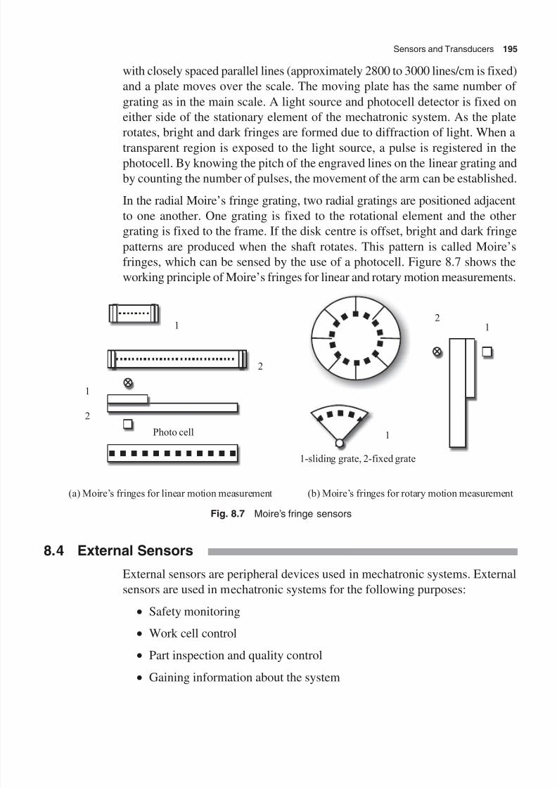
8/11/2019 Introduction to Mechatronics - Appuu Kuttan.pdf
http://slidepdf.com/reader/full/introduction-to-mechatronics-appuu-kuttanpdf 204/345
Sensors and Transducers 195
with closely spaced parallel lines (approximately 2800 to 3000 lines/cm is fixed)
and a plate moves over the scale. The moving plate has the same number of
grating as in the main scale. A light source and photocell detector is fixed on
either side of the stationary element of the mechatronic system. As the plate
rotates, bright and dark fringes are formed due to diffraction of light. When atransparent region is exposed to the light source, a pulse is registered in the
photocell. By knowing the pitch of the engraved lines on the linear grating and
by counting the number of pulses, the movement of the arm can be established.
In the radial Moire’s fringe grating, two radial gratings are positioned adjacent
to one another. One grating is fixed to the rotational element and the other
grating is fixed to the frame. If the disk centre is offset, bright and dark fringe
patterns are produced when the shaft rotates. This pattern is called Moire’s
fringes, which can be sensed by the use of a photocell. Figure 8.7 shows the
working principle of Moire’s fringes for linear and rotary motion measurements.
1
2
1
2
Photo cell
12
1
1-sliding grate, 2-fixed grate
(a) Moire’s fringes for linear motion measurement (b) Moire’s fringes for rotary motion measurement
Fig. 8.7 Moire’s fringe sensors
8.4 External SensorsExternal sensors are peripheral devices used in mechatronic systems. External
sensors are used in mechatronic systems for the following purposes:
∑ Safety monitoring
∑ Work cell control
∑ Part inspection and quality control
∑ Gaining information about the system

8/11/2019 Introduction to Mechatronics - Appuu Kuttan.pdf
http://slidepdf.com/reader/full/introduction-to-mechatronics-appuu-kuttanpdf 205/345
196 Introduction to Mechatronics
There are many types of external sensors such as proximity sensors, range finders,
tactile sensors, machine vision sensors, and force sensors. We will discuss these
in the following sub-sections.
8.4.1 Proximity Sensors
Proximity sensors are the devices that are used to locate objects in close
proximity. The closeness of the object, for which the sensor can sense its presence,
depends on the device used for the purpose. The distance can be anywhere
between several millimetres to several metres. A variety of technologies are
available for designing proximity and range sensors. These technologies include
optical devices, acoustics, electrical field techniques, and pneumatic pressure
drop methods.
Optical proximity sensors can be designed to suit operations in the visible or
invisible (infrared) light. Infrared sensors may be active or passive. The active
sensors send out an infrared beam and respond to the deflection of the beam
against the target. The infrared reflection sensor using an incandescent light
source is a common device that is commercially available. The active infrared
sensor can be used to indicate not only the presence but also the location of a
part/object. Passive infrared sensors are simple devices which detect the presence
of infrared radiation in the environment. They are often used in security systems
to detect the presence of bodies giving off heat within the range of the sensor.
These sensor systems are effective at covering large areas in building interiors.
Acoustic devices can be used as proximity sensors. Ultrasonic frequencies above
20000 Hz are often used in such devices. One type of acoustical proximity
sensor uses a cylindrical, open ended chamber with an acoustic emitter at the
closed end of the chamber. The emitter sets up a pattern of standing waves in
the cavity, which is altered by the presence of an object near the open end. A
microphone located in the well of the chamber is used to sense the change in the
sound pattern. This kind of sensors can also be used as range finders.
There are various forms of switches that can be activated by the proximity of an
object. The proximity sensors in such switches sense the object and give anoutput which may indicate either an on state or an off state. The microswitch is
a small electrical switch and requires a small physical contact and a small
operating force to close the contacts.
Pneumatic sensors involve the use of compressed air. In this device the
proximity of an object is transformed into a change in air pressure. Figure 8.8(a)
shows the basic form of such a sensor. Low pressure is allowed to escape through
a port in front of the sensor. This displaces the air in the absence of any closeby
object, thereby reducing the pressure in the vicinity of the sensor output port.

8/11/2019 Introduction to Mechatronics - Appuu Kuttan.pdf
http://slidepdf.com/reader/full/introduction-to-mechatronics-appuu-kuttanpdf 206/345
Sensors and Transducers 197
If there is a closeby object, the air cannot so readily escape and the result is that
pressure increases in the sensor output port. The output pressure from the sensor,
thus, depends on the proximity of the object. Such sensors are used for the
measurement of displacements of a fraction of a millimetre in range which
typically is 2–12 mm.Proximity sensors involving the use of electrical field are commercially available.
Two types of sensors in this category are eddy current proximity sensors and
magnetic field sensors. If a coil is fed with an alternating current input, an
alternating magnetic field is produced. If there is a metal object in close proximity
to this alternating magnetic field, then eddy currents are induced in it. The eddy
currents themselves produce magnetic field. This distorts the magnetic field
responsible for their production. As a result, the impedance of the coil changes
the amplitude of the alternating current. At some preset level, this change can
be used to trigger a switch. Figure 8.8(b) shows the basic form of the eddycurrent proximity sensor. It is used for detecting non-magnetic but conductive
materials. These sensors have the advantage of being relatively inexpensive,
smaller size, high reliability, and high sensitivity to small displacement.
Magnetic field proximity sensors are relatively simple and can be made using a
permanent magnet. The magnet can be made a part of the object being detected
or can be part of the sensor device. It can only be used for the detection of metal
objects and is best for ferrous metal.
Low pressure air
Obstacle
Electromagnet
(a) Pneumatic proximity sensor (b) Eddy current proximity sensor
Fig. 8.8 Proximity sensors
8.4.2 Range Finder
Range sensing is concerned with detecting how near or how far a component is
from the sensing position. Range sensing (also called distance sensing) works
on the noncontact analog technique. Short range sensing may be accomplished
with the electrical capacitance, inductive or magnetic technique. They can be
made active with a range of few millimetres to 400 mm.

8/11/2019 Introduction to Mechatronics - Appuu Kuttan.pdf
http://slidepdf.com/reader/full/introduction-to-mechatronics-appuu-kuttanpdf 207/345
198 Introduction to Mechatronics
Long range sensing usually involves transmitting energy waves and a receiver
situated on the sensing device receives the reflected waves to determine the
distance. The time taken for energy waves to reach the receiver is used to find
out the distance between the sensing device and the object. Continuous ranging
can be achieved by transmitting energy waves towards the target and detectingthem when these are reflected back. This principle is well established in radar
and sonar techniques. The use of laser for range sensing for long distance ranging
has been used for long and is now a well established technique for long range
sensing.
Figure 8.9(a) illustrates the simple configuration of a laser-based triangular range
finder. In this case, a single mode He-Ne laser is used. The laser beam impinges
on the centre of the mirror that rotates at a fixed speed so that the given plane is
Fig. 8.9 Range finder
8/11/2019 Introduction to Mechatronics - Appuu Kuttan.pdf
http://slidepdf.com/reader/full/introduction-to-mechatronics-appuu-kuttanpdf 208/345
Sensors and Transducers 199
continuously scanned. The distance between the arm of rotation and the
photodetector constitutes the base line of the range finder. The development of
the solid state laser diode and the ease of interfacing the optical sensor to the
microcomputer have led to the design and implementation of a compact and
accurate optical range finder. An ideal range finder should meet the followingrequirements:
1. The sensor must be capable of gauging the distances between 1 cm to 1 m
to meet with a resolution of 1 mm.
2. The size of the sensor should be of the order of few cubic inches, so that
it can be mounted on any mechatronics system.
3. The sensor should be relatively insensitive to the degree of effectiveness
of the object.
Figure 8.9(b) illustrates the general configuration of the laser beam triangulation.
In this set-up, a narrow collimated ray is directed towards the target with the
help of a set of collimated lens. The beam impinges on the cube of the mirror
that can rotate at a fixed range, so that the given plane is continuously scanned.
A position-sensitive photodetector is placed in the scanning plane; the distance
between the axis of rotation of the mirror and centre of the photodetector
constitutes the baseline of the range finder.
8.4.3 Tactile Sensors
Tactile sensing means sensing through touch. In its widest context, tactile sensing
can be taken to mean any sensing wherein a contact is involved. The simplest
form of such a device is a square or rectangular array in which sensors are
arranged in rows and columns. They are commonly called matured sensors.
Each individual sensor is activated when brought into contact with the object.
By detecting the active sensors or by analysing the magnitude of the output
signal of the sensors, the input to the component being touched can be
determined. This input is then compared with the previously stored input
information to determine the size and shape of the component. Basically, thereare three designs available for tactile sensors. These are the conductive skin,
large scale integrated (LSI) circuit tactile sensor, and magnetic resistive skin.
Figure 8.10 illustrates the artificial skin or conductive membrane which was
developed at the MIT laboratory. There are 256 tactile sensors in a space of the
size of the finger tip. Each sensor has an area of 0.0163 cm2 and is a multi-layer
construction of different materials. The top layer is a sheet of elastomer
conductive silicon rubber impregnated within a graphite or silver layer of

8/11/2019 Introduction to Mechatronics - Appuu Kuttan.pdf
http://slidepdf.com/reader/full/introduction-to-mechatronics-appuu-kuttanpdf 209/345
200 Introduction to Mechatronics
approximately 0.25 mm thickness. The bottom layer is a printed circuit board
(PCB), etched into fine parallel lines so that it conducts in only one direction.
The sensitivity of the sensor depends on the construction of the middle layer,
which consists of a fine mesh of either nylon or non-conductive paint. Wires are
connected to the PCB at the edge of the array. The array is scanned by applyingvoltage to one row at a time. When an object is placed on the conductive
membrane, the conductive membrane pierces through the mesh and short circuits
the conductance of the wire and hence the current flow through the wire varies.
Measurement of the current flow in each row of the wire identifies the object.
Fine mesh
Conductive membrane
625 10 mmSquare piece
–10
Fig. 8.10 Artificial skin
Scientists at the NASA Jet Propulsion Laboratory have been working on the
design of large scale integrated (LSI) circuits as tactile sensors. This type of
sensor combines the function of transduction computation and communication.
The basic concept of the LSI circuit design is shown in Fig. 8.11. The LSI wafer
concept uses an array of tactile sensors with sensing materials connected directly
to the computing element of the wafer. Such an arrangement reduces the rows
of sensing data and sends the resulting signal to control the computer. A number
of functions are thus combined. The signal bandwidth, number of connectionwires, weights, and power consumption are reduced, while a high tactile
resolution is achieved. The grasping force, touch pattern, contact area, and slipper
can be extracted from the reading. The exposed surface of the LSI wafer contains
an array of pairs of electrodes covered by a sheet of electrically conductive
rubber. When the rubber sheet is deformed by touch, its resistivity varies locally.
The current passing through the sheet between the pair of electrodes is indicated
by the local contact pressure. An assembled electrode pair is the computational
element consisting of an analog comparator, an adding register, and accumulators.

8/11/2019 Introduction to Mechatronics - Appuu Kuttan.pdf
http://slidepdf.com/reader/full/introduction-to-mechatronics-appuu-kuttanpdf 210/345
8/11/2019 Introduction to Mechatronics - Appuu Kuttan.pdf
http://slidepdf.com/reader/full/introduction-to-mechatronics-appuu-kuttanpdf 211/345
202 Introduction to Mechatronics
8.4.4 Machine Vision
Machine vision means the capture of an image in real time via some form of a
camera system and its conversion into a form that can be fed into and analysed
by a computer system. The conversion process is called digitization of the image.
The processes of image capture, digitization, and data analysis should be enough
to enable the mechatronic systems to respond to the analysed image and take
appropriate action during performance.
The operation of a vision system consists of three functions:
∑ Sensing and digitizing image data
∑ Image process and analysis
∑ Image interpretation
Sensing and digitizing functions involve the input of the vision data by means
of a camera focused on the screen of interest. Special lighting techniques are
frequently used to obtain the image of sufficient contrast for later processing.
The image received by a camera is typically digitized and stored in computer
memory. The digital vision is called a frame grabber. These devices are capable
of digitizing images at a rate of 30 frames/sec. A frame consists of a matrix of
data representing projection(s) of the scene sensed by the camera. The elements
of the matrix are called picture elements or pixels. The number of pixels is
determined by a sampling process performed on each image frame. A single
pixel is the projection of the small portion of the scene, which reduces to a
single value. Usually 236 ¥ 236 pixels will be there in an area of 1 cm2. The
value from a single pixel is a measure of high intensity for that element of the
scan. The pixel's intensity is converted into a digital value.
Image capture is achieved through the vision camera. Two types of cameras
used, namely, vidicon camera and coupled charged device (CCD). Figure 8.13
illustrates the working of the vidicon camera. In this camera system, the lens
forms an image on the glass face plate of the camera. The face plate has its
inner surface coated with two layers. The first layer consists of a transparentsignal electrode film deposited on the face plate of the inner surface. The second
layer is a thin photosensitive material deposited over the conducting film. The
photosensitive layer consists of a high density photosensitive material in a small
layer area. These areas are similar to pixels, and each rear pixel generates a
decreasing electrical resistance in response to increasing illumination. An
electrical charge is thus generated corresponding to the image formed on the
face plate. The charge accumulated for an area is a function of the intensity for
impinging light over the span feed time. Once light-sensitive scan is built up,

8/11/2019 Introduction to Mechatronics - Appuu Kuttan.pdf
http://slidepdf.com/reader/full/introduction-to-mechatronics-appuu-kuttanpdf 212/345
Sensors and Transducers 203
the charge is read out to produce the vedicon signal. This is accomplished by
scanning the photosensitive layer by an electron beam. The scanning is controlled
by a deflection coil mounted along the length of the tube. For accumulated
positive charge, the electron beam deposits enough electrons to neutralize the
charge. An equal number of electrons flow to cause current to flow at the videosignal electrode. The magnitude of the current signal in each pixel is proportional
to the intensity of light and the pixel size. The current is then directed through
a load resistor, which develops a signal voltage, which is further amplified and
analysed. Raster scanning eliminates the need to consider time at each area by
making scan time equal for all areas. Only the line intensity of the impinging
light is considered. Raster scanning is typically done by scanning the electrode
beam from left to right and from top to bottom. The output of the camera is a
continuous voltage signal for each line scanned. The voltage signal for each
scanned line is subsequently sampled and quantified, resulting in a series ofversion processes for the complete screen. This finally gives two-dimensional
arrays of picture elements. Typically a single pixel is quantified between 6 and
8 bit by the analog-to-digital converter.
Horizontal deflection
Vertical deflection
Lense
ObjectElectron gun
Fig. 8.13 Vidicon camera
The coupled charge device (CCD) is a solid state camera. In this technology the
image is projected by a camera on a CCD, which detects, stores and read outs
the accumulated charges generated by the light on each portion of the image.
The light detection occurs through the absorption of light on a photoconductive
substrate of silicon. Charges accumulate under positive controlled electrodes in
isolated wells due to voltage applied to the controlled electrodes. Each isolated
well represents one pixel and can be transferred to an output storage resistor by
varying the voltage on the metal control electrode. Figure 8.14 illustrates the
working of a CCD.

8/11/2019 Introduction to Mechatronics - Appuu Kuttan.pdf
http://slidepdf.com/reader/full/introduction-to-mechatronics-appuu-kuttanpdf 213/345
204 Introduction to Mechatronics
Metal electrode
Light
Insulator on silicon wafer
P-type silicon wafer
Fig. 8.14 Coupled charge device
In most vision systems video signal is digitized by an analog-to-digital converter
and stored in fine buffer for subsequent computer analysis. The resolution of
the device is determined by the sampling rate of the analog-to-digital converter.
The frame grabber is an image storing and computational device which stores a
given pixel array. A digital representation of the image means that the imageinformation is stored sequentially as a binary bit pattern in computer memory.
The grey level is a measure of the pixel brightness. The simplex level of each
individual bit can be interpreted as either bright, which is set to binary ‘1’, or
dark, which is set to the binary ‘0’. Grey scaling refers to digitization of 256
shades of brightness using 8 bit coding for each pixel. It resolves to determine
the possible number of quantified levels of assessment by the video analog-to-
digital converter to each pixel to represents its brightness value. The number
usually is 1064 or 256 shades of grey.
The computer must be programmed to operate on the stored digital image foruse as per the needs of the application. This is a substantial task, considering
the large amounts of data that must be analysed. There are various techniques to
reduce the magnitude of the image processing problems. These techniques
include the following:
∑ Image data reduction
∑ Segmentation
∑ Feature extraction
∑ Object recognition
In the image data reduction technique, the objective is to reduce the volume of
data. Two schemes have found common use, namely, digital conversion andwindowing. Digital conversion reduces the number of grey levels used by themachine vision system. Windowing involves uses only a portion of the total
image stored in the frame buffer for image processing and analysis. This portionis called the window. In this technique the image is processed in a portion-by-
portion manner.

8/11/2019 Introduction to Mechatronics - Appuu Kuttan.pdf
http://slidepdf.com/reader/full/introduction-to-mechatronics-appuu-kuttanpdf 214/345
Sensors and Transducers 205
Segmentation is a general term and applies to various methods of data reduction.
The objective of segmentation is to grab areas of an image having similar features,
singular edges, areas, etc. There are many ways to segment an image such as
thresholding, region growing, and edge detection. Thresholding is a binary
conversion technique in which each pixel is converted into a binary value, either
black or white. Region growing is a collection of segmentation techniques in
which pixels are grouped in regions, called grid elements, based on attribute
similarities. This technique creates runs of 1's and 0's and is often used as the
first pass analysis to partition the image into identification segments or blobs.
For a simple image such as a dark blob on a light background, the run technique
can provide useful information. For more complex images this technique may
not provide an adequate portion of an image into a set of useful regions. Such
regions might contain pixels that are connected to each other and have similar
attributes. Edge detection considers the intensity change that occurs in the pixels
of the boundary or edge of a part.
Feature extraction is usually accomplished by means of features that uniquely
characterize the object. Some features of the object that can be used in machine
vision include the area, diameter, perimeter, etc. A feature is a parameter that
permits ease of comparison and identification.
Identification is accomplished using the extract feature information. The object
recognition algorithm must be powerful enough to uniquely identify the object.
The object recognition method may be implemented in two different ways:
1. Template match technique
2. Structural technique
The template match technique is a subset of the more general statistical pattern
recognition technique that serves to classify the object in an image into a
predetermined category. The basic objective in template matching is to match
its object with a stored pattern feature set defined, called model template. This
technique is suited to applications that do not need a large number of model
templates. The structural technique of pattern recognition considers the
relationships between features and edges of an object. It can be computationallytime consuming for complete pattern recognition. It is often more appropriate
for searching a simple region or edge within an image. These simpler regions
can then be used to extract the required features.
8.4.5 Force Sensors
A spring balance is an example of a force sensor in which a force or weight is
applied to cause displacement. The resultant displacement gives the measure of

8/11/2019 Introduction to Mechatronics - Appuu Kuttan.pdf
http://slidepdf.com/reader/full/introduction-to-mechatronics-appuu-kuttanpdf 215/345
206 Introduction to Mechatronics
the force applied. The force applied can be static or dynamic. Force sensors are
analog in operation and are sensitive to the direction of force applied. There are
six types of forces that may require sensing. These are given below.
∑ Tensile force
∑ Compressive force
∑ Shear force
∑ Torsional force
∑ Bending force
∑ Frictional force
There are many techniques used in sensing these forces. Some of these techniques
are direct and others indirect. The selection of a particular technique dependson the type and magnitude of the force and mode of its application.
A commonly used form of the force-measuring transducer is based on the use
of electrical resistance and strain gauge monitor. Application of force produces
strain in some members when they are stretched or compressed. This strain
causes them to bend. This arrangement is generally referred to as a load cell.
Figure 8.15 shows an example of such a cell. It consists of a cylindrical tube.
Strain gauges are attached to this tube when force is applied to compress it.
Then the strain gauges give a resistance change, which is a measure of thestrain and hence the applied force. Typically such load cells are used for forces
up to 10 MN. Strain gauge load cells are used for small forces varying from 0 to
5N up to 0 to 50 kN. Uncertainties in the sensor are typically a non-linearity
error of about ±0.03% of full range, hysteresis error ±0.02% of full range and
repeatability error ±0.02% of full range.
An unknown force may be measured by
1. Balancing against the known gravitational force on a standard mass
2. Measuring the acceleration of a body of known mass to which the unknown
force is applied
3. Balancing against a magnetic force developed by the interaction of a current
carrying coil and magnet
4. Transducing the force to a pressure and measuring the pressure
5. Applying the force to some elastic member and measuring the resulting
deflection

8/11/2019 Introduction to Mechatronics - Appuu Kuttan.pdf
http://slidepdf.com/reader/full/introduction-to-mechatronics-appuu-kuttanpdf 216/345
Sensors and Transducers 207
Torque transmission to a rotating shaft generally involves both the source of
power and a sink. Torque-measuring devices are called dynamometers. These
devices may be generative type, absorption dynamometer, and transmission
dynamometer. The transmission dynamometer is based on the strain gauge
arrangement.Force
Strain gauges
Fig. 8.15 Load sensor
8.5 Microsensors
The rapid advances in micro-fabrication technologies have led to the
development of many microsensors. Microsensors are the most widely used
mechatronic devices today. A smart sensor unit performs the following functions:
automatic calibration, interference signal reduction, parasite effect compensation,offset correction, and self testing. All these functions make the sensor unit an
intelligent micro-system.
Many types of microsensors are used to perform various functions in a variety
of industries. These are generally used to measure physical quantities. We will
discuss and explain the working principle of some of the microsensors in the
following sections.
8.5.1 Strain Gauges
Strain gauges are resistive pick ups used as transducers. The resistance of the
gauge changes in accordance with the strain, which in turn can be used for the
measurement of input signals such as load or stress. The strain gauge consists
of a metallic filament of approximately 0.03 mm diameter, which is sandwiched
between thin layers of paper or epoxy resins. When load is applied to the surface
of the elastic member where the strain gauges are mounted, a change in the
length of the wire results. This change leads to a change in the resistance. This
change in resistance can be measured with the help of a conventional Wheatstone
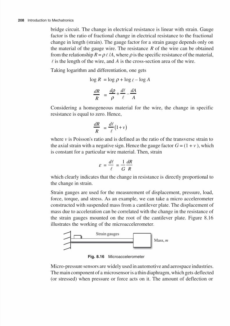
8/11/2019 Introduction to Mechatronics - Appuu Kuttan.pdf
http://slidepdf.com/reader/full/introduction-to-mechatronics-appuu-kuttanpdf 217/345
208 Introduction to Mechatronics
bridge circuit. The change in electrical resistance is linear with strain. Gauge
factor is the ratio of fractional change in electrical resistance to the fractional
change in length (strain). The gauge factor for a strain gauge depends only on
the material of the gauge wire. The resistance R of the wire can be obtained
from the relationship R = r / A, where r is the specific resistance of the material,
is the length of the wire, and A is the cross-section area of the wire.
Taking logarithm and differentiation, one gets
log R = log r + log – log A
dR
R =
d d dA
A
r
r +
–
Considering a homogeneous material for the wire, the change in specific
resistance is equal to zero. Hence,
dR
R=
d v
1+
where v is Poisson's ratio and is defined as the ratio of the transverse strain to
the axial strain with a negative sign. Hence the gauge factor G = (1 + v ), which
is constant for a particular wire material. Then, strain
e = d
=
1
G
dR
Rwhich clearly indicates that the change in resistance is directly proportional to
the change in strain.
Strain gauges are used for the measurement of displacement, pressure, load,
force, torque, and stress. As an example, we can take a micro accelerometer
constructed with suspended mass from a cantilever plate. The displacement of
mass due to acceleration can be correlated with the change in the resistance of
the strain gauges mounted on the root of the cantilever plate. Figure 8.16
illustrates the working of the microaccelerometer.
Strain gauges
Mass, m
Fig. 8.16 Microaccelerometer
Micro-pressure sensors are widely used in automotive and aerospace industries.
The main component of a microsensor is a thin diaphragm, which gets deflected
(or stressed) when pressure or force acts on it. The amount of deflection or

8/11/2019 Introduction to Mechatronics - Appuu Kuttan.pdf
http://slidepdf.com/reader/full/introduction-to-mechatronics-appuu-kuttanpdf 218/345
Sensors and Transducers 209
stress induced in the diaphragm deformation is then converted into an electricalsignal output through transduction. There are generally two types of pressuresensors: absolute pressure and gauge pressure sensors. The absolute pressure
sensor has an evacuated cavity on one side of the diaphragm. The measuredpressure is the absolute value with vacuum as the reference pressure. In the
absolute pressure type, nano-evacuation is necessary. Figure 8.17 illustrates amicro-pressure sensor. The top view of the silicon die shows four piezoresistorsplanted beneath the surface of the silicon die. These piezoresistors convert thestresses/deflection induced in the silicon diaphragm by the applied pressure
into a charge of electrical resistance, which is then converted into voltage outputby a Wheatstone bridge circuit. The piezoresistors are essentially miniaturizedsemiconductor strain gauges which can produce the charge of electrical resistanceinduced by the mechanical stresses output from the Wheatstone bridge.
V o = V i R
R R
R
R R
1
1 4
3
2 3+ +
–
where V i and V o are the input and output voltages of the Wheatstone bridge,
respectively. R4
R1 R3
Silicon die withdiaphragm
Fluid inlet
Fig. 8.17 Micro-pressure sensor
8.5.2 Thermocouples
Thermocouples are employed as temperature sensing elements. Basic principle
of a thermocouple is seeback effect. When two different metals are joined
together and the temperatures at the two junctions are different, then a potential
difference occurs across the junctions. This phenomenon is known as the Seebeck

8/11/2019 Introduction to Mechatronics - Appuu Kuttan.pdf
http://slidepdf.com/reader/full/introduction-to-mechatronics-appuu-kuttanpdf 219/345
210 Introduction to Mechatronics
effect. The reverse of this phenomenon is called the Peltier effect. When a voltage
is applied to this kind of circuit, the temperature at one junction is lower and at
the other junction is higher than the ambient temperature. The principle of the
Peltier effect is used for micro-space air conditioning. The Thomson effect states
that there is a temperature gradient in a conductor when current is passed throughthe conductor. The principles of the Seeback effect, Peltier effect, and Thomson
effect are effectively used in microsystems application. A thermocouple used
for temperature measurement is an example of the application of the Seeback
effect. Since there is a temperature difference between the two junctions of a
thermocouple, the value of emf, E , depends on the two metals concerned and
the temperature T of the junctions. Mathematically, E = aT + bT 2, where a and
b are constants. Some commonly used thermocouple materials are iron/
constantam, chromel/alumal, copper/constantam, and platinum/platinum-
rhodium alloys.Micro-thermopile is a more realistic solution for miniaturized heat sensing. It
operates with both hot and cold junctions. In this case, the thermocouple is in
parallel and the voltage output is in series. Materials used for a thermopile are
the same as those used for a thermocouple. The voltage output from a thermopile
can be obtained from the expression DV = N b DT, where N is the number of
thermocouples, b is the thermoelectric power, and DT is the temperature
difference between the two junctions. Figure 8.18 represents a micro-thermopile
with total 32 polysilicon volt thermocouples in the thermopile. The dimensions
of this silicon chip are 2.6 mm ¥ 3.6 mm ¥ 3.6 mm. A typical output signal of 100 mV can be obtained from a 500K black body source of Q = 0.29 W/cm
2
with a response time of about 50 ms.
Fig. 8.18 Schematic diagrams of micro-thermopile and thermocouple

8/11/2019 Introduction to Mechatronics - Appuu Kuttan.pdf
http://slidepdf.com/reader/full/introduction-to-mechatronics-appuu-kuttanpdf 220/345
Sensors and Transducers 211
8.5.3 Acoustic Wave Sensor
The principal application of an acoustic wave sensor is to measure chemical
composition in a gas. Each sensor generates acoustic waves by converting
mechanical energy into electrical acoustic waves. These devices are also used
to activate or regulate the fluid flow through micro-fluidic systems. The actuation
energy for this type of sensors is provided by piezoelectric and magnetostriction
mechanisms. The former mechanism is a more popular method for generating
acoustic waves. Piezoelectricity is a common means for transducing mechanical
energy into electrical energy and vice versa.
8.5.4 Biomedical Sensors and Biosensors
Biosensors present great challenges to engineers as the designing and
manufacturing of this type of sensors requires considerable knowledge andexperience in molecular biology as well as physical chemistry. Basically two
types of sensors are used in biomedical applications:
∑ Biomedical sensors
∑ Biosensors
Biomedical sensors are used to detect biological substances. As against this
class of sensors, biosensors are measuring device that use biological element(s)
such as antibodies or enzymes for sensing activities. Biomedical sensors and
biosensors are discussed in detail in Chapter 11.
8.5.5 Chemical Sensors
Chemical sensors are used to identify chemical compounds such as various gas
species. The working principle behind these sensors is very simple. We know
that many materials are sensitive to chemical attacks. For example, most
materials are vulnerable to oxidation when exposed to air for a long time. A
significant oxide layer built up over a metal surface can change material
properties, such as the electrical resistance, of the original metal. Materialsensitivity to specific chemicals is used as a basic principle for many chemical
sensors. Three types of chemical sensors are in use. They are chemi-resistors,
chemi-capacitors, and metal-oxide gas sensors. Organic polymers are used with
an embedded metal sensor. These polymers can cause a change in the electrical
conductivity of the metal when it is exposed to certain gases. For example, a
special polymer called phthalocyamine is used with copper to sense ammonia
and nitrogen dioxide gases. Some polymers can also be used as dielectric
materials in a capacitor. The exposure of these polymers to certain gases alters
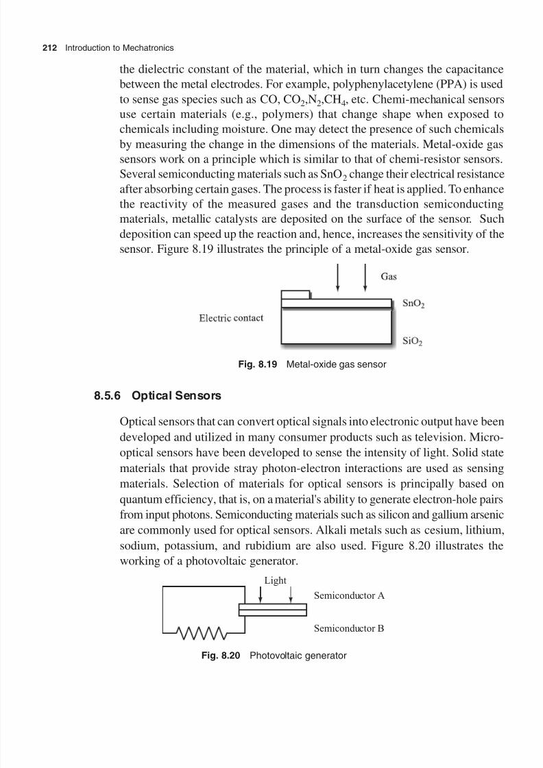
8/11/2019 Introduction to Mechatronics - Appuu Kuttan.pdf
http://slidepdf.com/reader/full/introduction-to-mechatronics-appuu-kuttanpdf 221/345
212 Introduction to Mechatronics
the dielectric constant of the material, which in turn changes the capacitance
between the metal electrodes. For example, polyphenylacetylene (PPA) is used
to sense gas species such as CO, CO2,N2,CH4, etc. Chemi-mechanical sensors
use certain materials (e.g., polymers) that change shape when exposed to
chemicals including moisture. One may detect the presence of such chemicalsby measuring the change in the dimensions of the materials. Metal-oxide gas
sensors work on a principle which is similar to that of chemi-resistor sensors.
Several semiconducting materials such as SnO2 change their electrical resistance
after absorbing certain gases. The process is faster if heat is applied. To enhance
the reactivity of the measured gases and the transduction semiconducting
materials, metallic catalysts are deposited on the surface of the sensor. Such
deposition can speed up the reaction and, hence, increases the sensitivity of the
sensor. Figure 8.19 illustrates the principle of a metal-oxide gas sensor.
Fig. 8.19 Metal-oxide gas sensor
8.5.6 Optical Sensors
Optical sensors that can convert optical signals into electronic output have been
developed and utilized in many consumer products such as television. Micro-
optical sensors have been developed to sense the intensity of light. Solid state
materials that provide stray photon-electron interactions are used as sensing
materials. Selection of materials for optical sensors is principally based on
quantum efficiency, that is, on a material's ability to generate electron-hole pairs
from input photons. Semiconducting materials such as silicon and gallium arsenic
are commonly used for optical sensors. Alkali metals such as cesium, lithium,
sodium, potassium, and rubidium are also used. Figure 8.20 illustrates the
working of a photovoltaic generator.
Light
Semiconductor A
Semiconductor B
Fig. 8.20 Photovoltaic generator
8/11/2019 Introduction to Mechatronics - Appuu Kuttan.pdf
http://slidepdf.com/reader/full/introduction-to-mechatronics-appuu-kuttanpdf 222/345
Sensors and Transducers 213
Illustrative Examples
Example 8.1 A simple pressure-time function consists of two harmonics terms
as F = 100sin 80t + 50 cos (160t – p /4). Analyse the relationship of harmonics.
Solution
An inspection of the equation shows that the circular frequency of the
fundamental has a value of 80 rad/sec or 80/2p = 12.7 Hz. The period for the
pressure variation is T = 1/12.7 = 0.0785 sec. The second term has a frequency
twice that of the fundamental, as indicated by the circular frequency of 160 rad/
sec. It also lags the fundamental by 1/8 cycle of p /4 rad. In addition, the equation
indicates that the amplitude of the fundamental is 50.
Example 8.2 What is the probable error at any point of the scale for a one-
percent-accuracy indicator of range 1000°C? If the lower scale starts from
200°C, what is the range of the instrument? What is the percentage of error
when the indicator reads 700°C?
Solution
Accuracy in percentage =true value–measured value error
span span=
Hence,
Error = span ¥ 1/100 = 1000/ 100 = 10°C
Error can be either negative or positive, hence the error is ±10°C.
When the lower scale is 200°C, the range of the instrument is equal to the
minimum scale and span, i.e.,
200 + 1000 = 1200
When the meter reads 700°C, the probabilistic error is ± 10°C.
Hence, the percentage of error
= ± = ±10
700100 143%.
Example 8.3 Suppose a strain gauge has resistance R = 120 W, gauge factor
G = 2.1. When a shunt resistance Rs = 100 k W is connected across the gauge,
what is the equivalent strain?
Solution
When a shunt resistance is connected,

8/11/2019 Introduction to Mechatronics - Appuu Kuttan.pdf
http://slidepdf.com/reader/full/introduction-to-mechatronics-appuu-kuttanpdf 223/345
214 Introduction to Mechatronics
Equivalent resistance = RR
R R
s
s+
since resistances are in parallel. Hence, change in resistance
dR = R RR R R
s
s
-+
= R R Rs
2
+
Therefore, the equivalent strain
e e =1 1
21
120
100000 120570
G
dR
R=
+=
. microstrain
Example 8. 4 Calculate the force required (in newton) to accelerate a body of
mass 2 kg to 5 m/sec2.
Solution
According to Newton’s law of motion,
Force = mass ¥ acceleration
= 20 kg ¥ 5 m/sec2 = 100 newton
Example 8.5 Assume the width and thickness of a beam to be 10 µm and 50
µm, respectively. The beam is made of silicon with Young’s modulus, 19000
MPa, and 10 mg weight is attached to the lever. Determine the equivalent spring
constant and natural frequency of the beam element in a micro-accelerometer.
Solution
Referring to Fig. 8.12, the moment of inertia of the beam cross section
I =
3 –6 –6–18(10 10 )(50 10 )
0.1042 1012 12
bt × ×= = ×
The spring constant
k =w EI
ld =
33
where d is the deflection, E is Young’s modulus, and l is the length of the beam.
Hence
k =
6 18
6 3
3(190000 10 )(0.1042 10 )59.39N/m
(100 10 )
− −
−
× ×=
×
The natural frequency of the cantilever beam
=k
m=
59 39
10
.–5 = 2437 rad/sec

8/11/2019 Introduction to Mechatronics - Appuu Kuttan.pdf
http://slidepdf.com/reader/full/introduction-to-mechatronics-appuu-kuttanpdf 224/345
Sensors and Transducers 215
Exercises
8.1 Explain, with an example, the static characteristic parameter of a sensor.
8.2 Differentiate between internal and external sensors.
8.3 What is a resolver? Give its applications.
8.4 Differentiate between normal binary code and grey code.
8.5 What is a proximity sensor? Explain the working of an eddy current
proximity sensor.
8.6 Explain the working of an optical range finder.
8.7 What is a tactile sensor? Explain the working of a magneto-resistive tactile
sensor.
8.8 What are the problems associated with machine vision?
8.9 Explain the working principle of a vidicon camera.
8.10 What are the various techniques used for memory reduction in machine
vision. Explain briefly.
8.11 Explain the basic principle used in a microsensor.

8/11/2019 Introduction to Mechatronics - Appuu Kuttan.pdf
http://slidepdf.com/reader/full/introduction-to-mechatronics-appuu-kuttanpdf 225/345
CNC Machines
The term ‘mechatronics’ was initially coined for the automated manufacturingenvironment. A mechatronic system consists of a mechanical system and an
electronic system such as a microprocessor or computer. The electronic system
controls, governs, and regulates the functioning of the mechanical parts of the
system. Modern machine tools are excellent examples of mechatronic systems.
Nowadays, numerical control machines are an essential part of any manufacturing
environment.
The idea of numerical control machines was conceived by John Pearson and his
associate Frank Stulen in 1948. Numerical control (NC) is a form of programmableautomation in which mechanical actions of a machine tool or other equipment
are controlled by a program containing coded alphanumeric data. A prototype
of an NC machine successfully performed simultaneous control of three axes
motion based on a data-punched binary tape in March 1952. Earlier, such NC
machines were called numerical controlled servo-systems. NC machines were
used at various aircraft industries in USA between 1958 and 1960. The US Air
Force continued to encourage the development and application of NC by
sponsoring research at the Massachusetts Institute of Technology (MIT). The
research led to the development of the automatic program tool (APT) languagein 1958.
An NC system consists of three basic components:
(i) Program instructions
(ii) Machine control unit
(iii) Processing equipment
The program instruction is a list of detached, step-by-step commands that direct
the action of the processing equipment. This list of instructions is called part
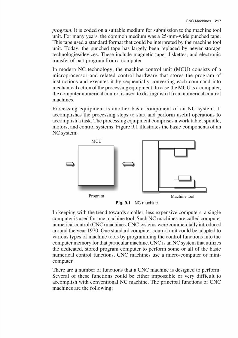
8/11/2019 Introduction to Mechatronics - Appuu Kuttan.pdf
http://slidepdf.com/reader/full/introduction-to-mechatronics-appuu-kuttanpdf 226/345
CNC Machines 217
program. It is coded on a suitable medium for submission to the machine toolunit. For many years, the common medium was a 25-mm-wide punched tape.This tape used a standard format that could be interpreted by the machine toolunit. Today, the punched tape has largely been replaced by newer storagetechnologies/devices. These include magnetic tape, diskettes, and electronic
transfer of part program from a computer.
In modern NC technology, the machine control unit (MCU) consists of amicroprocessor and related control hardware that stores the program ofinstructions and executes it by sequentially converting each command intomechanical action of the processing equipment. In case the MCU is a computer,the computer numerical control is used to distinguish it from numerical controlmachines.
Processing equipment is another basic component of an NC system. Itaccomplishes the processing steps to start and perform useful operations toaccomplish a task. The processing equipment comprises a work table, spindle,motors, and control systems. Figure 9.1 illustrates the basic components of anNC system.
Machine tool
MCU
Program
Fig. 9.1 NC machine
In keeping with the trend towards smaller, less expensive computers, a singlecomputer is used for one machine tool. Such NC machines are called computernumerical control (CNC) machines. CNC systems were commercially introducedaround the year 1970. One standard computer control unit could be adapted to
various types of machine tools by programming the control functions into thecomputer memory for that particular machine. CNC is an NC system that utilizesthe dedicated, stored program computer to perform some or all of the basicnumerical control functions. CNC machines use a micro-computer or mini-computer.
There are a number of functions that a CNC machine is designed to perform.Several of these functions could be either impossible or very difficult toaccomplish with conventional NC machine. The principal functions of CNCmachines are the following:
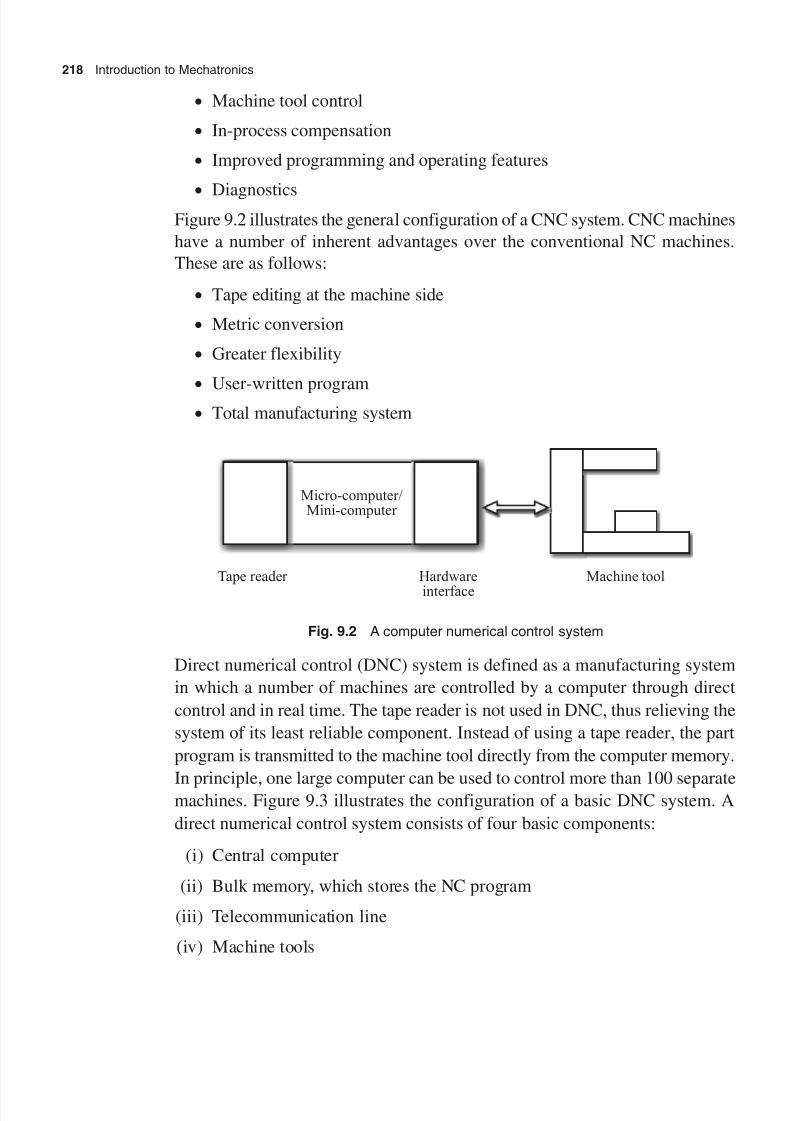
8/11/2019 Introduction to Mechatronics - Appuu Kuttan.pdf
http://slidepdf.com/reader/full/introduction-to-mechatronics-appuu-kuttanpdf 227/345
218 Introduction to Mechatronics
∑ Machine tool control
∑ In-process compensation
∑ Improved programming and operating features
∑ DiagnosticsFigure 9.2 illustrates the general configuration of a CNC system. CNC machines
have a number of inherent advantages over the conventional NC machines.
These are as follows:
∑ Tape editing at the machine side
∑ Metric conversion
∑ Greater flexibility
∑User-written program
∑ Total manufacturing system
Micro-computer/Mini-computer
Tape reader Hardware
interface
Machine tool
Fig. 9.2 A computer numerical control system
Direct numerical control (DNC) system is defined as a manufacturing system
in which a number of machines are controlled by a computer through direct
control and in real time. The tape reader is not used in DNC, thus relieving the
system of its least reliable component. Instead of using a tape reader, the part
program is transmitted to the machine tool directly from the computer memory.
In principle, one large computer can be used to control more than 100 separatemachines. Figure 9.3 illustrates the configuration of a basic DNC system. A
direct numerical control system consists of four basic components:
(i) Central computer
(ii) Bulk memory, which stores the NC program
(iii) Telecommunication line
(iv) Machine tools

8/11/2019 Introduction to Mechatronics - Appuu Kuttan.pdf
http://slidepdf.com/reader/full/introduction-to-mechatronics-appuu-kuttanpdf 228/345
CNC Machines 219
Fig. 9.3 Direct numerical control machine
There are several functions which a DNC system is designed to perform. These
functions are unique to DNC and could not be accomplished with either CNC
or conventional NC system. The principal functions of DNC are as follows:
∑ NC without punched tape
∑ NC part program storage
∑ Data collection, processing, and reporting
∑ Communication
Just as a CNC machine has certain advantages over a conventional NC system,
there are also advantages associated with the use of DNC. These are as follows:
∑ Elimination of punched tapes and tape reader
∑ Creation of computational capability and flexibility
∑ Convenient storage of part programs in computer files
∑ Program can be stored as a label
∑ Reporting of shop performance
∑ Provides the framework for the evolution of the future computer automated
factory
The combination of DNC and CNC provides the opportunity to add new
capabilities and refine existing ones in computerized manufacturing systems.
The DNC computer downloads the program directly to the CNC computer
memory. A second advantage created by combining CNC with DNC is redundancy.
If the central DNC computer fails, this will not necessarily cause the individual
8/11/2019 Introduction to Mechatronics - Appuu Kuttan.pdf
http://slidepdf.com/reader/full/introduction-to-mechatronics-appuu-kuttanpdf 229/345
220 Introduction to Mechatronics
machines in the systems to shut down. It is possible to provide the necessary
back-up to permit the CNC machines to operate on a stand-alone basis. There
are costs associated with providing the back-up features. A third advantage
from combined DNC and CNC systems is the improved communication between
the central computer and shop floor.
9.1 Adaptive Control Machine System
Adaptive control (AC) machining originated out of research in the early 1960s
and was sponsored by the US Air Force at the Bendix Research Laboratory for
machining operation. The term ‘adaptive control’ denotes a control system that
measures certain output process variables and uses this information to control
speed and/or feed. Some of the process variables that have been used in adaptive
control machining systems include spindle deflection, force, torque, cutting torque,
vibration amplitude, and horse power consumed. The motivation for developing
an adaptive machining system lies in trying to operate a process more efficiently.
Adaptive control is not appropriate for every machining situation. In general,
the following characteristics can be used to identify situations where adaptive
control can be beneficially applied:
(a) The in-process timing consumes a significant portion of machining cycle
time.
(b) There are significant sources of variability in the job for which adaptivecontrol can compensate.
(c) The cost of operating the machine tool is high.
(d) The typical jobs are those involving steel, titanium, and high strength alloys.
In the development of AC machining systems, two distinct approaches to the
problem can be used. These are
(i) AC optimization (ACO)
(ii) AC constraints (ACC)
In ACO, an index of performance is specified for the system. This performance
index is a measure of the overall process performance such as the production
rate or cost per unit volume of metal removed. Most of ACO systems attempt to
maximize the rate of work material removal to the tool wear rate. The index of
performance is a function of the material removal rate divided by the total wear
rate. The trouble with this performance index is that the tool wear rate cannot
be measured online with the current measurement technology.

8/11/2019 Introduction to Mechatronics - Appuu Kuttan.pdf
http://slidepdf.com/reader/full/introduction-to-mechatronics-appuu-kuttanpdf 230/345
CNC Machines 221
The systems developed for actual production are somewhat less sophisticated
than the research ACO system. The production AC systems utilize constraintlimits imposed on certain measured process variables. These are called adaptive
control constraint (ACC) systems.
9.2 CNC Machine Operations
Several modes of operation are usually available in NC systems. The auto mode
is the normal mode of operation. Other than the auto mode, NC systems may
use the manual or dial-in mode, the jogging mode, or the block-by-block mode.
The auto mode permits full automatic operation of the CNC, i.e., it allows
continuous execution of the part program. The manual data mode permits the
operator to dial in information to the control and thus instructs the machine to
follow the machine cycle without the use of a punched tape or stored program.
This is useful when setting up soft keys and is used to select information such as
spindle speeds, feeds, etc. and a button is used to transfer this information into
the control, one block at a time. The cycle start button is used to execute each
block of information. For set-up purposes, it is useful in controlling the slide
movements. Jogging switches permit this by selecting the direction and
appropriate axis and then pressing a button to move the slide. This mode is used
for coarse positioning. Fine positioning is carried out by discrete jogging
switches. Discrete jogging switches permit the axis to be moved by a known
distance, usually by 0.1, 0.01, or 0.001 mm. The axis and the increment of
movement are selected and the slides move at the press of a button. These
features can be used in setting up and in selecting the depth of a cut. In the
block-by-block mode with the tape in position, it is possible for the control to
read and execute one block’s information at a time. Successive press of the
cycle start button permits further blocks of the part program to read and execute
block by block.
9.2.1 Compensation and Override
Compensation and feed rate correlation are available in CNC control. Toolcompensation is very useful feature in control system and ensures thatprogramming is independent of the tool dimensions. The control system containsa memory in which both the tool length and radius compensation are stored.The tool zero offset or cutter radius compensation features are useful in millingapplications, where re-sharpened cutters or cutters of different diameters thanthe program size can be used without altering the tape. Roughing and finishingcuts can be made from the same tape and modifications to programmed
dimensions may also be made. Tool zero offsets are frequently added to lathe

8/11/2019 Introduction to Mechatronics - Appuu Kuttan.pdf
http://slidepdf.com/reader/full/introduction-to-mechatronics-appuu-kuttanpdf 231/345
222 Introduction to Mechatronics
controls to compensate for tool wear and to allow different diameters to be
machined in order to match the mating parts.
Tool features are similar to tool zero offset, but are applied to the spindle axis
only. These are particularly useful in drilling applications, where the varying
lengths of drills can be compensated. Feed rate override is often advantageousto the programmed feed rate, especially in cases where adverse cutting conditions
are encountered. If the program feed rates are unsuitable, it can be adjusted by
a dial usually calibrated in terms of the percentage of the program feed rate; 0
percent to 100 percent is most commonly used.
The sequence number read-out displays each block of information and has a
sequence number, for example N23, which means twenty-third block. It is
convenient to have the sequence number displayed so that the operator knows
which block of the program is being read at a particular time. This facility is
very useful when checking tapes or programs as it enables the operator to know
the location of any tape error.
The present position read-out display enables the operator to see on electronic
displays the present position of one or all axes. This is particularly useful when
the machine is being used manually and also when setting up the NC machine.
The CNC controller includes a keyboard for program or tape editing and a
cathode ray tube, on which messages are displayed or tool path can be displayed
for the operator. The machine tool consists of a work table, spindle, motors, and
machine control. It also includes cutting tools, work fixtures, and other auxiliaryequipment needed in the machining operation.
9.2.2 Co-ordinate System
A co-ordinate system consists of three mutually perpendicular axes intersecting
at a single point called the zero point. The three axes of the co-ordinate system
( X , Y , Z ) are used to identify the three planes, namely, the XY plane, YZ plane,
and ZX plane. Any plane located parallel to one of the planes is called a main
plane. A co-ordinate system aids in the location of points in the working zoneof a machine. There are two types of co-ordinate systems that are employed by
a control system to position the operation tool in relation to the work piece. The
Cartesian co-ordinates give paradoxical distance from one point to another.
The polar co-ordinates describe the position of a feature by a length measured
from a specified point and the angle measured in degrees from a specified datum
or reference axis. Most CNC machines operate only in linear dimensions. Only
special machining operation requires dimensional information. A second need
may be the ability to rotate a feature about a specified location.
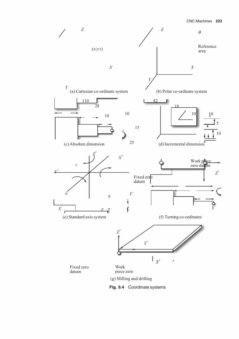
8/11/2019 Introduction to Mechatronics - Appuu Kuttan.pdf
http://slidepdf.com/reader/full/introduction-to-mechatronics-appuu-kuttanpdf 232/345
CNC Machines 223
( / / ) x y z
Z
X
Y (a) Cartesian co-ordinate system
Z
Y
X
Referencearea
(b) Polar co-ordinate system
(d) Incremental dimension
82
18
1010
10
5
28
10
15
25(c) Absolute dimension
110
10
Z +
X +
Y +
c
ab
Y –
X –
Z Z –
(e) Standard axis system
Fixed zerodatum
(f) Turning co-ordinates
X –
Work piecezero datum
Z +
Work piece zero
Fixed zerodatum
(g) Milling and drilling
Y +
Z +
X +
Fig. 9.4 Coordinate systems
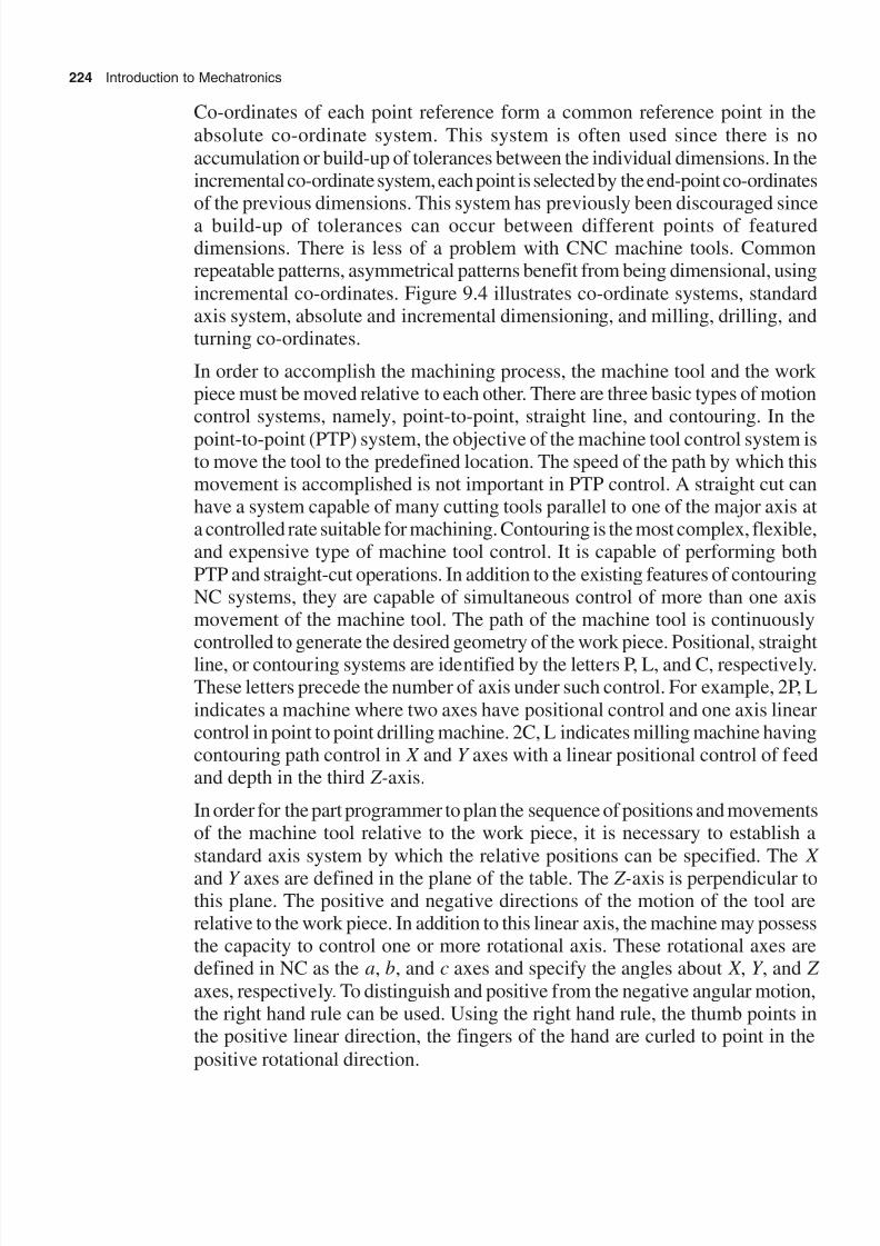
8/11/2019 Introduction to Mechatronics - Appuu Kuttan.pdf
http://slidepdf.com/reader/full/introduction-to-mechatronics-appuu-kuttanpdf 233/345
224 Introduction to Mechatronics
Co-ordinates of each point reference form a common reference point in theabsolute co-ordinate system. This system is often used since there is noaccumulation or build-up of tolerances between the individual dimensions. In theincremental co-ordinate system, each point is selected by the end-point co-ordinatesof the previous dimensions. This system has previously been discouraged sincea build-up of tolerances can occur between different points of featureddimensions. There is less of a problem with CNC machine tools. Commonrepeatable patterns, asymmetrical patterns benefit from being dimensional, usingincremental co-ordinates. Figure 9.4 illustrates co-ordinate systems, standardaxis system, absolute and incremental dimensioning, and milling, drilling, andturning co-ordinates.
In order to accomplish the machining process, the machine tool and the work piece must be moved relative to each other. There are three basic types of motioncontrol systems, namely, point-to-point, straight line, and contouring. In the
point-to-point (PTP) system, the objective of the machine tool control system isto move the tool to the predefined location. The speed of the path by which thismovement is accomplished is not important in PTP control. A straight cut canhave a system capable of many cutting tools parallel to one of the major axis ata controlled rate suitable for machining. Contouring is the most complex, flexible,and expensive type of machine tool control. It is capable of performing bothPTP and straight-cut operations. In addition to the existing features of contouringNC systems, they are capable of simultaneous control of more than one axismovement of the machine tool. The path of the machine tool is continuouslycontrolled to generate the desired geometry of the work piece. Positional, straightline, or contouring systems are identified by the letters P, L, and C, respectively.These letters precede the number of axis under such control. For example, 2P, Lindicates a machine where two axes have positional control and one axis linearcontrol in point to point drilling machine. 2C, L indicates milling machine havingcontouring path control in X and Y axes with a linear positional control of feedand depth in the third Z-axis.
In order for the part programmer to plan the sequence of positions and movementsof the machine tool relative to the work piece, it is necessary to establish astandard axis system by which the relative positions can be specified. The X
and Y axes are defined in the plane of the table. The Z-axis is perpendicular tothis plane. The positive and negative directions of the motion of the tool arerelative to the work piece. In addition to this linear axis, the machine may possessthe capacity to control one or more rotational axis. These rotational axes aredefined in NC as the a, b, and c axes and specify the angles about X , Y , and Zaxes, respectively. To distinguish and positive from the negative angular motion,the right hand rule can be used. Using the right hand rule, the thumb points inthe positive linear direction, the fingers of the hand are curled to point in thepositive rotational direction.

8/11/2019 Introduction to Mechatronics - Appuu Kuttan.pdf
http://slidepdf.com/reader/full/introduction-to-mechatronics-appuu-kuttanpdf 234/345
CNC Machines 225
For a turning operation, two axes are normally all that are required to command
the movement of the machine tool relative to the rotating work piece. The
Z -axis is the axis of rotation of the work piece and the X -axis defines the radial
location of the machine tool. The positive Z is the movement away from the
work piece and positive X is to increase the radius.
The work piece datum may be defined as the point, line, or surface from which
dimensions are referred. The machine datum is an established position within
the programmable area of the movement of the machine about which the machine
makes its programmed dimensional moves. It is often termed the zero datum or
simply zero. Each axis of the movement on the machine must have an established
zero datum point. This point may be fixed by the machine tool manufacturer or
may be defined by the user and set by the operator. It follows that the machine
datum must be referenced in some way to the work piece datum. Its locationwill depend on where the component is mounted. Machine datum facilities
generally take three forms, namely, fixed zero, zero offset, and datum shift and
floating zero. Fixed zero refers to an absolute fixed point on the machine. The
machine zero datum is fixed and cannot be repositioned by the operator. When
a machine utilizes this datum type, an important principle known as single
co-ordinate positioning is established. This means that all programmable
dimensions are assumed to be positive in sign from the fixed zero. This simplifies
the job of the part programmer. With this system, all programmed moves must
be made relative to the fixed datum of the machine. The machine operator needsto fix the component on the table in the specified position accurately, which is
more difficult. The zero offset facility allows the zero point to be specified to
any desired position within the programmable area of movement. Datum shift
permits the convenient location of the work piece on the machine work table,
since the machine zero can now be made to correspond with the work piece
datum. Part programming is simplified, since the component can be positioned
on the work table as per the convenience of the machine tool operator. The
floating zero or full floating zero is the most common datum system in operation.Any co-ordinate position may be described in terms of positive or negative
dimensions.
9.2.3 CNC Programming Procedure
The part programming often involves carrying out the task of process planning.
Process planning is the procedure of deciding what operations are to be done on
the component, in what order, and with what tool and work holding facilities.
8/11/2019 Introduction to Mechatronics - Appuu Kuttan.pdf
http://slidepdf.com/reader/full/introduction-to-mechatronics-appuu-kuttanpdf 235/345
226 Introduction to Mechatronics
Both part programming and process planning aspects of manufacture occur after
the detailed drawings of the component have been finalized. A part programmer
should be able to do the following:
∑ Plan work holding
∑ Plan operation sequence
∑ Decide on tooling
∑ Tabulate co-ordinate dimensions
∑ Ascertain part program format
∑ Code the part program
∑ Check, review, and modify the part program
∑ Formulate documentation
The necessary data for producing a part may come from the following:
∑ Information taken directly from the drawing
∑ Machining parameters
∑ Data determined by the part programming
∑ Information depending on particular NC system
There are two methods of part programming: manual part programming and
computer-assisted programming. In manual part programming, the program is
developed by means of NC codes; in computer-assisted programming, the
program is written in a higher language and the part program containing NC
codes is generated by the computer. Basically, there are two types of format:
∑ Fixed-block format
∑ Word-address format
In the fixed-block format, instructions contain all words in the same sequence
irrespective of the words being the same in the previous block. In each instruction,words are in the same sequence, but each word is preceded by a tab character. If
the instructions remain unchanged in the succeeding block, the instructions
need not be repeated, but the tab character must be punched in. In both the
cases, the identifying letter address need not be enlarged. Presently, the fixed-
block format is not used, since punched tapes are already obsolete.
In the word-address format, each word is preceded and identified by its letter
address. This format enables instructions that remain unchanged from the
8/11/2019 Introduction to Mechatronics - Appuu Kuttan.pdf
http://slidepdf.com/reader/full/introduction-to-mechatronics-appuu-kuttanpdf 236/345
CNC Machines 227
preceding blocks. This system speeds up programming and the length of tapes
is considerably reduced. This format is adopted by most of the CNC machine
control units.
A block is a group of words containing coded instructions for the NC system to
execute at a particular movement. Each block is separated from the next blockby an end of block (EOB) character. Each word consists of a letter and some
number. An example of a block follows:
N0090 G01 X150 Y270 Z-10 F10 S55 T01 D01 M08 EOB
where N0090 is a sequence number or line number, which is used to identify
the block. N0090 is called a word, N is the address and 0090 is a numerical
value. G01 is a preparatory function, X150 is the geometric X -axis instruction,
Y270 is the Y -axis instruction, Z 10 is the Z -axis instruction, F10 is the feed rate
instruction, S55 is the spindle speed in the structure, T01 is tool instruction,
D01 is the length compensation instruction, and M08 is the miscellaneous
instruction.
A preparatory function is a word used to prepare the controller for instructions.
Some preparatory function codes are as follows:
G00 Point-to-point positioning
G01 Linear interpolation
G02 Circular interpolation—clockwise
G03 Circular interpolation—anticlockwise
G04 Dwell
G05 Hold
G06 Parabolic interpolation
G08 Acceleration of the feed rate
G09 Deceleration of the feed rate
G10 Linear interpolation similar to G01 except that all dimensions
are multiplied by 10(used for incremental dimension)
G11 Linear interpolation similar to G01 except that all dimensions
are divided by 10
G13–G16 Used for axis selection for direct control system to operate in a
specific axis
G17 XY plane selection
8/11/2019 Introduction to Mechatronics - Appuu Kuttan.pdf
http://slidepdf.com/reader/full/introduction-to-mechatronics-appuu-kuttanpdf 237/345
228 Introduction to Mechatronics
G18 ZX plane selection
G19 YZ plane selection
G20 Circular interpolation in clockwise direction for long dimension
G21 Circular interpolation in clockwise direction for short dimension
G30 Circular interpolation in counterclockwise direction for long
dimension
G31 Circular interpolation in counterclockwise direction for short
dimension
G33 Thread cutting for constant lead
G34 Thread cutting for increasing lead
G35 Thread cutting for decreasing lead
G40 Cutter compensation cancel
G41 Cutter compensation left
G42 Cutter compensation right
G43–G49 Cutter compensation to adjust for difference between actual and
programmed cutter radius.
G60–G70 Reserved for positioning for part to part system
G80–G89 A fixed cycle or canned cycle while direct the machine to complete
such actionG90 Absolute dimension programming
G91 Incremental dimension programming
Co-ordinates specify the position for the tool. X , Y , and Z are used for the
primary motion of the tool and U , V , and W for the secondary motion. a, b, and
c specify angular dimensions and I , J , and K specify circular dimensions used
for thread cutting.
The F and S functions are used to specify the feed in a machining operation and
spindle rotation or cutting speed in RPM respectively. Tool function T is a word
needed only for machines with a tool turret or automatic tool changer. The
word T specifies which tool is to be used in the operation. The word D is used
to activate the cutter radius or length compensation. D0 is used to cancel the
tool length offset. The miscellaneous word M is used to specify certain
miscellaneous or auxiliary functions which may be available on the machine
tool such as coolant on/off, spindle/off, etc. The M function is also known as an
auxiliary function. Some standard machine functions are given below:
8/11/2019 Introduction to Mechatronics - Appuu Kuttan.pdf
http://slidepdf.com/reader/full/introduction-to-mechatronics-appuu-kuttanpdf 238/345
CNC Machines 229
M00 Program stop, which stops spindle coolant feed command.
M01 Optional stop, which is similar to M00 but it is performed only when
the operator has previously pushed a button.
M02 End of the program, which indicates the completion of all the
instructions.
M03 Starts spindle rotation in clockwise direction.
M04 Starts spindle rotation in counterclockwise direction.
M05 Stops the spindle and coolant.
M06 Executes the change of tool manually not to include tool selection.
M07 Turns flood coolant on.
M08 Turns mist coolant on.
M09 Automatically shuts the coolant off.
M10 Automatically clamps the slides, work piece, fixtures, spindle, etc.
M11 Unclamp command.
M13 Spindle rotates clockwise and coolant turns on.
M14 Spindle rotates counterclockwise and coolant turns on.
M15 Rapid transverse or feed rotate '+'.
M16 Motion enters + or – direction.
M19 The spindle to stop a predetermined angular position.
M30 End of tape similar to M02 except that rewinding tape or stop. This
makes ready for the next work piece.
M31 Interlock by pass which temporarily releases the normal interlock.
M32–M35 The control maintains a constant cutting speed by adjusting the rotation
of speed of work pieces.
M40–M45 Gear changers, if used, otherwise unassigned.
9.2.4 Interpolation
In contouring or continuous path systems, the tool is cutting while the axes of
motion are many. All axes of motion might move simultaneously, each at a
different velocity. When a non-linear path is required, the axial velocity changes

8/11/2019 Introduction to Mechatronics - Appuu Kuttan.pdf
http://slidepdf.com/reader/full/introduction-to-mechatronics-appuu-kuttanpdf 239/345
230 Introduction to Mechatronics
even within the segment, so the position of the cutting tool at the end of each
segment and the ratio between the axial velocities determine the desired contour
of the part. The system must contain a continuous position control loop in addition
to velocity controls. Dimensional information is given for each axis and is fed
through the data processing unit. The programmed feed rate of the contour,however, has to be processed by the control process unit (CPU) in order to
provide the proper velocity commands for each axis. This is done by means of
an interpolation which is contained in the CPU of the contouring system. The
function of the interpolator is to obtain intermediate points lying between those
taken from the drawing. In NC or CNC systems, three types of interpolators
exist—linear, circular, and parabolic. The most commonly used ones are linear
and circular.
For linear interpolation, G01 is used, which gives the displacement in straight
to the point where co-ordinates have been given in the same block. The same
goes for points in the subsequent blocks so long as G01 is not replaced by a
preparatory function of the same group. This displacement is at the programmed
feed rate and, therefore, fit for machining.
The function G02 or G03 is used to predict the displacement of the tool delay
circular arc. In G03 the tool movement is counterclockwise, while G02 has
clockwise movement. After G02 or G03, the coordinates X , Y , and Z of the end
position of the arc are programmed. The coordinates of the centre of the arc are
programmed with i, j, and k . Instead of the co-ordinates of the centre, the arccan also be defined by programming the radius, R. Figure 9.5 illustrates the
interpolation commands.
G00
G01
(a) Linear interpolation

8/11/2019 Introduction to Mechatronics - Appuu Kuttan.pdf
http://slidepdf.com/reader/full/introduction-to-mechatronics-appuu-kuttanpdf 240/345
CNC Machines 231
G02
E
C
A
Z +
E
C i = +
k = –
i = +
k = 0
A = Start pointE = End point
O = Center point
k = –
Z +
(b) Circular interpolation clockwise
E
C
A
C
E
A
G03
(c) Circular interpolation counterclockwise
i = –
k = –
i = 0
k = –
Fig. 9.5 Interpolation
9.2.5 Cutter Compensation
The important consideration in programming is to program the required path
with respect to the centre of the tool considering a nominal radius value ratherthan at the point on its periphery where actual cutting takes place. The differencebetween the programmed radius and the actual radius of the cutter tools can beeasily accommodated using the cutting radius compensation facility. The cutterradius compensation value is entered into the control unit adjacent to each toolnumber. Cutter compensation is defined as the correlation normal to a controlledaxis. When cutter compensation is provided, the control unit generates a newtool path which is equidistant from the programmed cutter path by the differencebetween the programmed radius and the actual radius of the cutter. This is thecompensator dimension. It is necessary to indicate whether these corrections

8/11/2019 Introduction to Mechatronics - Appuu Kuttan.pdf
http://slidepdf.com/reader/full/introduction-to-mechatronics-appuu-kuttanpdf 241/345
232 Introduction to Mechatronics
are to take place to the right or to the left of the tool. By G41, the compensationis applied to shift the program path to the left. By G42, the compensation isapplied to shift the program path to the right. Left and right are identified byassuming a point on the top face of the tool focusing the direction of the cut.G40 is used to cancel the cutter radius compensation.
The tool offset is defined as a correlation parallel to a control axis. In the case ofthe CNC milling machine such correlation is required to take care of thedifference between the programmed length of a cutter and its actual length.Such an offset is known as the tool length offset. When using a single tool, it iscommon practice to set the tool down manually to the reference plane and setthis position to be Z00 or the tool may be set down to touch the surface of thework and then retracted by the desired amount, by referencing the Z -axis displayon the operator console. When using a single tool, the tool length offset is zero.When a second tool is used or the original tool is replaced with the some partprogram, there will be certain differences in length from that of the originaltool. This will result in an error if used directly. To account for such discrepancies,the difference in length between the first tool and subsequent tools is noted andstored as a tool length offset within the memory of the control unit. When adifferent tool is called for use, either T or D word is used. Its corresponding toolcarries the offset and causes the programmed Z -axis position to be modified bythe specified amount. One can use T0 or D00 to cancel the tool length offset.Figure 9.6 shows the cutter length compensation and cutter radius compensation.
Fig. 9.6 Cutter compensation
An optional stop facility is available in some control systems in which some ofthe unwanted program blocks can be temporarily stopped while running aprogram by inserting ‘l’ or ‘m’ word before the start of the program block. Theblock in question will not be deleted from the program and if that block is to beexecuted again, it can be done just by erasing the character.

8/11/2019 Introduction to Mechatronics - Appuu Kuttan.pdf
http://slidepdf.com/reader/full/introduction-to-mechatronics-appuu-kuttanpdf 242/345
CNC Machines 233
9.2.6 Part Program
A part program defines a sequence of NC machine operations. The informationcontained in the program can be dimensional or non-dimensional such as speed,feed, auxiliary functions, etc. The basic unit of a part program input to the control
is called a block. Each block contains adequate information for the machine toperform a movement and/or a function. All blocks are terminated by the blockend character,*. The maximum block length in each NC machine is fixed.
In the absolute dimensioning, all the dimensions are measured in the samedirection from a fixed datum. In incremental dimensioning, adjacent dimensionsare placed in series in a row or column. The disadvantage of incrementaldimensioning method is that the tolerance on each dimension is accumulated.The following examples illustrate the part programming for absolute andincremental dimensional work pieces.
Figure 9.7 shows a part drawing. It requires X and Y axes to position first onpoint 1 and then to points 2, 3, and 4, with co-ordinates (100, 100), (150,125),(200,150), and (250, 175), respectively, from the datum.
3
2
1
4
N5 G71 *_ ---- metric N10 G90 *_ ---- absdnle N15 G00 X100 Y100 * N20 X150 Y175 * N25 X200 Y125 *
N30 X250 Y150 * Fixed datum
Fig. 9.7 Absolute program
The part drawing shown in Fig. 9.8 requires programmable X and Y axes toposition from first point 1, point 2, and point 3, for which the incremental pointsin the X -direction are 20, 50, and 100 and in the Y -direction are 40, 60, and 80.
The fixed datum is at (100, 100) from the edge of work piece.
3
2
1
N5 G71 * N10 G90 X100 Y100 * N15 G91 * N20 G00 X20 Y40 * N25 X50 Y60 * N30 X100 Y80 *
Fixed datum
Fig. 9.8 Incremental program
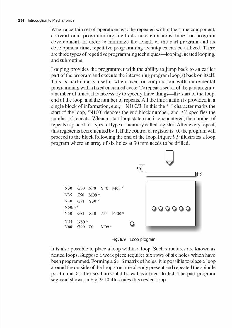
8/11/2019 Introduction to Mechatronics - Appuu Kuttan.pdf
http://slidepdf.com/reader/full/introduction-to-mechatronics-appuu-kuttanpdf 243/345
234 Introduction to Mechatronics
When a certain set of operations is to be repeated within the same component,conventional programming methods take enormous time for programdevelopment. In order to minimize the length of the part program and itsdevelopment time, repetitive programming techniques can be utilized. Thereare three types of repetitive programming techniques—looping, nested looping,and subroutine.
Looping provides the programmer with the ability to jump back to an earlierpart of the program and execute the intervening program loop(s) back on itself.This is particularly useful when used in conjunction with incrementalprogramming with a fixed or canned cycle. To repeat a sector of the part programa number of times, it is necessary to specify three things—the start of the loop,end of the loop, and the number of repeats. All the information is provided in a
single block of information, e.g., = N100/3. In this the ‘=’ character marks the
start of the loop, ‘N100’ denotes the end block number, and ‘/3’ specifies thenumber of repeats. When a start loop statement is encountered, the number ofrepeats is placed in a special type of memory called register. After every repeat,
this register is decremented by 1. If the control of register is ‘0, the program willproceed to the block following the end of the loop. Figure 9.9 illustrates a loopprogram where an array of six holes at 30 mm needs to be drilled.
5
50
N30 G00 X70 Y70
N35 Z50 M08 *
M03 *
N40 G91 Y30 *
N50/6 *
N50 G81 X30 Z55 F400 *
N80 * N55
N60 G90 Z0 M09 *
Fig. 9.9 Loop program
It is also possible to place a loop within a loop. Such structures are known asnested loops. Suppose a work piece requires six rows of six holes which havebeen programmed. Forming a 6 ¥ 6 matrix of holes, it is possible to place a looparound the outside of the loop structure already present and repeated the spindleposition at Y , after six horizontal holes have been drilled. The part programsegment shown in Fig. 9.10 illustrates this nested loop.
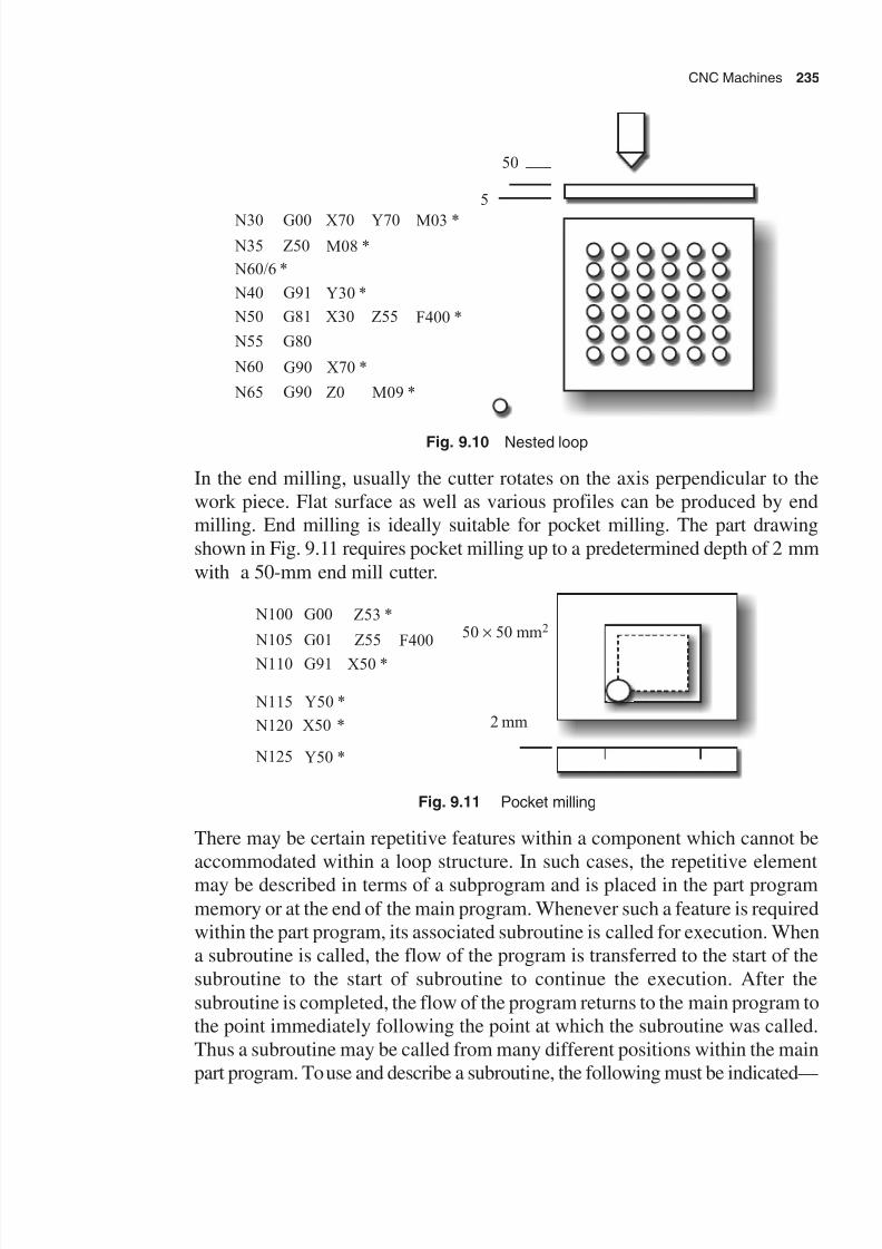
8/11/2019 Introduction to Mechatronics - Appuu Kuttan.pdf
http://slidepdf.com/reader/full/introduction-to-mechatronics-appuu-kuttanpdf 244/345
CNC Machines 235
50
5
N30 G00 X70 Y70
N35 Z50 M08 *
M03 *
N40 G91 Y30 *
N60/6 *
N50 G81 X30 Z55 F400 *
G90 N60
N65 G90 Z0 M09 *
N55 G80
X70 *
Fig. 9.10 Nested loop
In the end milling, usually the cutter rotates on the axis perpendicular to thework piece. Flat surface as well as various profiles can be produced by endmilling. End milling is ideally suitable for pocket milling. The part drawingshown in Fig. 9.11 requires pocket milling up to a predetermined depth of 2 mmwith a 50-mm end mill cutter.
2 mm
N100 G00
N105 G01 F400
Z53 *
N110 G91 X50 *
N115
N120 X50 *
Y50 * N125
Z55
Y50 *
50 50 mm 2
Fig. 9.11 Pocket milling
There may be certain repetitive features within a component which cannot beaccommodated within a loop structure. In such cases, the repetitive elementmay be described in terms of a subprogram and is placed in the part program
memory or at the end of the main program. Whenever such a feature is requiredwithin the part program, its associated subroutine is called for execution. Whena subroutine is called, the flow of the program is transferred to the start of thesubroutine to the start of subroutine to continue the execution. After thesubroutine is completed, the flow of the program returns to the main program tothe point immediately following the point at which the subroutine was called.Thus a subroutine may be called from many different positions within the mainpart program. To use and describe a subroutine, the following must be indicated—

8/11/2019 Introduction to Mechatronics - Appuu Kuttan.pdf
http://slidepdf.com/reader/full/introduction-to-mechatronics-appuu-kuttanpdf 245/345
236 Introduction to Mechatronics
the start of the subroutine and the end of the subroutine. For instance #3 or L3will indicate the start of the subroutine number 3.
The M word or $ character is used to indicate the end of the subroutine. Thesubroutine may be called from the main program by a calling line such as = #3,
which means call subroutine 3. The part drawing shown in Fig. 9.12 requirespocket milling of square profiles of 50 ¥ 50 mm2 at a depth of 2 mm at variouspositions in a flat plate component. The program follows as shown in Fig. 9.13.The starting point co-ordinates for pockets 1, 2, and 3 are (50, 150), (100, 100),
and (300, 160), respectively.
Main program
1
3
2
N1 G00 X0Y0Z0 *
N2 G00 Y150 *
N4 = #1 *
N4
#1 N7=
N8 G00 X0Y0Z0
X50
G00 X200 Y100
N5 = #1
N6 G00 X300 Y180
N9 M02
% 200
Fig. 9.12
Subroutine
50 50 mm 2
N100 G00 Z53 *
N105 G01 F400 *
N110
N115
G90 * N130
N135 G00 Z53 *
Z55
Y50 *
N120
N125 Y50 *
N140 $ *
#1
X50 *G91
X50 *
Fig. 9.13 Subroutine
A subroutine may be called after a subroutine. But subroutines must not bedefined within a subroutine. A macro is a single command that generates aseries of tool paths for the execution of a particular machining operation. Themacro call within the part program must invariably be accompanied by additionalinformation. Macros may be predefined as in-built control system facilities orthey may be user-defined. In the latter case, the implementation of a macro is

8/11/2019 Introduction to Mechatronics - Appuu Kuttan.pdf
http://slidepdf.com/reader/full/introduction-to-mechatronics-appuu-kuttanpdf 246/345
CNC Machines 237
similar to that of a subroutine. In fact, the terms ‘subroutine’ and ‘macro’ areused without distinction by some manufacturers.
A macro can be thought of as a subroutine with the ability to pass values orparameters. A parameter is a value that acts as a constant value in the process,
but may take different values from run to run. For example, the subroutinedescribed earlier will not mill a single square projectile of 50 ¥ 50 mm2 only. Itcannot mill a principle of any other dimension. With macro facilities, it will bepossible to mill the same principle with different dimensions by simply passingdifferent parameter values with the calling line. With macros, it is necessary tospecify parameters that may change from call to call, a means of passing truevalues into these parameters. Within the macro definition the parameter likelyto change is not given any numerical values, but is marked with an asterisk.True numerical values are supplied when the macro is called. Figure 9.14 showsa part drawing that requires pocket milling using macros. The starting pointco-ordinates for pockets 1, 2, and 3 are (50, 150), (100, 100), and (300, 160),respectively. The starting point co-ordinates for points 1 and 2 are at (100, 100)
and (200, 125), respectively.
1
2
N1 G00 X0Y0Z0 *
N2 G00 Y100 *
N3 = #1
N4
X100
G00
N7 M02
#Z01 *
X 50 Y X
X200 Y125
N5 = #1
Subroutine
N100 G00 Z53 *
N105 G01 Z55 F400 *
N110 G91
N115
N125
G90 N130
N135 G00 Z53
#1 *
X
Y
N120 XY
Main program
* * 50 * 50 Y* 50
100X * Y* 50 X* 100 Y* 50
*
*
**
*
*
Fig. 9.14 Use of macros
Many control systems offer additional features that aid the programming of
repetitive features. Most of these are invoked by G or M codes within the part
program. Some common features available on a milling machine are:

8/11/2019 Introduction to Mechatronics - Appuu Kuttan.pdf
http://slidepdf.com/reader/full/introduction-to-mechatronics-appuu-kuttanpdf 247/345
238 Introduction to Mechatronics
∑ reflection or mirror imaging
∑ scaling
∑ rotation
∑ translation
Many engineering components need to be produced in handed pairs, right handedparts and left handed parts. The two components are invariably identical in
dimensions but are geometrically opposite. For this purpose, the mirror imaging
facility is employed. The line along which the component is mirrored is known
as the axis symmetry. In the CNC control system, two axes’ reflections are
normally accommodated, reflections along X and Y axes. In this approach all X +
dimensions become X – = dimensions for reflection along the Y-axis and all Y +
dimensions become Y – dimensions for reflection along the X -axis. The control
system automatically arranges this on the receipt of the requisite G code within
the program. Three possibilities are available, reflection along X , reflectionalong Y , and reflection along both X and Y simultaneously. Reflection normally
occurs about the absolute programmed datum X0, Y0. Figure 9.15 shows the
part drawing required for engraving the letter ‘F’ and its mirror images.
20 30
35
30
2010
306
N1 G00 X0Y0Z0 *
– * N2 G17
N3 #3M84 * N4
N5 = #3
Main program
% Z0
– *
T1 M03 *
#3
M83 *
N9 = #3 M82 *
N7 M80 T0
N8 G00 M30
N100 G00 X20
N101 G01
N102 Y30
N103
Subroutine
#3
Z53 F100
X35
Y10 Z50 M08
N104 G00 Z50 N105 X20 Y20
N106 G01 Z53
N107 X30 N108 G00 Z50
N109 $
Fig. 9.15 Mirror imaging

8/11/2019 Introduction to Mechatronics - Appuu Kuttan.pdf
http://slidepdf.com/reader/full/introduction-to-mechatronics-appuu-kuttanpdf 248/345
CNC Machines 239
Many components consist of a single element which rotates about a specified
origin. The origin is normally the absolute X0, Y0. Common examples are
holes or slots on a common pitch circle diameter or components comprising
radial features such as arrows or spokes. If such a facility is specified using the
preparatory function G code, it must be accompanied by the informationspecifying the angle of rotation and the pole of rotation.
Translation is used to produce a series of identical features shifted by a specified
amount from the previous one. The shift may be in one or more axes. This can
be accomplished by utilizing the appropriate preparatory G code within the part
program and specifying the X and Y coordinates for the new starting point.
A scaling facility allows the cutter path to be transformed by increasing (scaling
up) or decreasing (scaling down) it. Its magnitudes are relative to its programmed
dimensions. The actual programmed dimensions are considered to have a scale
value of 1. When a scaling facility is involved, extra information is supplied
specifying the scaling required in the X and Y axes. A family of different-sized
components may thus be machined using a single part program. The effects of
rotation, translation, and scaling are illustrated in Fig. 9.16.
(a) (b)
(c)
Fig. 9.16 (a) Rotation, (b) translation, and (c) scaling canned cycles or fixed cycles
A canned or fixed cycle is a fixed sequence of operations, in-built in the controlsystem, which can be brought into action by a single command. Such cyclesconsiderably reduce the programming time and effort in repetitive and commonly
used machining operations. Preparatory function codes G81 to G89 are reserved
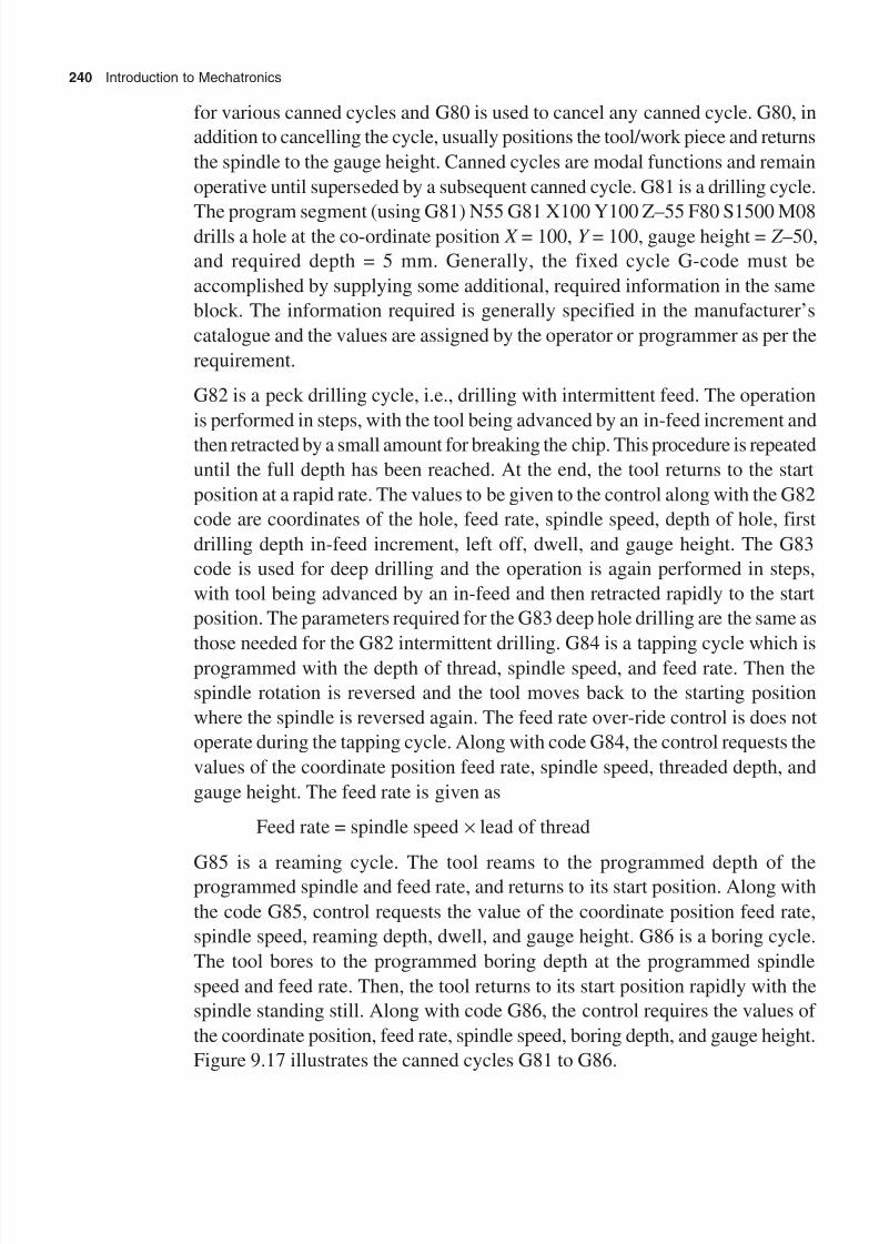
8/11/2019 Introduction to Mechatronics - Appuu Kuttan.pdf
http://slidepdf.com/reader/full/introduction-to-mechatronics-appuu-kuttanpdf 249/345
240 Introduction to Mechatronics
for various canned cycles and G80 is used to cancel any canned cycle. G80, in
addition to cancelling the cycle, usually positions the tool/work piece and returns
the spindle to the gauge height. Canned cycles are modal functions and remain
operative until superseded by a subsequent canned cycle. G81 is a drilling cycle.
The program segment (using G81) N55 G81 X100 Y100 Z–55 F80 S1500 M08drills a hole at the co-ordinate position X = 100, Y = 100, gauge height = Z –50,
and required depth = 5 mm. Generally, the fixed cycle G-code must be
accomplished by supplying some additional, required information in the same
block. The information required is generally specified in the manufacturer’s
catalogue and the values are assigned by the operator or programmer as per the
requirement.
G82 is a peck drilling cycle, i.e., drilling with intermittent feed. The operation
is performed in steps, with the tool being advanced by an in-feed increment and
then retracted by a small amount for breaking the chip. This procedure is repeated
until the full depth has been reached. At the end, the tool returns to the start
position at a rapid rate. The values to be given to the control along with the G82
code are coordinates of the hole, feed rate, spindle speed, depth of hole, first
drilling depth in-feed increment, left off, dwell, and gauge height. The G83
code is used for deep drilling and the operation is again performed in steps,
with tool being advanced by an in-feed and then retracted rapidly to the start
position. The parameters required for the G83 deep hole drilling are the same as
those needed for the G82 intermittent drilling. G84 is a tapping cycle which is
programmed with the depth of thread, spindle speed, and feed rate. Then the
spindle rotation is reversed and the tool moves back to the starting position
where the spindle is reversed again. The feed rate over-ride control is does not
operate during the tapping cycle. Along with code G84, the control requests the
values of the coordinate position feed rate, spindle speed, threaded depth, and
gauge height. The feed rate is given as
Feed rate = spindle speed ¥ lead of thread
G85 is a reaming cycle. The tool reams to the programmed depth of theprogrammed spindle and feed rate, and returns to its start position. Along with
the code G85, control requests the value of the coordinate position feed rate,
spindle speed, reaming depth, dwell, and gauge height. G86 is a boring cycle.
The tool bores to the programmed boring depth at the programmed spindle
speed and feed rate. Then, the tool returns to its start position rapidly with the
spindle standing still. Along with code G86, the control requires the values of
the coordinate position, feed rate, spindle speed, boring depth, and gauge height.
Figure 9.17 illustrates the canned cycles G81 to G86.
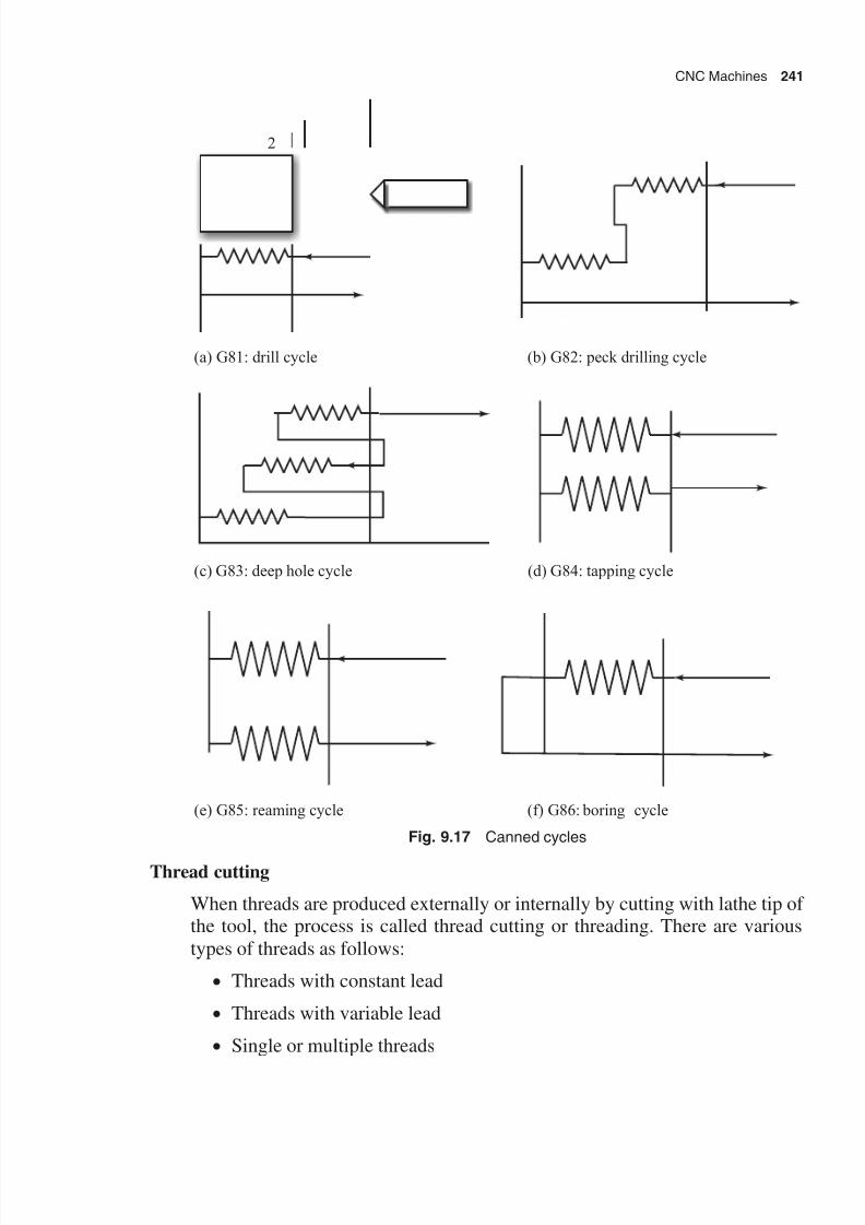
8/11/2019 Introduction to Mechatronics - Appuu Kuttan.pdf
http://slidepdf.com/reader/full/introduction-to-mechatronics-appuu-kuttanpdf 250/345
CNC Machines 241
(a) G81: drill cycle (b) G82: peck drilling cycle
(c) G83: deep hole cycle
2
(d) G84: tapping cycle
(e) G85: reaming cycle (f) G86: boring cycle
Fig. 9.17 Canned cycles
Thread cutting
When threads are produced externally or internally by cutting with lathe tip ofthe tool, the process is called thread cutting or threading. There are varioustypes of threads as follows:
∑ Threads with constant lead
∑ Threads with variable lead
∑ Single or multiple threads

8/11/2019 Introduction to Mechatronics - Appuu Kuttan.pdf
http://slidepdf.com/reader/full/introduction-to-mechatronics-appuu-kuttanpdf 251/345
242 Introduction to Mechatronics
∑ Threads on cylindrical or tapered surfaces
∑ External or internal threads
∑ Transverse threads
Preparatory function G33 is used to machine all types of threads with constantlead. The thread length is entered under the corresponding path address I, K.The lead is read under K for longitudinal threads and under ± for transversethreads. I and K values must always be entered using incremental position dataand without sign. The right- and left-hand threads are programmed by specifyingthe spindle direction of rotation functions M03 and M04. The spindle directionof rotation and spindle speed must be programmed in the block prior to theactual thread cutting operation to permit the spindle to run up to its nominalspeed. The feed rate, F, is not programmed here, since it is linked directly to thespindle speed via pulse encoder. The feed start does not begin until the zeromark is reached on the pulse encoder in order to permit the threads to be cut inseveral steps. This ensures that the tool always enters the work piece at thesame point on the circumference of the work piece. The cut should beimplemented at the same spindle speed override. The switch and single block mode switch have no effect during thread cutting. Figure 9.18 illustrates thethread on a cylindrical block and its program details.
P4
P3
P6
X +
P1
P2
P5
3 mm50 mm 3 mm
Lead, = 2 mmThread depth, – = 1.3 mmIn-feed direction is radial.
h
h t
Program
%10
N20 G90 S44*
N21 G00 X46 Z3*N22 X38.7*
N23 G33 Z53 K2*
N24 G00 X46*
N25 Z3 (P1)*
N26 X37.4 (P5)*
N27 G33 Z53 K2 (P6)*
N28 G00 X46 (P4)*
N29 M02*Fig. 9.18 Thread program: cylindrical thread

8/11/2019 Introduction to Mechatronics - Appuu Kuttan.pdf
http://slidepdf.com/reader/full/introduction-to-mechatronics-appuu-kuttanpdf 252/345
CNC Machines 243
Taper thread
Taper thread fastening is generally used for the extension of rotating shafts. The
advantage of taper thread is the quick removal of the assembly even if there is a
cold welding between the bolt and the nut. Figure 9.19 shows a thread on a
tapered block and its program details. In-feed direction is radial.
Lead h = 5 mm
Thread depth t = 1.73 mm
Angle a = 15 deg
Both the end position co-ordinates must be written.
The lead is entered under K.
Calculate thread start co-ordinates. A, B, C , etc. are diameters.
First cut P2 and P3: t = 1 mm
Second cut P5 and P6: t = 1.73 mm
A = 70, B = A – 2t = 66.54
C = B – 2 (5 tan 15°) = 63.86
D = C + Z (70 tan 15°) = 101.366
P4
P3
P6
P2
P5
5 60 5
X +
(a)
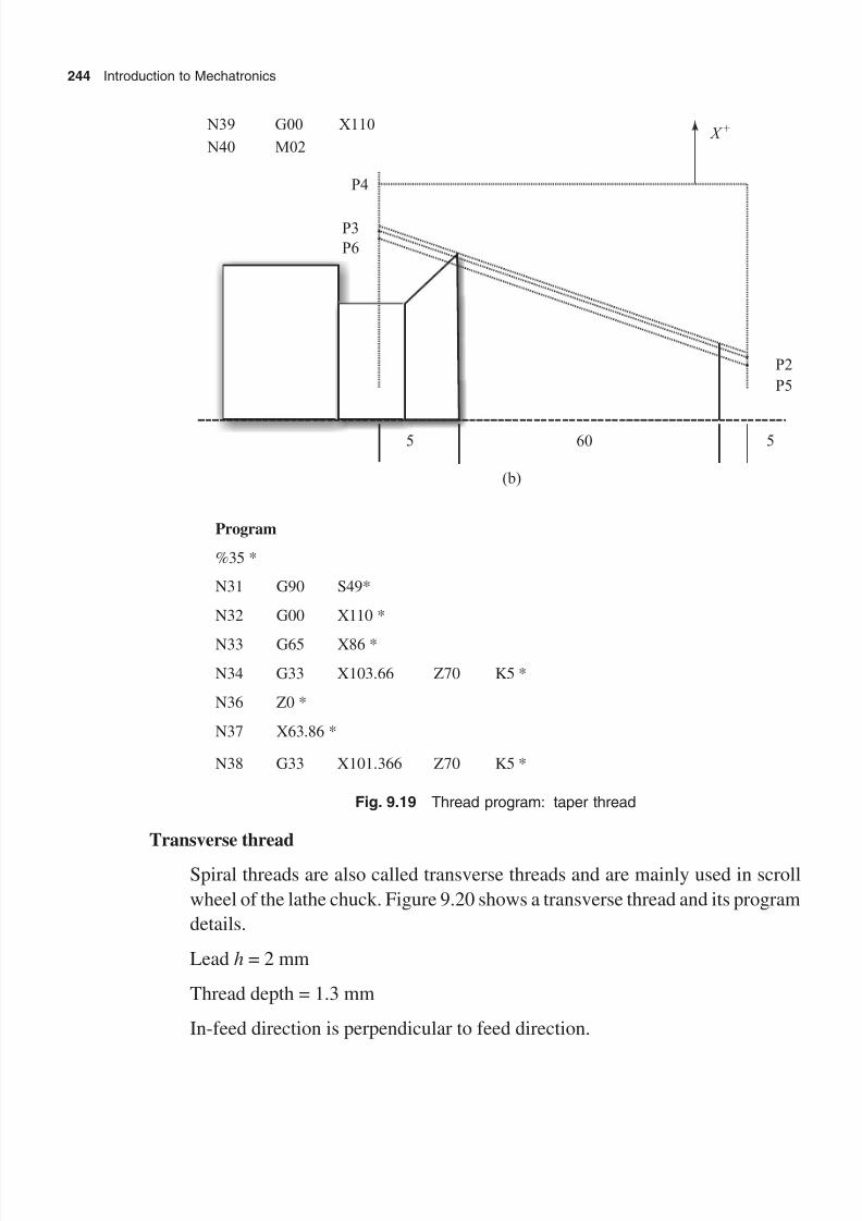
8/11/2019 Introduction to Mechatronics - Appuu Kuttan.pdf
http://slidepdf.com/reader/full/introduction-to-mechatronics-appuu-kuttanpdf 253/345
244 Introduction to Mechatronics
N39 G00 X110
N40 M02
P4
P3
P6
P2
P5
X +
5 60 5
(b)
Program
%35 *
N31 G90 S49*
N32 G00 X110 *
N33 G65 X86 *
N34 G33 X103.66 Z70 K5 *
N36 Z0 *
N37 X63.86 *
N38 G33 X101.366 Z70 K5 *
Fig. 9.19 Thread program: taper thread
Transverse thread
Spiral threads are also called transverse threads and are mainly used in scroll
wheel of the lathe chuck. Figure 9.20 shows a transverse thread and its program
details.
Lead h = 2 mm
Thread depth = 1.3 mm
In-feed direction is perpendicular to feed direction.
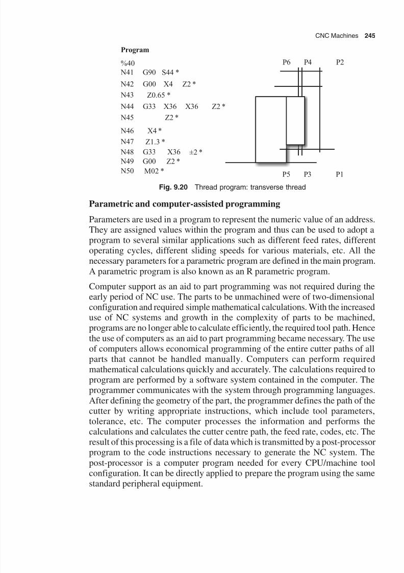
8/11/2019 Introduction to Mechatronics - Appuu Kuttan.pdf
http://slidepdf.com/reader/full/introduction-to-mechatronics-appuu-kuttanpdf 254/345
CNC Machines 245
P6 P4 P2
P5 P3 P1
N41 G90
N42 X4 Z2 *
S44 *
N43 Z0.65 *
N46
N47 Z1.3 *
±2 * N48
N49 G00 Z2 *
Program
%40
G00
N44 X36 Z2 *G33 X36
N45 Z2 *
G33
X4 *
X36
N50 M02 *
Fig. 9.20 Thread program: transverse thread
Parametric and computer-assisted programming
Parameters are used in a program to represent the numeric value of an address.They are assigned values within the program and thus can be used to adopt aprogram to several similar applications such as different feed rates, differentoperating cycles, different sliding speeds for various materials, etc. All thenecessary parameters for a parametric program are defined in the main program.A parametric program is also known as an R parametric program.
Computer support as an aid to part programming was not required during the
early period of NC use. The parts to be unmachined were of two-dimensionalconfiguration and required simple mathematical calculations. With the increaseduse of NC systems and growth in the complexity of parts to be machined,programs are no longer able to calculate efficiently, the required tool path. Hencethe use of computers as an aid to part programming became necessary. The useof computers allows economical programming of the entire cutter paths of allparts that cannot be handled manually. Computers can perform requiredmathematical calculations quickly and accurately. The calculations required toprogram are performed by a software system contained in the computer. Theprogrammer communicates with the system through programming languages.
After defining the geometry of the part, the programmer defines the path of thecutter by writing appropriate instructions, which include tool parameters,tolerance, etc. The computer processes the information and performs thecalculations and calculates the cutter centre path, the feed rate, codes, etc. Theresult of this processing is a file of data which is transmitted by a post-processorprogram to the code instructions necessary to generate the NC system. Thepost-processor is a computer program needed for every CPU/machine toolconfiguration. It can be directly applied to prepare the program using the samestandard peripheral equipment.

8/11/2019 Introduction to Mechatronics - Appuu Kuttan.pdf
http://slidepdf.com/reader/full/introduction-to-mechatronics-appuu-kuttanpdf 255/345
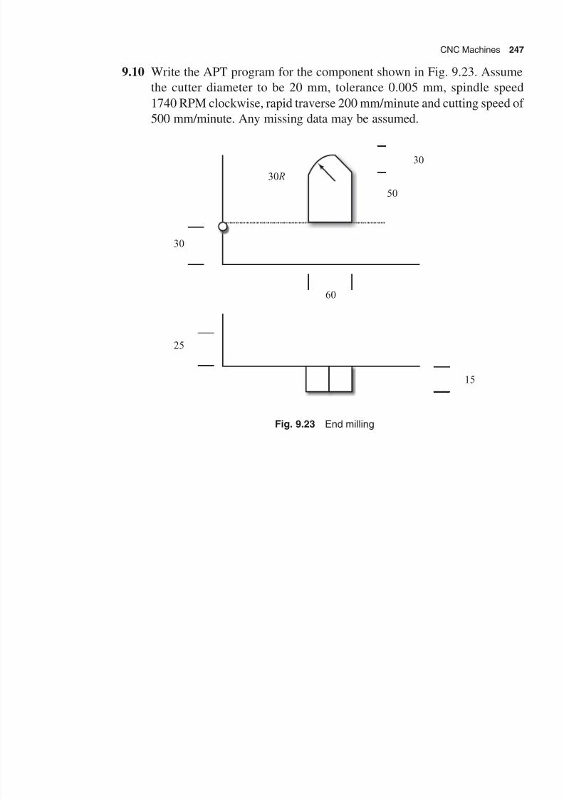
8/11/2019 Introduction to Mechatronics - Appuu Kuttan.pdf
http://slidepdf.com/reader/full/introduction-to-mechatronics-appuu-kuttanpdf 256/345
CNC Machines 247
9.10 Write the APT program for the component shown in Fig. 9.23. Assume
the cutter diameter to be 20 mm, tolerance 0.005 mm, spindle speed
1740 RPM clockwise, rapid traverse 200 mm/minute and cutting speed of
500 mm/minute. Any missing data may be assumed.
30 R
30
50
30
60
25
15
Fig. 9.23 End milling

8/11/2019 Introduction to Mechatronics - Appuu Kuttan.pdf
http://slidepdf.com/reader/full/introduction-to-mechatronics-appuu-kuttanpdf 257/345
8/11/2019 Introduction to Mechatronics - Appuu Kuttan.pdf
http://slidepdf.com/reader/full/introduction-to-mechatronics-appuu-kuttanpdf 258/345
Intelligent Systems and Their Applications 249
operators can control many processes successfully without using any quantities
modelling method. The control strategy of the human operator is based mainly on
linguistics and qualitative knowledge concerning the behaviour of an ill-defined
process. Most modelling processes are based on the nature of the system. Non-
linear and ill-defined processes can be easily controlled by fuzzy logic. The conceptsof neural system and fuzzy control link the idea of linguistic control and deterministic
decision making.
A recent technological advancement in mechatronic systems is the microsystem
engineering. Microsystem engineering involves the designing, manufacturing,
and packaging of micro-electro-mechanical systems (MEMS). The applications
of microsystems are in aerospace, automotive, biotechnology, consumer
products, environmental protection, safety health care, pharmaceuticals, and
telecommunication. Many industries promoted drug microsystems and related
products in the year 2000.
Nanoscience and nanotechnology are two hottest fields in science, business,
and news today. MEMS, nanoscience, and nanotechnology are subdomains of
mechatronics. Nanoscience, as the name suggests, is the study of fundamental
principles of molecules and structures with at least one dimension roughly
between one nanometre to hundreds of nanometres. Structures of this scale are
known as nanostructures. Nanotechnology is the application of nanostructures
in the useful nanoscale devices. Nanotechnology should not be confused with
MEMS. MEMS are concerned with structures between 1000 and 1000000nanometers, i.e., with structures much bigger than nanoscale structure. Nanoscience
and nanotechnology are concerned with all properties of structures of the nanoscale,
whether chemical, biological, or mechanical. Nanotechnology is more diverse and
stretches into dozens of subfields.
To function effectively and optimally, all the smart technology needs artificial
intelligence. Hence the tools used to incorporate artificial intelligence are equally
important. Some of the tools used for artificial intelligence are discussed in the
sections that follow.
10.1 Artificial Neural Network
An artificial neural network (ANN) is an information processing system acting
as a black box device that accepts input and produces output. In earlier days,
neural networks have been widely used for pattern recognition. In this case an
input pattern is passed to a network and the network produces a representative
class of output. The ANN has pattern matching, pattern completing, noise

8/11/2019 Introduction to Mechatronics - Appuu Kuttan.pdf
http://slidepdf.com/reader/full/introduction-to-mechatronics-appuu-kuttanpdf 259/345
250 Introduction to Mechatronics
removal, and controlling abilities to create a desired response. A neural network
consists of processing elements (PEs) and weighted connections. Figure 10.1
illustrates a typical neural network model. The first layer consists of a collection
of processing elements. Each PE in the neural network collects the values from
all its input connections to produce output values. The PEs are connected withweighted connections. The weighted connections are stored information. The value
of a connection weight is often determined by the neural network procedure. Some
important features of neural networks are as follows:
1. Each PE acts independently.
2. PEs rely only on local information.
3. A large number of connections provide a large amount of redundancy.
x x x, , 31 2
y y,1 2
Inputs Outputs
z z z , , 31 2
Fig. 10.1 Neural network model
The first two features allow the neural networks to operate efficiently in parallel.
The third feature provides for generalization of the state of qualities, which is
very difficult in a typical computing system. In addition to the introduction of
non-linearity in the PE, an ANN arbitrarily learns non-linear mapping by
appropriate learning rules. Major advantages of neural network are as follows:
1. A few decisions are required from among massive amount of data.
2. A non-linear mapping is required automatically.
3. An optimal solution to the problem is obtained very quickly.
A neural network consists of three principal elements, namely, topology, learning,
and recall. Topology indicates how a neural network is organized into layers.
Learning describes how the information is stored in the neural network. And
recall means retrieving the stored information when required.
8/11/2019 Introduction to Mechatronics - Appuu Kuttan.pdf
http://slidepdf.com/reader/full/introduction-to-mechatronics-appuu-kuttanpdf 260/345
Intelligent Systems and Their Applications 251
The following conventions, created in 1990, are used for ANNs. The input and
output vectors are denoted by a capital letter from the beginning of the alphabet.
This capital letter also has a subscript. For example,
Input: Ak = ( ak 1 ak 2, º , akn), k = 1, º, m
Output: Bk = ( bk 1 bk 2, º , bkn), k = 1, º, p
where m is the number of inputs and p is the number of outputs. The processing
elements in a layer are indicated by the same subscript variable asF x = ( x 1, x 2,º, x n),
where each x i receives the input corresponding to the input pattern component
aki. The next layer of PEs is denoted by F y and then F z, etc. The two layers of a
neural network connection weights are stored as a weight matrix. Weight matrices
are denoted by capital letters U , V , and W . In a two-layer network, the sets of
connecting weights are between F x and F y and the weight wi is the connecting
weight from the ith F x process element x i to the jth F y process element y j. Thebasic function of a process element is to create an output for the input, referred
to as the activation function or quality function of the process element. Five
functions are regularly employed in major neural networks. These are as follows:
1. Linear process element (PE) function
2. Step function
3. Ramp function
4. Sigmoid function5. Gaussian function
Figure 10.2 illustrates the different process elements and their characteristics.
Building blocks for a neural network are the neural network topologies involved in
the pattern of the PEs and their connections. There are different types of network
topologies that can be adopted.
The most important quality of neural networks is their ability to learn. Learning, in
this sense, is defined as a change in the connection weight values that results in the
capture of information that can be recalled later. Several procedures are available
for changing the values of connection weights. The learning algorithms describe the
pointwise notation with discretized time equations.
Learning networks can be classified into two categories, namely, supervised and
unsupervised learning networks. Supervised learning network is a process that
incorporates an external teacher or global information. The supervised learning
algorithms include error correction as the learning reinforcement. Supervised learning
information is classified into two subcategories, namely, structural learning and

8/11/2019 Introduction to Mechatronics - Appuu Kuttan.pdf
http://slidepdf.com/reader/full/introduction-to-mechatronics-appuu-kuttanpdf 261/345
252 Introduction to Mechatronics
temporal learning. Structural learning is concerned with finding the possible input-
output relationship for an individual pattern. Temporal learning is concerned with
capturing a sequence of pattern necessary to achieve some final outcome. In temporal
learning, the current response of the network depends on the previous input and
output. In structural learning, there is no such dependence. Unsupervised learning is
a self-arranging process in that it does not incorporate an external teacher. It relies
upon only local information during the entire learning process. Examples of supervised
learning include the Hebbian learning, principal component learning, differential
Hebbian learning, in-max learning, and competitive learning.
In supervised learning, one adopts an ANN so that the actual output comes close to
some target output. For a framing set, the goal is to adopt the parameters of the
network so that it performs well for the pattern from outside of the framing set.
Before adopting the parameters of a neural network, one must first obtain a framing
database. Before specifying a learning ANN, one has to design how the operation
of the neural network depends on its input and weights.
Fig. 10.2 Basics of an artificial neural network

8/11/2019 Introduction to Mechatronics - Appuu Kuttan.pdf
http://slidepdf.com/reader/full/introduction-to-mechatronics-appuu-kuttanpdf 262/345
Intelligent Systems and Their Applications 253
Back propagation (BP) is a very powerful tool for application to pattern recognition,
dynamic modelling, sensitivity analysis, and control of system. In 1974, BP was used for
estimating dynamic model to predict materialism and social communication. One of
the serious constraints of BP is that the elementary subsystem must be represented
by functions that are both continuous and differentiable. BP is an efficient and exactmethod for calculating all the derivatives of a single quantity with respect to a large
set-up input quantities. It is currently the most popular method for performing
supervised learning tasks. In basic BP, one assumes the following logic:
x i = X i, 1 £ i £ m
net
net
= < £ +
= < £ +
= £ £
=
-
+
Âw x n i N n
x S n i N n
y X i n
ij ii
i
i i
i i N
( ),
( ),
,
1
1
1
where wij are the weights, N is constant, and n is the number of neurons. The
function neti is usually the following sigmoid function: S ( z) = 1/(1 + e– z
), where
N is a constant, which can be an integer or can take any value as long as it is less
than n. ( N + n) decides how many neurons are there in the network, which
include the input and output neurons.
In the neural network terminology, a network is fully connected. In practice, the
connections between neurons can be limited by simply fixing some of the weights
wij to be 0. Most of the researchers prefer to use a layered network, in which allthe connecting weights wij are 0, expect for those going from one layer to the
next layer. In basic BP, one chooses the weight wij so as to minimize the squared
error over the framing set:
E E t Y t y t i ii
n
i
T r
= = -===
ÂÂÂ ( ) [ ( ) ( )]1
2
2
111d
where Y i(t ) is the computed output using the model and yi(t ) is the experimental
value. This is a special case of the well known method of least squares used in
statistics and engineering. The uniqueness of back propagation lies in how theexpression is minimized. In back propagation, one starts with arbitrary values
for wij ranging from – 0.1 to +0.1. But it may be better to guess weights based
on some prior information available. If increasing a given weight leads to a
greater error, one must adjust the weight downwards. If increasing the weight
leads to a lesser error, one must adjusts the weights upwards. After adjusting
the weight, and when the error and weights are settled down, the studies are
recommended for generalization. The researchers iterate the procedure till the
errors are closed to zero. The uniqueness of back propagation also lies in the method

8/11/2019 Introduction to Mechatronics - Appuu Kuttan.pdf
http://slidepdf.com/reader/full/introduction-to-mechatronics-appuu-kuttanpdf 263/345
254 Introduction to Mechatronics
used to calculate the derivative exactly for the weights. Back propagation suggests
the need to use the conventional chain rule to calculate the derivatives of E (t ) with
respect to all of the weights. Chain rules provide straightforward linear calculations
of the derivatives E (t ) to all the input parameters as illustrated below:
F y t E t
y t Y t y t i i[ ( )]
( )
( )[ ( ) ( )]=
∂
∂= -
HereF indicates the order of derivatives of E (t ) for each pattern. Simply differentiating
by the chain rule for order of derivatives, we get
F x t F y w xF t
F t S F x t
F w F t x t
i i N iji i
N n
i
i i i
ij i ji
T
[ ( )] [ ] [ ( )]
[ ( ) ( ) [ ( )]
( ) [ ( ) ( )]
=
= ¢
=
-= +
+
=
Â
Â
1
1
net
net net
net
where S ¢ is the derivative of S ( z) and also F [ y(k )] is assigned to be zero for k = 0.
From the calculus algorithm S ¢( z) = S ( z)[1 – S ( z)], which can be used to compute
the weight. Hence, new wij = wijhF [ x ij], where the learning rate h is chosen
arbitrarily. The usual procedure is to make it as large as possible up to 1, until the
error starts to diverge. Once the topology of the network is determined from a
partial derivative, the error function E (t ) is derived analytically. There are three
ways for performing the back propagation through learning. One way is to updatethe parameter of the network wherever the input pattern differs from the target
pattern. This method is called pattern learning. The other method updates the
parameters of the network only after obtaining all the error terms of all the input
pattern. This method is called batch learning. The third method is to update the
parameter of the network once every preset data of a block of all the input examples.
It is called block learning. Most of the manufacturing processes use the pattern
learning approach. In this, the modelling procedure is repeated until the error is a
minimum value. Pattern learning is the most commonly used method of learning.
One major problem with the conventional back propagation algorithm is its slow
convergence speed. Three methods can be used to improve the convergence speed.
The first method uses a momentum factor as wij = g wij – hF (wij), where g is the
momentum factor with value 0 = g = 1 and h is the learning rate. Even with the
momentum factor, a large number of iterations are required for simple neural network
mapping problems. The second method is to reduce the number of iterations by
measuring the network complexity using Vapnik–Chervonenkis (VC) dimensions.
In this approach, the performance of the back propagation depends on the type of
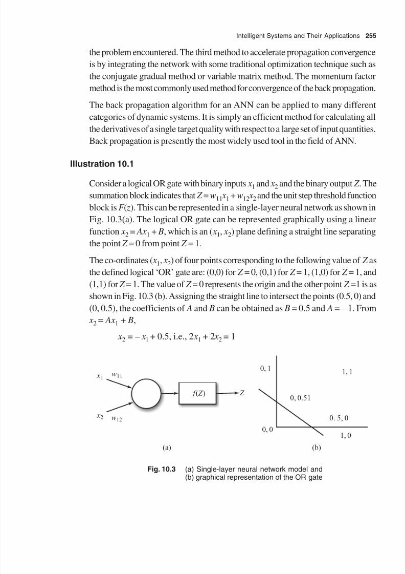
8/11/2019 Introduction to Mechatronics - Appuu Kuttan.pdf
http://slidepdf.com/reader/full/introduction-to-mechatronics-appuu-kuttanpdf 264/345
Intelligent Systems and Their Applications 255
the problem encountered. The third method to accelerate propagation convergence
is by integrating the network with some traditional optimization technique such as
the conjugate gradual method or variable matrix method. The momentum factor
method is the most commonly used method for convergence of the back propagation.
The back propagation algorithm for an ANN can be applied to many different
categories of dynamic systems. It is simply an efficient method for calculating all
the derivatives of a single target quality with respect to a large set of input quantities.
Back propagation is presently the most widely used tool in the field of ANN.
Illustration 10.1
Consider a logical OR gate with binary inputs x 1 and x 2 and the binary output Z . The
summation block indicates that Z = w11 x
1 + w
12 x
2and the unit step threshold function
block is F ( z). This can be represented in a single-layer neural network as shown in
Fig. 10.3(a). The logical OR gate can be represented graphically using a linear
function x 2 = Ax 1 + B, which is an ( x 1, x 2) plane defining a straight line separating
the point Z = 0 from point Z = 1.
The co-ordinates ( x 1, x 2) of four points corresponding to the following value of Z as
the defined logical ‘OR’ gate are: (0,0) for Z = 0, (0,1) for Z = 1, (1,0) for Z = 1, and
(1,1) for Z = 1. The value of Z = 0 represents the origin and the other point Z =1 is as
shown in Fig. 10.3 (b). Assigning the straight line to intersect the points (0.5, 0) and
(0, 0.5), the coefficients of A and B can be obtained as B = 0.5 and A = – 1. From
x 2 = Ax 1 + B,
x 2 = – x 1 + 0.5, i.e., 2 x 1 + 2 x 2 = 1
x1 w11
x2 w12
Z
(a)
1, 10, 1
0, 0.51
0. 5, 0
1, 00, 0
(b)
f Z ( )
Fig. 10.3 (a) Single-layer neural network model and(b) graphical representation of the OR gate
8/11/2019 Introduction to Mechatronics - Appuu Kuttan.pdf
http://slidepdf.com/reader/full/introduction-to-mechatronics-appuu-kuttanpdf 265/345
256 Introduction to Mechatronics
This result permits one to interpret the geometrical single-layer neural network output
as
Z = w11 x 1 + w12 x 2
with weights w11 = 2 and w12 = 2. The straight line Z = 0 separates the plane ( x 1, x 2)
as follows:
∑ For Z greater than 1, the plane above the line is defined.
∑ For Z less than 1, the plane below the line is defined.
The threshold function f ( z) corresponding to a step function can be defined as Z = 0
for f ( z) = 1 and Z = 1 for f ( z) > 1. This equation permits one to define the single-
layer neural network with weights w11 = 2 and w12 = 2. The threshold function is
f ( z) =
for Z = 2 x 1 + 2 x 2 £ 1
for Z = 2 x 1 + 2 x 2 > 1
and the output is
Z = f ( z)
The resulting neural network can be verified for the set of four values of the logical
OR gate as shown in Table 10.1. The truth table for the single-layer neural network
model is shown in Table 10.2.
Table 10.1 Truth table of the OR gate
x 1 0 0 1 1
x 2 0 1 0 1
Z 0 1 1 1
Table 10.2 Truth table of the single-layer neural network model
x 1 0 0 1 1
x 2 0 1 0 1
Z 0 2 2 4
F ( Z ) 0 1 1 1
This neural network for the OR gate has been obtained based on geometric
consideration. A training algorithm is used to obtain weight functions w11 and w12 in
a complex system. A single-layer neural network serves as a model for a system
with much reduced complexity.

8/11/2019 Introduction to Mechatronics - Appuu Kuttan.pdf
http://slidepdf.com/reader/full/introduction-to-mechatronics-appuu-kuttanpdf 266/345
Intelligent Systems and Their Applications 257
10.2 Genetic Algorithm
Genetic algorithms are search algorithms based on the mechanics of natural selection
and natural genetics. These algorithms were first developed by John Holland in
collaboration with his colleagues, and students at the University of Michigan. The
goals of their research were two fold:
1. To abstract and rigorously explain the adaptive processes of natural systems.
2. To design artificial system software that retains the important mechanisms of
natural systems.
This approach has led to important discoveries in both natural and artificial systems’
science. The control theme of research on genetic algorithms has been robustness,
the balance between efficiency and survival in many different environments.
Three main types of search methods are used conventionally. They are calculus-
based, enumerative, and random methods. We will discuss the calculus-based methodsin some detail here. These methods are subdivided into two main classes, direct and
indirect. The direct method is a well-defined computation procedure that takes some
value, or set of values as input and produces some value, or set of values, as output.
In the direct method, a sequence of computational steps transforms the input into
the output. For example, there may be a sequence of numbers which is to be sorted
in a decreasing order. This problem arises frequently in practice. This is called the
sorting problem. For the sequence (31, 41, 59, 26, 41, 58), a sorting algorithm will
return the sequence (26, 31, 41, 41, 58, 59) as the output. The indirect method seeks
local extremes by solving a non-linear set of equations resulting from setting thegradient of the objective function equal to zero. Depending upon the restrictive
requirements, continuity, and derivative existence, calculus-based methods are
unstructured for all types of the problems. These methods are insufficiently robust
in unintended domains. Enumerative scales have been considered in many shapes
and sizes. The enumerative method is a very human kind of search; such a scheme
must ultimately discount in the robustness race for one single reason of lack of
efficiency. Random search methods have achieved increasing popularity. The genetic
algorithm is an example of the search procedure that uses random chance as the
tool to guide a highly explanative search through a coding of parameters, for example,speed. Genetic algorithms differ from other types of algorithm in some very
fundamental ways:
1. Genetic algorithms work with coding of the parameter set, not the parameter
itself.
2. Such algorithms search from a population of points, not from a single point.
3. Genetic algorithms use pay-off information, not derivatives or other
accumulating knowledge.
8/11/2019 Introduction to Mechatronics - Appuu Kuttan.pdf
http://slidepdf.com/reader/full/introduction-to-mechatronics-appuu-kuttanpdf 267/345
258 Introduction to Mechatronics
4. Genetic algorithms are themselves probabilistic; these do not use deterministic
rules.
5. Genetic algorithms require a natural parameter set of the optimization problem
to be coded as a finite length string over some finite alphabets.
The mechanics of a simple genetic algorithm is simple and involves nothing morecomplex than copying a string and swapping particle strings. The system of operation
and power of effect are main attractions of the genetic algorithm approach. A
simple genetic algorithm that yields good results in many practical problems is
composed of three operations:
∑ reproduction
∑ crossover
∑ mutation
Reproduction is the process in which individual strings are copied according to theirobjective function values; biologically, this function is a fitness function. Copying of
strings according to their fitness values means that strings with a higher value have
higher probability of contributing one or more offspring in the next generation. In
natural population, fitness is determined by a creative ability to survive predators,
pestilence and other obstacles and subsequent reproduction. The reproduction operator
may be implemented in the algorithm in a number of ways. The easiest way is to
create a bias roulette wheel, where each current string in the population has a
roulette wheel sized in proportion to its fitness. After reproduction, a single crossover
may proceed in two steps. First, a number of newly reproduced strings mate at
random. Secondly, each pair of strings undergoes a crossover. The mechanics of
reproduction and crossover consists of random number of generation, string copies,
and some potential string exchange. The combined emphasis of reproduction and
the structured, through randomized, information exchange of crossover gives the
genetic algorithm much of its power. Mutation is needed, because even though
reproduction and crossover effectively search and recombine extent notaries
occasionally, the strings become overzealous and loose some potentiality and useful
genetic material. In artificial genetic systems, the mutation operator protects against
such an unrecoverable loss.
The mutation operator plays a secondary role in the simple genetic algorithm. Thefrequency of mutation to obtain good results in empirical genetic algorithm studies is
of the order of one mutation per thousand bit position transfers. Mutation rates are
similarly small in natural populations, leading to the conclusion that mutation is an
appropriate secondary mechanism of genetic algorithm adoption. Other genetic
operator of reproductive plans has been abstracted from the biological examples.
Reproduction, simple crossover, and mutation have proved to be both computationally
simple and effective in attacking a number of optimization problems and new design
techniques.

8/11/2019 Introduction to Mechatronics - Appuu Kuttan.pdf
http://slidepdf.com/reader/full/introduction-to-mechatronics-appuu-kuttanpdf 268/345
Intelligent Systems and Their Applications 259
Illustration 10.2
Consider the black box switching problem with a bank of five input switches. For
every setting of the five switches, there is an output signal g . Mathematically, f =
f (s), where s is a particular setting of the five switches. The objective of the problem
is to set the switches to obtain the maximum possible value using a genetic algorithm.
Let us first code the switches as a finite length string. A string over a finite set S is
a sequence of elements of S. For example, there are 8 binary strings for length 3,
i.e., 000, 001, 010, 011, 100, 101, 110, and 111. A switch is represented by 1 if it is on
and by 0 if it is off. Other technique for solving this problem might start with one set
of switch setting. Apply the same from citation rules and generate a new trial switch
setting. Our genetic algorithm starts with a population of strings and, thereafter,
generating successive populations of strings. For generating genetic algorithm studies,
consider four strings at random, A1= 01101, A2 = 11000, A3 = 01000, and A4 = 10011.After this, successive populations are generated using the genetic algorithm. The
population used is chosen at random through 20 successive flips of an unbiased coin.
The reproduction operator may be implemented in the algorithm form in a number of
ways. The easiest way is to create a biased roulette wheel, where each current
string has a roulette wheel slot size in proportion to its fitness. Fitness value of
objective function value may be a measure of profit, utility, or goodness which one
wants to maximize. Strings with higher values of fitness have a higher probability of
contribution to one or more offspring. After a number of spins, let the fitness be 169,
516, 640, and 361 for A1, A2, A3, and A4, respectively. Summing the fitness over allfour strings, we obtain the total fitness as 1170. Then, percentages of population of
the total fitness are 14.4%, 49.2%, 5.5% and 30.9% for A1, A2, A3, and A4,
respectively. The weighted roulette wheel for the generation reproduction is shown
A4
A3
A1
A2
49.2
5.5
30.9 14.4
Fig. 10.4 Allocation of offspring string using roulette wheel

8/11/2019 Introduction to Mechatronics - Appuu Kuttan.pdf
http://slidepdf.com/reader/full/introduction-to-mechatronics-appuu-kuttanpdf 269/345

8/11/2019 Introduction to Mechatronics - Appuu Kuttan.pdf
http://slidepdf.com/reader/full/introduction-to-mechatronics-appuu-kuttanpdf 270/345
Intelligent Systems and Their Applications 261
Fig. 10.5 (a) Aristotelian logic and (b) fuzzy logic
Illustration 10.3
During the manual operation of CNC machining, when the operator sends extra
cutting force on the tool, he overrides the feed rate with the help of ‘<’ or ‘>’ button
on the control panel. This performs an increase or decrease in the percentage of
feed rate from the programmed feed rate in the process part program. The role of
the operator can be easily substituted using an adaptive control package with a
fuzzy logic tool box. The variation in the membership function for different speeds
and depths of cut is obtained for a particular process parameter operational signal.
The fuzzy logic tool box is used to create and edit the fuzzy inference system using
a graphical tool or command line function. A fuzzy inference system is the actual
process of mapping from a given input to output. The various steps involved in the
inference system are as follows:
1. Fuzzifying input–– All the fuzzy states are resolved in the antecedent to a degree
of membership between 0 and 1.
2. Applying the fuzzy operator if there are multiple parts to be antecedent–– The
fuzzy logic operator is supplied and the antecedent of a single member between
0 and 1 is resolved.
3. Applying the implication method to resolve the degree of support for the entire
rule is used to shape the output of fuzzy set–– The consequent of the fuzzy rule
assigns an entire fuzzy set to the output. If the antecedent is only partially true,
then the output fuzzy set is processed according to the implication method.

8/11/2019 Introduction to Mechatronics - Appuu Kuttan.pdf
http://slidepdf.com/reader/full/introduction-to-mechatronics-appuu-kuttanpdf 271/345
262 Introduction to Mechatronics
4. Aggregation of all output where each rule is unified by joining parallel threads–
–The output of the aggregation process is one fuzzy set for each output variable.
5. Defuzzification–– The fuzzy set of the previous step is input to generate a
single number of crispness. The operation signal may be a process output
parameter, say, cutting force. The fuzzy output can be used for fine control
during machining. Process of fuzzification of the input and its final
defuzzification is illustrated in Fig. 10.6. Fuzzification is the process of
converting input and output values into the membership function. In this
example, among the two inputs, spindle speed is fuzzified as low, medium, or
high and depth of cut, as low, medium, or large. The output is fuzzfied as low,
moderate, and high.
Fuzzy input
(a) If the spindle speed is low or depth of cut is smaller, then the cutting force is low (Rule 1).
(b) If the speed is average of depth of cut medium, then the cutting force is moderate (Rule 2).
(c) If the speed is high or depth of cut is large, then the cuttingforce is high (Rule 3).
Output: 16.6%
Fig. 10.6 Fuzzy inference system
Fuzzy inference rule base is the controller part of the system. The rule base is
a collection of rules related to the fuzzy sets, the input variables, and the output
variables and is meant to allow the system to decide what to do in each case.
In this case, three fuzzy inference rules are used as indicated in Fig. 10.6.

8/11/2019 Introduction to Mechatronics - Appuu Kuttan.pdf
http://slidepdf.com/reader/full/introduction-to-mechatronics-appuu-kuttanpdf 272/345
Intelligent Systems and Their Applications 263
Defuzzification is the conversion of the fuzzy output value into an equivalent
crisp value for actual use. As fuzzy rules are evaluated and corresponding
values are calculated for different output fuzzy sets, there are a number of
different possibilities for defuzzification. Two common and useful techniques
are the centre of gravity method and Mamdani’s inference method. In thecentre of gravity method, the membership value for each output variable is
multiplied by the maximum singleton value of the output membership from
the membership set in question. For example, suppose that the values obtained
for the machining system membership sets are 0.4 for low and 0.6 for medium
and further suppose that the singleton value for low is 10% and for medium
is 21%, then the output value for the machining is 0.4 ¥ 10% + 0.6 ¥ 21% /
(0.4 + 0.6) = 16.6%.
In Mamdani’s inference method, the membership function of each set is
truncated at the corresponding membership value as shown in Fig. 10.6. The
resulting membership function is then added together as an OR function. This
means that all the areas that are repeated are superimposed over each other
as one layer only. The result will be a new area that is a representation of all
areas. The centre of gravity of the resulting area will be the equivalent output.
Most programs calculate the area by integrating the area under the curve.
Hand calculation may be done. In this case, the value is 16.6%, which can be
used to control the feed rate of the machine tool. A millinewton variation in
cutting force is used to control the feed rate.
10.4 Nonverbal Teaching
The growth of information technology and electronics technology has made a great
change in almost all walks of life. It has helped generate and disseminate knowledge
across the globe. Today knowledge is the most valuable and most traded resource.
Knowledge is different from all other kinds of resources. It constantly makes itself
obsolete. Knowledge can be of two kinds, explicit and tacit. Explicit knowledge is
easy to communicate through data, formulae, manuals, etc. Tacit knowledge is highlypersonal, hard to formulate, and difficult to communicate or store with a key. Welding
and painting are examples of tacit knowledge. The knowledge of a certain creation
is an interaction between explicit and tacit knowledge. The transformation of tacit
knowledge into explicit knowledge creates new knowledge. New knowledge is created
by an individual. Knowledge can create significant advantages. Conversion of tacit
knowledge into explicit knowledge at a fast rate can be achieved by nonverbal
teaching.
8/11/2019 Introduction to Mechatronics - Appuu Kuttan.pdf
http://slidepdf.com/reader/full/introduction-to-mechatronics-appuu-kuttanpdf 273/345
264 Introduction to Mechatronics
Painting is a skilled job that can be made by an experienced painter. If the painting
gun is held very close to the body to be painted, paint drops will fall on the surface
due to excess paint being projected on the surface. If the painting gun is held far
away from the body, much paint will be carried away by the air without sticking to
the body. An experienced painter will observe the body to be painted and willmanipulate the distance between the body and the painting gun to get the correct
position. If position sensors are used in the painting gun, when the painter performs
the painting operation, the coordinate positions can be stored in a computer. For a
trainee, the stored computer data acts as an instruction for the particular movement
of hand. Any wrong movement, and the painting gun gives a warning or mild jerk to
the hand. The trainee can adjust the painting gun as the master painter hand movement
without any prior experience of painting. The tacit knowledge of the skilled painter
can be easily transformed to help a trainee painter. This type of nonverbal teaching
is used in advanced machining systems. Computer stored data can also be used fora robot to perform better work following a trial and error method of teaching to the
robot.
10.5 Design of Mechatronic Systems
Engineering design is a complex process and involves interaction between many
sketches and disciplines. The design process for any item involves a number of
stages. The process begins with a need from a customer or client. This may be
identified through market research, which is used to establish the needs of potentialcustomer(s). The first stage in developing a design is to find out the true nature of
the need/problem. This is an important stage in that defining the need/problem
accurately makes the design serve the objectives very well. Following the analysis,
a specification of the requirement can be preferred. This will state the problem, any
constraints placed in the solution, and the criteria that may be used to judge the
quality of the design. These might be a statement of mass, dimension, type, range of
motion required, accuracy of input and output requirements of elements, interface
power requirements, operating environment, relevant standards, and codes of
practice. The next step is the generation of possible solutions. This is often termed
as the conceptual stage. Outline solutions are preferred, which are worked out in
sufficient detail to indicate the means of obtaining each of the required functions
such as the approximate size, shape, material, and cost. The various solutions are
explained and the most suitable ones are selected. The details of the selected design
are then worked out. This might require the production of the prototypes in order to
determine optimum details of the design. The selected design is then translated into
a working drawing (circuit diagram) so that the item can be made. It should not be

8/11/2019 Introduction to Mechatronics - Appuu Kuttan.pdf
http://slidepdf.com/reader/full/introduction-to-mechatronics-appuu-kuttanpdf 274/345
Intelligent Systems and Their Applications 265
considered that each stage of the design process just flows on stage by stage. There
will often be a need to return to an earlier stage and give it further consideration.
Thus, when at the stage of generating a possible solution, there might be the need to
go back and reconsider the analysis of the problem. The basis of the mechatronics
approach is considered to lie in the inclusion of the disciplines of electronics, computertechnology, and control engineering. The improved flexibility is the common
characteristic of mechatronic systems. Microprocessors and microcontrollers are
often embedded in a system so that control can be exercised. The term ‘embedded
system’ is used for a microprocessor-based system designed to control a range of
functions. The microprocessor programming is done by the manufacturer and is
burnt into the memory system and control cannot be changed by the user.
10.5.1 Mechatronic System Design
Our standard of living and the wealth of our country are dependent upon strides in
technology. The manufacturing of sophisticated products that we use in our day-to-
day life requires well designed systems and products. Most of these products are
mass produced, where least human intervention is required. To identify needs, today’s
world requires skills. A mechatronics engineer is expected to develop skills to identify
the needs during the study of design and technology.
Today, there are numerous different materials and an enormous range of information
and skills available. The process or system design should ensure efficiency, good
looks, and safety. It is important to note that the manufactured product’s use and
disposal will have some effect upon people, wildlife, and environment. The design
should make sure that the product appeals to a large number of people. A customer
always tries to buy a product that is comfortable, stylish, and gives good value for
the money spent. These features of a product form an important basis for the
designers of the product.
10.5.2 Stages in the Designing Process
Designers and technologists help us solve practical problems that arise in our daily
life situations. As an example, consider the situation in which old aged people need
to climb up and down stairs. Before attempting to figure out a solution to this problem,
it is important to analyse the situation to see the exact nature of the problem. Once
the problem is fully analysed and understood, the next step is to write a design brief.
A design brief is a short statement giving general outline of the problem to be solved.
On the other hand, there are some problems that can be solved by using one’s own
knowledge and imagination. However, to obtain the best possible solution, one should

8/11/2019 Introduction to Mechatronics - Appuu Kuttan.pdf
http://slidepdf.com/reader/full/introduction-to-mechatronics-appuu-kuttanpdf 275/345
266 Introduction to Mechatronics
keep oneself abreast of the advancements in the concerned knowledge domain.
This requires research. To research the problem, one should have a good understanding
of what is required and a clear understanding of the design limitations that will affect
the ultimate product. Based on this combined knowledge, a specification can now
be prepared. There must be an outline of specific details of the design that satisfyand identify the design limitations. The specifications of presently considered problem
are as follows:
1. The final device must either carry or assist the person in climbing up and down
the staircase.
2. It must be very easy to use and have a simple control.
3. It must be completely safe.
4. It must not obstruct the normal use of the staircase.
5. It must be neat and aesthetic.
6. It must be easy to operate.
7. The cost of the equipment should not exceed, say, Rs 30000.
All possible solutions to the design brief should now be visualized. The visualized
ideas can be drawn on a paper. These ideas may not necessarily be the best.
Using the ideas and information obtained through research, one should begin to
move towards a refined solution. A design must be sketched now. This needs to
be fine-tuned to incorporate all (or most) of the essential things listed in thespecifications. At this stage, the working drawing of the design is prepared. The
working drawing contains all the details of the design that are important to its
construction. Planning for the work ahead is the next step. This stage ensures that
work is completed in time.
Once the part drawings are ready, a prototype model can be prepared to verify its
workability. A prototype is a miniature form of the ultimate product. This is the most
interesting part of the work. It involves building, testing, and modifications, if any, of
the design to satisfy the specifications. Testing and evaluation of the design involves
checking the functionality, safety, and reliability of the designed product. At this
stage, any fine-tuning of the product can be prescribed. All such adjustments will be
documented and made part of the final design specifications. The areas of research
include basically the following.
1. Practical function
(i) Structural–– support, protection, construction
(ii) Mechanical–– minimum parts and construction

8/11/2019 Introduction to Mechatronics - Appuu Kuttan.pdf
http://slidepdf.com/reader/full/introduction-to-mechatronics-appuu-kuttanpdf 276/345
Intelligent Systems and Their Applications 267
(iii) Electrical–– operation and construction
(iv) Energy transfer–– mode of energy transfer
2. Shape and form
(i) Aesthetic quality, ergonomics
(ii) Shape, stability, rigidity, safety
(iii) Aerodynamics, surface texture, finish, and colour
3. Material properties
(i) Strength, hardness, toughness, ductility
(ii) Thermal conductivity, durability
(iii) Material cost
4. Construction
(i) Cutting–– shaping, filing, drilling, etc.
(ii) Fabrication–– assembly of parts using screws, bolts, glass, solder, etc.
(iii) Moulding–– application of moulds
(iv) Casting–– use of mould to cast shapes, solidification of materials
5. Sales and environment effect
(i) Manufacture, use, and dispose
(ii) Health, safety factor, noise, and smell
(iii) Aesthetic quality and pollution
Finally, a report must be prepared about the project, in which the designing process
can be illustrated using a flow chart, as shown in Fig. 10.7. A flow chart is a simple,
step-by-step, logical flow of actions oriented at a common, complex objective/product.
The thick arrows in the flow chart show the general progression of activities from
one step to the next. However, one must keep in mind that this progression is not so
simple and more often needs some lateral inputs in the form of feedback/
reinforcement at each stage. The long up-arrow on the side of the flow chart
represents this feedback/reinforcement parameter. Documentation helps in achieving
standardization of the product as per the specifications. It ensures a uniform product
quality even when the same is being manufactured at more than one location.
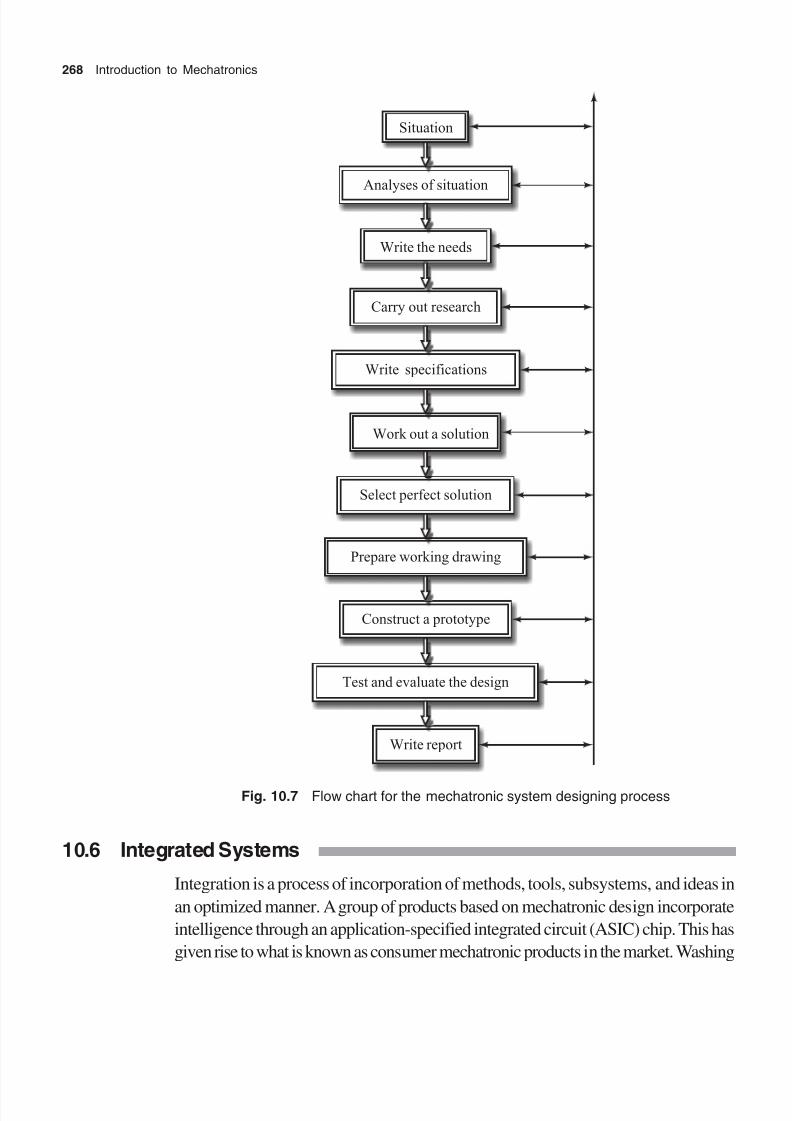
8/11/2019 Introduction to Mechatronics - Appuu Kuttan.pdf
http://slidepdf.com/reader/full/introduction-to-mechatronics-appuu-kuttanpdf 277/345

8/11/2019 Introduction to Mechatronics - Appuu Kuttan.pdf
http://slidepdf.com/reader/full/introduction-to-mechatronics-appuu-kuttanpdf 278/345
Intelligent Systems and Their Applications 269
machines, automatic cameras, bathroom scales, inkjet printers, laser printers, alarm
indicators, data loggers, toys, etc. are examples of consumer mechatronic products
which are based on the integration concept. In the following subsections, we will
discuss the design principles of some of these consumer mechatronic products.
10.6.1 Washing Machine System
Figure 10.8 shows the basic washing machine system. It gives a basic idea of the
constituent elements of a washing machine. It is a mechanical system involving a
set of cam-operated switches. When the machine is switched on, the electric motor
slowly rotates its shafts, giving an amount of rotation proportional to time. Its rotation,
in turn, controls the cams so that each cam operates electricals switches and switch
circuits in the correct sequence. The contour of a cam determines the time at which
it operates the switch. Thus, contours of the cams are the means by which thewashing program is specified and stored in the machine. The instructions used in a
particular washing program, and their sequence, are determined by a set of cam
chosen. The modern washing machine controller is a microprocessor where the
program is not guided by the mechanical arrangement of the cam.
Clock
Program
Pump
Valve
Heater
Water
Controlunit
Washingmachine
Output
Fig. 10.8 Washing machine system
For a prewash cycle, an electrically operated valve is opened when current is supplied.
This valve allows cold water into the drum for a period of time, which is determined
by the profile of the cam. The output from the microprocessor is used to operate the
switch. However, since a specific level of water in the washing machine drum is
required, there need to be another mechanism that will stop the water going into the
drum during the permitted time when it reaches the required level. A sensor is used
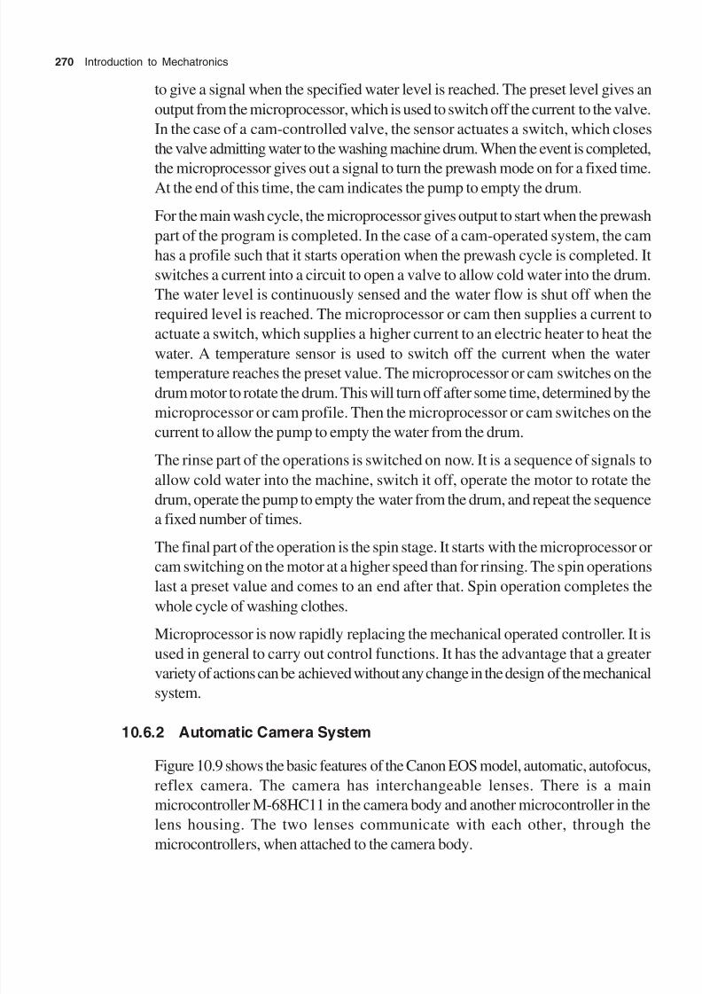
8/11/2019 Introduction to Mechatronics - Appuu Kuttan.pdf
http://slidepdf.com/reader/full/introduction-to-mechatronics-appuu-kuttanpdf 279/345
270 Introduction to Mechatronics
to give a signal when the specified water level is reached. The preset level gives an
output from the microprocessor, which is used to switch off the current to the valve.
In the case of a cam-controlled valve, the sensor actuates a switch, which closes
the valve admitting water to the washing machine drum. When the event is completed,
the microprocessor gives out a signal to turn the prewash mode on for a fixed time.At the end of this time, the cam indicates the pump to empty the drum.
For the main wash cycle, the microprocessor gives output to start when the prewash
part of the program is completed. In the case of a cam-operated system, the cam
has a profile such that it starts operation when the prewash cycle is completed. It
switches a current into a circuit to open a valve to allow cold water into the drum.
The water level is continuously sensed and the water flow is shut off when the
required level is reached. The microprocessor or cam then supplies a current to
actuate a switch, which supplies a higher current to an electric heater to heat the
water. A temperature sensor is used to switch off the current when the water
temperature reaches the preset value. The microprocessor or cam switches on the
drum motor to rotate the drum. This will turn off after some time, determined by the
microprocessor or cam profile. Then the microprocessor or cam switches on the
current to allow the pump to empty the water from the drum.
The rinse part of the operations is switched on now. It is a sequence of signals to
allow cold water into the machine, switch it off, operate the motor to rotate the
drum, operate the pump to empty the water from the drum, and repeat the sequence
a fixed number of times.
The final part of the operation is the spin stage. It starts with the microprocessor or
cam switching on the motor at a higher speed than for rinsing. The spin operations
last a preset value and comes to an end after that. Spin operation completes the
whole cycle of washing clothes.
Microprocessor is now rapidly replacing the mechanical operated controller. It is
used in general to carry out control functions. It has the advantage that a greater
variety of actions can be achieved without any change in the design of the mechanical
system.
10.6.2 Automatic Camera System
Figure 10.9 shows the basic features of the Canon EOS model, automatic, autofocus,
reflex camera. The camera has interchangeable lenses. There is a main
microcontroller M-68HC11 in the camera body and another microcontroller in the
lens housing. The two lenses communicate with each other, through the
microcontrollers, when attached to the camera body.
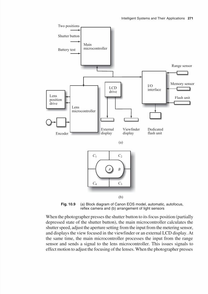
8/11/2019 Introduction to Mechatronics - Appuu Kuttan.pdf
http://slidepdf.com/reader/full/introduction-to-mechatronics-appuu-kuttanpdf 280/345
Intelligent Systems and Their Applications 271
Mainmicrocontroller
Two positions
Shutter button
Battery test
Lens position
driveLensmicrocontroller
Encoder
LCDdrive
Externaldisplay
Viewfinder display
Dedicatedflash unit
I/Ointerface
Range sensor
Memory sensor
Flash unit
A B
C 3
C 2
C 4
C 1
(a)
(b)
Fig. 10.9 (a) Block diagram of Canon EOS model, automatic, autofocus,reflex camera and (b) arrangement of light sensors
When the photographer presses the shutter button to its focus position (partially
depressed state of the shutter button), the main microcontroller calculates the
shutter speed, adjust the aperture setting from the input from the metering sensor,
and displays the view focused in the viewfinder or an external LCD display. At
the same time, the main microcontroller processes the input from the range
sensor and sends a signal to the lens microcontroller. This issues signals to
effect motion to adjust the focusing of the lenses. When the photographer presses

8/11/2019 Introduction to Mechatronics - Appuu Kuttan.pdf
http://slidepdf.com/reader/full/introduction-to-mechatronics-appuu-kuttanpdf 281/345
272 Introduction to Mechatronics
the shutter button to its click position (fully depressed state of the shutter button), the
main microcontroller issues signals to drive the microprocessor to change the aperture
to that required, open the shutter to the required exposure time, and then the shutter
closes to change to the film ready position for the next photograph.
The main microcontroller has six light sensors arranged on it, as shown in Fig. 10.9(b).Signal conditioning is used to obtain the average values of C 1, C 2, C 3, and C 4. The
A, B, and range value of C are then analysed to find the required exposure value.
This, for example, reveals whether the object is seen with a relatively constant
luminosity or perhaps a close-up of a person so that there is a bright central zone
surrounded by a dark background. The type of program used is as follows:
1. If B is equal to A and C minus B is less than 0, then exposure is set on the value
of B.
2. If B is equal to A and C minus B is 0, then exposure is set on the value of
C .This information is translated by the microcontroller into an appropriate shutter speed
and aperture value.
The range sensor has two 48-bit linear array of photodetectors. The light from the
object, after passing through the camera lens, falls on this array. When the range is
focusing the spacing of the fringes on the detector array for a particular value, if the
spacing deviates from the original then the image is out of focus. The value of this
deviation is used to give an error signal, which is fed to the lens microcontroller and
used to give a warning to adjust the focusing of the lens. An encoder is used to
provide feedback for this adjustment so that the microcontroller knows when thefocusing has been completed.
The iris diaphragm drive system is a stepper motor which opens or closes a set of
diaphragm blades. The focusing operation involves two forms of drives: arc-form
drive and ultrasonic motor. The arc-form drive is used to run a brushless permanent
magnet DC motor. A Hall sensor is used to detect the position of a rotor. The drive
from the motor is transmitted through gears to move the focusing lens along the
optical axis. The ultrasonic motor has a series of piezoelectric elements in the form
of a ring. By switching on current through the piezoelectric elements in an appropriate
sequence, a displacement wave can be made to travel along the ring of elements ineither a clockwise or counterclockwise direction. This, consequently , rotates a
rotor, which is in contact with the surface of the ring elements, hence driving the
focusing element.
10.6.3 Inkjet Printer System
The inkjet printer uses a conductive ink, which is forced through a small nozzle to
produce a jet of very small drops of ink of constant diameter at constant frequency.

8/11/2019 Introduction to Mechatronics - Appuu Kuttan.pdf
http://slidepdf.com/reader/full/introduction-to-mechatronics-appuu-kuttanpdf 282/345

8/11/2019 Introduction to Mechatronics - Appuu Kuttan.pdf
http://slidepdf.com/reader/full/introduction-to-mechatronics-appuu-kuttanpdf 283/345
274 Introduction to Mechatronics
the beam of light, parts on the drum can be discharged or left charged. As the drum
passes over the toner reservoir, the charged area attracts particles of the toner. The
toner particles stick to the areas that have not been exposed to light, leaving out the
areas that have been exposed to light. The sheet of paper is given a charge as it
passes along another charging wire, the so-called corona wire. When this chargedpaper passes along the drum, it attracts the toner off the drum. A hot passing roller
is then used to melt the toner particles so that, after passing between rollers, the
finishings adhere to the sheet of paper. Laser printers currently in use are able to
produce 600 dots per 25 mm. Figure 10.11 illustrates the working principle of the
laser printer.
Laser beam
Coron wire
Fusing roller
Selenium drum
Charging wire
Fig. 10.11 Basic elements of a laser printer
10.6.5 Bathroom Scale System
Consider the design of a simple weighing machine, called bathroom scale. The
objective of this device is that a person can stand on a platform and the weight of
that person should be displayed as some form of read-out. The weight should be
given with reasonable speed and accuracy and irrespective of the location of the
person on the platform. One possible solution may be to use the weight of the person
on the platform to deflect an arrangement of two parallel leaf springs. With such an
arrangement, the deflection is virtually independent of where on the platform the
person stands. The deflection can be transformed into a movement of a plate across
the scale by using the arrangement shown in Fig. 10.12. A rack and pinion
arrangement is used to transform the linear motion into a circular motion about the
horizontal axis. This is then transformed into a rotation about the vertical axis, and
hence into the movement of a pointer across a scale.

8/11/2019 Introduction to Mechatronics - Appuu Kuttan.pdf
http://slidepdf.com/reader/full/introduction-to-mechatronics-appuu-kuttanpdf 284/345
Intelligent Systems and Their Applications 275
Load
Leaf spring
(a) Platform detector (b) Rack and pinion arrangment
Active strain Differentialamplifier
PC0PC1
P80P81P82P83P84
M68H11
(c) Microcontroller system
Fig. 10.12 Bathroom scales
Another possible solution involves the use of a microprocessor. The platform can be
mounted on load cells employing electrical resistance strain gauges. When the person
stands on the platform, the gauges suffer strain and change resistance. If the gaugesare mounted in a four-active-arm Wheatstone bridge, then when out of balance, the
voltage output from the bridge is a measure of the weight of the person. The outpu
voltage can be amplified by a differential operational amplifier. The resulting analog
signal can then be fed through a latched analog to digital converter for inputting to
the microprocessor. If a microcontroller is used, then, memory is present within a
microprocessor chip, and by a suitable choice of microcontroller, the output can be
calculated. For instance, M68HC11 can obtain analog to digital conversion for inputs
The output can be passing through a suitable decoder to give an LED display.
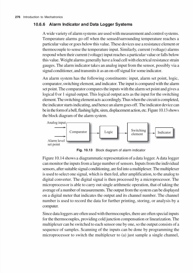
8/11/2019 Introduction to Mechatronics - Appuu Kuttan.pdf
http://slidepdf.com/reader/full/introduction-to-mechatronics-appuu-kuttanpdf 285/345
276 Introduction to Mechatronics
10.6.6 Alarm Indicator and Data Logger Systems
A wide variety of alarm systems are used with measurement and control systems.
Temperature alarms go off when the sensed/surrounding temperature reaches a
particular value or goes below this value. These devices use a resistance element or
thermocouple to sense the temperature input. Similarly, current (voltage) alarms
respond when their current (voltage) input reaches a particular value or falls below
this value. Weight alarms generally have a load cell with electrical resistance strain
gauges. The alarm indicator takes an analog input from the sensor, possibly via a
signal conditioner, and transmits it as an on-off signal for some indicator.
An alarm system has the following constituents: input, alarm set point, logic,
comparator, switching element, and indicator. The input is compared with the alarm
set point. The comparator compares the inputs with the alarm set point and gives a
logical 0 or 1 signal output. This logical output acts as the input for the switchingelement. The switching element acts accordingly. Thus when the circuit is completed,
the indicator starts indicating, and hence an alarm goes off. The indicator device can
be in the form of a bell, flashing light, siren, displacement action, etc. Figure 10.13 shows
the block diagram of the alarm system.
Comparator Logic Switchingelement Indicator
Analog input
Alarm level
set point
Fig. 10.13 Block diagram of alarm indicator
Figure 10.14 shows a diagrammatic representation of a data logger. A data logger
can monitor the inputs from a large number of sensors. Inputs from the individual
sensors, after suitable signal conditioning, are fed into a multiplexer. The multiplexer
is used to select one signal, which is then fed, after amplification, to the analog to
digital converter. The digital signal is then processed by a microprocessor. The
microprocessor is able to carry out single arithmetic operation, that of taking the
average of a number of measurements. The output from the system can be displayedon a digital meter that indicates the output and its channel number. The channel
number is used to record the data for further printing, storing, or analysis by a
computer.
Since data loggers are often used with thermocouples, there are often special inputs
for the thermocouples, providing cold junction compensation or linearization. The
multiplexer can be switched to each sensor one by one, so the output consists of a
sequence of samples. Scanning of the inputs can be done by programming the
microprocessor to switch the multiplexer to (a) just sample a single channel,

8/11/2019 Introduction to Mechatronics - Appuu Kuttan.pdf
http://slidepdf.com/reader/full/introduction-to-mechatronics-appuu-kuttanpdf 286/345
Intelligent Systems and Their Applications 277
(b) carry out a single scan of all channels, (c) a continuous scan of all channels, or
(d) carry out a periodic scan of all channels, say, every 1, 8, 15, 30, 60 min. Typically,
a data logger may handle 20–100 inputs, though some may handle considerably
more, about 1000. A blogger may have a sample and conversion time of 10 ns and
be used to make 1000 readings/sec. The accuracy is typically about 0.01% andlinearity is about ±0.005% of full scale input. Cross-talk is typically 0.01% of the full
scale input or any one input. The term cross-talk is used to describe the interference
that can occur as a result of signals from other sensors while a sensor is being sampled.
Digitalsignal
Analogsignal
Digitalmultiplexer
Analogmultiplexer
Cold junctioncompensator
Amplifier ADC
Microprocessor
Display, printer,floppy,others
Remotecontrol
Fig. 10.14 Data logger system
Case Study 10.1: Slip Casting Process
Slip casting is used as the primary manufacturing process for many complex ceramic
products when ceramic pressing is not practical, e.g., in the manufacturing of
sanitaryware, giftware, tableware, etc. Slip casting is generally the second choice
because it is considerably more difficult to achieve good results in both product
quality and productivity. Pressing has the drawback in that it can only manufactureproducts of simple shapes. However, slip casting can be employed to manufacture
items such as bowels, pitchers, statues, and sinks. The manufacturing of slip casting
ceramicware involves the following steps:
1. Preparation of slip (clay)
2. Casting the slip in a plastic mould for a specified duration
3. Removing the mould
4. Air-drying the cast piece
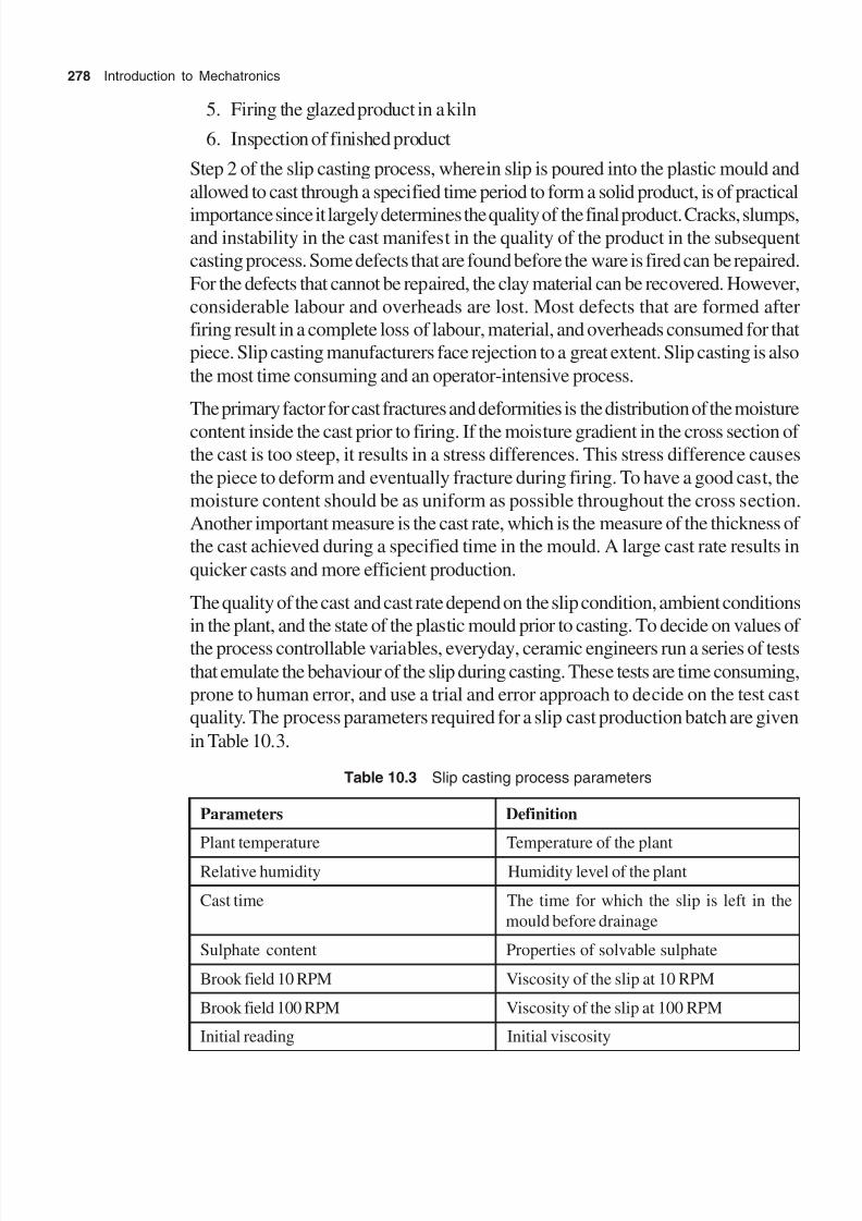
8/11/2019 Introduction to Mechatronics - Appuu Kuttan.pdf
http://slidepdf.com/reader/full/introduction-to-mechatronics-appuu-kuttanpdf 287/345
278 Introduction to Mechatronics
5. Firing the glazed product in a kiln
6. Inspection of finished product
Step 2 of the slip casting process, wherein slip is poured into the plastic mould and
allowed to cast through a specified time period to form a solid product, is of practical
importance since it largely determines the quality of the final product. Cracks, slumps,and instability in the cast manifest in the quality of the product in the subsequent
casting process. Some defects that are found before the ware is fired can be repaired.
For the defects that cannot be repaired, the clay material can be recovered. However,
considerable labour and overheads are lost. Most defects that are formed after
firing result in a complete loss of labour, material, and overheads consumed for that
piece. Slip casting manufacturers face rejection to a great extent. Slip casting is also
the most time consuming and an operator-intensive process.
The primary factor for cast fractures and deformities is the distribution of the moisture
content inside the cast prior to firing. If the moisture gradient in the cross section ofthe cast is too steep, it results in a stress differences. This stress difference causes
the piece to deform and eventually fracture during firing. To have a good cast, the
moisture content should be as uniform as possible throughout the cross section.
Another important measure is the cast rate, which is the measure of the thickness of
the cast achieved during a specified time in the mould. A large cast rate results in
quicker casts and more efficient production.
The quality of the cast and cast rate depend on the slip condition, ambient conditions
in the plant, and the state of the plastic mould prior to casting. To decide on values of
the process controllable variables, everyday, ceramic engineers run a series of tests
that emulate the behaviour of the slip during casting. These tests are time consuming,
prone to human error, and use a trial and error approach to decide on the test cast
quality. The process parameters required for a slip cast production batch are given
in Table 10.3.
Table 10.3 Slip casting process parameters
Parameters Definition
Plant temperature Temperature of the plant
Relative humidity Humidity level of the plant
Cast time The time for which the slip is left in the
mould before drainage
Sulphate content Properties of solvable sulphate
Brook field 10 RPM Viscosity of the slip at 10 RPM
Brook field 100 RPM Viscosity of the slip at 100 RPM
Initial reading Initial viscosity

8/11/2019 Introduction to Mechatronics - Appuu Kuttan.pdf
http://slidepdf.com/reader/full/introduction-to-mechatronics-appuu-kuttanpdf 288/345
Intelligent Systems and Their Applications 279
Build up Initial viscosity (taken at 3.5 min)
20 minute gelation Thixotropy (viscosity versus time)
Filtrate rate The rate at which the slip filter rates
Slip cake weight Approximation of the cast rate without
considering a mould
Cake weight water retention Moisture content of the cake
Slip temperature The temperature of the slip
A neural network and fuzzy logic technique can be used to improve the quality andthe efficiency of the slip casting process. A hybrid approach is adopted because the
moulds can be used individually or collectively depending on the decision to be made.The predictive module estimates the cast rate neural network (CRNN) and moisturegradient neural network (MGNN) to determine the cast quality and efficiency for
the given ambient conditions, process settings, and slip characteristic as specified inTable 10.3. The fuzzy logic expert system recommends the processing timecustomized to a production line given the localized ambient state and the conditions
of the plaster mould.
Many of the process variables are uncontrollable. For instance, ambient conditions,particle distribution of the raw material and slip properties cannot be changed onday-to-day basis. The interactive behaviour of the process variables is mostlyunquantified. The neural network is an empirical universal approximation technique.That is, a neural network can theoretically model any relationship through examination
of inputs and outputs. The neural network predictions can be used for the daily testcasts. The predictions are also used in change with the process improvement algorithmfor production control.
In this case, large data, both input specified in Table 10.3 and outputs, are considered,which contain thousands of observations in four to five years. The neural networkarchitecture, training parameters, and stopping criteria were selected through
experimentation and examination of preliminary networks. An ordinary backpropagation learning algorithm was used because of its documented ability as acontinuous approximator. With experience, it was observed that the neural networkfor CRNN was multi-layered, fully connected perception with 13 inputs, two hiddenlayers with 11 hidden neurons in each layer, and single output, which means the castrate gives a convergence result. The MGNN model was developed in the same
way, using the same input variables, two hidden layers and 27 hidden neurons ineach layer, single output, and moisture gradient percentage change.
The more traditional random separation of the data into testing and training sets is in
the ratio of 3 : 7, respectively. This system is for the industrial use. Fivefold group
validation has been used to validate the neural network as this allows all data to be
used for both validation and construction of the neural network model. The estimation

8/11/2019 Introduction to Mechatronics - Appuu Kuttan.pdf
http://slidepdf.com/reader/full/introduction-to-mechatronics-appuu-kuttanpdf 289/345
280 Introduction to Mechatronics
of the neural network prediction error by the data splitting method is not accurate or
reliable than with a single network. Finally, the neural network used in the system
can be constructed using all the data rather than just the training subset to ensure the
best possible prediction. The summation of the test set over five validation networks
showed a mean absolute error of 4.8% and 68.4% for CRNN and MGNN,
respectively. This may be due to the considerable human error in the measurement
of the moisture gradient. This imprecision, however, did not preclude the MGNN
use in the system. The MGNN does a fairly good job of prediction for a small
moisture gradient and can discriminate between a good moisture gradient and a bad
moisture gradient. Taking a categorical approach, the MGNN has a prediction ability
of adequate precision for use in the plant.
The neural network prediction model estimates the cast rate and moisture gradient
for each combination. The optimization algorithm selects the best three combinations
that minimize the moisture gradient and maximize the cast rate. Providing the threebest process settings allows the ceramic engineer to review the options prior to
implementation, imparting some human expertise in the decision making. If the user
wishes to further study the three recommended settings by considering other factors,
they can use the analytic hierarchy process.
The fuzzy logic expert system model is incorporated to consider the important factor(s)
affecting the cast quality, which is individual to a particular product line. These
factors are the age of the plastic moulds (which ranges from 0 to 6 weeks) and the
ambient conditions. It is necessary to use a knowledge-based approach rather than
a pure numeric model because there is no data that relates the mould age and localambient environment to the cast quality. It is impractical to begin to record such data
in the plant. Instead, these two important factors are included in two bases that
work as hierarchy, as shown in Fig. 10.15. The use of fuzzy logic is included to allow
more precise handling of the variables, reduce the number of rules required, and
result in a smoother decision surface.
Casting ratefrom CRNN
Mouldcondition(10 – 10)
Temperature
Humidity
Mould age
Rule base 1
Rule base 2
Productionline castingtime
Fig. 10.15 Structure of the fuzzy logic expert system module

8/11/2019 Introduction to Mechatronics - Appuu Kuttan.pdf
http://slidepdf.com/reader/full/introduction-to-mechatronics-appuu-kuttanpdf 290/345
Intelligent Systems and Their Applications 281
Referring to Fig. 10.15, the ambient temperature, relative humidity, and age of the
moulds in weeks for the production line can be presented as crisp, continuous inputs
to the first fuzzy rule base that predicts the mould conditions. The mould condition is
rated on an ordinary scale of 0 to 10, with 0 being the dirtiest and 10 being the
wettest. This prediction of the mould condition is then paired with a crisp, continuousprediction of the cast rate from CRNN. Together, these are used in the second
fuzzy rule base in order to generate a recommended cast time in minutes for a
particular production line. Defuzzification to a crisp output is done using the centroid
method, by computing the centre of mass of the region of the output variable defined
by the fuzzy output.
The hybrid modular system is a comprehensive decision support system and uses
computational intelligence for the ceramic slip casting process. The integration of
the neural network, dual optimization algorithm, and the fuzzy logic rule allowsmodelling of the highly non-linear relationship among the process variables and the
capture of qualitative factors and expert knowledge from the plant personnel.
Utilization of this system enables a casting decision to be made consistently and
correctly without the need for judgemental speculation or expensive trial and error
test casts. Figure 10.16 shows the block diagram that integrates the neural network,
dual optimization algorithm, and fuzzy logic technique to improve the quality and
efficiency of the slip casting step.
User interface Data repository
Cast rate NN Fuzzy rule bases
Moisturegradient NN
Processimprovement
Optimizational orithmg
Fig. 10.16 Block diagram of the hierarchical system of slip casting

8/11/2019 Introduction to Mechatronics - Appuu Kuttan.pdf
http://slidepdf.com/reader/full/introduction-to-mechatronics-appuu-kuttanpdf 291/345
282 Introduction to Mechatronics
Case Study 10.2: Pick-and-Place Robot
Robots are widely used in automated industries. A robot is a mechatronic system
capable to replace or assist the human operator in carrying out a variety of physical
tasks. The Webster dictionary defines robot as ‘a machine that looks like a human
being and performs various complex acts (as walking or talking) of a human being’.
An industrial robot is very difficult to define. The industrial robot continuously interacts
with the surrounding environment. This continuous interaction is achieved through
sensors and transducers. Computer-controlled interaction systems emulate human
capabilities. The Robotic Industries Association has defined the manipulation robot
used in industry as follows: ‘A robot is a reprogrammable, multifunctional manipulator
designed to move materials, parts, tools or special devices through variable
programmed motion for performing a variety of tasks.’
There is a variety of robots used in industrial applications. Broadly, they are classified
as fixed robots and mobile robots. Mobile robots are also called automated guided
vehicles (AGV) or walking robots. Fixed robots have different configurations as per
the requirement of their application in industry. Fixed robots are further classified as
cartesian robots, cylindrical robots, polar robots, and articulated arm or spline robots.
For the pick-and-place operation, usually the articulated arm robots are commonly
used. An articulated arm robot contains basically five subsystems, namely,
1. Robot arm
2. End effectors
3. Drive or actuator
4. Sensors
5. Controller
The robot arm helps position the end effector of the robot to perform the programmed
tasks. It is an open-chain mechanism like human arm. Three degrees of freedom
(transitions) can be obtained from a robot arm. In between the robot arm and endeffector, a wrist mechanism is mounted. This wrist mechanism gives three rotational
degrees of freedom to the end effector. Thus an industrial robot has six degrees of
freedom.
The end effector is a handlike tool connected to the robot arm. The work pieces
holding the end effectors are called grippers and the tools holding the end effectors
are called tool holders. A gripper may be a mechanical lever, adhesive, vacuum cup,
magnetic hook, or a snooper.

8/11/2019 Introduction to Mechatronics - Appuu Kuttan.pdf
http://slidepdf.com/reader/full/introduction-to-mechatronics-appuu-kuttanpdf 292/345
Intelligent Systems and Their Applications 283
Drives or actuators are parts of the controller element that act as per the command
of the controller and translate the signal from the controller into an operation.
Electrical, pneumatic, or hydraulic actuators can be used to perform the final actuation.
Sensors play an important role in the functioning of a robot. Both internal and external
sensors are used in a robot arm. Robots using an external sensor to identify the
external object are called smart robots.
Every robot is connected to a computer. The computer along with the necessary
software is known as the controller. The controller also allows compatibility with
other systems of the manufacturing environment. A controller with artificial
intelligence makes a robot more self-reliant and independent.
End effector
Fig. 10.17 Configuration of a jointed-arm robot
Figure 10.17 shows the configuration of a jointed-arm robot used for pick-and-place
operations. Its configuration corresponds to the human forearm. Its upper arm is
mounted on a vertical pedestrian. The components of this arm are connected by two
rotary joints corresponding to the shoulder and elbow. A wrist mechanism attached
to the end of the forearm provides three additional degrees of freedom.
A robot program is accomplished in several ways. Two basic methods to accomplish
robot programming are
∑ Lead through method
∑ Textual robot language
The lead through method requires the program to move the manipulator through the
desired motion path. It also requires that the path be committed to memory by the
robot controller. Robot programming through a textual language is accomplished
somewhat like computer programming. The programmer types in the program mode
on a cathode ray monitor (CRM) using high level English language. Textual languages

8/11/2019 Introduction to Mechatronics - Appuu Kuttan.pdf
http://slidepdf.com/reader/full/introduction-to-mechatronics-appuu-kuttanpdf 293/345
284 Introduction to Mechatronics
appeared around 1979 and are in use since then in the robot industry. To illustrate a
textual program, consider a work cell as illustrated in Fig. 10.18. A press path is
indicated by the pillar boundaries lines. The robot has to pick at point 8, 1 and drop a
tote pan at 1, 8. The point 8,1. is the position to wait for the robot to operate before
entering the press to remove the part. The robot must start from the point 1, 1, whichis a safe place for the robot during the press work. The program given in Table 10.4
accomplishes the unloading task in the press work.
8, 81, 8
1, 1 8, 1
Press columns
Fig. 10.18 Work cell
Table 10.4 Program for an unloading task in the press work
Step Signal Comments
0 1, 1 Start at home position
1 8,1 Move to wait position 1,1
2 WAIT 1,1 Wait for press to open
3 8, 8 Move to pick up point
4 SIGNAL 5 Signal gripper to close
5 8,1 Move to safe position
6 SIGNAL 4 Signal press to actuate
7 1, 1 Move around press column
8 1,8 Move to tote pan
9 SIGNAL 6 Signal gripper to open
10 1, 1 Move to safe position

8/11/2019 Introduction to Mechatronics - Appuu Kuttan.pdf
http://slidepdf.com/reader/full/introduction-to-mechatronics-appuu-kuttanpdf 294/345
Intelligent Systems and Their Applications 285
Exercises
10.1 Why are advanced mechatronic systems required in manufacturing?
10.2 Explain the working principle of an artificial neural network.
10.3 Why is the sigmoid function considered an input signal for ANN?
10.4 Explain the back propagation algorithm with examples.
10.5 How can genetic algorithms be used for process control?
10.6 What is nonverbal teaching?
10.7 What are the advantages of fuzzy logic control over conventional control
system?
10.8 Explain the application of a mechatronic system with the sequence of operation.
10.9 Explain the working of an automatic camera system.
10.10 Explain the working principles of inkjet and laser printers.
10.11 Write a short note on data logger systems.

8/11/2019 Introduction to Mechatronics - Appuu Kuttan.pdf
http://slidepdf.com/reader/full/introduction-to-mechatronics-appuu-kuttanpdf 295/345
Autotronics, Bionics, and Avionics
Mechatronic products have become increasingly dominant in every aspect of
commercial marketplace as technologies, electronics, and computers continue to be
developed. Presently major commercial markets for mechatronic products are in
the form of automobiles, aeronautical/astronautical systems, and biological systems.
The automobile industry has been the major user of mechatronics technology during
the recent decades. Another commercial application of mechatronics is in biomedical
and biological sciences. Aircraft and rocket technologies are the other areas where
the use of mechatronic systems has been growing rapidly. Advancements in
mechatronics in the areas of automobile engineering, biotechnology, and aircraft androcket engineering, have given rise to specialized disciplines of autotronics, bionics,
and avionics, respectively. We will discuss these three major specialized study areas
of mechatronics in this chapter.
11.1 Autotronics
The primary motivation for adopting mechatronic systems in automobiles is to make
automobiles safer, more comfortable, fuel efficient, and less polluting systems. A
widespread use of mechatronic products can indeed make an automobile smarterfor consumer needs. Smart vehicles are based on an extensive use of mechatronic
systems to detect the environment or road conditions. Microactuators are used to
execute whatever actions are required to deal with these conditions. The modern
car comes with many electronic control systems. As the mechatronics technology
developed, a new discipline called autotronics has emerged. The design and production
of mechatronic systems for automobiles that perform at extreme environmental
conditions presents a major challenge to engineers. Application of mechatronic
systems in automobiles is in the following major areas:

8/11/2019 Introduction to Mechatronics - Appuu Kuttan.pdf
http://slidepdf.com/reader/full/introduction-to-mechatronics-appuu-kuttanpdf 296/345
Autotronics, Bionics, and Avionics 287
∑ Safety
∑ Engine and power train
∑ Comfort and convenience
∑ Vehicle diagnostics and health monitoring
The airbag deployment system to protect the driver and passenger from injury in the
event of a serious vehicle collision is a mechatronic safety system. The antilock
braking system, air suspension system, navigation system, and obstacle avoidance
all give security to the driver and passenger.
Various mechatronic systems are used in engines of modern automobiles. Some of
these are listed below:
∑ Manifold control pressure sensor
∑ Air flow control
∑ Exhaust gas analysis and control
∑ Crankshaft position control
∑ Fuel pump pressure and fuel injection control
∑ Transmission force and pressure control
∑ Engine knocking detection for high power output
The manifold absolute pressure (MAP) system was one of the first micromechatronic
systems adapted by the automobile industry. In the early 1980s, MAP was used to
measure the engine speed in revolutions per minute (RPM) to determine the ignitionadvance. The ignition timing with optimum air/fuel ratio can optimize the power
performance of the engine with a low emission. Various mechatronic systems used
in the modern automobile engines are:
∑ Seat control for passenger comfort
∑ Defogging of wind shield
∑ Automatic dim and bright control
∑ Satellite navigation
The comfort and convenience of passengers are considered while designingmechatronic systems. For vehicle diagnostic and health monitoring, mechatronic
systems are used for monitoring the following conditions:
∑ Engine coolant temperature and quality
∑ Engine oil pressure, level, and quality
∑ Tyre pressure
∑ Transmission fluid
∑ Fuel pressure, etc.
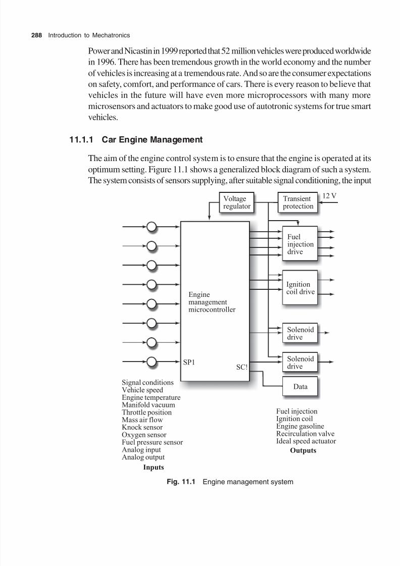
8/11/2019 Introduction to Mechatronics - Appuu Kuttan.pdf
http://slidepdf.com/reader/full/introduction-to-mechatronics-appuu-kuttanpdf 297/345
8/11/2019 Introduction to Mechatronics - Appuu Kuttan.pdf
http://slidepdf.com/reader/full/introduction-to-mechatronics-appuu-kuttanpdf 298/345
Autotronics, Bionics, and Avionics 289
signals to the microcontroller and providing output signals via the driver to actuate
actuators. The engine speed sensor is an inductance type that changes as the teeth
of the sensor wheel pass it and so gives an oscillating voltage. The temperature
sensor is usually a thermistor. The mass air flow sensor can be a hot wire anemometer
and as air passes over the heated wire, it will be cooled. The amount of coolingdepends upon the mass flow rate. The oxygen sensor is generally a closed-end tube
made of zirconium oxide with porous platinum electrodes on the inner and outer
surfaces. Above near 300oC, this sensor becomes permeable to oxygen ions and so
measures the voltage flowing between the electrodes.
The engine management system of a car is responsible for managing the ignition
and fuelling requirements of the engine. In a four-stroke internal combustion engine,
there are several cylinders, each having a piston connected to a common crankshaft
and each of which comes out of a four-stroke engine sequence of operation. Whenthe piston moves, the valve opens, and the air-fuel mixture is drawn into the cylinder.
When the piston moves down, up again, the valve closes and the air-fuel mixture is
compressed. When the piston is near the top of the cylinder, the spark plug ignites
the mixture with the resulting expansion of the hot gases. This expansion causes the
piston to move down again and so the cycle is completed. The piston of each cylinder
is connected to a common crankshaft and the power strokes occur at different
times, so that there is a continuous power supply for rotating the crankshaft. The
power and speed of the engine are controlled by varying the ignition timing and air-
fuel mixture. In the modern car engine, this is done by a microprocessor andmechatronic systems. For ignition timing, the crankshaft drives a distributor, which
makes electrical contacts with each spark plug and, in turn, with a timing wheel.
The timing wheel generates pulses to indicate the crank position. The microprocessor
then adjusts the timing at which high-voltage pulses are sent to the distributor, so
they occur at the right time. To control the amount of air-fuel mixture entering into a
cylinder during the intake strokes, the microprocessor varies the time for which a
solenoid is activated to open the intake valve on the basis of inputs received in the
form of the engine temperature and the throttle position. The amount of fuel to beinjected into the air stream can be determined by the input from a sensor on the
mass rate of air flow, or can be computed from other measurements. The
microprocessor then gives an output to control the fuel injection valve.
11.1.2 Windscreen Wiper Mechanism
For cleaning/wiping the windscreen of the car, a device that will oscillate an arm
back and forth in an arc is needed. The windscreen wiper is a mechanical device

8/11/2019 Introduction to Mechatronics - Appuu Kuttan.pdf
http://slidepdf.com/reader/full/introduction-to-mechatronics-appuu-kuttanpdf 299/345
290 Introduction to Mechatronics
that can be operated by the use of stepper motor. Figure 11.2 shows how a
programmable logic circuit (PLC) or microcontroller can be used with the stepper
motor for operating a wiper device. The stepper motor needs an input to cause it to
rotate a number of steps in one direction and then reverse the same number of steps
with the reverse direction.
14 4 13 6
8
9
11
3
2
15
SAA 1027
Fig. 11.2 Interfacing a stepper motor
If the stepper motor is to be in the full-step configuration, the output needs to be as
shown in Table 11.1. Thus to start and rotate the motor in a forward direction, it
involves the sequence A, 9, 5, 6 and then back to the start with 1 again. To reverse,
one could use the sequence 6, 5, 9, A and then back to the start with 6 again. If the
half-step configuration is used for forward motion, then it involves the sequence A,
8, 9, 1, 5, 4, 6, 2 and then back to A. To reverse, the sequence is 2, 6, 4, 5, 19, 8, A
and back to 2. If many steps involved, a single program is to increment a counter
with each step and loop control the counter value till it reaches the required number.
Table 11.1 Truth table for interfacing stepper motor
Bits Code
1 1 0 1 0 A
2 1 0 0 1 9
3 0 1 0 1 5
4 0 1 1 0 6
5 1 0 1 0 A
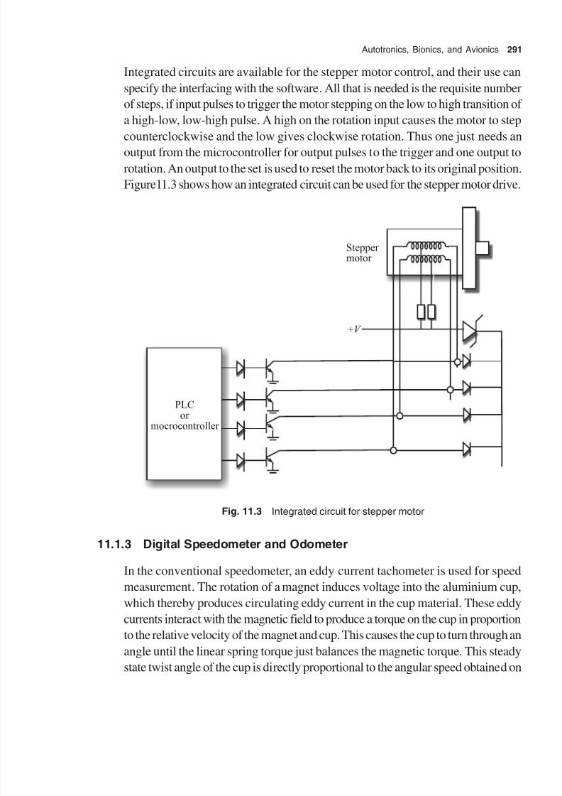
8/11/2019 Introduction to Mechatronics - Appuu Kuttan.pdf
http://slidepdf.com/reader/full/introduction-to-mechatronics-appuu-kuttanpdf 300/345
Autotronics, Bionics, and Avionics 291
Integrated circuits are available for the stepper motor control, and their use can
specify the interfacing with the software. All that is needed is the requisite number
of steps, if input pulses to trigger the motor stepping on the low to high transition of
a high-low, low-high pulse. A high on the rotation input causes the motor to step
counterclockwise and the low gives clockwise rotation. Thus one just needs anoutput from the microcontroller for output pulses to the trigger and one output to
rotation. An output to the set is used to reset the motor back to its original position.
Figure11.3 shows how an integrated circuit can be used for the stepper motor drive.
Stepper motor
+V
PLC
or mocrocontroller
Fig. 11.3 Integrated circuit for stepper motor
11.1.3 Digital Speedometer and Odometer
In the conventional speedometer, an eddy current tachometer is used for speed
measurement. The rotation of a magnet induces voltage into the aluminium cup,
which thereby produces circulating eddy current in the cup material. These eddy
currents interact with the magnetic field to produce a torque on the cup in proportion
to the relative velocity of the magnet and cup. This causes the cup to turn through an
angle until the linear spring torque just balances the magnetic torque. This steady
state twist angle of the cup is directly proportional to the angular speed obtained on

8/11/2019 Introduction to Mechatronics - Appuu Kuttan.pdf
http://slidepdf.com/reader/full/introduction-to-mechatronics-appuu-kuttanpdf 301/345
292 Introduction to Mechatronics
the wheel through the rotating cable. The conventional automobile odometer is a
drum-type mechanical counter. The counter may be driven either mechanically or
by directly coupling it to a rotating shaft or wheel, or they may be actuated by
oscillating a reciprocating motion introduced through an appropriate linkage and
ratchet mechanism. Mechanical counters that can be actuated by electrical impulsesare also available. Such electrically actuated counters may be energized by a single
switch or relay, or by photocells or by a pulse with a supply power of several watts.
One high-speed counter of this type is capable of making 1000 counts/min. Such a
counter requires a 5-W power source and responds to make a pulse as short as
0.024 sec or a break of 0.036 sec duration. In mechatronic system applications, the
angular velocity can be measured by using a combination of a toothed wheel and a
single magnetic proximity pick-up and electronic event per unit time (EPUT) meter.
The toothed iron wheel passing under the proximity pick-up produces an electrical
pulse each time a tooth passes. These pulses are fed to the EPUT meter, whichcounts them over an accurate time period and displays the result. Usually, the display
stays for a few seconds to enable reading and then repeats the process over and
over again. The inaccuracy of the pulse counting is ±1 pulse error. The high-speed
counting for the odometer electronic counter can be used. As each pulse is received,
a progressive circuit change occurs, which is indicated by the counter tube. After
ten such changes, an output pulse is produced, which can be used to drive the
following decade. A series of decades may be used in this manner to record 1’s,
10’s or 100’s, etc. The electronic counter has high impedance and requires little
energy for pulsing. Figure 11.4 illustrates the working principle of speedometer/
odometer.
N S
w
(a) Speedometer
Aluminiumcup
Pointer
ScaleOutput
(b) Induction-type speedometer
Fig. 11.4 Speedometer

8/11/2019 Introduction to Mechatronics - Appuu Kuttan.pdf
http://slidepdf.com/reader/full/introduction-to-mechatronics-appuu-kuttanpdf 302/345
Autotronics, Bionics, and Avionics 293
11.1.4 Automatic Dim and Bright Control
Photosensors can be used to control the dimness and brightness of headlights. The
circuit diagram for such an automatic dim and bright control actuation is shown in
Fig. 11.5. An operation amplifier is used to compare the voltage generated from the
photocell to the reference voltage. The operation amplifier is actuated with a volt
battery, with typical values of resistance Ra= 8.15 k W, R1 = 1 k W, and Rg = 100 k W.
When a vehicle from the opposite direction is within the range of the source vehicle,
the light from the opposite vehicle actuates a detector and the analog input actuates
a relay to adjust to the dim light.
Fig. 11.5 Automatic dim and bright control system
11.1.5 Radiator Water Level Indicator and Control of Radiator Fan
The level of liquid in a vessel can be measured by monitoring the position of theliquid surface indirectly by measuring some variables related to the height. Direct
methods involve floats and the indirect method includes the monitoring of weight of
the vessel. The weight of the liquid is proportional to its height. A direct method of
monitoring the level of liquid in a radiator is made easier by monitoring the movement
of a float. Figure 11.6(a) shows a water level indicator. The displacement of the
float lever causes it to make contact with a microswitch. When the water level goes
down, the microswitch makes contact and a circuit is completed, which, in turn,
gives or sends off a warning signal in the panel indicator.
A bimetallic device can be used to actuate the cooling fan to ON when the temperature
of the engine body is high. A bimetallic device is a strip of two different metal strips
bonded together [Fig. 11.6(b)]. The metals have different coefficients of expansion.
When the temperature changes, the composite strip bends into a curved strip. This
deformation can be used as a temperature control switch, as in a simple thermostat
commonly used in domestic heating systems. The actuation makes the cooling fan
to turn ON or OFF.

8/11/2019 Introduction to Mechatronics - Appuu Kuttan.pdf
http://slidepdf.com/reader/full/introduction-to-mechatronics-appuu-kuttanpdf 303/345
294 Introduction to Mechatronics
Output
Float
Microswitch
Heat
Fig. 11.6 (a) Water level indicator and (b) autoradiator
11.1.6 Engine Temperature Measurement
Consider the requirement for a temperature measurement system for measuring
temperature in the range 0–100oC, which is the case of the body temperature of the
engine of an automobile. The system gives an 8-bit binary output with a change in 1
bit corresponding to the temperature change of 1oC. The output is intended for
inputting to a microprocessor as part of a temperature indicating system. Thermistor
LM35 can be used since a linear temperature sensor is required. LM35 gives an
output of 10 mV/ oC when fed with a supply voltage of 5 V. If one supplies from
LM35 with an 8-bit analog to digital converter (ADC), then a digital output can be
obtained. The resolution of the ADC should be 10 mV so that each strip of 10 mV
can generate a change in the output of 1 bit. If one uses a successive approximation
ADC, ADC0801, then it requires an input of the response voltage, which when
subdivided into 256 bits gives 10 mV per bit.
This reference voltage input to the ADC0801 has to beV ref /2 and so an accurate
input voltage of 1.28 V is required. Such a voltage can be obtained by using a
potentiometer circuit across the 5-V supply with a voltage follower to avoid loading
problems. Because the voltage has to be steady at 1.25 V even if the 5-V supply
voltage fluctuates, a voltage regulator is likely to be used for a 2.54-V supply, ZN458/B.
Such a circuit is shown in Fig. 11.7.
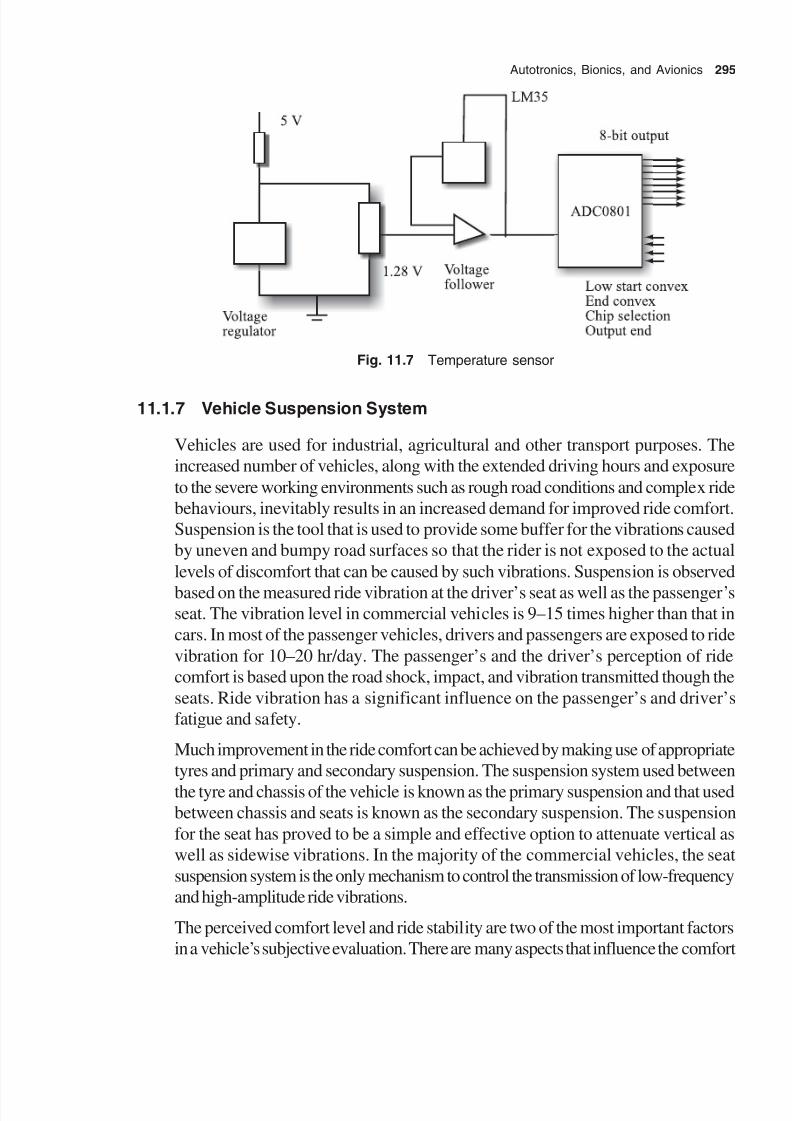
8/11/2019 Introduction to Mechatronics - Appuu Kuttan.pdf
http://slidepdf.com/reader/full/introduction-to-mechatronics-appuu-kuttanpdf 304/345
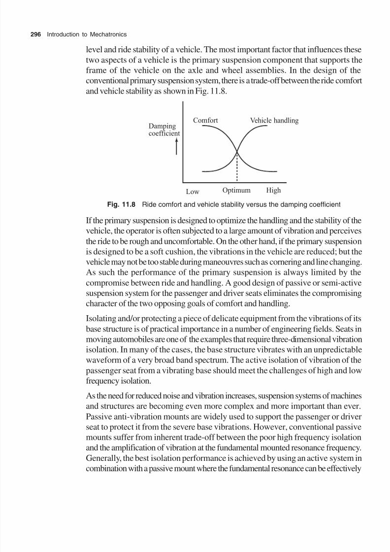
8/11/2019 Introduction to Mechatronics - Appuu Kuttan.pdf
http://slidepdf.com/reader/full/introduction-to-mechatronics-appuu-kuttanpdf 305/345
296 Introduction to Mechatronics
level and ride stability of a vehicle. The most important factor that influences these
two aspects of a vehicle is the primary suspension component that supports the
frame of the vehicle on the axle and wheel assemblies. In the design of the
conventional primary suspension system, there is a trade-off between the ride comfort
and vehicle stability as shown in Fig. 11.8.
Comfort Vehicle handling
Low Optimum High
Dampingcoefficient
Fig. 11.8 Ride comfort and vehicle stability versus the damping coefficient
If the primary suspension is designed to optimize the handling and the stability of the
vehicle, the operator is often subjected to a large amount of vibration and perceives
the ride to be rough and uncomfortable. On the other hand, if the primary suspension
is designed to be a soft cushion, the vibrations in the vehicle are reduced; but the
vehicle may not be too stable during maneouvres such as cornering and line changing.
As such the performance of the primary suspension is always limited by the
compromise between ride and handling. A good design of passive or semi-active
suspension system for the passenger and driver seats eliminates the compromisingcharacter of the two opposing goals of comfort and handling.
Isolating and/or protecting a piece of delicate equipment from the vibrations of its
base structure is of practical importance in a number of engineering fields. Seats in
moving automobiles are one of the examples that require three-dimensional vibration
isolation. In many of the cases, the base structure vibrates with an unpredictable
waveform of a very broad band spectrum. The active isolation of vibration of the
passenger seat from a vibrating base should meet the challenges of high and low
frequency isolation.
As the need for reduced noise and vibration increases, suspension systems of machines
and structures are becoming even more complex and more important than ever.
Passive anti-vibration mounts are widely used to support the passenger or driver
seat to protect it from the severe base vibrations. However, conventional passive
mounts suffer from inherent trade-off between the poor high frequency isolation
and the amplification of vibration at the fundamental mounted resonance frequency.
Generally, the best isolation performance is achieved by using an active system in
combination with a passive mount where the fundamental resonance can be effectively

8/11/2019 Introduction to Mechatronics - Appuu Kuttan.pdf
http://slidepdf.com/reader/full/introduction-to-mechatronics-appuu-kuttanpdf 306/345
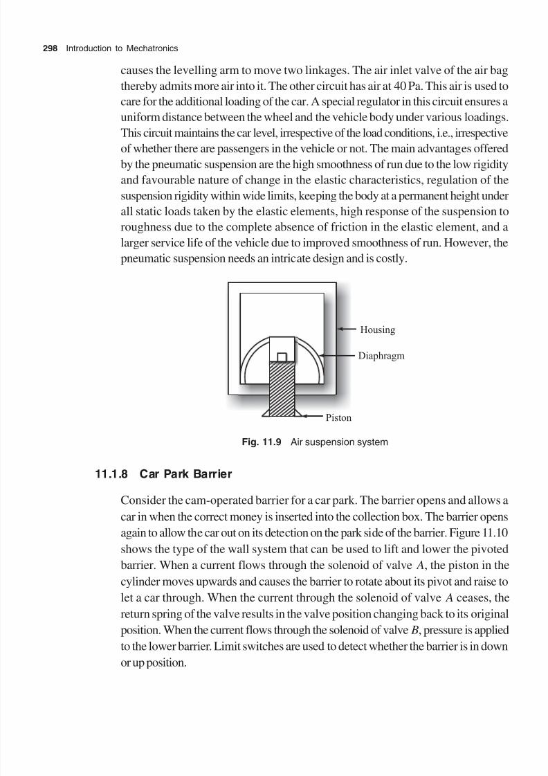
8/11/2019 Introduction to Mechatronics - Appuu Kuttan.pdf
http://slidepdf.com/reader/full/introduction-to-mechatronics-appuu-kuttanpdf 307/345
298 Introduction to Mechatronics
causes the levelling arm to move two linkages. The air inlet valve of the air bag
thereby admits more air into it. The other circuit has air at 40 Pa. This air is used to
care for the additional loading of the car. A special regulator in this circuit ensures a
uniform distance between the wheel and the vehicle body under various loadings.
This circuit maintains the car level, irrespective of the load conditions, i.e., irrespectiveof whether there are passengers in the vehicle or not. The main advantages offered
by the pneumatic suspension are the high smoothness of run due to the low rigidity
and favourable nature of change in the elastic characteristics, regulation of the
suspension rigidity within wide limits, keeping the body at a permanent height under
all static loads taken by the elastic elements, high response of the suspension to
roughness due to the complete absence of friction in the elastic element, and a
larger service life of the vehicle due to improved smoothness of run. However, the
pneumatic suspension needs an intricate design and is costly.
Housing
Diaphragm
Piston
Fig. 11.9 Air suspension system
11.1.8 Car Park Barrier
Consider the cam-operated barrier for a car park. The barrier opens and allows a
car in when the correct money is inserted into the collection box. The barrier opens
again to allow the car out on its detection on the park side of the barrier. Figure 11.10
shows the type of the wall system that can be used to lift and lower the pivoted
barrier. When a current flows through the solenoid of valve A, the piston in the
cylinder moves upwards and causes the barrier to rotate about its pivot and raise to
let a car through. When the current through the solenoid of valve A ceases, the
return spring of the valve results in the valve position changing back to its original
position. When the current flows through the solenoid of valve B, pressure is applied
to the lower barrier. Limit switches are used to detect whether the barrier is in down
or up position.

8/11/2019 Introduction to Mechatronics - Appuu Kuttan.pdf
http://slidepdf.com/reader/full/introduction-to-mechatronics-appuu-kuttanpdf 308/345

8/11/2019 Introduction to Mechatronics - Appuu Kuttan.pdf
http://slidepdf.com/reader/full/introduction-to-mechatronics-appuu-kuttanpdf 309/345
300 Introduction to Mechatronics
11.1.10 Air Bag Deployment System
A sensor and an actuator embedded in a microsystem are used to operate the air
bag deployment system in an automobile. The impact of the car in a serious collision
is felt by a micro-inertia sensor built on the principle of micro-accelerometer. The
sensor generates an appropriate signal to actuate the deployment of an air bag to
protect the driver and passengers from serious injuries due to the impact of collision.
Figure 11.11 shows a micro-inertia sensor employed for rapid deployment of an air
bag. The sensor contains two micro-accelerometers mounted onto the chassis of
the car. The accelerometer on the left measures the deceleration in the horizontal
direction and the accelerometer on the right measures the deceleration in the
transverse direction. Both these accelerometers are mounted on the same integrated
circuit chip along with a signal transducer and processing unit. The entire chip has
an approximate size of 3 mm ¥ 2 mm, with the micro-accelerometer occupyingabout 10% of the overall chip area. Accelerometers that can sense in the range of
±2 g are used in car suspension systems and antilock braking systems. Accelerometers
in the sensing range of ±50 g are used to actuate the air bag deployment. In the case
of micro-accelerometer, significant different arrangements are necessary because
very limited space is available in miniature devices. A miniature silicon beam with
attached mass constitutes a spring-mass system and the air in the surrounding space
is used to produce the damping effect. The structure that supports the mass acts as
a spring.
Signaltransduction
Sensor Actuator
Power supply
Piezocrystal
Silicon substrate
Fig. 11.11 Micro-inertia sensor air bag deployment
11.2 Bionics
Bionics is poised to have significant stake in mechatronic sensors market in the near
future. Biomedical sensors are mainly used for diagnostic analyses. Because of its
miniature size, a biomedical sensor requires less amount of sample and can produce

8/11/2019 Introduction to Mechatronics - Appuu Kuttan.pdf
http://slidepdf.com/reader/full/introduction-to-mechatronics-appuu-kuttanpdf 310/345
Autotronics, Bionics, and Avionics 301
results significantly faster. These sensors can be produced in batches, thus resulting
low unit cost of the sensor. Another cost cutting factor is that most of these sensors
are disposable, thus manual labour involving cleaning and proper treatment for reuse
is saved. Biosensors are extensively used in analytical chemistry and biomedical
care as well as genetic engineering. These sensors usually involve biological moleculessuch as antibodies or enzymes, which interact with analytes that are to be detected.
Major advantages of the use of mechatronic systems in biomedicine are as follows:
∑ Functionality for biomedical operators
∑ Adaptability to existing instruments and equipment
∑ Compatibility with biological systems
∑ Controllability, mobility, and easy navigation facilities for operators
∑ Possibility of the fabrication of mechatronic structures with a high aspect ratio
(the ratio of the depth dimension to the surface dimension of the structure)
11.2.1 Biological Systems
Of the 91 naturally occurring elements, many are found in biological systems. Traces
of metals such as zinc, iron, vanadium, manganese, selenium, and copper are used
for specific biological functions in human body. Well over 95% of the mass of plants
and animals is made of four elements: hydrogen, oxygen, nitrogen, and carbon.These are also the elements that dominate in most of the synthetic polymers. These
elements can combine (bond) in various ways to give rise to a number of simple and/
or complex biological structures. The nature has used this feature of these elements
to build various kinds of biological systems to accomplish the various life processes.
Scientists, on similar lines, have used them to make new materials.
The numerous molecules in our own body are responsible for respiration, digestion,
temperature regulation, protection, and all other functions that our body carries out.
The molecules found in nature are complex. For these molecules to perform usefulfunctions, they must be easy to assemble, recognize, and bind to other molecules.
They must also be products of biological processes and have variable properties.
There are four broad classes of biological molecules. The first three are nucleic
acids, proteins, and carbohydrates, which are all polymer structures. The fourth is
the catalytical category (enzymes) composed of particularly small molecules that
perform special tasks.

8/11/2019 Introduction to Mechatronics - Appuu Kuttan.pdf
http://slidepdf.com/reader/full/introduction-to-mechatronics-appuu-kuttanpdf 311/345
302 Introduction to Mechatronics
Proteins make up much of the bulk of biological mass. Our nails are mostly made up
of the protein keratin. Oxygen is carried in our blood by the protein haemoglobin and
the protein nitrogen is responsible for taking nitrogen out of the air. There are thousands
of proteins, most of which are very well understood in terms of their structures and
functions. However, some proteins are still a mystery as far as their structures andfunctions are concerned. Proteins are machines of biology, the functional agents
that make things happen.
Nucleic acids are of two types: ribose nucleic acid (RNA) and de-oxyribose nucleic
acid (DNA). Though both RNA and DNA are needed to make proteins, the former
(i.e., RNA) has not yet been of major interest in developing nanostructures.
The DNA consists of a sugar and side chain containing a negative charge due to the
presence of phosphorus and oxygen atoms in it. DNA molecules are stacked planar
molecules, which are on top of one another like a pile of poker chips. Each of the
stacked chips consists of two separate planar molecules held together weakly by
bridges between oxygen and nitrogen or hydrogen. Because each chip is held at
both its right and left ends and because the structure is helical, the DNA has the
structure of a double helix or double spiral staircase. It also looks like a spring when
it is tightly wound.
The DNA is an almost unique molecule because each chip can have one of the four
compositions, namely, AT, TA, CG, or GC. For each position on the strand, it is
possible to control which of the base pairs is present because the two planer molecules
that compose them can only be chosen from a set of four molecules adenine, thiamine,guanine, and cytosine (which are abbreviated A, T, G, and C). A and T will only bond
to each other and not to G and C. Similarly, G and C will only bond to each other and
not to A and T. Because of this limitation, the only possible base pairs are AT and
GC and their opposites TA and CG. These are placed on a double helix in a particular
order and it is the code for all the functions of an organism. The genetic code is
simply an arrangement of base pairs in the DNA double helix. This code is read in a
very sophisticated way by RNA and by proteins, which use the information to make
protein-based biological systems necessary for carrying out biological process of
life.
Another class of macromolecules is called polysaccharides. Polysaccharides are
simply sugars made of very large molecules. They are crucial to the functioning of
a cell. Some of these are formed in ligaments and in other biological structural
materials. However, these are not yet of major use in the synthetic material technology.
The fourth class of biological molecules consists of very small molecules. These
molecules include water and oxygen as major energy sources. Carbon dioxide is the
raw material for making plants. Nitric oxide is a very small molecule consisting of

8/11/2019 Introduction to Mechatronics - Appuu Kuttan.pdf
http://slidepdf.com/reader/full/introduction-to-mechatronics-appuu-kuttanpdf 312/345
Autotronics, Bionics, and Avionics 303
nitrogen and oxygen bonded together. It plays many roles in biology from acting as
a secondary messenger for communication or relay messenger for communication
within in a cell to causing erectile function.
There are some other molecules that are infrequent and small but still crucial in
biological systems. These include simple sugar and all drug molecules. A druggenerally works by binding itself either to a protein or to a DNA and causing changes
in the functions of the host structure/cell. Often the binding of these small molecules
is very specific and very important. The ability of one molecule to attract and bind
onto another molecule is often referred to as molecular recognition. Molecular
recognition is generally very specific. Thus, molecular recognition can be used for
sensory applications involving biological matter. Molecular recognition is one of the
key features of nanotechnology. Much of nanotechnology depends on building from
bottom-up, making molecules that can organize themselves on their own or with a
supporting surface such as a metal or plastic.
11.2.2 Biostructure
Sam Stupp, Head of the Institute of Northwestern, conducted research on human
repair, which involved utilization of self-assembly and nanostructures to repair
damaged body parts or organs. His research was focused on nanoscale biostructures
that can mimic or effect a biological process. One example of nanoscale biostructures
is the self-assembling artificial bone. The molecules that make up the bone are held
together by chemical bonds. These bonds hold the molecules together with eachother in a particular shape. The molecules in the bone are designed to occupy space
in a particular way so that they may assemble spontaneously to form a desired
shape. Once assembled, the molecules are packed closely enough for the bone to be
very strong. The structure of packed molecules can be made compatible with the
human immune system by properly choosing the head groups of the molecules. A
group of molecules ultimately forms the outer shell of the artificial bone template.
The outer shell is designed so that natural bones begin to form around it like corals
on a reef or gold on a plated jewellery. The key to human repair is by allowing the
body to fix damaged tissue naturally rather than replacing with steel or ceramicimplants.
11.2.3 Glucose Detection and DNA Sensing
Detection of glucose levels in human body is a classic case of biosensing. Diabetic
patients cannot control their insulin level if the level of blood glucose fluctuates
tremendously. If the level gets either too high or too low, their condition can be life
threatening. Currently such patients must actually draw blood on a daily basis or
8/11/2019 Introduction to Mechatronics - Appuu Kuttan.pdf
http://slidepdf.com/reader/full/introduction-to-mechatronics-appuu-kuttanpdf 313/345
304 Introduction to Mechatronics
even more often to monitor the blood glucose level. Sensing the blood glucose level
can be done in many ways, using optical, conduction, or molecular recognition
methods. None of these have yet been shown to be compatible with an implantable
simple device that could automatically show or continuously sense the glucose level
in the blood. This remains one of the major challenges in chemical sensing and
nanoscale structures.
The DNA sensing is potentially an enormous area in which the application of
nanoscience can prove to be path breaking. One can sense the structure with the
sequence GEGEAAG by using a strand GCGCAAG. This means that a single strand
of, say, six bases can contain 4096 different combinations. Consequently, a particular
biological target such as botulism or strap or scarlet always has a unique DNA
sequence. It is possible to target a short sector of the DNA sequence, say, a section
of 10–15 bases. It can be uniquely sensed without any error.
The most important application of DNA sensing will probably come in thegeneralization of a laboratory on a chip concept. By using the powerful analytic
capability of such dense micro-laboratories, it will be possible to include several
screening sensors on a chip. This chip can be used to recognize a viral or bacterial
DNA associated with several different diseases found in the body. This chip could
also be used to sense the presence of toxic species, either natural or artificial. Since
the entire human genome is known, a biochip can be used to sense either a particular
DNA signature or a particular protein signature known to be characteristic of a
disease. It is also possible to create a sensor that takes advantage of the DNA
recognition technique. The simplest DNA recognition sensor works by introducing astrand of DNA complimentary to the analyte into a solution to be tested. If the
analyte is present, it will hybridize with the test DNA and form a double strand.
Hybridization confirms that the analyte is present, or finding out that hybridization
has occurred is trivial. One cannot see the double strands without very sophisticated
instruments. Therefore, one of the great challenges in DNA sensing is to amplify
the effect of hybridization so that it is easy for measurement. One way to provide
amplification is to change the optical properties of gold or silver nanodots that are
attached to the DNA. The change in the colour of gold upon changing the size of the
gold cluster and the molecular recognition is called quantum optical effect. Thecolour change is measured by a device called calorimetric sensor, which can be
read by simply looking at it. Nanosphere lithography is used to prepare the tiny gold
dots on a surface. A sensor is designed to recognize a particular portion of the
analyte appearing in the solution. If one wants to construct an explosive detection
sensor, the problem is much more complex. Nitrates, which are common to most
explosives, are common in household items including fertilizers. If one detects them
to an accuracy of a single molecule, then even fertilizers are carrying a bomb. A
great deal of research is underway in this direction.
8/11/2019 Introduction to Mechatronics - Appuu Kuttan.pdf
http://slidepdf.com/reader/full/introduction-to-mechatronics-appuu-kuttanpdf 314/345
Autotronics, Bionics, and Avionics 305
11.2.4 Drug Delivery
The size of the human body is very large compared to the size of a molecule. It is
important for the thermofusion effectiveness that drug molecules find/reach the
place in the body where they are needed/effective. Bio-availability refers to the
presence of drug molecules where they are needed in the body and where they willdo the most good. The issue of drug delivery aims at maximizing bio-availability both
over a period of time and at the specific place in the body. Increasing the bio-
availability is seldom as simple as increasing the amount of drug used. The drugs
used in chemotherapy are actually somewhat toxic and need to be target-specific to
avoid damage to the normal/healthy tissue. It is necessary to keep the drug doses to
a minimum, otherwise the amount used can adversely affect or even kill a patient.
Taking these issues into account, drug delivery assumes a lot of significance.
Nanotechnology and nanoscience are very useful in developing entirely new ways
for increasing bio-availability and improving the drug delivery.Magnetic nanoparticles used for computer memory can be used for drug delivery
also. For drug delivery, the molecular recognition method is used to bind a nanomagnet
to the drug to be delivered. External control is exercised over the magnetic field
created by magnetic nanoparticles to improve local bio-availability of the drug.
Effectively, a doctor can drag drug molecules through the body in the same way as
you drag an iron filing across a table with a hand magnet. One interesting combination
of smart materials and drug delivery is the triggered response. This consists of
placing drug molecules within the body in an inactive form that works upon
encountering a particular signal. A simple example is antacid implored in a coating
of a polymer that dissolves in a highly acidic spot. The antacid is released only when
the outer polymer coat encounters a highly acidic spot in the digestive track.
11.2.5 Photodynamic Therapy
In photodynamic therapy, a particle is placed within the patient’s body. This particle
is illuminated with a light source from outside of the body. The light may come from
outside from a laser or light bulb. The light is absorbed by the particle, after which
several things might happen. If the particle is simply a metal nanodot, the energy
from the light will heat the dot, which, in turn, will heat any tissue within itsneighbourhood. With the same particular molecular dot, light can also be used to
produce highly energetic oxygen molecules. Such oxygen molecules are very reactive
and will chemically react with (and, therefore, destroy) many organic molecules that
are next to them.
The photodynamic therapy is attractive for many reasons. One reason is that, unlike
the traditional chemotherapy, it is directed at the damaged/diseased cell. The
chemically reactive excited oxygen or quantum data is released only where such
cells are present and where the light is illuminated. This ensures that, unlike the

8/11/2019 Introduction to Mechatronics - Appuu Kuttan.pdf
http://slidepdf.com/reader/full/introduction-to-mechatronics-appuu-kuttanpdf 315/345
306 Introduction to Mechatronics
traditional chemotherapy, the photodynamic therapy does not leave a fixed trail of
highly aggressive and reactive molecules throughout the body.
11.2.6 Molecular Motors
Molecular motors are proteins or protein complexes that transform chemical energy
into mechanical energy at a molecular level scale. These are responsible for producing
and transducing the energy stored in ATP, which is the common energy currency of
the body for powering every process and action. The sodium/potassium, called ATP
molecule, actually acts as a rotary motor. A critical amount of the nanostructure
rotates around a pivot and the outside part of the nanostructure reacts differently
with the chemical group around the periphery. This rotary motor is one of the several
molecular motor mechanisms that are now understood to play important roles in the
functional biology of a cell. Molecular motors also allow us to manage the availabilityof the different components of the cell as they move about within the cellular structure.
Kinesin is a nanoscale molecular motor that carries molecular cargo through the cell
by moving along nanoscale tracks, called microtubes, within the cell. In many respects,
it is the “world’s smallest type of train”. Molecular motion is also responsible for
signal transduction in the human ear. Molecular motion may provide acceleration
and motional energy for both artificial nanostructures within the body and in more
complex nanostructure assemblies.
11.2.7 Neuro-electronic Interface
The neuro-electronic interface involves the idea of constructing nanodevices that
can permit computers to be joined and linked to the neurosystem. The construction
of a neuro-electronic interface system requires the building of a molecular structure
that will permit control and detection of nerve impulses by an external computer.
The real challenge is to combine computational technology and bio-nanotechnology.
The nerves in the human body convey messages by permitting electrical current to
flow between the brain and nerve centre throughout the body. The most important
ions for signals are sodium and potassium ions. These ions move along sheets andchannels that have evolved specially to permit special, controllable, rapid ion motion.
This is the mechanism that allows you to feel sensation. For example, when you put
your foot in hot water, a signal is transmitted by the local nerve through the nervous
system to the brain. The brain interprets the transmitted signal and processes it for
a suitable reaction. Often this process results in a response being filtered into the
muscular system. The aim of the neuro-electronic interface technology is to permit
the registration and interpretation of these signals as well as response to them to be

8/11/2019 Introduction to Mechatronics - Appuu Kuttan.pdf
http://slidepdf.com/reader/full/introduction-to-mechatronics-appuu-kuttanpdf 316/345
Autotronics, Bionics, and Avionics 307
handled by a computer. The sensor must be able to sense ionic currents and cause
current to flow backward so that the muscular system can be instructed to perform
a desired motion. The most obvious structure will be a molecular conductor or
molecule whose own conduction process, ions, or electrons can link with the ionic
motion in a nerve fibre.
11.2.8 Electrochemical Sensor
The electrochemical sensor works on the principle that certain biological substances,
e.g., glucose in human blood, can release certain element(s) by chemical reactions.
These substances can alter the pulse flow pattern in a sensor, which can be readily
detected. Figure 11.12 illustrates the working principle of a biomedical glucose
detector. A small sample of blood is introduced to a sensor with a polyvinyl alcohol
solution. Two electrodes are present in the sensor. A thin sheet of platinum and athin Ag/AgCl film are used as the reference electrodes. The following chemical
reaction takes place between the glucose in the blood sample and the oxygen in the
polyvinyl alcohol solution:
VoltageH molecules+
Ptelectrode
Ag/AgClelectrode
Blood sample
Fig. 11.12 Biomedical glucose detector
Glucose + O2 = gluconolacton + H2 O2
The H2O2 produced in the chemical reaction is electrolysed by applying a potential
to the platinum electrode. This results in the production of positive hydrogen ions,which flow towards the electrodes. The glucose concentration in the blood sample
is thus measured by measuring the current flow between the electrodes.
11.2.9 Biotechnology
Mechatronics plays an important role in biotechnology even though it is a small
subdomain of biotechnology. Biotechnology includes all techniques that use living
organisms or substances obtained from them to make or modify a product. It involves

8/11/2019 Introduction to Mechatronics - Appuu Kuttan.pdf
http://slidepdf.com/reader/full/introduction-to-mechatronics-appuu-kuttanpdf 317/345
308 Introduction to Mechatronics
improvement of microbe, plant, and animal species. Genes and gene products are
the basic tools in biotechnology. Biotechnology aims at harnessing the genetic diversity
in the living organisms for the benefit of the humankind. Understanding of genes and
the possibility to manipulate them are the very bases of modern biotechnology. Classical
genes and manipulation of the genes at cellular level have played a major role inenhancing the productivity of crops, plants, and animals. Molecular manipulation of
genes to obtain better products requires input from specialists in many different
areas of biology, besides from specialist in other branches of science, especially
mechatronics.
The splendors of biotechnology are so much that it almost seems to be the science
of wish fulfillment. Bigger fruits, bright flowers, higher yields, super cattle, exotic
colours and flavours, cheaper medicines, and more efficient vaccines are the products
of biotechnology.
The first studies of genetic engineering have been reported on microbes. Bacteria in
the soil that digest animal waste or even burial carcasses are an example of genetic
engineering involving microbes. Imagine bacteria that would be able to digest petrol
or crude oil. Such bacteria could be used for clean-up operations when oil tankers
spill substances of the crude oil in the sea. Just releasing such bugs at the spillage
area would help the mopping-up operations. They could eat off the oil and multiply
progressively to do more of the same. This method would be much cheaper, fair, and
more convenient than other alternatives.
Agriculture started in Europe about 10000 BC. New plants were brought byagriculturists from one country to other for cultivation and consumption across the
world. The rose plant was brought by a British ambassador to the Moghul court and
gifted to the empress Noorjahan. She arranged for the propagation of the rose
flower in India some 400 years ago. Many of the vegetables that we eat in India
were imported from other countries. For example, potato is a native of South America.
It was exported to other countries of the world from there. Potato was brought from
South America to Europe in 1570 and to India around the eighteenth century. People
started cultivating potatoes in India from early eighteenth century onwards.
The choice of potato seeds for planting is largely influenced by its size, shape, colour,
and tastes, skin appearances, storing capabilities, and processing properties. A potato
has to be high in solid or dry matter in order to be considered suitable for making
good potato chips. Researchers at Monsanto Company in the USA have inserted a
starch-producing gene from the common intestinal bacterium that can make potato
20% more starch rich than the best potato in the market. Genetic engineering has
yielded superpotatoes. Calgene Pacific, a Melbourne based biotechnology company,
has announced that it has isolated a gene that is capable of providing twice the
8/11/2019 Introduction to Mechatronics - Appuu Kuttan.pdf
http://slidepdf.com/reader/full/introduction-to-mechatronics-appuu-kuttanpdf 318/345
Autotronics, Bionics, and Avionics 309
normal number of tubers. This new variety of potato is termed superpotato. This has
helped growers to double potato yield per hectare. The company also claims that
cultivation of superpotato provides more nutrition from less land and in less time
than rice, wheat, or corn. Potatoes are cultivated in 130 countries in the world. An
increase in the yield of potato has considerable impact on the potato production theworld over. Biotechnology facilitates incorporating borrow genes from other organisms
into a target species. The greater wax moth has a protein that stores large amounts
of tyrosine. This protein is the product of a moth gene. If this gene is incorporated
into potato, the gene might change tyrosine location and form with tuber cells. That
might make tyrosine less accessible to the blacking enzyme in the potato.
11.3 Avionics
Considerable effort and progress have been made in recent years in the developmentof mechatronic systems in the aerospace industry. Numerous and complex
mechatronic systems are used in advanced commercial and military aircrafts. With
the ever-increasing emphasis on robustness and safety, there is a trend towards
using more mechatronic systems in aerospace industry. This has given rise to a new
area of mechatronics in the form of avionics. The major applications of mechatronic
systems in aerospace industry can be classified as follows:
∑ Cockpit instrumentation
∑ Safety devices
∑ Wind tunnel instrumentation
∑ Sensors for fuel efficiency and safety
∑ Microgyroscope for navigation and stability
∑ Microsatellites
11.3.1 Cockpit Instrumentation
Air-data systems vary in complexity from a light airplane to advanced commercial
or military aircrafts. However, all air-data computations are based upon four sensed
parameters, namely, static pressure, total pressure, temperature, and the angle of
attack. Pressure and temperature of the atmosphere are functions of the altitude
above the sea level, latitude, season, and time of day. Static pressure can be easily
and accurately measured because the actual altitude for a given pressure varies
only slowly with respect to time and distance.
A Pitot tube is a pressure measuring instrument used to measure fluid flow velocity
and, more specifically, to determine the airspeed of an aircraft. The Pitot tube is

8/11/2019 Introduction to Mechatronics - Appuu Kuttan.pdf
http://slidepdf.com/reader/full/introduction-to-mechatronics-appuu-kuttanpdf 319/345
310 Introduction to Mechatronics
named after its inventor, Italian born French engineer Henri Pitot. The opening on
the smooth side of the Pitot-static tube provides a source of the atmospheric pressure,
termed static pressure. The open end of the Pitot-static tube is headed into the
stream and provides a source of the total pressure resulting from the impact of a
body travelling through the atmosphere. The difference between the total pressure
and the static pressure gives the dynamic force, which contains the velocity term.
The speed of the aircraft can thus be determined. Most of the Pitot-static tubes are
electrically heated to melt off any ice that might form. Otherwise, ice might partly or
completely seal off the opening and the instrument will give erroneous results.
Most of the aircraft altimeters operate like the aneroid barometer, except that
altimeters are calibrated in height instead of pressure. Static pressure surrounding
one or more evacuated diaphragm capsules operates a pointer through a system of
linkages and gears. Corrections must be made for changes in the barometer pressure.
A sensitive altimeter shows changes in pressure for an altitude of 2 m or less. Sinceatmospheric pressure reduces to half for approximately every 6000 m increase in
altitude, non-linear diaphragm linkage systems are used to provide a complete altitude
range. Pressure altitude information may be supplied by air-data computers to various
forms of indicator and display systems.
Air-speed indicators work on the principle that the difference between the total
pressure and the static pressure is the measure of the indicated air speed. The
indicated air speed at which a given aircraft with a given load stalls is a constant
over a wide range of pressure and temperature. The knowledge of this is of utmost
importance during take-off and landing as also during flight. The true air speed isprimarily useful in navigation. This factor is a function of not only the difference
between the total and static pressures but also temperature. A temperature indicator
is in effect a computer that operates on a complex relationship of two pressure
measurements and the air temperature measurement to give the correct indication.
A rate climb indicator comprises an enclosed volume of air connected to the
atmospheric pressure through constriction. As the altitude changes, the enclosed
pressure lags the outside pressure. The pressure difference is measured in terms of
the rate of change of altitude or the rate of climb. Since any change in temperature
causes a proportional change in pressure of an enclosed volume of the air, theinstrument enclosure must be a good thermal insulator to prevent all but very gradual
temperature changes of the enclosed air. Otherwise, correction must be introduced
for both static pressure and temperature to provide the correct rate of climb
information.
The angle of attack transducer measures the acute angle between the velocity
vector of the aircraft through the surrounding air and some reference such as the
force-opt axis of the aircraft or the chord of an aircraft. The lift developed by an
aircraft wing increases as a function of the angle of attack and the airplane velocity.

8/11/2019 Introduction to Mechatronics - Appuu Kuttan.pdf
http://slidepdf.com/reader/full/introduction-to-mechatronics-appuu-kuttanpdf 320/345
8/11/2019 Introduction to Mechatronics - Appuu Kuttan.pdf
http://slidepdf.com/reader/full/introduction-to-mechatronics-appuu-kuttanpdf 321/345
312 Introduction to Mechatronics
need periodic, scheduled check, because the equipment does not function except in
case of emergency. Most alarm installations are of audiovisual type, with illuminated
name plates or bull-eye lights. There is a means to silence the alarm and switch the
light to steady state. Another push button usually is provided for testing other
components of the system.
Micro-accelerometers or micro-inertial sensors are used to eject the pilot seat from
the aircraft, especially in military airplanes. The use of the seat eject system protects
the pilot in the event of an emergency. The sensor opens the latch where the seat is
loaded with a spring, which throws the seat along with the pilot a distance away
from the aircraft. When it is detached from the aircraft, a parachute automatically
opens to ensure safe landing of the pilot.
11.3.3 Aircraft Guidance and Control
To guide and control an aerospace vehicle successfully is a matter of measuring
position, determining path errors, and controlling to correct the path. These three
functions usually are called navigation, guidance, steering, and control. Navigation
determines the position, guidance determines the error from the indicated path, steering
is used to select a proper series of changes in the path, and control changes the
forces on the vehicle to adjust them with the direct path changes. Initial guidance
predicts the ballistic path. The aircraft guiding system measures accelerator and
recalls the reference angle, computes velocity and position, predicts the destination,
determines a preferred path to correct the error and controls the forces to change
the path from steering instructions, all can be automated. Aerospace vehicle systems
have many degrees of automation. Almost all aerospace vehicle systems use
combinations of all or many of automatic, manual, remote, self-contained, and
preprogrammed corrections.
Aerospace vehicles may be piloted by a human being or an automatic flight control
system. Gyroscope instruments are among the most important elements of the flight
instrumentation and control systems whether for assisting a human pilot or for
providing input to a fully automatic flight control system. A wide variety of gyroscopeinstruments are used in aircrafts. The rate gyroscope is a device designed to measure
the instantaneous angular velocity component of a body with respect to the inertial
space. Its typical applications include autopilot damping, rate of turn indicator, limiting
antenna stabilization, and telemetry instrumentation. The rate integrating gyroscope
or floated gyroscope can be designed as either a single- or two-axis device. It is
designed so that the fluid damping between gimbals and housing is the predominant
torque, which balances the input rate precessional torque. Figure 11.13 illustrates
the working principle of a gyroscope.
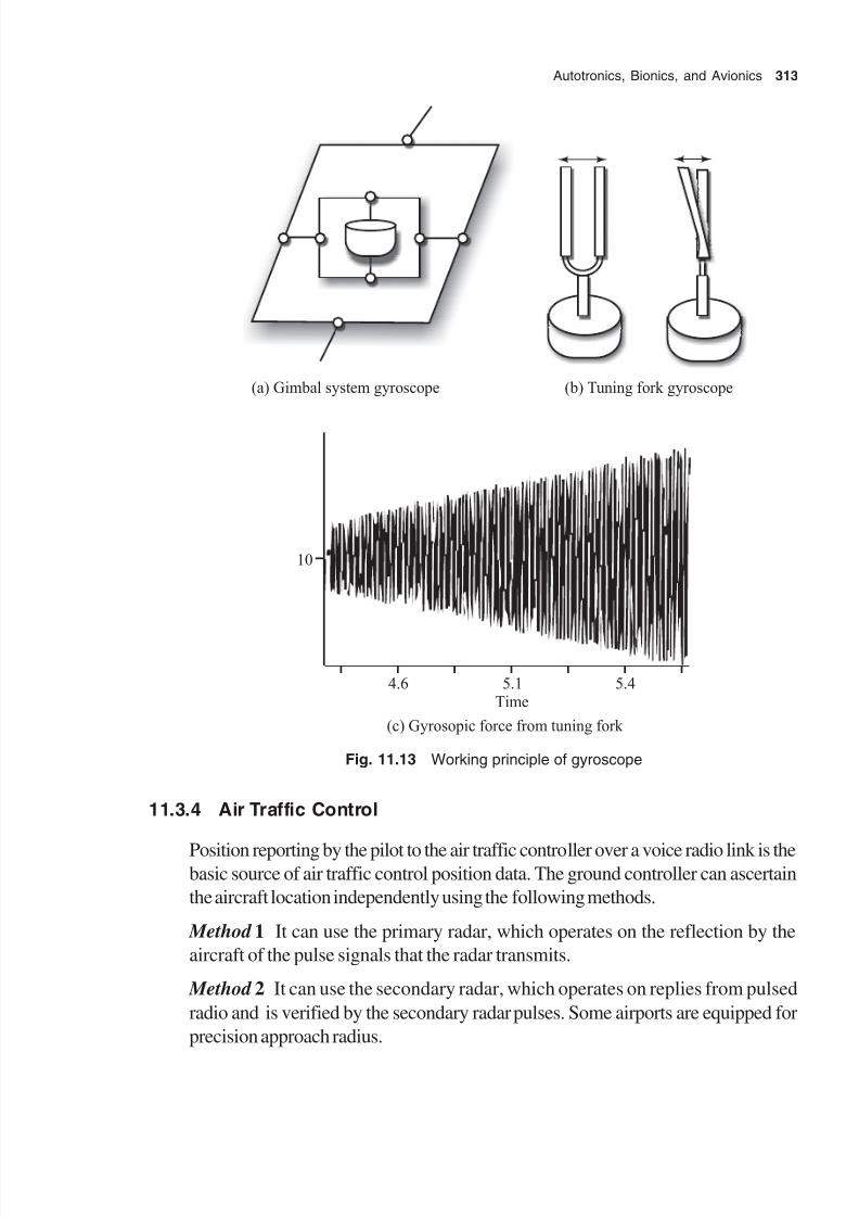
8/11/2019 Introduction to Mechatronics - Appuu Kuttan.pdf
http://slidepdf.com/reader/full/introduction-to-mechatronics-appuu-kuttanpdf 322/345
Autotronics, Bionics, and Avionics 313
(a) Gimbal system gyroscope (b) Tuning fork gyroscope
10
4.6 5.1 5.4Time
(c) Gyrosopic force from tuning fork
Fig. 11.13 Working principle of gyroscope
11.3.4 Air Traffic Control
Position reporting by the pilot to the air traffic controller over a voice radio link is thebasic source of air traffic control position data. The ground controller can ascertain
the aircraft location independently using the following methods.
Method 1 It can use the primary radar, which operates on the reflection by the
aircraft of the pulse signals that the radar transmits.
Method 2 It can use the secondary radar, which operates on replies from pulsed
radio and is verified by the secondary radar pulses. Some airports are equipped for
precision approach radius.
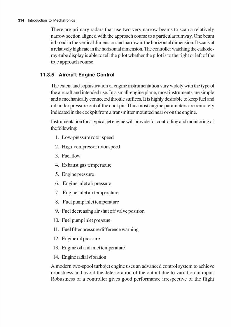
8/11/2019 Introduction to Mechatronics - Appuu Kuttan.pdf
http://slidepdf.com/reader/full/introduction-to-mechatronics-appuu-kuttanpdf 323/345
314 Introduction to Mechatronics
There are primary radars that use two very narrow beams to scan a relatively
narrow section aligned with the approach course to a particular runway. One beam
is broad in the vertical dimension and narrow in the horizontal dimension. It scans at
a relatively high rate in the horizontal dimension. The controller watching the cathode-
ray-tube display is able to tell the pilot whether the pilot is to the right or left of thetrue approach course.
11.3.5 Aircraft Engine Control
The extent and sophistication of engine instrumentation vary widely with the type of
the aircraft and intended use. In a small-engine plane, most instruments are simple
and a mechanically connected throttle suffices. It is highly desirable to keep fuel and
oil under pressure out of the cockpit. Thus most engine parameters are remotely
indicated in the cockpit from a transmitter mounted near or on the engine.Instrumentation for a typical jet engine will provide for controlling and monitoring of
the following:
1. Low-pressure rotor speed
2. High-compressor rotor speed
3. Fuel flow
4. Exhaust gas temperature
5. Engine pressure
6. Engine inlet air pressure
7. Engine inlet air temperature
8. Fuel pump inlet temperature
9. Fuel decreasing air shut off valve position
10. Fuel pump inlet pressure
11. Fuel filter pressure difference warning
12. Engine oil pressure
13. Engine oil and inlet temperature
14. Engine radial vibration
A modern two-spool turbojet engine uses an advanced control system to achieve
robustness and avoid the deterioration of the output due to variation in input.
Robustness of a controller gives good performance irrespective of the flight
8/11/2019 Introduction to Mechatronics - Appuu Kuttan.pdf
http://slidepdf.com/reader/full/introduction-to-mechatronics-appuu-kuttanpdf 324/345
Autotronics, Bionics, and Avionics 315
parameters such as flying at different speeds and altitudes. A jet engine receives
three inputs, namely, fuel flow, variable nozzle area, and inlet compressor vane angle
variation. Five outputs of the jet engine are required for controlling the jet. These are
∑ low-pressure turbine speed,
∑ high-pressure turbine speed,
∑ combustion chamber pressure,
∑ combustion chamber temperature, and
∑ exit input temperature of high-speed turbine.
It is noted that the low-pressure turbine work is used to run the low-pressure
compressor and the high-pressure turbine is used to run the high-pressure compressor.
The primary aim of the control system is to control the engine through regulating the
compressor surge margin. Since aero-engines are highly non-linear system, it isnormal for several controllers to be designed at different operating points and scheduled
across the flight envelop. Also in an aero-engine, there are a number of parameters,
apart from the ones being primarily controlled, that are to be kept within specified
safety limits, for example, the turbine blade temperature.
1
3
45
2
Nozzle
Fuel1: Low-pressure compressor 2: High-pressure compressor 3: Combustion chamber 4: High-pressure turbine5: Low-pressure turbine
Fig. 11.14 Schematic diagram of a high-performance gas turbine engine
The number of parameters to be controlled and/or limited exceeds the number of
controllable inputs. All the parameters cannot be controlled independently at the
same time. This problem can be tackled by designing a number of scheduled controllers,
each for a different set of output variables. For making aircraft, a robust multivariable
controller is used to provide satisfactory performance over the entire operation range
of the engine. Figure 11.14 shows the schematic diagram of a high-performance gas

8/11/2019 Introduction to Mechatronics - Appuu Kuttan.pdf
http://slidepdf.com/reader/full/introduction-to-mechatronics-appuu-kuttanpdf 325/345
316 Introduction to Mechatronics
turbine engine used for modern military aircraft. The engine has two compressors
and two turbines. The efficiency of the engine and the thrust produced depend on
the pressure ratio generated by the two compressors.
Exercises11.1 Identify the different mechatronic systems used in automobiles.
11.2 How are automobile engines managed using mechatronic systems?
11.3 Differentiate between passive, semi-active, and active vibration-suppressing
systems used in vehicles.
11.4 What is a nanostructure? Give examples.
11.5 What is a molecular motor?
11.6 What is a neuro-electronic interface? What is its future potential?
11.7 Explain the principle of photodynamics.
11.8 What is hybridization?
11.9 Enumerate different mechatronic system instruments used in aircrafts.
11.10 What are the challenges faced in controls of a two-shaft turbojet engine?
11.11 Explain the functions of an air traffic controller.

8/11/2019 Introduction to Mechatronics - Appuu Kuttan.pdf
http://slidepdf.com/reader/full/introduction-to-mechatronics-appuu-kuttanpdf 326/345
Laplace Transform
Time domain function Laplace transform
1 d (t ), unit pulse input 1
2 x (t ), unit step input1
s
3 tx (t ), unit ramp input12
s
4 t 2 x (t ), unit parabolic input
13
s
5 t n x (t ), n = 1, 2, 3, 4, ... sn!/(n + 1)
61
p t
1
s
7 22
t
x t ( )
1
3s
8 e–at
1
s a+
9 be–at b
s a+
10 te–at
12
( )s a+
11 t w
e–at
n
s a n( )+ + 1
121
1a
e at
( )- -
1
s s a( )+

8/11/2019 Introduction to Mechatronics - Appuu Kuttan.pdf
http://slidepdf.com/reader/full/introduction-to-mechatronics-appuu-kuttanpdf 327/345
318 Appendix
13 e–at – e
–bt b a
s a s b
-
+ +( ) ( )
141
ab
e
a b a
e
a a b
at bt
-
-
-
-
- -
( ) ( )
1
s s a s b( )( )+ +
15 (1 – at )e–at
s
s a( )+2
16 sin(wnt )w
w
02 2
s n+
17 sin(wnt + q)s
s
n
n
sin cosq w q
w
+
+2 2
18 cos(wnt )s
s n2 2
+ w
19 e–at sin(wnt )w
w
n
ns a( )+ +2 2
20 e–at cos(wnt )s a
s a n
+
+ +( )2 2w
211
1
1
12
2 1-
-
- +
- -
z w z z zw
e t nt nsin cos w
zw w
n
n ns s s
2
2 22( )+ +
22
w
z w z zw n t
ne t n
1
12
2
-
-
-
sin w
zw w
n
n ns s
2
2 22+ +
231
1
12
2
2 1-
-
- +
- -
w
z w z z zw n t
ne t n sin cos s
s s
n
n n
w
zw w
2
2 22+ +
∑ a, b are constants.
∑ w n is the natural frequency of the system.
∑ z is the damping ratio.

8/11/2019 Introduction to Mechatronics - Appuu Kuttan.pdf
http://slidepdf.com/reader/full/introduction-to-mechatronics-appuu-kuttanpdf 328/345
Bibliography
Textbooks
Aditya, P. Mathur (1987), Introduction to Microprocessor , Tata McGraw Hill,
New Delhi.
Bayle, H.P. (1997), Transducer Handbook , Newman Publication, USA.
Bolton, W. (1996), Instrumentation and Measurement , Newman Publication, USA.
Bolton, W. (1997), Pneumatic and Hydraulic Systems, Butterworth Heinemann,
London.
Bolton, W. (2003), Mechatronics, Pearson Education, India.Bolton, W. (2003), Programmable Logic Controller , Newman Publication, USA.
Brodley, B.A., et al. (1991), Mechatronics: Electronics in Products and Processes,
Chapman and Hall, London.
Buerk, D.G. (1993), Biosensor: Theory and Applications, Technomic Publication,
USA.
Chiltan, J.A. and M.T. Goosy (1995), Special Polymers for Electronics and
Optoelectronics, Chapman and Hall, London
Chong, E.K.P. and S.H. Zak (1996), An Introduction to Optimization, John Wiley
& Sons, USA.
Colleib, I.M. (1974), Electronics Motors and Control Techniques, TAB Books,
McGraw Hill, New York.
Croser, P. (1989), Pneumatics: Basic Level, Festo Didactic, Germany.
Dauglas, M. Considine (1991), Encyclopedia of Instrumental Control, McGraw
Hill, New York.

8/11/2019 Introduction to Mechatronics - Appuu Kuttan.pdf
http://slidepdf.com/reader/full/introduction-to-mechatronics-appuu-kuttanpdf 329/345
Bibliography 321
David, D. Gold, Berg (2000),Genetic Algorithms, Pearson Education Asia, India.
De Silva, C.W. (1989), Control Sensors and Actuators, Prentice Hall Inc.,
Englewood Cliffs, New Jersey.
Del Toro, V. (1986), Electrical Engineering Fundamentals, Prentice Hall Inc.,
Englewood Cliffs, New Jersey.
Denny, K. Mia (1993), Mechatronics, Springer Verlag, New York.
Denton, T. (1995), Automobile Electrical and Electronics Systems, Arnold
Publication, London.
Doebelin, E. (1998), System Dynamics, Marcell Dekkar Inc., New York.
Douglas, V. Hall (1987), Microprocessor and Interfacing, Programming and
Hardware, Tata McGraw Hill, New Delhi.
Dubey, G.K. (1995) , Fundamentals of Electrical Drives, Narosa Publishing House,
New Delhi.
Groover, M.P. et al. (1998), Industrial Robotics Technology: Programming and
Applications, McGraw Hill, New York.
Gaonkar, (1991), Microprocessor Architecture: Programming and Application,
Wiley Eastern, USA.
Gene, H. Hsteller, Clemand J. Savant, and Raymond J. Stefa (1982), Design of
Feedback Control Systems, Holt Saunders International Education, USA.
Gibbs, D. (1982), CNC Part Programming: A Practical Guide, Casse Publication,
London.
Harry, L. Stiltz (1969) , Aerospace Telemetry, Prentice Hall Inc., Englewood Cliffs,
New Jersey.
Hartley, J. (1984), FMS: A Tutorial Work , IFS Publication, London.
Karunakarans, et. al. (1995), HMT Handbook , Mechatronics, Tata McGraw Hill,
New Delhi.
Jain, R.K. (1997), Engineering Metrology, Khanna Publication, New Delhi.
James Reghg, A. and Henry W. Kraebber (2001), Computer Integrated
Manufacturing, Pearson Education Asia, India.
James Garratt, (1991), Design and Technology, Cambridge University Press,
Cambridge.

8/11/2019 Introduction to Mechatronics - Appuu Kuttan.pdf
http://slidepdf.com/reader/full/introduction-to-mechatronics-appuu-kuttanpdf 330/345
322 Bibliography
Hancock, John C. (1991), Introduction to Principles of Communication Theory,
Tata McGraw Hill, New Delhi.
Kalisi, H.S. (1995), Electronics Instrumentation,Technical Education Series, Tata
McGraw Hill, New Delhi.
Kamerichy, I. (1974), Heat Treatment Handbook , MIS Publications, London.
Kasop, S.O. (1997), Principles of Electrical and Engineering Materials and
Devices, Irwin Publication, USA.
Ogata, Katsahiko (2002), Modern Control Engineering, Pearson Education Asia,
India.
Krishnaswamy, K. (2003), Industrial Instrumentation, New Age International,
India.
Kurk, H.L. (1997), Electronic Materials, PWS Publication, Boston.
Lenz, J.E. (2002), Flexible Manufacturing, Marcel Dekkar Inc., New York.
Mahalik, N.P. (2005), Mechatronics: Principles, Concept and Applications, Tata
McGraw Hill, New Delhi.
Ratner, Mark and Daneil Ratner (2003), Nanotechnology, Pearson Education Asia,
India.
Mattershead, A. (1971), Electronic Devices and Circuits, Prentice-Hall of India,
New Delhi.
Meanie, Mitchel (1998), An Introduction to Genetic Algorithm, Prentice-Hall of
India, New Delhi.
Merkle, B. and M. Thomas Schrador (1990), Hydraulic Basic Level, Festo Didactic,
Germany.
Groover, Mikell P. (2001) , Automation, Production Systems and Computer
Integrated Manufacturing, Pearson Education Asia, India.
Groover, Mikell P. and Emarry W. Zimmer (1981), CAD/CAM Computer Aided Design and Manufacturing, Prentice-Hall of India, New Delhi.
Groover, Mikell P., Mckehell Weiss, Roger N. Nagal, and Nichoas G. Groover (1988),
Industrial Robotics: Technology, Programming and Applications,
McGraw Hill, New York.
Millmann, J. and C.C. Halekis (1982), Electronic Devices and Circuits, McGraw
Hill, New York.
8/11/2019 Introduction to Mechatronics - Appuu Kuttan.pdf
http://slidepdf.com/reader/full/introduction-to-mechatronics-appuu-kuttanpdf 331/345
Bibliography 323
Morrise, W. (1974), Advanced Industrial Electronics, McGraw Hill, New York.
Neelm Kavl, F. (1987), Computer Simulation and Modeling, John Wiley & Sons,
USA.
Nessulescu, Dan (2002), Mechatronics, Pearson Education Asia, India.
Nils, J. Nilson (1990) , Principle of Artificial Intelligence, Narosa Publishing House,
New Delhi.
Ogaa, K. (1997), System Dynamics, Prentice-Hall Inc., Englewood Cliffs, New
Jersey.
Pittman, J.B. (1993), Design with PLC Micro-controller , Prentice-Hall Inc.,
Englewood Cliffs, New Jersey.
Pinchar, M.J. and B.J. Callear (1996), Power Pneumatics, Prentice-Hall Inc.,
Englewood Cliffs, New Jersey.
Rafiquzaman, M. (1992), Microprocessor , Prentice-Hall Inc., Englewood Cliffs,
New Jersey.
Rahne, P. (1996), Automation with Programmable Logic Controller , Macmillan,
USA.
Rao, V. and H. Rao (1995), C++ Neural Network and Fuzzy Logic, MIS Press,
India.
Reeves, C.R. (1993), Modern Heuristic Techniques for CombinatorialOptimization, John Wiley & Sons, USA.
Rohner, P. (1996), Automation with Programmable Logic Controller , Macmillan ,
USA.
Rohner, P. and G. Smith (1990), Pneumatics Control for Industrial Automation,
Wiley Publication, USA.
Ross, Timothy J. (1995), Fuzzy Logic with Engineering Applications, McGraw
Hill, New York.
Saatyg, T. (1980), The Analytic Hierarchy Process, McGraw Hill, New York
Stadler, W. (1995), Analytical Robotics and Mechatronics, McGraw Hill, New
York.
Tai Ran Hsu (2002), MEMS and Microsystems Design and Manufacturing, Tata
McGraw Hill, New Delhi.
Tomasi, W. (1996), Advanced Electronic Communication Systems, Prentice Hall
Inc., Englewood Cliffs, New Jersey.
8/11/2019 Introduction to Mechatronics - Appuu Kuttan.pdf
http://slidepdf.com/reader/full/introduction-to-mechatronics-appuu-kuttanpdf 332/345
324 Bibliography
Warnock, I.G. (1988), Programmable Controllers: Operation and Application,
Prentice Hall Inc., Englewood Cliffs, New Jersey.
Journal papers
Angell, J.B., S.C. Terry, and P.W. Barth (1983), ‘Silicon micro-mechanical devices’,
Journal of Scientific American, vol. 248, pp. 44–53.
Askin, R.G., H.M. Selin, and A.J. Vakhari (1997), ‘A methodology for designing
flexible cellular manufacturing systems’, IEEE Transactions, vol. 29, pp.
599–895.
Bart, S.F., L.S. Tavrow, Mehregang, and M.L. Lang, ‘Micro-fabricated electro-
hydrodynamic pumps’, Journal of Sensors and Actuators, vol. 21,
pp. 193–97.
Berardinis, L.A. (1990), ‘Mechatronics: A new design strategy’, IEEE Transactions
on Mechatronics, vol. 62, pp. 1–58.
Boothroyd, G.P. and Dewuhurst (1998), ‘Product design and manufacture and
assembly’, Journal of Manufacturing Engineering, vol. 41, pp. 42–46.
Buzacott, J.A. and D.D. Yao (1997), ‘Flexible manufacturing systems: A review of
analytical models’, Journal of Management Science, vol. 36, pp. 1239–57.
Cellier, F. and H. Elonquest (1993), ‘Automated formula manipulator supports object
oriented continuous system modeling’, IEEE transactions on ControlSystems, vol. 27, pp. 28–38.
Chen, C.D., J. Shi-Shang, and A.Y. Tsen (1997), ‘Semi-continuous copolymer
composition distribution predictive control using a double ANN model
structure’, Journal of Chinese Institute of Chemical Engineers, vol. 28,
pp. 49–50.
Choi, I.H. and K.D. Wise (1986), ‘A silicon thermopile based infrared sensing array
for use in automated manufacturing’, IEEE Transactions, Electronic
Devices, vol. 31, pp. 77–79.Fan, L.S, Y.C. Jai, and R.S. Muller (1998), ‘IC processes for electrostatic micro-
motors’, IEEE Transactions, Electronic Devices, vol. 35, pp. 666–69.
Geman, S., E. Bienestock, and R. Doursat (1992), ‘Neural networks and the bias/
variance dilemma’, Journal of Neural Computation, vol. 4, pp. 1–58.
Harrison, R., A. Weat, and C.D. Wright (2000), ‘Integrating machine design and
control’, Journal of Computer Integrated Manufacturing, vol. 13, pp.
498–516.

8/11/2019 Introduction to Mechatronics - Appuu Kuttan.pdf
http://slidepdf.com/reader/full/introduction-to-mechatronics-appuu-kuttanpdf 333/345
Bibliography 325
Isermann, R. (2000), ‘Mechatronic system concept and applications’, Transactions
on Instrumentation, Measurement and Control, vol. 22, pp. 29–49.
Kaelsch, J.R. (1994), ‘A new look to transfer lines’, Journal of Manufacturing
Engineering, vol. 5, pp. 73–78.
Kattan, I.A. (1997), ‘Design and scheduling of hybrid multicell manufacturing
systems’, Journal of Production Research, vol. 36, pp. 1239–57.
Knotts, W. (1995), ‘Ball clay skeleton using experimental design techniques’,
Journal of Ceramic Engineering and Science, vol. 16, pp. 123–26.
Lacher, R.C., S.I. Hruska and S.C. Kumnciskyc (1992), ‘back propagation learning
in expert networks’, IEEE Transaction on Neural Networks, vol. 3, pp.
67–72.
Lin, C.M., T.K. Chu, and T.P. Chang (1996), ‘Cement roller mill control by fuzzylogic controller’, Journal of Control Systems and Technology, vol. 4, pp.
133–38.
Martinez, S.E., A.E. Smith, and B. Bidanda (1994), ‘Reducing waste in casting with
a predictive neural model’, Journal of Intelligent Manufacturing, vol. 5,
pp. 277–86.
Muth, E.J. (1975), ‘Modeling and analysis of multi-station closed loop conveyer’,
Journal of Production Research, vol. 13, pp. 559–66.
Noaker, P.M. (1992), ‘Down the road with DNC’, Journal of Manufacturing Engineering, vol. 11, pp. 35–38.
Ogorek, M.(1985), ‘CNC standard formats’, Journal of Manufacturing
Engineering, vol. 3, pp. 42–45.
Ohnishi, K., M. Shibato, and T. Musanaki (1996), ‘Motor control for advanced
mechatronics’, IEEE Transactions on Mechatronics, vol. 1, pp. 56–67.
Putty, M.W. and S.C. Clang (1989), ‘Process integration for active poly-silicon
resonant microstructures’, Journal of Sensors and Actuators, vol. 20, pp.
145–57.
Ralstonl, P.A.S. and T.L. Ward (1990), ‘Fuzzy logic control of machining and
manufacturing: a review’, IEEE Transactions on Neural Networks, vol.
3, pp. 147–54.
Readey, M.J. (1993), ‘Optimized processing of advanced ceramics: a case study in
slip casting’, Journal of Ceramics Engineering and Science, vol. 14, pp.
288–97.

8/11/2019 Introduction to Mechatronics - Appuu Kuttan.pdf
http://slidepdf.com/reader/full/introduction-to-mechatronics-appuu-kuttanpdf 334/345
326 Bibliography
Rullan, A. (1997), ‘Programmable logic controllers versus personal computers for
process control’, Journal of Computer and Industrial Engineering, vol.
33, pp. 421–24.
Ramar, K. and V. Gowrishankar (1975), ‘Algorithm for closed loop pole assignment
with constant gain output feedback’, Proceedings of IEE , vol. 122, pp.574–75.
Somnd, H. Huay and Hang Zhang (1996), ‘Neural networks in manufacturing: a
survey’, IEEE Transactions on Neural Networks, vol. 4, pp. 853–65.
Seraji, H. (1978), ‘A new method for pole placement using output feedback’,
International Journal of Control, vol. 28, pp. 147–49.
Sridhar, B. and D.P. Linroff (1973), ‘Pole placement with constant gain output
feedback’, International Journal of Control, vol. 18, pp. 993–1003.
Thomson, G. (2000), ‘Mechatronics in manufacturing’, Journal of Mechatronics,
vol. 10, pp. 419–23.
Tilbury, T. and Khargonekar (2001), ‘Challenges and opportunities in logic control
for manufacturing systems’, Control System Magazine, vol. 321, pp.
105–08.
Twomey, J.M. and A.E. Smith (1998), ‘Bias and variance of validation methods for
function approximation neural networks under conditions of spares data’,
IEEE Transactions on Systems, Man and Cybernetics, vol. 28, pp.
417–30.
Welten, J.R. (1989), ‘Designing for manufacture and assembly’, Journal: Industry
Week , vol. 9, pp. 79–82.
Werbos, Paul (1990), ‘Back propagation through time: what it does and how to do
it?’, IEEE Transactions on Neural Networks, vol. 78, pp. 1850–60.
Wise, K.O. (1991), ‘Integrated micro-electro-mechanical systems: a perspective on
MEMS in the 90s’, Journal of IEEE on MEMS , vol. 27, pp. 33–38.
Witt, C.E. (1999), ‘Palletizing unit loads: many options’, Journal of Material Handling Engineering, vol. 13, pp. 99–106.
Wohlem, T.I. (1991), ‘Make fiction fact and fast’, Journal of Manufacturing
Engineering, vol. 15, pp. 44–49.
Wonham, W.M. (1967), ‘On pole assignment in multi-input controllable linear
systems’, IEEE Transactions on Automatic Control, vol. 12, pp. 660–65.
Wright, W.E. and J.C. Hall, ‘Advanced aircraft gas turbine engine control’,
ASME Transactions of Gas Turbine and Power , vol. 112, pp. 561–68.

8/11/2019 Introduction to Mechatronics - Appuu Kuttan.pdf
http://slidepdf.com/reader/full/introduction-to-mechatronics-appuu-kuttanpdf 335/345
This page has been reformatted by Knovel to provide easier navigation.
INDEX
Index Terms Links
A
accuracy 2 186
actuation 6
electrical 6
hydraulic 6
mechanical 6
pneumatic 6 160
adaptive control 220
constraints (ACC) 225
optimization (ACO) 225
address bus bar 91
air bag deployment system 305
aircraft engine control 3 14
air traffic control 3 14
alarms 316
algorithm 146
alphanumeric terminals 100
analog to digital conversion 89
antilock devices 304
artificial neural network 254assembly language 90
automatic camera system 270

8/11/2019 Introduction to Mechatronics - Appuu Kuttan.pdf
http://slidepdf.com/reader/full/introduction-to-mechatronics-appuu-kuttanpdf 336/345
Index Terms Links
This page has been reformatted by Knovel to provide easier navigation.
automatic controller 132
integral 132
PI 132
proportional 132
autotronics 291
B
bathroom scale system 279
bearings 30 46
collar 46
journal 30
magnetic 47
molecular 48
pivot 46
roller 47
bellows 160
Bernoulli’s law 112
bimetallic device 293
binary number 105
decimal 105
hexadecimal 105
biostructure 303
biotechnology 307
bit 91
bus 91 address 91
control 91
data 91

8/11/2019 Introduction to Mechatronics - Appuu Kuttan.pdf
http://slidepdf.com/reader/full/introduction-to-mechatronics-appuu-kuttanpdf 337/345
Index Terms Links
This page has been reformatted by Knovel to provide easier navigation.
C
cam follower 49
capacitive sensor 6 1
capacitors 61
car park barrier 298
cathode ray tube (CRT) 101
central processing unit (CPU) 91
centrihgal clutch 48
clutches 48
communication 2 direct 2
indirect 2
compensation 231
computer intergrated manufacturing
(CIM) 5
computer numerical control (CNC) 217
conductors 57
constraint 152
control system 110
adaptive 110
closed-loop 110 111
critically damped 123
direct digital 142
discrete data 144
feedback 110
open-loop 110 111
sequential 141
time response of a 120
under-damped 124

8/11/2019 Introduction to Mechatronics - Appuu Kuttan.pdf
http://slidepdf.com/reader/full/introduction-to-mechatronics-appuu-kuttanpdf 338/345
Index Terms Links
This page has been reformatted by Knovel to provide easier navigation.
counter 77
cylinders 154
double-acting 154
hydraulic 155
single acting 155
D
dead band 186
decimal equivalent 105
degree of freedom 151
designing process 5
diaphragms 160
difference formula 144
digital computer 90
digital control systems 141
digital speedometer 291
digital to analog converter 88
diode 67
tunnel 69
Zener 68
discrete data signal 144
dot matrix printer 103
double lever mechanism 46
drifts 186
drum printer 102dynamics 3
8/11/2019 Introduction to Mechatronics - Appuu Kuttan.pdf
http://slidepdf.com/reader/full/introduction-to-mechatronics-appuu-kuttanpdf 339/345
8/11/2019 Introduction to Mechatronics - Appuu Kuttan.pdf
http://slidepdf.com/reader/full/introduction-to-mechatronics-appuu-kuttanpdf 340/345
8/11/2019 Introduction to Mechatronics - Appuu Kuttan.pdf
http://slidepdf.com/reader/full/introduction-to-mechatronics-appuu-kuttanpdf 341/345
Index Terms Links
This page has been reformatted by Knovel to provide easier navigation.
L
Laplace transform 115
laser printer 273
lever 44
light-emitting diode (LED) 69
linear system 113
logic gates 72
AND 72
EXOR 74
NAND 73 NOR 7 72
OR 72
lubrication 27
M
machine control unit (MCU) 227
machine language 90
machine structure 41
machine vision 202
magnetic disk 98
manufacturing 13
manufacturing automatic protocol
(MAP) 20
materials 38
mechanism 44
four-bar 45
lever 44

8/11/2019 Introduction to Mechatronics - Appuu Kuttan.pdf
http://slidepdf.com/reader/full/introduction-to-mechatronics-appuu-kuttanpdf 342/345
Index Terms Links
This page has been reformatted by Knovel to provide easier navigation.
mechatronics 3
applications 5
approach 3
definition 3
designs 3
memory 98
bubble 98
EEPROM 99
EPROM 99
PROM 99
RAM 98
ROM 99
microactuation 173
microcomputer 90
microcontroller 94
microgripper 174
micromotor 175
microprocessor 91 8085 91
architecture 91
microsensors 207
microsystems 8
models 114
logical 114
mathematical 114
physical 114
Moire’s fringes 195

8/11/2019 Introduction to Mechatronics - Appuu Kuttan.pdf
http://slidepdf.com/reader/full/introduction-to-mechatronics-appuu-kuttanpdf 343/345
Index Terms Links
This page has been reformatted by Knovel to provide easier navigation.
motor 164
AC 165
DC 165
stepper 165
multiplexer 76
O
operational amplifier 83
optical encoder 192
incremental 192
normal binary 193
optical sensors 212
optics 8
optoisolator 69
overdamped response 123
overshoot 126
P
photodiodes 69
PLC (programmable logic controlier) 95
pneumatic
actuator 159
air receiver 159
pole placement 140
potentiometer 189
cement 190
plastic 190
wire wound 190

8/11/2019 Introduction to Mechatronics - Appuu Kuttan.pdf
http://slidepdf.com/reader/full/introduction-to-mechatronics-appuu-kuttanpdf 344/345
Index Terms Links
This page has been reformatted by Knovel to provide easier navigation.
pulses 171
bipolar 171
unipolar 171
R
rack and pinion 52
range finder 197
ratchet and powel 51
rectifier 68
register 75
repeatability 186
resistor 59
resolution 186
resolver 191
rise time 125
robotics 6
robot, pick-and-place 282
S
scraping 40
semiconductors 57
sensitivity 186
sensors 185
internal 189
external 195
proximity 196
tactile 199
settling time 28
shift register 75

8/11/2019 Introduction to Mechatronics - Appuu Kuttan.pdf
http://slidepdf.com/reader/full/introduction-to-mechatronics-appuu-kuttanpdf 345/345
Index Terms Links
silicon-controlled rectifier/
thyristor 162
slip casting process 277
software 5
standard test signals 118
static performance characteristics 186
steady state error 129
step input 119
strain gauges 207
stress-strain behaviour 33
string 259
switch
mechanical 161
micro- 162 293
reed 162
T
tachogenerator 169
tachometer 191
technical office protocol (TOP) 21
thermocouple 209
timer 85
time response 120
torsion 35
transducer 185transfer function 115
transformer 64
transistor 69
triac 163
trusses and frames 36