Embed Size (px)
DESCRIPTION
Introduction to Niche Modeling A small bit of theory re: niches How niche modeling works G-space and E-space How it came to be Uses in ecology and evolution - present, past and future modeling of species distributions - predicting disease spread - PowerPoint PPT Presentation
Citation preview

Introduction to Niche Modeling
-A small bit of theory re: niches- How niche modeling works- G-space and E-space - How it came to be - Uses in ecology and evolution
- present, past and future modeling of species distributions- predicting disease spread- predicting invasive species spread
- niche conservation
Note: some material has been used from internetsources in regards to niche modeling pedagogyso thanks to Arthur Chapman, Town Peterson, Enrique Martinez-Meyer and others.

Niche Distinctions
EltonianEltonian• Focus on community impacts, Focus on community impacts,
biotic interactions, i.e. species biotic interactions, i.e. species functional rolesfunctional roles
Grinnellian•Spatially explicit
•Focus on Non-interactive Requirements for populations to thrive
•Measurable from distribution
Hutchinsonian•Also focus on non-interactive requirements •Defined Fundamental Niche– mostly what we think of as environmental variables•Defined Realized Niche– subset of Fundamental Niche + biotic interactions
Two barnacle species, Chthamalus and Balanus In the intertidal.
Balanus cannot standexposure to air - similar fundamental and realizedNiche.
Chthalamus cannot competewith Balanus but if Balanus isremoved, it can survive lowerin the intertidal - differentfundamental and realized niche.
Balanus
Chthamalus
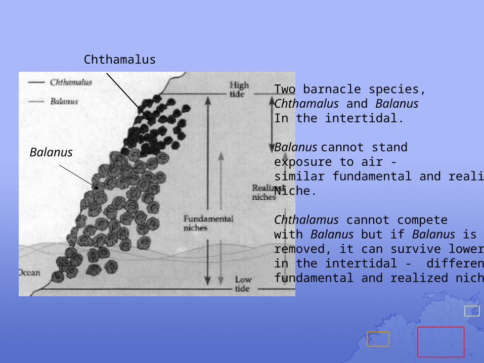
HOW CAN WE RECONSTRUCT THE FUNDAMENTAL NICHE?(we can start by looking at where a species occurs)
Poecile gambeli – Mountain chickadee
Dots are occurrences of Poecile gambeli across its range
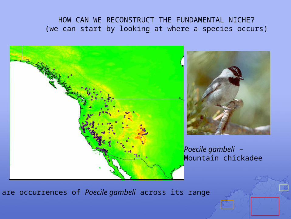
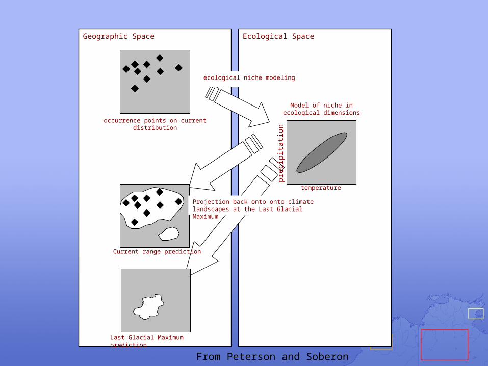
How Can We Model the Fundamental Niche?
Geographic Space Ecological Space
occurrence points on current distribution
ecological niche modeling
temperature
Model of niche in ecological dimensions
prec
ipita
tion
Geographic Space Ecological Space
occurrence points on current distribution
ecological niche modeling
Projection back onto onto climate landscapes at the Last Glacial Maximum
Current range prediction
Last Glacial Maximum prediction
temperature
Model of niche in ecological dimensions
prec
ipita
tion
From Peterson and Soberon

SOME TERMINOLOGY
Geographic Space Environmental Space
G is the geographic space, typically composed of 2-D pixels
Ga , Gp = The abiotically suitable area(potential distribution)
Gb = The biotically suitable area
Gm = Accessable area through dispersal
Gi = Invadable distributional area
Go = Occupied distributional area
Gdata = set of observations (presences, and, if existing, true absences).
E Environmental space of environmentalvariables.
Ea Scenopoetic fundamental niche
Ei Invadable niche space
Eo Occupied niche space
Ep Biotically reduced niche

Example Mapping Between Geographic Space and Environmental Space
Go is shown as gray shading, and Ga is “white”
EaEo
Note:This Area is occupiedbut not sampled --- (because you areOmiscientIn this example.Work with me.)
Porque no occupado?
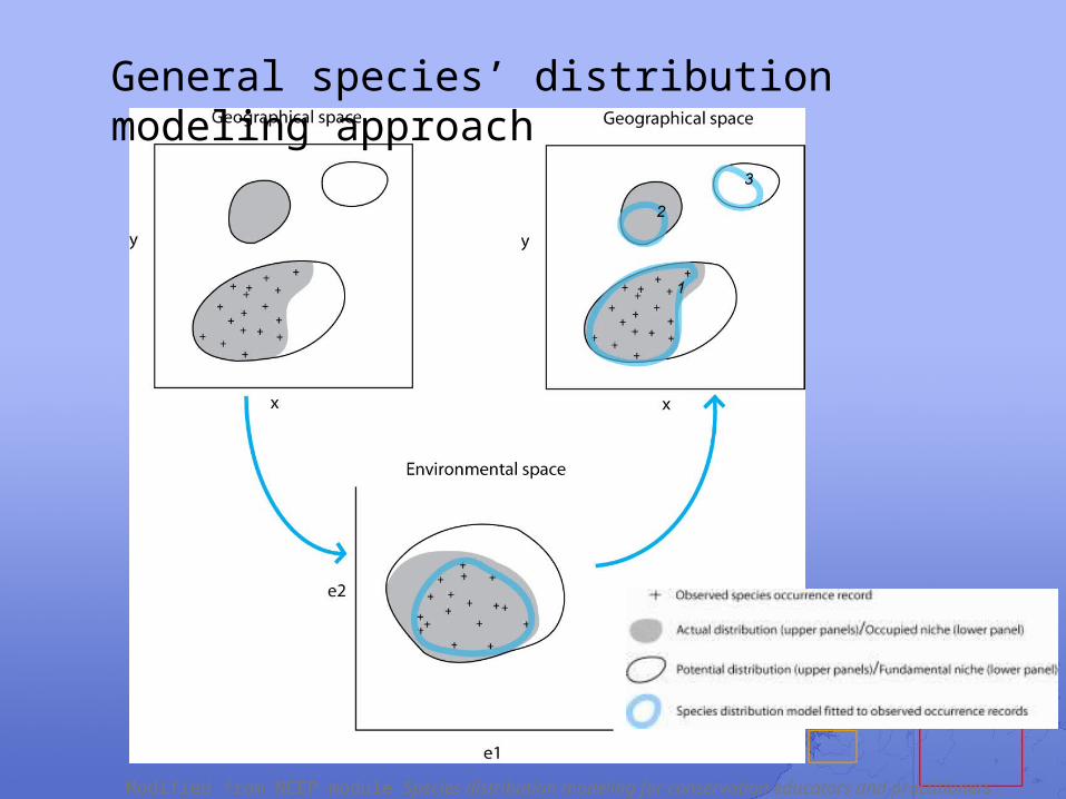
General species’ distribution modeling approach
Modified from NCEP module Species distribution modeling for conservation educators and practitioners.
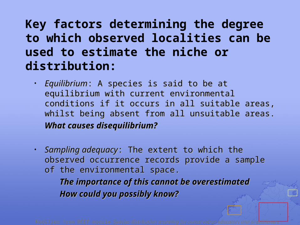
Key factors determining the degree to which observed localities can be used to estimate the niche or distribution:
• EquilibriumEquilibrium: A species is said to be at equilibrium : A species is said to be at equilibrium with current environmental conditions if it occurs in with current environmental conditions if it occurs in all suitable areas, whilst being absent from all all suitable areas, whilst being absent from all unsuitable areas. unsuitable areas.
What causes disequilibrium? What causes disequilibrium?
• Sampling adequacySampling adequacy: The extent to which the : The extent to which the observed occurrence records provide a sample of the observed occurrence records provide a sample of the environmental space.environmental space.
The importance of this cannot be The importance of this cannot be overestimatedoverestimated
How could you possibly know?How could you possibly know?
Modified from NCEP module Species distribution modeling for conservation educators and practitioners.
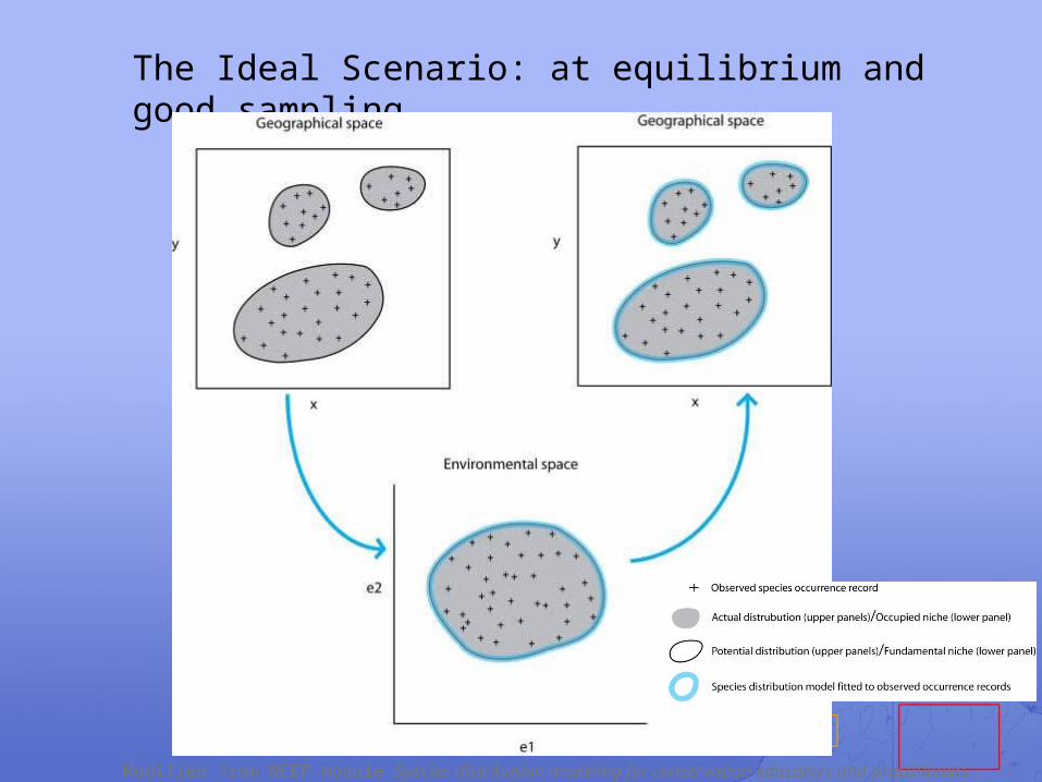
The Ideal Scenario: at equilibrium and good sampling
Modified from NCEP module Species distribution modeling for conservation educators and practitioners.
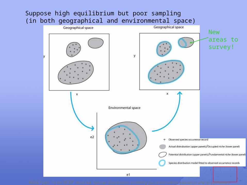
Suppose high equilibrium but poor sampling (in both geographical and environmental space)
Modified from NCEP module Species distribution modeling for conservation educators and practitioners.
New areas to survey!

Suppose high equilibrium and poor sampling in geographical space,but good sampling in environmental space
Modified from NCEP module Species distribution modeling for conservation educators and practitioners.

Suppose low equilibrium but good sampling
Modified from NCEP module Species distribution modeling for conservation educators and practitioners.
Potential Distribution
Fundamental Niche


• Circle A represents area where abiotic conditions are right for a species to occur (Ga)
• Circle B represent the area where lack of competition, disease, and occurrence of mutualists allows populations to grow.
• Circle M is area within which individuals & populations are capable of moving due to lack of dispersal barriers.
• Go is occupied area
• Gi is invadable area
Note: niche modeling pulls occurrences from that intersection.
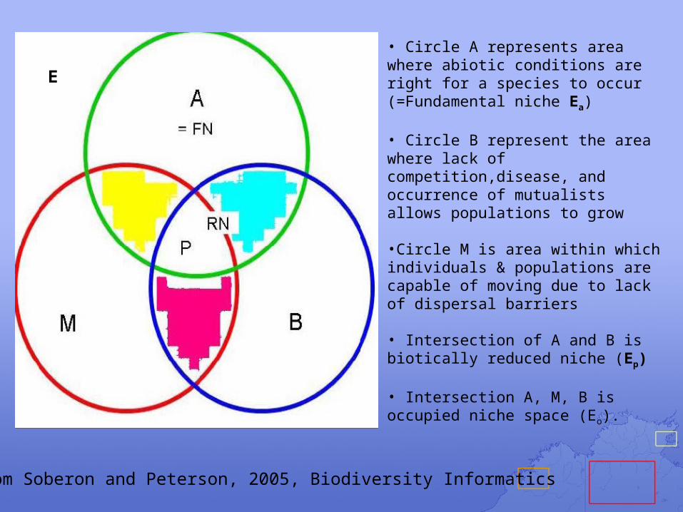
• Circle A represents area where abiotic conditions are right for a species to occur (=Fundamental niche Ea)
• Circle B represent the area where lack of competition,disease, and occurrence of mutualists allows populations to grow
•Circle M is area within which individuals & populations are capable of moving due to lack of dispersal barriers
• Intersection of A and B is biotically reduced niche (Ep)
• Intersection A, M, B is occupied niche space (Eo).
E
From Soberon and Peterson, 2005, Biodiversity Informatics

Best Case: Weak, diffuseabiotic interactions andlack of dispersal barrierscreate general overlap.
No dispersal barriers, butarea of “correct” bioticinteractions different fromarea of correct abiotic conditions. Estimate of FNusing occurrence data shouldbe carefully examined
FN (and potential distribution)will be much largerthan actual distribution due to dispersal limitations
SOME POSSIBLE OUTCOMES
From Soberon and Peterson, 2005, Biodiversity Informatics
What abiotic factors determine fundamental niche?
• The answer is complicated (but important)• Species have physiological tolerances, migration
limitations and evolutionary forces that limit adaptation
• A starting point for physiology may be traits• A starting point for abiotic factors is often climate• Climate variables often also correlate with other
variables (elevation, land cover)
“Easy” In Theory --- But how does it work in practice?
• The development of spatial ecological modeling approaches occurs in 90s
• But has origins in ongoing innovations from the 70s forward
• A bit of history…
How do we in practice model the “scenopoetic” ecological niche?
and
How do we determine a species distribution (actual and potential)
and what is the difference?
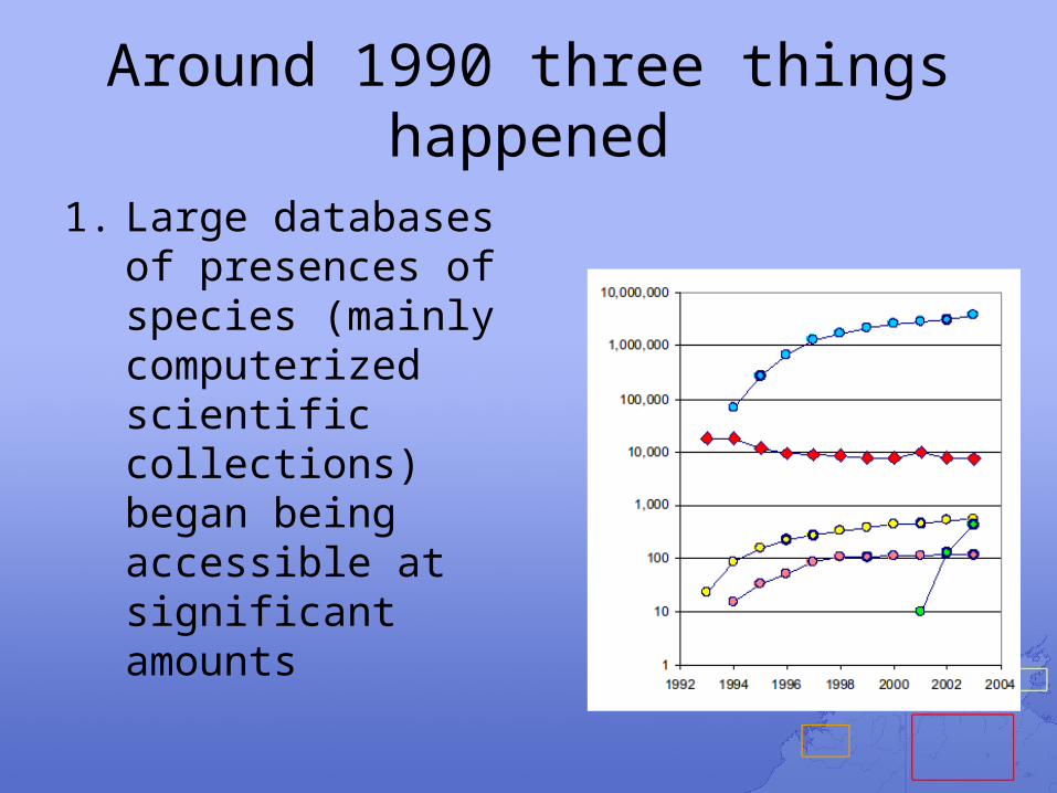
Around 1990 three things happened
1. Large databases of presences of species (mainly computerized scientific collections) began being accessible at significant amounts
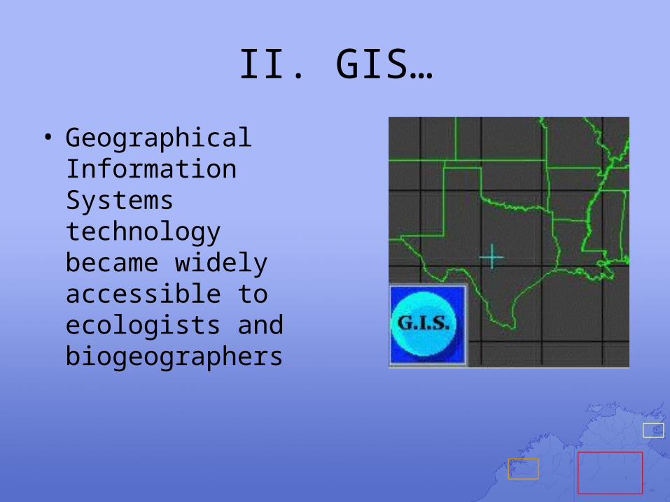
II. GIS…
• Geographical Information Systems technology became widely accessible to ecologists and biogeographers

IV. Worldwide Environmental Data Layers
• Remote sensing data – Land cover/land type– Vegetation– Terrain– Ocean SST, chlorophyll
• Slope, aspect, flow rate hydrology data• Climatology databases
– Worldclim (what we’ll use in this class)– Models of worldwide past and future climates (IPCC)
• All other ancillary data layers (roads, human population density, etc)

Which leads to an NCEAS Working Group
Title: Choosing (and making available) the right environmental layers for modeling how the environment controls the distribution and abundance of organisms
Aim: To generate co-registered environmental data layers at 1km resolution representing climate, vegetation/landcover, hydrology/topography, marine.

A TOUGH GIG (Actually this meeting was a lot of work!)
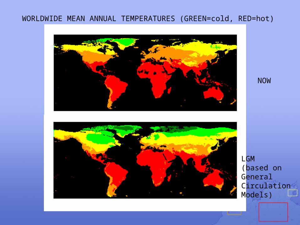
WORLDWIDE MEAN ANNUAL TEMPERATURES (GREEN=cold, RED=hot)
NOW
LGM (based onGeneralCirculationModels)
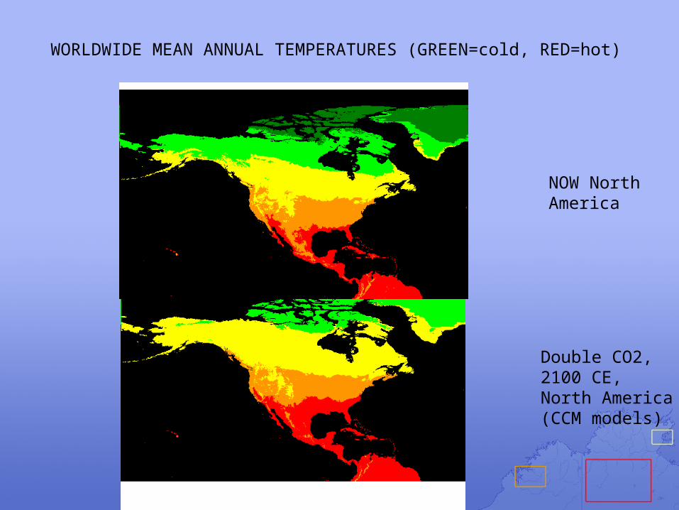
WORLDWIDE MEAN ANNUAL TEMPERATURES (GREEN=cold, RED=hot)
NOW NorthAmerica
Double CO2,2100 CE, North America(CCM models)

temperature
precipitation
elevation
soils
Inputs into a nichemodel:
•stack of environmental data layers
•Set of occurrence records representing presences
Occurrence record

NICHE AND DISTRIBUTION MODELING
Input: Species Presence
Input Env. Data Layers
CAN WE PREDICT NICHE AND DISTRIBUTIONFROM SUCH DATA? (answer: maybe!)
From Maxent presentation by Pearson
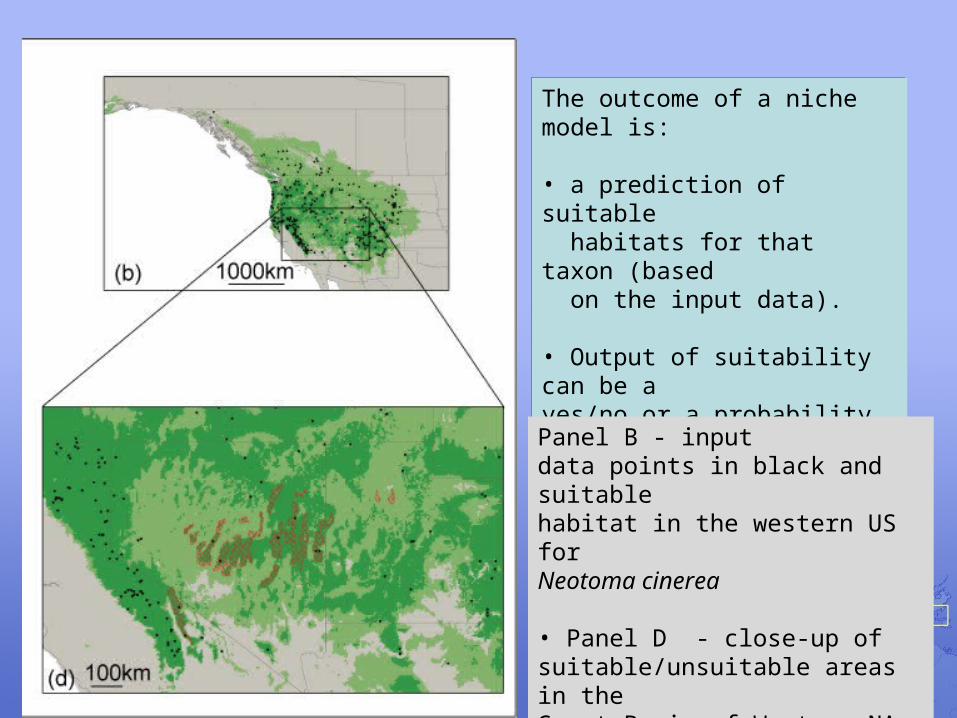
The outcome of a niche model is:
• a prediction of suitable habitats for that taxon (based on the input data).
• Output of suitability can be a yes/no or a probability functionfrom 0-100.
The outcome of a niche model is:
• a prediction of suitable habitats for that taxon (based on the input data).
• Output of suitability can be a yes/no or a probability functionfrom 0-100.
Panel B - input data points in black and suitablehabitat in the western US forNeotoma cinerea
• Panel D - close-up of suitable/unsuitable areas in theGreat Basin of Western NA.
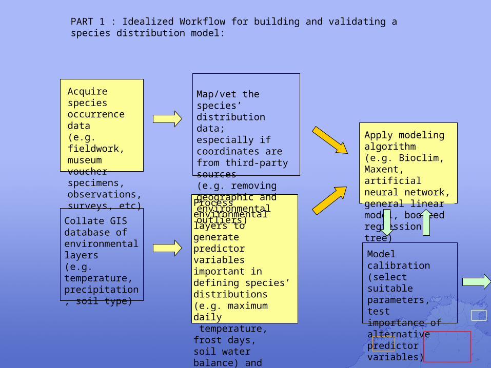
PART 1 : Idealized Workflow for building and validating a species distribution model:
Process environmental layers to generate predictor variables important in defining species’ distributions (e.g. maximum daily temperature, frost days, soil water balance) and convert to appropriate formats
Map/vet the species’ distribution data;especially if coordinates are from third-party sources (e.g. removing geographic and environmental outliers)
Collate GIS database of environmental layers (e.g. temperature, precipitation, soil type)
Apply modeling algorithm(e.g. Bioclim, Maxent, artificial neural network, general linear model, boosted regression tree)
Model calibration(select suitable parameters, test importance of alternative predictor variables)
Acquire species occurrence data(e.g. fieldwork, museum voucher specimens, observations, surveys, etc)

Create map of current modeled distribution
Model species’ distribution in a different region (e.g. for an invasive species) or for a different time period (e.g. under future climate scenario)
Test model performance through additional fieldwork or statistical approach (e.g. AUC or Kappa or null model comparisons)
If possible, test model against observed data, such as occurrence records in an invaded region, or distribution shifts over recent decades
PART 2 : Idealized Workflow for building and validating a species distribution model:
Modified from NCEP module Species distribution modeling for conservation educators and practitioners.

A stopping point
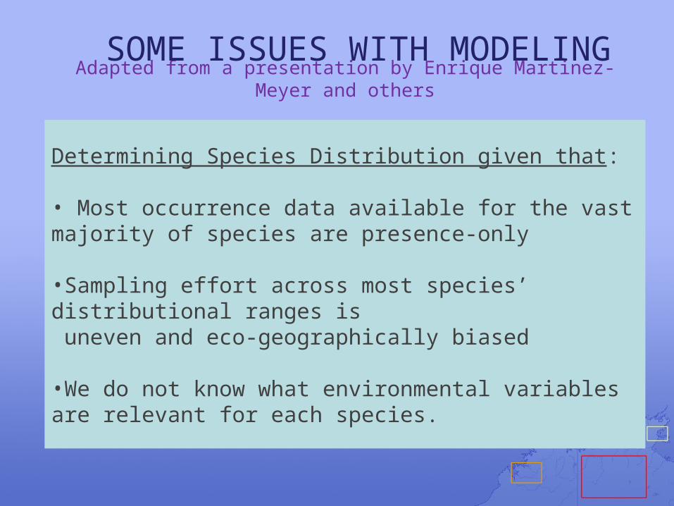
Determining Species Distribution given that:
• Most occurrence data available for the vast majority of species are presence-only
•Sampling effort across most species’ distributional ranges is uneven and eco-geographically biased
•We do not know what environmental variables are relevant for each species.
Adapted from a presentation by Enrique Martinez-Meyer and others
SOME ISSUES WITH MODELING
Modeling Niches
• All niche modeling approaches model the function approximating the true relationship between the environment (i.e., the niche) and species geographic occurrences/distribution.
Modeling Niches P2
• All want to estimate function f = μ(Gdata, E) - that is the result of applying an algorithm to data given an environmental space E to estimate G (distribution)
• Different algorithms have different data requirements– True presence-only– Presence-absence– Presence-background (can be any sample from within
environment)– Presence-pseudoabsence (a pseudoabsence cannot be where a
species is known to occur)

Algorithms Applied to the ProblemMethod(s) Model/software name Species data type
Climatic envelope BIOCLIM Presence-only
Gower Metric DOMAIN Presence-only
Ecological Niche Factor Analysis (ENFA) BIOMAPPER Presence/background
Maximum Entropy MAXENT Presence/background
Genetic algorithm GARP Presence/pseudo-absence
Regression: Generalized linear model (GLM) and Generalized additive model (GAM)
GRASP Presence/absence
Artificial Neural Network (ANN) SPECIES Presence/absence
Classification and regression trees (CART), GLM, GAM and ANN
BIOMOD Presence/absence
Boosted decision trees (implemented in R) Presence/absence
Multivariate adaptive regression splines (MARS)
(implemented in R) Presence/absence
From Richard Pearson et al. 2006
Niche Modeling Has Problems PT 2Niche Modeling Has Problems PT 2tradeoffs w/algorithmstradeoffs w/algorithms
- Many algorithms do not handle asymmetric data (e.g. GLM, GAM)
-Many don’t handle interaction effects (BioClim)
- Some of the do not handle nominal environmental variables (e.g. soil classes) [e.g. BioClim, ENFA]
- Many stochastic algorithms present different solutions even under identical parameterization and input data (e.g. GARP)
- We do not know the ‘real’ distribution of species, so we do not know when models are making mistakes and when are filling knowledge gaps.
Modeling Approaches• Presence only (bioclimatic envelopes or mahalanobis distance) – points
inside envelope suitable or distance of points away from mean values (farther away equals less suitable)
• Presence-absence – GAMs, GLMs, MARs, CARTs. Use a link or function or set of logical statements describing the multivariate relationship between mean of response variable and predictor variables. Note: best for determining occupied distribution (not potential dist.)
• Presence-background – Maxent finds the probability distribution most spread out, or closest to uniform, subject to constraints given observed occurrence records information and environmental conditions across study area. All regression techniques work with background as well.
• Presence-pseudoabsence – GARP. Rule set predictions.

Example of Presence-Only Envelope Approach - BioClim
• Heuristic based model• Works with presence-only data • Simple to use• 35-dimensional Hypercube in climate-
space (19 in Diva-GIS)• Tends to over-predict• Works with small number of records• Will work in batch mode• Can’t make quantitative predictions or
provide confidence levels• Used for predicting potential
distributions• Versions incorporated into Diva-GIS

BioClim Type Modeling
•The dot-dash line square is the BioClim fit of the data (for two dimensions )
•This defines an range of the values in the occupied by a species across all environmental variables for all axes.
•Anything in this box might be considered “suitable”.
From Peterson et al. ms. Ecological Niches and Geographic Distributions:A Modeling Perspective

Presence-Background Modeling
• No known absences• How to determine false absences from true absences
then?• Solution (of sorts): Compare background is the set of
grid cells used in modeling• Note: These points include input true presences
Question: What does this mean for model validation?
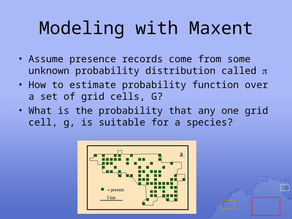
Modeling with Maxent
• Assume presence records come from some unknown probability distribution called
• How to estimate probability function over a set of grid cells, G?
• What is the probability that any one grid cell, g, is suitable for a species?
Modeling in Maxent
annual minimum coolest month
maximum warmest month
range coolestquarter
warmestquarter
Wettestquarter
dryestquarter
Mean 17.2 6.2 26.1 19.9 12.3 21.3 20.0 13.8
S.D. 1.8 2.0 1.6 2.0 2.1 1.6 3.6 2.0
Min 12.1 0.2 23.9 18.1 5.8 18.3 5.8 10.6
5%-ile 12.1 0.2 23.9 18.1 5.8 18.3 5.8 10.6
25%-ile 16.4 6.1 24.6 18.5 11.8 20.2 19.9 2.5
75%-ile 18.3 6.1 7.2 20.2 12.8 2.8 21.3 14.8
95%-ile 19.6 9.2 29.0 23.0 15.2 23.7 23.4 17.6
max 19.6 9.2 29.4 25.4 15.2 23.8 23.6 17.6
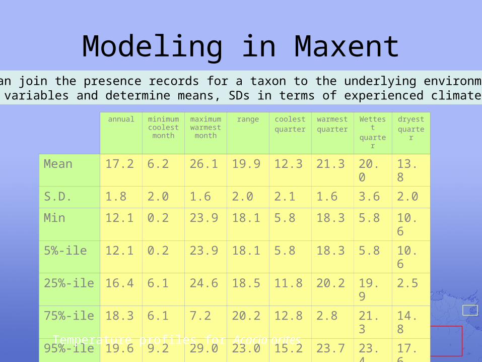
We can join the presence records for a taxon to the underlying environmentalvariables and determine means, SDs in terms of experienced climate
Temperature profiles for Acacia orites

Modeling with Maxent
• Each grid cell has a set of “features” defined by the environment.
• Features can be the raw environment or some more complex function of those environmental variables (linear, quadratic, logistic)
• Grid cells with presences can be summed to determine means and SDs across all environmental variables in order to estimate
• Means of the probability distribution match the observed means
• Find the flattest function (one that maximizes entropy)
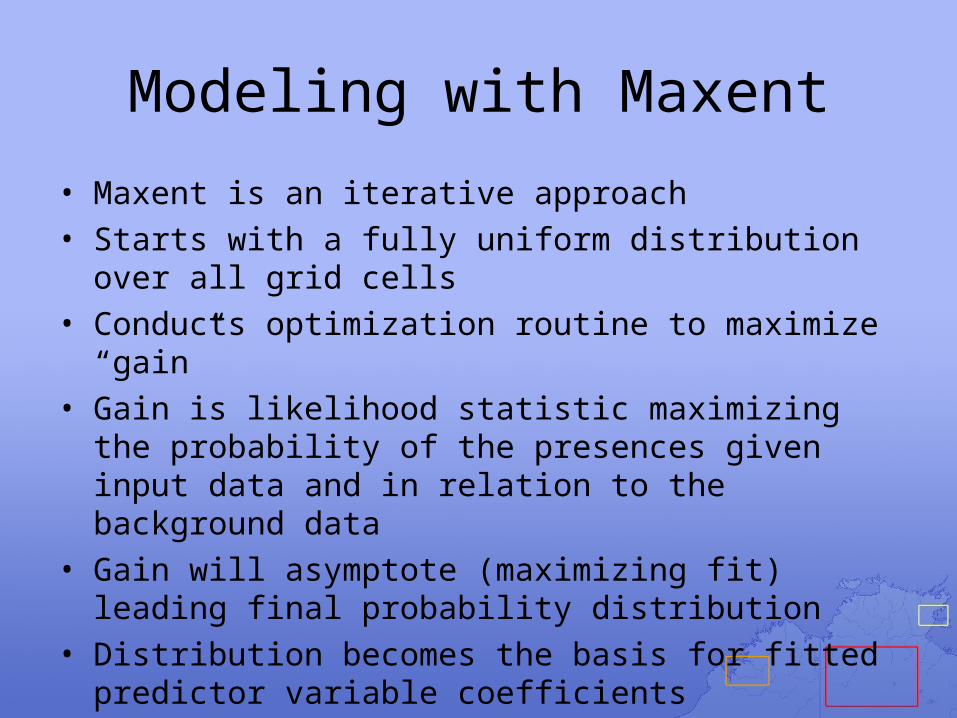
Modeling with Maxent
• Maxent is an iterative approach• Starts with a fully uniform distribution over all grid cells• Conducts optimization routine to maximize “gain”• Gain is likelihood statistic maximizing the probability of
the presences given input data and in relation to the background data
• Gain will asymptote (maximizing fit) leading final probability distribution
• Distribution becomes the basis for fitted predictor variable coefficients
• These coefficients are used to assess probability of presence

Maxent
• Maxent is run by first selecting a set of input environmental data layers in a common GIS forrmat (gridded .ASC giles)
• Next select a set of species occcurrence locations defined by lat/lon
• Important to subset data into training and testing. Training data builds model, testing data is used for validation

More on Maxent
• maximum spread = maximizing the log likelihood of the data associated with the presence sites minus a penalty term (think AIC)
• Penalty term is basically related to a weighting based on how much information the environmental data adds to the model.
• The best weighting term is discovered through a sequential updating algorithm run a specified number of iterations (you can change this parameter)

More on Maxent
• Maxent regularization parameter determines “penalty function” - smaller values tend to overfit models (typically leading to smaller geo. distributions) & larger values do the opposite.
• You can choose culmulative versus logistic outputs. Logistic is interpreted as probability of presence (e.g. what you most often want)
• Definitely create response curves
• What about features?
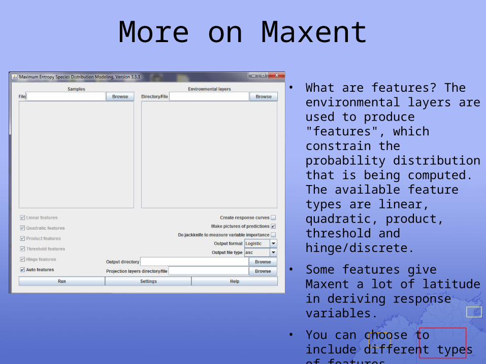
More on Maxent
• What are features? The environmental layers are used to produce "features", which constrain the probability distribution that is being computed. The available feature types are linear, quadratic, product, threshold and hinge/discrete.
• Some features give Maxent a lot of latitude in deriving response variables.
• You can choose to include different types of features

More on Maxent
What does a Maxent run produce?
•A HTML file showing run outputs•A grid file importable into a GIS•CSV files containing ommission, •prediction details
Focus on the HTML file, which contains:
• A picture of the map• A table of different thresholds *• A model validation statistical summary *• An explanation of importance of variables• Response curves
* we’ll discuss model validation tomorrow