Introduction to Partial Identification - Paul Scottptscott.com/teaching/tse_eio_2014/partial-identification-overview.pdf · Introduction First insights Inference in model with partial

Introduction to Partial Identification

C. Bontemps1

1Toulouse School of Economics

DEEQA - Winter 2014

IntroductionFirst insights

Inference in model with partial identificationThe criterion approach

The convex approachConclusion

A first example

Partial Identification in Econometrics I

The traditional approach in statistics and econometrics is to considermodels that are point identified.Given an infinite amount of data, in such models one can alwaysinfer without uncertainty what the values of the objects of interestare.Uncertainty about the true value of a parameter is thus only due tousing a finite data set.Researchers traditionally felt uncomfortable about models in whichpoint identification fails.They have therefore often added additional assumptions to theirmodels that have identifying power, even if they are not well justifiedby economic theory.Problem: Empirical results might be driven by a priori assumptions,and not by the data.

Two researchers using the same data set might come to differentconclusions, depending on which additional assumptions they impose.

C. Bontemps Introduction to Partial Identification




A first example

Partial Identification in Econometrics II

It is therefore important to find out what conclusions can be drawnabout a research question under weaker or minimal assumptions.This sometimes means that one has to give up point identification.That is, one has to work with a model where it is not possible toinfer the true value of the parameter of interest even with aninfinitely large data set.Such models are not useless!The data might reveal some non-trivial insights about the objects ofinterest, even though they do not allow for an exact quantification.This perspective is called partial identification.

Partial identification occurs in many areas of applied econometrics:measurement error model,missing data models,treatment effects,market entry games,Economic models with inequalities.





A first example

Partial Identification in Econometrics III

Partial identification analysis is about finding out which values of thetrue parameter of interest are compatible with the observations wemade.

How can we obtain the identified set?Partial identification also poses new challenges for estimation andinference:

How can we obtain “estimates” in a setting where consistentestimation is impossible?How can we test an hypothesis about the parameter of interest?





A first example

Linear Error-in-Variables Models I

Frisch (1934) studied linear regression problems when variables aremeasured with error.Suppose that there is a linear model

Y ∗ = β1 +β2X∗+ε

where Y ∗,X∗,ε are scalar and E [ε] = 0, E [X∗ε] = 0.Assume that both Y ∗ and X∗ are observed with error:

Y = Y ∗+ ∆YX = X∗+ ∆X

Here ∆Y and ∆X are unobserved measurement errors that areuncorrelated with the other primitives of the model.Question: What can we learn from observing (Y ,X ) about theslope parameter β2 in the true regression?





A first example

Linear Error-in-Variables Models II

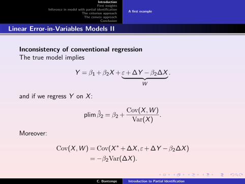
Inconsistency of conventional regressionThe true model implies

Y = β1 +β2X +ε+ ∆Y −β2∆X︸︷︷︸W

.

and if we regress Y on X :

plim β2 = β2 +Cov(X ,W )

Var(X ).

Moreover:

Cov(X ,W ) = Cov(X∗+ ∆X ,ε+ ∆Y −β2∆X )

=−β2Var(∆X ).





A first example

Linear Error-in-Variables Models III

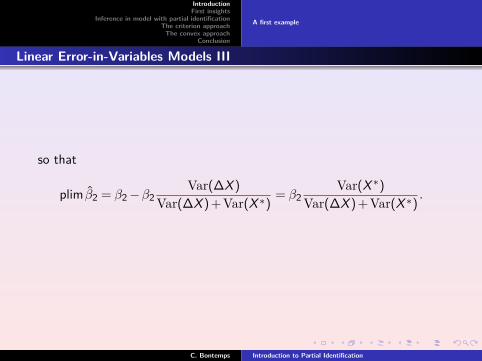
so that

plim β2 = β2−β2Var(∆X )

Var(∆X ) + Var(X∗) = β2Var(X∗)

Var(∆X ) + Var(X∗) .





A first example

Linear Error-in-Variables Models IV

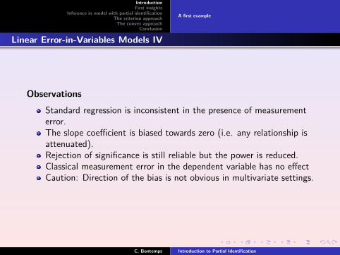
Observations

Standard regression is inconsistent in the presence of measurementerror.The slope coefficient is biased towards zero (i.e. any relationship isattenuated).Rejection of significance is still reliable but the power is reduced.Classical measurement error in the dependent variable has no effectCaution: Direction of the bias is not obvious in multivariate settings.





A first example

Linear Error-in-Variables Models V

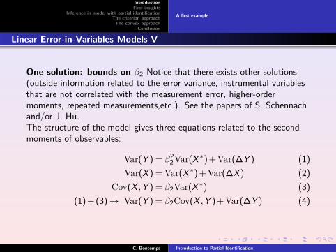
One solution: bounds on β2 Notice that there exists other solutions(outside information related to the error variance, instrumental variablesthat are not correlated with the measurement error, higher-ordermoments, repeated measurements,etc.). See the papers of S. Schennachand/or J. Hu.The structure of the model gives three equations related to the secondmoments of observables:

Var(Y ) = β22Var(X∗) + Var(∆Y ) (1)

Var(X ) = Var(X∗) + Var(∆X ) (2)Cov(X ,Y ) = β2Var(X∗) (3)

(1) + (3)→ Var(Y ) = β2Cov(X ,Y ) + Var(∆Y ) (4)





A first example

Linear Error-in-Variables Models VI

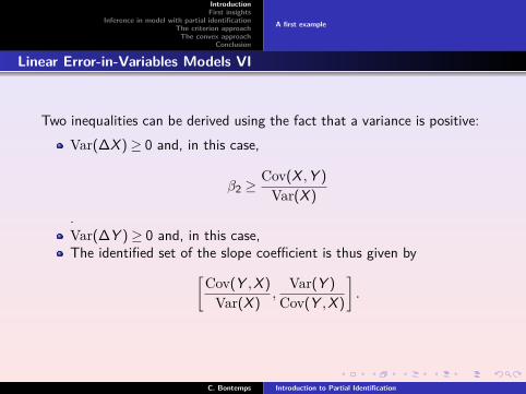
Two inequalities can be derived using the fact that a variance is positive:Var(∆X )≥ 0 and, in this case,

β2 ≥Cov(X ,Y )

Var(X )

.Var(∆Y )≥ 0 and, in this case,The identified set of the slope coefficient is thus given by[

Cov(Y ,X )

Var(X ),

Var(Y )

Cov(Y ,X )

].





A first example

Linear Error-in-Variables Models VII

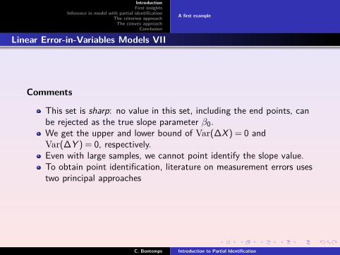
Comments

This set is sharp: no value in this set, including the end points, canbe rejected as the true slope parameter β0.We get the upper and lower bound of Var(∆X ) = 0 andVar(∆Y ) = 0, respectively.Even with large samples, we cannot point identify the slope value.To obtain point identification, literature on measurement errors usestwo principal approaches





A first example

Road Map

1 Some (usual) examples of interest2 The Moment inequality approach

The original paperAndrews and co.further discussion

3 Convexity and the support function approach4 Conclusion and perspective





DefinitionSome Examples

A more formal definition I

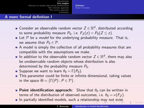
Consider an observable random vector Z ∈ Rd , distributed accordingto some probability measure P0, i.e. FZ (z) = P0(Z ≤ z).Let P be a model for the underlying probability measure. That is,we assume that P0 ∈ P.A model is simply the collection of all probability measures that arecompatible with the assumptions we make.In addition to the observable random vector Z ∈ Rd , there may alsobe unobservable random objects whose distribution is alsodetermined by the probability measure P0.Suppose we want to learn θ0 = Γ(P0).This parameter could be finite or infinite dimensional, taking valuesin the space Θ = Γ(P) : P ∈ P.

Point identification approach: Show that θ0 can be written interms of the distribution of observed outcomes, i.e. θ0 = ν(FZ ).In partially identified models, such a relationship may not exist.






A more formal definition II

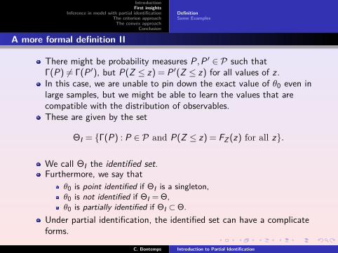
There might be probability measures P,P ′ ∈ P such thatΓ(P) 6= Γ(P ′), but P(Z ≤ z) = P ′(Z ≤ z) for all values of z .In this case, we are unable to pin down the exact value of θ0 even inlarge samples, but we might be able to learn the values that arecompatible with the distribution of observables.These are given by the set

ΘI = Γ(P) : P ∈ P and P(Z ≤ z) = FZ (z) for all z.

We call ΘI the identified set.Furthermore, we say that

θ0 is point identified if ΘI is a singleton,θ0 is not identified if ΘI = Θ,θ0 is partially identified if ΘI ⊂Θ.

Under partial identification, the identified set can have a complicateforms.






A more formal definition III

One of the most important challenges when working with partiallyidentified models is to find a simple characterization for theidentified set.






Examples

Partial identification issues were studied as early as in the 1930’s(and probably earlier).This research had little impact on applied economics.

Recent interest in partial identification started with the work ofManski in the 1990’s.

We now consider two of the leading examples considered in thisliterature. Additional examples are

Bounds on the Joint CDF with given MarginalsMissing Data and Treatment EffectsLinear Models with Interval censored regressors






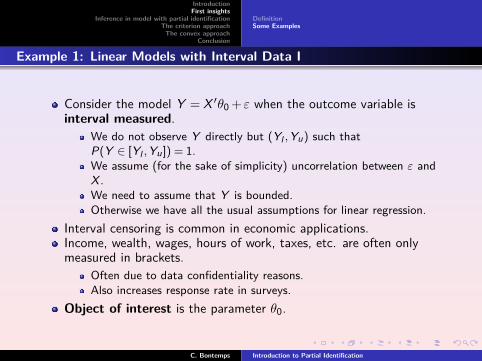
Example 1: Linear Models with Interval Data I

Consider the model Y = X ′θ0 +ε when the outcome variable isinterval measured.

We do not observe Y directly but (Yl ,Yu) such thatP(Y ∈ [Yl ,Yu]) = 1.We assume (for the sake of simplicity) uncorrelation between ε andX .We need to assume that Y is bounded.Otherwise we have all the usual assumptions for linear regression.

Interval censoring is common in economic applications.Income, wealth, wages, hours of work, taxes, etc. are often onlymeasured in brackets.

Often due to data confidentiality reasons.Also increases response rate in surveys.

Object of interest is the parameter θ0.






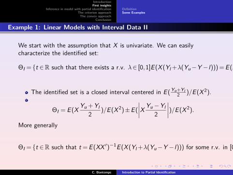
Example 1: Linear Models with Interval Data II

We start with the assumption that X is univariate. We can easilycharacterize the identified set:

ΘI = t ∈R such that there exists a r.v. λ∈ [0,1]E (X (Yl +λ(Yu−Y − l))) = E (X 2)t

The identified set is a closed interval centered in E ( Yu+Yl2 )/E (X 2).

ΘI = E (X Yu + Yl2 )/E (X 2)±E (

∣∣∣∣X Yu−Yl2

∣∣∣∣)/E (X 2).

More generally

ΘI = t ∈R such that t = E (XX ′)−1E (X (Yl +λ(Yu−Y − l))) for some r.v. in [0,1]






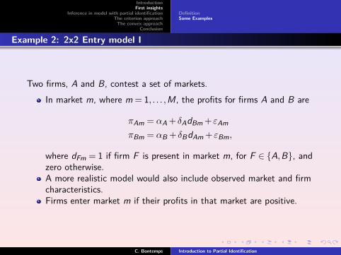
Example 2: 2x2 Entry model I

Two firms, A and B, contest a set of markets.In market m, where m = 1, . . . ,M, the profits for firms A and B are

πAm = αA + δAdBm +εAm

πBm = αB + δBdAm +εBm,

where dFm = 1 if firm F is present in market m, for F ∈ A,B, andzero otherwise.A more realistic model would also include observed market and firmcharacteristics.Firms enter market m if their profits in that market are positive.






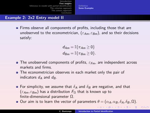
Example 2: 2x2 Entry model II

Firms observe all components of profits, including those that areunobserved to the econometrician, (εAm,εBm), and so their decisionssatisfy:

dAm = IπAm ≥ 0dBm = IπBm ≥ 0.

The unobserved components of profits, εFm, are independent acrossmarkets and firms.The econometrician observes in each market only the pair ofindicators dA and dB .

For simplicity, we assume that δA and δB are negative, and that(εAm,εBm) has a distribution FΩ that is known up tofinite-dimensional parameter Ω.Our aim is to learn the vector of parameters θ = (αA,αB , δA, δB ,Ω).






Example 2: 2x2 Entry model III

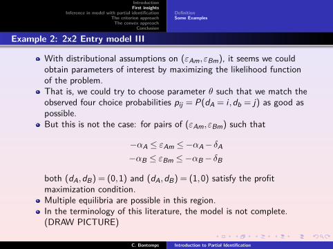
With distributional assumptions on (εAm,εBm), it seems we couldobtain parameters of interest by maximizing the likelihood functionof the problem.That is, we could try to choose parameter θ such that we match theobserved four choice probabilities pij = P(dA = i ,db = j) as good aspossible.But this is not the case: for pairs of (εAm,εBm) such that

−αA ≤ εAm ≤−αA− δA

−αB ≤ εBm ≤−αB− δB

both (dA,dB) = (0,1) and (dA,dB) = (1,0) satisfy the profitmaximization condition.Multiple equilibria are possible in this region.In the terminology of this literature, the model is not complete.(DRAW PICTURE)






Example 2: 2x2 Entry model IV

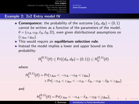
Consequence: the probability of the outcome (dA,dB) = (0,1)cannot be written as a function of the parameters of the model,θ = (αA,αB , δA, δB ,Ω), even given distributional assumptions on(εAm,εBm).This would require an equilibrium selection rule.Instead the model implies a lower and upper bound on thisprobability:

H(0,1)L (θ)≤ Pr((dA,dB) = (0,1))≤ H(0,1)

U (θ)

where

H(0,1)L (θ) = Pr(εAm <−αA,−αB < εBm)

+ Pr(−αA < εAm <−αA− δA,−αB− δB < εBm)

and

H(0,1)U (θ) = Pr(εAm <−αA− δA,−αB < εBm).






Example 2: 2x2 Entry model V

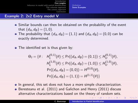
Similar bounds can then be obtained on the probability of the eventthat (dA,dB) = (1,0).The probability that (dA,dB) = (1,1) and (dA,dB) = (0,0) can beexactly determined.

The identified set is thus given by:

ΘI = θ : H(0,1)L (θ)≤ Pr((dA,dB) = (0,1))≤ H(0,1)

U (θ),

H(1,0)L (θ)≤ Pr((dA,dB) = (1,0))≤ H(1,0)

U (θ),

Pr((dA,dB) = (0,0)) = H(0,0)(θ),

Pr((dA,dB) = (1,1)) = H(1,1)(θ)

In general, this set does not have a more simple characterization.Beresteanu et al. (2011) and Galichon and Henry (2011) discussalternative characterizations based on the theory of random sets.






Example 2: 2x2 Entry model VI

Tamer (2003) shows that if profits are of the form

πFm = αF + X ′FmβF + δF dFm +εFm, F ∈ A,B,

where XF are observable firm characteristics, one can achieve pointidentification under a large support condition on one of thecharacteristics (“identification at infinity”).





General commentsInference in an interval identified model

General comments I

Partial identification creates new and interesting issues forestimation and inference.

How do we estimate a set?What is a “good” estimate of a set?How do we construct a confidence region for a set?Can we test an hypothesis about the true parameter under partialidentification?

For more complicated models where the identified set is difficult todescribe explicitly, such questions are still the object of currentresearch.We also discuss the difference between covering a set or any point ofthe setUniformity of the approach with respect to the (true but unknown)size of the set.






General comments II

One can try to obtain an estimate ΘI of the identified set ΘI .Depending on the shape of the identified set, one can use differentapproaches to obtain such an estimate (we talk about this soon).Question: Which theoretical properties should such an estimator ΘIhave, independently of the method used to construct it?This issue needs clarification, as most standard notions from pointestimation have no immediate counterpart for set estimation.






General comments III

At a minimum, such an estimator should be consistent.What does this mean?As the sample size increases, ΘI should get closer to ΘI :

d(ΘI ,ΘI)p→ 0

for some distance measure d(·, ·) that works for sets.The literature on partial identification has most commonly used theHausdorff distance:

dH(A,B) = maxsupa∈A

infb∈B‖a−b‖, inf

a∈Asupb∈B‖a−b‖.

Other distance measures are possible in principle, but are rarelyconsidered.Other common properties of point estimators, like asymptoticnormality or efficiency are difficult to transfer to set estimation.






Estimation: Interval Identified Parameters I

Estimation is straightforward if the true parameter θ0 is scalar andthe identified set takes the form of an interval, i.e.

ΘI = [θl ,θu].

In this case, we can estimate ΘI by

ΘI = [θl , θu],

where θl , θu are suitable estimates of the upper and lower boundaryof the interval.It is straightforward to show that if (θl , θu)

p→ (θl ,θu) the setestimator ΘI is consistent in the Hausdorff norm.Proof: dH(ΘI ,ΘI) = max‖θl −θl‖,‖θu−θu‖

p→ 0






Estimation: Interval Identified Parameters II

Example (Interval censoring with one explanatory variable):Observe (Yui ,Yli ,Xi ), where Yi ∈ [Yli ,Yui ] is the outcome of interest.Recall that the identified set is

ΘI =E ( X(Yu+Yl )

2 )

E (X 2)±

E (∣∣∣X Yu−Yl

2

∣∣∣)E (X 2)

.

Estimation by sample analogues: put

θc =1n∑n

i=1 Xi (Yui + Yli )

2 1n∑n

i=1 X 2i

and hl =1n∑n

i=1 |Xi |(Yui −Yli )

2 1n∑n

i=1 X 2i

and set

θl = θc − hl and θu = θc + hl .

Consistency follows from Law of Large Numbers and ContinuousMapping Theorem.






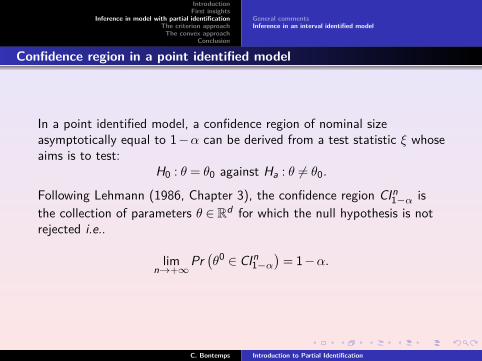
Confidence region in a point identified model

In a point identified model, a confidence region of nominal sizeasymptotically equal to 1−α can be derived from a test statistic ξ whoseaims is to test:

H0 : θ = θ0 against Ha : θ 6= θ0.

Following Lehmann (1986, Chapter 3), the confidence region CIn1−α is

the collection of parameters θ ∈ Rd for which the null hypothesis is notrejected i.e..

limn→+∞

Pr(θ0 ∈ CIn

1−α)

= 1−α.






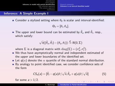
Inference: A Simple Example I

Consider a stylized setting where θ0 is scalar and interval-identified:

ΘI = [θl ,θu].

The upper and lower bound can be estimated by θu and θl , resp.,which satisfy:

√n((θu, θl )− (θu,θl ))

d→ N(0,Σ)

where Σ is a diagonal matrix with diag(Σ) = (σ2u,σ

2l ).

We thus have asymptotically normal and independent estimated ofthe upper and lower boundaries of the identified set.Let q(α) denote the α quantile of the standard normal distribution.By analogy to point identified case, we consider confidence sets ofthe form

CSn(a) = [θl −q(a)σ/√

n, θu + q(a)σ/√

n] (5)

for some a > 1/2.C. Bontemps Introduction to Partial Identification





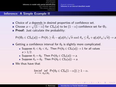
Inference: A Simple Example II

Choice of a depends in desired properties of confidence set.Choose a =

√(1−α) for CSn(a) to be (1−α) confidence set for ΘI .

Proof: Just calculate the probability:

Pr(ΘI ∈ CSn(a)) = Pr(θl ≥ θl −q(a)σl/√

n and θu ≤ θu + q(a)σu/√

n)→ a2

Getting a confidence interval for θ0 is slightly more complicated.Suppose θl < θ0 < θu. Then Pr(θ0 ∈ CSn(a))→ 1 for all valuesa > 1/2.Suppose θl = θ0. Then Pr(θ0 ∈ CSn(a))→ a.Suppose θu = θ0. Then Pr(θ0 ∈ CSn(a))→ a.

We thus have that

liminfn→∞

infθ0∈ΘI

Pr(θ0 ∈ CSn(1−α))≥ 1−α.






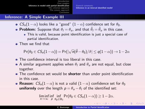
Inference: A Simple Example III

CSn(1−α) looks like a “good” (1−α) confidence set for θ0.Problem: Suppose that θl = θu, and that θl = θu in this case.

This is valid, because point identification is just a special case ofpartial identification.

Then we find that

Pr(θ0 ∈ CSn(1−α)) = Pr(|√

n(θ−θ0)/σ| ≤ q(1−α))→ 1−2α

The confidence interval is too liberal in this case.A similar argument applies when θl and θu are not equal, but closetogether.The confidence set would be shorter than under point identificationin this case.Reason: CSn(1−α) is not a valid (1−α) confidence set for θ0uniformly over the length p = θu−θl of the identified set:

liminfn→∞

infp

infθ0∈ΘI

Pr(θ0 ∈ CSn(1−α))≥ 1−2α.






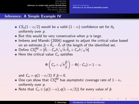
Inference: A Simple Example IV

CSn(1−α/2) would be a valid (1−α) confidence set for θ0uniformly over p.But this would be very conservative when p is large.Imbens and Manski (2004) suggest to adjust the critical value basedon an estimate p = θu− θl of the length of the identified set.Define CS IM

n = [θl −Cnσ/√

n, θu + Cnσ/√

n]Here the critical value Cn satisfies

Φ

(Cn +

√n pσ

)−Φ(−Cn) = 1−α.

and Cn = q(1−α/2) if p = 0.One can show that CS IM

n has asymptotic coverage rate of 1−α,uniformly over p.Note that Cn ∈ (q(1−α),q(1−α/2)) for every value of p.





The two branches of the literatureCHTMoment Inequality Models

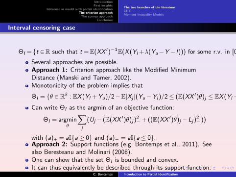
Interval censoring case

ΘI = t ∈R such that t =E(XX ′)−1E(X (Yl +λ(Yu−Y − l))) for some r.v. in [0,1]Several approaches are possible.Approach 1: Criterion approach like the Modified MinimumDistance (Manski and Tamer, 2002).Monotonicity of the problem implies thatΘI = θ ∈ Rk : EX (Yl + Yu)/2−E|Xj |(Yu−Yl )/2≤ (E(XX ′)θ)j ≤ EX (Yl + Yu)/2 +E|Xj |(Yu−Yl )/2.Can write ΘI as the argmin of an objective function:

ΘI = argminθ

∑j

(Uj − (E(XX ′)θ)j)2−+ ((E(XX ′)θ)j −Lj)

2−))

with (a)+ = aIa ≥ 0 and (a)− = aIa ≤ 0.Approach 2: Support functions (e.g. Bontemps et al., 2011). Seealso Beresteanu and Molinari (2008).One can show that the set ΘI is bounded and convex.It can thus equivalently be described through its support function:

δ∗(q,ΘI) = supθ∈ΘI

q′θ.

Bontemps et al. show that support function can be identified fromobservables alone:

Write Σ = E(XX ′)−1 and Xq = q′ΣX andWq = Yl + IXq ≥ 0(Yu−Yl ).Then the support function is identified:

δ∗(q,ΘI ) = E(XqWq)

Moreover, any point θq = ΣE(XWq) is a frontier point of ΘI .






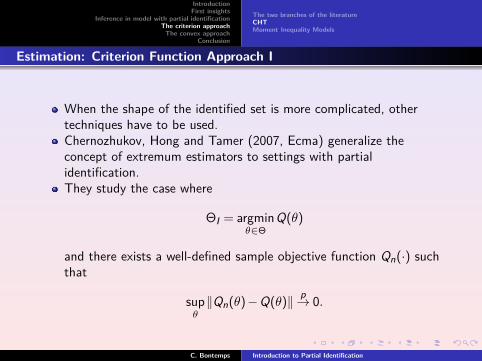
Estimation: Criterion Function Approach I

When the shape of the identified set is more complicated, othertechniques have to be used.Chernozhukov, Hong and Tamer (2007, Ecma) generalize theconcept of extremum estimators to settings with partialidentification.They study the case where

ΘI = argminθ∈Θ

Q(θ)

and there exists a well-defined sample objective function Qn(·) suchthat

supθ‖Qn(θ)−Q(θ)‖ p→ 0.






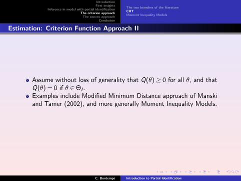
Estimation: Criterion Function Approach II

Assume without loss of generality that Q(θ)≥ 0 for all θ, and thatQ(θ) = 0 if θ ∈ΘI .Examples include Modified Minimum Distance approach of Manskiand Tamer (2002), and more generally Moment Inequality Models.






Estimation: Criterion Function Approach III

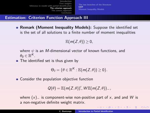
Remark (Moment Inequality Models): Suppose the identified setis the set of all solutions to a finite number of moment inequalities

E(m(Z ,θ))≥ 0,

where ψ is an M-dimensional vector of known functions, andθ0 ∈ RK .The identified set is thus given by

ΘI = θ ∈ RK : E(m(Z ,θ))≥ 0.

Consider the population objective function

Q(θ) = E(m(Z ,θ))′−WE(m(Z ,θ))−,

where (x)− is component-wise non-positive part of x , and and W isa non-negative definite weight matrix.






Estimation: Criterion Function Approach IV

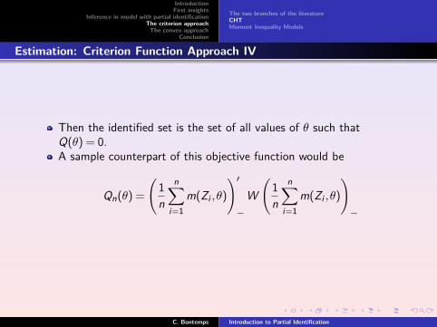
Then the identified set is the set of all values of θ such thatQ(θ) = 0.A sample counterpart of this objective function would be

Qn(θ) =

(1n

n∑i=1

m(Zi ,θ)

)′−

W(

1n

n∑i=1

m(Zi ,θ)

)−






Estimation: Criterion Function Approach V

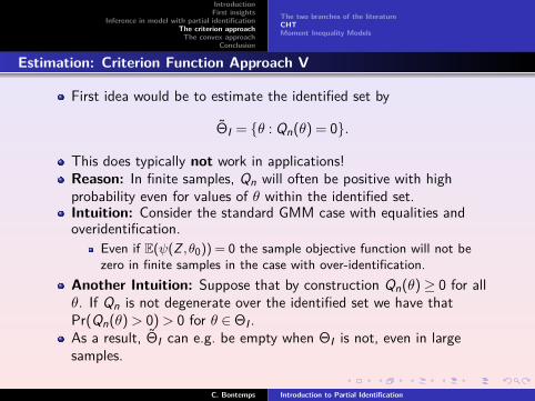
First idea would be to estimate the identified set by

ΘI = θ : Qn(θ) = 0.

This does typically not work in applications!Reason: In finite samples, Qn will often be positive with highprobability even for values of θ within the identified set.Intuition: Consider the standard GMM case with equalities andoveridentification.

Even if E(ψ(Z ,θ0)) = 0 the sample objective function will not bezero in finite samples in the case with over-identification.

Another Intuition: Suppose that by construction Qn(θ)≥ 0 for allθ. If Qn is not degenerate over the identified set we have thatPr(Qn(θ)> 0)> 0 for θ ∈ΘI .As a result, ΘI can e.g. be empty when ΘI is not, even in largesamples.






Estimation: Criterion Function Approach VI

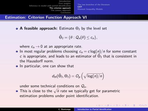
A feasible approach: Estimate ΘI by the level set

ΘI = θ : Qn(θ)≤ cn,

where cn→ 0 at an appropriate rate.In most regular problems choosing cn = c log(n)/n for some constantc is appropriate, and leads to an estimator of ΘI that is consistent inthe Hausdorff norm.In particular, one can show that

dH(ΘI ,ΘI) = Op(√

log(n)/n)

under some technical conditions on Qn.This is close to the

√n rate we typically get for parametric

estimation problems under point identification.






Inference: General Principles I

The role of inferential procedures is to quantify our uncertaintyabout our estimates due to using a finite data set.Inference in partially identified models is still an active area ofresearch.There are many subtle issues that do not appear under pointidentification.We will start with a simple example to illustrate the problems.After that, we turn to are more general framework for inference.






Inference: General Principles II

Suppose we want to compute a confidence set CSn with level 1−α.Problem: What should the confidence set cover (asymptotically)?The entire identified set ΘI?

liminfn→∞

Pr(ΘI ∈ CSn)≥ 1−α.

Or the true parameter value θ0?

liminfn→∞

Pr(θ0 ∈ CSn)≥ 1−α.

Both approaches have been discussed in the literature, and bothhave their place in certain applications.The second notion is more in line with the traditional view of aconfidence interval under point identificationIt is not clear why this intuition should be changed in partiallyidentified models.






Inference: General Principles III

Another problem under partial identification is the uniform validityof confidence sets.We might have that

liminfn→∞

Pr(θ0 ∈ CSn)≥ 1−α.

for one particular DGP.Still, for fixed n the probability Pr(θ0 ∈ CSn) might depend a lot onthe true DGP.It is thus useful to have confidence sets that satisfy

liminfn→∞

infvalid DPGs

Pr(θ0 ∈ CSn)≥ 1−α.

We will illustrate the last point in an example.






Inference: Moment Inequality Models I

We now turn to inference on θ0 in a general setting.We consider models that lead to a system of (unconditional)moment inequalities.Most of our examples can be cast in this framework.Parameter of interest is typically vector valued, and the identified setcan have an arbitrary complicated form.Most of our discussion is based on work of Don Andrews withvarious co-authors.






Inference: Moment Inequality Models II

Model: The true value θ0 satisfies

E(mj(Z ,θ))≥ 0 for j = 1, . . . ,pE(mj(Z ,θ)) = 0 for j = p + 1, . . . ,p + v

Here m(·,θ) = (mj(·,θ), j = 1, . . . ,k) are known real-valued momentfunctions.θ0 may or may not be identified by the moment conditions.Aim: Construct confidence sets for θ0.Can be obtained by inverting a test Tn(θ) for testing H0 : θ = θ0:

CSn = θ ∈Θ : Tn(θ)≤ c(1−α,θ)

Questions: Which test statistic? Which critical value?We will discuss two types of test statistic and three types of criticalvalues.






Inference: Moment Inequality Models III

General setup: consider the sample moment functions

mn(θ) = (mn,1(θ), . . . ,mn,k(θ))′

mn,j(θ) =1n

n∑i=1

mj(Zi ,θ) for j = 1, . . . ,k

Let Σ(θ) be an estimator of the asymptotic variance, Σ(θ), ofn1/2mn(θ).For i.i.d. data we can take

Σ(θ) =1n

n∑i=1

(m(Zi ,θ)− mn(θ))(m(Zi ,θ)− mn(θ))′.






Inference: Moment Inequality Models IV

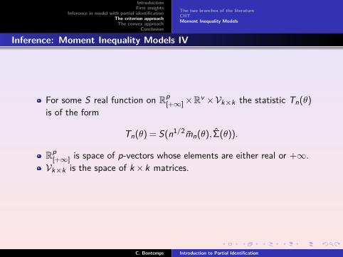
For some S real function on Rp[+∞]×Rv ×Vk×k the statistic Tn(θ)

is of the form

Tn(θ) = S(n1/2mn(θ), Σ(θ)).

Rp[+∞] is space of p-vectors whose elements are either real or +∞.Vk×k is the space of k×k matrices.






Inference: Moment Inequality Models V

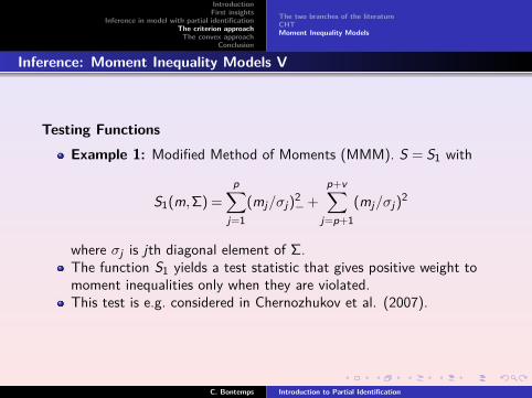
Testing FunctionsExample 1: Modified Method of Moments (MMM). S = S1 with

S1(m,Σ) =

p∑j=1

(mj/σj)2−+

p+v∑j=p+1

(mj/σj)2

where σj is jth diagonal element of Σ.The function S1 yields a test statistic that gives positive weight tomoment inequalities only when they are violated.This test is e.g. considered in Chernozhukov et al. (2007).






Inference: Moment Inequality Models VI

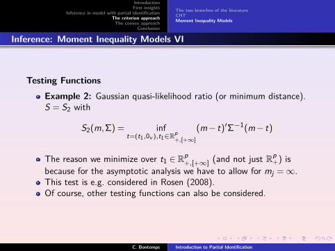
Testing FunctionsExample 2: Gaussian quasi-likelihood ratio (or minimum distance).S = S2 with

S2(m,Σ) = inft=(t1,0v ),t1∈R

p+,[+∞]

(m− t)′Σ−1(m− t)

The reason we minimize over t1 ∈ Rp+,[+∞] (and not just Rp

+) isbecause for the asymptotic analysis we have to allow for mj =∞.This test is e.g. considered in Rosen (2008).Of course, other testing functions can also be considered.






Inference: Moment Inequality Models VII

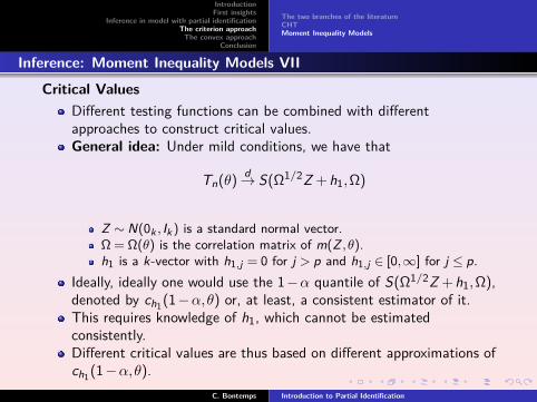
Critical ValuesDifferent testing functions can be combined with differentapproaches to construct critical values.General idea: Under mild conditions, we have that

Tn(θ)d→ S(Ω1/2Z + h1,Ω)

Z ∼ N(0k , Ik ) is a standard normal vector.Ω = Ω(θ) is the correlation matrix of m(Z ,θ).h1 is a k-vector with h1,j = 0 for j > p and h1,j ∈ [0,∞] for j ≤ p.

Ideally, ideally one would use the 1−α quantile of S(Ω1/2Z + h1,Ω),denoted by ch1(1−α,θ) or, at least, a consistent estimator of it.This requires knowledge of h1, which cannot be estimatedconsistently.Different critical values are thus based on different approximations ofch1(1−α,θ).






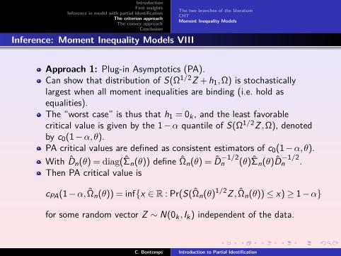
Inference: Moment Inequality Models VIII

Approach 1: Plug-in Asymptotics (PA).Can show that distribution of S(Ω1/2Z + h1,Ω) is stochasticallylargest when all moment inequalities are binding (i.e. hold asequalities).The “worst case” is thus that h1 = 0k , and the least favorablecritical value is given by the 1−α quantile of S(Ω1/2Z ,Ω), denotedby c0(1−α,θ).PA critical values are defined as consistent estimators of c0(1−α,θ).With Dn(θ) = diag(Σn(θ)) define Ωn(θ) = D−1/2

n (θ)Σn(θ)D−1/2n .

Then PA critical value is

cPA(1−α, Ωn(θ)) = infx ∈ R : Pr(S(Ωn(θ)1/2Z , Ωn(θ))≤ x)≥ 1−α

for some random vector Z ∼ N(0k , Ik) independent of the data.






Inference: Moment Inequality Models IX

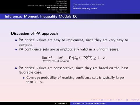
Discussion of PA approachPA critical values are easy to implement, since they are very easy tocompute.PA confidence sets are asymptotically valid in a uniform sense.

liminfn→∞

infvalid DGPs

Pr(θ0 ∈ CSPAn )≥ 1−α

PA critical values are conservative, since they are based on the leastfavorable case.

Coverage probability of resulting confidence sets is typically largerthan 1−α.






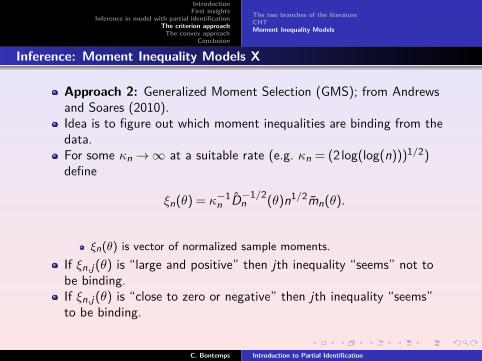
Inference: Moment Inequality Models X

Approach 2: Generalized Moment Selection (GMS); from Andrewsand Soares (2010).Idea is to figure out which moment inequalities are binding from thedata.For some κn→∞ at a suitable rate (e.g. κn = (2 log(log(n)))1/2)define

ξn(θ) = κ−1n D−1/2

n (θ)n1/2mn(θ).

ξn(θ) is vector of normalized sample moments.If ξn,j(θ) is “large and positive” then jth inequality “seems” not tobe binding.If ξn,j(θ) is “close to zero or negative” then jth inequality “seems”to be binding.






Inference: Moment Inequality Models XI

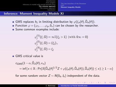
GMS replaces h1 in limiting distribution by ϕ(ξn(θ), Ωn(θ)).Function ϕ= (ϕ1, . . . ,ϕp ,0v ) can be chosen by the researcher.Some common examples include:

ϕ(1)j (ξ,Ω) =∞Iξj > 1 (with 0∞= 0)

ϕ(2)j (ξ,Ω) = (ξj)+

ϕ(3)j (ξ,Ω) = ξj

GMS critical value is

cGMS(1−α, Ωn(θ),κn)

= infx ∈ R : Pr(S(Ωn(θ)1/2Z +ϕ(ξn(θ), Ωn(θ)), Ωn(θ))≤ x)≥ 1−α

for some random vector Z ∼ N(0k , Ik) independent of the data.






Inference: Moment Inequality Models XII

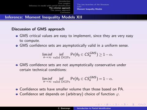
Discussion of GMS approachGMS critical values are easy to implement, since they are very easyto compute.GMS confidence sets are asymptotically valid in a uniform sense.

liminfn→∞

infvalid DGPs

Pr(θ0 ∈ CSGMSn )≥ 1−α.

GMS confidence sets are not asymptotically conservative undercertain technical conditions:

liminfn→∞

infvalid DGPs

Pr(θ0 ∈ CSGMSn ) = 1−α.

Confidence sets have smaller volume than those based on PA.Confidence set depends on (arbitrary) choice of function ϕ.






Inference: Moment Inequality Models XIII

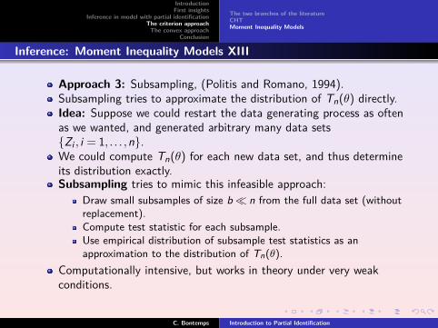
Approach 3: Subsampling, (Politis and Romano, 1994).Subsampling tries to approximate the distribution of Tn(θ) directly.Idea: Suppose we could restart the data generating process as oftenas we wanted, and generated arbitrary many data setsZi , i = 1, . . . ,n.We could compute Tn(θ) for each new data set, and thus determineits distribution exactly.Subsampling tries to mimic this infeasible approach:

Draw small subsamples of size b n from the full data set (withoutreplacement).Compute test statistic for each subsample.Use empirical distribution of subsample test statistics as anapproximation to the distribution of Tn(θ).

Computationally intensive, but works in theory under very weakconditions.






Inference: Moment Inequality Models XIV

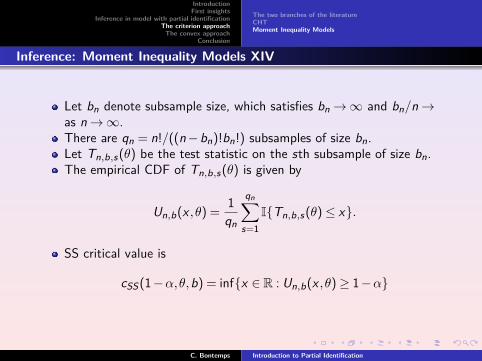
Let bn denote subsample size, which satisfies bn→∞ and bn/n→as n→∞.There are qn = n!/((n−bn)!bn!) subsamples of size bn.Let Tn,b,s(θ) be the test statistic on the sth subsample of size bn.The empirical CDF of Tn,b,s(θ) is given by

Un,b(x ,θ) =1

qn

qn∑s=1

ITn,b,s(θ)≤ x.

SS critical value is

cSS(1−α,θ,b) = infx ∈ R : Un,b(x ,θ)≥ 1−α






Inference: Moment Inequality Models XV

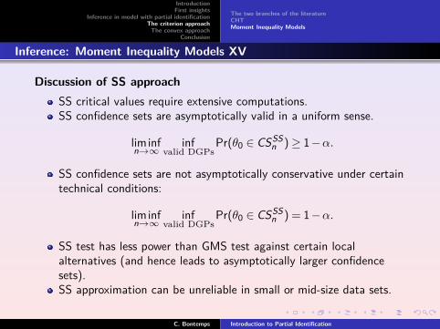
Discussion of SS approachSS critical values require extensive computations.SS confidence sets are asymptotically valid in a uniform sense.

liminfn→∞

infvalid DGPs

Pr(θ0 ∈ CSSSn )≥ 1−α.

SS confidence sets are not asymptotically conservative under certaintechnical conditions:

liminfn→∞

infvalid DGPs

Pr(θ0 ∈ CSSSn ) = 1−α.

SS test has less power than GMS test against certain localalternatives (and hence leads to asymptotically larger confidencesets).SS approximation can be unreliable in small or mid-size data sets.






Inference: Moment Inequality Models XVI

There is a large literature on the advantages and disadvantages ofdifferent approaches to compute test statistics and critical values.Andrews and Jia (2011) recommend using a slightly modified versionof the QLR statistic together with a particular GMS critical value.Bugni et al. (2011) study the properties of the confidence sets underlocal misspecification, finding that

MMM test is more robust than QLR test,PA critical values are more robust than GMS and SS critical values,GMS and SS critical values are equally robust.

There thus seems to be a tradeoff between efficiency and robustness.





Boundedness and convexityThe support functionCriterion viewProjectionCharacterization of the identified setAsymptotic Properties

Using the geometric structure to simplify the inference

The main references are Beresteanu and Molinari (2008),Beresteanu, Molochanov and Molinari (2011), Bontemps, Magnacand Maurin (2012), Kaido and Santos (2013).When the set is convex, one can use the tools of the convex settheory (see Rockafellar, 1970) to propose simple estimators andtesting strategies.Kaido and Santos (2013) estimate an efficiency bound and provethat the natural estimator of the support function is efficientIt is also very simple to propose inference for subset of the vector ofparameters.






No Moment Condition in Surplus

E (zT (xθ− yc)) = E (zT u(z)),u(z) ∈ ±E (yu− yl |z)/2.

The identified set

ΘI = θ : θ= (E (zT x))−1E (zT (y +u(z))),u(z)∈ [−E (yu−yl |z)/2,E (yu−yl |z)/2],

is

Non empty : θ∗ corresponding to u(z) = 0 belongs to B.Bounded : u(z) is uniformly bounded by bounds which are integrable(L2).Convex : Moment conditions are linear and the interval containingu(z) is convex.






Support Function

The dual to the indicator function of a convex set is called its supportfunction, i.e.

δ∗(q | B) = supθ∈B

(qT θ) for all directions, q such that ‖ q ‖= 1.

A convex set can be fully described by its support function, (Rockafellar,1970)

θ ∈ B⇔∀q,‖ q ‖= 1,qT θ ≤ δ∗(q | B).

The support function of a convex and bounded set is bounded anddifferentiable. Its derivative is continuous except at a countable numberof points.






The support function

B

q

βq

qβq






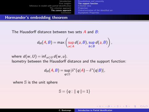
Hormander’s embedding theorem

The Hausdorff distance between two sets A and B:

dH(A,B) = max(

supa∈A

d(a,B), supb∈B

d(a,B)

),

where d(w ,U) = infu∈U d(w ,u).Isometry between the Hausdorff distance and the support function:

dH(A,B) = supq∈S|δ∗(q|A)− δ∗(q|B)|,

where S is the unit sphere

S = q : ‖ q ‖= 1






Inference: The criterion view

Chernozhukov, Hong and Tamer (2007)The identified set B is defined by a criterion:

Q(θ) = 0⇐⇒ θ ∈ B

A natural choice here is:

Q(θ) =

∫S(δ∗(q | B)−qT θ)21δ∗(q|B)< qT θdµ(q)

where µ(q) is a strictly positive measure on the unit sphere S⊂ Rp .






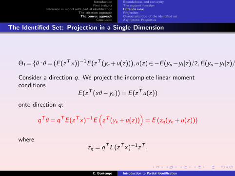
The Identified Set: Projection in a Single Dimension

ΘI = θ : θ= (E (zT x))−1E (zT (yc +u(z))),u(z)∈−E (yu−yl |z)/2,E (yu−yl |z)/2],

Consider a direction q. We project the incomplete linear momentconditions

E (zT (xθ− yc)) = E (zT u(z))

onto direction q:

qT θ = qT E (zT x)−1E(

zT (yc + u(z)))

= E (zq(yc + u(z)))

wherezq = qT E (zT x)−1zT .






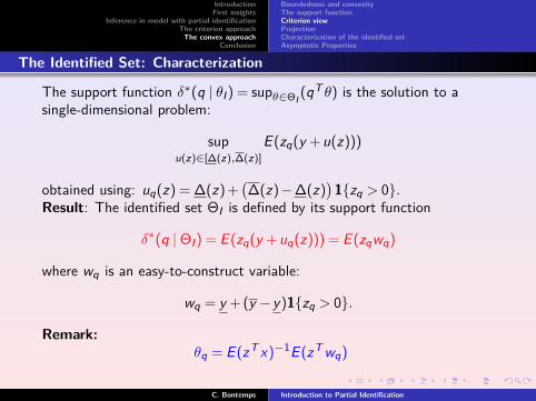
The Identified Set: Characterization

The support function δ∗(q | θI) = supθ∈ΘI (qT θ) is the solution to asingle-dimensional problem:

supu(z)∈[∆(z),∆(z)]

E (zq(y + u(z)))

obtained using: uq(z) = ∆(z) +(∆(z)−∆(z)

)1zq > 0.

Result: The identified set ΘI is defined by its support function

δ∗(q |ΘI) = E (zq(y + uq(z))) = E (zqwq)

where wq is an easy-to-construct variable:

wq = y + (y − y)1zq > 0.

Remark:θq = E (zT x)−1E (zT wq)






Smoothness of the set

If z has full support and his p.d.f. is strictly positive and continuous,the set ΘI is smooth.If z the support is a subset of R and the p.d.f is strictly continuous,ΘI has kinks.If z has mass points, ΘI has exposed faces.If z is discrete ΘI has kinks and exposed faces.






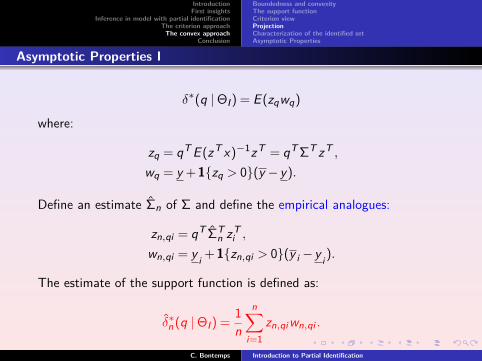
Asymptotic Properties I

δ∗(q |ΘI) = E (zqwq)

where:

zq = qT E (zT x)−1zT = qT ΣT zT ,

wq = y + 1zq > 0(y − y).

Define an estimate Σn of Σ and define the empirical analogues:

zn,qi = qT ΣTn zT

i ,

wn,qi = y i + 1zn,qi > 0(y i − y i ).

The estimate of the support function is defined as:

δ∗n (q |ΘI) =1n

n∑i=1

zn,qi wn,qi .






Asymptotic Properties II

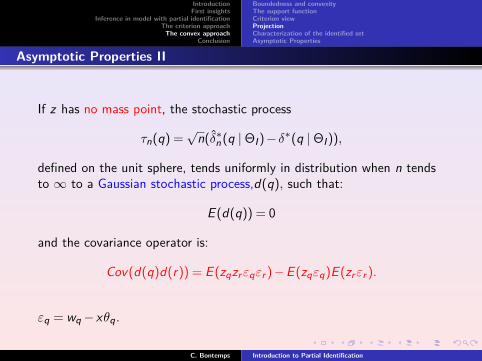
If z has no mass point, the stochastic process

τn(q) =√

n(δ∗n (q |ΘI)− δ∗(q |ΘI)),

defined on the unit sphere, tends uniformly in distribution when n tendsto ∞ to a Gaussian stochastic process,d(q), such that:

E (d(q)) = 0

and the covariance operator is:

Cov(d(q)d(r)) = E (zqzrεqεr )−E (zqεq)E (zrεr ).

εq = wq− xθq.






Tests

Here, we test θ0 ∈ΘI using the support function:

θ0 ∈ΘI ⇐⇒∀q ∈ S, δ∗(q |ΘI)−qT θ0 ≥ 0

For a frontier point, θ0 ∈ ∂ΘI , there exists at least one direction q0 forwhich the previous expression binds with equality:

∃q0 ∈ S, δ∗(q0 |ΘI) = qT0 θ0

If ΘI is strictly convex, q0 is unique.






Test Procedure for θ0 ∈ΘI I

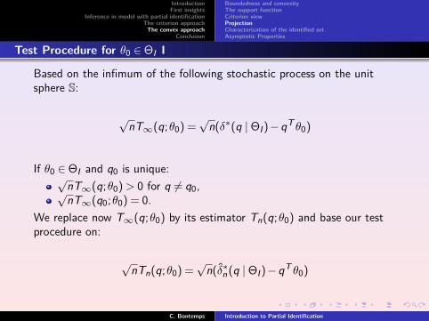
Based on the infimum of the following stochastic process on the unitsphere S:

√nT∞(q;θ0) =

√n(δ∗(q |ΘI)−qT θ0)

If θ0 ∈ΘI and q0 is unique:√

nT∞(q;θ0)> 0 for q 6= q0,√nT∞(q0;θ0) = 0.

We replace now T∞(q;θ0) by its estimator Tn(q;θ0) and base our testprocedure on:

√nTn(q;θ0) =

√n(δ∗n (q |ΘI)−qT θ0)






Test Procedure for θ0 ∈ΘI II

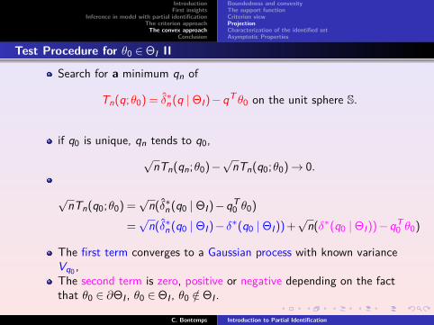
Search for a minimum qn of

Tn(q;θ0) = δ∗n (q |ΘI)−qT θ0 on the unit sphere S.

if q0 is unique, qn tends to q0,√

nTn(qn;θ0)−√

nTn(q0;θ0)→ 0.

√nTn(q0;θ0) =

√n(δ∗n (q0 |ΘI)−qT

0 θ0)

=√

n(δ∗n (q0 |ΘI)− δ∗(q0 |ΘI)) +√

n(δ∗(q0 |ΘI))−qT0 θ0)

The first term converges to a Gaussian process with known varianceVq0 ,The second term is zero, positive or negative depending on the factthat θ0 ∈ ∂ΘI , θ0 ∈ΘI , θ0 /∈ΘI .






Summary

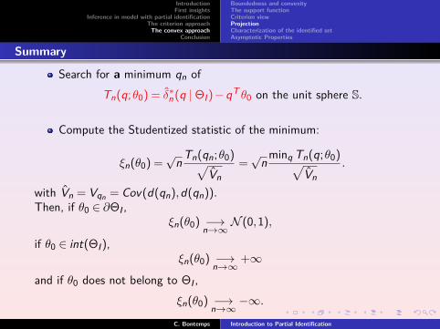
Search for a minimum qn ofTn(q;θ0) = δ∗n (q |ΘI)−qT θ0 on the unit sphere S.

Compute the Studentized statistic of the minimum:

ξn(θ0) =√

n Tn(qn;θ0)√Vn

=√

n minq Tn(q;θ0)√Vn

.

with Vn = Vqn = Cov(d(qn),d(qn)).Then, if θ0 ∈ ∂ΘI ,

ξn(θ0) −→n→∞

N (0,1),

if θ0 ∈ int(ΘI),ξn(θ0) −→

n→∞+∞

and if θ0 does not belong to ΘI ,ξn(θ0) −→

n→∞−∞.





In many examples, point identification is ruled out because someinformation is missing.If one can bound this information, a set can be estimated.Despite the huge number of theoretical contributions, a fewempirical applications only (see next course).There is still theoretical and empirical work to do.


Documents

Introduction to Partial Identification - Paul Scottptscott.com/teaching/tse_eio_2014/partial-identification-overview.pdf · Introduction First insights Inference in model with partial