Embed Size (px)
Citation preview
Introduction to QCD and Jet I
Bo-Wen Xiao
Pennsylvania State Universityand Institute of Particle Physics, Central China Normal University
Jet Summer SchoolMcGill June 2012
1 / 38
Overview of the Lectures
Lecture 1 - Introduction to QCD and JetQCD basicsSterman-Weinberg Jet in e+e− annihilationCollinear Factorization and DGLAP equationBasic ideas of kt factorization
Lecture 2 - kt factorization and Dijet Processes in pA collisionskt Factorization and BFKL equationNon-linear small-x evolution equations.Dijet processes in pA collisions (RHIC and LHC related physics)
Lecture 3 - kt factorization and Higher Order Calculations in pA collisions
No much specific exercise. 1. filling gaps of derivation; 2. Reading materials.
2 / 38
Outline
1 Introduction to QCD and JetQCD BasicsSterman-Weinberg JetsCollinear Factorization and DGLAP equationTransverse Momentum Dependent (TMD or kt) Factorization
3 / 38
References:
R.D. Field, Applications of perturbative QCD A lot of detailed examples.
R. K. Ellis, W. J. Stirling and B. R. Webber, QCD and Collider Physics
CTEQ, Handbook of Perturbative QCD
CTEQ website.
John Collins, The Foundation of Perturbative QCD Includes a lot new development.
Yu. L. Dokshitzer, V. A. Khoze, A. H. Mueller and S. I. Troyan, Basics of PerturbativeQCD More advanced discussion on the small-x physics.
S. Donnachie, G. Dosch, P. Landshoff and O. Nachtmann, Pomeron Physics and QCD
V. Barone and E. Predazzi, High-Energy Particle Diffraction
4 / 38
Introduction to QCD and Jet QCD Basics
QCD
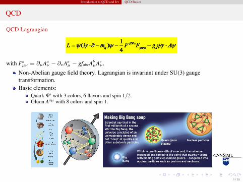
QCD Lagrangian
with Faµν = ∂µAa
ν − ∂νAaµ − gfabcAb
µAcν .
Non-Abelian gauge field theory. Lagrangian is invariant under SU(3) gaugetransformation.Basic elements:
Quark Ψi with 3 colors, 6 flavors and spin 1/2.Gluon Aaµ with 8 colors and spin 1.
5 / 38
Introduction to QCD and Jet QCD Basics
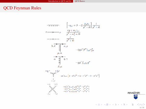
QCD Feynman Rules
6 / 38
Introduction to QCD and Jet QCD Basics
Color Structure
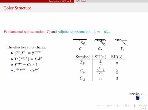
Fundamental representation: Taij and Adjoint representation: ta
bc = −ifabc
The effective color charge:[Ta, Tb] = if abcTc
Tr(TaTb) = TFδ
ab
TaTa = CF × 1
f abcf abd = CAδcd
7 / 38
Introduction to QCD and Jet QCD Basics
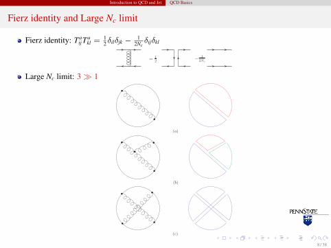
Fierz identity and Large Nc limit
Fierz identity: TaijT
akl = 1
2δilδjk − 12Ncδijδkl
= 12
− 12Nc
Large Nc limit: 3 1
(a)
(b)
(c)
8 / 38
Introduction to QCD and Jet QCD Basics
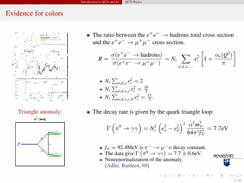
Evidence for colors
The ratio between the e+e− → hadrons total cross sectionand the e+e− → µ+µ− cross section.
R =σ(e+e− → hadrons)σ(e+e− → µ+µ−)
= Nc
∑u,d,s,...
e2i
[1 +
αs(Q2)
π
]
Nc∑
u,d,s e2i = 2
Nc∑
u,d,s,c e2i = 10
3Nc∑
u,d,s,c,b e2i = 11
3 .
Triangle anomaly: The decay rate is given by the quark triangle loop:
Γ(π0 → γγ
)= N2
c
(e2
u − e2d
)2 α2m3π
64π3f 2π
= 7.7eV
fπ = 92.4MeV is π− → µ−ν decay constant.The data give Γ
(π0 → γγ
)= 7.7± 0.6eV.
Nonrenormalization of the anomaly.[Adler, Bardeen, 69]
9 / 38
Introduction to QCD and Jet QCD Basics
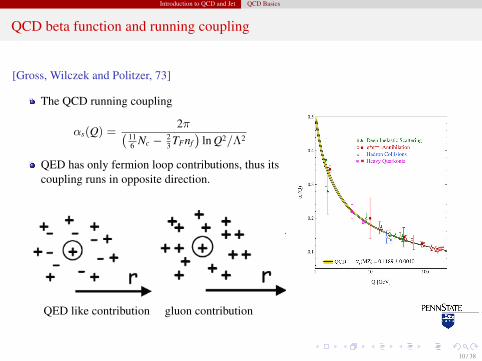
QCD beta function and running coupling
[Gross, Wilczek and Politzer, 73]
The QCD running coupling
αs(Q) =2π( 11
6 Nc − 23 TFnf
)ln Q2/Λ2
QED has only fermion loop contributions, thus itscoupling runs in opposite direction.
QED like contribution gluon contribution
10 / 38
Introduction to QCD and Jet QCD Basics
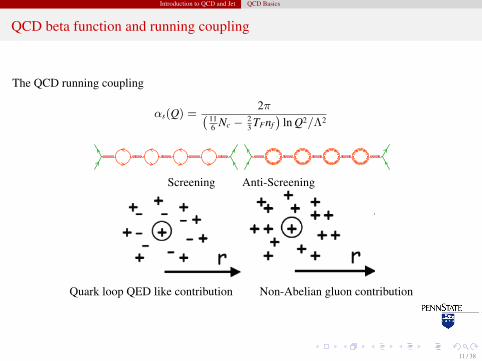
QCD beta function and running coupling
The QCD running coupling
αs(Q) =2π( 11
6 Nc − 23 TFnf
)ln Q2/Λ2
Testing QCD!QCD reminder!Confinement!How to test QCD?!Factorization
Parton model
Gluon saturation
Phenomenology of saturation
CERN
François Gelis – 2007 Lecture I / III – School on QCD, low-x physics, saturation and diffraction, Copanello, July 2007 - p. 7/40
Asymptotic freedom" Running coupling : αs = g2/4π
αs(r) =2πNc
(11Nc − 2Nf ) log(1/rΛQCD)
" The effective charge seen at large distance is screened byfermionic fluctuations (as in QED)
" But gluonic vacuum fluctuations produce an anti-screening(because of the non-abelian nature of their interactions)
" As long as Nf <11Nc/2 = 16.5, the gluons win...
Screening Anti-Screening
Quark loop QED like contribution Non-Abelian gluon contribution
11 / 38
Introduction to QCD and Jet QCD Basics
Brief History of QCD beta function
1954 Yang and Mills introduced the non-Abelian gauge thoery.
1965 Vanyashin and Terentyev calculated the beta function for a massive charged vectorfield theory.
1971 ’t Hooft computed the one-loop beta function for SU(3) gauge theory, but his advisor(Veltman) told him it wasn’t interesting.
1972 Gell-Mann proposed that strong interaction is described by SU(3) gauge theory,namely QCD.
1973 Gross and Wilczek, and independently Politzer, computed the 1-loop beta-functionfor QCD.
1999 ’t Hooft and Veltman received the 1999 Nobel Prize for proving the renormalizabilityof QCD.
2004 Gross, Wilczek and Politzer received the Nobel Prize.
12 / 38
Introduction to QCD and Jet QCD Basics
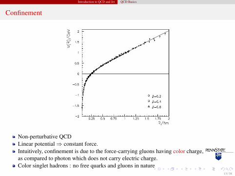
Confinement
Non-perturbative QCDLinear potential⇒ constant force.Intuitively, confinement is due to the force-carrying gluons having color charge,as compared to photon which does not carry electric charge.Color singlet hadrons : no free quarks and gluons in nature
13 / 38
Introduction to QCD and Jet QCD Basics
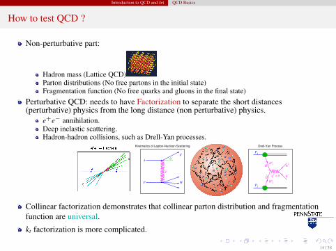
How to test QCD ?
Non-perturbative part:
Hadron mass (Lattice QCD)Parton distributions (No free partons in the initial state)Fragmentation function (No free quarks and gluons in the final state)
Perturbative QCD: needs to have Factorization to separate the short distances(perturbative) physics from the long distance (non perturbative) physics.
e+e− annihilation.Deep inelastic scattering.Hadron-hadron collisions, such as Drell-Yan processes.
Kinematics of Lepton-Nucleon Scattering
k
k′
θ
q
P W
Drell-Yan Process
P1
xP1
q2 > 0
P2
x_P
2
µ+
µ−
Q
Q−
Collinear factorization demonstrates that collinear parton distribution and fragmentationfunction are universal.
kt factorization is more complicated.
14 / 38
Introduction to QCD and Jet Sterman-Weinberg Jets
e+e− annihilation
p1
p2
p3
q
q
gγ∗ γ∗
p2
q
p3
p1
q
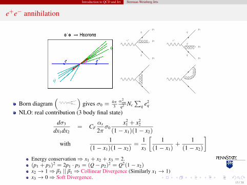
Born diagram( )
gives σ0 = 4π3α2
emq2 Nc
∑q e2
q
NLO: real contribution (3 body final state)
dσ3
dx1dx2= CF
αs
2πσ0
x21 + x2
2
(1− x1)(1− x2)
with1
(1− x1)(1− x2)=
1x3
[1
(1− x1)+
1(1− x2)
]Energy conservation⇒ x1 + x2 + x3 = 2.(p1 + p3)2 = 2p1 · p3 = (Q− p2)2 = Q2(1− x2)x2 → 1⇒~p3 ||~p1⇒ Collinear Divergence (Similarly x1 → 1)x3 → 0⇒ Soft Divergence.
15 / 38
Introduction to QCD and Jet Sterman-Weinberg Jets
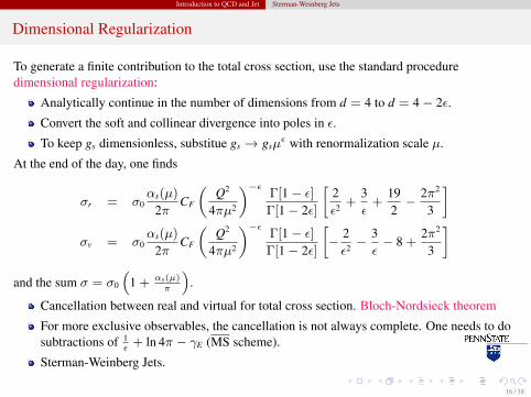
Dimensional Regularization
To generate a finite contribution to the total cross section, use the standard proceduredimensional regularization:
Analytically continue in the number of dimensions from d = 4 to d = 4− 2ε.
Convert the soft and collinear divergence into poles in ε.
To keep gs dimensionless, substitue gs → gsµε with renormalization scale µ.
At the end of the day, one finds
σr = σ0αs(µ)
2πCF
(Q2
4πµ2
)−εΓ[1− ε]Γ[1− 2ε]
[2ε2 +
3ε
+192− 2π2
3
]σv = σ0
αs(µ)
2πCF
(Q2
4πµ2
)−εΓ[1− ε]Γ[1− 2ε]
[− 2ε2 −
3ε− 8 +
2π2
3
]and the sum σ = σ0
(1 + αs(µ)
π
).
Cancellation between real and virtual for total cross section. Bloch-Nordsieck theorem
For more exclusive observables, the cancellation is not always complete. One needs to dosubtractions of 1
ε+ ln 4π − γE (MS scheme).
Sterman-Weinberg Jets.
16 / 38
Introduction to QCD and Jet Sterman-Weinberg Jets
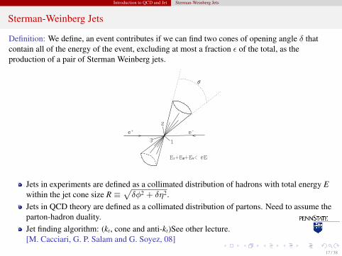
Sterman-Weinberg Jets
Definition: We define, an event contributes if we can find two cones of opening angle δ thatcontain all of the energy of the event, excluding at most a fraction ε of the total, as theproduction of a pair of Sterman Weinberg jets.
Fig. 11: Sterman–Weinberg jets.
All the Born cross section contributes to the Sterman–Weinberg cross section, irrespective of thevalue of and (fig. 12a).
All the virtual cross section contributes to the Sterman–Weinberg cross section, irrespective of thevalue of and (fig. 12b).
The real cross section, with one gluon emission, when the energy of the emitted gluon is limitedby (fig. 12c), contributes to the Sterman–Weinberg cross section.
The real cross section, when , when the emission angle with respect to the quark (orantiquark) is less than (fig. 12d), contributes to the Sterman–Weinberg cross section.
The various divergent contributions are given formally by
Born (74)
Virtual (75)
Real (c) (76)
Real (d) (77)
Observe that the expression of the virtual term is fixed by the fact that it has to cancel the total of the realcontribution. Since we are looking only at divergent terms, and since the virtual term is independent ofand , the expression (75) is fully adequate for our purposes. Summing all terms we get
Born Virtual Real (a) Real (b)
(78)
which is finite, as long as and are finite. Furthermore, as long as and are not too small, we findthat the fraction of events with two Sterman-Weinberg jets is 1, up to a correction of order .
20
Jets in experiments are defined as a collimated distribution of hadrons with total energy Ewithin the jet cone size R ≡
√δφ2 + δη2.
Jets in QCD theory are defined as a collimated distribution of partons. Need to assume theparton-hadron duality.Jet finding algorithm: (kt, cone and anti-kt)See other lecture.[M. Cacciari, G. P. Salam and G. Soyez, 08]
17 / 38
Introduction to QCD and Jet Sterman-Weinberg Jets
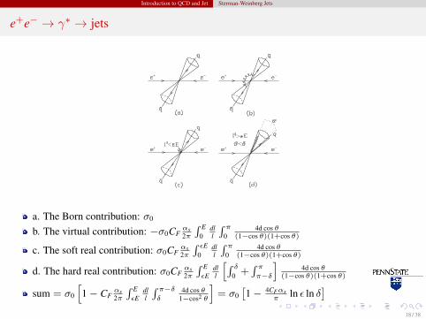
e+e− → γ∗ → jets
Fig. 12: Contributions to the Sterman–Weinberg cross–section. Born: (a), virtual: (b), real emission: (c) and (d).
Now we are ready to perform a qualitative step: we interpret the Sterman-Weinberg cross section,computed using the language of quarks and gluons, as a cross section for producing hadrons. Thanks tothis qualitative step, we make the following prediction: at high energy, most events have a large fractionof the energy contained in opposite cones, that is to say most events are two jet events. As the energybecomes larger becomes smaller. Therefore we can use smaller values of and to define our jets.Thus, at higher energies jets become thinner.
It should be clear now to the reader that, by the same reasoning followed so far, the angulardistribution of the jets will be very close, at high energy, to the angular distribution one computes usingthe Born cross section, that is to say, the typical distribution. These predictions have beenverified experimentally since a long time.
4.2 A comparison with QEDThe alert reader will have probably realized that the discussion given in this section could have beengiven as well with respect to electrodynamics. In fact, the Feynman diagrams we have considered arepresent also in electrodynamic processes, like , and they differ from the QCD graphsonly by the color factor. Thus, from the previous discussion, we would infer that Sterman-Weinbergjets in electrodynamic processes at high energy do not depend upon long distance features of the theory.For example, they become independent from the mass when . Also in electrodynamics, thecross section for producing a pair plus a photon is divergent, as is divergent the cross section forproducing the pair without any photon. In many books on quantum electrodynamics these divergencesare discussed, and it is shown that a resolution parameter for the minimum energy of a photon is neededin order to have finite cross section order by order in perturbation theory. In electrodynamics, we cango even farther, and prove that by resumming the whole tower of divergent graphs, the infinite negativevirtual correction to the production of a pair with no photons exponentiates, and gives a zero crosssection. In other words, as it is well known, it is impossible to produce charged pairs without producing
21
a. The Born contribution: σ0
b. The virtual contribution: −σ0CFαs2π
∫ E0
dll
∫ π0
4d cos θ(1−cos θ)(1+cos θ)
c. The soft real contribution: σ0CFαs2π
∫ εE0
dll
∫ π0
4d cos θ(1−cos θ)(1+cos θ)
d. The hard real contribution: σ0CFαs2π
∫ EεE
dll
[∫ δ0 +
∫ ππ−δ
]4d cos θ
(1−cos θ)(1+cos θ)
sum = σ0
[1− CF
αs2π
∫ EεE
dll
∫ π−δδ
4d cos θ1−cos2 θ
]= σ0
[1− 4CFαs
πln ε ln δ
]18 / 38
Introduction to QCD and Jet Sterman-Weinberg Jets
Infrared Safety
We have encountered two kinds of divergences: collinear divergence and soft divergence.Both of them are of the Infrared divergence type.That is to say, they both involve longdistance.
According to uncertainty principle, soft↔ long distance;Also one needs an infinite time in order to specify accurately the particle momenta, andtherefore their directions.
For a suitable defined inclusive observable (e.g., σe+e−→hadrons), there is a cancellationbetween the soft and collinear singularities occurring in the real and virtual contributions.Kinoshita-Lee-Nauenberg theorem
Any new observables must have a definition which does not distinguish between
parton↔ parton + soft gluonparton↔ two collinear partons
Observables that respect the above constraint are called infrared safe observables. Infraredsafety is a requirement that the observable is calculable in pQCD.
Other infrared safe observables, for example, Thrust: T = max∑
i |pi·n|∑i |pi|
...
19 / 38
Introduction to QCD and Jet Sterman-Weinberg Jets
Fragmentation function
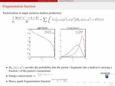
Factorization of single inclusive hadron production:
1σ0
dσ(e+e− → h + X)
dx=∑
i
∫ 1
xCi
(z, αs(µ
2), s/µ2)
Dh/i(x/z, µ2) +O(1/s)
Dh/i(x/z, µ2) encodes the probability that the parton i fragments into a hadron h carrying afraction z of the parton’s momentum.
Energy conservation⇒
2 17. Fragmentation functions in e+e−, ep and pp collisions
0.00050.0010.0020.0050.010.020.050.10.20.5
125
102050
100200500
F T,L(
x)
!s=91 GeV
LEP FT
LEP FL
0 0.1 0.2 0.3 0.4 0.5 0.6 0.7 0.8 0.9 1x
F A(x
)
-0.8-0.4
00.40.8
LEP FA
Figure 17.1: LEP1 measurements of total transverse (FT ), longitudinal (FL),and asymmetric (FA) fragmentation functions [6–8]. Data points with relative errorsgreater than 100% are omitted.
probability that the parton i fragments into a hadron h carrying a fraction z of theparton’s momentum. Beyond the leading order (LO) of perturbative QCD these universalfunctions are factorization-scheme dependent, with ‘reasonable’ scheme choices retainingcertain quark-parton-model (QPM) constraints such as the momentum sum rule
∑
h
∫ 1
0dz z Dh
i (z, µ2) = 1 . (17.3)
The dependence of the functions Dhi on the factorization (or fragmentation) scale µ2 (in
Eq. (17.2) and below identified with the renormalization scale) is discussed in Section17.2.
The second ingredient in Eq. (17.2), and analogous expressions for the functionsFT,L,A , are the observable-dependent coefficient functions Ci. At the zeroth order in the
February 16, 2012 14:07
Heavy quark fragmentation function: .20 / 38
Introduction to QCD and Jet Collinear Factorization and DGLAP equation
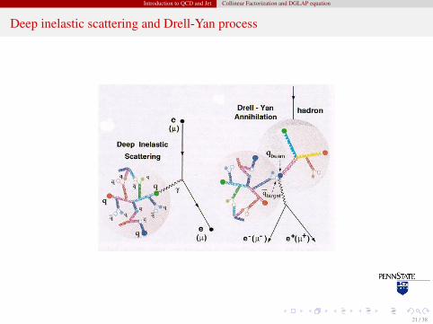
Deep inelastic scattering and Drell-Yan process
21 / 38
Introduction to QCD and Jet Collinear Factorization and DGLAP equation
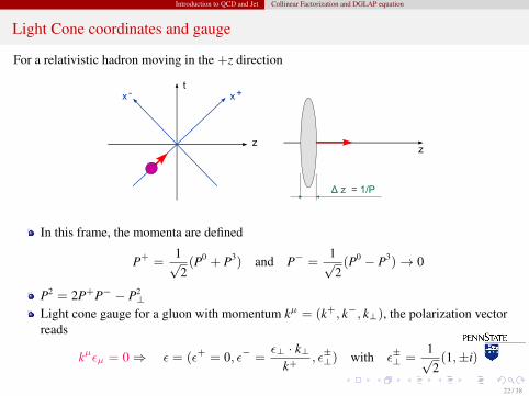
Light Cone coordinates and gauge
For a relativistic hadron moving in the +z direction
Motivation
Dipole picture for DIS
Non–linear evolution: BK!Bremsstrahlung!BFKL Evolution! Light Cone!Dipole splitting!Dipole evolution!Balitsky equation!BK equation
SCHOOL ON QCD, LOW X PHYSICS, SATURATION AND DIFFRACTION: Copanello (Calabria, Italy), July 1 - 14 2007 Non–linear evolution & Gluon saturation in QCD at high energy (I) – p. 25
Light Cone notations & Kinematics" The hadron moves in the positive z direction, with v ! c = 1
" Longitudinal momentum P " M =⇒ P µ = (E ≈ P, 0, 0, P )
P+ ≡ 1√2(E + P ) !
√2P , P − ≡ 1√
2(E − P ) ! 0
" Even for the quantum system, the wavefunction is stronglylocalized near x− = 0 (“pancake”)
∆x− ∼ 1
P+∼ 1
γM) 1
M
In this frame, the momenta are defined
P+ =1√2
(P0 + P3) and P− =1√2
(P0 − P3)→ 0
P2 = 2P+P− − P2⊥
Light cone gauge for a gluon with momentum kµ = (k+, k−, k⊥), the polarization vectorreads
kµεµ = 0⇒ ε = (ε+ = 0, ε− =ε⊥ · k⊥
k+, ε±⊥) with ε±⊥ =
1√2
(1,±i)
22 / 38
Introduction to QCD and Jet Collinear Factorization and DGLAP equation
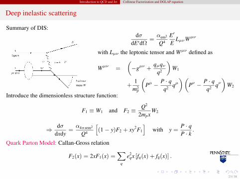
Deep inelastic scattering
Summary of DIS:dσ
dE′dΩ=αem2
Q4
E′
ELµνWµν
with Lµν the leptonic tensor and Wµν defined as
Wµν =
(−gµν +
qµqνq2
)W1
+1
m2p
(Pµ − P · q
q2 qµ)(
Pν − P · qq2 qν
)W2
Introduce the dimensionless structure function:
F1 ≡ W1 and F2 ≡ Q2
2mpxW2
⇒ dσdxdy
=α4πsem2
Q4
[(1− y)F2 + xy2F1
]with y =
P · qP · k .
Quark Parton Model: Callan-Gross relation
F2(x) = 2xF1(x) =∑
q
e2qx [fq(x) + fq(x)] .
23 / 38

Introduction to QCD and Jet Collinear Factorization and DGLAP equation
Callan-Gross relation
The relation (FL = F2 − 2xF1) follows from the fact that a spin- 12 quark cannot absorb a
longitudinally polarized vector boson.In contrast, spin-0 quark cannot absorb transverse bosons and so would give F1 = 0.
24 / 38
Introduction to QCD and Jet Collinear Factorization and DGLAP equation
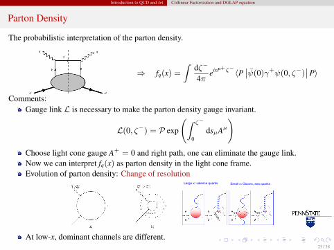
Parton Density
The probabilistic interpretation of the parton density.
⇒ fq(x) =
∫dζ−
4πeixP+ζ−〈P
∣∣ψ(0)γ+ψ(0, ζ−)∣∣P〉
Comments:Gauge link L is necessary to make the parton density gauge invariant.
L(0, ζ−) = P exp
(∫ ζ−
0dsµAµ
)Choose light cone gauge A+ = 0 and right path, one can eliminate the gauge link.Now we can interpret fq(x) as parton density in the light cone frame.Evolution of parton density: Change of resolution
13J.Pawlowski / U. Uwer
Advanced Particle Physics: VII. Quantum Chromodynamics
QCD explains observed scaling violation
Large x: valence quarks Small x: Gluons, sea quarks
Q2 F2 for fixed x Q2 F2 for fixed x
Scaling violation is one of the clearest manifestation of radiative effect predicted by QCD.
Quantitative description of scaling violation
)()()()( 21
0
22 xqexdxqexxF i
ii
iii
P
Quark Parton Model
QCD
P
x/xz
)log()(P2
~
)(P2
~
20
2
2
2
2
20
Qz
kdkz
s
Q
T
Ts
Tkk,
20
21
0
222 log)(P
2)1()(),(
Qxxq
dexQxF qq
s
iii
Pqq probability of a quark to emit gluon and becoming a quark with momentum reduced by fraction z.
0 cutoff parameter
MQx
2
2
)(1
)( xa
ax
x
x x
At low-x, dominant channels are different.25 / 38
Introduction to QCD and Jet Collinear Factorization and DGLAP equation
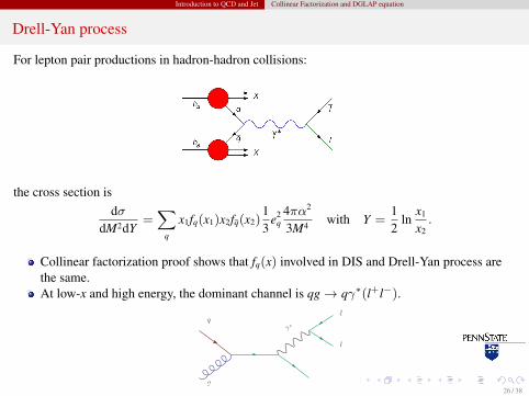
Drell-Yan process
For lepton pair productions in hadron-hadron collisions:
the cross section isdσ
dM2dY=∑
q
x1fq(x1)x2fq(x2)13
e2q
4πα2
3M4 with Y =12
lnx1
x2.
Collinear factorization proof shows that fq(x) involved in DIS and Drell-Yan process arethe same.At low-x and high energy, the dominant channel is qg→ qγ∗(l+l−).
g
qγ∗
l
l
26 / 38

Introduction to QCD and Jet Collinear Factorization and DGLAP equation
Splitting function
P0qq(ξ) =
1 + ξ2
(1− ξ)++
32δ(1− ξ),
P0gq(ξ) =
1ξ
[1 + (1− ξ)2
],
P0qg(ξ) =
[(1− ξ)2 + ξ2
],
P0gg(ξ) = 2
[ξ
(1− ξ)+
+1− ξξ
+ ξ(1− ξ)]
+
(116− 2Nf TR
3Nc
)δ(1− ξ).
ξ = z = xy .∫ 1
0dξf (ξ)
(1−ξ)+=∫ 1
0dξ[f (ξ)−f (1)]
1−ξ ⇒∫ 1
0dξ
(1−ξ)+= 0
27 / 38
Introduction to QCD and Jet Collinear Factorization and DGLAP equation
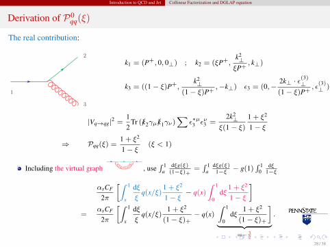
Derivation of P0qq(ξ)
The real contribution:
1
2
3
k1 = (P+, 0, 0⊥) ; k2 = (ξP+,k2⊥
ξP+, k⊥)
k3 = ((1− ξ)P+,k2⊥
(1− ξ)P+,−k⊥) ε3 = (0,−
2k⊥ · ε(3)⊥
(1− ξ)P+, ε
(3)⊥ )
|Vq→qg|2 =12
Tr (/k2γµ/k1γν)∑
ε∗µ3 εν3 =2k2⊥
ξ(1− ξ)1 + ξ2
1− ξ
⇒ Pqq(ξ) =1 + ξ2
1− ξ(ξ < 1)
Including the virtual graph , use∫ 1
adξg(ξ)
(1−ξ)+=∫ 1
adξg(ξ)
1−ξ − g(1)∫ 1
0dξ
1−ξ
αsCF
2π
[∫ 1
x
dξξ
q(x/ξ)1 + ξ2
1− ξ− q(x)
∫ 1
0dξ
1 + ξ2
1− ξ
]=
αsCF
2π
[∫ 1
x
dξξ
q(x/ξ)1 + ξ2
(1− ξ)+− q(x)
∫ 1
0dξ
1 + ξ2
(1− ξ)+
]︸ ︷︷ ︸
=− 32
.
28 / 38
Introduction to QCD and Jet Collinear Factorization and DGLAP equation
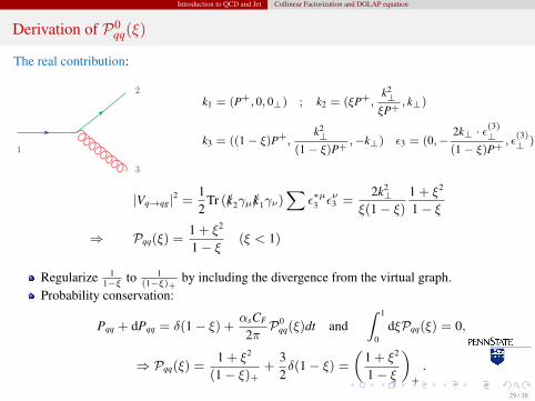
Derivation of P0qq(ξ)
The real contribution:
1
2
3
k1 = (P+, 0, 0⊥) ; k2 = (ξP+,k2⊥
ξP+, k⊥)
k3 = ((1− ξ)P+,k2⊥
(1− ξ)P+,−k⊥) ε3 = (0,−
2k⊥ · ε(3)⊥
(1− ξ)P+, ε
(3)⊥ )
|Vq→qg|2 =12
Tr (/k2γµ/k1γν)∑
ε∗µ3 εν3 =2k2⊥
ξ(1− ξ)1 + ξ2
1− ξ
⇒ Pqq(ξ) =1 + ξ2
1− ξ (ξ < 1)
Regularize 11−ξ to 1
(1−ξ)+by including the divergence from the virtual graph.
Probability conservation:
Pqq + dPqq = δ(1− ξ) +αsCF
2πP0
qq(ξ)dt and∫ 1
0dξPqq(ξ) = 0,
⇒ Pqq(ξ) =1 + ξ2
(1− ξ)++
32δ(1− ξ) =
(1 + ξ2
1− ξ
)+
.
29 / 38
Introduction to QCD and Jet Collinear Factorization and DGLAP equation
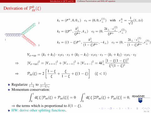
Derivation of P0gg(ξ)
1
2
3
k1 = (P+, 0, 0⊥) ε1 = (0, 0, ε(1)⊥ ) with ε±⊥ =
1√
2(1,±i)
k2 = (ξP+,k2⊥
ξP+, k⊥) ε2 = (0,
2k⊥ · ε(2)⊥
ξP+, ε
(2)⊥ )
k3 = ((1− ξ)P+,k2⊥
(1− ξ)P+,−k⊥) ε3 = (0,−
2k⊥ · ε(3)⊥
(1− ξ)P+, ε
(3)⊥ )
Vg→gg = (k1 + k3) · ε2ε1 · ε3 + (k2 − k3) · ε1ε2 · ε3 − (k1 + k2) · ε3ε1 · ε2
⇒ |Vg→gg|2 = |V+++|2 + |V+−+|2 + |V++−|2 = 4k2⊥
[1− ξ(1− ξ)]2
ξ2(1− ξ)2
⇒ Pgg(ξ) = 2[
1− ξξ
+ξ
1− ξ + ξ(1− ξ)]
(ξ < 1)
Regularize 11−ξ to 1
(1−ξ)+Momentum conservation:∫ 1
0dξ ξ [Pqq(ξ) + Pgq(ξ)] = 0
∫ 1
0dξ ξ [2Pqg(ξ) + Pgg(ξ)] = 0,
⇒ the terms which is proportional to δ(1− ξ).HW: derive other splitting functions. 30 / 38
Introduction to QCD and Jet Collinear Factorization and DGLAP equation
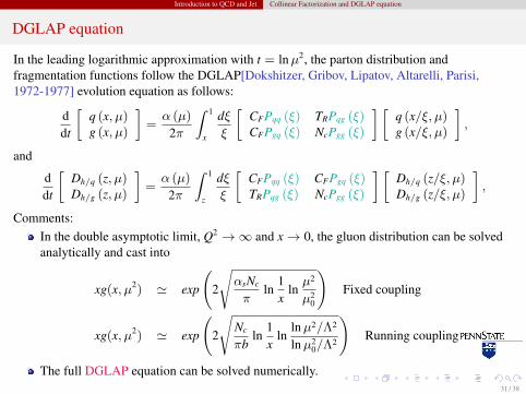
DGLAP equation
In the leading logarithmic approximation with t = lnµ2, the parton distribution andfragmentation functions follow the DGLAP[Dokshitzer, Gribov, Lipatov, Altarelli, Parisi,1972-1977] evolution equation as follows:
ddt
[q (x, µ)g (x, µ)
]=α (µ)
2π
∫ 1
x
dξξ
[CFPqq (ξ) TRPqg (ξ)CFPgq (ξ) NcPgg (ξ)
] [q (x/ξ, µ)g (x/ξ, µ)
],
and
ddt
[Dh/q (z, µ)Dh/g (z, µ)
]=α (µ)
2π
∫ 1
z
dξξ
[CFPqq (ξ) CFPgq (ξ)TRPqg (ξ) NcPgg (ξ)
] [Dh/q (z/ξ, µ)Dh/g (z/ξ, µ)
],
Comments:In the double asymptotic limit, Q2 →∞ and x→ 0, the gluon distribution can be solvedanalytically and cast into
xg(x, µ2) ' exp
(2
√αsNc
πln
1x
lnµ2
µ20
)Fixed coupling
xg(x, µ2) ' exp
(2
√Nc
πbln
1x
lnlnµ2/Λ2
lnµ20/Λ
2
)Running coupling
The full DGLAP equation can be solved numerically.31 / 38
Introduction to QCD and Jet Collinear Factorization and DGLAP equation
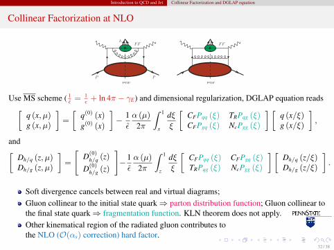
Collinear Factorization at NLO
PDF PDF
FF FF
P P
h
Use MS scheme ( 1ε
= 1ε
+ ln 4π − γE) and dimensional regularization, DGLAP equation reads[q (x, µ)g (x, µ)
]=
[q(0) (x)
g(0) (x)
]− 1ε
α (µ)
2π
∫ 1
x
dξξ
[CFPqq (ξ) TRPqg (ξ)CFPgq (ξ) NcPgg (ξ)
] [q (x/ξ)g (x/ξ)
],
and[Dh/q (z, µ)Dh/g (z, µ)
]=
[D(0)
h/q (z)
D(0)h/g (z)
]−1ε
α (µ)
2π
∫ 1
z
dξξ
[CFPqq (ξ) CFPgq (ξ)TRPqg (ξ) NcPgg (ξ)
] [Dh/q (z/ξ)Dh/g (z/ξ)
].
Soft divergence cancels between real and virtual diagrams;Gluon collinear to the initial state quark⇒ parton distribution function; Gluon collinear tothe final state quark⇒ fragmentation function. KLN theorem does not apply.Other kinematical region of the radiated gluon contributes tothe NLO (O(αs) correction) hard factor.
32 / 38
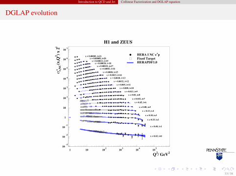
Introduction to QCD and Jet Collinear Factorization and DGLAP equation
DGLAP evolution
H1 and ZEUS
x = 0.00005, i=21x = 0.00008, i=20
x = 0.00013, i=19x = 0.00020, i=18
x = 0.00032, i=17x = 0.0005, i=16
x = 0.0008, i=15x = 0.0013, i=14
x = 0.0020, i=13x = 0.0032, i=12
x = 0.005, i=11x = 0.008, i=10
x = 0.013, i=9x = 0.02, i=8
x = 0.032, i=7x = 0.05, i=6
x = 0.08, i=5x = 0.13, i=4
x = 0.18, i=3
x = 0.25, i=2
x = 0.40, i=1
x = 0.65, i=0
Q2/ GeV2
r,N
C(x
,Q2 ) x
2i
+
HERA I NC e+pFixed TargetHERAPDF1.0
10-3
10-2
10-1
1
10
10 2
10 3
10 4
10 5
10 6
10 7
1 10 10 2 10 3 10 4 10 5
33 / 38
Introduction to QCD and Jet Collinear Factorization and DGLAP equation
DGLAP evolution
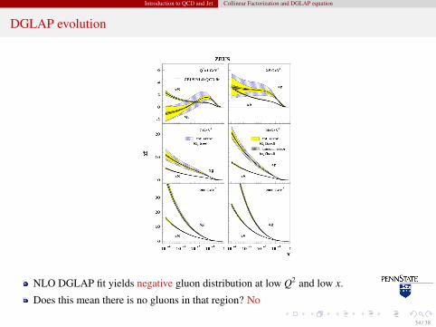
NLO DGLAP fit yields negative gluon distribution at low Q2 and low x.
Does this mean there is no gluons in that region? No
34 / 38
Introduction to QCD and Jet Collinear Factorization and DGLAP equation
Phase diagram in QCD
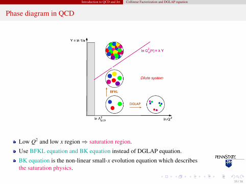
Low Q2 and low x region⇒ saturation region.
Use BFKL equation and BK equation instead of DGLAP equation.
BK equation is the non-linear small-x evolution equation which describesthe saturation physics.
35 / 38
Introduction to QCD and Jet Collinear Factorization and DGLAP equation
Collinear Factorization vs k⊥ Factorization
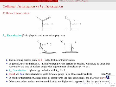
Collinear Factorization
xp+, k⊥ = 0 xp+, k⊥ = 0
k⊥ Factorization(Spin physics and saturation physics)
The incoming partons carry no k⊥ in the Collinear Factorization.In general, there is intrinsic k⊥. It can be negligible for partons in protons, but should be taken intoaccount for the case of nucleus target with large number of nucleons (A→∞).k⊥ Factorization: High energy evolution with k⊥ fixed.Initial and final state interactions yield different gauge links. (Process dependent)In collinear factorization, gauge links all disappear in the light cone gauge, and PDFs are universal.Other approaches, such as nuclear modification and higher twist approach. (See last year’s lecture.)
36 / 38
Introduction to QCD and Jet Transverse Momentum Dependent (TMD or kt ) Factorization
kt dependent parton distributions
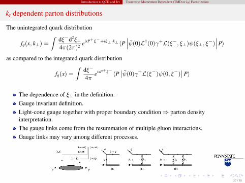
The unintegrated quark distribution
fq(x, k⊥) =
∫dξ−d2ξ⊥4π(2π)2 eixP+ξ−+iξ⊥·k⊥〈P
∣∣∣ψ(0)L†(0)γ+L(ξ−, ξ⊥)ψ(ξ⊥, ξ−)∣∣∣P〉
as compared to the integrated quark distribution
fq(x) =
∫dξ−
4πeixP+ξ−〈P
∣∣ψ(0)γ+L(ξ−)ψ(0, ξ−)∣∣P〉
The dependence of ξ⊥ in the definition.Gauge invariant definition.Light-cone gauge together with proper boundary condition⇒ parton densityinterpretation.The gauge links come from the resummation of multiple gluon interactions.Gauge links may vary among different processes.
37 / 38
Introduction to QCD and Jet Transverse Momentum Dependent (TMD or kt ) Factorization
TMD factorization
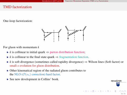
One-loop factorization:
For gluon with momentum k
k is collinear to initial quark⇒ parton distribution function;
k is collinear to the final state quark⇒ fragmentation function.
k is soft divergence (sometimes called rapidity divergence)⇒Wilson lines (Soft factor) orsmall-x evolution for gluon distribution.
Other kinematical region of the radiated gluon contributes tothe NLO (O(αs) correction) hard factor.
See new development in Collins’ book.
38 / 38