Robotics

Reinforcement Learning in Robotics

Marc ToussaintUniversity of Stuttgart

Winter 2014/15

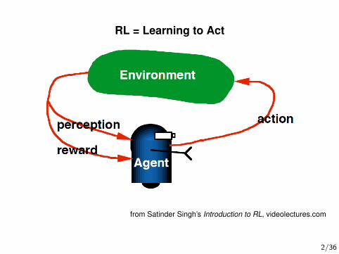
RL = Learning to Act

from Satinder Singh’s Introduction to RL, videolectures.com

2/36

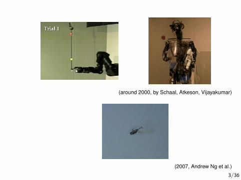
(around 2000, by Schaal, Atkeson, Vijayakumar)

(2007, Andrew Ng et al.)

3/36

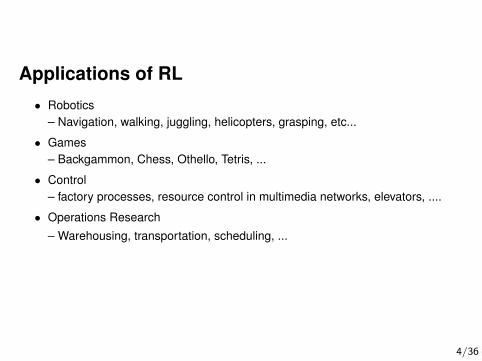
Applications of RL

• Robotics– Navigation, walking, juggling, helicopters, grasping, etc...

• Games– Backgammon, Chess, Othello, Tetris, ...

• Control– factory processes, resource control in multimedia networks, elevators, ....

• Operations Research

– Warehousing, transportation, scheduling, ...

4/36

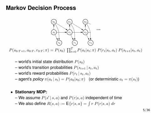
Markov Decision Process

a0

s0

r0

a1

s1

r1

a2

s2

r2

P (s0:T+1, a0:T , r0:T ;π) = P (s0)∏Tt=0 P (at|st;π) P (rt|st, at) P (st+1|st, at)

– world’s initial state distribution P (s0)

– world’s transition probabilities P (st+1 | st, at)– world’s reward probabilities P (rt | st, at)– agent’s policy π(at | st) = P (a0|s0;π) (or deterministic at = π(st))

• Stationary MDP:– We assume P (s′ | s, a) and P (r|s, a) independent of time– We also define R(s, a) := E{r|s, a} =

∫r P (r|s, a) dr

5/36

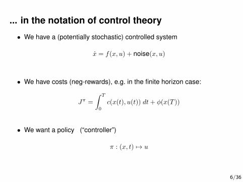
... in the notation of control theory

• We have a (potentially stochastic) controlled system

x = f(x, u) + noise(x, u)

• We have costs (neg-rewards), e.g. in the finite horizon case:

Jπ =

∫ T

0

c(x(t), u(t)) dt+ φ(x(T ))

• We want a policy (“controller”)

π : (x, t) 7→ u

6/36

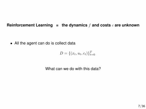
Reinforcement Learning = the dynamics f and costs c are unknown

• All the agent can do is collect data

D = {(xt, ut, ct)}Tt=0

What can we do with this data?

7/36

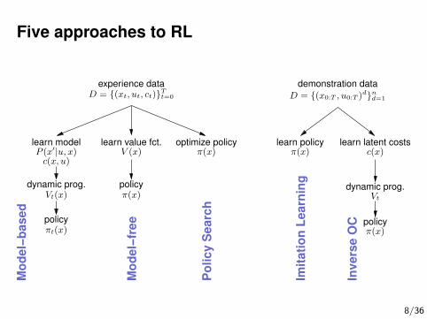
Five approaches to RLM

od

el−

ba

se

d

Inv

ers

e O

C

Imit

ati

on

Le

arn

ing

Po

lic

y S

ea

rch

Mo

de

l−fr

eelearn value fct.

V (x)

policyπ(x)

optimize policy learn latent costsc(x)

dynamic prog.

π(x)policy

learn policyπ(x)

policy

learn model

πt(x)

P (x′|u, x)c(x, u)

dynamic prog.Vt(x) Vt

π(x)

demonstration dataexperience dataD = {(xt, ut, ct)}Tt=0 D = {(x0:T , u0:T )

d}nd=1

8/36

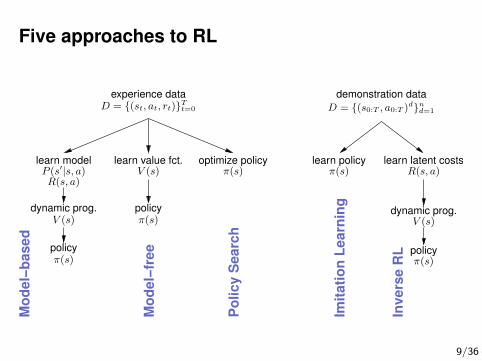
Five approaches to RL

Po

lic

y S

ea

rch

Inv

ers

e R

L

Imit

ati

on

Le

arn

ing

Mo

de

l−fr

ee

Mo

de

l−b

as

ed

learn value fct.V (s)

policyπ(s)

optimize policy learn latent costsR(s, a)

dynamic prog.

π(s)policy

learn policyπ(s)

policy

learn model

π(s)

P (s′|s, a)R(s, a)

dynamic prog.V (s) V (s)

π(s)

demonstration dataexperience dataD = {(s0:T , a0:T )d}nd=1

D = {(st, at, rt)}Tt=0

9/36

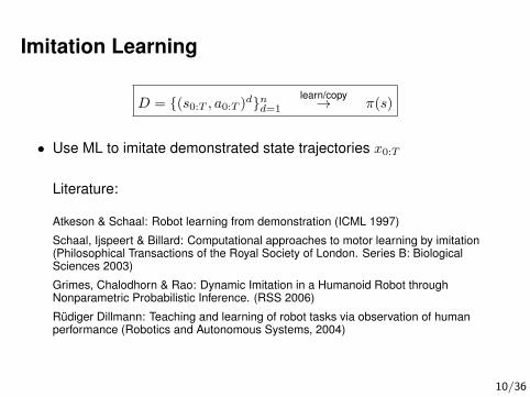
Imitation Learning

D = {(s0:T , a0:T )d}nd=1

learn/copy→ π(s)

• Use ML to imitate demonstrated state trajectories x0:T

Literature:

Atkeson & Schaal: Robot learning from demonstration (ICML 1997)

Schaal, Ijspeert & Billard: Computational approaches to motor learning by imitation(Philosophical Transactions of the Royal Society of London. Series B: BiologicalSciences 2003)

Grimes, Chalodhorn & Rao: Dynamic Imitation in a Humanoid Robot throughNonparametric Probabilistic Inference. (RSS 2006)

Rudiger Dillmann: Teaching and learning of robot tasks via observation of humanperformance (Robotics and Autonomous Systems, 2004)

10/36

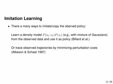
Imitation Learning

• There a many ways to imitate/copy the oberved policy:

Learn a density model P (at | st)P (st) (e.g., with mixture of Gaussians)from the observed data and use it as policy (Billard et al.)

Or trace observed trajectories by minimizing perturbation costs(Atkeson & Schaal 1997)

11/36

Imitation Learning

Atkeson & Schaal12/36

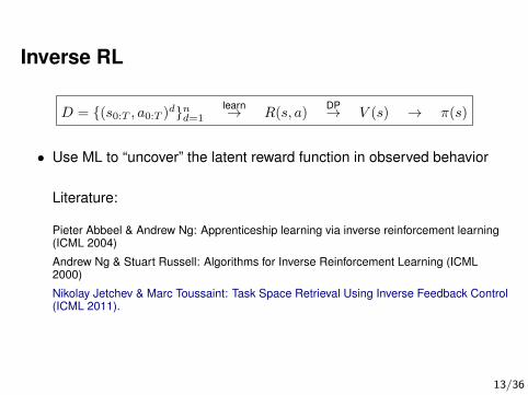
Inverse RL

D = {(s0:T , a0:T )d}nd=1learn→ R(s, a)

DP→ V (s) → π(s)

• Use ML to “uncover” the latent reward function in observed behavior

Literature:

Pieter Abbeel & Andrew Ng: Apprenticeship learning via inverse reinforcement learning(ICML 2004)

Andrew Ng & Stuart Russell: Algorithms for Inverse Reinforcement Learning (ICML2000)

Nikolay Jetchev & Marc Toussaint: Task Space Retrieval Using Inverse Feedback Control(ICML 2011).

13/36

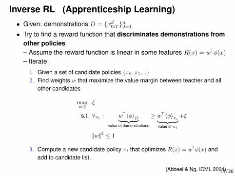
Inverse RL (Apprenticeship Learning)• Given: demonstrations D = {xd0:T }nd=1

• Try to find a reward function that discriminates demonstrations fromother policies– Assume the reward function is linear in some features R(x) = w>φ(x)

– Iterate:

1. Given a set of candidate policies {π0, π1, ..}2. Find weights w that maximize the value margin between teacher and all

other candidates

maxw,ξ

ξ

s.t. ∀πi : w>〈φ〉D︸ ︷︷ ︸value of demonstrations

≥ w>〈φ〉πi︸ ︷︷ ︸value of πi

+ξ

||w||2 ≤ 1

3. Compute a new candidate policy πi that optimizes R(x) = w>φ(x) andadd to candidate list.

(Abbeel & Ng, ICML 2004)14/36

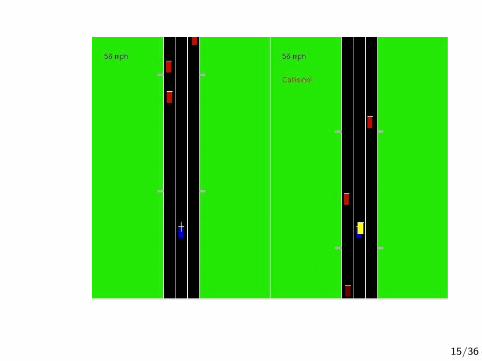
15/36

Policy Search with Policy Gradients

16/36

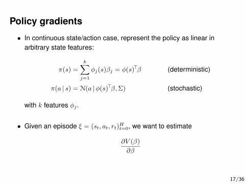
Policy gradients

• In continuous state/action case, represent the policy as linear inarbitrary state features:

π(s) =

k∑j=1

φj(s)βj = φ(s)>β (deterministic)

π(a | s) = N(a |φ(s)>β,Σ) (stochastic)

with k features φj .

• Given an episode ξ = (st, at, rt)Ht=0, we want to estimate

∂V (β)

∂β

17/36

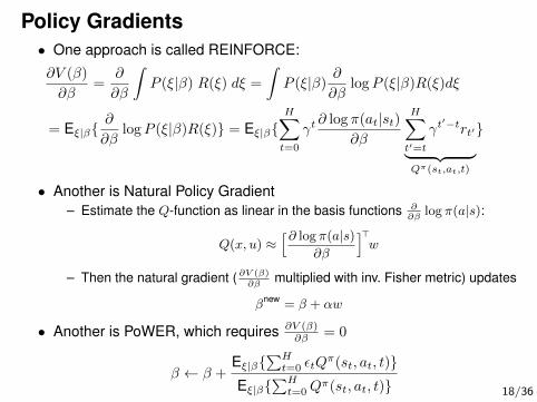
Policy Gradients• One approach is called REINFORCE:

∂V (β)

∂β=

∂

∂β

∫P (ξ|β) R(ξ) dξ =

∫P (ξ|β)

∂

∂βlogP (ξ|β)R(ξ)dξ

= Eξ|β{∂

∂βlogP (ξ|β)R(ξ)} = Eξ|β{

H∑t=0

γt∂ log π(at|st)

∂β

H∑t′=t

γt′−trt′︸ ︷︷ ︸

Qπ(st,at,t)

}

• Another is Natural Policy Gradient– Estimate the Q-function as linear in the basis functions ∂

∂βlog π(a|s):

Q(x, u) ≈[∂ log π(a|s)

∂β

]>w

– Then the natural gradient ( ∂V (β)∂β

multiplied with inv. Fisher metric) updates

βnew = β + αw

• Another is PoWER, which requires ∂V (β)∂β = 0

β ← β +Eξ|β{

∑Ht=0 εtQ

π(st, at, t)}Eξ|β{

∑Ht=0Q

π(st, at, t)} 18/36

Kober & Peters: Policy Search for Motor Primitives in Robotics, NIPS 2008.

(serious reward shaping!)

19/36

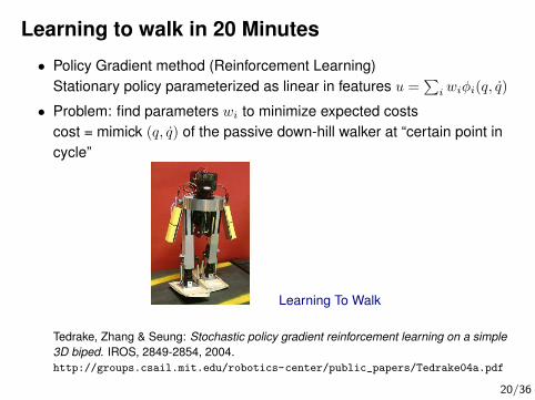
Learning to walk in 20 Minutes

• Policy Gradient method (Reinforcement Learning)Stationary policy parameterized as linear in features u =

∑i wiφi(q, q)

• Problem: find parameters wi to minimize expected costscost = mimick (q, q) of the passive down-hill walker at “certain point incycle”

Learning To Walk

Tedrake, Zhang & Seung: Stochastic policy gradient reinforcement learning on a simple3D biped. IROS, 2849-2854, 2004.http://groups.csail.mit.edu/robotics-center/public_papers/Tedrake04a.pdf

20/36

Policy Gradients – referencesPeters & Schaal (2008): Reinforcement learning of motor skills with policy gradients,Neural Networks.

Kober & Peters: Policy Search for Motor Primitives in Robotics, NIPS 2008.

Vlassis, Toussaint (2009): Learning Model-free Robot Control by a Monte Carlo EMAlgorithm. Autonomous Robots 27, 123-130.

Rawlik, Toussaint, Vijayakumar(2012): On Stochastic Optimal Control andReinforcement Learning by Approximate Inference. RSS 2012. (ψ-learning)

• These methods are sometimes called white-box optimization:They optimize the policy parameters β for the total reward R =

∑γtrt

while tying to exploit knowledge of how the process is actuallyparameterized

21/36

Black-Box Optimization

22/36

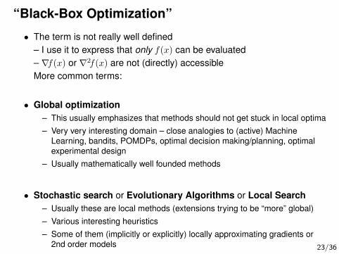
“Black-Box Optimization”

• The term is not really well defined– I use it to express that only f(x) can be evaluated– ∇f(x) or ∇2f(x) are not (directly) accessibleMore common terms:

• Global optimization– This usually emphasizes that methods should not get stuck in local optima– Very very interesting domain – close analogies to (active) Machine

Learning, bandits, POMDPs, optimal decision making/planning, optimalexperimental design

– Usually mathematically well founded methods

• Stochastic search or Evolutionary Algorithms or Local Search– Usually these are local methods (extensions trying to be “more” global)– Various interesting heuristics– Some of them (implicitly or explicitly) locally approximating gradients or

2nd order models 23/36

Black-Box Optimization

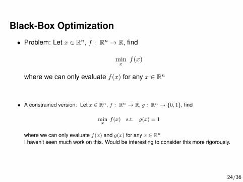
• Problem: Let x ∈ Rn, f : Rn → R, find

minx

f(x)

where we can only evaluate f(x) for any x ∈ Rn

• A constrained version: Let x ∈ Rn, f : Rn → R, g : Rn → {0, 1}, find

minx

f(x) s.t. g(x) = 1

where we can only evaluate f(x) and g(x) for any x ∈ RnI haven’t seen much work on this. Would be interesting to consider this more rigorously.

24/36

A zoo of approaches

• People with many different backgrounds drawn into thisRanging from heuristics and Evolutionary Algorithms to heavy mathematics

– Evolutionary Algorithms, esp. Evolution Strategies, Covariance MatrixAdaptation, Estimation of Distribution Algorithms

– Simulated Annealing, Hill Climing, Downhill Simplex– local modelling (gradient/Hessian), global modelling

25/36

Optimizing and Learning

• Black-Box optimization is strongly related to learning:

• When we have local a gradient or Hessian, we can take that localinformation and run – no need to keep track of the history or learn(exception: BFGS)

• In the black-box case we have no local information directly accessible→ one needs to account for the history in some way or another to havean idea where to continue search

• “Accounting for the history” very often means learning: Learning a localor global model of f itself, learning which steps have been successfulrecently (gradient estimation), or which step directions, or otherheuristics

26/36

Stochastic Search

27/36

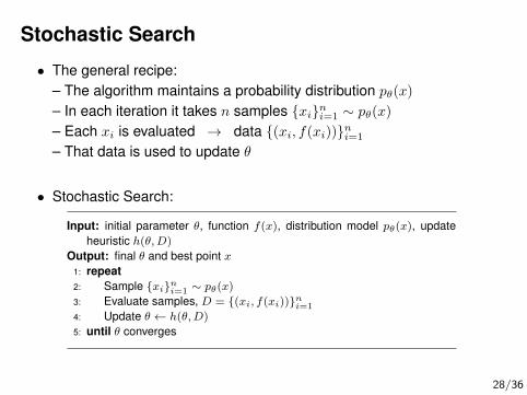
Stochastic Search

• The general recipe:– The algorithm maintains a probability distribution pθ(x)

– In each iteration it takes n samples {xi}ni=1 ∼ pθ(x)

– Each xi is evaluated → data {(xi, f(xi))}ni=1

– That data is used to update θ

• Stochastic Search:

Input: initial parameter θ, function f(x), distribution model pθ(x), updateheuristic h(θ,D)

Output: final θ and best point x1: repeat2: Sample {xi}ni=1 ∼ pθ(x)3: Evaluate samples, D = {(xi, f(xi))}ni=1

4: Update θ ← h(θ,D)

5: until θ converges

28/36

Stochastic Search

• The parameter θ is the only “knowledge/information” that is beingpropagated between iterationsθ encodes what has been learned from the historyθ defines where to search in the future

• Evolutionary Algorithms: θ is a parent populationEvolution Strategies: θ defines a Gaussian with mean & varianceEstimation of Distribution Algorithms: θ are parameters of somedistribution model, e.g. Bayesian NetworkSimulated Annealing: θ is the “current point” and a temperature

29/36

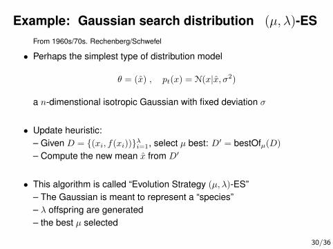
Example: Gaussian search distribution (µ, λ)-ESFrom 1960s/70s. Rechenberg/Schwefel

• Perhaps the simplest type of distribution model

θ = (x) , pt(x) = N(x|x, σ2)

a n-dimenstional isotropic Gaussian with fixed deviation σ

• Update heuristic:– Given D = {(xi, f(xi))}λi=1, select µ best: D′ = bestOfµ(D)

– Compute the new mean x from D′

• This algorithm is called “Evolution Strategy (µ, λ)-ES”– The Gaussian is meant to represent a “species”– λ offspring are generated– the best µ selected

30/36

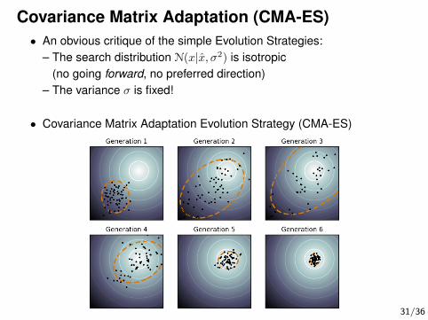
Covariance Matrix Adaptation (CMA-ES)• An obvious critique of the simple Evolution Strategies:

– The search distribution N(x|x, σ2) is isotropic(no going forward, no preferred direction)

– The variance σ is fixed!

• Covariance Matrix Adaptation Evolution Strategy (CMA-ES)

31/36

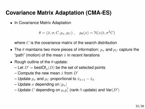
Covariance Matrix Adaptation (CMA-ES)

• In Covariance Matrix Adaptation

θ = (x, σ, C, pσ, pC) , pθ(x) = N(x|x, σ2C)

where C is the covariance matrix of the search distribution

• The θ maintains two more pieces of information: pσ and pC capture the“path” (motion) of the mean x in recent iterations

• Rough outline of the θ-update:– Let D′ = bestOfµ(D) be the set of selected points– Compute the new mean x from D′

– Update pσ and pC proportional to xk+1 − xk– Update σ depending on |pσ|– Update C depending on pcp>c (rank-1-update) and Var(D′)

32/36

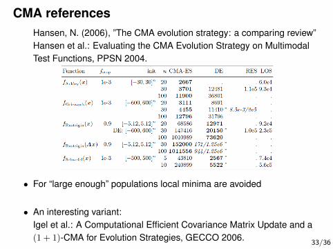
CMA referencesHansen, N. (2006), ”The CMA evolution strategy: a comparing review”Hansen et al.: Evaluating the CMA Evolution Strategy on MultimodalTest Functions, PPSN 2004.

• For “large enough” populations local minima are avoided

• An interesting variant:Igel et al.: A Computational Efficient Covariance Matrix Update and a(1 + 1)-CMA for Evolution Strategies, GECCO 2006.

33/36

CMA conclusions

• It is a good starting point for an off-the-shelf black-box algorithm

• It includes components like estimating the local gradient (pσ, pC), thelocal “Hessian” (Var(D′)), smoothing out local minima (largepopulations)

34/36

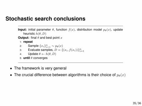
Stochastic search conclusions

Input: initial parameter θ, function f(x), distribution model pθ(x), updateheuristic h(θ,D)

Output: final θ and best point x1: repeat2: Sample {xi}ni=1 ∼ pθ(x)3: Evaluate samples, D = {(xi, f(xi))}ni=1

4: Update θ ← h(θ,D)

5: until θ converges

• The framework is very general

• The crucial difference between algorithms is their choice of pθ(x)

35/36

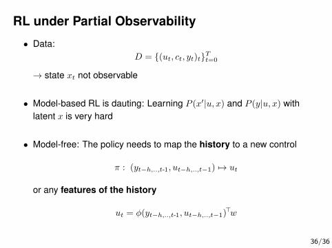
RL under Partial Observability

• Data:D = {(ut, ct, yt)t}Tt=0

→ state xt not observable

• Model-based RL is dauting: Learning P (x′|u, x) and P (y|u, x) withlatent x is very hard

• Model-free: The policy needs to map the history to a new control

π : (yt−h,..,t-1, ut−h,..,t−1) 7→ ut

or any features of the history

ut = φ(yt−h,..,t-1, ut−h,..,t−1)>w

36/36