Embed Size (px)
Citation preview

Introduction to Mobile Robotics
SLAM:
Simultaneous Localizationand Mapping

The SLAM Problem
SLAM is the process by which a robot builds a map of the environment and, at the same time, uses this map to compute its location
• Localization: inferring location given a map
• Mapping: inferring a map given a location
• SLAM: learning a map and locating the robot simultaneously
2
The SLAM Problem
• SLAM is a chicken-or-egg problem:
A map is needed for localizing a robot
A good pose estimate is needed to build a map
•
hus, SLAM is regarded as a hard problem in
robotics 3

4
• SLAM is considered one of the most
fundamental problems for robots to become
truly autonomous.
• A variety of different approaches to address the
SLAM problem have been presented
• Probabilistic methods rule!
• History of SLAM dates back to the mid-eighties
(the stone-age of robotics)
The SLAM Problem

5
Given:
• The robot’s controls
• Relative observations
Wanted:
• Map of features
• Path of the robot
The SLAM Problem

The SLAM Problem
6
• Absoluterobot pose
• Absolutelandmark positions
• But only relative measurements of landmarks

7
Mapping with Raw Odometry
Video..

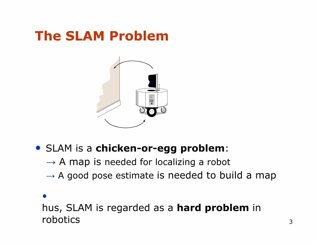
SLAM Applications
SLAM is central to a range of indoor, outdoor, in-air and underwater applications for both manned and autonomous vehicles.
Examples:
•At home: vacuum cleaner, lawn mower
•Air: surveillance with unmanned air vehicles
•Underwater: reef monitoring
•Underground: exploration of abandoned mines
•Space: terrain mapping for localization
8
9
SLAM Applications
Indoors
Space
Undersea
Underground
10
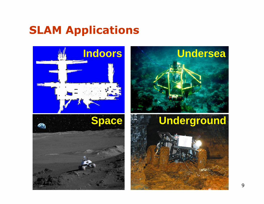
Map Representations
Examples:
Subway map, city map, landmark-based map
Maps are topological and/or metric
models of the environment

11
Map Representations
• Grid maps or scans, 2d, 3d
[Lu & Milios, 97; Gutmann, 98: Thrun 98; Burgard, 99; Konolige & Gutmann, 00; Thrun, 00; Arras,
99; Haehnel, 01;…]
• Landmark-based
[Leonard et al., 98; Castelanos et al., 99: Dissanayake et al., 2001; Montemerlo et al., 2002;…

12
Why is SLAM a hard problem?
1. Robot path and map are both unknown
2. Errors in map and pose estimates correlated

13
Why is SLAM a hard problem?
• In the real world, the mapping between observations and landmarks is unknown (origin uncertainty of measurements)
• Data Association: picking wrong data associations can have catastrophic consequences (divergence)
Robot poseuncertainty

14
SLAM: Simultaneous Localization And Mapping
• Full SLAM:
• Online SLAM:
Integrations (marginalization) typically done recursively, one at a time
p(x0:t,m |z1:t ,u1:t )
p(x t,m |z1:t ,u1:t ) = K p(x1:t ,m |z1:t,u1:t ) dx1∫∫∫ dx2...dx t−1
Estimates most recent pose and map!
Estimates entire path and map!

15
Graphical Model of Full SLAM
),|,( :1:1:1 ttt uzmxp

16
Graphical Model of Online SLAM
121:1:1:1:1:1 ...),|,(),|,( −∫ ∫ ∫= ttttttt dxdxdxuzmxpuzmxp Κ

17
Graphical Model: Models
Motion model
Observation model

18
Remember? KF Algorithm
1. Algorithm Kalman_filter(µt-1, Σt-1, ut, zt):
2. Prediction:
3.
4.
5. Correction:
6.
7.
8.
9. Return µt, Σt
ttttt uBA += −1µµt
Ttttt RAA +Σ=Σ −1
1)( −+ΣΣ= tTttt
Tttt QCCCK
)( tttttt CzK µµµ −+=tttt CKI Σ−=Σ )(

EKF SLAM: State representation
• Localization
3x1 pose vector
3x3 cov. matrix
• SLAM
Landmarks are simply added to the state.
Growing state vector and covariance matrix!
19

Bel(xt,mt) =
x
y
θl1l2M
lN
,
σx2 σxy σxθ σxl1
σxl2L σxlN
σxy σy2 σyθ σyl1
σyl2L σylN
σxθ σyθ σθ2 σθl1
σθl2L σθlN
σxl1σyl1
σθl1σl1
2 σl1l2L σl1lN
σxl2σyl2
σθl2σl1l2
σl2
2 L σl2lN
M M M M M O M
σxlNσylN
σθlNσl1lN
σl2lNL σlN
2
• Map with n landmarks: (3+2n)-dimensional Gaussian
• Can handle hundreds of dimensions
20
EKF SLAM: State representation

• State Prediction
EKF SLAM: Building The Map
21
Odometry:
(skipping time index k)
Robot-landmark cross-covariance prediction:

EKF SLAM: Building The Map
• Measurement Prediction
22
Global-to-local frame transform h

• Observation
EKF SLAM: Building The Map
23
(x,y)-point landmarks

Associates predicted measurementswith observation
• Data Association
EKF SLAM: Building The Map
24
? (Gating)

EKF SLAM: Building The Map
• Filter Update
25
The usual Kalman filter expressions

• Integrating New Landmarks
EKF SLAM: Building The Map
26
State augmented by
landmark-to-landmark cross-covariance:

27
EKF SLAM
Map Correlation matrix

28
EKF SLAM
Map Correlation matrix

29
EKF SLAM
Map Correlation matrix
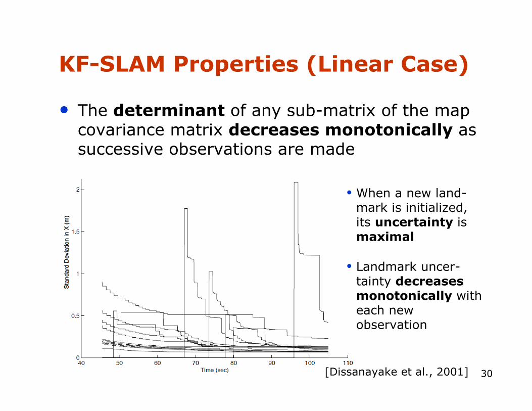
• The determinant of any sub-matrix of the map covariance matrix decreases monotonically as successive observations are made
30
KF-SLAM Properties (Linear Case)
[Dissanayake et al., 2001]
• When a new land-mark is initialized,its uncertainty is maximal
• Landmark uncer-tainty decreases monotonically with each new observation

• In the limit, the landmark estimates become fully correlated
31
KF-SLAM Properties (Linear Case)
[Dissanayake et al., 2001]

• In the limit, the covariance associated with any single landmark location estimate is determined only by the initial covariance in the vehicle location estimate.
32
KF-SLAM Properties (Linear Case)
[Dissanayake et al., 2001]

33
Victoria Park Data Set
[courtesy by E. Nebot]

34
Victoria Park Data Set Vehicle
[courtesy by E. Nebot]

35
Data Acquisition
[courtesy by E. Nebot]

36
Estimated Trajectory
[courtesy by E. Nebot]

37
EKF SLAM Application
[courtesy by J. Leonard]

38
EKF SLAM Application
odometry estimated trajectory
[courtesy by John Leonard]

39
SLAM Techniques for Generating Consistent Maps
• EKF SLAM
• FastSLAM (PF)
• Network-Based SLAM
• Hybrid Approaches(combination of NW+PF, NW+EKF)
• Topological SLAM(mainly place recognition)
• Scan Matching / Visual Odometry(only locally consistent maps)
40
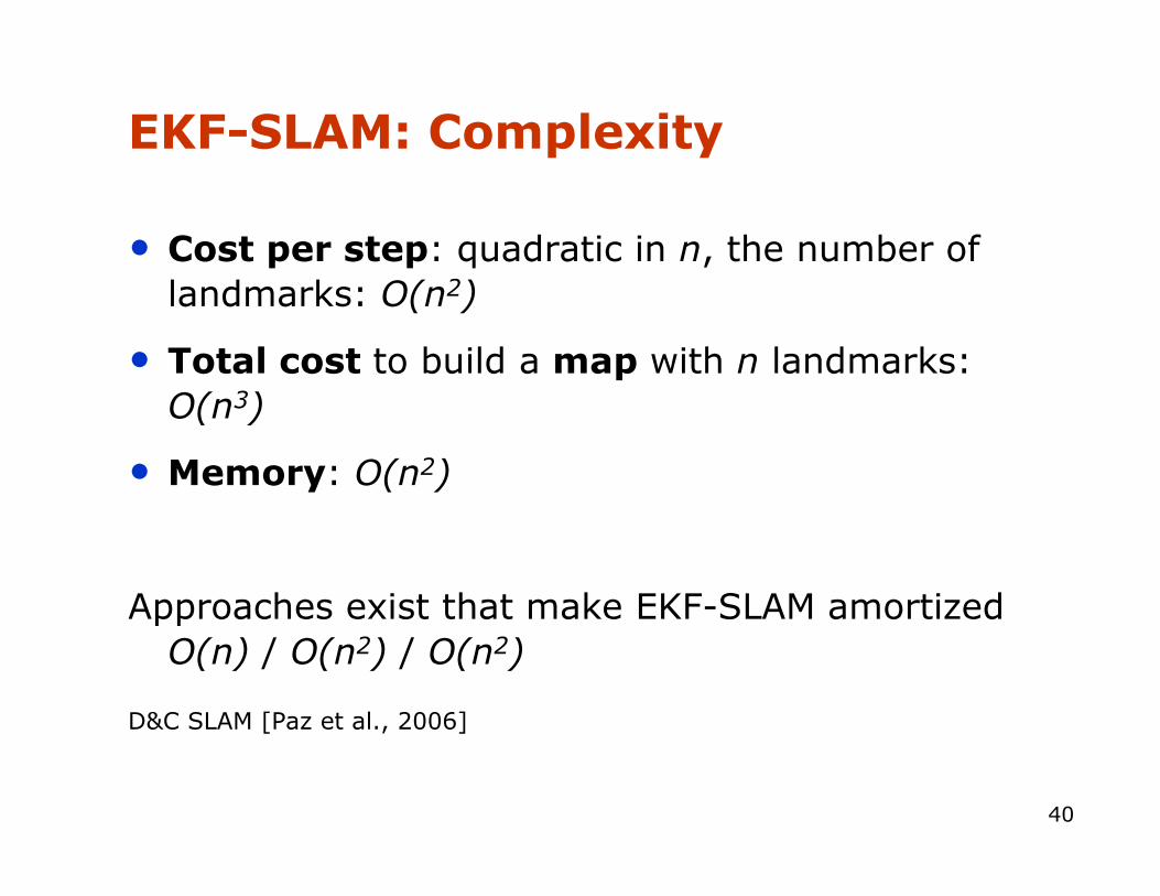
EKF-SLAM: Complexity
• Cost per step: quadratic in n, the number of
landmarks: O(n2)
• Total cost to build a map with n landmarks:
O(n3)
• Memory: O(n2)
Approaches exist that make EKF-SLAM amortized
O(n) / O(n2) / O(n2)
D&C SLAM [Paz et al., 2006]

41
EKF-SLAM: Summary
• Convergence for linear case!
• Can diverge if nonlinearities are large.And reality is nonlinear...
• Has been applied successfully in large-scale environments
• Approximations reduce the computational complexity

42
Data Association for SLAM
Interpretation tree

43
Data Association for SLAM
Env. Dyn.

44
Data Association for SLAM
Geometric Constraints
Location independent constraints
Unary constraint:intrinsic property of featuree.g. type, color, size
Binary constraint:relative measure between featurese.g. relative position, angle
Location dependent constraints
Rigidity constraint:"is the feature where I expect it givenmy position?"
Visibility constraint:"is the feature visible from my position?"
Extension constraint:"do the features overlap at my position?"
All decisions on a significance level α

45
Data Association for SLAM
Interpretation Tree[Grimson 1987], [Drumheller 1987],
[Castellanos 1996], [Lim 2000]
Algorithm
• backtracking
• depth-first
• recursive
• uses geometric constraints
• exponential complexity
• absence of feature: no info.
• presence of feature: info. perhaps

46
Data Association for SLAM
Pygmalion
a = 0.95 , p = 2

47
Data Association for SLAM
a = 0.95 , p = 3
Pygmalion

48
Data Association for SLAM
a = 0.95 , p = 4a = 0.95 , p = 5
texe: 633 msPowerPC at 300
MHz
Pygmalion

49
• Local submaps [Leonard et al.99, Bosse et al. 02, Newman et al. 03]
• Sparse links (correlations) [Lu & Milios 97, Guivant & Nebot 01]
• Sparse extended information filters [Frese et al. 01, Thrun et al. 02]
• Thin junction tree filters [Paskin 03]
• Rao-Blackwellisation (FastSLAM) [Murphy 99, Montemerlo et al. 02, Eliazar et al. 03, Haehnel et al. 03]
Approximations for SLAM