Embed Size (px)
Citation preview
N. V. AZBELEV V. P. MAKSIMOV
L. F. RAKHMATULLINA
INTRODUCTION TO THE THEORY OF
FUNCTIONAL DIFFERENTIAL
EQUATIONSMETHODS AND APPLICATIONS
Introduction to the Theory ofFunctional Differential Equations:Methods and Applications


Contemporary Mathematics and Its Applications, Volume 3
Introduction to the Theory ofFunctional Differential Equations:Methods and ApplicationsN. V. Azbelev, V. P. Maksimov, and L. F. Rakhmatullina
Hindawi Publishing Corporationhttp://www.hindawi.com
Contemporary Mathematics and Its ApplicationsSeries Editors: Ravi P. Agarwal and Donal O’Regan
Hindawi Publishing Corporation410 Park Avenue, 15th Floor, #287 pmb, New York, NY 10022, USANasr City Free Zone, Cairo 11816, EgyptFax: +1-866-HINDAWI (USA Toll-Free)
© 2007 Hindawi Publishing Corporation
All rights reserved. No part of the material protected by this copyright notice may be reproduced orutilized in any form or by any means, electronic or mechanical, including photocopying, recording,or any information storage and retrieval system, without written permission from the publisher.
ISBN 977-5945-49-6
Contents
Preface vii
1. Linear abstract functional differential equation 11.1. Preliminary knowledge from the theory of linear equations
in Banach spaces 11.2. Linear equation and linear boundary value problem 61.3. The Green operator 121.4. Problems lacking the everywhere and unique solvability 201.5. Continuous dependence on parameters 29
2. Equations in traditional spaces 412.1. Introduction 412.2. Equations in the space of absolutely continuous functions 422.3. Equations of the nth order 592.4. Equations in spaces of functions defined on the semiaxis 762.5. Equations with generalized Volterra operators 90
3. Equations in finite-dimensional extensions of traditional spaces 993.1. Introduction 993.2. Equations in the space of piecewise absolutely
continuous functions 1003.3. Equations of the nth order with impulse effect 1083.4. Multipoint boundary value problem for the Poisson equation 115
4. Singular equations 1214.1. Introduction 1214.2. The equation (t − a)(b− t)x(t)− (Tx)(t) = f (t) 1224.3. Inner singularities 1374.4. The chemical reactor’s equation 142
5. Minimization of square functionals 1495.1. Introduction 1495.2. The criterion for the existence of the minimum of
the square functional 1495.3. The tests of the existence of the minimum of the functional 157
6. Constructive study of linear problems (using computer algebra inthe study of linear problems) 1736.1. Introduction 173
vi Contents
6.2. General theorem on the solvability of the boundaryvalue problem 174
6.3. BVP in the space of absolutely continuous functions 1776.4. BVP in the space of piecewise absolutely continuous functions 1916.5. Boundary value problem for a singular equation 1936.6. The Cauchy matrix and a posteriori error bounds 1996.7. Other applications of the constructive approach 203
7. Nonlinear equations 2137.1. Introduction 2137.2. Equations with monotone operators 2147.3. Reducibility of equations 2247.4. A priori inequalities 2367.5. Nonlinear boundary value problems 2477.6. Sufficient conditions for minimum of functionals 2517.7. Reducible stochastic functional differential equations 264
8. Appendices 281A. On the spectral radius estimate of a linear operator 281B. A compactness condition for a linear integral operator
in the space of summable functions 284C. The composition operator 285D. Vallee-Poussin-like theorem 296
Bibliography 303
Index 313
Preface
The aim of this book is to develop a unified approach to a wide class of equations.Previously, these equations were studied without any connection. We demonstratehow this general theory can be applied to specific classes of functional differentialequations.
The equation
x = Fx, (1)
with an operator F defined on a set of absolutely continuous functions, is calledthe functional differential equation. Thus (1) is a far-reaching generalization of thedifferential equation
x(t) = f(t, x(t)
). (2)
It covers also the integrodifferential equation
x(t) =∫ b
aK(t, s, x(s)
)ds, (3)
the “delay differential equation”
x(t) = f(t, x[h(t)
]), t ∈ [a, b], h(t) ≤ t,
x(ξ) = ϕ(ξ) if ξ < a,(4)
the “equation with distributed deviation of the argument”
x(t) = f(t,∫ b
ax(s)dsR(t, s)
), (5)
and so on.Some distinctive properties of (2) used in investigations are defined by the
specific character of the so-called “local operator.” An operator Φ : X → Y, whereX and Y are functional spaces, is called local (see Shragin [209], Ponosov [176])if the values of y(t) = (Φx)(t) in any neighborhood of t = t0 depend only on thevalues of x(t) in the same neighborhood.
viii Preface
It is relevant to note that most hypotheses of classical physics assume that therate (d/dt)x of change of the state x of the process at the time t0 depends only onthe state of the process at the same time. Thus the mathematical description ofsuch a process takes the form (2). The operator d/dt of differentiation as well asthe Nemytskii operator
(Nx)(t)def= f
(t, x(t)
)(6)
are the representatives of the class of local operators. The property of being localof
(Φx)(t)def= x(t)− f
(t, x(t)
)(7)
does not allow using equation (2) in description of processes where there is no wayto ignore the past or future states of process. Thus some problems are in need of ageneralization of (2), consisting in replacement of the local Nemytskii operator Nby a more general F.
Here another principal generalization of (2) should be reminded of, where thefinite-dimensional space Rn of the values of solutions x is replaced by an arbitraryBanach space B. On the base of such generalization, there has arisen recently anew chapter of analysis: “the theory of ordinary differential equations in Banachspaces.” This theory considers certain partial differential equations as the equation(2), where the values of x(t) belong to an appropriate Banach space. But, underthis generalization, the operator (Φx)(t) = x(t) − f (t, x(t)) still remains to belocal. Theory of equation (1) is thoroughly treated by Azbelev et al. in [32]. Thefollowing fact is of fundamental importance: the space D of absolutely continuousfunctions x : [a, b] → Rn is isomorphic to the direct product of the space L ofsummable functions z : [a, b] → Rn and the finite-dimensional space Rn. Recallthat the absolutely continuous function x is defined by
x(t) =∫ t
az(s)ds + α, (8)
where z ∈ L, α ∈ Rn. The space D is Banach under the norm
‖x‖D = ‖x‖L +∥∥x(a)
∥∥
Rn . (9)
In the theory of (1), the specific character of the Lebesgue space L is used only inconnection with the representation of operators in L and some of their properties.Only the fact that L is a Banach space is used, and most of the fundamentals ofthe general theory of (1) keep after replacement of the Lebesgue space L by anarbitrary Banach space B. Thus there arises a new theory of the equations in thespace D isomorphic to the direct product B×Rn (D � B×Rn). The generalizationconsists here in replacement of the Lebesgue space L by an arbitrary Banach spaceB and in replacement of local operators by general ones acting from D � B × Rn
Preface ix
into B. The present book is devoted to the theory of such generalization and tosome applications. The central idea of applications of the theory of abstract dif-ferential equation lies in the proper choice of the space D for each new problem.With the general theory, such a choice permits applying standard schemes andtheorems of analysis to the problems which needed previously an individual ap-proach and special constructions. The boundary value problem is the main pointof consideration.
This theory was worked out during a quarter of century by a large group ofmathematicians united by the so-called Perm Seminar. The results of the membersof the seminar were published in journals as well as in the annuals “BoundaryValue Problems” and “Functional Differential Equations” issued in 1976–1992 bythe Perm Polytechnic Institute.
In the book, only the works closely related to the questions under considera-tion are cited.
It is assumed that the reader is acquainted with the foundations of functionalanalysis.
Let us give some remarks on the format. Each chapter is divided into num-bered sections, some of which are divided into numbered subsections. Formulasand results, whether they are theorems, propositions, or lemmas, as well as re-marks, are numbered consecutively within each chapter. For example, the fourthformula (theorem) of Chapter 2 is labeled (2.4) (Theorem 2.4). Formulas, proposi-tions, and remarks of appendicies are numbered within each section. For example,the third formula of Section A is labeled (A.3).
The authors would like to thank the members of the Perm Seminar for theuseful discussion and especially T.A. Osechkina for the excellent typesetting ofthis manuscript. We would also like to acknowledge the support from the RussianFoundation for Basic Research and the PROGNOZ Company, Russia.
N. V. AzbelevV. P. Maksimov
L. F. Rakhmatullina

1Linear abstract functionaldifferential equation
1.1. Preliminary knowledge from the theory of linear equationsin Banach spaces
The main assertions of the theory of linear abstract functional differential equa-tions are based on the theorems about linear equations in Banach spaces. We givehere without proofs certain results of the book of Krein [122] which we will needbelow. We formulate some of these assertions not in the most general form, but inthe form satisfying our aims. The enumeration of the theorems in brackets meansthat the assertion either coincides with the corresponding result of the book ofKrein [122] or is only an extraction from this result.
We will use the following notations.X, Y, Z are Banach spaces; A, B are linear operators; D(A) is a domain of
definition of A; R(A) is a range of values of A; and A∗ is an operator adjoint to A.The set of solutions of the equation Ax = 0 is said to be a null space or a kernel ofA and is denoted by kerA. The dimension of a linear set M is denoted by dimM.
Let A be acting from X into Y. The equation
Ax = y (1.1)
(the operator A) is said to be normally solvable if the set R(A) is closed; (1.1) is saidto be a Noether equation if it is a normally solvable one, and, besides, dim kerA <∞and dim kerA∗ <∞. The number indA = dim kerA−dim kerA∗ is said to be theindex of the operator A (1.1). If A is a Noether operator and indA = 0, equation(1.1) (the operator A) is said to be a Fredholm one. The equation A∗ϕ = g is saidto be an equation adjoint to (1.1).
Theorem 1.1 (Krein [122, Theorem 3.2]). An operator A is normally solvable if andonly if (1.1) is solvable for such and only such right-hand side y which is orthogonalto all solutions of the homogenous adjoint equation A∗ϕ = 0.
Theorem 1.2 (Krein [122, Theorem 16.4]). The property of being Noether operatoris stable in respect to completely continuous perturbations. By such a perturbation,the index of the operator does not change.
2 Linear abstract functional differential equation
Theorem 1.3 (Krein [122, Theorem 12.2]). Let A be acting from X into Y and letD(B) be dense in Y. If A and B are Noether operators, BA is also a Noether one andind(BA) = indA + indB.
Theorem 1.4 (Krein [122, Theorem 15.1]). Let BA be a Noether operator and letD(B) ⊂ R(A). Then B is a Noether operator.
Theorem 1.5 (Krein [122, Theorem 2.4 and Lemma 8.1]). Let A be defined on Xand acting into Y. A is normally solvable and dim kerA∗ = n if and only if the spaceY is representable in the form of the direct sum Y = R(A)
⊕Mn, where Mn is a
finite-dimensional subspace of the dimension n.
Theorem 1.6 (Krein [122, Theorem 12.2]). Let D(A) ⊂ X, let Mn be an n-dimen-sional subspace of X, and let D(A) ∩Mn = {0}. If A is a Noether operator, then itslinear extension A onD(A)⊕Mn is also a Noether operator. Besides ind A = indA+n.
Theorem 1.7. Let a Noether operatorA be defined on X and acting into Y, letD(B) =Y, and let BA : X → Z be a Noether operator. Then B is also a Noether operator.
Proof. By Theorem 1.4, we are in need only of the proof of the case R(A) �= Y.From Theorem 1.4, we obtain also that the restriction B of B on R(A) is a Noetheroperator.
Let dim kerA∗ = n. Then we have from Theorem 1.5 that
Y = R(A)⊕Mn = D(B)⊕Mn, (1.2)
where dimMn = n.From Theorem 1.6, we see that B is a Noether operator as a linear extension
of B on Y. �A linear operator A acting from a direct product X1 ×X2 into Y is defined by
a pair of operators A1 : X1 → Y and A2 : X2 → Y such that
A{x1, x2
} = A1x1 + A2x2, x1 ∈ X1, x2 ∈ X2, (1.3)
where A1x1 = A{x1, 0} and A2x2 = A{0, x2}. We will denote such an operator byA = {A1,A2}.
A linear operator A acting from X into a direct product Y1 ×Y2 is denoted bya pair of operators A1 : X → Y1 and A2 : X → Y2 so that Ax = {A1x,A2x}, x ∈ X.We will denote such an operator by A = [A1,A2].
The theory of linear abstract functional differential equation is using someoperators defined on a product B × Rn or acting in such a product. We will for-mulate here certain assertions about such operators, preserving as far as possiblethe notation from Azbelev et al. [32, 33].
A linear operator acting from a direct product B×Rn of the Banach spaces Band Rn into a Banach space D is defined by a pair of linear operators Λ : B → D
Preliminary knowledge from the theory of linear equations in Banach spaces 3
and Y : Rn → D in such a way that
{Λ,Y}{z,β} = Λz + Yβ, z ∈ B, β ∈ Rn. (1.4)
A linear operator acting from a space D into a direct product B×Rn is definedby a pair of linear operators δ : D → B and r : D → Rn so that
[δ, r]x = {δx, rx}, x ∈ D. (1.5)
If the norm in the space B×Rn is defined by a corresponding way, for instance,by
∥∥{z,β}∥∥B×Rn = ‖z‖B + |β|, (1.6)
the space B × Rn will be a Banach one (here and in what follows, | · | denotes anorm in Rn).
If the bounded operator {Λ,Y} : B × Rn → D is the inverse to the boundedoperator [δ, r] : D → B×Rn, then
x = Λδx + Yrx, x ∈ D, δ(Λz + Yβ) = z, r(Λz + Yβ) = β, {z,β} ∈ B×Rn.(1.7)
Hence
Λδ + Yr = I , δΛ = I , δY = 0, rΛ = 0, rY = I. (1.8)
We will identify the finite-dimensional operator Y : Rn → D with a vector(y1, . . . , yn), yi ∈ D, such that
Yβ =n∑
i=1
yiβi, β = col
{β1, . . . ,βn
}. (1.9)
We denote the components of the vector functional r by r1, . . . , rn.If l = [l1, . . . , lm] : D → Rm is a linear vector functional, X = (x1, . . . , xn) is a
vector with components xi ∈ D, then lX denotes them×nmatrix, whose columnsare the values of the vector functional l on the components of X : lX = (lix j),i = 1, . . . ,m, j = 1, . . . ,n.
Consider the form of the operators Λ, Y , δ, r for some actual spaces.Let D be the space of absolutely continuous functions x : [a, b] → Rn and let
L be the space of summable z : [a, b] → Rn. The isomorphism between the spaceD and the product B×Rn may be defined, for instance, by
x(t) =∫ t
az(s)ds + β, x ∈ D, {z,β} ∈ L×R
n. (1.10)
4 Linear abstract functional differential equation
In such a case,
(Λz)(t) =∫ t
az(s)ds, Y = E, δx = x, rx = x(a), (1.11)
where E is the identity n× n matrix.In the case of the space Wn of functions x : [a, b] → R1 with absolutely con-
tinuous derivative x(n−1), we obtain similarly that
(Λz)(t) =∫ t
a
(t − s)n−1
(n− 1)!z(s)ds,
Y =(
1, t − a, . . . ,(t − a)n−1
(n− 1)!
),
δx = x(n), rx = {x(a), x(a), . . . , x(n−1)(a)}
,
(1.12)
if the isomorphism between Wn and L×Rn is defined on the base of the represen-tation
x(t) =∫ t
a
(t − s)n−1
(n− 1)!x(n)(s)ds +
n−1∑
k=0
(t − a)k
k!x(k)(a) (1.13)
of the element x ∈ Wn.Denote by DS[a, t1, . . . , tm, b] = DS(m) the space of functions x : [a, b] → Rn
permitting finite discontinuity at the points t1, . . . , tm ∈ (a, b) and being absolutelycontinuous on each [a, t1), [t1, t2), . . . , [tm, b]. The element x ∈ DS(m) may berepresented as
x(t) =∫ t
ax(s)ds + x(a) +
m∑
i=1
χ[ti,b](t)Δx(ti), (1.14)
where Δx(ti) = x(ti)− x(ti − 0), i = 1, . . . ,m, χ[ti ,b] is the characteristic function ofthe interval [ti, b]. Thus the space DS(m) is isomorphic to the product L×Rn(m+1)
and
(Λz)(t) =∫ t
az(s)ds,
Y = (E,E · χ[t1,b], . . . ,E · χ[tm,b]),
δx = x, rx = {x(a),Δx(t1), . . . ,Δx
(tm)}.
(1.15)
Theorem 1.8. A linear bounded operator {Λ,Y} : B × Rn → D has the boundedinverse if and only if the following conditions are satisfied.
(a) The operator Λ : B → D is Noether one and indΛ = −n.(b) dim kerΛ = 0.(c) If λ1, . . . , λn is a basis for kerΛ∗ and λ = {λ1, . . . , λn}, then det λY �= 0.
Preliminary knowledge from the theory of linear equations in Banach spaces 5
Proof
Sufficiency. From (a) and (b), it follows that dim kerΛ∗ = n. By virtue ofTheorem 1.5, D = R(Λ)⊕Mn, where dimMn = n. It follows from (c) that anynontrivial linear combination of elements y1, . . . , yn does not belong to R(Λ),therefore Mn = R(Y). Thus D = R(Λ) ⊕ R(Y) and, consequently, the operator{Λ,Y} has its inverse by virtue of Banach’s theorem.
Necessity. From invertibility of {Λ,Y}, we have D = R(Λ)⊕ R(Y). Consequently,the operator Λ is normally solvable by virtue of Theorem 1.5 and dim kerΛ∗ = n.Besides, dim kerΛ = 0. Therefore indΛ = −n. Assumption det λY = 0 leads tothe conclusion that a nontrivial combination of the elements y1, . . . , yn belongs toR(Λ). �
Theorem 1.9. A linear bounded operator [δ, r] : D → B×Rn has a bounded inverseif and only if the following conditions are satisfied.
(a) The operator δ : D → B is a Noether one, ind δ = n.(b) dim ker δ = n.(c) If x1, . . . , xn is a basis of ker δ and X = (x1, . . . , xn), then det rX �= 0.
Proof
Sufficiency. From (a) and (b), it follows that dim ker δ∗ = 0. Thus R(δ) = B. Eachsolution of the equation δx = z has the form
x =n∑
i=1
cixi + v, (1.16)
where ci = const, i = 1, . . . ,n, v is any solution of this equation. By virtue of (c),the system
δx = z, rx = β (1.17)
has a unique solution for each pair z ∈ B, β ∈ Rn. Therefore, the operator [δ, r]has its bounded inverse.
Necessity. Let [δ, r]−1 = {Λ,Y}. From the equality δΛ = I , by virtue of Theorem1.7, it follows that δ is a Noether operator and, by virtue of Theorem 1.3, ind δ =n. As far as R(δ) = B, we have dim ker δ∗ = 0, and therefore dim ker δ = n. Ifdet rX = 0, then the homogeneous system
δx = 0, rx = 0 (1.18)
has a nontrivial solution. This gives a contradiction to the invertibility of the op-erator [δ, r]. �
6 Linear abstract functional differential equation
1.2. Linear equation and linear boundary value problem
The Cauchy problem
(Lx)(t)def= x(t)− P(t)x(t) = f (t), x(a) = α, t ∈ [a, b], (1.19)
is uniquely solvable for any α ∈ Rn and summable f if the elements of the n × nmatrix P are summable. Thus, the representation of the solution
x(t) = X(t)∫ t
aX−1(s) f (s)ds + X(t)α (1.20)
of the problem (the Cauchy formula), where X is a fundamental matrix such thatX(a) is the identity matrix, is also a representation of the general solution of theequation Lx = f . The Cauchy formula is the base for investigations on variousproblems in the theory of ordinary differential equations. The Cauchy problemfor functional differential equations is not solvable generally speaking, but someboundary value problems may be solvable. Therefore the boundary value problemplays the same role in the theory of functional differential equations as the Cauchyproblem does in the theory of ordinary differential equations.
We will call the equation
Lx = f (1.21)
a linear abstract functional differential equation if L : D → B is a linear operator,D and B are Banach spaces, and the space D is isomorphic to the direct productB×Rn(D � B×Rn).
Let J = {Λ,Y} : B × Rn → D be a linear isomorphism and let J−1 = [δ, r].Everywhere below, the norms in the spaces B×Rn and D are defined by
∥∥{z,β}∥∥B×Rn = ‖z‖B + |β|, ‖x‖D = ‖δx‖B + |rx|. (1.22)
By such a definition of the norms, the isomorphism J is an isometric one. There-fore,
∥∥{Λ,Y}∥∥B×Rn→D = 1,
∥∥[δ, r]
∥∥
D→B×Rn = 1. (1.23)
Since
‖Λz‖D =∥∥{Λ,Y}{z, 0}∥∥D ≤
∥∥{Λ,Y}∥∥∥∥{z, 0}∥∥B×Rn = ‖z‖B, (1.24)
‖Λ‖B→D = 1. Similarly it is stated that ‖Y‖Rn→D = 1. Next, we have
‖δx‖B ≤ ‖x‖D, (1.25)
Linear equation and linear boundary value problem 7
and if rx = 0,
‖δx‖B = ‖x‖D. (1.26)
Therefore ‖δ‖D→B = 1. Analogously ‖r‖D→Rn = 1.We will assume that the operator L : D → B is bounded. Applying L to both
parts of (1.7), we get the decomposition
Lx = Qδx + Arx. (1.27)
Here Q = LΛ : B → B is the principal part, and A = LY : Rn → B is thefinite-dimensional part of L.
As examples of (1.21) in the case when D is a space Dn of absolutely con-tinuous functions x : [a, b] → Rn and B is a space Ln of summable functionsz : [a, b] → Rn, we can take an ordinary differential equation
x(t)− P(t)x(t) = f (t), t ∈ [a, b], (1.28)
where the columns of the matrix P belong to Ln, or an integrodifferential equation
x(t)−∫ b
aH1(t, s)x(s)ds−
∫ b
aH(t, s)x(s)ds = f (t), t ∈ [a, b]. (1.29)
We will assume the elements hi j(t, s) of the matrix H(t, s) to be measurable in
[a, b] × [a, b], and the functions∫ ba hi j(t, s)ds to be summable on [a, b], and will
assume the integral operator
(H1z
)(t) =
∫ b
aH1(t, s)z(s)ds (1.30)
on Ln into Ln to be completely continuous. The corresponding operators L forthese equations in the form (1.27) have the representation
(Lx)(t) = x(t)− P(t)∫ t
ax(s)ds− P(t)x(a) (1.31)
for (1.28) and
(Lx)(t) = x(t)−∫ b
a
{H1(t, s) +
∫ b
sH(t, τ)dτ
}x(s)ds−
∫ b
aH(t, s)ds x(a)
(1.32)
for (1.29).
Theorem 1.10. An operator L : D → B is a Noether one if and only if the principalpart Q : B → B of L is a Noether operator. In this case, ind L = indQ + n.
8 Linear abstract functional differential equation
Proof. If L is a Noether operator, Q = LΛ is also Noether as a product of Noetheroperators and ind L = indQ + n (Theorems 1.8 and 1.3).
If Q is a Noether operator, Qδ is also Noether. Consequently, L = Qδ + Ar isalso Noether (Theorems 1.9 and 1.2). �
By Theorem 1.10, the equality ind L = n is equivalent to the fact that Q isa Fredholm operator. The operator Q : B → B is a Fredholm one if and onlyif it is representable in the form Q = P−1 + V(Q = P−1
1 + V1), where P−1 is theinverse to a bounded operator P, andV is a compact operator (P−1
1 is the inverse tothe bounded P1, and V1 is a finite-dimensional operator), see [108]. An operatorQ = (I + V) : B → B is a Fredholm one, if a certain degree Vm of V is compact(see, e.g., [108]). If the operator V is compact, the operator Q = I +V is said to bea canonical Fredholm operator.
In the examples given above, we have Q = I − K , where K is an integraloperator. For (1.28),
(Kz)(t) =∫ t
aP(t)z(s)ds (1.33)
and it is a compact operator. For (1.29),
(Kz)(t) =∫ b
a
{H1(t, s) +
∫ b
sH(t, τ)dτ
}z(s)ds. (1.34)
Here K2 is a compact operator. The property of these operators being compactmay be established by Maksimov’s lemma [141, Lemma 1] (see also [32, Theorem2.1]), which is given as Theorem B.1.
Theorem 1.11. Let L : D → B be a Noether operator with ind L = n. Thendim ker L ≥ n and also dim ker L = n if and only if the equation (1.21) is solv-able for each f ∈ B.
Proof. Recall that dim ker L − dim ker L∗ = n. Besides, the equation Lx = f issolvable for each f ∈ B if and only if dim ker L∗ = 0 (Theorem 1.1). �
The vector X = (x1, . . . , xν) whose components constitute a basis for the ker-nel of L is called the fundamental vector of the equation Lx = 0 and the compo-nents x1, . . . , xν are called the fundamental system of solutions of this equation.
Let l = [l1, . . . , lm] : D → Rm be a linear bounded vector functional, α =col{α1, . . . ,αm} ∈ Rm. The system
Lx = f , lx = α (1.35)
is called a linear boundary value problem.
Linear equation and linear boundary value problem 9
If R(L) = B and dim ker L = n, the question about solvability of (1.35)is a one about solvability of a linear algebraic system with the matrix lX = (lix j),i = 1, . . . ,m, j = 1, . . . ,n. Really, since the general solution of the equation Lx = fhas the form
x =n∑
j=1
cjxj + v, (1.36)
where v is any solution of this equation, c1, . . . , cn are arbitrary constants. Thus,problem (1.35) is solvable if and only if the algebraic system
n∑
j=1
lix jc j = αi − liv, i = 1, . . . ,m, (1.37)
is solvable with respect to c1, . . . , cn. So, problem (1.35) has a unique solution foreach f ∈ B, α ∈ Rm if and only if m = n, and det lX �= 0. The determinant det lXis said to be the determinant of the problem (1.35).
By applying the operator l to the two parts of equality (1.7), we get the de-composition
lx = Φδx + Ψrx, (1.38)
whereΦ : B → Rm is a linear bounded vector functional. We will denote the matrixdefined by the linear operator Ψ : Rn → Rm also by Ψ.
Using the representations (1.27) and (1.38), we can rewrite the problem(1.35) in the form of the equation
(Q A
Φ Ψ
)(δx
rx
)
=(f
α
)
. (1.39)
The operator
(Q∗ Φ∗
A∗ Ψ∗
)
: B∗ × (Rm)∗ �→ B∗ × (Rn)∗ (1.40)
is the adjoint one to the operator
(Q A
Φ Ψ
)
: B×Rn �→ B×R
m. (1.41)
Taking into account the isomorphism between the spaces B∗ × (Rn)∗ and D∗, wetherefore call the equation
(Q∗ Φ∗
A∗ Ψ∗
)(ω
γ
)
=(g
η
)
(1.42)
the equation adjoint to the problem (1.39).
10 Linear abstract functional differential equation
Lemma 1.12. The operator [δ, l] : D → B×Rm is a Noether one, ind[δ, l] = n−m.
Proof. We have [δ, l] = [δ, 0]+[0, l], where the symbol “0” denotes a null operatoron the corresponding space. The operator [0, l] : D → B×Rm is compact since thefinite-dimensional operator l : D → Rm is a compact one. Compact perturbationsdo not change the index of the operator (Theorem 1.2). Therefore, it is sufficientto prove Lemma 1.12 only for the operator [δ, 0].
The direct product B × {0} is the range of values of the operator [δ, 0]. Thehomogeneous adjoint equation to the problem [δ, 0]x = { f , 0} is reducible to oneequation ω = 0 in the space B∗ × (Rm)∗. The solutions of this equation are thepairs {0, γ}. Therefore dim ker[δ, 0]∗ = m.
Thus [δ, 0] : D → B×Rm is a Noether operator and ind[δ, 0] = n−m. �Rewrite the problem (1.39) in the form of the equation
[L, l]x = { f ,α}. (1.43)
Theorem 1.13. The problem (1.43) is a Noether one if and only if the principal partQ : B → B of L is a Noether operator and also ind[L, l] = indQ + n−m.
Proof. The operator [L, l] has the representation
[L, l] =(Q 0
0 I
)
[δ, l] + [Ar, 0], (1.44)
where I : Rm → Rm is the identity operator, symbol “0” denotes the null operatorin the corresponding space. Indeed
(Q 0
0 I
)
[δ, l]x + [Ar, 0]x =(Q 0
0 I
)
col{δx, lx} + col{Arx, 0}
= col{Qδx + Arx, lx}.(1.45)
The operator Q : B → B is Noether if and only if the operator
(Q 0
0 I
)
: B×Rm �→ B×R
m (1.46)
is a Noether one,
ind
(Q 0
0 I
)
= indQ. (1.47)
Therefore, the operator
(Q 0
0 I
)
[δ, l] : D �→ B×Rm (1.48)
Linear equation and linear boundary value problem 11
is a Noether one if and only if Q is a Noether operator and also
ind
(Q 0
0 I
)
[δ, l] = ind
(Q 0
0 I
)
+ ind[δ, l] = indQ + n−m (1.49)
(Theorems 1.3 and 1.7). The product Ar : D → B is compact. Hence the operator[Ar, 0] : D → B×Rm is also compact. Now we get the conclusion of Theorem 1.13from the fact that compact perturbation does not violate the property of being aNoether operator and does not change the index. �
It should be noticed that the following corollaries are from Theorem 1.13 un-der the assumption that L is a Noether operator .
Corollary 1.14. The problem (1.43) is a Fredholm one if and only if indQ = m− n.
Corollary 1.15. The problem (1.43) is solvable if and only if the right-hand side{ f ,α} is orthogonal to all the solutions {ω, γ} of the homogeneous adjoint equation
Q∗ω + Φ∗γ = 0,
A∗ω + Ψ∗γ = 0.(1.50)
The condition of being orthogonal has the form
〈ω, f 〉 + 〈γ,α〉 = 0. (1.51)
Everywhere below, we assume that the operator L is a Noether one withind L = nwhich means thatQ is a Fredholm operator. Under such an assumption,by virtue of Corollary 1.14, problem (1.43) is a Fredholm one if and only if m = n.
The functionals l1, . . . , lm are assumed to be linearly independent.We will call the special case of (1.43) with l = r the principal boundary value
problem. The equation [δ, r]x = { f ,α} is just the problem which is the base of theisomorphism J−1 = [δ, r] between D and B×Rn.
Theorem 1.16. The principal boundary value problem
Lx = f , rx = α (1.52)
is uniquely solvable if and only if the principal part Q : B → B of L has its boundedinverse Q−1 : B → B. The solution x of (1.52) has the representation
x = ΛQ−1 f +(Y −ΛQ−1A
)α. (1.53)
Proof. Using the decomposition (1.27), we can rewrite (1.52) in the form
Qδx + Arx = f , rx = α. (1.54)
12 Linear abstract functional differential equation
If Q is invertible, then
δx = Q−1 f −Q−1Aα. (1.55)
An application to this equality of the operator Λ yields (1.53) since Λδ = I − Yr.If Q is not invertible and y is a nontrivial solution of the equation Qy = 0, the
homogeneous problem
Lx = 0, rx = 0 (1.56)
has a nontrivial solution x, for instance x = Λy. �From (1.53), one can see that the vector X = Y − ΛQ−1A is a fundamental
one and also rX = E (here A denotes the vector that defines the finite-dimensionaloperator A : Rn → B).
Theorem 1.17. The following assertions are equivalent.(a) R(L) = B.(b) dim ker L = n.(c) There exists a vector functional l : D → Rn such that problem (1.43) is
uniquely solvable for each f ∈ B, α ∈ Rn.
Proof. The equivalence of the assertions (a) and (b) was established while provingTheorem 1.11.
Let dim ker L = n and l = [l1, . . . , ln], let the system l1, . . . , ln be biorthogonalto the bases x1, . . . , xn of the kernel of L : lix j = δi j , i, j = 1, . . . ,n, where δi j is theKronecker symbol. Then problem (1.43) with such an l has the unique solution
x = X(α− lv) + v, (1.57)
where X = (x1, . . . , xn) and v is any solution of Lx = f . This is seen by taking intoaccount that lX = E. Conversely, if (1.43) is uniquely solvable for each f and α,then one can take the solutions of the problems
Lx = 0, lx = αi, αi ∈ Rn, i = 1, . . . ,n, (1.58)
as the bases x1, . . . , xn if the matrix (α1, . . . ,αn) is invertible. Thus the equivalenceof the assertions (b) and (c) is proved. �
1.3. The Green operator
We will consider here the boundary value problem
Lx = f , lx = α (1.59)
under the assumption that the dimension m of l (the number of the boundaryconditions) is equal to n. By virtue of Corollary 1.15, such a condition is necessary
The Green operator 13
for unique solvability of problem (1.59). Recall that we assume L to be a Noetheroperator, ind L = n (indQ = 0). If m = n, then problem (1.59) is a Fredholm one([L, l] : D → B×Rn is a Fredholm operator). Consequently, for this problem theassertions that “the problem has a unique solution for some kind of right-handpart { f ,α} (the problem is uniquely solvable),” “the problem is solvable for each{ f ,α} (the problem is solvable everywhere),” and “the problem is everywhere anduniquely solvable” are equivalent.
Let (1.59) be uniquely solvable and let us denote [L, l]−1 = {G,X}. Then thesolution x of problem (1.59) has the representation
x = G f + Xα. (1.60)
The operator G : B → D is called the Green operator of the problem (1.59), thevector X = (x1, . . . , xn) is a fundamental vector for the equation Lx = 0, and alsolX = E.
It should be noted that Λ is the Green operator of the problem δx = f , rx = α.
Theorem 1.18. A linear bounded operatorG : B → D is a Green operator of a bound-ary value problem (1.59) if and only if the following conditions are fulfilled.
(a) G is a Noether operator, indG = −n.(b) kerG = {0}.
Proof. {G,X} : B×Rn → D is a one-to-one mapping if G is the Green operator ofproblem (1.59). So, (a) and (b) are fulfilled by virtue of Theorem 1.8. Conversely,letG be such that (a) and (b) are fulfilled. Then dim kerG∗ = n. If l1, . . . , ln consti-tute a basis of kerG∗ and l = [l1, . . . , ln], then R(G) = ker l.G is the Green operatorof problem (1.59), where
Lx = G−1(x −Ulx) +Vlx, (1.61)
G−1 is the inverse to G : B → ker l; U = (u1, . . . ,un), ui ∈ D, is a vector such thatlU = E; and V = (v1, . . . , vn), vi ∈ B, is an arbitrary vector. �
Theorem 1.19. Let the problem (1.59) be uniquely solvable and let G be the Greenoperator of this problem. Let further U = (u1, . . . ,un), ui ∈ D, lU = E. Then thevector
X = U −GLU (1.62)
is a fundamental to the equation Lx = 0.
Proof. We have dim ker L = n by virtue of Theorem 2.8 and the unique solvabil-ity of (1.59). The components of X are linearly independent since lX = E. Theequality LX = 0 can be verified immediately. �
14 Linear abstract functional differential equation
Theorem 1.20. Let G and G1 be Green operators of the problems
Lx = f , lx = α,
Lx = f , l1x = α.(1.63)
Let, further, X be the fundamental vector of Lx = 0. Then
G = G1 − X(lX)−1lG1. (1.64)
Proof. The general solution of Lx = f has the representation
x = Xc +G1 f , (1.65)
where c ∈ Rn is an arbitrary vector. Define c in such a way that lx = 0. We have
0 = lx = lXc + lG1 f . (1.66)
Hence
c = −(lX)−1lG1 f (1.67)
and the solution x of the half-homogeneous problem Lx = f , lx = 0 has the form
x = (G1 − X(lX)−1lG1)f = G f . (1.68)
�At the investigation of particular boundary value problems and some proper-
ties of Green operator, it is useful to employ the “elementary Green operator” Wl
that can be constructed for any boundary conditions lx = α. Beforehand, we willprove the following lemma.
Lemma 1.21. For any linear bounded vector functional l = [l1, . . . , ln] : D → Rn
with linearly independent components, there exists a vectorU = (u1, . . . ,un), ui ∈ D,such that det rU �= 0 and det lU �= 0.
Proof. LetU1 andU2 be n-dimensional vectors such that det rU1 �= 0 and lU2 = E.Let, further,
U = U1 + μU2, (1.69)
where μ is a numerical parameter. The function ψ(μ) = det rU is continuous andψ(0) �= 0. Hence ψ(μ) �= 0 on an interval (−μ0,μ0). The polynomial P(μ) =det lU = det(lU1 + μE) has no more than n roots. Consequently, there exists aμ1 ∈ (−μ0,μ0) such that P(μ1) �= 0. For U = U1 + μ1U2, we have det rU �= 0 anddet lU �= 0. �
The Green operator 15
Suppose U = (u1, . . . ,un), ui ∈ D, det rU �= 0, lU = E. Define the operatorWl : B → D as follows:
Wl = Λ−UΦ, (1.70)
whereU : Rn → D is a finite-dimensional operator corresponding to the vector U ,Φ : B → Rn is the principal part of the vector functional l (see the equality (1.38)).Let, further, L0 : D → B be defined by
L0x = δx − δU(rU)−1rx. (1.71)
Theorem 1.22. Wl is the Green operator of the boundary value problem
L0x = f , lx = α. (1.72)
Proof. The principal boundary value problem for the equation L0x= f is uniquelysolvable. Consequently, the dimension of the fundamental vector for L0x = 0equals n. By immediate substitution, we get L0U = 0. Problem (1.72) is solvablesince lU = E. We have
L0Wl f = δ(Λ f −UΦ f )− δU(rU)−1r(Λ f −UΦ f )
= f − δUΦ f + δU(rU)−1rUΦ f = f ,
lWl f = Φδ(Λ f −UΦ f ) + Ψr(Λ f −UΦ f ) = Φ f − lUΦ f = 0.
(1.73)
�The collection of all Green operator corresponding to the given vector func-
tional l : D → Rn is the set of operators of the form
G =WlΓ, (1.74)
where Γ is a linear homeomorphism of B into B. Indeed, if Γ : B → B is a homeo-morphism, then, by virtue of Theorem 1.18, WlΓ is a Green operator of a problem(1.59). Conversely, any Green operator G : B → ker l may be represented by (1.74),where Γ =W−1
l G, W−1l : ker l → B is the inverse to Wl : B → ker l.
Theorem 1.23. The collection of all Green operators G : B → D is defined by
G = (Λ−Uv)Γ, (1.75)
where U = (u1, . . . ,un), ui ∈ D, det rU �= 0, v : B → Rn is a linear bounded vectorfunctional, and Γ is a linear homeomorphism of the space B onto B.
16 Linear abstract functional differential equation
Proof. W = Λ − Uv is the Green operator of problem (1.72), where lx = vδx +[E − vδU](rU)−1rx. Indeed,
L0W f = δ(Λ−Uv) f − δU(rU)−1r(Λ−Uv) f
= f − δUv f + δU(rU)−1rUv f = f ,
lW f = vδ(Λ−Uv) f + [E − vδU](rU)−1r(Λ−Uv) f
= v f − vδUv f − [E − vδU]v f = 0.
(1.76)
Now the assertion of Theorem 1.23 follows from the representation (1.74). �
Remark 1.24. The isomorphism {Λ,Y} : B×Rn → D may be constructed by usingas Λ the Green operator of any uniquely solvable boundary value problem in thespace D. Thus, on the base of Theorem 1.23, we can assert the following.
If a Green operator W : B → D possesses a certain property and this propertyis invariant with respect to both finite-dimensional perturbations of this operatorand multiplication by any linear bounded operator, then any other Green operatorG : B → D possesses the same property.
In the investigation of boundary value problems, an important part belongs tothe so-calledW-method (Azbelev et al. [40]) which is based on an expedient choiceof an auxiliary model equation L1x = f . This method is based on the followingassertion.
Theorem 1.25. Let the model boundary value problem
L1x = f ,
lx = 0(1.77)
be uniquely solvable and let W : B → D be the Green operator of this problem.Problem (1.59) is uniquely solvable if and only if the operator LW : B → B has thecontinuous inverse [LW]−1. In this event, the Green operator G of problem (1.59)has the representation
G =W[LW]−1. (1.78)
Proof. There is a one-to-one correspondence between the set of solutions z ∈ Bof the equation LWz = f and the set of solutions x ∈ D of problem (1.59) withhomogeneous boundary conditions lx = 0. This correspondence is defined byx =Wz and z = L1x. Consequently, problem (1.59) is uniquely solvable and alsothe solution x of problem (1.59) for α = 0 has the representation x =W[LW]−1 f .Thus G =W[LW]−1. �
By the applications of Theorem 1.25, one may put W = Wl, where Wl isdefined by (1.70). Let the operator U : Rn → D be defined as above by the vector
The Green operator 17
U = (u1, . . . ,un), ui ∈ D, det rU �= 0, lU = E. Let, further, Φ : B → Rn be theprincipal part of l : D → Rn. Define the operator F : B → B by F = LUΦ.
Corollary 1.26. The boundary value problem (1.59) is uniquely solvable if and onlyif the operator (Q − F) : B → B has its bounded inverse. The Green operator of thisproblem has the representation
G =Wl(Q − F)−1. (1.79)
The proof follows from the fact that Wl is a Green operator of the modelproblem L0x = z, lx = 0, where L0 is defined by (1.71) and
LWl = LΛ−LUΦ = QδΛ− ArΛ−LUΦ = Q −LUΦ = Q − F. (1.80)
The following assertions characterize some properties of the Green operatorof problem (1.59) connected with the properties of the principal part Q of L.
Theorem 1.27. Assume that a boundary value problem (1.59) is uniquely solvable.Let P : B → B be a linear bounded operator with bounded inverse P−1. The Greenoperator of this problem has the representation
G =Wl(P +H), (1.81)
where H : B → B is a compact operator if and only if the principal part Q of L maybe represented in the form Q = P−1 +V , where V : B → B is a compact operator.
Proof. Let G =Wl(Q− F)−1 (see (1.79)), Q = P−1 +V . Define V1 = V − F. Then
(Q− F)−1 = (P−1 +V1)−1 = (I + PV1
)−1P = (I +H1
)P = P +H , (1.82)
where H : B → B and H1 : B → B are compact operators.Conversely, if (Q − F)−1 = P +H , then
Q = F + (P +H)−1 = F +(I + P−1H
)−1P−1 = F +
(I +V1
)P−1 = P−1 +V ,
(1.83)
where V : B → B and V1 : B → B are compact operators. �
Theorem 1.28. A linear bounded operator G : B → D is the Green operator of prob-lem (1.59), where Q = P−1 +V , if and only if kerG = {0} and
G = ΛP + T (1.84)
with a compact operator T : B → D.
18 Linear abstract functional differential equation
Proof. If G is a Green operator and Q = P−1 +V , then (1.84) follows at once from(1.81) and (1.70).
Conversely, ifG has the form (1.84), thenG is a Noether operator, indG = −n.By virtue of Theorem 1.18, G is a Green operator of a problem (1.59). From LG =I , it follows that QP + LT = I . Hence Q = P−1 +V , where V = −LTP−1. �
We now state two corollaries of Theorem 1.28.
Corollary 1.29. The representation δG = P + H , where H : B → B is a compactoperator and P : B → B is a linear bounded operator with a bounded inverse P−1, ispossible if and only if G is the Green operator of a problem (1.59) with the principalpart of L having the form Q = P−1 +V , where V is a compact operator.
Proof. If δG = P +H ,
G = ΛP + ΛH + YrG, (1.85)
and by Theorem 1.28, Q = P−1 +V .Conversely, if Q = P−1 + V , then G = ΛP + T , and consequently, δG =
P + δT . �
Corollary 1.30. The operator δG is a canonical Fredholm one if and only if the prin-cipal part Q of L is a canonical Fredholm one.
The Green operator for ordinary differential equations and their generaliza-tions is an integral one [32]. We consider below further generalizations of ordinarydifferential equations in various spaces D � B×Rn. The problem of the represen-tation of the Green operator arises any time we use a new space D of functions forsolutions. That is why we formulate the conditions under which the Green opera-tor is representable with the Lebesgue integral in the most actual cases of the spaceB.
Let D be a space of functions x = col{x1, . . . , xN} : [a, b] → RN defined atany point and measurable on [a, b]. Suppose D � Lp × Rn; Lp, 1 ≤ p ≤ ∞, isthe Banach space of functions z = col{z1, . . . , zN} : [a, b] → RN with componentssummable with power p for 1 ≤ p < ∞, measurable and essentially bounded for
p = ∞; ‖z‖Lp = {∫ ba |z(t)|pdt}1/p if 1 ≤ p <∞, ‖z‖L∞ = ess supt∈[a,b] |z(t)|.
In the below assertions, all the boundary value problems are assumed to beuniquely solvable for any f ∈ Lp and α ∈ Rn.
First we consider the case of 1 ≤ p < ∞. Let J = {Λ,Y} : Lp × Rn → D bean isomorphism and J−1 = [δ, r]. It is commonly known that for 1 ≤ p < ∞,any linear bounded functional over the space Lp has the integral representation.Therefore the vector functional Φ : Lp → Rn in decomposition (1.38) of the vector
functional l is integral: Φz = ∫ ba Φ(s)z(s)ds, where the columns of theN×nmatrixΦ� belong to Lq, q = (p/(p − 1))(·� is the symbol of transposition).
The Green operator 19
Theorem 1.31. Let 1 ≤ p < ∞. If the Green operator of some problem (1.59) isintegral, then the Green operator of any other problem (1.59) is also an integral one.
Proof. The supposition that the Green operator to some problem from (1.59) isan integral one enables us to assume the operator Λ : Lp → D to be integral.Since in addition the operatorUΦ : Lp → D is integral and finite-dimensional, theoperator Wl defined by (1.70) is integral too:
(Wlz
)(t) =
∫ b
aW(t, s)z(s)ds. (1.86)
Then due to (1.79), we have
(G f )(t) =∫ b
aW(t, s)
[(Q − F)−1 f
](s)ds
=∫ b
a
[(Q∗ − F∗)−1
W�(t, ·)](s) f (s)ds.
(1.87)
�Now let p = ∞. The linear bounded functional over the space L∞ cannot in
general be represented by means of the Lebesgue integral. Therefore the integralrepresentation of the Green operator G : L∞ → D can be ensured only by somerestrictions on the operators L and l.
The Green operators G1L∞ → D and G2 : L∞ → D of the two boundaryproblems
Lx = f , l1x = α,
Lx = f , l2x = α(1.88)
for one and the same equation are linked by the equality
(G2 f
)(t) = (G1 f
)(t)− X(t)
(l2X)−1
l2G1 f , f ∈ L∞, (1.89)
due to Theorem 1.20. Here X = (x1, . . . , xn) is the fundamental vector of the equa-tion Lx = 0. This implies the following theorem.
Theorem 1.32. Let G1 be integral. The operatorG2 is integral if and only if the vectorfunctional l2G1 : L∞ → Rn has the integral representation.
Let J : L∞ ×Rn → D be an isomorphism and [δ, r] = J−1.The restrictions on the operators L and l in the next theorem are stipulated
by the choice of the isomorphism J.
20 Linear abstract functional differential equation
We consider in what follows only vector functionals l : D → Rn such that the
vector functional Φdef= lΛ : L∞ → Rn in decomposition (1.38), as in the case of
1 ≤ p < ∞, is integral. Thus we restrict our attention to the case that l is of theform
lx =∫ b
aΦ(s)(δx)(s)ds + Ψrx, (1.90)
where the columns of the N × n matrix Φ� belong to L1, Ψ is a constant n × nmatrix.
Theorem 1.33. Let the operator Qdef= LΛ : L∞ → L∞ be adjoint to an operator
Q1 : L1 → L1, and the vector functional l : D → Rn has representation (1.90). Thenthe Green operator of problem (1.59) is integral if and only if the Green operatorΛ : L∞ → D of the problem δx = z, rx = α is integral.
Proof. If Λ is an integral operator, then, as in the proof of Theorem 1.32, the op-erator Wl is also integral:
(Wl)(t) =
∫ b
aW(t, s)z(s)ds. (1.91)
The finite-dimensional integral operator Fdef= LUΦ : L∞ → L∞ is adjoint to
the integral operator F1 : L1 → L1. Therefore by (1.79), we have
(G f )(t) =∫ b
aW(t, s)
[(Q∗1 − F∗1
)−1f]
(s)ds
=∫ b
a
[(Q1 − F1
)−1W�(t, ·)
]�(s) f (s)ds.
(1.92)
Now let the operator G be integral. It follows from (1.70) and (1.79) that
Λ = G(Q− F) +UΦ. (1.93)
Hence, as above, we get that the operator Λ is also integral. �
1.4. Problems lacking the everywhere and unique solvability
We assume, as above, that ind L = n(indQ = 0) and in addition that the equa-tion Lx = 0 has n-dimensional fundamental vector X . From Theorem 1.17, theequation Lx = f is solvable for each f ∈ B.
Problems lacking the everywhere and unique solvability 21
The boundary value problem
Lx = f , lx = α (1.94)
will be considered without the assumption that the number m of boundary con-ditions equals n.
Denote ρ = rank lX . In the case ρ > 0, we may assume without loss of gen-erality that the determinant of the rank ρ composed from the elements in the lefttop of the matrix lX does not become zero. Let us choose the fundamental vectoras follows. In the case that ρ > 0, the elements x1, . . . , xρ are selected in such a waythat lix j = δi j , i, j = 1, . . . , ρ (δi j is the Kronecker symbol). If 0 ≤ ρ < n, thehomogeneous problem Lx = 0, lx = 0 has n − ρ linearly independent solutionsu1, . . . ,un−ρ. Everywhere below we will take as the fundamental vector the vectorX = (u1, . . . ,un) if ρ = 0, the vector X = (x1, . . . , xρ,u1, . . . ,un−ρ) if 0 < ρ < n, andthe vector X = (x1, . . . , xn) if ρ = n.
Recall that problem (1.94) cannot be a Fredholm one ifm �=n (Corollary 1.14)and the question about solvability of problem (1.94) is the question about solvabil-ity of a linear algebraic system with the matrix lX .
Consider the cases corresponding to all possible relations between the num-bers n, m, and ρ.
The case n = m = ρ was investigated in the previous sections.If ρ = m < n, the problem is solvable (but not uniquely) for any f ∈ B,
α = {α1, . . . ,αm} ∈ Rm. To obtain the representation of the solution in this case,we can supplement the functionals l1, . . . , lm by additional functionals lm+1, . . . , ln
such that
det(lm+iu j
)n−mi, j=1 �= 0. (1.95)
The determinant of the problem
Lx = f , l1x = α1, . . . , lnx = αn (1.96)
does not become zero, and therefore this problem is uniquely solvable. Using theGreen operatorG of this problem, we can represent the solutions of problem (1.94)in the form
x = G f +m∑
i=1
αixi +n−m∑
i=1
ciui, (1.97)
where c1, . . . , cn−m are arbitrary constants.In all the other cases, problem (1.94) is not everywhere solvable. The con-
ditions of solvability can be obtained, using the Green operator of any uniquelysolvable boundary value problem for the equation Lx = f . Such a problem existsby virtue of Theorem 1.17.
22 Linear abstract functional differential equation
Let ρ = n < m. In this case, the homogeneous problem Lx = 0, lx = 0 hasonly the trivial solution. Thus, if problem (1.94) is solvable, the solution is uniqueand so is the solution of the problem
Lx = f , lix = αi, i = 1, . . . ,n, (1.98)
(recall our convention that (lix j)ni, j=1 = E). If G is the Green operator of the lat-ter problem, the solution of problem (1.94) in the event of its solvability has therepresentation
x = G f +n∑
i=1
αixi, (1.99)
and the necessary and sufficient condition of solvability of problem (1.94) takesthe form
αj = l jG f +n∑
i=1
αil jxi, j = n + 1, . . . ,m. (1.100)
If ρ < n ≤ m or ρ < m < n, the solution of problem (1.94) cannot be a unique
one. Let us choose functionals lρ+1
, . . . , ln
such that det(lρ+iu j)
n−ρi, j=1 �= 0. Then the
problem
Lx = f , lix = αi, i = 1, . . . ,n, (1.101)
at ρ = 0 or the problem
Lx = f , lix = αi, i = 1, . . . , ρ, lρ+ jx = αρ+ j , j = 1, . . . ,n− ρ,
(1.102)
at ρ > 0 is uniquely solvable. Using the Green operator G of this problem, we maywrite the solutions of problem (1.94) in the case of its solvability in the form
x = G f +n∑
i=1
ciui (1.103)
by ρ = 0 and in the form
x = G f +ρ∑
i=1
αixi +n−ρ∑
i=1
ciui (1.104)
by ρ > 0. Here c1, . . . , cn−ρ are arbitrary constants. The necessary and sufficientcondition of solvability of (1.94) takes the form of the equalities
αj = l jG f , j = 1, . . . ,m, (1.105)
Problems lacking the everywhere and unique solvability 23
by ρ = 0 and the equalities
αj = l jG f +ρ∑
i=1
αil jxi, j = ρ + 1, . . . ,m, (1.106)
by ρ > 0.In the theory of ordinary differential equations, the so-called “generalized
Green function” is widely used for representation of the solutions of the linearboundary value problem in the case when one has no unique solution. The con-struction of such a function (the kernel of the integral operator, the generalizedGreen operator) is based on the well-known construction of Schmidt (see, e.g.,[219]). This one permits to construct, for a noninvertible operator H , a finite-dimensional operator F0 such that there exists the bounded inverse (H + F0)−1.The classical scheme of the construction of generalized Green operators for differ-ential equations is entirely extended for abstract functional differential equations.We will dwell here on this scheme.
By Corollary 1.26, the Fredholm operator Q − F = LWl : B → B is nonin-vertible if ρ < m = n. In this case, the half-homogeneous problem
Lx = f , lx = 0 (1.107)
is solvable if and only if the function f is orthogonal to all the elements of thebasis of ker(Q − F)∗. Using the procedure which would be given below, we willconstruct an operator F0 such that the operator Q− F + F0 would have its inverseΓ = (Q−F+F0)−1. The productG0 =WlΓ has the property that if problem (1.107)is solvable, then the solutions of this problem may be represented in the form
x = G0 f +n−ρ∑
i=1
ciui, (1.108)
where ui = Wlyi, y1, . . . , yn−ρ is the basis of kerQ − F, c1, . . . , cn−ρ are arbitraryconstants. This operator G0 : B → ker l is said to be a generalized Green operator ofproblem (1.107). By virtue of (1.74),G0 is the ordinary Green operator of a certainboundary value problem
L0x = f , lx = α. (1.109)
To construct the operator F0, let us choose any system ϕ1, . . . ,ϕn−ρ of function-als from the space B∗ that are biorthogonal to y1, . . . , yn−ρ(〈ϕi, yj〉 = δi j , i, j =1, . . . ,n − ρ) and a system z1, . . . , zn−ρ, zi ∈ B, being biorthogonal to the basesω1, . . . ,ωn−ρ of ker(Q − F)∗. The Schmidt construction defines the operator F0 :B → B by
F0y =n−ρ∑
i=1
⟨ϕi, y
⟩zi. (1.110)
24 Linear abstract functional differential equation
By virtue of the Schmidt lemma, Vainberg and Trenogin [219], there exists thebounded inverse Γ = (Q − F + F0)−1. And also, if y satisfies the equation (Q −F + F0)y = f and conditions of orthogonality 〈ωi, f 〉 = 0, i = 1, . . . ,n − ρ, then(Q − F)y = f . Indeed, in this case we get from the equality (Q − F)y = f − F0ythat
⟨ωi, f − F0y
⟩ = 0, i = 1, . . . ,n− ρ. (1.111)
Hence,
⟨ωi, f
⟩− ⟨ωi,F0y⟩ = −
⟨
ωi,n−ρ∑
j=1
cjz j
⟩
= 0, i = 1, . . . ,n− ρ, (1.112)
where ci are some arbitrary constants. But the latter equality is possible only ifc1 = · · · = cn−ρ = 0. Therefore F0y = 0 and, consequently, (Q − F)y = f , andx =WlΓ f is a solution of (1.107). Hence we get the representation (1.108).
Remark 1.34. To construct a generalized Green operator, one can use instead ofWl, defined by (1.79), the Green operator of any model problem L1x = f , lx = 0(see Theorem 1.25).
Not everywhere solvable problem (1.94) may become everywhere solvable bysome generalization of the notion of the solution. For instance, the solution of(1.109) for the equation L0x = f constructed on the base of the Schmidt structuremay be considered as a kind of such generalization. Below is proposed a notion ofa generalized solution of problem (1.94) as an element of a finite-dimensional ex-tension of the initial space. In this connection, the construction of the generalized(extended) everywhere solvable boundary value problem requires sometimes ad-ditional boundary conditions. So, the problem
x(t) = f (t), x(a)− x(b) = 0 (1.113)
has absolutely continuous solutions not for any summable f . If we declare thesolution to be a function admitting a finite discontinuity at a fixed point τ ∈ (a, b),then the extended problem
y(t) = f (t), y(a)− y(b) = α, y(ξ) = β, ξ ∈ (a, b), (1.114)
has a unique solution for each f , α, and β. Indeed, in this case the fundamentalsystem of solutions of the equation y(t) = 0 consists of two functions y1 = 1 andy2 = χ[τ,b](t) (χ[τ,b](t) is the characteristic function of [τ, b]). The determinant of
Problems lacking the everywhere and unique solvability 25
the problem is not equal to zero:
Δ =∣∣∣∣∣
0 1
−1 χ[τ,b](ξ)
∣∣∣∣∣ �= 0. (1.115)
Next we will prove, under the assumption that the space D admits a finite-dimensional extension, that for any not everywhere solvable problem (1.94), it ispossible that we construct an extended problem which is uniquely solvable.
Problem (1.94) is not everywhere solvable if ρ = n < m, ρ < n ≤ m, orρ < m < n. These cases are characterized by the inequality m− ρ > 0.
Let the space D be embedded into a Banach space D so that D = D ⊕Mμ,where Mμ is a finite-dimensional subspace of the dimension μ. Any linear exten-sion L : D → B of L is a Noether operator with ind L = ind L + μ = n + μ.(Theorem 1.6). As far as R(L) = B, we have also R(L) = B, therefore dim ker L =n + μ.
Let L : D → B and let l : D → Rm be a linear extension of L and l.Consider the boundary value problem
Ly = f , l y = α (1.116)
in the space D. Since dim ker L = n + μ, this problem may be uniquely and every-where solvable only if μ = m−n. If μ > m−n, it is necessary to add tom boundaryconditions some more μ + n−m conditions.
Problem (1.116) if μ + n−m = 0, and problem
Ly = f , l y = α, l1y = α1 (1.117)
if m+n−μ > 0 are called extended boundary value problems. Here l1 : D → Rμ+n−m
is a linear bounded vector functional.As it was noted above, the inequality μ ≥ m− n is necessary for unique solv-
ability of the extended problem.Everywhere below, y1, . . . , yμ are elements of fundamental system of the equa-
tion Ly = 0, which do not belong to D.For the beginning, consider an extended problem for a uniquely solvable
problem (1.94).
Theorem 1.35. Let m = n, let problem (1.94) be uniquely solvable, and let D =D ⊕Mμ. For any linear extensions L : D → B, l : D → Rn of L : D → B, and
l : D → Rn, there exists a vector functional l1 : D → Rμ such that problem (1.117) isuniquely solvable.
26 Linear abstract functional differential equation
Proof. For any linear extension l of vector functional l, we have lX = lX . Therefore
det lX �= 0. Let us choose y1, . . . , yμ in such a way that l yi = 0, i = 1, . . . ,μ. It ispossible since, letting
yi = yi −n∑
j=1
cjxj (1.118)
for a fundamental system x1, . . . , xn, y1, . . . , yμ of the solutions of the equation
Ly = 0, we get for constants c1, . . . , cn the system
n∑
j=1
cj lkx j = l k yi, k = 1, . . . ,n, (1.119)
with a determinant that is not equal to zero. Let us take now a system of functionals
ln+i : D → R1, i = 1, . . . ,μ, such that
Δ = det(ln+i y j
)μi, j=1 �= 0. (1.120)
Then the determinant of problem (1.117) with l1 = [ln+1, . . . , ln+μ] is equal to Δ ·det lX �= 0. �
Any element y ∈ D has the representation
y = πy +μ∑
i=1
ziλi y, (1.121)
where π : D → D is a projector, z1, . . . , zμ constitute a basis ofMμ, λ = [λ1, . . . , λμ] :
D → Rμ is such a vector functional that λx = 0 for each x ∈ D and λizj = δi j ,
i, j = 1, . . . ,μ. From (1.121), it follows that any linear extension L : D → B of theoperator L : D → B has the representation
Ly = Lπy +μ∑
i=1
aiλi y, (1.122)
where ai = Lzi, and also for any ai ∈ B, i = 1, . . . ,μ, the latter equality defines alinear extension of L on the space D. Similarly, the representation
l y = lπ y + Γλy, (1.123)
where Γ = (γi j) is a numerical m× n matrix, defines the general form of the linear
extension l : D → Rm of the vector functional l : D → Rm.
Problems lacking the everywhere and unique solvability 27
In what follows, m − ρ > 0. The next assertion recommends a more preciseestimate of the number μ for uniquely solvable problem than the inequality μ ≥m− n given above.
Theorem 1.36. Let D = D⊕Mμ. If problem (1.94) has a uniquely solvable extendedproblem, then μ ≥ m− ρ.
Proof. Let μ < m−ρ. If ρ = n, then μ < m−n. Therefore only the case ρ < n needsthe proof.
Let L and l be any linear extensions on the space D of L and l, respectively.If μ = m − n, then the determinant of problem (1.116), the determinant of theorder m, is equal to zero because it has nonzero elements only at the columnscorresponding to x1, . . . , xρ, y1, . . . , yμ, if ρ > 0 or y1, . . . , yμ, if ρ = 0. The numberof such columns is equal to ρ + μ < m.
Let μ > m − n. Then the determinant of problem (1.117) is equal to zero.Really, the cofactors of the minors of the (μ+ n−m)-th order composed from the
elements of the rows corresponding to the vector functional l1 are determinants ofthe mth order. These determinants are equal to zero. �
Theorem 1.37. Let D = D ⊕Mm−ρ. For any linear extension L : D → B of the op-
erator L : D → B, there exists a linear extension l : D → Rm of the vector functional
l : D → Rm, and in the case ρ < n, a vector functional l1 : D → Rn−ρ such thatthe extended problem (1.116) if ρ = n, or the extended problem (1.117) if ρ < n, isuniquely solvable.
Proof. The operator L has the representation (1.122), where μ = m − ρ. Denoteby vi any solution of the equation
Lx = −ai (1.124)
and let yi = vi + zi, i = 1, . . . ,m−ρ. Thus, u1, . . . ,un, y1, . . . , ym is the fundamentalsystem of solutions of the equation
Ly = 0 (1.125)
if ρ = 0, x1, . . . , xρ, u1, . . . ,un−ρ, y1, . . . , ym−ρ if 0< ρ< n, and x1, . . . , xn, y1, . . . , ym−nif ρ = n.
Let 0 < ρ ≤ n. Denote Y = (x1, . . . , xρ, y1, . . . , ym−ρ). We will show that itis possible to choose an m × (m − ρ) matrix Γ for the corresponding extension
(1.123) of the vector functional l so that det lY �= 0. Due to special choice of
x1, . . . , xρ, we have lix j = δi j , i, j = 1, . . . , ρ, for any extension l. Further, πY =(x1, . . . , xρ, v1, . . . , vm−ρ); λxi = 0, i = 1, . . . , ρ; λi y j = δi j , i, j = 1, . . . ,m − ρ.
28 Linear abstract functional differential equation
Therefore
lY = lπY + ΓλY
=
⎛
⎜⎜⎜⎜⎜⎜⎜⎜⎜⎜⎝
1 0 · · · 0 l1v1 · · · l1vm−ρ0 1 · · · 0 l2v1 · · · l2vm−ρ· · · · · · · · · · · · · · · · · · · · ·
0 0 · · · 1 lρvi · · · lρvm−ρlρ+1x1 lρ+1x2 · · · lρ+1xρ lρ+1v1 · · · lρ+1vm−ρ· · · · · · · · · · · · · · · · · · · · ·lmx1 lmx2 · · · lmxρ lmv1 · · · lmvm−ρ
⎞
⎟⎟⎟⎟⎟⎟⎟⎟⎟⎟⎠
+
⎛
⎜⎝
0 · · · 0 γ11 · · · γ1,m−ρ· · · · · · · · · · · · · · · · · ·
0 · · · 0 γm1 · · · γm,m−ρ
⎞
⎟⎠ .
(1.126)
The matrix Γ may be chosen, for instance, as follows. Let γi j = −liv j for i =1, . . . , ρ, j = 1, . . . ,m− ρ, and the numbers γρ+i, j , i, j = 1, . . .m− ρ, are chosen sothat
Δ = det(lρ+iv j + γρ+i, j
)m−ρi, j=1 �= 0. (1.127)
Then det lY = Δ �= 0.If ρ = n, Theorem 1.37 is proved because problem (1.116) with the con-
structed extension l is uniquely solvable.If 0 < ρ < n, we choose in addition a vector functional
l1 =[lm+1, . . . , lm+n−ρ] : D �→ R
n−ρ (1.128)
so that
Δ1 = det(lm+iu j
)n−ρi, j=1 �= 0. (1.129)
The determinant of problem (1.117) with the extension l constructed above and
the vector functional l1 is equal to Δ1 · det lY �= 0.If ρ = 0, let Y = (y1, . . . , ym). In this case,
lY = (liv j + γi j)mi, j=1. (1.130)
Let us choose γi j such that det lY �= 0 and further, as above, take a vector functional
l1 =[lm+1, . . . , lm+n] : D �→ R
n (1.131)
such that
Δ1 = det(lm+iu j
)ni, j=1 �= 0. (1.132)
Then the determinant of problem (1.117) will be equal to Δ1 · det lY �= 0. �
Continuous dependence on parameters 29
Denote by G the Green operator of the extended problem (problem (1.116) ifρ = n or (1.117) if ρ < n). Then the solution of the problem has the representation
y = G f + Z(lρZ)−1
αρ, (1.133)
where Z is a fundamental vector of the equation Ly = 0; lρ = l, αρ = α if ρ = n
and lρ = [l, l1], αρ = {α,α1} if ρ < n.Theorems 1.36 and 1.37 provide the minimal number μ = m − ρ for which
there exists a uniquely solvable extended problem to problem (1.94). If μ > m− ρ,the uniquely solvable extended problem also exists by virtue of Theorem 1.35. Ifthe rank of the matrix lX is unknown, then we can take μ = m for the constructionof uniquely solvable extended problem. It will demand n additional boundary con-ditions. The inequality μ ≥ m − ρ could be used for the estimation of the rank ofthe matrix lX : if for a certain μ there exists a uniquely solvable extended problem,then rank lX ≥ m− μ.
1.5. Continuous dependence on parameters
One of the central places in the theory of differential equations is occupied by thequestion about conditions that guarantee continuous dependence of the solutionof the Cauchy problem
x(t) = f(t, x(t), λ
), x(a) = α (1.134)
on parameters λ, α. Kurzweil [134] has approached this question in the followinggeneralized formulation: under which conditions does the sequence {xk} of thesolutions of the problems
x(t) = fk(t, x(t)
), x(a) = αk, k = 1, 2, . . . , (1.135)
converge to the solution x0 of the “limiting case”
x(t) = f0(t, x(t)
), x(a) = α0 (1.136)
of the problems?Conditions for convergence of a sequence of solutions to linear boundary
value problems in the space of absolutely continuous n-dimensional vector func-tions are given in [32, Theorem 4.1.1]. Let us formulate an abstract analog of thementioned theorem.
Let Lk : D → B, ind Lk = n, be linear bounded Noether operators, let lk :D → Rn be linear bounded vector functionals, fk ∈ B, αk ∈ Rn, k = 1, 2, . . . .Assume further that
limk→∞
∥∥ fk − f0
∥∥
B = 0, limk→∞
∣∣αk − α0
∣∣ = 0,
limk→∞
∥∥Lkx −L0x∥∥
B = 0, limk→∞
∣∣lkx − l0x∣∣ = 0 for each x ∈ D.
(1.137)
30 Linear abstract functional differential equation
Theorem 1.38. Let x0 ∈ D be the solution of the uniquely solvable problem
L0x = f0, l0x = α0. (1.138)
The problems
Lkx = fk, lkx = αk (1.139)
are uniquely solvable for all sufficiently large k and for their solutions xk ∈ D, theconvergence
limk→∞
∥∥xk − x0
∥∥
D = 0 (1.140)
holds if and only if there exists a vector functional l : D → Rn such that the problems
Lkx = f , lx = α (1.141)
are uniquely solvable for k = 0 and all sufficiently large k and for each right-handside { f ,α} ∈ B×Rn, the convergence of the solutions uk of the problems
limk→∞
∥∥uk − u0∥∥
D = 0 (1.142)
holds.
A more general theorem will be proved below where each problem from thesequence of the boundary value problems is considered in its own space. This gen-eral assertion will contain Theorem 1.38.
We will formulate here the definitions and propositions of the paper byVaınikko [220], which are required for the proof of the main theorem. We pro-vide these results of Vaınikko in the form we are in need of. In the brackets, thereare indicated general propositions of the paper by Vaınikko [220], on the base ofwhich the theorems stated below are formulated.
Let E0 and Ek, k = 1, 2, . . . , be Banach spaces.
Definition 1.39. A system P = (Pk), k = 1, 2, . . . , of linear bounded operatorsPk : E0 → Ek is said to be connecting for E0 and Ek, k = 1, 2, . . . , if
limk→∞
∥∥Pku∥∥
Ek = ‖u‖E0 (1.143)
for any u ∈ E0.
Observe that the norms of the operators Pk are bounded in common(supk ‖Pk‖ <∞) due to the principle of uniform boundedness.
Continuous dependence on parameters 31
Definition 1.40. The sequence {uk}, uk ∈ Ek, is said to be P -convergent to u0 ∈E0, which is denoted by uk
P�����������������������������������������������→ u0, if
limk→∞
∥∥uk −Pku0
∥∥
Ek = 0. (1.144)
Observe that from the P -convergence ukP�����������������������������������������������→ u0, it follows in particular that
limk→∞ ‖uk‖Ek = ‖u0‖E0 .
Definition 1.41. The sequence {uk}, uk ∈ Ek, is said to be P -compact if any of itssubsequences includes a P -convergent subsequence.
Let, further, F0 and Fk, k = 1, . . . , be Banach spaces; let P = (Pk), k =1, 2, . . . , be a connecting system for E0 and Ek; let Q = (Qk), k = 1, 2, . . . , be aconnecting system for F0 and Fk; and let Ak : Ek → Fk , k = 0, 1, . . . , be linearbounded operators.
Definition 1.42. A sequence {Ak} is said to be PQ-convergent to A0, which is
denoted by AkPQ��������������������������������������������������������������������������������������������������������→ A0, if the sequence {Akuk} is Q-convergent to A0u0 for any
sequence {uk}, uk ∈ Ek, that is, P -convergent to u0 ∈ E0.
Theorem 1.43 (Vaınikko [220, Proposition 2.1]). IfAkPQ�����������������������������������������������������������������������������������→A0, then supk‖Ak‖<∞.
If a sequence {γk} of the elements of a Banach space converges to γ0 by thenorm, we will denote this fact henceforth by γk → γ0 .
Theorem 1.44 (Vaınikko [220, Proposition 3.5 and Theorem 4.1]). Let the se-quences {Bk} and {Ck} of linear bounded operators Bk : Ek → Fk, Ck : Ek → Fk,k = 1, 2, . . . , be PQ-convergent to B0 and C0, respectively. Let, further, the followingconditions be fulfilled.
(1) R(B0) = F0, there exist continuous inverses B−1k , k = 1, 2, . . . , and also
supk ‖B−1k ‖ <∞.
(2) The sequence {Ckuk} is Q-compact for any bounded sequence {uk}, uk ∈Ek(supk ‖uk‖Ek <∞).
(3) The operatorsAk = Bk+Ck, k = 0, 1, . . . , are Fredholm ones, kerA0 = {0}.Then, for k = 0 and all sufficiently large k, there exist bounded inverses A−1
k and
A−1k yk
P��������������������������������������������������������������������→ A−1
0 y0 if ykQ�����������������������������������������������������������������→ y0
(A−1k
QP��������������������������������������������������������������������������������������������������������→ A−1
0
). (1.145)
Remark 1.45. Condition (1) of Theorem 1.44 is equivalent to Condition 1∗. There
exist bounded inverses B−1k : Fk → Ek, k = 0, 1, . . . , and also B−1
kQP��������������������������������������������������������������������������������������������������������→ B−1
0 .
The implication 1∗ ⇒ 1 is obvious. Let us prove the implication 1 ⇒ 1∗.
32 Linear abstract functional differential equation
As it was shown by Vaınikko [220, Proposition 3.3], conditions imposed onthe operators Bk guarantee the existence of a γ > 0 such that
∥∥B0u
∥∥
F0≥ γ‖u‖E0 (1.146)
for any u ∈ E0, and from R(B0) = F0, there follows the existence of boundedinverse B−1
0 .
Let ykQ�����������������������������������������������������������������→ y0, yk ∈ Fk. We have
∥∥B−1k yk −PkB
−10 y0
∥∥Ek
≤ ∥∥B−1k yk−B−1
k Qk y0∥∥
Ek +∥∥B−1
k Qk y0 −PkB−10 y0
∥∥
Ek ,∥∥B−1
k yk − B−1k Qk y0
∥∥
Ek ≤∥∥B−1
k
∥∥∥∥yk −Qk y0
∥∥
Fk �→ 0.
(1.147)
Denote B−10 y0 = u0. Then
∥∥B−1
k Qk y0 −PkB−10 y0
∥∥
Ek ≤∥∥B−1
k
∥∥∥∥QkB0u0 − BkPku0
∥∥
Fk �→ 0 (1.148)
since Pku0P��������������������������������������������������������������������→ u0 and Bk
PQ��������������������������������������������������������������������������������������������������������→ B0.
Let Dk and Bk be Banach spaces, let Dk be isomorphic to the direct productBk ×Rn, let
{Λk,Yk
}: Bk ×R
n �→ Dk
([δk, rk
] = {Λk,Yk}−1)
(1.149)
be the isomorphisms, and
‖u‖Dk =∥∥δku
∥∥
Bk+∣∣rku
∣∣, k = 0, 1, . . . . (1.150)
Let, further, H = (Hk) be the connecting system for B0, Bk and let P = (Pk)be the connecting system for D0, Dk, k = 1, 2, . . . . We denote by H0 and P0 theidentical operators in the spaces B0 and D0, respectively.
Consider the sequences {Lk}, {lk} of bounded linear Noether operators Lk :Dk → Bk, ind Lk = n, and bounded linear vector functionals lk : Dk → Rn with
linearly independent components, k = 0, 1, . . . . We will assume that LkPH���������������������������������������������������������������������������������������������������������������→L0
and that lkuk → l0u0 if ukP��������������������������������������������������������������������→ u0.
Let the boundary value problem
L0x = f , l0x = α (1.151)
be uniquely solvable. Consider the question about conditions which provide theunique solvability of the problems
Lkx = f , lkx = α (1.152)
Continuous dependence on parameters 33
for all k large enough and also the convergence xkP��������������������������������������������������������������������→ x0 for any sequences { fk}
and {αk}, fk H������������������������������������������������������������������������→ f0, αk → α0. Here xk is the solution of the problem
Lkx = fk, lkx = αk (1.153)
and x0 is the solution of the problem
L0x = f0, l0x = α0. (1.154)
We will assume the spaces Bk, k = 1, 2, . . . , to be isomorphic to B0 and alsothe operators Hk : B0 → Bk of the connecting system for B0 and Bk to be isomor-phisms and supk ‖H−1
k ‖ <∞.Define the connecting system Q = (Qk) of the isomorphisms of the spaces
B0 ×Rn and Bk ×Rn by
Qk{ f ,α} = {Hk f ,α}, { f ,α} ∈ B0 ×Rn,
Q−1k { f ,α} = {H−1
k f ,α}, { f ,α} ∈ Bk ×Rn.
(1.155)
Thus, if fkH������������������������������������������������������������������������→ f0 and αk → α0, then { fk,αk} Q
�����������������������������������������������������������������→ { f0,α0}. It is easy to see that
∥∥Qk
∥∥ = max{∥∥Hk
∥∥, 1}
,∥∥Q−1
k
∥∥ = max{∥∥H−1
k
∥∥, 1}. (1.156)
We choose the connecting system P = (Pk) for the spaces D0 and Dk so thatthe operators Pk have bounded inverses and also supk ‖P −1
k ‖ <∞. For instance,
Pk = ΛkHkδ0 + Ykr0 ={Λk,Yk
}Qk[δ0, r0
]. (1.157)
Then
P −1k = Λ0H
−1k δk + Y0rk =
{Λ0,Y0
}Q−1k
[δk, rk
],
∥∥Pk
∥∥ = ∥∥Qk
∥∥,
∥∥P −1
k
∥∥ = ∥∥Q−1
k
∥∥.
(1.158)
This system is a connecting one for D0 and Dk. Really,
δkPku =Hkδ0u, rkPku = r0u (1.159)
for any u ∈ D0. Therefore
∥∥Pku
∥∥
Dk= ∥∥Hkδ0u
∥∥
Bk+∣∣r0u
∣∣ �→ ∥
∥δ0u∥∥
B0+∣∣rou
∣∣ = ‖u‖D0 . (1.160)
(The possibility of choosing Pk will be considered more extensively at the end ofthis section.)
34 Linear abstract functional differential equation
We will prove Theorem 1.46 under the assumptions as follows.(a) There exists a connecting system H = (Hk) of isomorphisms for the
spaces B0 and Bk such that
supk
∥∥H−1
k
∥∥ <∞. (1.161)
(b) The connecting system P = (Pk) for D0 and Dk is chosen in a way suchthat the operators Pk : B0 → Bk are isomorphisms and
supk
∥∥P −1
k
∥∥ <∞. (1.162)
(c) LkPH���������������������������������������������������������������������������������������������������������������→L0 and lkuk → l0u0 if uk
P��������������������������������������������������������������������→ u0.
Theorem 1.46. Let problem (1.151) be uniquely solvable. Then problems (1.152) are
uniquely solvable for all sufficiently large k; and for any sequences { fk}, {αk}, fk H������������������������������������������������������������������������→
f0, αk → α0, the solutions xk of problems (1.153) are P -convergent to the solution x0
of problem (1.154) if and only if there exists a vector functional l : D0 → Rn such thatthe problems
H−1k LkPkx = f , lx = α (1.163)
are uniquely solvable for k = 0 and all sufficiently large k for any right-hand side{ f ,α} ∈ B0 × Rn and also the convergence vk → v0 of the solutions vk ∈ D0 ofproblems (1.163) holds.
Let us rewrite problems (1.151)–(1.154) in the form
[L0, l0
]x = { f ,α}, (1.164)
[Lk, lk
]x = { f ,α}, (1.165)
[Lk, lk
]x = { fk,αk
}, (1.166)
[L0, l0
]x = { f0,α0
}. (1.167)
Then Theorem 1.46 may be stated as follows.Let the operator [L0, l0] : D0 → B0 × Rn be continuously invertible. Then
theoperators [Lk, lk] : Dk → Bk×Rn are continuously invertible for all sufficientlylarge k and also
[Lk, lk
]−1 QP�����������������������������������������������������������������������������������→ [
L0, l0]−1 (1.168)
if and only if there exists a vector functional l : D0 → Rn such that the operators
[H−1
k LkPk, l]
: D0 �→ B0 ×Rn (1.169)
Continuous dependence on parameters 35
are continuously invertible for k = 0 and all sufficiently large k, and also
[H−1
k LkPk, l]−1{ f ,α} �→ [
L0, l]−1{ f ,α} (1.170)
for any { f ,α} ∈ B0 ×Rn.Beforehand, we will prove two lemmas.Denote Mk =H−1
k LkPk.
Lemma 1.47. Mku→ L0u for any u ∈ D0 if and only if LkPH���������������������������������������������������������������������������������������������������������������→L0.
Proof. Let LkPH���������������������������������������������������������������������������������������������������������������→L0. Since Pku
P�����������������������������������������������→ u and supk ‖H−1
k ‖ <∞, we have
Mku−L0u =H−1k
(LkPku−HkL0u
)�→ 0. (1.171)
Conversely, let Mku→ L0u for any u ∈ D0 and ukP�����������������������������������������������→ u0. We have
Lkuk −HkL0u0 =HkMkP−1k uk −HkL0u0
=Hk{Mk
(P −1k uk − u0
)+(Mku0 −L0u0
)}�→ 0
(1.172)
since P −1k uk → u0, Mku0 → L0u0, supk ‖Hk‖ <∞, supk ‖Mk‖ <∞. �
Denote
Φk =[Lk, lP −1
k
]: Dk �→ Bk ×R
n,
Fk =[H−1
k LkPk, l]
: D0 �→ B0 ×Rn
(Φ0 = F0
).
(1.173)
Lemma 1.48. The operators Φk and Fk are continuously invertible (or not) simulta-
neously; Φ−1k
QP�����������������������������������������������������������������������������������→ Φ−1
0 if and only if F−1k y → F−1
0 y for any y ∈ B0 ×Rn.
Proof. Simultaneous invertibility follows from the representation Φk = QkFkP−1k .
Let F−1k y → F−1
0 y for any y ∈ B0 ×Rn and ykQ�����������������������������������������������������������������→ y0, yk ∈ Bk ×Rn. We have
Φ−1k yk −PkΦ
−10 y0 = PkF
−1k Q−1
k
(yk −Qk y0
)+ Pk
(F−1k y0 − F−1
0 y0). (1.174)
From here, it follows that Φ−1k
QP��������������������������������������������������������������������������������������������������������→ Φ−1
0 .
Conversely, let Φ−1k
QP��������������������������������������������������������������������������������������������������������→ Φ−1
0 . We have
F−1k y − F−1
0 y = P −1k
(Φ−1k Qk y −PkΦ
−10 y
). (1.175)
From here, F−1k y → F−1
0 y. �
36 Linear abstract functional differential equation
The proof of Theorem 1.46. Sufficiency. Let us represent the operator [Lk, lk] in theform
[Lk, lk
] = [Lk, lP −1k
]+[0, lk − lP −1
k
]. (1.176)
Since LkPH���������������������������������������������������������������������������������������������������������������→L0 and lP −1
k uk → lu0 if ukP��������������������������������������������������������������������→ u0, we have
Φk =[Lk, lP −1
k
] PQ��������������������������������������������������������������������������������������������������������→ [
L0, l] = Φ0. (1.177)
By virtue of Lemma 1.48, there exist, for all sufficiently large k, continuous inverses
Φ−1k = [Lk, lP −1
k
]−1: Bk ×R
n �→ Dk (1.178)
and Φ−1k
QP��������������������������������������������������������������������������������������������������������→ Φ−1
0 . Thus, taking into account Theorem 1.43, condition (1) isfulfilled for the sequence {Φk}.
Next consider the sequence of the operators
Ck =[0, lk − lP −1
k
]: Dk �→ Bk ×R
n, k = 1, 2, . . . . (1.179)
Let ukP�����������������������������������������������→ u0 then lkuk → l0u0 due to the assumption (c) of the theorem and
lP −1k uk − lu0 → 0 since P −1
k uk → u0. Therefore
CkPQ��������������������������������������������������������������������������������������������������������→ C0 =
[0, l0 − l
]. (1.180)
If the sequence {uk}, uk ∈ Dk, is bounded, from the estimate
∣∣(lk − lP −1
k
)uk∣∣ ≤ ∥∥lk − lP −1
k
∥∥∥∥uk
∥∥
Dk(1.181)
and the boundedness in common of the norms ‖lk − lP −1k ‖, there follow bound-
edness in Rn and, consequently, compactness of the sequence {(lk − lP −1k )uk}. So,
the sequence {Ckuk} is Q-compact. Thus condition (2) of Theorem 1.44 is fulfilledfor the operators Ck.
Further,Ak = [Lk, lk] = Φk+Ck are Fredholm operators, the equality kerA0 ={0} follows from the unique solvability of problem (1.164). Thus, by virtue ofTheorem 1.44, there exist continuous inverses A−1
k = [Lk, lk]−1 and also
[Lk, lk
]−1 QP��������������������������������������������������������������������������������������������������������→ [
L0, l0]−1
. (1.182)
Necessity. Let us show that we can take l0 as the vector functional l. In other words,the operators
Fk =[H−1
k LkPk, l0]
: D0 �→ B0 ×Rn (1.183)
Continuous dependence on parameters 37
have, for all sufficiently large k, continuous inverses F−1k and F−1
k y → F−10 y for
any y ∈ B0 × Rn. By virtue of Lemma 1.48, it is sufficient to verify that for allsufficiently large k, the operators
Φk =[Lk, l0P −1
k
]: Dk �→ Bk ×R
n (1.184)
have continuous inverses with Φ−1k
QP��������������������������������������������������������������������������������������������������������→ Φ−1
0 . We have
Φk =[Lk, lk
]+[0, l0P −1
k − lk]. (1.185)
Under the condition
Bk =[Lk, lk
] PQ��������������������������������������������������������������������������������������������������������→ [
L0, l0] = B0, (1.186)
for k = 0 and all sufficiently large k, there exist continuous inverses B−1k and also
B−1k
QP�����������������������������������������������������������������������������������→ B−1
0 .Further we have
Ck =[0, l0P −1
k − lk] PQ��������������������������������������������������������������������������������������������������������→ [0, 0] = C0. (1.187)
Really, if ukP�����������������������������������������������→ u0, then
(l0P
−1k − lk
)uk = l0P
−1k
(uk −Pku0
)− (lkuk − l0u0)�→ 0. (1.188)
Q-compactness of the sequence {Ckuk} can be proved like it was done by the proofof sufficiency.
Φk = [Lk, l0P −1k ] = Bk + Ck are Fredholm operators and kerΦ0 = {0}. Thus
there exist, for all sufficiently large k, continuous inverses Φ−1k with Φ−1
kQP��������������������������������������������������������������������������������������������������������→
Φ−10 . �
The condition vk → v0 in the statement of Theorem 1.46 may be changed byanother equivalent one due to Theorem 1.49.
Let Mk : D0 → B0, k = 0, 1, . . ., be linear bounded operators such that Mku→M0u for any u ∈ D0 and let a linear bounded vector functional l : D0 → Rn existsuch that for each k = 0, 1, . . . , the boundary value problem
Mkx = f , lx = α (1.189)
is uniquely and everywhere solvable. Denote by vk the solution of this problemand denote by zk the solution of the half-homogeneous problem
Mkx = f , lx = 0. (1.190)
Let Gk be the Green operator of this problem.
38 Linear abstract functional differential equation
Theorem 1.49. The following assertions are equivalent.(a) vk → v0 for any { f ,α} ∈ B0 ×Rn.(b) supk ‖zk‖D0 <∞ for any f ∈ B0.(c) Gk f → G0 f for any f ∈ B0.
Proof. The implication (a)⇒(b) is obvious.The implication (b)⇒(c). The Green operator Gk : B0 → ker l is an inverse
to Mk : ker l → B0. From (b), it follows that supk ‖Gk‖ < ∞. Thus, by virtue ofRemark 1.45, we have (c).
Implication (c)⇒(a). The solution vk has the representation
vk = Gk f + Xkα, (1.191)
where Xk is the fundamental vector of the equation Mkx = 0 and also lXk = E. Byvirtue of Theorem 1.19,
Xk = U −GkMkU , (1.192)
where U = (u1, . . . ,un), ui ∈ D0, lU = E. Thus Xkα → X0α for any α ∈ Rn, and,consequently, vk → v0. �
Next we dwell on the question of choosing the connecting systems of isomor-phisms Hk : B0 → Bk and Pk : D0 → Dk. It is natural to subordinate the operatorsPk and Hk to the following requirement:
ukP��������������������������������������������������������������������→ u0 ⇐⇒ δkuk
H������������������������������������������������������������������������→ δ0u0, rkuk �→ r0u0. (1.193)
Theorem 1.50. Let
∥∥(Hkδ0 − δkPk
)u∥∥
Bk�→ 0,
(r0 − rkPk
)u �→ 0, ∀u ∈ D0. (1.194)
Then (1.193) holds.
Proof. The assertion follows from the inequalities
∥∥δkuk −Hkδ0u0∥∥
Bk≤ ∥∥δk
(uk −Pku0
)∥∥Bk
+∥∥(δkPk −Hkδ0
)u0∥∥
Bk,
∣∣rkuk − r0u0
∣∣ ≤ ∣∣rk
(uk −Pku0
)∣∣ +∣∣(rkPk − r0
)u0∣∣,
∥∥uk −Pku0
∥∥
Dk= ∥∥δk
(uk −Pku0
)∥∥Bk
+∣∣rk(uk −Pku0
)∣∣
≤ ∥∥δkuk −Hkδ0u0∥∥
Bk+∥∥(Hkδ0 − δkPk
)u0∥∥
Bk
+∣∣rkuk − r0u0
∣∣ +
∣∣(r0 − rkPk
)u0∣∣.
(1.195)
�Conversely, if δkuk
H������������������������������������������������������������������������→ δ0u0 and rkuk → r0u0, where uk
P��������������������������������������������������������������������→ u0, the limiting
relations (1.194) are fulfilled. This follows from PkuP�����������������������������������������������→ u.
Continuous dependence on parameters 39
Thus, (1.193) are fulfilled if and only if the limiting relations (1.194) hold,in particular, if δkPk = Hkδ0 and rkPk = r0. Applying Λk to the first of theserelations, we get
(I − Ykrk
)Pk = ΛkHkδ0. (1.196)
From here, taking into account the second equality, we obtain
Pk = ΛkHkδ0 + Ykr0 ={Λk,Yk
}Qk[δ0, r0
]. (1.197)
The main statements of the theory of linear abstract differential equationswere published by Anokhin [8, 10], Azbelev and Rakhmatullina [188], Anokhin[9], Azbelev et al. [32, 33], and by Anokhin and Rakhmatullina [11]. Applicationsof the assertions of Chapter 1 to some questions of the operator theory are consid-ered by Islamov in [102, 103].

2Equations in traditional spaces
2.1. Introduction
The first two sections of the chapter are devoted to the systems of linear func-tional differential equations and the scalar equations of the nth order. The the-ory of this generalization of the ordinary differential equations has been workedout by a large group of mathematicians united in 1975 by the so-called “PermSeminar on Functional Differential Equations” at Perm Polytechnic Institute. Theprimary interest of the seminar arose while trying to clear out the numerous pub-lications on the equations with deviated argument. Most parts of the publicationswere based on the conception accepted by Myshkis [163], Krasovskii [121], andHale [98]. This conception was reasoned from a special definition of the solutionas a continuous prolongation of the “initial function” by virtue of the equation.In the case of retarded equations, such a definition met no objection while theinitial Cauchy problem was considered. The complications began to arise in stud-ies of Cauchy problem with impulse impacts and particularly while studying theboundary value problems. In the case of general deviation of the argument, evensimple linear equations have entirely no solution under such a definition. Thereis a considerable survey by Myshkis [165] of very extensive literature based on theconception above.
In [23, 34], a slight generalization of the notion of the solution was suggested.This generalization led to a more perfect conception which met no contradictionwith the traditional one but simplified essentially some constructions. The newconception is natural and effective due to the description of the equation withdeviated argument using the composition operator defined on the set of functions,x : [a, b] → Rn, by
(Shx)(t) =
⎧⎨
⎩
x[h(t)
]if h(t) ∈ [a, b],
0 if h(t) �∈ [a, b].(2.1)
The new conception has led the seminar in a natural way to a richness incontent general theory of the equation
Lx = f , (2.2)
42 Equations in traditional spaces
with the linear operator L defined on the Banach space of the absolutely continu-ous functions. This theory is treated below on the ground of the further general-ization to which Chapter 1 was devoted. Such an approach shortens the presenta-tion of the matter and allows us to consider wide classes of the problems from theunified point of view.
Much attention is given in Section 2.3 to the property of the fixed sign ofGreen function (to the problem of the validity of the functional differential analogto the Chaplygin theorem on differential inequality).
The third section is devoted to a new conception of the stability of solutionsto the equations with aftereffect. It is emphasized that the new conception doesnot contradict to the classical one.
Some characteristics of equations with aftereffect are connected with the sit-uation, where the principal part Q : L → L of the operator L : D → L isVolterra by Tikhonov [215] and at the same time the inverse Q−1 is also Volterra.In Section 2.5, written by S. A. Gusarenko, the results are treated on preserving thementioned characteristics when a more general conception of Volterra operatorsis accepted.
2.2. Equations in the space of absolutely continuous functions
2.2.1. Equations with deviated argument and their generalization
For any absolutely continuous function x : [a, b] → Rn, the identity
x(t) =∫ t
ax(s)ds + x(a) (2.3)
holds. Therefore, the space D of such functions is isomorphic to the direct productL×Rn, where L is the Banach space of summable functions z : [a, b] → Rn underthe norm
‖z‖L =∫ b
a
∥∥z(s)
∥∥
Rnds. (2.4)
If
‖x‖D = ‖x‖L +∥∥x(a)
∥∥
Rn , (2.5)
the space D is Banach. The isomorphism J : L × Rn → D in this case may bedefined by
x(t) =∫ t
az(s)ds + β, {z,β} ∈ L×R
n. (2.6)
Equations in the space of absolutely continuous functions 43
Therefore, the linear operator L : D → L as well as linear vector functional l : D →Rm may be represented in the form
Lx = Qx + Ax(a),
lx =∫ b
aΦ(s)x(s)ds + Ψα.
(2.7)
Here Q : L → L is the principal part of L, which is defined by Q = LΛ ((Λz)(t) =∫ ta z(s)ds), the finite dimensional partA : Rn → L is defined by (Aα)(t) = (LE)(t)α
(here and below E is the identity n×nmatrix), andm×nmatrix Φ has measurableessentially bounded elements and may be constructed from the equality
l(∫ t
az(s)ds
)=∫ b
aΦ(s)z(s)ds. (2.8)
Any column of the m × n matrix Ψ is the result of application of the vector func-tional l to the corresponding column of the identity matrix E. Namely, Ψ = lE.
The general theory of Chapter 1 is applicable to the equation Lx = f withlinear L : D → L if L is bounded, is Noether with ind L = n, or, what is the same,the principal part Q = LΛ : L → L of L is Fredholm.
The differential equation
(Lx)(t)def= x(t) + P(t)x(t) = f (t), (2.9)
with the columns of the n× n matrix P from L, as well as the generalization of theequation in the form
(Lx)(t)def= x(t) +
∫ b
adsR(t, s)x(s) = f (t); (2.10)
under the assumption that the elements ri j(t, s) of the n×nmatrix R(t, s) are mea-surable in the square [a, b]×[a, b], the functions ri j(·, s) for each s ∈ [a, b] and thefunctions vars∈[a,b] ri j(·, s) are summable on [a, b], R(t, b) ≡ 0; are representativesof the equation Lx = f with a Fredholm operator LΛ.
Under the above assumptions, the operators T : D → L and R : L → L, definedby
(Tx)(t) =∫ b
adsR(t, s)x(s), (2.11)
(Rz)(t) =∫ b
aR(t, s)z(s)ds, (2.12)
are compact. This follows from Theorem B.1.The equation (2.10) takes the form
(Lx)(t)def= x(t)−
∫ b
aR(t, s)x(s)ds− R(t, a)x(a) = f (t) (2.13)
44 Equations in traditional spaces
after integration by parts of the Stiltjes integral. Thus the principal part of such anoperator L : D → L has the form
Qz = z − Rz. (2.14)
If the isomorphism J : L × Rn → D is defined by (2.6), the principal boundaryvalue problem for the equation Lx = f is the Cauchy one:
Lx = f , lxdef= x(a) = α. (2.15)
By Theorem 1.16, this problem is uniquely solvable if and only if the principal partQ of L has the bounded inverse Q−1 : L → L. Besides, the solution of the problem(the general solution of the equation) has the form
x(t) =∫ t
a
(Q−1 f
)(s)ds +
[E −
∫ t
a
(Q−1A
)(s)ds
]α = (G f )(t) + (Xα)(t). (2.16)
Here A = LE. The existence of the inverse Q−1 is equivalent to unique solvabilityof the equation z = Rz + f in the space L. Let it be unique solvable. Then
(Q−1 f
)(t) = f (t) +
∫ b
aH(t, s) f (s)ds. (2.17)
Thus the solution of the Cauchy problem of (2.10) with x(a) = 0 is defined by
x(t) = (G f )(t) =∫ t
a
[f (s) +
∫ b
aH(s, τ) f (τ)dτ
]ds. (2.18)
By changing the integration order in the integral
∫ t
a
{∫ b
aH(s, τ) f (τ)dτ
}ds, (2.19)
we obtain the representation of the Green operator
(G f )(t) =∫ b
a
[χ(t, s)E +
∫ t
aH(τ, s)dτ
]f (s)ds, (2.20)
where χ(t, s) is the characteristic function of the triangle a ≤ s ≤ t ≤ b. Thus
G(t, s) = χ(t, s)E +∫ t
aH(τ, s)dτ. (2.21)
There is an extensive literature of the latter decades devoted to the equationwith deviated argument,
x(t) + P(t)x[h(t)
] = v(t), t ∈ [a, b],
x(ξ) = ϕ(ξ) if ξ �∈ [a, b],(2.22)
Equations in the space of absolutely continuous functions 45
and some generalizations of this equation (see, for instance, [164, 165]). The sec-ond row in (2.22) is necessary in order to determine the value of x[h(t)] whensome values of h do not belong to [a, b]. The given function ϕ is called the initialone. In order to rewrite (2.22) in the form Lx = f with linear L : D → L, we willintroduce the notations
(Shx)(t) =
⎧⎨
⎩
x[h(t)
]if h(t) ∈ [a, b],
0 if h(t) �∈ [a, b],
ϕh(t) =⎧⎨
⎩
0 if h(t) ∈ [a, b],
ϕ[h(t)
]if h(t) �∈ [a, b].
(2.23)
Then (2.22) takes the form
(Lx)(t)def= x(t) + P(t)
(Shx)(t) = f (t), (2.24)
where f (t) = v(t)− P(t)ϕh(t). Since
P(t)(Shx)(t) =
∫ b
adsR(t, s)x(s), (2.25)
if R(t, s) = −P(t)χh(t, s), where χh(t, s) is the characteristic function of the set
{(t, s) ∈ [a, b]× [a, b] : a ≤ s ≤ h(t) < b
}∪ {(t, s) ∈ [a, b]× [a, b) : h(t) = b}
,(2.26)
the equation (2.22) is of the form (2.10) if the elements of n × n matrix P aresummable and h : [a, b] → R1 is measurable. Sometimes we will designate thevalue of the composition operator Sh on the function x briefly as xh and rewrite(2.22) in the form
x(t) + P(t)xh(t) = f (t). (2.27)
The authors of numerous articles and monographs define the notion of thesolution of (2.22) as a continuous prolongation onto [a, b] of the initial functionϕ on the strength of the equation. More precisely, the mentioned authors definethe solution of (2.22) as an absolutely continuous function x : [a, b] → Rn thatsatisfies the equation and the boundary value conditions x(a) = ϕ(a), x(b) = ϕ(b).In this event, the number of the boundary value conditions m = 2n > n. Theproblem
Lx = f , x(a) = ϕ(a), x(b) = ϕ(b) (2.28)
46 Equations in traditional spaces
is not a Fredholm one because the index of such a problem is equal to n − m =−n. As it was shown in Section 1.4, problem (2.28) is solvable only for specialf , ϕ(a), ϕ(b). Thus, (2.22) with the additional demand of continuous matchingbetween function ϕ and solution x is, generally speaking, not solvable, even inthe case dim ker L = n. It should be noticed that, by Theorem 1.17, (2.22) underthe condition dim ker L = n is solvable for any f without additional continuousmatching conditions.
The requirement of continuous matching conditions x(a) = ϕ(a), x(b) =ϕ(b) had been involving numerous difficulties in attempts to outline a general the-ory of (2.22) even in the case h(t) ≤ t when (2.28) becomes a Cauchy problem, aswell as by solving various applied problems connected with (2.22). Beginning withthe works of Azbelev et al. [23], and Azbelev and Rakhmatullina [34], the partic-ipants of the Tambov Seminar did away with the requirement of the continuousmatching, introduced the composition operator defined by (2.23), and began touse the form (2.10) for the equation (2.22). As a result, the fundamentals of themodern theory of the equations with deviating argument were accomplished tothe middle of seventies. The boundary value problem has occupied the centralpoint in this theory. A more detailed description of the development of the notionof the solution to the equation with deviated argument can be found in Rakhmat-ullina [187] and Azbelev et al. [32, 33].
2.2.2. The Green matrix
Consider the general linear boundary value problem
Lx = f , lx = α, (2.29)
where l : D → Rn is a linear bounded vector functional with linearly independentcomponents.
If the problem (2.29) has a unique solution for each { f ,α} ∈ L × Rn, thesolution is defined by
x = G f + Xα. (2.30)
By Theorem 1.31, the Green operator G : L → D of the problem (2.29) is integralsince the Green operator Λ in isomorphism (2.6) is integral. The kernel G(t, s) ofthe Green operator
(G f )(t) =∫ b
aG(t, s) f (s)ds (2.31)
is called the Green matrix (see Azbelev et al. [32, 33]). The finite-dimensional oper-ator X : Rn → D is defined by n×nmatrix X(t), the columns of which constitute asystem of n linearly independent solutions of the homogeneous equation Lx = 0.
In order to investigate the Green operator in detail, it is convenient to intro-duce a special integral operator Wl : L → {x ∈ D : lx = 0} corresponding to the
Equations in the space of absolutely continuous functions 47
given vector functional l. Such an operator is defined by
(Wlz
)(t) =
∫ t
az(s)ds−U(t)
∫ b
aΦ(s)z(s)ds, (2.32)
where Φ is the n× n matrix from the representation (2.7) of the vector functionall, and U is an n × n matrix with the columns from D such that lU = E anddetU(a) �= 0.
Lemma 1.21 asserts the existence of such a matrix for any bounded vectorfunctional l and, by virtue of Theorem 1.22, Wl is the Green operator of the “pri-mary boundary value problem”
L0x = z, lx = 0, (2.33)
where
(L0x
)(t) = x(t)− U(t)U−1(a)x(a). (2.34)
The use of the “W-substitution” x =Wlz to the equation Lx = f leads to theequation
(LWlz
)(t) ≡ (Qz)(t)− (LU)(t)
∫ b
aΦ(s)z(s)ds = f (t) (2.35)
with respect to z.Define the degenerate operator F : L → L by
(Fz)(t) = (LU)(t)∫ b
aΦ(s)z(s)ds, (2.36)
and rewrite (2.35) in the form
LWlz ≡ (Q− F)z = f . (2.37)
The problem Lx = f , lx = 0 is equivalent to the equation in the following sense.Between the set of solutions x ∈ D of the problem and the set of solutions z ∈ Lof (2.35), there is a one-to-one mapping defined by
x =Wlz, z = L0x. (2.38)
The paraphrase of Theorem 1.25 and its Corollary 1.26 as applied to the concretespace D allows us to formulate the following assertion.
Theorem 2.1. The boundary value problem (2.29) is uniquely solvable for each{ f ,α} ∈ L × Rn if and only if there exists the bounded inverse (Q − F)−1 : L → L.Therewith, the Green operator of the problem has the representation
G =Wl(Q − F)−1. (2.39)
48 Equations in traditional spaces
Let us dwell on the boundary value problem for the equation (2.10). In thiscase, Qz = z − Rz, where R is defined by (2.12). Let K = R + F. Then
(Kz)(t) =∫ b
aK(t, s)z(s)ds,
K(t, s) = R(t, s) + (LU)(t)Φ(s).(2.40)
The equation (2.35) takes the form
z(t) =∫ b
aK(t, s)z(s)ds + f (t). (2.41)
The sum K = R + F of the compact R and the degenerated F is also compact.If Q − F = I − K has the bounded inverse, (I − K)−1 = I +H , where
(H f )(t) =∫ b
aH(t, s) f (s)ds (2.42)
is compact. Thus
(G f )(t) =∫ b
aWl(t, s)
{f (s) +
∫ b
aH(s, τ) f (τ)dτ
}ds (2.43)
and we obtain the following representation of the Green matrix:
G(t, s) =Wl(t, s) +∫ b
aWl(t, τ)H(τ, s)dτ
= χ(t, s)E −U(t)Φ(s) +∫ t
aH(τ, s)dτ −U(t)
∫ b
aΦ(τ)H(τ, s)dτ,
(2.44)
where χ(t, s) is the characteristic function of the set {(t, s) ∈ [a, b] × [a, b] : a ≤s ≤ t ≤ b}. On the base of this representation, we have the following assertion onthe properties of the Green matrix.
Theorem 2.2. The Green matrix G(t, s) of the boundary value problem for the equa-tion (2.10) has the following properties.
(a) G(·, s) is absolutely continuous on [a, s) and (s, b] for almost each s ∈[a, b]. Besides
G(s + 0, s)−G(s− 0, s) = E. (2.45)
(b) One has
d
dt
∫ b
aG(t, s) f (s)ds = f (t) +
∫ b
a
∂
∂tG(t, s) f (s)ds (2.46)
for any f ∈ L.
Equations in the space of absolutely continuous functions 49
(c) G(·, s) satisfies the equalities
∂
∂tG(t, s)−
∫ b
aR(t, τ)
∂
∂τG(τ, s)dτ − R(t, a)G(a, s) = R(t, s),
∫ b
aΦ(τ)
∂
∂τG(τ, s)dτ + ΨG(a, s) = −Φ(s)
(2.47)
for almost each s ∈ [a, b].
Proof. The assertions (a) and (b) follow at once from (2.44). The assertion (c) can
be established by the substitution of x(t) = ∫ ba G(t, s) f (s)ds into equation (2.10)
and the boundary conditions. �
Remark 2.3. Theorem 2.2 is valid for the equation of the form
x(t)− (Mx)(t)− A(t)x(a) = f (t) (2.48)
if the operator M : L → L is weakly compact [32, 33, Theorem 3.4.2].
Let us go a bit into the equation of more general form
(Lx)(t)def= [
(I − S)x](t) +
∫ b
adsR(t, s)x(s) = f (t), (2.49)
where (Sz)(t) = ∑mi=1 Bi(t)(Sgiz)(t), and the composition operators Sgi : L → L
are defined by (2.23). The operator S : L → L is bounded if the elements of thematrices Bi are measurable and essentially bounded and the functions gi guaranteethe action of the operators Sgi in the space L. By Theorem C.1, the operator Sgmaps L into itself continuously if and only if
μ supe⊂[a,b]mes e>0
mes g−1(e)mes e
<∞ (2.50)
and therewith μ = ‖Sg‖L→L. By Theorem C.9, the operator S : L → L (if it differsfrom the null operator) cannot be compact. Under the above assumptions, theprincipal part Q = I − S − R of the operator L : D → L is Fredholm if and onlyif there exists the bounded inverse (I − S)−1 : L → L, see [18, 62, 64, 222]. Theboundary value problem for the equation (2.49) is not reducible to the integralequation: here we have the functional equation z = (K + S)z + f with compact Kinstead of an integral equation.
2.2.3. Equations with aftereffect
A special place in theory as well as in application is occupied by the equations withaftereffect, that is, by the equations with Volterra L.
50 Equations in traditional spaces
Let us call to mind that the linear operator V : X → Y, where X and Y arelinear spaces of measurable on [a, b] n-dimensional vector functions, is calledVolterra operator if, for each c ∈ (a, b) and any x ∈ X such that x(t) ≡ 0 on[a, c], we have (Vx)(t) = 0 on [a, c].
The equation (2.22) will be the one with Volterra L if gi(t) ≤ t, t ∈ [a, b],i = 1, . . . ,m, and R(t, s) = 0 at a ≤ t < s ≤ b. If, besides, the isomorphismJ : L × Rn → D is defined by (2.6), the principal part Q = I − (R + S) for (2.49)is Volterra. Under the assumption that the spectral radius of (R + S) : L → L is lessthan 1, there exists the Volterra inverse Q−1 = I + (R + S) + (R + S)2 + · · · . In thisevent, the Green operator of the Cauchy problem is said to be the Cauchy operatorC and its kernel is called the Cauchy matrix which will be denoted by C(t, s):
(C f )(t)def=∫ t
a
(Q−1 f
)(s)ds =
∫ t
aC(t, s) f (s)ds. (2.51)
In [24], it is shown that the spectral radius of Volterra (R+ S) : L → L is equalto the spectral radius ρ(S) of S : L → L. In [24, 72], there are proposed some upperestimates of ρ(S). We will cite one of the estimates from [32, Theorem 5.2.4].
For a fixed τi > 0, define the set ωi by
ωi ={t ∈ [a, b] : t − gi(t) ≤ τi, gi(t) ∈ [a, b]
}, i = 1, . . . ,m. (2.52)
Then
ρ(S) ≤m∑
i=1
μi ess supt∈ωi
∥∥Bi(t)
∥∥, (2.53)
where μ = ‖Sg‖L→L, ‖B(t)‖ is the norm of the matrix B(t) agreed with the normof Rn. We have in mind that ess supt∈ω ϕ(t) = 0 if ω is empty.
From this it follows, in particular, that the existence of a constant τ > 0 suchthat t − gi(t) ≥ τ, i = 1, . . . ,m, t ∈ [a, b], provides the equality ρ(S) = 0.
Let us dwell on specific properties of the equation
(Lx)(t)def= x(t) +
∫ t
adsR(t, s)x(s) = f (t) (2.54)
with Volterra L : D → L under the assumption that R(t, t) = 0. It is a naturalgeneralization of (2.22) with delay (h(t) ≤ t).
The spectral radius of the compact Volterra operator
(Rz)(t) =∫ t
aR(t, s)z(s)ds (2.55)
is equal to zero, see, for instance, [229]. Therefore, the Cauchy problem for (2.54)is uniquely solvable and, besides,
Q−1 f = f + R f + R2 f + · · · = f +H f , (2.56)
Equations in the space of absolutely continuous functions 51
where
(H f )(t) =∫ t
aH(t, s) f (s)ds. (2.57)
Thus the Cauchy operator for (2.54) is integral Volterra and the Cauchy matrixC(t, s) defined by (2.21) has in this case the form
C(t, s) = E +∫ t
sH(τ, s)dτ, a ≤ s ≤ t ≤ b. (2.58)
The Cauchy matrix C(t, s) is absolutely continuous with respect to t ∈ [s, b] byvirtue of the fact that H(τ, s) is summable for each s ∈ [a, b). Therefore,
∂
∂tC(t, s) = H(t, s), C(s, s) = E, t ∈ [s, b], (2.59)
holds at each s ∈ [a, b].For each fixed s ∈ [a, b), we can write
∂
∂tC(t, s) = −
∫ t
sdτR(t, τ)C(τ, s), t ∈ [s, b]. (2.60)
Really, the kernels R(t, s) and H(t, s) are connected by the known equality
H(t, s) =∫ t
sR(t, τ)H(τ, s)dτ + R(t, s). (2.61)
Therefore, from (2.58) and (2.59), we have
∂
∂tC(t, s) =
∫ t
sR(t, τ)
∂
∂τC(τ, s)dτ + R(t, s) = −
∫ t
sdτR(t, τ)C(τ, s). (2.62)
For each fixed s ∈ [a, b), the general solution of the equation
y(t) +∫ t
sdτR(t, τ)y(τ) = f (t), t ∈ [s, b], (2.63)
has the representation
y(t) =∫ t
sC(t, τ) f (τ)dτ + C(t, s)y(s). (2.64)
Really, the matrix C(t, s) is the fundamental one for (2.63), besides, C(s, s) = E.Let us show that the function
v(t) =∫ t
sC(t, τ) f (τ)dτ (2.65)
52 Equations in traditional spaces
satisfies (2.63). In fact, the equality (2.46) for (2.54) has the form
d
dt
∫ t
aC(t, τ) f (τ)dτ =
∫ t
a
∂
∂tC(t, τ) f (τ)dτ + f (t), t ∈ [a, b]. (2.66)
Let f (t) be defined on [s, b] and prolonged on [a, s) as zero. Then
d
dt
∫ t
sC(t, τ) f (τ)dτ =
∫ t
s
∂
∂tC(t, τ) f (τ)dτ + f (t), t ∈ [s, b]. (2.67)
Using this equality and (2.60), we have
v(t) +∫ t
sdξR(t, ξ)v(ξ)
= f (t) +∫ t
s
∂
∂tC(t, τ) f (τ)dτ +
∫ t
sdξR(t, ξ)
{∫ ξ
sC(ξ, τ) f (τ)dτ
}
= f (t)−∫ t
s
{∫ t
τdξR(t, ξ)C(ξ, τ)
}f (τ)dτ
+∫ t
sdξR(t, ξ)
{∫ ξ
sC(ξ, τ) f (τ)dτ
}= f (t).
(2.68)
The latter equality is established here by immediate integration by parts of bothStiltjes integrals.
The representation (2.64) is called the Cauchy formula. In the case s = a, weobtain from (2.64) the representation
x(t) =∫ t
aC(t, s) f (s)ds + C(t, a)x(a) (2.69)
of the general solution of (2.54).It should be noticed that the Cauchy matrix C(t, s) for the differential equa-
tion
x(t) + P(t)x(t) = f (t) (2.70)
(and only for such an equation) is connected with the fundamental matrix X(t) by
C(t, s) = X(t)X−1(s). (2.71)
As for the properties of the Cauchy matrix and the Cauchy formula of therepresentation of the general solution in the general case of the equation with af-tereffect, we will restrict ourselves to the following.
Let Q : L → L be a linear bounded Volterra operator. As it is known (see[109]), such an operator has the representation
(Qz)(t) = d
dt
∫ t
aQ(t, s)z(s)ds. (2.72)
Equations in the space of absolutely continuous functions 53
Let, further, A : Rn → L be a linear bounded finite-dimensional operator. Theequality
Lx = Qx + Ax(a) (2.73)
defines a linear bounded Volterra L : D → L.We will assume below the existence of the bounded Volterra inverseQ−1 : L →
L. Thus
(Q−1 f
)(t) = d
dt
∫ t
aC(t, s) f (s)ds. (2.74)
Now we can see that any n × n matrix C(t, s), which defines the bounded opera-tor (2.74) that acts in the space L and has the bounded Volterra inverse Q, is theCauchy matrix for the equation Qx + Ax(a) = f for any A.
Let the columns of n × n matrix X(t) belong to D and let C(t, s) be a matrixsuch that the operatorQ−1 defined by (2.74) is bounded and has bounded Volterrainverse Q : L → L. Then the equality
x(t) =∫ t
aC(t, s) f (s)ds + X(t)x(a) (2.75)
defines the general solution of the equation Qx + Ax(a) = f . Here the operatorA : Rn → L corresponds to the equality
X(t) = E −∫ t
aC(t, s)(AE)(s)ds. (2.76)
It is relevant to remark that the matrices above,Q(t, s) andC(t, s), have similarproperties and Q(t, s) is also the matrix Cauchy for an equation Lx = f such thatLΛ = Q−1.
2.2.4. Control problems
Consider the Cauchy problem
Lx = f , x(a) = α (2.77)
under the assumption that the principal part Q of operator L has the boundedinverse Q−1 : L → L and the right-hand side f has the form f = v + Bu, wherev ∈ L is a given function, and B is a given linear bounded operator mapping aBanach space Ur of functions u : [a, b] → Rr into the space L.
The equation
Lx = v + Bu (2.78)
54 Equations in traditional spaces
is called the control system with an eye to influence on the state x by the functionu ∈ Ur called the control (the control action). As a rule, r < n, BUr �= L in appliedcontrol problems.
In the classical control problem, one needs to find a control u taking system(2.78) from the given initial state x(a) = α to the desired terminal state x(b) = β,that is, to find u ∈ Ur such that the boundary value problem
Lx = v + Bu, x(a) = α, x(b) = β (2.79)
has the solution xu. By any control u, the solution xu is uniquely defined. In casesof ordinary differential equations and equations with delay, the control problem isthe subject of wide literature (see, e.g., [7] and references therein).
Consider a more general control problem,
Lx = v + Bu, x(a) = α, lx = β (2.80)
where the aim of control is given by the general linear bounded vector functionall : D → Rn. Such problems arise, in particular, in economic dynamics, wherethe aim of control can be formulated as the attainment of the given level, β, ofcertain characteristic of trajectory x. For example, in the case that the model (2.78)governs the production dynamics, the condition
lx =∫ b
ae−λ(t−a)x(t)dt = β (2.81)
gives the so-called integral discounted product with discount coefficient λ. Thecontrol problems in economic dynamics are studied in detail in [148].
Here we demonstrate that, for systems with the operator L being a Volterraone, conditions for the solvability of the control problem as well as the construc-tion of corresponding control actions can be efficiently written due to the Cauchymatrix, C(t, s) (the Green matrix of the Cauchy problem).
We will restrict our consideration to the problem (2.80) in the case
(Lx)(t) = x(t) +∫ t
adsR(t, s)x(s). (2.82)
In this case, the general solution of the equation Lx = f has the representation(2.69)
x(t) =∫ t
aC(t, s) f (s)ds + C(t, a)x(a). (2.83)
Thus the set of all possible trajectories to control system (2.78) is governed by theequality
x(t) = C(t, a)α +∫ t
aC(t, s)v(s)ds +
∫ t
aC(t, s)(Bu)(s)ds, u ∈ Ur . (2.84)
Equations in the space of absolutely continuous functions 55
Applying the vector functional
lx = Ψx(a) +∫ b
aΦ(τ)x(τ)dτ (2.85)
to both of the sides of this equality and taking into account that
d
dt
∫ t
aC(t, s) f (s)ds =
∫ t
aC′t (t, s) f (s)ds + f (t), (2.86)
we obtain
lx = Ψ1α +∫ b
aΦ(τ)
∫ τ
aC′τ(τ, s)v(s)ds dτ +
∫ b
aΦ(τ)v(τ)dτ
+∫ b
aΦ(τ)
∫ τ
aC′τ(τ, s)(Bu)(s)ds dτ +
∫ b
aΦ(τ)(Bu)(τ)dτ = β,
(2.87)
where
Ψ1 = Ψ +∫ b
aΦ(τ)C′τ(τ, a)dτ. (2.88)
After the interchange of the order of integration in the iterated integrals and thenotation
θ(s) = Φ(s) +∫ b
sΦ(τ)C′τ(τ, s)dτ, (2.89)
we come to the following equation concerning the control u:
∫ b
aθ(s)(Bu)(s)ds = γ. (2.90)
Here
γ = β −Ψ1α−∫ b
aθ(s)v(s)ds. (2.91)
The solvability of this equation is necessary and sufficient for the solvability ofcontrol problem (2.80).
The problem of constructing the control is more simple in case when the spaceUr is Hilbert. First consider the most widespread case in the literature: Ur = Lr2 isthe space of square-summable functions u : [a, b] → Rr with the inner product
(u1,u2
)Lr2=∫ b
auT
1 (s)u2(s)ds (2.92)
(·T is the symbol of transposition).
56 Equations in traditional spaces
Rewrite (2.90) in the form
∫ b
a
[B∗θ
](s)u(s)ds = γ, (2.93)
where B∗ : (L)∗ → (Lr2)∗ is the adjoint operator to B, and try to find the controlin the form
u = [B∗θ]T · σ + g, (2.94)
where σ ∈ Rn, and g ∈ Lr2 is the element of orthogonal complement to the linearmanifold of elements of the form [B∗θ]T · σ :
∫ b
a
[B∗θ
](s)g(s)ds = 0. (2.95)
As is known, any element u ∈ Lr2 can be represented in the form (2.94). As for σ ,we have the linear algebraic system
M · σ = γ, (2.96)
where n× n matrix M is defined by
M =∫ b
a
[B∗θ
](s)[B∗θ
]T(s)ds. (2.97)
It is the Gram matrix to the system of the rows of B∗θ.Thus the invertibility of M (i.e., the linear independence of the rows of B∗θ)
is the criterion of the solvability of control problem (2.80) for every α,β ∈ Rn, andv ∈ L.
The control
u = [B∗θ]TM−1γ (2.98)
with the zero orthogonal complement g has the minimal norm among all controlsthat solve problem (2.80). It follows at once from
‖u + g‖2Lr2= ‖u‖2
Lr2+ ‖g‖2
Lr2. (2.99)
The application of the foregoing scheme assumes the construction (in the explicitform) of the Cauchy matrix C(t, s) to the equation Lx = f as well as the construc-tion of the adjoint operator B∗.
Since the solvability of the control problem is a rough property (being con-served under small perturbations), establishing the solvability can be done usingan approximation of C(t, s) with enough high accuracy. Present-day computer-oriented methods and practices for efficiently constructing these approximationswith guaranteed error bounds are presented in Chapter 6.
Equations in the space of absolutely continuous functions 57
Representation (2.98) provides a way to reveal several properties of u, in ad-dition to belonging to Lr2 and the minimality of its norm. Explain the aforesaid bythe case when (Bu)(t) = B(t)u(t). In such a situation,
u(t) = BT(t)θT(t)M−1γ, (2.100)
and the true smoothness of the u is defined by the smoothness of the functionsB(·), Φ(·), and C′τ(τ, ·). In applied control problems, the question on the solv-ability of the control problem within a class of functions of the given smoothnessis of considerable importance. The properties of C′τ(τ, t) as the function of thearguments t and τ are studied in detail in [32, 33].
Another way of finding smooth controls is in connection with a special choiceof the space Ur . The question on the solvability of control problem (2.80) in thespace Ur that is isomorphic to the direct product Lr2 ×Rr × · · · ×Rr is efficientlyreduced to the question on the solvability of a linear algebraic system. For short,consider the case when Ur = Dr
2 � Lr2 × Rr is the Hilbert space of absolutelycontinuous functions u : [a, b] → Rr with square-summable derivative and theinner product
(u1,u2
)Dr
2= (u1(a),u2(a)
)Rr +
(u1, u2
)Lr2. (2.101)
Taking into account the representation
u(t) = u(a) +∫ t
au(s)ds, (2.102)
we write (2.90) in the form
∫ b
aθ(s)(BE)(s)ds · u(a) +
∫ b
aθ(s)
[
B
(∫ (·)
au(τ)dτ
)]
(s)ds
=∫ b
a
(B∗θ
)(s)ds · u(a) +
∫ b
a
(B∗θ
)(s)u(s)ds,
(2.103)
where (Bz)(t) = [B(∫ (·)a z(τ)dτ)](t). Denoting
V =∫ b
a
(B∗θ
)(s)ds, W(s) = (B∗θ
)(s), (2.104)
we come to a system
V · u(a) +∫ b
aW(s)u(s)ds = γ. (2.105)
Any element u ∈ Dr2 can be represented in the form
u(t) = VT · σ1 + g1 +∫ t
a
[WT(s) · σ2 + g2(s)
]ds, (2.106)
58 Equations in traditional spaces
where σ1, σ2 ∈ Rn,
(VT · σ1, g1
)Rn = 0 ∀σ1 ∈ R
n,(WT · σ2, g2
)Lr2= 0 ∀σ2 ∈ R
n.(2.107)
With (2.106) and (2.105), we get the following system with respect to vectorsσ1 and σ2, that defines the control
u ∈ Dr2, u(t) = VT · σ1 +
∫ t
aWT(s)ds · σ2 (2.108)
with the minimal Dr2-norm:
M1 · σ1 +M2 · σ2 = γ. (2.109)
Here n× n matrices M1 and M2 are defined by
M1 = V ·VT, M2 =∫ b
aW(s)WT(s)ds. (2.110)
Consider the possibility of taking into account some additional linear restric-tions concerning the control. Let λ : Dr
2 → Rr be a given linear bounded vectorfunctional with linearly independent components. The control problem with therestrictions can be written in the form of the system
Lx = v + Bu, x(a) = α, lx = β, λu = 0. (2.111)
Obtain the criterion of the solvability of (2.111). Let Lλ : Dr2 → Lr2 be a linear
bounded operator such that the boundary value problem
Lλu = z, λu = 0 (2.112)
is uniquely solvable for every z ∈ Lr2. The set of all controls u ∈ Dr2 with the
condition λu = 0 is governed by the equality u(t) = (Gz)(t), z ∈ Lr2, whereG : Lr2 → ker λ is the Green operator of the problem (2.112). Using this representa-tion as well as equation (2.90), we come to the following equation concerning anelement z ∈ Lr2:
∫ b
aθ(s)(BGz)(s)ds = γ. (2.113)
Each solution of this equation, z, generates a control u = Gz that solves problem(2.111). Denoting B = BG, we get the equation
∫ b
a
[B∗θ
](s)z(s)ds = γ (2.114)
Equations of the nth order 59
and, next, doing again the consideration above, we come to the following criterionof the solvability of the problem (2.111):
det∫ b
a
[B∗θ
](s)[B∗θ
]T(s)ds �= 0. (2.115)
The steps of the development of the theory of linear equations in the space ofabsolutely continuous functions are reflected in the surveys [17, 31, 35].
The criticism of the conception of equations with deviated argument and thecontinuous matching between the solution and the initial function is presented in[187] (see also [32, 33]).
The composition operator in connection with equations with deviated argu-ment was studied in [59, 62, 63, 76]. An extensive literature on the subject can befound in [12].
The reduction of the boundary value problem for equations with deviatedargument to the integral equation of the second kind and the construction of theGreen function on the base of the resolvent to the integral operator were proposedin [34].
First the decomposition of the linear operator L : D → L into the sum of twooperators such that one of them is finite-dimensional was used in [185].
The representation of the general solution of the linear neutral equation wasgiven in [16]. The Cauchy matrix of the equation resolved with respect to the de-rivative was thoroughly studied in [142, 144, 145].
The class of equivalent regularizators of the linear boundary value problemwas described in [186, 188].
The first applications of the theory presented in Section 2.2 to the problem ofcontrollability were given in [126, 127].
2.3. Equations of the nth order
2.3.1. The equation in the space of scalar functions with absolutelycontinuous derivative of the (n− 1)th order
Denote by Wn the space of (n − 1)-times differentiable functions x : [a, b] → R1
with absolutely continuous derivative x(n−1). Let further L be the space of summa-ble functions z : [a, b] → R1. By virtue of the identity
x(t) =∫ t
a
(t − s)n−1
(n− 1)!x(n)(s)ds +
n−1∑
k=0
(t − a)k
k!x(k)(a), (2.116)
the element x ∈ Wn has the representation
x(t) =∫ t
a
(t − s)n−1
(n− 1)!z(s)ds +
n−1∑
k=0
(t − a)k
k!βk+1,
z ∈ L, βdef= {β1, . . . ,βn} ∈ R
n.
(2.117)
60 Equations in traditional spaces
The equality (2.117) defines the isomorphism J = {Λ,Y} : L×Rn → Wn, where
(Λz)(t) =∫ t
a
(t − s)n−1
(n− 1)!z(s)ds, (Yβ)(t) =
n−1∑
k=0
(t − a)k
k!βk+1. (2.118)
Therewith J−1 = [δ, r] : Wn → L×Rn, where
(δx)(t) = x(n)(t), rx = col{x(a), . . . , x(n−1)(a)
}. (2.119)
The space Wn is Banach under the norm
‖x‖Wn = ‖x‖L +∣∣x(a)
∣∣ + · · · +
∣∣x(n−1)(a)
∣∣. (2.120)
We will consider the equation with linear bounded L : Wn → L under theassumption that the principal partQ = LΛ : L → L of the operator L is Fredholm.Such an equation is called the linear functional differential equation of the nthorder.
Let the isomorphism J : L × Rn → Wn be defined by (2.117). Then theoperator L : Wn → L admits the decomposition
(Lx)(t) = (Qx(n))(t) +n−1∑
i=0
pi(t)x(i)(a). (2.121)
Here Q = LΛ and pi(t) = (Lyi)(t), where yi(t) = (t − a)i/i! are the componentsof the vector Y = (y0, . . . , yn−1).
The decomposition of the components li : Wn → R1 of the vector functionall = [l1, . . . , ln] has the form
lix =∫ b
aϕi(s)x(n)(s)ds +
n−1∑
j=0
ψijx( j)(a), (2.122)
where ϕi are measurable and essentially bounded functions, ψij = const.By Theorem 1.11, the fundamental system of the solutions of the homoge-
neous equation Lx = 0 is finite dimensional, besides, dim ker L ≥ n. Let l1, . . . , ln
be a linearly independent system of linear bounded functionals li : Wn → R1, andlet the boundary value problem
Lx = f , lix = αi, i = 1, . . . ,n, (2.123)
have a unique solution x ∈ Wn for each { f ,α} ∈ L × Rn (α = col{α1, . . . ,αn}).Then dim ker L = n, by Theorem 1.17, and the general solution of the equationhas the representation
x(t) = (G f )(t) +n∑
i=1
cixi(t), ci = const, i = 1, . . . ,n. (2.124)
Equations of the nth order 61
Here G : L → {x ∈ Wn : lix = 0, i = 1, . . . ,n} is the Green operator of the problem(2.123), and x1, . . . , xn is the fundamental system of solutions of the homogeneousequation Lx = 0.
The Green operator of problem (2.123) is integral:
(G f )(t) =∫ b
aG(t, s) f (s)ds, (2.125)
by Theorem 1.31, since the Green operator Λ in isomorphism (2.117) is integral.The kernel G(t, s) of the Green operator is said to be the Green function.
Let W be the Green operator of some boundary value problem with the func-tionals l1, . . . , ln. Then the problem (2.123) is uniquely solvable, by Theorem 1.25,if and only if the operator LW : L → L has a bounded inverse. As it takes place,the Green operator of the problem (2.123) has the representation
G =W[LW]−1. (2.126)
Thus, for the investigations of the problem (2.123), it is useful to get any operatorW in the explicit form. Such an operator W can be constructed by the schemeprovided by Lemma 1.21 and Theorem 1.22. For this purpose define by u1, . . . ,una linearly independent system from Wn such that
w(a)def=∣∣∣∣∣∣∣
u1(a) · · · un(a)· · · · · · · · ·
u(n−1)1 (a) · · · u(n−1)
n (a)
∣∣∣∣∣∣∣�= 0,
⎛
⎜⎝
l1u1 · · · l1un· · · · · · · · ·lnu1 · · · lnun
⎞
⎟⎠ = E.
(2.127)
As such a “primary” operator W , the operator
(Wlz
)(t)
def=∫ t
a
(t − s)n−1
(n− 1)!z(s)ds−
∫ b
a
n∑
i=1
ui(t)ϕi(s)z(s)ds, (2.128)
may be accepted, where the measurable and essentially bounded functions ϕi de-fine the principal part of the linear functional li:
liΛz =∫ b
aϕi(s)z(s)ds. (2.129)
By Theorem 1.22, Wl is the Green operator of the boundary value problem
L0x = f , lix = αi, i = 1, . . . ,n, (2.130)
where
(L0x
)(t)
def= 1w(a)
∣∣∣∣∣∣∣∣∣∣
u1(a) · · · un(a) x(a)· · · · · · · · · · · ·
u(n−1)1 (a) · · · u(n−1)
n (a) x(n−1)(a)
u(n)1 (t) · · · u(n)
n (t) x(n)(t)
∣∣∣∣∣∣∣∣∣∣
. (2.131)
62 Equations in traditional spaces
One can make sure of it immediately:
L0Wl f = f , liWl f = liΛz −∫ b
aϕi(s)z(s)ds = 0, i = 1, . . . ,n. (2.132)
Let us remark that the equation L0x = f , in a sense, is a simplest equation withthe given fundamental system u1, . . . ,un.
The “W-substitution,” x =Wlz, establishes the one-to-one mapping betweenthe set of solutions x ∈ Wn of the boundary value problem
Lx = f , lkx = 0, k = 1, . . . ,n, (2.133)
and the set of solutions z ∈ L of the equation
LWlz ≡ (Q − F)z = f , (2.134)
where
(Fz)(t) =∫ b
a
n∑
k=1
(Luk
)(t)ϕk(s)z(s)ds. (2.135)
The equation of the form
(Lx)(t)def= x(n)(t) +
n−1∑
k=0
∫ b
ax(k)(s)dsrk(t, s) = f (t) (2.136)
is a representative of the class of the equations of the nth order if the functionsrk(t, s), k = 0, . . . ,n − 1, are measurable in the square [a, b] × [a, b], are summa-ble for each s ∈ [a, b], vars∈[a,b] rk(t, s), and are summable on [a, b]. We will alsoassume that rk(t, b) = 0.
The principal partQ = LΛ of L for such an equation is defined byQ = I−R,where
(Rz)(t) =n−1∑
k=0
∫ b
a
dk
dsk(Λz)(s)dsrk(t, s) =
∫ b
aR(t, s)z(s)ds,
R(t, s) =n−2∑
k=0
∫ b
s
(τ − s)n−k−2
(n− k − 2)!rk(t, τ)dτ + rn−1(t, s) if n ≥ 2,
R(t, s) = r0(t, s) if n = 1.
(2.137)
The coefficients pi = Lyi are defined by p0(t) = −r0(t, a),
pi(t) = −ri(t, a)−i−1∑
j=0
∫ b
a
(τ − a)i− j−1
(i− j − 1)!r j(t, τ)dτ, i = 1, . . . ,n− 1. (2.138)
By Theorem B.1, the operator R : L → L is compact.
Equations of the nth order 63
The Green function for (2.136) can be constructed by means of the resolventkernel H(t, s) of the integral operator R + F as it has been done in the previoussection. Namely, let
(I − R− F)−1 = I +H , (H f )(t) =∫ b
aH(t, s) f (s)ds, (2.139)
where H : L → L is compact. Then
(G f )(t) = [Wl(I +H) f](t) =
∫ b
aWl(t, s)
{f (s) +
∫ b
aH(s, τ) f (τ)dτ
}ds.
(2.140)
Hence
G(t, s) =Wl(t, s) +∫ b
aWl(t, τ)H(τ, s)dτ
= (t − s)n−1
(n− 1)!χ(t, s)−
n∑
i=1
ui(t)ϕi(s)
+∫ t
a
(t − τ)n−1
(n− 1)!H(τ, s)dτ −
∫ b
a
n∑
i=1
ui(t)ϕi(τ)H(τ, s)dτ.
(2.141)
There holds the following assertion which is an analog to Theorem 2.2.
Theorem 2.4. Let the problem (2.123) be uniquely solvable. The Green functionG(t, s) of the problem possesses the following properties.
(a) The functionG(·, s) has at almost each s ∈ [a, b] the absolutely continuousderivative of the (n− 1)th order on [a, s) and (s, b] and, besides,
∂n−1
∂tn−1G(t, s)
∣∣∣∣t=s+0
− ∂n−1
∂tn−1G(t, s)
∣∣∣∣t=s−0
= 1. (2.142)
(b) One has
dn
dtn
∫ b
aG(t, s) f (s)ds = f (t) +
∫ b
a
∂n
∂tnG(t, s) f (s)ds (2.143)
for each f ∈ L.(c) The function G(·, s) satisfies the equalities
∂n
∂tnG(t, s)−
∫ b
aR(t, τ)
∂n
∂τnG(τ, s)dτ +
n−1∑
i=0
pi(t)∂i
∂tiG(t, s)
∣∣∣∣t=a= R(t, s),
∫ b
aϕi(τ)
∂n
∂τnG(τ, s)dτ +
n−1∑
j=0
ψij∂j
∂t jG(t, s)
∣∣∣∣t=a= −ϕi(s), i = 1, . . . ,n,
(2.144)
at almost each s ∈ [a, b].
64 Equations in traditional spaces
Proof. The assertions (a) and (b) follow from the representation (2.141) of theGreen function.
The assertion (c) may be gotten as a result of substitution of x = G f in theequation Lx = f and the boundary conditions lkx = 0, k = 1, . . . ,n. �
Let L be Volterra (rk(t, s) = 0 for a ≤ t < s ≤ b) and let the principal partQ = LΛ be invertible and, besides, let Q−1 be bounded Volterra. Then the Greenoperator of the Cauchy problem is an integral Volterra operator. Denote such anoperator by C:
(C f )(t) =∫ t
aC(t, s) f (s)ds. (2.145)
We will call it the Cauchy operator of (2.136) and the kernel C(t, s) is said to be theCauchy function. For the differential equation
(Lx)(t)def= x(n)(t) +
n−1∑
k=1
pk(t)x(k)(t) = f (t), (2.146)
the Cauchy function may be expressed by the fundamental system x1, . . . , xn:
C(t, s) = 1w(t)
∣∣∣∣∣∣∣∣∣∣∣
x1(s) · · · xn(s)
· · · · · · · · ·x(n−2)
1 (s) · · · x(n−2)n (s)
x1(t) · · · xn(t)
∣∣∣∣∣∣∣∣∣∣∣
, (2.147)
where
w(t) =
∣∣∣∣∣∣∣∣
x1(t) · · · xn(t)
· · · · · · · · ·x(n−1)
1 (t) · · · x(n−1)n (t)
∣∣∣∣∣∣∣∣. (2.148)
Rather a general representative of the equations of the nth order is the equa-tion of the form
(Lx)(t)def= x(n)(t)−
m∑
i=1
bi(t)(Sgix
(n))(t) +n−1∑
k=0
∫ b
ax(k)(s)dsrk(t, s) = f (t),
(2.149)
where the operator S : L → L defined by
(Sz)(t) =m∑
i=1
bi(t)(Sgiz
)(t) (2.150)
Equations of the nth order 65
is bounded and the operator I − S has the bounded inverse. The conditions whichguarantee the boundedness of S and the invertibility of I − S were discussed in theprevious section.
The principal part Q = LΛ of L in the case of such an equation has the formQ = I − S− R, where R is defined by (2.137). Therefore, in this case, (2.134) takesthe form
LWlz ≡ z − (S + R + F)z = f (2.151)
which, by this time, is not an integral one.
2.3.2. The monotonicity conditions for the Green operator
For the differential equation of the first order x(t)+p(t)x(t) = f (t), the differentialinequality
z(t) + p(t)z(t)− f (t)def= ϕ(t) ≥ 0, t ∈ [a, b], z(a) = x(a), (2.152)
guarantees the estimate z(t) ≥ x(t), t ∈ [a, b], for the solution x of the equation.Indeed, the difference y = z − x satisfies the Cauchy problem
y(t) + p(t)y(t) = ϕ(t), y(a) = 0. (2.153)
Such a problem may be solved in quadrature:
y(t) =∫ t
aexp
{−∫ t
sp(τ)dτ
}ϕ(s)ds =
∫ t
aC(t, s)ϕ(s)ds ≥ 0 if ϕ ≥ 0. (2.154)
For the equation Lx = f of the nth order, the inequality
(Lz)(t)− f (t)def= ϕ(t) ≥ 0, z(k)(a) = x(k)(a), k = 0, . . . ,n− 1, (2.155)
yields the estimate z(t) ≥ x(t) only under special conditions. The question aboutsuch conditions is called the problem of applicability of the Chaplygin theoremon differential inequality, the Chaplygin problem in short, see [44, 140]. Withoutdwelling on the long and interesting history of the question, we will mark thatthe estimate z(t) ≥ x(t) under the condition ϕ(t) ≥ 0 is provided by the isotonicproperty of the Cauchy operator C since z(t)− x(t) = (Cϕ)(t) ≥ 0. We will dwellhere on the following natural generalization of the Chaplygin problem.
What conditions do guarantee the isotonic (antitonic) property of the Greenoperator to (2.123)?
One of the schemes of solving this problem is provided by the following cri-terion.
66 Equations in traditional spaces
Theorem 2.5. The problem (2.123) is uniquely solvable and, besides, the Green op-erator G of this problem is isotonic (antitonic) if the Green operator W of some modelproblem
L0x = z, lix = 0, i = 1, . . . ,n, (2.156)
is isotonic (antitonic), the operator Ωdef= I −LW is isotonic, and its spectral radius
ρ(Ω) < 1.
Proof. There exists the one-to-one mapping x =Wz, z = L0x, between the set ofsolutions z ∈ L of the equation LWz = f and the set of solutions x ∈ Wn of theproblem (2.123) under lix = 0, i = 1, . . . ,n. The operator
[LW]−1 = I + Ω + Ω2 + · · · (2.157)
is isotonic. Thus the solution x = Wz = G f of the problem (2.123) is positive(negative) for each f (t) ≥ 0. �
To illustrate Theorem 2.5, consider the two-point problem
(Lx)(t)def= (
L0x)(t)− (Tx)(t) = f (t),
n = 2, x(a) = 0, x(b) = 0(2.158)
under the assumption that the problem
L0x = z, x(a) = 0, x(b) = 0 (2.159)
is uniquely solvable and its Green operator W is antitonic. Let, further, T be iso-tonic. By Theorem 2.5, the estimate ‖TW‖L→L < 1 guarantees for the given prob-lem the unique solvability and the isotonic property of the Green operator.
If
(Lx)(t)def= x(t) + p(t)
(Shx)(t), p(t) ≥ 0, (2.160)
we may assume that (L0x)(t) = x(t). Then the model equation is integrable andthe Green function W(t, s) can be written in the explicit form
W(t, s) =
⎧⎪⎪⎪⎨
⎪⎪⎪⎩
− (s− a)(b− t)b− a for a ≤ s ≤ t ≤ b,
− (t − a)(b− s)b− a for a ≤ t < s ≤ b.
(2.161)
Equations of the nth order 67
Thus W(t, s) ≤ 0. Let W(t, s) = 0 outside the square [a, b]× [a, b]. Then
(Ωz)(t) = −∫ b
ap(t)W
[h(t), s
]z(s)ds,
‖Ω‖L→L ≤∫ b
ap(t) max
s∈[a,b]
∣∣W
(h(t), s
)∣∣dt.
(2.162)
Since |W(t, s)| ≤ (t − a)(b− t)/(b− a), the estimate
‖Ω‖L→L ≤∫ b
ap(t)σh(t)
[h(t)− a][b− h(t)
]
b − a dt (2.163)
holds, where
σh(t) =⎧⎨
⎩
1 if h(t) ∈ [a, b],
0 if h(t) �∈ [a, b].(2.164)
In such a way, the inequality
∫ b
ap(t)σh
[h(t)− a][b − h(t)
]dt < b− a (2.165)
guarantees, by Theorem 2.5, the unique solvability of the problem
x(t) + p(t)(Shx)(t) = f (t), x(a) = 0, x(b) = 0, p(t) ≥ 0, (2.166)
and the antitonicity of the Green operator. This inequality holds if
∫ b
ap(t)σh(t)dt ≤ 4
b− a . (2.167)
The latter inequality is well known in the case of differential equation (h(t) ≡ t) asthe Lyapunov-Zhukovskii inequality.
The explicit form of the operator Ω = I −LW is not always known and insuch a case the application of Theorem 2.5 meets difficulty. The following theoremoffers some other schemes for investigation of boundary value problems.
Let us denote by C the space of continuous functions x : [a, b] → R1 with‖x‖C = maxt∈[a,b] |x(t)|.
We will assume that there exists the decomposition L = L0 − T where T :C → L is bounded isotonic (antitonic) operator and L0 : Wn → L is in possessionof the following properties.
(1) The problem
L0x = f , lix = αi, i = 1, . . . ,n, (2.168)
has the unique solution x ∈ Wn for each { f ,α} ∈ L×Rn.
68 Equations in traditional spaces
(2) The Green function W(t, s) of the problem satisfies the estimate W(t, s) ≥0 (W(t, s) ≤ 0) in the square [a, b]× [a, b].
(3) There exists a solution u0 of the homogeneous equation L0x = 0 suchthat u0(t) > 0, t ∈ [a, b]\{ν}, where the set {ν} is defined as follows. If among the
functionals li there are functionals such that lixdef= x(νi), νi ∈ [a, b], the set {ν} is
the set of all such points νi; otherwise {ν} denotes the empty set.
Theorem 2.6. The following assertions are equivalent.(a) There exists v ∈ Wn such that
v(t) > 0, r(t)def= (Wϕ)(t) + g(t) > 0, t ∈ [a, b] \ {ν}, (2.169)
where ϕ = Lv, g is the solution of the problem
L0x = 0, lix = liv, i = 1, . . . ,n. (2.170)
(b) The spectral radius of the operator WT : C → C is less than 1.(c) The problem (2.123) is uniquely solvable and, besides, the Green operator
G of the problem is isotonic (antitonic).(d) The homogeneous equation Lx = 0 has a positive solution u(u(t) > 0, t ∈
[a, b] \ {ν}) satisfying the boundary conditions lix = liv, i = 1, . . . ,n.(e) The problem (2.123) is uniquely solvable and, besides, the inequality
G(t, s) ≥W(t, s) (G(t, s) ≤W(t, s)), (t, s) ∈ [a, b]× [a, b], for the Greenfunctions G(t, s) and W(t, s) holds.
Theorem 2.6 is a concrete realization of Theorem C.11 and Remark C.12.Let us apply Theorem 2.6 to the problem
(Lx)(t)def= x(t) + p(t)
(Shx)(t) = f (t), x(a) = 0, x(b) = 0, (2.171)
considered above, where p(t) ≥ 0. Letting L0x = x, Tx = −pShx, v(t) = (t −a)(b− t), we get, by Theorem 2.6, that the inequality
(Lv)(t) = −2 + p(t)σh(t)[h(t)− a][b− h(t)
]< 0 (2.172)
guarantees the unique solvability of the problem and the strict negativity of theGreen function in the open square (a, b)× (a, b). The latter inequality holds if
ess supt∈[a,b]
p(t)σh(t) <8
(b− a)2. (2.173)
As another example, consider the two-point boundary value problem
(Lx)(t)def= x(t)− q(t)
(Sg x)(t) + p(t)
(Shx)(t) = f (t),
x(a) = x(b) = 0(2.174)
Equations of the nth order 69
for the so-called neutral equation. Assume that the function q : [a, b] → R1 ismeasurable and essentially bounded, q(t) ≥ 0; g(t) = t − τ, τ = const > 0; p ∈ L,p(t) ≥ 0; and the function h : [a, b] → R1 is measurable.
Let
L0x = x − qSg x, (Λz)(t) =∫ t
a(t − s)z(s)ds. (2.175)
The principal part Q0 of L0 : W2 → L has the form
Q0z = z − Sz, (2.176)
where
Sz = qSgz. (2.177)
S is a nilpotent isotonic operator. Therefore
Q−10 = I + S + S2 + · · · + Sm, m =
[b − aτ
](2.178)
(m is the integer part of the fraction (b − a)/τ), and so the inverse Q−10 is also
isotonic. The model equation L0x = f is equivalent to the equation of the formx = Q−1
0 f . Therefore the Green operator W of the model problem
L0x = f , x(a) = x(b) = 0 (2.179)
is antitonic (W = W0Q−10 , where W0 is defined by (2.161)). The homogeneous
equation L0x = 0 has the solution u0(t) = t − a.Thus all the conditions of Theorem 2.6, as applied to the problem (2.174), are
fulfilled. So the problem (2.174) is uniquely solvable and its Green operator G isantitonic if and only if the problem
Lx = 0, x(a) = 0, x(b) = b − a (2.180)
has a solution u(t) positive for t ∈ (a, b].It should be remarked that, in the examples above, the condition that the co-
efficients hold their fixed signs is essential. We will consider below the assertionsthat permit considering the equations with alternating coefficients.
2.3.3. The P-property
The system u1, . . . ,un ∈ Wn is called nonoscillatory if any nontrivial linear combi-nation u = c1i1 + · · ·+ cnun has no more than n− 1 zeros, counting each multiple
70 Equations in traditional spaces
zero according to its multiplicity. Thus the Wronskian
w(t) =∣∣∣∣∣∣∣
u1(t) · · · un(t)· · · · · · · · ·
u(n−1)1 (t) · · · u(n−1)
n (t)
∣∣∣∣∣∣∣
(2.181)
of the nonoscillatory system has no zeros since otherwise the system has an n-multiple zero.
The fundamental system of a second-order differential equation is nonoscil-latory on the interval [a, b] if and only if the homogeneous equation has a positivesolution on [a, b]. It follows from the Sturm theorem on separation of zeros.
For the whole class of boundary value problems, one can reveal a connec-tion between the invariance of the sign of Green functions and the nonoscillatoryproperty of the fundamental system. For instance, the Green function G(t, s) ofany uniquely solvable boundary value problem for the differential equation of thesecond order may be strictly positive (G(t, s) > 0) or strictly negative (G(t, s) < 0)in the square (a, b) × (a, b) only under the condition that the interval [a, b − ε]is the interval of nonoscillatory of the fundamental system for any ε > 0 being assmall as we wish. It follows from the properties of the section g(t) = G(t, s) of theGreen function at the fixed s ∈ (a, b) (Theorem 2.4) and from the Sturm theo-rem. An analogous phenomenon may be observed for some functional differentialequations.
There is particularly interesting connections between the nonoscillatory prop-erty of the fundamental system and the properties of Green functions of the Vallee-Poussin boundary value problem of the nth order
Lx = f , x( j)(ti) = 0, a = t1 < t2 < · · · < tm = b, (2.182)
j = 0, . . . , ki − 1, i = 1, . . . ,m, k1 + · · · + km = n, dim ker L = n. The problemis uniquely solvable if [a, b] is the interval of nonoscillation of the fundamentalsystem, and in the case of the differential equation
(Lx)(t)def= x(n)(t) +
n−1∑
k=0
pk(t)x(k)(t) = f (t), (2.183)
the nonoscillatory property of the fundamental system guarantees the “regular be-havior” of the Green function W(t, s) of any Vallee-Poussin problem. Namely,
W(t, s) ·m∏
i=1
(t − ti
)ki > 0, t ∈ [a, b] \ {t1, . . . , tm}
, (2.184)
at any fixed s ∈ (a, b). It was shown by Chichkin [61].There is an extensive literature on the tests of the nonoscillatory property of
fundamental systems.
Equations of the nth order 71
If the Wronskian w of the fundamental system x1, . . . , xn of an equation Lx =f has no zeros, the homogeneous Lx = 0 is equivalent to the homogeneous dif-ferential equation
(Mx)(t)def= 1
w(t)
∣∣∣∣∣∣∣
x1(t) · · · xn(t) x(t)· · · · · · · · · · · ·x(n)
1 (t) · · · x(n)n (t) x(n)(t)
∣∣∣∣∣∣∣= 0. (2.185)
Besides, there exists an invertible P : L → L such that the sets of solutions ofLx = f and Mx = P f coincide. The property of P being isotonic is called theP-property of the equation Lx = f .
Thus the P-property is defined by the following: the equation has an n-dimen-sional fundamental system, the Wronskian of the system has no zeros on [a, b], andthe operator P is isotonic.
The P-property and the nonoscillatory property of the fundamental systemguarantees for the Green function G(t, s) of the Vallee-Poussin problem the in-equality
G(t, s) ·m∏
i=1
(t − ti
)ki > 0, t ∈ [a, b] \ {t1, . . . , tm}
, (2.186)
for almost all s ∈ [a, b].We will give two effective tests of the P-property of the equation
(Lx)(t)def= x(n)(t) +
∫ b
ax(s)dsr(t, s) = f (t). (2.187)
Theorem 2.7. Let n be even, let the function r(t, s) do not increase with respect to thesecond argument for almost all t ∈ [a, b], and let at least one of the inequalities
∫ b
a
[r(t, a)− r(t, b)
]dt ≤ (n− 1)!
(b− a)n−1(2.188)
or
ess supt∈[a,b]
[r(t, a)− r(t, b)
] ≤ n!(b− a)n
(2.189)
hold.Then (2.187) possesses the P-property.
Proof. Let
(Wτz
)(t) =
∫ b
aWτ(t, s)z(s)ds (2.190)
72 Equations in traditional spaces
be the Green operator of the problem
x(n) = z, x(k)(τ) = 0, k = 0, . . . ,n− 1. (2.191)
Thus
Wτ(t, s) =
⎧⎪⎪⎪⎪⎪⎪⎪⎪⎨
⎪⎪⎪⎪⎪⎪⎪⎪⎩
(t − s)n−1
(n− 1)!if τ ≤ s ≤ t ≤ b,
− (t − s)n−1
(n− 1)!if a ≤ t ≤ s ≤ τ,
0 in other points of the square [a, b]× [a, b].
(2.192)
Denote
(Aτx
)(t) = −
∫ b
aWτ(t, s)
{∫ b
ax(ξ)dξr(s, ξ)
}ds. (2.193)
The operator Aτ acts continuously in the space C. The condition (2.188) guaran-tees the estimate ‖Aτ‖C→C < 1 (and, therefore, ρ(Aτ) < 1) for each τ ∈ [a, b].From here, by Theorem 2.6, the problem
Lx = f , x(k)(τ) = 0, k = 0, . . . ,n− 1, (2.194)
is uniquely solvable for each τ ∈ [a, b] (the Wronskian w has no zero on [a, b]),besides, the Green operator Gτ of the problem is isotonic.
The latter assertion is valid by (2.189) also. Indeed, taking v(t) = (τ − t)n, weobtain, by virtue of Theorem 2.6, that the inequality
v(n)(t) +∫ b
a(τ − s)ndsr(t, s) > 0 (2.195)
guarantees the unique solvability of the problem (2.194) and the isotonicity of theGreen operator. The latter inequality is valid under the condition (2.189) for eachτ ∈ [a, b].
Let, further, f (t) ≥ 0 for each t ∈ [a, b], f (t) �≡ 0, let u be a solution of theequation Lx = f , and let m be a set of zero measure such that any solution
y(t) =n∑
k=1
ckxk(t) + u(t) (2.196)
Equations of the nth order 73
of the equation satisfies the equation at each point of the set E = [a, b] \ m. Ifτ ∈ E, y = Gτ f ,
(My)(τ) = 1w(τ)
∣∣∣∣∣∣∣∣∣∣∣
x1(τ) · · · xn(τ) 0
· · · · · · · · · · · ·x(n−1)
1 (τ) · · · x(n−1)n (τ) 0
x(n)1 (τ) · · · x(n)
n (τ) y(n)(τ)
∣∣∣∣∣∣∣∣∣∣∣
= −∫ b
a
(Gτ f
)(s)dsr(τ, s) + f (τ).
(2.197)
Thus for each τ ∈ E (consequently, a.e. on [a, b]), the inequality (My)(t) ≥ f (t) ≥0 holds for the solution of the equation Lx = f , where f (t) ≥ 0. It means theisotonicity of P. �
Let us come back to the problem
(Lx)(t)def= x(t) + p(t)
(Shx)(t) = f (t), x(a) = x(b) = 0, (2.198)
without any assumption of the sign of the coefficient p. Let p = p+−p−, p+(t) ≥ 0,p−(t) ≥ 0, and let at least one of the inequalities
∫ b
ap−(s)σh(s)ds <
1b− a , ess sup
t∈[a,b]p−(t)σh(t) <
2(b− a)2
(2.199)
holds. By Theorem 2.7, the Green operator W of the auxiliary problem
(L0x
)(t)
def= x(t)− p−(t)(Shx)(t) = z(t), x(a) = x(b) = 0 (2.200)
is antitonic, since, for the case n = 2, the inequalities (2.188) and (2.189) are theconditions (2.199), r(t, s) = p−(t)σ(t, s), where σ(t, s) is the characteristic functionof the set
{(t, s) ∈ [a, b]× [a, b] : a ≤ s ≤ h(t) < b
}∪ {(t, s) ∈ [a, b]× [a, b) : h(t) = b}.
(2.201)
Taking v(t) = (t − a)(b− t), we obtain
(Lv)(t) = −2− p−(t)σh(t)[h(t)− a][b − h(t)
]+ p+(t)σh(t)
[h(t)− a][b− h(t)
].
(2.202)
Thus the inequality
−2 + p+(t)σh(t)[h(t)− a][b− h(t)
]< 0, t ∈ [a, b], (2.203)
74 Equations in traditional spaces
guarantees the solvability of the problem (2.198) and the antitonicity of the Greenoperator of this problem. The latter inequality holds if
ess supt∈[a,b]
σh(t)p+(t) <8
(b− a)2. (2.204)
Using the Volterra property of the equation
(Lx)(t)def= x(n)(t) +
∫ t
ax(s)dsr(t, s) = f (t), (2.205)
we are in position to state and prove the following test.
Theorem 2.8. Let n be odd, let the function r(t, s) do not decrease with respect to thesecond argument, and let at least one of the inequalities
∫ b
a
[r(t, b)− r(t, a)
]dt <
(n− 1)!(b− a)n−1
, (2.206)
ess supt∈[a,b]
[r(t, b)− r(t, a)
]<
n!(b− a)n
(2.207)
hold.Then (2.205) possesses P-property.
Proof. Let τ ∈ (a, b] be fixed. Consider the equation
(Lτx
)(t)
def= x(n)(t) +∫ t
ax(s)dsrτ(t, s) = f (t), t ∈ [a, τ]. (2.208)
Emphasize that the operator Lτ is defined on the space of the functions x : [a, τ] →R1. The boundary value problem
(Lτx
)(t) = f (t), x(k)(τ) = 0, k = 0, . . . ,n− 1, t ∈ [a, τ], (2.209)
is equivalent to the equation x = Aτx+g, where the operatorAτ : C[a, τ] → C[a, τ]is defined by
(Aτx
)(t) = −
∫ t
a
(t − s)n−1
(n− 1)!
{∫ s
ax(ξ)dξr(s, ξ)
}ds, t ∈ [a, τ],
g(t) =∫ t
a
(t − s)n−1
(n− 1)!f (s)ds.
(2.210)
The condition (2.206) guarantees the estimate ρ(Aτ) < 1. This implies, byTheorem 2.6, that the problem (2.209) is uniquely solvable for each τ ∈ (a, b]and, besides, the Green operator Gτ of the problem is antitonic. The same asser-tion holds under (2.207). It follows from Theorem 2.6 if v(t) = (τ − t)n. Then
Equations of the nth order 75
(Lτv)(t) < 0, t ∈ [a, τ]. The operators L and Lτ are Volterra. Consequently, anysolution x of the equation Lx = f is the extension on (τ, b] of a solution xτ ofthe equation Lτx = f . From this it follows, in particular, that the conditions ofTheorem 2.8 guarantee that the Wronskian of the fundamental system x1, . . . , xnof the solutions of Lx = 0 has no zeros.
Following the scheme of the proof of Theorem 2.7, we have, at each τ ∈ E =[a, b] \ m, where m ⊂ [a, b] is a set of zero measure, that the solution y of theproblem
Lx = f , x(i)(τ) = 0, i = 0, . . . ,n− 1, (2.211)
satisfies the equality
(My)(τ) = 1w(τ)
∣∣∣∣∣∣∣∣∣∣∣∣
x1(τ) · · · xn(τ) 0
· · · · · · · · · · · ·x(n−1)
1 (τ) · · · x(n−1)n (τ) 0
x(n)1 (τ) · · · x(n)
n (τ) y(n)(τ)
∣∣∣∣∣∣∣∣∣∣∣∣
= −∫ t
a
(Gτ f
)(s)dsr(τ, s) + f (τ).
(2.212)
Thus, if f (t) ≥ 0 a.e. on [a, b], any solution x of the equation Lx = f satisfiesthe inequality (Mx)(t) ≥ f (t) ≥ 0. Thus the operator P is isotonic. �
Remark 2.9. Under the assumptions of Theorems 2.7 and 2.8 the fundamentalsystem of solutions of the equation Lx = 0 is nonoscillatory on [a, b]. It followsfrom the estimates of the Green functions of the Vallee-Poussin problems for theequation x(n) = f given by Beesack [49].
To illustrate Theorems 2.6 and 2.8, consider the problem
(Lx)(t)def= ...
x (t) + p(t)(Shx)(t) = f (t), h(t) ≤ t, t ∈ [a, b],
x(a) = x(b) = x(b) = 0.(2.213)
Let p = p+− p−, p+(t) ≥ 0, p−(t) ≥ 0, let L0x = ...x + p+Shx, and let the inequality
ess supt∈[a,b]
p+(t)σh(t) <6
(b− a)3(2.214)
holds. By Theorem 2.8 and Remark 2.9, the equation L0x= f possesses P-propertyand the fundamental system of the equation is nonoscillatory. Therefore, by virtueof (2.186) the Green function of the problem
L0x = f , x(a) = x(b) = x(b) = 0 (2.215)
76 Equations in traditional spaces
is strictly positive in the square (a, b) × (a, b). Thus Theorem 2.6 is applicable tothe equation Lx ≡ L0x − p−Shx = f .
Let v(t) = (t − a)(b− t)2. Then
(Lv)(t) = 6 + p+(t)σh(t)[h(t)− a][b− h(t)
]2 − p−(t)σh(t)[h(t)− a][b− h(t)
]2.
(2.216)
Therefore, by Theorem 2.6, the inequalities (2.214) and
6− p−(t)σh(t)[h(t)− a][b − h(t)
]2> 0, t ∈ [a, b], (2.217)
guarantee the unique solvability of the problem (2.213) and the strict positive-ness of the Green function of the problem in the square (a, b) × (a, b). Sincemaxt∈[a,b] v(t) = 4(b − a)3/27, the inequality (2.217) holds if
ess supt∈[a,b]
p−(t)σh(t) <81
2(b − a)3. (2.218)
There is an extensive literature on the problem of fixed sign of the Green func-tion and on the connection of the problem with the rules of distribution of zerosof solutions to homogeneous equation. This literature begins with [61, 168, 214](see also the survey by Azbelev and Tsalyuk [44]).
The results of researches on the similar problems for the equations with devi-ated argument were published in Differential Equations and Russian Mathemat-ics (IzVUZ) as well as in the yearly Boundary Value Problems and Functional-Differential Equations issued by the Perm Politechnic Institute.
2.4. Equations in spaces of functions defined on the semiaxis
The stability theory of differential equations arose in connection with some prob-lems in mechanics a century ago. It was being developed until recently in the di-rection given by Lyapunov. The methods of Lyapunov, like all techniques of thequalitative theory of differential equations, are closely connected to the properties
of the local operator (Φx)(t)def= x(t)− f (t, x(t)). Thus, the extension of the classical
qualitative theory, from the first steps, came across many unexpected difficulties.Indeed, the techniques connected with the field of directions are useless for theequations differing from the ordinary differential ones. The method of Lyapunovfunctions is based on the Chaplygin theorem on differential inequalities which isnot applicable, generally speaking, to delay differential equations.
The classical theory makes use of the so-called “semigroup equality”
X(t)X−1(s)def= C(t, s) = C(t, τ)C(τ, s) (2.219)
for the fundamental matrix X(t). But this equality holds only for ordinary differ-ential equations. Thus the creation of a general theory of stability demands new
Equations in spaces of functions defined on the semiaxis 77
ideas. One of such ideas was being developed in the monographs of Barbashin [46]and Massera and Schaffer [152], where the notion of stability was associated withsolvability of equations in specific spaces. But the famous authors considered theproblem in the terms of the theory of “ordinary differential equations in a Banachspace.” Therefore, they utilized the properties of local operators.
Some ideas of the monograph [46] as well as the results of the Perm Seminaron the delay differential equations were laid to the base of the works of Tyshkevich[218] on stability of solutions of the equations with aftereffect, where in particularthe semigroup equality was replaced by its generalization.
The development of the theory of abstract functional differential equation hadbeen leading to a new conception of stability. This conception does not contradictthe classical one. It gives in addition efficient ways to investigate some forms ofasymptotic behavior of solutions for a wide class of equations.
2.4.1. Linear manifold of solutions
Denote by Y a linear manifold of functions x : [0,∞) → Rn that are absolutelycontinuous on any finite [0, b], by Z we denote a linear manifold of functionsz : [0,∞) → Rn that are summable on any finite [0, b]. Let L0 : Y → Z be linearVolterra and suppose that the Cauchy problem
L0x = z, x(0) = α (2.220)
has a unique solution x ∈ Y for each {z,α} ∈ Z × Rn and the solution has therepresentation by the Cauchy formula
x(t) =∫ t
0W(t, s)z(s)ds +U(t)α
def= (Wz)(t) +(Ux(0)
)(t) (2.221)
in the explicit form. We will call L0x = z a “model” equation. Let, further, B ⊂ Zbe a linear manifold of elements z ∈ Z. Then (2.221) defines for each {z,α} ∈B × Rn the element x ∈ Y of the linear manifold WB + URn def= D(L0, B). Themanifold D(L0, B) consists of all solutions of the model equation L0x = z at allz ∈ B.
Together with L0x = z consider an equation Lx = f with a linear Volterraoperator L : Y → Z supposing that the Cauchy problem Lx = f , x(0) = α has aunique solution x ∈ Y, and for this solution, the Cauchy formula
x(t) =∫ t
0C(t, s) f (s)ds + X(t)x(0)
def= (C f )(t) +(Xx(0)
)(t) (2.222)
holds. The explicit form of the operators C : Z → Y and X : Rn → Y may beunknown. All solutions of Lx = f at all f ∈ B form the linear manifold
D(L, B) = CB + XRn. (2.223)
78 Equations in traditional spaces
We will say that the equation Lx = f possesses D0-property (the equation isD0-stable) if the manifolds D(L0, B) and D(L, B) coincide.
Some properties of the elements x ∈ D(L0, B) (the properties of solutions ofthe equation which is solvable in the explicit form) are quite definite. The equalityD(L, B) = D(L0, B) provides the existence of the same properties of solutions ofLx = f .
Let us clarify the said by examples.
Example 2.10. Let L0xdef= x + x. Then the element x ∈ D(L0, B) has the form
x(t) = e−t∫ t
0esz(s)ds + e−tα. (2.224)
Let B0 be a manifold of elements z ∈ Z such that supt≥0 ‖z(t)‖Rn < ∞, andlet Bγ be the manifold of functions of the form z(t) = e−γt y(t), where y ∈ B0,0 < γ < 1. Then the D(L0, B)-property of Lx = f yields the boundedness ofany solution x(supt≥0 ‖x(t)‖Rn < ∞) if B = B0 and does the existence of expo-nential estimate ‖x(t)‖Rn ≤ Mxe−γt if B = Bγ. Thus D(L0, B0)-stability providesLyapunov’s stability of solutions of Lx = f and D(L0, Bγ)-stability gives the ex-ponential stability.
Example 2.11. Let the model equation be
(L0x
)(t)
def={x1(t)x2(t)
}
+
(1 00 −1
){x1(t)x2(t)
}
={z1(t)z2(t)
}
. (2.225)
Then the components x1 and x2 of the element x = col{x1, x2} of D(L0, B) aredefined by
x1(t) = e−t∫ t
0esz1(s)ds + e−tα1, x2(t) = et
∫ t
0e−sz2(s)ds + etα2. (2.226)
In this case, D(L0, Bγ)-stability with 0 < γ < 1 guarantees the exponential stabilityof solutions of Lx = f with respect to the first component.
Theorem 2.12. Let the operator L be acting from D(L0, B) to B. Then the followingassertions are equivalent.
(a) The manifolds D(L0, B) and D(L, B) coincide.(b) LWB = B (there exists [LW]−1 : B → B).(c) For each { f ,α} ∈ B×Rn, the solution of the Cauchy problem
Lx = f , x(0) = α (2.227)
belongs to D(L0, B).
Equations in spaces of functions defined on the semiaxis 79
Proof. Between the set of solutions x ∈ D(L0, B) of the problem (2.227) and theset of solutions z ∈ B of the equation
LWz = f −LUα, (2.228)
there exists the one-to-one mapping
x =Wz +Uα, z = L0x, α = x(0). (2.229)
Really, if (b) holds, a solution z ∈ B of (2.228) corresponds to each { f ,α} ∈B×Rn. Consequently, a solution x =Wz+Uα of the problem (2.227) correspondsto each { f ,α} ∈ B×Rn.
Now let a solution x of the problem (2.227) belong to D(L0, B) for each{ f ,α} ∈ B×Rn. Since each ξ ∈ B may be represented in the form ξ = f −LUα foran element { f ,α} ∈ B × Rn, it follows from (2.229) that the equation LWz = ξhas the solution z ∈ B for each ξ ∈ B. Thus LWB = B.
The equivalence (b)⇔(c) is proved.If (c) is valid, CB + XRn ⊂ WB + URn. Since L[D(L0, B)] ⊂ B due to the
condition, WB +URn ⊂ CB + XRn.The implication (c)⇒(a) is proved.The implication (a)⇒(c) is obvious because the equality D(L0, B) = D(L, B)
means that the solution of the problem (2.227) belongs to D(L0, B) for each{ f ,α} ∈ B×Rn. �
Remark 2.13. Under the assumption of L, the problem (2.227) has the uniquesolution x = C f + Xα ∈ Y for each { f ,α} ∈ B×Rn. Therefore, the assertion (c)of Theorem 2.12 is equivalent to the assertion on the existence of unique solutionx ∈ D(L0, B) of the Cauchy problem for each { f ,α} ∈ B × Rn, as well as theassertion (b) that is equivalent to the assertion on the solvability of the equationLWz = ξ in the space B for each ξ ∈ B.
The asymptotic behavior of solutions of differential equation does not dependon the behavior on any finite [0, b]. It is obvious due to local property of L. We willstate the conditions that provide an analogous property of solutions of equationsLx = f with Volterra L.
Denote by χω(t) the characteristic function of the set ω ⊂ [0,∞). Let b > 0. As
for B, we assume that zbdef= χ[0,b)z ∈ B for each z ∈ B. Define linear manifolds Bb
and Bb by
Bb = {z ∈ B : z(t) = 0 a.e. on [0, b)}
,
Bb ={z ∈ B : z(t) = 0 a.e. on [b,∞)
}.
(2.230)
Let, further, Kdef= (L0 −L)W , Kb : Bb → Bb, be the restriction of Volterra K on
Bb.
80 Equations in traditional spaces
Theorem 2.14. Let L be acting from the manifold D(L0, B) into B. Then D(L0, B)=D(L, B) if the equation
ϕ− Kbϕ = ξ (2.231)
has the solution ϕ ∈ Bb for each ξ ∈ Bb.
Proof. By Theorem 2.12, it is sufficient to establish the solvability in B of the equa-tion
LWz ≡ z − Kz = f . (2.232)
Define Kb : Bb → Bb and Kbb : Bb → Bb by
(Kbz
)(t) = χ[0,b)(t)(Kz)(t),
(Kbb z)(t) = χ[b,∞)(t)(Kz)(t). (2.233)
For each z ∈ Bb, we have
Kz = Kbz + Kbb z. (2.234)
Therefore,
Kz = Kzb + Kzb = Kbzb + Kbzb + Kbb zb (2.235)
for each z ∈ B, where zb = χ[0,b)z, zb = χ[b,∞)z. Using such notation, we mayrewrite (2.232) in the form of two equations
zb − Kbzb = fb,
zb − Kbzb = f b + Kbb zb.
(2.236)
If (2.236) has a solution zb ∈ Bb, the whole system has a solution {zb, zb} for each{ fb, f b}. Consequently, (2.232) has the solution z = zb + zb for each f ∈ B. Let usestablish the solvability of (2.232).
There exists the one-to-one mapping
x =Wz, z = L0x (2.237)
between the set of solutions x = C fb ∈ Y of the Cauchy problem
Lx = fb, x(0) = 0, (2.238)
and the set of solutions z ∈ B of the equation
z − Kz = fb. (2.239)
Equations in spaces of functions defined on the semiaxis 81
Therefore, zb = χ[0,b)z = χ[0,b)L0C fb ∈ Bb and it satisfies (2.236). It is clear aftermultiplication of (2.239) by χ[0,b):
χ[0,b)z − χ[0,b)Kz = fb. (2.240)
Since K is Volterra,
χ[0,b)Kz = χ[0,b)K[χ[0,b)z
] = Kbzb. (2.241)
Thus (2.236) has the solution zb ∈ Bb for each fb ∈ B. �
2.4.2. Banach space of solutions
Assuming B to be a Banach space and making a proper choice, we are able toestablish the connection between classical notions of stability and the notion ofD0-stability and obtain various tests of D0-stability. In the case B is a Banach space,the space D(L0, B) is also Banach under the norm
‖x‖D(L0,B) =∥∥L0x
∥∥
B +∥∥x(0)
∥∥
Rn . (2.242)
We assume everywhere below that B and D(L0, B) are Banach spaces.
Lemma 2.15. Let the operator L as L : D(L0, B) → B be bounded and let the linearmanifolds D(L0, B) and D(L, B) coincide. Then the norms
‖x‖D(L0,B) =∥∥L0x
∥∥B +
∥∥x(0)∥∥
Rn , ‖x‖D(L,B) = ‖Lx‖B +∥∥x(0)
∥∥Rn
(2.243)
are equivalent.
Proof. For each x ∈ D(L0, B), we have
x = C f + Xα =Wz +Uα, where f = Lx, z = L0x, α = x(0). (2.244)
Therefore,
‖x‖D(L,B) =∥∥L(Wz +Uα)
∥∥
B + ‖α‖Rn
= ∥∥LW(L0x
)+ LUα
∥∥B + ‖α‖Rn ≤M‖x‖D(L0,B),
(2.245)
where
M = max{‖LW‖B→B,‖LU‖Rn→B + 1
}. (2.246)
In much the same way,
‖x‖D(L0,B) =∥∥L0(C f + Xα)
∥∥B + ‖α‖Rn ≤ N‖x‖D(L,B), (2.247)
82 Equations in traditional spaces
where
N = max{∥∥L0C
∥∥
B→B,∥∥L0X
∥∥
Rn→B + 1}. (2.248)
�The following rephrasing of Theorem 2.12 is useful in getting efficient tests of
D0-stability.
Theorem 2.16 (Theorem 2.12 bis). Let L be acting from D(L0, B) into B and let itbe bounded. Then the following assertions are equivalent.
(a) The manifolds D(L0, B) and D(L, B) coincide and, besides, the norms
‖x‖D(L0,B) =∥∥L0x
∥∥
B +∥∥x(0)
∥∥
Rn ,
‖x‖D(L,B) = ‖Lx‖B +∥∥x(0)
∥∥Rn
(2.249)
are equivalent.(b) There exists the bounded inverse [LW]−1 : B → B.(c) The solution of the Cauchy problem
Lx = f , x(0) = α (2.250)
belongs to D(L0, B) for each { f ,α} ∈ B×Rn.
The space D(L0, B) is isomorphic to the product B × Rn with the isomor-phism defined by (2.221). D0-property guarantees that the principal part LW ofthe operator L : D(L0, B) → B is Fredholm (in our case LW is invertible). Thusthe assertions of the general theory are applicable to the equation Lx = f which isD0-stable. In particular, the solution of the Cauchy problem depends continuouslyon f and α in the metric of the space D(L0, B). The metric differs from Cheby-shev’s one which is the base of classical notions of stability. Nevertheless, as it willbe seen from Lemma 2.17 given below, the main problems of the classical theoryof stability will find their solutions if the D0-property is established at the properchoice of a model equation and a space B.
The theory of stability of differential equations considers the problem of sta-bility with respect to the right-hand side of the equation, f . We formulate theproblem in the following form that is convenient for our purposes.
Let V be a Banach space of functions x : [0,∞) → Rn under the norm ‖ · ‖V.We will say that the equation Lx = f is V-stable if the solution x of the Cauchyproblem Lx = f , x(0) = α, belongs to V for each { f ,α} ∈ B × Rn and thissolution depends continuously on f and α: for any ε > 0, there exists δ > 0 suchthat ‖x− x1‖V < ε if ‖ f − f1‖B < δ, ‖α−α1‖Rn < δ, where x1 is the solution of theCauchy problem Lx = f1, x(0) = α1.
Thus the V-stability means that D(L, B) ⊂ V and the operators C : B → Vand X : Rn → V are bounded. Besides, the imbedding D(L, B) ⊂ V is continuous:
Equations in spaces of functions defined on the semiaxis 83
there exists a constant k > 0 such that ‖x‖V ≤ k‖x‖D(L,B). Really, let
k = max{‖C‖B→V,‖X‖Rn→V
}. (2.251)
If x ∈ D(L, B), we have x = C f + Xα,
‖x‖V ≤ k(‖ f ‖B + ‖α‖Rn
) = k(‖Lx‖B + ‖α‖Rn
) = k‖x‖D(L,B). (2.252)
Lemma 2.17. Let L : D(L0, B) → B be bounded, let the equation Lx = f be D0-stable, and let the imbedding D(L0, B) ⊂ V be continuous. Then the equation isV-stable.
Proof. It is sufficient to prove the boundedness of C : B → V and X : Rn → V.Since the equation is D0-stable, the operators C : B → D(L0, B) and X : Rn →D(L0, B) are bounded. The imbedding D(L0, B) ⊂ V is continuous due to theconditions. Therefore,
‖C f ‖V ≤ k‖C f ‖D(L0,B) ≤ k‖C‖B→D(L0,B)‖ f ‖B. (2.253)
Hence
‖C‖B→V ≤ k‖C‖B→D(L0,B). (2.254)
The boundedness of X : Rn → V is obtained similarly. �
Lemma 2.18. Let L be acting from D(L0, B) into B and let it be bounded. Let, fur-ther, the equation Lx = f be V-stable. If the operator L0−L is defined on the wholeV and (L0 −L)V ⊂ B, then the equation Lx = f is D(L0, B)-stable.
Proof. Since D(L0, B) ⊂ D(L, B), it is sufficient to prove that the solution x ∈ Vof the Cauchy problem belongs to D(L0, B). Rewriting the problem in the form
L0x =(L0 −L
)x + f , x(0) = α (2.255)
we observe that any solution of the problem satisfies the equation
x =W(L0 −L
)x +W f +Uα. (2.256)
Since W is acting from B into D(L0, B), any solution x ∈ V of the latter equationand, consequently, of the Cauchy problem, belongs to D(L0, B). �
On the base of Lemmas 2.17 and 2.18, we are in position to establish the fol-lowing assertion.
Theorem 2.19. Let the imbedding D(L0, B) ⊂ V be continuous, let L be acting fromD(L0, B) into B and bounded. If, besides, the difference L0 − L is defined on thewhole V and (L0 −L)V ⊂ B, then the V-stability and D0-stability are equivalent.
84 Equations in traditional spaces
Further in examples we will use the following Banach spaces.(i) The space L∞ of measurable and essentially bounded functions z : [0,∞)
→ Rn, ‖z‖L∞ = ess supt≥0 ‖z(t)‖Rn .(ii) The space L
γ∞ of all functions of the form z(t) = e−γt y(t), where y ∈ L∞,
γ > 0, ‖z‖Lγ∞ = ‖y‖L∞ .
(iii) The space C of continuous bounded functions x : [0,∞) → Rn, ‖x‖C =supt≥0 ‖x(t)‖Rn .
(iv) The space Cγ of all functions of the form x(t) = e−γt y(t), where y ∈ C,γ > 0, ‖x‖Cγ = ‖y‖C.
Lemma 2.20. Let L0x = x + βx, β = const > 0, B = Lγ∞, 0 < γ < β. Then the
imbedding D(L0, B) ⊂ Cγ is continuous.
Proof. If x ∈ D(L0, Lγ∞), we have
x(t) =∫ t
0e−β(t−s)e−γs y(s)ds + e−βtx(0), y ∈ L∞;
‖x‖Cγ ≤ supt≥0
e−(β−γ)t∫ t
0e(β−γ)s
∥∥y(s)
∥∥
Rnds +∥∥x(0)
∥∥
Rn
= 1β − γ
∥∥L0x
∥∥
Lγ∞ +
∥∥x(0)
∥∥
Rn ≤ k‖x‖D(L0,Lγ∞),
(2.257)
where k = max{1, 1/(β − γ)}. �
Remark 2.21. If L0x = x + βx, B = Lγ∞, 0 < γ < β, then D0-stability of the
equation Lx = f provides, by Lemmas 2.17 and 2.20, Cγ-stability of this equation.Consequently, in particular, such a D0-stability of the equation Lx = f gives theexponential stability. If, besides, the difference L0 −L is defined on the whole Cγ
and (L0−L)Cγ ⊂ Lγ∞, then, by Lemma 2.18, D0-stability follows from Cγ-stability.
D0-stability at the given L0 and B defines a wide class of equations Lx = f ,for which the manifolds D(L, B) coincide with each other and with the manifoldD(L0, B). For instance, all D(Lβ, B) with Lβx = x + βx, β > 0, B = L∞, coin-cide with each other and with the linear manifold of x ∈ Y with the propertythat supt≥0 ‖x(t)‖Rn < ∞, ess supt≥0 ‖x(t)‖Rn < ∞. Thus any equation of the classunder consideration may be taken as a model equation and, consequently, the se-lection of the model equation is sufficiently wide.
2.4.3. Application of W-method
Theorem 2.16 offers a scheme of deciding whether the elements x ∈ D(L, B) (thesolutions x of the equation Lx = f by f ∈ B) possess the given property (forinstance, the property that x ∈ L∞ if f ∈ L∞). This scheme is called W-methodand is reducible to selecting the model equation L0x = z (or an operator W) so
Equations in spaces of functions defined on the semiaxis 85
that the following conditions are fulfilled.(a) The manifold Y0 ⊂ Y with the given asymptotical properties coincides
with D(L0, B).(b) The operator L is acting from D(L0, B) into B.(c) The operator LW : B → B is invertible.
The invertibility of LW = I − (L0 −L)W (the existence of the fix point ofthe operator (L0 − L)W : B → B) is guaranteed by the Banach principle if theestimate
∥∥(L0 −L
)W∥∥
B→B < 1 (2.258)
holds.By virtue of the equivalence of the assertions (b) and (c) of Theorem 2.16 the
invertibility of LW : B → B is equivalent to the invertibility of WL : D(L0, B) →D(L0, B). Moreover the assertion (c) on the belonging of the solutions of theCauchy problem to D(L0, B) is equivalent to the solvability of the equation
WLx ≡ x −W(L0 −L
)x =W f +Uα (2.259)
in the space D(L0, B). Thus the estimate
∥∥W
(L0 −L
)∥∥D(L0,B)→D(L0,B) < 1 (2.260)
guarantees D0-stability.It might be useful to observe that in the case of continuous acting of L0 −L
from V into B and under the assumption that D(L0, B) ⊂ V the estimate (2.260)may be replaced by
∥∥W
(L0 −L
)∥∥V→V < 1. (2.261)
It follows from the fact that any solution x ∈ V of (2.259) belongs to D(L0, B).Let us observe also that at the establishment of any of estimates (2.258),
(2.260), or (2.261) it may be assumed, by Theorem 2.14, that (L0x −Lx)(t) = 0,t ∈ [0, b].
For the purposes of illustration, let us consider as a typical example the equa-tion
(Lx)(t)def= x(t) + P(t)x(t) = f (t) (2.262)
under the assumption that the columns of the n× n matrix P belong to L∞.Let L0x = x + βx, β > 0, B = L
γ∞, 0 < γ < β. We have
LWz = z − (L0 −L)Wz, (2.263)
86 Equations in traditional spaces
where
[(L0 −L
)Wz
](t) = [Eβ − P(t)
]∫ t
0e−β(t−s)z(s)ds;
∥∥(L0 −L
)Wz
∥∥
Lγ∞→L
γ∞ ≤ ess sup
t≥0
{∥∥Eβ − P(t)
∥∥eγt
∫ t
0e−β(t−s)e−γseγs
∥∥z(s)
∥∥
Rnds}
≤ ess supt≥0
∥∥Eβ − P(t)
∥∥ 1β − γ‖z‖L
γ∞ .
(2.264)
Here and below, ‖A‖ is the norm of the matrix A agreed with the norm in Rn.By Theorem 2.16 and Theorem 2.14, we obtain that if there exists b > 0 such
that the inequality
ess supt≥b
∥∥Eβ − P(t)
∥∥ < β − γ (2.265)
holds, then we have D0-stability of (2.262).Using Lemma 2.17, we establish the following assertion.
Theorem 2.22. Let there exist a number β > 0 such that
ess limt→∞
∥∥Eβ − P(t)∥∥ < β. (2.266)
Then (2.262) is Cγ-stable for a sufficiently small γ > 0.
If ‖α‖Rn is defined by ‖α‖ = max{|α1|, . . . , |αn|}, the corresponding norm ofthe n×nmatrix P = (pi j) is defined by ‖P‖ = maxi
∑nj=1 |pi j|. Under such a norm
the estimate (2.266) holds if
ess limt→∞
{∣∣β − pii(t)
∣∣ +
∑
j �=i
∣∣pi j(t)
∣∣}
< β, i = 1, . . . ,n. (2.267)
In the case β > maxi{ess limt→∞ pii(t)}, we obtain the following.
Corollary 2.23. Let
ess limt→∞
{
pii(t)−∑
j �=i
∣∣pi j(t)
∣∣}
> 0, i = 1, . . . ,n. (2.268)
Then there exists γ > 0 such that (2.262) is Cγ-stable.
The assertions above may be sharpened by using more complicated modelequations. Thus, taking (L0x)(t) = x(t) + P0x(t) with diagonal matrix P0 =diag(β1, . . . ,βn), we obtain the following test of stability.
Equations in spaces of functions defined on the semiaxis 87
Theorem 2.24 (Theorem 2.22 bis). Assume that there exist positive constants β1, . . . ,βn such that
ess limt→∞
{
βi pii(t)−∑
j �=iβi∣∣pi j(t)
∣∣}
> 0, i = 1, . . . ,n. (2.269)
Then there exists a γ > 0 such that (2.262) is Cγ-stable.
The “diagonal prevalence” in the tests of Cγ-stability formulated above (andwell known) is a result of the fact that the matrix P of (2.262) was compared witha diagonal matrix P0 of the model equation. Such a rough comparison may beexplained by the necessity to integrate the model equation in the explicit form.There are some other possible variants of model equations where we can constructthe Cauchy matrix in the explicit form. For instance, the differential equation withtriangular matrix P0, with constant matrix P0, or the equation
(L0x
)(t)
def= x(t) + P0(t)x(t) = z(t), where P0(t) = −U(t)U−1(t), (2.270)
and the matrix U with the columns from Y guarantees the proper estimate of thematrix W(t, s) = U(t)U−1(s). But we do not know any detailed investigation insuch a direction yet.
As another simple example, consider the scalar (n = 1) equation
Lx ≡ L0x − Tx = f (2.271)
under the following assumptions:
νdef= sup
t≥0
∣∣U(t)∣∣ <∞, σ
def= supt≥0
∫ t
0
∣∣W(t, s)∣∣ds <∞, (2.272)
the operator T : C → L∞ is continuous and monotone (isotonic or antitonic).The equation (2.259) that is equivalent to the Cauchy problem Lx = f ,
x(0) = α has the form
(WLx
)(t) ≡ x(t)−
∫ t
0W(t, s)(Tx)(s)ds = (W f )(t) + (Uα)(t). (2.273)
The solvability of the equation in the space C guarantees D0-stability which meansin this case that all the solutions of (2.271) belong to L∞ if f ∈ L∞.
Denoting
τb = ess supt≥b
∣∣[T(1)
](t)∣∣, σb = sup
t≥b
∫ t
b
∣∣W(t, s)
∣∣ds, (2.274)
and using the scheme above, we obtain the following.
88 Equations in traditional spaces
Theorem 2.25. The equation (2.271) is C-stable if there exists b > 0 such that
σb · τb < 1. (2.275)
Proof. The equation (2.271) is D0-stable since the inequality (2.261) holds if V =C and (Tx)(t) = 0 at t ∈ [0, b). The imbedding D(L0, L∞) ⊂ C is continuous.Indeed,
‖x‖C = supt≥0
∣∣x(t)
∣∣ = sup
t≥0
∣∣(Wz)(t) +
(Ux(0)
)(t)∣∣
≤ σ‖z‖L∞ + ν∣∣x(0)
∣∣ = σ∥∥L0x
∥∥L∞ + ν
∣∣x(0)∣∣ ≤ k‖x‖D(L0,L∞),
(2.276)
where k = max{δ, ν}.The reference to Lemma 2.17 completes the proof. �Applying Theorem 2.25 to the scalar equation
(Lx)(t)def= x(t) + pxh(t) = f (t) (p = const > 0), (2.277)
we obtain the following.
Corollary 2.26. The equation (2.277) is C-stable if there exists b > 0 such that
t − h(t) <1p
for a.a. t > b. (2.278)
Proof. Putting L0x = x + px, we have
W(t, s) = e−p(t−s), σ = supt≥0
∫ t
0W(t, s)ds = 1
p. (2.279)
The difference t−h(t) is bounded, so we will assume that h(t) > 0 for a sufficientlylarge b. Under such an assumption,
(Lx)(t) = (L0x)(t)− p
(x(t)− xh(t)
) = x(t) + px(t)− p∫ t
h(t)x(s)ds. (2.280)
Since x = f − pxh for the solution of (2.277), such a solution satisfies the equation
(L1x
)(t)
def= x(t) + px(t) + p2∫ t
h(t)xh(s)ds = f (t) + p
∫ t
h(t)f (s)ds. (2.281)
Applying Theorem 2.25 to this equation, we complete the proof. �As it was shown in [92], the other choice of the model equation and some
more sophistical reasoning guarantee C-stability of the equation
x(t) + p(t)xh(t) = f (t) (2.282)
Equations in spaces of functions defined on the semiaxis 89
under the conditions
p(t) ≥ const > 0, ess limt→∞
∫ t
h(t)p(s)ds < 1 +
1e. (2.283)
There is an extensive literature on the so-called Bohl-Perron-like theorems[171] (see, for instance, [41, 47, 96, 98, 218]). Under the conditions of such theo-rems, one may state that a D(L0, B)-property involves a more refined D(L0, B0)-property where B0 ⊂ B. We give below without proof one of the simplest Bohl-Perron-like assertions.
Theorem 2.27 (see [26, 41]). Let L0x = x + βx, β > 0, let L : D(L0, L∞) → L∞ bebounded, and let it satisfy the “Δ-condition.” There exist positive numbers N and βsuch that
∥∥(Lx)(t)∥∥
Rn < Ne−βt (2.284)
for each x ∈ D(L0, L∞) such that ‖x(t)‖Rn + ‖x(t)‖Rn < e−βt.Then there exists γ > 0 at which the equation Lx = f is D(L0, L
γ∞)-stable.
The Δ-condition is fulfilled, for example, if
(Lx)(t)def= x(t) +
∫ t
0dsR(t, s)x(s), (2.285)
where the operator T , (Tx)(t) = ∫ t0 dsR(t, s)x(s), acts continuously from C into
L∞, and there exists δ > 0 such that R(t, s) = 0 in the triangle 0 ≤ s ≤ t ≤ δ. ThusΔ-condition is fulfilled for the ordinary differential equation and the equation ofthe form
x(t) + P(t)xh(t) = f (t) (2.286)
with essentially bounded elements of a matrix P(·) and the “bounded delay”: t −h(t) < const.
The equation (2.271) under the Δ-condition and the inequality σb · τb < 1is Cγ-stable for a sufficiently large b at a γ > 0 by virtue of Theorem 2.27. Also(2.277) is Cγ-stable if [t − h(t)] < 1/p.
The book [41] provided with an extensive bibliography is devoted toresearches on asymptotic behavior and stability of solutions of equations withaftereffect. It should be remarked that the first results on stability, obtained onthe ground of the representation (2.69) of the general solution were published in[42, 218].
90 Equations in traditional spaces
2.5. Equations with generalized Volterra operators
Let1 D � B × Rn, let an isomorphism J = {Λ,Y} : B × Rn → D be defined byequality x = Λz + Yβ, where {z,β} ∈ B × Rn, and let J−1 = [δ, r]. Consider theprincipal boundary value problem
Lx = f , rx = α. (2.287)
By Theorem 1.16, this problem is uniquely solvable if and only if the operatorQ = LΛ : B → B has the bounded inverse Q−1. Some special features of equationswith aftereffect are connected with such a situation when operators Q and Q−1
are Volterra ones in sense of the definition by Tikhonov [215] (see, for instance,Azbelev et al. [32, Chapter 5]). In this situation, one can sometimes use somespecific techniques for the study of an equation under consideration. The specialfeatures and techniques above are still retained in the case Q : B → B and Q−1
are Volterra operators in a generalized sense. Certain notions of the generalizedVolterra property had been introduced and applied in the works [57, 86, 91, 213,227, 228, 232] and others.
We define a generalization of the Volterra property as follows.Let us assume that, for every τ ∈ [0, 1], a linear projector Pτ : B → B is given
such that P0 = 0, P1 = I , and PτPσ = Pmin(τ,σ).An operator Q : B → B is called Volterra operator (in the generalized sense) if,
for all τ ∈ [0, 1], Pτ y = 0 implies PτQy = 0. This condition is equivalent to thefollowing: PτQPτ = 0 for all τ ∈ [0, 1], where the projector Pτ : B → B is definedby Pτ = I − Pτ .
Note that the classical Volterra property by Tikhonov in the space B = L is aspecific case of the general one, it is defined by the projectors
(Pτz
)(t) =
⎧⎨
⎩
z(t) if t ∈ [a, a + (b− a)τ],
0 if t ∈ (a + (b− a)τ, b].
(2.288)
It is easy to see that the sum, the product, as well as the limit of the sequence ofVolterra operators that converges at any point of B are Volterra operators. There-fore, ifQ = I−A and the spectral radius ofA is less than 1, the inverseQ−1 : B → Bexists and is Volterra too.
To estimate the spectral radius of Volterra operator A, one can apply the fol-lowing technique. If z is a solution of the equation
z = Az + f , (2.289)
then the element zτ = Pτz is a solution of the equations zτ = PτAzτ + Pτ f withparameter τ. We will call this zτ local solution of (2.289). The Volterra property ofA allows us to construct the solution of (2.289) by the prolongations of the local
1written by S. A. Gusarenko
Equations with generalized Volterra operators 91
solutions in the parameter. In particular, if ‖PσAPτ‖ < 1 for some σ ∈ (τ, 1),then due to the Banach principle, there exists the local solution zσ of (2.289), aszσ = PσAPτzσ + PσAzτ + Pσ f . In connection with this consideration, we give thefollowing definition.
An operator A : B → B is called q-bettering if there exists a sequence {τi},0 = τ0 < τ1 < · · · < τi < · · · < τn = 1, such that ‖Pτi+1APτi‖ ≤ q for anyi = 0, . . . ,n− 1.
It is clear that in case that ‖A‖ ≤ q, the operator A is q-bettering. The re-verse is not true, as the following example shows. Let B be the space of continuousfunctions z : [0, 1] → R such that z(0) = 0 (‖z‖B = supt∈[0,1] ‖z(t)‖), and
(Pτz
)(t) =
⎧⎨
⎩
z(t) if t ∈ [0, τ],
z(t)− z(τ) if t ∈ (τ, 1].(2.290)
Define the operator A : B → B by the equality (Az)(t) = (α + βt)z(λt), whereα ≥ 0, β ≥ 0, 0 ≤ λ < 1. Then ‖A‖ = α + β and A is q-bettering if q > α.
Theorem 2.28. Let a Volterra operator A be q-bettering. Then its spectral radius isnot greater than q.
Proof. Show that in the case |λ| < q−1 the equation z = λAz+ f is uniquely solvablefor any f ∈ B. The set of local solutions zi = λPτiAzi + Pτi f of this equation canbe obtained with recurrent formula zi+1 = (I − λPτi+1APτi)
−1Pτi+1 (Azi + f ). Hencethe equation z = λAz + f has the unique solution. �
To compute q, one can apply the following.
Theorem 2.29. Let Volterra operators A1, A2 be q1- and q2-bettering, respectively.Then A1 + A2 and A1A2 are (q1 + q2)- and q1q2-bettering, respectively.
Proof. Let ‖Pθi+1A1Pθi‖ ≤ q1 and ‖Pσi+1A2Pσi‖ ≤ q2 hold for the partitions 0 =θ0 < θ1 < · · · < θn = 1, 0 = σ0 < σ1 < · · · < σm = 1. Denote θ = {θi}ni=1,σ = {σi}mi=1. For the points τi belonging to the partition τ = θ ∪ σ , we have‖Pτi+1 (A1 + A2)Pτi‖ ≤ ‖Pτi+1A1Pτi‖ + ‖Pτi+1A2Pτi‖ ≤ q1 + q2 and ‖Pτi+1A1A2Pτi‖ =‖Pτi+1A1PτiP
τi+1A2Pτi‖ ≤ ‖Pτi+1A1Pτi‖‖Pτi+1A2Pτi‖ ≤ q1q2. �We will call a Volterra operator A : B → B strongly bettering one if it is q-
bettering for any q > 0. The spectral radius of the strongly bettering operator isequal to zero. Theorem 2.2 implies that the sum of the q-bettering operator and thestrongly bettering one is q-bettering operator, and the product of the q-betteringoperator and the strongly bettering one is strongly bettering.
Since the mapping, being continuous on a compact set, is uniformly contin-uous on that set and ‖Pτi+1APτi‖ = ‖(Pτi+1 − Pτi)APτi‖ ≤ ‖Pτi+1A − PτiA‖, the
continuity of the mapping A(τ)def= PτA of the segment [0, 1] into the space of
linear bounded operators implies the property of A of being strongly bettering.
92 Equations in traditional spaces
Theorem 2.30. Let limσ→τ Pσz = Pτz for each τ ∈ [0, 1] and let z ∈ B. If operatorA is Volterra and compact, then A is strongly bettering.
Proof. Let us show that the mapping A(τ) is continuous. Actually, let A(τ) be notcontinuous. Then there exist numbers τ ∈ [0, 1], ε > 0, and sequences {τi} ∈[0, 1], {zi} ∈ S, S = {z ∈ B : ‖z‖ ≤ 1}, such that τi → τ, ‖(Pτi − Pτ)Azi‖ ≥ ε.Take from the sequence {Azi} a subsequence {yi} converging to a point y ∈ S. Fora sufficiently large i, we will have ‖yi − y‖ < ε/4, ‖(Pτi − Pτ)y‖ < ε/4. Therefore,
∥∥(Pτi − Pτ)yi
∥∥ ≤ ∥∥Pτi(yi − y
)∥∥ +∥∥(Pτi − Pτ)y∥∥ +
∥∥Pτ
(y − yi
)∥∥ ≤ 34ε < ε.
(2.291)
The contradiction completes the proof. �
Corollary 2.31. Let limσ→τ Pσz = Pτz for each τ ∈ [0, 1] and let z ∈ B. The sum ofthe Volterra q-bettering operator and the Volterra compact one is q-bettering.
Corollary 2.32. Let limσ→τ Pσz = Pτz for each τ ∈ [0, 1] and let z ∈ B. Then thespectral radius of Volterra compact operator equals zero.
Note that similar propositions on being equal to zero of spectral radius forcertain classes of Volterra operators are obtained by a number of authors (see, forinstance, [6, 227]). It should be remarked especially that there are necessary andsufficient conditions for the above property within some classes of linear boundedoperators. See [86, 190, 191, 232].
The class of strongly bettering operators contains not only Volterra compactoperators. For example, the operator
(Kz)(t) =⎧⎨
⎩
p(t)z(t − ω) if t ∈ [a + ω, b),
0 if t ∈ [a, a + ω],(2.292)
with p ∈ L is not compact, it is Volterra in Tikhonov’s sense (the projectors aredefined by equalities (2.288)), but it is strongly bettering.
An example of a Volterra property (in the space L) different from classicalTikhonov’s one is given by the projectors
(Pτz
)(t) =
⎧⎨
⎩
z(t) if t ∈ [u(τ), v(τ)],
0 if t ∈ [a,u(τ))∪ (v(τ), b
],
(2.293)
where continuous function u : [0, 1] → [a, c] is strictly decreasing, u(0) = c,u(1) = a, and continuous function v : [0, 1] → [c, b] is strictly increasing, v(0) = c,v(1) = b, c ∈ (a, b). For this case, we formulate below the conditions of beingVolterra for some linear operators.
Equations with generalized Volterra operators 93
Integral operator K acting in space L,
(Kz)(t) =∫ b
aK(t, s)z(s)ds, (2.294)
is Volterra if K(t, s) = 0 as s ≤ t ≤ v(u−1(s)) and as u(v−1(s)) ≤ t ≤ s. Theoperator K is strongly bettering if limδ→0
∫ θ+δθ−δ ess sups∈[a,b] |K(t, s)|dt = 0 for any
θ ∈ [a, b].The inner superposition operator S : L → L defined by the equality
(Sz)(t) =⎧⎨
⎩b(t)z
[g(t)
]if g(t) ∈ [a, b],
0 if g(t) /∈ [a, b],(2.295)
is Volterra if t ≤ g(t) ≤ v(u−1(t)) as a ≤ t ≤ c and u(v−1(t)) ≤ g(t) ≤ t asc ≤ t ≤ b.
Operator S is strongly bettering if there exists δ > 0 such that t + δ ≤ g(t) ≤v(u−1(t)) − δ as a ≤ t ≤ c and u(v−1(t)) + δ ≤ g(t) ≤ t − δ as c ≤ t ≤ b.These conditions mean that function g has no singular point (a point θ ∈ [a, b] iscalled singular if, for any δ > 0, there exists a set e ⊂ [a, b], mes(e) < δ such thatmes(e∩ g−1(e)) > 0). Operator S is q-bettering if there exists δ > 0 such that
ess supt∈{e∩g−1(e)}
mes(e)<δ
∣∣B(t)
∣∣mes
(g−1(e)∩ [a, b]
)
mes(e)< q. (2.296)
Consider the case, when operator A is representable in the form of the sum ofan integral Volterra operator and an operator which, generally, is not Volterra.
Theorem 2.33. Let A = K + U , where the kernel of integral operator K : L → Lsatisfies the estimate |K(t, s)| ≤ k(t), k ∈ L, and operator U : L → L is bounded. If
‖U‖ < e−∫ ba k(s)ds, (2.297)
then operator Q = I − A has the bounded inverse Q−1 : L → L.
Proof. Since ‖U‖ < 1 and operator K is weakly compact, the operator I − U −K is Fredholm. Let us demonstrate that the equation z = Uz + Kz has only
zero solution. Indeed, denote m(τ) = ∫ v(τ)u(τ) |z(s)|ds. Then m(τ) ≤ ‖U‖m(1) +
∫ cu(τ) k(t)
∫ v(u−1(t))t |z(s)|ds dt+∫ v(τ)
c k(t)∫ tu(v−1(t))|z(s)|ds dt≤‖U‖m(1)+
∫ τ0ϕ(η)m(η)dη,
where∫ 1
0ϕ(η)dη = ∫ ba k(s)ds. Therefore, m(τ) ≤ ‖U‖m(1)e
∫ τ0 ϕ(η)dη, and m(1) ≤
‖U‖m(1)e∫ ba k(s)ds. Clearly, m(1) = 0, z = 0, and the equation z = Uz + Kz + f is
solvable for any f ∈ L. �Note that standard application of the Banach principle allows one to obtain
no more than the condition ‖U‖ < 1− ∫ ba k(s)ds.
94 Equations in traditional spaces
Example 2.34. Consider the boundary value problem
x(t) = (Sx)(t) +∫ b
ax(s)dsr(t, s) + f (t), t ∈ [a, b],
x(ξ) = 0 if ξ /∈ [a, b],
x(c) +∫ b
aφ(s)x(s)ds = α,
(2.298)
under the conditions (see Section 2.2) yielding the continuity of the operator Sg inthe space L and the continuity of R,
(Rx)(t) =∫ b
ax(s)dsr(t, s), (2.299)
as an operator from W1 in L; ψ ∈ L∞, f ∈ L. Define the isomorphism between
spaces W1 and L × R1 by the equality x(t) = β − ∫ ba φ(s)z(s)ds+∫ tc z(s)ds. Then
Q = I − K − K0 − S, where K is integral operator with the kernel
K(t, s) =⎧⎨
⎩
r(t, a)− r(t, s) if a ≤ s ≤ c,
−r(t, s) if c < s ≤ b,(2.300)
and K0 is integral operator with the kernel K0(t, s) = r(t, a)φ(s).
Theorem 2.35. (a) Suppose r(t, s) = 0 as u(v−1(s)) ≤ t ≤ s and r(t, s) = r(t, a) ass ≤ t ≤ v(u−1(s)); k(t) = max(ess sups∈[a,c] |r(t, a)− r(t, s)|, ess sups∈[c,b] |r(t, s)|);k ∈ L; and
‖S‖ + ‖φ‖∫ b
a
∣∣r(t, a)
∣∣dt < e−
∫ ba k(s)ds. (2.301)
Then problem (2.137) is uniquely solvable for any f ∈ L and α ∈ R.(b) Suppose φ(s)r(t, a) = r(t, s) as u(v−1(s)) ≤ t ≤ s and φ(s)r(t, a) + r(t, a) =
r(t, s) as s ≤ t ≤ v(u−1(s)); ess sups∈[a,b] |(φ(s) + 1)r(·, a)− r(·, s)| ∈ L; t ≤ g(t) ≤v(u−1(t)) as a ≤ t ≤ c; u(v−1(t)) ≤ g(t) ≤ t as c ≤ t ≤ b. Let, further, there existδ > 0 such that
ess supt∈{e∩g−1(e)}
mes(e)<δ
∣∣b(t)
∣∣mes
(g−1(e)∩ [a, b]
)
mes(e)< 1. (2.302)
Then the operator Q is invertible, the operator Q−1 is Volterra with respect to theprojectors system (2.293), and problem (2.298) is uniquely solvable for any f ∈ Land α ∈ R1.
Equations with generalized Volterra operators 95
Proof. The statement (a) follows from Theorem 2.33, the statement (b) followsfrom the property of Volterra operator K + K0 of being strongly bettering, theproperty of Volterra operator S of being q-bettering with q < 1, and Theorem 2.28.
�
Remark 2.36. Notice that a standard application of the Banach principle leads tothe following condition of the unique solvability of problem (2.298):
‖S‖ + ‖φ‖∫ b
a
∣∣r(t, a)
∣∣dt < 1−
∫ b
ak(s)ds. (2.303)
Let systems of Volterra projectors Pτi : Bi → Bi be given on Banach spaces Bi,i = 1, . . . ,n. Define the Volterra projector Pτ = (Pτ1 , . . . ,Pτn) : B → B on the directproduct B = B1 × · · · × Bn by the equality Pτ(x1, . . . , xn) = (Pτ1x1, . . . ,Pτnxn).
Theorem 2.37. Operator A : B → B is Volterra if and only if Pτi Ai jPjτ = 0 for anyτ ∈ [0, 1], i, j = 1, . . . ,n, where Aij : Bi → B j are corresponding components of A.
Example 2.38. Consider the problem
xi(t) = pi1(t)x1[hi1(t)
]+ · · · + pin(t)xn
[hin(t)
]+ fi(t), t ∈ [a, b],
xi(ξ) = 0 if ξ /∈ [a, b],
xi(ci) = αi, i = 1, . . . ,n, ci ∈ (a, b),
(2.304)
where pi j ∈ L, fi ∈ L, functions hi j : [a, b] → R1 are measurable.
The substitution xi(t) = αi +∫ tci zi(s)ds reduces this problem to the equation
z = Kz+ f , f = ( f1, . . . , fn), where an operator K : Ln → Ln (Ln = L× · · · × L︸ ︷︷ ︸n times
) is
compact. The conditions
A +cj − aci − a (t − a) ≤ hi j(t) ≤ b +
b− cja− cl (t − a) if a ≤ t ≤ ci,
A +cj − aci − b (t − b) ≤ hi j(t) ≤ b +
b − cjb − ci (t − b) if ci ≤ t ≤ b,
(2.305)
ensure that operator K is Volterra with respect to the system
(Pτi z
)(t) =
⎧⎪⎨
⎪⎩
z(t) if t ∈ [ci − τ(ci − a
), ci + τ
(b − ci
)],
0 if t ∈ [a, ci − τ(ci − a
))∪ (ci + τ(b − ci
), b],
(2.306)
and, therefore, problem (2.304) is uniquely solvable.
96 Equations in traditional spaces
Corollary 2.39. The problem
x(t) = p1(t)xh1 (t) + q1(t)yg1 (t) + f1(t),
y(t) = p2(t)xh2 (t) + q2(t)yg2 (t) + f2(t), t ∈ [a, b],
x(A) = α, y(b) = β,
(2.307)
with pi, qi ∈ L, is uniquely solvable if h1(t) ≤ t ≤ g2(t), h2(t) ≤ a + b − t ≤ g1(t).
Conclusively it is pertinent to give some remarks and discussion.The notion of Volterra operator arose simultaneously in some different fields
of mathematics (for instance, theory of integral operators, spectral theory, generaltheory of systems, theory of functional differential equations) and was being stud-ied separately in the context of these theories. Thus in a number of papers, theresults obtained by different authors are repeated many times, there are no uni-form definitions and terms. Even the title “Volterra operator” is not commonlyused, there are many titles such as operators of Volterra type, delaying operators,causal operator, retarding ones, nonantissipative ones, and so on, which are usedto give the description of some operator classes with close properties. As a rule,the definitions have been based on the most important properties of the integralVolterra operator (Kx)(t) = ∫ t
a K(t, s)x(s)ds. Therewith part of the authors usedthe property of compactness with the property of being quasinilpotent, anotherone did this with the evolution property.
As it seems, Tonelli [216] was the first who entered a class of operators ofVolterra type, namely, operators F such that the equality x(s) = y(s), s ≤ t, impliesthe equality (Fx)(s) = (Fy)(s), s ≤ t. Then Graffi [87] and Cinquini [65] obtainedfirst results in the theory of Volterra operators. In 1938, a definition of functionalVolterra operator as an operator (Fϕ)(t) whose value is defined by the values offunction ϕ(τ) on the interval [0, t) appeared in the work of Tikhonov [215] de-voted to applications of such operators to the problems in mathematical physics.This work has been world known, and under the influence of this work, the the-ory of Volterra operators in functional spaces has got the further development,and the operators satisfying the Tikhonov definition were called Volterra ones inTikhonov’s sense. Just this definition is used in works on functional differentialequations with Volterra-Tikhonov operators, see [32, 33, 67].
A period of time ago, works on generalization of the Volterra-Tikhonov oper-ator appeared. An immediate generalization of the Tikhonov definition for spacesof summable functions is proposed by V. I. Sumin. In the work by Sumin [213],an operator F : Lmp (T) → Sl(T) is called Volterra on the set system Θ, where Θ isa part of the σ-algebra T of Lebesgue measurable subsets if the equality x = y onM ∈ Θ implies the equality Fx = Fy on M. A similar definition of generalizedVolterra operators acting in Lp[a, b] with all systems of subsets [a, b] ordered byinclusion, whose measure varies continuously from 0 up to b − a, has been intro-duced and studied by Zhukovskii [232, 233]. In the works by Gusarenko [91] and
Equations with generalized Volterra operators 97
Vath [221], the definitions of generalized Volterra operators are based on chainsof ordered projectors.
Zabreiko [227, 228] proposed a generalization of the notion of integralVolterra operator that is based on the properties of its kernel such that it is guar-anteed that the integral operator has a chain of invariant subspaces. P. P. Zabreikoobtained a formula for the spectral radius and proved that the property of beingequal to zero for the spectral radius follows from the Ando’s property (Ando [6]).Gokhberg and Krein [86] designated a linear operator as abstract Volterra opera-tor in Hilbert space if it is compact and its spectral radius equals zero. Bukhgeim[57] extended the theory of such operators onto operators in Banach spaces. Hisdefinition is based on a specific chain of projectors. A similar construction, whichis based on chains of subspaces embedded in each other, is considered in Kurbatov[129–131].
The theory of Volterra operators in Hilbert spaces was intensively developedby American mathematicians. Here the role of a start point was played by the workby Youla et al. [226]. It was the first work where the valuable role of the Volterraproperty in the general theory of systems was outlined. The fundamental results ofthe theory of Volterra operators were formulated at first for the space L2 and thenfor arbitrary Hilbert space. By Feintuch and Saeks [82], a linearly ordered closedset of orthogonal projectors P in H is called a decomposition of unit if PτH ⊂ PθHfor 0 ≤ τ ≤ θ ≤ 1 and P0 = 0, P1 = I . An operator F is said to be causal if it pos-sesses the property that PτFx = PτFy. Also the notions of anticausal and mem-oryless operators are introduced. The questions of decomposition, factorization,and invertibility of linear operators are mainly studied in the mentioned works.

3Equations in finite-dimensionalextensions of traditional spaces
3.1. Introduction
Sections 3.2 and 3.3 of this chapter are concerned with equations known as impul-sive equations (equations with impulses). Steady interest in such equations arosein the mid-twentieth century. These equations work as the models for systemscharacterized by the fact that the state of the system may vary step-wisely at dis-crete times, whereas the state on the intervals between mentioned times is definedby a differentiable function being the solution of a differential equation in the ordi-nary sense. The systematic study of impulsive differential equations and their gen-eralizations, differential equations in distributions, is related to many well-knownscientists (see, e.g., [97, 154, 199, 200, 212, 217, 230]). The contemporary theory ofimpulsive systems is based on the theory of generalized functions (distributions)whose heart was created by Sobolev [210] and Schwartz [204, 205]. A somewhatdifferent approach to the study of differential equations with discontinuous solu-tions is associated with the so-called “generalized ordinary differential equations”whose theory was initiated by Kurzweil [133–135]. Nowadays this theory is highlydeveloped (see, e.g., [13–15, 202]). According to the accepted approaches impul-sive equations are considered within the class of functions of bounded variation.In this case the solution is understood as a function of bounded variation satisfy-ing an integral equation with the Lebesgue-Stiltjes integral or Perron-Stiltjes one.Integral equations in the space of functions of boundary variation became thesubject of its own interest and are studied in detail in [203]. Recall that the func-tion of bounded variation is representable in the form of the sum of an absolutelycontinuous function, a break function and a singular component (a continuousfunction with the derivative being equal zero almost everywhere). The solutionsof the equations with impulse impact considered below do not contain the singu-lar component and may have discontinuity only at finite number of fixed points.We consider these equations on a finite-dimensional extension of the traditionalspace of absolutely continuous functions. Thus the theorems of Chapter 1 are ap-plicable to these equations. This approach to the equations with impulse impactdoes not use the complicated theory of generalized functions, turned out to berich in content, and finds many applications in the cases where the question about
100 Equations in finite-dimensional extensions of traditional spaces
the singular component does not arise. In particular, such is the case of certainproblems in economic dynamics, see [148].
The approach below was offered in [8].Section 3.4 is devoted to the multipoint boundary value problem for the Pois-
son equation and some linear perturbations thereof. The results of Bondareva[50, 51] are presented. The problem is considered in a space D � B×Rn where thefinite-dimensional component is constructed according to a fixed system of pointst1, . . . , tn belonging to a closed bounded set Ω ⊂ R3, and B is the Banach spaceof Holder functions z : Ω → R1. It is shown that the problem with conditions atthe points ti, i = 1, . . . ,n, is Fredholm. An effective way to regularize the problemis proposed; some conditions of the correct solvability as well as a presentation ofthe solutions are obtained.
3.2. Equations in the space of piecewise absolutelycontinuous functions
The space of piecewise absolutely continuous functions y : [a, b] → Rn with fixedpoints ti ∈ (a, b) of discontinuity and representable in the form
y(t) =∫ t
ay(s)ds + y(a) +
m∑
i=1
χ[ti,b](t)Δy(ti), (3.1)
is denoted by DS(m) = DS[a, t1, . . . , tm, b].Here a < t1 < · · · < tm < b, Δy(ti) = y(ti)− y(ti − 0), χ[ti,b](t) is the charac-
teristic function of [ti, b]. Thus the elements of DS(m) are the functions which areabsolutely continuous on each [a, t1), [ti, ti+1), i = 1, . . . ,m − 1, and [tm, b]; andcontinuous from the right at the points t1, . . . , tm. This space is isomorphic to theproduct L × Rn+nm, an isomorphism J : {Λ,Y} : L × Rn+nm → DS(m) may bedefined by
(Λz)(t) =∫ t
az(s)ds, (Yβ)(t) = Y(t)β, (3.2)
where β = col{β1, . . . ,βn+nm}, Y(t) = (E, χ[t1,b](t)E, . . . , χ[tm,b](t)E). Here, as above,E is the identity n × n matrix. The inverse J−1 = [δ, r] : DS(m) → L × Rn+nm isdefined by
δy = y, r y = (y(a),Δy(t1), . . . ,Δy
(tm)). (3.3)
Under the norm
‖y‖DS(m) = ‖ y‖L + ‖r y‖Rn+nm , (3.4)
the space DS(m) is Banach.
Equations in the space of piecewise absolutely continuous functions 101
The space D of absolutely continuous functions x : [a, b] → Rn which wasintroduced in the previous chapter is continuously imbedded into DS(m), be-sides DS(m) = D ⊕ Mnm, where Mnm is the finite-dimensional space of the nm-dimension. Therefore, any linear operator on DS(m) is a linear extension on thisspace of a linear operator L defined on D. Making stress on this circumstance, wewill denote linear operators defined on DS(m) by L.
All assertions of Chapter 1 are valid for Ly = f with linear bounded Noetheroperator L : DS(m) → L and indL = n + nm.
In the theory of differential equation
(Lx)(t)def= x(t) + P(t)x(t) = f (t) (3.5)
the solutions of this equation with discontinuity at the points ti ∈ (a, b) are treatedas solutions of
y(t) + P(t)y(t) = f (t) +m∑
i=1
γiδ(t − ti
), (3.6)
where δ is the Dirac function. The latter equation is understood as the equality be-tween the functionals defined on the space C of continuous n-dimensional vectorfunctions under the assumption that f ∈ C∗, where C∗ is the dual space to C. Thesolution of (3.6) is identified with the element of the space BV of n-dimensionalvector functions with components of bounded variation on [a, b]. Let the right-hand side f of the equation be not arbitrary f ∈ C∗, but only functionals gen-erated by absolutely continuous functions. Then (3.6) may be considered as (3.5)with the special linear extension L of L:
(Ly)(t)def= y(t) + P(t)y(t) = x(t) + P(t)x(t) + P(t)
m∑
i=1
χ[ti ,b](t)Δy(ti)
(3.7)
and additional boundary conditions Δy(ti) = γi. Here x(t) = ∫ ta y(s)ds + y(a) is
the absolutely continuous summand in the representation (3.1). In other words,(3.6) is the boundary value problem
y(t) + P(t)y(t) = f (t), Δy(ti) = γi, i = 1, . . . ,m, (3.8)
in the space DS(m).Applying L : DS(m) → L to both sides of (3.1), we get the decomposition
(Ly)(t) = (Qy)(t) + A0(t)y(a) +m∑
i=1
Ai(t)Δy(ti), (3.9)
where Q = LΛ, A0 = LE, Ai = L(χ[ti,b]E), i = 1, . . . ,m. For any matricesA1, . . . ,Am with the columns from L, the operator L defined by (3.9) is a linear
102 Equations in finite-dimensional extensions of traditional spaces
extension on DS(m) of L : D → L such that
(Lx)(t) = (Qx)(t) + A0(t)x(a). (3.10)
In this case the principal parts LΛ and LΛ of L : D → L and L : DS(m) → Lcoincide: LΛ = LΛ = Q.
The linear bounded functional l : DS(m) → RN has the representation
l y =∫ b
aΦ(s) y(s)ds + Ψr y, (3.11)
where N × n matrix Φ has measurable essentially bounded elements, Ψ is a con-stant N × (n + nm) matrix.
Let us rewrite the general boundary value problem
Lx = f , lx = α (3.12)
in the form
(Qy)(t) + A(t)r y = f (t),
∫ b
aΦ(s) y(s)ds + Ψr y = α,
(3.13)
where A = (A0,A1, . . . ,Am), r y = col(y(a),Δy(t1), . . . ,Δy(tm)). Then the adjointproblem to (3.12) takes the form
(Q∗ω)(t) + γΦ(t) = g(t),
∫ b
aω(s)A(s)ds + γΨ = η.
(3.14)
Here ω, g ∈ L∞, γ ∈ (RN )∗, η ∈ (Rn+nm)∗, L∞ is the Banach space of Lebesgue’smeasurable essentially bounded functions ω : [a, b] → Rn, ‖ω‖L∞ =ess supt∈[a,b] ‖ω(t)‖Rn . By virtue of Corollary 1.15 the problem (3.12) is solvableif and only if the right-hand side { f ,α} of the problem (3.12) is orthogonal to thesolutions {ω, γ} of the adjoint homogeneous problem
(Q∗ω)(t) + γΦ(t) = 0,
∫ b
aω(s)A(s)ds + γΨ = 0.
(3.15)
The necessary condition for the unique solvability of (3.12) is the equalityN = n + nm (see Corollary 1.14). In the case of unique solvability of the problem
Equations in the space of piecewise absolutely continuous functions 103
(3.12) the solution has the representation
y(t) = (G f )(t) + X(t)α. (3.16)
By Theorem 1.31, the Green operator G : L → DS(m) is an integral one since theoperator Λ : L → DS(m) is integral (see (3.2)).
Theorem 3.1. Let L : DS(m) → L and l : DS(m) → Rn be linear extensions ofL : D → L and l : D → Rn. Then the unique solvability of one of the problems
Lx = f , lx = α, (3.17)
Ly = f , l y = α, Δy(ti) = γi, i = 1, . . . ,m, (3.18)
ensures the unique solvability of the other. If the problems are uniquely solvable, theGreen operator of (3.17) is also the Green operator of (3.18).
Proof. The problem (3.17) and the problem
Ly = f , l y = α, Δy(ti) = 0, i = 1, . . . ,m (3.19)
are equivalent. Therefore, the unique solvability of one of the problems (3.17),(3.18) with a right-hand side implies the unique solvability of the other problemwith any right-hand side. If x = G f is the unique solution of (3.17) with α = 0,this x is also the unique solution of (3.18) with α = 0, γi = 0, i = 1, . . . ,m. Itmeans that G is the Green operator of the problem (3.18). �
It should be noticed that Theorems 3.1 and 1.20 imply the following corollary.
Corollary 3.2. Let L : DS(m) → L be a linear extension of L : D → L. Let, further,G : L → D be the Green operator of some boundary value problem for Lx = f . Thenthe Green operator G of any uniquely solvable boundary value problem for Lx = fhas the form
G = G +H , (3.20)
where H : L → DS(m) is a degenerated operator.
Let Q = I − R, where R : L → L is an integral compact operator
(Rz)(t) =∫ b
aR(t, s)z(s)ds. (3.21)
104 Equations in finite-dimensional extensions of traditional spaces
Then (see Theorem 2.2) the Green matrix G(·, s) of the problem (3.17) satisfies, atalmost each s ∈ (a, b), the following matrix equations:
(LZ)(t)dim= Z(t)−
∫ b
aR(t, τ)Z(τ)dτ + A0(t)Z(a)− R(t, s)ΔZ(s) = 0,
lZdim=∫ b
aΦ(τ)Z(τ)dτ + ΨZ(a) + Φ(s)ΔZ(s) = 0
(ΔZ(s) = Z(s)− Z(s− 0)
),
(3.22)
and besides
G(s, s)−G(s− 0, s) = E (3.23)
(we may presume that G(·, s) in the point s is continuous from the right). Thus, ifthe linear extensions of L and l on DS[a, s, b] are constructed as follows:
(Ly)(t) = y(t)−∫ b
aR(t, τ) y(τ)dτ + A0(t)y(a)− R(t, s)Δy(s), (3.24)
l y =∫ b
aΦ(τ) y(τ)dτ + Ψy(a) + Φ(s)Δy(s), (3.25)
then the matrix G(·, s), at almost each s ∈ (a, b), satisfies the matrix boundaryvalue problem
LZ = 0, lZ = 0, ΔZ(s) = E. (3.26)
As for extensions (3.24), (3.25) of L, l, the following should be noticed. Let
(Lx)(t)dim= x(t) + P(t)
(Shx)(t)
= x(t) +∫ b
aP(t)χh(t, τ)x(τ)dτ + P(t)χh(t, a)x(a),
(3.27)
where χh(t, τ) is the characteristic function of the set {(t, τ) ∈ [a, b]× [a, b] : τ ≤h(t) ≤ b}. Then the extension (3.24) preserves the initial form
(Ly)(t) = y(t) + P(t)(Shy
)(t). (3.28)
It follows from the representation that
(Shy
)(t) =
∫ b
aχh(t, τ) y(τ)dτ + y(a) + χh(t, s)Δy(s). (3.29)
Equations in the space of piecewise absolutely continuous functions 105
Similarly, for the vector functional
lxdef= x(ξ) =
∫ b
aχ[a,ξ](τ)x(τ)dτ + x(a)
(ξ ∈ [a, b]
), (3.30)
the initial form is preserved by the extension (3.25),
l y =∫ b
aχ[a,ξ](τ) y(τ)dτ + y(a) + χ[a,ξ](s)Δy(s) = y(ξ). (3.31)
In a more general case, the form of L and l may be changed by extension. Let, forinstance,
(Lx)(t)def= x(t) +
∫ b
adτR(t, τ)x(τ) = x(t)−
∫ b
aR(t, τ)x(τ)dτ − R(t, a)x(a).
(3.32)
Without loss of generality we may presume that R(t, ·) is continuous from the leftin each point s ∈ (a, b). Then the extension (3.24) may be written in the form
(Ly)(t) = y(t) +∫ s
adτR(t, τ)y(τ) +
∫ b
sdτR(t, τ)y(τ). (3.33)
Indeed,
∫ s
adτR(t, τ)y(τ) = R(t, s)y(s− 0)− R(t, a)y(a)−
∫ s
aR(t, τ) y(τ)dτ,
∫ b
sdτR(t, τ)y(τ) = −R(t, s)y(s)−
∫ b
sR(t, τ) y(τ)dτ.
(3.34)
Hence
∫ s
adτR(t, τ)y(τ) +
∫ b
sdτR(t, τ)y(τ)
= −∫ b
aR(t, τ) y(τ)dτ − R(t, a)y(a)− R(t, s)Δy(s).
(3.35)
Consider on the base of Theorem 1.44 the conditions which guarantee thecontinuous dependence of the solution of the problem (3.12) on parameters, inparticular, on the position of the points a, t1, . . . , tm, b.
For each k = 0, 1, . . ., let us determine the system of the points ak = tk0 <tk1 < · · · < tkm+1 = bk such that limk→∞ tki = t0i , i = 0, 1, . . . ,m + 1. Let, further,
Dk = DS[ak, tk1 , . . . , tkm, bk
], Bk = L
[ak, bk
]. (3.36)
106 Equations in finite-dimensional extensions of traditional spaces
The element y ∈ Dk has the representation
y(t) =∫ t
aky(s)ds + y
(ak)
+m∑
i=1
χ[tki ,bk](t)Δy(tki). (3.37)
The space Dk is isomorphic to the direct product Bk × Rn+nm, the isomorphismJk = {Λk,Yk} : Bk ×Rn+nm → Dk is defined by the equalities
(Λkz
)(t) =
∫ t
akz(s)ds, Yk(t) = (E, χ[tk1 ,bk](t)E, . . . , χ[tkm,bk](t)E
),
J−1k = [δk, rk
], where δk y = y, rk y =
(y(ak),Δy
(tk1), . . . ,Δy
(tkm))
,
‖y‖Dk = ‖ y‖Bk +∥∥rk y
∥∥
Rn+nm .
(3.38)
Define the functional ωk : [ak, bk] → [a0, b0] by
ω0(t) = t,
ωk(t) =m∑
i=0
[t0i+1 − t0itki+1 − tki
(t − tki
)+ t0i
]
χ[tki ,tki+1](t), k = 1, 2, . . . .(3.39)
Note that ωk has the inverse
ω−1k (t) =
m∑
i=0
[tki+1 − tkit0i+1 − t0i
(t − t0i
)+ tki
]
χ[t0i ,t0i+1](t), t ∈ [a0, b0]. (3.40)
Define Hk : B0 → Bk by (Hkz)(t) = z[ωk(t)]. Then (H−1k z)(t) = z[ω−1
k (t)].Thus
∥∥Hkz
∥∥
Bk=
m∑
i=0
∫ tki+1
tki
∣∣∣∣∣z
[t0i+1 − t0itki+1 − tki
(t − tki
)+ t0i
]∣∣∣∣∣dt =
m∑
i=0
tki+1 − tkit0i+1 − t0i
∫ t0i+1
t0i
∣∣z(τ)
∣∣dτ.
(3.41)
From here
∥∥Hkz
∥∥
Bk≤ max
i
tki+1 − tkit0i+1 − t0i
‖z‖B0 ,
∥∥Hk‖ = max
i
tki+1 − tkit0i+1 − t0i
,
limk→∞
∥∥Hkz
∥∥
Bk= ‖z‖B0
(3.42)
for all z ∈ B0.
Equations in the space of piecewise absolutely continuous functions 107
In the same way,
∥∥H−1k
∥∥ = maxi
t0i+1 − t0itki+1 − tki
. (3.43)
Let (Pk y)(t) = y[ωk(t)], y ∈ D0. Then
(Pk y
)(t) =
∫ ωk(t)
a0y(s)ds + y
(a0) +
m∑
i=1
χ[t0i ,b0]
[ωk(t)
]Δy(t0i)
=∫ t
ak
d
ds
(y[ωk(s)
])ds + y
(a0) +
m∑
i=1
χ[tki ,bk](t)Δy(t0i).
(3.44)
Thus, Pk y ∈ Dk, rkPk y = r0y, (P −1k y)(t) = y[ω−1
k (t)]. Further,
∥∥Pk y
∥∥
Dk=∥∥∥∥d
dtPk y
∥∥∥∥
Bk
+∥∥rkPk y
∥∥
Rn+nm
=m∑
i=0
∫ tki+1
tki
∣∣∣∣∣ y
[t0i+1 − t0itki+1 − tki
(t − tki
)+ t0i
]∣∣∣∣∣t0i+1 − t0itki+1 − tki
dt +∥∥r0y
∥∥
Rn+nm
=m∑
i=0
∫ t0i+1
t0i
∣∣ y(τ)
∣∣dτ +
∥∥r0y
∥∥
Rn+nm = ‖y‖D0 .
(3.45)
Thus the systems {Hk} and {Pk} are the connected ones for B0, Bk and D0, Dk,respectively, such that the conditions of Theorem 1.44 are fulfilled.
Let Lk : DS[ak, tk1 , . . . , tkm, bk] → L[ak, bk] be a linear bounded Noether op-
erator with indL = n + nm and let lk : DS[ak, tk1 , . . . , tkm, bk] → Rn+nm be a linear
bounded vector functional, k = 0, 1, . . . . Under the assumption LkPH���������������������������������������������������������������������������������������������������������������→ L0,
lkuk → l0u0, as ukP��������������������������������������������������������������������→ u0, we establish the following assertion.
Theorem 3.3. Let y0 be the solution of the uniquely solvable boundary value problem
L0y = f , l0y = α. (3.46)
The problems
Lk y = f , lk y = α (3.47)
are uniquely solvable for a sufficiently large k, and, for solutions yk of the problems
Lk y = fk, lk y = αk, (3.48)
108 Equations in finite-dimensional extensions of traditional spaces
the convergence ykP�����������������������������������������������→ y0 holds for any fk
H����������������������������������������������������→ f0 and αk → α0 if and only if there
exists the vector functional
l : DS[a0, t01, . . . , t0m, b0] �→ R
n+nm (3.49)
such that the problems
H−1k LkPk y = f , ly = α (3.50)
are uniquely solvable for k = 0 and a sufficiently large k; and for any { f ,α} ∈L[a0, b0]×Rn+nm, the convergence vk→v0 under the norm of the space DS[a0, t01, . . . ,t0m, b0] holds for the solutions vk ∈ DS[a0, t01, . . . , t0m, b0] of the problem (3.50).
3.3. Equations of the nth order with impulse effect
The scheme of the investigation of the equation of the nth order in the case whenthe discontinuity of solutions and their derivatives of various order are admissiblein the finite number of the points was developed by Plaksina [172]. Here we restrictour consideration to the specific case when the discontinuity is admissible only forthe derivative of the (n− 1)th order of solution.
Let t1, . . . , tm be a fixed ordered system of the points of (a, b). Denote byWnS(m) the space of functions y : [a, b] → R1 representable in the form
y(t) =∫ t
a
(t − s)n−1
(n− 1)!y(n)(s)ds +
n−1∑
i=0
(t − a)i
i!y(i)(a)
+m∑
k=1
(t − tk
)n−1
(n− 1)!χ[tk ,b]Δy
(n−1)(tk).
(3.51)
Here χ[tk ,b] is the characteristic function of the segment [tk, b],
Δy(n−1)(tk) = y(n−1)(tk
)− y(n−1)(tk − 0). (3.52)
Such a space is Banach under the norm
‖y‖WnS(m)
= ∥∥y(n)∥∥
L +∥∥ col
{y(a), . . . , y(n−1)(a),Δy(n−1)(t1
), . . . ,Δy(n−1)(tm
)}∥∥Rn+m .(3.53)
Equations of the nth order with impulse effect 109
Let L : Wn → L be a linear bounded Noether operator with indL = n. Anylinear extension L : WnS(m) → L of such an operator may be represented in theform
(Ly)(t) = (Lx)(t) +m∑
i=1
ai(t)Δy(n−1)(ti). (3.54)
Here ai ∈ L,
x(t) =∫ t
a
(t − s)n−1
(n− 1)!y(n)(s)ds +
n−1∑
i=0
(t − a)i
i!y(i)(a). (3.55)
The linear extension L : WnS(m) → L of a linear bounded Noether operatorL : Wn → L of indL = n is the bounded Noether operator with indL = n +m. Therefore, just as in the section above the assertions of Chapter 1 are validfor Ly = f . Here we restrict ourselves to application of the general theory toinvestigation of the Green function for the boundary value problem for (2.136),
(Lx)(t)def= x(n)(t) +
n−1∑
k=0
∫ b
ax(k)(s)dsrk(t, s) = f (t). (3.56)
This application is based on the fact that any sectionG(·, s) of the Green func-tion may be treated as the solution of the corresponding boundary value problemin the space of functions y such that the derivative y(n−1) may have discontinuityat the point s ∈ (a, b).
So, consider the space WnS(m) in the case m = 1. Denote t1 = s, WnS(1) =WnS[a, s, b] and define the isomorphism J = {Λ,Y} : L×Rn+1 → WnS[a, s, b] by
(Λz)(t) =∫ t
a
(t − τ)n−1
(n− 1)!z(τ)dτ,
(Yβ)(t) =n−1∑
i=0
(t − a)i
i!βi+1 +
(t − s)n−1
(n− 1)!χ[s,b](t)βn+1, β = {β1, . . . ,βn+1}.
(3.57)
Let L : WnS[a, s, b] → L and li : WnS[a, s, b] → R1 be linear extensions of theoperator L : Wn → L and the functional li : Wn → R1. Similarly, by the proof ofTheorem 3.1, we make sure that the boundary value problems
Lx = f , lix = αi, i = 1, . . . ,n,
Ly = f , l i y = αi, i = 1, . . . ,n, Δy(n−1)(s) = αn+1(3.58)
are uniquely solvable (or not) simultaneously one with the other. In the case oftheir unique solvability, the Green functions of the problems coincide.
110 Equations in finite-dimensional extensions of traditional spaces
Define the linear extensions L and li as follows:
(Ly)(t) = y(n)(t)−∫ b
aR(t, τ)y(n)(τ)dτ
+n−1∑
k=0
pk(t)y(k)(a)− R(t, s)Δy(n−1)(s),(3.59)
l i y =∫ b
aϕi(τ)y(n)(τ)dτ +
n−1∑
k=0
ψik y(k)(a) + ϕi(s)Δy(n−1)(s). (3.60)
Then by virtue of Theorem 2.4 the section G(·, s) of the Green function of theproblem (3.58) at almost each s ∈ (a, b) is the solution of the extended problem
(Ly)(t) = 0, l i y = 0, i = 1, . . . ,n, Δy(n−1)(s) = 1. (3.61)
Being the kernel of the integral operator G : D → L, the Green function canchange significantly on any set of zero measure at each t ∈ [a, b]. Under the notionof Green function we will understand the function G(t, s) which is the solution ofthe problem (3.61) for each s ∈ (a, b). Thus the question of the unique solvabil-ity and the property of having fixed sign by the Green function of the problem(3.58) may be reduced to the question of unique solvability and a fixed sign of thesolution of the problem (3.61) for each s ∈ (a, b).
Let us illustrate the said by the example of the boundary value problem
(Lx)(t)def= x(n)(t) +
∫ b
ax(s)dsr(t, s) = f (t) (n ≥ 2),
lix = 0, i = 1, . . . ,n,
(3.62)
for a special equation with a function r(t, s) nonincreasing (nondecreasing) withrespect to the second argument for almost all t ∈ [a, b].
Denote by {ν} the set of ν1, . . . , νm ∈ [a, b] such that lixdef= x(νi). If there is no
such a point, the symbol {ν} denotes the empty set. Let the auxiliary problem
L0xdef= x(n) = f , lix = 0, i = 1, . . . ,n, (3.63)
be uniquely solvable and let its Green function W(t, s) be strictly negative (posi-tive) at each fixed s ∈ (a, b) for t ∈ [a, b] \ {ν}.
Theorem 3.4. Let the inequality
ϕs(t)def= W(t, s)−
∫ b
aW(t, τ)
{∫ b
aW(ξ, s)dξr(τ, ξ)
}
dτ < 0, t ∈ [a, b] \ {ν},(3.64)
Equations of the nth order with impulse effect 111
hold for each fixed s ∈ (a, b). Then the problem (3.62) is uniquely solvable, and forthe Green function G(t, s) of the problem, the estimates
ϕs(t) ≤ G(t, s) ≤W(t, s)(ϕs(t) ≥ G(t, s) ≥W(t, s)
), (t, s) ∈ [a, b]× (a, b),
(3.65)
are valid.
Proof. Let, for definiteness, W(t, s) ≤ 0. As it was said above, W(t, s) is also theGreen function of the extended problem
L0ydef= y(n) = f , li y = 0, i = 1, . . . ,n, Δy(n−1)(s) = 0, (3.66)
and the section ws(t) =W(t, s) satisfies the problem
L0ydef= y(n) = 0, li y = 0, i = 1, . . . ,n, Δy(n−1)(s) = 1, (3.67)
where the extension li is defined by (3.60). Therefore, the extended problem
(Ly)(t)def= y(n)(t) +
∫ b
ay(τ)dτr(t, τ) = 0,
li y = 0, i = 1, . . . ,n, Δy(n−1)(s) = 1
(3.68)
is equivalent to
y(t) = −∫ b
aW(t, τ)
{∫ b
ay(ξ)dξr(τ, ξ)
}
dτ +ws(t) (3.69)
in the space WnS[a, s, b].Denote
(Ay)(t) =∫ b
aW(t, τ)
{∫ b
ay(ξ)dξr(t, ξ)
}
dτ (3.70)
and rewrite the latter equation in the form
y +Ay = ws. (3.71)
Consider this equation in the space C of all continuous functions on [a, b]. It ispossible because any continuous solution of (3.71) belongs to WnS[a, s, b]. The-orem A.5 may be applied to (3.71). Indeed, the condition (a) of this theorem isfulfilled if {ν} is empty. If not, the condition (c) is fulfilled. Thus the solution ysof (3.71) satisfies the inequalities ϕs(t) ≤ ys(t) ≤ ws(t), t ∈ [a, b] \ {ν}. Sinceys(t) = G(t, s), the proof is completed. �
112 Equations in finite-dimensional extensions of traditional spaces
Being applied to the two-point boundary value problem
x(t) +∫ b
ax(s)dsr(t, s) = f (t), x(a) = 0, x(b) = 0, (3.72)
Theorem 3.4 permits asserting that under the assumption of nonincreasing r(t, s)with respect to the second argument, the inequality
∫ b
avar
ξ∈[a,b]r(t, ξ)dt <
1b− a (3.73)
guarantees the unique solvability of the problem and negativity of its Green func-tion.
In the case under consideration, we have
W(t, s) =
⎧⎪⎪⎪⎨
⎪⎪⎪⎩
− (s− a)(b− t)b− a if a ≤ s ≤ t ≤ b,
− (t − a)(b− s)b− a if a ≤ t < s ≤ b.
(3.74)
By virtue of (3.73) and the estimates
∣∣W(t, s)
∣∣ ≤ s− a, t ∈ [a, b];
∣∣W(t, s)
∣∣ ≤ t − a, s ∈ [a, b], (3.75)
we obtain the inequality (3.64) required by Theorem 3.4. Indeed, if t ∈ (a, s),
ϕs(t) ≤ −(t − a) + (t − a)(b− a)∫ b
avar
ξ∈[a,b]r(τ, ξ)dτ
= −(t − a)
[
1− (b− a)∫ b
avar
ξ∈[a,b]r(τ, ξ)dτ
]
< 0;
(3.76)
if t ∈ [s, b],
ϕs(t) ≤ −(s− a) + (b − a)(s− a)∫ b
avar
ξ∈[a,b]r(τ, ξ)dτ
= −(s− a)
[
1− (b− a)∫ b
avar
ξ∈[a,b]r(τ, ξ)dτ
]
< 0.
(3.77)
The fact of a fixed sign of the Green function to the problem (3.58) may beestablished on the base of the theorem below.
Let us fix a point θ ∈ [a, b] such that the functionals l1, . . . , ln, ln+1, whereln+1x = x(θ), are linearly independent. Define the linear extensions of L and li by(3.59) and (3.60).
Equations of the nth order with impulse effect 113
Theorem 3.5. Let the problem (3.58) be uniquely solvable. The Green functionG(t, s)of the problem possesses the property G(θ, s) �= 0 if and only if the problem
Ly = 0, l i y = 0, i = 1, . . . ,n, y(θ) = 0 (3.78)
has only the trivial solution.
Proof. Let x1, . . . , xn be the fundamental system of the homogeneous equationLx = 0 and let
Δ =
∣∣∣∣∣∣∣∣
l1x1 · · · l1xn
· · · · · · · · ·lnx1 · · · lnxn
∣∣∣∣∣∣∣∣
(3.79)
be the determinant of the problem (3.58). Denote gs(t) = G(t, s). The functionsx1, . . . , xn, gs constitute the fundamental system for Ly = 0. The determinant ofthe problem (3.78) has the form
Δ =
∣∣∣∣∣∣∣∣∣∣∣
l1x1 · · · l1x0n 0
· · · · · · · · · · · ·lnx1 · · · lnxn 0
x1(θ) · · · xn(θ) gs(θ)
∣∣∣∣∣∣∣∣∣∣∣
= G(θ, s)Δ. (3.80)
Since Δ �= 0, the theorem is proved. �Consider as an example of application of Theorem 3.5 the following periodic
boundary value problem:
(Lx)(t)def= x(t) +
∫ b
ax(τ)dτr(t, τ) = f (t),
x(b)− x(a) = 0, x(b)− x(a) = 0,
(3.81)
observing that in [167] Theorem 3.5 is applied to the periodic problem for a moregeneral equation.
We will demonstrate that under the assumption of the unique solvability ofthe problem (3.81) the inequality
∫ b
avar
τ∈[a,b]r(t, τ)dt <
1b − a (3.82)
guarantees a fixed sign of the Green function.
114 Equations in finite-dimensional extensions of traditional spaces
Indeed, by virtue of Theorem 3.5 the Green function G(t, s) has no zero onthe square [a, b]× (a, b) if the boundary value problem
(Ly)(t)dim= y(t) +
∫ b
ay(τ)dτr(t, τ) = f (t),
y(b)− y(a) = 0, y(b)− y(a) = 0, y(θ) = 0
(3.83)
is uniquely solvable for each s ∈ (a, b) and every θ ∈ [a, b].Using Theorem 1.25, let us establish the unique solvability of the problem
(3.83). As the model problem, we take
y = z, y(b)− y(a) = 0,
y(b)− y(a) = 0, y(θ) = 0.(3.84)
The functions 1, t, and (t − s)χ[s,b](t) constitute the fundamental system of y = 0in the space WS2[a, s, b]. The determinant of the problem (3.84) is not equal tozero:
∣∣∣∣∣∣∣∣
0 b − a b− s0 0 1
1 θ (θ − s)χ[s,b](θ)
∣∣∣∣∣∣∣∣= −(b − a) �= 0. (3.85)
Consequently, the problem (3.84) is uniquely solvable. The Green function of thisproblem was constructed in [167]:
Wθ,s(t, τ) = χ[a,t](τ)(t − τ)− χ[a,θ](τ)(θ − τ)
− χ[s,b](t)(t − s) + χ[s,b](θ)(θ − s) +τ − sb − a (t − θ)
(3.86)
and has the estimate
∣∣Wθ,s(t, τ)
∣∣ ≤ b− a, (t, τ) ∈ [a, b]× [a, b], s ∈ (a, b), θ ∈ [a, b]. (3.87)
We have LWθ,s = I −Ω, where Wθ,s is the Green operator of the problem (3.84),
(Ωz)(t) =∫ b
a
{∫ b
aWθ,s(ξ, τ)z(τ)dτ
}
dξr(t, ξ)
=∫ b
a
{∫ b
aWθ,s(ξ, τ)dξr(t, ξ)
}
z(τ)dτ.
(3.88)
Since
‖Ω‖L→L ≤ (b− a)∫ b
avar
ξ∈[a,b]r(t, ξ)dt < 1, (3.89)
the problem (3.83) is uniquely solvable.
Multipoint boundary value problem for the Poisson equation 115
Equations in finite-dimensional extensions of traditional spaces were studiedfrom the point of view of the theory of abstract functional differential equation in[8, 10]. Theorem 3.5 was used in [138, 167, 172] to establish the property of fixedsign of the Green function.
3.4. Multipoint boundary value problem for the Poisson equation
In this section, we follow the works of Bondareva (see [50, 51]).
3.4.1. On setting up the problem
Boundary conditions of the classical Dirichlet and Neumann problems are de-fined at the domain boundary by operators (and not by functionals) in a cor-responding space B0 of functions. Thus these problems may be considered in aspace D isomorphic to the direct product B×B0, where B and B0 are both infinite-dimensional spaces. Such an approach with the use of some ideas from Chapter 1has been employed by Gusarenko (see [93]). In this section, the Poisson equationand its perturbations by linear operators are considered with multipoint condi-tions. In such a case the values of the solution are given at n points of the domainand its boundary. This approach makes it possible to employ immediately the re-sults from Chapter 1 to some topical problems. Let us consider two examples.
Example 3.6. In [66] the problem on the twist of the beam with transversal sec-tion Ω:
Δudef= ∂2u
∂x2+∂2u
∂y2= −1, (x, y) ∈ Ω;
u(x, y) = 0 on the boundary ∂Ω,
(3.90)
is considered. An approximate solution of the problem is constructed in the fol-lowing way. A system of points ti = (xi, yi) ∈ ∂Ω, i = 1, . . . ,n, is fixed and theproblem
Δv = −1 in Ω; v(ti) = 0, i = 1, . . . ,n, (3.91)
is considered. The approximate solution is sought in the form
v = v0 +q∑
j=1
ajvj , (3.92)
where v0 is a solution of Δv = −1 and functions vj , j = 1, . . . , q, are harmonic onΩ. Coefficients aj are defined in such a way as to minimize maxi=1,...,n |v(ti)|.
116 Equations in finite-dimensional extensions of traditional spaces
Example 3.7. Let us quote a text from the book of Sologub [211]. “Kirchgoff con-sidered a system of nonlinear contacting conductors penetrated by electric cur-rent. At first, he deduces the Laplace equation describing the voltage distributionv(x, y, z) in every conductor of the system Δv = 0. Next, Kirchgoff finds boundaryconditions for v(x, y, z). On the part of the surface S of the conductor contactingwith dielectric, say, dry air, where there is no leak of electricity, we have
∂v
∂ν= 0; (3.93)
on the part of the surface S contacting with other conductors, the equalities
k∂v
∂ν+ k′
∂v′
∂ν′= 0,
v − v′ = c = const(3.94)
hold, where v′(x, y, z) is the voltage of the neighbouring conductor; k, k′ are theheat conduction coefficients; ν, ν′ are the corresponding inward-directed normalsto S; c is a given constant defining the electromotive force on the contact surfaceof the conductors.”
Thus in the case of pointwise contacting of conductors the correspondingboundary value problem becomes natural.
3.4.2. Construction of the space D
Consider the multipoint boundary value problem for the Poisson equation and itsperturbations on a set in R3.
Let Ω ⊂ R3 be a closed bounded set with piecewise smooth boundary ∂Ω.Denote by B the Banach space of Lipschitz functions z : Ω→ R with the norm
‖z‖B = supt∈Ω
∣∣z(t)
∣∣ + sup
t,τ∈Ωt �=τ
∣∣z(t)− z(τ)∣∣
|t − τ| , (3.95)
where |t − τ| means the Euclidean distance of points t, τ ∈ R3. Let {ti}, ti =(ξi,ηi, ϑi) ∈ Ω, i = 1, . . . ,n, be a collection of distinct points. As is shown in [50],we can suppose without loss of generality that
maxk, j=1,...,n
∣∣ηk − ηj∣∣ > 0, max
k, j=1,...,n
∣∣ϑk − ϑj∣∣ > 0. (3.96)
Ibidem, there is shown the existence of an angle ϕ such that all points (ξi,(ηi cosϕ − ϑi sinϕ)) ∈ R2, i = 1, . . . ,n, are pairwise different. Let us fix this ϕand define the functions
y0j (ξ, τ) = Re
n∏
k �= j
[ (ξ − ξk
)+ i(τ − τk
)
(ξj − ξk
)+ i(τj − τk
)
]
. (3.97)
Multipoint boundary value problem for the Poisson equation 117
These functions are harmonic and
y0j
(ξi, τi
) = δji =⎧⎨
⎩
1 if j = i,
0 if j �= i.(3.98)
Define the system yj : R3 → R, j = 1, . . . ,n, by
yj(t) = yj(ξ,η, ϑ) = y0j
(ξ, (η cosϕ− ϑ sinϕ)
), j = 1, . . . ,n. (3.99)
The functions yj are harmonic (see, e.g., [50]) and
yj(ti) = δji. (3.100)
Define over the space B the operator Λ:
(Λz)(t) = − 14π
∫
Ω
z(s)|t − s|ds. (3.101)
For any z ∈ B, the function x(t) = (Λz)(t) has continuous second derivatives atinterior points of Ω and
Δxdef= ∂2x
∂ξ2+∂2x
∂η2+∂2x
∂ϑ2= z (3.102)
(see, e.g., [153]), that is, ΔΛz = z.Define the space D = D(t1, . . . , tn) as the space of functions x : Ω → R of the
form
x = Λz + Yβ, (3.103)
where z ∈ B, Y = (y1, . . . , yn), β = col(β1, . . . ,βn).It follows from (3.102) that z = Δx. Furthermore,
x(ti) = − 1
4π
∫
Ω
z(s)∣∣ti − s
∣∣ds + βi = − 14π
∫
Ω
(Δx)(s)∣∣ti − s
∣∣ds + βi, i = 1, . . . ,n,
(3.104)
and hence
βi = x(ti)
+1
4π
∫
Ω
(Δx)(s)∣∣ti − s
∣∣ds. (3.105)
Thus the operator Jdef= {Λ,Y} : B × Rn → D is an isomorphism, J−1 = [δ, r],
where
δx = Δx,
rx = col(r1x, . . . , rnx
), rix = x
(ti)
+1
4π
∫
Ω
(Δx)(s)∣∣ti − s
∣∣ds.
(3.106)
118 Equations in finite-dimensional extensions of traditional spaces
D is Banach under the norm
‖x‖D = ‖Δx‖B + ‖rx‖Rn . (3.107)
The boundary value problems considered in what follows allow the applica-tion of the theorems from Chapter 1.
3.4.3. Multipoint boundary value problem for thePoisson equation and its perturbations
Consider in D(t1, . . . , tn) the boundary value problem
Δx = f , x(ti) = γi, i = 1, . . . ,n. (3.108)
This problem is uniquely solvable for any f ∈ B and γi ∈ R1. Really, the represen-tation (3.103) of elements of D implies
z = f , x(ti) = (Λ f )
(ti)
+ βi = γi, (3.109)
hence βi = γi − (Λ f )(ti). Thus the unique solution x ∈ D of (3.108) has the form
x(t) = (Λ f )(t) +n∑
i=1
yi(t)[γi − (Λ f )
(ti)]
= − 14π
∫
Ω
[1
|t − s| −n∑
i=1
yi(t)∣∣ti − s
∣∣
]
f (s)ds +n∑
i=1
yi(t)γi.
(3.110)
The integral operator G : B → D defined by
(G f )(t) = − 14π
∫
Ω
[1
|t − s| −n∑
i=1
yi(t)∣∣ti − s
∣∣
]
f (s)ds (3.111)
is the Green operator of multipoint problem (3.108) for the Poisson equation.
Remark 3.8. The principal boundary value problem in D for the Poisson equation
Δx = f ; rix ≡ x(ti)
+1
4π
∫
Ω
(Δx)(s)∣∣ti − s
∣∣ds = αi, i = 1, . . . ,n, (3.112)
is equivalent to multipoint problem (3.108) with
γi = αi − 14π
∫
Ω
f (s)∣∣ti − s
∣∣ds. (3.113)
Multipoint boundary value problem for the Poisson equation 119
Remark 3.9. In the case that a function x : Ω → R is twice continuously differen-tiable on Ω (Ω is closed) and all ti are interior, we have, due to the Green formula,(see [153])
rix = x(ti)
+1
4π
∫
Ω
(Δx)(s)∣∣ti − s
∣∣ds =
14π
∫
∂Ω
(1
∣∣ti − s
∣∣∂x
∂ν− x ∂
∂ν
1∣∣ti − s
∣∣
)dsσ ,
(3.114)
where ∂/∂ν means differentiation in direction of outward (with respect to Ω) nor-mal, and dsσ is the element of surface ∂Ω.
Remark 3.10. Boundary value problem for the Poisson equation with pointwiseinequalities
Δx = f ;n∑
i=1
ajix(ti) ≤ αj , j = 1, . . . ,N , (3.115)
in the space D(t1, . . . , tn) is equivalent to the system of linear inequalities
n∑
i=1
ajiγi ≤ αj , j = 1, . . . ,N , (3.116)
with respect to γ1, . . . , γn. Every solution (γ1, . . . , γn) of (3.78) generates a corre-sponding solution x ∈ D of (3.115) defined by (3.110).
Now consider a perturbed Poisson equation
Lxdef= Δx − Tx = f (3.117)
with a linear bounded operator T : D → B. We assume that the operator K :B → B defined by K = TΛ is compact. In such a case, the principal part of L,Q = LΛ = I − K , is a canonical Fredholm operator and, by Theorem 1.10, theoperator L : D → B is Noether with ind L = n.
Let ldef= [l1, . . . , ln] : D → Rn be a linear bounded vector functional. The
problem
Lx = f , lx = α (3.118)
is Fredholm (see Theorem 1.13).Let the operator T and the vector functional l map the space C(Ω) of continu-
ous functions z : Ω→ R with the norm ‖z‖C(Ω) = maxt∈Ω |z(t)| into spaces B andRn, respectively. Note that equality (3.101) defines compact operator Λ : C(Ω) →C(Ω) (see [153]) and hence, by the continuity of embedding B into C(Ω), the op-erator K = TΛ : B → B is compact. Under these assumptions, multipoint problem
Lx = f , x(ti) = γi + lix, i = 1, . . . ,n, (3.119)
120 Equations in finite-dimensional extensions of traditional spaces
is reducible to an equation of the second kind with a compact operator in C(Ω).Namely, representation (3.110) implies that (3.119) is equivalent to
x = Vx + g, (3.120)
where
Vx = GTx +n∑
i=1
yilix, g = G f +
n∑
i=1
yiγi. (3.121)
Compactness of V : C(Ω) → C(Ω) follows from compactness of the operatorG : C(Ω) → C(Ω), being the sum of compact Λ : C(Ω) → C(Ω) and a finite-dimensional operator, and from the continuity of embedding B into C(Ω).
The unique solvability of multipoint problem (3.108) survives under smallperturbations T , l, in particular, when ‖V‖C(Ω)→C(Ω) < 1. In this case the Banachprinciple is applicable to (3.120). In case l ≡ 0, the estimate ‖V‖C(Ω) → C(Ω) < 1holds under the condition
‖T‖C(Ω)→C(Ω) <1
‖d‖C(Ω)
(1 +
∑ni=1
∥∥yi∥∥
C
) , (3.122)
where d(t) = (1/4π)∫Ω ds/|t − s|. This follows from the inequality
‖G f ‖C(Ω) ≤ ‖d‖C(Ω)
(
1 +n∑
i=1
∥∥yi∥∥
C(Ω)
)
· ‖ f ‖C(Ω). (3.123)
In the general case, effective testing of (3.120) for the unique solvability maybe done with the use of the reliable computer experiment presented in Chapter 6.
Conclusively, notice that another space D, being well suitable for consider-ation of boundary value problems with the Poisson equation and its perturba-tion, can be constructed with the space Cα(Ω) of Holder functions of index α,0 < α ≤ 1, as the space B. The collection y1, . . . , yn can be constructed withtrigonometric polynomials (see [51]). The case Ω ⊂ Rm, m = 2 and m > 3, meetsno difficulties. In the thesis of Bondareva [52] and in [51] as well there are con-sidered in detail the Poisson equation with multipoint inequalities approximatingthe conditions ∂x/∂ν + cx ≥ α (or α ≤ ∂x/∂ν + cx ≤ β) on ∂Ω, Ω ⊂ R2, andΔx(t)− ∫Ω K(t, s)x(s)ds = f (t), t ∈ Ω, with the conditions
n∑
i=1
ajix(ti) ≥ αi, i = 1, . . . ,N. (3.124)
For these problems, some criteria and sufficient conditions of the solvability areobtained.
4Singular equations
4.1. Introduction
The set of functions, in which the solutions of an equation under consideration areto be looked for, sometimes is chosen without a proper reason. An unsuccessfulchoice of such a set may cause much trouble. We discuss below some reasons andexamples related to the question of choosing the proper Banach space, in which itwould be suitable to define the notion of the solution of the given equation.
Let Lx = f be an equation with a linear operator L : D0 → B0, let D0 beisomorphic to B0 × Rn, and let J0 = {Λ0,Y0} : B0 × Rn → D0 be the isomor-phism. If the principal part LΛ0 : B0 → B0 of L is not a Fredholm one, we do nothave available standard schemes for investigation of the equation. In this case it isreasonable to call the equation “singular.” Nevertheless one may try to constructanother space D � B × RN with the isomorphism J = {Λ,Y} : B × RN → D,so that the principal part LΛ of the operator L : D → B will be a Fredholm oreven invertible operator. Then the equation ceases to be singular (with respect tothe chosen space) and one may apply to this equation the theorems of Chapter 1.
Let us note that the property of the principal part of being Fredholm char-acterizes many intrinsic specifics of the equation. For instance, this property isnecessary for unique solvability of any boundary value problem
Lx = f , lx = α (4.1)
for each { f ,α} ∈ B×Rn.Considering the given equation in various spaces, we change correspondingly
the notion of the solution of this equation. The classical theory of differential equa-tions does not use the notions of spaces and operators in these spaces and, in thistheory, the investigation of singular equations begins with the definition of thenotion of solution as a function that satisfies the equation in one or another senseand possesses certain properties. Thus, the set is chosen, to which the solutionsbelong. In our reasoning we do, in the same way, choose a Banach space beingthe domain of the operator L. In addition we offer some recommendation aboutconstructing the space D such that the operator L possesses necessary properties.
122 Singular equations
4.2. The equation (t − a)(b− t)x(t)− (Tx)(t) = f (t)
Consider
(Lx)(t)def= π(t)x(t)− (Tx)(t) = f (t), t ∈ [a, b], (4.2)
where π(t) = t − a, π(t) = b − t or π(t) = (t − a)(b − t), T is a linear boundedoperator acting from the space C of continuous functions x : [a, b] → R1 intothe space L of summable functions. Besides we assume that T is compact as anoperator acting from the space W1 of absolutely continuous functions into L. Theoperator R : C → L of the form
(Rx)(t) =∫ b
ax(s)dsr(t, s) (4.3)
studied in Chapter 2 is an example of such T .The space W2, which is traditional for equations of the second order, is unac-
ceptable in this case since even the equation π(t)x(t) = 1 has no solution x ∈ W2.We will construct a space Dπ � L×R2 in such a way that the operator L : Dπ → Lis Noether of the index 2 (the principal part LΛ of L is Fredholm).
4.2.1. The space Dπ
Let us show that as Dπ we may take the space of functions x : [a, b] → R1 thatsatisfy the following conditions.
(1) x is absolutely continuous on [a, b].(2) The derivative x is absolutely continuous on each [c,d] ⊂ (a, b).(3) The product πx is summable on [a, b].
It should be noticed that the authors of [112, 113, 130] defined the notion of thesolution of the singular ordinary differential equation ((Tx)(t) = p(t)x(t)) as afunction satisfying (1)–(3).
Denote by Iπ the interval (a, b) if π(t) = (t − a)(b − t), the interval [a, b) ifπ(t) = b− t, and the interval (a, b] if π(t) = t − a.
Let τ ∈ Iπ be fixed. Define in the square [a, b]× [a, b] the function
Λτ(t, s) =
⎧⎪⎪⎪⎪⎪⎪⎪⎨
⎪⎪⎪⎪⎪⎪⎪⎩
t − sπ(s)
if τ ≤ s < t ≤ b,
s− tπ(s)
if a ≤ t < s ≤ τ,
0 in other points of the square [a, b]× [a, b].
(4.4)
Remark that π(s)Λτ(t, s) is the Green function of the boundary value problemx(t) = f (t), x(τ) = x(τ) = 0 in the space W2.
After immediate estimation we obtain
0 ≤ Λτ(t, s) ≤M, (t, s) ∈ [a, b]× [a, b], (4.5)
The equation (t − a)(b− t)x(t)− (Tx)(t) = f (t) 123
where
M =
⎧⎪⎪⎪⎪⎪⎪⎪⎪⎪⎨
⎪⎪⎪⎪⎪⎪⎪⎪⎪⎩
max{
1τ − a ,
1b− τ
}if π(t) = (t − a)(b− t),
max{
1,τ − ab− τ
}if π(t) = b − t,
max{
1,b− ττ − a
}if π(t) = t − a.
(4.6)
Thus at each t ∈ [a, b] the product Λτ(t, s)z(s) is summable for any summable z.Next we will show that, for z ∈ L, the function
u(t)def=∫ b
aΛτ(t, s)z(s)ds ≡
∫ t
τ
t − sπ(s)
z(s)ds (4.7)
belongs to Dπ .Since, for t ∈ Iπ ,
u(t) =∫ t
τ
z(s)π(s)
ds, (4.8)
the derivative u is absolutely continuous on any [c,d] ⊂ Iπ . Further we have, fort ∈ [a, b],
u(t) =∫ t
τ
t − sπ(s)
z(s)ds =∫ t
τ
{∫ t
sdξ}z(s)π(s)
ds =∫ t
τdξ∫ ξ
τ
z(s)π(s)
ds =∫ t
τu(ξ)dξ.
(4.9)
The change of the integration order in the iterated integrals is possible sincethere exists the finite integral
∫ t
τ
∣∣∣∣
∫ t
sdξ∣∣∣∣
∣∣z(s)
∣∣
π(s)ds =
∫ t
τ
|t − s|π(s)
∣∣z(s)
∣∣ds. (4.10)
Thus, the function u is absolutely continuous on [a, b].The product πu is summable since by virtue of (4.8),
u(t) = z(t)π(t)
(4.11)
a.e. on [a, b].So the element x ∈ Dπ is defined by
x(t) = (Λz)(t) + (Yβ)(t) =∫ b
aΛ(t, s)z(s)ds + β1 + β2(t − τ), (4.12)
124 Singular equations
the space Dπ is isomorphic to the product L×R2, isomorphism J : L×R2 → Dπ
is defined by the operator J = {Λ,Y}. Besides, J−1 = [δ, r], where δx = πx,rx = {x(τ), x(τ)}. The space Dπ is Banach under the norm
‖x‖Dπ =∥∥πx
∥∥
L +∣∣x(τ)
∣∣ +
∣∣x(τ)
∣∣. (4.13)
By Theorem 1.10, the operator δ : Dπ → L is Noether, ind δ = 2.Next we will show that Dπ is continuously imbedded into the space W1 of
absolutely continuous functions x : [a, b] → R1.Let
‖x‖W1 =∫ b
a
∣∣x(s)
∣∣ds +
∣∣x(τ)
∣∣. (4.14)
For x ∈ Dπ , we have
x(t) =∫ t
τ
z(s)π(s)
ds + x(τ), t ∈ Iπ , z = πx. (4.15)
Let us estimate∫ ba |x(t)|dt,
∫ b
a
∣∣∣∣
∫ t
τ
z(s)π(s)
ds∣∣∣∣dt ≤
∫ τ
a
∫ τ
t
∣∣z(s)
∣∣
π(s)ds dt +
∫ b
τ
∫ t
τ
∣∣z(s)
∣∣
π(s)ds dt
=∫ τ
a
∫ s
a
∣∣z(s)∣∣
π(s)dt ds +
∫ b
τ
∫ b
s
∣∣z(s)∣∣
π(s)dt ds
=∫ τ
a
s− aπ(s)
∣∣z(s)∣∣ds +
∫ b
τ
b− sπ(s)
∣∣z(s)∣∣ds ≤M
∫ b
aπ(s)
∣∣x(s)∣∣ds,
∫ b
a
∣∣x(t)
∣∣dt ≤M
∫ b
aπ(s)
∣∣x(s)
∣∣ds +
∣∣x(τ)
∣∣(b− a).
(4.16)
So, for x ∈ Dπ , we have the estimate
‖x‖W1 ≤M‖πx‖L +∣∣x(τ)
∣∣(b− a) +∣∣x(τ)
∣∣ ≤M1‖x‖Dπ , (4.17)
where M1 = max{1, b− a,M}.Since T : W1 → L is compact, the operator T : Dπ → L is also compact
because of the continuous imbedding Dπ ⊂ W1. Thus the bounded L : Dπ → Lis Noether of index 2 (the principal part LΛ : L → L is Fredholm). Therefore thetheorems of Chapter 1 are applicable to (4.2).
By Theorem 1.31, any Green operator G : L → Dπ is an integral one, since theoperator Λ : L → Dπ in isomorphism (4.12) is integral.
The equation (t − a)(b− t)x(t)− (Tx)(t) = f (t) 125
Remark 4.1. As it was noted above, for some f ∈ L, the equation πx = f has nosolution in W2. In the space Dπ this equation is solvable for any f ∈ L. The generalsolution of the equation has the representation
x(t) =∫ b
aΛτ(t, s) f (s)ds + c1 + c2(t − τ). (4.18)
Remark 4.2. The isomorphism {Λ,Y} : L × R2 → Dπ defined by (4.12) is basedon the boundary value problem
πx = z, x(τ) = β1, x(τ) = β2. (4.19)
It is natural that the isomorphism J : L×R2 → Dπ may be constructed on the baseof any other boundary value problem that is uniquely solvable in Dπ , for instance,
πx = z, x(a) = β1, x(b) = β2. (4.20)
This problem is uniquely solvable and the Green function of the problem has theform
G0(t, s) =
⎧⎪⎪⎪⎪⎨
⎪⎪⎪⎪⎩
− (s− a)(b− t)π(s)(b− a)
if a ≤ s ≤ t ≤ b,
− (t − a)(b− s)π(s)(b− a)
if a ≤ t < s ≤ b.
(4.21)
Thus, the isomorphism J : L×R2 → Dπ may be defined by
x(t) =∫ b
aG0(t, s)z(s)ds + β1 b − t
b − a + β2 t − ab − a . (4.22)
4.2.2. The equation with isotonic T
Everywhere in this point the operator T : C → L is supposed to be isotonic.The problem
Lx = f , x(τ) = α1, x(τ) = α2, τ ∈ Iπ (4.23)
is equivalent to the equation
x = Aτx + g (4.24)
with Aτ = ΛT , g(t) = (Λ f )(t) + α1 + α2(t − τ). Any continuous solution of theequation belongs to Dπ . Therefore we may consider this equation in the space C ofcontinuous functions x : [a, b] → R1. We will denote by ρ(Aτ) the spectral radiusof Aτ : C → C.
126 Singular equations
Theorem 4.3. Let τ ∈ Iπ . The following assertions are equivalent.(a) There exists v ∈ Dπ such that
v(t) ≥ 0, ϕ(t)def= (Lv)(t) ≥ 0, t ∈ [a, b], (4.25)
and besides
v(τ) = 0, v(τ) +∫ b
aΛτ(t, s)ϕ(s)ds > 0. (4.26)
(b) ρ(Aτ) < 1.(c) The problem (4.23) is uniquely solvable and the Green operator of the prob-
lem is antitonic.(d) There exists the solution u of the homogeneous equation Lx = 0 such that
u(τ) = 0, u(t) > 0, t ∈ [a, b].
Theorem 4.3 is a special case of Theorem A.5. Indeed, all the conditions of thegeneral theorem are fulfilled if
L0x = πx, W(t, s) = Λτ(t, s), u0(t) ≡ α = const > 0. (4.27)
Definition 4.4. Say that (4.2) possesses the property A if the problem (4.23) isuniquely solvable and the Green operator Gτ of the problem is isotonic for eachτ ∈ Iπ .
Remark 4.5. The property A is, in a sense, similar to the property P for the regularequation. The property P is guaranteed by Theorem 2.7 based on the uniformboundedness with respect to τ of the Green function of the problems
x = f , x(τ) = x(τ) = 0, τ ∈ [a, b]. (4.28)
But for singular problems
πx = f , x(τ) = x(τ) = 0, τ ∈ Iπ , (4.29)
such a uniformity ceases to be true. Nevertheless the uniform boundedness in τ ofthe operators
(Aτx
)(t) =
∫ b
aΛτ(t, s)(Tx)(s)ds (4.30)
may take place under some conditions, for instance, if the function (T1)(s)/π(s) issummable. Here and in what follows the symbol “1” stands for the function thatequals 1 identically. In this event the inequality
∥∥Aτ∥∥
C→C =∥∥Aτ1
∥∥C < (b− a)
∫ b
a
(T1)(s)π(s)
ds (4.31)
The equation (t − a)(b− t)x(t)− (Tx)(t) = f (t) 127
holds for all τ ∈ Iπ if T differs from the null operator. Hence, the inequality
∫ b
a
(T1)(s)π(s)
ds ≤ 1b− a (4.32)
guarantees the property A due to Theorem 4.3 (the implication (b)⇒(a)).More subtle tests of the property A will be considered below.
Remark 4.6. The equation
π(t)x(t)− p(t)x(t) = f (t) (4.33)
with summable p possesses property A if p(t) ≥ 0.The following assertions assume that (4.2) with isotonic T possesses the prop-
erty A.
Lemma 4.7. Suppose u ∈ Dπ , (Lu)(t)def= ϕ(t) ≥ 0 (ϕ(t) ≤ 0), t ∈ [a, b], u(τ)
def=c > 0 (c < 0), u(τ) = 0, τ ∈ Iπ . Then u(t) ≥ c, (u(t) ≤ c), t ∈ [a, b].
Proof. Let ϕ(t) ≥ 0, c > 0. The function y = u− c satisfies the problem
Ly = ψ, y(τ) = y(τ) = 0 (4.34)
with ψ(t) = ϕ(t) + c(T1)(t) ≥ ϕ(t). Therefore, u(t)− c = (Gτψ)(t) ≥ 0. �
Theorem 4.8. The two-point problem
Lx = f , x(a) = x(b) = 0 (4.35)
is uniquely solvable and the Green operator of the problem is antitonic.
Proof. If the problem is not uniquely solvable, the homogeneous problem has anontrivial solution x. Let m = maxt∈[a,b] x(t) > 0. Then x(t) ≤ m, which gives acontradiction to Lemma 4.7.
If the Green operator G is not antitonic, the solution x = G f , for a nonneg-ative f , has a positive maximum. The contradiction to Lemma 4.7 completes theproof. �
The following two theorems may be proved similarly.
Theorem 4.9. The boundary value problems
Lx = f , x(a) = x(b) = 0, where π(t) = t − a,
Lx = f , x(a) = x(b) = 0, where π(t) = b − t, (4.36)
are uniquely solvable and their Green operators are antitonic.
128 Singular equations
Theorem 4.10. The boundary value problem
Lx = f , x(a1) = x
(b1) = 0, a ≤ a1 < b1 ≤ b, (4.37)
is uniquely solvable. Besides, if f (t) ≥ 0 ( f (t) �≡ 0), the solution x satisfies inequali-ties x(t) < 0 for t ∈ (a1, b1) and x(t) > 0 for t ∈ [a, b] \ [a1, b1].
Let us formulate the corollary that follows from Theorem 4.8 and Lemma 4.7.
Corollary 4.11. The solution u0 of the semihomogeneous problem
Lx = 0, x(a) = α1 ≥ 0, x(b) = α2 ≥ 0, α1 + α2 > 0 (4.38)
is positive on (a, b).
Proof. The solution u0 exists by virtue of Theorem 4.8. If u0 alters its sign, there ex-ists the negative minimum at a point τ ∈ (a, b). But this contradicts to Lemma 4.7.
�
Definition 4.12. The system u1,u2 ∈ Dπ is called nonoscillatory on [a, b] if anynontrivial combination u = c1u1 + c2u2 has on [a, b] not more than one zero,counting the multiple zeros on Iπ twice.
Theorem 4.13. The following assertions are equivalent.(a) The equation Lx = f possesses the property A.(b) Any nontrivial solution of Lx = 0 that has a zero on [a, b] does not have
zeros of the derivative on Iπ .(c) The fundamental system of solutions of Lx = 0 is nonoscillatory on [a, b].(d) There exists a pair v1, v2 ∈ Dπ such that
v1(a) = 0, v1(b) > 0, v2(a) > 0, v2(b) = 0,
vi(t) > 0, ϕi(t)def= (
Lvi)(t) ≥ 0, i = 1, 2, t ∈ (a, b),
(4.39)
and, besides, ϕ1(t) > 0 (ϕ2(t) > 0) a.e. (a, b), if π(t) = b − t (π(t) = (t − a)).
Proof. The implication (a)⇒(b) follows from Lemma 4.7. Indeed, let the solutionu of the equation Lx = 0 be such that u(τ) = 0, u(τ) > 0, τ ∈ Iπ . By Lemma 4.7,the solution u has no zero on [a, b].
Let (b) be fulfilled. Then any nontrivial solution has no multiple zero on Iπ .Between two different zeros of u there must exist a zero of the derivative, which isimpossible. Thus (b)⇒(c).
To prove (c)⇒(d), consider the problems
Lx = 0, x(a) = 0, x(b) = 1,
Lx = 0, x(a) = 1, x(b) = 0.(4.40)
The equation (t − a)(b− t)x(t)− (Tx)(t) = f (t) 129
The problems are uniquely solvable since by virtue of nonoscillation of the funda-mental system, the homogeneous problem
Lx = 0, x(a) = x(b) = 0 (4.41)
has only the trivial solution. The solutions u1 and u2 of the first and the secondproblems are positive on (a, b) since they have already a zero apiece on [a, b]. Thusv1 = u1 and v2 = u2 satisfy (d) in the case π(t) = (t − a)(b− t).
Let π(t) = b − t. The problem
Lx = 0, x(a) = 0, x(a) = k (4.42)
has a unique solution zk. It follows from the fact that the homogeneous problem(k = 0) has only the trivial solution by virtue of nonoscillation of the fundamentalsystem (the nontrivial solution has no multiple zeros at the point t = a). Thesolution zk is positive on (a, b] if k > 0 since it has already a zero at the point t = a.
Let ϕ ∈ L be fixed, ϕ(t) > 0, t ∈ [a, b]. Denote by zϕ the solution of theproblem
Lx = ϕ, x(a) = x(b) = 0. (4.43)
The sum zdef= zϕ + zk is positive on (a, b] for k large enough since the value zϕ(a)
is finite. Thus the functions v1 = z and v2 = u2 satisfy (d).The case π(t) = t − a may be considered similarly.In order to prove (d)⇒(a), let us show that, for each τ ∈ Iπ , there exists a
function v ∈ Dπ that satisfies condition (a) of Theorem 4.3.By Lemma 4.7, v1(t) > 0, v2(t) < 0, t ∈ (a, b). So, for each τ ∈ (a, b) there
exists a positive constant c such that the sum v = cv1 + v2 possesses the property
v(τ) = 0, v(τ) > 0, (Lv)(t) = cϕ1(t) + ϕ2(t) ≥ 0, t ∈ [a, b].(4.44)
Thus the implication (d)⇒(a) is proved for the case π(t) = (t − a)(b− t).If π(t) = b − t, we must construct in addition the function v that satisfies
condition (a) of Theorem 4.3 for τ = a. If v1(a) = 0, we may put v = v1. Ifv1(a) �= 0, let v = v1 − y, where y(t) = v1(a)(t − a). Then
(Lv)(t) = (Lv1)(t) + (Ty)(t) ≥ ϕ1(t). (4.45)
Since πv = πv1 = Tv1 + ϕ1, we have
v(t) =∫ t
a
t − sb− s
[(Tv1
)(s) + ϕ1(s)
]ds > 0, t ∈ (a, b]. (4.46)
130 Singular equations
In the case π(t) = t − a, τ = b, it might be taken that
v(t) = v2(t) + v2(b)(b− t). (4.47)
�To illustrate Theorem 4.13, let us consider the equation
(Lx)(t)def= t(1− t)x(t)− p(t)
(Shx)(t) = f (t), p(t) ≥ 0, t ∈ [0, 1]. (4.48)
Letting
v1(t) = (1− t) ln(1− t) + t, v2(t) = t ln t − t + 1 (4.49)
and using the estimates
v1(t)t2
≤ (1 + t)2
,v2(t)
(1− t)2≤ 1− t
2, t ∈ [0, 1], (4.50)
we are in a position to formulate by virtue of Theorem 4.13 the following.
Corollary 4.14. Equation (4.48) possesses the property A if the inequalities
[1 + h(t)
]h2(t)σh(t)p(t) ≤ 2t,
[2− h(t)
][1− h(t)
]2σh(t)p(t) ≤ 2(1− t)
(4.51)
hold for a.e. t ∈ [0, 1].
Here as usual,
σh(t) =⎧⎪⎨
⎪⎩
1 if h(t) ∈ [0, 1],
0 if h(t) /∈ [0, 1].(4.52)
The conditions (4.51) hold if
h2(t)σh(t)p(t) ≤ t,
[1− h(t)
]2σh(t)p(t) ≤ 1− t.
(4.53)
If besides ess supt∈[0,1] p(t)σh(t) =M <∞, the inequalities
1−√
1− tM
≤ h(t) ≤√
t
M(4.54)
yield (4.53).It should be noticed that the latter inequalities cannot be fulfilled if
ε ≤ h(t) ≤ 1− ε, ε > 0, t ∈ [0, 1]. (4.55)
The equation (t − a)(b− t)x(t)− (Tx)(t) = f (t) 131
Theorem 4.15. Equation (4.48) does not possess the property A if p(t) ≥ p0 =const > 0, h(t) ∈ [ε, 1], or h(t) ∈ [0, 1− ε], ε > 0, t ∈ [0, 1].
Proof. Suppose that h(t) ∈ [ε, 1], but (4.48) possesses the property A. Then byvirtue of Theorem 4.13 there exists v1 ∈ Dπ such that v1(0) = 0, v1(t) > 0 on(0, 1], and
t(1− t)v1(t) = p(t)v1[h(t)
]+ ϕ1(t), (4.56)
ϕ1(t) ≥ 0, t ∈ [0, 1]. Let further u ∈Dπ be the solution of the problem
t(1− t)x(t) = p0m, x(0) = 0, x(1) = v1(1), (4.57)
where m = mint∈[ε,1] v1(t). Thus,
u(t) = p0m[(1− t) ln(1− t) + t ln t
]+ v1(1)t. (4.58)
The difference z = v1 − u does not take positive values since it is the solution ofthe problem
t(1− t)x(t) = ϕ(t) ≥ 0, x(0) = x(1) = 0, (4.59)
where ϕ(t) = p(t)v1[h(t)] + ϕ1(t)− p0m ≥ 0. Consequently,
0 ≤ v1(t) = z(t) + u(t) ≤ u(t). (4.60)
But u(t) is negative in a neighborhood of zero. The contradiction to the inequali-ties
0 ≤ v1(t) ≤ u(t), t ∈ [0, 1], (4.61)
completes the proof.In the case h(t) ∈ [0, 1 − ε] the proof is similar with replacement of v1 by v2
and using as u the solution of the problem
t(1− t)x(t) = p0m, x(0) = v2(0), x(1) = 0, (4.62)
where m = mint∈[0,1−ε] v2(t). �
4.2.3. The general case
Rewrite (4.2) in the form
(Lx)(t)def= π(t)x(t)− (T+x
)(t) +
(T−x
)(t) = f (t), (4.63)
132 Singular equations
where T+ − T− = T , T+ : C → L, and T− : C → L are isotonic. Denote L+x =πx − T+x. The equation L+x = f was studied in the previous subsection. Let theequation possess the property A. Then the problem
L+x = f , x(a) = x(b) = 0 (4.64)
is uniquely solvable and the Green operator G+ of the problem is antitonic(Theorem 4.8).
The general Theorem D.2 allows us to formulate the next Valee-Poussin-liketheorem.
Theorem 4.16. Let the equation L+x = f possess the property A. Then the followingassertions are equivalent.
(a) The problem
Lx = f , x(a) = x(b) = 0 (4.65)
is uniquely solvable and its Green operator is antitonic.(b) There exists v ∈ Dπ such that
v(t) > 0, (Lv)(t) ≤ 0, t ∈ (a, b), (4.66)
and, besides,
v(a) + v(b)−∫ b
a(Lv)(s)ds > 0. (4.67)
(c) The spectral radius of Adef= −G+T− : C → C is less than 1.
(d) There exists a positive solution x(x(t) > 0, t ∈ [a, b]) of the homogeneousequation Lx = 0.
Denote by G+1 (G+
2 ) the Green operator of the problem
L+x = f , x(a) = x(b) = 0 if π(t) = t − a(L+x = f , x(a) = x(b) = 0 if π(t) = b − t), (4.68)
and let Ai = −G+i T
−, i = 1, 2. A similar assertion may be obtained on the base ofTheorem D.2.
Theorem 4.17. Let the equation L+x = f possess the property A. Then the followingassertions are equivalent.
(a) The problem
Lx = f , x(a) = x(b) = 0 if π(t) = t − a(Lx = f , x(a) = x(b) = 0 if π(t) = b− t) (4.69)
is uniquely solvable and its Green operator is antitonic.
The equation (t − a)(b− t)x(t)− (Tx)(t) = f (t) 133
(b) There exists v ∈ Dπ such that
v(t) > 0, (Lv)(t) ≤ 0, t ∈ (a, b](t ∈ [a, b)
), (4.70)
and, besides,
v(a) + v(b)−∫ b
a(Lv)(s)ds > 0
(v(a) + v(b)−
∫ b
a(Lv)(s)ds > 0
). (4.71)
(c) The spectral radius of A1 : C → C (A2 : C → C) is less than 1.(d) There exists a positive solution on (a, b] (on [a, b)) of the problem
Lx = 0, x(a) = 0, x(b) = 1(Lx = 0, x(a) = 1, x(b) = 0
).
(4.72)
For the purpose of illustration, let us show that the problem
(t − a)(b − t)x(t)− p(t)(Shx)(t) = f (t), x(a) = x(b) = 0 (4.73)
is uniquely solvable and its Green operator is antitonic if
∫ b
a
p+(s)σh(s)π(s)
ds ≤ 1b − a , (4.74)
∫ b
ap−(s)σ(s)ds ≤ b − a, (4.75)
where p+ − p− = p, p+(t), p−(t) ≥ 0.Indeed, the inequality (4.74) guarantees, by Remark 4.5, the property A for
the equation
(L+x
)(t)
def= (t − a)(b− t)x(t)− p+(t)(Shx)(t) = f (t) (4.76)
and, consequently (Theorem 4.8), the unique solvability and antitonicity of theGreen operator G+ of the problem
L+x = f , x(a) = x(b) = 0. (4.77)
The inequality (4.75) guarantees the estimate ρ(A) < 1 of the spectral radius of theoperator A : C → C defined by
(Ax)(t) = −∫ b
aG+(t, s)p−(s)
(Shx)(s)ds. (4.78)
Indeed, the function u(t)def= (A1)(t) is the solution of the problem
(t − a)(b− t)x(t)− p+(t)(Shx)(t) = −p−(t)σh(t), x(a) = x(b) = 0.
(4.79)
134 Singular equations
Since u is positive, we obtain the inequality
(t − a)(b− t)u(t) ≥ p−(t)σh(t). (4.80)
Hence
u(t) ≤ −∫ b
aG0(t, s)p−(s)σh(s)ds (4.81)
with G0(t, s) defined by (4.21).Using the estimate |G0(t, s)| ≤ 1/(b − a), we conclude that if p−(t)σh(t) �≡ 0,
‖A‖ = maxt∈[a,b]
u(t) ≤ maxt∈[a,b]
∫ b
a
∣∣G0(t, s)
∣∣p−(s)σh(s)ds <
1b − a
∫ b
ap−(s)σh(s)ds.
(4.82)
Hence it follows that ρ(A) < 1.So, by virtue of Theorem 4.16 (the implication (c)⇒(a)) the inequalities (4.74)
and (4.75) guarantee the unique solvability and antitonicy of the Green operatorof the problem (4.2).
The assumptions of Theorem 4.16 related to equation L+x = f are too severeif we are interested only in the unique solvability, and the question about the signof the Green function may be omitted. Using an idea of Lomtatidze (see [139]),E. I. Bravyi obtained the following test of solvability.
Consider the equation
(Lx)(t)def= (t − a)(b − t)x(t)− (Tx)(t) = f (t), (4.83)
and deduce a test of the unique solvability of the problem
Lx = f , x(a) = x(b) = 0. (4.84)
Let, as above, T = T+ − T−, T+ : C → L and let T− : C → L be isotonic.
Theorem 4.18. Problem (4.84) has a unique solution x ∈ Dπ if
∫ b
a
(T−1
)(s)ds ≤ b− a, (4.85)
∫ b
a
(T+1
)(s)ds ≤ 2(b− a)
√
1− 1b − a
∫ b
a
(T−1
)(s)ds. (4.86)
In order to prove the theorem, we will use the following assertion.
The equation (t − a)(b− t)x(t)− (Tx)(t) = f (t) 135
Lemma 4.19. The problem
(t − a)(b− t)x(t) = −(T−x)(t) + f (t), x(a) = x(b) = 0 (4.87)
is uniquely solvable and its Green operator G− is antitonic if the inequality (4.85)holds.
Proof. Denote
(Ax)(t) = −∫ b
aG0(t, s)
(T−x
)(s)ds, (4.88)
with G0(t, s) defined by (4.21). The operator A : C → C is isotonic. From (4.85)and the estimate
∣∣G0(t, s)∣∣ ≤ 1
b− a , (4.89)
we obtain
ρ(A) ≤ ‖A‖ = ‖A1‖C <1
b − a∫ b
a
(T−1
)(s)ds ≤ 1. (4.90)
This and Theorem 4.16 (the implication (c)⇒(a)) imply the assertion of Lemma4.19. �Proof of Theorem 4.18. The homogeneous problem (4.84) is equivalent to theequation
x = G−T+x (4.91)
with antitonic G−T+ : C → C. Assume that the homogeneous problem have anontrivial solution u. Then the values of the solution u have varied signs on [a, b].Let u take its maximum and minimum values at the points t∗ and t∗. Let furthert∗ < t∗ and let c ∈ (t∗, t∗) be a zero of u. Denote M = u(t∗), −m = u(t∗). Wehave the evident inequalities
−m ≤ u(t) ≤M,
−m(T+1)(t) ≤ (T+u
)(t) ≤M
(T+1
)(t),
−m(T−1)(t) ≤ (T−u)(t) ≤M
(T−1
)(t).
(4.92)
The function u satisfies the equality
(t − a)(b− t)u(t) = (Tu)(t), t ∈ [a, c], (4.93)
136 Singular equations
and boundary conditions u(a) = u(c) = 0. Hence
u(t) =∫ c
aGa(t, s)(Tu)(s)ds, t ∈ [a, c], (4.94)
where (by virtue of (4.21))
Ga(t, s) =
⎧⎪⎪⎪⎨
⎪⎪⎪⎩
− c − t(b− s)(c − a)
if a ≤ s ≤ t ≤ c,
− (t − a)(c − s)(s− a)(b− s)(c − a)
if a ≤ t < s ≤ c.
(4.95)
Using the estimate
0 ≥ Ga(t, s) ≥ − c − s(c − a)(b− s) ≥ −
1b − a , (t, s) ∈ [a, c]× [a, c], (4.96)
we obtain
M =∫ c
aGa(t∗, s
)[(T+u
)(s)− (T−u)(s)]ds
≤M∫ c
a
∣∣Ga
(t∗, s
)∣∣(T−1)(s)ds +m
∫ c
a
∣∣Ga
(t∗, s
)∣∣(T+1)(s)ds
<M
b− a∫ c
a
(T−1
)(s)ds +
m
b− a∫ c
a
(T+1
)(s)ds.
(4.97)
Hence
M <
(m/(b− a)
)∫ ca
(T+1
)(s)ds
1− (1/(b − a))∫ ca
(T−1
)(s)ds
. (4.98)
Similarly, using the equality
u(t) =∫ b
cGb(t, s)(Tu)(s)ds, t ∈ [c, b], (4.99)
where
Gb(t, s) =
⎧⎪⎪⎪⎨
⎪⎪⎪⎩
− (s− c)(b− t)(b− s)(s− a)(b− c) if c ≤ s ≤ t ≤ b,
− t − c(s− a)(b− c) if c ≤ t < s ≤ b,
(4.100)
we conclude that
m <
(M/(b− a)
)∫ bc
(T+1
)(s)ds
1− (1/(b − a))∫ bc
(T−1
)(s)ds
. (4.101)
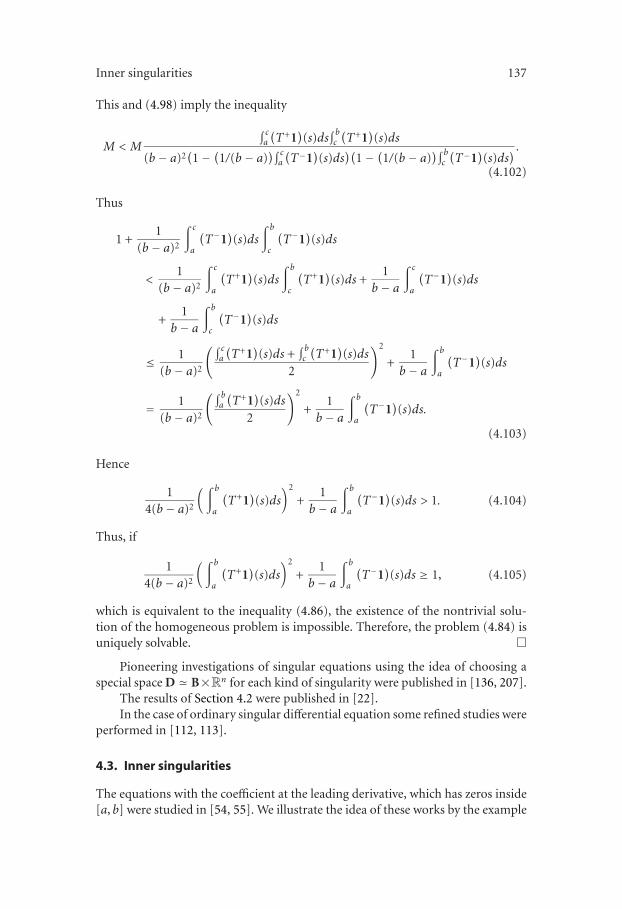
Inner singularities 137
This and (4.98) imply the inequality
M < M
∫ ca
(T+1
)(s)ds
∫ bc
(T+1
)(s)ds
(b− a)2(1− (1/(b− a)
)∫ ca
(T−1
)(s)ds
)(1− (1/(b − a)
)∫ bc
(T−1
)(s)ds
) .
(4.102)
Thus
1 +1
(b− a)2
∫ c
a
(T−1
)(s)ds
∫ b
c
(T−1
)(s)ds
<1
(b− a)2
∫ c
a
(T+1
)(s)ds
∫ b
c
(T+1
)(s)ds +
1b − a
∫ c
a
(T−1
)(s)ds
+1
b − a∫ b
c
(T−1
)(s)ds
≤ 1(b− a)2
(∫ ca
(T+1
)(s)ds +
∫ bc
(T+1
)(s)ds
2
)2
+1
b − a∫ b
a
(T−1
)(s)ds
= 1(b− a)2
(∫ ba
(T+1
)(s)ds
2
)2
+1
b − a∫ b
a
(T−1
)(s)ds.
(4.103)
Hence
14(b − a)2
(∫ b
a
(T+1
)(s)ds
)2
+1
b− a∫ b
a
(T−1
)(s)ds > 1. (4.104)
Thus, if
14(b− a)2
(∫ b
a
(T+1
)(s)ds
)2
+1
b − a∫ b
a
(T−1
)(s)ds ≥ 1, (4.105)
which is equivalent to the inequality (4.86), the existence of the nontrivial solu-tion of the homogeneous problem is impossible. Therefore, the problem (4.84) isuniquely solvable. �
Pioneering investigations of singular equations using the idea of choosing aspecial space D � B×Rn for each kind of singularity were published in [136, 207].
The results of Section 4.2 were published in [22].In the case of ordinary singular differential equation some refined studies were
performed in [112, 113].
4.3. Inner singularities
The equations with the coefficient at the leading derivative, which has zeros inside[a, b] were studied in [54, 55]. We illustrate the idea of these works by the example
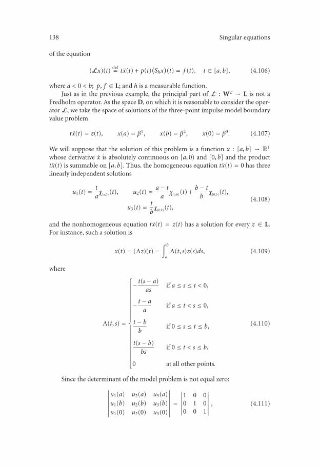
138 Singular equations
of the equation
(Lx)(t)def= tx(t) + p(t)
(Shx)(t) = f (t), t ∈ [a, b], (4.106)
where a < 0 < b; p, f ∈ L; and h is a measurable function.Just as in the previous example, the principal part of L : W2 → L is not a
Fredholm operator. As the space D, on which it is reasonable to consider the oper-ator L, we take the space of solutions of the three-point impulse model boundaryvalue problem
tx(t) = z(t), x(a) = β1, x(b) = β2, x(0) = β3. (4.107)
We will suppose that the solution of this problem is a function x : [a, b] → R1
whose derivative x is absolutely continuous on [a, 0) and [0, b] and the producttx(t) is summable on [a, b]. Thus, the homogeneous equation tx(t) = 0 has threelinearly independent solutions
u1(t) = t
aχ[a,0) (t), u2(t) = a− t
aχ[a,0) (t) +
b − tb
χ[0,b] (t),
u3(t) = t
bχ[0,b] (t),
(4.108)
and the nonhomogeneous equation tx(t) = z(t) has a solution for every z ∈ L.For instance, such a solution is
x(t) = (Λz)(t) =∫ b
aΛ(t, s)z(s)ds, (4.109)
where
Λ(t, s) =
⎧⎪⎪⎪⎪⎪⎪⎪⎪⎪⎪⎪⎪⎪⎪⎪⎪⎪⎪⎪⎪⎪⎨
⎪⎪⎪⎪⎪⎪⎪⎪⎪⎪⎪⎪⎪⎪⎪⎪⎪⎪⎪⎪⎪⎩
− t(s− a)as
if a ≤ s ≤ t < 0,
− t − aa
if a ≤ t < s ≤ 0,
t − bb
if 0 ≤ s ≤ t ≤ b,
t(s− b)bs
if 0 ≤ t < s ≤ b,
0 at all other points.
(4.110)
Since the determinant of the model problem is not equal zero:
∣∣∣∣∣∣∣∣
u1(a) u2(a) u3(a)u1(b) u2(b) u3(b)u1(0) u2(0) u3(0)
∣∣∣∣∣∣∣∣=∣∣∣∣∣∣∣
1 0 00 1 00 0 1
∣∣∣∣∣∣∣
, (4.111)
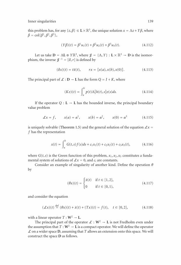
Inner singularities 139
this problem has, for any {z,β} ∈ L×R3, the unique solution x = Λz+Yβ, whereβ = col{β1,β2,β3},
(Yβ)(t) = β1u1(t) + β2u2(t) + β3u3(t). (4.112)
Let us take D = ΛL ⊕ YR3, where J = {Λ,Y} : L × R3 → D is the isomor-phism, the inverse J−1 = [δ, r] is defined by
(δx)(t) = tx(t), rx = {x(a), x(b), x(0)}. (4.113)
The principal part of L : D → L has the form Q = I + K , where
(Kz)(t) =∫ b
ap(t)Λ
[h(t), s
]z(s)ds. (4.114)
If the operator Q : L → L has the bounded inverse, the principal boundaryvalue problem
Lx = f , x(a) = α1, x(b) = α2, x(0) = α3 (4.115)
is uniquely solvable (Theorem 1.5) and the general solution of the equation Lx =f has the representation
x(t) =∫ b
aG(t, s) f (s)ds + c1x1(t) + c2x2(t) + c3x3(t), (4.116)
where G(t, s) is the Green function of this problem, x1, x2, x3 constitutes a funda-mental system of solutions of Lx = 0, and ci are constants.
Consider an example of singularity of another kind. Define the operation θby
(θx)(t) =⎧⎨
⎩
x(t) if t ∈ [1, 2],
0 if t ∈ [0, 1),(4.117)
and consider the equation
(Lx)(t)def= (θx)(t) + x(t) + (Tx)(t) = f (t), t ∈ [0, 2], (4.118)
with a linear operator T : W2 → L.The principal part of the operator L : W2 → L is not Fredholm even under
the assumption that T : W2 → L is a compact operator. We will define the operatorL on a wider space D, assuming that T allows an extension onto this space. We willconstruct the space D as follows.
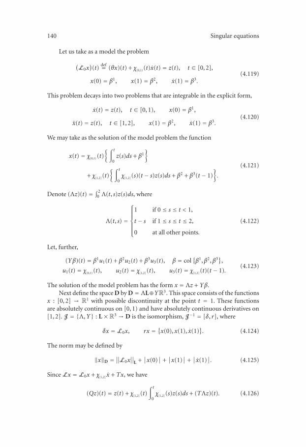
140 Singular equations
Let us take as a model the problem
(L0x
)(t)
def= (θx)(t) + χ[0,1) (t)x(t) = z(t), t ∈ [0, 2],
x(0) = β1, x(1) = β2, x(1) = β3.(4.119)
This problem decays into two problems that are integrable in the explicit form,
x(t) = z(t), t ∈ [0, 1), x(0) = β1,
x(t) = z(t), t ∈ [1, 2], x(1) = β2, x(1) = β3.(4.120)
We may take as the solution of the model problem the function
x(t) = χ[0,1) (t){∫ t
0z(s)ds + β1
}
+ χ[1,2] (t){∫ t
0χ[1,2] (s)(t − s)z(s)ds + β2 + β3(t − 1)
}.
(4.121)
Denote (Λz)(t) = ∫ 20 Λ(t, s)z(s)ds, where
Λ(t, s) =
⎧⎪⎪⎪⎪⎨
⎪⎪⎪⎪⎩
1 if 0 ≤ s ≤ t < 1,
t − s if 1 ≤ s ≤ t ≤ 2,
0 at all other points.
(4.122)
Let, further,
(Yβ)(t) = β1u1(t) + β2u2(t) + β3u3(t), β = col{β1,β2,β3},
u1(t) = χ[0,1) (t), u2(t) = χ[1,2] (t), u3(t) = χ[1,2] (t)(t − 1).(4.123)
The solution of the model problem has the form x = Λz + Yβ.Next define the space D by D = ΛL⊕YR3. This space consists of the functions
x : [0, 2] → R1 with possible discontinuity at the point t = 1. These functionsare absolutely continuous on [0, 1) and have absolutely continuous derivatives on[1, 2]. J = {Λ,Y} : L×R3 → D is the isomorphism, J−1 = [δ, r], where
δx = L0x, rx = {x(0), x(1), x(1)}. (4.124)
The norm may be defined by
‖x‖D =∥∥L0x
∥∥
L +∣∣x(0)
∣∣ +
∣∣x(1)
∣∣ +
∣∣x(1)
∣∣. (4.125)
Since Lx = L0x + χ[1,2] x + Tx, we have
(Qz)(t) = z(t) + χ[1,2] (t)∫ t
0χ[1,2] (s)z(s)ds + (TΛz)(t). (4.126)
Inner singularities 141
If the product TΛ : L → L is compact, the principal part Q : L → L is canonicalFredholm. If ‖K‖L→L < 1, where
(Kz)(t) = (TΛz)(t) + χ[1,2] (t)∫ t
0χ[1,2] (s)z(s)ds, (4.127)
the principal boundary value problem
Lx = f , x(0) = α1, x(1) = α2, x(1) = α3 (4.128)
is uniquely solvable and in this case (Theorem 1.6) the homogeneous equationLx = 0 has three-dimensional fundamental system of solutions x1, x2, x3, alsothe general solution of the equation Lx = f in the space D has the representation
x(t) =∫ 2
0G(t, s) f (s)ds + c1x1(t) + c2x2(t) + c3x3(t), (4.129)
where G(t, s) is the Green function of the principal boundary value problem, ci =const.
Denote Δx(t) = x(t)− x(t − 0). The constriction D0 = {x ∈ D : Δx(1) = 0}of the space D contains continuous functions only. The homogeneous equationL0x = 0 has two linearly independent solutions
y1(t) = 1− χ[1,2] (t)(t − 1), y2(t) = χ[1,2] (t)(t − 1) (4.130)
in the space D0. The equation L0x = z has, for any z ∈ L, solutions that belong toD0, for instance,
v(t) = χ[0,1) (t)∫ t
0z(s)ds + χ[1,2] (t)
{∫ t
0χ[1,2] (s)(t − s)z(s)ds +
∫ 1
0z(s)ds
}. (4.131)
Thus, the general solution of the model equation L0x = z in the space D0 may berepresented in the form
x(t) = v(t) + c1y1(t) + c2y2(t), (4.132)
where c1, c2 are constants.Since
∣∣∣∣∣y1(0) y2(0)y1(2) y2(2)
∣∣∣∣∣ =
∣∣∣∣∣
1 00 1
∣∣∣∣∣ �= 0, (4.133)
the two-point boundary value problem
L0x = z, x(0) = 0, x(2) = 0 (4.134)
142 Singular equations
is uniquely solvable in the space D0. The Green function of this problem, W(t, s),can be constructed by finding the constants c1, c2 in (4.132) so that x(0) = x(2) =0. We have
x(t)def= (Wz)(t) =
∫ 2
0W(t, s)z(s)ds, (4.135)
where
W(t, s) =
⎧⎪⎪⎪⎪⎪⎪⎪⎪⎪⎪⎪⎨
⎪⎪⎪⎪⎪⎪⎪⎪⎪⎪⎪⎩
1 if 0 ≤ s ≤ t < 1,
2− t if 1 ≤ t ≤ 2, 0 ≤ s < 1,
−(2− t)(s− 1) if 1 ≤ s ≤ t ≤ 2,
−(2− s)(t − 1) if 1 ≤ t < s ≤ 2,
0 at all other points.
(4.136)
Notice that it is possible to construct W(t, s) on the base of the representation
x(t) = (Λz)(t) + β1u1(t) + β2u2(t) + β3u3(t) (4.137)
of the solution (4.119) by demanding the fulfillment of the conditions x(0) =Δx(1) = x(2) = 0.
Thus, the space D0 is defined by D0 =WL⊕ Y0R2, where
(Y0β
)(t) = [1− χ[1,2] (t)(t − 1)
]β1 + χ[1,2] (t)(t − 1)β2, β = col
{β1,β2},
(4.138)
J0={W ,Y0} : L×R2 → D0 is the isomorphism, J−10 =[L0, r0], r0x={x(0), x(2)}.
The two-point boundary value problem
Lx = f , x(0) = α1, x(2) = α2 (4.139)
is the principal boundary value problem for the equation Lx = f in the space D0.This problem is uniquely solvable if and only if the operator Q = LW : L → L hasthe bounded inverse.
4.4. The chemical reactor’s equation
The mathematical description of some processes in chemical reactors gives rise tothe singular boundary value problem
x(t) +k
tx(t) = f (t, x), t ∈ [0, 1], x(0) = 0, x(1) = α. (4.140)
The chemical reactor’s equation 143
There is an extensive literature on the subject (see, e.g., [169, 224]). Application ofthe method of “L1, L2—quasilinearization” (see [32]) to this problem demandsthe tests of solvability of the linear problem
(Lx)(t)def= x(t) +
k
tx(t) + p(t)x(t) = f (t), t ∈ [0, 1],
x(0) = 0, x(1) = α(4.141)
and of antitonicy of the Green operator of the problem. We will follow below thescheme suggested by Alves [5].
The value of the operator L on a function whose derivative differs from zeroat the point t = 0 (e.g., x(t) = t) does not belong to the space of summablefunctions. Thus it is natural to consider the equation Lx = f in a space wherethere are no such functions. Let us consider the equation Lx = f in the space Dof functions x : [0, 1] → R1 defined by
x(t) =∫ t
0(t − s)z(s)ds + β, {z,β} ∈ Lp ×R
1, (4.142)
where Lp is the Banach space of functions z : [0, 1] → R1 under the norm
‖z‖Lp ={∫ 1
0
∣∣z(s)∣∣pds
}1/p
. (4.143)
We will demand below the inequalities p > 1 and k > −(p − 1)/p.The space D is a finite-dimensional restriction of the space W2
p of the func-tions with absolutely continuous derivative and the second derivative from Lp.Namely
D = {x ∈ W2p : x(0) = 0
}. (4.144)
Such a space is isomorphic to the product Lp × R1, the isomorphism may be de-fined, for instance, by
J = {Λ,Y}, (Λz)(t) =∫ t
0(t − s)z(s)ds, Yβ = β,
J−1 = [δ, r], δx = x, rx = x(0).(4.145)
The equation
(Mx)(t)def= x(t) +
k
tx(t) = f (t), t ∈ [0, 1], (4.146)
is integrable in the explicit form and may be taken as a model one. The principal
144 Singular equations
part QM =MΛ of the operator M : D → Lp has the form
QMz = z + Kz, (4.147)
where
(Kz)(t) = k
t
∫ t
0z(s)ds. (4.148)
This is the so-called Cezaro operator. As one can make sure by immediate integra-tion of the integral equation z + Kz = f , the inverse Q−1
M = (I + K)−1 : Lp → Lp
has the representation
(Q−1M f
)(t) = f (t)− kt−(1+k)
∫ t
0sk f (s)ds (4.149)
and is bounded if k > −(p − 1)/p.It should be noticed that K : Lp → Lp is not compact and the successive ap-
proximations in the case k ≥ 1 do not converge. One can see the fact by beginningthe successive approximations from the element z0 = 1. This phenomenon un-expected from the view-point of the accustomed properties of Volterra integralequations is connected with characteristics of the Cezaro operator K : Lp → Lp
whose spectrum was studied in [162].So, the principal part QM : Lp → Lp of M : D → Lp as well the inverse Q−1
M arebounded Volterra. By Theorem 1.16, the Cauchy problem Mx = f , x(0) = 0 (theprincipal boundary value problem), is uniquely solvable . By virtue of Theorem1.17 the fundamental system of Mx = 0 is one-dimensional and consists of x(t) ≡1. Thus the general solution of the equation Mx = f has the form
x(t) = (ΛQ−1M f
)(t) + α = (CM f
)(t) + α, (4.150)
where
(CM f
)(t) =
∫ t
0CM(t, s) f (s)ds (4.151)
and the Cauchy function CM(t, s) is defined by
CM(t, s) = t − s− ksk∫ t
0(t − τ)τ−(1+k)dτ, 0 ≤ s ≤ t ≤ 1. (4.152)
Thus,
CM(t, s) = s lnt
s, CM(0, 0) = 0 (4.153)
The chemical reactor’s equation 145
in the case k = 1 and
CM(t, s) = s
k − 1
[
1−(s
t
)k−1]
, CM(0, 0) = 0 (4.154)
in the case k �= 1.It should be noticed that the operator CM : Lp → C defined by (4.151) is
compact being the product of the compact Λ : Lp → C and the bounded Q−1M :
Lp → Lp.The boundary value problem Mx = f , lx = α for any functional l on the
space D, such that l(1) �= 0, is uniquely solvable and its Green function GM(t, s)may be constructed in the explicit form on the base of the equality that followsfrom Theorem 1.20:
GM(t, s) = CM(t, s)− 1l(1)
l[CM(·, s)], (4.155)
where CM(t, s) = 0 if a ≤ t < s ≤ b. Thus the Green function of the problem
x +k
tx = f , x(1) = 0 (4.156)
is defined by
GM(t, s) =⎧⎨
⎩s ln t if 0 ≤ s ≤ t ≤ 1,
s ln s if 0 ≤ t < s ≤ 1,(4.157)
in the case k = 1, and by
GM(t, s) =
⎧⎪⎪⎪⎪⎨
⎪⎪⎪⎪⎩
sk(t1−k − 1
)
1− k if 0 ≤ s ≤ t ≤ 1,
sk(s1−k − 1
)
1− k if 0 ≤ t < s ≤ 1,
(4.158)
in the case k �= 1.Next consider the problem
(Lx)(t)def= x(t) +
k
tx(t) + p(t)x(t) = f (t), x(1) = α (4.159)
with p ∈ Lp.
Theorem 4.20. The following assertions are equivalent.(a) The problem (4.159) is uniquely solvable in the space D and its Green op-
erator is antitonic.
146 Singular equations
(b) There exists v ∈ D such that
v(t) ≥ 0, (Lv)(t) ≤ 0, t ∈ [0, 1], (4.160)
and besides
v(1)−∫ 1
0(Lv)(s)ds > 0. (4.161)
(c) There exists the positive solution of the homogeneous equation Lx = 0.
Beforehand, let us prove two auxiliary lemmas using the following designa-tions: p = p+ − p−, p+(t), p−(t) ≥ 0, L0x = x + (k/t)x − p−x.
Lemma 4.21. The Cauchy problem
L0x = f , x(0) = α (4.162)
is uniquely solvable in the space D, the Cauchy operator C0 of the equation L0x =f is isotonic, and there exists the positive solution u0 of the homogeneous equationL0x = 0.
Proof. The problem (4.162) is equivalent to the equation
x = Hx + g, (4.163)
where
(Hx)(t) =∫ t
0CM(t, s)p−(s)x(s)ds, g(t) =
∫ t
0CM(t, s) f (s)ds + α. (4.164)
The operatorH : C → C is Volterra, compact, and isotonic. Therefore the problem(4.162) is uniquely solvable and the Cauchy operator of the problem
C0 =(I +H +H2 + · · · )CM (4.165)
is also isotonic. The function u0 as the solution of the equation x = Hx+ 1 has therepresentation
u0 = 1 +H(1) +H2(1) + · · · (4.166)
and, consequently, u0(t) ≥ 1, t ∈ [0, 1]. �
Lemma 4.22. The boundary value problem
L0x = f , x(1) = 0 (4.167)
is uniquely solvable in the space D and its Green operator W is antitonic.
The chemical reactor’s equation 147
Proof. The homogeneous problem L0x = 0, x(1) = 0 is equivalent to the equa-tion x = Bx with antitonic
(Bx)(t) =∫ 1
0GM(t, s)p−(s)x(s)ds. (4.168)
If we assume that the problem is not uniquely solvable, then it follows that thereexists the nontrivial solution y of the problem. In virtue of antitonicity of B, thenontrivial solution varies the sign on [0, 1]. Thus y has at least two zeros t = 1 andt = τ. The case that τ = 0 is impossible since in this case, we have y(t) ≡ 0 byLemma 4.21.
Consider now the regular equation
x(t) +k
tx(t)− p−(t)x(t) = 0, t ∈ [τ, 1]. (4.169)
The fundamental system of this equation is nonoscillatory on [τ, 1]. It followsfrom Theorem D.1 if we put v(t) ≡ 1. Thus, y(τ) �= 0. The contradiction provesthe unique solvability of the problem (4.167).
Assume that the Green operator W of the problem (4.167) is not antitonicand f (t) ≥ 0 is a function such that the solution x =W f takes positive values ona set of points from [0, 1]. If x(0) = γ ≥ 0, the function x, as the solution of theCauchy problem
L0x = f , x(0) = γ, (4.170)
does not satisfy the condition x(1) = 0 of the boundary value problem. Really, iff (t) ≥ 0,
x(1) =∫ 1
0C0(1, s) f (s)ds + γ > 0 (4.171)
since C0(1, s) ≥ CM(1, s) > 0, s ∈ (0, 1), by virtue of (4.165). If x(0) < 0, thesolution x =W f has a pair of zeros τ1, τ2 ∈ (0, 1] such that x(t) > 0, t ∈ (τ1, τ2).On the segment [τ1, τ2] the function x = W f satisfies the two-point boundaryvalue problem
(Vx)(t)def= x(t) +
k
tx(t)−p−(t)x(t) = f (t), t ∈ [τ1, τ2
],
x(τ1) = x
(τ2) = 0.
(4.172)
Since (V[1])(t) = −p−(t) ≤ 0, the solution x of this problem does not take posi-tive values by virtue of Theorem D.1. The contradiction completes the proof. �
Now the proof of Theorem 4.20 follows at once from Theorem D.2. Indeed,Lemmas 4.21 and 4.22 guarantee the fulfillment of the assumptions of this theo-rem as applied to the problem
(Lx)(t) ≡ (L0x)(t) + p+(t)x(t) = f (t), x(1) = 0. (4.173)

5Minimization of square functionals
5.1. Introduction
The problem of minimization of functionals is unsolvable in the frame of the clas-sical calculus of variations if the given functional has no minimum on the tradi-tional sets of functions. The question about the suitable choice of the set on whichthe functional must be defined was posed by Hilbert and, as it was emphasized bythe authors of the book of Alekseev et al. [3], therewith each class of functionalsmust be studied in its own proper space.
The classical calculus of variations usually deals with the functionals of theform
∫ b
a(Φx)(s)ds (5.1)
with a local operator Φ : Wn → L. The results of Chapter 1 enables us to study thefunctional with more general operator Φ : Wn → L and replace the space Wn by amore suitable “own” space D � B×Rn.
The scheme proposed below permits approaching a new fashion to the prob-lem of minimization, it extends the capabilities of the calculus of variations andleads to sufficient tests of the existence of the minimum for some classes of func-tionals in the terms of the problem.
The scheme has been developed on the base of the theory of abstract func-tional differential equations in the works of the Perm Seminar.
5.2. The criterion for the existence of the minimum ofthe square functional
Let D be a Banach space of functions x : [a, b] → R1, which is isomorphic to thedirect product L2 ×Rn, let L2 be the Banach space of square summable functions
z : [a, b] → R1, ‖z‖L2 = {∫ ba z
2(s)ds}1/2.
150 Minimization of square functionals
Consider the problem on the existence of an element x ∈ D at which thesquare functional
I(x) = 12
∫ b
a
{ m∑
i=1
(T1ix
)(s)(T2ix
)(s) +
(T0x
)(s) + ω(s)
}
ds (5.2)
with additional conditions
lix = αi, i = 1, . . . ,n, (5.3)
reaches the minimum.Here Tji : D → L2, j = 1, 2, i = 1, . . . ,m, and T0 : D → L2 are linear bounded
operators, l1, . . . , ln is a system of linear bounded, linearly independent functionalson D, and ω is a summable function.
We will rewrite such a problem in the form
I(x) �→ min,
lx = α,(5.4)
where l = [l1, . . . , ln], α = {α1, . . . ,αn}.
5.2.1. The reduction of the problem in the space D � L2 ×Rn
to a problem in the space L2
Suppose that the isomorphism J = {Λ,Y} : L2 ×Rn → D is constructed accord-ing to a given system of functionals l1, . . . , ln on the base of a uniquely solvableboundary value problem
δx = z, lix = βi, i = 1, . . . ,n, (5.5)
with linear δ : D → L2. Such an operator exists by virtue of Theorem 1.22. Thus, Λis the Green operator of the problem (5.5), Y = {y1, . . . , yn}, y1, . . . , yn constitutethe fundamental system of the homogeneous equation δx = 0.
The problem under consideration may be reduced, by means of the substitu-tion
x = Λz + Yα, (5.6)
to the problem of the minimization of the functional
I1(z)def= I(Λz + Yα) (5.7)
The criterion for the existence of the minimum of the square functional 151
over the Hilbert space L2 without additional conditions. Denoting Yα = u, Qji =TjiΛ, Q0 = T0Λ, we have
I(x) = I(Λz + u)def= I1(z)
= 12
∫ b
a
m∑
i=1
(Q1iz
)(s)(Q2iz
)(s)ds
+12
∫ b
a
m∑
i=1
{(Q1iz
)(s)(T2iu
)(s) +
(Q2iz
)(s)(T1iu
)(s)}ds
+12
∫ b
a
m∑
i=1
(T1iu
)(s)(T2iu
)(s)ds
+12
∫ b
a
{(Q0z
)(s) +
(T0u
)(s)}ds +
12
∫ b
aω(s)ds.
(5.8)
Using the equality
∫ b
a(Az)(s)(Bz)(s)ds =
∫ b
a
(A∗Bz
)(s)z(s)ds (5.9)
and denoting
〈ϕ,ψ〉 =∫ b
aϕ(s)ψ(s)ds, (5.10)
we may write
I1(z) = 12〈Hz, z〉 − 〈θ, z〉 + g, (5.11)
where
H = 12
m∑
i=1
(Q∗1iQ2i +Q∗2iQ1i
),
θ = −12
m∑
i=1
(Q∗1iT2i +Q∗2iT1i
)u− 1
2Q∗0 (1),
g = 12
∫ b
a
{ m∑
i=1
(T1iu
)(s)(T2iu
)(s) +
(T0u
)(s) + ω(s)
}
ds.
(5.12)
Thus H : L2 → L2 is a selfadjoint operator, θ ∈ L2, g = const.Denote
Dα ={x ∈ D : lix = αi, i = 1, . . . ,n
}. (5.13)
152 Minimization of square functionals
To state and prove the central assertion on the minimum of the functional (5.2),we will use the following definitions.
A point x0 ∈ Dα (z0 ∈ L2) is called the point of local minimum of functionalI (I1) if there exists an ε > 0 such that I(x) ≥ I(x0) (I1(z) ≥ I1(z0)) for allx ∈ Dα (z ∈ L2) that satisfy ‖x − x0‖D < ε (‖z − z0‖L2 < ε). If I(x) ≥ I(x0)(I1(z) ≥ I1(z0)) holds for all x ∈ Dα (z ∈ L2), x0 (z0) is called the point ofglobal minimum. The value I(x0) (I1(z0)) is called local (global) minimum of thefunctional.
Following the adopted terminology, we will call the operator H : L2 → L2
positive definite one if 〈Hz, z〉 ≥ 0 for all z ∈ L2. The positive definite operator His called strictly positive definite if 〈Hz, z〉 = 0 only for z = 0.
Denote
L = 12
m∑
i=1
(Q∗1iT2i +Q∗2iT1i
), θ0 = −1
2Q∗0(
1). (5.14)
Theorem 5.1. Any local minimum of the functional (5.2) is the global one.A point x0 ∈ Dα is the point of minimum of the functional (5.2) if and only if
(a) x0 is a solution of the boundary value problem
Lx = θ0, lix = αi, i = 1, . . . ,n, (5.15)
(b) the operator H : L2 → L2 defined by (5.12) is positive definite.
Remark 5.2. The equation Lx = θ0 is naturally called “Euler equation” and theboundary conditions lix = αi correspond to “natural boundary conditions” in theclassical calculus of variations.
5.2.2. Proof of Theorem 5.1
As a preliminary we will proof the following auxiliary statements.
Lemma 5.3. Any local minimum of the functional I1 on the space L2 is the globalone.
An element z0 ∈ L2 is the point of minimum of I1 if and only if the operatorH : L2 → L2 defined by (5.12) is positive definite and z0 is a solution to the equationHz = θ.
Proof. Let z0 be a point of a local minimum. It means that there exists an ε > 0such that I1(z)− I1(z0) ≥ 0 for ‖z − z0‖L2 < ε. Let us fix ξ ∈ L2 and let γ0 > 0 bea number such that ‖γ0ξ‖L2 < ε. It follows from (5.11) that
I1(z0 + γξ
)− I1(z0) = γ2
2〈Hξ, ξ〉 + γ
⟨Hz0 − θ, ξ
⟩. (5.16)
Due to the condition, the quadratic binomial (γ2/2)〈Hξ, ξ〉 + γ〈Hz0 − θ, ξ〉 hasno negative value if γ ∈ (−γ0, γ0). It means that this binomial has no negative
The criterion for the existence of the minimum of the square functional 153
value for any γ. Consequently, z0 is a point of global minimum. Besides, due to thearbitrary choice of ξ, we obtain from the equality 〈Hz0−θ, ξ〉 = 0 thatHz0−θ = 0.Then 〈Hξ, ξ〉 ≥ 0 for each ξ ∈ L2.
The converse assertion follows from (5.16). �
Lemma 5.4. If x0 is the point of a local minimum of the functional (5.2) on the setDα and x0 = Λz0 + u, then the point of minimum of the functional I1 is z0.
Proof. Let ε > 0 be such that I(x) − I(x0) ≥ 0, as soon as ‖x − x0‖D < ε. Anyx ∈ Dα has the representation x = Λz + u. Since ‖x − x0‖D ≤ ‖Λ‖‖z − z0‖L2 , wehave
I1(z)− I1(z0) = I(x)− I
(x0) ≥ 0 for
∥∥z − z0
∥∥
L2≤ ε
‖Λ‖ . (5.17)
Hence z0 is a point of minimum of the functional I1. �From the equality I(x) − I(x0) = I1(z) − I1(z0) for x0 = Λz0 + u and for
x = Λz + u, it follows at once that x0 is the point of the global minimum of thefunctional I if and only if z0 is the point of global minimum of the functional I1.From this and previous lemmas we obtain the following.
Lemma 5.5. Any local minimum of the functional I is the global one.The functional I has a point of minimum x0 on the set Dα = {x ∈ D : lix =
αi, i = 1, . . . ,N} if and only if the operator H : L2 → L2 defined by (5.12) is positivedefinite and Hz = θ has a solution z0 ∈ L2. In this case, x0 = Λz0 + u.
Corollary 5.6. Let the operator H defined by (5.12) be of the form H = I − K . Thefunctional (5.2) with restrictions (5.3) has the unique minimum in D andH is strictlypositive definite if ‖K‖ < 1.
Proof. The inequality ‖K‖ < 1 implies that the equation Hz = θ has the uniquesolution z0. Besides, this inequality guarantees that H is positive definite since
〈Hz, z〉 = 〈z, z〉 − 〈Kz, z〉 ≥ ‖z‖2L2− ‖K‖‖z‖2
L2≥ 0. (5.18)
By Lemma 5.5, x0 = Λz0 +u is the point of the unique minimum of the functionalon the set Dα. �Proof of Theorem 5.1. Let x0 ∈ Dα be the solution of the problem (5.15). Thereexists z0 ∈ L2 such that x0 = Λz0 + u. Moreover
Hz0 = LΛz0 = L(x0 − u
) = θ0 + θ − θ0 = θ. (5.19)
Consequently, z0 is the solution to the equation Hz = θ. By virtue of Lemma 5.5,x0 is the point of minimum.
154 Minimization of square functionals
Conversely, if x0 is the point of minimum of the functional I and x0 = Λz +u, z0 is the point of minimum of the functional I1. By virtue of Lemma 5.3 theoperator H is positive definite and Hz0 − θ = 0.
Let us show that x0 is the solution of the problem (5.15). Indeed, lx0 = α,
Lx0 = L(Λz0 + u
) = Hz0 − θ + θ0 = θ0. (5.20)�
Remark 5.7. In some instances the equation Hz = θ is more convenient for thestudy than the boundary value problem (5.15). In such cases there is a good reasonto use Lemma 5.5 instead of Theorem 5.1.
5.2.3. A simple example
Consider the functional
I(x) = 12
∫ 1
0
{x2(s)− q(s)x(s)− p(s)x(s)
}ds (5.21)
with conditions x(0) = α1, x(1) = α2.If q is absolutely continuous, the classical methods from elementary textbooks
is applicable. The classical Euler equation in this case has the form
x(t) = 12
[q(t)− p(t)
](5.22)
and, therefore, the point of minimum is defined by
x0(t) = 12
∫ 1
0W(t, s)
[q(s)− p(s)
]ds + α1(1− t) + α2t, (5.23)
where
W(t, s) =⎧⎨
⎩
−s(1− t) if 0 ≤ s ≤ t ≤ 1,
−t(1− s) if 0 ≤ t < s ≤ 1,(5.24)
is the Green function of the problem x = z, x(0) = 0, x(1) = 0. Thus
x0(t) = 12
[∫ t
0q(s)ds− t
∫ 1
0q(s)ds− (t − 1)
∫ t
0sp(s)ds− t
∫ 1
t(s− 1)p(s)ds
]
+ α1(1− t) + α2t.(5.25)
Note that I(x0) = −p2/96 if α1 = α2 = 0, p = const, q = const.Next consider the same problem using the scheme above. Let D � L2 × R2
and let J = {Λ,Y} : L2 ×Rn → D be the isomorphism.
The criterion for the existence of the minimum of the square functional 155
Since T11x = T21xdef= Tx = x, T0x = −qx − px, we have Q11 = Q12 = TΛ
def=Q, H = Q∗Q. In any case of D (for every Λ) the operator H : L2 → L2 is positivedefinite since
〈Hz, z〉 = ⟨Q∗Qz, z〉 = 〈Qz,Qz〉. (5.26)
Let D = W22 be the space of the functions x : [a, b] → R with absolutely
continuous derivative x and x ∈ L2. Define the isomorphism J = {Λ,Y} : L2 ×R2 → W2
2 by
(Λz)(t) =∫ 1
0W(t, s)z(s)ds, (Yβ)(t) = β1(1− t) + β2t, β = col
{β1,β2}
(5.27)
with W(t, s) defined by (5.24). Thus
(Λz)(t) = (t − 1)∫ t
0sz(s)ds− t
∫ 1
t(1− s)z(s)ds. (5.28)
After direct calculations, we have
(Qz)(t) = −∫ 1
tz(s)ds +
∫ 1
0sz(s)ds,
(Q∗z
)(t) = −
∫ t
0z(s)ds + t
∫ 1
0z(s)ds,
(Q0z
)(t) = q(t)
∫ 1
tz(s)ds− q(t)
∫ 1
0sz(s)ds + (1− t)p(t)
∫ t
0sz(s)ds
+ tp(t)∫ 1
t(1− s)z(s)ds,
(Q∗0 z
)(t) =
∫ t
0q(s)z(s)ds− t
∫ 1
0q(s)z(s)ds + t
∫ 1
t(1− s)p(s)z(s)ds
+ (1− t)∫ t
0sp(s)z(s)ds,
θ0(t) = 12
{−∫ t
0q(s)ds + t
∫ 1
0q(s)ds + t
∫ 1
t(s− 1)p(s)ds + (t − 1)
∫ t
0sp(s)ds
}.
(5.29)
Next L = Q∗T and the equation Lx = θ0 takes the form
−x(t) + x(0) + tx(1)− tx(0) = θ0. (5.30)
By Theorem 5.1, the unique point of minimum is again the function (5.25).Let us notice that after double differentiation, the equation Lx = θ0 takes the
form of the classical Euler equation (5.22).By immediate differentiation we see that x0 ∈ W2
2 if and only if p, q ∈ L2.Therefore, the functional (5.21) has no minimum in W2
2 without this condition.
156 Minimization of square functionals
If we restrict ourselves to the requirement p, q ∈ L2, it is natural to look forthe minimum in a space being wider than W2
2.Consider the problem in the space D � L2 × R2 of the functions x : [0, 1] →
R1 which are absolutely continuous on [0, c) and [c, 1] and such that x ∈ L2.The isomorphism between D and L2 × R2 may be constructed on the base of theimpulse boundary value problem
x(t) = z(t), x(0) = β1, x(1) = β2 (5.31)
in the space D. The solution of this problem has the form
x(t) = (Λz)(t) + (Yβ)(t)
def=∫ t
0z(s)ds− χ[c,1](t)
∫ 1
0z(s)ds + β1χ[0,c)(t) + β2χ[c,1](t).
(5.32)
Then Qz = Q∗z = z, Hz = z,
(Q∗0 z
)(t) = 1
2
{− q(t)z(t) +
∫ t
cp(s)z(s)ds
}. (5.33)
Let α1 = α2 = 0. Then
θ(t) = 12
{q(t)−
∫ t
cp(s)ds
}. (5.34)
The solution to Hz = θ has the form z0 = θ and the functional I has its minimumat the point
x0(t) = (Λθ)(t)
= 12
{∫ t
0q(s)ds +
∫ t
0sp(s)ds− t
∫ t
cp(s)ds
− χ[c,1](t)
[∫ 1
0q(s)ds +
∫ 1
0sp(s)ds−
∫ 1
cp(s)ds
]}
.
(5.35)
If p and q are constants, then
I(x0) = −1
8
[q2 + pq(2c − 1) + p2
(c2 − c +
13
)]. (5.36)
Thus the minimum depends on the position of c, the point of discontinuity. Ifq = 0, I(x0) = −(1/8)p2(c2 − c + 1/3), I(x0) = −p2/96 for c = 1/2. If c → 0 orc → 1, then I(x0) → −p2/24.
The tests of the existence of the minimum of the functional 157
5.3. The tests of the existence of the minimum of the functional
5.3.1. Some properties of the selfadjoint operators in L2
It is known that the selfadjoint H : L2 → L2 is positive definite if and only if thespectrum of H , σ(H), does not contain negative numbers: σ(H) ⊂ [0, +∞). If theoperator H is strictly positive definite and moreover is Fredholm, then σ(H) ⊂(0, +∞). Indeed, in this event the equation Hz = 0 has only the trivial solutionand, consequently, there exists the bounded inverse H−1. Thus the number 0 is aregular value to H .
For the selfadjoint H arising in studying the functional (5.2), the situationH = H0−H1 is typical whereH0 andH1 are bounded, selfadjoint, positive definite,there exists the bounded inverse H−1
0 and H1 is compact. It should be noticed thatin this case H is Fredholm as the sum of an invertible operator and a compact one.Let us dwell on such a situation.
It is known that there exists the only square root√H0 (such that (
√H0)2 = H0)
for the positive definiteH0 and, besides,√H0 permutes withH0 and with any other
operator that is permutable with H0 (see [108]).
Lemma 5.8. Let H0 be positive definite and there exists the bounded inverse H−10 .
Then there exists the bounded inverse (√H0)−1 and, besides, (
√H0)−1 =
√H−1
0 .
Proof. H−10 is positive definite. Consequently, there exists
√H−1
0 and it permutes
with H−10 . Since H−1
0 permutes with H0 and√H0, the operators
√H−1
0 and√H0
permute with each other. The product of positive definite operators is positivedefinite. Hence it follows, by the uniqueness of the square root, that
√H0
√H−1
0 =√H−1
0
√H0 =
√(√H−1
0
√H0
)2 =√H0H
−10 = I. (5.37)
�By Lemma 5.8, for any z ∈ L2, there exists a unique y ∈ L2 such that z =√
H−10 y. Therefore,
〈Hz, z〉 = ⟨H0z, z⟩− ⟨H1z, z
⟩
=⟨H0
√H−1
0 y,√H−1
0 y⟩−⟨H1
√H−1
0 y,√H−1
0 y⟩
=⟨√
H0y,√H−1
0 y⟩−⟨√
H−10 H1
√H−1
0 y, y⟩
= ⟨(I − K)y, y⟩.
(5.38)
The operator K =√H−1
0 H1
√H−1
0 is selfadjoint and compact. Besides this operatoris positive definite. Indeed, since H1 is positive definite,
〈Kz, z〉 =⟨H1
√H−1
0 z,√H−1
0 z⟩≥ 0. (5.39)
158 Minimization of square functionals
Lemma 5.9. The following assertions are equivalent.(a) The operator H : L2 → L2 is strictly positive definite (〈Hz, z〉 > 0 for each
z ∈ L2, z �= 0).(b) σ(H) ⊂ (0, +∞).(c) ρ(K) < 1.(d) ρ(H1H
−10 ) < 1.
(e) ρ(H−10 H1) < 1.
Proof. The implication (a)⇒(b) was proved above since H is Fredholm.The implication (b)⇒(a) follows from the fact that m = inf‖z‖L2=1 〈Hz, z〉 is
the point of the spectrum of H . Therefore m > 0 and
〈Hz, z〉 = ‖z‖2L2
⟨
H
[z
‖z‖L2
]
,z
‖z‖L2
⟩
≥ ‖z‖2L2m > 0 (5.40)
for z �= 0.The implication (a)⇒(c). By virtue of (a) and the representation
I − K =√H−1
0 H√H−1
0 , (5.41)
the operator I −K is strictly positive. Since this operator is Fredholm, σ(I −K) ⊂(0, +∞). This with the fact that K is positive definite implies σ(K) ⊂ [0, 1). There-fore ρ(K) < 1.
The implication (c)⇒(a). From (c) it follows, like in the proof of (b)⇒(a), thatI − K is strictly positive definite. From the equality
〈Hz, z〉 =⟨
(I − K)√H−1
0 z,√H−1
0 z⟩
, (5.42)
it follows that H is strictly positive definite.The implication (c)⇒(d)⇒(e)⇒(c). The operators K , H1H
−10 , and H−1
0 H1 arecompact. Between the sets of solutions v, y, and z of the equations
λv = Kv, λy = H1H−10 y, λz = H−1
0 H1z, (5.43)
there exist for each λ the one-to-one mappings defined by
v =√H−1
0 y, y =√H0v;
z =√H−1
0 v, v =√H0z;
y = H0z, z = H−10 y.
(5.44)
Therefore
ρ(K) = ρ(H1H
−10
) = ρ(H−1
0 H1). (5.45)
�
The tests of the existence of the minimum of the functional 159
5.3.2. De la Vallee-Poussin-like theorem
Theorem D.1 which is called as de la Vallee-Poussin like one, was of certain impor-tance in Chapters 2 and 4. This theorem on equivalence of a set of assertions, con-nected with linear equations, contains an assertion on the existence of the uniqueminimum of a functional. The generalization of the mentioned results may be for-mulated on the base of Theorem D.2.
Let D � L2×Rn be a space of functions x : [a, b] → R1, which is continuouslyembedded into the space C of continuous functions. The operator Λ : L2 → D thatdefines the isomorphism J = {Λ,Y} : L2 × Rn → D is supposed to be isotonic(antitonic). Consider the functional
F = I− F1 (5.46)
in the space D. Here I is defined by (5.2),
F1(x) =∫ b
a
μ∑
i=1
(Tix)2
(s)ds, (5.47)
Ti : C → L2, i = 1, . . . ,μ, are linear bounded operators such that the productsTiΛ : L2 → L2 are compact.
Denote
L = L0 − T , (5.48)
where
L0 = 12
m∑
i=1
{(T1iΛ
)∗T2i +
(T2iΛ
)∗T1i
}, T =
μ∑
i=1
(TiΛ
)∗Ti. (5.49)
Thus, the operators L0 : D → L2 and L : D → L2 define the Euler equations forthe functionals I and F. In the case that, among the functionals l1, . . . , ln, there are
functionals such that lixdef= x(νi), νi ∈ [a, b], we denote by {ν} the set of the points
νi. Otherwise the symbol {ν} denotes the empty set.We will assume that the functional I with restrictions (5.3) has the minimum,
the operator T : C → L2 is isotonic (antitonic), the boundary value problem
L0x = f , lix = 0, i = 1, . . . ,n, (5.50)
is uniquely solvable, and the Green operator W of the problem is isotonic (anti-tonic). We will assume also that the homogeneous equation L0x = 0 has a positivesolution u0 (u0(t) > 0, t ∈ [a, b] \ {ν}).
Define A : C → C by A =WT . The operator A is isotonic and compact by theassumptions above.
160 Minimization of square functionals
Theorem 5.10. The following assertions are equivalent.(a) The functional F with the conditions (5.3) has a unique minimum in D.(b) There exists v ∈ D such that
v(t) > 0, r(t)def= (Wϕ)(t) + g(t) > 0, t ∈ [a, b] \ {ν}, (5.51)
where ϕ = Lv, g is the solution of the semihomogeneous problem
L0x = 0, lix = liv, i = 1, . . . ,n. (5.52)
(c) ρ(A) < 1.(d) The boundary value problem
Lx = f , lix = 0, i = 1, . . . ,n, (5.53)
is uniquely solvable and the Green operator of the problem is isotonic (an-titonic).
(e) The homogeneous equation Lx = 0 has a positive solution u (u(t) > 0, t ∈[a, b] \ {ν}) such that liu = liu0, i = 1, . . . ,n.
By Theorem D.2, we need only to prove the implications (a)⇒(c) and (c)⇒(a).As shown previously we will notice the following.
There exists the bounded inverse H−10 to H0
def= L0Λ by virtue of the uniquesolvability of the problem (5.50). It follows from the fact that there exists the one-to-one mapping x = Λz, z = δx between the solutions x ∈ D of the problem andthe solutions z ∈ L2 of the equation H0z = f . Besides the operator H0 is positivedefinite by virtue of Theorem 5.1 and the existence of a minimum of I.
The operator H1def= TΛ is compact. Consequently, H = H0−H1 is Fredholm.
The homogeneous Euler problem
Lx = 0, lix = 0, i = 1, . . . ,n, (5.54)
is equivalent to
x = Ax (5.55)
in the space of continuous functions, because any continuous solution of the latterequation belongs to the space D. Between the set of solutions x of the equationx = Ax (of the homogeneous Euler problem) and the set of the solutions z of theequation
LΛz ≡ (H0 −H1)z = 0, (5.56)
which can be rewritten in the form
z = H−10 H1z, (5.57)
The tests of the existence of the minimum of the functional 161
there exists the one-to-one mapping x = Λz, z = δx. The same mapping holds forthe solutions of the equations
λx = Ax, λz = H−10 H1z (5.58)
for each λ. Therefore ρ(A) = ρ(H−10 H1) since A : C → C and H−1
0 H1 : L2 → L2 areboth compact.
Let us prove now the implication (a)⇒(c). From (a) and Theorem 5.1 it fol-lows that H is positive definite and the uniqueness of the trivial solution of theequation Hz = 0 takes place. Therefore the number 0 is not a point of the spec-trum of H . Consequently, σ(H) ⊂ (0, +∞). From this by virtue of Lemma 5.12(the implication (b)⇒(e)), we have (c).
Implication (c)⇒(a). Since ρ(H−10 H1) = ρ(A), the operator H is strictly posi-
tive definite by virtue of Lemma 5.9. Besides H is Fredholm. Therefore there existsthe bounded inverse H−1. Thus we have (a).
5.3.3. Examples
Example 5.11. The paper [231] was devoted to the problem
12
∫ ω
0
{x2(ω)ω
+ x2(s)− p(s)x2(s)}ds �→ min,
x(0)− x(ω) = α.(5.59)
The results of the paper were obtained by means of the methods of classical calcu-lus of variations, which met some difficulties due to the term x2(ω)/ω. To illustratethe new approach to the minimization of functionals, we will consider the func-tional of a more general form
12
∫ ω
0
{x2(ω)ω
+ x2(s)− p(s)x[h(s)
]x[g(s)
]+ μ(s)x(s) + ν(s)x(s)
}ds,
x(ξ) = ϕ(ξ) if ξ �∈ [0,ω],(5.60)
with periodic condition x(0) − x(ω) = α. Assume that p,μ, ν ∈ L2, the functionsh and g are measurable, and the initial function ϕ : (−∞, +∞) \ [0,ω] → R1 ispiecewise continuous.
Using the notations Sh and ϕh introduced in Subsection 2.2.1, rewrite thefunctional (5.60) in the form
12
∫ ω
0
{x2(ω)ω
+ x2(s)− p(s)(Shx)(s)(Sgx)(s)}ds
− 12
∫ ω
0p(s)
{ϕg(s)
(Shx)(s)s+ϕh(s)
(Sgx)(s)+ϕh(s)ϕg(s)+μ(s)x(s)+ν(s)x(s)
}ds.
(5.61)
162 Minimization of square functionals
It is natural to look for the point of minimum of such a functional in the space W12
of absolutely continuous functions x : [0,ω] → R1 with x ∈ L2. We will constructthe isomorphism J = {Λ,Y} : L2 ×R1 → W1
2 on the base of the general solutionx = Λz + Yβ of the model boundary value problem
(δx)(t)def= x(t) +
x(ω)ω
= z(t), rxdef= x(0)− x(ω) = β. (5.62)
One can see directly
(Yβ)(t) =(
2− t
ω
)β, (Λz)(t) =
∫ ω
0Λ(t, s)z(s)ds, (5.63)
where
Λ(t, s) =
⎧⎪⎪⎨
⎪⎪⎩
2− t
ωif 0 ≤ s ≤ t ≤ ω,
1− t
ωif 0 ≤ t < s ≤ ω.
(5.64)
Assume that Λ(t, s) = 0 outside the square [0,ω]× [0,ω].
First let us dwell on the problem about the minimum of the truncated func-tional
12
∫ ω
0
{x2(s)− p(s)
(Shx)(s)(Sgx)(s) +
x2(ω)ω
}ds �→ min,
x(0)− x(ω) = α.(5.65)
We have
(T11x
)(t) = (T21x
)(t) = x(t),
(T12x
)(t) = −p(t)
(Shx)(t),
(T22x
)(t) = (Sgx
)(t), T13x = T23x = 1√
ωx(ω),
Q11z = Q∗11z = Q21z = Q∗21z = z − 1ω
∫ ω
0z(s)ds,
(Q12z
)(t) = −p(t)
(ShΛz
)(t) = −p(t)
∫ ω
0Λ[h(t), s
]z(s)ds,
(Q∗12z
)(t) = −
∫ ω
0p(s)Λ
[h(s), t
]z(s)ds,
The tests of the existence of the minimum of the functional 163
(Q22z
)(t) = (SgΛz
)(t) =
∫ ω
0Λ[g(t), s
]z(s)ds,
(Q∗22z
)(t) =
∫ ω
0Λ[g(s), t
]z(s)ds,
Q13z = Q23z = Q∗13z = Q∗23z =1√ω
∫ ω
0z(s)ds,
θ(t) = θ0(t) ≡ 0,
(Lx)(t) = x(t) + x(ω)− 12
∫ ω
0p(s)
{Λ[g(s), t
](Shx)(s) + Λ
[h(s), t
](Sgx)(s)}ds.
(5.66)
Let us represent L in the form
Lx = δx − Px, (5.67)
where
(Px)(t) = 12
∫ ω
0p(s)
{Λ[g(s), t
](Shx)(s) + Λ
[h(s), t
](Sgx)(s)}ds + x(ω)
(1ω− 1
).
(5.68)
The operator P : W12 → L2 is compact. It follows from the compactness of
the integral operator with the kernel p(s)Λ[g(s), t] as the operator acting in thespace L2 and the boundedness of Sh as the operator acting from W1
2 into L2. Let usrepresent the operator H : L2 → L2 in the form
Hz = LΛz = z − Kz, (5.69)
where K = PΛ.The operator H : L2 → L2 is a Fredholm one because of the compactness
of the operator K : L2 → L2. Therefore, the existence-uniqueness of the pointof minimum of the functional I does not depend on its linear summands andthe number α. The summands and α define the right-hand side of the equationHz = θ and does not influence the construction of H .
Thus by studying the problem on existence and uniqueness of the minimumof the functional (5.60) with restrictions x(0)−x(ω) = α it is sufficient to considerthe problem (5.65) for the truncated functional
12
∫ ω
0
[x2(ω)ω
+ x2(s)− p(s)(Shx)(s)(Sgx)(s)]ds. (5.70)
By Corollary 5.6, the condition ‖K‖ < 1 is sufficient for the existence and theuniqueness of the minimum of the functional (5.70) with the restrictions x(0) −x(ω) = α.
164 Minimization of square functionals
The boundary value problem (5.15) for the functional (5.70) has the form
Lx = 0, rx = α, (5.71)
where L is defined by (5.67). Denote
A = ΛP. (5.72)
Then the homogeneous problem is equivalent to the equation x = Ax in the spaceW1
2. Any continuous solution of the equation x = Ax belongs to W12 by virtue
of the property of Λ. At each λ there is the one-to-one mapping z = δx, x = Λzbetween the set of solutions x ∈ C of the equation λx = Ax and the set of solutionsz ∈ L2 of the equation λz = Kz. Thus the spectra of the compact operators A :C → C and K : L2 → L2 coincide.
Let, as usual,
σr(t) =⎧⎨
⎩
1 if r(t) ∈ [0,ω],
0 if r(t) �∈ [0,ω].(5.73)
Then
‖A‖≤∫ ω
0Λ(t, s)
[12
∫ ω
0p(τ)
{Λ[g(τ), s
]σh(τ)+Λ
[h(τ), s
]σg(τ)
}dτ+x(ω)
(1ω−1)]ds.
(5.74)
Since∫ ω
0 Λ(t, s)ds = ω and
∫ ω
0
∣∣p(τ)∣∣{Λ
[g(τ), s
]σh(τ) + Λ
[h(τ), s
]σg(τ)
}dτ
≤∫ ω
0
∣∣p(τ)∣∣σh(τ)σg(τ)
(
4− g(τ) + h(τ)ω
)
dτ,(5.75)
the inequality ‖A‖ < 1 (and, consequently, the inequality ‖K‖ < 1) is guaranteedby the estimate
∫ ω
0
∣∣p(s)
∣∣σh(s)σg(s)
[
4− g(s) + h(s)ω
]
ds ≤ 2. (5.76)
Thus by virtue of Corollary 5.6 the condition (5.76) is sufficient for the existenceof the unique minimum in the space W1
2 of the functional (5.70) with the repre-sentation x(0)− x(ω) = α.
In the case h(t) = g(t), we may obtain a more subtle result.
The tests of the existence of the minimum of the functional 165
Let p = p+ − p−, p+(t) ≥ 0, p−(t) ≥ 0 and let us rewrite the problem (5.65)in the form
12
∫ ω
0
[x2(ω)ω
+ x2(s)− p+(s)(Shx)2
(s)]ds +
12
∫ ω
0
(T2x
)2(s)ds �→ min,
x(0)− x(ω) = α,(5.77)
where
T2x =√p−Shx. (5.78)
The operator H defined for the problem (5.77) by (5.12) is the sum H = H1 +H2,where H2 = (T2Λ)∗T2Λ is compact and positive definite. The compactness ofH2 follows from the compactness of Λ, as an operator acting from L2 into C (see[229]), and from the boundedness of T : C → L2. The operator H1 = I − K1 isdefined by (5.12) for the problem
12
∫ ω
0
{x2(ω)ω
+ x2(s)− p+(s)(Shx)2
(s)}ds �→ min,
x(0)− x(ω) = α.(5.79)
Thus here K1 = P1Λ, and by virtue of (5.68),
(P1x
)(t) =
∫ ω
0p+(s)σh(s)Λ
[h(s), t
](Shx)(s)ds + x(ω)
(1ω− 1
). (5.80)
Define A1 : C → C by A1 = ΛP1. As it was shown above, the spectra of compactoperators K1 : L2 → L2 and A1 : C → C coincide. Since ‖K1‖ = ρ(K1) = ρ(A1),the condition ‖A1‖ < 1 yields the estimate ‖K1‖ < 1. Therefore by virtue ofCorollary 5.6 the operator H1 is strictly positive if ‖A1‖ < 1. At that case the Fred-holm H = H1 +H2 is also strictly positive definite and, consequently, is invertible.The estimate (5.76), as applied to the problem (5.79), guarantees the inequality‖A1‖ < 1 and has the form
∫ ω
0p+(s)σh(s)
[
2− h(s)ω
]
ds ≤ 1. (5.81)
Thus, the latter inequality is sufficient for the existence of the minimum of thefunctional (5.70) with restriction x(0)− x(ω) = α in the case h(t) = g(t).
Theorem 5.10 is suitable to the problem (5.79). Indeed, rewrite this problemin the form
F(x) = I(x)− F1(x) �→ min,
x(0)− x(ω) = α,(5.82)
166 Minimization of square functionals
where
I(x) = 12
∫ ω
0
[x2(ω)ω
+ x2(s)]ds,
F1(x) = 12
∫ ω
0
(T1x
)2(s)ds, T1x =
√p+Shx.
(5.83)
First we consider the problem
I(x) �→ min,
x(0)− x(ω) = α.(5.84)
By the above scheme (in the case p(t) ≡ 0) we obtain
L0x = δx − P0x = x +x(ω)ω
− x(ω)ω
+ x(ω) = x + x(ω),
H0z = L0Λz = δΛz − P0Λz = z − 1ω
∫ ω
0z(s)ds
def= z − K0z,
A0x = ΛP0x =∫ ω
0Λ(t, s)
[x(ω)ω
− x(ω)]ds = x(ω)− ωx(ω).
(5.85)
As was shown above, the spectra of K0 : L2 → L2 and A0 : C → C coincide. Ifω < 1, ‖K0‖ = ρ(A0) < 1 since ‖A0‖ = 1 − ω < 1. Therefore the operator H0
is positive definite and has the inverse H−10 if ω < 1. Consequently, the boundary
value problem
L0x = f , x(0)− x(ω) = 0 (5.86)
is uniquely solvable for each f ∈ L2. The Green operator W = Λ(I − K0)−1 ofthe problem is isotonic. The equation L0x = 0 has the positive solution u0 =1 + 1/ω − t/ω. Thus all the conditions of the general Theorem 5.10 are fulfilledand, consequently, we can formulate the following.
Theorem 5.12. Let ω < 1. Then the following assertions are equivalent.(a) The problem (5.79) has the unique solution in the space W1
2.(b) There exists v ∈ W1
2 such that
v(t) > 0, (Lv)(t) ≥ 0, t ∈ [0,ω], (5.87)
and, besides, v(0) ≥ v(ω), v(0)− v(ω) +∫ ω
0 (Lv)(s)ds > 0.(c) The spectral radius of the operator A1 : C → C is less than 1.(d) The homogeneous equation Lx = 0 has a solution u such that u(t) > 0,
t ∈ [0,ω], u(0) > u(ω).
The tests of the existence of the minimum of the functional 167
Here A1 = ΛP1,
(P1x
)(t) =
∫ ω
0p+(s)Λ
[h(s), t
](Shx)(s)ds + x(ω)
(1ω− 1
),
Lx = δx − P1x.(5.88)
In the paper [231] it was shown that the problem (5.59) in the case of p(t) ≡ 1has the unique minimum if
ω < arcsin45. (5.89)
From the estimate (5.50) for p(t) ≡ 1, we obtain only ω ≤ 2/3. The inequality(5.89) can be established putting
v(t) = cos t + sin t1− cosω
sinω(5.90)
in the assertion (b) of Theorem 5.12. Then under condition (5.89), we have
v(t) > 0, (Lv)(t) = 1− sinω − (1− cosω)2
sinω> 0, t ∈ [0,ω]. (5.91)
If ω = arcsin(4/5), the function v is a solution to the homogeneous problem Lx =0, x(0)− x(ω) = 0. Thus, the estimate (5.89) is the best possible one.
Example 5.13. Kudryavtsev (see [123, 124]) considered the problem
12
∫ 1
0
{[s(1− s)x(s)
]2 − p(s)x2(s)}ds �→ min,
x(0) = α1, x(1) = α2.(5.92)
The author saw a difficulty of the problem in the fact that the Euler equation issingular. We will consider a more general problem
12
∫ 1
0
{[s(1− s)x(s)
]2 − p(s)(Shx)(s)(Sgx)(s)}ds �→ min,
x(0) = α1, x(1) = α2(5.93)
with measurable h and g and p ∈ L2. For the space D we will choose the analog ofthe space Dπ constructed above in Section 4.2. Replacing the space L by L2 we willdenote the space by D2
π . Thus the space D2π consists of the functions x : [0, 1] → R1
with the following properties.(1) x is absolutely continuous on [0, 1].(2) The derivative x is absolutely continuous on each [c,d] ⊂ (0, 1).(3) The product t(1− t)x(t) is square integrable.
168 Minimization of square functionals
The space D2π is defined by D2
π = ΛL2 ⊕ YR2, where
(Λz)(t) =∫ 1
0Λ(t, s)z(s)ds, (Yβ)(t) = (1− t)β1 + tβ2, β = col
{β1,β2},
Λ(t, s) =
⎧⎪⎪⎪⎨
⎪⎪⎪⎩
t − 11− s if 0 ≤ s ≤ t ≤ 1,
− ts
if 0 ≤ t < s ≤ 1.
(5.94)
We will suppose that Λ(t, s) = 0 outside the square [0, 1] × [0, 1]. It should benoticed that Λ(t, s) is the Green function of the boundary value problem
t(1− t)x(t) = z(t), x(0) = β1, x(1) = β2 (5.95)
in the space D2π and, besides, Λ(t, s)s(1− s) = G0(t, s), where G0(t, s) is the Green
function of the problem
x = z, x(0) = x(1) = 0 (5.96)
in the space W22 of the functions with square integrable the second derivative,
G0(t, s) =⎧⎨
⎩
−s(1− t) if 0 ≤ s ≤ t ≤ 1,
−t(1− s) if 0 ≤ t < s ≤ 1.(5.97)
Thus {Λ,Y}−1 = [δ, r], where
(δx)(t) = t(1− t)x(t), rx = {x(0), x(1)}. (5.98)
According to the general scheme, we have
T11 = T21 = δ, Q11 = Q21 = Q∗11 = Q∗21 = I ,(T12x
)(t) = −p(t)
(Shx)(t),
(T22x
)(t) = (Sgx
)(t),
(Q12z
)(t) = −p(t)
∫ 1
0Λ[h(t), s
]z(s)ds,
(Q22z
)(t) =
∫ 1
0Λ[g(t), s
]z(s)ds,
(Q∗12z
)(t) = −
∫ 1
0p(s)Λ
[h(s), t
]z(s)ds,
(Q∗22z
)(t) =
∫ 1
0Λ[g(s), t
]z(s)ds, θ0(t) ≡ 0,
H = I +12
[Q∗12Q22 +Q∗22Q12
] = I − K ,
(5.99)
The tests of the existence of the minimum of the functional 169
where
(Kz)(t) =∫ 1
0K(t, s)z(s)ds,
K(t, s) = 12
∫ 1
0p(τ)
{Λ[h(τ), t
]Λ[g(τ), s
]+ Λ
[g(τ), t
]Λ[h(τ), s
]}dτ,
Lx = 12
2∑
i=1
(Q∗1iT2i +Q∗2iT1i
)x
def= δx − Px,
(5.100)
where
(Px)(t) = 12
∫ 1
0p(s)
{Λ[h(s), t
](Sgx)(s) + Λ
[g(s), t
](Shx)(s)}ds. (5.101)
Λ as the operator acting from L2 into C is compact (see [229]). The operatorsT12 : C → L2 and T22 : C → L2 are bounded. Therefore the operators Q12 = T12Λ :L2 → L2, Q22 = T22Λ : L2 → L2, and, consequently, K : L2 → L2 are compact. Theproblem (5.15) has the form
Lx = 0, x(0) = α1, x(1) = α2. (5.102)
This is equivalent to the equation
ΛLxdef= x − Ax = u (5.103)
in the space C. Here u(t) = (1− t)α1 + tα2, A = ΛP : C → C is compact. Thus, theproblem (5.102) is uniquely solvable if and only if I − A has the inverse.
The equalities z = δx, x = Λz establish the one-to-one mapping between theset of solutions x ∈ C of the equation λx = Ax and the set of solutions z ∈ L2 ofthe equation λz = Kz. Therefore, the spectra of the compact operators A : C → Cand K : L2 → L2 coincide.
The inequality ‖K‖ < 1 guarantees by virtue of Corollary 5.6 the existence ofthe unique point of minimum. We have: ‖K‖ = ρ(K) = ρ(A) ≤ ‖A‖C→C. Since|Λ(t, s)| ≤ 1, ρ(A) < 1 if
∫ 1
0
∣∣p(s)
∣∣{σh(s) + σg(s)
}ds ≤ 2. (5.104)
This test of the existence of the unique minimum may be sharpened in thecase that h(t) = g(t).
Let p = p+ − p−, p+(t) ≥ 0, p−(t) ≥ 0, h(t) = g(t). First we consider theproblem
F(x) = 12
∫ 1
0
{[s(1− s)x(s)
]2 − p+(s)(Shx)2
(s)}ds �→ min,
x(0) = α1, x(1) = α2,(5.105)
170 Minimization of square functionals
and apply Theorem 5.10. Denote
I(x) = 12
∫ 1
0
[s(1− s)x(s)
]2ds, T1x =
√p+
2Shx. (5.106)
Under such a notation
F(x) = I(x)−∫ 1
0
(T1x
)2(s)ds. (5.107)
All the conditions of Theorem 5.10 are fulfilled in the event of the problem (5.105).Indeed, T1 is isotonic. Let L0 = δ, W = Λ. The equation L0x = 0 has a positivesolution.
In the case of (5.105) the operator L defined by (5.100) has the form
(Lx)(t) = t(1− t)x(t)− (P+x)(t), (5.108)
where
(P+x
)(t) =
∫ 1
0p+(s)Λ
[h(s), t
](Shx)(s)ds. (5.109)
Let us set v(t) = t(1− t) in the assertion (b) of Theorem 5.10. Then
(Lv)(t) ≤ 0 (5.110)
if
∫ 1
0p+(s)σh(s)ds ≤ 2. (5.111)
Indeed,
Λ(s, t)s(1− s) = G0(s, t), (5.112)
where G0(t, s) is defined by (5.97). The estimate
0 > G0(s, t) > −t(1− t), t, s ∈ (0, 1), t �= s, (5.113)
holds. Therefore
Λ[h(s), t
]h(s)
[1− h(s)
] ≥ −t(1− t) (5.114)
and, consequently,
(Lv)(t) ≤ −2t(1− t) + t(1− t)∫ 1
0p+(s)σh(s)ds, t ∈ [0, 1]. (5.115)
The tests of the existence of the minimum of the functional 171
This inequality is strict on a set of positive measure. By Theorem 5.10 (the impli-cation (b)⇒(a)), the problem (5.105) under the condition (5.111) has a unique so-lution in Dπ and, besides (the implication (b)⇒(c)), ρ(A+) < 1, where A+ : C → Cis defined by A+ = ΛP+.
Let us turn back to the problem (5.93) and assume that h(t) = g(t). Rewritethe problem in the form
F(x) +∫ 1
0
(T2x
)2(s)ds �→ min,
x(0) = α1, x(1) = α2,(5.116)
where
T2x =√p−
2Shx. (5.117)
Let H be the operator defined by (5.12) for the problem (5.116). Then H =H0 +H2, where
H0 = I − (T1Λ)∗T1Λ
def= I − K+ (5.118)
is the operator defined by (5.99) for the problem (5.105). The operator H2 =(T2Λ)∗T2Λ is compact and positive definite. Under the assumption (5.111) wehave ρ(A+) < 1 by virtue of Theorem 5.10 (the implication (b)⇒(c) at v(t) =t(1− t)). Consequently, as above, ‖K+‖ < 1. From this, by Corollary 5.6, the oper-ator H0 is strictly positive definite. Therefore the Fredholm operator H = H0 +H2
is also strictly positive definite and, consequently, invertible. Thus the condition(5.111) guarantees by virtue of Lemma 5.5 the existence of the unique solution ofthe problem (5.93) in the event h(t) = g(t).
The approach to the problem of minimization of functionals on the base ofthe theory of abstract functional differential equations was developed by the PermSeminar in 1987–1993. Pioneering results in such a direction were published in[75] and discussed in the survey [19].
The general assertions about the existence of a minimum of square function-als under linear boundary conditions in D � L2 × Rn were given in the surveys[20, 21] (see also [39]).
The case omitted in this chapter, when the number of linear boundary condi-tions of the minimization problem differs from n, was thoroughly studied in [89](see also [39, 94]).
The assertions of Section 5.3.1 were proved in the unpublished lecture byHargelia at the Perm Seminar in 1999.

6Constructive study of linear problems(using computer algebra in the study oflinear problems)
6.1. Introduction
In the theory of functional differential equations, the equations possessing theproperty that a solution set of the equation admits a finite-dimensional param-eterization are of special interest. Such a parameterization provides a way to re-duce many of the problems of functional differential equations to the problems offinite-dimensional analysis. The principal problem with the practical implemen-tation of this idea is the lack of an exact and explicit description of the finite-dimensional object to analyze. The situation is more simple in case we are in-terested in rough properties of the original problem (say, the unique solvabil-ity of a Fredholm boundary value problem), which are preserved under smallperturbations. In this case we can use an approximate description of a solutionset if the approximation is reasonably accurate. The basis of the constructive studyof linear problems we are concerned with in this chapter is the special techniqueof an approximate description of the solution set to the linear functionaldifferential equation with a guaranteed error bound. This technique is used inparallel with the special theorems, the conditions of which can be verified inthe course of the reliable computing experiment due to the modern mathemat-ical packages (Maple, Mathematica, e.g.). Notice that sometimes (e.g., whenknown sufficient conditions of the solvability of the boundary value problemare inapplicable) the constructive approach can give only a chance to obtain theresult.
In Section 6.2, a constructive scheme of testing the abstract linear bound-ary value problem for the unique solvability is proposed. Next some details ofcomputer aided implementation are described as applied to the boundary valueproblems in the space of absolutely continuous functions (Section 6.3); in thespace of piecewise absolutely continuous functions (the case of impulse boundaryvalue problems)—Section 6.4; and to a class of singular boundary value problems(Section 6.5). Sections 6.6, 6.7 are devoted to some other problems, the efficientstudy of which uses the modern computer-assisted technique.
174 Constructive study of linear problems
6.2. General theorem on the solvability of the boundaryvalue problem
Following the notations and the terms of Chapter 1, consider the linear boundaryvalue problem for the abstract functional differential equation
Lx = f , lx = α (6.1)
with linear operators L : D → B and l = [l1, . . . , ln] : D → Rn, assuming as usualthat an isomorphism D � B×Rn is defined by the operators
J = {Λ,Y} : B×Rn �→ D, J−1 = [δ, r] : D �→ B×R
n. (6.2)
In this chapter, we suppose the principal boundary value problem
Lx = f , rx = α (6.3)
to be uniquely solvable for any f ∈ B, α ∈ Rn. Recall (see Theorems 1.11, 1.16)that in such a case we have dim ker L = n, and a necessary and sufficient conditionfor the unique solvability of problem (6.1) is
det lX �= 0, (6.4)
where X = (x1, . . . , xn) is a fundamental vector of the homogeneous equation
Lx = 0, lXdef= (lix j), i, j = 1, . . . ,n. Here and in what follows we deal with the
fundamental vector such that
LX = 0, rX = E, (6.5)
where E is the identity n×n matrix (see Theorem 1.16 and (1.53)). Since in actualpractice approximate elements of the matrix lX are only available, reliable testingof the criterion (6.4) requires specialized theorems, techniques, and algorithms.
The techniques of the study of problem (6.1) for the unique solvability, whichare proposed below, are based on the following simple consideration. If we couldfind an invertible n× n matrix Γ such that
‖lX − Γ‖ < 1∥∥Γ−1
∥∥ , (6.6)
then the matrix lX is invertible too, and hence problem (6.1) is uniquely solvable.We will look for Γ in the form Γ = lXa, where l : D → Rn is a vector functionalclose to l; a matrixXa with the columns from D satisfies the equality rXa = E, gives
for an operator L : D → B close to L a sufficiently small defect Δdef= LXa, and
hence is an approximation for the fundamental vector X . The proximity of l andl, L and L as well as the smallness of Δ, which guarantee the unique solvability of(6.1), are defined by Theorem 6.1 given below.
General theorem on the solvability of the boundary value problem 175
Denote by xai , i = 1, . . . ,n, the columns of Xa, Δidef= Lxai , G0 : B → D is
the Green operator of the principal boundary value problem (6.3). In this chapter,the norm | · | in Rn is defined by |α| = max1≤i≤n |αi| for α = col{α1, . . . ,αn}; forn × n matrix A = {ai j} we define ‖A‖ = max1≤i≤n
∑nj=1 |ai j|; for α,β ∈ Rn the
inequality α ≤ β means αi ≤ βi, i = 1, . . . ,n; αdef= col{|α1|, . . . , |αn|}; A
def={|ai j|}.
Let us define constants λ, g0, Ma, μai , νai , δai , i = 1, . . . ,n, by the inequalities
λ ≥ ‖l‖, g0 ≥∥∥G0
∥∥, Ma ≥ ∥∥(lXa)−1∥∥,
μai ≥∣∣(l − l)xai
∣∣, νai ≥
∥∥(L−L)xai
∥∥
B, δai ≥∥∥Δi
∥∥
B.(6.7)
Theorem 6.1. Let operators L and l and a vector Xa be such that the matrix lXa isinvertible, and
n∑
i=1
μai + λg0
n∑
i=1
(νai + δai
)<
1Ma
. (6.8)
Then the boundary value problem (6.1) is uniquely solvable for any f ∈ B, α ∈ Rn.
Proof. Take the estimate
∥∥lX − lXa∥∥ ≤ ∥∥(l − l)Xa
∥∥ +∥∥l(X − Xa
)∥∥ ≤n∑
i=1
μai + λn∑
i=1
∥∥xi − xai∥∥
D. (6.9)
Next
xi − xai = G0{
(L−L)xai − Δi}
, i = 1, . . . ,n, (6.10)
which implies that
∥∥xi − xai
∥∥
D ≤ g0(νai + δai
). (6.11)
Thus under the conditions of the theorem,
∥∥lX − lXa
∥∥ <
1∥∥(lXa)−1
∥∥ (6.12)
and, by the theorem on invertible operator (see, e.g., [100, Theorem 3.6.3]), (6.4)holds. �
Actual constructing of a matrix lXa and reliable testing inequality (6.8) havebecome possible with the development of modern computer-assisted techniques
176 Constructive study of linear problems
and appropriate software. These techniques place certain requirements upon op-erators L and l. Because of this, we enter below the special classes of the so-calledcomputable operators and functions. In the framework of this classes, it has beenpossible to formulate analogs of Theorem 6.1 such that their conditions can bechecked by the computer in the course of the reliable computing experiment thatfollows the scheme:
(1) constructing operators L and l approximating L and l, respectively;(2) constructing an approximate fundamental vector Xa of the equation
Lx = 0;(3) constructing the matrix lXa;(4) checking the invertibility of matrix lXa;(5) constructing the inverse matrix (lXa)−1;(6) finding constants involved in inequality (6.8);(7) checking inequality (6.8).
In the case that the realization of this scheme does not establish the fulfillmentof (6.8) (say, lXa is not invertible or (6.8) does not hold) the sequence of proce-dures (1)–(7) is executed again with a higher accuracy of the approximation to op-erators L, l and vector X . The computing experiment as a whole consists in manytimes repeating the procedure (1)–(7) with successive increase in the accuracy ofthe mentioned approximation. It is either finished with the result (establishing thefulfillment (6.8)) or terminated with no result. Let us be concerned briefly withthe conditions providing that the computing experiment gives the result, theoret-ically, for any uniquely solvable problem (6.1) (the detailed consideration of suchconditions with the proofs and corresponding estimates is given in the mono-graph Rumyantsev [196]). Denote by {Lk}, {lk}, {Xa
k }, {Δk} the sequences of theapproximating operators, the approximate fundamental vectors and the defects,respectively. If Lk → L and lk → l uniformly as k → ∞ and Δk → 0 as k → ∞ incomponents in B, then the existence k0, such that for L = Lk0 , l = lk0 , Xa = Xa
k0,
Δ = Δk0 inequality (6.8) holds, follows immediately from the theorem on invert-ible operator. Conditions for the uniform convergences Lk → L and lk → l can betoo stringent for some concrete spaces B and classes of operators L, l. From the in-equalities (6.7), (6.8) we notice that under the condition of the strong convergenceLk → L, lk → l it is sufficient for the existences L, l, and Xa, which satisfy (6.3),that Xa
k → X in components in D. In view of Lemma 4.1.3 of Azbelev et al. [32],the latter condition is fulfilled under the condition that the principal boundaryvalue problems
[Lk, r
]x = { f , 0}, k = 1, 2, . . . , (6.13)
are uniquely solvable, and for each f ∈B their solutions vk are uniformly bounded:supk ‖vk‖D <∞. Some conditions of the uniform boundedness of solutions to thesequence of the Cauchy problems in the case of the space of absolutely continuousfunctions are formulated in Section 4.3, Azbelev et al. [32]. Conditions for thestrong convergence of the composition operators sequence are given by TheoremsC.10–C.15.
BVP in the space of absolutely continuous functions 177
6.3. BVP in the space of absolutely continuous functions
6.3.1. Notation and definitions
Let Ln = Ln[0, 1] be the space of summable functions z : [0, 1] → Rn, let ‖z‖Ln =∫ 10 |z(s)|ds, let Dn = Dn[0, 1] be the space of absolutely continuous functions x :
[0, 1] → Rn, and let ‖x‖Dn = ‖x‖Ln + |x(0)|. For a fixed set of points 0 = t0 <t1 < · · · < tm+1 = 1, we denote by DSn(m) the space DS[0, t1, . . . , tm, 1] (seeSection 3.2); next
(Vz)(t) =∫ t
0z(s)ds, t ∈ [0, 1]. (6.14)
For any linear bounded operator L : Dn → Ln with the principal part Q :Ln → Ln, define the linear bounded operator L : DSn(m) → Ln by the equality
(Ly)(t) = (Qy)(t) + A(t)y(0), (6.15)
where A(t) = (LE)(t).For any linear bounded vector functional l : Dn → Rn with the representation
lx = Ψx(0) +∫ 1
0Φ(s)x(s)ds, (6.16)
whereΨ is constant n×nmatrix, the elements of n×nmatrixΦ are measurable andessentially bounded on [0, 1], the linear bounded vector functional l : DSn(m) →Rn we define by
l y = Ψy(0) +∫ 1
0Φ(s) y(s)ds. (6.17)
We suppose in what follows that the space DSn(m) = DSn[0, t1, . . . , tm, 1] isconstructed in relation to the system of rational points ti, i = 1, . . . ,m. Denote
Ei =[ti−1, ti
), i = 1, . . . ,m; Em+1 = [tm, 1]; E0 = (−∞, 0); (6.18)
χi is the characteristic function of the set Ei.
Definition 6.2. A function y ∈ DSn(m) is said to possess the property C (is com-putable) if its components as well as the components of functions y and V y takerational values at any rational value of the argument.
For example, functions of the form
y(t) =m+1∑
i=1
χi(t)pi(t), (6.19)
178 Constructive study of linear problems
where the components of the vector functions pi : [0, 1] → Rn, i = 1, . . . ,m + 1,are polynomials with rational coefficients, possess the property C.
Denote by P nm the set of all y ∈ DSn(m) having the form (6.19).
Definition 6.3. A function h∈P nm, h= col{h1, . . . ,hn}, is said to possess the prop-
erty Δq if, for every j = 1, . . . ,m + 1, there exists a vector
q = col{q1, . . . , qn
}, 0 ≤ qi ≤ j, i = 1, . . . ,n, (6.20)
such that hi(t) ∈ Eqi , i = 1, . . . ,n, as t ∈ E j .
The property Δq takes place, for example, for functions h ∈ P nm with the
components hi, i = 1, . . . ,n, satisfying the inequality hi(t) ≤ t, t ∈ [0, 1], andbeing piecewise constant rational-valued functions.
Definition 6.4. A linear bounded operator L : Dn→Ln is said to possess the prop-erty C (is computable) if the operator L : DSn(m) → Ln constructed by formula(6.15) maps any element of P n
m in an element of this set.
In the case Lx = x − Px, the operator L is computable under the conditionthat the columns of P are functions of the form (6.19). The operator L,
(Lx)(t) = x(t)− P(t)xh(t), t ∈ [0, 1], (6.21)
is computable if, for instance, the columns of P have the form (6.19) and the func-tion h ∈ P 1
m possesses the property Δq.
Definition 6.5. A linear bounded vector functional l : Dn→Rn is said to have theproperty C (is computable) if the vector functional l : DSn(m) → Rn defined by(6.19) takes, for every y ∈ P n
m, the value l y being the vector with the rationalcomponents.
6.3.2. Boundary value problem for the system of ordinarydifferential equations
Consider the boundary value problem
(Lx)(t)def= x(t)− P(t)x(t) = f (t), t ∈ [0, 1],
lxdef= Ψx(0) +
∫ 1
0Φ(s)x(s)ds = α.
(6.22)
Here P(t) = {pi j(t)}n1, pi j ∈ L1; f ∈ Ln; Ψ = {ψij}n1 ; and Φ(t) = {ϕij(t)}n1,ϕij : [0, 1] → R1, are piecewise continuous functions with possible discontinuitiesof the first kind at fixed points τ1, . . . , τm, 0 < τ1 < · · · < τm < 1, and continuouson the right at these points; α ∈ Rn.
BVP in the space of absolutely continuous functions 179
The problem (6.94) is approximated in the following way. Let each of thepoints τj , j = 1, . . . ,m, be in correspondence with a pair of rational points t2 j−1, t2 jsuch that t2 j−1 < τj < t2 j and 0 = t0 < t1 < · · · < tm−1 < tm = 1. Denote, as above,Ei = [ti−1, ti), i = 1, . . . ,m − 1, Em = [tm, 1]; χi is the characteristic function ofEi, i = 1, . . . ,m. Further we define the space DSn[0, t1, . . . , tm−1, 1] = DSn(m − 1)over the system of the points t1, . . . , tm−1. Denote J1 = {1, 3, . . . , 2m + 1}, J2 ={2, 4, . . . , 2m}.
On the sets Ei, i ∈ J1, the functions φkj are approximated by the polynomialsiφajk with rational coefficients; on the sets Ei, i ∈ J2, functions iφajk are taken as
zero. By iφvjk we denote the rational error bounds of the approximation:
iφvjk ≥∣∣φjk(t)− iφajk(t)
∣∣, t ∈ Ei, i ∈ J1,
iφvjk ≥∣∣φjk(t)
∣∣, t ∈ Ei, i ∈ J2.(6.23)
Let us approximate functions pjk over the sets Ei, i = 1, . . . ,m, by polynomi-als i pajk with rational coefficients and denote by i pvjk rational error bounds of theapproximation:
i pvjk ≥∫ ti
ti−1
∣∣pjk(s)− i pajk(s)
∣∣ds, i = 1, . . . ,m. (6.24)
Denote Pia(t) = {i pajk(t)}n1, Φia(t)= {iφajk(t)}n1, Piv = {i pvjk}n1 , Φi
v = {iφvjk}n1. Definematrices Pa and Φa by the equalities
Pa(t) =m∑
i=1
Pia(t)χi(t), Φa(t) =m∑
i=1
Φia(t)χi(t). (6.25)
Next, let us approximate numbers ψjk by rational numbers ψajk and definerational error bounds ψvjk of the approximation: ψvjk ≥ |ψjk − ψajk|. Denote Ψa ={ψajk}n1, Ψv = {ψvjk}n1. Thus, the boundary value problem
(Lx)(t) ≡ x(t)− Pa(t)x(t) = f (t), t ∈ [0, 1],
lx ≡ Ψax(0) +∫ 1
0Φax(s)ds = α,
(6.26)
approximates problem (6.22).By the construction, L : Dn → Ln is linear bounded operator with the in-
vertible principal part and the property C; l : Dn → Rn is linear bounded vectorfunctional with the property C as well.
Construct an approximate fundamental matrix Xa of the system
x(t)− Pa(t)x(t) = 0, t ∈ [0, 1], (6.27)
in the following way.
180 Constructive study of linear problems
The fundamental matrix X of system (6.27) is the solution of the Cauchyproblem X = Pa(t)X(t), t ∈ [0, 1], X(0) = E being the collection of the followingproblems:
yi(t)− Pa(t)yi(t) = 0, t ∈ [0, 1], yi(0) = ei, (6.28)
i = 1, . . . ,n, where ei is the ith column of the identity matrix. We define approxi-mate solution yia of problem (6.28) by the equality
yia(t) =m∑
i=1
j yia(t)χj(t), (6.29)
where j yia(t), t ∈ E j , is an approximate solution of the Cauchy problem
j yi(t)− P ja(t) jyi(t) = 0, t ∈ E j ,
jyi(t j−1
) = j−1yia(t j−1
)+ ε
ji ,
(6.30)
0yia(0) = ei, ε1i = 0, i = 1, . . . ,n, j = 1, . . . ,m, jyia(t) = 0 when t /∈ E j .
Note that the putting of a deviation vector, εji , enables us to take as an initial
value of the solution at every next interval E j a rational number, which has lowernumber of figures in decimal notation than the number j−1yia(t j−1) does.
The components of the approximate solution, j yia(·) = col{ j1yia(·), . . . ,jnyia(·)}
are defined as the segments of the Taylor series of the exact solution:
jqyia = j−1
q yia(t j−1
)+ ε
ji +
ν∑
r=1
qrc
ji
(t − t j−1
)r, q = 1, . . . ,n. (6.31)
The coefficientsqrc
ji are found by the indefinite coefficients method. The desired
matrix Xa is defined by the equality
Xa(t) =m∑
j=1
Xja(t)χj(t) (6.32)
with
Xja(·) = { jy1
a(·), . . . , jyna (·)}. (6.33)
By the construction, yia ∈ P nm−1, i = 1, . . . ,m, and
yia(t) =∫ t
0yia(s)ds +
m−1∑
j=1
εji χ[t j ,1](t) + ei. (6.34)
BVP in the space of absolutely continuous functions 181
Let X be the fundamental matrix of the equation x − Px = 0 and let xi be itsith column. Construct a matrix Xv such that
Xv(t) ≥∫ t
0X(s)− Xa(s) ds, t ∈ [0, 1]. (6.35)
Denote ωi(t) = xi(t) − yia(t), t ∈ [0, 1], i = 1, . . . ,n. Then ωi ∈ DSn(m − 1),ωi(0) = 0, i = 1, . . . ,n, ωi(t j) − ωi(t j − 0) = εj , j = 1, . . . ,m − 1. The error ωi,i = 1, . . . ,n, satisfies the equation
ωi(t)− P(t)ωi(t) =[P(t)− Pa(t)
]yia(t) + μi(t), t ∈ [0, 1], (6.36)
where μi(·) = col{μ1i (·), . . . ,μni (·)} is the defect
μi(t) = − yia(t) + Pa(t)yia(t). (6.37)
Let t ∈ E j , j = 1, . . . ,m. The following estimates hold:
∫ t
t j−1
μi(s) ds
≤ col
{
tΔj
(∫ t j
t j−1
∣∣μ1
i (s)∣∣2ds)1/2
, . . . , tΔj
(∫ t j
t j−1
∣∣μni (s)
∣∣2ds)1/2
}
def= jβi1, tΔj =√t j − t j−1,
yia(t) ≤ jyia(t j−1
)+∫ t
t j−1
j yia(s) ds ≤ jyia(t j−1
)+ jxiN ,
(6.38)
where
jxiN ≥ col
{
tΔj
(∫ t j
t j−1
∣∣ j
1 yia(s)
∣∣2ds)1/2
, . . . , tΔj
(∫ t j
t j−1
∣∣ jnyia(s)
∣∣2ds)1/2
}
. (6.39)
Hence
∫ t
t j−1
P(s)− P ja(s) yia(s) ds ≤ P
jv
{jyia(t j−1
)+ jxiN
}def= jβi2,
∫ t
t j−1
P(s) ωi(s) ds ≤∫ t
t j−1
P(s)∫ s
t j−1
ωi(τ) dτ ds
+{PjN + P
jv}j−1∑
q=1
(qxiv + ε
qi
),
(6.40)
182 Constructive study of linear problems
where
qxiv ≥∫ tq
tq−1
ωi(s) ds, q = 1, . . . , j − 1, PjN =
{jpNkq
}n1,
jpNkq ≥ tΔj
(∫ t j
t j−1
∣∣ jpakq(s)
∣∣2ds)1/2
, k, q = 1, . . . ,n.
(6.41)
Let jβi3 and jβi4 be vectors with the rational components such that
jβi3 ≥{PjN + P
jv}j−1∑
q=1
(qxiv + ε
qi
),
jβi4 ≥ jβi1 + jβi2 + jβi3.
(6.42)
The obtained estimates and equation (6.36) imply
∫ t
t j−1
ωi(s) ds ≤∫ t
t j−1
P(s)∫ s
t j−1
ωi(τ) dτ ds + jβi4. (6.43)
Thus
∫ t
t j−1
∣∣ωi(s)
∣∣ds ≤
∫ t
t j−1
∥∥P(s)
∥∥∫ s
t j−1
∣∣ωi(τ)
∣∣dτ ds +
∣∣ jβi4
∣∣. (6.44)
Due to the Gronwall-Bellman lemma we obtain conclusively
∫ t
t j−1
∣∣ωi(s)
∣∣ds ≤ ∣∣ jβi4
∣∣ exp
{∫ t j
t j−1
∥∥P(s)
∥∥ds
}. (6.45)
Denote byj0x
iv a rational number which majorizes the right-hand side of this in-
equality, define an n-dimensional vector jxiv = col{ j0xiv, . . . , j0xiv} and the matrix
Xjv = { jx1
v , . . . , jxnv}. (6.46)
Then the desired matrix Xv is defined by
Xv(t) =m∑
j=1
χj(t)Xjv . (6.47)
Define the matrix Ca with the rational elements by the equality
Ca = Ψa +m∑
j=1
∫ t j
t j−1
Φja(s)X
ja(s)ds. (6.48)
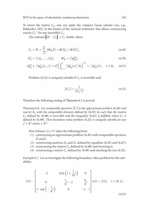
BVP in the space of absolutely continuous functions 183
To invert the matrix Ca, one can apply the compact Gauss scheme (see, e.g.,Bakhvalov [45]) in the frames of the rational arithmetic that allows constructingexactly C−1
a for any invertible Ca.
The estimate lX − Ca ≤ Cv, holds, where
Cv = Ψv +m∑
j=1
{Φ
jMX
jv + Φ
jvX
jN + Φ
jvX
jv}
, (6.49)
XjN =
{jx1N , . . . , jxnN
}, Φ
jM =
{jϕMkq
}, (6.50)
jϕMkq ≥∣∣ jϕakq
(t j−1
)∣∣ + tΔj
(∫ t j
t j−1
∣∣ jϕakq(s)
∣∣2ds)1/2
≥ ∣∣ jϕakq(t)∣∣, t ∈ E j . (6.51)
Problem (6.22) is uniquely solvable if Ca is invertible and
∥∥Cv
∥∥ <
1∥∥C−1
a
∥∥ . (6.52)
Therefore the following analog of Theorem 6.1 is proved.
Theorem 6.6. Let computable operators L, l in the approximate problem (6.26) andmatrix Xa with the computable elements defined by (6.32) be such that the matrixCa defined by (6.48) is invertible and the inequality (6.52) is fulfilled, where Cv isdefined by (6.49). Then boundary value problem (6.22) is uniquely solvable for anyf ∈ Ln and α ∈ Rn.
Now Scheme (1)–(7) takes the following form:(1) constructing an approximate problem (6.26) with computable operators
L and l;(2) constructing matrices Xa and Xv defined by equalities (6.32) and (6.47);(3) constructing the matrix Ca defined by (6.48) and inverting it;(4) constructing a matrix Cv defined by (6.49) and checking the test (6.52).
Example 6.7. Let us investigate the following boundary value problem for the solv-ability:
x(t)−
⎡
⎢⎢⎢⎢⎢⎢⎢⎢⎣
−2 2t ln(
1 +1
10t)
0
019t − 2
89t
t · exp(− 1
8t)
0 −2− t
⎤
⎥⎥⎥⎥⎥⎥⎥⎥⎦
x(t) = f (t), t ∈ [0, 1],
(6.53)
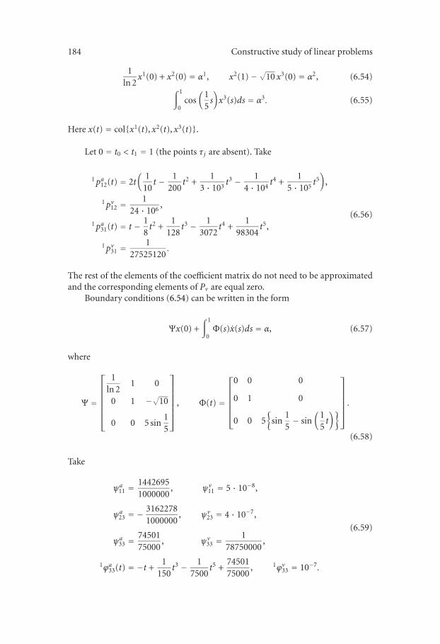
184 Constructive study of linear problems
1ln 2
x1(0) + x2(0) = α1, x2(1)−√10 x3(0) = α2, (6.54)∫ 1
0cos
(15s)x3(s)ds = α3. (6.55)
Here x(t) = col{x1(t), x2(t), x3(t)}.
Let 0 = t0 < t1 = 1 (the points τj are absent). Take
1pa12(t) = 2t(
110t − 1
200t2 +
13 · 103
t3 − 14 · 104
t4 +1
5 · 105t5)
,
1pv12 =1
24 · 106,
1pa31(t) = t − 18t2 +
1128
t3 − 13072
t4 +1
98304t5,
1pv31 =1
27525120.
(6.56)
The rest of the elements of the coefficient matrix do not need to be approximatedand the corresponding elements of Pv are equal zero.
Boundary conditions (6.54) can be written in the form
Ψx(0) +∫ 1
0Φ(s)x(s)ds = α, (6.57)
where
Ψ =
⎡
⎢⎢⎢⎢⎢⎢⎣
1ln 2
1 0
0 1 −√10
0 0 5 sin15
⎤
⎥⎥⎥⎥⎥⎥⎦
, Φ(t) =
⎡
⎢⎢⎢⎢⎢⎣
0 0 0
0 1 0
0 0 5{
sin15− sin
(15t)}
⎤
⎥⎥⎥⎥⎥⎦.
(6.58)
Take
ψa11 =14426951000000
, ψv11 = 5 · 10−8,
ψa23 = −31622781000000
, ψv23 = 4 · 10−7,
ψa33 =7450175000
, ψv33 =1
78750000,
1ϕa33(t) = −t +1
150t3 − 1
7500t5 +
7450175000
, 1ϕv33 = 10−7.
(6.59)
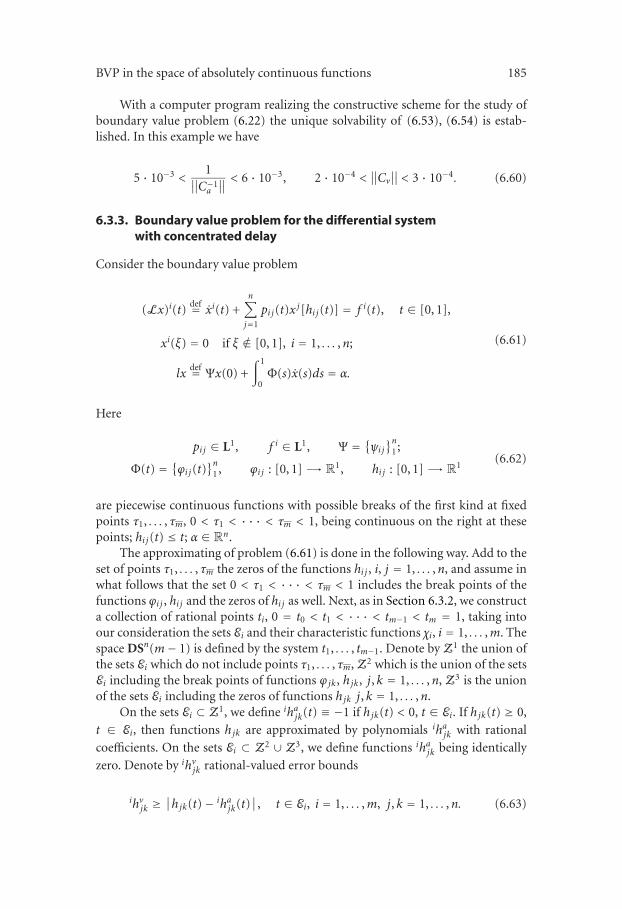
BVP in the space of absolutely continuous functions 185
With a computer program realizing the constructive scheme for the study ofboundary value problem (6.22) the unique solvability of (6.53), (6.54) is estab-lished. In this example we have
5 · 10−3 <1
∥∥C−1
a
∥∥ < 6 · 10−3, 2 · 10−4 <
∥∥Cv∥∥ < 3 · 10−4. (6.60)
6.3.3. Boundary value problem for the differential systemwith concentrated delay
Consider the boundary value problem
(Lx)i(t)def= xi(t) +
n∑
j=1
pi j(t)x j[hi j(t)] = f i(t), t ∈ [0, 1],
xi(ξ) = 0 if ξ �∈ [0, 1], i = 1, . . . ,n;
lxdef= Ψx(0) +
∫ 1
0Φ(s)x(s)ds = α.
(6.61)
Here
pi j ∈ L1, f i ∈ L1, Ψ = {ψij}n
1;
Φ(t) = {ϕij(t)}n
1 , ϕij : [0, 1] �→ R1, hi j : [0, 1] �→ R
1(6.62)
are piecewise continuous functions with possible breaks of the first kind at fixedpoints τ1, . . . , τm, 0 < τ1 < · · · < τm < 1, being continuous on the right at thesepoints; hi j(t) ≤ t; α ∈ Rn.
The approximating of problem (6.61) is done in the following way. Add to theset of points τ1, . . . , τm the zeros of the functions hi j , i, j = 1, . . . ,n, and assume inwhat follows that the set 0 < τ1 < · · · < τm < 1 includes the break points of thefunctions ϕij , hi j and the zeros of hi j as well. Next, as in Section 6.3.2, we constructa collection of rational points ti, 0 = t0 < t1 < · · · < tm−1 < tm = 1, taking intoour consideration the sets Ei and their characteristic functions χi, i = 1, . . . ,m. Thespace DSn(m− 1) is defined by the system t1, . . . , tm−1. Denote by Z1 the union ofthe sets Ei which do not include points τ1, . . . , τm, Z2 which is the union of the setsEi including the break points of functions ϕjk, hjk, j, k = 1, . . . ,n, Z3 is the unionof the sets Ei including the zeros of functions hjk j, k = 1, . . . ,n.
On the sets Ei ⊂ Z1, we define ihajk(t) ≡ −1 if hjk(t) < 0, t ∈ Ei. If hjk(t) ≥ 0,
t ∈ Ei, then functions hjk are approximated by polynomials ihajk with rational
coefficients. On the sets Ei ⊂ Z2 ∪ Z3, we define functions ihajk being identically
zero. Denote by ihvjk rational-valued error bounds
ihvjk ≥∣∣hjk(t)− ihajk(t)
∣∣, t ∈ Ei, i = 1, . . . ,m, j, k = 1, . . . ,n. (6.63)
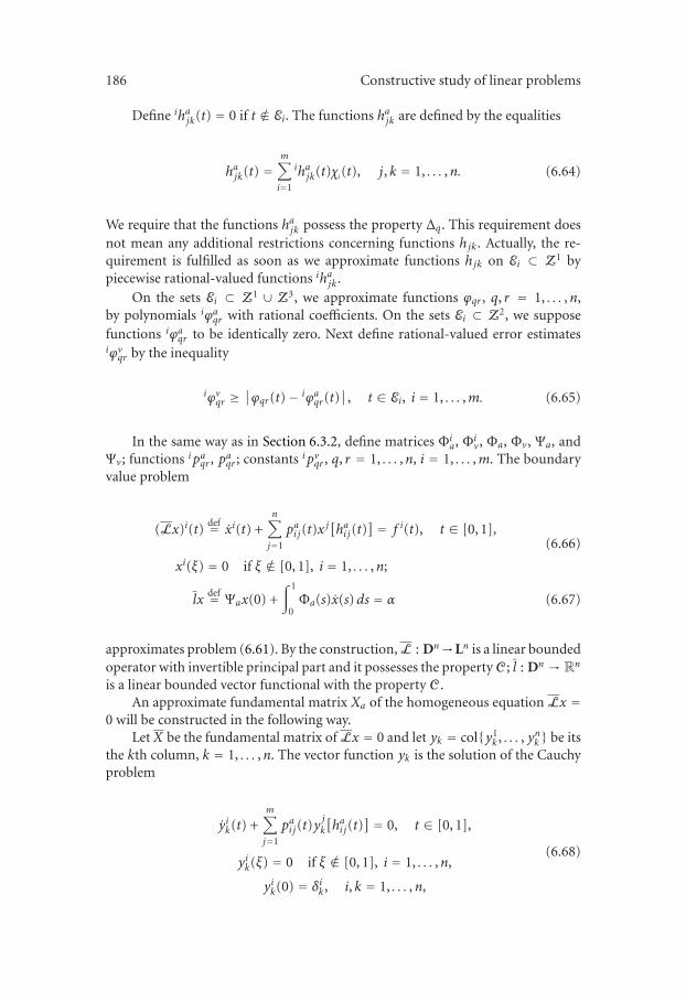
186 Constructive study of linear problems
Define ihajk(t) = 0 if t �∈ Ei. The functions hajk are defined by the equalities
hajk(t) =m∑
i=1
ihajk(t)χi(t), j, k = 1, . . . ,n. (6.64)
We require that the functions hajk possess the property Δq. This requirement doesnot mean any additional restrictions concerning functions hjk. Actually, the re-quirement is fulfilled as soon as we approximate functions hjk on Ei ⊂ Z1 bypiecewise rational-valued functions ihajk.
On the sets Ei ⊂ Z1 ∪ Z3, we approximate functions ϕqr , q, r = 1, . . . ,n,by polynomials iϕaqr with rational coefficients. On the sets Ei ⊂ Z2, we supposefunctions iϕaqr to be identically zero. Next define rational-valued error estimatesiϕvqr by the inequality
iϕvqr ≥∣∣ϕqr(t)− iϕaqr(t)
∣∣, t ∈ Ei, i = 1, . . . ,m. (6.65)
In the same way as in Section 6.3.2, define matrices Φia, Φi
v, Φa, Φv, Ψa, andΨv; functions i paqr , p
aqr ; constants i pvqr , q, r = 1, . . . ,n, i = 1, . . . ,m. The boundary
value problem
(Lx)i(t)def= xi(t) +
n∑
j=1
pai j(t)xj[hai j(t)
] = f i(t), t ∈ [0, 1],
xi(ξ) = 0 if ξ �∈ [0, 1], i = 1, . . . ,n;
(6.66)
lxdef= Ψax(0) +
∫ 1
0Φa(s)x(s)ds = α (6.67)
approximates problem (6.61). By the construction, L : Dn→Ln is a linear boundedoperator with invertible principal part and it possesses the property C; l : Dn → Rn
is a linear bounded vector functional with the property C.An approximate fundamental matrix Xa of the homogeneous equation Lx =
0 will be constructed in the following way.Let X be the fundamental matrix of Lx = 0 and let yk = col{y1
k , . . . , ynk} be itsthe kth column, k = 1, . . . ,n. The vector function yk is the solution of the Cauchyproblem
yik(t) +m∑
j=1
pai j(t)yjk
[hai j(t)
] = 0, t ∈ [0, 1],
yik(ξ) = 0 if ξ �∈ [0, 1], i = 1, . . . ,n,
yik(0) = δik, i, k = 1, . . . ,n,
(6.68)
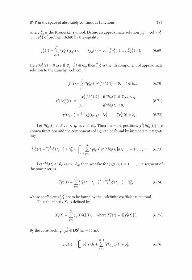
BVP in the space of absolutely continuous functions 187
where δik is the Kronecker symbol. Define an approximate solution yka = col{1yka ,. . . , nyka} of problem (6.68) by the equality
yka(t) =m∑
q=1
q yka(t)χq (t), q yka(·) = col{q
1 yka(·), . . . ,
qn yka(·)}. (6.69)
Here qyka(t) = 0 as t �∈ Eq; if t ∈ Eq, thenqi y
ka is the ith component of approximate
solution to the Cauchy problem
yi(t) +n∑
j=1
qpai j(t)yj[qhai j(t)
] = 0, t ∈ Eq, (6.70)
y j[qhai j(t)
] =⎧⎪⎨
⎪⎩
sjyka
[qhai j(t)
]if qhai j(t) ∈ Es, s < q,
0 if qhai j(t) < 0,(6.71)
yi(tq−1
) = q−1i y
ka
(tq−1
)+ iε
qk , 0
i yka(0) = δik. (6.72)
Let qhai j(t) ∈ Er , r < q, as t ∈ Eq. Then the superpositions y j[qhai j(t)] are
known functions and the components of qyka can be found by immediate integrat-ing:
qi y
ka(t) = q−1
i yka
(tq−1
)+ iε
qk −
∫ t
tq−1
n∑
j=1
qpai j(s)yj[qhai j(s)
]ds, i = 1, . . . ,n. (6.73)
Let qhai j(t) ∈ Eq as t ∈ Eq, then we take forqi y
ka(·), i = 1, . . . ,n, a segment of
the power series
qi y
ka(t) =
ν∑
j=1
ij cqk
(t − tq−1
) j+q−1i y
ka
(tq−1
)+ iε
qk , (6.74)
whose coefficients ij cqk are to be found by the indefinite coefficients method.
Thus the matrix Xa is defined by
Xa(t) =m∑
q=1
χq(t)Xqa (t), where X
qa (t) = {qi y ja(t)
}n1 . (6.75)
By the constructing, iyja ∈ DS1(m− 1) and
i yja(t) =
∫ t
0i y
ja(s)ds +
m−1∑
q=1
iεqχ[tq ,1] (t) + δij . (6.76)
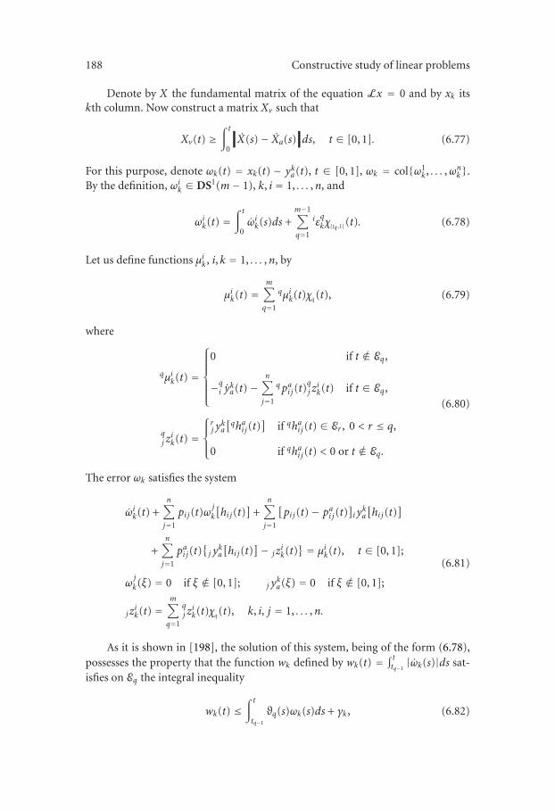
188 Constructive study of linear problems
Denote by X the fundamental matrix of the equation Lx = 0 and by xk itskth column. Now construct a matrix Xv such that
Xv(t) ≥∫ t
0X(s)− Xa(s) ds, t ∈ [0, 1]. (6.77)
For this purpose, denote ωk(t) = xk(t) − yka(t), t ∈ [0, 1], ωk = col{ω1k , . . . ,ωnk}.
By the definition, ωik ∈ DS1(m− 1), k, i = 1, . . . ,n, and
ωik(t) =∫ t
0ωik(s)ds +
m−1∑
q=1
iεqkχ[tq ,1] (t). (6.78)
Let us define functions μik, i, k = 1, . . . ,n, by
μik(t) =m∑
q=1
qμik(t)χq(t), (6.79)
where
qμik(t) =
⎧⎪⎪⎪⎪⎨
⎪⎪⎪⎪⎩
0 if t �∈ Eq,
−qi y
ka(t)−
n∑
j=1
q pai j(t)qj zik(t) if t ∈ Eq,
qj zik(t) =
⎧⎪⎨
⎪⎩
rj y
ka
[qhai j(t)
]if qhai j(t) ∈ Er , 0 < r ≤ q,
0 if qhai j(t) < 0 or t �∈ Eq.
(6.80)
The error ωk satisfies the system
ωik(t) +n∑
j=1
pi j(t)ωjk
[hi j(t)
]+
n∑
j=1
[pi j(t)− pai j(t)
]i yka
[hi j(t)
]
+n∑
j=1
pai j(t){j y
ka
[hi j(t)
]− j zik(t)
} = μik(t), t ∈ [0, 1];
ωjk(ξ) = 0 if ξ �∈ [0, 1]; j y
ka(ξ) = 0 if ξ �∈ [0, 1];
j zik(t) =
m∑
q=1
qj zik(t)χq(t), k, i, j = 1, . . . ,n.
(6.81)
As it is shown in [198], the solution of this system, being of the form (6.78),possesses the property that the function wk defined by wk(t) = ∫ ttq−1
|ωk(s)|ds sat-isfies on Eq the integral inequality
wk(t) ≤∫ t
tq−1
ϑq(s)ωk(s)ds + γk, (6.82)
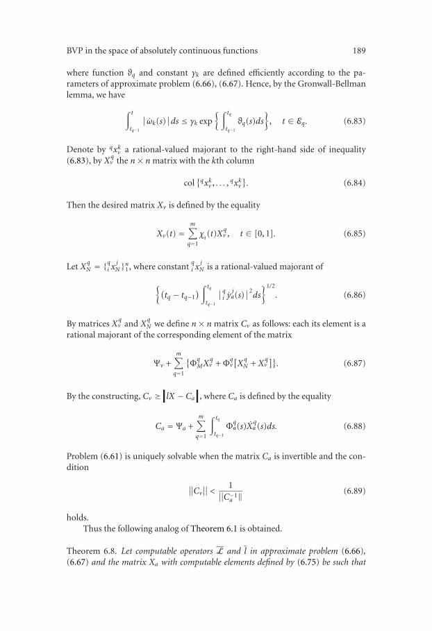
BVP in the space of absolutely continuous functions 189
where function ϑq and constant γk are defined efficiently according to the pa-rameters of approximate problem (6.66), (6.67). Hence, by the Gronwall-Bellmanlemma, we have
∫ t
tq−1
∣∣ωk(s)
∣∣ds ≤ γk exp
{∫ tq
tq−1
ϑq(s)ds}
, t ∈ Eq. (6.83)
Denote by qxkv a rational-valued majorant to the right-hand side of inequality(6.83), by X
qv the n× n matrix with the kth column
col{qxkv , . . . , qxkv
}. (6.84)
Then the desired matrix Xv is defined by the equality
Xv(t) =m∑
q=1
χq(t)Xqv , t ∈ [0, 1]. (6.85)
Let XqN = {qi x jN}n1, where constant
qi x
jN is a rational-valued majorant of
{(tq − tq−1
)∫ tq
tq−1
∣∣qi y
ja(s)
∣∣2ds}1/2
. (6.86)
By matrices Xqv and X
qN we define n× n matrix Cv as follows: each its element is a
rational majorant of the corresponding element of the matrix
Ψv +m∑
q=1
{ΦqMX
qv + Φ
qv[XqN + X
qv]}. (6.87)
By the constructing, Cv ≥ lX − Ca , where Ca is defined by the equality
Ca = Ψa +m∑
q=1
∫ tq
tq−1
Φqa(s)X
qa (s)ds. (6.88)
Problem (6.61) is uniquely solvable when the matrix Ca is invertible and the con-dition
∥∥Cv
∥∥ <
1∥∥C−1
a ‖(6.89)
holds.Thus the following analog of Theorem 6.1 is obtained.
Theorem 6.8. Let computable operators L and l in approximate problem (6.66),(6.67) and the matrix Xa with computable elements defined by (6.75) be such that
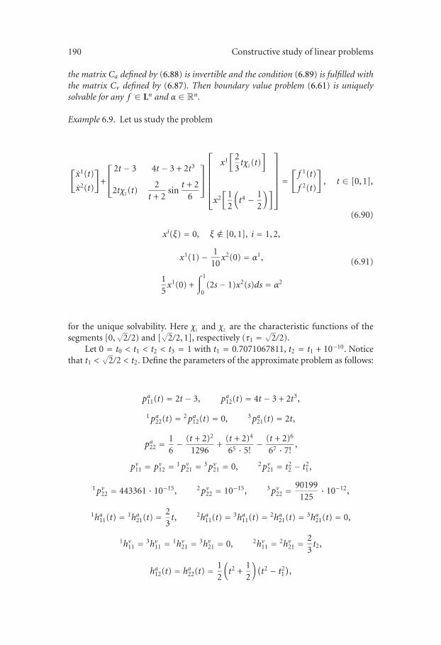
190 Constructive study of linear problems
the matrix Ca defined by (6.88) is invertible and the condition (6.89) is fulfilled withthe matrix Cv defined by (6.87). Then boundary value problem (6.61) is uniquelysolvable for any f ∈ Ln and α ∈ Rn.
Example 6.9. Let us study the problem
[x1(t)
x2(t)
]
+
⎡
⎢⎣
2t − 3 4t − 3 + 2t3
2tχ2 (t)2
t + 2sin
t + 26
⎤
⎥⎦
⎡
⎢⎢⎢⎢⎢⎢⎣
x1[
23tχ1 (t)
]
x2[
12
(t4 − 1
2
)]
⎤
⎥⎥⎥⎥⎥⎥⎦
=[f 1(t)
f 2(t)
]
, t ∈ [0, 1],
(6.90)
xi(ξ) = 0, ξ �∈ [0, 1], i = 1, 2,
x1(1)− 110x2(0) = α1,
15x1(0) +
∫ 1
0(2s− 1)x2(s)ds = α2
(6.91)
for the unique solvability. Here χ1 and χ2 are the characteristic functions of thesegments [0,
√2/2) and [
√2/2, 1], respectively (τ1 =
√2/2).
Let 0 = t0 < t1 < t2 < t3 = 1 with t1 = 0.7071067811, t2 = t1 + 10−10. Noticethat t1 <
√2/2 < t2. Define the parameters of the approximate problem as follows:
pa11(t) = 2t − 3, pa12(t) = 4t − 3 + 2t3,
1pa22(t) = 2pa12(t) = 0, 3pa21(t) = 2t,
pa22 =16− (t + 2)2
1296+
(t + 2)4
65 · 5!− (t + 2)6
67 · 7!,
pv11 = pv12 = 1pv21 = 3pv21 = 0, 2pv21 = t22 − t21,
1pv22 = 443361 · 10−15, 2pv22 = 10−15, 3pv22 =90199
125· 10−12,
1ha11(t) = 1ha21(t) = 23t, 2ha11(t) = 3ha11(t) = 2ha21(t) = 3ha21(t) = 0,
1hv11 = 3hv11 = 1hv21 = 3hv21 = 0, 2hv11 = 2hv21 =23t2,
ha12(t) = ha22(t) = 12
(t2 +
12
)(t2 − t21
),
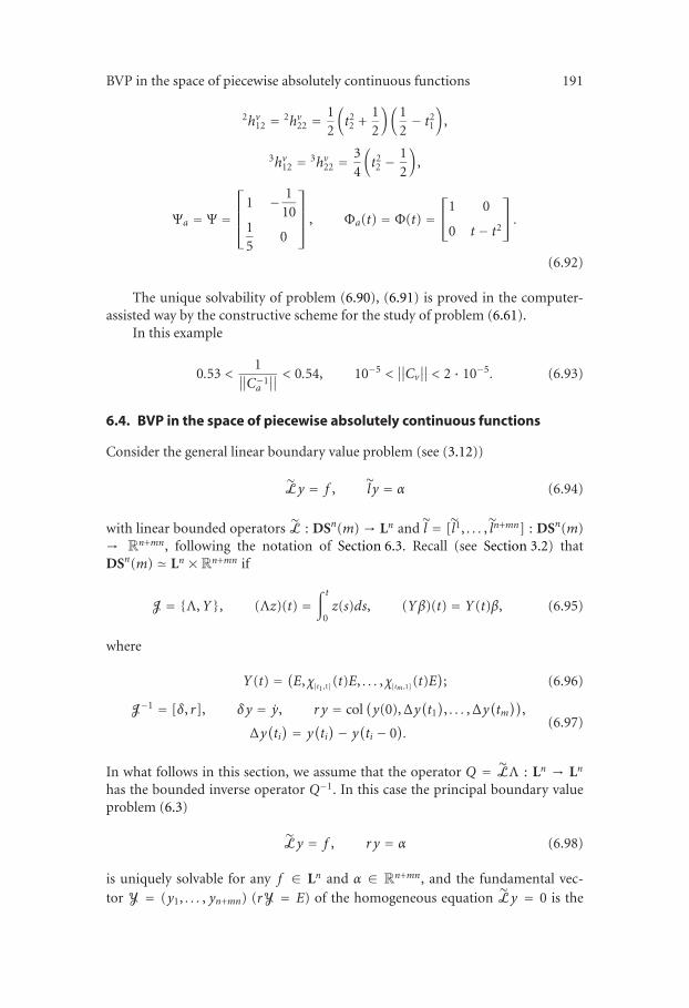
BVP in the space of piecewise absolutely continuous functions 191
2hv12 = 2hv22 =12
(t22 +
12
)(12− t21
),
3hv12 = 3hv22 =34
(t22 −
12
),
Ψa = Ψ =
⎡
⎢⎢⎣
1 − 110
15
0
⎤
⎥⎥⎦ , Φa(t) = Φ(t) =
⎡
⎣1 0
0 t − t2
⎤
⎦ .
(6.92)
The unique solvability of problem (6.90), (6.91) is proved in the computer-assisted way by the constructive scheme for the study of problem (6.61).
In this example
0.53 <1
∥∥C−1
a
∥∥ < 0.54, 10−5 <
∥∥Cv
∥∥ < 2 · 10−5. (6.93)
6.4. BVP in the space of piecewise absolutely continuous functions
Consider the general linear boundary value problem (see (3.12))
Ly = f , l y = α (6.94)
with linear bounded operators L : DSn(m) → Ln and l = [l1, . . . , ln+mn] : DSn(m)→ Rn+mn, following the notation of Section 6.3. Recall (see Section 3.2) thatDSn(m) � Ln ×Rn+mn if
J = {Λ,Y}, (Λz)(t) =∫ t
0z(s)ds, (Yβ)(t) = Y(t)β, (6.95)
where
Y(t) = (E, χ[t1,1] (t)E, . . . , χ[tm ,1] (t)E); (6.96)
J−1 = [δ, r], δy = y, r y = col(y(0),Δy
(t1), . . . ,Δy
(tm))
,
Δy(ti) = y
(ti)− y
(ti − 0
).
(6.97)
In what follows in this section, we assume that the operator Q = LΛ : Ln → Ln
has the bounded inverse operator Q−1. In this case the principal boundary valueproblem (6.3)
Ly = f , r y = α (6.98)
is uniquely solvable for any f ∈ Ln and α ∈ Rn+mn, and the fundamental vec-tor Y = (y1, . . . , yn+mn) (rY = E) of the homogeneous equation Ly = 0 is the
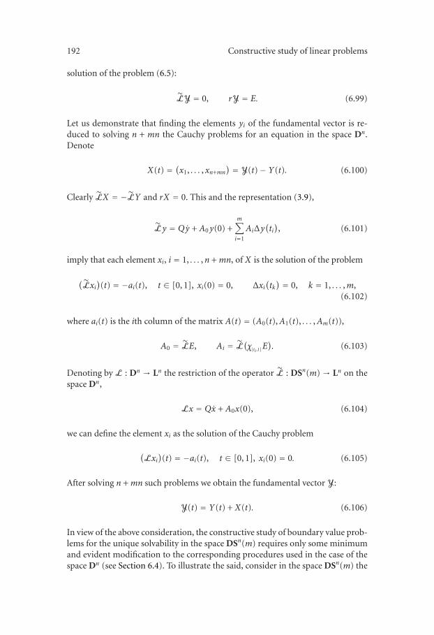
192 Constructive study of linear problems
solution of the problem (6.5):
LY = 0, rY = E. (6.99)
Let us demonstrate that finding the elements yi of the fundamental vector is re-duced to solving n + mn the Cauchy problems for an equation in the space Dn.Denote
X(t) = (x1, . . . , xn+mn) = Y(t)− Y(t). (6.100)
Clearly LX = −LY and rX = 0. This and the representation (3.9),
Ly = Qy +A0y(0) +m∑
i=1
AiΔy(ti), (6.101)
imply that each element xi, i = 1, . . . ,n +mn, of X is the solution of the problem
(Lxi
)(t) = −ai(t), t ∈ [0, 1], xi(0) = 0, Δxi
(tk) = 0, k = 1, . . . ,m,
(6.102)
where ai(t) is the ith column of the matrix A(t) = (A0(t),A1(t), . . . ,Am(t)),
A0 = LE, Ai = L(χ[ti ,1]E
). (6.103)
Denoting by L : Dn → Ln the restriction of the operator L : DSn(m) → Ln on thespace Dn,
Lx = Qx + A0x(0), (6.104)
we can define the element xi as the solution of the Cauchy problem
(Lxi
)(t) = −ai(t), t ∈ [0, 1], xi(0) = 0. (6.105)
After solving n +mn such problems we obtain the fundamental vector Y:
Y(t) = Y(t) + X(t). (6.106)
In view of the above consideration, the constructive study of boundary value prob-lems for the unique solvability in the space DSn(m) requires only some minimumand evident modification to the corresponding procedures used in the case of thespace Dn (see Section 6.4). To illustrate the said, consider in the space DSn(m) the
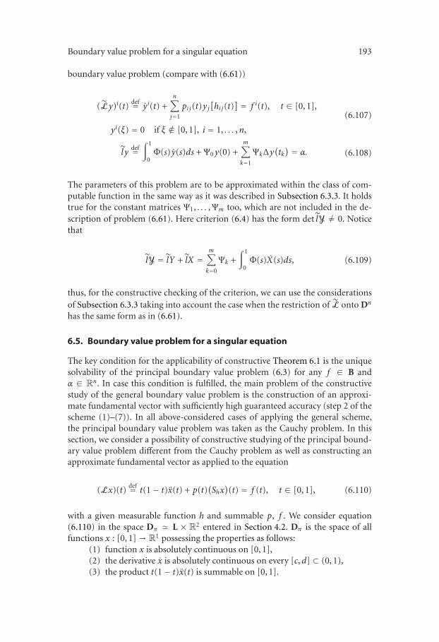
Boundary value problem for a singular equation 193
boundary value problem (compare with (6.61))
(Ly)i(t)def= yi(t) +
n∑
j=1
pi j(t)yj[hi j(t)
] = f i(t), t ∈ [0, 1],
yi(ξ) = 0 if ξ �∈ [0, 1], i = 1, . . . ,n,
(6.107)
l ydef=∫ 1
0Φ(s) y(s)ds + Ψ0y(0) +
m∑
k=1
ΨkΔy(tk) = α. (6.108)
The parameters of this problem are to be approximated within the class of com-putable function in the same way as it was described in Subsection 6.3.3. It holdstrue for the constant matrices Ψ1, . . . ,Ψm too, which are not included in the de-scription of problem (6.61). Here criterion (6.4) has the form det lY �= 0. Noticethat
lY = lY + lX =m∑
k=0
Ψk +∫ 1
0Φ(s)X(s)ds, (6.109)
thus, for the constructive checking of the criterion, we can use the considerationsof Subsection 6.3.3 taking into account the case when the restriction of L onto Dn
has the same form as in (6.61).
6.5. Boundary value problem for a singular equation
The key condition for the applicability of constructive Theorem 6.1 is the uniquesolvability of the principal boundary value problem (6.3) for any f ∈ B andα ∈ Rn. In case this condition is fulfilled, the main problem of the constructivestudy of the general boundary value problem is the construction of an approxi-mate fundamental vector with sufficiently high guaranteed accuracy (step 2 of thescheme (1)–(7)). In all above-considered cases of applying the general scheme,the principal boundary value problem was taken as the Cauchy problem. In thissection, we consider a possibility of constructive studying of the principal bound-ary value problem different from the Cauchy problem as well as constructing anapproximate fundamental vector as applied to the equation
(Lx)(t)def= t(1− t)x(t) + p(t)
(Shx)(t) = f (t), t ∈ [0, 1], (6.110)
with a given measurable function h and summable p, f . We consider equation(6.110) in the space Dπ � L × R2 entered in Section 4.2. Dπ is the space of allfunctions x : [0, 1] → R1 possessing the properties as follows:
(1) function x is absolutely continuous on [0, 1],(2) the derivative x is absolutely continuous on every [c,d] ⊂ (0, 1),(3) the product t(1− t)x(t) is summable on [0, 1].
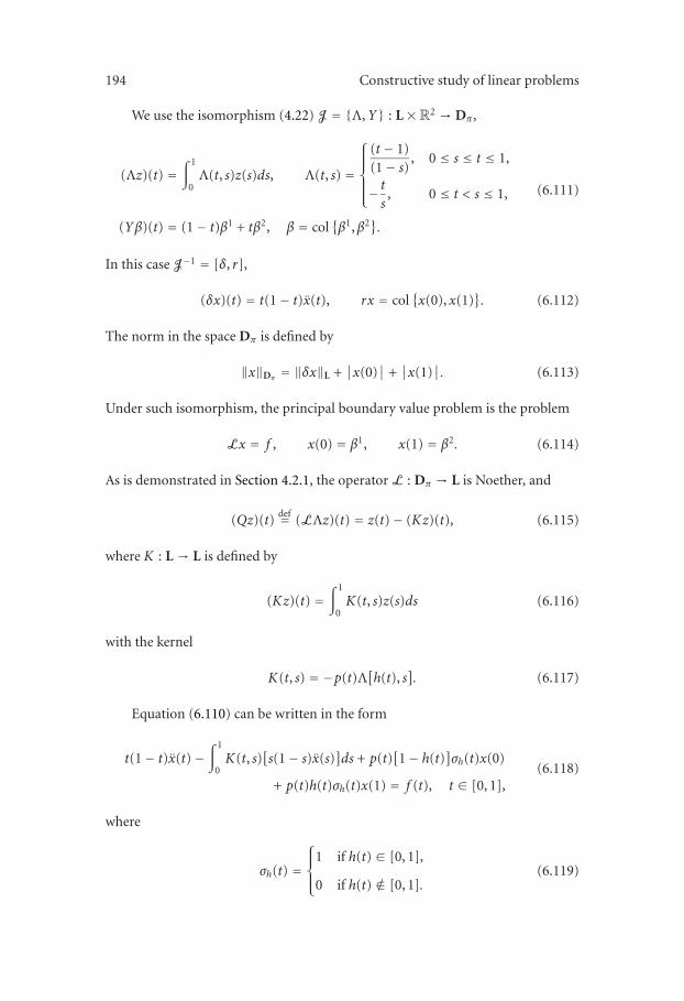
194 Constructive study of linear problems
We use the isomorphism (4.22) J = {Λ,Y} : L×R2 → Dπ ,
(Λz)(t) =∫ 1
0Λ(t, s)z(s)ds, Λ(t, s) =
⎧⎪⎪⎪⎨
⎪⎪⎪⎩
(t − 1)(1− s) , 0 ≤ s ≤ t ≤ 1,
− ts, 0 ≤ t < s ≤ 1,
(Yβ)(t) = (1− t)β1 + tβ2, β = col{β1,β2}.
(6.111)
In this case J−1 = [δ, r],
(δx)(t) = t(1− t)x(t), rx = col{x(0), x(1)
}. (6.112)
The norm in the space Dπ is defined by
‖x‖Dπ = ‖δx‖L +∣∣x(0)
∣∣ +
∣∣x(1)
∣∣. (6.113)
Under such isomorphism, the principal boundary value problem is the problem
Lx = f , x(0) = β1, x(1) = β2. (6.114)
As is demonstrated in Section 4.2.1, the operator L : Dπ → L is Noether, and
(Qz)(t)def= (LΛz)(t) = z(t)− (Kz)(t), (6.115)
where K : L → L is defined by
(Kz)(t) =∫ 1
0K(t, s)z(s)ds (6.116)
with the kernel
K(t, s) = −p(t)Λ[h(t), s
]. (6.117)
Equation (6.110) can be written in the form
t(1− t)x(t)−∫ 1
0K(t, s)
[s(1− s)x(s)
]ds + p(t)
[1− h(t)
]σh(t)x(0)
+ p(t)h(t)σh(t)x(1) = f (t), t ∈ [0, 1],(6.118)
where
σh(t) =⎧⎪⎨
⎪⎩
1 if h(t) ∈ [0, 1],
0 if h(t) �∈ [0, 1].(6.119)
Boundary value problem for a singular equation 195
Here and in what follows the function Λ(t, s) is equal to zero outside the square[0, 1] × [0, 1]. The operator K : L → L is compact (Theorem B.1) and, hence,Q : L → L is a canonical Fredholm operator. The invertibility of this operator isa criterion of the unique solvability of principal boundary value problem (6.114)for any f ∈ L1, β1,β2 ∈ R (Theorem 1.16). The standard conditions for the in-vertibility of Q of the form ‖K‖L→L < 1 or ρ(K) < 1 can be too rough to be usefulfor the study of concrete boundary value problems. Our constructive approachenables us to extend essentially the possibilities for establishing the invertibility ofI − K .
Fix ε ∈ (0, 1). Let
K(t, s) =N∑
i=1
ui(t)vi(s) (6.120)
be a degenerate kernel with measurable essentially bounded functions vi and sum-mable ui such that
ess sups∈[0,1]
∫ 1
0
∣∣K(t, s)− K(t, s)∣∣dt ≤ ε. (6.121)
Next, let the N ×N matrix
E − A, A− {ai j}, ai j =∫ 1
0vi(t)uj(t)dt, i, j = 1, . . . ,N , (6.122)
be invertible.Denote by bi j the elements of the matrix B = (E − A)−1 and
H(t, s) =N∑
j=1
N∑
i=1
ui(t)bi jv j(s). (6.123)
The function H(t, s) is the resolvent kernel of K(t, s): for each f ∈ L, the uniquesolution of the equation
z(t)−∫ 1
0K(t, s)z(s)ds = f (t), t ∈ [0, 1], (6.124)
is the function
z(t) = f (t) +∫ 1
0H(t, s) f (s)ds. (6.125)
Let d be such that
ess sups
∫ 1
0
∣∣H(t, s)
∣∣dt ≤ d. (6.126)
196 Constructive study of linear problems
If the inequality
ε <1
1 + d(6.127)
holds, then due to the theorem on invertible operator (see, e.g., [100, Theorem3.6.3]) the operator I − K has the bounded inverse and the principal boundaryvalue problem (6.117) is uniquely solvable for any f ∈ L, β1,β2 ∈ R. Notice thatinequality (6.127) can be checked with the computing experiment if the functionsui, vi, i = 1, . . . ,N , are computable.
Assuming condition (6.127) is fulfilled, consider the question on constructingan approximation to fundamental vector X = (x1, x2) of the equation Lx = 0(LX = 0, rX = E) with a guaranteed error bound. The element x1 is the solutionof the problem
Lx = 0, x(0) = 1, x(1) = 0 (6.128)
and has the representation
x1(t) = (Λz1)(t) + (1− t), (6.129)
where z1(t) is the solution of the equation
z(t)−∫ 1
0K(t, s)z(s)ds = −p(t)
[1− h(t)
]σh(t), t ∈ [0, 1], (6.130)
σh(t) =⎧⎪⎨
⎪⎩
1 if h(t) ∈ [0, 1],
0 if h(t) �∈ [0, 1].(6.131)
For x2 we have the problem
Lx = 0, x(0) = 0, x(1) = 1 (6.132)
and, therefore,
x2(t) = (Λz2)(t) + t, (6.133)
where z2(t) is the solution of the equation
z(t)−∫ 1
0K(t, s)z(s)ds = −p(t)h(t)σh(t), t ∈ [0, 1]. (6.134)
Boundary value problem for a singular equation 197
Denoting by z1 (z2) the solution of (6.130) (of (6.134)), where the kernel K(t, s) isreplaced by K(t, s), we obtain due to the known estimate (see, e.g., [100, Theorem3.6.3]), taking place under the conditions of the invertible operator theorem, thefollowing inequalities:
∫ 1
0
∣∣z1(t)− z1(t)
∣∣dt ≤ ε
(1 + d)2
1− ε(1 + d)
∫ 1
0
∣∣p(t)
∣∣(1− h(t)
)σh(t)dt
def= ε1,
∫ 1
0
∣∣z2(t)− z2(t)
∣∣dt ≤ ε
(1 + d)2
1− ε(1 + d)
∫ 1
0
∣∣p(t)
∣∣h(t)σh(t)dt
def= ε2.
(6.135)
These estimates allow us to obtain a guaranteed error bound for the approxi-mate fundamental vector (x1, x2).
Now consider the boundary value problem for equation (6.110) with the gen-eral linear boundary conditions
lix = αi, i = 1, 2. (6.136)
The linear bounded functional li : Dπ → R has the representation
lix =∫ 1
0ϕi(t)t(1− t)x(t)dt + ψi1x(0) + ψi2x(1), (6.137)
where function ϕi is measurable and essentially bounded on [0, 1], ψi,1,ψi,2 =const.
A criterion of the unique solvability of (6.110), (6.136) is the invertibility ofthe matrix {lix j}, i, j = 1, 2. Estimates (6.135) together with the possibility ofconstructing functions z1 and z2 allow us to check efficiently this criterion. Indeed,the presentation (6.137) implies
lix j =∫ 1
0ϕi(t)zj(t)dt + ψij . (6.138)
Denote
θ = {ϑi j}, ϑi j =∫ 1
0ϕi(t)z j(t)dt + ψij , i, j = 1, 2. (6.139)
The estimates (6.135) imply
∣∣ϑi j − lix j∣∣ ≤ εj · qi, (6.140)
where qi ≥ ess supt∈[0,1] |ϕi(t)|.If the matrix θ is invertible and
max{q1, q2
}(ε1 + ε2
)<
1∥∥θ−1
∥∥ , (6.141)
198 Constructive study of linear problems
then the matrix {lix j} of problem (6.110), (6.136) is invertible too, that is, thisproblem is uniquely solvable.
Notice that the computer experiment realizing the above scheme allows usto recognize the unique solvability for any uniquely solvable problem such thatits kernel K(t, s) can be approximated with such an accuracy as we wish by thekernels K(t, s) with computable functions ui, vi and the functions ϕ1, ϕ2 can beapproximated by computable functions with any required accuracy in the uniformmetric.
Example 6.10. Consider problem (6.110), (6.136) with the functional li defined by(6.137) and p(t) ≡ 10,
h(t) =
⎧⎪⎪⎪⎪⎪⎪⎪⎪⎪⎪⎪⎪⎪⎪⎪⎪⎪⎪⎪⎪⎪⎪⎪⎪⎪⎪⎪⎪⎪⎪⎨
⎪⎪⎪⎪⎪⎪⎪⎪⎪⎪⎪⎪⎪⎪⎪⎪⎪⎪⎪⎪⎪⎪⎪⎪⎪⎪⎪⎪⎪⎪⎩
t − 14
, t ∈ [0, 0.25), ϕ1(t) = χ[0.26,0.49]∪[0.51,0.74] (t)
1008t − 3, t ∈ [0.25, 0.26), ϕ1(t) = χ[0.26,0.49]∪[0.51,0.74] (t),
14
, t ∈ [0.26, 0.49), ϕ2(t) = χ[0.51,0.74] (t)
25t − 12, t ∈ [0.49, 0.51), ϕ2(t) = χ[0.51,0.74] (t),
34
, t ∈ [0.51, 0.74), ψ11 = 6, ψ12 = −0.6,
1008t − 17
2, t ∈ [0.74, 0.75), ψ11 = 6, ψ12 = −0.6,
t +14
, t ∈ [0.75, 1], ψ21 = −4.5, ψ22 = 13.6.
(6.142)
We will follow the above scheme of the study. Define the kernel K(t, s) by (6.120),where
u1(t) = −10χ[1/4,1/2] (t), u2(t) = −10χ[1/2,3/4] (t),
v1(s) = − 34(1− s)χ[0,1/4] (s)−
14sχ[1/4,1] (s),
v2(s) = − 14(1− s)χ[0,3/4] (s)−
34sχ[3/4,1] (s).
(6.143)
Here ε, the error bound of the approximation to K(t, s) (6.114) defined by (6.121),is no greater than 0.2. The resolvent kernel H(t, s) is defined by (6.123), whereb11 = b22 = 1.123, b12 = b21 = −1.554, and d < 1.1. Next
z1(t) = −10[1− h(t)]χ[1/4,3/4] (t) + 1.7χ[1/4,1/2] (t) + 26.7χ[1/2,3/4] (t),
z2(t) = − 10h(t)χ[1/4,3/4] (t) + 16.6χ[1/4,1/2] (t)− 8.4χ[1/2,3/4] (t),(6.144)
The Cauchy matrix and a posteriori error bounds 199
and ε1 + ε2 ≤ 7.604 (see (6.135)). The matrix θ (6.139) is defined by
θ =(
10.232 −1.0141.066 9.943
)
. (6.145)
Thus
θ−1 = 110.232 · 9.943 + 1.066 · 1.014
(9.943 1.014−1.066 10.232
)
, (6.146)
and ‖θ−1‖ < 0.113, 1/‖θ−1‖ > 8.5.Since in this example q1 = q2 = 1, inequality (6.141)
ε1 + ε2 ≤ 7.604 < 8.5 <1
∥∥θ−1∥∥ (6.147)
holds and, consequently, the boundary value problem under consideration isuniquely solvable for any f ∈ L and α1,α2 ∈ R.
In conclusion it may be said that in this example, ‖K‖L→L > 3.
6.6. The Cauchy matrix and a posteriori error bounds
Efficiency in realizing the scheme (1)–(7) depends essentially on fineness of guar-anteed error bounds for the approximate fundamental vector. For a posteriorierror bounds obtained by computing (or estimating) the defect, this fineness isdefined either by the accuracy in solving the corresponding operator (most of-ten, integral) inequality for the error or by the exactness of the estimate for thenorm of the Green operator G0 to the principal boundary value problem (6.3)(see Theorem 6.1).
Consider the possibility of constructing the mentioned a posteriori errorbounds as applied to the equation
Lx = f , (6.148)
with linear bounded operator L : Dn → Ln (in this section Ln = Ln[0,T], Dn =Dn[0,T], (Λz)(t) = ∫ t0 z(s)ds, (Yα)(t) = Eα, δx = x, rx = x(0)) having the princi-pal part Q : Ln → Ln of the form
(Qz)(t) = z(t)−∫ t
0K(t, s)z(s)ds, (6.149)
where the elements ki j(t, s) of the kernel K(t, s) are measurable in the triangle0 ≤ s ≤ t ≤ T and satisfy the inequalities
∣∣ki j(t, s)∣∣ ≤ μ(t), μ ∈ L1, i, j = 1, . . . ,n. (6.150)
200 Constructive study of linear problems
Recall that in this event equation (6.148) covers as the special cases the equationswith concentrated or distributed delay (see Section 2.2). The operator Q has thebounded inverse Q−1:
(Q−1z
)(t) = z(t) +
∫ t
0H(t, s)z(s)ds, (6.151)
where H(t, s) is the resolvent kernel for K(t, s). The principal boundary valueproblem (here the Cauchy problem)
Lx = f , x(0) = α (6.152)
is uniquely solvable for any f ∈ Ln and α ∈ Rn. Problem (6.5) for the fundamentalvector X = (x1, . . . , xn) has the form
LX = 0, X(0) = E. (6.153)
Thus the column xi is the solution of the problem
Lx = 0, x(0) = ei, (6.154)
where ei is the ith column of the identity n × n matrix. The solution x of theproblem (6.152) has the form
x(t) = X(t)α +∫ t
0C(t, s) f (s)ds, (6.155)
where C(t, s) is the Cauchy matrix possessing the following properties (see Subsec-tion 2.2.3):
C′t (t, s) = H(t, s), 0 ≤ s ≤ t ≤ T , (6.156)
C′t (t, s) =∫ t
sC′t (t, τ)K(τ, s)dτ + K(t, s), 0 ≤ s ≤ t ≤ T , (6.157)
C(t, s) = E +∫ t
sC′τ(τ, s)dτ, 0 ≤ s ≤ t ≤ T. (6.158)
Let Xa = (xa1, . . . , xan) be an approximation of the fundamental vector:
Lxai = Δi, xai (0) = ei. (6.159)
A simple way of constructing the estimate of the error yi = (xi − xai ) is as follows.For zi = yi we have
zi(t) =∫ t
0K(t, s)zi(s)ds + Δi(t), (6.160)
The Cauchy matrix and a posteriori error bounds 201
that implies
∣∣zi(t)
∣∣ ≤
∫ t
0
∥∥K(t, s)
∥∥ · ∣∣zi(s)
∣∣ds +
∣∣Δi(t)
∣∣, (6.161)
and, by the theorem on integral inequality, we obtain
∣∣zi(t)
∣∣ ≤ m(t)
∫ t
0exp
(∫ t
sm(τ)dτ
)∣∣Δi(s)
∣∣ds +
∣∣Δi(t)
∣∣, (6.162)
where m(t) = ‖{μi j(t)}‖, μi j(t) = μ(t), i, j = 1 . . . ,n. Hence
∣∣yi(t)
∣∣ ≤
∫ t
0m(τ) exp
(∫ τ
0m(ξ)dξ
)∫ τ
0
∣∣Δi(s)
∣∣ds dτ +
∫ t
0
∣∣Δi(s)
∣∣ds, t ∈ [0,T].
(6.163)
The presence of exponential factor in the right-hand side of (6.163) indicatesthat even for modest values n and T (say, n = 10, T = 5) estimate (6.163) can behighly overstated with respect to actual values of error.
Consider now an alternate way of constructing an error bound. This way isbased on constructing an approximation C(t, s) of the Cauchy matrix C(t, s) suchthat the norm ‖C − C‖Ln→Ln∞ is no greater than a given εC ; here C, C : Ln → Ln∞are linear integral Volterra operators with kernels C(t, s) and C(t, s), respectively.In this event, for |yi(t)| we have the estimate
∣∣yi(t)
∣∣ ≤
∫ t
0
∥∥C(t, s)
∥∥ · ∣∣Δi(s)
∣∣ds + εC ·
∫ T
0
∣∣Δi(s)
∣∣ds, t ∈ [0,T]. (6.164)
This estimate is essentially more accurate than (6.163) if it is possible to constructa sufficiently good approximation C(t, s). We will describe an efficiently realizableway of constructing such an approximation under the condition that the kernelK(t, s) admits a piecewise constant approximation being as accurate as we wish.This way can be extended to more wide classes of kernels.
Split the segment [0,T] on N + 1 equal parts by the points 0 = t0 < t1 < · · · <tN+1 = T and denote ti+1 − ti = �.
Next, on every square
�i jdef= (
ti, ti+1)× (t j−1, t j
), i = 1, . . . ,N , j = 1, . . . , i, (6.165)
we replace the matrix K(t, s) by the constant matrix Kij and assume constant n×nmatrices ΔKij to be known such that
∣∣K(t, s)− Kij∣∣ ≤ ΔKij , (t, s) ∈ �i j , i = 1, . . . ,N , j = 1, . . . , i. (6.166)
202 Constructive study of linear problems
Here the symbol |A| for a matrix A = {ai j}means the matrix {|ai j|}. Denote
ηi(t) =⎧⎨
⎩
1, t ∈ [ti, ti+1],
0, t �∈ [ti, ti+1],
i = 0, 1, . . . ,N.
Γ =
⎛
⎜⎜⎜⎜⎜⎜⎜⎜⎜⎝
E 0 0 · · · 0
−�K22 E 0 · · · 0
−�K32 −�K33 E · · · 0
......
.... . .
...
−�KN2 −�KN3 −�KN4 . . . E
⎞
⎟⎟⎟⎟⎟⎟⎟⎟⎟⎠
, Γ−1 = {Bij}
, i, j = 1, . . . ,N ,
K(t, s) = Kij , (t, s) ∈ �i j , i = 1, . . . ,N ; j = 1, . . . , i.(6.167)
The resolvent kernel H(t, s) for K(t, s) can be found in the explicit form (see, e.g.,Maksimov et al. [151]):
H(t, s) =N∑
i=1
ηi(t)i∑
k=1
Ξikηk−1(s), (6.168)
where
Ξik =i∑
j=kBi jKjk. (6.169)
Define the matrices C′t (t, s) and C(t, s) by the equalities
C′t (t, s)def= H(t, s), C(t, s) = E +
∫ t
sH(τ, s)dτ. (6.170)
Also define the linear operators K , K , H ,ΔK : Ln → Ln as integral operators withthe kernels K(t, s) K(t, s), H(t, s) and [K(t, s)− K(t, s)], respectively.
The inequality
qdef= ∥∥ΔK(I + H)
∥∥Ln→Ln < 1 (6.171)
allows us, applying the theorem on invertible operator, to obtain the estimate
‖C − C‖Ln→Ln∞ ≤ ‖H − H‖Ln→Ln ≤ q
1− q‖I + H‖Ln→Ln . (6.172)
Thus under (6.171) we can replace the constant εC in (6.164) by the right-hand sideof (6.172). Notice that constants q and ‖I + H‖Ln→Ln can be calculated efficientlywith computer.
Other applications of the constructive approach 203
Example 6.11. Consider the Cauchy problem
x(t)− p(t)xh(t) = 1, t ∈ [0, 5],
x(0) = 0,(6.173)
where p(t) = η1(t)− 2η2(t)− 2η3(t) + 3η4(t)− η6(t)− η7(t) + 4η8(t) + 4η9(t),
h(t) = 0.4η1(t) + 0.9η2(t) + 0.1η3(t) + 0.7η4(t)
− η5(t) + 0.2η6(t) + η7(t) + 2η8(t) + 3η9(t),
ηi(t) = χ[0.5i;0.5(i+1)] (t), i = 1, . . . , 9.
(6.174)
Let xa(t) be an approximate solution of (6.173) giving the defect Δ(t) with theestimate
∣∣Δ(t)
∣∣ ≤ ε, t ∈ [0, 5]. (6.175)
Here a posteriori estimate (6.163) has the form
∣∣xa(t)− x(t)
∣∣ ≤ 5
9
(e9 − 1
)ε, t ∈ [0, 5]. (6.176)
The estimate obtained with (6.172) is as follows:
∣∣xa(t)− x(t)
∣∣ ≤ 165ε, t ∈ [0, 5] (6.177)
(in this case the estimate ‖H‖L1→L1 ≤ 10 is used, it is obtained in the way as it wasdescribed above).
6.7. Other applications of the constructive approach
Considering the problems in this section, we restrict ourselves to brief descriptionof the scheme for reducing an original problem to a finite-dimensional one and todiscussing some details of the realization of the constructive approach, and presentsome illustrative examples.
6.7.1. Boundary value problems with boundary inequalities
Consider the problem
Ly = f , l y ≤ β, β ∈ RN , (6.178)
following the notations and the assumptions of Section 6.4 with respect the op-
erator L : DSn(m) → Ln and the components li : DSn(m) → R1 of the vector
functional l : DSn(m) → RN . Point out that here the number of inequalities, N , in
204 Constructive study of linear problems
the boundary conditions is fixed and does not connect with the dimension n andthe number m of the possible break-points.
The general solution of equation Ly = f has the form
y(t) = Y(t)α + g(t), (6.179)
where α ∈ Rn+mn, Y = (y1, . . . , yn+mn) (rY = E) is the fundamental vector of thehomogeneous equation Ly = 0, and g is the solution of the principal boundaryvalue problem
Ly = f , r y = 0. (6.180)
In the view of considerations of Sections 6.3, 6.4, and 6.6 we suppose N× (n+mn) matrices M, M and vectors d,d ∈ RN to be known such that
M ≤ lY ≤M, (6.181)
d ≤ lg ≤ d. (6.182)
Theorem 6.12. Let there exist a vector c ∈ Rn+mn with nonnegative components suchthat the system of linear inequalities
Mγ ≤ β +Mc − d (6.183)
has a nonnegative solution γ ∈ Rn+mn. Then problem (6.178) has a solution y ∈DSn(m) being the solution of the principal boundary value problem
Ly = f , r y = γ − c. (6.184)
Proof. Let γ ∈ Rn+mn, γ ≥ 0 be such that
Mγ ≤ β +Mc − d. (6.185)
This implies due to (6.181), (6.182) that
lY · γ ≤ β + lY · c − lg,
lY · (γ − c) ≤ β − lg.(6.186)
Substituting α = γ − c in (6.179), we conclude that
y(t) = Y(t) · α + g(t) (6.187)
satisfies boundary conditions (6.1). Since rg = 0, we have
r y = rα = r(γ − c). (6.188)�
Other applications of the constructive approach 205
To investigate system (6.183), one can use the standard possibilities of Maple.
Example 6.13. Consider on the segment [0, 5] the system
y1(t) = −λ(t)× y1(t) + μ(t)× K(t)× ν0,
y2(t) = 0.041y1(t)− 0.231y2(t) +(2.7L(t)− 0.73KV(t)− 273.3t + 3664.3
) · ν0,
y3(t) = 0.0443y1(t)− 0.1041y3(t)
+(0.5727L(t)− 0.45888KA(t) + 0.9853t − 220
) · ν0,
y4(t) = 0.02957y1(t) + 0.1823y2(t) + 0.346y3(t)
− 0.643y4(t)− (329.17 + 25.68t) · ν0,
y5(t) = 0.0834y1(t) + 0.0938y2(t) + 0.01304y3(t)
− 0.04845y5(t)− (5.636t + 88.643) · ν0,(6.189)
where ν0 = 0.001, λ(t) = 0.03 + 0.2t, μ(t) = 0.98 + 0.3t,
K(t) = 356.36 + 32.997t − 0.223t2, L(t) = 561.86 + 8.13t − 0.497t2,
KV(t) = 19.45 + 4.81t, KA(t) = 0.58 + 6.13t,(6.190)
with 23 boundary conditions
0 ≤ y4(5) ≤ 1, 1 ≤ y5(5) ≤ 2, y2(5) ≤ 1, y3(5) ≤ 1,∫ 5
02.635y1(s)ds ≤ 50, 0.5 ≤ y1(0) ≤ 5, 0.5 ≤ y2(0) ≤ 5,
0.5 ≤ y3(0) ≤ 0.8, 0.5 ≤ y4(0) ≤ 5, 0.5 ≤ y5(0) ≤ 5,
Δyi(2) ≤ 0, Δyi(3) ≤ 0, Δyi(4.8) ≤ 0, i = 1, 2.
(6.191)
For this problem in the space DS5[0, 2, 3, 4.8, 5] the unique solvability is es-tablished and there are found the initial values of all components of a solution(admissible trajectory):
y1(0) = 0.5, y2(0) = 0.5, y3(0) = 0.5, y4(0) = 0.5, y5(0) = 0.5,(6.192)
as well as the values of all jumps:
Δy1(2) = −1.21, Δy1(3) = −0.4, Δy1(4.8) = −0.8,
Δy2(2) = −8.2, Δy2(3) = −4.4, Δy2(4.8) = −6.1.(6.193)
206 Constructive study of linear problems
Notice that the problem (6.189), (6.191) is a model of the so-called problemof impulsive control for an ecological situation (see [148]), where y1 is the volumeof equipment funds of the region’s industry, y2 is the substance dispersion level ofthe water resources, y3 is the substance dispersion level of atmosphere, y4 is thesick rate of respiration organs (of population), and y5 is the sick rate of digestionorgans. All values are presented in some conventional units of measurement.
6.7.2. The control problem
Turn back to the control problem considered in Subsection 2.2.4:
(Lx)(t)def= x(t) +
∫ t
0dsR(t, s)x(s) = v(t) + (Bu)(t), t ∈ [0,T], (6.194)
x(0) = α, lxdef= Ψx(0) +
∫ T
0Φ(s)x(s)ds = β, (6.195)
assuming that the parameters of the problem admit a sufficiently accurate approx-imation within the class of computable operators and functions. It is required tofind a control u : [0,T] → Rr , u ∈ Lr2 (Lr2 is the space of r-vector functions squaresummable on [0,T]) such that the boundary value problem (6.194), (6.195) withsuch u has the solution x ∈ Dn. As is shown in Subsection 2.2.4, a criterion of thesolvability of the control problem is the invertibility of the n× n matrix
M =∫ T
0[B∗θ](τ)[B∗θ]�(τ)dτ. (6.196)
Here B∗ : (Ln)∗ → (Lr2)∗ is the adjoint operator to B : Lr2 → Ln,
θ(s) = Φ(s) +∫ T
sΦ(τ)C′τ(τ, s)dτ, (6.197)
C(t, s) is the Cauchy matrix of the operator L, and ·� is the symbol of transposi-tion.
A matrix Ma approximating M with the accuracy Mv,
M −Ma ≤Mv, (6.198)
can be constructed on the base of approximations of operator B∗, matrix Φ(s) andmatrix C(t, s) by a computable operator B∗a , matrix Φa(s) with computable ele-ments, and matrix C(t, s), respectively. Therewith we can construct C(t, s) approx-imating C(t, s) with a guaranteed error bound in the way described in Section 6.5.
Other applications of the constructive approach 207
The invertibility of M under the estimate (6.198) with invertible Ma is pro-vided by the inequality
∥∥Mv
∥∥ <
1∥∥M−1
a
∥∥ . (6.199)
For the case lxdef= x(T), some details of the constructive study of (6.194),
(6.195) as well as illustrative examples can be found in [118].The constructive study of the control problem for the solvability can be done
easier in the case (Lx)(t)def= x(t) − P(t)x(t), (Bu)(t)
def= B(t)u(t), and lxdef= x(T),
with respect to the classical setting of the control problem.Consider some details of the constructive study of such a problem as applied
to the system
x(t)− P(t)x(t) = v(t) + B(t)u(t), t ∈ [0, 1], (6.200)
where the elements of n×nmatrix P and function v are summable on [0, 1], the el-ements bi j : [0, 1] → R1 of n×n matrix B are piecewise continuous functions withpossible breaks of the first kind at the fixed points τ1, . . . , τm and being continuousfrom the right at these points. In such a case the matrix M has the form
M =∫ 1
0C(1, s)B(s)B�(s)C�(1, s)ds. (6.201)
The Cauchy matrix C(t, s) of the system
x(t)− P(t)x(t) = 0, t ∈ [0, 1], (6.202)
has the form C(t, s) = X(t)X−1(s), where X is the fundamental matrix of (6.202).Thus the invertibility of M (6.201) is equivalent to the invertibility of the matrix
W =∫ 1
0Γ(s)Γ�(s)ds, Γ(s) = X−1(s)B(s). (6.203)
Denote Y(s) = X−1(s). In the way described in Subsection 6.3.3 we define thesystem of rational points 0 = t0 < t1 < · · · < tm = 1; the matrices Pia, Piv; thematrices Yi
a, Yiv, Y
iN (similarly to the matrices Xi
a, Xiv, X
iN ); and the matrices Bia, Biv,
BiM (similarly to the matrices Φia, Φi
v, ΦiM); i = 1, . . . ,m.
Next, define matrices
Γia(t) = Yia(t)Bia(t),
Γiv(t) ={Yia
(ti−1)
+ YiN
}Biv + Yi
v
{BiM + Biv
},
(6.204)
such that Γiv ≥ Γ(t)− Γia(t) , t ∈ [ti−1, ti), i = 1, . . . ,m.
208 Constructive study of linear problems
Finally define matrices
Wa =m∑
i=1
∫ ti
ti−1
Γia(s)[Γia(s)
]�ds,
Wv =m∑
i=1
ΓiN[Γiv]�
+ Γiv[ΓiN]�
+(ti − ti−1
)Γiv[Γiv]�
,
(6.205)
such that
Wv ≥ W −Wa . (6.206)
The control problem for the system (6.200) is solvable if matrix Wa is invert-ible and
∥∥Wv
∥∥ <
1∥∥W−1
a
∥∥ . (6.207)
Example 6.14. With the computer program realizing the proposed scheme, thesolvability of the control problem is established for system (6.200), where
n = 3, r = 2, E1 = [0; 0, 5), E2 = [0, 5; 0, 75),
E3 = [0, 75; 1], E4 = [0; 0, 75), E5 = [0, 5; 1],
p11(t) = p22(t) = p33(t) = t, t ∈ [0, 1],
p12(t) =
⎧⎪⎪⎪⎪⎪⎪⎨
⎪⎪⎪⎪⎪⎪⎩
15t2, t ∈ E1,
112t, t ∈ E2,
0, t ∈ E3,
p23(t) =
⎧⎪⎪⎪⎪⎪⎪⎨
⎪⎪⎪⎪⎪⎪⎩
18t, t ∈ E1,
−18t, t ∈ E2,
0, t ∈ E3,
p13(t) =
⎧⎪⎪⎨
⎪⎪⎩
0, t ∈ E4,
110t, t ∈ E3,
p21(t) =
⎧⎪⎪⎨
⎪⎪⎩
0, t ∈ E1,
−17t, t ∈ E5,
p31(t) =
⎧⎪⎪⎨
⎪⎪⎩
−15t, t ∈ E1,
0, t ∈ E5,p32(t) =
⎧⎪⎪⎨
⎪⎪⎩
0, t ∈ E1,
−16t, t ∈ E5,
g12(t) = g21(t) = g32(t) = 0, g31(t) = t3, t ∈ [0, 1],
Other applications of the constructive approach 209
g11(t) =⎧⎪⎨
⎪⎩
t +12
, t ∈ E1,
−t2, t ∈ E5,g22(t) =
⎧⎪⎨
⎪⎩
12t, t ∈ E4,
t5, t ∈ E3.
(6.208)
In this example,
5 · 10−2 <1
∥∥W−1
a
∥∥ < 6 · 10−2, 7 · 10−5 <
∥∥Wv
∥∥ < 8 · 10−5. (6.209)
6.7.3. The study of asymptotic properties of the solutionsto the delay systems
Following the paper [160, 161], consider the Cauchy problem for the system ofdifferential equations with concentrated delay
x(t)− P(t)x[h(t)] = f (t), t ∈ [0,∞),
x(ξ) = ϕ(ξ) if ξ < 0,(6.210)
x(0) = α. (6.211)
We assume that the elements of n×n matrix P and n-vector function f : [0,∞) →Rn are T-periodic (T > 0) and summable on the period, function h : [0,∞) → R1
has the form h(t) = t−Δ(t), 0 ≤ Δ(t) ≤ T , whereΔ : [0,∞) → [0,T] isT-periodic,piecewise continuous with possible breaks of the first kind at fixed points τ1, . . . , τmand continuous on the right at these points; initial function ϕ : [−T , 0) → Rn issuch that the function
ϕh(t) =⎧⎨
⎩0 if h(t) ≥ 0,
ϕ[h(t)] if h(t) < 0,(6.212)
is measurable and essentially bounded on [0,∞).
Definition 6.15. The solution x(t,α) of problem (6.210), (6.211) is said to be sta-bilizable to a T-periodic function y : [0,∞) → Rn if
limN→∞
maxt∈[NT ,(N+1)T]
∣∣x(t,α)− y(t)∣∣ = 0. (6.213)
Below, a scheme of the study of system (6.210) for the stabilizability of itssolution to a T-periodic function is described.
Denote by C(t, s) the Cauchy matrix of the system
(Lx)(t)def= x(t)− P(t)xh(t) = f (t), t ∈ [0,T], (6.214)
210 Constructive study of linear problems
where
xh(t) =⎧⎨
⎩x[h(t)] if h(t) ∈ [0,T],
0 if h(t) < 0.(6.215)
Define the operators A and B acting in the space C[0,T] of continuous func-tions z : [0,T] → Rn by the equality
(Az)(t) = C(t, 0)z(T), (6.216)
(Bz)(t) =∫ t
0C(t, s)P(s)zη(s)ds, (6.217)
where η(t) = h(t) + T .As is shown in [160], in case the spectral radius ρ(A + B) of A + B is less than
one, every solution x(t,α) of (6.210) is stabilizable to the T-periodic function ybeing the T-periodic extension on [0,∞) of the solution z(t) of the equation
z = (A + B)z + g, (6.218)
with g(t) = ∫ t0 C(t, s) f (s)ds.At first consider the case h([0,T]) ⊂ [0,T]. As it takes place, B = 0, and the
condition ρ(A) < 1 is equivalent to the following condition. The spectral radius ofthe monodromy matrix X(T) ≡ C(T , 0) : Rn → Rn is less than one. The way pro-posed in Section 6.3.3 allows us to construct an approximate monodromy matrix
Xa(T) = {xai j}n1 and a matrix Xv(T) = {xvi j}n1 such that Xv(T) ≥ X(T)− Xa(T) .Write the characteristic equation for X(T):
λn + c1λn−1 + · · · + cn = 0, (6.219)
where the constant (−1)ici, i = 1, . . . ,n, is equal to the sum of all the ith orderprincipal minors of X(T). As is known, the condition ρ(X(T)) < 1 is equivalentto the condition that |λi| < 1 for all roots λi, i = 1, . . . ,n, of equation (6.219). In[217] one can find a way of constructing efficient criteria of the fulfillment of theinequalities |λi| < 1, i = 1, . . . ,n. For example as n = 3, such criterion has the form
c1 + c2 + c3 + 1 > 0, 1− c1 + c2 − c3 > 0,
3 + 3c3 − c2 − c1 > 0, 1− c23 + c3c1 − c2 > 0.
(6.220)
With the inequalities xai j − xvi j ≤ xi j ≤ xai j + xvi j and due to interval arithmetic (see,e.g., Alefeld and Herzberger [2]) we can find numbers cai , cvi , such that cai − cvi ≤ci ≤ cai + cvi , and hence check condition (6.220).
Other applications of the constructive approach 211
Example 6.16. With a special program implementing the scheme proposed above,there is established the stabilizability of all solutions of the system
⎡
⎢⎣
x1(t)x2(t)x3(t)
⎤
⎥⎦ +
⎡
⎢⎢⎢⎣
0.5 + 0.505[− (t − k)
]0 −0.5(t − k)
−0.25(t − k) 0.25(t − k) 0
0 −13
(t − k) 1− 13
(t − k)
⎤
⎥⎥⎥⎦
×
⎡
⎢⎢⎣
x1[(t − k)2 + k
]
x2(t)
x3[(t − k)2 + k
]
⎤
⎥⎥⎦ = 0, t ∈ [k, k + 1), k = 0, 1, . . . .
(6.221)
Remark 6.17. In [48] it is shown that the conditions h([0,T]) ⊂ [0,T] andρ(X(T)) < 1 imply the existence of positive numbers N and α such that
∥∥C(t, s)
∥∥ ≤ N exp
{− α(t − s)}, 0 ≤ s ≤ t <∞. (6.222)
Consider one further case when the inequality ρ(A + B) < 1 can be efficientlychecked. Let h(t) ≡ c ∈ (−T , 0) on the set H = {t ∈ [0,T] : h(t) �∈ [0,T]}. As ittakes place, we have for the operator B defined by (6.217) the representation
(Bz)(t) =D(t)z(d), (6.223)
where D(t) = ∫ t0 C(t, s)P(s)χH (s)ds, χH is the characteristic function of H , d =c + T ; and the equation (6.218) takes the form
z(t) = C(t, 0)z(T) + D(t)z(d) + g(t), t ∈ [0,T]. (6.224)
In this event the condition ρ(A + B) < 1 is fulfilled, if the spectral radius of the2n× 2n matrix
F =⎛
⎝C(T , 0) D(T)
C(d, 0) D(d)
⎞
⎠ (6.225)
is less than one. The elements of the matrices C(T , 0) and C(d, 0) can be approx-imated in the way described above. To approximate the elements of D(T) andD(d), we can use the approximation of the Cauchy matrix (see Section 6.6). Thusone can consider that, for each element of F , there is found a sufficiently smallinterval with the rational end-points that include this element. Further it makes itpossible to check the condition ρ(F ) < 1 in the way used above in the case B = 0.
The proposed scheme of the study can be naturally extended to the case ofsystem with a finite number of delays and a prehistory concentrated at a finitenumber of points:
(Bz)(t) =D1(t)z(d1)
+ · · · + Dν(t)z(dν), (6.226)
di ∈ [0,T].
212 Constructive study of linear problems
Notice conclusively that the effectively computable estimates of the rate ofstabilization,
θ(N ,α) = maxt∈[NT ,(N+1)T]
∣∣x(t,α)− y(t)
∣∣, (6.227)
(see Definition 6.15) are given in [161].The questions of theoretical validating the computer-assisted study of various
classes of equations (ordinary differential, partial differential, integral, operatorequations) occupy an important place in the current literature. See, for instance,the book by Kaucher and Miranker [110], first published 1984, and [68, 85, 158,159, 173, 174]. The presentation in this chapter is based on the works [147–151,192, 195–197].
7Nonlinear equations
7.1. Introduction
Let, as previously, D be a Banach space that is isomorphic to the direct productB×Rn, and let isomorphism J−1 : D → B×Rn be defined by J−1x = [δ, r]x.
The study of the equation δx = Fx with nonlinear operator F defined on thespace D or on a certain set of this space meets a lot of difficulties and any rich incontent theory is possible to develop only for special narrow classes of such equa-tions. The second part of the book [32] in Russian is devoted to the boundary valueproblems for nonlinear equations. We will restrict ourselves below to a survey ofthe results of the mentioned book and by the proofs of some assertions which aremost actual from our point of view.
The first section of the chapter is devoted to equations with monotone op-erators. The theorems of solvability of quasilinear problems in the section arebased on the reduction of the boundary value problem to the equation x = Hxwith monotone (isotonic or antitonic) operatorH on the appropriate semiorderedspace. Some suitable choice of such a space permits investigating certain singularboundary value problems. The schemes and constructions of this section are basedon the results of Chapters 1, 2, and 4.
In case F : D → B is continuous compact, the equation δx = Fx allows usto apply some theorems of functional analysis. This is why such equations may bestudied by certain standard methods. It should be noted that some equations quitedifferent at first sight may have one and the same set of solutions. By various trans-formations, keeping the set of solutions, one can come from a given equation toanother which is equivalent to the initial one. The reduction of the given equationto the equivalent one, but more convenient for investigation, is an ordinary modefor studying new equations. Such a mode however demands solving some compli-cated auxiliary equations. Nevertheless the aim of investigation may be attained byonly establishing the fact of the solvability. In other words, it suffices sometimesto establish only the fact of the reducibility of the equation to the desired form.Due to such circumstance, the class of “reducible” equations as well as the prob-lem of “reducibility” of equations have a special place in the theory of functionaldifferential equations.
214 Nonlinear equations
The equation δx = Fx is called reducible on a set M of the space D if thereexists a continuous compact operator F0 : M → B such that the equations δx = Fxand δx = F0x are equivalent (the sets of solutions of δx = Fx and δx = F0x, whichbelong to M, coincide). The problem of reducibility is discussed in Section 7.3.
An approach to the problem of a priori estimates of solutions is describedin Section 7.4. This approach is based on the notion of a priori inequality. Sometheorems on the solvability of nonlinear boundary value problems for reduciblefunctional differential equations are obtained in Section 7.5 making use of thementioned a priori estimates.
Section 7.6 is devoted to the problem of minimization of nonlinear function-als that generalize the square functionals considered in Chapter 5.
The ideas on the reducibility of equations find applications in the theory ofstochastic functional differential equations. Some results on such a question arepresented in Section 7.7 written by A. V. Ponosov.
7.2. Equations with monotone operators
7.2.1. Theorems on “forks”
On a semiordered set X of a linear space, consider the equation
x = Hx. (7.1)
Assume that the operator H : X → X permits the representation Hx = P(x, x),where P(x, x) : X×X → X does not decrease with respect to the first argument anddoes not increase with respect to the second one (P(α,β) is isotonic with respectto α and antitonic with respect to β). Let there exist a pair u, v ∈ X that composesa “fork:”
u < z, u ≤ P(u, z), z ≥ P(z,u). (7.2)
Denote
[u, z] = {x ∈ X : u ≤ x ≤ z}. (7.3)
The order interval [u, z] is a convex set. From (7.2) it follows that the operator Hmaps the interval [u, z] into itself:
u ≤ P(u, z) ≤ P(x, x) = Hx ≤ P(z,u) ≤ z. (7.4)
If X is a Banach space under a norm such that [u, z] is bounded and closed, thecomplete continuity (i.e., both continuity and compactness) of H : [u, z] → Xguarantees, by Schauder theorem, that there exists a solution x ∈ [u, z] of x = Hx.
It is useful for applications of the given “fork scheme” that a wide class ofoperators H permits a decomposition H = H1 +H2 with isotonicH1 and antitonic
Equations with monotone operators 215
H2 (see, e.g., [36, 44, 132]). For such an operator H , inequalities (7.2) take theform
u < z, u ≤ H1u +H2z, z ≥ H1z +H2u. (7.5)
In particular, if H is antitonic, (7.2) takes the form
u < z, u ≤ Hz, z ≥ Hu. (7.6)
Consider for illustration the problem on positive solution of the equation
x = Kx + f (7.7)
with antitonic K .
Theorem 7.1. Let f (t) ≥ 0, K f ≥ 0, K(0) = 0, f +K f ≥ 0, and K : [ f +K f , f ] →X be continuous compact and antitonic. Then the equation x = Kx+ f has a positivesolution x ∈ [ f + K f , f ].
Proof. Due to the scheme given above, it suffices to put z = f , u = f + K f ,Hx = Kx + f . �
Let us estimate by Theorem 7.1 the length of the interval where there is de-fined a positive solution of the Cauchy problem
x(t) + p(t)xγ(kt) = 0, x(0) = 0, x(0) = α > 0,
γ > 0, 0 < k ≤ 1,(7.8)
with summable p(t) ≥ 0. The Cauchy problem in W2 is equivalent to the equationx = Kx + f in the space C of continuous functions, where
(Kx)(t) =∫ t
0(s− t)p(s)xγ(ks)ds, f (t) = αt. (7.9)
By Theorem 7.1, the latter equation has a positive solution on (0, b) if
αγ−1kγ∫ t
0(t − s)sγ p(s)ds ≤ t, t ∈ (0, b). (7.10)
For γ = 2 this inequality holds on (0, b) if
∫ b
0p(s)ds ≤ 27
4b2αk2. (7.11)
In case γ = 1 there exists a positive solution on (0, b), if
∫ b
0p(s)ds ≤ 4
bk. (7.12)
216 Nonlinear equations
The latter inequality in case k = 1 is a well known test by Lyapunov-Zhukovskiifor nonoscillation of the equation x(t) + p(t)x(t) = 0.
Below we give a simple variant of the theorem by Tarskii-Birkhof-Kantorovich(see [109]) in the form that is convenient for our purposes.
Theorem 7.2. Let there exist a pair u, z ∈ X such that
u < z, u ≤ Hu, z ≥ Hz. (7.13)
Let, further, the operator H : [u, z] → X be continuous compact and isotonic. Thenthe successive approximations {xi}, xi+1 = Hxi, x0 = z (x0 = u) converge to thesolution x (x) of the equation x = Hx; x, x belong to [u, z], and for each solutionx ∈ [u, z], the inequality x ≤ x ≤ x holds.
Proof. The operator H maps the interval [u, z] into itself. Therefore there exists atleast one solution x ∈ [u, z]. Let x be such a solution. The sequence {xi}, xi+1 =Hxi, x0 = z is decreasing and bounded below by x since H maps [x, z] into itself.The sequence {xi} is compact and monotone. Therefore there exists x = limi→∞ xi.Since x is a solution, the inequality x ≥ x for any solution x ∈ [u, z] is proved.
The proof for x is analogous. �
7.2.2. Reduction of the boundary value problem to an equationwith isotonic (antitonic) operator
Let X and B be semiordered Banach spaces, and u, z ∈ X, u < z. We say that anoperator F : [u, z] → B satisfies the condition L1
[u,z] (L2[u,z]) if the representation
Fx = T1x +M1x(Fx = T2x +M2x
)(7.14)
is possible, where M1 : [u, z] → B (M2 : [u, z] → B) is isotonic (antitonic) andT1 : X → B (T2 : X → B) is linear.
Consider the boundary value problem
Lx = Fx, lx = α (7.15)
with linear operator L : D → B, linear bounded vector functional l : D → Rn,and nonlinear operator F : D → B. Let D � B × Rn and let D, B be semiorderedBanach spaces.
If F satisfies condition Li[u,z], problem (7.15) might be rewritten in the form
Lix =Mix, lx = α, (7.16)
where Li = L− Ti. Let the linear problem
Lix = ϕ, lx = α (7.17)
Equations with monotone operators 217
be uniquely solvable for any ϕ ∈ B and α, and let the Green operator Gi of theproblem be isotonic (antitonic). Problem (7.16) is equivalent to the equation
x = GiMix + g (7.18)
in the space D. Here g is a solution to the semihomogeneous problem
Lix = 0, lx = α. (7.19)
Under proper assumptions the operator
Hdef= GiMi + g (7.20)
will be isotonic (antitonic).Let [u, z] = {x ∈ C : u(t) ≤ x(t) ≤ z(t), t ∈ [a, b]} and let N[u, z] → L be a
Nemytskii operator defined by
(Nx)(t) = f(t, x(t)
). (7.21)
In many cases the Nemytskii operator satisfies the condition L1[u,z] (L2
[u,z]) with anoperator T1 : [u, z] → L (T2 : [u, z] → L) of the form
(T1x
)(t) = p1(t)x(t)
((T2x
)(t) = p2(t)x(t)
), (7.22)
where p1 ∈ L (p2 ∈ L). In such a case we will say that N : [u, z] → L satisfies thecondition L1
[u,z] (L2[u,z]) with the coefficient p1 (p2). It will be so, for instance, if
p1(t) ≤ ∂
∂yf (t, y)
(∂
∂yf (t, y) ≤ p2(t)
)(7.23)
for y ∈ [mint∈[a,b] u(t), maxt∈[a,b] z(t)].Indeed, let
∂ f (t, y)∂y
≥ p1(t), t ∈ [a, b], y ∈ [m,M]. (7.24)
The function M1(t, y)def= f (t, y)− p1(t)y does not decrease in y:
∂M(t, y)∂y
= ∂ f (t, y)∂y
− p1(t) ≥ 0. (7.25)
Therefore N : [u, z] → L satisfies the condition L1[u,z] with the coefficient p1.
If a Nemytskii operator is Lipschitz with the coefficient p ∈ L, then it satisfiesboth of the conditions L1
[u,z] and L2[u,z] with p1 = −p and p2 = p, respectively. Re-
mark that a Nemytskii operator that satisfies simultaneously the conditions L1[u,v]
and L2[u,v] with p1 and p2 is Lipschitz (see [125]).
218 Nonlinear equations
The Nemytskii operator is a factor in many constructions of the operator F.For instance, if [u, z] ⊂ C and F : [u, z] → L has the form
(Fx)(t) = f(t, xh(t)
), (7.26)
then F = NSh. If the function
M1(t, y)def= f (t, y)− p1(t)y
(M2(t, y)
def= f (t, y)− p2(t)y)
(7.27)
does not decrease (increase) in the second argument for y ∈ [min{u(t), t ∈[a, b]}, max{z(t), t ∈ [a, b]}], then F : [u, z] → L, defined by (7.26), satisfiesthe condition L1
[u,z] (L2[u,z]). Namely,
(Fx)(t) = p1(t)xh(t) +M1(t, xh(t)),
((Fx)(t) = p2(t)xh(t) +M2(t, xh(t)
)).
(7.28)
7.2.3. Nagumo-like theorems
Let B be a Banach space of measurable functions z : [a, b] → R1, let the space D ofx : [a, b] → R1 be isomorphic to B×Rn, and also D ⊂ C.
Suppose D, such that any Green operator G : B → D, as an operator actinginto the space C of continuous functions (G : B → C), is compact. By Remark 1.24,this assumption is fulfilled if the compactness of the Green operator G : B → Cfor a certain problem is established. For instance, if D is the space Wn of functionsx : [a, b] → R1 with absolutely continuous derivatives of the order up to (n − 1),then in case n ≥ 2, the compactness property is fulfilled for the Cauchy operatorC : Lp → C, 1 ≤ p ≤ ∞,
(Cz)(t) =∫ t
a
(t − s)n−1
(n− 1)!z(s)ds (7.29)
(i.e., for the Green operator of the Cauchy problem x(n) = z, x(k)(a) = 0, k =0, . . . ,n − 1). In case n = 1, the operator C : L → C is not compact (see [229]).Therefore none of the Green operators G : L → C is compact if n = 1.
Let u, z ∈ D, u(t) < z(t), t ∈ [a, b], [u, z] = {x ∈ C : u(t) ≤ x(t) ≤ z(t), t ∈[a, b]}, and let F : [u, z] → B be continuous and bounded. Consider the boundaryvalue problem
(Lx)(t) = (Fx)(t), lx = α, (7.30)
where L : D → B is a linear bounded operator, l : D → Rn is a linear boundedvector functional. Denote
ωu(t) = (Lu)(t)− (Fu)(t),
ωz(t) = (Lz)(t)− (Fz)(t).(7.31)
Equations with monotone operators 219
Theorem 7.3. Let the following conditions be fulfilled.(1) ωu(t) ≤ 0, ωz(t) ≥ 0 (ωu(t) ≥ 0, ωz(t) ≤ 0), t ∈ [a, b].(2) The operator F : [u, z] → B satisfies the condition L1
[u,z] (L2[u,z]) with the
continuous and bounded M1 : [u, z] → B (M2 : [u, z] → B).(3) The boundary value problem
L1xdef= Lx − T1x = f , lx = 0
(L2x
def= Lx − T2x = f , lx = 0)
(7.32)
is uniquely solvable and its Green operator G1 (G2) is isotonic (antitonic).(4) For the solutions gu, g, gz of the homogeneous equation L1x = 0 (L2x =
0), satisfying the boundary conditions lx = lu, lx = α, and lx = lz, respec-tively, the inequalities
gu(t) ≤ g(t) ≤ gz(t), t ∈ [a, b], (7.33)
hold.Then the problem (7.30) has a solution x ∈ [u, z]. If the solution is not unique,
then there exists a pair of solutions x, x ∈ [u, z] such that any solution x ∈ [u, z] of(7.30) satisfies the inequalities
x(t) ≤ x(t) ≤ x(t), t ∈ [a, b]. (7.34)
Proof. It suffices to consider the case of the condition L2[u,z], another case is similar.
Let the condition L2[u,z] be fulfilled. By the scheme proposed in the foregoing
subsection, problem (7.30) is equivalent to the equation x = Hx in the space D.Here Hx = G2M2x + g. We will consider this equation on [u, z] ⊂ C (it is possibleas any one of continuous solutions of this equation belongs to D). The operatorH : [u, z] → B is isotonic and continuous compact. Since z = G2M2z + G2ωz + gzand u = G2M2u + G2ωu + gu, we have z ≥ Hz, u ≤ Hu. Addressing Theorem 7.2completes the proof. �
Remark 7.4. Proof of Theorem 7.3 makes use of the compactness and continuityofG2M2 : C → C. This property ofG2M2 ensures by the above assumption that theGreen operator of every boundary value problem in the space D is compact as theoperator acting into C. Such assumption is needless when the operatorM2 : C → Bis continuous and compact.
Remark 7.5. If in addition to conditions (1)–(4) of Theorem 7.3 the conditionL1
[u,z] (L2[u,z]) is fulfilled and the Green operator G1 (G2) of the problem
L2x = f , lx = 0(L1x = f , lx = 0
)(7.35)
is also antitonic (isotonic), then the solution x ∈ [u, z] is unique.
220 Nonlinear equations
Indeed, from the assumption of the existence of the ordered pair x, x of solu-tions we obtain that the right-hand side and the left-hand side of the equality
x − x = G2(M2x −M2x) (
x − x = G1(M1x −M1x))
(7.36)
have different signs.
Example 7.6. Consider the problem
...x (t) = −2x2
h(t) + 60, x(0) = x(1) = x(1) = 0, t ∈ [0, 1], (7.37)
in the space W3p , 1 ≤ p ≤ ∞. The function h : [0, 1] → R1 is assumed to be
measurable.
Assertion 7.7. Problem (7.37) has a unique solution x ∈ W3p such that 0 ≤ x(t) ≤
10t(1− t)2.
Proof. Let us put u(t) = 0, z(t) = 10t(1 − t)2 and examine the fulfillment of theconditions of Theorem 7.3. We have
ωu(t) = −60 < 0, ωz(t) = 2z2(t) ≥ 0. (7.38)
Denote f (y) = −2y2 + 60, Fx = f (xh). Since df /dy ≥ −4M for y ∈ [0,M], whereM = maxt∈[0,1] z(t) = 40/27, the operator F : [u, z] → L∞ satisfies the conditionL1
[u,z]:
(Fx)(t) = p1xh(t) +M1(t, xh(t)), (7.39)
where p1 = −4M, the function M1(t, y) does not decrease in y.For the problem
(L1x
)(t)
def= ...x (t)− p1xh(t) = ϕ(t), x(0) = x(1) = x(1) = 0, (7.40)
condition (2.214) is fulfilled. Hence this problem is uniquely solvable and its Greenoperator is isotonic. Next, gu = g = gz = 0. Thus, by Theorem 7.3, problem(7.37) has a solution x ∈ [u, z]. By Remark 7.5, this solution is unique. Indeed,F is antitonic. Hence L2x ≡ ...
x . The problem
(L2x
)(t)
def= ...x (t) = ϕ(t), x(0) = x(1) = x(1) = 0 (7.41)
is uniquely solvable and its Green function
G2(t, s) =
⎧⎪⎪⎪⎨
⎪⎪⎪⎩
12s(1− t)2 if 0 ≤ s ≤ t ≤ 1,
12t(1− s)(2s− t − ts) if 0 ≤ t < s ≤ 1,
(7.42)
is nonnegative. �
Equations with monotone operators 221
Example 7.8. In the elasticity theory, the problem
x(t) +3tx(t) = − 2
x2(t), x(0) = 0, x(1) = α > 0, t ∈ [0, 1]. (7.43)
arises. Conditions of the solvability of this problem are established by Stuart (see,e.g., [100]). Making use of Theorem 7.3, we present here a refinement of Stuart’sresult given by Alves [5].
On the base of the results of Section 4.4, the problem should be considered inthe space D � Lp ×R1, 1 < p <∞, the elements of which are defined by
x(t) =∫ 1
0(t − s)z(s)ds + β, {z,β} ∈ Lp ×R
1. (7.44)
Thus D = {x ∈ W2p : x(0) = 0}.
Assertion 7.9. Problem (7.43) has a unique solution x ∈ D satisfying the inequali-ties
α ≤ x(t) ≤ 14α2
(1− t2) + α, t ∈ [0, 1]. (7.45)
Proof. Denoting
(Lx)(t) = x(t) +3tx(t), (Fx)(t) = − 2
x2(t), (7.46)
write the problem (7.43) in the form
Lx = Fx, x(1) = α. (7.47)
Make use of Theorem 7.3. Putting u(t) = α, z(t) = (1/4α2)(1− t2) + α, we have
u(t) ≤ z(t), ωu(t) = 2α2
> 0, ωz(t) = − 2α2
+2
z2(t)< 0. (7.48)
The Nemytskii operator F : [u, z] → Lp satisfies the condition L2[u,z] with p2 =
4/α3 as dF(y)/dy ≤ 4/α3 for y ≥ α. Consider the auxiliary linear problem
(L2x
)(t)
def= x(t) +3tx(t)− 4
α3x(t) = ϕ(t), x(1) = 0. (7.49)
For v(t) = (1/4α2)(1− t), we have statement (c) of Theorem 4.20. Namely,
(L2v
)(t) = − 1
α2− 1α5
(1− t2) < 0, v(1)−
∫ 1
0
(L2v
)(t)dt > 0. (7.50)
222 Nonlinear equations
Hence, problem (7.49) is uniquely solvable and its Green operator G2 is antitonic.Since, besides, gu = g = gz, all the conditions of Theorem 7.3 are fulfilled. Soproblem (7.43) has a solution x ∈ D such that u(t) ≤ x(t) ≤ z(t).
Operator F : [u, z] → Lp is isotonic and, hence, it satisfies the condition L1[u,z]
with p1 = 0. The Green function G1(t, s) of problem L1x = ϕ, x(1) = 0 wasconstructed in Section 4.4:
G1(t, s) =
⎧⎪⎪⎪⎨
⎪⎪⎪⎩
− s3
2t2(1− t2) if 0 ≤ s ≤ t ≤ 1,
− s2
(1− s2) if 0 ≤ t < s ≤ 1.
(7.51)
This function takes no positive value. Thus the solution is unique by Remark 7.5.�
An analogous proof of the solvability of the problem
x(t) +1tx(t) = βexp
(− 1x(t)
), x(0) = 0, x(1) = 0 (7.52)
in the space D = {x ∈ W2p : x(0) = 0} is presented in [5]. Such a problem arises
in the study of processes in chemical reactor.Consider the problem
π(t)x(t) = f[t, x(t)
], x(a) = α1, x(b) = α2, t ∈ [a, b], (7.53)
where π(t) is one of the following functions: π(t) = t − a, π(t) = b − t, π(t) =(t − a)(b − t). We take as the space D the space similar to Dπ (see Section 4.2.1)replacing in its definition the space L by the space Lp, 1 < p <∞. Denote this spaceby D
pπ . By Remark 1.24, the Green operator Gp : Lp → D
pπ of any boundary value
problem in the space Dpπ , as an operator mapping into the space C, is compact.
This follows from the fact that, for instance, the Green operator G0 : Lp → C ofproblem πx = z, x(a) = x(b) = 0 is compact [229]. Recall that the Green functionof this problem is defined by (4.21). Note that the operator G0 is antitonic.
Assume that there exists a pair u, z ∈ Dpπ such that
u(t) < z(t), t ∈ (a, b),
u(a) ≤ α1 ≤ z(a), u(b) ≤ α2 ≤ z(b),
π(t)u(t)− f[t,u(t)
] def= ωu(t) ≥ 0,
π(t)z(t)− f[t, z(t)
] def= ωz(t) ≤ 0, t ∈ [a, b].
(7.54)
Recall that [u, z] = {x ∈ C : u(t) ≤ x(t) ≤ z(t), t ∈ [a, b]}.
Equations with monotone operators 223
Theorem 7.10. Let the Nemytskii operator F : [u, z] → Lp, 1 < p < ∞, defined by(Fx)(t) = f [t, x(t)] be continuous, bounded, and satisfies the condition L2
[u,z] withp2. Then there exists a solution x ∈ [u, z] of (7.53).
Proof. By the condition L2[u,z], we can write the equation πx = f (t, x) in the form
(L2x
)(t)
def= π(t)x(t)− p2(t)x(t) =M2[t, x(t)], (7.55)
where M2(t, y) does not increase in y. Therefore
L2[z − u] =M2(t, z)−M2(t,u) + ωz − ωu def= ϕ, (7.56)
where ϕ(t) ≤ 0. Thus v = z − u satisfies the equality
(L2v
)(t) = ϕ(t) ≤ 0. (7.57)
Note that without loss of generality we can put ϕ(t) �≡ 0. Indeed, otherwise,v satisfies the homogeneous equation πx − p2x = 0. In this case we take anothercoefficient p2
0 (p20(t) ≥ p2(t)) of the condition L2
[u,z] such that v ceases to be asolution of the homogeneous equation.
For the problem
L2x = f , x(a) = x(b) = 0, (7.58)
the statement (a) of Theorem D.2 with W = G0 holds. Therefore this problem isuniquely solvable and its Green operator G2 is antitonic, this with Theorem 7.3completes the proof. �
Example 7.11. Consider the problem
x(t) = q(t) ln x(t), x(0) = α1, x(1) = α2, t ∈ [0, 1], (7.59)
0 ≤ αi ≤ 1, i = 1, 2, under the assumption that coefficient q is summable on [0, 1]and ess inf t∈[0,1] q(t) = α > 0.
We consider problem (7.59) in the space Dpπ , 1 < p <∞, π(t) = t(1− t).
Assertion 7.12. For every α1, α2 problem (7.59) has a unique solution x ∈ Dpπ such
that
βt(1− t) ≤ x(t) ≤ 1, t ∈ [0, 1], (7.60)
where β satisfies the inequality 2β + ln(β/4) ≤ 0.
224 Nonlinear equations
Proof. Let us write (7.59) in the form
(Lx)(t)def= t(1− t)x(t) = (Nx)(t), x(0) = α1, x(1) = α2, (7.61)
where
(Nx)(t) = t(1− t)q(t) ln x(t), (7.62)
and apply Theorem 7.10. Putting u(t) = βt(1− t) and z(t) ≡ 1, we have
ωu(t) = −2β − q(t) ln[βt(1− t)] ≥ −
(2β + ln
β
4
)≥ 0, ωz(t) ≡ 0. (7.63)
The Nemytskii operator N : [u, z] → Lp satisfies the condition L2[u,v] with p2(t) =
(1/β)q(t). Indeed, the operator M2 : [u, z] → Lp defined by
(M2x
)(t) = q(t)t(1− t) ln x(t)− 1
βq(t)x(t), (7.64)
is antitonic, as for x1, x2 ∈ [u, z], x1(t) ≤ x2(t), t ∈ [0, 1], we have
(M2x2
)(t)− (M2x1
)(t) = q(t)
{t(1− t) ln
x2(t)x1(t)
− 1βx1(t)
[x2(t)x1(t)
− 1]}
≤ 1βq(t)
[u(t)− x1(t)
][x1(t)x2(t)
− 1]≤ 0, t ∈ (0, 1).
(7.65)
By Theorem 7.10, problem (7.59) has a solution x ∈ [0, z]. This solution is uniquedue to Remark 7.5, as N is isotonic and the Green operator G1 of the problem
t(1− t)x(t) = ϕ(t), x(0) = x(1) = 0 (7.66)
is antitonic. �
7.3. Reducibility of equations
Mathematical description of many problems is often realized in the form of func-tional equation, for instance, differential one. Equations arising in applicationsare, as a matter of fact, a kind of a picture composed by means of mathematicalsymbols. Any investigation of functional equation demands a definition of the no-tion of solution. In other words, we are forced to define the functional space inwhich the equation must be considered. As such a space we offer the Banach oneD � B × Rn. This space might be considered as a generalization of the space ofabsolutely continuous functions. The above theory of linear equations Lx = fin the space D � B × Rn assumes the operator L : D → B to be Noether of the
Reducibility of equations 225
index n. This assumption guarantees the existence of a finite-dimensional param-eterization of the set of all solutions and provides reducibility of the equation tothe form δx = Px+ f with a compact operator P : D → B. In the case of nonlinearequation δx = Fx we also assume that the equation may be reduced to an equiva-lent δx = F0x with continuous compact F0 : D → B. As we will demonstrate below,the reducibility of the nonlinear equation may be guaranteed, as in the linear case,by the property of the set of all solutions to admit a finite-dimensional parameter-ization. In the general case the necessary and sufficient condition for reducibilityis local compactness of the set of all solutions.
7.3.1. Reducibility in the space D of absolutely continuous functions
The next example may explain the essence of reducibility.Consider the linear equation
x = Fxdef= (
Sg + K)x + Ax(a) + f (7.67)
with compact operator K : L → L and a composition operator Sg : L → L (seeAppendix C). Since nonzero operator Sg : L→L is never compact (Theorem C.9),the operator F : D → L cannot be compact. Suppose there exists the boundedinverse (I − Sg)−1. Applying this operator to both sides of (7.67) rewritten in theform
(I − Sg
)x = Kx + Ax(a) + f , (7.68)
we obtain the equivalent equation
x = K0x + A0x(a) + f0 (7.69)
with compact operator K0 = (I − Sg)−1K . Thus (7.67) is reducible on the spaceD. If in addition the operator I − K0 is also invertible, we may apply (I − K0)−1 toboth sides of the equation
(I − K0
)x = A0x(a) + f0, (7.70)
and obtain a very simple integrable equation
x = A1x(a) + f1 (7.71)
with a finite-dimensional operator.A similar hierarchy of equivalent equations (the given equation x = Fx, the
equation x = F0x with continuous compact F0, the equation x = F1x with finite-dimensional F1) might be established in some nonlinear cases. As an example,
226 Nonlinear equations
we construct the first step of such a hierarchy for the equation
x(t) = f(t, x[h(t)
], x[g(t)
]), t ∈ [a, b],
x(ξ) = ϕ(ξ), x(ξ) = ψ(ξ) if ξ �∈ [a, b].(7.72)
With the notation of Section 2.2 (see (2.23)) this equation may be rewritten in theform
x(t) = (Fx)(t)def= f1
(t,(Shx)(t),
(Sg x)(t))
(7.73)
under natural assumptions on operators Sh :D → L and Sg :L→L (see Appendix C).Suppose that the auxiliary functional equation
y(t) = f1(t,u(t),
(Sg y
)(t))
(7.74)
is uniquely solvable in L for every u ∈ L. Then there exists the operator H : L → Lsuch that the solution of the auxiliary equation has the representation y = Huand, hence, (7.72) is equivalent to the equation
x = F0xdef= HShx. (7.75)
The operator Sh : D → L is compact (see Appendix C), therefore F0 : D → L iscontinuous compact if, for instance, H is continuous.
Let the boundary value problem
x = Fx, lx = α (7.76)
be correctly solvable (uniquely solvable with the solution depending continuouslyon α). Then the equation x = Fx is reducible. Indeed, denote by ϕ(t,α) the deriva-tive of the solution of the problem (7.76). Then we obtain the equivalent equation
x(t) = (F0x)(t)
def= ϕ(t, lx) (7.77)
with continuous compact F0 : D → L. Let us demonstrate that in this case thegeneral solution of x = Fx depends on arbitrary constant vector α ∈ Rn.
As is shown in Section 2.2 (equality (2.32)), for any linear bounded vectorfunctional l : D → Rn with linearly independent components it is possible toconstruct the linear bounded operator Wl : L → {x ∈ D : lx = 0} such that it hasthe bounded inverse and is represented by
(Wlz
)(t) =
∫ b
aW(t, s)z(s)ds. (7.78)
Reducibility of equations 227
Let
lx ≡ Ψx(a) +∫ b
aΦ(s)x(s)ds, (7.79)
then
W(t, s) =⎧⎪⎨
⎪⎩
E −U(t)Φ(s) for a ≤ s ≤ t ≤ b,
−U(t)Φ(s) for a ≤ t < s ≤ b.(7.80)
Here the n × n matrix U with the columns from D is such that detU(a) �= 0,lU = E. The substitution
x(t) = (Wlz)(t) +U(t)α (7.81)
establishes the one-to-one mapping between the set of solutions x ∈ D of problem(7.76) and the set of solutions z ∈ L of the equation
z = Ωαz, (7.82)
where Ωα : L → L is defined by
(Ωαz
)(t) =
∫ b
aU(t)Φ(s)z(s)ds− U(t)α− F{Wlz +Uα
}(t). (7.83)
Let us write the solution of (7.82) in the form z(t) = θ(t,α). Then the generalsolution of the equation x = Fx has the form
x(t) =∫ b
aW(t, s)θ(s,α)ds +U(t)α. (7.84)
Thus the correct solvability of the problem (7.76) guarantees the property that theset of all the solutions of the equation x = Fx admits an n-dimensional parame-
terization. If lxdef= x(a), then
Wlz =∫ t
az(s)ds (7.85)
and the general solution takes the form
x(t) =∫ t
aθ(s,α)ds + α. (7.86)
Let us dwell on two examples.
228 Nonlinear equations
The Cauchy problem x = Fx, x(a) = α for the equation
x(t) = (Fx)(t)def= f
[t, xh(t), xg(t)
], t ∈ [a, b], (7.87)
is correctly solvable if h(t) = t − τ1, g(t) = t − τ2, where τ1 and τ2 are positiveconstants and the superposition f [t,u(t), v(t)] is summable for any measurableand essentially bounded u : [a, b] → Rn and summable v : [a, b] → Rn. It followsfrom the fact that in this event the “step-by-step method” of construction of thesolution to the Cauchy problem is applicable.
Let us return to problem (7.76) under the assumption that the linear problem
x = z, lx = 0 (7.88)
is uniquely solvable. Let, further, G be the Green operator of this problem, andg = ‖G‖L→D. Problem (7.76) is equivalent to the equation
x = GFx + r (7.89)
in the space D. If there exists a constant k such that
∥∥Fx1 − Fx2
∥∥
L ≤ k∥∥x1 − x2
∥∥
D (7.90)
for any pair x1, x2 ∈ D, then the inequality gk < 1 permits applying the Banachprinciple. In this case the equation x = Fx is reducible and the set of the solutionspermits the n-dimensional parameterization.
In [32], one can find some tests of reducibility of the equation x = Fx in thespace D of absolutely continuous functions.
A specific place in applications is occupied by the equations with retardedargument
x(t) = f(t, xh(t)
), h(t) ≤ t, (7.91)
and their generalization in the form
x(t) = (Fx)(t) (7.92)
with Volterra operator F (Volterra operator is understood in sense of the defi-nition by Tikhonov [215]). Sometimes such equations are called equations withaftereffect.
Let X and Y be sets of measurable functions x : [a, b] → Rn and y : [a, b] →Rn. The operator Φ : X → Y is called Volterra, if for each c ∈ (a, b] and anyx1, x2 ∈ X such that x1(t) = x2(t) a.e. on [a, c] the equality (Φx1)(t) = (Φx2)(t)holds a.e. on [a, c].
To avoid difficulties connected with generalizations we will restrict ourselvesto (7.92) in the space D � L×Rn of absolutely continuous x : [a, b] → Rn.
Reducibility of equations 229
As in the linear case (see Section 2.2.3), the Volterra property of F permitsconsidering (7.92) and its solutions on any [a, c] ⊂ [a, b] and ignoring the valuesx(t) and (Fx)(t) for t > c. In other words, an absolutely continuous function,x : [a, c] → Rn, is called the solution to (7.92) if x(t) = (Fx)(t) a.e. on [a, c].
The foundations of the theory of ordinary differential equation are theoremson local solvability of the Cauchy problem, on extendability of the solution of thisproblem and about connectedness and compactness of the set of solutions. Allthese theorems keep in the general case of “Volterra-reducible” equations.
Definition 7.13. Equation (7.92) is called Volterra-reducible if there exists a con-tinuous compact Volterra operator F0 : D → L such that for each c ∈ (a, b], the setof solutions on [a, c] of (7.92) and the set of solutions on [a, c] of the equation
x = F0x (7.93)
coincide.
If the Cauchy problem
x = Fx, x(a) = α (7.94)
for (7.92) is uniquely solvable and the solution is continuous in α (in this casewe say that the problem is correctly solvable), the equation x = Fx is Volterra-reducible. Equation (7.72) under natural assumptions is Volterra-reducible ifh(t) ≤ t and there exists a constant τ > 0 such that t − g(t) ≥ τ. To prove it,it suffices to repeat the transformations of (7.72) used in Section 7.3.1 and to notethat the existence of the continuous Volterra operator H : L → L is ensured by thenilpotency of Sg : L → L.
In [32] some conditions are given which guarantee Volterra reducibility of(7.92).
Let us give the basic theorems on properties of the Volterra-reducible equa-tions.
Theorem 7.14. Let (7.92) be Volterra-reducible on [a, b]. Then for each α ∈ Rn,there exists a c ∈ (a, b] such that the set of solutions to the Cauchy problem
x = Fx, x(a) = α (7.95)
defined on [a, c] is nonempty.
Proof. The substitution x(t) = α +∫ ta z(s)ds reduces the problem x = F0x, x(a) =
α for the reduced equation to the equation z = Ωz with a continuous compactVolterra operator Ω : L → L defined by
(Ωz)(t) =(F0
(α +
∫ (·)
az(s)ds
))(t). (7.96)
230 Nonlinear equations
Denote Bγb = {z ∈ L[a, b] : ‖z‖L[a,b] ≤ γ}. All the elements of precompact set
ΩBγb have the equipotentially absolutely continuous norms. Therefore there exists
a c ∈ (a, b] such that
∫ c
a
∣∣y(s)
∣∣ds ≤ γ, y ∈ ΩB
γb . (7.97)
The operator Ω : L[a, c] → L[a, c] maps the set Bγc into itself. Reference to the
Schauder principle completes the proof. �
Theorem 7.15. Let (7.92) be Volterra-reducible on [a, b] and let x be a solution of(7.95) defined on [a, c] ⊂ [a, b). Then there exists a c1 ∈ (c, b] such that problem(7.95) has on [a, c1] at least one solution x1 such that x1(t) = x(t) on [a, c].
Proof. As in the proof of Theorem 7.10, reduce (7.95) to equivalent equation z =Ωz. Define the operator Ωc : L[a, b] → L[a, b] by
Ωcz = Ωzc, (7.98)
where
zc(t) =⎧⎪⎨
⎪⎩
x(t) if t ∈ [a, c],
z(t) if t ∈ (c, b].(7.99)
The operator Ωc is completely continuous. Fix γ > 0 and denote
Bγb =
{z ∈ L[a, b] : ‖z‖L[a,b] ≤ γ + ‖x‖L[a,c]
}. (7.100)
All the elements of precompact set ΩcBγb have the equipotentially absolutely con-
tinuous norms. Therefore there exists a c1 > c such that
∫ c1
c
∣∣y(s)
∣∣ds ≤ γ, y ∈ ΩcB
γb . (7.101)
The operator Ωc maps Bγc1 into itself. By the Schauder principle, there exists a so-
lution to z = Ωcz defined on [a, c1]. Obviously, z(t) = x(t) on [a, c]. The functionx1(t) defined on [a, c1] by x1(t) = α +
∫ ta z(s)ds is a solution (on this segment) of
problem (7.95) and x1(t) = x(t) on [a, c]. �The significance of the condition of Theorem 7.15 can be demonstrated by
the following example by S. A. Gusarenko. For the equation
x(t) = (Fx)(t)def= 3
√
x[t −
√x(t)
], t ≥ 0,
x(ξ) = 0 if ξ < 0,(7.102)
Reducibility of equations 231
the solution x of the problem x = Fx, x(0) = α > 0 is defined only on [0,√α]: the
graph of x(t) stops at the point {√α,α}. In this example the operator F : D → L isnot continuous. More details on such equations are presented in [95].
Let us give a theorem of compactness and connectedness of the set of solutionsto the Cauchy problem for the Volterra-reducible equation.
Theorem 7.16 (see [58]). Let α ∈ Rn be fixed and let there exist a constant m suchthat for any c ∈ [a, b], the uniform a priori estimate
‖x‖Dn[a,c] ≤ m, c ∈ (a, b], (7.103)
holds for all solutions to (7.95) defined on [a, c]. Let, further, (7.92) be Volterra-reducible. Then the set of all defined solutions on [a, b] to (7.95) is nonempty, compact(in itself), and connected in D.
7.3.2. Reducibility of the abstract equation
The papers [91, 92] are devoted to general assertions about reducibility of the ab-stract equation δx = Fx. We produce below some of them.
Consider the equation
Φx = g (7.104)
with the operator Φ acting from a Banach space X into a Banach space X1; g ∈ X1.Let Y let be a subset of a Banach space Y, let the intersection Y∩X be nonempty.
Equation (7.104) is called (Y, Y)-reducible if there exists a continuous com-pact operator Π : Y → Y such that the set of solutions of (7.104), which belongsto Y, coincides with the set of solutions of the equation x = Πx.
The (Y, Y)-reducible equation is called Y-reducible as well as X-reduciblewhich is called reducible.
Example 7.17. The equation
x(t)− (Fx)(t) = 0, t ∈ [a, b], (7.105)
is C-reducible to the equation
x(t) = x(a) +∫ t
a
(F0x
)(s)ds (7.106)
(C is the space of continuous functions y : [a, b] → Rn) if the operator F :D → L may be extended to a continuous operator F : C → L whose valueson elements of any ball {y ∈ C : ‖y‖C ≤ ρ} are bounded by a summable uρ :‖(Fy)(t)‖Rn ≤ uρ(t). C-reducible equations were studied in [145].
232 Nonlinear equations
Let, as above, the space D be isomorphic to the direct product B × Rn, letJ = {Λ,Y} : B ×Rn → D be an isomorphism, J−1 = [δ, r]. Rewrite the abstractfunctional differential equation in the form
Φx ≡ δx − Fx = 0. (7.107)
Theorem 7.18. Equation (7.107) is D-reducible if and only if there exists a continu-ous compact operator F0 : D → B such that the set of all solutions of the equation
δx = F0x (7.108)
coincides with the set of all solutions of (7.107).
Proof. Let (7.107) be D-reducible to the equation x = Πx with continuous com-pact Π : D → D. Define the continuous compact θ : D → B by
θx =(‖rx‖Rn + 2‖δx‖B
)z
‖z‖B(7.109)
with fixed z ∈ B, z �= 0. Define the continuous compact F0 : D → B by
F0x = δΠx + θ(x −Πx). (7.110)
The equations δx = F0x and x = Πx are equivalent. Indeed, any solution x0 ofthe equation x = Πx satisfies δx = F0x. Conversely, let x0 be a solution to δx =δΠx + θ(x −Πx). Then
∥∥δ(x0 −Πx0
)∥∥B =
∥∥r(x0 −Πx0
)∥∥Rn + 2
∥∥δ(x0 −Πx0
)∥∥B. (7.111)
Consequently ‖x0 −Πx0‖D = 0. Thus x0 is a solution to x = Πx.Let (7.107) be equivalent to (7.108) with continuous compact F0 : D → B.
Equation (7.95) is equivalent to the equation x = Πx with continuous compactΠ : D → D defined by
Πx = ΛF0x + Yrx. (7.112)
�
Lemma 7.19. The set R of all solutions of a reducible equation is closed.
Proof. The set R of all solutions of (7.104) is also the set of all solutions of theequation x = Πx with continuous compact Π : X → X. Let x0 = limk→∞ xk, xk ∈R, k = 1, 2, . . . . Then
x0 = limk→∞
Πxk = Πx0. (7.113)
Therefore x0 ∈R. �
Reducibility of equations 233
Theorem 7.20. Let the space X be finite-dimensional. Then the property of beingclosed of the set of all solutions to (7.104) is sufficient and necessary for reducibility ofthis equation.
Proof. Let the set R be closed. Then (7.104) is reducible to the equation x = x +ρ(x, R)z, where ρ(x, R) is the distance between the point x and the set R, z �= 0 isa fixed element of X. �
The equation xϕ(x) = 0 with ϕ(x) = max{0,‖x‖X − 1} gives an example ofnonreducible equation with a closed set of solutions. Indeed, the ball B1 = {x ∈X : ‖x‖X ≤ 1} is the set of solutions. The assumption of the compactness of B1
contradicts the equality B1 = ΠB1 for continuous compact Π : X → X.
Theorem 7.21. Let Y be a bounded closed set in the space Y. Then (7.104) is (Y, Y)-reducible if and only if the set of solutions of (7.104) belonging to Y is compact in Y.
Proof. Let (7.104) be (Y, Y)-reducible to the equation x = Πx. Then the compact-ness of the set R of solutions belonging to Y follows from the equality R = ΠR.
Let the set R be compact, x0 ∈R. Since the closed convex hull coR of the setR is compact in Y [119], there exists a continuous compact projector P from Yinto coR [119]. Thus, we may define the operator Π : Y → coR by
Πx = x0ρ(x, R) + P x
1 + ρ(x, R), (7.114)
where ρ(x, R) is the distance between the point x and the set R. This operator iscontinuous compact and the equality
‖Πx − x‖Y = ρ(x, R)1 + ρ(x, R)
∥∥x − x0
∥∥
Y (7.115)
holds. Consequently, the set of solutions of the equation x = Πx coincides with Rand (7.104) is (Y, Y)-reducible to the equation x = Πx. �
Let B1 = {x ∈ X : ‖x‖X < 1}. Define continuous operators Γ : X → B1 andΓ−1 : B1 → X by
Γx = x
1 + ‖x‖X, Γ−1x = x
1− ‖x‖X. (7.116)
Corollary 7.22. Equation (7.104) is reducible if and only if the set R of all solutionsof the equation is closed and the set ΓR ⊂ X is precompact.
Proof. If (7.104) is reducible, the fact that R is closed follows from Lemma 7.19and the compactness of ΓR follows from the continuous compactness of the op-erator ΓΠΓ−1 : B1 → B1 and the equality ΓR = (ΓΠΓ−1)ΓR. Let R be closed, and
234 Nonlinear equations
let ΓR be compact. By Theorem 7.21, there exists a continuous compact operator
Π0 : B1 �→ coΓR (7.117)
such that the set of all solutions of the equation y = Π0y coincides with ΓR. Then(7.104) is reducible to the equation x = Γ−1Π0Γx. �
Theorem 7.21 implies some sufficient tests of reducibility of (7.104).
Test 1. Let the set Y be compact (in itself), and let the set of all solutions of (7.104)belonging to Y be closed. Then (7.104) is (Y, Y)-reducible.
Test 2. Equation (7.104) is reducible if it has a finite set of solutions.
Test 3. Let the operator Ω : X → X be such that its kth iteration Ωk is continuouscompact. Let, further, the set of all solutions of the equation
x = Ωx (7.118)
be closed. Then this equation is reducible.
Following [1], we will say that, on a bounded set of the space X, a measure ψof noncompactness is defined and that the operator Ω : X → X is ψ-condensing ifψ(ΩX) < ψ(X) for any bounded noncompact set X ⊂ X.
Test 4. Let the operator Ω : X → X be ψ-condensing. Then (7.118) is (X , X)-reducible for any bounded closed X .
We say that the set of solutions of (7.104) admits a finite-dimensional param-eterization if the set is homeomorphic to a closed subset of a finite-dimensionalspace (two sets are called homeomorphic if there is a continuous one-to-one map-ping between them).
Theorem 7.23. Let the set of all solutions of (7.104) admit a finite-dimensional pa-rameterization. Then the equation is reducible.
Proof. Denote by Θ : Rm → X a homeomorphism between a closed subset U ⊂Rm and the set R ⊂ X of all solutions of (7.104). Since the set U is closed, so theset R is denoted by
Γx = x
1 + ‖x‖X, Γ0α = α
1 + ‖α‖Rn, (7.119)
the operators Γ : X → X and Γ0 : Rm → Rm. Consider a sequence {xk} ⊂ ΓR.Since xk = ΓθΓ−1
0 αk, where {αk} ⊂ ΓU and ΓθΓ−10 is a homeomorphism between
Γ0U and ΓR, it is possible to extract from bounded {αk} and {xk} convergent
Reducibility of equations 235
sequences. Therefore the set ΓR is precompact. Hence, by Theorem 7.21, (7.104)is reducible. �
In contrast to the linear case the nonlinear reducible equation does notalways permit a finite-dimensional parameterization, see [32].
Theorem 7.24. Let M be a closed subset of Rm and let R be the set of all the solutionsof (7.104). The following assertions are equivalent.
(a) There exists a homeomorphism between R and M.(b) There exists a continuous vector functional ϕ : X → Rm such that ϕR ⊂M
and the system of equation
Φx = g, ϕx = α (7.120)
is correctly solvable for any α ∈M.(c) Equation (7.104) is reducible to the equation x = θϕx with continuous
ϕ : X → Rm, θ : Rm → X, and, besides, α = ϕθα for α ∈M.
Proof. (a)⇒(b). Denote by θ a homeomorphism between R and M. Let the vec-tor functional ϕ : X → Rm be a continuous extension of the vector functionalθ−1 : R → M. Since the solution of system (7.120) belongs to R, the system isequivalent to
Φx = g, θ−1x = α. (7.121)
Hence system (7.120) has a unique solution x = θα for any α ∈R and the solutioncontinuously depends on α.
(b)⇒(c). If x ∈ R, then ϕx ∈ M. Consequently, x = θϕx. If x = θϕx, thenϕx = ϕθϕx, ϕx ∈M, x ∈R.
(c)⇒(a). Let ϕ0 be a restriction of the vector functional ϕ to the set R. Thenθ = ϕ−1
0 : M →R is a homomorphism between R and M. �Section 2.5 was devoted to linear abstract equations with generalized Volterra
operators. Let us consider briefly the nonlinear case of equation with abstractVolterra operators.
Define in the Banach space X a family of linear and bounded in commonoperators Pv : X → X, v ∈ [0, 1], such that
PvPu = Pmin(v,u) for v,u ∈ [0, 1],
limu→v P
ux = Pvx for x ∈ X, v ∈ [0, 1],
P0x = 0, P1x = x for x ∈ X.
(7.122)
The operator F : X → X is said to be B-Volterra if PvFPv = PvF for any v ∈ [0, 1].
236 Nonlinear equations
Consider the nonlinear equation
Φx = g (7.123)
with Φ : X → X, g ∈ X.The element xv ∈ X, v ∈ (0, 1), is called a local solution to (7.123) if Pvxv =
xv, PvΦxv = Pvg. Equation (7.123) is called B-Volterra-reducible if it is reducibleto the equation x = Πx with B-Volterra operator Π : X → X and the sets oflocal solutions of the equations x = Πx and (7.123) coincide. Local solution xv of(7.123) is said to be continuable (extendable) if there exists a local solution xu of(7.123) such that u ∈ (v, 1), Pvxu = xv.
We say that the property A is fulfilled if there exists a sequence of linearbounded in common operators θk : X → X, k = 1, 2, . . . , such that
limk→∞
θkx = x for x ∈ X,
Pvθk = PvθkPv−1/k for v >
1k
,
Pvθk = 0 for v ≤ 1k.
(7.124)
Theorem 7.25 (see [91, 92]). Let (7.123) be B-Volterra-reducible. Then(1) equation (7.123) has at least one local solution;(2) any local solution of (7.123) is extendable;(3) if the set of all local solutions of (7.123) is bounded, the set of solutions of
(7.123) is nonempty and compact;(4) if the set of all local solutions of (7.123) is bounded and property A is ful-
filled, the set of solutions of (7.123) is connected.
7.4. A priori inequalities
Any existence theorem based on fixed point principles assumes the presence ofan a priori estimate of possible solution. It is well known that it is difficult toestablish a priori estimates even in the case of differential equations. As for thecase of functional differential equations, the difficulties increase (see, e.g., [56])and the literature thereof). This is why we do not attempt to discuss the problemfor abstract functional differential equation. We will restrict ourselves to the spaceof absolutely continuous functions and offer an approach to the problem on thebase of the concept of “a priori inequality.”
7.4.1. The concept of a priori inequality
The next argument may illustrate the idea of a priori inequality.Let the equation x = Fx be reducible to the form
x(t) = ϕ(t, x(a)
). (7.125)
A priori inequalities 237
As it was shown in Section 7.3.1, such a reducibility is possible if the Cauchy prob-lem x = Fx, x(a) = α is correctly solvable.
Consider the boundary value problem
x = Fx, lx = β, (7.126)
where
lxdef= Ψx(a) +
∫ b
aΦ(s)x(s)ds, detΨ �= 0. (7.127)
The general solution of the equation x = Fx has the form
x(t) = α +∫ t
aϕ(s,α)ds. (7.128)
Applying the functional l to both sides of the latter equality we get
γdef= Ψ−1β = α + Ψ−1
∫ b
aΦ(s)ϕ(s,α)ds
def= α + θα. (7.129)
In such a way we have reduced problem (7.126) to the algebraic equation
α + θα = γ (7.130)
with respect to α. From this equality we have
|Qα| ≤ ∥∥Ψ−1∥∥∫ b
a
∥∥Φ(s)
∥∥ · ∣∣ϕ(s,α)
∣∣ds. (7.131)
Here and below in this section | · | denotes the norm in Rn with the property ofmonotonicity. Namely, for α = col(α1, . . . ,αn), β = col(β1, . . . ,βn) the inequalities|αi| ≤ |βi|, i = 1, . . . ,n, imply |α| ≤ |β|. The symbol ‖ · ‖ denotes the norm ofn× n matrix concordant with | · |.
Thus, by the presence of the estimate of the form
∣∣ϕ(s,α)
∣∣ ≤ m(s,α), (7.132)
we can establish solvability of (7.130). For instance, let the function m(s,α) bebounded or be such that
limα→∞
m(s,α)α
= 0 (7.133)
holds. Then (7.130) and, consequently, problem (7.126) are solvable.As an example consider the boundary value problem
x(t) = (Fx)(t)def= f
(t,(Shx)(t),
(Sg x)(t)), lx = β. (7.134)
238 Nonlinear equations
Assume that t − h(t) ≥ const > 0, t − g(t) ≥ const > 0 (or, what is more general,assume that the operators Sh : D → L, Sg : L → L are Volterra and nilpotent).Under such an assumption the equation x = Fx is reducible to the form x(t) =ϕ(t, x(a)), since the solution of the Cauchy problem x = Fx, x(a) = α may beconstructed by the “step-by-step method.” Let, further,
lx = Ψx(a) +∫ b
aΦ(s)x(s)ds, detΨ �= 0,
lim‖x‖D→∞
‖Fx‖L
‖x‖D= 0.
(7.135)
The latter assumptions guarantee the reducibility of problem (7.134) to (7.130)and the solvability of this equation.
Definition 7.26. For the equation
x = Fx, (7.136)
a canonical a priori inequality is said to be fulfilled in the ball with radius r ifthere exists a function m : [a, b] × [0, r] → [0,∞) such that m(·, s) is summa-ble at each s ∈ [0, r] and the inequality
∣∣x(t)
∣∣ ≤ m
(t,∣∣x(a)
∣∣) (7.137)
holds for any solution x of (7.136) with |x(a)| ≤ r.
If there exists a function m : [a, b] × [0,∞) → [0,∞) such that m(·, s) issummable at each s ∈ [0,∞) and (7.137) holds for any solution of (7.136), we saythat for (7.136), a canonical a priori inequality is fulfilled.
It should be remarked that the assumption about an a priori inequality doesnot assume any existence of solutions at all and means only the fact that (7.136)has no solutions that violate (7.137).
In case (7.136) is reducible to the canonical form
x(t) = ϕ(t, x(a)
), (7.138)
the function m(t, s) is a majorant for the right-hand side of the equation
∣∣ϕ(t, x(a)
)∣∣ ≤ m(t,∣∣x(a)
∣∣). (7.139)
Let us consider a scheme of using a priori inequalities to illustrate the connec-tion between the presence of such an inequality, reducibility of the equation, andsolvability of the Cauchy problem.
A priori inequalities 239
Let (7.136) be equivalent to the equation
x = F0x (7.140)
with continuous compact F0 : D → L.
Definition 7.27. A priori inequality (7.137) fulfilled on the ball with radius r issaid to possess the property Λ if it holds for all solutions xλ, |xλ(a)| ≤ r, of thefamily of the equations
x = λF0x, λ ∈ [0, 1]. (7.141)
Let a canonical a priori inequality on the ball with radius r be fulfilled for so-lutions of (7.136) and possess the property Λ. Then, by Leray-Schauder theorem,the Cauchy problem
x = Fx, x(a) = α, |α| ≤ r, (7.142)
has at least one solution x ∈ D.Indeed, the substitution
x(t) = α +∫ t
az(s)ds (7.143)
reduces (7.141) to the form
z = λF0
(α +
∫ (·)
az(s)ds
)(7.144)
with continuous compact operator Ω : L → L,
Ωz = λF0
(α +
∫ (·)
az(s)ds
). (7.145)
By virtue of the a priori inequality, the a priori estimate
∥∥zλ∥∥
L ≤∫ b
am(s, |α|)ds (7.146)
holds for any λ ∈ [0, 1].Hence, by Leray-Schauder theorem, the equation z = Ωz has a solution z1
and consequently
x(t) = α +∫ t
az1(s)ds (7.147)
is a solution of the Cauchy problem.
240 Nonlinear equations
If inequality (7.137) is fulfilled on the ball of any radius and possesses propertyΛ, then the Cauchy problem x = Fx, x(a) = α is solvable for any α ∈ Rn.
It is difficult to check the presence of property Λ if an explicit form of theoperator F0 is unknown. We offer below an effective method to overcome thisdifficulty.
7.4.2. A scheme of construction of a priori inequality andits realization with the majorant Cauchy problem
A series of researches of the Perm Seminar about construction of a priori inequal-ities on the base of one-sided as well as two-sided estimates of the operator F0 issystematized in [32]. We will restrict ourselves below to the following scheme.
Let the estimate
∣∣(Fx)(t)
∣∣ ≤ (M(∣∣x(a)
∣∣,∣∣x(·)∣∣))(t) (7.148)
hold, where the operator M acts from the space R1 × L1 into the space L1 of sum-mable scalar functions and, besides, is isotonic in each argument. Then for anysolution x to (7.136) we have
∣∣x(t)
∣∣ ≤ (M(∣∣x(a)
∣∣,∣∣x(·)∣∣))(t). (7.149)
Let further the Chaplygin-like theorem be valid for the majorant equation
z =M(ν, z) (7.150)
in the space L1: if the inequality
ξ ≤M(ν, ξ) (7.151)
holds for ξ ∈ L1, then the estimate ξ(t) ≤ z(t, ν) for the solution z(t, ν) of (7.150)is valid. Putting ξ(t) = |x(t)|, we get (7.137) from (7.149). Namely
∣∣x(t)
∣∣ ≤ m
(t,∣∣x(a)
∣∣) def= (
M(∣∣x(a)
∣∣, z(·,∣∣x(a)
∣∣)))(t). (7.152)
In case
M(ν, z)(t) = ω(t, ν +
∫ t
az(s)ds
), (7.153)
the substitution ζ(t) = ν +∫ ta z(s)ds reduces (7.150) to the Cauchy problem
ζ(t) = ω(t, ζ), ζ(a) = ν. (7.154)
A priori inequalities 241
For such a problem, the Chaplygin theorem on a differential inequality [44] holds.If the equation ζ = ω(t, ζ) is solvable in an explicit form, the problem of construc-tion of the a priori inequality has its solution. However the function ω is conve-nient as a majorant to the Nemytskii operator only. The more complicated op-erators are expected to have more complicated majorants. The difficulties arisingon the way of construction of such majorants are connected with the fact that weare forced to deal with integro-functional inequalities instead of the well knownintegral inequalities. Below we construct the estimate of all the solutions of in-equality (7.149) on the base of a special majorant Cauchy problem. Here we willbe in need of the following auxiliary assertion. Below we denote by L1∞ the spaceof measurable and essentially bounded functions z : [a, b] → R1.
Lemma 7.28. Let B : L1 → L1 be a linear isotonic Volterra operator and let thefunction v ∈ L1∞ be nonnegative. Then for any nonnegative y ∈ L1, the inequality
∫ t
av(s)(By)(s)ds ≤
∫ t
aκ(s)y(s)ds, t ∈ [a, b], (7.155)
holds with
κ(t) = d
dt
∫ b
av(s)
(Bχ[a,t]
)(s)ds, (7.156)
χ[a,t] is the characteristic function of the segment [a, t].
Proof. The integral∫ ta v(s)(By)(s)ds represents by each fixed t ∈ [a, b] a linear
functional on the space of functions summable on [a, t]. From this and theVolterra-property of B we obtain the representation
∫ t
av(s)(By)(s)ds =
∫ t
aK(t, s)y(s)ds, (7.157)
where the kernel K(t, s) is essentially bounded for each fixed t.The inequality
K(t, s) ≤ K(b, s) (7.158)
holds for each t ∈ [a, b] a.e. on [a, t]. Indeed, assume the converse: there exist t0and a set Δ ⊂ [a, t0] of positive measure such that
K(t0, s
)> K(b, s), s ∈ Δ. (7.159)
Denote by χΔ the characteristic function of the set Δ. It is obvious that
I =∫
Δ
(K(b, s)− K(t0, s
))ds < 0. (7.160)
242 Nonlinear equations
On the other hand,
I =∫ b
aK(b, s)χΔ(s)ds−
∫ t0
aK(t0, s
)χΔ(s)ds
=∫ b
av(s)
(BχΔ
)(s)ds−
∫ t0
av(s)
(BχΔ
)(s)ds ≥ 0.
(7.161)
The contradiction proves inequality (7.158). It remains to observe that
∫ t
aK(b, s)ds =
∫ b
aK(b, s)χ[a,t](s)ds =
∫ b
av(s)
(Bχ[a,t]
)(s)ds. (7.162)
�Let us note that
κ(t) = (B∗v)(t) (7.163)
since
∫ b
av(s)(By)(s)ds =
∫ b
a
(B∗v
)(s)y(s)ds. (7.164)
Consider the inequality
z ≤M(ν, z)def= BNM1(ν, z). (7.165)
Here B : L1 → L1 is linear Volterra isotonic, the operator M1 acts from R1 × L1
into a linear space Ξ of measurable functions ξ : [a, b] → R1 and is defined by
M1(ν, z)(t) = q(t)ν + u(t)∫ t
av(s)z(s)ds (7.166)
with nonnegative v ∈ L1∞, q,u ∈ Ξ, q(t) ≤ u(t) a.e. on [a, b], N : Ξ→ L1 is the op-erator of Nemytskii, (Nξ)(t) = ω(t, ξ(t)),ω(t, ·) is continuous and nondecreasing.The notion of the solution of inequality (7.165) on [a, c] ⊂ [a, b] for fixed ν ≥ 0is defined as follows. The solution is nonnegative summable on [a, c] function zsuch that
z(t) ≤M(ν, zc
)(t) (7.167)
a.e. on [a, c]. Here zc is a summable on [a, b] function such that zc(t) = z(t) a.e.on [a, c].
To construct the majorant Cauchy problem to inequality (7.165), we definethe function Ω : [a, b]× [0,∞) → [0,∞) by
Ω(t, y) = ω(t,u(t)y
)(B∗v
)(t). (7.168)
A priori inequalities 243
Definition 7.29. The Cauchy problem
y = Ω(t, y), y(a) = β (7.169)
is said to have the upper solution y(t,β) on [a, b] if y is a solution such that foreach c ∈ (a, b], any solution yc of the equation y = Ω(t, y), defined on [a, c) andsatisfying the initial condition yc(a) = β, satisfies the inequality yc(t) ≤ y(t), t ∈[a, c).
Lemma 7.30. Let problem (7.169) have an upper solution y(t,β) on [a, b]. Let, fur-thermore, ν ≤ β, and let z be a solution on [a, c] ⊂ [a, b] to inequality (7.165). Thenthe inequality
z(t) ≤ (BNξν)(t) (7.170)
with ξν(t) = u(t)y(t, ν) holds a.e. on [a, c].
Proof. Let z be a solution to inequality (7.165) defined on [a, c],
zc(t) =⎧⎪⎨
⎪⎩
z(t) if t ∈ [a, c],
0 if t �∈ [a, c].(7.171)
It is clear that zc is the solution to inequality (7.165) defined on [a, b]. The in-equality
η(t) ≤ u(t)∫ t
av(s)(BNη)(s)ds + q(t)ν (7.172)
for η(t) =M1(ν, zc)(t) holds a.e. on [a, b].From this, we obtain for ζ(t) = η(t)/u(t) the inequality
ζ(t) ≤∫ t
av(s)
[BN(ζ · u)
](s)ds + ν. (7.173)
By Lemma 7.28,
ζ(t) ≤∫ t
a
(B∗v
)(s)N(ζ · u)(s)ds + ν. (7.174)
Denote the right-hand side of the latter inequality byw. It is clear thatw ∈ D1, w =Ω(t, ζ) ≤ Ω(t,w), w(a) = ν. By virtue of the theorem of Chaplygin on differentialinequality we get the estimate w(t) ≤ y(t, ν). Hence
ζ(t) = η(t)u(t)
≤ y(t, ν), η(t) ≤ u(t)y(t, ν). (7.175)
244 Nonlinear equations
From this, by virtue of isotonicy of the right-hand side of (7.165), we obtain
zc(t) ≤ [BN(u(·)y(·, ν))]
(t) (7.176)
a.e. on [a, b]. �Lemma 7.30 permits realizing the construction of a canonical a priori inequal-
ity for (7.136) under the assumption that F : D → L satisfies the condition
∣∣(Fx)(t)
∣∣ ≤ (B1NMx
)(t) +
(B2|x|
)(t), t ∈ [a, b], x ∈ D. (7.177)
Here B1, B2 : L1 → L1 are linear isotonic Volterra operators, the spectral radius ofB2 is less than one; the operator M acts from D into a linear space Ξ of measurablefunctions ξ : [a, b] → R1 and is defined by
(Mx)(t) = q(t)∣∣x(a)
∣∣ + u(t)
∫ t
av(s)
∣∣x(s)
∣∣ds, (7.178)
where v ∈ L1∞ is nonnegative, q,u ∈ Ξ, q(t) ≤ u(t) a.e. on [a, b], N : Ξ→ L1 is theoperator of Nemytskii, and (Nξ)(t) = ω(t, ξ(t)), ω(t, ·) is continuous and doesnot decrease.
It should be observed that in case q(t) = u(t) = v(t) = 1 the operator Mmajorizes the operator M1 of the form (M1x)(t) = maxs∈[a,t] |x(s)|:
maxs∈[a,t]
∣∣x(s)
∣∣ ≤ ∣∣x(a)
∣∣ +
∫ t
a
∣∣x(s)
∣∣ds. (7.179)
Any solution of (7.136) satisfies the inequality
|x| ≤ B1NMx + B2|x|. (7.180)
Definition 7.31. The equation
y = Ω(t, y) (7.181)
is said to be a majorant equation that corresponds to inequality (7.177) if thefunction Ω : [a, b]× [0,∞) → [0,∞) is defined by
Ω(t, y) = ω(t,u(t)y
)[B∗1(I − B∗2
)−1v]
(t). (7.182)
The Cauchy problem
y = Ω(t, y), y(a) = β (7.183)
is said to be the majorant Cauchy problem.
A priori inequalities 245
Lemma 7.30 permits solving the problem about estimation of all the solutionsof inequality (7.177) with respect to their initial values and, in such a way, to getthe a priori inequality. Namely the following assertion holds.
Lemma 7.32. Let β ≥ 0 and let the majorant Cauchy problem have the upper solu-tion y(t,β) defined on [a, b]. Let, furthermore, x be defined on [a, c] ⊂ [a, b] solutionof inequality (7.180) such that |x(a)| ≤ β. Then, a.e. on [a, c],
∣∣x(t)
∣∣ ≤ m
(t,∣∣x(a)
∣∣), (7.184)
with
m(t, ν) ={(I − B2
)−1B1Nzν
}(t), zν(t) = u(t)y(t, ν). (7.185)
Proof. Denote |x(t)| = z(t), |x(a)| = ν. Then Mx = M1(ν, z) and we may useLemma 7.30. �
From Lemma 7.32 we obtain the following assertion on a priori inequality forsolutions of (7.136).
Theorem 7.33. Let the operator F satisfy the condition (7.177). Let, furthermore, β ≥0, and let majorant Cauchy problem (7.183) have the upper solution y(t,β) definedon [a, b]. Then for any solution of (7.136) canonical, a priori inequality (7.137) isfulfilled on the ball with radius β. Here the function m is defined by equality (7.185).
It should be remarked that the function m(t, ν) in a priori inequality (7.137)does not decrease in ν if the inequality is constructed on the base of the majorantCauchy problem.
Next consider the conditions under which a priory inequalities have the prop-erty Λ.
Denote by Z, Z1, Z2 the linear spaces of measurable functions defined on[a, b].
Definition 7.34. The operator F : D → L is said to satisfy condition H if there existthe operators θ : D → Z1, Σ : L → Z2, H : θD×ΣL → L, H : θD → L such that theoperator F may be represented in the form
Fx =H(θx,Σx), (7.186)
the product Hθ : D → L is continuous compact, and the function y = Hz is theunique solution to the equation
y =H(z,Σy) (7.187)
for each z ∈ θD.
246 Nonlinear equations
It should be noticed that (7.136) is reducible to the form (7.140) with F0 = Hθif F : D → L satisfies condition H . We obtain the case of the reducibility to thecanonical form if θx ≡ x(a).
Let F : D → L satisfy condition H and, besides, the inequality
∣∣H(θx,Σy)
∣∣ ≤ B1NMx + B2|y| (7.188)
with the operators B1, B2, N , and M defined as in (7.177) holds for each x ∈ Dand y ∈ L.
Definition 7.35. The majorant Cauchy problem (7.183) constructed according tothe operators B1, B2, N , and M is called the majorant Cauchy problem relevant toinequality (7.188).
Theorem 7.36. Let F : D → L satisfy the conditionsH and (7.188). Let, furthermore,the relevant majorant Cauchy problem (7.183) have the upper solution y(t,β) definedon [a, b] for β ≥ 0. Then the canonical a priori inequality (7.137) for the solutionsto (7.136) holds, where the function m is defined by (7.185). This a priori inequalityhas the property Λ.
Proof. Since
|Fx| = ∣∣H(θx,Σx)∣∣ ≤ B1NMx + B2|x|, (7.189)
inequality (7.137) holds, by Theorem 7.33, for all the solutions of the equation
x = λHθx (7.190)
such that |x(a)| ≤ β and λ = 1. Inequality (7.137) is obvious for λ = 0. Next letλ ∈ (0, 1). Any solution of the equation x = λHθx is a solution to the equation
x = λH(θx,Σ
1λx)
(7.191)
by the definition of the operator H . On the other hand, any solution of the latterequation satisfies the inequality
|x| ≤ λ∣∣∣∣H
(θx,Σ
1λx)∣∣∣∣. (7.192)
Therefore,
|x| ≤ λB1NMx + λB2
∣∣∣∣
1λx∣∣∣∣ ≤ B1NMx + B2|x|. (7.193)
This gives the required result by virtue of Lemma 7.32. �
Nonlinear boundary value problems 247
7.5. Nonlinear boundary value problems
A priori inequalities together with certain tests of reducibility allow us to formulatesome theorems on solvability of the boundary value problem
x(t) = (Fx)(t), t ∈ [a, b]; ηx = 0 (7.194)
with continuous vector functional η : D → Rn.The proofs of such theorems follow two schemes suggested below on the base
of a priori inequalities. The first one deals with the equation x = Fx being re-ducible to the canonical form
x(t) = ϕ(t, x(a)
). (7.195)
The second scheme uses the condition H .If the equation x = Fx is reducible to the form (7.195), solvability of problem
(7.194) is equivalent to solvability of the equation
η[α +
∫ (·)
aϕ(s,α)ds
]= 0 (7.196)
with respect to α. Rewrite the latter equation in the form
α = Bα (7.197)
with continuous B : Rn → Rn,
Bα = α− η[α +
∫ (·)
aϕ(s,α)ds
]. (7.198)
Any solution α0 of (7.197) corresponds to the solution x of problem (7.194), whichcoincides with the solution of the Cauchy problem
x = Fx, x(a) = α0. (7.199)
The effectiveness of such a reduction of the infinite-dimensional problem(7.194) to the finite-dimensional one (7.197) depends on the information givenabout the function ϕ(t,α). An important information of the form
∣∣ϕ(t,α)
∣∣ ≤ m
(t, |α|) (7.200)
gives a priori inequality (7.137).Let the functional μ : L1×R1 → R1 do not decrease in the first argument, and
∣∣x(a)− ηx∣∣ ≤ μ
(∣∣x(·)∣∣,∣∣x(a)
∣∣) ∀x ∈ D. (7.201)
248 Nonlinear equations
Then the operator B has a fixed point and consequently problem (7.194) is solvableunder any of the following conditions:
(i) the set of positive solutions to the inequality
δ ≤ μ[m(·, δ), δ
](7.202)
is bounded;(ii) the functions m(t, ·) and μ(z, ·) do not decrease and there exists δ > 0
such that
δ ≥ μ[m(·, δ), δ
]. (7.203)
Condition (7.202) is fulfilled if
limδ→∞
1δμ[m(·, δ), δ
]< 1. (7.204)
It should be noted that condition (7.203) guarantees the solvability of prob-lem (7.194) as well as in the case when the Cauchy problem x = Fx, x(a) = α iscorrectly solvable for all α such that |α| ≤ δ and equality (7.137) holds on the ballwith radius δ.
Consider the second scheme of using a priori inequalities. Let F : D → Lsatisfy condition H (see Definition 7.34). Then the equation x = Fx is equivalentto the equation
x(t) = x(a) +∫ t
a(Hθx)(s)ds (7.205)
with continuous compact Hθ : D → L and problem (7.194) is equivalent to theequation
x = Πxdef= x(a)− ηx +
∫ (·)
a(Hθx)(s)ds. (7.206)
The operator Π : D→D is continuous compact if the continuous vector functionalη : D → Rn is bounded on every ball. In this case the Leray-Schauder theorem maybe used. By this theorem, (7.206) has a solution if there exists a general a prioriestimate of all the solutions xλ of the family of the equations
x = λΠx, (7.206λ)
that is, if there exists d > 0 such that
∥∥xλ∥∥
D ≤ d, λ ∈ [0, 1]. (7.207)
The main difficulty in getting such an estimate arises in the case when theexplicit form of the operator F : D → L is unknown.
Nonlinear boundary value problems 249
The a priori estimate of the solution of (7.206) might be obtained as follows.Any solution x of (7.206) is a solution to the equation x = Fx. Therefore
∣∣x(t)
∣∣ ≤ m
(t,∣∣x(a)
∣∣). (7.208)
On the other hand, ηx = 0. Therefore we have in addition to (7.208) the inequality
∣∣x(a)∣∣ ≤ μ
(∣∣x(·)∣∣,∣∣x(a)
∣∣) (7.209)
if we have the majorant μ (7.201). Thus, if x is a solution to problem (7.194), thenthe norm |x(a)| satisfies the inequality
δ ≤ μ[m(·, δ), δ
]. (7.210)
Condition (7.202) guarantees the existence of δ0 such that δ0 ≥ δ for any δ > 0that satisfies inequality (7.210). In this case we have |x(a)| ≤ δ0 and
‖x‖D ≤ δ0 + supδ∈[0,δ0]
∥∥m(·, δ)
∥∥
L1 . (7.211)
Thus the required estimate (7.207) is obtained for λ = 1. Without additional as-sumptions with respect to inequality (7.137), it is impossible to get the estimate(7.207) for λ ∈ (0, 1) in the general case. But such an estimate may be obtainedif inequality (7.137) possesses the property Λ. Indeed, in this case the a priori in-equality (7.208) holds for the solutions of the family x = λHθx, λ ∈ (0, 1). Sincethe inequality λ|x(a) − ηx| ≤ μ(|x(·)|, |x(a)|) follows from (7.201) for any λ, theinitial value x(a) of the solution x of (7.206) satisfies inequality (7.210) for any λ.Thus we obtain the a priori estimate (7.211) under condition (7.202).
In [32] there are presented some theorems on the solvability of boundaryvalue problems on the base of a priori inequalities. We restrict ourselves to thefollowing assertion.
Theorem 7.37. Let the operator F satisfy the conditions H and (7.188). Let, further-more, the corresponding majorant Cauchy problem (7.183) have, for a β ≥ 0, theupper solution y(t,β) defined on [a, b]. If in addition
∣∣x(a)− ηx∣∣ ≤ β ∀x ∈ D, (7.212)
then problem (7.194) has at least one solution x ∈ D.
Proof. Problem (7.194) is equivalent to (7.206) with continuous compact Π : D →D. The common a priori estimate ‖x‖D ≤ β + ‖m(·,β)‖L1 holds for any solutionof the equation x = λΠx for any λ ∈ [0, 1]. �
As evidenced by the foregoing in Section 7.4, the a priori inequality of thecanonical form is especially adopted for the Cauchy problem or the boundary
250 Nonlinear equations
value problem whose boundary conditions are some perturbations of the initialcondition. In the general case every nonlinear boundary value problem demandsto find a form of a priori inequality such that it allows us to obtain the required apriori estimate from the boundary condition.
As an example consider the boundary value problem
√tx = g(x)
def=⎧⎪⎨
⎪⎩
x3/2 if x ≥ 0,
0 if x < 0,t ∈ [0, τ], (7.213)
x(0) = α, x(τ) = x(τ) + d
τ, α, d ≥ 0. (7.214)
Such a problem for the Thomas-Fermi equation arises in the statistical theory ofthe atom (see [84]).
Rewrite the problem in the form
x = y, y = 1√tg(x), t ∈ [0, τ], (7.215)
x(0) = α, y(τ) = x(τ) + d
τ. (7.216)
From the second equation of (7.215), we get
∫ τ
0
√sy(s)y(s)ds =
∫ τ
0g(x(s)
)y(s)ds. (7.217)
The left-hand side of the latter equality takes the form
∫ τ
0
√sy(s)y(s)ds = 1
2
√τ y2(τ)− 1
4
∫ τ
0y2(s)
ds√s≤ √τ y2(τ) (7.218)
after integration by parts. On the other hand,
∫ τ
0g(x(s)
)y(s)ds =
∫ x(τ)
αg(ξ)dξ ≤ 2
5x5/2(τ)− 2
5α5/2. (7.219)
Thus
∣∣x(τ)
∣∣ ≤
{α5/2 +
54
√τ y2(τ)
}2/5
. (7.220)
The latter a priori inequality with the boundary condition y(τ) = (x(τ) + d)/τleads to the a priori estimate for |y(τ)|. Indeed,
∣∣y(τ)∣∣ ≤
{α5/2 + (5/4)
√τ y2(τ)
}2/5+ d
τ. (7.221)
Sufficient conditions for minimum of functionals 251
Since the right-hand side of the latter inequality has the sublinear growth, thereexists m > 0 such that |y(τ)| ≤ m. This estimate allows us to obtain an a pri-ori estimate for ‖y‖C[0,τ] and ‖x‖C[0,τ] and to establish the solvability of problem(7.213), (7.214). Following this scheme of obtaining a priori estimate, we can alsoobtain conditions of the solvability of the generalized Thomas-Fermi problem
q(t)x = f (x), t ∈ [0, τ],
x(0) = α, x(τ) = ϕ[x(τ)
]+ ψ(x)
(7.222)
under the following assumptions. The function q : [0, τ] → R1 is nonnegative-valued absolutely continuous, does not decrease, and
∫ τ0 (dt/q(t)) < ∞; and the
continuous function f : R1 → R1 does not take negative values for x ≥ 0 andf (x) ≡ 0 for x < 0; α > 0; the function ϕ : R1 → R1 is continuous; and thefunctional ψ : W2 → R1 is continuous and bounded: |ψ(x)| ≤ γ for all x ∈ W2.
Theorem 7.38. Suppose that the equation
ξ = λ(τ − ν)[ϕ(ξ) + ψ(x)
](7.223)
has no negative solution ξ for any x ∈ W2, λ ∈ (0, 1], ν ∈ (0, τ), and the inequality
∫ T
αf (s)ds ≥ η1(T)− η2(α) (7.224)
holds for any T ≥ 0. Here continuous ηi : [0,∞) → [0,∞), i = 1, 2, are such that allthe positive solutions ξ of the scalar inequality
η1(ξ) ≤ 12q(τ)
{∣∣ϕ(ξ)∣∣ + γ
}2+ η2(α) (7.225)
are bounded by one and the same positive m.Then problem (7.222) has at least one solution x ∈ W2.
7.6. Sufficient conditions for minimum of functionals
The Euler boundary value problems for square functional on the space D � L2 ×Rn with linear restrictions was considered in Chapter 5, where the problem wasreduced by immediate W-substitution to a problem without restriction on thespace L2. Below we consider perturbations of the square functional on D � L2×Rn
252 Nonlinear equations
and again reduce the problem by means ofW-substitution to the problem withoutrestrictions on the space L2.
7.6.1. The main assertion
Suppose D � L2 × Rn is the space of functions x : [a, b] → R1, J = {Λ,Y} :L2 × Rn → D is an isomorphism, J−1 = [δ, r], ‖x‖D = ‖δx‖L2 + ‖rx‖Rn , Dα ={x ∈ D : rx = α}. Let the functional
I(x) =∫ b
a
{[(δx)(s)
]2 − f(s,(T1x
)(s), . . . ,
(Tmx
)(s))}ds, (7.226)
with linear bounded Ti : D → L2 be defined on an open set D ⊂ D. We willconsider the problem on existence of a minimum of the functional on the set Ω =D∩Dα, (thus we take into account the restriction rx = α). We denote this problemby
I(x) �→ min, x ∈ Ω. (7.227)
We say that a point x0 ∈ Ω is a point of local minimum in problem (7.227)if there exists ε > 0 such that I(x) ≥ I(x0) for all x ∈ Ω, ‖x − x0‖D < ε. Let usconstruct by W-substitution
x = Λz + Yα (7.228)
an auxiliary functional
I1(z) = I(Λz + Yα) (7.229)
on the space L2. This functional possesses the following property: if I(x1) ≥ I(x2)for the pair x1, x2 ∈ Ω, then I1(z1) ≥ I1(z2), where z1 = δx1, z2 = δx2 (and viceversa), because of
I1(z1)− I1
(z2) = I
(Λz1 + Yα
)− I(Λz2 + Yα
) = I(x1)− I
(x2). (7.230)
This implies that if x0 is a point of local minimum in problem (7.227), then z0 =δx0 is a point of local minimum of the functional I1. And vice versa, if z0 is apoint of local minimum of the functional I1, then x0 = Λz0 +Yα is a point of localminimum in problem (7.227).
Sufficient conditions for minimum of functionals 253
Further, we denote Ai = TiY , Qi = TiΛ; Q∗i : L2 → L2 is the adjoint operatorto Qi : L2 → L2,
fi(t, y1, . . . , ym
) = ∂
∂yif(t, y1, . . . , ym
),
fi j(t, y1, . . . , ym
) = ∂
∂yjfi(t, y1, . . . , ym
),
(Fix)(t) = fi
(t,(T1x
)(t), . . . ,
(Tmx
)(t)),
gi jx (t) = fi j
(t,(T1x
)(t), . . . ,
(Tmx
)(t)),
Rxz = 12
m∑
i, j=1
Q∗i[gi jx ·Qjz
],
Hxz = z − Rxz,
Φx = 12
m∑
i=1
Q∗i Fix.
(7.231)
Suppose that fi j(t, ·), i, j = 1, . . . ,m, t ∈ [a, b], are continuous in the domainof definition; the operator Φ acting in the space L2 is defined on D , is continuous,and is bounded; the linear operator Rx : L2 → L2 is defined and bounded at eachx ∈ D , besides, it is continuous with respect to x as a mapping from D into theBanach space of linear bounded operators acting in the space L2.
The boundary value problem
δx = Φx, rx = α (7.232)
is called the Euler problem.
Theorem 7.39. The point x0 ∈ Ω is a point of local minimum in problem (7.227) if(a) x0 is a solution of the Euler problem;(b) the operator Hx0 : L2 → L2 defined by (7.231) is strongly positive definite:
there exists γ > 0 such that
∫ b
a
(Hx0ξ
)(s)ξ(s)ds ≥ γ‖ξ‖2
L2(7.233)
for all ξ ∈ L2.
Consider as a preliminary the following well-known assertion (see, e.g., [4,83]).
254 Nonlinear equations
Lemma 7.40. Let the functional I1 be defined in a neighborhood of the point z0 andlet it have the second derivative by Frechet at this point. The point z0 is a point oflocal minimum of the functional I1 if I′1(z0) = 0 and the second differential possessesthe property of the strict positivity: there exists a positive μ such that I′′1 (z0)(ξ, ξ) ≥μ‖ξ‖2
L2for all ξ ∈ L2.
Proof. Let I′1(z0) = 0 and I′′1 (z0)(ξ, ξ) ≥ μ‖ξ‖2L2
.We have
I1(z0 + ξ
)− I1(z0) = I′1
(z0)ξ +
12I′′1(z0)(ξ, ξ) + ω
(z0, ξ
), (7.234)
where limξ→0(ω(z0, ξ)/‖ξ‖2L2
) = 0. Let ε > 0 be chosen such that, for ‖ξ‖L2 < ε,
∣∣ω(z0, ξ
)∣∣ ≤ 14μ‖ξ‖2
L2. (7.235)
Then
I1(z0 + ξ
)− I1(z0) = 1
2I′′1(z0)(ξ, ξ) + ω
(z0, ξ
)
≥(
12μ− 1
4μ)‖ξ‖2
L2= 1
4μ‖ξ‖2
L2≥ 0.
(7.236)
Consequently, z0 is a point of local minimum. �Proof of Theorem 7.39. Rewrite the functional I1 in the form
I1(z) =∫ b
a
{z2(s)− f
(s,(Q1z
)(s) +A1(s)α, . . . ,
(Qmz
)(s) + Am(s)α
)}ds.
(7.237)
The Frechet differential at the point z0 has the form
I′1(z0)ξ
=∫ b
a
{2z0(s)ξ(s)−
m∑
i=1
fi(s,(Q1z0
)(s)+A1(s)α, . . . ,
(Qmz0
)(s)+Am(s)α
)(Qiξ
)(s)}ds.
(7.238)
Taking into consideration the equality
∫ b
aξ1(s)
(Qiξ2
)(s)ds =
∫ b
a
(Q∗i ξ1
)(s)ξ2(s)ds (7.239)
at all ξ1, ξ2 ∈ L2, we obtain
I′1(z0)ξ =
∫ b
a
{2z0(s)−
m∑
i=1
[Q∗i Fi
(Λz0 + Yα
)](s)ξ(s)
}ds. (7.240)
Sufficient conditions for minimum of functionals 255
This implies that I′1(z0) = 0 if z0 is a solution to the equation
z = 12
m∑
i=1
Q∗i Fi(Λz + Yα), (7.241)
that is, x0 = Λz0 + Yα is a solution to boundary value problem (7.232).Next
I′′1 (z0)(ξ, ξ)
=∫ b
a
{2ξ(s)−
m∑
i, j=1
[Q∗i(fi j(·,Q1z0 +A1α, . . . ,Qmz0 + Amα
) ·Qjξ)]
(s)}ξ(s)ds
=∫ b
a
{2ξ(s)−
m∑
i, j=1
[Q∗i(fi j(·,T1
(Λz0 +Yα
), . . . ,Tm
(Λz0 +Yα
))·Qjξ)]
(s)}ξ(s)ds
=∫ b
a
{2ξ(s)−
m∑
i, j=1
[Q∗i(fi j(·,T1x0, . . . ,Tmx0
) ·Qjξ)]
(s)}ξ(s)ds
=∫ b
a
{2ξ(s)−
m∑
i, j=1
[Q∗i(gi jx0 ·Qjξ
)](s)}ξ(s)ds
= 2∫ b
a
{ξ(s)− (Rx0ξ
)(s)}ξ(s)ds = 2
∫ b
a
(Hx0ξ
)(s)ξ(s)ds ≥ 2γ‖ξ‖2
L2.
(7.242)
The reference to Lemma 7.40 completes the proof. �The estimate
∥∥Rx0
∥∥
L2→L2< 1 (7.243)
guarantees the fulfillment of condition (b) of Theorem 7.39. Indeed,
∫ b
a
(Hx0ξ
)(s)ξ(s)ds =
∫ b
aξ2(s)ds−
∫ b
a
(Rx0ξ
)(s)ξ(s)ds ≥ ‖ξ‖2
L2− ∥∥Rx0
∥∥L2→L2
‖ξ‖2L2
=(
1− ∥∥Rx0
∥∥
L2→L2
)‖ξ‖2
L2.
(7.244)
Now suppose that Rx0 may be decomposed as R+x0− R−x0
with positive definiteR+x0
and R−x0. Then
∫ b
a
(Hx0ξ
)(s)ξ(s)ds =
∫ b
aξ2(s)ds−
∫ b
a
(R+x0ξ)(s)ξ(s)ds +
∫ b
a
(R−x0
ξ)(s)ξ(s)ds
≥ ‖ξ‖2L2− ∥∥R+
x0
∥∥L2→L2
‖ξ‖2L2=(
1− ∥∥R+x0
∥∥L2→L2
)‖ξ‖2
L2.
(7.245)
256 Nonlinear equations
Consequently, the estimate
∥∥R+
x0
∥∥
L2→L2< 1 (7.246)
as well guarantees the strong positivity of the operator Hx0 : L2 → L2. In the casem = 1 we may decompose the functional g11
x0(t) = f11(t, (T1x0)(t)) as g+
x0−g−x0
withg+x0
(t) ≥ 0, g−x0(t) ≥ 0. Then
R+x0z = 1
2Q∗1(g+x0·Q1z
), R−x0
z = 12Q∗1(g−x0·Q1z
). (7.247)
If the explicit form of the solution x0 of the Euler problem is known, we mayguarantee by estimate (7.243) or (7.254) the existence of a local minimum (andeven calculate its value). If we know that the solution x0 of the Euler problemexists and there is available a proper estimate of x0 (x0 ∈ ω ⊂ D), then the ex-istence of a local minimum will be guaranteed by at least one of the estimatessupx∈ω ‖Rx‖L2→L2 < 1 or supx∈ω ‖R+
x‖L2→L2 < 1.Thus we are in a position to formulate the following corollary from
Theorem 7.39.
Corollary 7.41. Let x0 be a solution of the Euler problem, let the set M ⊂ D besuch that x0 ∈ M, and let at least one of the estimates supx∈M ‖Rx‖L2→L2 < 1 andsupx∈M ‖R+
x‖L2→L2 < 1 be fulfilled. Then x0 is a point of local minimum in problem(7.227).
7.6.2. Effective tests
Problem (7.232) is equivalent to the equation x = Ψx, where Ψx = ΛΦx + Yα.
Theorem 7.42. Let a set M ⊂D be nonempty, closed, and convex, and let
supx∈M
∥∥Rx
∥∥
L2→L2< 1. (7.248)
Then the Euler problem has a unique solution x0 ∈ M, this solution is a pointof local minimum in problem (7.227) and the unique point of minimum of the func-tional on M : I(x) > I(x0) for all x ∈M, x �= x0.
Proof. Under the conditions of the theorem the operator Ψ : M → M is contrac-tive. Indeed, if x1, x2 ∈M, then
Ψx2 −Ψx1 = Λ(Φx2 −Φx1
),
∥∥Ψx2 −Ψx1∥∥
D =∥∥Φx2 −Φx1
∥∥L2. (7.249)
Sufficient conditions for minimum of functionals 257
With the Taylor formula (see [60, Chapter 1, Theorem 5.6.1]), we obtain
Φx2 −Φx1 =∫ 1
0Φ′(x1 + τ
(x2 − x1
))(x2 − x1
)dτ
=∫ 1
0Φ′(x1 + τ
(x2 − x1
))Λδ(x2 − x1
)dτ
=∫ 1
0Rx1+τ(x2−x1)δ
(x2 − x1
)dτ.
(7.250)
Therefore
∥∥Ψx2 −Ψx1
∥∥
D =∥∥∥∥
∫ 1
0Rx1+τ(x2−x1)δ
(x2 − x1
)dτ∥∥∥∥
L2
≤ supx∈M
∥∥Rx
∥∥
L2→L2· ∥∥x2 − x1
∥∥
D.(7.251)
Thus, by virtue of the Banach principle, there exists a unique solution x0 ∈ M tothe equation x = Ψx being equivalent to the Euler problem. By virtue ofCorollary 7.41, x0 is a point of local minimum in problem (7.227).
Next we prove the uniqueness of the minimum of the functional.Let x ∈M, x �= x0. Then I(x)−I(x0) = I1(δx)−I1(δx0), ξ = δx− δx0 �= 0.
Again, using the Taylor formula, we get
I(x)− I(x0) = I′1
(δx0)ξ +
12
∫ 1
0(1− τ)I′′1
(δx0 + τξ
)(ξ, ξ)dτ
=∫ 1
0(1− τ)
∫ b
a
{ξ(s)− (Rx0+τ(x−x0)ξ
)(s)}ξ(s)ds dτ
≥∫ 1
0(1− τ)dτ
(1− sup
x∈M
∥∥Rx
∥∥
L2→L2
)‖ξ‖2
L2> 0.
(7.252)
�In the case when the operator Ψ is defined on the space C of continuous func-
tions, the equation x = Ψx may be considered, as it was often practiced above, inthe space C. It follows from the fact that any continuous solution to this equationbelongs to D and thus it is a solution of the Euler problem.
Theorem 7.43 (Theorem 7.42 bis). Let a nonempty setM ⊂ C be closed and convex,and let the operator Ψ : M → C be completely continuous. If Ψ maps the set M intoitself and
supx∈M∩Ω
∥∥Rx
∥∥
L2→L2< 1, (7.253)
then there exists a unique solution x0 ∈ M of the Euler problem and this solution isthe unique point of minimum of the functional I on the set M∩Ω : I(x) > I(x0) forall x ∈M ∩Ω, x �= x0.
258 Nonlinear equations
Proof. The equation x = Ψx, which is equivalent to the Euler problem, has at leastone solution x0 ∈ M by the Schauder principle. This solution is a point of localminimum in problem (7.227) by virtue of Corollary 7.41. Similarly to the proof ofTheorem 7.42 we get the inequality I(x) > I(x0) for x ∈M∩Ω, x �= x0. From thisinequality we get as well the uniqueness of the solution of the Euler problem.
The following lemma is sometimes useful to get the estimate ‖Rx‖L2→L2 < 1because the lemma reduces the problem to well known estimates of the spectral ra-dius of operators in the space C. We assume below that the space D is continuouslyembedded into the space C and that Ti(C) ⊂ L2, i = 1, . . . ,m.
Denote by Ay the derivative by Frechet of the operator Ψ in the point y. Thus
Ayx = 12Λ
m∑
i, j=1
Q∗i(gi jy · Tix
). (7.254)
Assume that the linear operator Ay , for a fixed y ∈D , is acting in the space C andis bounded. Denote by ρ(Ay) its spectral radius. �
Lemma 7.44. Let the operators Ay : C → C and Ry : L2 → L2 be completely contin-uous. Then
∥∥Ry
∥∥
L2→L2= ρ
(Ay). (7.255)
Proof. The spectra of completely continuous operators Ay and Ry coincide sincethe equations x = Λz and z = δx establish the one-to-one mapping betweenthe set of solutions x of the equation λx = Ayx and the set of solutions z of theequation λz = Ryz. Consequently,
ρ(Ay) = ρ
(Ry) = ∥∥Ry
∥∥
L2→L2. (7.256)
The latter equality holds due to the fact that the operator Ry is selfadjoint. �Let M = [u, v] = {x ∈ C : u(t) ≤ x(t) ≤ v(t), t ∈ [a, b]}, u, v ∈ D . Assume
the following: for any y ∈ M ∩D , (7.254) defines a linear bounded operator Ay
in the space C; the operator Ay : C → C is isotonic and besides, for any x ∈M, theoperator y → Ayx is isotonic: (Ay1x)(t) ≤ (Ay2x)(t), if y1(t) ≤ y2(t), t ∈ [a, b].Under such assumptions there holds the following.
Theorem 7.45. Assume that the operator Ψ : M → C is completely continuous, iso-tonic (antitonic), and the inequalities
ηu(t)def= (Ψu)(t)− u(t) ≥ 0, ηv(t)
def= v(t)− (Ψv)(t) ≥ 0
(ηu(t)
def= (Ψv)(t)− u(t) ≥ 0, ηv(t)def= v(t)− (Ψu)(t) ≥ 0
)(7.257)
are fulfilled at t ∈ [a, b], and besides at least one of the functions ηu or ηv has zeroson [a, b]. Then the set M contains a point of a local minimum in problem (7.227).
Sufficient conditions for minimum of functionals 259
Proof. The completely continuous operatorΨmaps the setM into itself. Thereforea solution x0 ∈ M of the Euler problem does exist. Suppose for definiteness thatthe operator Ψ is isotonic and ηv(t) > 0 on [a, b]. Then
v(t)− x0(t) > (Ψv)(t)− (Ψx0)(t) =
∫ 1
0
[Ψ′(x0 + τ
(v − x0
))(v − x0
)](t)dτ
=∫ 1
0
(Ax0+τ(v−x0)
(v − x0
))(t)dτ ≥ (Ax0
(v − x0
))(t) ≥ 0.
(7.258)
Thus
v(t)− x0(t) > 0, v(t)− x0(t) >(Ax0
(v − x0
))(t), t ∈ [a, b]. (7.259)
From this it follows by Lemma A.1 that ρ(Ax0 ) < 1.To complete the proof, we refer to Lemma 7.44 and Theorem 7.39.The rest of the cases are proved similarly. �
Remark 7.46. The condition of the strict inequalities ηv(t) > 0 or ηu(t) > 0 may beweakened by using Theorem A.3 and some specific characters of the vector func-tional r.
7.6.3. Examples
Consider the functional
I(x) =∫ 1
0
{[(δx)(s)
]2 − p(s) ln[(Tx)(s) + 1
]− q(s)(Tx)(s)}ds (7.260)
with linear homogeneous restrictions rx = 0.Assume that the space D � L2 × Rn as well as the isomorphism J = {Λ,Y}
are fixed, the space D is continuously embedded into C, the operator Λ in therepresentation of the isomorphism is isotonic or antitonic, the linear operator T :C → L∞ is bounded and isotonic, p, q ∈ L2.
The functional is defined on the set
D ={x ∈ D : x(t) >
−1‖T‖C→L∞
, t ∈ [0, 1]}
, Ω =D ∩D0. (7.261)
The Euler problem takes the form
δx = 12Q∗(
p
Tx + 1+ q)
, rx = 0. (7.262)
This problem is equivalent to the equation
x = Ψxdef= 1
2ΛQ∗
(p
Tx + 1+ q). (7.263)
260 Nonlinear equations
The operator Rx is defined by
Rxz = 12Q∗(gx ·Qz
), (7.264)
where
gx(t) = − p(t)[(Tx)(t) + 1
]2 . (7.265)
Consider two cases: the case (A): p(t) ≥ 0, q(t) ≥ 0; the case (B): p(t) ≤ 0,p(t) + q(t) ≥ 0.
In the case (A), we have gx(t) ≤ 0 for x(t) ≥ 0. Therefore R+x = 0 for such
x and, if there exists a nonnegative solution of the Euler problem, then this so-lution is a point of local minimum in problem (7.227). Let u(t) ≡ 0, v(t) =(1/2)[ΛQ∗(p + q)](t), M = [u, v] = {x ∈ C : u(t) ≤ x(t) ≤ v(t), t ∈ [0, 1]}.The antitonic Ψ : C+ → C+, where C+ = {x ∈ C : x(t) ≥ 0, t ∈ [0, 1]}, maps Minto itself since u(t) ≤ v(t), u(t) ≤ (Ψv)(t), v(t) ≥ (Ψu)(t) (see Section 7.2.1). Ifthe operator Ψ : M → C is completely continuous, then, by virtue of the Schauderprinciple, there exists a solution x0 ∈M of (7.263).
In the case (B), let u(t) ≡ 0, v(t) = (1/2)[ΛQ∗q](t), M = [u, c] ⊂ C. Theisotonic operator Ψ maps M into itself since u(t) ≤ v(t), u(t) ≤ (Ψu)(t), v(t) ≥(Ψv)(t). From the inequality
gx(t) = − p(t)[(Tx)(t) + 1
]2 ≤ −p(t) for x(t) ≥ 0, (7.266)
it follows that
∥∥Rx
∥∥
L2→L2≤ 1
2
∥∥Q∗
∥∥
L2→L2· ∥∥gx
∥∥
L2· ‖Q‖L2→L2 ≤
12‖Q‖2
L2→L2· ‖p‖L2 (7.267)
for any x ∈M ∩Ω. Thus, the inequality
12‖Q‖2
L2→L2· ‖p‖→L2 < 1 (7.268)
guarantees by virtue of Theorem 7.43 the existence of a point x0 ∈M ∩Ω of localminimum in problem (7.227) and besides I(x) > I(x0) for all x ∈M ∩Ω, x �= x0.
Let us dwell on concrete realizations of the space D and the operators δ and T.(1) Let D be the space of absolutely continuous x : [0, 1] → R1 with the
derivative belonging to L2; δx = x, rx = x(0), ‖x‖D = ‖x‖L2 + |x(0)|. The space Dis continuously embedded into C. Let further (Tx)(t) = x(λt), λ ∈ (0, 1]. Thus
I(x) =∫ 1
0
{[x(s)
]2 − p(s) ln[x(λs) + 1
]− q(s)x(λs)}ds. (7.269)
Sufficient conditions for minimum of functionals 261
The functional I is defined on the set D = {x ∈ D : x(t) > −1, t ∈ [0, 1]} since‖T‖C→L∞ = 1.
We have
(Λz)(t) =∫ 1
0z(s)ds,
(Qz)(t) =∫ λt
0z(s)ds,
(Q∗z
)(t) =
∫ 1
0χ(t, s)z(s)ds,
(7.270)
where χ(t, s) is the characteristic function of the set
{(t, s) ∈ [0, 1]× [0, 1] : t ≤ λs
};
‖Q‖L2→L2 ≤√λ
2,
(ΛQ∗z
)(t) =
∫ 1
0K(t, s)z(s)ds,
K(t, s) =
⎧⎪⎪⎪⎨
⎪⎪⎪⎩
λs if t ∈ [0, λ], s ∈[
0,t
λ
], if t ∈ (λ, 1], s ∈ [0, 1],
t if t ∈ [0, λ], s ∈(t
λ, 1].
(7.271)
The operator Ψ : C+ → C is completely continuous since the operator Q :L2 → L2 is completely continuous. In the case (A) (p(t) ≥ 0, q(t) ≥ 0) a solutionx0 of the Euler problem exists, x0 ∈ [0, v], where
v(t) = 12
∫ 1
0K(t, s)
[p(s) + q(s)
]ds. (7.272)
This solution is a point of local minimum in problem (7.227).In the case (B) (p(t) ≤ 0, p(t) + q(t) ≥ 0), under the condition
∫ 1
0p2(s)ds <
16λ2
, (7.273)
a solution x0 of the Euler problem exists, it belongs to the segment [0, v], where
v(t) = 12
∫ 1
0K(t, s)q(s)ds. (7.274)
This solution x0 is a point of local minimum in problem (7.227) and besides I(x) >I(x0) for all x ∈ [0, v]∩Ω, x �= x0.
(2) Let D = D2π . The space D2
π is defined in Subsection 5.3.3 (see Example5.13).
262 Nonlinear equations
Assume
(δx)(t) = t(1− t)x(t), rx = {x(0), x(1)}. (7.275)
Then (see Subsection 4.2.1, Remark 4.2)
(Λz)(t) =∫ 1
0Λ(t, s)z(s)ds, (7.276)
where
Λ(t, s) =
⎧⎪⎪⎪⎨
⎪⎪⎪⎩
−1− t1− s if 0 ≤ s ≤ t ≤ 1,
− ts
if 0 ≤ t < s ≤ 1,
Λ(t, s) ≤ 0,∣∣Λ(t, s)
∣∣ ≤ 1.
(7.277)
The element x ∈ D2π has the representation
x(t) =∫ 1
0Λ(t, s)π(s)x(s)ds + (1− t)x(0) + tx(1), (7.278)
where π(s) = s(1− s). Define the norm in D2π by
‖x‖D2π= ∥∥πx∥∥L2
+∣∣x(0)
∣∣ +
∣∣x(1)
∣∣. (7.279)
The space D2π is continuously imbedded into the space C. It follows from the in-
equality
∣∣x(t)
∣∣ ≤
∫ 1
0
∣∣Λ(t, s)
∣∣∣∣π(s)x(s)
∣∣ds + (1− t)∣∣x(0)
∣∣ + t
∣∣x(1)
∣∣
≤ ‖πx‖L2 +∣∣x(0)
∣∣ +
∣∣x(1)
∣∣ = ‖x‖D2
π.
(7.280)
Define the operator T by
(Tx)(t) = (Shx)(t)
def=⎧⎪⎨
⎪⎩
x[h(t)
]if h(t) ∈ [0, 1],
0 if h(t) �∈ [0, 1],(7.281)
where h : [0, 1] → R1 is measurable and such that T �= 0; ‖T‖C→L∞ = 1. Thus
I(x) =∫ 1
0
{[s(1− s)x(s)
]2 − p(s) ln[(Shx)(s) + 1
]− q(s)(Shx)(s)}ds.
(7.282)
Sufficient conditions for minimum of functionals 263
The functional I is defined on the set D = {x ∈ D2π : x(t) > −1, t ∈ [0, 1]}. In
the case
(Qz)(t) =∫ 1
0Λ[h(t), s
]z(s)ds,
(Q∗z
)(t) =
∫ 1
0Λ[h(s), t
]z(s)ds (7.283)
(we suppose Λ(t, s) = 0 outside [0, 1] × [0, 1]). The operator Q : L2 → L2 iscompletely continuous,
(ΛQ∗z
)(t) =
∫ 1
0K(t, s)z(s)ds, (7.284)
with
K(t, s) =∫ 1
0Λ(t, τ)Λ
[h(s), τ
]dτ. (7.285)
In the case (A) a solution x0 of the Euler problem exists, x0 ∈ [0, v], where
v(t) = 12
∫ 1
0K(t, s)
[p(s) + q(s)
]ds. (7.286)
This solution is a point of local minimum in problem (7.227).In the case (B) under the condition
∫ 1
0p2(s)σ(s)ds < 4, (7.287)
where
σ(s) =⎧⎪⎨
⎪⎩
1 if h(s) ∈ [0, 1],
0 if h(s) �∈ [0, 1],(7.288)
a solution x0 of the Euler problem exists, x0 ∈ [0, v],
v(t) =∫ 1
0K(t, s)q(s)ds; (7.289)
this solution is a point of local minimum in problem (7.227) and besides I(x) >I(x0) for all x ∈ [0, v]∩Ω, x �= x0.
The schemes of forks and L1, L2-quasilinearization were used seemingly forthe first time by researchers at the Izhevsk seminar in the middle of the 1950s (see,e.g., [43, 81, 111]).
The ideas of the reducibility as well as a priori inequalities were put forth in[31] and were developed in [145].
The a priori inequalities were used in some special cases in [128, 207, 208,232, 235].
264 Nonlinear equations
Rumyantsev [194, 196] extended the method of a priori inequalities onto theproblems with pulse perturbations (in the space DS(m), see Section 3.2).
The detailed proof of Theorem 7.38 can be found in [143].The presentation of Section 7.6 follows basically [27, 28].
7.7. Reducible stochastic functional differential equations
7.7.1. Notation and preliminary results
A1 stochastic functional differential equation studied in this section is as follows:
dxt = Fxtdzt , t ∈ [0,T], (7.290)
where zt (0 ≤ t ≤ T) is an arbitrary, not necessarily continuous, semimartingale(for all relevant definitions see, e.g., [79, 105, 107]). We will also assume that F isa nonlinear operator depending on the trajectories x(s), 0 ≤ s ≤ t. The nature ofthis dependence will be specified in examples below.
If one wants to extend the deterministic theory of reducible functional differ-ential equation to the stochastic case, one will face the following problem: boundedsets of solutions to stochastic differential equations are normally noncompact.That is why one cannot expect compactness of solution sets in any equivalentequation, and hence one will not be able to apply the deterministic techniquebased on compact operators, the Schauder fixed point theorem, and so forth.
At the same time, a more detailed analysis shows (see, e.g., [177–180, 182])that one can go over to an equivalent operator equation where the involved op-erators have another convenient properties. These are proved to be locality andtightness.
We will mostly use notation and terminology from [105].Let (Ω, F , Ft,P), 0 ≤ t ≤ T , be a stochastic basis with the “usual” condi-
tions: (Ft) is a right-continuous filtration; both Ft and F contain P-null sets,
an m-dimensional semimartingale zt = (zjt ) j=1,...,m is defined on [0,T]; its pre-
dictable characteristics form the triplet (B,C, ν). This implies, in particular, that
Bt = (Bjt ) j=1,...,m is a (Ft)-predictable m-dimensional stochastic process with non-
decreasing components andC = (Cjkt ) j,k=1,...,m is a predictable nonnegative matrix,
ν is a predictable random measure on [0,T]×Rm [106].Semimartingales constitute a class of most general (in a sense) stochastic pro-
cesses that can serve as “integrating functions” for stochastic integrals, like func-tions of bounded variation for Stieltjes integrals. In order to be able to describethe corresponding classes of stochastic integrands, we have to introduce a nonde-creasing predictable process λt, 0 ≤ t ≤ T , defined by
λt =∑
j≤m
(Cj jt + var
s∈[0,t]Bjs
)+∫
Rmν([0, t]× dx){1∧ |x|2} (7.291)
1This section is written by A. V. Ponosov.
Reducible stochastic functional differential equations 265
(x ∧ y stands for min{x, y}). Denote by αt and βt the Radon derivatives of theλt-absolutely continuous functions B and C + E with respect to λ, respectively.
Here E = (Ejkt ) j,k=1,m, E
jkt =
∫Rm ν([0, t]× dx)xix jI{|x|≤1}, and xi are the coordinate
functions in Rm. That is,
Bjt =
∫ t
0αjs dλs; C
jkt + E
jkt =
∫ t
0βjks dλs. (7.292)
It is also convenient to introduce the following function:
Γp(t,u) = ∣∣uαt∣∣p +
∣∣uβtu
T∣∣p, (7.293)
which will be used in the sequel.Let us describe the functional spaces we are going to deal with. The first space
k (“constants”) contains all F0-measurable random variables. After identifying P-equivalent functions and endowing k with the topology of convergence in prob-ability we get a linear metric space. The second space Λp (“integrands”), definedfor 1 ≤ p < ∞, consists of row vectors H = (H1, . . . ,Hm) with predictable com-ponents, for which
‖H‖pΛp
def=∫ T
0
∣∣Hsαs∣∣pdλs +
(∫ T
0
∣∣HsβsHTs
∣∣dλs
)1/2
<∞ a.s. (7.294)
Identifying H1 and H2 if ‖H1−H2‖Λp = 0 a.s. yields a linear space with the metricE(‖H1 −H2‖Λp ∧ 1).
Using Jacod’s description of zt-integrable stochastic processes (see, e.g., [106])one can easily see that for each H ∈ Λp the stochastic integral
∫ t0 Hsdzs does exist
and for each t determines a continuous operator from the space Λp to the space k.We define now the third space (“solutions”) by
Sp ={x : xt − x0 =
∫ t
0Hsdzs, x0 ∈ k, H ∈ Λp
}. (7.295)
If we identify indistinguishable stochastic processes (see, e.g., [105]), we get thefollowing.
Proposition 7.47. Under the above identifications, the isomorphism
Sp � Λp × k (7.296)
given by xt =∫ t
0 Hsdzs + x0 holds.
266 Nonlinear equations
Remark 7.48. Using (7.296) we can equip the space Sp with the direct producttopology. This topology is slightly stronger than the Emery topology of thesemimartingale space S studied in [80]: being a linear subspace of S, the spaceSp is closed with respect to its own topology.
Remark 7.49. Using the deterministic terminology we can call k a “space of initialdata,” Sp a “space of solutions,” and Λp a “space of (abstract) derivatives.” It willbe shown later that these spaces play the same role in the stochastic theory as thespaces R, Lp, and Dp (the latter space consists of absolutely continuous functionswith p-summable derivatives) do in the deterministic theory.
Remark 7.50. Being mostly dealing with vector processes we will in the sequel usethe notion Xn for the space of n-columns with components belonging to a givenspace X. For example, Snp will denote the space of n-dimensional semimartingaleswith components from Sp, and so forth.
An important property of the spaces Dp is that they admit a compact imbed-ding in Lq (if p is arbitrary, and q < ∞) and in C (if p > 1). It is this property,which, based on the theory of compact operators, provides some basic featuresof deterministic functional differential equations, like solvability, continuous de-pendence on initial data, and so forth. Unfortunately, the imbedding of the spacesSp in the spaces Λq is never compact. Wishing, however, to understand, as in thedeterministic theory, which properties of solutions are crucial for stochastic func-tional differential equations, we should find out what kind of imbedding we havein the stochastic case.
Analysis shows that compactness should be replaced by tightness. Recall that aset Q of random points in a metric space M (i.e., mappings from Ω to M) is calledtight if for any ε > 0 there exists a compact set K ⊂ M, such that P{ω | x(ω) �∈K} < ε as soon as x ∈ Q.
We find it also convenient to use the following notation. For a metric space Mthe space M consists of all (Ft)— adapted random points in M. The space M willbe endowed with the metric E(‖x − y‖X ∧ 1).
Before formulating an exact result on embedding, let us notice that instead ofthe space C of continuous functions we have to consider more general functionalspaces, as solutions of (7.290) can be discontinuous. That is why we introducethe space D consisting of (Ft)— adapted stochastic processes with trajectories be-longing to the space D of right-continuous functions having left-hand limits atany point. The space D is equipped with the sup-norm, while D, as above, will beendowed with the metric E(‖x − y‖X ∧ 1).
The following theorem was proved in [177–180] for the case of Ito integrals.Modifying slightly the proof and using standard estimates for stochastic integralswith respect to semimartingales (see [105] or [106]), we obtain the following.
Theorem 7.51. (A) For p > 1 each set, which is bounded in Sp, is at the same time
tight in D.
Reducible stochastic functional differential equations 267
(B) For p ≥ 1, q < ∞ each set, which is bounded in Sp, is at the same time tight
in Lq.
Theorem 7.51 shows that operators that map bounded sets into tight ones canbe of interest in stochastic analysis. This justifies the following.
Definition 7.52. An operator h, defined in a linear space of random points, is saidto be tight if (1) it transforms bounded sets into tight ones and (2) it is uniformlycontinuous on each tight subset of its domain.
One can easily observe that ifΩ shrinks into a single point (= no randomness),then this definition describes nothing, but usual compact operators, because inthis case tight sets equal compact sets.
Yet, the tightness property is too general for our purposes. Indeed, every non-linear, bounded, and uniformly continuous operator defined in k is tight, while kis an infinite-dimensional Frechet space. That is why more assumptions on opera-tors are needed.
As it was explained in the works [177, 178, 182], it is quite natural to take intoaccount a “trajectorial” nature of stochastic differential equations. This intuitiveconcept can be formalized in the following manner (see, e.g., [176, 177, 209]).
Definition 7.53. An operator h is said to be local if for any x, y from its domainand for any A ∈ F , the equality x(ω) = y(ω) (ω ∈ A a.s.) implies the equality(hx)(ω) = (hy)(ω) (ω ∈ A a.s).
Examples of local operators:(1) the superposition operator generated by a random operator A(ω), that
is,
(hx)(ω) ≡ A(ω, x(ω)
); (7.297)
(2) stochastic integrals with respect to arbitrary semimartingales;(3) combinations of (1) and (2), like sums, products, compositions, point-
wise limits, and so forth.Below we suggest a theory of reducible stochastic functional differential equa-
tions based on operators, which are both local and tight.
7.7.2. Properties of reducible stochastic functional differential equations
We define Volterra reducibility in a way that is similar to one used in the determin-istic theory. We assume that (7.290) includes a nonlinear operator F acting from“the space of solutions” Snp to “the space of abstract derivatives” Λn
p for some p.The choice of the spaces has been explained before. The operator F is assumed tobe Volterra: for any t ∈ (0,T], xs = ys a.s. for all s ∈ [0, t], implies Fxs = Fys a.s.for all s ∈ [0, t].
268 Nonlinear equations
Definition 7.54. Equation (7.290) with a nonlinear operation F is Volterra-reduci-ble (in Snp) to a stochastic functional differential equation
dxt = F0xtdzt, t ∈ [0,T], (7.298)
with a local, tight, and Volterra operator F : Snp → Λnp, if for each stopping time
τ : Ω → [0,T], the sets of Sp-solutions to (7.290) and (7.298) are identical withineach random interval [0, τ).
Recall that a stopping time τ with respect to a filtration Ft is a random variablesatisfying τ−1(A∩[0, t]) ∈ Ft for any Borel subsetA of real numbers and any t ≥ 0.
Remark 7.55. We are studying here Volterra-reducible stochastic equations, only.Therefore we will usually omit the word “Volterra” in our considerations.
In this section we are going to look at some basic properties of general re-ducible equations (7.290).
But first of all we will give a more accurate definition of a solution to (7.298).The challenge here, compared to deterministic equations, is to cover weak solu-tions, that is, solutions defined on extended probability spaces, as it is well knownthat the original probability space may be unsuitable.
Definition 7.56. A stochastic basis (Ω∗, F ∗, F ∗t ,P∗) is called a (regular) splitting
of the stochastic basis (Ω, F , Ft,P) if there exists a (F ∗, F )-measurable surjectivemapping c : Ω∗ → Ω such that
(1) P∗c−1 = P;(2) c−1(Ft) ⊂ F ∗
t (for all t);(3) ztc is again a semimartingale on (Ω∗, F ∗, F ∗
t ,P∗) with the same localcharacteristics as zt.
The third property implies, in particular, that the Wiener process remainsWiener for any regular splitting. Also other integrators preserve their probabilisticproperties (see [106, 107] for details).
One can easily construct the new “solution space” Sn∗p and the new “spaceof derivatives” Λn∗
p being nothing, but the spaces Snp and Λnp, respectively, be-
ing related to the new stochastic basis. Clearly, Sn∗p ⊃ Snp and Λn∗p ⊃ Λn
p. It canalso be proved that there exists the only continuous and local (in the sense ofDefinition 7.53) extension F∗0 : Sn∗p → Λn∗
p of the operator F0 : Snp → Λnp. This
extension will necessarily be tight (see [175]).
Definition 7.57. A weak solution x(t) of (7.298) is a stochastic process, which (A)is defined on a regular splitting of the original stochastic basis, (B) belongs to thespace Sn∗p ⊃ Snp, and (C) satisfies
dxt = F∗xtd(ztc)
(7.299)
on a random interval [0, τ].
Reducible stochastic functional differential equations 269
Remark 7.58. The notation ztc shows that we integrate with respect to “the same”semimartingale zt, just redefined for the new probability space (like a functiong(u) of one variable u, which can be regarded as a v-independent function of twovariables u, v).
Now we are able to formulate basic properties of reducible stochastic func-tional differential equations.
Theorem 7.59. Assume that (7.298) is reducible in the sense of Definition 7.54.(1) For any initial condition x0 = κ ∈ kn, there exists at least one weak solu-
tion to (7.298) defined on a random interval [0, τ], where τ > 0 a.s. is astopping time (“property of local solvability”).
(2) Any weak solution of (7.298), satisfying x0 = κ, can be extended up toeither the terminal point T or an explosion time (“property of extension ofsolutions”).
In the next two properties, it is assumed that all solutions of (7.298)reach the terminal point T .
(3) Any set of solutions of (7.298), which is bounded in Snp, is also tight in Snp,
and hence tight in Dn (“tightness property of solutions”).(4) If the solutions of (7.298) satisfy the property of pathwise uniqueness for
any initial value κ ∈ kn, then all the solutions will be strong (i.e., theywill be defined on the original stochastic basis); moreover, the solutions willcontinuously (in Snp-topology) depend on κ ∈ kn (“pathwise uniquenessproperty”).
Proof. Consider the following operator equation in the space Λnp:
H = ΦH , where ΦHdef= F
(κ +
∫ (·)
0Hsdzs
). (7.300)
By assumption, Φ is local, tight, and Volterra. We can therefore apply the fixedpoint theorem for local tight operators [177, 178], which states that if an operatorh with these two properties has an invariant ball in a space of random points thatsatisfies the so-called “Π-property” (see below), then h has at least one weak fixedpoint.
The “Π-property” in a functional space Y says that there exists a sequenceof random finite-dimensional Volterra projections Pm : Y → Y, which stronglyconverges to the identity operator in Y.
In [179] it was proved that the space Λnp satisfies the “Π-property.” Thus, the
only thing that should be verified is the existence of an invariant ball. This can bedone by making use of the technique suggested in [181] where properties (1)–(4)where proved for stochastic functional differential equations driven by the Wienerprocess. We first find a random Volterra retraction π : Λn
p → Bn, where B is the
270 Nonlinear equations
“unit ball” in Λp given by
B ={x ∈ Λp :
∫ T
0Γp(t, xt
)dλt ≤ 1
}, (7.301)
and Γp is defined by (7.293). Without loss of generality we may assume that n = 1.Put
πxt = xt(I{(t,ω):Γp(t,ω,xt(ω))<1} + γxI{(t,ω):τ(ω)=t}
), (7.302)
where τdef= inf{t :
∫ t0 Γp(s, xs)dλs ≥ 1}, and γx ≥ 0 is chosen in such a way that
γx = 0 if τ = +∞ and
∫ τ
0Γp(s,πxs
)dλs ≤ 1. (7.303)
Let us show that such a γx does exist.Consider the equation
au2 + bu + c = 1, (7.304)
where a = |xβtx|pΔλτ , b = |xαt|pΔλτ , c = ∫ τ0 Γp(s, xs)dλs.Since a, b, c ≥ 0 and c ≤ 1, this equation has only one positive solution, say,
ux. Putting γx = ux1/p we have
∫ τ
0Γp(s,πxs
)dλs =
∫ τ
0Γp(s, xs
)dλs + Γp
(τ, γxxτ
)Δλτ
= γpx b + γ
2px a + c = 1,
(7.305)
and therefore
∫ τ
0Γp(s,πxs
)dλs = 1 if τ <∞, (7.306)
or
∫ τ
0Γp(s,πxs
)dλs < 1 if τ = ∞ (7.307)
(of course, all the entries here may depend on the random variable ω).Clearly, γx is a continuous function of the variable x ∈ Λp. We claim that
(i) π(Λp) ⊂ B, and (ii) πx = x if x ∈ B, (iii) x(k) → x implies πx(k) → πx.To see this, we notice that (i) follows directly from (7.303), (ii) can be deducedfrom the following implications: {∫ T0 Γp(s, xs)dλs < 1} ⇒ {τ = +∞} ⇒ {γx =0 and [0, τ)∩ [0,T] = [0,T]} ⇒ {πxt = xt}, while (iii) follows from continuity ofthe integration and continuity of γx with respect to x.

Reducible stochastic functional differential equations 271
Let us continue to study (7.298). Consider the operator equation
H = πΦH (7.308)
in the space Λnp. By the above-mentioned fixed point theorem for local tight oper-
ators from [177–180], there exists at least one weak solution of the latter equation,belonging, in general, to the extended space Λn∗
p .Putting τ = inf{t : ‖(πΦ)∗H∗I[0,t]‖Λn∗
p ≥ 1} gives a predictable stopping timewith the property P∗{τ > 0} = 1, because
limt→+0
∥∥(πΦ)∗H∗I[0,t]
∥∥Λn∗p= 0. (7.309)
As τ is predictable, there exists another stopping time η, for which 0 < η < τ.Then we have π(Φ∗H∗)I[0,η] = F∗H∗I[0,η]. Now taking into account that Φ islocal (in the sense of Definition 7.53) and Volterra, we obtain
Φ∗(H∗I[0,η]) = (Φ∗H∗)I[0,η] = π
(Φ∗H∗)I[0,η] = H∗I[0,η], (7.310)
so that x∗t = κ +∫ t
0 H∗s d(zsc) becomes a weak solution of (7.298), defined on the
random interval [0,η]. This proves property (1).To prove property (2) we, by induction, construct a sequence of weak so-
lutions x(k)t ≡ x0 +
∫ t0 H
(k)s d(zsc(k)) defined on some random intervals [0,η(k)), re-
spectively. Here c(k) : Ω(k) → Ω stands for the kth splitting mapping corresponding
to a weak solution H(k)t of the equation
H = Φ(k)Hdef= π(k)Φ
(HI[η(k−1),T] +H(k−1)I[0,η(k−1))
), (7.311)
π(k) being the Volterra retraction onto the set {Γp(t,Ht) ≤ k}. We also put Ω(0) =Ω, F (0) = F , F (0)
t = Ft, P(0) = P for the sake of convenience.At least one weak solution H(k) of (7.311) does exist due to the fixed point
theorem for local tight operators, and we, as before, can define a stopping timeη(k) if we put
η(k) def= inf{t :∥∥Φ(k)H∗I[0,t]
∥∥Λn∗p≥ k
}. (7.312)
Using the definition of Φ(k) we have
H(k)∣∣
[0,η(k−1)) = H(k−1)c(k,k−1), (7.313)
where c(k,k−1) : Ω(k) → Ω(k−1) relates two splittings to each other, and
(Ω(k), F (k), F (k)
t ,P(k))
(7.314)
is the splitting, where the process H(k) is defined.
272 Nonlinear equations
The sequence of the constructed splitting forms therefore a projective familyof probability spaces. Its projective limit, called in the sequel {Ω, F , Ft, P}, in-
herits the property of regularity. Putting η = supk{η(k)}, H|[0,η(k))def= H(k)c(k), and
xtdef= κ+
∫ t0 Hsd(zsc(0)), where the projections c(k) : Ω→ Ω(k) (k ≥ 0) are projective
limits of the sequence c(r,k) : Ω(r) → Ω(k) as r → ∞, we get a predictable stoppingtime and solutions of (7.300) and (7.298), respectively. Moreover, it immediatelyfollows from the definition of Φ(k) that
P{∥∥HI[0,η)
∥∥Λnp= +∞} + P{η = T} = 1, (7.315)
and therefore
P{∥∥xI[0,η)
∥∥Dnp= +∞} + P{η = T} = 1. (7.316)
This completes the proof of property (2).The proofs of the third and the fourth properties are similar to those given in
[181] and are omitted here. �
Corollary 7.60. Stochastic functional differential equation (7.290) is reducible to theso-called “canonical form”
dxt = f(t, x0
)dzt (7.317)
if (A) equation (7.290) is reducible in the sense of Definition 7.54, (B) its (weak)solutions are pathwise unique, and (C) for any bounded set B of initial data X0 andany positive ε, there is a constant c = c(B, ε) such that each local solution of (7.290)satisfies the following a priori estimate:
P∗{‖x‖Sn∗p > c
}< ε. (7.318)
7.7.3. Specific classes of reducible stochastic functional differentialequations driven by semimartingales
7.7.3.1. Ordinary stochastic differential equationsdriven by semimartingales
Consider the equation
dxt = f(t, xt−
)dzt, (7.319)
where xt−def= lims→t−0 x(s) (the limit always exists for all x ∈ Snp, see, e.g., [79]).
Assume that(A1) f : [0,T] × Ω × Rn → Rm×n is continuous in x ∈ Rn, predictable in
(t,ω) ∈ [0,T] × Ω, and takes values in the space of matrices with mcolumns and n rows (further denoted by Rm×n);
Reducible stochastic functional differential equations 273
(A2) for any R > 0 there is a stochastic process ϕRt , which is integrable withrespect to λt and satisfies
Γp(t, f (t, x)
) ≤ ϕRt a.s.(∀t ∈ [0,T], |x| ≤ R
), (7.320)
where Γp(t,u) is given by (7.293).
Remark 7.61. As before, we omit the random variable ω, when describing stochas-tic processes. Strictly speaking, however, the function f in (7.319) as well as similarfunctions below are assumed to depend on ω, that is, f = f (t,ω, x), and so forth.
Remark 7.62. By definition, |αs| ≤ 1, |βs| ≤ 1, so that (7.320) is implied by thefollowing more simple inequality:
∣∣ f (t, x)∣∣2p ≤ ϕRt a.s.
(∀t ∈ [0,T], |x| ≤ R). (7.321)
However, the latter estimate may be too restrictive in applications. For example,Ito equations with a p-integrable drift coefficient and a 2p-integrable diffusioncoefficient do not, in general, satisfy (7.321), but it can be shown that they fit in(7.320).
Theorem 7.63. Under assumptions (A1)-(A2), (7.319) is reducible in the sense ofDefinition 7.54.
Remark 7.64. Clearly, the case p = 1 gives the least restrictive estimate, and at thesame time the biggest space of solutions, namely Sn1. The smaller solution space isneeded, the stronger estimates are required.
Proof of Theorem 7.63. The operator F, (Fxt)(ω) = f (t,ω, xt−(ω)), is random, andthe generating function f (t,ω, x) is continuous in x. Therefore, F is local, Volterra,and uniformly continuous on tight subsets as the operator from Dn to Λn
p (thelatter is ensured by (A2)). Clearly, the same is true for F considered as an operatorfrom Snp to Λn
p, because Snp has a stronger topology. Due to Theorem 7.39 bounded
subsets of the space Snp (p > 1) are tight in Dn. It is also straightforward that F
maps tight subsets of Dn into tight subsets of Λnp. Hence, F is tight as an operator
from Snp to Λnp for p > 1.
For p = 1 we observe that for each R > 0 the operator FRxt = f (t,πR(xt−))can be extended to the space Ln2 as a continuous random operator taking values inΛnp. Here πR is the retraction of Rn onto the ball {x ∈ Rn : |x| ≤ R}. Repeating
the above argument for the case p > 1 and applying part B of Theorem 7.51, weget the tightness of FR as the operator from Sn1 to Λn
1 . It remains now to notice thatany bounded subset of Sn1 satisfies the condition
∀ε > 0 ∃Rε such that P{‖x‖Dn > Rε
}< ε, (7.322)
and the result follows. �
274 Nonlinear equations
Remark 7.65. A slight modification of the above proof shows that Theorem7.59 remains valid for the case of the so-called “Dolean-Protter equation”
dxt = g(t, xt−
)dzt (7.323)
with g : [0,T]×Ω×Dn → Rn satisfies conditions similar to (A1)-(A2), where onehas to replace Rn by Dn and f by g assuming g to be of Volterra type.
7.7.3.2. Stochastic delay equations
Consider the equation
dxt = f(t, xt−,Txt
)dzt , (7.324)
xs = ϕs, s < 0. (7.325)
Here Txt =∫ t−∞ dsR(t, s)xs.
Assume that(B1) f : [0,T]×Ω×Rn×Rn → Rm×n is continuous in (x, y) ∈ Rn×Rn and
predictable in (ω, t) ∈ [0,T]×Ω;(B2) for any R > 0 the following estimate holds:
Γp(t, f (t, x, y)
) ≤ ϕRt + c|y|q (c ≥ 0, p, q ≥ 1), (7.326)
where ϕRt is the same as in (A2), y ∈ R, t ∈ [0,T], |x| ≤ R, and Γp isgiven by (7.293);
(B3) the kernel R : [0,T] × [−∞,T] × Ω → Rn×n is B ⊗ P -measurable(where B and P stand for the σ-algebra of Borel and predictable sets,respectively; we put Fs = F0 for s < 0 by definition) and satisfies thefollowing condition:
∫ T
0
[var
s∈[0,T]Ri j(t, s,ω)
]2q
dλt(ω) <∞ a.s.; (7.327)
(B4) ϕ is B ⊗F0-measurable and locally bounded on (−∞, 0)×Ω stochasticprocess.
Theorem 7.66. Under assumptions (B1)–(B4), (7.324), supplied with the “prehis-tory condition” (7.325), is reducible in the sense of Definition 7.54.
Proof. Notice that due to (B1)–(B4) the operator g defined by
g(t, xt−
) = f(t, xt−,
∫ t
0dsR(t, s)xs + ψt
)(7.328)
satisfies (A1)-(A2), where Rn is replaced by Dn. Here ψt =∫ 0−∞ dsR(t, s)ϕs. Ac-
cording to Remark 7.49 we may apply Theorem 7.59. �

Reducible stochastic functional differential equations 275
7.7.3.3. Integrodifferential equations
Consider the equation
dxt = f(t, xt,Uxt
)dzt. (7.329)
Here U is a nonlinear stochastic integral operator of the form
Uxt = ψ +∫ t
0H(t, s, xs
)dzt. (7.330)
Such equations driven by the Wiener process were studied in [155] under Lipschitzconditions.
We assume that(C1) f satisfies (B1);(C2) Γp(t, f (t, x, y)) ≤ ϕRt for any R > 0, where (p ≥ 1, ϕR is the same as in
(A1), t ∈ [0,T], x, y ∈ Rn, |x|, |y| ≤ R, and Γp is given by (7.293);(C3) the functions Hij : [0,T]× [0,T]×Rn → R (i = 1, . . . ,n, j = 1, . . . ,m)
are absolutely continuous in t, while their first derivatives with respectto t are B ⊗P -measurable in (t, s,ω) and continuous in x;
(C4) the following estimates hold for any R > 0:
∣∣Hij(s, s,ω, x)
∣∣ ≤ QR(t, s,ω);
∥∥∥∥∂Hij
∂t(t, s,ω, x)
∥∥∥∥ ≤ KR(t, s,ω),
∫ T
0dλs
(Q2R(s,ω) +
∫ T
sK2R(τ, s,ω)dτ
)<∞ a.s.;
(7.331)
(C5) ψ : [0,T]×Ω→ Rn is predictable and locally bounded.Conditions (C3)–(C5) can be weakened if z has independent increments (see,
e.g., [106] for the definition):(C3a) Hij are B ⊗P -measurable in (t, s,ω) and continuous in x;(C4a) |Hij(t, s,ω, x)| ≤ QR(t, s,ω) (|x| ≤ R, R > 0) and
∫ T
0
∫ T
0
∣∣QR(t, s)
∣∣qdλt dλs <∞ a.s. (7.332)
for some q > 2;(C5a) ψ is predictable and q-summable in t.
But then we have to replace (C2) with(C2a) Γp(t, f (t, x, y)) ≤ ϕRt + c|x|q (c ≥ 0 a.s., |x| ≤ R, R > 0).
Theorem 7.67. Under assumptions (C1)–(C5) or, if zt has independent increments,under assumptions (C1), (C2a)–(C5a), (7.329) is reducible in the sense of Definition7.53.
276 Nonlinear equations
Proof. Making use of the proofs of Theorems 7.66 and 7.67, we notice that it issufficient to show that the integral operator
Axt =∫ t
0H(t, s, xs
)dzs (7.333)
is uniformly continuous on tight subsets of the space Dn and takes values in Ln∞(λ)(for conditions (C3)-(C4), or in Lnq(λ) (for conditions (C3a)-(C4a). Both cases canbe treated in a similar way, so we prove the first statement.
The semimartingale zt can be represented as a sum:
zt = Bt + βt + ztI{|Δz|>1}(t), (7.334)
where Bt is the first local characteristic of zt, while the second term is a local mar-tingale (see [106], or [79]).
The integral operator
A1xt =∫ t
0H(t, s, xs
)d(BT + ztI{|Δz|>1}(t)
)(7.335)
will then be a random Stieltjes integral operator driven by a process which is abso-lutely continuous with respect to λt. The integrand satisfies the following estimate:
∣∣Hij(t, s, x)∣∣ ≤ ∣∣Hij(s, s, x)
∣∣ +∣∣∣∣
∫ t
s
∂Hi j
∂τ(τ, s, x)dτ
∣∣∣∣
≤ QR(s) +∫ t
sKR(τ, s)dτ ∈ L1(λ) a.s.
(7.336)
Hence, the operator A1 maps Dn to Ln∞(λ), being uniformly continuous on tightsubsets of its domain.
The integral operator
A2xt =∫ t
0H(t, s, xs
)dβs (7.337)
can be represented as follows (see, e.g., [184]):
A2xt =∫ t
0H(s, s, xs
)dβs +
∫ t
0dτ∫ τ
0H′τ
(τ, s, xs
)dβs. (7.338)
For any predictable stopping time Tn ≤ T we have
E supt≤Tn
∣∣A2xt
∣∣2≤ 2E sup
t≤Tn
(∫ t
0H(s, s, xs
)dβs
)2
+ 2E supt≤Tn
(∫ t
0dτ∫ τ
0H′τ
(τ, s, xs
)dβs
)2
.
(7.339)
Reducible stochastic functional differential equations 277
Using standard technique of estimating stochastic integrals with respect to semi-martingales, we obtain
E supt≤Tn
∣∣A2xt
∣∣2 ≤ K1
(
E∫ Tn
0Q2R(s)dλs +
(∫ Tn
0QR(s)dλs
)2)
+ K2E∫ Tn
0dλs
∫ T
sK2R(τ, s)dτ,
(7.340)
so that P{supt≤T |A2xt|2 ≥ Kε} < ε for arbitrary ε > 0 and sufficiently large Kε.On the other hand, the process ξt =
∫ t0 H(t, s, xs)dβs admits a Ft− ⊗B-measurable
version, hence it is equivalent to a predictable process. We have just proven thatA2(Ln∞(λ)) ⊂ Ln∞(λ).
A similar reasoning implies the estimate
E supt≤Tn
∣∣A2xt − A2yt
∣∣2 ≤ C
(E∫ Tn
0
[H(s, s, xs
)−H(s, s, ys)]2
dλs
+ E∫ Tn
0dλs
∫ T
s
[H′τ
(τ, s, xs
)−H′τ
(τ, s, ys
)]2dτ).
(7.341)
Consider now the random integral operator defined by
I(xt, yt
)(ω) =
∫ t
0G(s,ω, xs, ys
)dλs, (7.342)
where the kernelG is equal to either∫ Ts (H′
τ(τ, s, x)−H′τ(τ, s, y))2dτ, or [H(s, s, x)−
H(s, s, y)]2.By our assumptions, I(ω) is continuous a.a. all ω as an operator from L2n∞ (λ)
to Ln∞(λ). Hence the operator I, as a superposition operator from L2n∞ (λ) to Ln∞(λ),will be uniformly continuous on tight sets. In particular, given a tight set Q ⊂Ln∞(λ), we have
P − limδ→+0
sup∣∣∣∣
∫ t
0G(s, xs, ys
)dλs
∣∣∣∣ = 0, (7.343)
where sup is taken over t ∈ [0,T], x, y ∈ Q, E(‖x− y‖Dn ∧1) ≤ δ. In other words,for some exhaustive (i.e., going a.s. to infinity) sequence of predictable stoppingtimes,
limδ→+0
sup∣∣∣∣
∫ t∧Tn
0G(s, xs, ys
)dλs
∣∣∣∣ = 0. (7.344)
Making use of the estimate (7.341) we obtain that
limδ→+0
sup∣∣A2xt∧Tn − A2yt∧Tn
∣∣2 = 0. (7.345)
It exactly means that A2 is continuous on the set Q.
278 Nonlinear equations
Let us complete the proof of Theorem 7.67. If p > 1, then the result immedi-ately follows from Theorem 7.39. If p = 1, we proceed in a similar way replacingfirst the operator A by a “truncated” operator, as it was done in the course of theproof of Theorem 7.63. �
7.7.3.4. Neutral stochastic functional differential equations
We will only consider one particular kind of neutral functional differential equa-tions, which is rather illustrative and comparatively simple from the technicalpoint:
dxt = f(t,Txt, Sxt
)dzt, (7.346)
where
Txt =∫ t
−∞dsR(t, s)xs, Sxt =
∫ t
−∞Q(t, s)dxs, (7.347)
supplied with “a prehistory:”
xs = ξs, s < 0. (7.348)
Some other kinds of stochastic neutral equations can be found in [115, 181,183].
Introduce the following hypotheses:(D1) f satisfies (B1);(D2) for all R > 0 Γp(t, f (t, x, y)) ≤ ϕRt + |x|q (p > 1, q ≥ 1, t ∈ [0,T], x, y ∈
Rn, |y| ≤ R, Γp is given by (7.293));(D3) R satisfies (B3);(D4) Q is absolutely continuous in t, while its derivative Q′t satisfies the mea-
surability conditions (B3) and, in addition, the following estimate:
∫ T
0
(∫ T
s
∣∣Q′τ(τ, s)
∣∣2dτ)rdλs +
∫ T
0
∣∣Q(s, s)
∣∣2r
dλs <∞ a.s.; (7.349)
(D5)∫ 0−∞Q(t, s)dϕs exists and locally bounded on time intervals.
Theorem 7.68. Under assumptions (D1)–(D5) (7.346) with the “prehistory” condi-tion, (7.347) is reducible in the sense of Definition 7.54.
Proof. The crucial point is the tightness of the operator S0 defined by S0xt =∫ t0 Q(t, s)dxs as a mapping from Snp to Dn. The following estimate can easily be
derived from the proof of the preceding theorem:
E sup0≤t≤Tn
∣∣S0xt
∣∣2≤ E
(∫ Tn
0
(∫ T
s
∣∣Q′τ(τ, s)
∣∣2dτ)rdλs
)1/r
+ E(∫ Tn
0
∣∣Q(s, s)
∣∣2r
dλs
)1/r
(7.350)
Reducible stochastic functional differential equations 279
for some exhaustive sequence {Tn} of predictable stopping times. This means thatfor any ε > 0 there exists a number N for which P{Tn < T} < ε for all n ≥ N .Thus, S0 becomes a bounded linear operator from Snp to Dn. Approximation of thekernelQ by kernelsQn, which are finite sums of the form
∑j a j(t)bj(s), gives, after
using estimates similar to (7.350), a uniform approximation of the operator S0 byfinite-dimensional random (and hence tight) operators acting from Snp to Dn. Thisimplies tightness of the operator S0 as well.
Now combining the proof of Theorem 7.59 with the fact just established weget the required result. �

8Appendices
A. On the spectral radius estimate of a linear operator
Consider the problem on the estimate of the spectral radius ρ(A) of a linear opera-torA in the space C of continuous functions x : [a, b]→R1, ‖x‖C=maxt∈[a,b] |x(t)|.
Since ρ(A) < 1 if ‖A‖C→C < 1, for the isotonic A the estimate ρ(A) < 1 followsfrom
‖A‖C→C = maxt∈[a,b]
(A[1]
)(t) < 1. (A.1)
A sharper estimate may be obtained due to the following well known assertion.
Lemma A.1. Let a linear bounded A : C → C be isotonic. The estimate ρ(A) < 1 isvalid if and only if there exists a v ∈ C such that
v(t) > 0, r(t)def= v(t)− (Av)(t) > 0, t ∈ [a, b]. (A.2)
Proof. Necessity is rather obvious if we take as v the solution of the equation x −Ax = 1.
Sufficiency. Define in the space C the norm ‖·‖vC equivalent to the norm ‖·‖C
by
‖x‖vC = maxt∈[a,b]
∣∣x(t)
∣∣
v(t). (A.3)
Since
‖A‖vC→C = sup‖x‖vC≤1
‖Ax‖vC ≤ maxt∈[a,b]
(Av)(t)v(t)
< 1, (A.4)
ρ(A) ≤ ‖A‖vC→C < 1. �The requirement of the strict inequalities v(t) > 0, r(t) > 0 on the whole of
[a, b] involves certain difficulties in some applications of Lemma A.1, for instance,as applied to multipoint boundary value problems. Thus it is natural that some
282 Appendices
works (see, e.g., [29, 101, 117]) have been devoted to weakening the conditions ofLemma A.1 at the expense of some additional requirements to the operator A. TheIslamov theorem (see [104]) covered the previous results. But studying the men-tioned work demands some sophisticated knowledge in the theory of functions,and occasionally it is difficult to check the conditions of the Islamov theorem. Be-sides, the theorem assumed the weak compactness of A which prevents the appli-cation to some singular problems. Below we offer simple assertions as an additionto Islamov’s theorem.
We say that the linear operatorA : C → C possesses the propertyM if (Ax)(t) >0, t ∈ [a, b], for each x ∈ C such that x(t) ≥ 0, x(t) �≡ 0.
If A possess the property M, some conditions with respect to the defect r maybe weakened as the following theorem shows. Notice that the inequalities v(t) ≥ 0,r(t) ≥ 0 in this case imply that v(t) > 0 on [a, b]. Therefore, the M-property doesnot permit weakening the condition of Lemma A.1 with respect to the inequalityv(t) > 0.
Theorem A.2. Let a linear bounded A : C → C possess the property M. Then ρ(A) <1 if and only if there exists v ∈ C such that
v(t) > 0, r(t)def= v(t)− (Av)(t) ≥ 0, r(t) �≡ 0, t ∈ [a, b]. (A.5)
Proof
Sufficiency. If r(t) > 0 on [a, b], ρ(A) < 1 by virtue of Lemma A.1. If r(t) ≥ 0, weapply the operator A to both sides of v − Av = r:
(Av)(t)− (A2v)(t) = (Ar)(t) > 0, t ∈ [a, b]. (A.6)
Therefore, v(t) − (A2v)(t) > 0. Consequently, applying Lemma A.1 to A2, we getρ(A2) < 1. Since ρ(A) = [ρ(A2)]1/2, ρ(A) < 1.
Necessity follows from Lemma A.1. �We say that the linear operator A : C → C possesses the property N if there
exists a finite number of the points ν1, . . . , νm ∈ [a, b] such that (Ax)(νi) = 0, i =1, . . . ,m, for each x ∈ C.
Theorem A.3. Let a linear bounded isotonic A : C → C possesses the property N .Then ρ(A) < 1 if and only if there exists v ∈ C such that
v(t) > 0, r(t)def= v(t)− (Av)(t) > 0, t ∈ [a, b] \ {ν1, . . . , νm
}. (A.7)
Proof
Sufficiency. Denote vε = v + ε, ε > 0, rεdef= vε −Avε = r + εψ, where ψ = 1−A[1].
Thus vε(t) > 0, t ∈ [a, b], rε(t) > 0 on [a, b] since ψ(νi) = 1, i = 1, . . . ,m.Consequently, ρ(A) < 1 by virtue of Lemma A.1.
Necessity is obvious. �
On the spectral radius estimate of a linear operator 283
We say that the linear operator A : C → C possesses the property MN , if itpossesses the property N and (Ax)(t) > 0, t ∈ [a, b] \ {ν1, . . . , νm} for each x ∈ Csuch that x(t) ≥ 0, x(t) �≡ 0.
Theorem A.4. Let a linear bounded A : C → C possesses the property MN . Thenρ(A) < 1 if and only if there exists v ∈ C such that
v(t) > 0, r(t)def= v(t)− (Av)(t) ≥ 0, r(t) �≡ 0, t ∈ [a, b] \ {ν1, . . . , νm
}.
(A.8)
Proof
Sufficiency. If r(t) > 0, t ∈ [a, b] \ {ν1, . . . , νm}, we have ρ(A) < 1 by virtue ofTheorem A.3. In the other case we get v(t)− (A2v)(t) > 0 by applying the operatorA to both sides of v − Av = r. Therefore,
v(t)− (A2v)(t) > 0, t ∈ [a, b] \ {ν1, . . . , νm
}. (A.9)
Hence ρ(A2) < 1 by virtue of Theorem A.3 and, consequently, ρ(A) < 1.Necessity is obvious. �Consider some estimates of the solution of the equation
x + Ax = f . (A.10)
Theorem A.5. Let A : C → C be a linear bounded isotonic operator, f ∈ C, θ =f − A f . Let, furthermore, at least one of the following conditions hold.
(a) f (t) > 0, θ(t) > 0, t ∈ [a, b].(b) The operator A possesses the property M and f (t) > 0, θ(t) ≥ 0, θ(t) �≡
0, t ∈ [a, b].(c) The operator A possesses the property N and f (t) > 0, θ(t) > 0, t ∈
[a, b] \ {ν1, . . . , νn}.(d) The operator A possesses the property MN and f (t) > 0, θ(t) ≥ 0, θ(t) �≡
0, t ∈ [a, b] \ {ν1, . . . , νn}.Then (A.10) has a unique solution x ∈ C and, for the solution, the estimate
f (t)− (A f )(t) ≤ x(t) ≤ f (t), t ∈ [a, b], (A.11)
holds.
Proof. By the previous assertions, we have ρ(A) < 1 from each of the conditions(a), (b), (c), and (d). Applying the operator I − A to both sides of (A.10), weobtain the equation x − A2x = θ with isotonic A2, ρ(A2) < 1, which is equivalentto (A.10). Therefore,
x(t) = θ(t) +(A2θ
)(t) +
(A4θ
)(t) + · · · ≥ θ(t) = f (t)− (A f )(t) ≥ 0. (A.12)
Besides x(t) = f (t)− (Ax)(t) ≤ f (t). �
284 Appendices
B. A compactness condition for a linear integral operatorin the space of summable functions
Consider the integral operator
(Kz)(t) =∫ b
aK(t, s)z(s)ds (B.1)
on the space L of summable functions z : [a, b] → Rn with the norm ‖z‖L =∫ ba |z(s)|ds.
Theorem B.1 (see [32, 33, 141, 144]). Let the elements ki j(t, s) of the n × n matrixK(t, s) be measurable on the square [a, b]×[a, b], let the functions ki j(t, s) for almostevery t ∈ [a, b] have at each point s ∈ [a, b] finite one-sided limits, and let there exista summable v such that |ki j(t, s)| ≤ v(t) for each s ∈ [a, b]. Then the operator Kdefined by (B.1) is acting in L and is compact.
Proof. It is sufficient to consider the case of the scalar operator
(Kz)(t) =∫ b
ak(t, s)z(s)ds. (B.2)
Let us show that
limτ→0
∫ b
a
∣∣k(t, s)− k(t + τ, s)∣∣dt = 0 (B.3)
uniformly with respect to s ∈ [a, b] (we assume that k(t, s) is equal to zero outsideof the square [a, b] × [a, b]). Assume the contrary. Then for some ε > 0 and foreach sequence {δν}, δν > 0, δν → 0, there exist sequences {sν} and {τν}, |τν| < δν ,such that
Iν =∫ b
a
∣∣k(t, sν
)− k(t + τν , sν)∣∣dt ≥ ε. (B.4)
Denote a monotone subsequence of {sν} again by {sν}. Let limν→∞ sν = s0, ρ(t) =limsν→s0 k(t, sν). Then ρ is summable under the conditions of the theorem. On theother hand,
Iν ≤∫ b
a
∣∣k(t, sν
)− ρ(t)∣∣dt
+∫ b
a
∣∣ρ(t)− ρ(t + τν
)∣∣dt +∫ b
a
∣∣ρ(t + τν
)− k(t + τν , sν)∣∣dt
≤ 2∫ b
a
∣∣k(t, sν
)− ρ(t)∣∣dt +
∫ b
a
∣∣ρ(t)− ρ(t + τν
)∣∣dt.
(B.5)
The composition operator 285
The first term of the estimate above may be made as small as is wished with theincrease of ν by virtue of the Lebesgue theorem, as well the second term may bemade small since ρ is integrable.
To prove the compactness of the operator K we will check the M. Riesz com-pactness criterion for the set KB ⊂ L, where B ⊂ L is a bounded set. For y = Kz,z ∈ B, we have
∣∣y(t)
∣∣ ≤ v(t)
∫ b
a
∣∣z(s)
∣∣ds. (B.6)
Next, the inequality
∫ b
a
∣∣y(t)− y(t + τ)
∣∣dt ≤ sup
s∈[a,b]
∫ b
a
∣∣k(t, s)− k(t + τ, s)
∣∣dt ·
∫ b
a
∣∣z(s)
∣∣ds (B.7)
and (B.3) imply that
limτ→0
∫ b
a
∣∣y(t)− y(t + τ)
∣∣dt = 0 (B.8)
uniformly in y ∈ KB. Therefore, the elements of the set KB are uniformlybounded and mean equicontinuous. Thus the set KB is compact in L. �
C. The composition operator
C.1. The conditions of the continuity of the composition operator
The composition operator Sg on the set of the functions z : [a, b] → R1 is definedby
(Sgz)(t) =
⎧⎪⎨
⎪⎩
z[g(t)
]if g(t) ∈ [a, b],
0 if g(t) �∈ [a, b].(C.1)
In case the mapping g : [a, b] → R1 is measurable, the operator Sg is acting fromthe space D of absolutely continuous functions x : [a, b] → Rn in the space L of
summable functions z : [a, b] → Rn (‖x‖D = |x(a)| + ‖x‖L, ‖z‖L =∫ ba |z(s)|ds)
and is compact. It follows from the representation that
(Sgx)(t) =
∫ b
aχg(t, s)x(s)ds + χg(t, a)x(a), (C.2)
where χg(t, s) is the characteristic function of the set {(t, s) ∈ [a, b] × [a, b] : a ≤s ≤ h(t) ≤ b}, and Theorem B.1.
286 Appendices
In order to state the conditions of the continuous acting of Sg in the spaceL, we will turn our attention to the following. The function g on the set {t ∈[a, b] : g(t) �∈ [a, b]} may be defined arbitrarily because the values of g such thatg(t) /∈ [a, b] do not influence the values of Sg since they do not take part in the
construction of Sg . For e ⊂ [a, b], denote g−1(e)def= {t ∈ [a, b] : g(t) ∈ e}, mes
denotes the Lebesgue measure.
Theorem C.1 (see [78]). The operator Sg is continuously acting in the space L if andonly if
supe⊂[a,b]mes e>0
mes g−1(e)mes e
=M <∞. (C.3)
As this takes place, ‖Sg‖L→L =M.
It should be remarked that it is necessary for satisfying (C.3) that
mes(e) = 0 �⇒ mes g−1(e) = 0 (C.4)
for every set e ⊂ [a, b].The condition (C.4) is fulfilled if, for example, the function g is piecewise
strictly monotone and has absolutely continuous inverse on each interval of mono-tonicity (see, e.g., [166]).
The role of the condition (C.4) (the so called nonhovering condition of thegraph of the function g) is the following. Elements of the space L are classes ofequivalent functions. Thus it is necessary for action of the operator Sg in the spaceL that the operator maps equivalent functions into equivalent ones. The condition(C.4) is necessary for such an action.
Indeed, let e ⊂ [a, b], mes e = 0, but mes g−1(e) > 0, then for a pair ofequivalent y1, y2 : [a, b] → Rn such that y1(t) �= y2(t) at t ∈ e, we obtainy1[g(t)] �= y2[g(t)] for each t ∈ g−1(e), that is, on the set of positive measure.Next assume that there exist a couple of y1, y2 : [a, b] → Rn and a set e ⊂ [a, b]of positive measure such that g(e) ⊂ [a, b] but y1[g(t)] �= y2[g(t)] for t ∈ e. De-note e1 = g(e) and let mes e1 > 0. We obtain the contradiction y1(t) �= y2(t) onthe set of positive measure. If mes e1 = 0, the condition (C.4) implies that the setg−1(e1) = e has also zero measure.
It should be remarked that if the condition of nonhovering is not satisfied, thecomposition y[g(t)] may turn out to be nonmeasurable for measurable g and y.One can find the corresponding examples in [99, 114]. The condition (C.4) guar-antees measurability of any function y[g(t)] for measurable g and y. Indeed, anyequivalence class, containing a measurable y, contains a Borel measurable func-tion z (see, e.g., [206]). The function Sgz is measurable [116]. The condition (C.3)guarantees the equivalence of Sgz and Sg y. Therefore Sg y is also measurable.
The composition operator 287
M. E. Drakhlin and T. K. Plyshevskaya replaced (C.3) by the equivalent con-dition that is sometimes easier for verifying. This condition may be formulated asfollows.
The set g−1(e) is measurable under the condition (C.3) for every measurablee ⊂ [a, b]. Denote
mes g−1(e) = μg(e). (C.5)
By the Radon-Nicodym theorem [78], there exists a summable function ν : [a, b]→R1 such that
μg(e) =∫
eν(s)ds (C.6)
for each measurable e ⊂ [a, b]. This ν is called the Radon-Nicodym derivativeof the set function μg(e) with respect to the Lebesgue measure. This derivative isdenoted by dμg/dm. It is relevant to note that
ν(s) = dμgdm
(s) = limmes e→0
μg(e)
mes e, (C.7)
where e is a segment from [a, b] containing the point s. The condition (C.4) isnecessary for the existence of summable ν.
Theorem C.2 (Theorem C.1 bis, see [76]). The operator Sg is continuously acting inthe space L if and only if
ess sups∈[a,b]
ν(s) =M <∞. (C.8)
As this takes place, ‖Sg‖L→L =M.
Proof. To complete the proof of the Theorems C.1 and C.2, we will state the equal-ity
supe⊂[a,b]mes e>0
μg(e)
mes e= ess sup
s∈[a,b]ν(s). (C.9)
Let (C.3) be fulfilled and assume that ess sups∈[a,b] ν(s) > M. Then there existsa set e of positive measure such that ν(s) > M at s ∈ e. For such a set
μg(e)
mese= 1
mese
∫
eν(s)ds > M, (C.10)
which yields a contradiction with (C.3). Thus
ess sups∈[a,b]
ν(s) ≤ supe
μg(e)
mes e. (C.11)
288 Appendices
Conversely, if (C.3) holds,
μg(e)
mes e= 1
mes e
∫
eν(s)ds ≤M (C.12)
for each set e ⊂ [a, b] of positive measure. Hence
supe
μg(e)
mes e≤ ess sup
s∈[a,b]ν(s). (C.13)
Suppose that the operator Sg acts continuously in the space L and ‖Sg‖L→L =N . Define a function y : [a, b] → Rn by
y(s) =⎧⎨
⎩
c if s ∈ e,
0 if s ∈ [a, b] \ e,(C.14)
where e ⊂ [a, b] is a set of positive measure, c ∈ Rn is a fixed nonzero vector. Forsuch a function y we obtain from the inequality
∥∥Sg y
∥∥
L ≤ N‖y‖L (C.15)
that |c|μg(e) ≤ N|c|mes e. Hence M = supe(μg(e)/mes e) ≤ N .A positive operator acting in the space L is continuous [120]. Therefore, it
remains to show that under (C.8) the value of the operator Sg on each summablefunction is summable.
We have
∥∥Sg y∥∥
L =∫
g−1([a,b])
∣∣y[g(s)
]∣∣ds =∫ b
a
∣∣y(s)∣∣dμgdm
(s)ds (C.16)
(for obtaining the latter equality, the formula of change of variables from [78] hasbeen used). Thus
∥∥Sg y
∥∥
L ≤ ess sups∈[a,b]
dμgdm
(s)‖y‖L. (C.17)
Hence N = ‖Sg‖L→L ≤M. �The derivative dμg/dm can efficiently be calculated for a wide class of g. For
this calculation, it is suitable to use the equality (dμg/dm)(s) = (d/ds)μg([a, s]),that holds a.e. on [a, b] if (C.4) is fulfilled [206]. It should be remarked that for astrictly monotone g : [a, b] → R1 we have
d
dsμg([a, s]
) =
⎧⎪⎪⎨
⎪⎪⎩
∣∣∣∣dg−1
ds(s)∣∣∣∣ a.e. over [a, b]∩ g([a, b]
),
0 at the other points of [a, b].
(C.18)
The composition operator 289
Example C.3. Let g(t) = (1/2)t2, t ∈ [0, 1], then
dμgdm
(s) = d
dsμg([a, s]
) =
⎧⎪⎪⎪⎨
⎪⎪⎪⎩
1√2s
if s ∈(
0,12
],
0 if s ∈(
12
, 1].
(C.19)
In this case, (C.8) is not fulfilled and, consequently, Sg is not continuous in L.
Example C.4. Let
g(t) =
⎧⎪⎪⎪⎨
⎪⎪⎪⎩
12
√t if t ∈
[0,
12
],
t if t ∈(
12
, 1].
(C.20)
Then
dμgdm
(s) =
⎧⎪⎪⎪⎪⎪⎪⎪⎪⎪⎨
⎪⎪⎪⎪⎪⎪⎪⎪⎪⎩
8s if s ∈[
0,1
2√
2
],
0 if s ∈(
12√
2,
12
],
1 if s ∈(
12
, 1].
(C.21)
In this case, the operator Sg acts continuously in the space L and ‖Sg‖L→L = 2√
2.Let, further, g : [a, b] → R1 be piecewise strictly monotone and Ii, i =
1, 2, . . . , k, be intervals of its monotonicity (∪iIi = [a, b], Ii ∩ I j = ∅ at i �= j).Denote by gi the constriction of g to Ii. In this case
d
dsμg([a, s]
) =k∑
i=1
d
dsμgi([a, s]
), (C.22)
and, if the functions g−1i are absolutely continuous, we have
dμgdm
(s) =k∑
i=1
d
dsμgi([a, s]
), (C.23)
where
d
dsμgi([a, s]
) =
⎧⎪⎪⎪⎨
⎪⎪⎪⎩
∣∣∣∣dg−1
i
ds(s)∣∣∣∣ a.e. over [a, b]∩ gi
(Ii),
0 at the other points of [a, b].
(C.24)
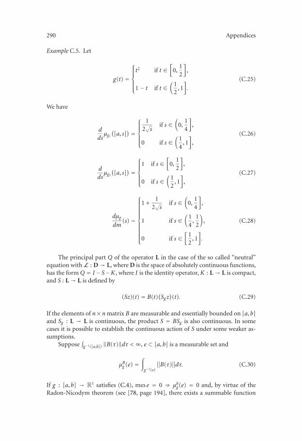
290 Appendices
Example C.5. Let
g(t) =
⎧⎪⎪⎪⎨
⎪⎪⎪⎩
t2 if t ∈[
0,12
],
1− t if t ∈(
12
, 1].
(C.25)
We have
d
dsμg1
([a, s]
) =
⎧⎪⎪⎪⎨
⎪⎪⎪⎩
12√s
if s ∈(
0,14
],
0 if s ∈(
14
, 1]
,
(C.26)
d
dsμg2
([a, s]
) =
⎧⎪⎪⎪⎨
⎪⎪⎪⎩
1 if s ∈[
0,12
],
0 if s ∈(
12
, 1]
,
(C.27)
dμgdm
(s) =
⎧⎪⎪⎪⎪⎪⎪⎪⎪⎪⎨
⎪⎪⎪⎪⎪⎪⎪⎪⎪⎩
1 +1
2√s
if s ∈(
0,14
],
1 if s ∈(
14
,12
),
0 if s ∈[
12
, 1].
(C.28)
The principal part Q of the operator L in the case of the so called “neutral”equation with L : D → L, where D is the space of absolutely continuous functions,has the form Q = I−S−K , where I is the identity operator, K : L → L is compact,and S : L → L is defined by
(Sz)(t) = B(t)(Sgz)(t). (C.29)
If the elements of n×n matrix B are measurable and essentially bounded on [a, b]and Sg : L → L is continuous, the product S = BSg is also continuous. In somecases it is possible to establish the continuous action of S under some weaker as-sumptions.
Suppose∫g−1([a,b]) ‖B(τ)‖dτ <∞, e ⊂ [a, b] is a measurable set and
μBg (e) =∫
g−1(e)
∥∥B(τ)
∥∥dτ. (C.30)
If g : [a, b] → R1 satisfies (C.4), mes e = 0 ⇒ μbg(e) = 0 and, by virtue of theRadon-Nicodym theorem (see [78, page 194], there exists a summable function
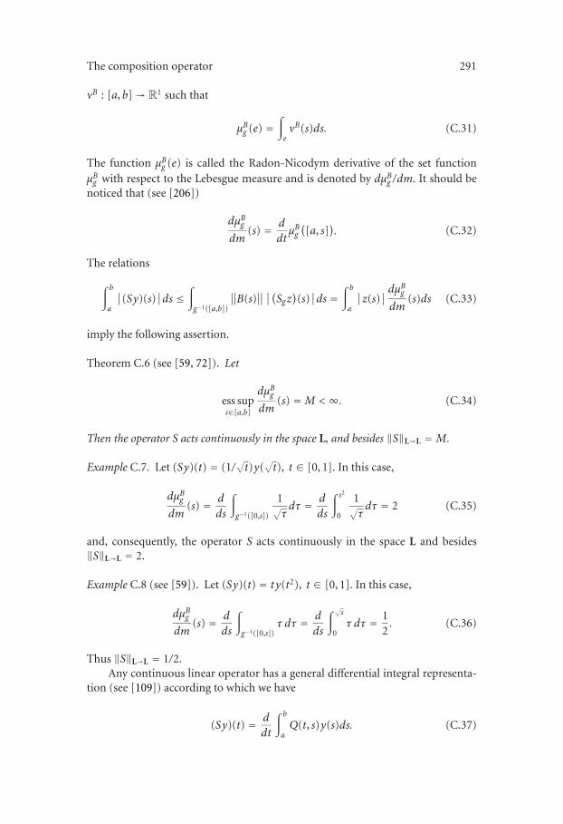
The composition operator 291
νB : [a, b] → R1 such that
μBg (e) =∫
eνB(s)ds. (C.31)
The function μBg (e) is called the Radon-Nicodym derivative of the set functionμBg with respect to the Lebesgue measure and is denoted by dμBg /dm. It should benoticed that (see [206])
dμBgdm
(s) = d
dtμBg([a, s]
). (C.32)
The relations
∫ b
a
∣∣(Sy)(s)∣∣ds ≤
∫
g−1([a,b])
∥∥B(s)∥∥∣∣(Sgz
)(s)∣∣ds =
∫ b
a
∣∣z(s)∣∣dμBgdm
(s)ds (C.33)
imply the following assertion.
Theorem C.6 (see [59, 72]). Let
ess sups∈[a,b]
dμBgdm
(s) =M <∞. (C.34)
Then the operator S acts continuously in the space L, and besides ‖S‖L→L =M.
Example C.7. Let (Sy)(t) = (1/√t)y(
√t), t ∈ [0, 1]. In this case,
dμBgdm
(s) = d
ds
∫
g−1([0,s])
1√τdτ = d
ds
∫ s2
0
1√τdτ = 2 (C.35)
and, consequently, the operator S acts continuously in the space L and besides‖S‖L→L = 2.
Example C.8 (see [59]). Let (Sy)(t) = ty(t2), t ∈ [0, 1]. In this case,
dμBgdm
(s) = d
ds
∫
g−1([0,s])τ dτ = d
ds
∫ √s
0τ dτ = 1
2. (C.36)
Thus ‖S‖L→L = 1/2.Any continuous linear operator has a general differential integral representa-
tion (see [109]) according to which we have
(Sy)(t) = d
dt
∫ b
aQ(t, s)y(s)ds. (C.37)
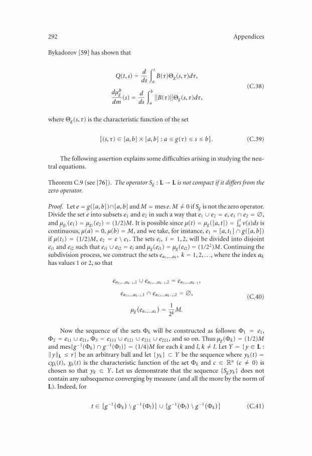
292 Appendices
Bykadorov [59] has shown that
Q(t, s) = d
ds
∫ t
aB(τ)Θg(s, τ)dτ,
dμBgdm
(s) = d
ds
∫ b
a
∥∥B(τ)
∥∥Θg(s, τ)dτ,
(C.38)
where Θg(s, τ) is the characteristic function of the set
{(s, τ) ∈ [a, b]× [a, b] : a ≤ g(τ) ≤ s ≤ b
}. (C.39)
The following assertion explains some difficulties arising in studying the neu-tral equations.
Theorem C.9 (see [76]). The operator Sg : L → L is not compact if it differs from thezero operator.
Proof. Let e = g([a, b])∩[a, b] andM = mes e.M �= 0 if Sg is not the zero operator.Divide the set e into subsets e1 and e2 in such a way that e1 ∪ e2 = e, e1 ∩ e2 = ∅,and μg1 (e1) = μg2 (e2) = (1/2)M. It is possible since μ(t) = μg([a, t]) = ∫ ta ν(s)ds iscontinuous, μ(a) = 0, μ(b) = M, and we take, for instance, e1 = [a, t1]∩ g([a, b])if μ(t1) = (1/2)M, e2 = e \ e1. The sets ei, i = 1, 2, will be divided into disjointei1 and ei2 such that ei1 ∪ ei2 = ei and μg(ei1) = μg(ei2) = (1/22)M. Continuing thesubdivision process, we construct the sets eα1,...,αk , k = 1, 2, . . ., where the index αkhas values 1 or 2, so that
eα1,...,αk−1,1 ∪ eα1,...,αk−1,2 = eα1,...,αk−1 ,
eα1,...,αk−1,1 ∩ eα1,...,αk−1,2 = ∅,
μg(eα1,...,αk
) = 12kM.
(C.40)
Now the sequence of the sets Φk will be constructed as follows: Φ1 = e1,Φ2 = e11 ∪ e21, Φ3 = e111 ∪ e121 ∪ e211 ∪ e221, and so on. Thus μg(Φk) = (1/2)Mand mes{g−1(Φk) ∩ g−1(Φl)} = (1/4)M for each k and l, k �= l. Let Y = {y ∈ L :‖y‖L ≤ r} be an arbitrary ball and let {yk} ⊂ Y be the sequence where yk(t) =cχk(t), χk(t) is the characteristic function of the set Φk and c ∈ Rn (c �= 0) ischosen so that yk ∈ Y . Let us demonstrate that the sequence {Sg yk} does notcontain any subsequence converging by measure (and all the more by the norm ofL). Indeed, for
t ∈ {g−1(Φk) \ g−1(Φl
)}∪ {g−1(Φl) \ g−1(Φk
)}(C.41)
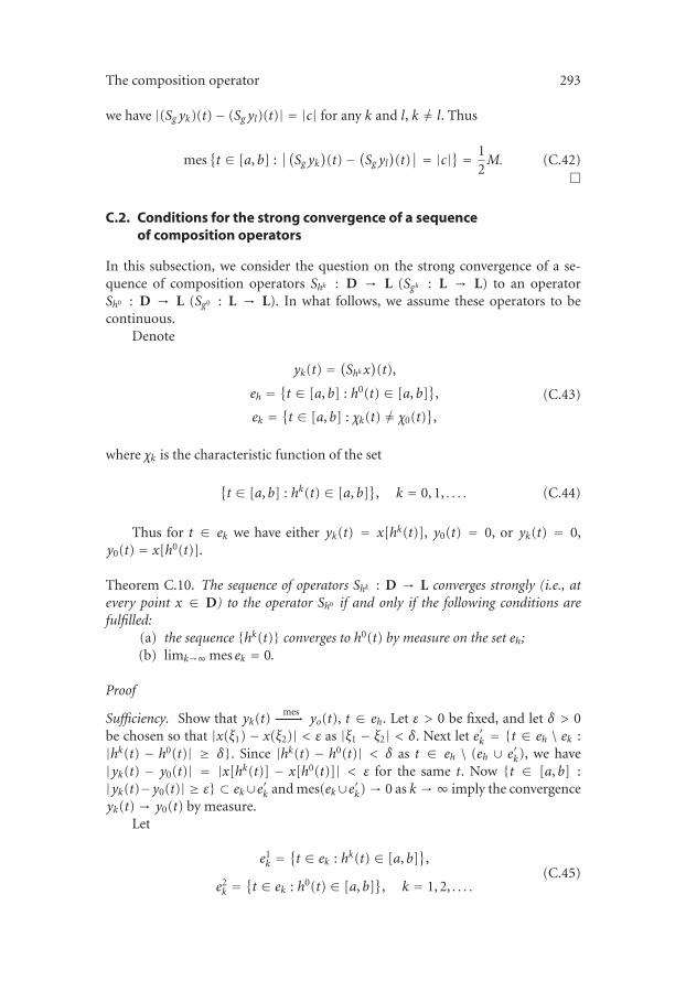
The composition operator 293
we have |(Sg yk)(t)− (Sg yl)(t)| = |c| for any k and l, k �= l. Thus
mes{t ∈ [a, b] :
∣∣(Sg yk)(t)− (Sg yl
)(t)∣∣ = |c|} = 1
2M. (C.42)
�
C.2. Conditions for the strong convergence of a sequenceof composition operators
In this subsection, we consider the question on the strong convergence of a se-quence of composition operators Shk : D → L (Sgk : L → L) to an operatorSh0 : D → L (Sg0 : L → L). In what follows, we assume these operators to becontinuous.
Denote
yk(t) = (Shkx)(t),
eh ={t ∈ [a, b] : h0(t) ∈ [a, b]
},
ek ={t ∈ [a, b] : χk(t) �= χ0(t)
},
(C.43)
where χk is the characteristic function of the set
{t ∈ [a, b] : hk(t) ∈ [a, b]
}, k = 0, 1, . . . . (C.44)
Thus for t ∈ ek we have either yk(t) = x[hk(t)], y0(t) = 0, or yk(t) = 0,y0(t) = x[h0(t)].
Theorem C.10. The sequence of operators Shk : D → L converges strongly (i.e., atevery point x ∈ D) to the operator Sh0 if and only if the following conditions arefulfilled:
(a) the sequence {hk(t)} converges to h0(t) by measure on the set eh;(b) limk→∞ mes ek = 0.
Proof
Sufficiency. Show that yk(t)mes������������������������������������������������������������������������������→ yo(t), t ∈ eh. Let ε > 0 be fixed, and let δ > 0
be chosen so that |x(ξ1) − x(ξ2)| < ε as |ξ1 − ξ2| < δ. Next let e′k = {t ∈ eh \ ek :|hk(t) − h0(t)| ≥ δ}. Since |hk(t) − h0(t)| < δ as t ∈ eh \ (eh ∪ e′k), we have|yk(t) − y0(t)| = |x[hk(t)] − x[h0(t)]| < ε for the same t. Now {t ∈ [a, b] :|yk(t)−y0(t)| ≥ ε} ⊂ ek∪e′k and mes(ek∪e′k) → 0 as k →∞ imply the convergenceyk(t) → y0(t) by measure.
Let
e1k =
{t ∈ ek : hk(t) ∈ [a, b]
},
e2k =
{t ∈ ek : h0(t) ∈ [a, b]
}, k = 1, 2, . . . .
(C.45)
294 Appendices
Then,
∥∥yk − y0
∥∥
L =∫
eh\ek
∣∣yk(s)− y0(s)
∣∣ds +
∫
e1k
∣∣yk(s)
∣∣ds +
∫
e2k
∣∣y0(s)
∣∣ds. (C.46)
The first of the integrals tends to zero as k → ∞ by virtue of the Lebesguetheorem, the second as well as the third tends to zero, being estimated by the valuemaxt∈[a,b] |x(t)|mes ek.
Necessity. By setting x(t) = col{t, 0, . . . , 0}, we obtain
∣∣y1
k(t)− y10(t)
∣∣ =
⎧⎪⎪⎪⎪⎪⎪⎨
⎪⎪⎪⎪⎪⎪⎩
∣∣hk(t)− h0(t)
∣∣ if t ∈ eh \ ek,
∣∣hk(t)∣∣ if t ∈ e1
k ,
∣∣h0(t)
∣∣ if t ∈ e2
k.
(C.47)
Therefore, hk(t)mes���������������������������������������������������������������������������������������������������������→ h0(t) on eh and mes ek → 0. �
Consider now the sequence of operators Tk : D → L defined by
(Tkx
)(t) = Pk(t)
(Shkx
)(t) (C.48)
measurable on [a, b] elements of n× n matrices Pk.
Theorem C.11. Let the following conditions be fulfilled:(a) ‖Pk(t)− P0(t)‖ → 0 by measure on eh as k →∞;(b) there exists a summable function ρ : [a, b] → R1 such that
∥∥Pk(t)
∥∥ ≤ ρ(t), t ∈ [a, b], k = 0, 1, . . . ; (C.49)
(c) hk(t) → h0(t) by measure on eh as k →∞;(d) limk→∞ mes ek = 0.
Then limk→∞ ‖Tkx − T0x‖L = 0 for any x ∈ D.
Proof. The following inequality is valid:
∥∥Tkx − T0x
∥∥
L ≤∫ b
a
∥∥Pk(s)− P0(s)
∥∥∣∣yk(s)
∣∣ds
+∫ b
a
∥∥P0(s)
∥∥∣∣yk(s)− y0(s)
∣∣ds = Ik1 + Ik2 .
(C.50)
The composition operator 295
Consider each of the integrals individually:
Ik1 =∫
eh\ek
∥∥Pk(s)− P0(s)∥∥ · ∣∣yk(s)
∣∣ds +∫
e1k
∥∥Pk(s)− P0(s)∥∥∣∣yk(s)
∣∣ds
+∫
ek2
∥∥Pk(s)− P0(s)
∥∥∣∣y0(s)
∣∣ds.
(C.51)
The first term in the right-hand side of the latter equality tends to zero as k → ∞by virtue of the Lebesgue theorem. The second and the third are estimated by
2 maxt∈[a,b]
∣∣x(t)
∣∣∫
ekρ(s)ds. (C.52)
In the same way with the equality
Ik2=∫
eh\ek
∥∥P0(s)
∥∥∣∣yk(s)−y0(s)
∣∣ds +
∫
e1k
∥∥P0(s)
∥∥∣∣yk(s)
∣∣ds +
∫
e2k
∥∥P0(s)
∥∥∣∣y0(s)
∣∣ds,
(C.53)
one can establish that limk→∞ Ik2 = 0. �
Remark C.12. The conditions (c) and (d) of Theorem C.11 can be replaced by theweaker ones:
(c′) hk(t) → h0(t) by measure on {t ∈ eh : ‖P0(t)‖ �= 0};(d′) limk→∞ mes{t ∈ eh : ‖P0(t)‖ �= 0} = 0.Conditions for the strong convergence of a sequence {Sgk}, Sgk : L → L, have
been established by M. E. Drakhlin and T. K. Plyshevskaya. Here we formulate thecorresponding results without proof. Denote
Eg ={t ∈ [a, b] : g0(t) ∈ [a, b]
},
Ek ={t ∈ [a, b] : χk(t) �= χ0(t)
},
(C.54)
where χk is the characteristic function of the set
{t ∈ [a, b] : gk(t) ∈ [a, b]
}, k = 0, 1, . . . . (C.55)
Theorem C.13 (see [76]). The sequence of operators Sgk : L → L converges to Sg0 ateach point of the space L if and only if the following conditions are fulfilled:
(a) gk(t) → g0(t) by measure on Eg ;(b) limk→∞ mes Ek = 0;(c) the norms of the operators Sgk , k = 1, 2, . . . , are uniformly bounded.
Remark C.14. In [77], it is shown that the strong convergence of the operatorsSgk : L → L to Sg0 : L → L is equivalent to the weak convergence of these operatorsto Sg0 : L → L.
296 Appendices
Consider now the sequence of operators Sk : L → L defined by
(Sk y
)(t) = Bk(t)
(Sgk y
)(t), (C.56)
where the elements of n × n matrices Bk are measurable and essentially boundedon [a, b]. It is not difficult to show that the sequence {Sk} converges to S0 at everypoint y ∈ L under the following conditions: limk→∞ ‖Sgk y − Sg0 y‖L = 0 for everyy ∈ L; ‖Bk(t) − B0(t)‖ → 0 by measure on Eg as k → ∞ with the addition thatthere exists an essentially bounded function ρ : [a, b] → R1 such that ‖Bk(t)‖ ≤ρ(t), t ∈ [a, b], for all k.
The following theorem gives a more subtle test for the strong convergence of{Sk}.
Denote
μBk
gk (e) =∫
(gk)−1(e)
∥∥Bk(s)∥∥ds, (C.57)
where νk(s) = (dμBk
gk /dm)(s) is the Radon-Nicodym derivative of function μBk
gk withrespect to the Lebesgue measure (see [78]).
Theorem C.15 (see [73]). Let the following conditions be fulfilled:(a) ‖Bk(t)− B0(t)‖ → 0 by measure on Eg as k →∞;(b) supk ess sups∈[a,b] νk(s) <∞;(c) gk(t) → g0(t) by measure on {t ∈ Eg : ‖B0(t)‖ �= 0};(d) limk→∞ mes{t ∈ Ek : ‖B0(t)‖ �= 0} = 0.
Then limk→∞ ‖Sk y − S0y‖L = 0 for any y ∈ L.
D. Vallee-Poussin-like theorem
An exclusive place in the theory of differential equation
(Lx)(t)def= x(t) + q(t)x(t) + p(t)x(t) = 0 (D.1)
is occupied by the interval [a, b] on which any nontrivial solution has at mostone zero. Such an interval is called the nonoscillation interval (of the solutions ofLx = 0).
From the Sturm theorem on separation of zeros of solutions to Lx = 0, itfollows that [a, b] is the nonoscillation interval if and only if there exists a positivesolution of Lx = 0 on [a, b].
Vallee-Poussin criterion [69]. An interval [a, b] is the nonoscillation interval forLx = 0 if and only if there exists a function v : [a, b] → R1 with absolutely continu-ous derivative v such that
v(t) ≥ 0, (Lv)(t) ≤ 0 for t ∈ [a, b], v(a) + v(b)−∫ b
a(Lv)(s)ds > 0.
(D.2)
Vallee-Poussin-like theorem 297
A proper choice of the comparison function v permits getting on the baseof the Vallee-Poussin criterion the estimates of the length of the nonoscillationinterval. It should be noted that the Vallee-Poussin criterion was known before thementioned estimates.
The interest to the nonoscillation interval may be explained by a link betweenthe existence of a positive solution and many actual problems. Such a link is estab-lished by the next theorem.
Theorem D.1. The following assertions are equivalent.(a) [a, b] is the nonoscillation interval.(b) There exists a v : [a, b] → R1 with absolutely continuous derivative v such
that
v(t) ≥ 0, (Lv)(t) ≤ 0, t ∈ [a, b], v(a) + v(b)−∫ b
a(Lv)(s)ds > 0.
(D.3)
(c) The Cauchy function C(t, s) of the equation Lx = f is strictly positive inthe triangle a ≤ s < t ≤ b.
(d) The two-point boundary value problem
Lx = f , x(a) = 0, x(b) = 0 (D.4)
is uniquely solvable for each summable f , and the Green function of thisproblem is strictly negative in the square (a, b)× (a, b).
It should be noticed that due to well-known results of Jacobi, the listof the equivalent assertions of Theorem D.1 may be added by the followingassertion.
(e) There exists a unique function v : [a, b] → R1 with absolutely continuousderivative v on which the functional
∫ b
aexp
∫ s
aq(τ)dτ
[x2(s)− p(s)x2(s)
]ds (D.5)
with the conditions x(a) = 0, x(b) = 0 reaches its minimum.
The equivalence of (a) and (c) had been established by Wilkins [223].The equivalence of (a) and (d) had been established by Pack [168].It is natural to name Theorem D.1 after Vallee-Poussin. A wide series of in-
vestigations by various authors has been devoted to the extension of this theoremupon equations of higher order and delay differential equations. Below we offera general assertion on the base of which it is possible to prove some variants ofVallee-Poussin-like theorems for a wide class of functional differential equations.
Let B be a Banach space of measurable z : [a, b] → Rn, let C be a Banachspace of continuous x : [a, b] → Rn, let D be a Banach space of x : [a, b] → Rn
298 Appendices
isomorphic to the direct product B × Rn, and, besides, let the elements of D becontinuous on [a, b].
Consider the boundary value problem
Lx = f , lx = α (D.6)
under the following assumptions.The linear L : D → B is bounded and Noether with ind L = n. The com-
ponents l1, . . . , ln of the vector functional l = [l1, . . . , ln] are linear bounded func-tionals on the space D. If there are functionals among li such that lix = x(νi),νi ∈ [a, b], the set of all such points νi is denoted by {ν}; otherwise the symbol {ν}indicates the empty set.
Further we assume that the decomposition L = L0−T holds, where T : C →B is bounded and isotonic (antitonic) and the linear L0 : D → B possesses thefollowing properties.
(1) The boundary value problem
L0x = f , lx = α (D.7)
has a unique solution x ∈ D for each { f ,α} ∈ B × Rn and besides theGreen operator W of this problem is isotonic (antitonic).
(2) There exists ψ ∈ B such that ψ(t) ≥ 0 (ψ(t) ≤ 0) a.e. on [a, b] and(Wψ)(t) > 0 for t ∈ [a, b] \ {ν}.
(3) There exists a positive solution u0 (u0(t) > 0 for t ∈ [a, b] \ {ν}) of thehomogeneous equation L0x = 0.
As for these properties, it should be noticed that in some cases the properties(1) and (3) are equivalent. For instance, in the case of the problem
x(t) + p(t)x(t) = f (t), x(a) = α1, x(b) = α2, (D.8)
such equivalence follows from Theorem D.1. In the general case, such a connectionmay be absent as it is demonstrated by the example of the problem
x(t) + x(t) = f (t), x(b − a
2
)= α1, x
(b− a
2
)= α2 (D.9)
if π < b − a < 2π. Indeed, the solution u(t) = c1 cos t + c2 sin t is not positive on[a, b] if b − a > π. But the Green operator is isotonic because the Green functionW(t, s) is defined by
W(t, s) =
⎧⎪⎪⎪⎪⎪⎪⎪⎨
⎪⎪⎪⎪⎪⎪⎪⎩
sin(t − s) ifb− a
2≤ s ≤ t ≤ b,
− sin(t − s) if a ≤ t < s ≤ b − a2
,
0 at the other points of the square [a, b]× [a, b].
(D.10)
Vallee-Poussin-like theorem 299
The condition (2) is fulfilled, for instance, if the Green operator W is actingfrom the space Wn of (n − 1) times differentiable functions with absolutely con-tinuous derivative of the order n− 1 into the space L of summable functions. TheGreen operator W : L → Wn is integral (Section 2.3):
(W f )(t) =∫ b
aW(t, s) f (s)ds. (D.11)
As ψ we may take any ψ ∈ L such that ψ(t) > 0 (ψ(t) < 0) a.e. on [a, b]. Indeed,for such ψ the equality (Wψ)(τ) = 0 is possible only for τ ∈ {ν}.
It is relevant to note that condition (2) is fulfilled for not all the integral Greenoperators: if W : L → D, D = {x ∈ Wn : x(ξ) = 0, ξ ∈ [a, b]}, the equality(W f )(ξ) = 0 holds for any f ∈ L.
Denote A =WT . The problem (D.6) is equivalent to the equation
x = Ax + y, (D.12)
where y is the solution of the model problem L0x = f , lx = α. The equation maybe considered in the space C since the values of A on continuous functions belongto D. Denote by ρ(A) the spectral radius of A : C → C.
Theorem D.2. The following assertions are equivalent.(a) There exists v ∈ D such that
v(t) > 0, r(t)def= (Wϕ)(t) + g(t) > 0, t ∈ [a, b] \ {ν}, (D.13)
where ϕ = Lv, g is the solution of the semihomogeneous problem
L0x = 0, lx = lv. (D.14)
(b) ρ(A) < 1.(c) The problem (D.6) has a unique solution x ∈ D for each { f ,α} ∈ B×Rn
and, besides, the Green operator G of this problem is isotonic (antitonic).(d) The homogeneous equation Lx = 0 has a positive solution u (u(t) > 0 for
t ∈ [a, b] \ {ν}) such that lu = lu0.
Proof. Let (a) hold. The function v as a solution of Lx = ϕ satisfies (D.12) for y =Wϕ+g = r. Therefore, v−Av = r. If {ν} is empty, the implication (a)⇒(b) followsfrom Lemma A.1, if {ν} is not empty, the implication follows from Theorem A.3.
Since ρ(A) < 1, the implication (b)⇒(c) follows from the fact that the solutionx of (D.12) exists and may be presented in the form
x = y + Ay + A2y + · · · . (D.15)
Hence
G = (I + A + A2 + · · · )W. (D.16)
300 Appendices
To prove the implication (c)⇒(a) let us use ψ ∈ B such that ψ(t) ≥ 0 (ψ(t) ≤0), (Wψ)(t) > 0 for t ∈ [a, b] \ {ν}. Since G is isotonic (antitonic), the functionv = Gψ does not take negative values. Therefore, v(t) = (Av)(t) + (Wψ)(t) > 0and r(t) = (Wψ)(t) > 0, t ∈ [a, b] \ {ν}.
The implication (b)⇒(d) follows from the fact that the estimate ρ(A) < 1guarantees the unique solvability of the problem (D.6) and the representation inthe form
u = u0 + Au0 + A2u0 + · · · (D.17)
of the solution u to the semihomogeneous problem Lx = 0, lx = lu0. Therefore,u(t) ≥ u0(t), t ∈ [a, b].
Taking v = u, we get the implication (d)⇒(a). �
Remark D.3. If W and G are integral operators, the list of the equivalent asser-tions of Theorem C.10 may be added by the one on the fact that G(t, s) ≥W(t, s)(G(t, s) ≤W(t, s)), where W(t, s) and G(t, s) are the kernels of the integral opera-tors.
Remark D.4. In the case of the second-order differential equation the assertion (d)on the existence of a positive solution is equivalent to the assertion of nonoscilla-tion.
Remark D.5. The proof of the equivalence of the assertions (a), (b), and (c) doesnot use the property (3).
Turning back to the equation
(Lx)(t)def= x(t) + q(t)x(t) + p(t)x(t) = f (t), (D.18)
we will prove Theorem D.1 assuming the coefficients q and p to be summable.
Proof of Theorem D.1. First consider an auxiliary lemma using the specific charac-ter of ordinary differential equations.
Lemma D.6. The following assertions are equivalent.(a) [a, b] is the nonoscillation interval for Lx = 0.(b) The Cauchy function C(t, s) of the equation Lx = f is strictly positive in
the triangle a ≤ s < t ≤ b.(c) The two-point boundary value problem
Lx = f , x(a) = x(b) = 0 (D.19)
is uniquely solvable and the Green function G(t, s) of the problem is strictlynegative in the square (a, b)× (a, b).
Vallee-Poussin-like theorem 301
Proof.
C(t, s) = 1W(s)
∣∣∣∣∣∣
u1(s) u2(s)
u1(t) u2(t)
∣∣∣∣∣∣
, a ≤ s ≤ t ≤ b, (D.20)
where u1, u2 constitute the fundamental system for Lx = 0, W is the Wron-skian of the system. From this representation of C(t, s), it is clear that the sectionCs(t) = C(t, s) for each fixed s ∈ [a, b) is a solution of Lx = 0 on [s, b]. Now(a)⇒(b) follows from the conditions Cs(s) = 0, (d/ds)Cs(s) = 1 which guaranteeCs(t) > 0 on (s, b]. The implication (b)⇒(a) follows from Sturm’s theorem on theseparation of zeros and the inequality Ca(t) > 0, t ∈ (a, b].
Theorem 2.4 yields the following properties of Green function G(t, s). Foreach fixed s ∈ (a, b) the section gs(t) = G(t, s) of the Green function is continuouson [a, b], on each interval [a, s) or (s, b] the section gs satisfies the homogeneousequation Lx = 0 and the boundary conditions gs(a) = gs(b) = 0. Besides,
gs(s + 0)− gs(s− 0) = 1. (D.21)
Let (a) be fulfilled, let s ∈ (a, b) be fixed, let vs be the solution of the problem
Lx = 0, x(s) = 0, x(s) = 1, (D.22)
and let us be the solution of the two-point problem
Lx = 0, x(a) = 0, x(b) = vs(b). (D.23)
The latter problem is uniquely solvable since vs(t) > 0. The section gs may berepresented as
gs(t) = χ[s,b](t)vs(t)− us(t), (D.24)
where χ[s,b] is the characteristic function of the interval [s, b]. The section gs haszeros only at the points a and b by virtue of the nonoscillation. Thus gs(t) < 0,t ∈ (a, b), whence (c) follows.
Let (c) be fulfilled. The solution y of the problem
Lx = 0, x(a) = 0, x(a) = 1 (D.25)
is proportional to the function gs on the interval [a, s]. The assumption that y(b) =0 leads to contradiction: under such an assumption y is a nontrivial solution of the
302 Appendices
homogeneous problem
Lx = 0, x(a) = x(b) = 0. (D.26)
Thus y(t) < 0 on (a, b]. Hence (a) follows by Sturm’s theorem. Thus Lemma D.6is proved. �
Next let us show that the conditions of Theorem D.2 are fulfilled for the equa-tion Lx = f .
Let p = p+ − p−, p+(t), p−(t) ≥ 0, L0x = x + qx − p−x. Then
Lx = L0x + p+x. (D.27)
The equation Mxdef= x + qx = 0 has the solution x(t) ≡ 1. Therefore, by the
Sturm theorem, [a, b] is an nonoscillation interval for the equation. By LemmaD.6, the Cauchy function CM(t, s) for the equationMx = f is positive. The Cauchyproblem
L0xdef= x + qx − p−x = 0, x(a) = 1, x(a) = 0 (D.28)
is equivalent to the equation x = Kx + 1 with isotonic Volterra operator
(Kx)(t) =∫ t
aCM(t, s)p−(s)x(s)ds. (D.29)
Thus the solution u0 of the latter equation is positive:
u0(t) = 1 +(K[1]
)(t) +
(K2[1]
)(t) + · · · ≥ 1, (D.30)
and so [a, b] is the nonoscillation interval for the model equation L0x = 0. Itfollows, by Lemma D.6, that the model problem
L0x = f , x(a) = x(b) = 0 (D.31)
is uniquely solvable and the Green function W(t, s) of the problem is strictly neg-ative in the square (a, b) × (a, b). Besides there exists a solution of the equationL0x = 0 such that u0(t) > 0 for t ∈ (a, b), u0(a) + u0(b) > 0. �
Bibliography
[1] R. R. Akhmerov, M. I. Kamenskiı, A. S. Potapov, A. E. Rodkina, and B. N. Sadovskiı, Measures ofNoncompactness and Condensing Operators, Operator Theory: Advances and Applications, vol.55, Birkhuser, Basel, 1992.
[2] G. Alefeld and J. Herzberger, Introduction to Interval Computations, Computer Science and Ap-plied Mathematics, Academic Press, New York, 1983.
[3] V. M. Alekseev, E. M. Galeev, and V. M. Tikhomirov, Collection of problems on optimization,Theory. Examples. Problems, Nauka, Moscow, 1984.
[4] V. M. Alekseev, V. M. Tikhomirov, and S. V. Fomin, Optimal Control, Nauka, Moscow, 1979.
[5] M. J. Alves, Singular functional differential equation of the second order: Diss. kand. phys.-matem.nauk, Perm. University, Perm, 1999. 114 p. (Russian).
[6] T. Ando, Positive linear operators in semi-ordered linear spaces, Journal of the Faculty of Science,Hokkaido University Series I 13 (1957), 214–228.
[7] E. A. Andreeva, V. B. Kolmanovskiı, and L. E. Shaıkhet, Control of Systems with Aftereffect, Nauka,Moscow, 1992, English translation in Translations of Mathematical Monographs, vol. 157, AMS,1996.
[8] A. V. Anokhin, On linear impulse system for functional differential equations, Doklady AkademiiNauk USSR 286 (1986), no. 5, 1037–1040 (Russian).
[9] , On the continuous dependence of the solution of an abstract functional-differential equa-tion on the parameters, Functional-Differential Equations, Perm. Politekh. Inst., Perm, 1990, pp.142–145.
[10] , Linear functional differential equations with impulsive effects: Diss. kand. phys.-matem.nauk, Perm. Politekh. Inst., Perm, 1984. 137 p. (Russian).
[11] A. V. Anokhin and L. F. Rakhmatullina, Continuous dependence of the solution of a linear bound-ary value problem on the parameters, Izvestiya Vysshikh Uchebnykh Zavedeniı. Matematika(1996), no. 11, 29–38 (Russian).
[12] A. B. Antonevich and Yu. A. Bykadorov, On operators of the form (Sy)(t) = a(t)y(α(t)) associatedwith functional differential equations, (Russian) Minsk, 1985. 54 p. Dep. in VINITI 21.03.85, No.2043-85.
[13] M. Ashordia, On the stability of solutions of the multipoint boundary value problem for the systemof generalized ordinary differential equations, Memoirs on Differential Equations and Mathemat-ical Physics 6 (1995), 1–57, 134.
[14] , On the correctness of nonlinear boundary value problems for systems of generalized ordi-nary differential equations, Georgian Mathematical Journal 3 (1996), no. 6, 501–524.
[15] , Conditions of existence and uniqueness of solutions of the multipoint boundary value prob-lem for a system of generalized ordinary differential equations, Georgian Mathematical Journal 5(1998), no. 1, 1–24.
[16] N. V. Azbelev, Linear boundary value problems for functional-differential equations, Differ-entsial’nye Uravneniya 10 (1974), no. 4, 579–584, 763 (Russian).
[17] , The Perm seminar and the development of the theory of functional-differential equations,Functional-Differential Equations (Russian), Perm. Politekh. Inst., Perm, 1985, pp. 3–12.
[18] , Two hypotheses in the theory of functional differential equations, Uspehi Matematich-eskih Nauk 41 (1986), no. 4, 210–211 (Russian).
[19] , The problems and prospects of the Perm seminar on the theory of functional differentialequations, I, Functional-Differential Equations, Perm Politekh. Inst., SPF “Prognoz”, Perm, 1992,pp. 3–14.
304 Bibliography
[20] , Recent state and trends of developing of the theory of functional differential equations,Izvestiya Vysshikh Uchebnykh Zavedeniı. Matematika (1994), no. 6, 8–19 (Russian).
[21] , The ideas and methods of the Perm seminar on boundary value problems, Boundary ValueProblems for Functional-Differential Equations (J. Henderson, ed.), World Scientific, New Jer-sey, 1995, pp. 13–22.
[22] N. V. Azbelev, M. Zh. Alvesh, and E. I. Bravyı, On singular boundary value problems for a second-order linear functional-differential equation, Izvestiya Vysshikh Uchebnykh Zavedeniı. Matem-atika (1999), no. 2, 3–11 (Russian).
[23] N. V. Azbelev, M. P. Berdnikova, and L. F. Rakhmatullina, Integral equations with deviating ar-gument, Doklady Akademii Nauk SSSR 192 (1970), no. 3, 479–482 (Russian).
[24] N. V. Azbelev, L. M. Berezanskiı, and L. F. Rakhmatullina, A linear functional-differential equa-tion of evolution type, Differentsial’nye Uravneniya 13 (1977), no. 11, 1915–1925, 2106 (Rus-sian).
[25] N. V. Azbelev, L. M. Berezanskiı, P. M. Simonov, and A. V. Chistyakov, The stability of linearsystems with aftereffect. I, Differentsial’nye Uravneniya 23 (1987), no. 5, 745–754, 914 (Russian).
[26] , The stability of linear systems with aftereffect. IV, Differentsial’nye Uravneniya 29 (1993),no. 2, 196–204, 364 (Russian).
[27] N. V. Azbelev, E. I. Bravyı, and S. A. Gusarenko, On effective sufficient conditions for the solvabilityof variational problems, Doklady Akademii Nauk 381 (2001), no. 2, 151–154 (Russian).
[28] , On effective sufficient conditions for solvability of variational problems, Functional Dif-ferential Equations 9 (2002), no. 1-2, 57–70.
[29] N. V. Azbelev and A. I. Domoshnitskiı, On de la Vallee Poussin’s differential inequality, Differ-entsial’nye Uravneniya 22 (1986), no. 12, 2041–2045, 2203 (Russian).
[30] N. V. Azbelev and G. G. Islamov, To the theory of abstract linear equation, Functional-DifferentialEquations, Perm. Politekh. Inst., Perm, 1989, pp. 3–16.
[31] N. V. Azbelev and V. P. Maksimov, Equations with retarded argument, Differentsial’nye Urav-neniya 18 (1982), no. 12, 2027–2050, 2206 (Russian).
[32] N. V. Azbelev, V. P. Maksimov, and L. F. Rakhmatullina, Introduction to the Theory of Functional-Differential Equations, Nauka, Moscow, 1991.
[33] , Introduction to the Theory of Linear Functional-Differential Equations, Advanced Seriesin Mathematical Science and Engineering, vol. 3, World Federation, Georgia, 1995.
[34] N. V. Azbelev and L. F. Rakhmatullina, Linear equations with deviating argument, Differ-entsial’nye Uravneniya 6 (1970), no. 4, 616–628 (Russian).
[35] , Functional-differential equations, Differentsial’nye Uravneniya 14 (1978), no. 5, 771–797, 955 (Russian).
[36] , To the question on functional differential inequalities and monotone operators,Functional-Differential Equations, Perm. Politekh. Inst., Perm, 1986, pp. 3–9.
[37] , An abstract functional-differential equation, Functional-Differential Equations (Rus-sian), Perm. Politekh. Inst., Perm, 1987, pp. 3–11.
[38] , On extension of the Vallee-Poussin theorem to equations with aftereffect, Boundary ValueProblems for Functional-Differential Equations (J. Henderson, ed.), World Scientific, New Jer-sey, 1995, pp. 23–36.
[39] , Theory of linear abstract functional-differential equations and applications, Memoirs onDifferential Equations and Mathematical Physics 8 (1996), 1–102.
[40] N. V. Azbelev, L. F. Rakhmatullina, and A. G. Terentiev, W-method in studying of differen-tial equations with deviated argument, Trudy Tambovskogo Instituta Khimicheskogo Mashinos-troeniya, Tambov (1970b), 60–63 (Russian).
[41] N. V. Azbelev and P. M. Simonov, Stability of Differential Equations with Aftereffect, Stability andControl: Theory, Methods and Applications, vol. 20, Taylor & Francis, London, 2003.
[42] N. V. Azbelev and T. S. Sulavko, On the question of the stability of the solutions of differentialequations with retarded argument, Differentsial’nye Uravneniya 10 (1974), no. 12, 2091–2100,2307 (Russian).
Bibliography 305
[43] N. V. Azbelev and Z. B. Tsalyuk, On integral inequalities, Matematicheskii Sbornik 59 (1962),no. 3, 325–341 (Russian).
[44] , Integral and differential inequalities, Proceedings of the Fourth All-Union MathematicalCongress, Vol. 2, Nauka, Moscow, 1965.
[45] N. S. Bakhvalov, Numerical Methods (Analysis, Algebra, Ordinary Differential Equations), Izdat.Nauka, Moscow, 1973.
[46] E. A. Barbashin, Introduction to the Stability Theory, Nauka, Moscow, 1967.
[47] M. Barszch and A. W. Olbrot, Stability criterion for a linear differential-difference system, IEEETransactions on Automatic Control 24 (1979), no. 2, 368–369.
[48] A. I. Bashkirov, Stability of solutions of periodic systems with aftereffect: Diss. kand. phys.-matem.nauk, Perm, 1986, 102 p. (Russian).
[49] P. R. Beesack, On the Green’s function of an N-point boundary value problem, Pacific Journal ofMathematics 12 (1962), no. 3, 801–812.
[50] G. S. Bondareva, Multipoint problem for a generalized Poisson equation, Izvestiya InstitutaMatematiki i Informatiki. Izdatel’stvo Udmurtskogo Universiteta (1994), no. 2, 25–33 (Russian).
[51] , Multipoint problem for the Poisson equation, Izvestiya Instituta Matematiki i Infor-matiki. Izdatel’stvo Udmurtskogo Universiteta (1998), no. 4, 81–104 (Russian).
[52] , Multipoint problem for the Poisson equation: Diss. kand. phys.-matem. nauk, Udmurt.Univ., Izhevsk, 1999. (Russian).
[53] E. I. Bravyı, Solvability of a boundary value problem for a nonlinear singular functional-differentialequation, Izvestiya Vysshikh Uchebnykh Zavedeniı. Matematika (1993), no. 5, 17–23.
[54] , On the regularization of singular functional-differential equations, Differentsial’nyeUravneniya 30 (1994), no. 1, 26–34, 180 (Russian).
[55] , Linear functional differential equations with inner singularities: Diss. kand. phys.-matem.nauk, Perm. Gos. Tekh. Univ., Perm, 1996. 107 p. (Russian).
[56] S. A. Brykalov, A priori estimates and the solvability of problems with nonlinear functional bound-ary conditions, Differentsial’nye Uravneniya 35 (1999), no. 7, 874–881, 1005 (Russian).
[57] A. L. Bukhgeım, Volterra Equations and Inverse Problems, “Nauka” Sibirsk. Otdel., Novosibirsk,1983.
[58] A. I. Bulgakov and L. N. Lyapin, On the connectedness of the solutions set of the inclusion with theVolterra operator, Boundary Value Problems, Perm. Politekh. Inst., Perm, 1980, pp. 146–149.
[59] Yu. A. Bykadorov, On the boundedness of the composition operator, Boundary Value Problems,Perm. Politekh. Inst., Perm, 1980, pp. 177–179.
[60] H. Cartan, Calcul Differentiel. Formes Differentielles, Hermann, Paris, 1967.[61] E. S. Chichkin, A theorem on a differential inequality for multi-point boundary-value problems,
Izvestiya Vysshikh Uchebnykh Zavedeniı. Matematika 1962 (1962), no. 2 (27), 170–179 (Rus-sian).
[62] A. V. Chistyakov, Properties of a class of noncompact operators, Functional-Differential Equations(Russian), Perm. Politekh. Inst., Perm, 1988, pp. 21–29.
[63] , Spectral properties of operators of inner superposition that are generated by stochasticsystems, Functional-Differential Equations (Russian), Perm. Politekh. Inst., Perm, 1991, pp. 101–112.
[64] , A pathological counterexample to the non-Fredholmness conjecture in algebras of weightedshift operators, Izvestiya Vysshikh Uchebnykh Zavedeniı. Matematika (1995), no. 10, 76–86 (Rus-sian).
[65] S. Cinquini, Sulle eqationi funzionali del typo di Volterra, Rendiconti della Reale Academia deiLincei 17 (1933), 616–621.
[66] L. Collatz, Functional Analysis and Computational Mathematics, Mir, Moscow, 1969.[67] C. Corduneanu, Integral Equations and Applications, Cambridge University Press, Cambridge,
1991.[68] G. F. Corliss, Where is validated ODE solving going?, Proceedings of the IMACS-GAMM Inter-
national Symposium on Numerical Methods and Error Bounds (G. Alefeld and J. Herzberger,eds.), Mathematical Research, vol. 89, Akademie, Berlin, 1996, pp. 48–57.
306 Bibliography
[69] Ch. I. de La Vallee-Poussin, Sur l’equation differentielle lineare du second ordre, Journal deMathematiques Pures et Appliquees 8 (1929), no. 9, 125–144.
[70] V. Ya. Derr, The sign of the Green function of a generalized de la Vallee-Poussin problem,Functional-Differential Equations (Russian), Perm. Politekh. Inst., Perm, 1986, pp. 35–41.
[71] A. I. Domoshnitskiı, A version of N. V. Azbelev’s W-method and the monotonicity of the Greenoperator for boundary value problems with distributed functionals in the boundary conditions,Functional-Differential Equations (Russian), Perm. Politekh. Inst., Perm, 1990, pp. 161–168.
[72] M. E. Drakhlin, The composition operator in the space of summable functions, Izvestiya VysshikhUchebnykh Zavedeniı. Matematika (1986), no. 5, 18–23 (Russian).
[73] , Convergence of a sequence of inner superposition operators, Boundary Value Problems(Russian), Perm. Politekh. Inst., Perm, 1989, pp. 179–184.
[74] M. E. Drakhlin and L. M. Kultysheva, On composition operator in the spaces of Orlicz, BoundaryValue Problems (Russian), Perm. Politekh. Inst., Perm, 1977, pp. 126–130.
[75] M. E. Drakhlin and M. A. Makagonova, Euler functional-differential equations, Functional-Differential Equations (Russian), Perm. Politekh. Inst., Perm, 1987, pp. 12–18.
[76] M. E. Drakhlin and T. K. Plysevskaja, On the theory of functional-differential equations, Differ-entsial’nye Uravneniya 14 (1978), no. 8, 1347–1361, 1529 (Russian).
[77] M. E. Drakhlin and E. Stepanov, Weak convergence of inner superposition operators, Proceedingsof the American Mathematical Society 126 (1998), no. 1, 173–179.
[78] N. Dunford and J. T. Schwartz, Part I: General Theory, John Wiley & Sons, New York, 1958.[79] R. J. Elliott, Stochastic Calculus and Applications, Applications of Mathematics (New York), vol.
18, Springer, New York, 1982.[80] M. Emery, Une topologie sur l’espace des semimartingales, Seminaire de Probabilites, XIII (Univ.
Strasbourg, Strasbourg, 1977/1978), Lecture Notes in Math., vol. 721, Springer, Berlin, 1979, pp.260–280.
[81] N. P. Erugin, et al., Main directions of the development of the ordinary differential equation theory,History of the Native Mathematics, vol. 4, book 1, Naukova Dumka, Kiev, 1970, pp. 453–478,Scientific groups and centers.
[82] A. Feintuch and R. Saeks, System Theory. A Hilbert Space Approach, Pure and Applied Mathe-matics, vol. 102, Academic Press, New York, 1982.
[83] E. M. Galeev and V. M. Tikhomirov, A Short Course on the Theory of Extremal Problems, Izda-tel’stvo Moskovskogo Universiteta, Moscow, 1989.
[84] P. Gambosh, Statistical Theory of the Atom and Its Applications, Izdatel’stvo Inostrannoi Liter-atury, Moscow, 1951.
[85] S. K. Godunov, Ordinary Differential Equations with Constant Coefficient, Translations of Math-ematical Monographs, vol. 169, American Mathematical Society, Rhode Island, 1997.
[86] I. C. Gokhberg and M. G. Kreın, Theory of Volterra Operators in Hilbert Space and Its Applica-tions, Izdat. Nauka, Moscow, 1967.
[87] D. Graffi, Sorpa una equazioine funczionale e la sua applicazione a un problema di fisica ereditaria,Annali di Matematica Pura ed Applicata 9 (1931), 143–179.
[88] A. A. Gruzdev, Reduction of extremal problems to linear equations in a Hilbert space, IzvestiyaVysshikh Uchebnykh Zavedeniı. Matematika (1993), no. 5, 36–42 (Russian).
[89] , Boundary value problems for functional differential equations in the study of variationalproblems for square functionals: Diss. kand. phys.-matem. nauk, Perm. Gos. Tekh. Univ., 1997.78 p. (Russian).
[90] A. A. Gruzdev and S. A. Gusarenko, On the reduction of variational problems to extremal problemswithout constraints, Izvestiya Vysshikh Uchebnykh Zavedeniı. Matematika (1994), no. 6, 39–49(Russian).
[91] S. A. Gusarenko, A generalization of the concept of a Volterra operator, Doklady Akademii NaukSSSR 295 (1987), no. 5, 1046–1049.
[92] , Conditions for the solvability of problems on the accumulation of perturbations forfunctional-differential equations, Functional-Differential Equations (Russian), Perm. Politekh.Inst., Perm, 1987, pp. 30–40.
Bibliography 307
[93] , The generalized Volterra property and its applications to a linear functional-partial differ-ential equation, Functional-Differential Equations (Russian), Perm. Politekh. Inst., Perm, 1989,pp. 53–57.
[94] , On variational problems with linear constraints, Izvestiya Vysshikh Uchebnykh Zave-deniı. Matematika (1998), no. 1, 1–15 (Russian).
[95] S. A. Gusarenko, E. S. Zhukovskiı, and V. P. Maksimov, On the theory of functional-differentialequations with locally Volterra operators, Soviet Mathematics. Doklady 33 (1986), no. 2, 368–371.
[96] A. Halanay, Differential Equations: Stability, Oscillations, Time Lags, Academic Press, New York,1966.
[97] A. Halanay and D. Wexler, Qualitative Theory of Impulse Systems, Mir, Moscow, 1971.
[98] J. Hale, Theory of Functional Differential Equations, Springer, New York, 1977.
[99] P. Halmos, Measure Theory, Izdatel’stvo Inostrannoi Literatury, Moscow, 1953.
[100] V. Hutson and J. S. Pym, Applications of Functional Analysis and Operator Theory, Mathematicsin Science and Engineering, vol. 146, Academic Press, New York, 1980.
[101] G. G. Islamov, On an estimate of the spectral radius of the linear positive compact operator,Functional-Differential Equations and Boundary Value Problems in Mathematical Physics,Perm. Politekh. Inst., Perm, 1978, pp. 119–122.
[102] , Some applications of the theory of an abstract functional-differential equation. I, Differ-entsial’nye Uravneniya 25 (1989), no. 11, 1872–1881, 2019 (Russian).
[103] , Some applications of the theory of an abstract functional-differential equation. II, Differ-entsial’nye Uravneniya 26 (1990), no. 2, 224–232, 364 (Russian).
[104] , On an upper bound for the spectral radius, Doklady Akademii Nauk USSR 322 (1992),no. 5, 836–838 (Russian).
[105] J. Jacod, Calcul stochastique et problemes de martingales, Lecture Notes in Mathematics, vol. 714,Springer, Berlin, 1979.
[106] , Weak and strong solutions of stochastic differential equations, Stochastics 3 (1980), no. 3,171–191.
[107] J. Jacod and J. Memin, Existence of weak solutions for stochastic differential equations with drivingsemimartingales, Stochastics 4 (1981), no. 4, 317–337.
[108] L. V. Kantorovich and G. P. Akilov, Functional Analysis, 3rd ed., Nauka, Moscow, 1984.[109] L. V. Kantorovich, B. Z. Vulikh, and A. G. Pinsker, Functional Analysis in Partially Ordered Spaces,
Gostekhizdat, Moscow, 1950.[110] E. W. Kaucher and W. L. Miranker, Self-Validating Numerics for Function Space Problems, Aca-
demic Press, New York, 1988.[111] A. Ya. Khokhryakov, An information on the Izhevsk seminar, Differentsial’nye Uravneniya 1
(1965), no. 12, 1686–1687 (Russian).[112] I. T. Kiguradze, Some Singular Boundary Value Problems for Ordinary Differential Equations, Iz-
datel’stvo Tbilisskogo Universiteta, Tbilisi, 1975.[113] I. T. Kiguradze and B. L. Shekhter, Singular boundary value problems for second-order ordinary
differential equations, Current Problems in Mathematics. Newest Results, Vol. 30 (Russian), ItogiNauki i Techniki. Ser. Sovremennye Problemy Matematiki: Novye Dostigeniya, Akad. Nauk SSSRVsesoyuz. Inst. Nauchn. i Tekhn. Inform., Moscow, 1987, pp. 105–201, 204.
[114] A. A. Kirillov and A. D. Gvishiani, Theorems and Problems of Functional Analysis, Nauka,Moscow, 1979.
[115] V. B. Kolmanovskiı and V. R. Nosov, Stability of Functional-Differential Equations, Mathematicsin Science and Engineering, vol. 180, Academic Press, London, 1986.
[116] A. N. Kolmogorov and S. V. Fomin, Elements of the Theory of Functions and Functional Analysis,6th ed., Nauka, Moscow, 1989.
[117] M. A. Korytova, On an estimate of the spectral radius for certain linear operators, Functional-Differential Equations, Perm. Politekh. Inst., Perm, 1992, pp. 239–245.
[118] , Some constructive methods in the theory of functional differential equations: Diss. kand.phys.-matem. nauk, Perm. Politekh. Inst., Perm, 1993. 87 p. (Russian).
308 Bibliography
[119] M. A. Krasnosel’skiı and P. P. Zabreıko, Geometric Methods of Nonlinear Analysis, Monographsin Nonlinear Analysis and Applications, Nauka, Moscow, 1975.
[120] M. A. Krasnosel’skiı, P. P. Zabreıko, E. I. Pustyl’nik, and P. E. Sobolevskiı, Integral Operators inSpaces of Summable Functions, Nauka, Moscow, 1966.
[121] N. N. Krasovskiı, Certain Problems in the Theory of Stability of Motion, Gosudarstv. Izdat. Fiz.-Mat. Lit., Moscow, 1959.
[122] S. G. Krein, Linear Equations in Banach Space, Nauka, Moscow, 1971.[123] L. D. Kudryavtsev, The variational method of searching for generalized solutions of differential
equations in function spaces with power weight, Differentsial’nye Uravneniya 19 (1983), no. 10,1723–1740 (Russian).
[124] , Existence and uniqueness of solutions of variational problems, Doklady Akademii NaukSSSR 298 (1988), no. 5, 1055–1060 (Russian).
[125] G. P. Kukhta, A remark with respect the conditions L∗ and L∗∗ of N. V. Azbelev, Uchenye ZapiskiKishinevskogo Universiteta (Phys. Math.) 29 (1957), 49–52 (Russian).
[126] S. Yu. Kultyshev, The controllability of linear functional-differential systems, Differentsial’nyeUravneniya 11 (1975), no. 8, 1355–1360, 1529 (Russian).
[127] S. Yu. Kultyshev and E. L. Tonkov, Controllability of a linear nonstationary system, Differ-entsial’nye Uravneniya 11 (1975), no. 7, 1206–1216, 1348 (Russian).
[128] L. M. Kultysheva, On equations with the composition operator: Diss. kand. phys-matem. nauk,Perm. Politekh. Inst., Perm, 1981. (Russian).
[129] V. G. Kurbatov, Linear functional-differential equations of neutral type, and the retarded spectrum,Sibirskiı Matematiceskiı Zurnal 16 (1975), no. 3, 538–550, 644 (Russian).
[130] , Linear Differential-Difference Equations, Voronezhskiı Gosudarstvennyı Universitet,Voronezh, 1990.
[131] , Functional-Differential Operators and Equations, Mathematics and Its Applications, vol.473, Kluwer Academic, Dordrecht, 1999.
[132] N. S. Kurpel’ and B. A. Shuvar, Two-Sided Operator Inequalities and Their Applications, NaukovaDumka, Kiev, 1980.
[133] Ja. Kurzweil, Generalized ordinary differential equations and continuous dependence on a param-eter, Czechoslovak Mathematical Journal 7 (82) (1957), 418–449.
[134] , On continuous dependence on parameter in the theory of ordinary differential equationsand on the generalization of the concept of differential equations, Uspehi Matematicheskih Nauk12 (1957a), no. 5, 257–259 (Russian).
[135] , Generalized ordinary differential equations, Czechoslovak Mathematical Journal 8 (83)(1958), 360–388.
[136] S. M. Labovskiı, Positive solutions of a two-point boundary value problem for a linear singu-lar functional-differential equation, Functional-Differential Equations (Russian), Perm. Politekh.Inst., Perm, 1985, pp. 39–45, iv.
[137] N. N. Likhacheva, On Differential Inequalities for Equations with Deviated Argument, Perm. Po-litehk. Inst., Perm, 1989, 16 p., Dep. in VINITI 04.04.89, N 2467-89.
[138] , The de la Vallee-Poussin theorem for a classs of functional-differential equations, IzvestiyaVysshikh Uchebnykh Zavedeniı. Matematika (1997), no. 5, 30–37.
[139] A. G. Lomtatidze and S. Mukhigulashvili, Some Two-Point Boundary Value Problems for SecondOrder Functional Differential Equation, Folia Facultatis Scientiarium Naturalium UniversitatisMasarykianae Brunensis. Mathematica, vol. 8, Masaryk University, Brno, 2000.
[140] N. N. Luzin, On the method of approximate integration of academician S. A. Chaplygin, UspekhiMatematicheskikh Nauk 6 (1951), no. 6(46), 3–27 (Russian).
[141] V. P. Maksimov, The property of being Noetherian of the general boundary value problem for alinear functional differential equation, Differentsial’nye Uravneniya 10 (1974), no. 12, 2288–2291,2312 (Russian).
[142] , The Cauchy formula for a functional-differential equation, Differentsial’nye Uravneniya13 (1977), no. 4, 601–606, 770–771.
[143] , Some nonlinear boundary value problems, Differentsial’nye Uravneniya 19 (1983), no. 3,396–414 (Russian).
Bibliography 309
[144] , Linear functional differential equation: Diss. kand. phys.-matem. nauk, Tambov Inst.Khim. Mashinostr., Tambov, 1974. (Russian).
[145] , The questions of the general theory of functional differential equations: Diss. doct. phys.-matem. nauk, Perm. Politekh. Inst., Perm, 1984. (Russian).
[146] V. P. Maksimov and J. S. P. Munembe, On the question of enclosing solutions of linear functional-differential systems, Memoirs on Differential Equations and Mathematical Physics 12 (1997),149–156.
[147] V. P. Maksimov and A. N. Rumyantsev, The study of the solvability of boundary value problemsusing the computer systems for analytical calculations, Boundary Value Problems, Perm. Politekh.Inst., Perm, 1986, pp. 3–6.
[148] , Boundary value problems and problems of impulse control in economic dynamics. Con-structive investigation, Izvestiya Vysshikh Uchebnykh Zavedeniı. Matematika 37 (1993), no. 5,48–62.
[149] , The study of the solvability of boundary value problems for functional-differential equa-tions: a constructive approach, Boundary Value Problems for Functional-Differential Equations(J. Henderson, ed.), World Scientific, New Jersey, 1995, pp. 227–237.
[150] , Constructive methods in the theory of functional-differential equations and their computeraided implementation, Functional Differential Equations 4 (1997), no. 1-2, 133–141 (1998).
[151] V. P. Maksimov, A. N. Rumyantsev, and V. A. Shishkin, On constructing solutions of functional-differential systems with a guaranteed precision, Functional Differential Equations 3 (1995), no. 1-2, 135–144.
[152] J. L. Massera and J. J. Schaeffer, Linear Differential Equations and Function Spaces, Pure andApplied Mathematics, vol. 21, Academic Press, New York, 1966.
[153] S. G. Mikhlin, Course of Mathematical Physics, Nauka, Moscow, 1968.
[154] V. D. Mil’man and A. D. Myshkis, On the stability of motion in the presence of impulses, SibirskiıMatematiceskiı Zurnal 1 (1960), no. 2, 233–237 (Russian).
[155] V. J. Mizel and V. Trutzer, Stochastic hereditary equations: existence and asymptotic stability, Jour-nal of Integral Equations 7 (1984), no. 1, 1–72.
[156] S.-E. A. Mohammed, Stochastic Functional Differential Equations, Research Notes in Mathemat-ics, vol. 99, Pitman (Advanced Publishing Program), Massachusetts, 1984.
[157] , Lyapunov exponents and stochastic flows of linear and affine hereditary systems: a survey,Research Report 91-98, Department of Mathematics, Carnegie Mellon University, Pennsylvania,January 1991.
[158] R. E. Moore, A test for existence of solutions to nonlinear systems, SIAM Journal on NumericalAnalysis 14 (1977), no. 4, 611–615.
[159] R. E. Moore and Z. H. Shen, Interval methods for operator equations, Reliability in Computing (R.E. Moore, ed.), Perspect. Comput., vol. 19, Academic Press, Massachusetts, 1988, pp. 379–389.
[160] J. S. P. Munembe, On a stabilization problem for the trajectories of nonlinear functional differentialsystems with periodic parameters, Some Problems in Fundamental and Applied Mathematics,Moscow Phys.-Tekhn. Inst., Moscow, 1998, pp. 106–115.
[161] , On the question of asymptotic behaviour of the solutions to linear functional differentialequations with delay and periodic parameters, Izvestiya Vysshikh Uchebnykh Zavedeniı. Matem-atika (2000), no. 4, 28–35 (Russian).
[162] I. Muntean, The spectrum of the Cesaro operator, Mathematica. Revue d’Analyse Numerique etde Theorie de l’Approximation 22 (1980), no. 1, 97–105.
[163] A. D. Myshkis, Linear Differential Equations with Delay Argument, Gostekhizdat, Moscow, 1951.[164] , Linear Differential Equations with Retarded Argument, 2nd ed., Izdat. “Nauka”, Moscow,
1972.[165] , Some problems in the theory of differential equations with deviating argument, Uspekhi
Matematicheskikh Nauk 32 (1977), no. 2(194), 173–202, 264 (Russian).[166] I. P. Natanson, Theory of Functions of a Real Variable, 3rd ed., Nauka, Moscow, 1974.[167] T. A. Osechkina, Periodic boundary value problem for functional differential equation: Diss. kand.
phys.-matem. nauk, Perm. Politekh. Inst., Perm, 1994. 101 p. (Russian).
310 Bibliography
[168] S. A. Pack, On differential inequality for the Sturm-Liouville problems, Doklady Academii NaukSSSR 148 (1963), no. 6, 1275–1278 (Russian).
[169] S. V. Parter, Solutions of a differential equation arising in chemical reactor processes, SIAM Journalon Applied Mathematics 26 (1974), no. 4, 687–716.
[170] S. V. Parter, M. L. Stein, and P. R. Stein, On the multiplicity of solutions of a differential equationarising in chemical reactor theory, Studies in Applied Mathematics 54 (1975), no. 4, 293–314.
[171] O. Perron, Die Stabilitatsfrage bei Differentialgleichungen, Mathematische Zeitschrift 32 (1930),no. 1, 703–728.
[172] V. P. Plaksina, Some questions in the theory of impulse boundary value problems: Diss. kand. phys.-matem. nauk, Perm. Politekh. Inst. Perm, 1989. 142 p. (Russian).
[173] M. Plum, Computer-assisted existence proofs for two-point boundary value problems, Computing46 (1991), no. 1, 19–34.
[174] , Existence and enclosure results for continua of solutions of parameter-dependent nonlinearboundary value problems, Journal of Computational and Applied Mathematics 60 (1995), no. 1-2, 187–200.
[175] A. V. Ponosov, On the extensions of local-type operators, Boundary Value Problems, Perm. Po-litekh. Inst, Perm, 1987b, pp. 92–96.
[176] , On the Nemytskii conjecture, Soviet Mathematics. Doklady 34 (1987a), no. 1, 231–233.[177] , A fixed-point method in the theory of stochastic differential equations, Soviet Mathemat-
ics. Doklady 37 (1988), no. 2, 426–429.[178] , A theorem of Schauder type for locally defined operators, Functional-Differential Equa-
tions (Russian), Perm. Politekh. Inst., Perm, 1988, pp. 40–49.[179] , Approximation in the class of Volterra operators, Boundary Value Problems (Russian),
Perm. Politekh. Inst., Perm, 1988, pp. 77–82.[180] , Tightness property for operators associated with the Wiener process, Statistical Methods
(1988c), 148–154 (Russian).[181] , On the theory of reducible Ito equations, Differential Equations 25 (1990), no. 2, 1347–
1355 (Russian).[182] , Local operators and stochastic differential equations, Functional Differential Equations 4
(1997), no. 1-2, 173–189 (1998).[183] Ph. Protter, Stochastic differential equations with feedback in the differentials, Seminar on Proba-
bility, XVI, Lecture Notes in Math., vol. 920, Springer, Berlin, 1982, pp. 459–468.[184] , Volterra equations driven by semimartingales, The Annals of Probability 13 (1985), no. 2,
519–530.[185] L. F. Rakhmatullina, The canonical forms of linear functional-differential equations, Differ-
entsial’nye Uravneniya 11 (1975), no. 12, 2143–2153, 2299 (Russian).[186] , The Green operator and the regularization of linear boundary value problems, Differ-
entsial’nye Uravneniya 15 (1979), no. 3, 425–435, 571–572 (Russian).[187] , Definition of the solution of an equation with deviating argument, Functional-
Differential Equations (Russian), Perm. Politekh. Inst., Perm, 1985, pp. 13–19, i.[188] , The regularization of linear boundary value problems, Izvestiya Vysshikh Uchebnykh
Zavedeniı. Matematika (1987), no. 7, 37–43, 83 (Russian).[189] , The generalized Green operator for an overdetermined boundary value problem for a linear
functional-differential equation, Izvestiya Vysshikh Uchebnykh Zavedeniı. Matematika (1993),no. 5, 95–100 (Russian).
[190] F. Riesz and B. Sz-Nagy, Lecons d’analyse fonctionnelle, Akademiai kiado, Budapest, 1972.[191] J. R. Ringrose, Compact linear operators of Volterra type, Proceedings of the Cambridge Philo-
sophical Society 51 (1955), 44–55.[192] A. N. Rumyantsev, Application of systems of analytic calculations for the study of solvability and
construction of an approximate solution of a class of boundary value problems, Boundary valueproblems (Russian), Perm. Politekh. Inst., Perm, 1987, pp. 74–81.
[193] , Constructive study of dynamic models with pulse perturbations, Functional DifferentialEquations 3 (1995), no. 1-2, 215–222.
Bibliography 311
[194] , The study of the solvability of boundary value problems with impulsive perturbationsby the use of vector a priori inequalities, Izvestiya Vysshikh Uchebnykh Zavedeniı. Matematika(1996), no. 6, 75–82 (Russian).
[195] , Constructive investigation of differential equations with arbitrary deviation of the argu-ment, Izvestiya Vysshikh Uchebnykh Zavedeniı. Matematika (1997), no. 6, 25–31 (Russian).
[196] , Reliable Computer Experiment in the Study of Boundary Value Problems, Izdatel’stvoPermskogo universiteta, Perm, 1999.
[197] , Computer experiment in the study of functional differential models: theory and applica-tions: Diss. doc. phys.-matem. nauk, Perm. Univ., Perm, 1999. 295p. (Russian).
[198] , Constructive study of the solvability of boundary value problems for functional differentialequations: Diss. kand. phys.-matem. nauk, Perm. Politekh. Inst., Perm, 1988. 141 p. (Russian).
[199] A. M. Samoilenko and N. A. Perestyuk, Differential Equations with Impulsive Action, Vishchashkola, Kiev, 1987.
[200] G. Sansone, Sopra un’equazione che si presenta nella determinazione delle orbite in un sincrotrone,Rendiconti della Accademia Nazionale delle Scienze Detta Dei XL. Serie V 8 (1957), 99–172.
[201] M. Scheutzow, Qualitative behaviour of stochastic delay equations with a bounded memory,Stochastics 12 (1984), no. 1, 41–80.
[202] S. Schwabik, Generalized Ordinary Differential Equations, Series in Real Analysis, vol. 5, WorldScientific, New Jersey, 1992.
[203] S. Schwabik, M. Tvrdy, and O. Vejvoda, Differential and Integral Equations. Boundary Value Prob-lems and Adjoints, Academia, Prague, 1979.
[204] L. Schwartz, Theorie des distributions. Tome I, vol. 9, Hermann & Cie., Paris, 1950.[205] , Theorie des distributions. Tome II, vol. 10, Hermann & Cie., Paris, 1951.[206] G. E. Shilov and B. L. Gurevich, Integral, Measure and Derivative. General Theory, Nauka,
Moscow, 1967.[207] A. I. Shindyapin, A boundary value problem for a singular equation, Differentsial’nye Uravneniya
20 (1984), no. 3, 450–455 (Russian).[208] , On the question of singular functional differential equations: Diss. kand. phys.-matem.
nauk, Perm. Politekh. Inst., Perm, 1984. (Russian).[209] I. V. Shragin, Abstract Nemyckii operators are locally defined operators, Soviet Mathematics. Dok-
lady 17 (1976), no. 2, 354–357.[210] S. L. Sobolev, Methode nouvelle a resoudre le probleme de Cauchy pour les equation lineares hyper-
bolic normales, Matematicheskii Sbornik 1 (43) (1936), 39–72.[211] V. S. Sologub, The Development of the Theory of Elliptic Equations in the Eighteenth and Nine-
teenth Centuries, Izdat. “Naukova Dumka”, Kiev, 1975.[212] F. W. Stallard, Functions of bounded variation as solutions of differential systems, Proceedings of
the American Mathematical Society 13 (1962), no. 3, 366–373.[213] V. I. Sumin, Functional Volterra Operators in the Theory Optimal Control of Distributed Systems.
Part I. Volterra Equations and Controlled Initial-Boundary Value Problems, Izdatel’stvo Nizhe-gorodskogo Universiteta, Nizhnii Novgorod, 1992.
[214] A. L. Teptin, Theorems on difference inequalities for n-point difference boundary problems, Matem-aticheskii Sbornik 62 (104) (1963), no. 3, 345–370 (Russian).
[215] A. N. Tikhonov, On functional Volterra type equations and their applications to problems of math-ematical physics, Bulleten’ Moskovsk. Universiteta, Section A 1 (1938), no. 8, 1–25 (Russian).
[216] L. Tonelli, Sulle equazioni funzionali di Volterra, Bulletin of the Calcutta Mathematical Society20 (1929), 31–48.
[217] Ya. Z. Tsypkin, Theory of Impulsive Systems, Phizmatgiz, Moscow, 1958.[218] V. A. Tyshkevich, Some Questions of the Stability Theory of Functional Differential Equations,
Naukova Dumka, Kiev, 1981.[219] M. M. Vaınberg and V. A. Trenogin, Bifurcation Theory of Nonlinear Equations, Nauka, Moscow,
1969.[220] G. M. Vaınikko, Regular convergence of operators and the approximate solution of equations, Math-
ematical Analysis, Vol. 16 (Russian), Itogi nauki i techniki. Ser. matematicheskii analiz, VINITI,Moscow, 1979, pp. 5–53, 151.
312 Bibliography
[221] M. Vath, Abstract Volterra equations of the second kind, Journal of Integral Equations and Appli-cations 10 (1998), no. 3, 319–362.
[222] L. W. Weis, Decompositions of positive operators and some of their applications, Functional Anal-ysis: Surveys and Recent Results, III (Paderborn, 1983), North-Holland Math. Stud., vol. 90,North-Holland, Amsterdam, 1984, pp. 95–115.
[223] J. E. Wilkins Jr., The converse of a theorem of Tchaplygin on differential inequalities, Bulletin ofthe American Mathematical Society 53 (1947), no. 4, 126–129.
[224] L. R. Williams and R. W. Leggett, Multiple fixed point theorems for problems in chemical reactortheory, Journal of Mathematical Analysis and Applications 69 (1979), no. 1, 180–193.
[225] R. Q. Wu and X. Mao, Existence and uniqueness of the solutions of stochastic differential equations,Stochastics (1984), no. 12, 41–80.
[226] D. C. Youla, L. J. Castriota, and H. L. Carlin, Bounded real scattering matrices and the foundationsof linear passive network theory, IRE Transactions on Circuit Theory 6 (1959), no. 1, 102–124.
[227] P. P. Zabreıko, The spectral radius of Volterra integral operators, Litovskii Matematicheskii Sbornik7 (1967), no. 2, 281–287 (Russian).
[228] , Volterra integral operators, Uspekhi Matematicheskikh Nauk 22 (1967), no. 1 (133),167–168 (Russian).
[229] P. P. Zabreıko, A. I. Koshelev, M. A. Krasnosel’skij, S. G. Mikhlin, L. S. Rakovshchik, and V. Ya.Stet’senko, Integral Equations, Noordhoff, Leyden, 1975.
[230] S. T. Zavalishchin and A. N. Sesekin, Impulse Processes: Models and Applications, Nauka, Moscow,1991.
[231] V. Zeidan and P. L. Zezza, Coupled points in the calculus of variations and applications to periodicproblems, Transactions of the American Mathematical Society 315 (1989), no. 1, 323–335.
[232] E. S. Zhukovskiı, On the theory of Volterra equations, Differentsial’nye Uravneniya 25 (1989),no. 9, 1599–1605, 1654 (Russian).
[233] , The Volterra property and spectral properties of an inner superposition operator, Differ-entsial’nye Uravneniya 30 (1994), no. 2, 250–255, 364 (Russian).
[234] , Operator inequalities and functional differential equations: Diss. kand. phys.-matem.nauk, Perm. Politekh. Inst., Perm, 1981. (Russian).
[235] E. S. Zhukovskiı and A. I. Shindyapin, On the problem of the investigation of the solvability ofboundary value problems by the method of a priori inequalities, Boundary Value Problems (Rus-sian), Perm. Politekh. Inst., Perm, 1983, pp. 24–28, 192.
Index
BBoundary value problem, 8
correctly solvable, 226extended, 25linear, 8majorant Cauchy, 244, 246principal, 11
CCanonical a priori inequality, 238
stochastic functional differentialequation, 272
Condition H , 245Connecting system, 30
DDeterminant of the problem, 9
EEquation, 1
B-Volterra-reducible, 236Fredholm, 1linear abstract functional differential, 6majorant, 240, 244model, 16, 92Noether, 1reducible, 214stochastic functional differential, 266Volterra-reducible, 229, 268Volterra-reducible stochastic, 268with aftereffect, 49
FFinite-dimensional part, 7Function, 61
Cauchy, 64computable, 177Green, 61
Fundamental system, 8Fundamental vector, 8
IIndex of the operator, 1
LL1, L2–quasilinearization, 143Local solution, 90Locality, 264
MMatrix, 50
Cauchy, 50Green, 46
OOperator, 1
canonical Fredholm, 8Cauchy, 50, 64composition, 41computable, 178Fredholm, 1generalized Green, 23Green, 13, 61local, 267Nemytskii, 6Noether, 1normal solvable, 1strongly betting, 91tight, 267, 302Volterra, 50Volterra (in the generalized sense), 90
PP -compact, 31P -convergent, 31PQ-convergent, 31Principal part, 7Property, 71
A, 147C, 177, 178Δq , 178Λ, 239P, 71Π, 269
Qq-bettering, 91

314 Index
SSpace, 3
Dπ , 122C, 67D2
p, 167D, 3D(t1, . . . , tn), 117Dr
2, 57DS(m) = DS[a, t1, . . . , tm, b], 100DSn(m), 177L, 3Ln, 177Lr2, 55Lp , 143W2
p , 143Wn, 4, 59WnS(m), 108
TTight, 266Tightness, 264, 266
WW-method, 16, 84W-substitution, 76Weak solutions, 268
![An Introduction to Density Functional Theory · PDF fileAn Introduction to Density Functional Theory N. M. Harrison ... HF [N] N det f f f ... dr = N then E[r t]](https://img.pdfslide.net/doc/110x75/5a9312f47f8b9ad96f8b8f2a/an-introduction-to-density-functional-theory-introduction-to-density-functional.jpg)