Embed Size (px)
Citation preview
Introduction to Theoretical Ecology
Week 1 (Sept. 28, 2021)
Basic introduction to R
1
What is R?
• A programming language and free software that is compatible with different operational systems
• Contains functions for classical and modern statistical data analysis and modeling, as well as graphical functions for data visualization
• Many built-in packages and extensible libraries, also a large user base with extensive help facilities
2
Outline
1. R and R-studio installation
2. Basic computation and data format
3. Data input and processing
4. Data visualization and plotting
5. Create your own function
3
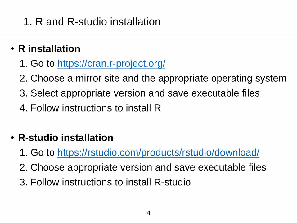
1. R and R-studio installation
• R installation
1. Go to https://cran.r-project.org/
2. Choose a mirror site and the appropriate operating system
3. Select appropriate version and save executable files
4. Follow instructions to install R
• R-studio installation
1. Go to https://rstudio.com/products/rstudio/download/
2. Choose appropriate version and save executable files
3. Follow instructions to install R-studio
4
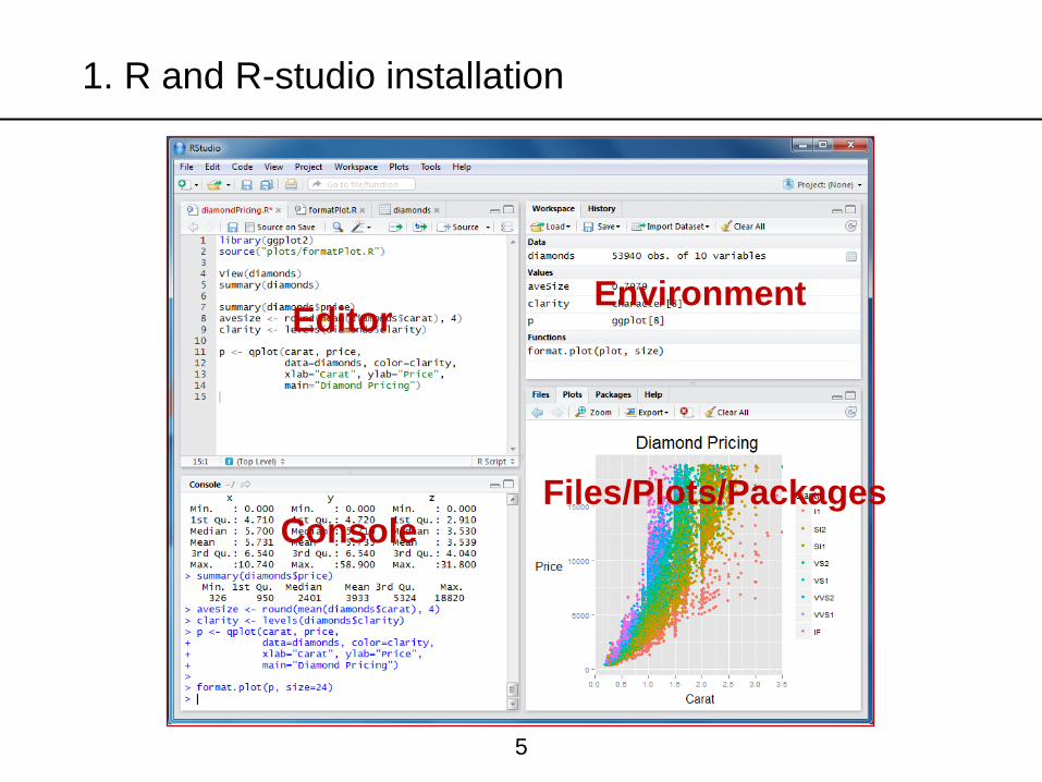
1. R and R-studio installation
Editor
Console
Environment
Files/Plots/Packages
5
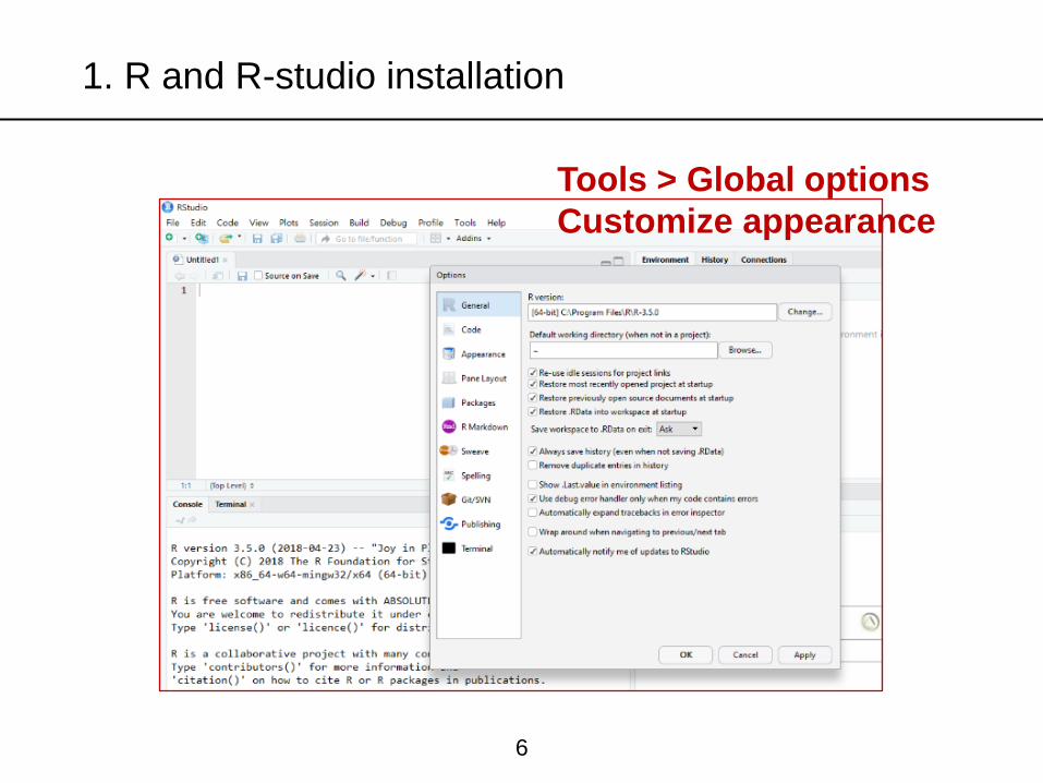
1. R and R-studio installation
Tools > Global options
Customize appearance
6
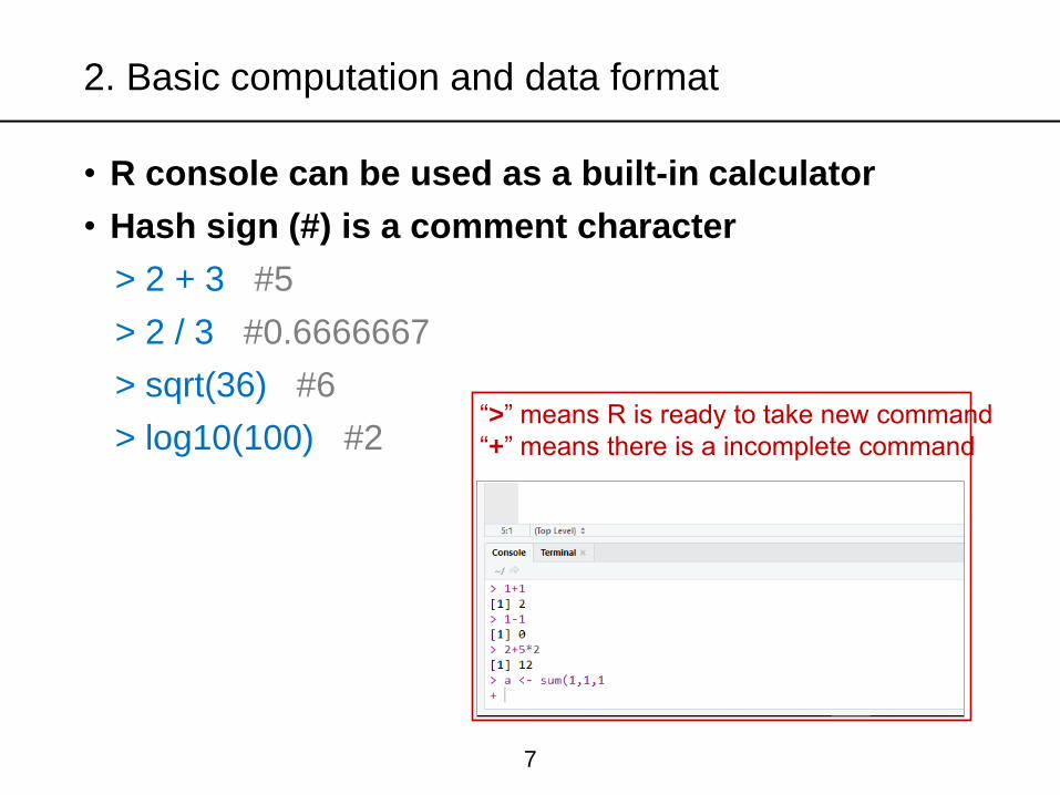
2. Basic computation and data format
• R console can be used as a built-in calculator
• Hash sign (#) is a comment character
> 2 + 3 #5
> 2 / 3 #0.6666667
> sqrt(36) #6
> log10(100) #2
“>” means R is ready to take new command
“+” means there is a incomplete command
7
2. Basic computation and data format
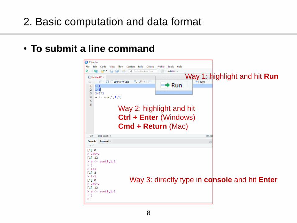
• To submit a line command
8
Way 3: directly type in console and hit Enter
Way 2: highlight and hit
Ctrl + Enter (Windows)
Cmd + Return (Mac)
Way 1: highlight and hit Run
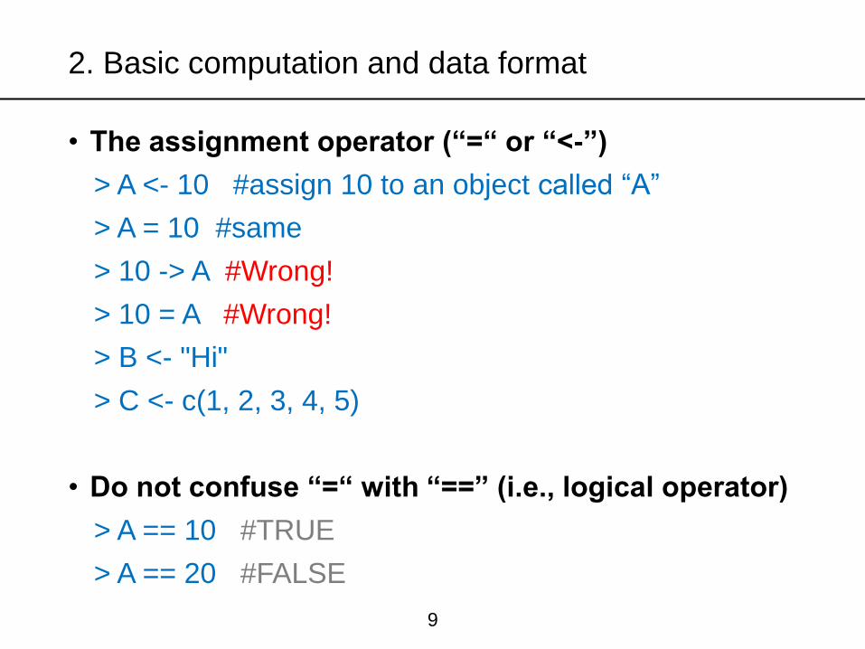
• The assignment operator (“=“ or “<-”)
> A <- 10 #assign 10 to an object called “A”
> A = 10 #same
> 10 -> A #Wrong!
> 10 = A #Wrong!
> B <- "Hi"
> C <- c(1, 2, 3, 4, 5)
• Do not confuse “=“ with “==” (i.e., logical operator)
> A == 10 #TRUE
> A == 20 #FALSE
2. Basic computation and data format
9
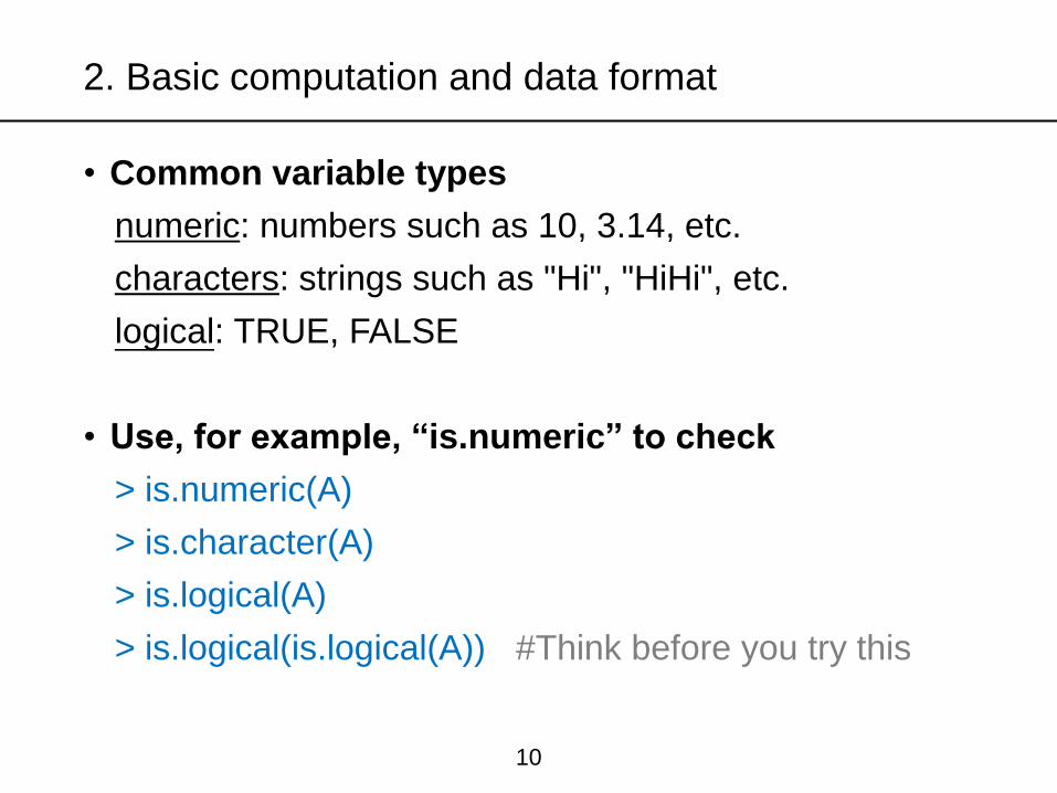
• Common variable types
numeric: numbers such as 10, 3.14, etc.
characters: strings such as "Hi", "HiHi", etc.
logical: TRUE, FALSE
• Use, for example, “is.numeric” to check
> is.numeric(A)
> is.character(A)
> is.logical(A)
> is.logical(is.logical(A)) #Think before you try this
2. Basic computation and data format
10
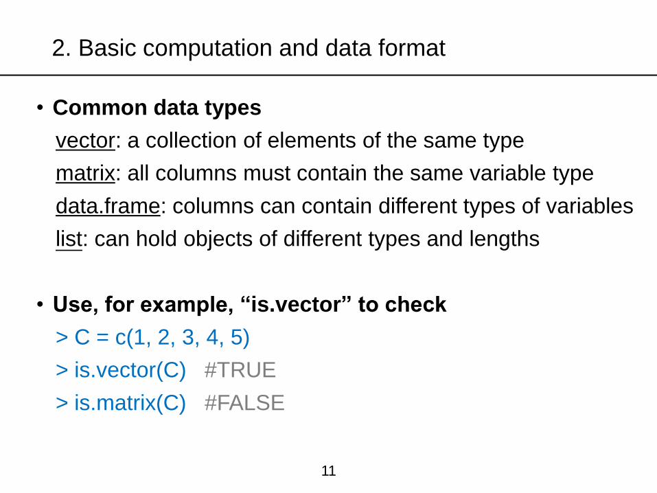
• Common data types
vector: a collection of elements of the same type
matrix: all columns must contain the same variable type
data.frame: columns can contain different types of variables
list: can hold objects of different types and lengths
• Use, for example, “is.vector” to check
> C = c(1, 2, 3, 4, 5)
> is.vector(C) #TRUE
> is.matrix(C) #FALSE
2. Basic computation and data format
11
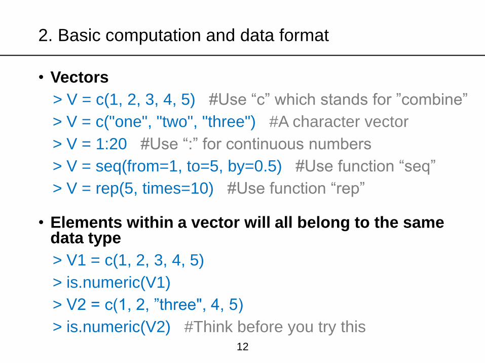
• Vectors
> V = c(1, 2, 3, 4, 5) #Use “c” which stands for ”combine”
> V = c("one", "two", "three") #A character vector
> V = 1:20 #Use “:” for continuous numbers
> V = seq(from=1, to=5, by=0.5) #Use function “seq”
> V = rep(5, times=10) #Use function “rep”
• Elements within a vector will all belong to the same data type
> V1 = c(1, 2, 3, 4, 5)
> is.numeric(V1)
> V2 = c(1, 2, ”three", 4, 5)
> is.numeric(V2) #Think before you try this
2. Basic computation and data format
12
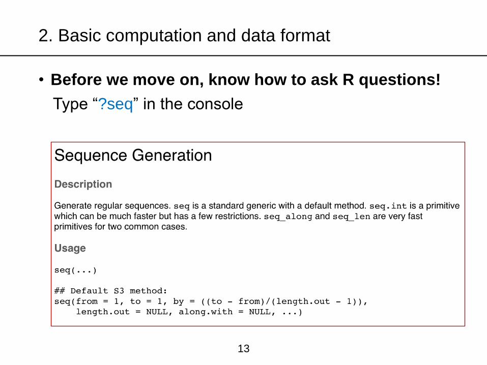
• Before we move on, know how to ask R questions!
Type “?seq” in the console
2. Basic computation and data format
13
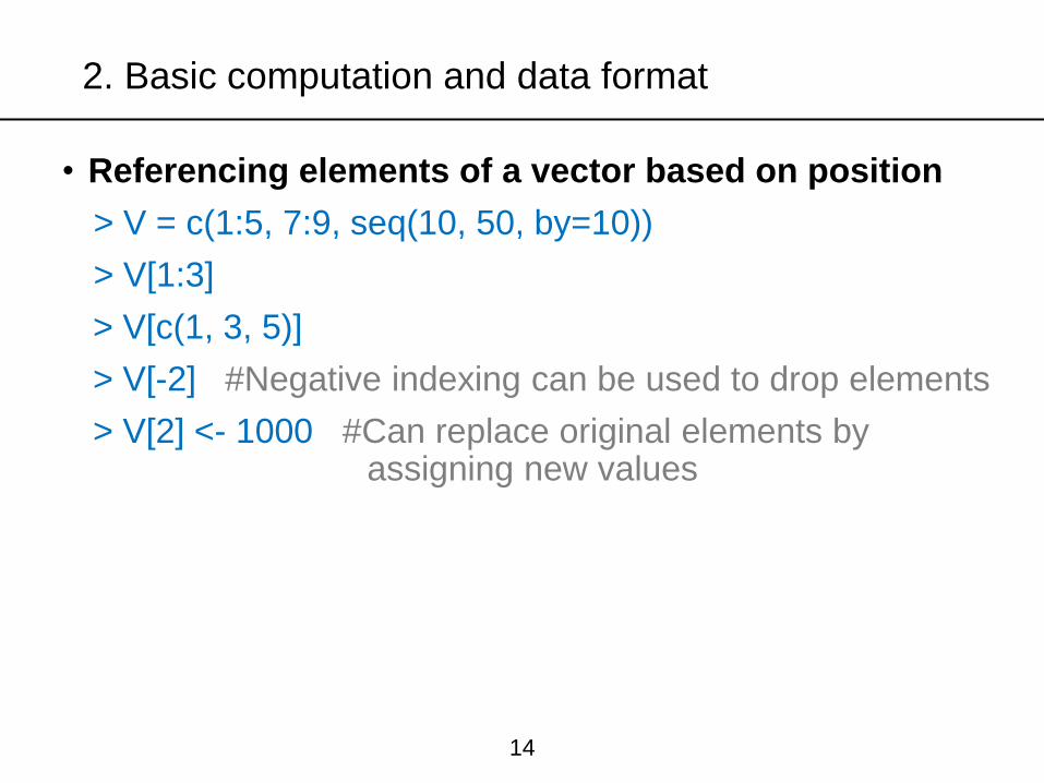
• Referencing elements of a vector based on position
> V = c(1:5, 7:9, seq(10, 50, by=10))
> V[1:3]
> V[c(1, 3, 5)]
> V[-2] #Negative indexing can be used to drop elements
> V[2] <- 1000 #Can replace original elements by assigning new values
2. Basic computation and data format
14
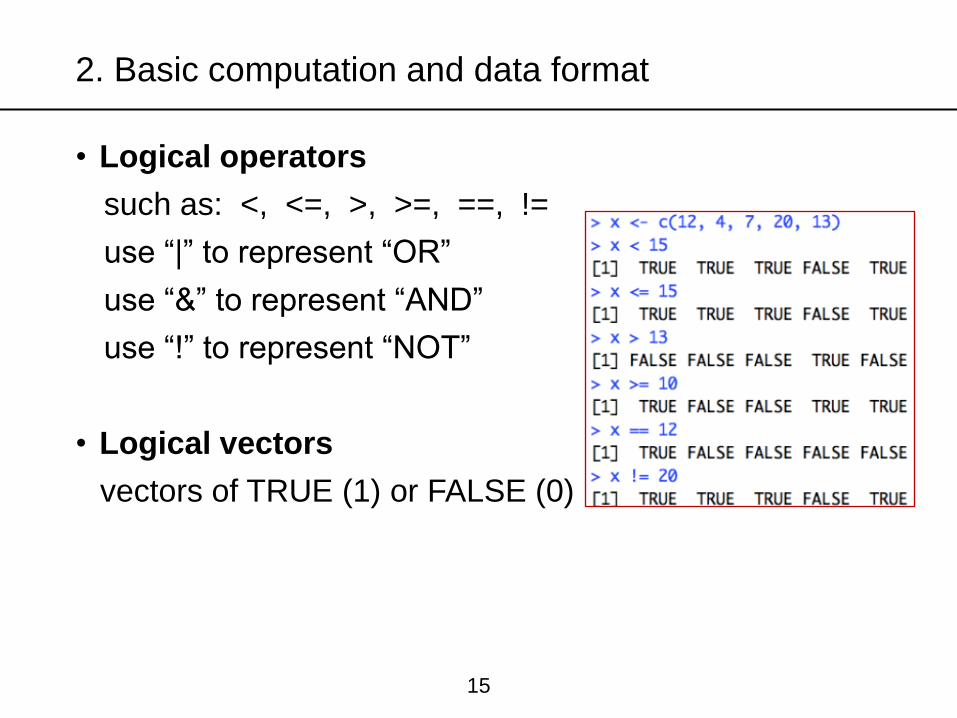
• Logical operators
such as: <, <=, >, >=, ==, !=
use “|” to represent “OR”
use “&” to represent “AND”
use “!” to represent “NOT”
• Logical vectors
vectors of TRUE (1) or FALSE (0)
2. Basic computation and data format
15
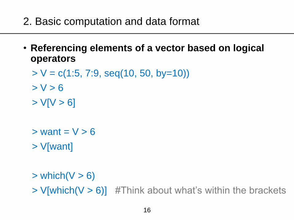
• Referencing elements of a vector based on logical operators
> V = c(1:5, 7:9, seq(10, 50, by=10))
> V > 6
> V[V > 6]
> want = V > 6
> V[want]
> which(V > 6)
> V[which(V > 6)] #Think about what’s within the brackets
2. Basic computation and data format
16
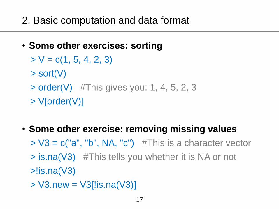
• Some other exercises: sorting
> V = c(1, 5, 4, 2, 3)
> sort(V)
> order(V) #This gives you: 1, 4, 5, 2, 3
> V[order(V)]
• Some other exercise: removing missing values
> V3 = c("a", "b", NA, "c") #This is a character vector
> is.na(V3) #This tells you whether it is NA or not
>!is.na(V3)
> V3.new = V3[!is.na(V3)]
2. Basic computation and data format
17
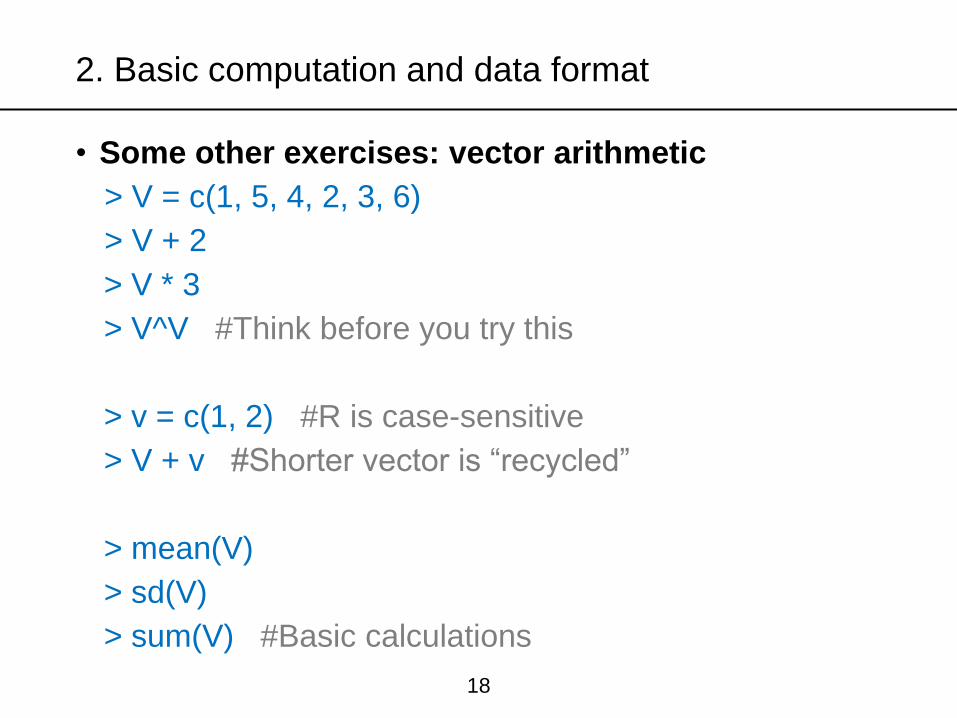
• Some other exercises: vector arithmetic
> V = c(1, 5, 4, 2, 3, 6)
> V + 2
> V * 3
> V^V #Think before you try this
> v = c(1, 2) #R is case-sensitive
> V + v #Shorter vector is “recycled”
> mean(V)
> sd(V)
> sum(V) #Basic calculations
2. Basic computation and data format
18
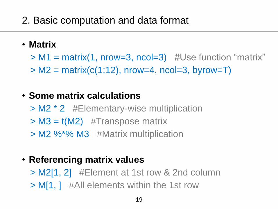
• Matrix
> M1 = matrix(1, nrow=3, ncol=3) #Use function “matrix”
> M2 = matrix(c(1:12), nrow=4, ncol=3, byrow=T)
• Some matrix calculations
> M2 * 2 #Elementary-wise multiplication
> M3 = t(M2) #Transpose matrix
> M2 %*% M3 #Matrix multiplication
• Referencing matrix values
> M2[1, 2] #Element at 1st row & 2nd column
> M[1, ] #All elements within the 1st row
2. Basic computation and data format
19
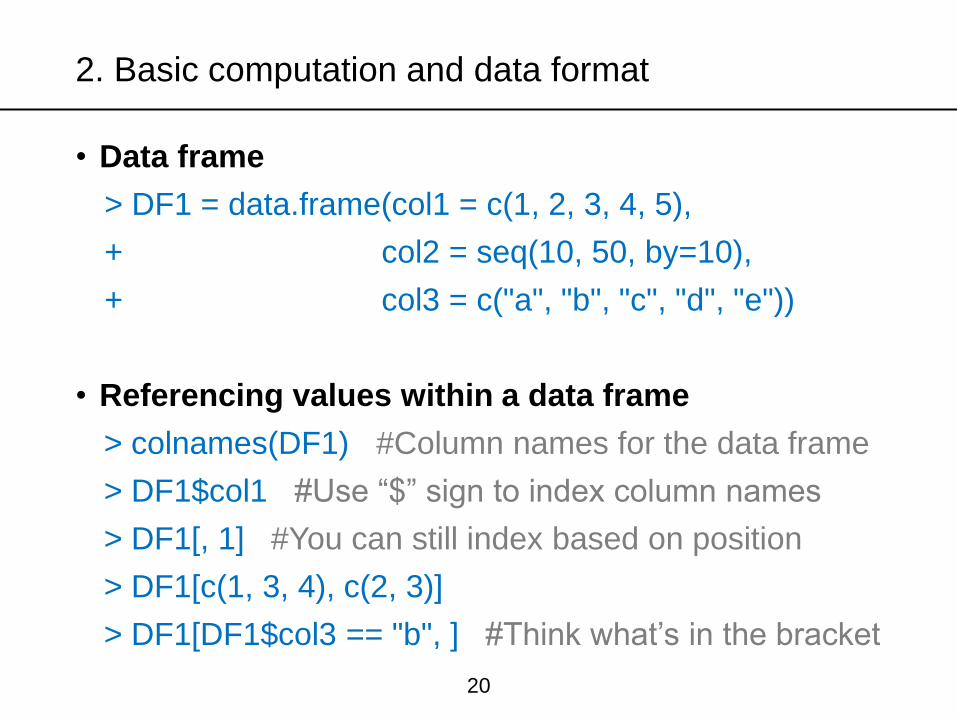
• Data frame
> DF1 = data.frame(col1 = c(1, 2, 3, 4, 5),
+ col2 = seq(10, 50, by=10),
+ col3 = c("a", "b", "c", "d", "e"))
• Referencing values within a data frame
> colnames(DF1) #Column names for the data frame
> DF1$col1 #Use “$” sign to index column names
> DF1[, 1] #You can still index based on position
> DF1[c(1, 3, 4), c(2, 3)]
> DF1[DF1$col3 == "b", ] #Think what’s in the bracket
2. Basic computation and data format
20
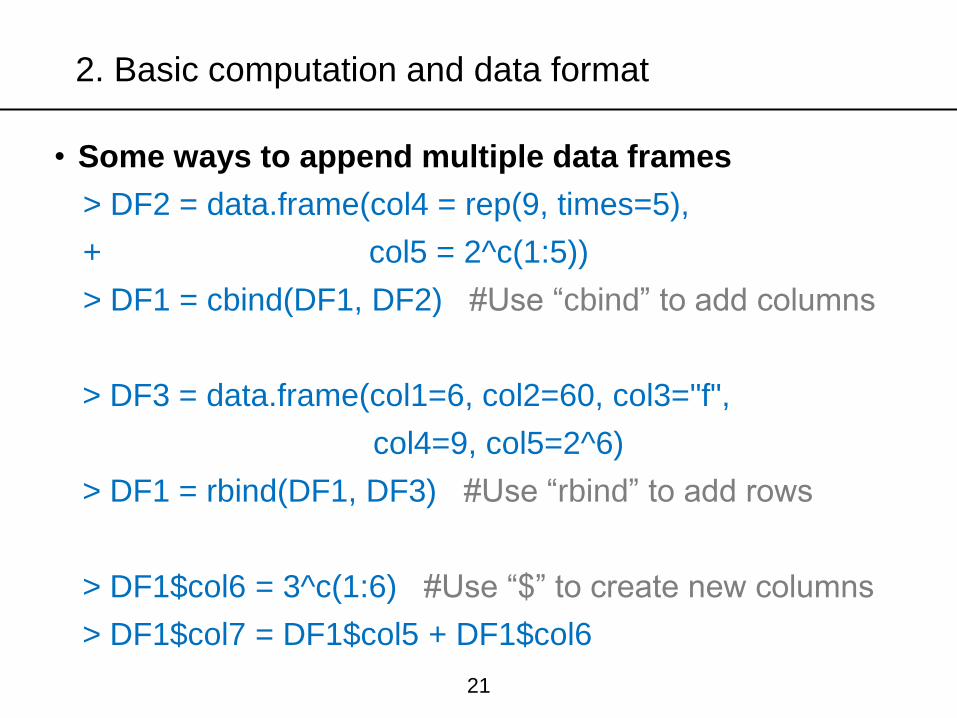
• Some ways to append multiple data frames
> DF2 = data.frame(col4 = rep(9, times=5),
+ col5 = 2^c(1:5))
> DF1 = cbind(DF1, DF2) #Use “cbind” to add columns
> DF3 = data.frame(col1=6, col2=60, col3="f",
col4=9, col5=2^6)
> DF1 = rbind(DF1, DF3) #Use “rbind” to add rows
> DF1$col6 = 3^c(1:6) #Use “$” to create new columns
> DF1$col7 = DF1$col5 + DF1$col6
2. Basic computation and data format
21
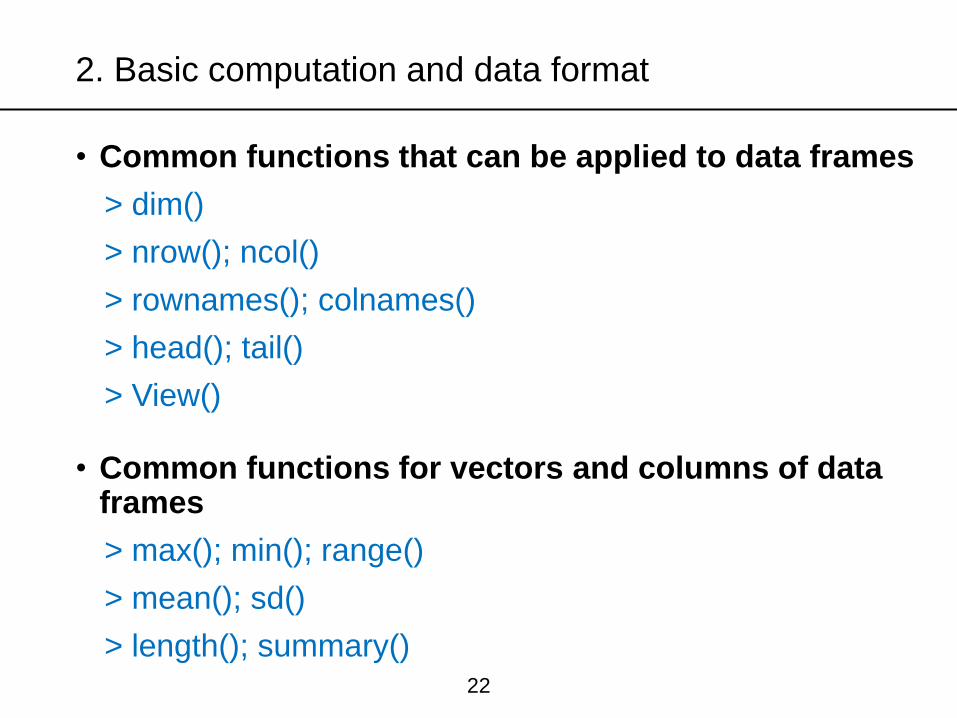
• Common functions that can be applied to data frames
> dim()
> nrow(); ncol()
> rownames(); colnames()
> head(); tail()
> View()
• Common functions for vectors and columns of data frames
> max(); min(); range()
> mean(); sd()
> length(); summary()
2. Basic computation and data format
22
23
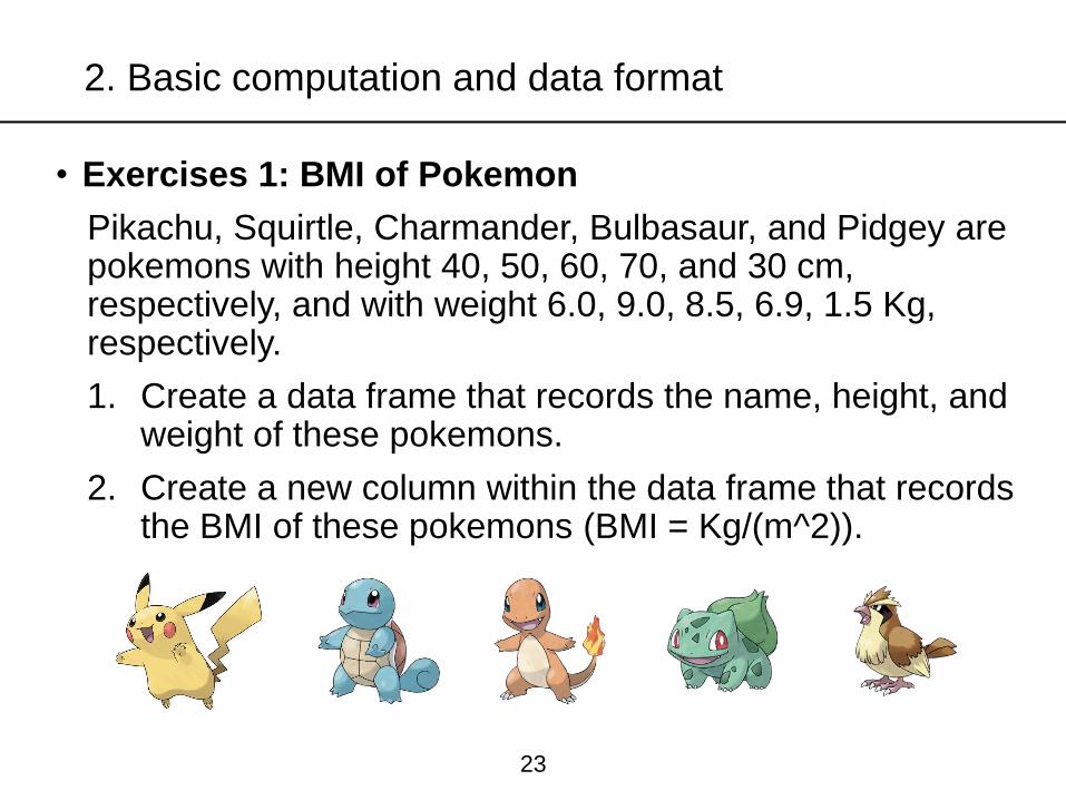
• Exercises 1: BMI of Pokemon
Pikachu, Squirtle, Charmander, Bulbasaur, and Pidgey are pokemons with height 40, 50, 60, 70, and 30 cm, respectively, and with weight 6.0, 9.0, 8.5, 6.9, 1.5 Kg, respectively.
1. Create a data frame that records the name, height, and weight of these pokemons.
2. Create a new column within the data frame that records the BMI of these pokemons (BMI = Kg/(m^2)).
2. Basic computation and data format
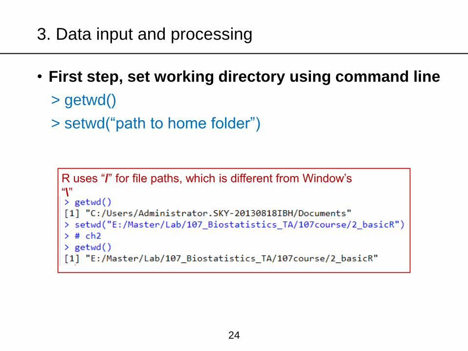
• First step, set working directory using command line
> getwd()
> setwd(“path to home folder”)
3. Data input and processing
24
R uses “/” for file paths, which is different from Window’s
“\”
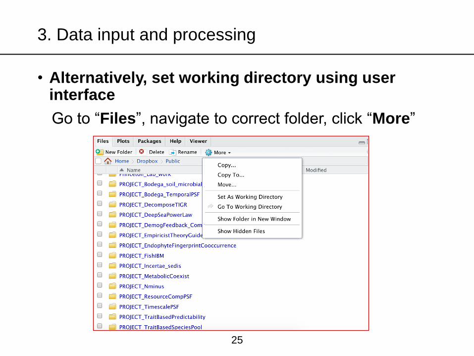
• Alternatively, set working directory using user interface
Go to “Files”, navigate to correct folder, click “More”
3. Data input and processing
25
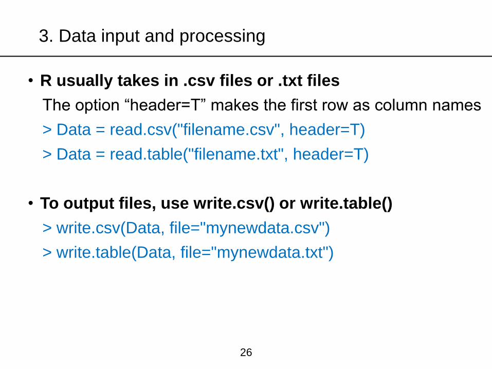
• R usually takes in .csv files or .txt files
The option “header=T” makes the first row as column names
> Data = read.csv("filename.csv", header=T)
> Data = read.table("filename.txt", header=T)
• To output files, use write.csv() or write.table()
> write.csv(Data, file="mynewdata.csv")
> write.table(Data, file="mynewdata.txt")
3. Data input and processing
26
• Exercise 2: read in data files and perform data screening
1. Set you local folder as the working directory, read in the file “example_dat.txt” and save it with the name “data”.
2. Inspect the data with commands mentioned in previous sections, e.g., summary(), head(), dim().
3. Chl.a shouldn’t be negative! Create a new data named “data_new” with those rows removed.
4. Look up the function “apply” using ?apply. Use the function to calculate the mean of all environment variables (i.e., columns 3-9).
3. Data input and processing
27
• Common plotting commands
plot(x, y, data)
plot(y~x, data)
hist(x) (Histogram)
barplot() (Barplot)
boxplot() (Boxplot)
• Plot one single variable using “plot(x)”
> plot(data_new$Chl.a.)
4. Data visualization and plotting
28
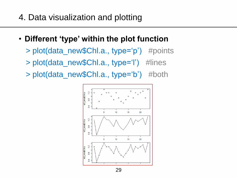
• Different ‘type’ within the plot function
> plot(data_new$Chl.a., type=‘p’) #points
> plot(data_new$Chl.a., type=‘l’) #lines
> plot(data_new$Chl.a., type=‘b’) #both
4. Data visualization and plotting
29
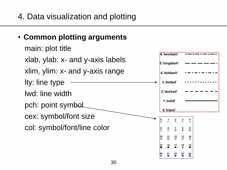
• Common plotting arguments
main: plot title
xlab, ylab: x- and y-axis labels
xlim, ylim: x- and y-axis range
lty: line type
lwd: line width
pch: point symbol
cex: symbol/font size
col: symbol/font/line color
4. Data visualization and plotting
30
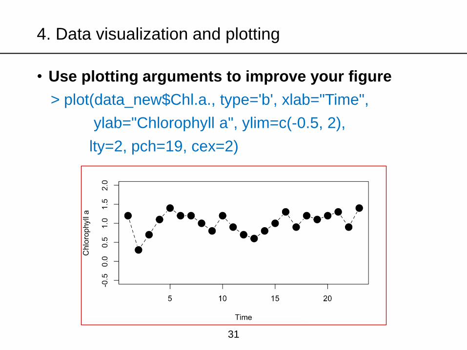
• Use plotting arguments to improve your figure
> plot(data_new$Chl.a., type='b', xlab="Time",
ylab="Chlorophyll a", ylim=c(-0.5, 2),
lty=2, pch=19, cex=2)
4. Data visualization and plotting
31
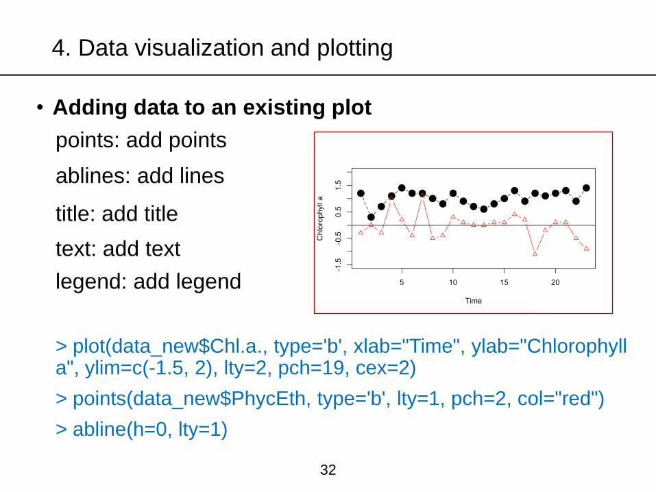
• Adding data to an existing plot
points: add points
ablines: add lines
title: add title
text: add text
legend: add legend
> plot(data_new$Chl.a., type='b', xlab="Time", ylab="Chlorophyll a", ylim=c(-1.5, 2), lty=2, pch=19, cex=2)
> points(data_new$PhycEth, type='b', lty=1, pch=2, col="red")
> abline(h=0, lty=1)
4. Data visualization and plotting
32
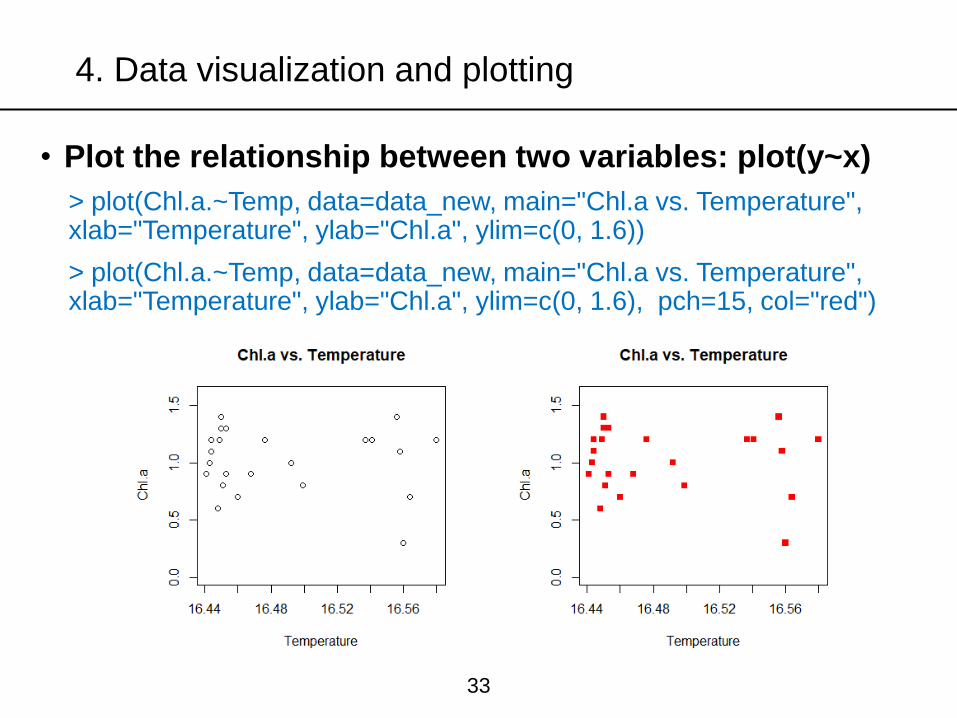
• Plot the relationship between two variables: plot(y~x)
> plot(Chl.a.~Temp, data=data_new, main="Chl.a vs. Temperature", xlab="Temperature", ylab="Chl.a", ylim=c(0, 1.6))
> plot(Chl.a.~Temp, data=data_new, main="Chl.a vs. Temperature", xlab="Temperature", ylab="Chl.a", ylim=c(0, 1.6), pch=15, col="red")
4. Data visualization and plotting
33
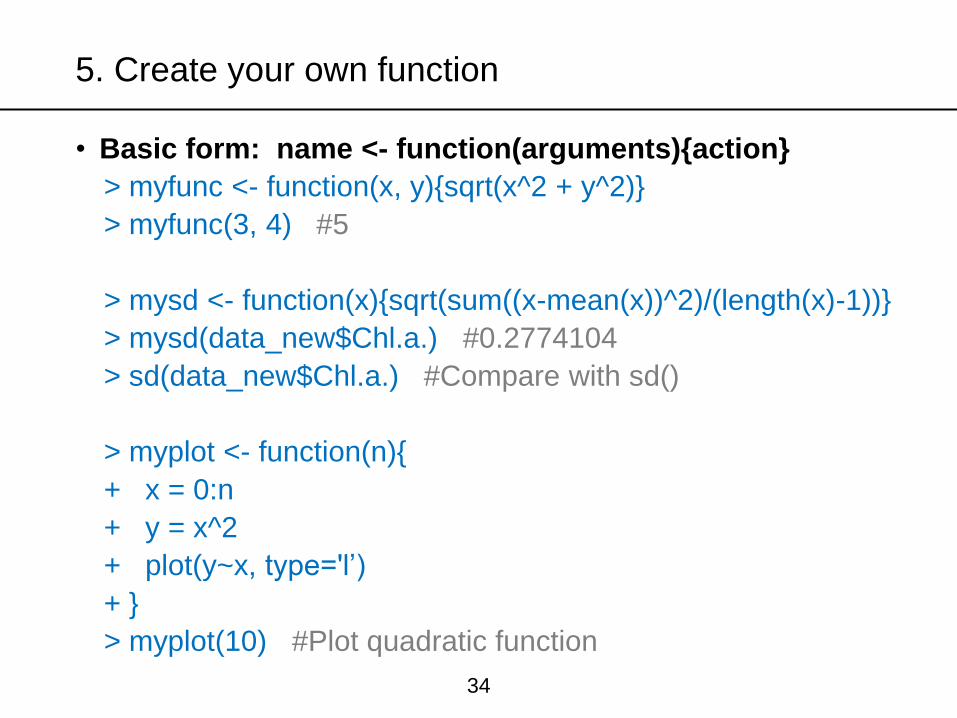
• Basic form: name <- function(arguments){action}
> myfunc <- function(x, y){sqrt(x^2 + y^2)}
> myfunc(3, 4) #5
> mysd <- function(x){sqrt(sum((x-mean(x))^2)/(length(x)-1))}
> mysd(data_new$Chl.a.) #0.2774104
> sd(data_new$Chl.a.) #Compare with sd()
> myplot <- function(n){
+ x = 0:n
+ y = x^2
+ plot(y~x, type='l’)
+ }
> myplot(10) #Plot quadratic function
5. Create your own function
34
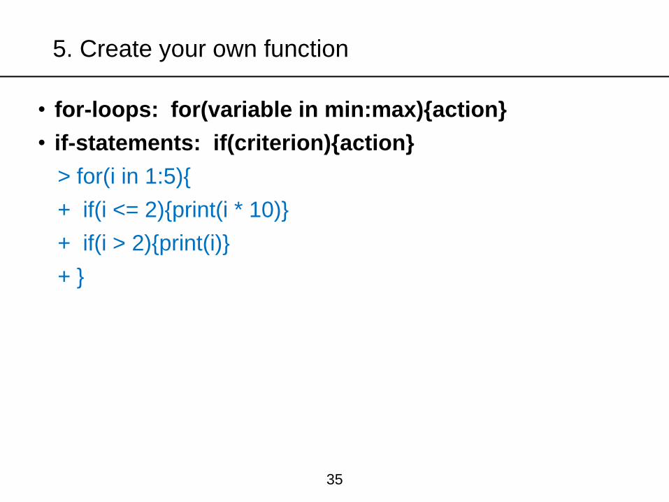
• for-loops: for(variable in min:max){action}
• if-statements: if(criterion){action}
> for(i in 1:5){
+ if(i <= 2){print(i * 10)}
+ if(i > 2){print(i)}
+ }
5. Create your own function
35
• Exercise 3: classifying data based on values
Add a new column in the data data_new, named “category”. The value of this column is 1 if turbidity is less than 10, 2 if between 10 to 15, and 3 if turbidity is greater than 15
5. Create your own function
36