Introduction to Wavelets and Wavelet Transforms

A Primer

C. Sidney Burrus, Ramesh A. Gopinath, and .Haitao Guo

with additional material and programs by

. Jan E. Odegard and Ivan W. Selesnick

Electrical and Computer Engineering Department and Computer and Information Technology Institute

Rice University Houston, Texas

csb@rice.edu

Prentice Hall Upper Saddle River, New Jersey 07458

Library of Congress Cata.loging-in-Publication Data

BURRUS, C. S. Introduction to wavelets and wavelet transforms : a primer / C.

Sidney Burrus, Ramesh A. Gopinath, and Haitao Guo ; with additional material and programs by Jan E. Odegard and Ivan W. Selesnick.

p. em. Includes bibliographical references and index. ISBN 0-13-489600-9 1. Wavelets (Mathematics) I. Gopinath, Ramesh A. QA403.3.B87 1998

2. Signal processing-Mathematics. II. Guo, Haitao. III. Title.

515' .2433-DC21

Acquisitions Editor: Tom Robbins Production Editor: Sharyn Vitrano Editor-in-Chief Marcia Horton Managing Editor: Bayani Mendoza DeLeon Copy Editor: Irwin Zucker

97-53263 CIP

paver Designer: Bruce K enselaar Director of Production and Manufacturing: David W. Riccardi Manufacturing Buyer: Donna Sullivan Editorial Assistant: Nancy Garcia Composition: PRE!EX, INC.

© 1998 by Prentice-Hall, Inc. Simon & Schuster / A Viacom Company Upper Saddle River, New Jersey 07458

The author and publisher of this book have used their best efforts in preparing this book. These efforts include the development, research, and testing of the theories and programs to determine their effectiveness. The author and publisher make no warranty of any kind, expressed or implied, witb regard to these programs or the documentation contained in this book. The author and publisher shall not be liable in any event for incidental or. consequential damages in connection with, or arising out of, the furnishing, performance, or use of these programs.

All rights reserved. No part of this book may be reproduced, in any form or by any means, without permission in writing from the publisher.

Printed in the United States of America

10 9 8 7 6 5 4 3 2 1

ISBN 0-13-489600-9

Prentice-Hall International (UK) Limited, London Prentice-Hall of Australia Pty. Limited, Sydney Prentice-Hall Canada Inc., Toronto Prentice-Hall Hispanoamericana, S.A., Mexico Prentice-Hall of India Private Limited, New Delhi Prentice-Hall of Japan, Inc., Tokyo Simon & Schuster Asia Pte. Ltd., Singapore Editora Prentice-Hall do Brasil, Ltda., Rio de Janeiro

To

Virginia Burrus and Charles Burrus,

Kalyani Narasimhan,

Yongtai Guo and Caijie Li

Contents

Preface

1 Introduction to Wavelets 1.1 Wavelets and Wavelet Expansion Systems

What is a Wavelet Expansion or a Wavelet Transform? What is a Wavelet System? More Specific Characteristics of Wavelet Systems Haar Scaling Functions and Wavelets What do Wavelets Look Like? Why is Wavelet Analysis Effective?

1.2 The Discrete Wavelet Transform 1.3 The Discrete-Time and Continuous Wavelet Transforms 1.4 Exercises and Experiments 1.5 This Chapter

2 A Multiresolution Formulation of Wavelet Systems 2.1 Signal Spaces 2.2 The Scaling Function

Multiresolution Analysis 2.3 The Wavelet Functions 2.4 The Discrete Wavelet Transform 2.5 A Parseval's Theorem 2.6 Display of the Discrete Wavelet Transform and the Wavelet Expansion 2. 7 Examples of Wavelet Expansions 2.8 An Example of the Haar Wavelet System

3 Filter Banks and the Discrete Wavelet Transform 3.1 Analysis - From Fine Scale to Coarse Scale

Filtering and Down-Sampling or Decimating 3.2 Synthesis -From Coarse Scale to Fine Scale

Filtering and Up-Sampling or Stretching 3.3 Input Coefficients 3.4 Lattices and Lifting

xi

1 2 2 2 3 5 5 6 7 8 9 9

10 10 11 12 14 17 18 18 20 23

31 31 32 36 36 37 38

v

vi Contents

3.5 Different Points of View 38 Multiresolution versus Time-Frequency Analysis 38 Periodic versus Nonperiodic Discrete Wavelet Transforms 38 The Discrete Wavelet Transform versus the Discrete-Time Wavelet Transform 39 Numerical Complexity of the Discrete Wavelet Transform 40

4 Bases, Orthogonal Bases, Biorthogonal Bases, Frames, Tight Frames, and U n-conditional Bases 41 4.1 Bases, Orthogonal Bases, and Biorthogonal Bases 41

Matrix Examples 43 Fourier Series Example 44 Sine Expansion Example 44

4.2 Frames and Tight Frames 45 Matrix Examples 46 Sine Expansion as a Tight Frame Example 47

4.3 Conditional and Unconditional Bases 48

5 The Scaling Function and Scaling Coefficients, Wavelet and Wavelet Coeffi­cients 5.1 Tools and Definitions

Signal Classes Fourier Transforms Refinement and Transition Matrices

5.2 Necessary Conditions 5.3 Frequency Domain Necessary Conditions 5.4 Sufficient Conditions

Wavelet System Design 5.5 The Wavelet 5.6 Alternate Normalizations 5. 7 Example Scaling Functions and Wavelets

Haar Wavelets Sine Wavelets Spline and Battle-Lemarie Wavelet Systems

5.8 Further Properties of the Scaling Function and Wavelet General Properties not Requiring Orthogonality Properties that Depend on Orthogonality

5.9 Parameterization of the Scaling Coefficients Length-2 Scaling Coefficient Vector Length-4 Scaling Coefficient Vector Length-6 Scaling Coefficient Vector

5.10 Calculating the Basic Scaling Function and Wavelet Successive Approximations or the Cascade Algorithm Iterating the Filter Bank Successive approximations in the frequency domain The Dyadic Expansion of the Scaling Function

50 50 50 51 52 53 54 56 57 58 59 59 60 60 62 62 63 64 65 65 66 66 67 67 68 68 70

CONTENTS

6 Regularity, Moments, and Wavelet System Design 6.1 K-Regular Scaling Filters 6.2 Vanishing Wavelet Moments 6.3 Daubechies' Method for Zero Wavelet Moment Design 6.4 Non-Maximal Regularity Wavelet Design 6.5 Relation of Zero Wavelet Moments to Smoothness 6.6 Vanishing Scaling Function Moments 6. 7 Approximation of Signals by Scaling Function Projection 6.8 Approximation of Scaling Coefficients by Samples of the Signal 6.9 Coiflets and Related Wavelet Systems

Generalized Coifman Wavelet Systems 6.10 Minimization of Moments Rather than Zero Moments

7 Generalizations of the Basic Multiresolution Wavelet System 7.1 Tiling the Time-Frequency or Time-Scale Plane

Nonstationary Signal Analysis Tiling with the Discrete-Time Short-Time Fourier Transform Tiling with the Discrete Two-Band Wavelet Transform General Tiling

7.2 Multiplicity-M (M-Band) Scaling Functions and Wavelets Properties of M-Band Wavelet Systems M-Band Scaling Function Design M-Band Wavelet Design and Cosine Modulated Methods

7.3 Wavelet Packets

vii

73 73 75 76 83 83 86 86 87 88 93 97

98 98 99

100 100 101 102 103 109 110 110

Full Wavelet Packet Decomposition 110 Adaptive Wavelet Packet Systems 111

7.4 Biorthogonal Wavelet Systems 114 Two-Channel Biorthogonal Filter Banks 114 Biorthogonal Wavelets 116 Comparisons of Orthogonal and Biorthogonal Wavelets 117 Example Families of Biorthogonal Systems 118 Cohen-Daubechies-Feauveau Family of Biorthogonal Spline Wavelets 118 Cohen-Daubechies-Feauveau Family of Biorthogonal Wavelets with Less Dissimilar

Filter Length 118 Tian-Wells Family of Biorthogonal Coiflets 119 Lifting Construction of Biorthogonal Systems 119

7.5 Multiwavelets 122 Construction of Two-Band Multiwavelets Properties of Multiwavelets Approximation, Regularity and Smoothness Support Orthogonality Implementation of Multiwavelet Transform Examples Geronimo-Hardin-Massopust M ul tiwavelets Spline Multiwavelets

123 124 124 124 125 125 126 126 127

viii Contents

Other Constructions 127 Applications 128

7.6 Overcomplete Representations, Frames, Redundant Transforms, and Adaptive Bases128 Overcomplete Representations 129 A Matrix Example 129 Shift-Invariant Redundant Wavelet Transforms and Nondecimated Filter Banks 132 Adaptive Construction of Frames and Bases 133

7. 7 Local Trigonometric Bases 134 Nonsmooth Local Trigonometric Bases 136 Construction of Smooth Windows, 136 Folding and Unfolding 137 Local Cosine and Sine Bases 139 Signal Adaptive Local Trigonometric Bases 141

7.8 Discrete Multiresolution Analysis, the Discrete-Time Wavelet Transform, and the Continuous Wavelet Transform 141 Discrete Multiresolution Analysis and the Discrete-Time Wavelet Transform 143 Continuous Wavelet Transforms 144 Analogies between Fourier Systems and Wavelet Systems

8 Filter Banks and Transmultiplexers 8.1 Introduction

The Filter Bank TransmultiP!,exer Perfect Reconstruction-A Closer Look Direct Characterization of PR Matrix characterization of PR Polyphase (Transform-Domain) Characterization of PR

8.2 Unitary Filter Banks 8.3 Unitary Filter Banks-Some Illustrative Examples 8.4 M-band Wavelet Tight Frames 8.5 Modulated Filter Banks

Unitary Modulated Filter Bank 8.6 Modulated Wavelet Tight Frames 8. 7 Linear Phase Filter Banks

Characterization of Unitary Hp(z) - PS Symmetry Characterization of Unitary Hp(z) - PCS Symmetry Characterization of Unitary Hp(z) -Linear-Phase Symmetry Characterization of Unitary Hp(z) -Linear Phase and PCS Symmetry Characterization of Unitary Hp(z) -Linear Phase and PS Symmetry

8.8 Linear-Phase Wavelet Tight Frames 8.9 Linear-Phase Modulated Filter Banks

DCT /DST 1/11 based 2M Channel Filter Bank 8.10 Linear Phase Modulated Wavelet Tight Frames 8.11 Time-Varying Filter Bank Trees

Growing a Filter Bank Tree Pruning a Filter Bank Tree

145

148 148 148 150 150 150 152 153 155 160 162 164 167 168 169 173 174 174 175 175 176 177 178 178 179 182 182

CONTENTS

Wavelet Bases for the Interval Wavelet Bases for L2 ([0, oo)) Wavelet Bases for L2 ((-oo,O]) Segmented Time-Varying Wavelet Packet Bases

8.12 Filter Banks and Wavelets-Summary

9 Calculation of the Discrete Wavelet Transform 9.1 Finite Wavelet Expansions and Transforms 9.2 Periodic or Cyclic Discrete Wavelet Transform 9.3 Filter Bank Structures for Calculation of th~ DWT and Complexity 9.4 The Periodic Case 9.5 Structure of the Periodic Discrete Wavelet Transform 9.6 More General Structures

10 Wavelet-Based Signal Processing and Applications 10.1 Wavelet-Based Signal Processing 10.2 Approximate FFT using the Discrete Wavelet Transform

Introduction

ix

183 183 184 185 186

188 188 190 191 192 194 195

196 196 197 197

Review of the Discrete Fourier Transform and FFT 198 Review of the Discrete Wavelet Transform 200 The Algorithm Development 201 Computational Complexity 203 Fast Approximate Fourier Transform 203 Computational Complexity 203 Noise Reduction Capacity 204 Summary 204

10.3 Nonlinear Filtering or Denoising with the DWT 205 Denoising by Thresholding 206 Shift-Invariant or Nondecimated Discrete Wavelet Transform 207 Combining the Shensa-Beylkin-Mallat-a trous Algorithms and Wavelet Denoising 209 Performance Analysis 209 Examples of Denoising 210

10.4 Statistical Estimation 211 10.5 Signal and Image Compression 212

Fundamentals of Data Compression 212 Prototype Transform Coder 213 Improved Wavelet Based Compression Algorithms 215

10.6 Why are Wavelets so Useful? 216 10.7 Applications 217

Numerical Solutions to Partial Differential Equations 217 Seismic and Geophysical Signal Processing 217 Medical and Biomedical Signal and Image Processing 218 Application in Communications 218 Fractals 218

10.8 Wavelet Software 218

X

11 Summary Overview 11.1 Properties of the Basic Multiresolution Scaling Function 11.2 Types of Wavelet Systems

12 References

Bibliography

Appendix A. Derivations for Chapter 5 on Scaling Functions

Appendix B. Derivations for Section on Properties

Appendix C. Matlab Programs

Index

Contents

219 219 221

223

224

246

253

258

266

Preface

This book develops the ideas behind and properties of wavelets and shows how they can be used as analytical tools for signal processing, numerical analysis, and mathematical modeling. We try to present this in a way that is accessible to the engineer, scientist, and applied mathematician both as a theoretical approach and as a potentially practical method to solve problems. Although the roots of this subject go back some time, the modern interest and development have a history of only a few years.

The early work was in the 1980's by Morlet, Grossmann, Meyer, Mallat, and others, but it was the paper by Ingrid Daubechies [Dau88a] in 1988 that caught the attention of the larger applied mathematics communities in signal processing, statistics, and numerical analysis. Much of the early work took place in France [CGT89, Mey92a] and the USA [Dau88a, RBC*92, Dau92, RV91]. As in many new disciplines, the first work was closely tied to a particular application or traditional theoretical framework. Now we are seeing the theory abstracted from application and developed on its own and seeing it related to other parallel ideas. Our own background and interests in signal processing certainly influence the presentation of this book.

The goal of most modern wavelet research is to create a set of basis functions (or general expansion functions) and transforms that will give an informative, efficient, and useful description of a function or signal. If the signal is represented as a function of time, wavelets provide efficient localization in both time and frequency or scale. Another central idea is that of multiresolution where the decomposition of a signal is in terms of the resolution of detail.

For the Fourier series, sinusoids are chosen as basis functions, then the properties of the resulting expansion are examined. For wavelet analysis, one poses the desired properties and then derives the resulting basis functions. An important property of the wavelet basis is providing a multiresolution analysis. For several reasons, it is often desired to have the basis functions orthonormal. Given these goals, you will see aspects of correlation techniques, Fourier transforms, short-time Fourier transforms, discrete Fourier transforms, Wigner distributions, filter banks, subband coding, and other signal expansion and processing methods in the results.

Wavelet-based analysis is an exciting new problem-solving tool for the mathematician, scien­tist, and engineer. It fits naturally with the digital computer with its basis f)\nctions defined by summations not integrals or derivatives. Unlike most traditional expansion systems, the basis functions of the wavelet analysis are not solutions of differential equations. In some areas, it is the first truly new tool we have had in many years. Indeed, use of wavelets and wavelet transforms requires a new point of view and a new method of interpreting representations that we are still learning how to exploit.

xi

xii Preface

More recently, work by Donoho, Johnstone, Coifman, and others have added theoretical reasons for why wavelet analysis is so versatile and powerful, and have given generalizations that are still being worked on. They have shown that wavelet systems have some inherent generic advantages and are near optimal for a wide class of problems [Don93b]. They also show that adaptive means can create special wavelet systems for particular signals and classes of signals.

The multiresolution decomposition seems to separate components of a signal in a way that is superior to most other methods for analysis, processing, or compression. Because of the ability of the discrete wavelet transform to decompose a signal at different independent scales and to do it in a very flexible way, Burke calls wavelets "The Mathematical Microscope" [Bur94, Hub96]. Because of this powerful and flexible decomposition, linear and nonlinear processing of signals in the wavelet transform domain offers new methods for signal detection, filtering, and compression [Don93b, Don95, Don93a, Sai94b, WTWB97, Guo97]. It also can be used as the basis for robust numerical algorithms.

You will also see an interesting connection and equivalence to filter bank theory from digital signal processing [Vai92, AH92]. Indeed, some of the results obtained with filter banks are the same as with discrete-time wavelets, and this has been developed in the signal processing community by Vetterli, Vaidyanathan, Smith and Barnwell, and others. Filter banks, as well as most algorithms for calculating wavelet transforms, are part of a still more general area of multirate and time-varying systems.

The presentation here will be as a tutorial or primer for people who know little or nothing about wavelets but do have a technical background. It assumes a knowledge of Fourier series and transforms and of linear algebra and matrix theory. It also assumes a background equivalent to a B.S. degree in engineering, science, or applied mathematics. Some knowledge of signal processing is helpful but not essential. We develop the ideas in terms of one-dimensional signals [RV91] modeled as real or perhaps complex functions of time, but the ideas and methods have also proven effective in image representation and processing [SA92, Mal89a] dealing with two, three, or even four dimensions. Vector spaces have proved to be a natural setting for developing both the theory and applications of wavelets. Some background in that area is helpful but can be picked up as needed. The study and understanding of wavelets is greatly assisted by using some sort of wavelet software system to work out examples and run experiments. MATLAB™ programs are included at the end of this book and on our web site (noted at the end of the preface). Several other systems are mentioned in Chapter 10.

There are several different approaches that one could take in presenting wavelet theory. We have chosen to start with the representation of a signal or function of continuous time in a series expansion, much as a Fourier series is used in a Fourier analysis. From this series representation, we can move to the expansion of a function of a discrete variable (e.g., samples of a signal) and the theory of filter banks to efficiently calculate and interpret the expansion coefficients. This would be analogous to the discrete Fourier transform (DFT) and its efficient implementation, the fast Fourier transform (FFT). We can also go from the series expansion to an integral transform called the continuous wavelet transform, which is analogous to the Fourier transform or Fourier integral. We feel starting with the series expansion gives the greatest insight and provides ease in seeing both the similarities and differences with Fourier analysis.

This book is organized into sections and chapters, each somewhat self-contained. The earlier chapters give a fairly complete development of the discrete wavelet transform (DWT) as a series expansion of signals in terms of wavelets and scaling functions. The later chapters are short descriptions of generalizations of the DWT and of applications. They give references to other

Preface xiii

works, and serve as a sort of annotated bibliography. Because we intend this book as an intro­duction to wavelets which already have an extensive literature, we have included a rather long bibliography. However, it will soon be incomplete because of the large number of papers that are currently being published. Nevertheless, a guide to the other literature is essential to our goal of an introduction.

A good sketch of the philosophy of wavelet analysis and the history of its development can be found in a recent book published by the National Academy of Science in the chapter by Barbara Burke [Bur94]. She has written an excellent expanded version in [Hub96], which should be read by anyone interested in wavelets. Daubechies gives a brief history of the early research in [Dau96].

Many of the results and relationships presented in this book are in the form of theorems and proofs or derivations. A real effort has been made to ensure the correctness of the statements of theorems but the proofs are often only outlines of derivations intended to give insight into the result rather than to be a formal proof. Indeed, many of the derivations are put in the Appendix in order not to clutter the presentation. We hope this style will help the reader gain insight into this very interesting but sometimes obscure new mathematical signal processing tool.

We use a notation that is a mixture of that used in the signal processing literature and that in the mathematical literature. We hope this will make the ideas and results more accessible, but some uniformity and cleanness is lost.

The authors acknowledge AFOSR, ARPA, NSF, Nortel, Inc., Texas Instruments, Inc. and Aware, Inc. for their support of this work. We specifically thank H. L. Resnikoff, who first introduced us to wavelets and who proved remarkably accurate in predicting their power and success. We also thank W. M. Lawton, R. 0. Wells, Jr., R. G. Baraniuk, J. E. Odegard, I. W. Selesnick, M. Lang, J. Tian, and members of the Rice Computational Mathematics Laboratory for many of the ideas and results presented in this book. The first named author would like to thank the Maxfield and Oshman families for their generous support. The students in EE-531 and EE-696 at Rice University provided valuable feedback as did Bruce Francis, Strela Vasily, Hans Schussler, Peter Steffen, Gary Sitton, Jim Lewis, Yves Angel, Curt Michel, J. H. Husoy, Kjersti Engan, Ken Castleman, Jeff Trinkle, Katherine Jones, and other colleagues at Rice and elsewhere.

We also particularly want to thank Tom Robbins and his colleagues at Prentice Hall for their support and help. Their reviewers added significantly to the book.

We would appreciate learning of any errors or misleading statements that any readers dis­cover. Indeed, any suggestions for improvement of the book would be most welcome. Send suggestions or comments via email to csb@rice.edu. Software, articles, errata for this book, and other information on the wavelet research at Rice can be found on the world-wide-web URL: http://www-dsp.rice.edu/ with links to other sites where wavelet research is being done.

C. Sidney Burrus, Ramesh A. Gopinath, and Haitao Guo Houston, Texas, Yorktown Heights, New York, and Sunnyvale, California

xiv Preface

Instructions to the Reader

Although this book in arranged in a somewhat progressive order, starting with basic ideas and definitions, moving to a rather complete discussion of the basic wavelet system, and then on to generalizations, one should skip around when reading or studying from it. Depending on the background of the reader, he or she should skim over most of the book first, then go back and study parts in detail. The Introduction at the beginning and the Summary at the end should be continually consulted to gain or keep a perspective; similarly for the Table of Contents and Index. The MATLAB programs in the Appendix or the Wavelet Toolbox from Mathworks or other wavelet software should be used for continual experimentation. The list of references should be used to find proofs or detail not included here or to pursue research topics or applications. The theory and application of wavelets are still developing and in a state of rapid growth. We hope this book will help open the door to this fascinating new subject.

Chapter 1

Introduction to Wavelets

This chapter will provide an overview of the topics to be developed in the book. Its purpose is to pres~nt the ideas, goals, and outline of properties for an understanding of and ability to use wavelets and wavelet transforms. The details and more careful definitions are given later in the book.

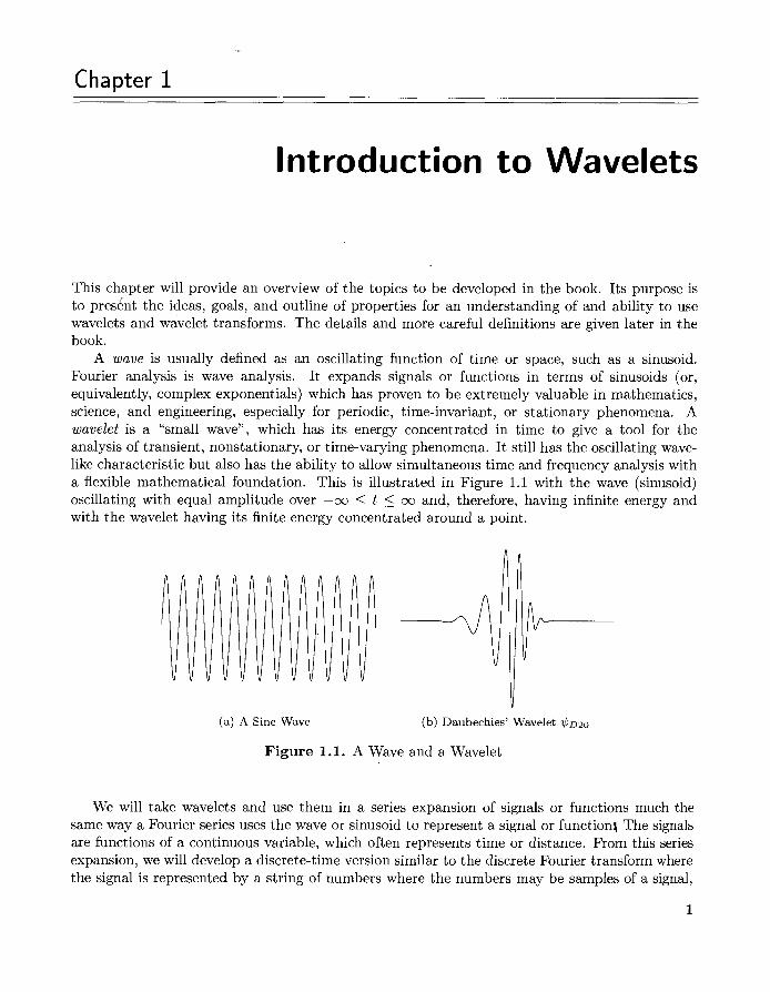
A wave is usually defined as an oscillating function of time or space, such as a sinusoid. Fourier analysis is wave analysis. It expands signals or functions in terms of sinusoids (or, equivalently, complex exponentials) which has proven to be extremely valuable in mathematics, science, and engineering, especially for periodic, time-invariant, or stationary phenomena. A wavelet is a "small wave", which has its energy concentrated in time to give a tool for the analysis of transient, nonstationary, or time-varying phenomena. It still has the oscillating wave­like characteristic but also has the ability to allow simultaneous time and frequency analysis with a flexible mathematical foundation. This is illustrated in Figure 1.1 with the wave (sinusoid) oscillating with equal amplitude over -oo ::::; t ::::; oo and, therefore, having infinite energy and with the wavelet having its finite energy concentrated around a point.

(a) A Sine Wave (b) Daubechies' Wavelet 'I/Jv2o

Figure 1.1. A Wave and a Wavelet

We will take wavelets and use them in a series expansion of signals or functions much the same way a Fourier series uses the wave or sinusoid to represent a signal or function\ The signals are functions of a continuous variable, which often represents time or distance. From this series expansion, we will develop a discrete-time version similar to the discrete Fourier transform where the signal is represented by a string of numbers where the numbers may be samples of a signal,

1

2 Introduction to Wavelets and Transforms Ch. 1

samples of another string of numbers, or inner products of a signal with some expansion set. Finally, we will briefly describe the continuous wavelet transform where both the signal and the transform are functions of continuous variables. This is analogous to the Fourier transform.

1.1 Wavelets and Wavelet Expansion Systems

Before delving into the details of wavelets and their properties, we need to get some idea of their general characteristics and what we are going to do with them [Swe96b].

What is a Wavelet Expansion or a Wavelet Transform?

A signal or function f(t) can often be better analyzed, described, or processed if expressed as a linear decomposition by

f(t) = La£ 7/Jt(t) (1.1) £

where£ is an integer index for the finite or infinite sum, at are the real-valued expansion coeffi­cients, and 7/Jt(t) are a set of real-valued functions oft called the expansion set. If the expansion (1.1) is unique, the set is called a basis for the class of functions that can be so expressed. If the basis is orthogonal, meaning

(7/Jk(t), 7/Jt(t)) = J 7/Jk(t) 7/Jt(t) dt = 0 k =1- £, (1.2)

then the coefficients can be calculated by the inner product

ak = (f(t), 7/Jk(t)) = J f(t) 7/Jk(t) dt. (1.3)

One can see that substituting (1.1) into (1.3) and using (1.2) gives the single ak coefficient. If the basis set is not orthogonal, then a dual basis set ;fik(t) exists such that using (1.3) with the dual basis gives the desired coefficients. This will be developed in Chapter 2.

For a Fourier series, the orthogonal basis functions 7/Jk(t) are sin(kwot) and cos(kwot) with frequencies of kw0 . For a Taylor's series, the nonorthogonal basis functions are simple monomials tk, and for many other expansions they are various polynomials. There are expansions that use splines and even fractals.

For the wavelet expansion, a two-parameter system is constructed such that (1.1) becomes

t(t) = L: L: aj,k 7/Jj,k(t) k j

(1.4)

where both j and k are integer indices and the 7/Jj,k(t) are the wavelet expansion functions that usually form an orthogonal basis.

The set of expansion coefficients aj,k are called the discrete wavelet transform (DWT) of f(t) and (1.4) is the inverse transform.

What is a Wavelet System?

The wavelet expansion set is not unique. There are many different wavelets systems that can be used effectively, but all seem to have the following three general characteristics [Swe96b].

Sec. 1.1. Wavelets and Wavelet Expansion Systems 3

1. A wavelet system is a set of building blocks to construct or represent a signal or function. It is a two-dimensional expansion set (usually a basis) for some class of one- (or higher) dimensional signals. In other words, if the wavelet set is given by ¢1,k(t) for indices of j, k = 1, 2, · · ·, a linear expansion would be f(t) = Lk Lj a1,k ¢1,k(t) for some set of coefficients aj,k·

2. The wavelet expansion gives a time-frequency localization of the signal. This means most of the energy of the signal is well represented by a few expansion coefficients, aj,k·

3. The calculation of the coefficients from the signal can be done efficiently. It turns out that many wavelet transforms (the set of expansion coefficients) can calculated with O(N) operations. This means the number of floating-point multiplications and additions increase linearly with the length of the signal. More general wavelet transforms require O(N log(N)) operations, the same as for the fast Fourier transform (FFT) [BP85].

Virtually all wavelet systems have these very general characteristics. Where the Fourier series maps a one-dimensional function of a continuous variable into a one-dimensional sequence of coefficients, the wavelet expansion maps it into a two-dimensional array of coefficients. We will see that it is this two-dimensional representation that allows localizing the signal in both time and frequency. A Fourier series expansion localizes in frequency in that if a Fourier series expansion of a signal has only one large coefficient, then the signal is essentially a single sinusoid at the frequency determined by the index of the coefficient. The simple time-domain representation of the signal itself gives the localization in time. If the signal is a simple pulse, the location of that pulse is the localization in time. A wavelet representation will give the location in both time and frequency simultaneously. Indeed, a wavelet representation is much like a musical score where the location of the notes tells when the tones occur and what their frequencies are.

More Specific Characteristics of Wavelet Systems

There are three additional characteristics [Swe96b, Dau92] that are more specific to wavelet expansions.

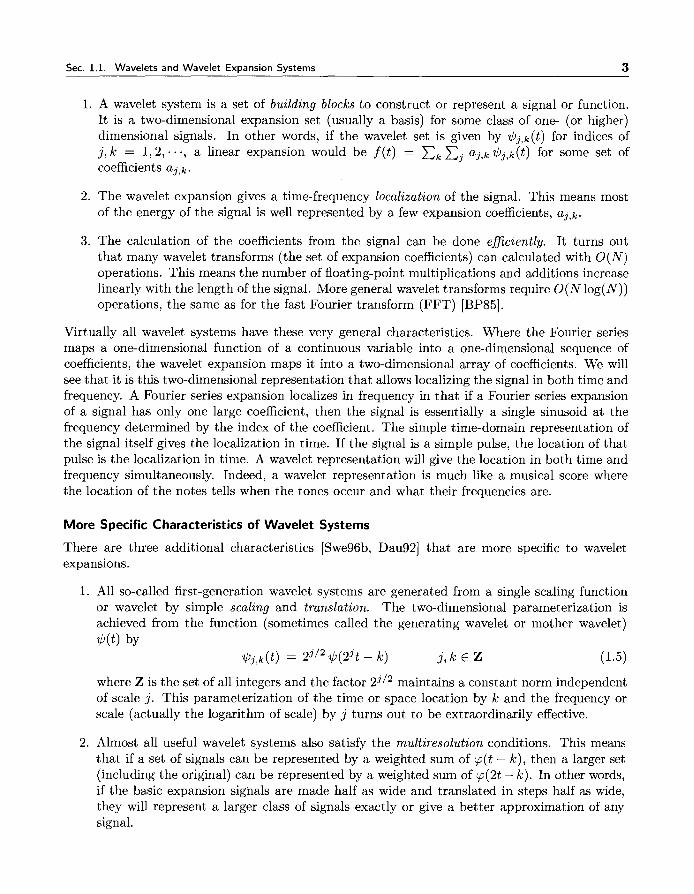
1. All so-called first-generation wavelet systems are generated from a single scaling function or wavelet by simple scaling and translation. The two-dimensional parameterization is achieved from the function (sometimes called the generating wavelet or mother wavelet) 'lj;(t) by

j,k E Z (1.5)

where Z is the set of all integers and the factor 211 2 maintains a constant norm independent of scale j. This parameterization of the time or space location by k and the frequency or scale (actually the logarithm of scale) by j turns out to be extraordinarily effective.

2. Almost all useful wavelet systems also satisfy the multiresolution conditions. This means that if a set of signals can be represented by a weighted sum of cp( t - k), then a larger set (including the original) can be represented by a weighted sum of cp(2t- k ). In other words, if the basic expansion signals are made half as wide and translated in steps half as wide, they will represent a larger class of signals exactly or give a better approximation of any signal.

4 'Introduction to Wavelets and Transforms Ch. 1

3. The lower resolution coefficients can be calculated from the higher resolution coefficients by a tree-structured algorithm called a filter bank. This allows a very efficient calculation of the expansion coefficients (also known as the discrete wavelet transform) and relates wavelet transforms to an older area in digital signal processing.

The operations of translation and scaling seem to be basic to many practical signals and signal­generating processes, and their use is one of the reasons that wavelets are efficient expansion functions. Figure 1.2 is a pictorial representation of the translation and scaling of a single mother wavelet described in (1.5). As the index k changes, the location of the wavelet moves along the horizontal axis. This allows the expansion to explicitly represent the location of events in time or space. As the index j changes, the shape of the wavelet changes in scale. This allows a representation of detail or resolution. Note that as the scale becomes finer (/larger), the steps in time become smaller. It is both the narrower wavelet and the smaller steps that allow representation of greater detail or higher resolution. For clarity, only every fourth term in the translation (k = 1, 5, 9, 13, ···)is shown, otherwise, the figure is a clutter. What is not illustrated here but is important is that the shape of the basic mother wavelet can also be changed. That is done during the design of the wavelet system and allows one set to well-represent a class of signals.

For the Fourier series and transform and for most signal expansion systems, the expansion functions (bases) are chosen, then the properties of the resulting transform are derived and

j

3

2

1 /\ 6

k 1 2 3 4 5 6 7 8

Figure 1. 2. Translation (every fourth k) and Scaling of a Wavelet 7/J D 4

Sec. 1.1. Wavelets and Wavelet Expansion Systems 5

analyzed. For the wavelet system, these properties or characteristics are mathematically required, then the resulting basis functions are derived. Because these constraints do not use all the degrees of freedom, other properties can be required to customize the wavelet system for a particular application. Once you decide on a Fourier series, the sinusoidal basis functions are completely set. That is not true for the wavelet. There are an infinity of very different wavelets that all satisfy the above properties. Indeed, the understanding and design of the wavelets is an important topic of this book.

Wavelet analysis is well-suited to transient signals. Fourier analysis is appropriate for periodic signals or for signals whose statistical characteristics do not change with time. It is the localizing property of wavelets that allow a wavelet expansion of a transient event to be modeled with a small number of coefficients. This turns out to be very-useful in applications.

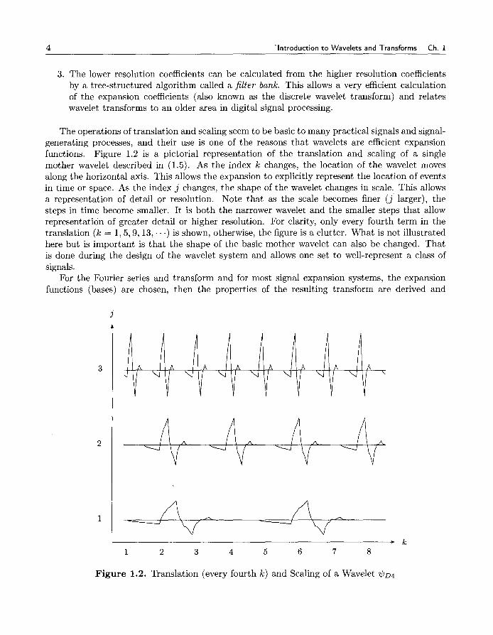
Haar Scaling Functions and Wavelets

The multiresolution formulation needs two closely related basic functions. In addition to the wavelet 'lj;(t) that has been discussed (but not actually defined yet), we will need another basic function called the scaling function cp(t). The reasons for needing this function and the details of the relations will be developed in the next chapter, but here we will simply use it in the wavelet expansion.

The simplest possible orthogonal wavelet system is generated from the Haar scaling function and wavelet. These are shown in Figure 1.3. Using a combination of these scaling functions and wavelets allows a large class of signals to be represented by

00 00 00

f(t) = L Ck cp(t- k) + L L dj,k ¢(2it- k). (1.6) k=-oo k=-ooj=O

Haar [HaalOJ showed this result in 1910, and we now know that wavelets are a generalization of his work. An example of a Haar system and expansion is given at the end of Chapter 2.

( What do Wavelets Look Like?

All Fourier basis functions look alike. A high-frequency sine wave looks like a compressed low­frequency sine wave. A cosine wave is a sine wave translated by 90° or 1r /2 radians. It takes a

0 1 t t

(a) ¢(t) (b) 1/;(t)

Figure 1.3. Haar Scaling Function and Wavelet

6 Introduction to Wavelets and Transforms Ch. 1

large number of Fourier components to represent a discontinuity or a sharp corner. In contrast, there are many different wavelets and some have sharp corners themselves.

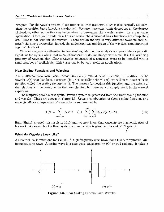
To appreciate the special character of wavelets you should recognize that it was not until the late 1980's that some of the most useful basic wavelets were ever seen. Figure 1.4 illustrates four different scaling functions, each being zero outside of 0 < t < 6 and each generating an orthogonal wavelet basis for all square integrable functions. This figure is also shown on the cover to this book.

Several more scaling functions and their associated wavelets are illustrated in later chapters, and the Haar wavelet is shown in Figure 1.3 and in detail at the end of Chapter 2.

1.5

0.5

0

0 4 5

(a) ¢c6: a= 1.3598,,13 = -0.7821

0.8

0.6

0.4

0.2

0

-0.2 0~--~--~2~--~3~---4~~5

(c) a= ~1r, (3 = -f21l"

1.2

0.8

0.6

0.4

0.2

0

-0.2

-0.4 0 2 3 4 5

(b) tPD6: a= 1.1468,,13 = 0.42403

2

-1

-2

0 2 3 4 5

(d) a= ~1r,,6 = ft1r

Figure 1.4. Example Scaling Functions (See Section 5.8 for the Meaning of a and /3)

Why is Wavelet Analysis Effective?

Wavelet expansions and wavelet transforms have proven to be very efficient and effective in analyzing a very wide class of signals and phenomena. Why is this true? What are the properties that give this effectiveness?

1. The size of the wavelet expansion coefficients aj,k in (1.4) or dj,k in (1.6) drop off rapidly with j and k for a large class of signals. This property is called being an unconditional basis and it is why wavelets are so effective in signal and image compression, denoising, and detection. Donoho [Don93b, DJKP95b] showed that wavelets are near optimal for a wide class of signals for compression, denoising, and detection.

Sec. 1.2. The Discrete Wavelet Transform 7

2. The wavelet expansion allows a more accurate local description and separation of signal characteristics. A Fourier coefficient represents a component that lasts for all time and, therefore, temporary events must be described by a phase characteristic that allows cancel­lation or reinforcement over large time periods. A wavelet expansion coefficient represents a component that is itself local and is easier to interpret. The wavelet expansion may allow a separation of components of a signal that overlap in both time and frequency.

3. Wavelets are adjustable and adaptable. Because there is not just one wavelet, they can be designed to fit individual applications. They are ideal for adaptive systems that adjust themselves to suit the signal.

4. The generation of wavelets and the calculation· of the discrete wavelet transform is well matched to the digital computer. We will later see that the defining equation for a wavelet uses no calculus. There are no derivatives or integrals, just multiplications and additions­operations that are basic to a digital computer.

While some of these details may not be clear at this point, they should point to the issues that are important to both theory and application and give reasons for the detailed development that follows in this and other books.

1.2 The Discrete Wavelet Transform

This two-variable set of basis functions is used in a way similar to the short-time Fourier trans­form, the Gabor transform, or the Wigner distribution for time-frequency analysis [Coh89, Coh95, HB92]. Our goal is to generate a set of expansion functions such that any signal in L2 (R) (the space of square integrable functions) can be represented by the series

or, using (1.5), as

f(t) = L aJ,k 2J/Z '!jJ(2it- k) j,k

f(t) = L aj,k '1/Jj,k(t) j,k

(I. 7)

(1.8)

where the two-dimensional set of coefficients aj,k is called the discrete wavelet transform (DWT) of j(t). A more specific form indicating how the aj,k's are calculated can be written using inner products as

t(t) = L: ('1/JJ,k(t), t(t)) '1/Jj,k(t) j,k

(1.9)

if the '1/Jj,k(t) form an orthonormal basis1 for the space of signals of interest [Dau92]. The inner product is usually defined as

(x(t), y(t)) = J x*(t) y(t) dt. (1.10)

1 Bases and tight frames are defined in Chapter 4.

8 Introduction to Wavelets and Transforms Ch. 1

The goal of most expansions of a function or signal is to have the coefficients of the expansion a1,k give more useful information about the signal than is directly obvious from the signal itself. A second goal is to have most of the coefficients be zero or very small. This is what is called a sparse representation and is extremely important in applications for statistical estimation and detection, data compression, nonlinear noise reduction, and fast algorithms.

Although this expansion is called the discrete wavelet transform (DWT), it probably should be called a wavelet series since it is a series expansion which maps a function of a continuous variable into a sequence of coefficients much the same way the Fourier series does. However, that is not the convention.

This wavelet series expansion is in terms of two indices, the time translation k and the scaling index j. For the Fourier series, there are only two possible values of k, zero and n/2, which give the sine terms and the cosine terms. The values j give the frequency harmonics. In other words, the Fourier series is also a two-dimensional expansion, but that is not seen in the exponential form and generally not noticed in the trigonometric form.

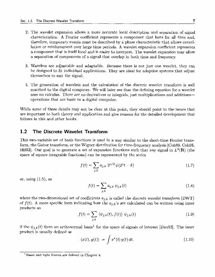
The DWT of a signal is somewhat difficult to illustrate because it is a function of two variables or indices, but we will show the DWT of a simple pulse in Figure 1.5 to illustrate the localization of the transform. Other displays will be developed in the next chapter.

Pulse ------------'

d4(k)

d3(k)

d2(k) I'· 1,.

dl (k) I', I,,

do(k) I

I

co(k) I I I I I I I I I I I I I I I I I I I I

Figure 1.5. Discrete Wavelet Transform of a Pulse, using 'lfJD6 with a Gain of v'2 for Each Higher Scale.

1.3 The Discrete-Time and Continuous Wavelet Transforms

If the signal is itself a sequence of numbers, perhaps samples of some function of a continuous variable or perhaps a set of inner products, the expansion of that signal is called a discrete-time

Sec. 1.4. Exercises and Experiments 9

wavelet transform (DTWT). It maps a sequence of numbers into a sequence of numbers much the same way the discrete Fourier transform (DFT) does. It does not, however, require the signal to be finite in duration or periodic as the DFT does. To be consistent with Fourier terminology, it probably should be called the discrete-time wavelet series, but this is not the convention. If the discrete-time signal is finite in length, the transform can be represented by a finite matrix. This formulation of a series expansion of a discrete-time signal is what filter bank methods accomplish [Vai92, VK95] and is developed in Chapter 8 of this book.

If the signal is a function of a continuous variable and a transform that is a function of two continuous variables is desired, the continuous wavelet transform ( CWT) can be defined by

J t-a F(a, b) = f(t) w(-b-) dt (1.11)

with an inverse transform of

Jrr t-a f(t) = J F(a,b)w(-b-)dadb (1.12)

where w(t) is the basic wavelet and a, bE Rare real continuous variables. Admissibility conditions for the wavelet w(t) to support this invertible transform is discussed by Daubechies [Dau92], Heil and Walnut [HW89], and others and is briefly developed in Section 7.8 of this book. It is analogous to the Fourier transform or Fourier integral.

1.4 Exercises and Experiments

As the ideas about wavelets and wavelet transforms are developed in this book, it will be very helpful to experiment using the Matlab programs in the appendix of this book or in the MATLAB Toolbox [MMOP96]. An effort has been made to use the same notation in the programs in Appendix C as is used in the formulas in the book so that going over the programs can help in understanding the theory and vice versa.

1.5 This Chapter

This chapter has tried to set the stage for a careful introduction to both the theory and use of wavelets and wavelet transforms. We have presented the most basic characteristics of wavelets and tried to give a feeling of how and why they work in order to motivate and give direction and structure to the following material.

The next chapter will present the idea of multiresolution, out of which will develop the scaling function as well as the wavelet. This is followed by a discussion of how to calculate the wavelet expansion coefficients using filter banks from digital signal processing. Next, a more detailed development of the theory and properties of scaling functions, wavelets, and wavelet transforms is given followed by a chapter on the design of wavelet systems. Chapter 8 gives a detailed development of wavelet theory in terms of filter banks.

The earlier part of the book carefully develops the basic wavelet system and the later part develops several important generalizations, but in a less detailed form.

Chapter 2

A Multiresolution Formulation of Wavelet Systems

Both the mathematics and the practical interpretations of wavelets seem to be best served by using the concept of resolution [Mey93, Mal89b, Mal89c, Dau92] to define the effects of changing scale. To do this, we will start with a scaling function cp(t) rather than directly with the wavelet '1/J(t). After the scaling function is defined from the concept of resolution, the wavelet functions will be derived from it. This chapter will give a rather intuitive development of these ideas, which will be followed by more rigorous arguments in Chapter 5.

This multiresolution formulation is obviously designed to represent signals where a single event is decomposed into finer and finer detail, but it turns out also to be valuable in representing signals where a time-frequency or time-scale description is desired even if no concept of resolution is needed. However, there are other cases where multiresolution is not appropriate, such as for the short-time Fourier transform or Gabor transform or for local sine or cosine bases or lapped orthogonal transforms, which are all discussed briefly later in this book.

2.1 Signal Spaces

In order to talk about the collection of functions or signals that can be represented by a sum of scaling functions and/or wavelets, we need some ideas and terminology from functional analysis. If these concepts are not familiar to you or the information in this section is not sufficient, you may want to skip ahead and read Chapter 5 or [VD95].

A function space is a linear vector space (finite or infinite dimensional) where the vectors are functions, the scalars are real numbers (sometime complex numbers), and scalar multiplication and vector addition are similar to that done in (1.1). The inner product is a scalar a obtained from two vectors, f(t) and g(t), by an integral. It is denoted

a = (J(t), g(t)) = J j*(t) g(t) dt (2.1)

with the range of integration depending on the signal class being considered. This inner product defines a norm or "length" of a vector which is denoted and defined by

llfll = Jf(T,])1 (2.2)

10

Sec. 2.2. The Scaling Function 11

which is a simple generalization of the geometric operations and definitions in three-dimensional Euclidean space. Two signals (vectors) with non-zero norms are called orthogonal if their inner product is zero. For example, with the Fourier series, we see that sin(t) is orthogonal to sin(2t).

A space that is particularly important in signal processing is call L2 (R). This is the space of all functions j(t) with a well defined integral of the square of the modulus of the function. The "L" signifies a Lebesque integral, the "2" denotes the integral of the square of the modulus of the function, and R states that the independent variable of integration t is a number over the whole real line. For a function g( t) to be a member of that space is denoted: g E £ 2 (R) or simply g E £2.

Although most of the definitions and derivations are in terms of signals that are in £ 2 , many of the results hold for larger classes of signals. For example, polynomials are not in £ 2 but can be expanded over any finite domain by most wavelet systems.

In order to develop the wavelet expansion described in (1.5), we will need the idea of an expansion set or a basis set. If we start with the vector space of signals, S, then if any f(t) E S can be expressed as f(t) = Lk ak 'Pk(t), the set of functions 'Pk(t) are called an expansion set for the spaceS. If the representation is unique, the set is a basis. Alternatively, one could start with the expansion set or basis set and define the space S as the set of all functions that can be expressed by f(t) = Lk ak 'Pk(t). This is called the span of the basis set. In several cases, the signal spaces that we will need are actually the closure of the space spanned by the basis set. That means the space contains not only all signals that can be expressed by a linear combination of the basis functions, but also the signals which are the limit of these infinite expansions. The closure of a space is usually denoted by an over-line.

2.2 The Scaling Function

In order to use the idea of multiresolution, we will start by defining the scaling function and then define the wavelet in terms of it. As described for the wavelet in the previous chapter, we define a set of scaling functions in terms of integer translates of the basic scaling function by

'Pk(t) = cp(t- k) kEZ

The subspace of L2 (R) spanned by these functions is defined as

Vo = Span{tpk(t)} k

(2.3)

(2.4)

for all integers k from minus infinity to infinity. The over-bar denotes closure. This means that

f(t) = L ak 'Pk(t) for any f(t) E Vo. k

(2.5)

One can generally increase the size of the subspace spanned by changing the time scale of the scaling functions. A two-dimensional family of functions is generated from the basic scaling function by scaling and translation by

'Pj,k(t) (2.6)

12 A Multiresolution Formulation Ch. 2

whose span over k is

V1 = Span{cpk(21t)} = Span{'PJ,k(t)} (2.7) k k

for all integers k E Z. This means that if f(t) E V1, then it can be expressed as

f(t) = l:akcp(21t+k). (2.8) k

For j > 0, the span can be larger since 'PJ,k(t) is narrower and is translated in smaller steps. It, therefore, can represent finer detail. For j < 0, 'PJ,k(t) is wider and is translated in larger steps. So these wider scaling functions can represent only coarse information, and the space they span is smaller. Another way to think about the effects of a change of scale is in terms of resolution. If one talks about photographic or optical resolution, then this idea of scale is the same as resolving power.

Multiresolution Analysis

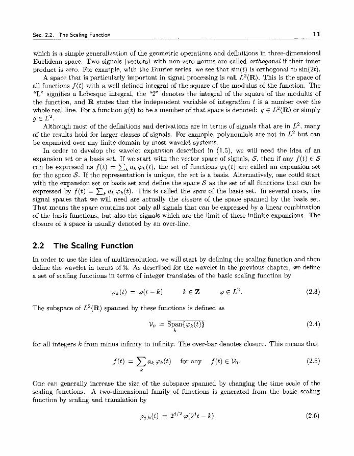
In order to agree with our intuitive ideas of scale or resolution, we formulate the basic requirement of multiresolution analysis (MRA) [Mal89c] by requiring a nesting of the spanned spaces as

(2.9)

or

(2.10)

with

V_oo = {0}, (2.11)

The space that contains high resolution signals will contain those of lower resolution also. Because of the definition of V1, the spaces have to satisfy a natural scaling condition

J(t) E v1 f(2t) E VJ+l (2.12)

which insures elements in a space are simply scaled versions of the elements in the next space. The relationship of the spanned spaces is illustrated in Figure 2.1.

The nesting of the spans of cp(21t- k), denoted by V1 and shown in (2.9) and (2.12) and graphically illustrated in Figure 2.1, is achieved by requiring that cp( t) E V1, which means that if cp(t) is in V0 , it is also in V1 , the space spanned by cp(2t). This means cp(t) can be expressed in terms of a weighted sum of shifted cp(2t) as

I cp(t) = ~ h(n) v'2 cp(2t- n), nEZ (2.13)

Sec. 2.2. The Scaling Function 13

V3 ::J v2 ::J VI ::J Vo ... ·· .··

.··: .... ·····•·····•····

Figure 2.1. Nested Vector Spaces Spanned by the Scaling Functions

where the coefficients h(n) are a sequence of real or perhaps complex numbers called the scaling function coefficients (or the scaling filter or the scaling vector) and the J2 maintains the norm of the scaling function with the scale of two.

This recursive equation is fundamental to the theory of the scaling functions and is, in some ways, analogous to a differential equation with coefficients h(n) and solution tp(t) that may or may not exist or be unique. The equation is referred to by different names to describe different interpretations or points of view. It is called the refinement equation, the multiresolution analysis (MRA) equation, or the dilation equation.

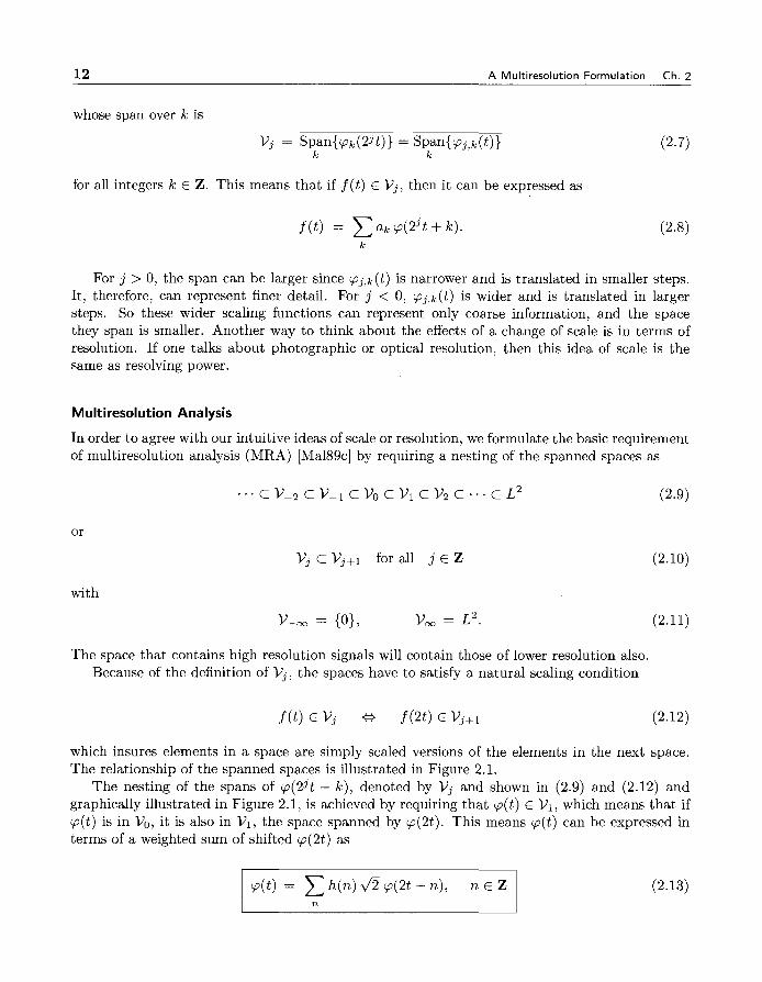
The Haar scaling function is the simple unit-width, unit-height pulse function tp(t) shown in Figure 2.2, and it is obvious that tp(2t) can be used to construct tp(t) by

tp(t) = tp(2t) + tp(2t- 1) (2.14)

which means (2.13) is satisfied for coefficients h(O) = 1/J2, h(1) = 1/J2. The triangle scaling function (also a first order spline) in Figure 2.2 satisfies (2.13) for h(O) =

2~, h(1) = ~' h(2) = .;2~' and the Daubechies scaling function shown in the first part of

--+-'dill Til...___ ¢(t) = ¢(2t) + ¢(2t- 1) cj>(t) = ~4>(2t) + 4>(2t- 1) + ~4>(2t- 2)

(a) Haar (same as 'f'D2) (b) Triangle (same as 'PSI)

Figure 2.2. Haar and Triangle Scaling Functions

14 A Multiresolution Formulation Ch. 2

Figure 6.1 satisfies (2.13) for h = {0.483, 0.8365, 0.2241, -0.1294} as do all scaling functions for their corresponding scaling coefficients. Indeed, the design of wavelet systems is the choosing of the coefficients h( n) and that is developed later.

2.3 The Wavelet Functions

The important features of a signal can better be described or parameterized, not by using IPJ,k(t) and increasing j to increase the size of the subspace spanned by the scaling functions, but by defining a slightly different set of functions 'ifJJ,k(t) that span the differences between the spaces spanned by the various scales of the scaling function. These functions are the wavelets discussed in the introduction of this book.

There are several advantages to requiring that the scaling functions and wavelets be orthog­onal. Orthogonal basis functions allow simple calculation of expansion coefficients and have a Parseval's theorem that allows a partitioning of the signal energy in the wavelet transform do­main. The orthogonal complement of V1 in VJ+ 1 is defined as W1. This means that all members of V1 are orthogonal to all members of W1. We require

(<pj,k(t), '1/Jj,R(t)) = J i.pj,k(t) '1/Jj,R(t) dt 0 (2.15)

for all appropriate j, k, C E Z. The relationship of the various subspaces can be seen from the following expressions. From

(2.9) we see that we may start at any V1, say at j = 0, and write

Vo c V1 c V2 c · · · c L 2• (2.16)

We now define the wavelet spanned subspace Wo such that

(2.17)

which extends to

(2.18)

In general this gives

(2.19)

when V0 is the initial space spanned by the scaling function <p( t- k). Figure 2.3 pictorially shows the nesting of the scaling function spaces V1 for different scales j and how the wavelet spaces are the disjoint differences (except for the zero element) or, the orthogonal complements.

The scale of the initial space is arbitrary and could be chosen at a higher resolution of, say, j = 10 to give

(2.20)

or at a lower resolution such as j = -5 to give

(2.21)

Sec. 2.3. The Wavelet Functions 15

Figure 2.3. Scaling Function and Wavelet Vector Spaces

or at even j = -oo where (2.19) becomes

(2.22)

eliminating the scaling space altogether and allowing an expansion of the form in (1.9). Another way to describe the relation of Vo to the wavelet spaces is noting

(2.23)

which again shows that the scale of the scaling space can be chosen arbitrarily. In practice, it is usually chosen to represent the coarsest detail of interest in a signal.

Since these wavelets reside in the space spanned by the next narrower scaling function, W0 C V1 , they can be represented by a weighted sum of shifted scaling function <p(2t) defined in (2.13) by

I '1/J(t) = ~ h1 (n) J2 <p(2t- n), n E Z I (2.24)

for some set of coefficients h 1(n). From the requirement that the wavelets span the "difference" or orthogonal complement spaces, and the orthogonality of integer translates of the wavelet (or scaling function), it is shown in the Appendix in (12.48) that the wavelet coefficients (modulo translations by integer multiples of two) are required by orthogonality to be related to the scaling function coefficients by

(2.25)

One example for a finite even length-N h(n) could be

(2.26)

The function generated by (2.24) gives the prototype or mother wavelet 'I(J(t) for a class of ex­pansion functions of the form

(2.27)

16 A Multiresolution Formulation Ch. 2

where 21 is the scaling oft (j is the log2 of the scale), 2-jk is the translation in t, and 21/2

maintains the (perhaps unity) L2 norm of the wavelet at different scales. The Haar and triangle wavelets that are associated with the scaling functions in Figure 2.2 are

shown in Figure 2.4. For the Haar wavelet, the coefficients in (2.24) are h1 (0) = 1/v'2, h 1 (1) = -1/ y'2 which satisfy (2.25). The Daubechies wavelets associated with the scaling functions in Figure 6.1 are shown in Figure 6.2 with corresponding coefficients given later in the book in Tables 6.1 and 6.2.

'lj;(t) = ¢(2t)- ¢(2t- 1) - 'lj;(t) = -!¢(2t)- !¢(2t- 2) + ¢(2t- 1)

(a) Haar (same as 'I/Jv2) (b) Triangle (same as '1/Jsl)

Figure 2.4. Haar and Triangle Wavelets

We have now constructed a set of functions 'Pk(t) and 'l/J1,k(t) that could span all of L 2 (R). According to (2.19), any function g(t) E L 2 (R) could be written

00 00 00

g(t) = 2:: c(k) 'Pk(t) + 2:: 2:: d(j, k) '1/Jj,k(t) (2.28) k=-oo j=O k=-oo

as a series expansion in terms of the scaling function and wavelets. In this expansion, the first summation in (2.28) gives a function that is a low resolution or

coarse approximation of g(t). For each increasing index j in the second summation, a higher or finer resolution function is added, which adds increasing detail. This is somewhat analogous to a Fourier series where the higher frequency terms contain the detail of the signal.

Later in this book, we will develop the property of having these expansion functions form an orthonormal basis or a tight frame, which allows the coefficients to be calculated by inner products as

and

c(k) = co(k) = (g(t), 'Pk(t)) = j g(t) 'Pk(t) dt

dj(k) = d(j, k) = (g(t), '1/Jj,k(t)) = J g(t) '1/Jj,k(t) dt.

(2.29)

(2.30)

The coefficient d(j, k) is sometimes written as d1(k) to emphasize the difference between the time translation index k and the scale parameter j. The coefficient c( k) is also sometimes written as c1(k) or c(j, k) if a more general "starting scale" other than j = 0 for the lower limit on the sum in (2.28) is used.