Embed Size (px)
Citation preview
HYPERBOLIC BILLIARDS AND STATISTICAL
PHYSICS
N. CHERNOV AND D. DOLGOPYAT
Abstract. Mathematical theory of billiards is a fascinating sub-ject providing a fertile source of new problems as well as conjecturetesting in dynamics, geometry, mathematical physics and spectraltheory. This survey is devoted to planar hyperbolic billiards withemphasis on their applications in statistical physics, where theyprovide many physically interesting and mathematically tractablemodels.
1. Introduction
Let D be a bounded domain on a plane or a 2D torus with piecewisesmooth boundary. A billiard system in D is generated by a single par-ticle moving freely inside D with specular reflections off the boundary∂D. The phase space of a billiard is a 3D manifold Ω; the correspondingflow Φt : Ω → Ω preserves the Liouville measure µ (which is uniform onΩ). The space of all collision points makes a 2D cross-section M ⊂ Ω,and the corresponding return map F : M → M (called billiard map)preserves a natural smooth probability measure m.
The billiard is hyperbolic if the flow Φt and the map F have non-zero Lyapunov exponents. The first class of hyperbolic billiards wasintroduced [86] by Sinai in 1970; he proved that if the boundary of D isconvex inward, then the billiard is hyperbolic, ergodic, mixing and K-mixing. He called such models dispersing billiards, now they are calledSinai billiards. They are also proven to be Bernoulli [43]. A few yearslater Bunimovich discovered [9, 10] that billiards in some domains D
2000 Mathematics Subject Classification. Primary 37D50, Secondary 34C29,60F.
Key words and phrases. Hyperbolic billiards, mixing, limit theorems.We thank our advisor Ya. G. Sinai for introducing us to this subject and constant
encouragement during our work. We thank our numerous collaborators, especiallyP. Balint, L. A. Bunimovich, R. de la Llave, G. Eyink, J. Jebowitz, R. Markarian,D. Szasz, T. Varju, L.-S. Young, and H.-K. Zhang, for many useful discussions onthe subject of this survey. NC was partially supported by NSF. DD was partiallysupported by NSF and IPST.
1
2 N. CHERNOV AND D. DOLGOPYAT
whose boundary is convex outward are also hyperbolic, due to a special‘defocusing mechanism’; the most celebrated example of his billiardsis a stadium. More general classes of planar hyperbolic billiards aredescribed in [95, 96, 63, 41]; we refer to [48, 26] for extensive surveyson hyperbolic billiards.
Billiards differ from classical smooth hyperbolic systems (Anosovand Axiom A flows and maps) in several respects. First of all, manyhyperbolic billiards have non-uniform expansion and contraction rates(for example, if the moving particle is almost tangent to a convex out-ward arc of the boundary, then it will ‘slide’, and many reflections willoccur in rapid succession during a short interval of time; a similar phe-nomenon occurs in a cusp on the boundary). Only dispersing billiardswithout cusps have uniform expansion and contraction rates.
Second, and most importantly, the billiard dynamics have singular-ities – phase points where both map F and flow Φt become discon-tinuous and have unbounded derivatives. Singularities come from twosources:
(a) Grazing collisions. In this case nearby trajectories can land onboundary components that lie far apart.
(b) Corners. In this case two nearby trajectories can hit differentboundary pieces converging to a corner and get reflected at substan-tially different angles.
Moreover, billiards without horizon (where the length of the freepath between collisions is unbounded) have infinitely many singularitycurves in phase space.
Singularities in billiards lead to an unpleasant fragmentation of phasespace. More precisely, any curve in unstable cones gets expanded (lo-cally), but the singularities may cut its image into many pieces, someof them shorter than the original curve, which then will have to spendtime on recovering. This makes billiards similar to non-uniformly hy-perbolic systems such as quadratic maps or Henon attractors.
In [97, 98] Young has proposed two general methods for studying non-uniformly hyperbolic systems: tower method and coupling method.
The first one generalizes well-known Markov partitions ([85]). Thelatter divide phase space into rectangles (‘building blocks’) that have adirect product structure and being moved under the dynamics intersectone another in a proper (Markov) way. In the tower method only onerectangle is used and its images only need to intersect itself in theMarkov way for some (not all) iterations. The tower construction isthus more flexible than that of Markov partitions, but the symbolicdynamics it provides is just as good as the one furnished by a Markovpartition.
HYPERBOLIC BILLIARDS AND STATISTICAL PHYSICS 3
The coupling method is designed to directly control the dependencebetween the past and the future. Since points with the same past his-tory form unstable manifolds, one wants to show that the images of anytwo curves in unstable cones have asymptotically the same distribution([84]). To this end one partitions those curves into small subsets andpairs subsets of the first curve with those of the second one so that theimages of the paired (coupled) points remain close to each other at alltimes (i.e. lie on the same stable manifold).
Both methods proved to be very efficient and produced many sharpresults, as we describe below. We observe here that the tower methodallows us to use functional analytic tools, in particular the theory oftransfer operators [3, 71], which provide very precise asymptotic ex-pansions. However the transfer operator approach requires a suitablydefined space of functions (observables), which is sometimes too re-strictive and dependent on the model at hand. For this reason theresults obtained by the tower approach are often less explicit and thedependence on parameters of the model is less transparent. The cou-pling approach, being more elementary if less sophisticated, gives moreexplicit bounds and makes it easier to work with several systems at atime.
Our survey is organized as follows. Section 2 describes statisticalproperties of dispersing billiards. Section 3 is devoted to systems withslow mixing rates. Section 4 deals with billiards in the presence of ex-ternal forces and discusses transport coefficients and their dependenceon parameters. Section 5 is devoted to interacting billiard particles,and Section 6 deals with infinite volume billiards.
We will denote by N (0, σ2) a normal random variable (vector) withzero mean and variance (covariance matrix) σ2, and by ρσ2 its densityfunction.
2. Dispersing billiards
Dispersing billiards make the oldest and most extensively studied classof all chaotic billiards. They, arguably, have the strongest statisticalproperties among all billiards. We need to suppose that all corners havepositively measured angles (no cusps) to guarantee uniform expansionand contraction rates.
The main difficulty in the studies of billiards is to cope with the de-structive effect of fragmentation caused by singularities (we note thatfragmentation may badly affect even relatively simple expanding mapsso that they would fail to have good statistical properties [93]). In

4 N. CHERNOV AND D. DOLGOPYAT
billiards, to cope with pathological fragmentation one imposes the fol-lowing ‘non-degeneracy’ condition: there exist m ∈ N, δ > 0, andθ0 < 1 such that for any smooth unstable curve W of length less thanδ
(1)∑
i
λi,m ≤ θ0,
where the sum runs over all smooth components Wi,m ⊂ Fm(W ) andλi,m is the factor of contraction of Wi,m under F−m. Roughly speaking(1) says that there no too-degenerate singularities such as multiplepassages through the corners. (1) always holds if there are no corners,i.e. if ∂D is smooth, because for grazing collisions the expansion factorapproaches infinity on one side of each singularity line, but in it isunknown if the condition (1) holds in dispersing billiards with corners,nor if it is really necessary for the results presented below.
Let Bdα be the space of bounded Rd-valued functions which are uni-
formly α-Holder continuous on each component of M where the mapF is smooth. We write Bα for B1
α. Let Bdα = A ∈ Bd
α : m(A) = 0. Forany function A ∈ Bd
α we denote by σ2(A) the d × d (diffusion) matrixwith components
(2) σ2ij(A) =
∞∑
n=−∞m
(
Ai (Aj T n))
(if this series converges). Denote Sn(x) =∑n−1
k=0 A(Fkx).
Theorem 1. The following four results hold under the condition (1):(a) (Exponential mixing [97, 18, 20]) There is a constant θ < 1 suchthat for every A, B ∈ Bα there is C > 0 such that for all n ∈ Z
∣
∣m(
A (B Fn))∣
∣ ≤ Cθ|n|,
which, in particular, implies the convergence of the series (2);(b) (Functional Central Limit Theorem [11, 12, 20]) For A ∈Bd
α define a continuous function Wn(t) by letting Wn(k/n) = Sk/√
nand interpolating linearly in between. Then Wn(t) weakly converges,as n → ∞, to a Brownian motion (Wiener process) with covariancematrix σ2(A).(c) (Almost sure invariance principle [66, 20]) There exist λ > 0such that for any A ∈ Bα we can find (after possibly enlarging the phasespace) a Brownian motion (Wiener process) w(t) with variance σ2(A)such that for almost all x there is n0 such that for n ≥ n0
|Sn − w(n)| < n1
2−λ
HYPERBOLIC BILLIARDS AND STATISTICAL PHYSICS 5
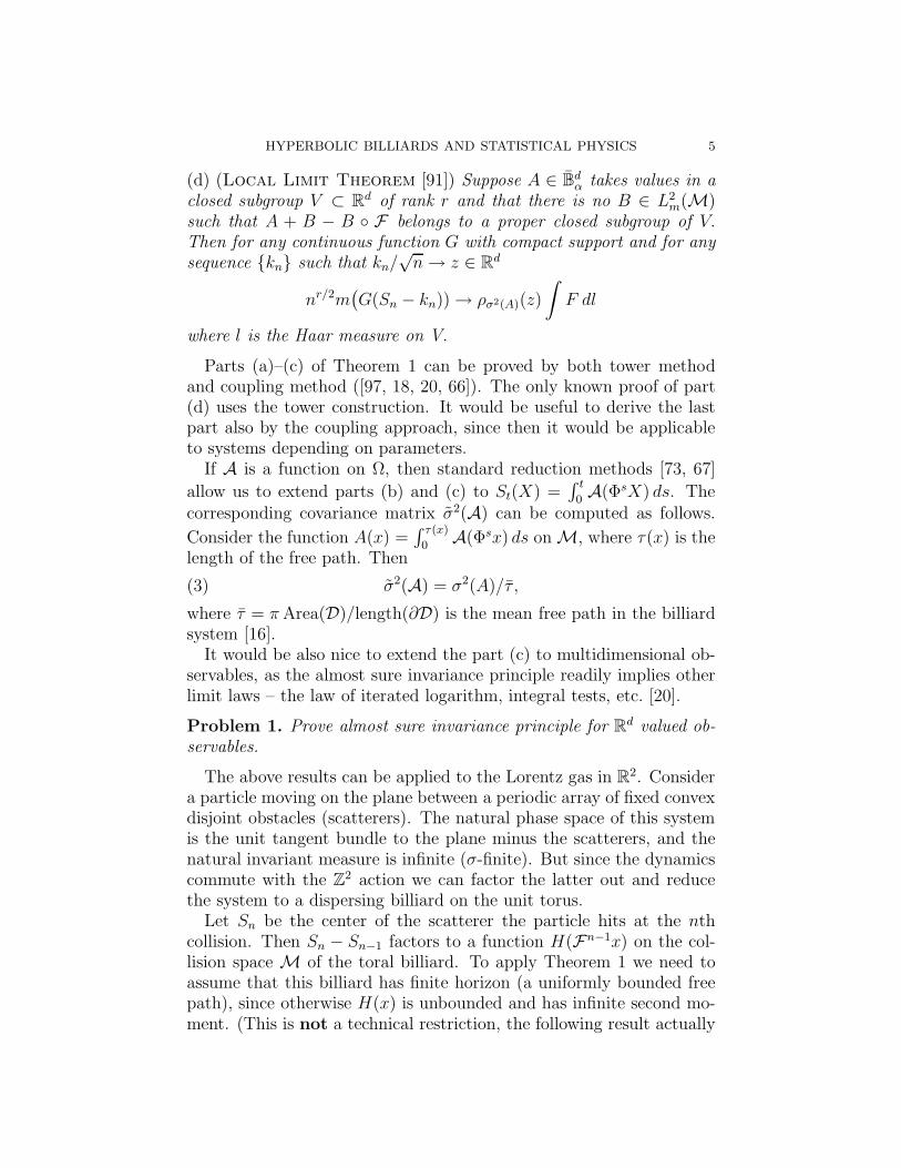
(d) (Local Limit Theorem [91]) Suppose A ∈ Bdα takes values in a
closed subgroup V ⊂ Rd of rank r and that there is no B ∈ L2m(M)
such that A + B − B F belongs to a proper closed subgroup of V.Then for any continuous function G with compact support and for anysequence kn such that kn/
√n → z ∈ Rd
nr/2m(
G(Sn − kn)) → ρσ2(A)(z)
∫
F dl
where l is the Haar measure on V.
Parts (a)–(c) of Theorem 1 can be proved by both tower methodand coupling method ([97, 18, 20, 66]). The only known proof of part(d) uses the tower construction. It would be useful to derive the lastpart also by the coupling approach, since then it would be applicableto systems depending on parameters.
If A is a function on Ω, then standard reduction methods [73, 67]
allow us to extend parts (b) and (c) to St(X) =∫ t
0A(ΦsX) ds. The
corresponding covariance matrix σ2(A) can be computed as follows.
Consider the function A(x) =∫ τ(x)
0A(Φsx) ds on M, where τ(x) is the
length of the free path. Then
(3) σ2(A) = σ2(A)/τ ,
where τ = π Area(D)/length(∂D) is the mean free path in the billiardsystem [16].
It would be also nice to extend the part (c) to multidimensional ob-servables, as the almost sure invariance principle readily implies otherlimit laws – the law of iterated logarithm, integral tests, etc. [20].
Problem 1. Prove almost sure invariance principle for Rd valued ob-
servables.
The above results can be applied to the Lorentz gas in R2. Considera particle moving on the plane between a periodic array of fixed convexdisjoint obstacles (scatterers). The natural phase space of this systemis the unit tangent bundle to the plane minus the scatterers, and thenatural invariant measure is infinite (σ-finite). But since the dynamicscommute with the Z2 action we can factor the latter out and reducethe system to a dispersing billiard on the unit torus.
Let Sn be the center of the scatterer the particle hits at the nthcollision. Then Sn − Sn−1 factors to a function H(Fn−1x) on the col-lision space M of the toral billiard. To apply Theorem 1 we need toassume that this billiard has finite horizon (a uniformly bounded freepath), since otherwise H(x) is unbounded and has infinite second mo-ment. (This is not a technical restriction, the following result actually
6 N. CHERNOV AND D. DOLGOPYAT
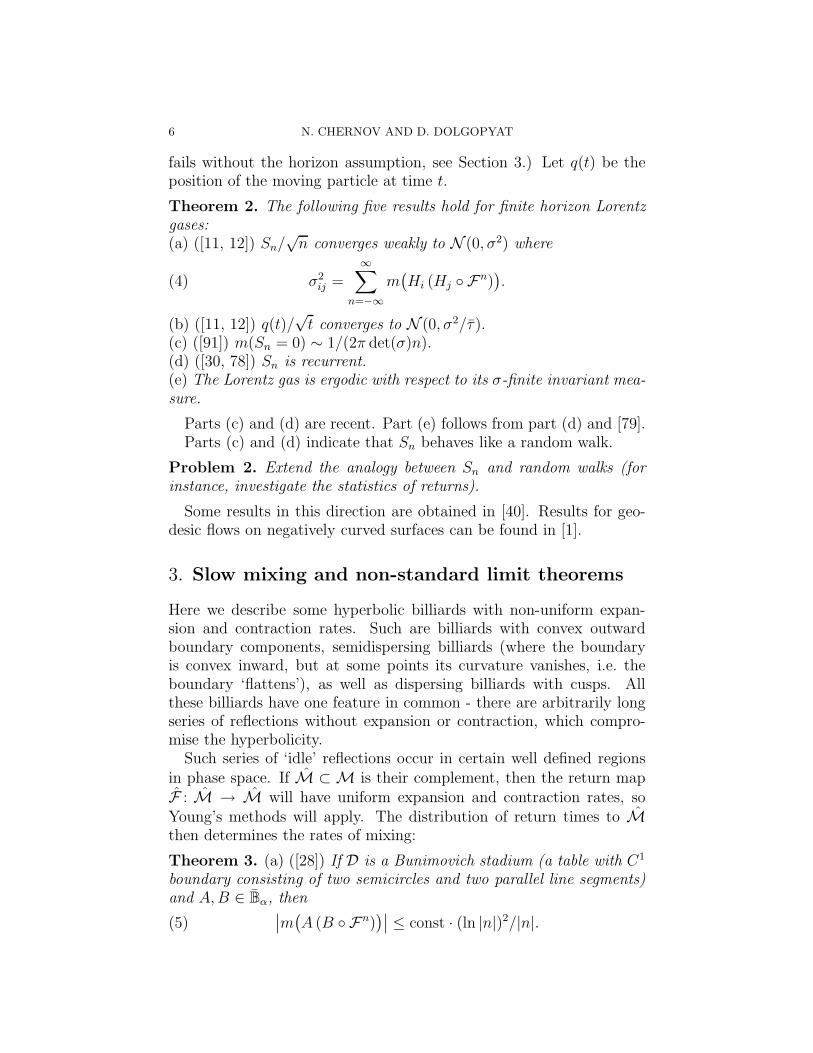
fails without the horizon assumption, see Section 3.) Let q(t) be theposition of the moving particle at time t.
Theorem 2. The following five results hold for finite horizon Lorentzgases:(a) ([11, 12]) Sn/
√n converges weakly to N (0, σ2) where
(4) σ2ij =
∞∑
n=−∞m
(
Hi (Hj Fn))
.
(b) ([11, 12]) q(t)/√
t converges to N (0, σ2/τ).(c) ([91]) m(Sn = 0) ∼ 1/(2π det(σ)n).(d) ([30, 78]) Sn is recurrent.(e) The Lorentz gas is ergodic with respect to its σ-finite invariant mea-sure.
Parts (c) and (d) are recent. Part (e) follows from part (d) and [79].Parts (c) and (d) indicate that Sn behaves like a random walk.
Problem 2. Extend the analogy between Sn and random walks (forinstance, investigate the statistics of returns).
Some results in this direction are obtained in [40]. Results for geo-desic flows on negatively curved surfaces can be found in [1].
3. Slow mixing and non-standard limit theorems
Here we describe some hyperbolic billiards with non-uniform expan-sion and contraction rates. Such are billiards with convex outwardboundary components, semidispersing billiards (where the boundaryis convex inward, but at some points its curvature vanishes, i.e. theboundary ‘flattens’), as well as dispersing billiards with cusps. Allthese billiards have one feature in common - there are arbitrarily longseries of reflections without expansion or contraction, which compro-mise the hyperbolicity.
Such series of ‘idle’ reflections occur in certain well defined regionsin phase space. If M ⊂ M is their complement, then the return mapF : M → M will have uniform expansion and contraction rates, soYoung’s methods will apply. The distribution of return times to Mthen determines the rates of mixing:
Theorem 3. (a) ([28]) If D is a Bunimovich stadium (a table with C1
boundary consisting of two semicircles and two parallel line segments)and A, B ∈ Bα, then
(5)∣
∣m(
A (B Fn))∣
∣ ≤ const · (ln |n|)2/|n|.
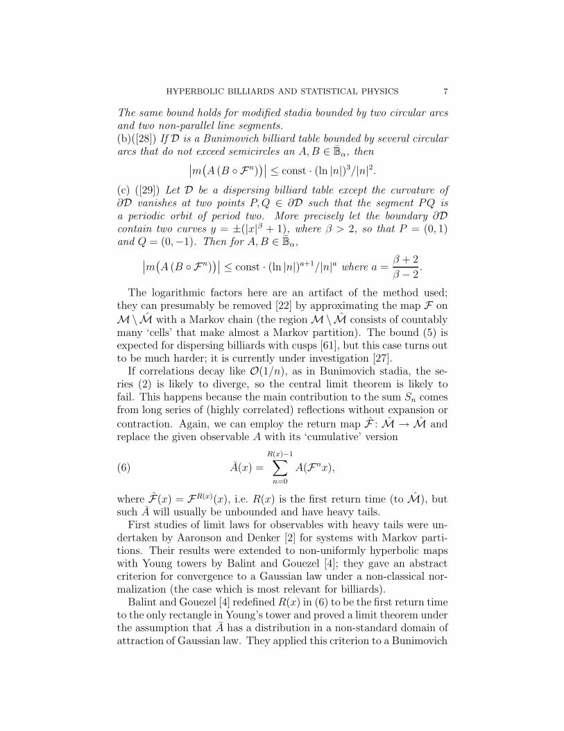
HYPERBOLIC BILLIARDS AND STATISTICAL PHYSICS 7
The same bound holds for modified stadia bounded by two circular arcsand two non-parallel line segments.(b)([28]) If D is a Bunimovich billiard table bounded by several circulararcs that do not exceed semicircles an A, B ∈ Bα, then
∣
∣m(
A (B Fn))∣
∣ ≤ const · (ln |n|)3/|n|2.(c) ([29]) Let D be a dispersing billiard table except the curvature of∂D vanishes at two points P, Q ∈ ∂D such that the segment PQ isa periodic orbit of period two. More precisely let the boundary ∂Dcontain two curves y = ±(|x|β + 1), where β > 2, so that P = (0, 1)and Q = (0,−1). Then for A, B ∈ Bα,
∣
∣m(
A (B Fn))∣
∣ ≤ const · (ln |n|)a+1/|n|a where a =β + 2
β − 2.
The logarithmic factors here are an artifact of the method used;they can presumably be removed [22] by approximating the map F on
M\M with a Markov chain (the region M\M consists of countablymany ‘cells’ that make almost a Markov partition). The bound (5) isexpected for dispersing billiards with cusps [61], but this case turns outto be much harder; it is currently under investigation [27].
If correlations decay like O(1/n), as in Bunimovich stadia, the se-ries (2) is likely to diverge, so the central limit theorem is likely tofail. This happens because the main contribution to the sum Sn comesfrom long series of (highly correlated) reflections without expansion or
contraction. Again, we can employ the return map F : M → M andreplace the given observable A with its ‘cumulative’ version
(6) A(x) =
R(x)−1∑
n=0
A(Fnx),
where F(x) = FR(x)(x), i.e. R(x) is the first return time (to M), butsuch A will usually be unbounded and have heavy tails.
First studies of limit laws for observables with heavy tails were un-dertaken by Aaronson and Denker [2] for systems with Markov parti-tions. Their results were extended to non-uniformly hyperbolic mapswith Young towers by Balint and Gouezel [4]; they gave an abstractcriterion for convergence to a Gaussian law under a non-classical nor-malization (the case which is most relevant for billiards).
Balint and Gouezel [4] redefined R(x) in (6) to be the first return timeto the only rectangle in Young’s tower and proved a limit theorem underthe assumption that A has a distribution in a non-standard domain ofattraction of Gaussian law. They applied this criterion to a Bunimovich
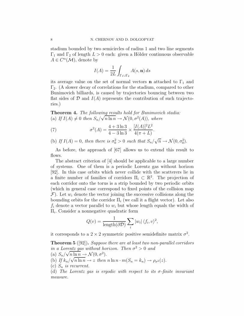
8 N. CHERNOV AND D. DOLGOPYAT
stadium bounded by two semicircles of radius 1 and two line segmentsΓ1 and Γ2 of length L > 0 each: given a Holder continuous observableA ∈ Cα(M), denote by
I(A) =1
2L
∫
Γ1∪Γ2
A(s,n) ds
its average value on the set of normal vectors n attached to Γ1 andΓ2. (A slower decay of correlations for the stadium, compared to otherBunimovich billiards, is caused by trajectories bouncing between twoflat sides of D and I(A) represents the contribution of such trajecto-ries.)
Theorem 4. The following results hold for Bunimovich stadia:(a) If I(A) 6= 0 then Sn/
√n lnn → N (0, σ2(A)), where
(7) σ2(A) =4 + 3 ln 3
4 − 3 ln 3× [I(A)]2L2
4(π + L).
(b) If I(A) = 0, then there is σ20 > 0 such that Sn/
√n → N (0, σ2
0).
As before, the approach of [67] allows us to extend this result toflows.
The abstract criterion of [4] should be applicable to a large numberof systems. One of them is a periodic Lorentz gas without horizon[92]. In this case orbits which never collide with the scatterers lie ina finite number of families of corridors Πi ⊂ R2. The projection ofeach corridor onto the torus is a strip bounded by two periodic orbits(which in general case correspond to fixed points of the collision mapF). Let wi denote the vector joining the successive collisions along thebounding orbits for the corridor Πi (we call it a flight vector). Let alsofi denote a vector parallel to wi but whose length equals the width ofΠi. Consider a nonnegative quadratic form
Q(v) =1
length(∂D)
∑
i
|wi| 〈fi, v〉2,
it corresponds to a 2 × 2 symmetric positive semidefinite matrix σ2.
Theorem 5 ([92]). Suppose there are at least two non-parallel corridorsin a Lorentz gas without horizon. Then σ2 > 0 and(a) Sn/
√n ln n → N (0, σ2).
(b) If kn/√
n ln n → z then n lnn · m(Sn = kn) → ρσ2(z).(c) Sn is recurrent.(d) The Lorentz gas is ergodic with respect to its σ-finite invariantmeasure.
HYPERBOLIC BILLIARDS AND STATISTICAL PHYSICS 9
Problem 3. Prove a functional central limit theorem in the setting of[4].
Solving this problem would lead to a complete asymptotic descriptionof the flight process in Lorentz gases without horizon.
4. Transport coefficients
Here we begin the discussion of billiard-related models of mathematicalphysics. The simplest one is a billiard D where the particle moves underan external force
(8) v = F (q, v).
Such systems were investigated in [19] under the assumptions that Dis the torus with a finite number of disjoint convex scatterers and finitehorizon. To prevent unlimited acceleration or deceleration of the par-ticle, it was assumed that there was an integral of motion (“energy”)E(q, v) such that each ray (q, αv), α ∈ R+ intersects each level surfaceE = c in exactly one point. To preserve hyperbolicity, it was assumedthat ‖F‖C1 is small.
Such forces include potential forces (F = −∇U), magnetic forces(F = B(q) × v) and electrical forces with the so called Gaussian ther-mostat:
(9) F = E(q) − 〈E(q), v〉‖v‖2
v.
Fix an energy surface E(q, v) = const containing a point with unitspeed. Under our assumptions on E this level surface is is diffeomorphicto the unit tangent bundle Ω over D and the collision space MF isdiffeomorphic to M. Denote by FF : MF → MF the correspondingreturn map.
Theorem 6 ([19]). FF has a unique SRB (Sinai-Ruelle-Bowen) mea-sure mF , i.e. for Lebesgue almost every x ∈ MF and all A ∈ C(MF )
1
n
n−1∑
i=0
A(F iFx) →
∫
MF
A dmF .
The map FF is exponentially mixing and satisfies the Central LimitTheorem (cf. Theorem 1).
As usual one can derive from this the existence (and uniqueness) ofthe SRB measure µF for the continuous time system.
Another interesting modification of billiard dynamics results fromreplacing the “hard core” collisions with the boundary by interaction
10 N. CHERNOV AND D. DOLGOPYAT
with a“soft” potential near the boundary. We do not describe suchsystems here for the lack of space referring the reader to [60].
Theorem 6 implies the existence of various transport coefficients forplanar Lorentz gas with finite horizon. For example, consider a ther-mostated electrical force (9) with a constant field E(q) = E = const,and let mE denote the SRB measure on the E = 1/2 energy surface.
Theorem 7 ([24]). There is a bilinear form ω such that for A ∈Cα(M)
mE(A) = m(A) + ω(A, E) + o(‖E‖).To illustrate these results, let qn denote the location of the particle
on the plane at its nth collision, then Theorem 6 implies for almost allx the average displacement (qn − q0)/n converges to a limit, J(E), i.e.the system exhibits an electrical current. Theorem 7 implies
J(E) = ME + o(‖E‖) (Ohm’s Law).
where M is a 2 × 2 matrix, see below.One interesting open problem is to study the dependence of the mea-
sure mF of the force F , for example the smoothness of mE as a functionof the electrical field E. For hyperbolic maps without singularities SRBmeasure depends smoothly on parameters [51, 76, 77]. For systems withsingularities the results and methods of [24] demonstrate that the SRBmeasure is differentiable at points where it has smooth densities (e.g.E = 0 in the previous example).
In fact there is an explicit expression for the derivative (Kawasakiformula). To state it let Fε be a one-parameter family of maps suchthat F0 = F has a smooth SRB measure and for small ε the map Fε
has an SRB measure mε, too, and the convergence to the steady statemε, in the sense that if ν is a smooth probability measure on M andA ∈ Cα(M) then ν(AFn
ε ) → mε(A), is exponential in n and uniformin ε. Let X = d
dε
∣
∣
ε=0(Fε F−1). Then
(10)d
dε
∣
∣
∣
ε=0mε(A) = −
∞∑
n=0
∫
Mdivm(X) A(Fnx) dm(x).
For the constant electrical field E the Kawasaki formula reads ddE
∣
∣
E=0J(E) =
12σ2, where σ2 is defined by (4). Hence
(11) J =1
2σ2E + o(‖E‖),
which is known in physics as Einstein relation.On the other hand numerical experiments [8] seem to indicate that
J(E) is not smooth for E 6= 0. Similar lack of smoothness is observed
HYPERBOLIC BILLIARDS AND STATISTICAL PHYSICS 11
in ([44, 45, 47]) for expanding interval maps, but the billiard case seemsto be more complicated. Indeed the smoothness of SRB measures (orthe lack thereof) seems to be intimately related to the dynamics of thesingularity set. For 1D maps the singularity set is finite whereas for2D maps the singularity set is one-dimensional, and so one can expectsome statistics for the evolution of that set.
Problem 4. Prove that the SRB measure, as a function of parame-ters, is not smooth (generically). Derive relations between its Holderexponent near a given parameter value and other dynamical invariants,such as Lyapunov exponents, entropy, etc.
A related issue is the dependence of infinite correlation sums, suchas the one in (10), on the geometry of the billiard table. This issuewas addressed in [23]. Given a domain D ⊂ T2, an additional roundscatterer is placed in D with a fixed radius R > 0 and a (variable)center Q; then one gets a family of billiard maps FQ acting on the samecollision space M and having a common smooth invariant measure m.For any smooth functions A, B on M let
(12) σ2A,B(Q) =
∞∑
n=−∞m
(
A (B FnQ)
)
It is proven in [23] that σ2A,B(Q) is a log-Lipschitz continuous function
of Q:(13)∣
∣σ2A,B(Q1) − σ2
A,B(Q2)∣
∣ ≤ const ∆ ln(1/∆), where ∆ = ‖Q1 − Q2‖.Problem 5. Is (13) an optimal bound?
Problem 6. Extend the analysis of [23] to dissipative systems studiedin [19].
In particular is it true that the dependence on parameters is typicallymore regular for conservative systems?
Problem 7. Consider the class S of all Sinai billiard tables on T2 anddeform a given table D continuously in C4 so that it approaches thenatural boundary of S. Investigate the limit behavior of the diffusionmatrix σ2(D).
If we only consider generic boundary points of S, then this problemsplits into three subproblems:
(a) What happens when two scatterers nearly touch each other?(b) What happens when the boundary flattens so that a periodic
trajectory with nearly zero curvature appears?
12 N. CHERNOV AND D. DOLGOPYAT
(c) What happens when one of the scatterers shrinks to a point?Analogues of Problem 7 were investigated for expanding maps [38]
and for geodesic flows on negatively curved surfaces [13]. For Sinaibilliards, only problem (c) has been tackled in [23], see Theorem 9(a)below. The first step towards problem (a) is to establish mixing boundsfor billiards with cusps (for problem (b) this task has been accomplishedin [29], see Theorem 3(c)).
One can also study the behavior of other dynamical invariants, suchas entropy and Lyapunov exponents, see [16, 32, 48, 14].
5. Interacting particles
One may hope that after so many results have been obtained for oneparticle dynamics in dispersing billiards, a comparable analysis couldbe done for multi-particle systems, including models of statistical me-chanics where the number of particles grows to infinity. However notmuch has been achieved up to now. Recently there has been a signifi-cant progress in the study of stochastically interacting particles [52, 94],but the problems involving deterministic systems appear to be muchmore difficult. One notable result is [70] where Euler equation is de-rived for Hamiltonian systems with a weak noise, however that particu-lar noise is of a very special form, and its choice remains to be justifiedby microscopic considerations.
Regarding models with finitely many particles, the most celebratedone is a gas of hard balls in a box with periodic boundary conditions(i.e. on a torus Td). The ergodicity of this system is a classical hy-pothesis in statistical mechanics attributed to L. Boltzmann and firstmathematically studied by Sinai [83, 86], see a survey [90]. The hy-perbolicity and ergodicity for this system have been proven in fairlygeneral cases only recently [80, 81], but a proof in full generality is notyet available.
Problem 8. Prove the ergodicity of N hard balls on a torus Td forevery N ≥ 3 and d ≥ 2 and for arbitrary masses m1, . . . , mN of theballs.
The existing proofs [80, 81] cover ‘generic’ mass vectors m1, . . . , mN(apart from unspecified submanifolds of codimension one in RN). Be-sides, the existing proofs heavily rely on abstract algebraic-geometricconsiderations, and it would be important to find more explicit anddynamical arguments.
A system of N hard balls on Td can be reduced to semi-dispersingbilliards in a Nd-dimensional torus with a number of multidimensional
HYPERBOLIC BILLIARDS AND STATISTICAL PHYSICS 13
cylinders removed. Now the considerations of Section 3 suggest thatthe rate of mixing for gases of hard balls is quite slow. Physicistsestimated that correlation functions for the flow decay as O(t−d/2), see[42, 72].
Problem 9. Investigate mixing rate for gases of N hard balls in Td orN hard disks on a Sinai billiard table.
An important feature of systems considered in statistical mechan-ics is that there are several different scales in space and time. Thiscan complicate the study since the problem of interest tend to involveseveral ‘levels’ of parameters, but on the other hand one can expect cer-tain simplifications; for example, Hamiltonian systems of N particleswhich are not ergodic (and this is, generically, the case due to the KAMtheory) may behave as ergodic in the thermodynamical limit N → ∞(see e.g. [31], Chapter 9). Another example is that some pathologiesslowing the mixing rates can be suppressed on large time-space scales,thus the system may behave as strongly chaotic.
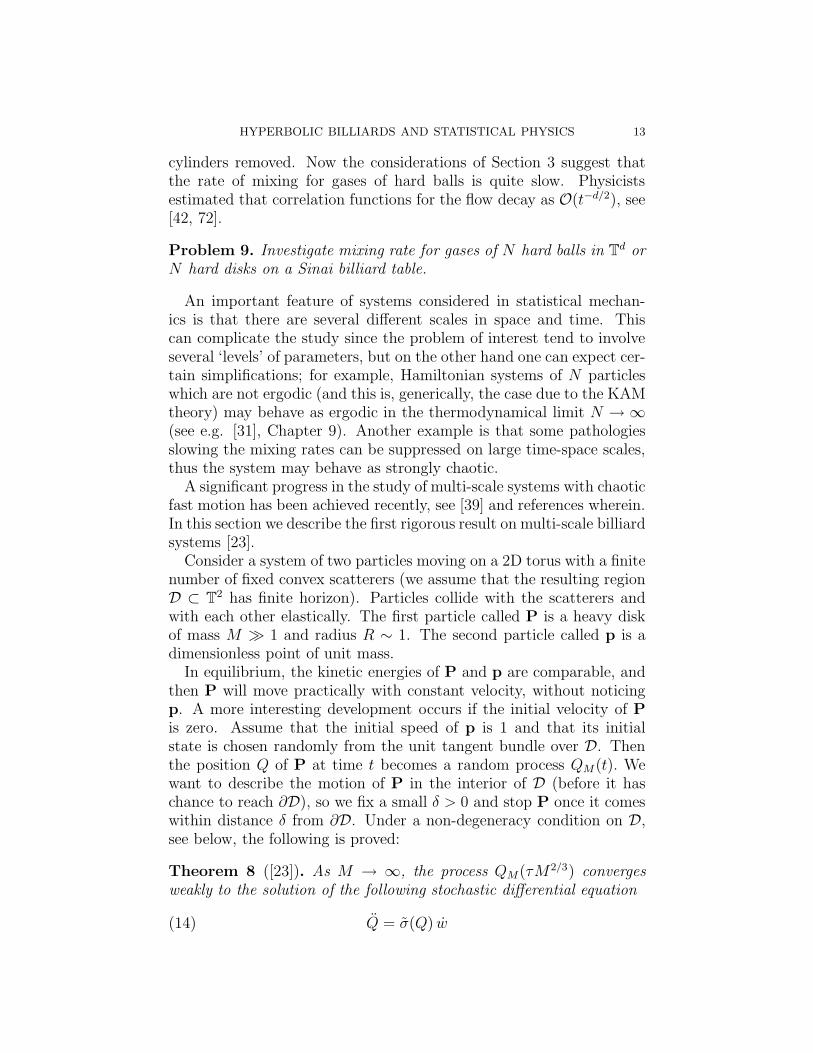
A significant progress in the study of multi-scale systems with chaoticfast motion has been achieved recently, see [39] and references wherein.In this section we describe the first rigorous result on multi-scale billiardsystems [23].
Consider a system of two particles moving on a 2D torus with a finitenumber of fixed convex scatterers (we assume that the resulting regionD ⊂ T
2 has finite horizon). Particles collide with the scatterers andwith each other elastically. The first particle called P is a heavy diskof mass M ≫ 1 and radius R ∼ 1. The second particle called p is adimensionless point of unit mass.
In equilibrium, the kinetic energies of P and p are comparable, andthen P will move practically with constant velocity, without noticingp. A more interesting development occurs if the initial velocity of P
is zero. Assume that the initial speed of p is 1 and that its initialstate is chosen randomly from the unit tangent bundle over D. Thenthe position Q of P at time t becomes a random process QM(t). Wewant to describe the motion of P in the interior of D (before it haschance to reach ∂D), so we fix a small δ > 0 and stop P once it comeswithin distance δ from ∂D. Under a non-degeneracy condition on D,see below, the following is proved:
Theorem 8 ([23]). As M → ∞, the process QM(τM2/3) convergesweakly to the solution of the following stochastic differential equation
(14) Q = σ(Q) w
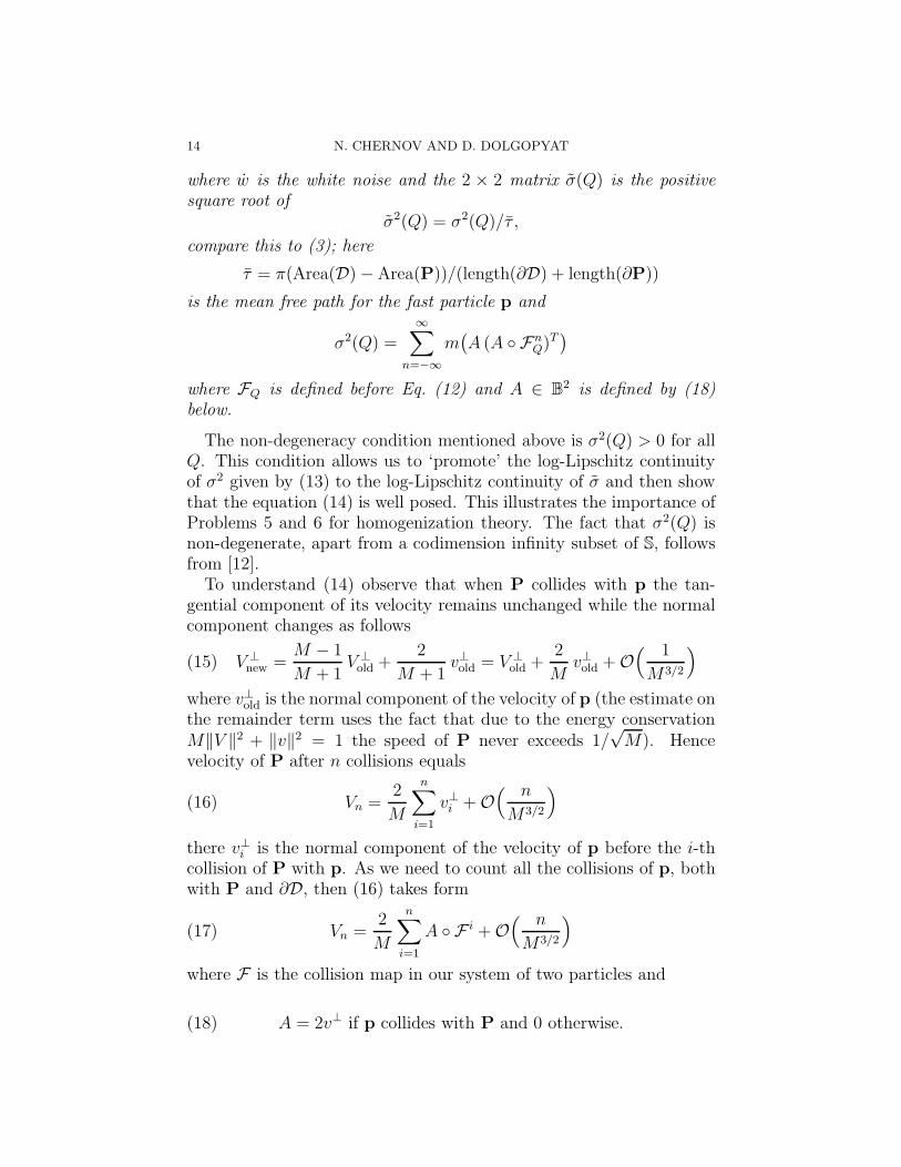
14 N. CHERNOV AND D. DOLGOPYAT
where w is the white noise and the 2 × 2 matrix σ(Q) is the positivesquare root of
σ2(Q) = σ2(Q)/τ ,
compare this to (3); here
τ = π(Area(D) − Area(P))/(length(∂D) + length(∂P))
is the mean free path for the fast particle p and
σ2(Q) =
∞∑
n=−∞m
(
A (A FnQ)T
)
where FQ is defined before Eq. (12) and A ∈ B2 is defined by (18)
below.
The non-degeneracy condition mentioned above is σ2(Q) > 0 for allQ. This condition allows us to ‘promote’ the log-Lipschitz continuityof σ2 given by (13) to the log-Lipschitz continuity of σ and then showthat the equation (14) is well posed. This illustrates the importance ofProblems 5 and 6 for homogenization theory. The fact that σ2(Q) isnon-degenerate, apart from a codimension infinity subset of S, followsfrom [12].
To understand (14) observe that when P collides with p the tan-gential component of its velocity remains unchanged while the normalcomponent changes as follows
(15) V ⊥new =
M − 1
M + 1V ⊥
old +2
M + 1v⊥old = V ⊥
old +2
Mv⊥old + O
( 1
M3/2
)
where v⊥old is the normal component of the velocity of p (the estimate on
the remainder term uses the fact that due to the energy conservationM‖V ‖2 + ‖v‖2 = 1 the speed of P never exceeds 1/
√M). Hence
velocity of P after n collisions equals
(16) Vn =2
M
n∑
i=1
v⊥i + O
( n
M3/2
)
there v⊥i is the normal component of the velocity of p before the i-th
collision of P with p. As we need to count all the collisions of p, bothwith P and ∂D, then (16) takes form
(17) Vn =2
M
n∑
i=1
A F i + O( n
M3/2
)
where F is the collision map in our system of two particles and
(18) A = 2v⊥ if p collides with P and 0 otherwise.

HYPERBOLIC BILLIARDS AND STATISTICAL PHYSICS 15
As M → ∞, our system approaches the limit where P does not move(Q ≡ const) and p bounces off ∂D∪P elastically, thus its collision mapis FQ. For this limiting system, Theorem 1(c) says that if n = Mαdτ ,then
(19)n
∑
i=1
A F iQ ∼ Mα/2 σ(Q) dw(τ)
where w(τ) is the standard Brownian motion. Since Q =∫
V dt andthe integral of the Brownian motion grows as t3/2, it is natural to takeα = 2/3 in (19), so that M3α/2/M ∼ 1, cf. (16), and expect the limitingprocess to satisfy (14).
In the proof of Theorem 8 we had to show that the two-particlecollision map F in (17) could be well approximated by the limitingbilliard map FQ in (19). While the trajectories of individual pointsunder these two maps tend to diverge exponentially fast, the images ofcurves in unstable cones tend to stay close together, and we proved thisby a probabilistic version of the shadowing lemma developed in [37].Then we decomposed the initial smooth measure into one-dimensionalmeasures on unstable curves (each curve W with a smooth measure νon it was called a standard pair) and adapted Young’s coupling methodto relate the image of each standard pair (W, ν) under the map Fn andthat under Fn
Q, as n grows.The system described above is a very simplified version of the clas-
sical Brownian motion where a macroscopic particle is submerged intoa liquid consisting of many small molecules. In our model the liquidis represented by a single particle, but its chaotic scattering off thewalls effectively replaced the chaotic motion of the molecules comingpresumably from inter-particle interactions.
One feature of Theorem 8 which may be surprising at first glanceis that the diffusion matrix σ2 is position dependent – the feature onedoes not expect for the classical Brownian particle. The reason is thatthe size of P is comparable to the size of the container D, so thattypical time between successive collisions of p with P is of order one,hence p has memory of the previous collisions with P giving rise to alocation dependent diffusion matrix. This dependence disappears if P
is macroscopically small (but microscopically large!):
Theorem 9 ([23]). As R → 0 we have
(20) σ2(Q) =8R
3Area(D)I + P(Q) R2 + o(R2),
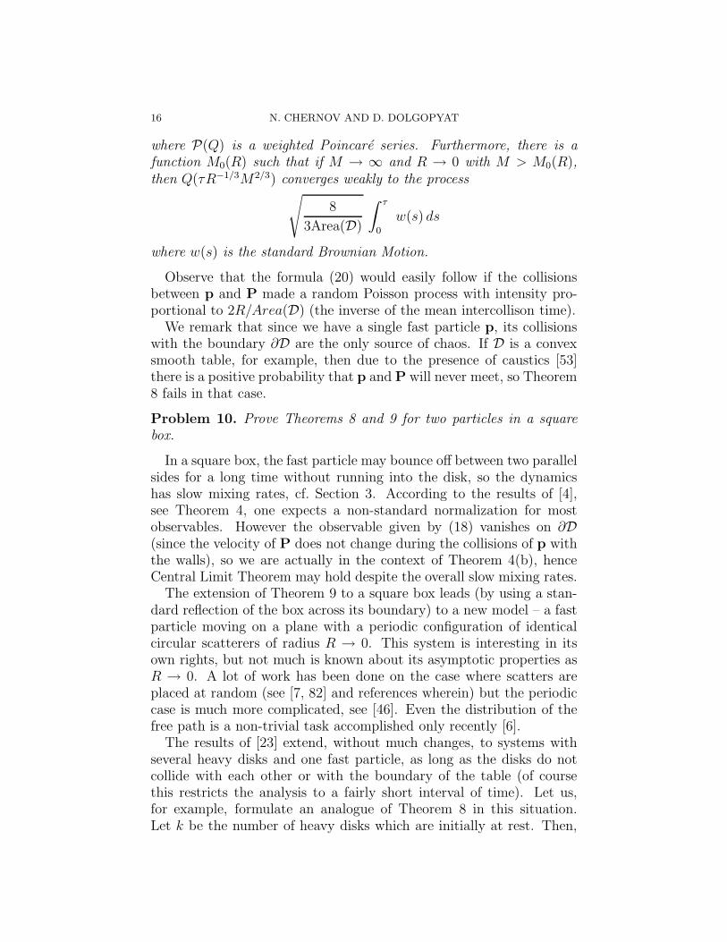
16 N. CHERNOV AND D. DOLGOPYAT
where P(Q) is a weighted Poincare series. Furthermore, there is afunction M0(R) such that if M → ∞ and R → 0 with M > M0(R),then Q(τR−1/3M2/3) converges weakly to the process
√
8
3Area(D)
∫ τ
0
w(s) ds
where w(s) is the standard Brownian Motion.
Observe that the formula (20) would easily follow if the collisionsbetween p and P made a random Poisson process with intensity pro-portional to 2R/Area(D) (the inverse of the mean intercollison time).
We remark that since we have a single fast particle p, its collisionswith the boundary ∂D are the only source of chaos. If D is a convexsmooth table, for example, then due to the presence of caustics [53]there is a positive probability that p and P will never meet, so Theorem8 fails in that case.
Problem 10. Prove Theorems 8 and 9 for two particles in a squarebox.
In a square box, the fast particle may bounce off between two parallelsides for a long time without running into the disk, so the dynamicshas slow mixing rates, cf. Section 3. According to the results of [4],see Theorem 4, one expects a non-standard normalization for mostobservables. However the observable given by (18) vanishes on ∂D(since the velocity of P does not change during the collisions of p withthe walls), so we are actually in the context of Theorem 4(b), henceCentral Limit Theorem may hold despite the overall slow mixing rates.
The extension of Theorem 9 to a square box leads (by using a stan-dard reflection of the box across its boundary) to a new model – a fastparticle moving on a plane with a periodic configuration of identicalcircular scatterers of radius R → 0. This system is interesting in itsown rights, but not much is known about its asymptotic properties asR → 0. A lot of work has been done on the case where scatters areplaced at random (see [7, 82] and references wherein) but the periodiccase is much more complicated, see [46]. Even the distribution of thefree path is a non-trivial task accomplished only recently [6].
The results of [23] extend, without much changes, to systems withseveral heavy disks and one fast particle, as long as the disks do notcollide with each other or with the boundary of the table (of coursethis restricts the analysis to a fairly short interval of time). Let us,for example, formulate an analogue of Theorem 8 in this situation.Let k be the number of heavy disks which are initially at rest. Then,
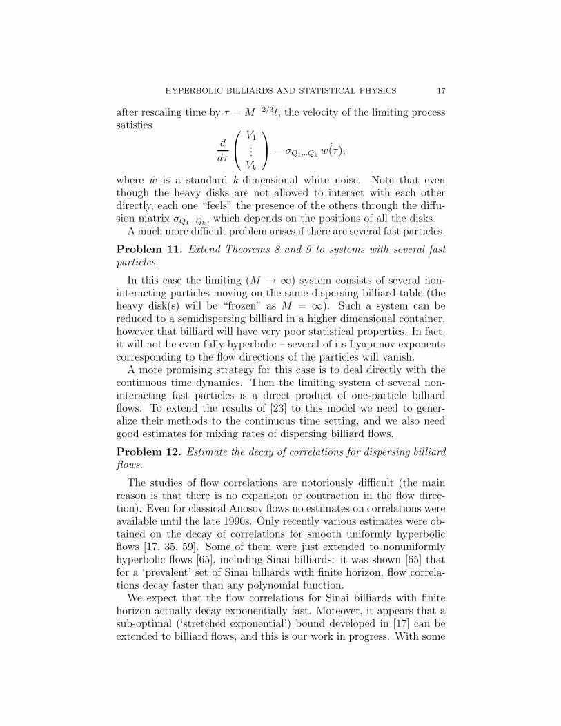
HYPERBOLIC BILLIARDS AND STATISTICAL PHYSICS 17
after rescaling time by τ = M−2/3t, the velocity of the limiting processsatisfies
d
dτ
V1...
Vk
= σQ1...Qk
˙w(τ),
where w is a standard k-dimensional white noise. Note that eventhough the heavy disks are not allowed to interact with each otherdirectly, each one “feels” the presence of the others through the diffu-sion matrix σQ1...Qk
, which depends on the positions of all the disks.A much more difficult problem arises if there are several fast particles.
Problem 11. Extend Theorems 8 and 9 to systems with several fastparticles.
In this case the limiting (M → ∞) system consists of several non-interacting particles moving on the same dispersing billiard table (theheavy disk(s) will be “frozen” as M = ∞). Such a system can bereduced to a semidispersing billiard in a higher dimensional container,however that billiard will have very poor statistical properties. In fact,it will not be even fully hyperbolic – several of its Lyapunov exponentscorresponding to the flow directions of the particles will vanish.
A more promising strategy for this case is to deal directly with thecontinuous time dynamics. Then the limiting system of several non-interacting fast particles is a direct product of one-particle billiardflows. To extend the results of [23] to this model we need to gener-alize their methods to the continuous time setting, and we also needgood estimates for mixing rates of dispersing billiard flows.
Problem 12. Estimate the decay of correlations for dispersing billiardflows.
The studies of flow correlations are notoriously difficult (the mainreason is that there is no expansion or contraction in the flow direc-tion). Even for classical Anosov flows no estimates on correlations wereavailable until the late 1990s. Only recently various estimates were ob-tained on the decay of correlations for smooth uniformly hyperbolicflows [17, 35, 59]. Some of them were just extended to nonuniformlyhyperbolic flows [65], including Sinai billiards: it was shown [65] thatfor a ‘prevalent’ set of Sinai billiards with finite horizon, flow correla-tions decay faster than any polynomial function.
We expect that the flow correlations for Sinai billiards with finitehorizon actually decay exponentially fast. Moreover, it appears that asub-optimal (‘stretched exponential’) bound developed in [17] can beextended to billiard flows, and this is our work in progress. With some
18 N. CHERNOV AND D. DOLGOPYAT
of these estimates, albeit less than optimal, we might be able to handlethe above system of several fast particles.
Interestingly, the mixing rates of the billiard flow may not matchthose of the billiard map. For instance, in Sinai billiards without hori-zon the billiard map has fast (exponential) decay of correlations [18],but the flow is apparently very slowly mixing due to long flights withoutcollisions [5]. On the contrary, in Sinai tables with cusps, the billiardmap appears to have polynomial mixing rates, see Section 3, but theflow may very well be exponentially mixing, as the particle can onlyspend a limited time in a cusp. The same happens in Bunimovichbilliards bounded only by circular arcs that do not exceed semicircles– the billiard map has slow mixing rates (Theorem 3), but the flowis possibly fast mixing, as sliding along arcs (which slows down thecollision map) does not take much flow time.
The next step toward a more realistic model of Brownian motionwould be to study several light particles of a positive radius r > 0.(If there is only one light particle, such an extension is immediatesince ‘fattening’ the light particle is equivalent to ‘fattening’ the diskP and the scatterers by the same width r.) It is however reasonable toassume that the light particles are much smaller than the heavy one,i.e. r ≪ R. In this case one can presumably treat consecutive collisionsas independent, so that in the limit r → 0 the collision process becomesMarkovian. An intermediate step in this project would be
Problem 13. Consider a system of k identical particles of radius r ≪ 1moving on a dispersing billiard table D. Let Ei(t) denote the energy ofthe ith particle at time t. Prove that the vector
E1(τ/r), E2(τ/r), . . . Ek(τ/r)
converges, as r → 0, to a Markov process with transition probabilitydensity given by the Boltzmann collision kernel [15]. This means thatif particles i and j collide so that the angles between their velocitiesand the normal are in the intervals [φi, φi + dφi] and [φj , φj + dφj],respectively, with intensity
∣
∣
√2Ei cos φi −
√
2Ej cos φj
∣
∣ dφi dφj
4π2Area(D),
and then the particle i transfers energy Ei cos2 φi − Ej cos2 φj to theparticle j.
The proof should proceed as follows. As long as the particles do notinteract, the evolution of the system is a direct product of dynamicsof individual particles. This holds true whenever the particle centers

HYPERBOLIC BILLIARDS AND STATISTICAL PHYSICS 19
q1, . . . , qk are > 2r units of length apart. Hence we need to investigatethe statistics of visits of phase orbits to
∆r = mini6=j
‖qi − qj‖ ≤ 2r,
which is a set of small measure. Visits of orbits of (weakly) hyperbolicsystems to small measure sets have been studied in many papers, see[36, 50] and the references wherein We observe that Theorem 9(a) isthe first step in the direction of Problem 13.
Next, recall that in Theorem 8 we did not allow the disk P to cometoo close to the boundary ∂D; this restricted our analysis to intervalsof time t = O(M2/3). During these times the speed of P remainssmall, ‖V ‖ = O(M−2/3), thus the system is still far from equilibrium,as M‖V ‖2 = O(M−1/3) ≪ 1.
Problem 14. Investigate the system of two particles P and p beyondthe time of the first collision of P with ∂D. In particular, how longdoes it take this system to approach equilibrium (where the energies ofthe particles become equal)?
There are two difficulties here. First, when P comes too close tothe wall ∂D, the mixing properties of the limiting (M → ∞) billiardsystem deteriorate, because a narrow channel forms between P and thewall. Once the fast particle p is trapped in that channel, it will bouncebetween P and the wall for quite a while before getting out; thus manyhighly correlated collisions between our particles occur, all pushing P inthe same direction (off the wall). Thus we expect ‖σ(Q)‖ → ∞ as thechannel narrows. The precise rate of growth of ‖σ(Q)‖ is important forthe boundary conditions for equation (14), hence Problem 7 is relevanthere.
The second difficulty is related to the accuracy of our approxima-tions. The two particle system in Theorem 8 can be put in a fairlystandard slow-fast format. Namely let (q, v) denote the position and
velocity of p and (Q, V ) those of P. Put ε = 1/√
M and denotex = (q, v/‖v‖) and y = (Q, V ) (note that ‖v‖ can be recovered from xand y due to the energy conservation). Then x and y transform at thenth collision by
xn+1 = Tyn(xn) + O(ε)
yn+1 = yn + B(xn, yn) + O(ε2)(21)
If Ty(x) is a smooth hyperbolic map, the following averaging theoremholds [39]. Let W ∋ (x0, y0) be a submanifold in the unstable cone,almost parallel to the x-coordinate space (i.e. y ≈ y0 on W ), and
20 N. CHERNOV AND D. DOLGOPYAT
such that dim W equals the dimension unstable subspace. Then for| ln ε| ≪ n ≪ 1/ε and any smooth observable A we have
(22)
∫
W
A(xn, yn) dx0 =
∫
A(x, y) dmy0(x) + ε ω(A, y0) + o(ε),
where my0 denotes the SRB measure of the map Ty0(x). This result is a
local version of Theorem 7 (consider the case yn ≡ y0!). In the presenceof singularities, however, only a weaker estimate is obtained in [23]:
(23)
∫
W
A(xn, yn) dx0 −∫
A(x, y) dmy0(x) = O(ε | ln ε|).
The extra factor | ln ε| appears because we have to wait O(| ln ε|) it-erates before the image of W under the unperturbed (billiard) mapbecomes sufficiently uniformly distributed in the collision space, andat each iteration we have to throw away a subset of measure O(ε) inthe vicinity of singularities where the shadowing is impossible. Theweak estimate (23) was sufficient for time intervals O(M2/3) consid-ered in [23] since the corresponding error term in the expression for Vn,see (17), is
O(
n
M× lnM√
M
)
= O(
ln M
M5/6
)
because n = O(M2/3). This error term is much smaller than the typicalvalue of the velocity, Vn ∼ M−2/3.
However for n ∼ M the above estimate is not good as the error termwould far exceeds the velocity itself. To improve the estimate (23) wehave to incorporate the vicinity of singularities into our analysis. Asthe singularities are one-dimensional curves, we expect points fallinginto their vicinities to have a limit distribution, as ε → 0, whose densityis smooth on each singularity curve. Finding this distribution requiresan accurate counting of billiard orbits passing near singularities. Suchcounting techniques have been applied to negatively curved manifolds[62], and we hope to extend them to billiards.
Another interesting model involving large mass ratio is so-called pis-ton problem. In that model a container is divided into two compart-ments by a heavy insulating piston, and these compartments containparticles at different temperatures. If the piston were infinitely heavy,it would not move and the temperature in each compartment wouldremain constant. However, if the mass of the piston M is finite thetemperatures would change slowly due to the energy and momenta ex-changes between the particles and the piston. There are several resultsabout infinite particle case (see [21] and references wherein) but thecase when the number of particles is finite but grows with M is much
HYPERBOLIC BILLIARDS AND STATISTICAL PHYSICS 21
more complicated (see [54]). On the other hand if the number of parti-cles is fixed and M tends to infinity then it was shown in [88, 69] underthe assumption of ergodicity of billiard in each half of the containerthat after rescaling time by 1/
√M the motion of the piston converges
to the Hamiltonian system
Q = ∆P :=K−ℓ
2πArea(D−)− K+ℓ
2πArea(D+)
where D−(D+) is the part of the container to the left(right) of thepiston K−(K+) is the energy of the particles in D−(D+) and ℓ is thelength of the piston so that ∆P is the pressure difference. In particularif ∆P = 0 and piston is initially at rest then the system does not movesignificantly during the time
√M and the question is what happens
on a longer time scale. For the infinite system it was shown in [21]that the motion converges to a diffusion process with the drift in thedirection of the hotter gas. In the finite system (for example in astadium container) this process will be accompanied by simultaneousheating of the piston so that the system may develop rapid (Q ∼ 1√
M)
oscillations. A similar phenomenon was observed numerically in [25]for a system of M2/3 particles in a 3D container. Those oscillationsmay be responsible for the fact that the system of [25] approaches itsthermal equilibrium in t ∼ Ma units of time with some 1 < a < 2(computer experiments showed that a ≈ 1.7).
In our model of two particles the formula (17) suggests that the timeof relaxation to equilibrium is of order M , as in n ∼ M collisions theheavy disk will reach its maximum velocity ‖Vn‖ ∼ √
n/M = 1/√
M ;to prove this we need to improve our approximations along the abovelines.
6. Infinite measure systems
Here we discuss several systems with infinite invariant measure, whichcan serve as tractable models of some non-equilibrium phenomena.
In ergodic theory, systems with infinite (σ-finite) invariant measureare often regarded as exotic and attract little attention. However, hy-perbolic and expanding maps with infinite invariant measure appear,more and more often, in various applications. Recently Lenci [55, 56]extended Pesin theory and Sinai’s (fundamental) ergodic theorem tounbounded dispersing billiard tables (regions under the graph of a pos-itive monotonically decreasing function y = f(x) for 0 ≤ x < ∞),
22 N. CHERNOV AND D. DOLGOPYAT
where the collision map, and often the flow as well, have infinite invari-ant measures.
Another example that we already mentioned is the periodic Lorentzgas with a diffusive particle, but this one can be reduced, because of itssymmetries, to a finite measure system by factoring out the Z2 action(Section 2). The simplest way to destroy the symmetry is to modifythe location (or shape) of finitely many scatterers in R2. We call thesefinite modifications of periodic Lorentz gases.
Theorem 10. Consider a periodic Lorentz gas with finite horizon.Then(a) ([57]) Its finite modifications are ergodic.(b) ([40]) Its finite modifications satisfy Central Limit Theorem withthe same covariance matrix as the original periodic gas does.
The proof of part (a) is surprisingly short. Every finite modificationis recurrent, because if it was not, then the particle would not comeback to the modified scatterers after some time, so it would move asif in a periodic domain, but every periodic Lorentz gas is recurrent(Theorem 2). Ergodicity then follows by [79].
The proof of (b) uses an analogy with a simple random walk (alreadyobserved in Section 2). Recall the proof of Central Limit Theorem forfinite modifications of simple random walks [89]. Let ξn be a simplerandom walk on Z2 whose transition probabilities are modified at onesite (the origin). Define ξn as follows: initially we set ξ0 = ξ0 = 0, forevery n ≥ 0 we put
ξn+1 − ξn =
ξn+1 − ξn if ξn 6= 0
Xn if ξn = 0
where Xn = ±ei, i = 1, 2, is a random unit step independent of every-thing else. Then ξn is a simple random walk and
(24) |ξn − ξn| ≤ Cardk ≤ n : ξk = 0.Since the number of visit to the origin depends only on the behaviorof the walk outside of the origin the RHS of (24) is O(ln n) (see e.g.
[33]) so Central Limit Theorem for ξn implies Central Limit Theoremfor ξn.
Let Bα denote the space of α Holder continuous functions on thecollision space of our periodic Lorentz gas with a finite modification,such that every A ∈ Bα differs from a periodic function only on acompact set and the periodic part has zero mean. Then if xn = (qn, vn)denotes the position and velocity of the particle after the nth collision
HYPERBOLIC BILLIARDS AND STATISTICAL PHYSICS 23
and x0 has a smooth distribution ν with compact support, then forA ∈ Bα∣
∣E(A(xn))∣
∣ ≤ c ν(
∃k ∈ [n−c ln n, n] : qk is on a modified scatterer)
+O(n−100),
where c > 0 is a constant. The proof of Theorem 1(d) given in [91]allows us to estimate the first term here by O(lnβ n/n) for some β > 0.The lnn factor is perhaps an artifact of the proof; on the other handeven for the much simpler case of a modified random walk one hasE(
A(ξn))
∼ c(A)/n. This implies E(
A(ξ0)A(ξn))
∼ c(A)/n. Also thereis a quadratic form q(A) such that
(25) E(
A(ξm)A(ξm+n))
∼ q(A)/n, m, n → ∞.
Here we see a new feature of non-stationary systems which does nothappen in finite ergodic theory. The correlation series
∑∞n=1 E(A(ξm)A(ξm+n))
diverges for all m but Central Limit Theorem still holds, since the con-tribution of the off-diagonal terms to E(ξ2
n) is much smaller than thecontribution of near diagonal terms.
Finite modifications of periodic Lorentz gases are among the simplestbilliards with infinite invariant measures, so we hope to move furtherin their analysis:
Problem 15. Extend (25) to finite modifications of periodic Lorentzgases (with finite horizon).
The reason for this simplicity is that finite modifications are re-stricted to a ‘codimension two’ subset of R2. The particle runs intomodified scatterer very rarely, so that its limit distribution is the sameas for the unperturbed periodic gas. The situation appears to be dif-ferent for ‘codimension one’ modifications.
For example, consider a periodic Lorentz gas and make the particlemove in the N × N box bouncing off its sides and off the scatterers inthe box. Denote by qN(t) the position of the particle at time t.
Problem 16. Prove that qN(τN2)/N converges, as N → ∞, to theBrownian motion on the unit square with mirror reflections at its bound-ary.
If the box boundaries are symmetry axis of the Lorentz gas then theresult follows easily from Theorem 1(b) but the general case appearsmore difficult. In fact if the boundaries of the box are not straightlines (so called rough boundaries) then one can expect the limit to bedifferent due to trapping and it is an interesting problem to constructsuch counterexample.
As a more sophisticated example, consider a ‘one-dimensional’ Lorentzgas – a particle moving in an infinite strip I = (x, y) : 0 ≤ y ≤ 1
24 N. CHERNOV AND D. DOLGOPYAT
(with identification (x, 0) = (x, 1)) and a periodic (in x) configurationof scatterers in I. Suppose a small external force F acts by (8) in acompact domain xmin ≤ x ≤ xmax. Denote by qF (t) the position of themoving particle at time t.
Problem 17. Find the limit distribution of qF (τN)/√
N as N → ∞.
The analogy with the random walk [89] suggests that qF (τN)/√
Nshould converge to |ζ |η where ζ and η are independent, ζ is a one-dimensional normal distribution N (0, σ2) where σ2 is the same as forthe system without the field, and η takes values ±1, so that P(η = 1) ∼P(qn > 0) depends on the evolution in the region xmin ≤ x ≤ xmax.One can further conjecture a functional limit theorem, namely thatqF (τN)/
√N converges to the so-called skew Brownian motion [49].
While the problems described above could be attacked along thelines of [40], the situation becomes much more difficult if modificationsare less regular. In particular very little is known if the location of allscatterers is purely random (if there are infinitely many independentparticles in a random Lorentz gas, ergodicity was proven by Sinai [87]).
Problem 18. Do results of Theorem 10 hold for random Lorentz gas?
The key question is the recurrence of the random Lorentz gas (thisissue is irrelevant for infinite particle systems since if one particle won-ders to infinity then another one comes to replace it, cf. [31], Chapter9).
Lenci [58] uses Theorem 10 to show that recurrence holds for an‘open dense set’ of Lorentz gases, but this remains to be shown for‘almost every’ gas in any measure-theoretic sense.
Problem 17 brings us back to billiards with external forces, seeSection 4. We assumed that (8) had an integral of motion. With-out this assumption, the system would typically heat up (the parti-cle accelerates indefinitely) or cool down (the particle slows down andstalls). It is interesting to determine which scenario occurs. Denote byK(t) = ‖v(t)‖2/2 the particle’s kinetic energy at time t.
Problem 19. Consider a Sinai billiards with a velocity-independentexternal force v = F (q). Is lim inf t→∞ K(t) finite or infinite for mostinitial conditions?
The particular case of a constant force F = const is long discussedin physics literature, see [74] and the references therein, but it is yet tobe solved mathematically. This model is known in physics as Galtonboard – a titled plane with a periodic array of pins (scatterers) and aball rolling on it under a constant (gravitational) force and bouncing

HYPERBOLIC BILLIARDS AND STATISTICAL PHYSICS 25
off the pins. Due to the conservation of the total energy, the particleaccelerates as it goes down the board. Physicists are interested infinding the limit distribution of its position (in a proper time-spacescale). Heuristic arguments [68] indicate that ‖q(t) − q(0)‖ ∼ t2/3 and‖v(t)‖ ∼ t1/3.
To address this problem observe that if we have a fast particle, i.e.K(0) = 1
2ε, then by rescaling the time variable by s = t/
√ε and de-
noting the rescaled velocity by u = dx/ds we obtain a new equation ofmotion
(26)du
ds= εF (q).
This system is of type (21) with fast variables (q, u/‖u‖) and a slowvariable T = ‖u‖2/2. For random Lorentz gases heuristic arguments[74] suggests that in a new time variable τ = const · ε−2s the limitevolution of T will be given by
(27) T =1
2√
2T+ (2T )1/4w
where w is a white noise. The same conclusion is reached in [34] forthe geodesic flow on a negatively curved surface in the presence of aweak external force.
As a side remark, observe that the fast motion is obtained here byprojecting the right hand side of (26) onto the energy surface, whichgives us a thermostated force. In particular (11) plays an importantrole in the derivation of (27). This shows that the Gaussian thermostat(9), even though regarded as ‘artificial’ by some physicists, appearsnaturally in the analysis of weakly forced systems.
We return to the conjecture (27). In terms of our original variables,equation (27) says that [K(t)]3/2 is the so called Bessel square processof index 4/3, see [75, Chapter XI]. Since this process is recurrent, itis natural to further conjecture that there is a threshold K0 > 0 suchthat for almost all initial conditions lim inft→∞ K(t) ≤ K0. This con-clusion apparently contradicts a common belief that the particle on theGalton board, see above, generally goes down and accelerates. Ratherparadoxically, it will come back up (and hence slow down) infinitelymany times! It appears that rigorous mathematics may disagree herewith physical intuition, in a spectacular way.
The first step in solving this startling paradox would be to extendthe averaging theorem (22) to billiards.
26 N. CHERNOV AND D. DOLGOPYAT
References
[1] Aaronson J., Denker M., Distributional limits for hyperbolic infinite volumegeodesic flows, Proc. Steklov Inst. 216 (1997) 174–185.
[2] Aaronson J., Denker M., Local limit theorems for partial sums of stationarysequences generated by Gibbs-Markov maps, Stoch. Dyn. 1 (2001), 193–237.
[3] Baladi V., Positive transfer operators and decay of correlations, Advanced Se-ries in Nonlinear Dynamics, v. 16, World Scientific, River Edge, NJ, 2000.
[4] Balint P., Gouezel S., Limit theorems in the stadium billiard, preprint.[5] Bleher, P. M., Statistical properties of two-dimensional periodic Lorentz gas
with infinite horizon, J. Statist. Phys. 66 (1992), 315–373.[6] Boca, F., Zaharescu, A., The distribution of the free path in the periodic
two-dimensional Lorentz gas in the small-scatterer limit, manuscript.[7] Boldrighini C., Bunimovich L. A., Sinai Ya. G. On the Boltzmann equation
for the Lorentz gas, J. Stat. Phys. 32 (1983) 477–501.[8] Bonetto F., Daems D., Lebowitz J., Properties of stationary nonequilibrium
states in the thermostated periodic Lorentz gas I: the one particle system, J.Stat. Phys. 101 (2000), 35–60.
[9] Bunimovich L. A., Billiards that are close to scattering billiards, Mat. Sb. 94
(1974), 49–73.[10] Bunimovich L. A., On the ergodic properties of nowhere dispersing billiards,
Comm. Math. Phys. 65 (1979), 295–312.[11] Bunimovich L. A., Sinai, Ya. G., Statistical properties of Lorentz gas with
periodic configuration of scatterers, Comm. Math. Phys. 78 (1980/81), 479–497.
[12] Bunimovich L. A., Sinai, Ya. G., Chernov, N. I., Statistical properties of two-dimensional hyperbolic billiards, Russ. Math. Surveys 46 (1991), 47–106.
[13] Buser P. Geometry and spectra of compact Riemann surfaces, Progr. in Math.v. 106, Birkhauser, Boston, 1992.
[14] Burago D., Ferleger S., Kononenko A., Topological entropy of semi-dispersingbilliards, Erg. Th. Dyn. Sys. 18 (1998), 791–805.
[15] Cercignani C., Illner R., Pulvirenti M., The mathematical theory of dilute gases,Appl. Math. Sciences, v. 106, Springer, New York, 1994.
[16] Chernov N., Entropy, Lyapunov exponents, and mean free path for billiards,J. Statist. Phys. 88 (1997), 1–29.
[17] Chernov N., Markov approximations and decay of correlations for Anosovflows, Ann. Math. 147 (1998), 269–324.
[18] Chernov N., Decay of correlations and dispersing billiards, J. Stat. Phys. 94
(1999), 513–556.[19] Chernov N., Sinai billiards under small external forces, Ann. Henri Poincare
2 (2001), 197–236.[20] Chernov N., Advanced statistical properties of dispersing billiards, preprint.[21] Chernov N., On a slow drift of a massive piston in an ideal gas that remains at
mechanical equilibrium, Math. Phys. Electron. J. 10 (2004), Paper 2, 18 pp.[22] Chernov N., in preparation.[23] Chernov N., Dolgopyat D., Brownian Brownian Motion - I, preprint.
HYPERBOLIC BILLIARDS AND STATISTICAL PHYSICS 27
[24] Chernov, N., Eyink, G. L., Lebowitz, J. L., Sinai Ya. G., Steady-state electricalconduction in the periodic Lorentz gas, Comm. Math. Phys. 154 (1993), 569–601.
[25] Chernov N., Lebowitz J., Dynamics of a massive piston in an ideal gas: Oscilla-tory motion and approach to equilibrium, J. Stat. Phys. 109 (2002), 507–527.
[26] Chernov N., Markarian R., Introduction to the ergodic theory of chaotic bil-liards, 2d ed. IMPA Math. Publ., 24th Brazilian Math. Colloquium, Rio deJaneiro, 2003.
[27] Chernov N., Markarian R., in preparation.[28] Chernov N., Zhang H.-K., Billiards with polynomial mixing rates, Nonlinearity
18 (2005), 1527–1553.[29] Chernov N., Zhang H.-K., A family of chaotic billiards with variable mixing
rates, Stoch. Dyn. 5 (2005), 535–553.[30] Conze, J.-P., Sur un critere de recurrence en dimension 2 pour les marches
stationnaires, applications, Erg. Th. Dyn. Sys. 19 (1999), 1233–1245.[31] Cornfeld I. P., Fomin S. V., Sinai Ya. G., Ergodic theory, Grundlehren der
Mathematischen Wissenschaften 245 (1982) Springer, New York, 1982.[32] Dahlqvist, P., The Lyapunov exponents in the Sinai billiards in the small
scatterer limit, Nonlinearity 10 (1997), 159–173.[33] Darling D. A., Kac M., On occupation times for Markoff processes, Trans.
AMS 84 (1957), 444–458.[34] de la Llave R., Dolgopyat D., Stochastic acceleration, in preparation.[35] Dolgopyat D., On decay of correlations in Anosov flows, Ann. of Math. 147
(1998), 357-390.[36] Dolgopyat D., Limit theorems for partially hyperbolic systems, Trans. AMS
356 (2004), 1637–1689.[37] Dolgopyat D., On differentiability of SRB states for partially hyperbolic sys-
tems, Inv. Math. 155 (2004), 389–449.[38] Dolgopyat D., Prelude to a kiss, Modern dynamical systems (ed. M. Brin , B.
Hasselblatt and Ya. Pesin ), Cambridge Univ Press, 2004, 313-324.[39] Dolgopyat D. Averaging and invariant measures, to appear in Moscow Math.
J.[40] Dolgopyat D., Szasz D., Varju T., Central Limit Theorem for locally perturbed
Lorentz process, in preparation.[41] Donnay V. J. Using integrability to produce chaos: billiards with positive
entropy, Comm. Math. Phys. 141 (1991), 225–257.[42] Erpenbeck J. J., Wood W. W., Molecular-dynamics calculations of the velocity-
autocorrelation function. Methods, hard-disk results, Phys. Rev. A 26 (1982),1648–1675.
[43] Gallavotti G., Ornstein D. S., Billiards and Bernoulli schemes, Comm. Math.Phys. 38 (1974), 83–101.
[44] Gaspard, P., Klages, R., Chaotic and fractal properties of deterministicdiffusion-reaction processes, Chaos 8 (1998), 409–423.
[45] Gilbert, T., Ferguson, C. D., Dorfman, J. R., Field driven thermostated sys-tem: a non-linear multi baker map, Phys. Rev. E, 59 (1999), 364-371.
[46] Golse F., Wennberg, B., On the distribution of free path lengths for the periodicLorentz gas-II, Math. Model. Numer. Anal., 34 (2000) 1151–1163.
28 N. CHERNOV AND D. DOLGOPYAT
[47] Groeneveld, J., Klages, R., Negative and nonlinear response in an exactlysolved dynamical model of particle transport, J. Stat. Phys. 109 (2002), 821–861.
[48] Hard Ball Systems and the Lorentz Gas, Edited by D. Szasz. Encyclopaedia ofMathematical Sciences, v. 101 Springer, Berlin, 2000.
[49] Harrison J. M., Shepp L. A., On skew Brownian motion, Ann. Prob. 9 (1981),309–313.
[50] Haydn N., Vaienti S., The limiting distribution and error terms for returntimes of dynamical systems, Discrete Cont. Dyn. Syst. 10 (2004), 589–616.
[51] Katok A., Knieper G., Pollicott M., Weiss H., Differentiability and analyticityof topological entropy for Anosov and geodesic flows, Inv. Math. 98 (1989),581–597.
[52] Kipnis C. & Landim C., Scaling limits of interacting particle systems,Grundlehren der Mathematischen Wissenschaften v. 320 Springer, Berlin,1999.
[53] Lazutkin V. F., Existence of caustics for the billiard problem in a convexdomain, Math. USSR (Izvestya) 37 (1973), 186–216.
[54] Lebowits J., Sinai Ya., Chernov N., Dynamics of a massive piston immersedin an ideal gas, Russian Math. Surv. 57 (2002) 1045–1125.
[55] Lenci, M., Semi-dispersing billiards with an infinite cusp-1, Comm. Math.Phys. 230 (2002), 133–180.
[56] Lenci, M., Semidispersing billiards with an infinite cusp-2,Chaos 13 (2003),105–111.
[57] Lenci M., Aperiodic Lorentz gas: recurrence and ergodicity, Erg. Th. Dyn.Sys. 23 (2003), 869–883.
[58] Lenci M., Typicality of recurrence for Lorentz gases, preprint.[59] Liverani C., On contact Anosov flows, Ann. of Math. 159 (2004), 1275–1312.[60] Liverani C., Interacting particles, in [48] pp. 179–216.[61] Machta J., Power law decay of correlations in a billiard problem, J. Statist.
Phys. 32 (1983), 555–564.[62] Margulis G. A., On some aspects of the theory of Anosov systems, With a
survey by Richard Sharp: Periodic orbits of hyperbolic flows, Springer Mono-graphs in Math. Springer-Verlag, Berlin, 2004.
[63] Markarian R., Billiards with Pesin region of measure one, Comm. Math. Phys.118 (1988), 87–97.
[64] Markarian R., Billiards with polynomial decay of correlations, Erg. Th. Dyn.Sys. 24 (2004), 177–197.
[65] Melbourne I., Rapid Decay of Correlations for Nonuniformly Hyperbolic Flows,to appear in Trans. AMS
[66] Melbourne I., Nicol M., Almost sure invariance principle for nonuniformlyhyperbolic systems, Comm. Math. Phys. 260 (2005), 131-146.
[67] Melbourne I., Torok A., Statistical limit theorems for suspension flows, IsraelJ. Math. 144 (2004), 191–209.
[68] Moran, B., Hoover, W., Bestiale S. Diffusion in a periodic Lorentz gas. J. Stat.Phys. 48, (1987) 709–726.
[69] Neishtadt A. I., Sinai, Ya. G., Adiabatic piston as a dynamical system, J. Stat.Phys. 116 (2004) 815–820.
HYPERBOLIC BILLIARDS AND STATISTICAL PHYSICS 29
[70] Olla S., Varadhan S. R. S., Yau H.-T., Hydrodynamical limit for a Hamiltoniansystem with weak noise, Comm. Math. Phys. 155 (1993), 523–560.
[71] Parry W., Pollicott M., Zeta functions and the periodic orbit structure ofhyperbolic dynamics, Asterisque 187-188 (1990), 268 pp.
[72] Pomeau Y., Resibois P., Time dependent correlation function and mode-modecoupling theories, Phys. Rep. 19 (1975), 63-139.
[73] Ratner M., The central limit theorem for geodesic flows on n-dimensional man-ifolds of negative curvature, Israel J. Math. 16 (1973), 181–197.
[74] Ravishankar K., Triolo L., Diffusive limit of Lorentz model with uniform fieldfrom the Markov approximation, Markov Proc. Rel.Fields 5 (1999), 385-421.
[75] Revuz D. & Yor M. Continuous martingales and Brownian motion,Grundlehren der Mathematischen Wissenschaften v. 293 Springer, Berlin,1999.
[76] Ruelle D., Differentiation of SRB states, Comm. Math. Phys. 187 (1997), 227–241.
[77] Ruelle D., Smooth dynamics and new theoretical ideas in nonequilibrium sta-tistical mechanics, J. Stat. Phys. 95 (1999), 393–468.
[78] Schmidt K., On joint recurrence, CRAS Paris Ser. Math. 327 (1998), 837–842.[79] Simanyi N., Towards a proof of recurrence for the Lorentz process, in Dynam-
ical systems and ergodic theory (Warsaw 1986) (ed. K. Krzyzewski) BanachCenter Publ., v .23, 265–276, PWN Warsaw, 1989.
[80] Simanyi N., Proof of the ergodic hypothesis for typical hard ball systems, Ann.Henri Poincare 5 (2004), , 203–233.
[81] Simanyi N., Proof of the Boltzmann-Sinai ergodic hypothesis for typical harddisk systems, Invent. Math. 154 (2003), 123–178.
[82] Spohn H., Large scale dynamics of interacting particles, Springer, Berlin, 1991.[83] Sinai Ya. G., On the foundations of the ergodic hypothesis for a dynamical
system of statistical mechanics, Soviet Math. Dokl. 4 (1963), 1818–1822.[84] Sinai Ya. G., Classical dynamic systems with countably-multiple Lebesgue
spectrum-II, Izv. Akad. Nauk SSSR Ser. Mat. 30 (1966) 15-68.[85] Sinai Ya. G., Markov partitions and U-diffeomorphisms. Funnk. Anal. Prilozh.
2 (1968) 64–89.[86] Sinai Ya. G., Dynamical systems with elastic reflections: Ergodic properties of
dispersing billiards, Russ. Math. Surv. 25 (1970), 137–189.[87] Sinai, Ya. G., Ergodic properties of a Lorentz gas. Funkt. Anal. Prilozh. 13
(1979), 46–59.[88] Sinai Ya. G., Dynamics of a massive particle surrounded by a finite number of
light particles, Theor., Math. Phys. 121 (1999) 1351–1357.[89] Szasz D., Telcs A., Random walk in an inhomogeneous medium with local
impurities, J. Stat. Phys. 26 (1981), 527–537.[90] Szasz D., Boltzmann’s ergodic hypothesis, a conjecture for centuries? In: Hard
ball systems and the Lorentz gas, 421–448, Encyclopaedia Math. Sci., Vol. 101,Springer, Berlin, 2000.
[91] Szasz D., Varju T., Local limit theorem for the Lorentz process and its recur-rence in the plane, Erg. Th. Dyn. Sys. 24 (2004), 257–278.
[92] Szasz D., Varju T., Limit laws and recurrence for the planar Lorentz processwith infinite horizon, preprint.

30 N. CHERNOV AND D. DOLGOPYAT
[93] Tsujii M. Piecewise expanding maps on the plane with singular ergodic prop-erties, Erg. Th. Dyn. Sys. 20 (2000), 1851–1857.
[94] Varadhan S. R. S. Entropy methods in hydrodynamic scaling, in Proceedingsof ICM-94 196–208, Birkhauser, Basel, 1995.
[95] Wojtkowski M. Invariant families of cones and Lyapunov exponents, Erg. Th.Dyn. Sys. 5 (1985), 145–161.
[96] Wojtkowski M. Principles for the design of billiards with nonvanishing Lya-punov exponents, Comm. Math. Phys. 105 (1986), 391–414.
[97] Young L.–S. Statistical properties of dynamical systems with some hyperbol-icity, Ann. Math. 147 (1998), 585–650.
[98] Young L.–S. Recurrence times and rates of mixing, Israel J. Math. 110 (1999),153–188.
Nikolai Chernov, Department of Mathematics, University of Al-
abama at Birmingham,, Birmingham AL 35294 USA
E-mail address : [email protected]: http://www.math.uab.edu/chernov/
Dmitry Dolgopyat, Department of Mathematics, University of Mary-
land, College Park MD 20742 USA
E-mail address : [email protected]: http://www.math.umd.edu/~dmitry/