Computation of Travel Time Data for Access to Destinations Study

Final Report

Prepared By:

Taek Mu Kwon, Ph.D. (Principal Investigator)Scott Klar (Research Assistant)

Transportation Data Research LaboratoryNorthland Advanced Transportation Systems Research Laboratories

Department of Electrical and Computer EngineeringUniversity of Minnesota Duluth

July 2008

Published ByCenter for Transportation Studies

University of Minnesota, Twin Cities

This report represents the results of research conducted by the author and does not necessarily represent the view or policy of the Minnesota Department of Transportation and/or the Center for Transportation Studies. This report does not contain a standard or specified technique.

The author and the Minnesota Department of Transportation and/or the Center for Transportation Studies do not endorse products or manufacturers. Trade or manufacturers’ names appear herein solely because they are considered essential to this report

Acknowledgements

This research was supported by the Northland Advanced Transportation Research Laboratories (NATSRL).

Table of Contents

Executive Summary.............................................................................................................1Chapter 1: Introduction........................................................................................................1Chapter 2: Speed Computation............................................................................................3

2.1 Background................................................................................................................32.2 Speed Computation Algorithm..................................................................................42.3 Implementation..........................................................................................................5

Chapter 3: Data Imputation Methods..................................................................................73.1 Temporal Linear Regression......................................................................................73.2 Spatial Inference Imputation....................................................................................123.3 Week-to-Week Temporal Imputation......................................................................143.4 Dynamic Time Warping..........................................................................................16

Chapter 4: Implementation of Imputations........................................................................22Chapter 5: Travel Time......................................................................................................24

5.1 Travel Time Computation........................................................................................245.2 Retrieval of Travel Time.........................................................................................26

Chapter 6: Discussions and Conclusion............................................................................29References..........................................................................................................................31

ii

List of Figures

Figure 1: 1-minute speed data..............................................................................................9Figure 2: Random deletion of values...................................................................................9Figure 3: After temporal linear regression.........................................................................10Figure 4: Converted to 5-minute data................................................................................10Figure 5: Random deletion of values.................................................................................11Figure 6: After temporal linear regression.........................................................................12Figure 7: Deleted data from 6am to 9pm...........................................................................13Figure 8: Spatially imputed data........................................................................................13Figure 9: Several weeks of data.........................................................................................14Figure 10: Deleted data from 6am to 9pm.........................................................................15Figure 11: W2W temporally imputed data........................................................................15Figure 12: Comparing spatial to W2W temporal imputation............................................16Figure 13: Data showing time stretch of afternoon peak hours.........................................17Figure 14: The minimum distance between two time series.............................................18Figure 15: Search pattern through cost matrix..................................................................18Figure 16: Legal range constraint for the warp path..........................................................19Figure 17: Warping temporal data.....................................................................................19Figure 18: DDTWA testing...............................................................................................20Figure 19: Sample corridor travel time, peak value 39.5 minutes.....................................25Figure 20: Travel time data verified by observation, 6:00am to 10:00am, 14.62mi,

1/7/2004.....................................................................................................................25Figure 21: Calculated travel time scaled, 6:00am to 10:00am, 12.3mi, 1/7/2004.............26Figure 22: A sample data retrieval code............................................................................27Figure 23: A user interface for travel time retrieval..........................................................28

List of Tables

Table 1: Comparing Imputations: Spatial Vs. Temporal...................................................16Table 2: Comparing Averaging, DTW, and DDTWA Using W2W Temporal Data........21Table 3: Average Percent of Missing Data Before and After Imputation.........................23

iii

Executive Summary

The goal of this project was to generate travel time data for the Twin Cities’ freeway network for the past 14 years and then pass the data to the Access to Destinations (AD) study team. The AD study is a new integrated approach to understand how people use the transportation system, and how transportation and land uses interact [1]. There are three major research components in the AD study [1]: (1) understanding travel dimension and reliability, (2) measuring accessibility, and (3) exploring implications of alternative transportation and land use systems. Among these components, travel time data is used as a major input for measuring travel reliability and accessibility.

When only single loop data are available, travel times are computed by first estimating speeds using volume and occupancy and then by computing link travel times between stations. However, in order to accurately compute speeds from volume and occupancy data, average vehicle length information must be known. Unfortunately, single loop data does not include the average vehicle length information. Therefore, this research developed a new procedure for computing average vehicle length information. This method conceptually works as follows. It first identifies free-flow conditions and then recursively adjusts the known speed limits to a free-flow speed. Using the adjusted free-flow speed, the average vehicle length is obtained for the identified free flow condition. Speeds are then directly computed from the volume, occupancy, and the average vehicle length. The speeds between the neighboring stations are determined by dividing into three equal-distant sections. The time for the first section is calculated with the first station’s speed, the second or middle section is calculated using an average of both stations’ speeds, and the third section is calculated using the second station’s speed. The travel time for these three sections is accumulated resulting in the total link travel time between the stations.

The historic traffic data (volume and occupancy) collected by the Regional Transportation Management Center (RTMC) at the Minnesota Department of Transportation (Mn/DOT) contains many missing data points. Data collection started with a small number in 1994 and then gradually increased to over 4,500 loop detectors. For example, about 18.3% of 1994 traffic data is missing (unknown). Causes for missing data may include major construction projects, optical fiber communication cuts, maintenance, or spot failures. The missing patterns sometimes occur at random and some other times at temporally or spatially consecutive locations. For restoring the missing data, this research applied multiple levels of spatial and temporal imputations. For simplicity, all imputation procedures were applied to the computed speeds. The three basic approaches used are linear regression, spatial imputation, and week-to-week temporal imputation. The details on these methods are described in this report. After completion of all imputation procedures, the missing percent for 1994 data was reduced from 18.3% to 3.9%. Overall (for the last fourteen years), the imputation increased the average amount of valid data from 81.7% to 98.6%. In summary, the research team successfully generated high quality travel time data for the Twin Cities’ freeways for the past 14 years. The travel time data was packed as binary arrays and then compressed for ftp distribution. Examples on how to retrieve the archived travel time data were provided along with the travel time matrices to the AD study team.

Chapter 1: Introduction

There are over 4,500 inductive loop detectors on the Twin Cities’ (Minneapolis/St. Paul) freeway system. The loop detectors are located on the mainline of freeways approximately every ½ mile and on entrance and exit ramps. Loop detectors produce the volume and occupancy of the traffic at the loop locations. Volume is the number of vehicles that pass over the loop per a period. Occupancy is the percent time the vehicles are over the loop. These two types of data are sent back via fiber optic lines to the Regional Transportation Management Center (RTMC) every 30 seconds. Every day, the volume and occupancy data from each detector is compacted into a single large file and archived. The Transportation Data Research Laboratory (TDRL) at the University of Minnesota Duluth (UMD) receives these daily archived files from RTMC and posts them through an ftp site for public uses. Presently, TDRL houses the archived traffic data starting January 1, 1994, which is the year Mn/DOT began saving the loop detector data, to present. The archived data has been the resource for many types of traffic data study by TDRL and other organizations.

Access to Destinations (AD) is an interdisciplinary research and outreach effort coordinated by the Center for Transportation Studies (CTS), with support of sponsors including the Minnesota Department of Transportation (Mn/DOT), Hennepin County, the Metropolitan Council, and the McKnight Foundation. The AD study is a new integrated approach to understand how people use the transportation system, and how transportation and land uses interact [1]. There are three major research components: (1) understanding travel dimension and reliability, (2) measuring accessibility, and (3) exploring implications of alternative transportation and land use systems.

With the availability of metro freeway loop data (volume and occupancy) for last fourteen years at TDRL, the research team at TDRL took a role in generating the travel time data of the Twin Cities’ freeway network for last fourteen years. Therefore, the objective of this research was to produce the metro freeway travel time data and pass the data to the other AD study team as one of the inputs for the study. The main challenge in computing travel times was using the data that contains missing values as much as 46 percent in some years. The basic approach employed in this research was imputation based on spatial and temporal inferences. Spatial imputation refers to replacing missing values based on spatial inferences, e.g., choosing values based on trends in relation to the neighboring stations; temporal imputation refers to utilization of temporal trends that exist within traffic data, such as morning/afternoon peak hours or weekday trends. The implementation details of these imputation methods are described in this report.

This report consists of six chapters. Chapter 2 describes the speed computation algorithm and implementation used for this research. In general, speeds cannot be accurately obtained using single loop data alone [2]. Extra information, such as vehicle classification, length, or density data is needed. The basic approach applied in this research is estimation of average vehicle lengths under free-flow conditions. Free-flow speeds vary but they are more or less close to the speed limit. An adaptive approach is used to find free-flow speeds at low occupancy time slots, which gives a distribution of average vehicle lengths of the day. After computing speeds, data imputation is applied. Chapter 3 describes spatial and temporal data imputations applied to the speed data. After

imputation, the valid data increases from about 81.7% to 98.6%. Each data imputation method is described along with examples. Chapter 4 explains implementation of imputation at a point of view of the software written. Since the imputation procedure was applied in multiple steps, this chapter is provided for clarification of how the data was produced. Chapter 5 describes the algorithm used for the link travel time based on the computed speeds and known distances. The computed speeds are only available at each station, and the speeds between two stations must be somehow estimated to compute the link travel time. A stepwise linear function as a function of distance was used and described. The distance data was obtained from the GPS coordinates available from RTMC. Once the link travel times are computed, the final travel time data is packaged into binary matrices of link travel times for each time slot. This data is zip-compressed and transferred to the AD research team. Retrieval method of travel time from this packaged data is also described in Chapter 5 along with a description of a sample program. Chapter 6 includes a discussion and concludes this report.

Chapter 2: Speed Computation

2.1 Background

In the past, many different types of speed computation algorithms have been developed and proposed. One of the fundamental relations for speed in terms of volume and occupancy is given by [2],

(1)

where

= volume, number of vehicles passed through the loop during the interval i o(i) = occupancy at time interval ig(i) = inverse of average vehicle length, i.e. T = elapsed time in hour

The above formulation requires average vehicle lengths, which are not available from single loop data. Consequently, the vehicle length information must be somehow estimated or measured for speed computation. At RTMC, the average vehicle length is computed based manual observations, i.e., g(i) is obtained from the observed speed, occupancy, and volume.

In this research, since the average vehicle length or speeds of the past data cannot be observed or reproduced, a new estimation technique was devised. This method works as follows. When the occupancy for a time slot is low (below a certain threshold, e.g. 10% was used in this research), we assume that vehicles travel at a free flow speed close to the speed limit. Utilizing the speed limit, an average vehicle length is computed for that time slot. By computing the average vehicle lengths for all time slots eligible for free flow, a distribution of vehicle lengths can be obtained, which in turn is used for free-flow speed computation. Another factor determining the speed is the relationship to density. Although many variations exist [3-6], most models follow a flat region up to a certain level of density (before congestion), and then the speed is monotonically or exponentially decreased as the density increases. The algorithm adopted for this research uses an exponential decrease function.

The speed computation algorithm using single loop data is summarized in the next section. First the algorithm computes the average field length (vehicle length plus loop width) using speed limits on low occupancy conditions. Next, using the average field lengths, free-flow speeds are computed. Finally, speeds are computed using a hybrid model of linear and exponential relation to density.

2.2 Speed Computation Algorithm

Each one-minute time slot is indexed and the parameters are notated as: N i : volume count for one-minute time slot i

o i : occupancy in percent at one-minute time slot

: average field length at one-minute time slot

: average speed at one-minute time slot : average field length of the day in feet: speed limit in miles per hour: free-flow speed in miles per hour

Step 1. Set speed limit and compute the average field length of each time slot and the average field length for the whole day.

(2)

for all where .

Set if or .

Set if .

Next, compute the average field length of the day for R time slots:

where are neither -1 nor -2 (i.e., exclude from average if -1 or -2).

Step 2. Compute the free flow speed using only occupancies .

(3)

where densities are computed using:

(4)

and

The desirable range of maximum occupancy is . Presently, we are using .

Step 3. Compute the final speeds using: If which also implies , then

(5)

If , then

(6)

If , then congested and use

(7)

where

If , then no data is available, so if before 3:00am assume

; otherwise, leave the speed as -1.

2.3 Implementation

A file called ‘r_node.xml’ provided by RTMC (it can be downloaded from http://data.dot.state.mn.us/dds/ ) contains all of the information for the stations in the corridors. It has GPS coordinates, speed limits, station id numbers, and the detector IDs for each station. Another resource is a list of the detector start dates. It lists for each detector when the occupancy data and volume data started being produced. This data was produced by TDRL by going through all of the archived traffic data starting from 1994. Speed data is only produced for stations with started detectors i.e., only for the detectors that existed and actually produced the loop data.

The speed limits are retrieved from the ‘r_node.xml’ file. Speed limits go through an adjustment based on the date of the data. This adjustment is due to the increase in posted speed limits on July 1, 1997. If the detector data is before this date then the following adjustments are made: 70mph → 65mph, 65mph → 60mph, 60mph → 55mph, and 55mph → 55mph. If the detector data was produced after the mentioned date, no speed limit adjustment is made.

Before computing speeds, the thirty-second data is converted into one-minute data. Two time slots of thirty-second volume data are added to get one-minute volume data. Two time slots of thirty-second occupancy data are averaged to get one-minute occupancy data.

The first step in the speed computation algorithm (Section 2.2) is to find the average vehicle length. For each time slice, if volume data is greater than zero and if occupancy data is greater than zero and less than ten, the field length Eq. (2) is used. The average field length is an average vehicle length plus the loop length. Once the average field length is obtained, the density for the time slot is computed using Eq. (4). The density and volume determine the free flow speed for the time slot, as given in Eq. (3).

Next the speed for each time slot is computed. If occupancy is less than 10% for the non-congested case and the field length is greater than zero, then the speed is given by Eq. (5). If occupancy is between 10% and 15%, the speed is given by Eq. (6). If occupancy is greater than 15%, the speed is given by Eq. (7). If the time is before 3:00am and there is missing data, then the speed is assumed to be a free flow speed. If volume is zero and occupancy is between 0 and 100, it is assumed that no cars entered the detectors in that time slice and the speed is again assumed to be a free flow speed. It should be noted that a free-flow speed is different from a speed limit and varies depending on the density and volume, as computed by Eq. (3).

Speed is computed for each detector (i.e. each lane), and then averaged to produce the station speed. A station speed exists if all the detectors in the station have valid speed data. If one of the detectors has missing data, the average of the rest of the detectors is used as the station speed. If more than one detector has missing data, then the station speed is set to ‘-1’, which indicates a missing data slot.

Next, five-minute speeds are calculated. The speeds of five time slots are accumulated and then divided by five to get the average five-minute speed. If one or more time slots is missing then the five-minute time slot is set to ‘-1’. The five-minute speed data is then written and saved with a name of the date such as “20070123.bin”. The station list is written followed by the data in a way that could be retrieved later and easily identified. A log file is created for each day processed. It’s a text file named according to the date of the corresponding data file. It contains the detector number and station number of detectors with no data.

Chapter 3: Data Imputation Methods

Many instances exist in the data where there are missing values randomly throughout the day. There are also entire days missing for some stations. The missing data in some years are as much as 32 percent of the data. The objective of data imputation is to estimate the missing data under the constraint that minimizes the statistical variance. Since the last form of data is five-minute station speeds, imputations are only applied to five-minute speed data. This chapter describes the imputation procedures.

3.1 Temporal Linear Regression

In a linear regression model, a method of least squares is used to find the slope and intercept of the best-fit line to the given data set. The slope ( ) and the intercept () are calculated using the following equations [10]:

(8)

(9)

where the data set is given by n pairs of .

When only a few consecutive time slots of data are missing, they are imputed by linear regression using the valid time slots nearby in time. Temporal linear regression is used in two separate instances in the production of travel times. The first instance is short duration imputation after the calculation of one-minute speed data and again after calculating five-minute speed data. The second instance is after spatial and temporal imputations have completed and before converting speed data into travel time data. The two instances use the same procedures but different durations of missing speed data.

The first instance of temporal linear regression imputation is based on a duration of three time slots. When operating on one-minute data this represents three minutes; when operating on five-minute data this represents fifteen minutes. Depending on availability in the data, this uses one, two, or three valid time slots immediately before and after each missing gap. A gap is defined by several consecutive missing time slots. A linear equation is formed (best linear fit) and used to estimate the missing data values.

The following three cases are what typically occur in the data. Notation: o = valid time slot data, x = missing time slot data

Case 1: The gaps are larger than or equal to six. Valid data from only one side of the gap is used for the linear regression. It imputes three values at the beginning and end of the gap.

(…o o o x x x…), (…x x x o o o…)

Case 2: The gap size is exactly three. Valid data is taken from both sides of the gap and all three values are imputed.

(…o o o x x x o o o…)

Case 3: The gap size is from four to five. This imputation is performed as in Case 1 except the overlap section is averaged before imputing.

(o o o x x x x o o o) | - - - - - - - | | - - - - - - - | overlap

Figures 1-4 show the effect of the imputation by linear regression. Figure 1 is the one-minute speed data for a station, which had no missing data. Figure 2 shows a random deletion of 12% of the data values, simulating the randomly missing data. Figure 3 is the result after the linear regression imputation on one-minute data and is plotted with the original data. Notice that the result of linear regression imputation is very close to the original. The data is then converted into five-minute data shown in Figure 4 and temporal linear regression is performed again if necessary. The average error of the imputed data at the five-minute data level is about 0.05 mph, measured by Root Mean Square Error (RMSE).

RMSE is computed by:

(10)

where are the values after imputation and is the original value.

Figure 1: 1-minute speed data

Figure 2: Random deletion of values

Figure 3: After temporal linear regression

Figure 4: Converted to 5-minute data

The second instance of temporal linear regression imputation is based on a duration of six time slots. When operating on five-minute data this represents thirty minutes. Depending on availability in the data, this uses one to six valid time slots immediately before and after each missing gap. A best-fit linear equation is formed and used to estimate the missing data values.

The following three cases are what typically occur in the data. (Notation: o = valid time slot data, x = missing time slot data)

Case 1: The gaps are larger than or equal to twelve. Valid data from only one side of the gap is used for the linear regression. Six values are imputed at the beginning and end of the large gap.

(…o o o o o o x x x x x x…), (…x x x x x x o o o o o o…)

Case 2: A gap size is six or less. Valid data is taken from each side of the gap and all six values are imputed.

(…o o o o o o x x x x x x o o o o o o…)

Case 3: The gap size is from seven to eleven. This imputation is performed as in Case 1 except the overlap section is averaged before imputing.

(o o o o o o x x x x x x x x o o o o o o ) | - - - - - - - - - - - - - - | | - - - - - - - - - - - - - - | overlap

The result of this second instance of temporal linear regression is shown in the following figures. Figure 5 shows the random deletion of values to a station with 100% valid data. Three cases are added to this deletion. To force the implementation of Case 2 above, the time slots between 1:15 and 1:45pm (6 slots) are deleted. To implement Case 3 the slots between 4:35 and 5:30pm (10 slots) are deleted. Case 1 is implemented by deleting time slots between 9:30 and 11:15pm (21 slots).

Figure 5: Random deletion of values

Figure 6 shows the imputed data plotted along with the original data. All the time slots are linearly imputed except for some time slots in the large gap at 9:30pm. Only 6 time slots on each end of the gap are imputed. The RMSE for the imputed data is 0.30mph.

Figure 6: After temporal linear regression

3.2 Spatial Inference Imputation

Spatial inference imputation uses the data from neighboring stations to impute missing values. It is observed that data from adjacent stations is very similar and can be used to estimate missing station data. Most stations have neighboring stations within one-half of a mile. It was decided that up to four consecutive stations can be imputed spatially. This represents about a two-mile distance. The following four cases are shown. Each time slot in the data is imputed linearly between the two good time slots from the neighboring stations. (Notation: o = station with valid time slot, x = station with missing time slot)

Case 1: One station slot is missing and has valid time slots in the neighboring stations.

(…o x o…), (x o…), (…o x)

Case 2: Data is missing in two consecutive stations.

(…o x x o…), (x x o…), (…o x x)

Case 3: Data is missing in three consecutive stations.

(…o x x x o…), (x x x o…), (…o x x x)

Case 4: Data is missing in four consecutive stations

(…o x x x x o…), (x x x x o…), (…o x x x x)

Data for missing time slots is imputed linearly from the nearest stations. It will be shown later that this spatial inference imputation is more accurate than week-to-week temporal imputation. An example of spatial imputation is shown with Figures 7 and 8. In Figure 7 data was deleted from 6:00am to 9:00pm. Figure 8 shows the result of spatial imputation plotted with the original data. The RMSE of the imputed data is 0.47 mph.

Figure 7: Deleted data from 6am to 9pm

Figure 8: Spatially imputed data

3.3 Week-to-Week Temporal Imputation

Exploring data for one day of the week for several weeks displays a trend in morning and afternoon peak hours. Week-to-week (W2W) temporal imputation uses data from the same day of the week as the missing data but from different weeks. For example, if data is missing for Monday then this method obtains statistics of data from the previous and next Mondays of the same station. Figure 9 shows several weeks of data for the same day. Notice that speeds clearly follow a W2W temporal trend.

Figure 9: Several weeks of data

W2W temporal imputation is implemented by getting data from the same station and the same day of the week from up to four weeks before and after the current date. The cases used are illustrated using the following diagram. (Notation: o = week data with valid time slot, x = week data with missing data time slot)

Cases: 1 2 3 4 5 6 o o o o o week 1x x x x o x week 2o x x x x x week 3 o x x x x week 4 o x x o week 5 o o week 6

For example, case 3 is missing data for weeks 2, 3, and 4 of say Tuesday. Data is obtained from Tuesday of weeks 1 and 5. The missing values are imputed linearly with respect to the valid data of weeks 1 and 5. If there is no valid data for many consecutive weeks then the 3 weeks nearest the valid data are imputed as in cases 5 and 6.

To show an example of W2W temporal imputation the data for a station is deleted from 6:00am to 9:00pm in Figure 10. The imputed data is shown next to the original data in Figure 11. The RMSE of the imputed data is 1.20 mph. This example implements case 1 above.

Figure 10: Deleted data from 6am to 9pm

Figure 11: W2W temporally imputed data

Next, spatial and W2W temporal imputations are compared. Almost one year of data is used to determine which method has the lowest average RMSE. The lowest average RMSE is used as a measure of the better method.

The results are summarized in Table 1. Notice that spatial imputation is clearly the more accurate estimator and the preferred method. In both cases, the average speed estimation error is less than 2mph.

Table 1: Comparing Imputations: Spatial Vs. Temporal

Method Imputation Type Average RMSE for 348 days

Average Standard Deviation

Average Spatial 0.91 0.53Average Temporal 1.36 0.73

Figure 12 is from the results of the test in Table 1. It shows the daily breakdown of average RMSE for the first four months of the year. Notice that the average of spatial imputation is better a majority of the time. This experiment suggests that only after exhausting spatial imputations, W2W temporal imputation should be applied.

Figure 12: Comparing spatial to W2W temporal imputation

3.4 Dynamic Time Warping

The question arises as to how the data from W2W temporal imputation should be combined to best estimate the missing time slot. A simple average can be taken, but averaging does not always accurately preserve the time series trends when congested time periods are of different lengths. Figure 13 illustrates the possible stretching of several weeks of speed data from a single station. The afternoon peak hours are clearly observable. However, notice that the start and durations widely vary. This section explores a method called the Dynamic Time Warping (DTW) that algorithmically finds a middle ground between two time series that have characteristics described above [7-10].

Figure 13: Data showing time stretch of afternoon peak hours

In a DTW algorithm, a two-dimensional cost matrix D(i,j) with dimensions by is formed by taking the difference between the values in the two time series

and . The algorithm finds the minimum-distance warp path traces through D(1,1) to D( , ) as illustrated in Figure 14. The warp path is found using the cost for each path and the local search pattern shown in Figure 15. The path with the least accumulated cost is chosen. This pattern must satisfy the constraint where and must be monotonically increasing.

Figure 14: The minimum distance between two time series

Figure 15: Search pattern through cost matrix

Upper and lower bounds are set to mark the legal range of the warp path. In Figure 16, the area enclosed by blue (lower bound) and green lines (upper bound) indicates the constrained area. This also forces the path to converge to end points, D(1,1) and D( , ). A line is plotted with a slope of one indicating a one-to-one relationship and no warping.

Figure 16: Legal range constraint for the warp path

The effect of DTW is illustrated in Figure 17 in that it finds a middle ground between the two time series.

Figure 17: Warping temporal data

A problem is apparent in that, after the warp path is found, the indexes are used to get values from only one of the time series. Therefore, the newly generated time series values are limited to the values of one of the time series. If the two series have different amplitudes in the congested part of the series, it is not capable of finding middle-ground amplitude. To resolve this problem a Double Dynamic Time Warping Average (DDTWA) was implemented.

DDTWA performs DTW on both time series and averages the resulting warped data together. This solves the amplitude problem previously described, but the averaging creates a new problem when the troughs of the congested sections are not aligned. The result is the lowest speeds during congestion are not accurate. This can be seen in Figure 18 using simulated data created to show the effect.

Figure 18: DDTWA testing

DDTWA in practice appears to work well in many cases. It was decided to test DTW and DDTWA against the method of simply averaging two data series. Only stations with days of entirely good data are used in this test. Sections of data are deleted and replaced using both methods. The performance metric to measure how well the imputed data matches the original data is by calculating the RMSE (Eq. 10) between the original data and the imputed data.

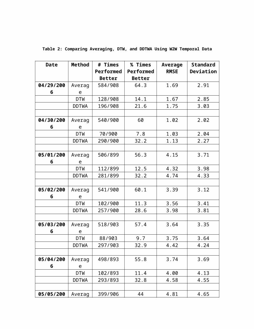
A comparison is made on all stations meeting the 100% valid data requirement. Comparing all of the stations for one week provided a good analysis as to how well each method worked. The results for Sunday April 29, 2006 through Saturday May 5, 2006 data using previous and following week data for W2W temporal imputation are summarized in Table 2.

Table 2: Comparing Averaging, DTW, and DDTWA Using W2W Temporal Data

Date Method # Times Performed

Better

% Times Performed

Better

Average RMSE

Standard Deviation

04/29/2006 Average 584/908 64.3 1.69 2.91DTW 128/908 14.1 1.67 2.85

DDTWA 196/908 21.6 1.75 3.03

04/30/2006 Average 540/900 60 1.02 2.02DTW 70/900 7.8 1.03 2.04

DDTWA 290/900 32.2 1.13 2.27

05/01/2006 Average 506/899 56.3 4.15 3.71DTW 112/899 12.5 4.32 3.98

DDTWA 281/899 32.2 4.74 4.33

05/02/2006 Average 541/900 60.1 3.39 3.12DTW 102/900 11.3 3.56 3.41

DDTWA 257/900 28.6 3.98 3.81

05/03/2006 Average 518/903 57.4 3.64 3.35DTW 88/903 9.7 3.75 3.64

DDTWA 297/903 32.9 4.42 4.24

05/04/2006 Average 498/893 55.8 3.74 3.69DTW 102/893 11.4 4.00 4.13

DDTWA 293/893 32.8 4.58 4.55

05/05/2006 Average 399/906 44 4.81 4.65DTW 158/906 17.4 4.70 4.74

DDTWA 349/906 38.6 5.30 5.43

Although DTW and DDTWA are elegant algorithms, the performance data summarized in Table 2 supports averaging. Therefore, time warping algorithms were not used for actual imputation.

Chapter 4: Implementation of Imputations

The one-minute average station speeds are calculated by averaging one-minute speeds of each lane. This is done if all the detectors in the station have valid speed data. It is also done if there are more than two stations and only one detector may have missing data. If more than one detector data is missing, then the time slot is set to ‘-1’ indicating missing data.

Short duration temporal linear regression is performed next on the one-minute data. This method imputes up to three consecutive bad values representing three minutes. The imputed values are added after the linear regression is completed so they are not used to impute other values.

One-minute data is converted into five-minute data by averaging five time slots of the one-minute data. If any time slot used in the average is missing then the five-minute time slot is set to ‘-1’ indicating missing data. This results in the percent missing data increasing slightly. This effect can be seen in Table 3 by comparing the average percent missing for one-minute and five-minute data before imputation. Short duration temporal linear regression imputation is performed again on this five-minute data.

The next imputation performs only on single missing time slots. If any single time slot is missing and it has neighboring values that are valid, then those values are averaged and inserted into the missing value. This way there are no single time slots missing going into further imputations.

Spatial imputation is performed next on the previously calculated five-minute speed data. As it was shown in Table1, spatial imputation is obviously a more accurate method, thus, it is given the priority over the W2W temporal imputation. Temporal W2W imputation follows next and uses the data resulting from the spatial imputation.

The last imputation method is larger duration linear regression. This method locates all of the gaps of missing data up to six time slots. The gaps are then imputed using linear regression. Lastly, small gaps less then one hour are located and imputed by linear regression.

The results of missing percent after imputation methods applied are summarized in Table 3. Percentage of missing data is computed before imputation and after imputation. Percent missing in five minute data is greater than that of the one minute data because of potential degradation to missing data during the five minute conversion when only one or two one minute time slots have missing data. Note that the average percent of missing values decreases to a low single digit on completion of all imputation procedures.

Table 3: Average Percent of Missing Data Before and After Imputation

Year Average % missing 30

second raw data

Average % missing before (1 min station data)

Average % missing before (5 min station data)

Average % missing after

1994 31.7 44.7 46.1 3.941995 28.3 43.6 46.7 0.561996 30.1 45.3 46.9 0.741997 25.2 37.7 39.6 1.041998 20.0 26.9 29.6 0.841999 19.2 26.1 28.9 1.402000 11.8 20.7 29.9 0.852001 12.9 22.7 34.0 1.002002 13.5 24.1 36.7 1.282003 13.6 22.9 35.3 2.562004 13.7 23.4 36.3 2.282005 11.4 21.1 35.2 0.852006 11.6 20.2 35.2 0.872007 13.2 22.0 37.5 0.89All 18.3 28.7 37.0 1.36

Chapter 5: Travel Time

5.1 Travel Time Computation

The travel time calculation uses the imputed five-minute speed data and geographical information of the stations. Mile points (MP) are calculated for every station. GPS coordinates are in meters. Eq. (11) shows the calculation of distance in miles between two GPS points and .

(11)

The first station in a corridor has a MP equal to zero miles. For each station after the first station, the distance between the current station and the previous station is calculated using the GPS coordinates of each station. This distance is added to the previous station’s MP value to get a new MP. Only stations with valid northing and easting GPS coordinates have MP values. Otherwise their MP is set to ‘-1’ and they are not used for in the calculation of travel time.

Next, a link travel time calculation is performed. The link travel time algorithm looks at two stations, their MPs, and the time slots of speed data. The distance between the two stations is divided into three equal-distant sections as shown in the following diagram. The time for the first section is calculated with the first station’s speed, the second or middle section is calculated using an average of both station’s speeds, and the third section is calculated using the second station’s speed. The time for these three sections is accumulated resulting in the total travel time between the stations.

Station 1 o---------------- ----------------- ----------------o Station2

It is monitored whether the time it takes to get to the next section is lower than the five-minute time slot. Based on the speed and distance it may occasionally take more time than one time slot to reach the next section. If this is the case, the speed from the next time slot is used in further time calculations.

An example of travel time for a selected route is shown in Figure 19. This route is U.S. 169 Southbound between stations S743 and S463. This route and day is selected because RTMC collected travel time data from human drivers for this same route and day. The accuracy of the calculated data can be obtained by comparing Figure 19 to the data in Figure 20. Figure 20 is the travel time computed by RTMC, but it is the verified data from an informal data check performed by a worker at RMTC between 6:00am and 10:00am on January 7, 2004. The person actually drove the road and recorded his travel time, which was then reported and compared with the data in Figure 20.

Figure 19: Sample corridor travel time, peak value 39.5 minutes

0:07:12

0:21:36

0:36:00

0:50:24

1:04:48

1:19:12

1:33:36

6:00:00

6:12:00

6:24:00

6:36:00

6:48:00

7:00:00

7:12:00

7:24:00

7:36:00

7:48:00

8:00:00

8:12:00

8:24:00

8:36:00

8:48:00

9:00:00

9:12:00

9:24:00

9:36:00

9:48:00

10:00:0

Figure 20: Travel time data verified by observation, 6:00am to 10:00am, 14.62mi, 1/7/2004

The graph in Figure 19 is scaled to the same time frame as the observed data in Figure 20. This results in Figure 21. The similarity between the two can be seen. The peak time of the measured data is 40.27 minutes. The peak time for the calculated data is 39.5 minutes. That is a difference of 0.77 minutes or a percent error of 1.9% for this instance. The travel times around 6:00am and 10:00am have a difference of about 4.2%. The calculated values are around 15 minutes and the observed values are around 14.4 minutes.

Figure 21: Calculated travel time scaled, 6:00am to 10:00am, 12.3mi, 1/7/2004

5.2 Retrieval of Travel Time

The travel time data that was computed and stored is the time it takes to travel between two consecutive stations at a specific time of day. These times must be retrieved and combined to give the travel time for a selected route.

Travel time is stored in two dimensional binary matrices, and a sample program written in Visual Basic (.Net) that retrieves data for one day is shown in Figure 22. First a free file is declared by putting an integer returned by the ‘FreeFile()’ function into the variable ‘fn’. The path to the data file is previously stored in the ‘filePath’ variable. Next, the travel time binary file is opened with read access using the ‘FileOpen()’ function. An integer is retrieved from the binary file using ‘FileGet()’ and is stored in the ‘sizeSI’ variable. This integer represents the size of the station index array to be retrieved. After declaring the station index array ‘SI()’ of the appropriate size, the station index array is retrieved. A two-dimensional array ‘timeData’ is declared for the travel time data using the size of the station index array and the fact that there are 288 five-minute time slots in one day. Then the travel time data is retrieved. Lastly, the binary file is closed.

Figure 22: A sample data retrieval code

The station index array is a list of station id’s e.g., ‘S870’, in which the order corresponds to the order in which the travel time data appears in the array. The index of the first dimension in the travel time array represents the specific station. The index of the second dimension contains the time data for the 288 time slots in that station. To find a station’s data, first find the station in the station index array. Record the index of its position in the array. Use this index in the travel time data array to obtain the station’s time data, i.e., timeData(station index, time slot).

Care must be taken when summing the travel times between stations. If the time sums to over five minutes, the next time slot must be used for other stations. If the time goes over ten minutes then again the next time slot must be used for further calculation. This continues until the end of the route is reached.

A sample travel time retrieval program was created with a user interface to allow the user to select origin and destination stations within a corridor. A screenshot of a user interface of a retrieval program is shown in Figure 23. The travel time binary array data can be downloaded from “ftp://tdrl.d.umn.edu/pub/ttarc/”.

Dim sizeSI As IntegerDim fn As Integer = FreeFile()FileOpen(fn, filePath, OpenMode.Binary,OpenAccess.Read)FileGet(fn, sizeSI)Dim SI(sizeSI - 1) As StringFileGet(fn, SI)Dim timeData(sizeSI - 1, 287) As SingleFileGet(fn, timeData)FileClose(fn)

Figure 23: A user interface for travel time retrieval

Chapter 6: Discussions and Conclusion

There are several other factors in addition to volume and occupancy that affect the travel time computation. A speed limit adjustment is one of them, and the adjustments were made based on the date of the speed limit change in Minnesota. If the date is before July 1, 1997 then the speed limits are lowered. The distance between two stations was obtained using the Euclidian distance of two GPS coordinates, which assumes a straight line. This may not be true for all locations. Adjustments may need to be made manually to the distances between stations on a sharply curved section of road. Another factor must be considered is the loop detector startup dates. Mn/DOT gradually increased the number of loop detectors on the freeways over the years. It started with a small number in 1994 and then gradually increased to over 4,500 loop detectors. Unfortunately, Mn/DOT did not have records on when each loop detector was activated. Therefore, the loop detector startup dates were derived from the traffic data by extracting the first time that the loop data appears on the data set.

Several data imputation methods were explored. After testing each method and comparing them based on RMSE measurements, it became clear which method was a better approximation of the missing data. This enabled us to strategically apply the imputation methods in a certain order, i.e., the best method is used first and the other less accurate methods are used after exhausting the better methods.

Linear regression imputation up to three minutes of data fills the small gaps. This method turns out to be very accurate for randomly missing data points, providing less than 0.3 mph of error.

Next, spatial imputation is applied, which turns out to be the most accurate imputation for medium to large gaps of missing data among the methods tried. The stations are usually within one-half of a mile from each other, so the effects in one station’s data quickly appear at the next station. Week-to-week (W2W) temporal imputation is applied after imputation is exhausted from the spatial imputation. This uses data from the same station and the same day of the week but from the week before and after. The trends in travel time are maintained relatively well on a week-to-week basis.

Dynamic Time Warping (DTW) was studied as a solution to how the two sets of data from spatial or temporal imputation should be combined. After implementing DTW and testing it with averaging, (see Table 2) it was apparent that averaging was more accurate in frequency in terms RMSE. Therefore, imputation computation was done using averaging rather than DTW. For the last imputation, linear regression is used to fill in the remaining gaps.

The results of these imputation methods are summarized in Table 3. Overall, it increased the average amount of valid data for all the years from 81.7% to 98.6%.

The goal of this project was to generate estimated travel times for selected routes using archived detector data for supporting the Access to Destination projects. This goal is met. A user interface now exists that allows the user to select a route and generate the travel times from 1994 to present.

For further improvements of data quality, another method may be implemented in the future to complete the imputation and have 100% valid data. This method would find

a station in which the data is the most similar to the station missing data and use its data for imputation. The most similar station would have the lowest accumulated RMSE value when comparing data two weeks previous to the date of missing data.

References [11] and [12] and the references within them are recommended for the readers who are not familiar with data imputation. In particular, [11] provides sound theoretical bases for multiple imputations, and [12] shows an application of imputation methods in short-duration and continuous count data from loop data.

References

[1] CTS, “Asking the right questions about transportation and land use,” Access to Destination Study Research Summary No. 1, Center for Transportation Studies, University of Minnesota, Minneapolis, MN, March, 2007.

[2] P. Athol, “Interdependence of certain operational characteristics within a moving traffic stream,” Highway Research Record 72, National Research Council, Washington, D.C., pp. 58-87, 1965.

[3] Denos C. Gazis, Eds, Traffic Science, John Wiley & Sons, New York, NY, 1974.

[4] R.T. Underwood, Speed, volume and density relationships: quality and theory of traffic flow, Yale University Report, New Haven, CT, 1961.

[5] D. Yao, X Gong, Y Zhang, “A hybrid model for speed estimation based on single-loop data,” IEEE Intelligent Transportation Systems Conference, Washington, DC, Oct., 2004.

[6] Y. Wang and N. Nihan, “Freeway traffic speed estimation using single loop outputs,” TRB Annual Meeting, Washington, DC, 2000.

[7] C. Myers, L. Rabiner, and A. Rosenberg, “Performance tradeoffs in dynamic time warping algorithms for isolated word recognition,” IEEE Trans. on Acoustics, Speech, and Signal Processing, Vol. ASSP-28, No. 6, pp. 623-635, Dec 1980.

[8] L. Rabiner, A. Rosenberg, and S. Levinson, “Considerations in dynamic time warping for discrete word recognition,” IEEE Trans. on Acoustics, Speech, and Signal Processing, Vol. ASSP-26, pp. 575-582, Dec 1978.

[9] Hiroaki Sakoe and Seibi Chiba, “Dynamic Programming Algorithm Optimization for Spoken Word Recognition”, IEE Trans. IEEE Trans. on Acoustics, Speech, and Signal Processing, Vol. ASSP-26, pp. 43-49, Feb 1978.

[10]W. Mendenhall, R. Scheaffer, D. Waskerly, Mathematical Statistics with Applications, 2nd Ed., Duxbury Press, Boston, MA, 1981.

[11] Little, R. J. A. and D. B. Rubin, Statistical Analysis with Missing Data, John Wiley & Sons, New York, NY, 1987.

[12] T.M. Kwon, TMC Traffic Data Automation for Mn/DOT’s Traffic Monitoring Program, Minnesota Department of Transportation, Minneapolis, MN, Report No. MN-RC-02004-29, July, 2004.