Embed Size (px)
Citation preview
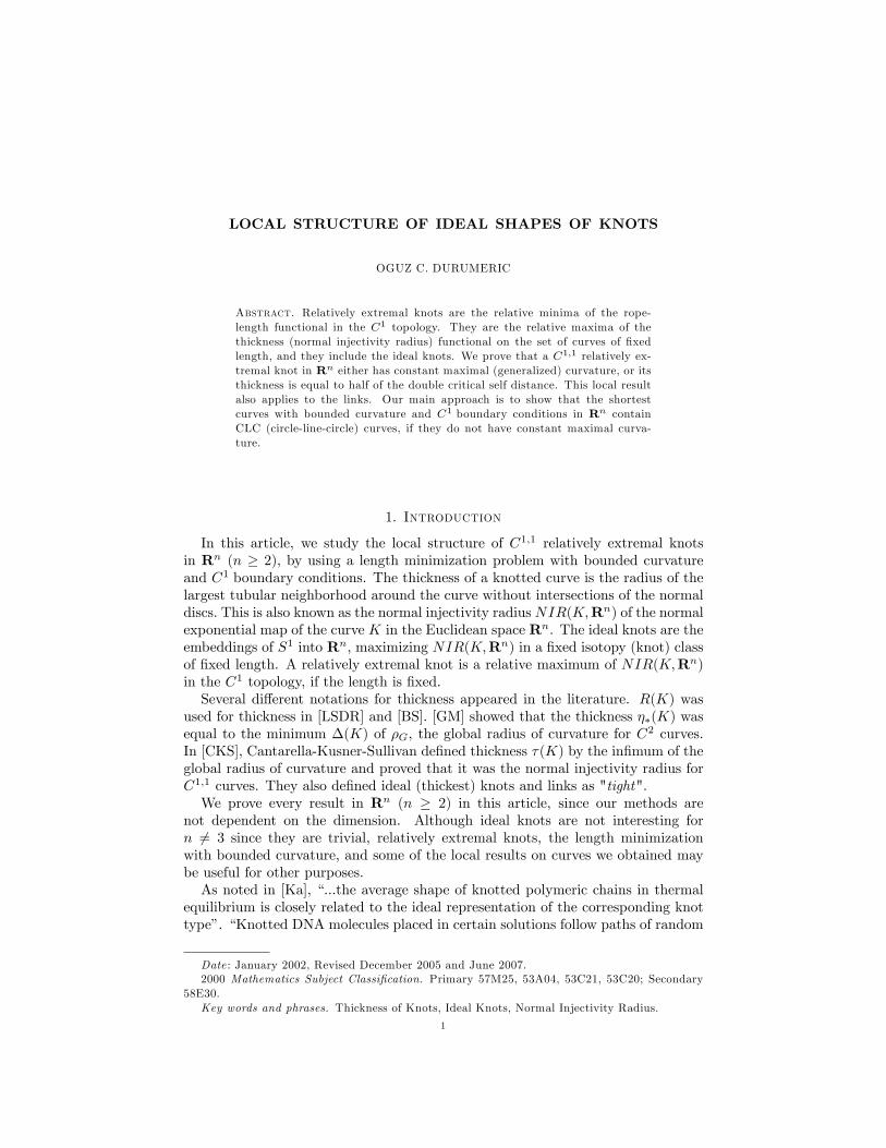
LOCAL STRUCTURE OF IDEAL SHAPES OF KNOTS
OGUZ C. DURUMERIC
Abstract. Relatively extremal knots are the relative minima of the rope-length functional in the C1 topology. They are the relative maxima of thethickness (normal injectivity radius) functional on the set of curves of �xedlength, and they include the ideal knots. We prove that a C1;1 relatively ex-tremal knot in Rn either has constant maximal (generalized) curvature, or itsthickness is equal to half of the double critical self distance. This local resultalso applies to the links. Our main approach is to show that the shortestcurves with bounded curvature and C1 boundary conditions in Rn containCLC (circle-line-circle) curves, if they do not have constant maximal curva-ture.
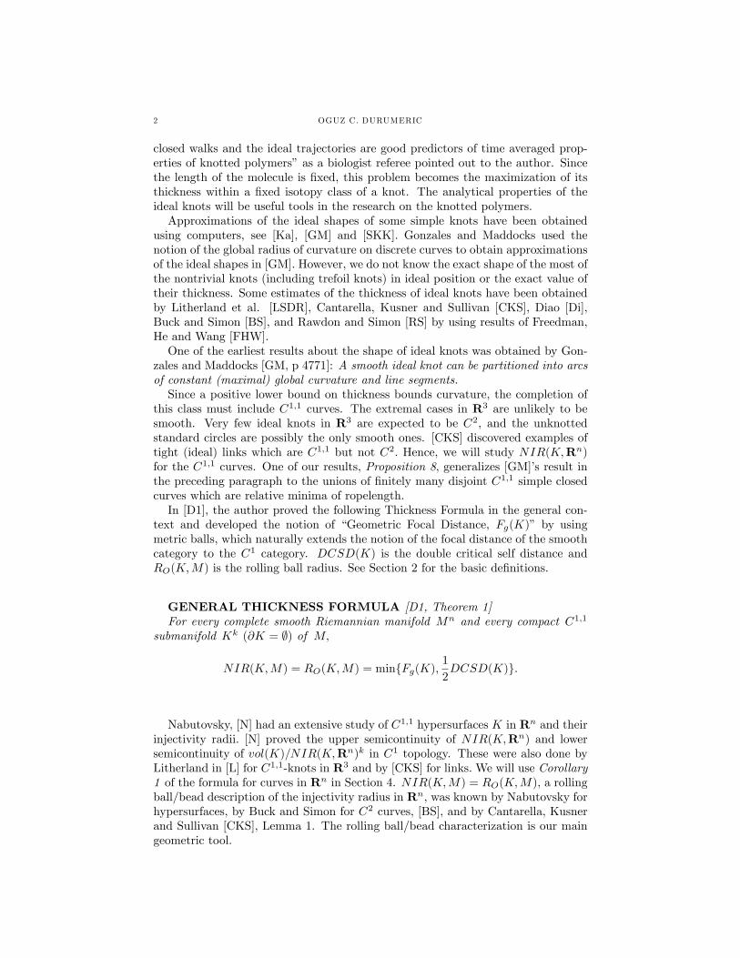
1. Introduction
In this article, we study the local structure of C1;1 relatively extremal knotsin Rn (n � 2); by using a length minimization problem with bounded curvatureand C1 boundary conditions. The thickness of a knotted curve is the radius of thelargest tubular neighborhood around the curve without intersections of the normaldiscs: This is also known as the normal injectivity radius NIR(K;Rn) of the normalexponential map of the curve K in the Euclidean space Rn. The ideal knots are theembeddings of S1 into Rn; maximizing NIR(K;Rn) in a �xed isotopy (knot) classof �xed length. A relatively extremal knot is a relative maximum of NIR(K;Rn)in the C1 topology, if the length is �xed.Several di¤erent notations for thickness appeared in the literature. R(K) was
used for thickness in [LSDR] and [BS]. [GM] showed that the thickness ��(K) wasequal to the minimum �(K) of �G, the global radius of curvature for C2 curves.In [CKS], Cantarella-Kusner-Sullivan de�ned thickness �(K) by the in�mum of theglobal radius of curvature and proved that it was the normal injectivity radius forC1;1 curves. They also de�ned ideal (thickest) knots and links as "tight".We prove every result in Rn (n � 2) in this article, since our methods are
not dependent on the dimension. Although ideal knots are not interesting forn 6= 3 since they are trivial, relatively extremal knots, the length minimizationwith bounded curvature, and some of the local results on curves we obtained maybe useful for other purposes.As noted in [Ka], �...the average shape of knotted polymeric chains in thermal
equilibrium is closely related to the ideal representation of the corresponding knottype�. �Knotted DNA molecules placed in certain solutions follow paths of random
Date : January 2002, Revised December 2005 and June 2007.2000 Mathematics Subject Classi�cation. Primary 57M25, 53A04, 53C21, 53C20; Secondary
58E30.Key words and phrases. Thickness of Knots, Ideal Knots, Normal Injectivity Radius.
1
2 OGUZ C. DURUMERIC
closed walks and the ideal trajectories are good predictors of time averaged prop-erties of knotted polymers�as a biologist referee pointed out to the author. Sincethe length of the molecule is �xed, this problem becomes the maximization of itsthickness within a �xed isotopy class of a knot. The analytical properties of theideal knots will be useful tools in the research on the knotted polymers.Approximations of the ideal shapes of some simple knots have been obtained
using computers, see [Ka], [GM] and [SKK]. Gonzales and Maddocks used thenotion of the global radius of curvature on discrete curves to obtain approximationsof the ideal shapes in [GM]. However, we do not know the exact shape of the most ofthe nontrivial knots (including trefoil knots) in ideal position or the exact value oftheir thickness. Some estimates of the thickness of ideal knots have been obtainedby Litherland et al. [LSDR], Cantarella, Kusner and Sullivan [CKS], Diao [Di],Buck and Simon [BS], and Rawdon and Simon [RS] by using results of Freedman,He and Wang [FHW].One of the earliest results about the shape of ideal knots was obtained by Gon-
zales and Maddocks [GM, p 4771]: A smooth ideal knot can be partitioned into arcsof constant (maximal) global curvature and line segments.Since a positive lower bound on thickness bounds curvature, the completion of
this class must include C1;1 curves. The extremal cases in R3 are unlikely to besmooth. Very few ideal knots in R3 are expected to be C2, and the unknottedstandard circles are possibly the only smooth ones. [CKS] discovered examples oftight (ideal) links which are C1;1 but not C2: Hence, we will study NIR(K;Rn)for the C1;1 curves. One of our results, Proposition 8, generalizes [GM]�s result inthe preceding paragraph to the unions of �nitely many disjoint C1;1 simple closedcurves which are relative minima of ropelength.In [D1], the author proved the following Thickness Formula in the general con-
text and developed the notion of �Geometric Focal Distance, Fg(K)� by usingmetric balls, which naturally extends the notion of the focal distance of the smoothcategory to the C1 category. DCSD(K) is the double critical self distance andRO(K;M) is the rolling ball radius. See Section 2 for the basic de�nitions:
GENERAL THICKNESS FORMULA [D1, Theorem 1]For every complete smooth Riemannian manifold Mn and every compact C1;1
submanifold Kk (@K = ;) of M;
NIR(K;M) = RO(K;M) = minfFg(K);1
2DCSD(K)g:
Nabutovsky, [N] had an extensive study of C1;1 hypersurfaces K in Rn and theirinjectivity radii: [N] proved the upper semicontinuity of NIR(K;Rn) and lowersemicontinuity of vol(K)=NIR(K;Rn)k in C1 topology. These were also done byLitherland in [L] for C1;1-knots in R3 and by [CKS] for links:We will use Corollary1 of the formula for curves in Rn in Section 4. NIR(K;M) = RO(K;M); a rollingball/bead description of the injectivity radius in Rn, was known by Nabutovsky forhypersurfaces, by Buck and Simon for C2 curves, [BS], and by Cantarella, Kusnerand Sullivan [CKS], Lemma 1. The rolling ball/bead characterization is our maingeometric tool.
3
For a C1;1 curve ; 00 exists almost everywhere by Rademacher�s Theorem, [F].For a C1;1 curve (s) parametrized by the arclength s, de�ne the (generalized) cur-vature � (s) = lim sup
x6=y!s
]( 0(x); 0(y))jx�yj for all s and the analytic focal distance Fk( ) =
(sup � )�1: For K with several components, take the smallest focal distance of the
components. See Lemmas 1 and 2, for a proof of Fg( ) = Fk( ) = (ess sup k 00k)�1for curves parametrized by arclength in Rn, and [D1, Proposition 12] for a similarcurvature description of Fg(Kk) for higher dimensional Kk � Rn:
Corollary 1. (Thickness Formula) For every union K of �nitely many disjointC1;1 simple closed curves in Rn, one hasNIR(K;M) = RO(K;M) = minfFk(K); 12DCSD(K)g:Thickness Formula was �rst discussed for C2�knots in R3 in [LSDR], and for
C1;1 knots in R3 by Litherland in [L], without RO. [CKS, Lemma 1] proved theThickness Formula for C1;1 knots and links in R3; since Fg = Fk:The notion of the global radius of curvature �G was developed by Gonzales
and Maddocks in [GM] for smooth curves in R3, de�ned by using circles passingthrough triple distinct points of the curve. This gives another characterization:NIR(K;R3) = infK �G, [GM]. This is still true for all C1 curves by [CKS, Lemma1]. The construction of �G and RO for curves in R3 are di¤erent in nature due to 3-point intersection condition versus 1-point of tangency and 1-point of intersectioncondition. However, at their in�ma they are the same quantity: NIR(K;R3);[CKS, Lemma 1]. Although the equality NIR(K;M) = RO(K;M) is generalizableto all dimensions and Riemannian manifolds [D1], the notion of �G may not bee¤ective beyond the spaces of constant curvature.
Remark 1. In this article, we study the pieces of relatively extremal knots awayfrom the points of minimal double critical self distance by using minimization oflength with curvature bounded by �. Since all problems we discuss are in Rn; wecan rescale and take � = 1 to simplify our statements and proofs.
Problem 1. (Markov [M]-Dubins [Du]) Given p; q; v; w inRn; with kvk = kwk = 1:Classify all shortest curves in C(p; q; v; w) which is the set of all curves betweenthe points p and q in Rn with 0(p) = v, 0(q) = w and � � 1 = �.A CLC(circle-line-circle) curve is one circular arc followed by a line segment and
then by another circular arc in a C1 fashion (like two letters J with common straightparts, one hook at each end, and possibly non-coplanar, see Figure 10 ), where thecircular arcs have radius 1:We will use CLC(�) if the upper bound of curvature is�: Similarly, one can de�ne CCC -curves by C1�concatenation of 3 arcs of circlesof the same curvature. If p = q and v = �w, then the shortest curve with curvaturerestriction satis�es � � 1 and it is not a CLC -curve, see the examples and remarksfollowing the proof of Theorem 1 as well as Figure 11. One can construct curvesof constant (generalized) curvature 1 such that the curve is not twice di¤erentiableat countably in�nite points.We note that the classi�cation of shortest curves in C(p; q; v; w) with � � 1 is not
a simple matter. Markov [M], Dubins [Du] and Reeds and Shepp [ReSh] studied the2 dimensional cases. In dimension 3, the following results of H. Sussmann obtainedthe possible types solutions for this problem. A helicoidal arc is a smooth curvein R3 with constant curvature 1 and positive torsion � satisfying the di¤erentialequation � 00 = 1:5� 0��1 � 2�3 + 2� � �� j� j1=2 for some nonnegative constant �:

4 OGUZ C. DURUMERIC
THEOREM. (Sussmann [S])1. For the Markov-Dubins problem in dimension three, every minimizer is either
(a) a helicoidal arc or (b) a concatenation of three pieces each of which is a circleor a straight line. For a minimizer of the form CCC, the middle arc has length � �and < 2�.2. Every helicoidal arc corresponding to a value of � such that � > 0 is local
strict minimizer.Sussmann further proved that CSC Conjecture (every minimizer is either CCC
or CLC, [ReSh]) is false in R3 [S, Proposition 2.1 and 2.2]. In [S], the proofsof Propositions 2.1 and 2.2, a detailed outline of the main steps of the proof ofSussmann�s Theorem 1, and some remarks about that of Sussmann�s Theorem 2are given. For a given initial data inR3; the determination of which type minimizingcurve, � and � still needs to be studied. The complete set of types of minimizingcurves is not known in dimensions n � 4.Theorem 1 of this article below provides some answers in Rn except the constant
maximal curvature case. The methods used by Sussmann were in Control theory,ordinary di¤erential equations, and were speci�c to dimension 3. In contrast, theresults of our article are proved by using simple geometric methods in Rn, and theproofs are independent of [S].
Theorem 1. Let : I = [0; L] ! Rn be a shortest curve in C(p; q; v; w) parame-trized by arclength.(a) If does not have constant curvature 1, i.e. � (s0) < 1 for some s0; then
there exist a and b such that s0 2 [a; b] � [0; L] and ([a; b]) is a CLC-curve wherethe line segment of positive length contains (s0) and each circular part has lengthat least � unless it contains the initial or the terminal point of :(b) If RO( (I);Rn) � 1 and does not have constant curvature 1; then all of
is a CLC curve where each circular part has length at most � and the line segmenthas positive length.
Theorem 1 tells us that the parts of a relatively extremal knot with the pointsof minimal double critical self distance removed are CLC-curves or overwound, i.e.� � 1: As J. Simon pointed out that there are physical examples (no proofs) ofrelatively extremal unknots in R3, which are not circles, and hence not ideal knots.One can construct similar physical examples for composite knots.Given a certain type of knot and a rope of set thickness, �nding the exact shape
to tie the knot by using the shortest amount of the rope is basically the same as�nding the shape of a thickest knot of �xed length in this knot type in R3. Forany (�nite union of �nitely many disjoint) C1;1 simple closed curve(s) in Rn,de�ne the ropelength or extrinsically isoembolic length to be `e( ) =
`( )Ro( )
where`( ) is the length of . The notion of ropelength has been de�ned and studied byseveral authors, for example, Litherland-Simon-Durumeric-Rawdon [LSDR] (calledits reciprocal thickness), Gonzales and Maddocks [GM], Cantarella-Kusner-Sullivan[CKS], Litherland [B], Buck-Simon [BS]. A curve 0 is called an ideal (thickest ortight) knot or link in a class [�]; if `e attains its absolute minimum over [�] at 0;and 0 is called relatively extremal, if `e attains a relative minimum at 0 withrespect to C1 topology. Let K be a union of �nitely many disjoint C1;1 simpleclosed curves in Rn and : D ! K � Rn be a parametrization. We de�ne
5
Ic(K) = fx 2 D : 9y 2 D � fxg such that k (x)� (y)k = DCSD(K) and (x)� (y) ? K at both (x) and (y)g.
Theorem 2. Let K be a union of �nitely many disjoint C1;1 simple closed curvesin Rn and : D ! K � Rn be a parametrization. If is a relative minimum for`e and 9s0 2 D; � (s0) < sup� , then both of the following hold for (D) = K :(a) NIR(K;Rn) = RO(K;R
n) = 12DCSD(K).
(b) If s0 =2 Ic(K), then there exists a; b such that s0 2 [a; b]; ([a; b]) is aCLC(sup� )-curve where the line segment has positive length and contains (s0),and each circular part has at most � radians angle ending at a point of Ic(K):
As an immediate consequence we obtain the following.
Corollary 2. Let K be a union of �nitely many disjoint C1;1 simple closed curvesin Rn: If K is a relative minimum for `e and curvature of K is not identicallyconstant RO(K)�1, then the thickness of K is 1
2DCSD(K).Equivalently, if there exists a relative minimumK for `e such that 12DCSD(K) >
RO(K) = Fk(K); then K must have constant generalized curvature Fk(K)�1:
Remark 2. In dimension n = 3; there does not exist a link or a knot in R3 withconstant generalized curvature � � RO(K)�1 and RO(K) = Fk( ) < 1
2DCSD(K);by the results of our forthcoming article:
THEOREM. [D2, Theorem 1] Let n be a dimension such that(i) every minimizer for the Markov-Dubins problem in Rn is either a smooth
curve with curvature 1 and positive torsion, or a C1�concatenation of �nitely manycircular arcs of curvature 1 and a line segment, and(ii) every CCC�curve with the middle arc of length < � is not a minimizer.Then, NIR(K;Rn) = 1
2DCSD(K) for every relative minimum K of `e whereK is a union of �nitely many disjoint C1;1 simple closed curves in Rn:COROLLARY [D2, Corollary 1] Let K be a union of �nitely many disjoint
C1;1 simple closed curves in R3: If K is a relative minimum of `e, thenNIR(K;R3) = 1
2DCSD(K):
Proposition 8 and [GM, section 4 for smooth knots] obtain that ideal knots awayfrom the maxima of the global radius of curvature �G consists of line segments.However, maximal �G does not distinguish between the points of minimal doublecritical self distance and points of maximal curvature. For an ideal (or relativelyextremal) C1;1 knot or link, Theorem 2 proves that (i) after a line segment, the idealcurve must go through a minimal double critical point before reaching the next linesegment, and (ii) if there is a non-linear piece of the ideal curve(s) between a linesegment and the next minimal double critical point of the same component, thenthat must be a planar circular arc whose radius is the thickness of the ideal knot.Basic de�nitions are given in Section 2, shortest curves with curvature restric-
tions and proof of Theorem 1 are given in Section 3, and ideal knots and proof ofTheorem 2 are given in Section 4.The author wishes to thank J. Simon and E. Rawdon for several encouraging
and helpful discussions during the completion of this work. The author also wishesto thank the referee for the time and e¤ort (s)he spent for providing indispensablecomments to improve this manuscript.
6 OGUZ C. DURUMERIC
2. Basic definitions for Thickness Formula
Let K denote a union of �nitely many disjoint simple C1 curves in Rn
throughout this section. For the generalizations of the following concepts toC1;1 submanifolds of Riemannian manifolds, we refer to [D1].
De�nition 1. TK and NK denote the tangent and normal bundles of the subman-ifold K in Rn, respectively: UTK and UNK denote the unit vectors, NKp denotesthe set normal vectors at p, and similarly for the others.
De�nition 2. For a metric space (X; d), B(p; r) and �B(p; r) denote open and closedmetric balls. For A � X, B(A; r) = fx 2 X : d(x;A) < rg: The diameter d(X) issupfd(x; y) : x; y 2 Xg: If there is an ambiguity, we will use dX and B(p; r;X): Fora curve � A � Rn; `( ) is the length of in Rn: `ab( ) and `pq( ) both denotethe length of between (a) = p and (b) = q:
De�nition 3. expNp v = p+ v : NK ! Rn is the normal exponential map of K inRn. The thickness of K in Rn or the normal injectivity radius of expN is
NIR(K;Rn) = sup(f0g[fr > 0 : expN : fv 2 NK : kvk < rg !M is one-to-oneg):
Equivalently, if (s) parametrizes K; then
r > NIR(K;Rn),
0@ 9 (s); (t); q 2 Rn; (s) 6= (t); k (s)� qk < r; k (t)� qk < r; and
( (s)� q) � 0(s) = ( (t)� q) � 0(t) = 0
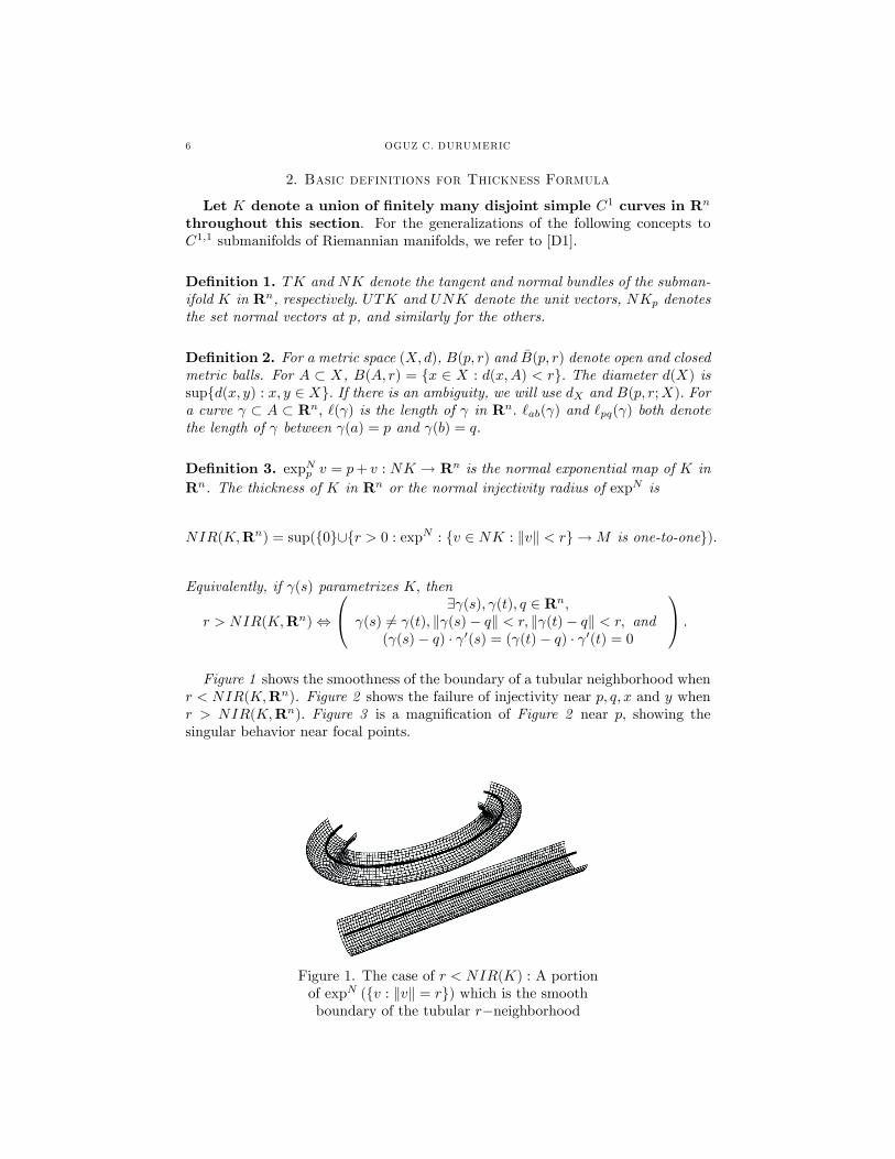
1A :Figure 1 shows the smoothness of the boundary of a tubular neighborhood when
r < NIR(K;Rn). Figure 2 shows the failure of injectivity near p; q; x and y whenr > NIR(K;Rn): Figure 3 is a magni�cation of Figure 2 near p; showing thesingular behavior near focal points.
Figure 1. The case of r < NIR(K) : A portionof expN (fv : kvk = rg) which is the smoothboundary of the tubular r�neighborhood

7
Figure 2. The case of r > NIR(K) :expN (fv : kvk = rg) is not smooth near p andq; and the failure of injectivity can be seen
around the points p; q; x and y:
Figure 3. Amagni�cation of Figure
2 near p
De�nition 4. For any v 2 UTRnp and any r > 0; de�ne
(a) Op(v; r) =[
w2v?(1)
B(expp rw; r), where v?(1) = fw 2 UTRn
p : hv; wi = 0g
or equivalently,Op(v; r) = fx 2 Rn : 9w 2 Rn; v � w = 0; kwk = 1; kx� p� rwk < rg
(b) Ocp(v; r) = Rn �Op(v; r)
(c) Op(r;K) = Op(v; r) where v 2 UTKp
(d) O(r;K) =[p2K
Op(r;K)
In all of the above, r may be omitted when r = 1: K will be omitted unless thereis ambiguity.
Intuitively, @Op(v; r) is a torus pinched at p in R3; see Figure 4: p =2 Op(v; r)which is the the open set inside the pinched torus, referred by some as a "fat torus".Op(v; r) is a donut pinched at p. Figure 5 shows a portion of @Op(v; r) and thebehavior around p:

8 OGUZ C. DURUMERIC
Figure 4. The pinched torusbounding Op(v)
Figure 5. A portion of @Op(v)
De�nition 5. (a) The ball radius of K in Rn is
RO(K;Rn) = inffr > 0 : O(r;K) \K 6= ;g:
(b) The pointwise geometric focal distance at p 2 K is
Fg(p) = inffr > 0 : p 2 Op(r;K) \Kg:and the geometric focal distance of K is Fg(K) = infp2K Fg(p): Of course, on aline segment one has Fg(p) =1 = inf ?:
De�nition 6. A pair of distinct points p and q in K are called a double criticalpair for K; if the line segment pq is normal to K at both p and q: The double criticalself distance is
DCSD(K) = inffkp� qk : fp; qg is a double critical pair for KgA double critical pair fp; qg is called minimal if DCSD(K) = kp� qk : We denotesuch a pair as MDC:
3. Shortest Curves in Rn with Curvature Restrictions
In this section, : I ! Rn denotes a simple C1 curve with a compactinterval I, k 0k 6= 0 and K = image( ); unless stated otherwise. fei : i =1; 2; ::; ng, Ei; E+i ; E
�i denote the standard basis in Rn, the ei � axis; its positive
and negative parts, respectively.
De�nition 7. For : I ! Rn, de�ne:
Dilations: dild 0(s; t) = k 0(s)� 0(t)k`( ([s;t])) and dil� 0(s; t) = ]( 0(s); 0(t))
`( ([s;t])) for s 6= t(Generalized) Curvature: � (s) = lim sup
t6=u and t;u!sdil� 0(t; u)

9
Lower curvature: �� (s) = lim supt!s
dil� 0(s; t)
Analytic focal distance: Fk( ) = (supI� (s))�1: If K is a union of �nitely many
disjoint C1;1 curves (i) in Rn; then Fk(K) = mini Fk( (i)):
Remark 3. (a) Since limv!w
](v;w)kv�wk = 1 for kvk = kwk = 1; one obtains the same � ,
if one uses dild instead of dil�, provided that k 0k � 1. The same is true for �� :(b) � (s) � �� (s);8s:(c) If 2 C1;1 and k 0k � 1; then k 00(s)k = �� (s); for almost all s.(d) lim sup
sn!s� (sn) � � (s).
Lemma 1. All of the following are equivalent for : I ! Rn with k 0k � 1:(a) � (s) � 1;8s 2 I:(b) dild 0(s; t) � 1;8s; t 2 I:(c) dil� 0(s; t) � 1;8s; t 2 I:(d) k 00(s)k � 1 for almost all s 2 I; and 0 is absolutely continuous.
Proof. (a =) c) : 8s < t < u; dil� 0(s; u) � max(dil� 0(s; t); dil� 0(t; u)): Hence, ifdil� 0(s; u) � A for some s 6= u and A; then there exists s0 2 [s; u] with � (s0) � A:
(d =) a) : k 0(t)� 0(s)k = tRs
00(u)du
� tRs
k 00(u)k du � kt� sk ; by absolute
continuity. The rest are obvious. �
De�nition 8. A C1;1 curve : I = [a; b] ! Rn is called a CLC�curve if thereexists [c; d] � [a; b] such that (a) ([c; d]) is a line segment of possibly zero length,and (b) each of ([a; c]) and ([d; b]) is a planar circular arc of radius 1 and oflength in [0; 2�). The curve need not be planar. We will use CLC(�), if theupper bound of curvature is �:
Proposition 1. Let p 2 Rn and v 2 Rn with kvk = 1:(a) 8q 2 Ocp(v);9w 2 Rn;9q0 2 @Ocp(v) and a C1 curve pq � fpg+ spanfv; wg
such that(a.i) v � w = 0; kwk = 1; and
(a.ii) pq(t) =�
p+ v sin t+ w(1� cos t) if 0 � t � t0q0 + (t� t0)(q � q0)= kq � q0k if t0 � t � t1 = t0 + kq � q0k
;
where q0 = pq(t0) and q = pq(t1); and(a.iii) pq is a shortest curve among all the continuous curves ' from p to q in
Ocp(v) with ('(t)� p) � v > 0 for small t > 0 and '(0) = p.(b) If q � p 6= �v;8� 2 R; then q0 and w are unique and pq is unique up to
parametrization. Consequently, pq depends on p; q and v continuously, if q � p 6=�v;8�:
See Figure 6 for Proposition 1.

10 OGUZ C. DURUMERIC
Figure 6. pq of Proposition 1
Proof. It su¢ ces to prove all for p = 0; v = e1 and q 6= 0; using = pq. Considerthe non-empty set of all recti�able curves ' of length � L satisfying (a.iii) for somesu¢ ciently large L < 1. Parametrize each curve ' by arclength and extend itsdomain to [0; L] by keeping ' constant after reaching q so that k'(s)� '(t)k �js� tj ;8s; t: This forms a non-empty, bounded and equicontinuous family, andlength functional is lower semi-continuous under uniform convergence. By Arzela-Ascoli Theorem, a shortest C0;1 curve from 0 to q in Oc0(e1) satisfying (a.iii)exists. The proof below will also show that we can deform any curve ' as in (a.iii)to a shorter curve until we reach which can be reparametrized to be C1: For anyu 2 Rn, de�ne uN = u� (u � e1)e1:Case 1. If q 2 E+1 ; then is the line segment from 0 to q where q0 = 0 and
t0 = 0. Furthermore, if intersects E+1 at any q00 6= 0, then q 2 E+1 : For, must
be along E+1 between 0 and q00, and then it extends uniquely as a geodesic of Rn
beyond q00 2 int Oc0(e1) to q:Case 2. \ E1 = f0g: Let w = qN=
qN ; since qN 6= 0: It su¢ ces to provethe rest for w = e2: De�ne
f : Rn�E1 ! A = fxe1+ye2 : x; y 2 R and y > 0g by f(u) = (u �e1)e1+ uN e2:
f is a smooth length decreasing map:
kf(u)� f(z)k2 = k(u � e1)e1 � (z � e1)e1k2 +� uN � zN �2
� k(u� z) � e1k2 + uN � zN 2 = ku� zk2 :
Equality holds if and only if uN = czN for some c > 0; implying u 2 span(e1; z):Parametrize with respect to arclength. Extend f � by f( (0)) = 0: By followingFederer [F], pp. 109, 163-168, we obtain that and f � are lipschitz, absolutelycontinuous, 0 and (f � )0 exist a.e., and
`( ) =
`( )Z0
k 0(s)k ds �`( )Z0
kf� 0(s)k ds � `(f( )):
Since is a shortest curve from 0 to q = f(q), k 0(s)k = kf� 0(s)k and 0(s) 2spanfe1; (s)g for almost all s 2 (0; `( )]:
( N )0(s) = 0(s)N = �(s) N (s); for s 2 (0; `( )]; a:e:
11
d
ds( N (s)( N (s) � N (s))� 1
2 ) = 0; for s 2 (0; `( )]; a:e:
By absolute continuity and (`( ))N = qN = qN e2; one obtains that �
spanfe1; e2g. This reduces the proof to the R2 case.Subcase 2.1. kq � e2k = 1, that is q 2 @Oc0(e1): De�ne
g : fu 2 R2 : ku� e2k � 1g ! fu 2 R2 : ku� e2k = 1g by g(u) = e2 +u� e2ku� e2k
:
Then, g is a distance decreasing map, kg(u)� g(z)k � ku� zk ; and equality holdsif and only if ku� e2k = kz � e2k = 1: Hence, `( ) � `(g( )), and consequently theshortest curve must lie on the circle ku� e2k = 1 between p and q, by a proofsimilar to above with f .Subcase 2.2. kq � e2k > 1, that is q 2 intOc0(e1): Any component of \
intOc0(e1) is a line segment. Let � be the component containing q. By the caseassumption and the Case 1, ��\E+1 = ;: There exists unique q0 in ��\@Oc0(e1) withkq0 � e2k = 1: By Case 2.1, is a union of a line segment and a circular arc. If were not C1 at q0 = (t0), then for su¢ ciently small " > 0; the line segmentsbetween (t0 � ") and (t0 + ") lie in Ocp(v) and have length < 2", by the �rstvariation. Hence, is C1; satis�es (a.i-iii) in R2 = spanfe1; e2g and consequentlyin Rn.Case 3. \ E�1 6= ;: Subcase 3.1. q 2 E�1 : q 2 intOc0(e1): Let � be the
line segment component of \ intOc0(e1) ending at q: Obviously, � * E�1 : Chooseq00 2 (�� fqg � @Oc0(e1)): The part of between p to q00 must be shortest also. ByCase 2, must follow a circular arc to q0 then a line segment to q00; which must bealong �: This proves (a.i-iii). By rotating around E1, one obtains in�nitely manyshortest curves � satisfying (a.i-iii).Subcase 3.2. Suppose there exists q000 2 \ E�1 and q000 6= q: Following any
� 6= from p to q000; and from q000 to q, would create a shortest curve with acorner within intOc0(e1); an open subset of R
n: Hence, Subcase 3.2 can not occur.(b) In Case 2, q0 and w are unique and is unique up to parametrization. �
Proposition 2. Let : I = [0; L]! Rn be with � � 1 and k 0k � 1: Then,(a) (s) 2 Oc (a)( 0(a)), 8a; s 2 I with js� aj � �:Furthermore, (rigidity)
( (s0) 2 @Oc (a)( 0(a)) for some a; s0 2 I with 0 < js0 � aj � �) , is a circular arc of radius 1 in @Oc (a)(
0(a)) between (a) and (s0):(b) If k (0)k = k (L)k = 1 and k (a)k > 1 for some a 2 [0; L], then L > �:(c) If 00(a) exists and k 00(a)k = 1; for some a 2 [0; L); then
8R > 1;9" > 0 such that ((a; a+ ")) � B( (a) +R 00(a); R):
12 OGUZ C. DURUMERIC
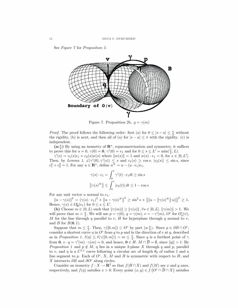
See Figure 7 for Proposition 2.
Figure 7. Proposition 2b, q = (m)
Proof. The proof follows the following order: �rst (a) for 0 � js� aj � �2 without
the rigidity, (b) is next, and then all of (a) for js� aj � � with the rigidity. (c) isindependent.(a:�2 ) By using an isometry of R
n, reparametrization and symmetry, it su¢ cesto prove this for a = 0; (0) = 0, 0(0) = e1 and for 0 � s � L0 = min(�2 ; L): 0(s) = c1(s)e1 + c2(s)w(s) where kw(s)k = 1 and w(s) � e1 = 0; for s 2 [0; L0]:
Then, by Lemma 1, ]( 0(0); 0(s)) � s and c1(s) � cos s: jc2(s)j � sin s; sincec21 + c
22 = 1: For any u 2 Rn, de�ne uN = u� (u � e1)e1:
(s) � e1 =Z s
0
0(t) � e1dt � sin s (s)N � Z s
0
jc2(t)j dt � 1� cos s
For any unit vector u normal to e1;ku� (s)k2 = ( (s) � e1)2 +
u� (s)N 2 � sin2 s + �u� (s)N u� 2 � 1:
Hence, (s) 2 Oc0(e1) for 0 � s � L0:(b) Choose m 2 (0; L) such that k (m)k � k (s)k ;8s 2 [0; L]: k (m)k > 1. We
will prove that m > �2 : We will use p = (0), q = (m), v = �
0(m), Oc for Ocq(v);M for the line through q parallel to v; H for hyperplane through q normal to v,and B for B(0; 1):Suppose that m � �
2 : Then, ([0;m]) � Oc by part (a:�2 ). Since p 2 @B \ O
c,consider a shortest curve � in Oc from q to p and in the direction of v at q; describedas in Proposition 1 : `(�) � `( ([0;m])) = m � �
2 : Since q is a furthest point of from 0; v � q = 0(m) � (m) = 0, and hence, 0 2 H: M \B = ;; since kqk > 1: ByProposition 1 and p =2 M; � lies in a unique 2-plane X through q and p, parallelto v; and � is a C1;1 curve following a circular arc of length �0 of radius 1 and aline segment to p. Each of Oc; X; M and B is symmetric with respect to H; andX intersects @B and @Oc along circles.Consider an isometry f : X ! R2 so that f(H \X) and f(M) are x and y axes,
respectively, and f(�) satis�es x > 0: Every point (x; y) 2 f�Oc \B \X
�satis�es
13
(x�1)2+y2 � 1 and (x�a)2+y2 � r2:One has 0 � r < a and r � 1, sinceM\B = ;and 0 is not necessarily on X: If r < a � 1, then the above inequalities have nosolution in R2 (by 1 � k(x; y)� (1; 0)k � k(x; y)� (a; 0)k+(1�a) � r+1�a < 1).Consequently, r � 1 < a must hold, since f(p) 2 f(Oc\B\X): For f(p) = (x0; y0);
0 � 1� r2 � (x0 � 1)2 + y20 � (x0 � a)2 � y20 = (a� 1)(2x0 � a� 1)
x0 �a+ 1
2> 1; since a > 1:
The circular part of f(�) has length �0 � m � �2 and it goes along the circle
(x�1)2+y2 � 1 starting at (0; 0). It has to follow a tangent line segment of lengthat least tan(�2 � �0) �
�2 � �0 to reach x = 1 line before f(p): This contradicts
with `(f(�)) � m � �2 ; since x0 > 1: This proves that one has to have m > �
2 ; andL�m > �
2 similarly.(a:�) It su¢ ces to prove this for a = 0; (0) = 0; 0(0) = e1 and 0 � s �
min(�; L): Suppose that (b) 2 O0(e1) for some b 2 (0; �]\ I: Then (b) 2 B(w; 1)for some unit vector w normal to e1. There is a unique c 2 [0; b) such that ((c; b]) �B(w; 1) and (c) 2 @B(w; 1): One must have ([0; c]) � B(w; 1) by part (b), since 0and (c) are in @B(w; 1) and c < �. 0(c) is tangent to @B(w; 1); since k (t)� wkhas a local maximum at t = c when c 6= 0; and c = 0 case is obvious. By part (a:�2 ), (t) must stay out of O (c)( 0(c)) � B(w; 1) for t 2 [c; c+ �
2 ]\ I; which contradicts ((c; b]) � B(w; 1): Hence, ([0;min(�; L)]) \O0(e1) = ;:Assume that 9s0 2 I with (s0) 2 @Oc0(e1) and 0 < s0 � �: Then, both (s0)
and 0 are on @B(w0; 1) where w0 = (s0)N (s0)N �1 is a unit vector normal to
e1. By part (b) and the previous paragraph, ([0; s0]) � B(w0; 1) \ Oc0(e1) whichis a circle, and (s) = (sin s) e1 + (1� cos s)w0: The converse is obvious.(c) Let q = (a) +R 00(a), and de�ne f(s) = 1
2 k (s)� qk2:
f 0(s) = 0(s) � ( (s)� q) which is lipschitz, and f 0(a) = 0(a) � (�R 00(a)) = 0;by k 0k � 1:f 00(s) = 00(s)�( (s)� q)+ 0(s)� 0(s) a.e., and f 00(a) = 00(a)�(�R 00(a))+1 < 0:Hence, lim
s!a+
1s�a (f
0(s) � f 0(a)) < 0: There exists " > 0 such that f 0(s) < 0,
8s 2 (a; a+ "). Consequently, f(s) < f(a), 8s 2 (a; a+ "): �
Example 1. The constant � in Proposition 2 is sharp. For (b), consider the partof the circle C", (x � ")2 + y2 = 1 in R2 outside the disc x2 + y2 � 1; for small": For (a), consider the LC curve in R2, which follows C" counterclockwise until itreaches ("; 1) and then the line segment [0; "]� f1g backwards to (0; 1).
Lemma 2. For all C1;1 curves : I ! Rn; analytic and geometric focal distancesare the same: Fg( ) = Fk( ) := (supI� (s))
�1: If k 0(s)k = 1 on I, then Fg( ) =
Fk( ) = (ess sup k 00k)�1:
Proof. Reparametrize to assume that k 0(s)k = 1: 1Fk( )
� � : By Proposition2(a: �2 ) and rescaling, 8p 2 ; locally avoids Op(Fk( ); ) near p and Fk( ) �Fg(p) = inffr > 0 : p 2 Op(r; ) \ g: Hence, Fk( ) � Fg( ) = infp2 Fg(p):Suppose that Fk( ) < Fg( ); i.e. sup� > 1
Fg( ): Let
A =
�s 2 I : � (s) > 1
Fg( )
�and B = fs 2 I : 00(s) existsg :
14 OGUZ C. DURUMERIC
A 6= ; and the Lebesgue measure �(I �B) = 0; by Rademacher�s Theorem.Case 1. A\B 6= ;: There exists s0 2 A\B such that c := k 00(s0)k = � (s0) >1
Fg( ): Choose r such that 1c < r < Fg( ). Let �(s) = c (
sc ); so that k�
0(s)k = 1;8s;and k�00(cs0)k = 1: By Proposition 2c, �((cs0; cs0+c")) � B(�(cs0)+cr�00(cs0); cr)for some " > 0, since cr > 1: Hence, ((s0; s0 + ")) � B( (s0) + r
00(s0)k 00(s0)k ; r) �
O (s0)(r; ): However this contradicts r < Fg( ) by De�nition 5b of Fg:Case 2. A \ B = ;: Since is C1;1; 0 is absolutely continuous, 00(s) exists
almost everywhere by Rademacher�s Theorem and k 00(s)k = � (s) � 1Fg( )
a.e.
By Lemma 1, 1Fk( )
= supI � (s) � 1Fg( )
which contradicts Fk( ) < Fg( ):Neither of the cases is possible, hence one must have Fk( ) = Fg( ). By Lemma
1, Fk( ) = (ess sup k 00k)�1 : �
De�nition 9. Let p; q 2 Rn, v 2 UTRnp , and w 2 UTRn
q be given. De�neC(p; q; v; w) to be the set of all C1;1 curves : [0; L]! Rn with (0) = p; 0(0) = v; (L) = q; 0(L) = w; k 0k � 1; and � � 1; where L = `( ) is not �xed on C:
Proposition 3. There exists a shortest curve in C(p; q; v; w):
Proof. Obviously, C(p; q; v; w) 6= ;: Any sequence of curves f mg1m=1, with `( m)!inff`( ) : 2 Cg has uniformly bounded lengths and all starting at p. Extend all m to a common compact interval by following the lines q + (s � `( m))w after q:By Lemma 1, 8 2 C, k 0(s)� 0(t)k � js� tj, and thus, C is C1-equicontinuous.C is C1-bounded by k 0k � 1. C0-equicontinuity and boundedness are obvious. ByArzela-Ascoli Theorem, there exists a subsequence of f mg1m=1 uniformly converg-ing to 0 in C1 sense: ( m(s); 0m(s))! ( 0(s);
00(s)). 0 2 C, since all conditions
of C are preserved under this convergence and `( m)! `( 0). �
Proposition 4. Let : I = [0; L]! Rn be a shortest curve in C(p; q; v; w): Then,8s 2 I; (� (s) = 0 or 1): � �1(1) is a closed subset of I, and � �1(0) is countableunion of disjoint line segments.
Proof. By the upper semi-continuity of � (Remark 3d); 8� � 1; � �1([�; 1]) is aclosed subset of I and J(�) = � �1([0; �)) is countable union of relatively opendisjoint intervals in I: Choose any � < 1; and a < b in a given component J 0 ofJ(�):Suppose that 0(a) 6= 0(b): Choose any smooth bump function h : R ! [0; 1]
such that supp(h) � [�1; 1]; h(0) = 1; andR 1�1 h(s)ds = 1: Let hn be de�ned by
hn(a+b2 ) = 1 and h
0n(s) = n[h(n(s� a))� h(n(s� b))]: Then,
limn!1
ZI
h0n(s) 0(s)ds = 0(b)� 0(a) 6= 0:
Fix a su¢ ciently large n such that supp(hn) � J 0 and �RJ0h0n(s)
0(s)ds := V 6= 0:Let "(s) = (s) + "V hn(s) be a variation of : By the First Variation formula,[CE, p6],
d
d"`( ")j"=0 =
ZI
[V hn(s)]0 0(s)ds = �kV k2 < 0
Hence, for su¢ ciently small " > 0, " is strictly shorter that :

15
For all s < t and 0 < " < 12 (sup jh
0n(u)j kV k)�1 :
dild 0"(s; t) =k 0"(t)� 0"(s)k
`st( ")� k 0(t)� 0(s)k+ " kV k jh0n(t)� h0n(s)j
(t� s)(1� " sup jh0n(u)j kV k)
� (1 + "C1)k 0(t)� 0(s)k
t� s + "C2
where Ci = Ci(kV k ; sup jh0nj ; sup jh00nj) for i = 1; 2:By Remark 3a, and since � � � < 1 on J 0; for su¢ ciently small ", � " � 1+�
2 <1; and " 2 C: This contradicts the minimality of : Consequently, 0(a) = 0(b)and 0 is constant on J 0: 8� < 1; (J(�)) is a countable union of disjoint linesegments, to conclude that (J(1)) is a countable union of disjoint line segments,and � (J(1)) � 0: �
3.1. Proof of Theorem 1. See Figures 8 and 9 in conjunction with this proof.
Figure 8. Theorem 1a, for the proof of the impossibility of the case a > 0 andc� a < �, where qt = (t)
Proof. (a) By Proposition 4, there exist maximally chosen c and d such that s0 2[c; d] � [0; L] and ([c; d]) is a line segment L0 which is a CLC�curve. There existmaximally chosen a and b such that 0 � a � c < d � b � L and ([a; b]) still is a
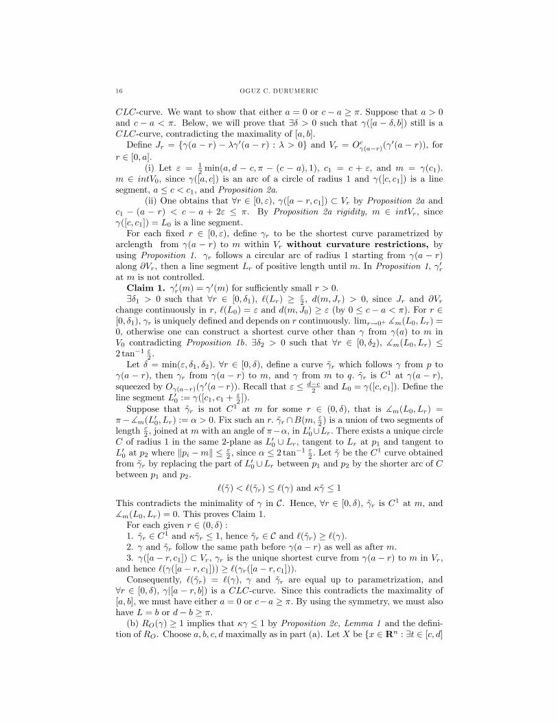
16 OGUZ C. DURUMERIC
CLC-curve. We want to show that either a = 0 or c� a � �: Suppose that a > 0and c � a < �. Below, we will prove that 9� > 0 such that ([a � �; b]) still is aCLC-curve, contradicting the maximality of [a; b]:De�ne Jr = f (a � r) � � 0(a � r) : � > 0g and Vr = Oc (a�r)(
0(a � r)), forr 2 [0; a]:
(i) Let " = 12 min(a; d � c; � � (c � a); 1); c1 = c + "; and m = (c1):
m 2 intV0, since ([a; c]) is an arc of a circle of radius 1 and ([c; c1]) is a linesegment, a � c < c1; and Proposition 2a.
(ii) One obtains that 8r 2 [0; "); ([a � r; c1]) � Vr by Proposition 2a andc1 � (a � r) < c � a + 2" � �. By Proposition 2a rigidity, m 2 intVr, since ([c; c1]) = L0 is a line segment.For each �xed r 2 [0; "); de�ne r to be the shortest curve parametrized by
arclength from (a � r) to m within Vr without curvature restrictions, byusing Proposition 1. r follows a circular arc of radius 1 starting from (a � r)along @Vr, then a line segment Lr of positive length until m: In Proposition 1, 0rat m is not controlled.Claim 1. 0r(m) =
0(m) for su¢ ciently small r > 0:9�1 > 0 such that 8r 2 [0; �1); `(Lr) � "
2 , d(m;Jr) > 0; since Jr and @Vrchange continuously in r, `(L0) = " and d(m;J0) � " (by 0 � c � a < �): For r 2[0; �1); r is uniquely de�ned and depends on r continuously. limr!0+ ]m(L0; Lr) =0; otherwise one can construct a shortest curve other than from (a) to m inV0 contradicting Proposition 1b: 9�2 > 0 such that 8r 2 [0; �2); ]m(L0; Lr) �2 tan�1 "2 :Let � = min("; �1; �2): 8r 2 [0; �); de�ne a curve ~ r which follows from p to
(a � r); then r from (a � r) to m, and from m to q: ~ r is C1 at (a � r),squeezed by O (a�r)( 0(a� r)): Recall that " � d�c
2 and L0 = ([c; c1]): De�ne theline segment L00 := ([c1; c1 +
"2 ]):
Suppose that ~ r is not C1 at m for some r 2 (0; �); that is ]m(L0; Lr) =��]m(L00; Lr) := � > 0: Fix such an r: ~ r \B(m; "2 ) is a union of two segments oflength "
2 , joined at m with an angle of ���, in L00[Lr: There exists a unique circleC of radius 1 in the same 2-plane as L00 [ Lr, tangent to Lr at p1 and tangent toL00 at p2 where kpi �mk � "
2 ; since � � 2 tan�1 "
2 : Let ~ be the C1 curve obtained
from ~ r by replacing the part of L00 [Lr between p1 and p2 by the shorter arc of Cbetween p1 and p2:
`(~ ) < `(~ r) � `( ) and �~ � 1This contradicts the minimality of in C. Hence, 8r 2 [0; �); ~ r is C1 at m; and]m(L0; Lr) = 0: This proves Claim 1.For each given r 2 (0; �) :1. ~ r 2 C1 and �~ r � 1; hence ~ r 2 C and `(~ r) � `( ):2. and ~ r follow the same path before (a� r) as well as after m:3. ([a� r; c1]) � Vr; r is the unique shortest curve from (a� r) to m in Vr,
and hence `( ([a� r; c1])) � `( r([a� r; c1])):Consequently, `(~ r) = `( ); and ~ r are equal up to parametrization, and
8r 2 [0; �); j[a � r; b]) is a CLC-curve. Since this contradicts the maximality of[a; b]; we must have either a = 0 or c�a � �: By using the symmetry, we must alsohave L = b or d� b � �.(b) RO( ) � 1 implies that � � 1 by Proposition 2c, Lemma 1 and the de�ni-
tion of RO. Choose a; b; c; d maximally as in part (a). Let X be fx 2 Rn : 9t 2 [c; d]
17
such that x � (t) ? ([c; d]) and 0 < kx� (t)k < 2g, the solid cylindrical tubewith central axis removed. Then, X � O(1; ); and hence X\ = ? by RO( ) � 1.Suppose that c� a > �: Then, ([a; d]) is a C1�concatenation of a line segment
with a circular arc of strictly more that � radian angle, contained in a unique 2plane. For su¢ ciently small r > 0; k (c� � � r)� (c+ sin r)k = 1 + cos r < 2and (c � � � r) � (c + sin r) ? ([c; d]); contradicting X \ ([0; � � c)) = ?:Consequently, c� a � �:Suppose that a > 0: Then, c = a + �; by part (a) and previous paragraph.
([0; a]) \ X = ? follows similarly. We repeat the proof of part (a) with twomodi�cations at (i) and (ii) only. At (i), choose " = 1
2 min(a; d � c; 1): At (ii) theinequality c1 � a + r � � is not needed, since 8r 2 [0; "); ([a � r; c1]) � Vr holdsby RO( ) � 1: The remainder of the proof reaches to a contradiction with themaximality of a, as in part (a) when a > 0. Consequently, the �nal conclusions area = 0 and c� a � �; and by a similar argument, b = L and b� d � �: �
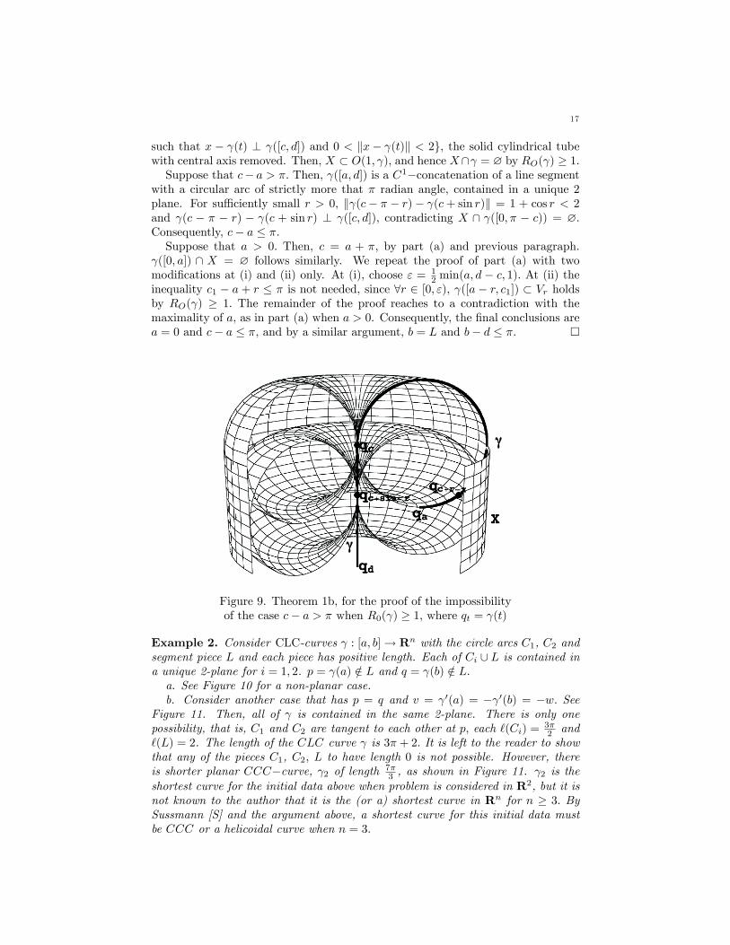
Figure 9. Theorem 1b, for the proof of the impossibilityof the case c� a > � when R0( ) � 1; where qt = (t)
Example 2. Consider CLC-curves : [a; b]! Rn with the circle arcs C1, C2 andsegment piece L and each piece has positive length. Each of Ci [ L is contained ina unique 2-plane for i = 1; 2. p = (a) =2 L and q = (b) =2 L:a. See Figure 10 for a non-planar case.b. Consider another case that has p = q and v = 0(a) = � 0(b) = �w: See
Figure 11. Then, all of is contained in the same 2-plane. There is only onepossibility, that is, C1 and C2 are tangent to each other at p; each `(Ci) = 3�
2 and`(L) = 2. The length of the CLC curve is 3� + 2: It is left to the reader to showthat any of the pieces C1, C2; L to have length 0 is not possible. However, thereis shorter planar CCC�curve, 2 of length 7�
3 , as shown in Figure 11. 2 is theshortest curve for the initial data above when problem is considered in R2, but it isnot known to the author that it is the (or a) shortest curve in Rn for n � 3: BySussmann [S] and the argument above, a shortest curve for this initial data mustbe CCC or a helicoidal curve when n = 3:

18 OGUZ C. DURUMERIC
Figure 10. A nonplanarCLC�curve
Figure 11. The shortest curve inthe plane for the p = q andv = �w initial data is a
CCC�curve, not a CLC�curve.
Figure 12. If the line segment is toolong in a U�bend (a circular arcof more than � radians), then theminimizing property may be lost:
`( 3) < `( ):
Example 3. a. The CLC�curve : [a; d]! Rn in Figure 9 (even though RO( ) <1) is the shortest curve with � � 1 and c � a � � (U-bend) for the given C1

19
boundary data at t = a and d, as long as d� c is small, by Proposition 1 (a.iii andb). However, as d�c becomes larger, some other shorter curves 3 will appear. SeeFigure 12, drawn in the 2-plane containing and 3:b. If kp� qk is large, and p� q; v; w are linearly independent, then the shortest
curves in C(p; q; v; w) will be non-coplanar CLC-curves, by studying the shortestcurves in Rn � (Op(v) \ Oq(w)) in a similar fashion to Proposition 1. See Figure10. If 0 < `(Ci) < � (no U-bends) and 0 < `(L); then the CLC-curves are expectedto be the unique minimizers.
Remark 4. a. The classi�cation in dimension 3 by Sussmann,Theorem 1 [S], im-plies the nonexistence of interior CLC sections (proper open subset) of a minimizer in C(p; q; v; w); if L 6= ?: In other words, if a minimizer contains a CLC partwith L 6= ?, then the minimizer itself is CLC with possibly longer circular arcs.We should remark that the nonexistence of LCC or CCL (with L 6= ?) minimizersin R3 are actually proved in the proof of Theorem 1 of Sussmann, even though thatis not explicitly mentioned in the statement. Hence, except the trivial cases with aline segment of length 0 in a CCC curve, see Figure 11, there can not exist anyexamples of interior CLC sections in R3. In higher dimensions, it is obvious thatC::CLC::C-curves are not minimizers (if L 6= ?), since any section CCL lies in a3-dimensional subspace, and it is not a minimizer there. However, the minimalityof other concatenations, such as helicoidal curves with CLC curves has not beenstudied in higher dimensions yet.b. Sussmann�s Theorem 2 [S] states that the helices are local strict minimizers in
R3 if the torsion j� j < 1 and � = 1: Hence, there are shortest curves in C(p; q; v; w),which do not contain any interior CLC sections. However, [S] contains some re-marks about the proof of Theorem 2, but not all details are shown.
4. Relatively Extremal Knots and Links in Rn
In this section, K denotes a union of �nitely many disjoint C1;1 simpleclosed curves in Rn and : D ! K � Rn denotes a one-to-one non-singular parametrization, where D =
Ski=1S
1(i), a union of k copies disjoint
circles, unless stated otherwise. When k 0k � 1 is assumed, S1(i) are takenwith the appropriate radius and length.A knot or link class [�] is a free C1 (ambient) isotopy class of embeddings of
: D ! Rn with a �xed number of components. Since all of our proofs involvelocal perturbations of only one component at a time, we will work with (i) :S1(i) ! Rn and we will omit the lower index (i) to simplify the notation whereverit is possible. We will identify S1 �= R=LZ, for L > 0; and use interval notation todescribe connected proper subsets of R=LZ: In other words, (i)(t + L) = (i)(t)
and 0(i)(t+ L) = 0(i)(t), 8t 2 R with
0(i) 6= 0 and (i) is one-to-one on [0; L):The following notion of ropelength has been de�ned and studied by several au-
thors, Litherland-Simon-Durumeric-Rawdon (its reciprocal was called �thickness"in [LSDR]), Gonzales and Maddocks [GM], Cantarella-Kusner-Sullivan [CKS] andothers. Cantarella-Kusner-Sullivan [CKS] de�ned ideal (thickest) knots as �tight"knots.
De�nition 10. For any : D! K � Rn , one de�nes the ropelength or extrinsi-cally isoembolic length to be `e( ) = `e(K) =
`(K)Ro(K)
= vol1(K)NIR(K;Rn) :
20 OGUZ C. DURUMERIC
De�nition 11. (a) A 0 : D ! K0 � Rn is called ideal (or thickest or tight[CKS]) in a knot/link type [ 0]; if 8 2 [ 0] with : D! K one has `e( 0) � `e( ):K0 � Rn is called ideal if any of its parametrizations 0 is ideal.(b) A 0 : D ! K0 � Rn is called relatively extremal or relatively minimal, if
there exists an open set U in C1 topology such that 0 2 U and 8 2 U\[ 0] with : D! K one has `e( 0) � `e( ): K0 � Rn is called relatively extremal /minimalif any of its parametrizations 0 is relatively extremal/minimal.
Since both length and thickness are independent of orientations and parame-trizations, we have the freedom of choosing the parametrizations to secure isotopiesand C1 convergence. We consider 1 and 2 to be geometrically equivalent, if thereexists an orientation preserving h : Rn ! Rn, a composition of an isometry and adilation (x ! �x; � 6= 0) of Rn, such that h( 1) = 2 up to a reparametrization.On each geometric equivalence class of C1;1-closed curves, le remains constant.
Lemma 3. Let : D! K � Rn be a C1 knot or link.(a) If DCSD(K) > 0; then there exists a critical pair fp0; q0g such thatDCSD(K) = kp0 � q0k :(b) If sup� <1; i.e. is C1;1, then DCSD(K) > 0:
Proof. For every sequence of critical pairs fpm; qmg with kpm � qmk ! DCSD(K),one extracts a convergent subsequence (denoted by the same index) such that pm !p0 and qm ! q0, by compactness. Then 0 = (pm � qm)� 0(pm)! (p0�q0)� 0(p0) =0, asm!1; and kp0 � q0k = DCSD(K): In order fp0; q0g to be a minimal doublecritical pair, p0 6= q0 is necessary.For (a), kpm � qmk � DCSD(K) > 0 is su¢ cient to show that p0 6= q0:For (b), dilate and reparametrize so that with k 0k = 1 and � � 1: Suppose
that pm � qm ! 0: 9m0 such that 8m � m0; kpm � qmk < 1 and pm and qmbelong the same component of K since the distances between di¤erent (compact)components of K has a positive lower bound. By Proposition 2, 8m � m0; andfor
��s� �1(pm)�� � �; (s) 2 Ocpm( 0(pm)). But qm 2 Opm(
0(pm)) since 0 =(pm � qm) � 0(pm) and kpm � qmk < 1. Hence the length of between pm and qmis � �: Same is true between p0 and q0: Consequently, kp0 � q0k = DCSD(K) >0: �
Proposition 5. Let f mg1m=1 : D! Rn be a sequence uniformly converging to in C1 sense, i.e. ( m(s); 0m(s))! ( (s); 0(s)) uniformly on D: Let Km = m(D)for m � 1 and K = (D):(a) ([CKS, Lemma 3] and [L]) If RO(Km) � r for su¢ ciently large m, then
RO(K) � r. Consequently, lim supmRO(Km) � RO(K):(b) If lim infmDCSD(Km) > 0; then lim infmDCSD(Km) � DCSD(K):
Proof. (a) The lower semi-continuity of thickness was established earlier by severalauthors, [CKS, Lemma 3] and [L], and their proofs immediately generalize to Rn:We provide a proof for the sake of completeness and to emphasize the contrast of(a) and (b), which we use repeatedly.Suppose that RO(K) < r, for a given r > 0: By the de�nition RO; there exists
a 2 D, v 2 Rn with kvk = 1 and v � 0(a) = 0 such that B( (a)+rv; r)\K 6= ;: Onecan �nd (b) 2 B( (a) + rv; r � ") for su¢ ciently small " > 0: Choose a sequencefvmg1m=1 in Rn such that 8m; kvmk = 1, vm � 0m(a) = 0; and vm ! v. Then for
21
su¢ ciently large m,
k( m(a) + rvm)� m(b)k < k( (a) + rv)� (b)k+ " < r:Hence, B( m(a)+rvm; r)\ m 6= ; and RO(Km) < r; for su¢ ciently large m; whichcontradicts the hypothesis. Consequently, RO(K) � r:(b) We will use the same indices for subsequences. Let a = lim infmDCSD(Km)
and choose a subsequence with a = limmDCSD(Km) and DCSD(Km) > 0;8m:For each m; there exists a minimal double critical pair fpm; qmg for Km, kpm � qmk=DCSD(Km): SinceK is compact and a > 0; there exists subsequences pm ! p0 2K, qm ! q0 2 K; where p0 6= q0. Since 0 = (pm � qm)� 0m(pm)! (p0�q0)� 0(p0) =0, as m!1; fp0; q0g is a double critical pair.
DCSD(K) � kp0 � q0k = limmkpm � qmk = lim
mDCSD(Km) = a:
�De�nition 12. For : D! K � Rn; (with 0 6= 0); de�ne(a) Ic = fx 2 D : 9y 2 D such that k (x)� (y)k = DCSD(K) and
( (x)� (y)) � 0(x) = ( (x)� (y)) � 0(y) = 0g and Kc = c = (Ic)(b) Iz = fx 2 D : � (x) = 0g and Kz = z = (Iz)(c) Imx = fx 2 D : � (x) = 1=RO(K)g and Kmx = mx = (Imx)(d) Ib = fx 2 D : 0 < � (x) < 1=RO(K)g and Kb = b = (Ib)
Remark 5. Kc and Kmx are closed subsets of K if it is C1;1. To show this forKc, one can modify the proof of Lemma 3. See the proof of Proposition 8, for Kmx:
This following result was proved earlier in several articles: [CKS, Theorem 7],[GL], [GMSM], It is an immediate consequence of Arzela-Ascoli theorem, and itdoes not depend on the (�nite) dimension. The existence of normal injectivityradius maximizers in �xed isotopy classes is also true in a more general case ofRiemannian manifolds by using Gromov�s Compactness Theorem, see [D1].
Proposition 6. ([CKS, Theorem 7], [GL], [GMSM]) For any knot/link class [�]in Rn, 9 0 2 [�] such that(a) 8 2 [�]; 0 < `e( 0) � `e( ); and hence(b) 8 2 [�]; (`( 0) = `( ) =) RO( 0) � RO( )) :
Proposition 7. Let f mg1m=1 : D! Rn be a sequence uniformly converging to in C1 sense, K = (D) and Km = m(D) such that 9C <1;8m; sup� m � C:(a) Let A � D be a given compact set with fs 2 D : m(s) 6= (s)g � A;8m: If
A \ Ic = ;; then 9m1 such that 8m � m1; DCSD(Km) � DCSD(K):(b) If Fk(K) < 1
2DCSD(K) and Fk(Km) � Fk(K);8m; then 9m1 such that8m � m1; RO(Km) � RO(K):
Proof. All subsequences will be denoted by the same index m. The critical pairswill be identi�ed from the common domain D:(a) Suppose there exists a subsequence m such that DCSD(Km) < DCSD(K);
8m. For all m, there exists a minimal double critical pair fxm; ymg in D for m; DCSD(Km) = k m(xm)� m(ym)k < DCSD(K): There exist subsequencesxm ! x0, ym ! y0, by compactness of D.x0 6= y0, if they are in di¤erent components of D. If both x0 and y0 2 S1(i);
then for su¢ ciently large m; xm and ym 2 S1(i): As in the proof of Lemma 3, byProposition 2, for su¢ ciently largem; the length of m between m(xm) and m(ym)
22 OGUZ C. DURUMERIC
will be at least �C . The same is true for between (x0) and (y0); to conclude thatx0 6= y0. Since 0 = ( m(xm)� m(ym)) � 0(xm)! ( (x0)� (y0)) � 0(x0) = 0, asm!1; fx0; y0g is a double critical pair for K:
DCSD(K) � k (x0)� (y0)k = limmk m(xm)� m(ym)k
= limmDCSD(Km) � DCSD(K)
Hence, fx0; y0g is a minimal double critical pair for K and fx0; y0g � Ic: Since Icand A are disjoint compact subsets of D, the subsequences fxmg1m=1 and fymg
1m=1
can be taken in D�A: 8m; fxm; ymg is a double critical pair for K; since m = on D�A:
DCSD(K) � k (xm)� (ym)k = k m(xm)� m(ym)k = DCSD(Km)
which contradicts the initial assumption. Consequently, there does not exist anysubsequence m such that 8m;DCSD(Km) < DCSD(K), proving (a).(b) By the hypothesis, Thickness formula and Proposition 5 :
2RO(K) = 2Fk(K) < DCSD(K) � limminfDCSD(Km):
Hence, 9m1 such that 8m � m1; DCSD(Km) > 2RO(K), and Fk(Km) � Fk(K);to conclude
RO(Km) = min
�Fk(Km);
1
2DCSD(Km)
�� min (Fk(K); RO(K)) = RO(K):
�
Proposition 8. (Also see [GM, p4771] for another version for smooth ideal knots.)Let K be a C1;1 relatively minimal knot or link for the ropelength `e.(a) If DCSD(K) = 2RO(K); then K� (Kc[Kmx) is a countable union of open
ended line segments, and hence Ib � Ic:(b) If DCSD(K) > 2RO(K), then K �Kmx is a countable union of open ended
line segments.
Remark 6. Theorem 2 below shows that K �Kmx is actually empty whenDCSD(K) > 2RO(K):
Proof. By using dilations of Rn, one can assume that sup� = 1: Let U be an openset in C1 topology such that 2 U and `e( ) � `e(�);8� 2 U \ [ ]:(a) As in the proof of Proposition 4, for all � � 1; � �1([0; �))� Ic is countable
union of relatively open intervals or component circles in D: Choose any � < 1 anda closed interval [a; b] contained in a component of � �1([0; �))� Ic: By repeatingthe proof of Proposition 4, if j [a; b] is not a line segment, then there exists alength decreasing variation "(s) = (s)+"V hn(s) supported in [a; b]. There existsa su¢ ciently small "1 > 0 such that 8"; 0 < " � "1; one has
1. " and belong to the same knot class and " 2 U :2. `( ") < `( ); (proof of Proposition 4 )3. � " � 1 and hence Fk(K") � Fk(K) = 1; (proof of Proposition 4 ), and4. DCSD(K") � DCSD(K) (Proposition 7(a) and [a; b] \ Ic = ;).
By the Thickness Formula, RO(K") � RO(K) and `e( ") = `( ")RO(K")
< `( )RO(K)
=
`e( ) which contradicts the hypothesis. Hence, j [a; b] must be a line segment.Consequently, Ib � Ic:
23
(b) We assume that DCSD(K) > 2RO(K) = 2Fk(K) = 2: The proof is essen-tially the same as in (a), with the following modi�cations. [a; b] is taken in anycomponent of � �1([0; �)); thus [a; b]\ Ic may not be empty. (1-3) above hold. Toconclude RO(K") � RO(K), one uses Proposition 7(b). In this case, Ib = ; andK �Kmx is a countable union of open ended line segments. �
4.1. Proof of Theorem 2.
Proof. Proof of (a) is a simpler version of (b), and we will prove (b) for a connected : D = S1 ! K � Rn �rst. By using dilations of Rn, one can assume thatsup� = 1 and consequently Fk(K) = 1; as well as k 0k � 1: Let U be an open setin C1 topology such that 2 U and 8� 2 U \ [ ]; `e( ) � `e(�):(b) By Proposition 8, there exist maximally chosen c; d such that j(c; d) is an
open ended line segment, s0 2 (c; d) and (c; d) \ Ic = ;: If d 2 Ic; then take b = d;and there is nothing to prove at this end. If d =2 Ic, proceed as follows. Assume that j[s0; d0] is a CLC-curve (in fact, a line segment followed by circular arc of possiblyzero length, that is an LC � curve) such that d � d0 < d+ � and [s0; d0] \ Ic = ;:We will show that the same is true for d0 + " for some " > 0: We point out thata priori j[s0; d0] is not known to be a shortest curve in a certain C; replacing itwith a shortest curve may create a knot outside U or the knot class of , and thisshortest curve may not have a point of zero curvature.Let fdmg1m=1 be a sequence and � > 0 be such that
1. dm+1 < dm;8m 2 N+;2. dm ! d0;3. 0 < dm � d � � < �; and4. [s0; d+ �] \ Ic = ;:
Since (s0) 2 int Oc (d0)(� 0(d0)) (Proposition 2a); (s0) 2 int Oc (dm)(�
0(dm))
for su¢ ciently large m: Let fm(s) be the unique shortest curve parametrized byarclength in C( (s0); (dm); 0(s0); 0(dm)) by Propositions 2 and 3, such thatfm(s0) = (s0) and fm(tm) = (dm) for some tm 2 (s0; dm]: Extend fm to [s0; d+�]in a C1 fashion beyond (dm) by (s� tm + dm) = fm(s):For su¢ ciently large m; �fm � 1; kf 0mk = 1 and fm(s0) = (s0): Hence, the se-
quence ffmg1m=1 is C1�equicontinuous and C1�bounded. By Arzela-Ascoli The-orem, there exists a convergent subsequence (which we will denote by the samesubindices m) fm ! f0 uniformly in C1 topology. By the construction above, f0follows past (d0) and f0(t0) = (d0) for some t0.
tm � s0 � dm � s0lim sup
mtm � d0
t0 � d0
f0(s0) = (s0) and f0(t0) = (d0)
f0 2 C1 and f 00(t0) = 0(d0)�f0 � 1
j[s0; d0] is a line segment followed by a circular arc of length at most �; andby Proposition 1, it is the unique shortest curve satisfying the last 3 conditions.Consequently, d0 = t0 and f0 = on [s0; d+ �]:
24 OGUZ C. DURUMERIC
Let m be the C1 curve obtained from by replacing j [s0; dm] by fmj[s0; tm]:Reparametrize m (not necessarily with respect to arclength) so that m(s) = (s)for s =2 [s0; d+�] and m ! in C1 sense on S1, which is possible since dm�s0tm�s0 ! 1:
Let Km = m(S1). For su¢ ciently large m � m1 :
1. m and belong to the same knot class and m 2 U :2. fs : m(s) 6= (s)g � [s0; d+ �] which is disjoint from Ic:3. Fk(Km) � Fk(K) = 1; by construction of fm:4. DCSD(Km) � DCSD(K), by Proposition 7(a).5. RO(Km) � RO(K); by Thickness Formula, (3) and (4).6. `e(Km) � `e(K); since K is relatively extremal and (1).7. `(Km) � `(K) by (5), (6) and the de�nition of `e:8. `(Km) � `(K) by construction of fm and m:9. fmj[s0; tm] and j [s0; dm] have the same minimal length in
C( (s0); (dm); 0(s0); 0(dm)):10. j[s0; dm] is a CLC-curve, by Theorem 1(a) and � ([s0; d]) = 0.
We proved that if j[s0; d0] is a LC-curve such that d � d0 < d+ � and[s0; d0] \ Ic = ;, then there exists " = dm1
� d0 > 0 such that j[s0; d0 + "] is aCLC-curve. In fact, j[s0; d0 + "] must be an LC � curve by Theorem 1(a), sinced0 + " � d < �: Hence, �0 := max f� : j[s0; d+ �] is a LC � curveg satis�es thateither d+ �0 2 Ic or �0 � �:In the case of �0 � �; (d) and (d+�) are an antipodal pair on a circle of radius
1; forming a double critical pair. This shows that 12DCSD(K) � 1: Suppose that
12DCSD(K) < 1 = Fk(K) which implies that RO(K) = 1
2DCSD(K) < 1. Theexistence of the semi-circle ([d; d+ �]) would then contradict Proposition 8a, (seeDe�nition 12). Hence, (d) and (d+�) must form a minimal double critical pair,which implies that d 2 Ic:In all cases, there exists a smallest b 2 [d; d+ �)\ Ic such that ([s0; b]) is a line
segment of positive length followed by a circular arc of length b � d 2 [0; �): Theproof is the same for the opposite direction before c:(a) Suppose that 1
2DCSD(K) > RO(K) = Fk(K) = 1: One proceeds as abovein (b) by omitting all conditions about avoiding Ic. Use Proposition 8(b), to obtainthe line segment j(c; d). Even though DCSD(Km) � DCSD(K) may not be validby Proposition 7(a), RO(Km) � RO(K) is valid by Proposition 7(b). This showsthat j[s0; d + �] is a CLC�curve, even passing through DCSD-points. (d) and (d + �) are an antipodal pair on a circle of radius 1; forming a double criticalpair. This shows that DCSD(K) � k (d)� (d+ �)k = 2 which is contrary to thehypothesis. Consequently, the case of 12DCSD(K) > RO(K) = Fk(K) = 1 with9s0 2 S1; � (s0) < sup� = 1 is vacuous.The generalizations of this proof to K with several components is straightfor-
ward, since (b) is a local result, and in (a) the existence of any s0 with � (s0) < 1leads to a contradiction. �
5. References
[BS] G. Buck and J. Simon, Energy and lengths of knots, Lectures at Knots96, 219-234.[CKS] J. Cantarella, R. B. Kusner, and J. M. Sullivan, On the minimum
ropelength of knots and links, Inventiones Mathematicae 150 (2002) no. 2, p. 257-286.

25
[CE] J. Cheeger and D. G. Ebin, Comparison theorems in Riemannian geom-etry, Vol 9, North-Holland, Amsterdam, 1975.[Di] Y. Diao, The lower bounds of the lengths of thick knots, Journal of Knot
Theory and Its Rami�cations, Vol. 12, No. 1 (2003) 1-16.[Du] L. E. Dubins, On curves of minimal length with a constraint on average
curvature and with prescribed initial and terminal positions and tangents, Amer. J.Math. 79 (1957), 497-516.[D1] O. C. Durumeric, Thickness formula and C1�compactness of C1;1 Rie-
mannian submanifolds, preprint, arXiv:math/0204050 [math.DG][D2] O. C. Durumeric, Local structure of the ideal shapes of knots, II, Con-
stant curvature case, preprint, arXiv:0706.1037v1 [math.GT][F] H. Federer, Geometric measure theory, Springer, 1969.[FHW] M. Freedman, Z.-X. He, and Z. Wang, Mobius energy of knots and
unknots, Annals of Math, 139 (1994) 1-50.[GL] O. Gonzales and R. de La Llave, Existence of ideal knots, J. Knot
Theory Rami�cations, 12 (2003) 123-133.[GM] O. Gonzales and H. Maddocks, Global curvature, thickness and the
ideal shapes of knots, Proceedings of National Academy of Sciences, 96 (1999)4769-4773.[GMSM] O. Gonzales, H. Maddocks, F. Schuricht, and H. von der Mosel,
Global curvature and self-contact of nonlinearly elastic curves and rods, Calc. Var.Partial Di¤erential Equations, 14 (2002) 29-68.[Ka] V. Katrich, J. Bendar, D. Michoud, R.G. Scharein, J. Dubochet and A.
Stasiak, Geometry and physics of knots, Nature, 384 (1996) 142-145.[L] Litherland, Unbearable thickness of knots, preprint.[LSDR] A. Litherland, J Simon, O. Durumeric and E. Rawdon, Thickness of
knots, Topology and its Applications, 91(1999) 233-244.[N] A. Nabutovsky, Non-recursive functions, knots �with thick ropes� and
self-clenching �thick�hyperspheres, Communications on Pure and Applied Mathe-matics, 48 (1995) 381-428.[M] A. A. Markov, Some examples of the solution of a special kind of problem
in greatest and least quantities, (in Russian), Soobbshch. Karkovsk. Mat. Obshch.1 (1887), 250-276.[RS] E. Rawdon and J. Simon, Mobius energy of thick knots, Topology and
its Applications,125 (2002) 97-109.[ReSh] J. A. Reeds and L. A. Shepp, Optimal paths for a car that goes both
forwards and backwards, Paci�c J. Math. 145 (1990), 367-393.[SKK] A. Stasiak, V. Katrich, and L. H. Kau¤man, Editors, Ideal Knots,
World Scienti�c Publishing, Singapore 1998.[S] H. J. Sussmann, Shortest 3-dimensional paths with a prescribed curvature
bound, Proceedings of the 34th Conference on Decision & Control, New Orleans,LA-December 1995, IEEE Publications, New York, 1995, 3306-3312.
Department of Mathematics, University of Iowa, Iowa City, Iowa 52242, Phone: 319-335-0774, Fax: 319-335-0627
E-mail address : [email protected]