INTRUSIVE MEASUREMENT EVALUATION FOR SEDIMENT-LADEN …€¦ · arrangement is suitable for studying the effect of obstacles for passing currents, and ensures the obstacle effect

INTRUSIVE MEASUREMENT EVALUATION FOR SEDIMENT-LADEN FLOWS INTERACTING WITH AN OBSTACLE

RICHARD I WILSON(1), HEIDE FRIEDRICH(2) & CRAIG STEVENS(3) (1) The University of Auckland, Auckland, New Zealand,

[email protected] (2) The University of Auckland, Auckland, New Zealand,

[email protected] (3) National Institute of Water and Atmospheric Research, Wellington, New Zealand

[email protected]

ABSTRACT

The interaction of sediment-laden flows with obstacles is a growing area of research. Sediment-laden flows are also commonly known as turbidity currents, Due to practical limitations, there are minimal experimental data available on the spatio-temporal distribution of velocity and sediment concentration fields of currents passing an obstacle. For this study, an instrumental rack consisting of an array of UVP transducers and siphons is used to measure velocity and density characteristics of turbidity currents and their interaction with a rectangular obstacle. Tests are conducted for a range of different transducer rack arrangements to determine whether their intrusive components have a significant influence on fluid flow. Lock-exchange initiated gravity currents comprised of kaolinite and glass microspheres are released in a 400 mm wide, 5000 mm long Perspex flume, filled with ambient water to an upstream depth of 300 mm. Detailed velocity contours plots surrounding the obstacle and instrument racks are obtained for each testing condition. Results show that immediately after colliding with the obstacle, the current varied in velocity distribution for all tests. It was concluded that this was likely due to the locally unpredictable nature of unsteady structures formed, rather than rack instrumental influence. Differences in velocity distributions converged to a point where all tests showed nearly identical distributions once the current head had passed the obstacle. It is therefore recommended that in future tests a recording time window of at least 20 s from collision of the current with the obstacle should be implemented. The proposed instrument arrangement is suitable for studying the effect of obstacles for passing currents, and ensures the obstacle effect dominates the signal.

Keywords: UVP, Lock-exchange, gravity current

1. INTRODUCTION

A gravity current is a density-driven, dynamic fluid process which can occur in a wide range of settings, and can be generated by geophysical or anthropogenic events. A dense fluid is released into an ambient fluid of different density. The buoyancy difference results in settling flow with an often turbulent boundary between the two fluids. In natural the marine environment, for example, such currents can be caused by buoyant river plumes along coastal margins or salty convective flows at high latitudes flowing along the seabed. A special case of gravity current occurs when the density difference is due to suspended material. These sediment-entrained gravity currents, or turbidity currents, are generally initiated from sediment failures on submarine slopes, or from rivers in flood (Meiburg Kneller 2010).Turbidity currents are an important topic due to their interaction with engineering structures. They have been attributed to causing submarine cable breakage (Heezen and Ewing 1952; Hsu et al. 2008). They are also one of the principal sedimentation processes in reservoirs, an important issue in water resources research (Fan 1986; Fan and Morris 1992).

In recent years, highly resolved three-dimensional simulations of gravity currents have been adopted to investigate the interaction of gravity currents with obstacles (Gonzalez-Juez et al. 2009; Tokyay et al. 2011; Tokyay et al. 2012). However, due to practical limitations, there is minimal experimental data available on the spatio-temporal distribution of velocity and concentration fields of currents surrounding an obstacle. In order to allow better comparisons between experimental and theoretical studies on obstacle interaction, experimental measurement techniques which capture significant amounts of flow data need to be explored in further detail. Ultrasonic Doppler Velocity Profiling (UVP) is a recent advance in velocity quantification of turbidity currents, being extensively tested by Best et al. (2001). UVP transducers record one-dimensional profiles of fluid velocity, which can be used to interpolate a two-dimensional velocity flow field when transducers form a matrix or array. The obtained data allows for flow characteristics to be calculated at a large range of points within the profile boundaries. This allows a more detailed comparison with theoretical models. Measurement of in-situ current density is useful for details such as density stratification and the ratio of internal to buoyancy forces at a given location. Using siphons to extract samples of a propagating current is a common method for finding in-situ density (McCaffrey et al. 2003; Sequeiros et al. 2010; Stagnaro and Bolla Pittaluga 2014).

2860©2015, IAHR. Used with permission / ISBN 978-90-824846-0-1

E-proceedings of the 36th IAHR World Congress, 28 June – 3 July, 2015, The Hague, the Netherlands

Whilst being able to provide a wealth of data, a detailed setup of UVP transducers and siphons in confined testing environments, such as a flume, is intrusive on fluid flow. Using these measurement techniques simultaneously introduces the question of what influence might they have on turbidity current flow structures and velocity distribution? The following paper investigates the influence of a purpose-designed array of 20 UVP transducers and two siphon racks on turbidity current flow over a rectangular obstacle in a confined flume. Lock-exchange experiments utilizing 5 UVP transducers are conducted for a range of different UVP transducer and siphon rack setups in a confined flume with a fixed initial current density.

2. METHODOLOGY

2.1 Experimental setup

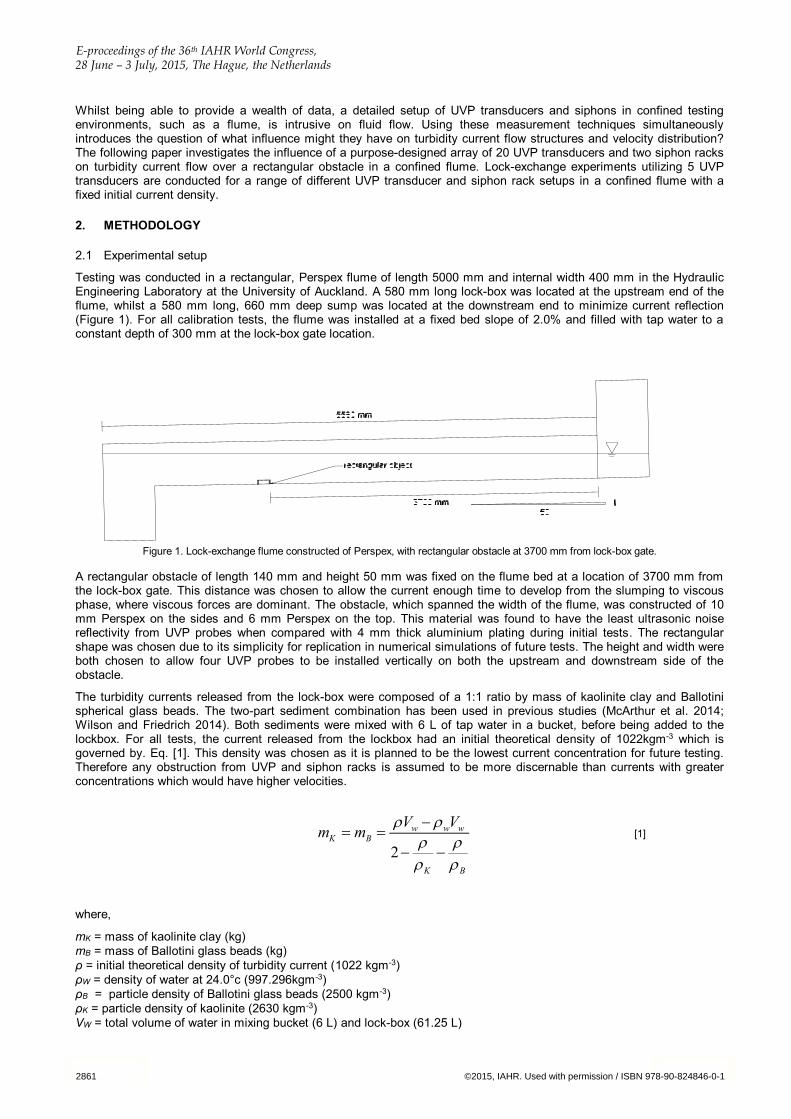
Testing was conducted in a rectangular, Perspex flume of length 5000 mm and internal width 400 mm in the Hydraulic Engineering Laboratory at the University of Auckland. A 580 mm long lock-box was located at the upstream end of the flume, whilst a 580 mm long, 660 mm deep sump was located at the downstream end to minimize current reflection (Figure 1). For all calibration tests, the flume was installed at a fixed bed slope of 2.0% and filled with tap water to a constant depth of 300 mm at the lock-box gate location.

Figure 1. Lock-exchange flume constructed of Perspex, with rectangular obstacle at 3700 mm from lock-box gate.

A rectangular obstacle of length 140 mm and height 50 mm was fixed on the flume bed at a location of 3700 mm from the lock-box gate. This distance was chosen to allow the current enough time to develop from the slumping to viscous phase, where viscous forces are dominant. The obstacle, which spanned the width of the flume, was constructed of 10 mm Perspex on the sides and 6 mm Perspex on the top. This material was found to have the least ultrasonic noise reflectivity from UVP probes when compared with 4 mm thick aluminium plating during initial tests. The rectangular shape was chosen due to its simplicity for replication in numerical simulations of future tests. The height and width were both chosen to allow four UVP probes to be installed vertically on both the upstream and downstream side of the obstacle.

The turbidity currents released from the lock-box were composed of a 1:1 ratio by mass of kaolinite clay and Ballotini spherical glass beads. The two-part sediment combination has been used in previous studies (McArthur et al. 2014; Wilson and Friedrich 2014). Both sediments were mixed with 6 L of tap water in a bucket, before being added to the lockbox. For all tests, the current released from the lockbox had an initial theoretical density of 1022kgm-3 which is governed by. Eq. [1]. This density was chosen as it is planned to be the lowest current concentration for future testing. Therefore any obstruction from UVP and siphon racks is assumed to be more discernable than currents with greater concentrations which would have higher velocities.

2w w w

K B

K B

V Vm m

[1]

where,

mK = mass of kaolinite clay (kg) mB = mass of Ballotini glass beads (kg) ρ = initial theoretical density of turbidity current (1022 kgm-3) ρW = density of water at 24.0°c (997.296kgm-3) ρB = particle density of Ballotini glass beads (2500 kgm-3) ρK = particle density of kaolinite (2630 kgm-3) VW = total volume of water in mixing bucket (6 L) and lock-box (61.25 L)

2861 ©2015, IAHR. Used with permission / ISBN 978-90-824846-0-1

E-proceedings of the 36th IAHR World Congress

28 June – 3 July, 2015, The Hague, the Netherlands

Initial tests showed that upon pouring the slurry into the lock-box, a head difference was created with the ambient water in the flume. Upon release of the gate, unwanted surges began to propagate along the flume, therefore a displacement bucket filled with water was floated in the lock-box prior to release, which eliminated the surges during gate opening. The sum of the total volume of sediment and 6 L of water in the mixing bucket was used to calculate the displacement volume required in the lock-box.

2.2 Velocity measurement and siphon positioning

Quantitative velocity measurement of the turbidity current was carried out by using a Met-Flow UVP-DUO combined with five 4 MHz UVP transducers. The transducers measure one-dimensional velocity by emitting short pulses of ultrasonic signals to a set number of virtual channels within the fluid. The virtual channels sit within a defined measurement window in line with the transducer axis, and by using Doppler theory, fluid velocity within each channel can be calculated from the shift in frequency of ultrasonic pulses reflected off microscopic particles entrained within the fluid, in which combined creates a one-dimensional velocity profile of the measurement window in front of the transducer.

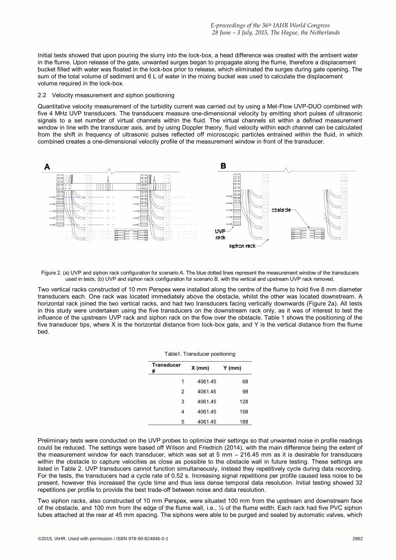
Figure 2. (a) UVP and siphon rack configuration for scenario A. The blue dotted lines represent the measurement window of the transducers used in tests; (b) UVP and siphon rack configuration for scenario B, with the vertical and upstream UVP rack removed.

Two vertical racks constructed of 10 mm Perspex were installed along the centre of the flume to hold five 8 mm diameter transducers each. One rack was located immediately above the obstacle, whilst the other was located downstream. A horizontal rack joined the two vertical racks, and had two transducers facing vertically downwards (Figure 2a). All tests in this study were undertaken using the five transducers on the downstream rack only, as it was of interest to test the influence of the upstream UVP rack and siphon rack on the flow over the obstacle. Table 1 shows the positioning of the five transducer tips, where X is the horizontal distance from lock-box gate, and Y is the vertical distance from the flume bed.

Table1. Transducer positioning

Transducer # X (mm) Y (mm)

1 4061.45 68

2 4061.45 98

3 4061.45 128

4 4061.45 158

5 4061.45 188

Preliminary tests were conducted on the UVP probes to optimize their settings so that unwanted noise in profile readings could be reduced. The settings were based off Wilson and Friedrich (2014), with the main difference being the extent of the measurement window for each transducer, which was set at 5 mm – 216.45 mm as it is desirable for transducers within the obstacle to capture velocities as close as possible to the obstacle wall in future testing. These settings are listed in Table 2. UVP transducers cannot function simultaneously, instead they repetitively cycle during data recording. For the tests, the transducers had a cycle rate of 0.52 s. Increasing signal repetitions per profile caused less noise to be present, however this increased the cycle time and thus less dense temporal data resolution. Initial testing showed 32 repetitions per profile to provide the best trade-off between noise and data resolution.

Two siphon racks, also constructed of 10 mm Perspex, were situated 100 mm from the upstream and downstream face of the obstacle, and 100 mm from the edge of the flume wall, i.e., ¼ of the flume width. Each rack had five PVC siphon tubes attached at the rear at 45 mm spacing. The siphons were able to be purged and sealed by automatic valves, which



could be opened by a remote trigger, allowing a sample of approximately 25 ml to be collected for each siphon tube. Data from the siphons is not used in this study.




Table 2. Met Flow UVP-DUO configuration parameters

Parameter Value

Sampling frequency (MHz) 4

Number of Bins 128

Bin width (mm) 1.48

Distance between bin centres (mm) 1.67

Measurement window (mm) 5-216.45

Speed of sound in water (ms-1) 1480

Velocity resolution (mms-1) 2.138

Velocity bandwidth (mms-1) 547.3

Cycles per pulse 8

Repetitions per profile 32

Sampling period (ms) 16

Full cycle time (s) 0.52

RF gain - US voltage (V) 90

2.3 Experimental procedure

In order to test the influence the upstream UVP and siphon rack had on recorded velocities of the downstream UVP rack, three different testing scenarios were chosen: (a) both vertical UVP racks, the horizontal rack and the siphon rack present (Figure 2a); (b) The downstream UVP rack and siphon rack present (Figure 2b); (c) only the downstream UVP rack present. Two identical tests were performed for all scenarios in order to check their repeatability and the influence of triggering the siphons. These tests were named A1, A2, B1, B2, C1 and C2 respectively. Scenario (a) and (b) both had siphons triggered on the first test run. The testing procedure for all scenarios began by mixing the desired sediment [Eq. 1] in a bucket with 6 L of water for at least 30 seconds. A Canon 60D was used as a reference camera. Initially, UVP recording started. Next, the displacement bucket located in the lock-box was removed, with the sediment slurry being briefly agitated again and poured into the lock box. The lock-box gate was gently opened and fastened at the fully open position, allowing the current to propagate towards the obstacle. Upon contact with the obstacle, a stopwatch was manually triggered and continued to record for 20 s where it was stopped in synchronization with the UVP transducers.

Prior to release of the current, additional UVP noise was present for all tests in scenario (b) and (c). This was likely due to lack of microscopic particles in the ambient fluid. Therefore the flume was seeded with 3 g of kaolinite before it was filled with water. The change in density of the ambient fluid caused by the seeding is thought to be insignificant.

2.4 Data analysis

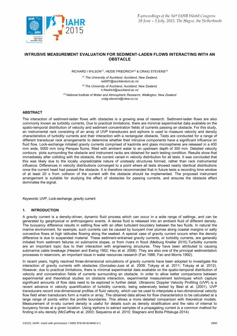
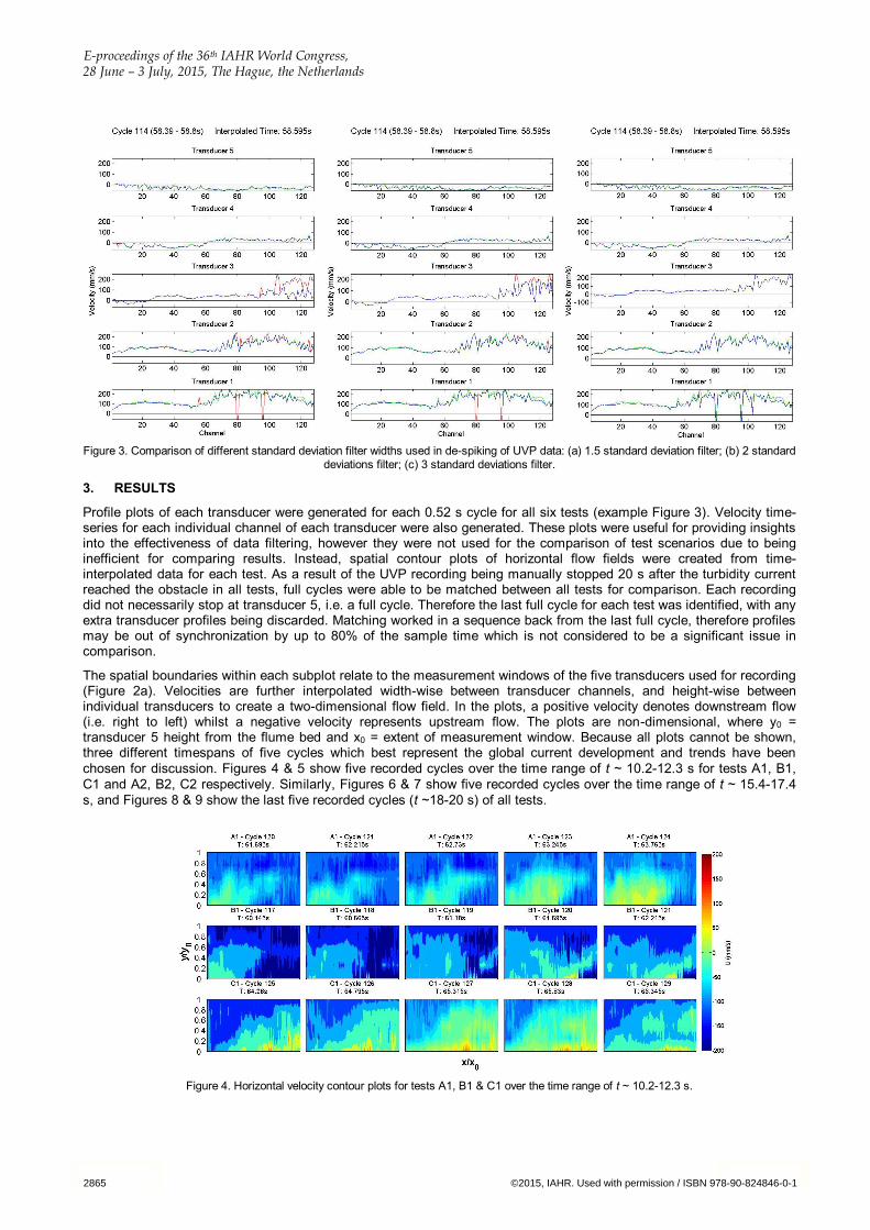
Data recorded from the five UVP transducers was processed in MATLAB through a similar procedure documented in McArthur et al. (2014). UVP velocities were first filtered for unwanted noise spikes using a de-spiking filter similar to Keevil et al. (2006). Velocities recorded from each transducer were arranged chronologically for each channel. A time-wise, 11-point moving mean was calculated along with the corresponding standard deviation. Any points which were outside a set standard deviation width were replaced by the average of the preceding and proceeding velocity. The data was processed with a limit of 1.5, 2 and 3 standard deviations, in order to find the most appropriate width. Figure 3 shows an example of filtered data from test B2, where the red line shows raw data, the green line shows spike-filtered data and the blue line shows spike-filtered and time adjusted data.

It can be seen in Figure 3(a) that 1.5 standard deviations are sufficient for eliminating spikes in the data, however it appears to also over-compensate by filtering valid data. Figure 3(c) shows that a standard deviation width of 3 appears to miss significant noise spikes, whilst a standard deviation of 2 (Figure 3(b)) appears to work best. Therefore it was chosen to apply a filter width of 2 standard deviations, which was the width also used by Keevil et al. (2006) and Wilson and Friedrich (2014).

Piece-wise cubic Hermite interpolation was applied to velocities to take into account the asynchronous nature of the UVP transducers. The filter, which has been used in previous studies interpolated an instantaneous velocity for each transducer cycle (Gray et al. 2005; Wilson and Friedrich 2014). The effectiveness of this can be seen in Figure 3, where time-interpolated velocities (green line) are identical to raw velocities for the central transducer 3, but gradually trend away from the raw velocities for the other transducers.



Figure 3. Comparison of different standard deviation filter widths used in de-spiking of UVP data: (a) 1.5 standard deviation filter; (b) 2 standard

deviations filter; (c) 3 standard deviations filter.

3. RESULTS

Profile plots of each transducer were generated for each 0.52 s cycle for all six tests (example Figure 3). Velocity time-series for each individual channel of each transducer were also generated. These plots were useful for providing insights into the effectiveness of data filtering, however they were not used for the comparison of test scenarios due to being inefficient for comparing results. Instead, spatial contour plots of horizontal flow fields were created from time-interpolated data for each test. As a result of the UVP recording being manually stopped 20 s after the turbidity current reached the obstacle in all tests, full cycles were able to be matched between all tests for comparison. Each recording did not necessarily stop at transducer 5, i.e. a full cycle. Therefore the last full cycle for each test was identified, with any extra transducer profiles being discarded. Matching worked in a sequence back from the last full cycle, therefore profiles may be out of synchronization by up to 80% of the sample time which is not considered to be a significant issue in comparison.

The spatial boundaries within each subplot relate to the measurement windows of the five transducers used for recording (Figure 2a). Velocities are further interpolated width-wise between transducer channels, and height-wise between individual transducers to create a two-dimensional flow field. In the plots, a positive velocity denotes downstream flow (i.e. right to left) whilst a negative velocity represents upstream flow. The plots are non-dimensional, where y0 = transducer 5 height from the flume bed and x0 = extent of measurement window. Because all plots cannot be shown, three different timespans of five cycles which best represent the global current development and trends have been chosen for discussion. Figures 4 & 5 show five recorded cycles over the time range of t ~ 10.2-12.3 s for tests A1, B1, C1 and A2, B2, C2 respectively. Similarly, Figures 6 & 7 show five recorded cycles over the time range of t ~ 15.4-17.4 s, and Figures 8 & 9 show the last five recorded cycles (t ~18-20 s) of all tests.

Figure 4. Horizontal velocity contour plots for tests A1, B1 & C1 over the time range of t ~ 10.2-12.3 s.




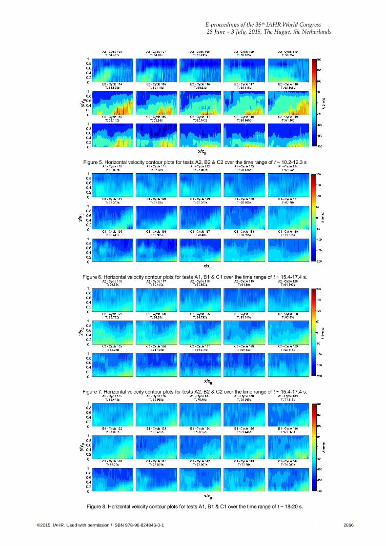
Figure 5. Horizontal velocity contour plots for tests A2, B2 & C2 over the time range of t ~ 10.2-12.3 s



Figure 8. Horizontal velocity contour plots for tests A1, B1 & C1 over the time range of t ~ 18-20 s.



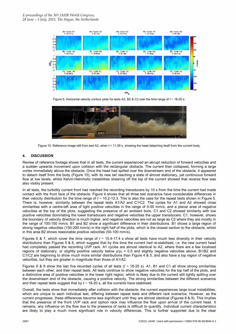
Figure 9. Horizontal velocity contour plots for tests A2, B2 & C2 over the time range of t ~ 18-20 s.

Figure 10. Reference image still from test A2, when t = 11.39 s, showing the head detaching itself from the current body.

4. DISCUSSION

Review of reference footage shows that in all tests, the current experienced an abrupt reduction of forward velocities and a sudden upwards movement upon collision with the rectangular obstacle. The current then collapsed, forming a large vortex immediately above the obstacle. Once the head had spilled over the downstream end of the obstacle, it appeared to detach itself from the body (Figure 10), with its new tail reaching a state of almost stationary, yet continuous forward flow at low levels, whilst Kelvin-Helmholtz instabilities shearing off the top of the current showed that reverse flow was also visibly present.

In all tests, the turbidity current front had reached the recording transducers by 10 s from the time the current had made contact with the front face of the obstacle. Figure 4 shows that all three test scenarios have considerable differences in their velocity distribution for the time range of t ~ 10.2-12.3. This is also the case for the repeat tests shown in Figure 5. There is, however, similarity between the repeat tests A1/A2 and C1/C2. The cycles for A1 and A2 showed close similarities with a centre-left area of light positive velocities in the range of 0-50 mm/s, and a planar area of negative velocities at the top of the plots, suggesting the presence of an ambient bore. C1 and C2 showed similarity with low positive velocities dominating the lower transducers and negative velocities the upper transducers. C1, however, shows the boundary of velocity direction is much higher, and negative velocities are not as large as C2 where they are mostly in the range of 100-150 mm/s. B1 and B2 show a significant difference in their distributions. B1 shows a large region of strong negative velocities (150-200 mm/s) in the right half of the plots, which is the closest section to the obstacle, whilst in this area B2 shows reasonable positive velocities (50-100 mm/s).

Figures 6 & 7, which cover the time range of t ~ 15.4-17.4 s show all tests have much less diversity in their velocity distributions than Figures 5 & 6, which suggest that by this time the current had re-stabilised, i.e. the new current head had completely passed the recording UVP rack. A1 cycles are almost identical to A2, where there are a few localised regions of stationary, or slightly positive velocity below y/y0 = 0.5 and slightly negative velocities above. B1/B2 and C1/C2 are beginning to show much more similar distributions than Figure 4 & 5, and also have a top region of negative velocities, but they are greater in magnitude than those of A1/A2.

Figures 8 & 9 show the last five recorded cycles of all tests (t ~ 18-20 s). A1, B1 and C1 all show strong similarities between each other, and their repeat tests. All tests continue to show negative velocities for the top half of the plots, and a distinctive area of positive velocities in the lower right region, which is likely due to the current still lightly spilling over the downstream end of the obstacle, causing a positive velocity. The strong similarities between the different scenarios and their repeat tests suggest that by t ~ 18-20 s, all the currents have stabilised.

Overall, the tests show that immediately after collision with the obstacle, the current experiences large local instabilities, which are unique to each individual test, differing between repeat tests and different rack scenarios. However, as the current progresses, these differences become less significant until they are almost identical (Figures 8 & 9). This implies that the presence of the front UVP rack and siphon rack may influence the flow upon arrival of the current head. It remains, any influence on the flow due to the presence of racks is difficult to quantify. Individual current characteristics are likely to play a much more significant role in velocity differences. This is further supported due to the clear




convergence of differences in velocity distribution as the current progresses, showing the full UVP transducer and siphon setup (Figure 2a) can be used for testing with reasonable confidence, as long as data is collected over a reasonable timeframe to allow current velocity distributions to converge.

5. CONCLUSIONS

The UVP and siphon arrangement designed to capture valuable quantitative information of a turbidity current’s interaction with an obstacle has been tested to check its influence on current flow. However, there is the potential that this instrumentation might affect the results. Analysis shows that whilst all of the tests had different velocity structures upon collision of the turbidity current with the obstacle, the UVP and siphon racks were unlikely to have had significant influence on flow, as differences in velocity distributions converged as the current progressed, becoming nearly identical in shape between all tests.

The UVP and siphon rack design shows promise in collecting a wealth of useful data for future tests, however it is recommended that transducers record for at least 20 seconds from the time the current reaches the obstacle to ensure that flow has stabilised after the passing of the head, where there is no uncertainty in the influence that racks have on flow.

ACKNOWLEDGMENTS

The authors would like to acknowledge Trevor Patrick, Geoff Kirby and Jim Luo for their assistance in the laboratory.

REFERENCES

Best JL, Kirkbride AD, Peakall J (2001) Mean flow and turbulence structure of sediment-laden gravity currents: New insights using ultrasonic doppler velocity profiling. In: Particulate gravity currents. Blackwell Publishing Ltd., pp 157-172. doi:10.1002/9781444304275.ch12

Fan J (1986) Turbid density currents in reservoirs Water International 11:107-116 doi:10.1080/02508068608686404 Fan J, Morris G (1992) Reservoir sedimentation. I: Delta and density current deposits Journal of Hydraulic Engineering

118:354-369 doi:10.1061/(ASCE)0733-9429(1992)118:3(354) Gonzalez-Juez E, Meiburg E, Constantinescu G (2009) Gravity currents impinging on bottom-mounted square cylinders:

Flow fields and associated forces. J Fluid Mech 631:65-102 doi:10.1017/S0022112009006740 Gray TE, Alexander J, Leeder MR (2005) Quantifying velocity and turbulence structure in depositing sustained turbidity

currents across breaks in slope. Sedimentology 52:467-488 doi:10.1111/j.1365-3091.2005.00705.x Heezen BC, Ewing M (1952) Turbidity currents and submarine slumps, and 1929 grand banks earthquake. Am J Sci

250:849-873 Hsu SK, Kuo J, Lo CL, Tsai CH, Doo WB, Ku CY, Sibuet JC (2008) Turbidity currents, submarine landslides and the

2006 pingtung earthquake off sw taiwan Terrestrial, Atmospheric and Oceanic Sciences 19:767-772 Keevil GM, Peakall J, Best JL, Amos KJ (2006) Flow structure in sinuous submarine channels: Velocity and turbulence

structure of an experimental submarine channel. Mar Geol 229:241-257 doi:10.1016/j.margeo.2006.03.010 McArthur JM, Wilson RI, Friedrich H (2014) Photometric analysis of the effect of substrates and obstacles on unconfined

turbidity current flow propagation. Paper presented at the Reservoir Sedimentation - Special Session on Reservoir Sedimentation of the 7th International Conference on Fluvial Hydraulics, RIVER FLOW 2014,

McCaffrey WD, Choux CM, Baas JH, Haughton PDW (2003) Spatio-temporal evolution of velocity structure, concentration and grain-size stratification within experimental particulate gravity currents Marine and Petroleum Geology 20:851-860 doi:http://dx.doi.org/10.1016/j.marpetgeo.2003.02.002

Sequeiros OE, Spinewine B, Beaubouef RT, Sun TAO, Garcia MH, Parker G (2010) Bedload transport and bed resistance associated with density and turbidity currents Sedimentology 57:1463-1490 doi:10.1111/j.1365-3091.2010.01152.x

Stagnaro M, Bolla Pittaluga M (2014) Velocity and concentration profiles of saline and turbidity currents flowing in a straight channel under quasi-uniform conditions Earth Surf Dynam 2:167-180 doi:10.5194/esurf-2-167-2014

Tokyay T, Constantinescu G, Gonzalez-Juez E, Meiburg E (2011) Gravity currents propagating over periodic arrays of blunt obstacles: Effect of the obstacle size Journal of Fluids and Structures 27:798-806

Tokyay T, Constantinescu G, Meiburg E (2012) Tail structure and bed friction velocity distribution of gravity currents propagating over an array of obstacles Journal of Fluid Mechanics 694:252-291

Wilson RI, Friedrich H (2014) Dynamic analysis of the interaction between unconfined turbidity currents and obstacles. Paper presented at the 9th International Symposium on Ultrasonic Doppler Methods for Fluid Mechanics and Fluid Engineering, Strasbourg, France,


Documents

INTRUSIVE MEASUREMENT EVALUATION FOR SEDIMENT-LADEN …€¦ · arrangement is suitable for studying the effect of obstacles for passing currents, and ensures the obstacle effect