AS '

AD-TECHNICAL REPORTUSAIRO-TR-83/2

AA

THE OATMEAL MODEL-OPTIMUM ALLOCATION 00 TEST

//EQU IPMENT/M AN POWER E-VALUATED.AGAINST LOGISTICS

INVENTO I Y

RESEARCH* ,,OFFICE

. February 1983 DEL C' .. . .A- -- CTE

ditibutl is WIIUt*L

US Army Inventory Research OfficeUS Army Materiel Systems Analysis Activity

800 Custom Hose, 2d & Chestnut Sts.Philadelphia1 PA 19106

_______________________________________3 4_ .0 110 p

Information and data contained in this document are based on the inputavailable at the time of preparation. The results may be subject tochange and should not be construed as representing the DARCOM positionunless so ipecified.

lop

rIS

UNCLAS SIFIEDSE1Cu,'%IY CLASSIFICATION OF THIS PAGE (Whoei Data Entered)

REPOT DCUMNTATON AGEREAD INSTRUcTiONSREPOT DCUMNTATON AGEBEFORE COMPLETING FORM[.REPORT NUMBER 2.GOVT ACCESSION NO. 3. RECIPIENT'S CATALOG NUMBER

I. T*ITLE (andt Subtitle) S. TYPE OF REPORT &PERIOD COVERED

THE OAT"EAL MODEL -OPTIMUM ALLOCATION OF TEST Technical ReportEQUIPMENT/MANPOWER EVALUATED AGAINST LOGISTICS 6. PERFORMING ORG. REPORT NUMSE R

7. AUTHOR(s) 6. CONTRACT OR GRANT NUMBER(0)

* Alan J. KaplanDonald A. Orr

g- PEF7ORMING ORGANIZATION NAME ADDRESS 10. PROGRAM ELEMENT, PROJECT. TASK

US Army Inventory Research Office, AMS RA 3OK NTNUBR

Room 800, US Custom House2nd & Chestnut Sts., Philadelphia, PA 19106

11. CONTROLLING OFFICE NAME AND ADDRESS 12. REPORT DATEUS Army Materiel Development & Readiness Command Fbur 93 ___

5001 Eisenhower Avenue 13. NUMBER OF PAGES

Alexandria, VA 22333 Y.WaO-NITORING AGENCY NAME & ADDRESS(if different from Controlling Office) 1S. SECURITY CLASS. (of thin ropott)

I~.UNCLASSIFIED

SCH EDULE

16. DISTRIBUTION STATEMENT (of this. Report)

Approved for Public Release; Distribution Unlimited

17. LISTRIBUTION STATEMENT (of the a~atract entered In Block 20, if dii'ferent froM Report)

I*. SUPPLEMENTARY NOTES

Information and data contained in this document are based on input avail-able at the time of preparation. Because the results may be subject to change,this document should not be construed to represent the official position ofthe US Arr' Materiel Development & Readiness Command unless so stated.

WS KEY WORD.S (Continue on reverse side it necessary and Identify by block number)

Optimal Repair Level AnalysisTest Equipment AllocationHultiechelon Stockage & Maintenance Decisionst Lo isticsto Support Availability

2& A A2'7 I"rCisths em revese f neessar ad idewty by block ninbor)

curentysophisticated multi-echelon models compute stockage quantii esfor spares and repair parts tihicb will minimize total inventory invesitnentwhile achieving a target level of operational availability. The maintenanc(pollicies yto be followed are input to the stockage models.

The ('.Optimum Allocation of Test Equipment/Manpower Evaluated AgainstLogistics'\.(OATMEAL) model will determine optimum maintenance as well asstockage policies. Specifically, it will dc.Lermine at which echelonI E'a.h

D "'1473 EDITION1 OF INOV 61 IS ONIOLETE UNCLASSIFIED

SECUIVITY CLASSIFICATrO" OFTiSPCF(wr )ttn"t

SECURItY CLAnsIFICATOW OF ThIS PAO(C(W Dom Blmted-

ABSCT(__N)

4 aintenance function will be performed, including an option for componentthrowaway. Test equipment requirements to handle workload at each echelonare simultaneously optimized.

The costs minimized include those which depend on the range, n.mb.ir,End placement of teat equipments, those which depend on whether repair isdone and where it is performed, and those which depend on the range and dollarvalue of repair parts and assemblies stocked at each echelon. The modelcalculates inventory levels and maintenance policies which will achieve theoperational availability target input by the user. It will not choosemaintenance policies that preclude achievement of the target.

Real life test cases are included which investigate the efficacy of theMIP (Mixed Integer Program) module of the model.

Ii, i

UNCLASSIFIED

SECURITY CLASSIFICATION OF THIS PAGE(fWen Data Entered)

-. I: ' r i ..,• , . " , -. x -. . - . . %. . - . , . . ..H ..

ACKNOWLEDCNNTS

Mike O'Donnel was the interface between~ model developers and reali worldrequirements. OATME.AL is in a sense a model of his interpretation of' theworld, and it was his assessment of the relative priorities of introduc~Ingreal worl! complexities which guided the level of detail includred in tho

current version of OATMEAL.

N Charles Plumeri assisted in solv~ng various problems which arost& ais thf-modelling proceeded. He wrote a Arepzocessor, the current user's guide, aile

helped ir debugging. He designed the user oriented outp'.. format.

Meyer Kotkin took part in the early discussions on model foriuulatior. at

which the basic objective of OATMEAL was determined, and use of the Tagrang-Jiapproach agreed on.

Jerry Nielson contributed significantly to the readability of this repo rt.

Accessionl For

NTIS GRA&I

DTIC TABI _oucejustificatio

DistributionIAvailability- Code~s

'Avail and/orDist Special

00% 0It.

kI

TABLE OF CONTENTS

Page

ACKNOWLE D GNETNTSS .............................................. ....... 1

TABLE OF CONTENTS ..................... la

CHAPTER 1 01 .RVIEW

1.1 Objective ............................................... 2

1.3 Test Equipment and Repair Skills ......... .......... 31.4 Inputs and Outputs .............. 6$.60 ....... ....... o. 41.5 Solution Approach..*................ ............... *. 41.6 Documentation of OATMEAL. ........ ..... 6

CHAPTER II EVALUATION OF COST AND AVAILABILITY2.1 Introduction ............... ......... .. .. ............. 9

2.2 Use of Present Value ............................. 92.3 Full Deployment Assumptions ............................... 92.4 Logistical SupportCostComponents........................ 10

2.4.1 Throw Out Costs. ...... . ............. . .... 10

2.4.2 Repair Costs: Comon Labor and Manuals ............. 112.4.3 Transportation Costs. ... .................... ...... 122.4.4 Requisition Costs .................................. 132.4.5 Stockage Costs ............ ........... .. ............ 132.4.6 Bin Costs .................... ................. .. 142.4.7 Catalog Costs .................................. ... 142.4.8 Parts Costs .................. .............. ....... 142.4.9 Backorder Costs .................................... 15

2.5 Test Equipment and Special Manpower Costs.... ........... 15

2.6 Evaluation of Operational Avai]ability .................... 16

CHAPTER III OPTIMIZATION

3.1 Introductic. ........................................ 173.2 Problem Formulation Procedures .......................... 173.3 Why Mixed Integer Programming Is Needed ................... 193.4 Mathematics of Problem Formulation ........................ 203.5 Mathematical Formalism of ORLA Model ...................... 233.6 IP Approximation ................................... . . 253.7 Relation of Supply Lagrangiai to Maintenance Policy ....... 263.8 Initial Lagrangian Selection and Treatment of Operational

Availability Constraint .............................. 26

APPENDIX A INPUTS TO OATMEAL ..................................... 31

APPENDIX B PROPERTIES OF LAGRANGIAN AND MAINTENANCE POLICIES ....... 36

APPENDIX C TEST EXPERIENCE WITH THE "A" SEARCH ..................... 39

APPENDIX D COMPUTER COSTS AND RUN TIMES ............................ 43

REFERENCES .......................................................... 46IIDISTRIBTION................ .......... .... ........ 47la

CHAPTER I

OVERVIEW

1.1 Objective

Before deploying a new veapon system, the US Army must determine how to

support the system in the most cost effective manner. Currently, sophisticated

multi-echelon models compute stockage quantities for spares and repair parts

which minimize total inventory investment while achieving a target leve]

of operational availability. The maintenance policies to be followed are inpx.t

to the stockage models.

The "Optimum Allocation of Test Equipment,'Manpower Evaluated Against

Logistics" (OATMEAL) model determines optimai- maintenatice as well as stockage

policies. Specifically, it determines at which echelon each maintenancc function

should he performed, or whether the maintenance function should be eliminated; i.e.,

it does repair vs thrmo-away analysis as well as level of repair analysis.

The costs minimized include those which depend on the range, number and

placement of test equipments, those which depend on whether repair is done and

where it is performed, and those which depend on the range and dollar value of

repa~r parts and assemlies stocked at each echelon. The model calculates inven-

tory levels and maintenance policies which will achieve the operational avail-

ability target input by the user. It will not choose maintenance policies that

preclude achievement of the target.

The objective is to achieve the target operational availability at Minimum

life cycle cost.As

1.2 Conceptualization of Maintenance

The model looks at three levels of indenture within a weapon system: cumu-

ponents, modules, and piece parts. The indenture breakdown of a home audio systelr

is depicted in Figure 1. A failure mode is defined as a system failure due to a

specific module in a specific component. All failure rates are input by failul-

mode, and maintenance allocation decisions are also made by failure mode. OA'I1EA]considers four eahelons of maintenance: (1) organizational, (2) direct stipport (1w),

(3) general support (GS), and (4) depot.

Consider maintenance on the audio system shown in Figure 1. In evcrv ca.,e

turntable failure, the audio system is repaired at ORG. If the arm mechaahir faj is,

the ORG replaces the turntable and returns the unserviceable turntable U. the D'.

2

ht

.', . . * ** - .- , "'. -%f"%' . %f .,' '..,' ",.. - "~. .r '*' .- ..-' '- . '.~ .. ,, -.... " . " .: -"- . - "'. , ,''. -'.4

At the DSU a new arm mechanism is put In, end the old arm mechanism is thrown

away. If the twtor fails, the unserviceable turntable will be evacuated all the

way to GSU for repair. After the motor is replaced at GSt', the unserviceable motor

is shipped to depot for rapair. If the needle fails, all work is done at ORG, and

the needle is thrown away.

The user may have originally designated the needle as a consumable, but

the arm mechanism as pcteztillly repairable, while the model concluded it was

not cost effective to repair the arm.

It soiw.times happens that the new module appears in two (or more) different

components. Failure rates would be i..put separately for each module applica-

tion, but the comnonality would be recognized in computing stockage and logisti-

cal costs.

Since detailed part data is not generally available in early development,the pieceparts are considered in an aggregate manner. It is ales possible to

represent a group of modules, or even components by an average module or com-

ponent, specifying how many distinct modules or components this average

representn.

1.3 Test E uipment and Repair Skills

The need to use test equipment which can be quite expensive makes the

level of renair analysis mathematically challenging. A given repair action

may require miore than -ne piece of equipment, and many different actions may

have a requirement for the same piece of equipment, It is assumed that any

piece of equipment required for fault diagnosis will also be required for

repair, so that diagosis/repair can be considered one procedure. This is

reasonable because usually a repair is not considered complete unless the

equipment used for diagnosis has performed a functional check to verify the

success of the repair.

Test equipment is labelled as either common or peculiar at each echelon.

If peculiar, only integer quantities cat, be placed at a repair facility. The

whole cost of the equipment must be considered, even though the equipment is

used at the facility only a fraction of the time. If the test equipment is

common, it is assumed that only use must be rjaid fcr; if the end item needs

1/4 of the throughput of a common piece of test equipment at the facility, it

bears 1/4 of the total cost for the equipment.

Test equipment may be needed for three different types of tepair actions:

a. Repair weapon system when it fails due to the failure of a specific

component. 3

"..

b. Repair a component when it falls due to the failure of a specific module.

c. Repair a module whenever it fails.

Repair Skills. Cost of repair including labor costs is input to the mode].

However, sometimes repair required special skills which would be new to an echelon.

The user may identify special repair skills, so that the training costs and higher

salaries are properly calculated. If a special skill is needed at DSU, but the

skill will be required for only 1/4 of a man year per year, full training costs

for one person per DSU must still be incurred. The model accounts for this just

as it properly accounts for peculiar test equipment. In both cases there is ar.

incentive to allocate maintenance so that skills and equipments are not reeded

at echelons where they will be grossly underutilized.

1.4 Inputs and Ouuts

Input consists of the type of data necessary to run a supply model such

n SESAME [10], plus additional cost and maintenance related data. The user

can also provide inputs which exclude certain types of nolutions as not feas-

ible or realistic; for example, he can specify that a certain test equipment

cannot be placed below the GSU. The maintenance data consists primarily of

test equipment and special skill requirements for each maintanance action.

There can be up to four supply and maintenance echelons allowed. It Is

assumed supply and maiutenance functions are colocated, but an intermediate

A echelon can be specified to have only a maintenance function.

Replacement task distributions and maintenance task distributions [11]are outputs of OATMEAL hereas they would be input to supply models. Ai ite.',replacement task distribution gives the percent of removals which occur at each

echelon, while the maintenance task distribution specifies the percent of remove'd

items which can be repaired at each echelon.

Other outputs of OATMEAL are the numbers and locations of test equioment

and special personnel, and the stockage quatities associated with the main-

tenance policy chosen.

1.5 Solution Approach

The heart of OATMEAL is a mlxted integer program (MIP) mode Consider th

approach to solution to conasst of four stages - prepLice: sng, formulatio.n,

optimization, and evaluatior. The solution flow is depicted in Figure 2.

Preprocessor. This pro,;ram [8] accepts input from the user in a format

4

designed to be as convenient es possible. Default values for inputs are pro-

vided whenever it makes sense to do so, and there are edit checks. The output

is a parsimonious set of parameter and variable values neceasary to describe

the problent mathematically.

Formulator. This program formalates the problem as a MIP model in the

srecific format for the commercial software package being used (see below).plcvever, to do this, it must first genrnte stockae (and cost implicathon

thereof) for all candidate maintenance policies. The Formulator uses the SESAME

mult echelon stockage model [5] as a subroutine to calculate optixrally quantities

of comoonents and modules for a particular mcintenance policy vector. By policy

vector wo mean an assignment, for each failure mode, of where to replace and where

to repair the respective components and modules. The associated stockage costs

will then be accessible to the MIP cost function formulation.

Optimizer: The "HIP" refers to the commercial software package which

accomplishes the optimization. Packages for accomplishing MIP are available, each

of which required many man years to develop, The specific package now being used

is APeX [II, (1], developed by Control Pats Corporation, but others, such as TBM's

NPSX, can le substituted with little change.

MIP "optimizes"-- finds the maintenance policy vector which

minimizes costs, including stockage costs and backorder penalty costs - by using

a7. efficient heuristic search so that all the nyriad combinations do not have

to be evaluated.

Eveluator. As the name implies, this propram evaluates; it accepts as input

all the data about the problem being run and also a maintenance policy vector

(the replace-repair actions by failure mode) to be assessed in terms of cost and

performance. This policy vector may have come from the optimizer or been proposed

by the user (note alternative policy block in Figure 2). The evaluator uses

SPSAME subroutine to determine for each component and module the optimum stockage

quantitie . The evaluator will determine the operational availability performance

based on the computed stockage quant.ties and the selected maintenance policy

vector; it also will compute all relevant costs (see Chapter 2 for cost elementsand expressions). Finally the evaluator will convert the failure mode policy

vector to component and module replacement task distributions and maintenance

task distributions (Section A.8.4).

OATrEAL, by incorporating SESAME model subroutines, simultaneously optimizes

maintenance and supply, IE SESAME or a comparable stockage optimikcr is

5

"I

not included in a repair level analysis model, estimates of the Impact of different

maintenance policies on stockage costs cannot bL correctly estimated. Therefore,

this may result ir the choice of maintenance policies which are not as cost effec-

tive as expected. This phenoenon will be most pronounced when the raintenance

policies have an adverse impact on operational availability, requir.-rLg a very

large investment in inventory to cospensatw.

1.6 Documentation of O&TEA L.

The User's Guide (83 explains in detail the input required from the users,

default parameters, the interpretation of output, and different approaches t,

using the OATWIAL model for maximum benefit. It also documents the transforma-

tions made by the pre-processor to develop the inputs required by the MIP foxmu-

intor.

This report is Intended for a range of readers with different objective5.

This Chapter, Chapter i and Sections 3.1-3.3 of Chapter III do not require a

sophisticated mathematical background, and are intended to give analytically

inclined readers a good understanding of the capabilities of the model. Chapter

II describes how the model evaluates costs and operational availability. Chapter

III discusses the elements of the optimization process, i.e. the MIP formulation,

selection of a backorder penalty parmeter, and evaluation of the cost-availability

performance for maintenance policy vectors.

I6i.

~16.4

, ; . , ,, , .. .. . .. ..o . . ,.. . . .. .. . , . .. .. - . .. -.o*,.,* .- '. - -. -'. - ,." " ... , .. , ..' '-'- - - " " ," . , ', . ,. . - . . " .' . ,, .

4n CieJ

uJL

Ing

I'C

Lai

Lia:

L aJuIL !s84

L) I .L-s-a LL ujao

CD-

0-~~ 8,LLL*i

oil

w CL

-4I

Lb-.

w C)

LU LU15>w~

In( .- u

&n ILiecr

08C aw u-

CL~cz

LWA

CHAPTER I

EVALUATION OF COST AND AVAILABILITY

2.1 Introductiou

This chapter will give the reader the scope of the costs considered, the

actual cost equations, and an idea of how performance is evaluated through end

item availability. A more mathematical treatment of the functional details of

OATMEAL is left to Chapter III.

2.2 Use of Present Value

Because 0ATWEAL's objective is to minimize life cycle costs, the costs con-

sidered are a mixture of one-time costs and recurring annual costs. To make

these two types of costs commensurable, the present value approach as recom-

mended in DoDI 7041.2 [12] is used.

As an example, given that:

a. 100 requisitions are processed per year.

b. Cost per requisition processed is $10.

c. Expected lifetime for the system is 11 years.

d. Discount rate for present value analysis is 10%.

Then, assuming coste are incurred at midyear,

3.1 t-1/2Requisition Costs (Present Value)- ($10) x (100) x

t-l

This may be rewritten as:

11 t-1/2Requisition Costs (Present Value) - ($10) x (100) x E (-0)

t-1

- Annual Requisition Costs x PVFAC

where PVFAC - present value adjustment factor. Note that PVFAC depends only on

the expected life of the system and the discount rate, and can be used to con-

vert other annual costa to the present value of expected lifetime costs. While

PVFAC may be calculated as shown, it is input to OATMEAL from the pre-processor,

which takes the correct value from official DoD tables.

2.3 Full Depl.ypent Asmptions

Full deployment is assumed in year 1. This means cost estimates produced

9

..............-. - - - - - -

are not true life cycle costs, but are useful. for ranking policy alternatives,

This approach was taken to simplify data requirements and processing with the

expectation that this would not unduly bias choice of one alternative over

another. It does tend to exaggerate the impact of costs which will phase in

over -tme, so nome refinements may ultimately be neces3ary, e.g., a factor

applied to PVTFAC. Note that not only do annual costa such as requisition pro-

cessing build up to Pull deployment levels, but even "onetime" costs such as

purchase price for test equipment, are not really all incurred at one time;

test equipment, for example, need only be deployed as the weapon system is

introduced over time to additional fighting units.

2.4 Logistical Support Cost Cooenants

Costs are computed for each individual component and module using the equa-

tions described. The variables underlined in the equations are passed directly

from the preprocessor. The other variables are computed or modified by OATMEAL

and depend on the maintenance polieies chosen.

2.4.1 Throw Out Costs

Throw out costs represent the annaal value of the components and modules

which wash out and must therefore be replaced by new procurement. As with all the

other annual costs, PVFAC is used to convert the estimate of annual costs to the

present value of expected lifetime throw away costs. It is assumed that the

administrative costs of making procurements will not significantly vary among

alternative maintenance policies and need not be considered.

Mathematically, the equation for throw out costs for any given component

or module is:

THROW OUT COST - PVFAC z (Annual Removals) x (Z Washout) x (Unit Price)

Annual removals reflect failure rates plus "false" removals. A "false"

removal occurs when a component or module which is perfectly good Is removed due

to an error or ambiguity in diagnosis. Currently, the model user inputs a failure

rate for each failure mode, but a single false removal rate which applies to all

items. If the false removal rate is 10 percent and a component or module is ex-

pected to fail 100 times a year, total removals are estimated as (100 + 100 x 10%)

or 110.

Maintenance policies impact removal rates in that if a component is thrown

10

, ..fj. -

out rather than repaired, this will eliminate demand for modules used to repair

that component. Throv out costs are cumputed fc the component, since each com-

ponent thrown out must be replaced by procurement, but no throw out costs are

computed fur its modules.

At, inherent washout rate is input for each component and module, reflecting

the percent of removals which cannot be fixed regardless of the maintenance

policies chosen. If a throw out policy is selected by the model, or input for

evaluation, the washout rate becomes 100 percent.

2.4.2 Repair Costs: Common Labor and Manuals

Repair costs include labor, parts, and the need to develop repairmanuals. Two types of labor are considered, common and special skills. Thereason for treating special skills separately is that just as peculiar test

equipment, they may not be fully utilized; e.g.,, if repair requiring a specialskill is done at ORG, the full cost of putting the specially trained person at

ORG is incurred even though he may need to use his special skill only a small

portion of the time. Special skills costs are discussed further in Section 2.5

while parts costs are discussed ix Section 2.4.8.

While special skill requirements are treated in detail, common labor costs

are treated somewhat approximately in order to simplify the data requirements

of the model. The user inputs ths average hours of labor to repair each component

and each module. He does not enter the hours to repair the end item itself, or

relate the number of hours to repair a component to the failure mode. Thus,

common labor repair costs are computed per component or per module repair action.

Because of differences in pay scales and working hours by echelon, the same

joL will incur a different cost depending on the achelon at which it is done.

The pre-processor takes all this information into account and inputs to OATMEAL

the cost per repair action by echelon. The number of repair actions per echelon

is then computed by the EVALUATOR from the annual removals and the maintenance

task distribution.MTD i defied an the percent of all removals (no matter where emoed)

repaired av lon k, where k takes on the values 1, 2, 3 and 4 to refer

respectively to the ORG, DSU, GSU and depot repair echelons (e.g. MTD3 is percent

of all removals repaired at GSU). The sum of MTID. + MTD + MTD3 + MTD4 plus the

washout rate will always equal 100 percent.

11

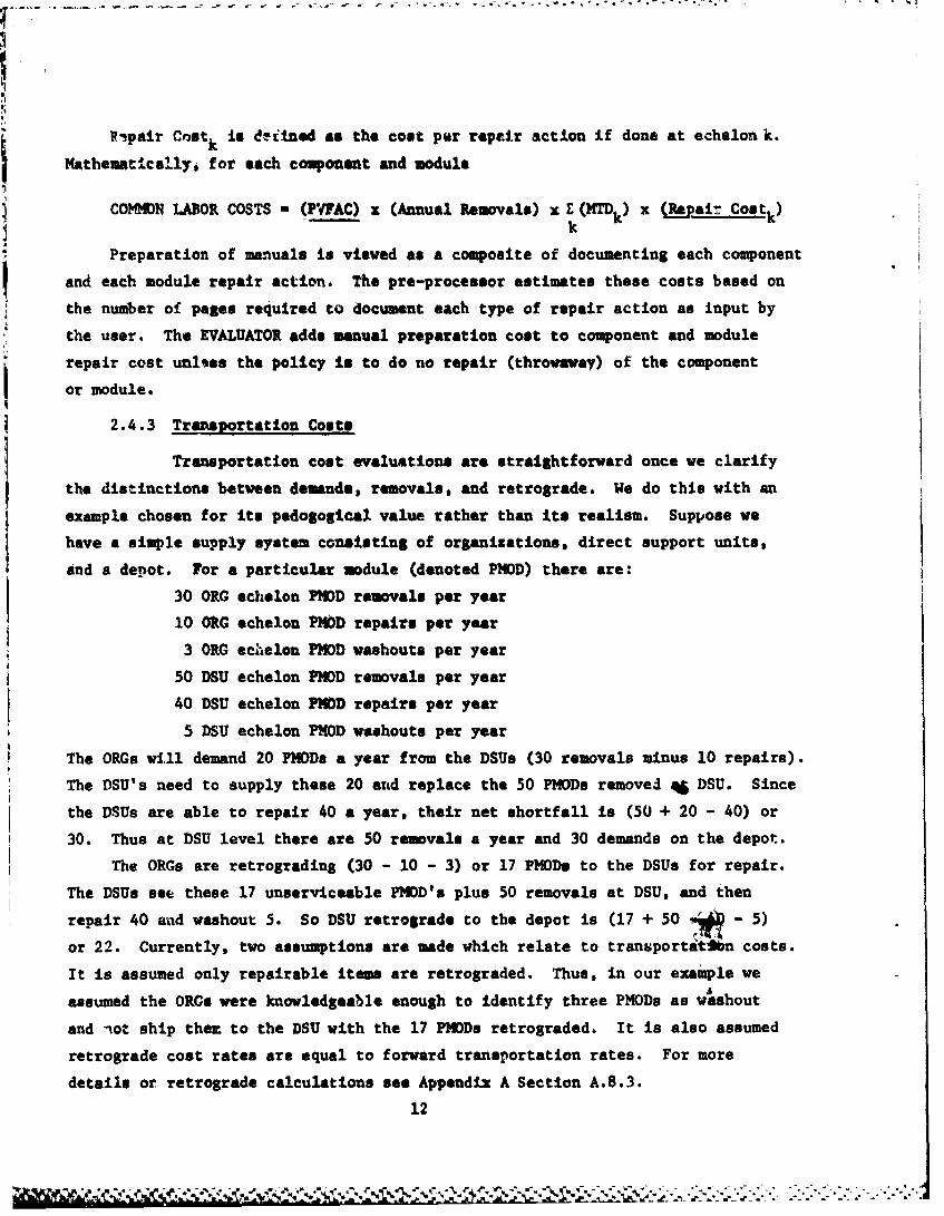
Vipair Cnatk is d-itned as the cost per repair action if done at echelon k.

Mathematically, for each component and module

COHMMN LABOR COSTS - (PFAC) z (Annual Removals) x E (MTDk) x (RMpair Costk)-- k

Preparation of manuals is viewed as a composite of documenting each component

and each module repair action. The pre-processor estimates these costs based on

the number of pages required to document each type of repair action as input by

the user. The EVALUATOR adds manual preparation cost to component and module

repair cost unlass the policy is to do no repair (throwaway) of the component

or module.

2.4.3 Transportation Costs

Transportation cost evaluations are straightforward once we clarify

the distinctions between demands, removals, and retrograde. We do this with an

example chosen for its pedagogical value rather than its realism. Suppose we

have a simple supply system consisting of organizations, direct support units,

And a depot. For a particular odule (denoted PMOD) there are:

30 ORG echelon PHOD removals per year

10 0RG echelon PMD repairs per year

3 ORG ecielon PMOD washouts per year

50 DSU echelon PMOD removals per year

40 DSU echelon POD repairs per year

5 DSU echelon PMOD washout. per year

The ORG will demand 20 PMODs a year from the DSUo (30 removals minus 10 repairs).

The DSU's need to supply these 20 and replace the 50 PMODs removed 6 DSU. Since

the DSUs are able to repair 40 a year, their net shortfall is (50 + 20 - 40) or

30. Thus at DSU level there are 50 removals a year and 30 demands on the depot.

The ORGa are retrograding (30 - 10 - 3) or 17 PMDo to the DSUs for repair.

The DSUs see these 17 unserviceable PMOD's plus 50 removals at DSU, and then

repair 40 and washout 5. So DSU retrograde to the depot is (17 + 50 - 5)

or 22. Currently, two assumptions are made which relate to transportattbn costs.

It is assumed only repairable items are retrograded. Thus, in our example we

assumed the ORCe were knowledgeable enough to identify three PMODS as washout

and not ship them to the DSU with the 17 PMODs retrograded. It is also assumed

retrograde cost rates are equal to forward transportation rates. For more

details or retrograde calculations see Appendix A Section A.8.3.

12

-.- ,, ,,. ; ,;. ,,,,.-,-L, -,.,;-,;%;:..'..,., ... .,,. . .,: . , -;..: :....<--.:.- .:.-.. .:.:.-.............

II',

The reader can see@ from the example given, that the maintenance policies,

by affecting where repair is done, - both emand and retrograde. Let

Annual Demandk denote the total demands placed by echelon k sites on theirsuppliers and Transport Ratek denote the cost per pound of moving material

from supplier to echelon k. Analogously, Annual Retrogradek and Retro Ratek

refer to movement from echelon k to the maintenance units providing support.

Then,

TRANSPORTATION COST -

* PVFAC x (Item Weight) x E (Annual Demandk) x Transport

+ PVFAC x (Item Weight) x r (Annual Retrogradek ) x (Retro Ratek )k

2.4.4 Requisition Costs

Annual Requisitionsk is defined as the number of requisitions for

a given component or module placed annually by echelon k sites vn their suppliers.

One-for-one ordering is assumed for the most part, i.e. each item demanded results

in an additional requisition. However, this is qualified to the extent that it

is assumed no single site will requisition the same item more than 12 times a

year. Thus, for low demand items, number of requisitions equals number of demands,

but not for high demand items, for which Annual Requisitionsk may not exceed 12.

Mathematically,

REQUISITION COSTS - PVFAC x E (Annual Requisitinns ) x (Requisition Cost Parameter)k

2.4.5 Stockaae Costs

Stockage costs include the one-time costs of buying stock to fill

the pipeline, and an annual holding cost to cover stockage and losses or pilferage

of inventory. One issue is: what is the impact on cost of engineering redesignwhezeby better performing components or modules replace those previously used?

Will the new item simply be bought when it is time to replenish washouts of the

old item, or will all stocks of the old item be excessed at time of engineering

redesign, increasing cost? A second issue is: Can pipelines be drawn down

gradually so that if, for example, phase out begins in 1994, procurements to

replace washouts after 1994 are avoided by using stocks in the pipeline, saving

money?

13.4

To simplify data requirements the issues raised are avoided by not including

either excess costs, or cinge from pipeline veductions. Lattir 8 HCFAC be the

annual cost of storage and pilferage, as a percent: of unit price:

STOCKAGE COST - (Quantity Stocked) x (Unto Price) +

PVFAC x (Quantity Stocked) x (Unit Price) x HCFAC

2.4.6 Bin Costs

Bin costs are those management and holding costs which vary as a

function of the range of items stocked rather than the dollar value or quantities

stocked. The bin cost parameter is the cost per NSN per stockage location per

year so that for each component or module:

BIN COST - PVFAC x (Number of Stocking Locations) z (Bin Cost Parameter)

Bin costs and stockage costs are the two cost components that depend on theanswers found by the SESAME subroutines of OATMEAL as to how much and where to

stock components and modules.

2.4.7 Catalog Costs

Each module and component is coded as to whether it is a new item or

not. If it is new, a one time catalog introduction cost is incurred; additionally

a recurring maintenance cost is assessed.

Therefore,

CATALOG COSTS - (Total New Items) x (Item Introduction Cost) +

PVFAC x (Total New Item) x (Item Maintenance Cost)

2.4.8 Parts Costs

For each module an average part is created to represent all parts

used in fixing the module. The unit price to be used for the average part is

calculated by the pre-processor based on the average val.e of parts used per

repair action. Demand is estimated as the total demand for the module, less module

washouts divided by the number of parts the average represents. The echelons

at which demand arises are inferred from the echelons at which the module is

repaired.

*

The number of parts is actually based on new parts only. This means demand forold parts is attriLuted to new parts so that added stockage costs for old partsare reflected as added cost for new parts.

14

Once the average part is described, SESAME subroutines are used to calculate

stockage and all logistics costs are calculated including throwaway (washout is

alwa~s lO percart), tequisitioning cost, stockage cr t and bin cost. These costs

are mltiplied by the number of parts the average represents. The number of new

parts introduced contributes to cataloging costs.

2.4.9 Backorder Cc-ts

Component backorders degrade operational availability, while module

backorders increase the number of components in the repair pipeline. Ideally,

these increased pipelines would be acznunted for in computing component stockage.

Neither SESAME nor the OATMEAL model currently does this. Therefore, the back-

orders themselves are costed out. If module backorders will increase the number

of covponents in the pipeline by n, and each component costs UP, module backorders

are costed out as (n) x (UP).

By analogous reasoning, parts backorders are costed out in terms of the

increase in the expected number of modules in the repair pipeline.

2.5 Test Equipment and Special Manpover Costs

For each type of test equipment and each different kind of specially tra ed

repairman, the EVALUATOR calculates the total requirement and multiplies by the

cost per equipment or per repairman which is input. The pre-processor bases

test equipment cost on purchase price, installation cost, and an annual main-

tenance cost expressed as a percent of purchase price. It -Jso checks to see if

the test equipment life is les then the weapon system's life, in which case itincludes a cost to reflect the need to eventually replace the test equipment.

The pre-processor bases repairman costs on salary and training cost; annual

training cost is the cost of training divided by the average length of time a

repairman stays in his position. Repairman cost may vary by echelon

OATMEAL calculates workload on equipmnt or special repairmen in detail.

Workload factors are input to the EVALUATOR by failure mode for end itat, and

component repair; i.e. workload to repair the end item may depend on which

component failed, and workload to fix the component may depend on which module

failed. Module repair workloads do not depend on which component the module camE

from, nor does the user, in developing input to the pre-processor, necessarily

Actually, to be consistent with calculation of stockage cost, we use(n) x (UP) + (PVFAC) x (n) x (UP) x (HCFAC).

15

- - - - - .-. . - - -

have to use the capability to make component an4 end item repair workloads depend

on failure mode.

Equipment and ripairmen requr 'nts are calculated by site, reflecting

the workload factors, fquipmants r.,,rted by the site. and the mainten2nce

policies. If the equimont. or repairman will be at the site just to support

the sinSle weapon system, i.e. it iu peculiar to the weapon system, requirements

are rounded up: 2.2 becwms 3 and so on.

2.6 Evaluation o. Operstiol Avaitlbility

O'eraticual availability Is astinated as:

OA a NCTINCTU + )MTR + arT + MT

.4 where

OA - operational availability of the weapon system

NCTII - mean calendar tim between faxlures

Mr - mean time to repair the weapon system if all resources are

available

TT - mean transportation time

ELDT - man logistics down time

CTBF and M are inputs and relate to the performance of the weapon system

independent of what support it receives.

4TT In a function of the repair level decisions. If the yatesm Is always repaired

at user level with user personnel and equipment, MTT equals 0. Otherwise, MITT

covers the tim for the upper echelon personnel to get to the user, or for the

system to be moved to the repair site and back.

ELDT is the mean time to get an essential component from the supply system

when needed for weapon system repair. It depends on the repair level analysis

in that for any given set of maintenance policies, there is an associated set of

stockage levels, and the EDT is a function of these supply levels and the

maintenance policies. The SESAICE stoakage model calculates LDT.

16

.4 4 .

Mx-

'a ~ - --- ---.-.- - -~ - - - - - - - -

OPTIZATION

3.1 Introduction

This chapter discusses the mathematics and procedures for problem formula-

tion and optimiation.

One difficulty encountered relate& to the need to use SESAME in problem

formulation. To compute stockage, SESAME must first find the value of a

Lagrangian (called CURPAR In the SESAME literature) by which stockage is related

to the operational availability target. Unfortunately, SESAME cannot find the

Lagranoian without first knowing what maintenance aJ.location decisions will be

made.

Thus, there is circularity: opttmimum maintenance allocation decisions

depend on stockage costs, while the computation of stockage quantities require

that CURPAR be known, and CURPAR epends on what the maintenance allocation de-

cisions are. In Sections 3.5 and 3.6 we describe the circularity and how we

circment it ia detail. U.itt.l then the reader is asked to accept thet SESAME

can compute &cockage in the problem formulation stage.

3.2 Priblem Formulation Procedures

As itated in Casuer 1, OA.1UKAL considers three levels of indenture and

four echelons of maintenar .e (plu throw-away). This structure would generate

53 possible maintenaire, policies for ench failure mode. Powever, OATMEAL re-

quires that a modtle be repaired at the same or higher echelin as the component,

and the component repaired at the sme or higher echelon as the end item.

Further, sd item repair is limted to ORG o: DS, resulting in 25 possible

maintenance task a~loca4iors for aih 9ailure mode. These policies can be ex-pressed as a triplet In which the first variable states the echelon for end Item

repair, the second, component repair, and the third, module repair (see Table 3.1).

In particular cas. some of the 25 may be excluded by the user. Although the

optimization examines 25 maintenance policies for %ach failure mode, the formu-

lator does not. Instead, the costs for these policies are built up from the

costs found for zomponents and modules considered Individually. Thus, in computing

stockage, the formulrtor applies SESAME to each of nine alternatives for each

component and to each of 15 alternatives for each module.

17

.4t

9L .-

COW, ONMI ALTERRATIVR S

() (2) (3) (4) (5) (6) (7) (s) (9)REPLACE 0ftc OltG OROG ORC ORG DSU DSU DSU DSU

AZ.PAItl On. DSU ON Delpot Tht,w DSU GSU Depnt ThrowAway Away

.TABLE 3.1. POLICY NM, TABLE

I.-I

1PI O 01 2 DSU 3S "eo TSh 4 DSUO 5 "e~ Throwy

3AL 3 *PLC NMU ALPoiicy Nquiber lRd tinl Impair Couent lRepair Module ltepair

2 1 1 2

4 1 1 4

s 1 1 5

6 1 2 2

7 1 2 3

8 1 2 4

9 1 2 5

10 1 3 3

11 1 3 4

12 1 3 5S13 1 4 4

14 1 4 5

15 1 5 5

16 2 2 2

17 2 2 3

18 2 2 4

19 2 2 5

"4 20 2 3 3

21 2 3 4

22 2 3 5

23 2 4 4

24 2 4 5

25 2 5 5

18

.W?

The following example shows how the formulator derives failure mode coats

froim cost, for Individual components and modules.

Logistics Costs for Component 1

For ORG Resmoval/DSU Repair $100

For ORG Removal/1epot Repair $140

Logistics Costs for Module 1

For DSU Remova/Throws:ay $ 50

For Depot Removal/Throwaway $ 30

Failure Mode 1

Defined as Failure of Nodule 1 Causing Failure of Component 1

Accounts for 401 of Component 1 Failures

Accounts for 802 of Module 1 Failure (this Implies module 1 in in

some other component besides component 1)

Logistics Cost for Failure Mode 1

Policy Coat

OAS Reuoval/DBU RepAIr/rModule Throwaway (401)($100) + (8O) ($50)

ORG Resoval/Depot Repair/Module Throwaway (4O) ($140) + (802) ($30)

3.3 Why Mixed Intaer lrograma Is Needed

The procedure just outlined develop* the logistical cost' impact of each

miutmence alternative for each failure mode. The least cost set of alternatives

is readily identified. If this set Is implmented, however. test equipment

(and special repair skills) costs could be excessive because no effort has been

made to place all maintenance functions which use the am equipment at as few

sites as possible. Conversely, If policies are selected simply to minimize

test equipment costs, logatical costs may become excessive. If each piece of

equipment were used for just one failure mode. we could Include test equipment

costs In with logistical costs in choosing the policy alternative for that mode.

When test equipment has many uses, however, we can no longer select the policy

for one failure mode Independently of the policies we choose for other failure

modes.

A successful approach to doing repair level analysis with shared test

, oequipment has been developed and Implemented by the US Air Force building on work

by NITRI Corporation 19,71. This work does not incorporate subroutines which com-

pute optima stockage, nor does it choose policies subject to a constraint on

operational availability, both being features which could be added. Other

restrictions were of concern. The Air Force approach appears to be limited

19

to examining no more than two echelons at one time. Also, it does not relate

the maintenance decisions to the quantity of a test equipment required, just

the location.

The relationship between maintenance policies and quantity is not always

l' important. In some cases, there is never a need to place more than one each of

a test equipment type at any site. In other cases, however, maintenance policies

for different failure nodes mst be coordinated not only to reduce the number of

" locetions for test equipment, but the quantity per location; e.g., it may be

possible, if policies are properly selected, to get by vith tht.ee at depot, anA one each at ten DSU's, rather than one at depot and two each at the tan DSU's,

To help reduce quantity, OATMIAL may occasionally select two policy alternativesfor one failure mode, perhaps depot repair to handle overflow from GSU repair.

The Air Force approach is based on the mathematical technique of network

*theory analysis. Network theory is & special case of mxed integer programing

(NIP) in that any problem which can be solved by network theory analysis can be

solved by NIP. This certainly does not work In reverse, not all NIP problem

can be solved by network theory. The use of NIP, as described in the next section,% Is therefore a more general approach, but will not be as efficient for problems

where network theory is suitable.

Interestinglyo it Is not merstaplifying too much to describe most NIP

alRorithes as a synthesis of linear programing and a technique called branchand bound. Special cases of the repair level analysis problea can be solved

by branch and bound without linear programming [6].

3.4 Mathematice of Problem PoEMulat~on

The MIP objective is to minimiSe the sun of those equipment and logistic

costs described in Chapter i. The decision variables specify where repair is

to be done and the quantity and placement of test equipment. The NIP constraints

insure that all necessary repair work is accounted for and that the equipment

decisions are consistent with the repair decisions in that the equipment provided

will handle the workload placed on teat equipment at each echelon by the repair

decisions.

Satisfying a system availability performance goal is not explicit in the

objective functions or constraints, but does impact on the policies chosen. How

this is accomplished is e:plained in Sections 3.5 and 3.6.

First, let's discuss the constraint and objective function equations of the

20

IP in more detail. Notation and the ertire formulation are aummrized in Section

3.3. We will be referring to the equations of Section 3.3, one equation at a time,

beginning with the constraints and then ezim.An tho objective function.

Every time a failure mode incident "J" occurs (module j in ccaponent i

fails so the end item is repaired), maintenance actions are generated and some

" maintenance policy must react to Ihem. For exa"le, the end item would be re-

paired at ech,- 1_ ? by ceplacing component 1; the component would be repaired

at echelon R by replacing module J; and the module would be repaired at level

r. A decision to be made by the KIP Is what percentage YiJ of ouch failure

iricidents should be handled by policy (P.Zt), and the constraint (for each

failure mode) is that the percentages su to 1 over all feasible policies.

Achelou. are numbered as follows:

Echelon ORO DSU GSU Depot Throwaway

Number 1 2 3 4 5

Currently, P must be either 1 or 2 (end item repair at ORG or DSU); R must equal

or ezceed P (component cannot be repaired at lower echelon th&n end item); r

must equal or exceed R (repair module at or above where it is replaced). In

Section 3.5, the constraint on percentages is denotAd the "Accountability"

constraint, all work is accounted for.

The next set of constraints relate to workload on test equipments. Workload

is input to OATMEAL as the variables Mi(e), nj (e), Nl i(e), depending on the

function. Ni(a) defines workload for equipment a attributable to repair of the

end item using component i. so that any failure mode involving component i places

a workload of NI(e) on test equipment e. n j (e) defines workload attributable to

the repair of module J, while Nt i(e) defines workload attributable to repair of

component i when module j fails. Workload is defined as the fraction of equipment

availability required per end item par year: if equipment e is up 2000 rours

a year, if repair of the end item when component i fails requires 2 hours use, and

if the component i failure rate is 0.5 times per year per end item, then N (e)

equals (2.0 x 0.5)/2000 or .0005.

There is a workload constraint for each equipment, e, for each echelon k.

If Ni(s) is non-zero, any failure mode involving component I with end item

replacement at echelon k contributes to the workload; put differently, if Y i

(kR.r) is non-zero for some values of R and r, and Ni(e) is non-zero, there is

21

UP, P% .' a, , . ' . .. :. .' ,,," .. -.'* j . . a... , .. -'.'.'."-" -"a . :... ":. ." .- ' '. ... " ".... ... ..- '. .-. .*..a.

a contribution of [Yij(k.R,r)] x IN (e)] x lequipment dansity per echelon k site]

to the workload constraint for equipment e at echelon k. Similarly, if nj(e) and

YiMR,k) are non-zero for any values of P and R there is a contribution to

workload at echelon k as there Is if N eij() and Y IJ (P,k,r) are non-zero.

The sum of all 3 types of r~quirements attributable to N(ie), Nij(e), nj(e)

must be less than or equal to tek, the number of test equipment e at echelon k

in order to insure (in a steady state sense) that the repair functions can be

perfotmed. These te, k variables are pseudo-decision variables in that they are

almost entirely dependent upon the Y decisions; in the cases where the number

of test equipment e at an echelon k must be an integer value (TE is peculiar to

this end item) there is interdependency in that the MIP procedure may modify

the Y decisions to minimize integers te,k .

The objective function is to minimize costs associated with the Y 1V te,k

decisions. The te,k values are multiplied by the equipment cost Ce anu the

number of repair sites at echelon k. Associated with the Yij (P,R,r) decisions

are the logistics costs for the failure mode "ij" and policy (P,R,r). Section 3.1

discussed computation of logistics costs by failure mode in detail. Summarized

mathematically, the component and module logistics costs, Ci(PR) and M (Pr)

respectively, are prorated by fractions PCI(j) and IM (i) which denote,

respectively, fraction of component i removals accounted for by failure mode

"ij" and fraction of module j removals accounted for by failure mode "iJ."

Size of HIP. There are twenty-five possible combinations of values for

(P,R,r): (1,1,1), (1,1,2), (1,1,3), (1,1,4), (1,1,5), (1,2,2), (1,2,3), (1,2,4),

(1,2,5), (1,3,3), (1,3,4), (1,3,5), (1,4,4), (1,4,5), (1,5,-), (2,2,2) ..... (2,5,-).

Let

NAPP - number of failure modes, sometimes referred to as applications.

NEQECH - number of equipment/echelon combinations, so that if there are

10 equipment types, each of which can be placed at any of

3 echelons, NEQECH a 30.

Then:

Numer of Accountability Contraints NAPP

Number of Workload Constraints - NEQECH

Number of Continious Variables, Yij(P,R,r) P 25 x NAP?

Number of possibly integer variables te. - NEQECH.

22

* .5 Mathematical Formlies of OULA Model

Inputs to ORLA

C (PR) - total repair and logistics costs associated with component

i when used at level P (to fix the end item) and repaired

at level R.

Mi(Rr) - total repair and logistics costs associated with module j

,* when used at level R (to fix a component) and repaired

at level r.

DENS - density of equipment supported by an echelon k supply/repair

k facility.

nj(e) - fraction of 1 year's working hours of equipment e required

to repair module J for all failures of module. (Per end item).

Nij(e) - fraction of 1 year s working hours of equipment e required

to repair component i when module j fails for all failures

of that mode. (Per end item).

Ni(e) - fraction of 1 year's working hours of equipment e required

for repair of the end item for all failures of component i.(Per end item).

Uk - number of echelon k supply/repair facilities.

Ce - cost of equipment or mos type e.

FCi(j) - perceat of component i failures due to module J.

FMi(i) - percent of module j failures which occur in its application

to component i.

Decision Variables

tek - number of equipment e at echelon k (defined as integer for

peculiar test equipment/repair skills).

Yij(P,R.r) - A failure mode is designated by the component (i) and

module Q1) involved. This variable gives the percent of

failures for that mode for which the policy is to repair

the end item at echelon P, repair the component at echelon

R and repair the module at echelon r. If P is 5, this

means component is thrown out. If R is 5 it means the

module is thrown out.

23

-.

Minimize E CeU te +e ek

4* 5 5E r r (.RrY j(P R r) . [FC (j)'i(P,R) + "

i P'l R-P rR

- N[FM (i) ]J(Mj (R.r)) }

Subject to:

Z E Y(P,R,r) 1 "Accountability"Pai R-P raR ij

"k 5

DENSk E E Nij(e) k 5i J P-i r-k Y(P 'k 'r)

5 5+ DENSk E E N1 (e) E E. Y(k,Rr) : "Availabilicy"

ki j R-k r-R

k k

" DENSk Z En(e) E. R Yij(P ,R k)flI J P_1 RuP

-t ek 0

All Variables > 0

re,ki integer if the equipment is peculiar

ijiYJis< 1. ,".-

Equations are written for the more general case where end item repair aboveDSU is allowed (at echelons 3,4).

24

3.6 K IP ApproximationAs mentioned in Section 3.1,. the method cf computing logistics costs by

failure mode using proration is only approximately correct. For example, suppose

a component has two failure modes, and that the MIP selects a policy of DSU re-

pair when failure mode 1 occurs and depot repair when failure mode 2 occurs.

Let the facts be:

Logistics Costs for component

for 100% DSU repair - $100

for 100% depot repair - $140.

Percent of component failures due to each failure mode

failures due to mode 2 - 60%

failures due to mode 2 - 40%

The total logistics costs for the component as computed in the MIP objective

function would be 60% ($100) + 40% ($140).

A more accurate assessment of costs would be obtained by running SESAM

with a Maintenance Task Distribution showing 60% DSU repair and 40% depotrepair. In fact this would be done in the EVALUATOR. This cannot be done in

the MIP FORMULATOR which develops the objective function, because it is only

after the MIP is solved that we know what 'Al be done for each failure mode

and therefore what the Maintenance Task Distribution should be.

25

C. 3.7 Relation Of Supply L&ar~aan to ftinten4nce Policy

For a given maintenance policy vector (a designation for every component and

module in the system of where to replace and repair), a definite relation exists

between the SESAME Lagrangian value and the availability achieved (higher value,

higher availability); and this relation is developed thru the SESAME multi-echelon

stockage decisions. However, befor, the policy vector is fixed (by the OATMEAL

optimization procedure) the relation between a chosen Lagrangian value and an

achievable system availability is not necessarily a one to one apping.

For example a maintenance policy vector P(l) is initially chosen; a

Lagranglan value XT(1) is found that compels enough stockage so that the target

availability AT is achieved For that )T(l), the HIP finds a maintenance policy

P(2) that minimizes stockage backorder and maintenance costs but achieves an

N availability A 2 " In order to now meet A with policy vector P(2) the Lagrangian

may have to be raised or lowered to XT(2). However, now the policy P(2) may no

longer be optimal for AT( 2 ). Hore about this is detailed in Appendix A.l.

To avoid this potential for looping a method for intelligently choosing

an initial Tagrangian is needed, but let's first review the whole Lagrangian

concept.

3.8 Initial Laaranzian Selection and Treatment of Operational AvailabilityConstraint

Using the formula for operational availability (OA) in Section 2.6, a con-

straint on OA may be stated as:

MCTBF

MCTBF + MTR + MTT + MLDT- TARGET

By algebraic manipulation, this is equivalent to:

MCTBF - (MCTBF) (TARGET) MTR +MTT + MLDTTARGET

The repair level analysis objective may then be stated as:

Minimize Cost<MCTBF - (CTBF)(TARGET)Subject To: MTR + MTT + MLDT -TTTARGET

Under the Generalized Lagrangian method, this problem is transformed to

an nconstrained optimization with a Lagrangian parameter "I":26

-°'. . . . . . . . . . . . . . . -4 . -

S. . . -. .4- *1~. .. . -

.

14. Minimize Cost + (A) OTI + XTT + MLDT)

A solution to this problem will have associated with it both a cost, and

an achieved OA. Everett's Theorem [2] guarantees that no other solution with

equal or higher operational availability can cost less.

Thus, one approach to accommodating the OA constraint ia depicted in

Figure 3.1: we choose a Lagrangian, solve the transformed problem and adjust

the Lagrangian until we find a solution with OA close to our target.

Recall that one set of variables in the KIP objective function are the

C1 (P,R). To solve the Lagrangian form of the problem, the end item delay associated

with replacing component i at level P and fixing it at level R is multiplied by

A and added to Ci(PR). Delay will be cau3ed either by component backorders -

this value and its impact on MLDT is computed by the SESAME subroutines used in

getting the Ci(P,R) - or because P is above ORG, adding to MTT (cf Section 2.6).

The difficulty with the approach as outlined is that it can be time consuming

since the whole problem, usi-ng NIP, must be resolved each time a new value of A

is tried.

For many applications the user is willing to accept some degree of non-

optimality in order to have a tool which is easy to use. We will therefore consider

how to avoid looping and still obtain a good answer.

What we would like to do is find a good initial value for ")". Then once

the KIP is run, any discrepancy between achieved and target OA is addressed by

I modifying stockage policies while retaining the maintenance policies found in

the KIP. The Evaluator is progrmmed to do this; given the set of maintenance

policies found by the HIP, it will always compute stockage based on the target OA;

it does not simply reproduce the stockage quantities incorporated in the Ci(RP)

during the HIP formulation.

We would like to determine as accurately as possible, before running the MIP,

the relationship between the Lagratgian value used and the resulting OA property

of the HIP solution. This relationship depends on where each component is replaced

and repaired in the HIP solution.

Most critical is where the coponent is replaced. This completely determines

the contribution of that component to MTT. (Section 2.6). The repair echelon

helps determine the contribution of that component to MLDT, but it is not critical% to the value of MLDT which will eierge. If a component is repaired at depot rather

than DSU, more stockage may be required to cover a longer pipeline, but the

27

contribution to MLDT need not change much. In fact the fill rate for a component

at user level in the optlal solution depends "essentially" only on the Lagrangian

value, not on where the component is repaired. This is Oscussed in [3) where

sufficient background is given to explain the Impact of "essentially."

These observations were incorporated into the method for choosing the

initial "A". A search routine for A is built into the NIP formulation; it is

compazable to the search routine incorporated into the full SESAME supply model

which is also designed to find the X which will give the target OA. The

difference is that in SESAME we know in advance the replace and repair echelons

for each component. In the HIP formulator we guess that the repair echelon will

of the search.

The whole process is depicted in Figure 3.2. For each trial X, stockage is

computed using the appropriate subroutines from SESAME, and the resulting contri-

bution of that component to MLDT and MTT is determined by these subroutines. IOnce all items have been processed the 0A can be c.-mputed and X adjusted as

necessary. In the HIP formulator each item is processed twice, once assuming

the compnnent is replaced at ORG, and once assuming it is replaced at DSU.

How lo we know which set of answers to use, those based on the ORG replace-

ment assumption or thoce based on the the DSU assumption? For each componentthis is based on the replaceaent assumption which leads to least cost for that

component. Cost is based both on logistical cost, and on a proportional share

of potential test equipment codit. For example, in assessing cost given ORG

replacememt, we assume all teat equipment needed for end item repair is at ORG and

allocate cost to the componimt based on the test equipmnt throughout it requIrep as

a fraction of total requirements for that test equipment for end item remair.

To sumnarize, initial X selection is based on a search routine in the HIP

formulator, akin to the search for "X" in the SESAME supply model. In this search

we try to predict the replacement level for each component which will be chosen

by the MIP. We will not always be right because our way of handling test equip-

0ent costs in the search is not comparable to the way the NIP does it.

Experience with test cases on the X-search procedure is discussed in

Appendix A.2. Appeidix A.3 discusses computer costs, and how to proceed in

those cases where the user wishes to devote the effort to getting the ideal value

for A as depicted in Figure 3.1.

28

-4..- . -- 7

I K4U) (4;

- L.C-J

L)CDI

LaiI

JA

29

LaiU

C0

V) C

I.-I - 03C. -j

4" 2c

LLJ

04

LhU

9-4 C

i. nLUen

>.0LU -

'-4

LU E

-i--J

30 - 4

%- .-

INUSTO OATMM

A.l Coat Parameters and Operational Availability Data

The expressions on the right are as defined in Chapter 2. Numbers in

parenthesis indicate the variable is a vector with number of elements as specified.

COSNSN Item Introduction Coat + PVFAC x Item Maintenance Cost

COSBIN PVFAC x Bin Cost late

COSREQ PVFL1C x Requisition Cost Rate,

COSTRA(3) Transportation Rates : 1 is DSU to ORG, 2 is GSU to DSU,3 in Depot to GSU

PVFAC PVFAC

CHFAC (1. + HCFAC x PVFAC)

AVTAR Operational Availability Target; e.g. 0.95

MTR Mean Tim to Repair, in hours

MCTBF Mean Calendar Time Between Failures, in days

CTDFL "Contact Team Delay." Time lost when end item repair is notaccomplished with ORG level resources, in days.

A.2 Supply System Data

These variables are all as defined in the SESAME User's Guide (10], end item

card: CUOLTS(3), OST(4), OPSL(4), SSC, 1SC. World wide density is input, and all

OUPS are calculated from this and number of claimants (OUPS - density t clnimants).

A.3 4aintenance System Data

NEQ Number of Test Equipments

NLRU Number of Components, also labelled "LRU's"

NSRU Numer of Modules, also labelled "SRU's"

NAPP Number of Failure Modes, also labelled "applications"

ERVATE Error or false remral rate. If ERRATE is 10X, failurerates are multiplied by 1.1 to get removal rates.

TERAT(4) Ratio of work week hours for each echelon to hours atechelon 1. Thus TERAT (1) is always 1. This is used incomputing requirements for test equipment.

A.4 Policy Constraints

A maintenance policy as it pertains to a given failure mode can be expressed

as a triplet, (i,j,k), where i,j and k specify where respectively the end item,

When Supply Structure Option Code is D or N, and there is direct ordering fromDepot to DSU, OATMEAL will use max [COSTRA(2), COSTRA(3)]. COSTRA(2) will beapplied to retrograde from DSU to GSU.

31

4'

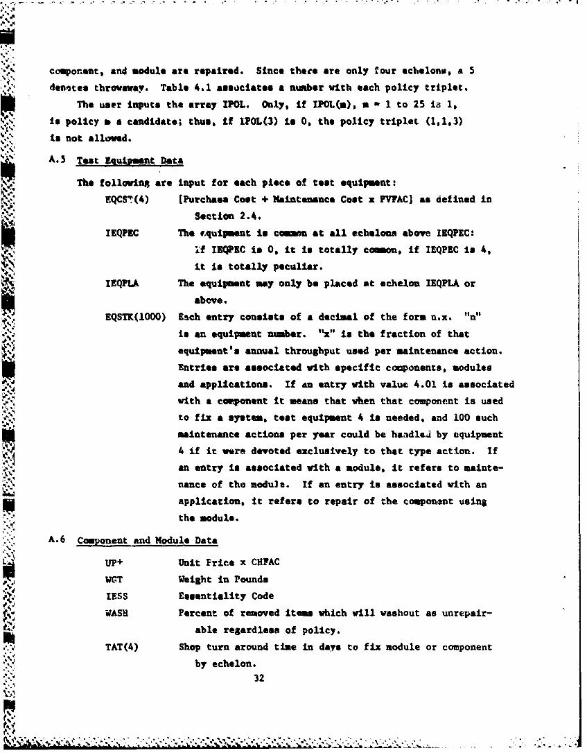
component, and module are repaired. Since thet are only four echelons, a 5

denotes throwaway. Table 4.1 associates a number with each policy triplet.

The user inputs the array IPOL. Only, If IPOL(m), a 1 1 to 25 la 1,

is policy a a candidate; thus, if IPOL(3) is 0, the policy triplet (1,1,3)

is not allowed.

A 5 Test Equiymnt Data

The following are input for each piece of test equipment:

EQCST(4) [Purchase Cost + Maintenance Cost x PVPACI as defined inSection 2.4.

IEQPBC The cquipment is coam at all echelons above IEQPEC:

if IEQPIC is 0, It Is totally comu, if IEQPEC is 4,

it is totally peculiar.

IEQPLA The equipent may only be placed at echelon IEQPLA or

above.

EQSTK(1000) Each entry consists of a decimal of the form n.x. "n"

is an equipment number. '" is the fraction of that

equipment's annual throughput used per maintenance action.

Entries are associated with specific components, modules

and applications. If an entry with value 4.01 is associated

with a comnent it means that when that component is used

to fix a system, test equipment 4 Is needed, and 100 such

maintenance actions per year could be handl&J by equipment4 if it were devoted exclusively to that type action. Ifan entry is associated with a module, it refers to mainte-

nance of the module. If an entry is associated with an

application, it refers to repair of the component using

the module.

A.6 Component and Module Data

UP+ Unit Price x CHFAC

WGT Weight in Pounds

IESS Essentiality Code

WASH Percent of removed items which will washout as unrepair-able regardless of policy.

TAT(4) Shop turn around time in days to fix module or component

by echelon.

32

5 *~SSI~

-~~~~~~ ~ ~ ~ ~ - .. % 1 - . - .. - . - _ -. . % ' .. W

INDSTK Last entry in 8QSTK (defined above) associated with theItem.

NSTACK Number of entries in FQSTK associated with the item.

PARTSR Number of new parts per module (0 for component)

PARTSP Average price of parts

DOC "One Tim Repair Costs," such as manual preparation(documentation) costs. (See Section 2.4.2)

REPC(I) The '"epair CoetI" (See Section 2.4.2)

NNSN If 0, item is new to system; fractional value can be usedvhen N) 1 -,

ID Alphanumeric ID

UN Repetition Number (Used when an "average" component ormodule represents a number, RN, of components ormodules not entered individually).

A. 7 Failure Mode Application Data

IDL Identification number of component to which failure modepertains. A component or module number is determinedby the order in which it is read in; e.g. the 5thcomponent.

IDS Identification number of module.

FAIL Number of failures per end item per year.

TAT(4) Shop turn around time to fix componeut if module fails.

NSTACK

INDS'rK Reference entries in EQSTK.

A.8 Inputs to SESAME SUBROUTINES of OATMEAL

A.8.1 CURPAR@

For components, the Lagrangian is used. (See Sections 3.5 and 3.6).

For modules, the price of the component on which it appears is used, or a weighted

average if the module appears on more than one component. For parts, the price

of the module is used. This is consistent with how part and module backorders

are coated out (Section 2.4.9).

A.8.2 WOFIL aud CONDEL

Wholesale stockage is computed for each item, and the expected W11OFI!.

and CONDEL which will result from this stockage are used for that item in coii-

puting retail stockage; thus WHOFIL and CONDEL vary by item and are conucsteut

with the dollar cost of wholesale stockage.

When FAIL pertains to average component or module (RN greater than 1), FAIIwould be multiplied by RN to get total failures.

33

Wholesale stockage is based on a reorder quantity of 1. The reorder

point is based on a target stock availability computed as:

(.60 + CIa

This is an average of .60 and the availability target appropriate at user level.

It to consistent with the findings on opttuw upper echelon availability tar.gets

documented in [3].

A.8.3 TATs and Retroarade

The user Inputs shop repair tines. Turn around times input to SISAME

include retrograde times. It is assumed retrograde times between the echelons

equal order and ship times between those echelons. It is also assumed the lower

the echelon at which a repairable is removed, the lower the echelon at which

it Is repaired.

Exsmvle:ORG DSU GSU WASHOUT

RTD 602 40%

MTD 402 302 30Z

Assumptioa:

All ORG removals are fixed at DSU (40% of 60Z) and GSU (202 of 602).

DSU removals are fixed at GSU (102 of 402) and are vashed out

(302 of 402).

Finally, in a non-vertical system, where the GSU is repairing items

for the DSU stock account, turn around time will include the time to get the good

ite from GSU to DSU.

The sarme assumptions, in fact the same computer subroutine, used to

get retrograde times are also used to get retrograde costs. Instead of time being

assessed for each retrograded item (and added to repair time), a cost is assessed

based on the retrograde cost rate.

A.8.4 Replacement Task Distribution and Maintenance Task Distributions(RTD, MT )

An RTD is a percentage breakout of the replacements of a component

or module by echelon; similarly an MT is a percentage breakout of repair of a

SV

component or module by echelon, including the throwaway/washout percentreferenced by echelon "5". It is part of the EVALUATORts job to build the

RTD L . }TDI of a component i and the RTD 1, MTD of a module j from the policy

variable values Y of the failure modes that pertain to component I or module J.ijRemeber that,

Y (PRr) - percent of failures of module j in component I for which

policy is to replace I at level P, repair I by replacing j at level F and repairjat level r. !Using these values and the proportion of failures of component i

due to module j and the proportion of module j failures that occur in component i,

one can build up the percentages, by echelon, of replace and repair associated

with P, R and r type decisions for component i and module J. Note that in thisprocedure one must adjust the module RTD's and MTD's for instances when the ext"higher assembly component was thrown out.

The aggregation or buildup of task distributions is done by surmationsover the proper indices. For example, the RTD for component i at echelon k is

found by a sumation process over J,R,r of instances involving index i, and 11 - k.

A.9 Promotion of Modules.

If the component is repaired at the same echelon as the end item and if

there is 100% repair (no washout), it is assumed the component will r.ct bestocked; instead it will be repaired so that the same component remains in t e

end item. This situation has the following ramifications:

a. Repair time for the component directly degrades operational

availability.

b. Backorders of a module used to repair the component lengthen com-"

ponent repair time and so degrade operational availability. The module is"promoted," and must be treated as an LRU.

In the MIP Formulator, when an estimate of CURPAR is derived, the possibility4 )f module promotion is not considered. Otherwise, all ramifications Of rodt,1.,

promotion are implemented.

35

4' t *'I,*S'~ 2 S',~~'t - S

4- .---. -- . - - .- .

APPENDIX B

PROPERTIES OF LAGRANGIAN AND MAINTENANCE POLICIES

Relation of Supply Lagrangian to Maintenance Policy

Figure 4 depicts a family of availability vs cost curves. The horizontal

axis consists of maintenance, transportation, supply costs - i.e., all those

costs in the ORLA model, excluding backorder penalty costs, that would be affected

by a particular maintenance posture - and the vertical axis Leesenk;s the avail-

ability achieved as the Lagrangian penalty cost (SESAME curve parameter CURPAR)

is varied and stockage costs increased. Each single curve represents one main-

tenance policy vector - a designation for every LRU and module in the system of

where to replace and repair components. The number of combinations of designa-

tions could be enormous and the figure depicts this with a partial representation

of closely spaced curve spectra. As one moves rightward, the curves represent

increased use of fix forward (more parts fixed at lower echelon); repairing at

ORG and DSU incurs relatively higher costs even for low availability (more TE,

personnel, stockage quantities) but the potential for quick repair response

allows higher availabilities to be attainable. Conversely, for curves beginning

at the lefthand portion (more and more parts maintained and stocked at higher

echelons - GSU, DEPOT) fixed zosts are generally lower but availability can be

increased (by stocking) only so much due to inherent transport delays of end items

or unserviceable assemblies rearward.

The spectral properties of the curves would not be as pure as shown

(for clarity); there would be crossing of curves due to transportation and

maintenance cost tradeoffs. The figure can be considered a response surface

on which one moves to find the best solution - achieving a target system avail-

ability while minimizing the total of all costs. The tools for conducting the

'N search are a Lagrangian (tied to a multi-echelon stockage optimizer) to vary

stockage quantities and availabilities, and a MIP to find the maintenance policy

vector that minimizes costs, including the Lagrangian tied backorder cost. In

other words, so that availability is considered in selecting policies, user level

component backorders, and delays caused by repair of the end item above user level,

are costed out using the Lagrangian and included in logistics costs.

In the discussion that follows, for consistency in the schematic exeumplifica-tion, its's indicated that the MIP chooses the leftmost curve point for a givenLagrangian value - i.e. that which has minimum cost, excluding backorder costs.

36

,~N-.... •. ,,. . ... . ....];, ujf-" .N -.. °...".... . -" , •

1-40'

'--4

A.A

0OITI.HIUE4(xldir ,c!od~ ot

03

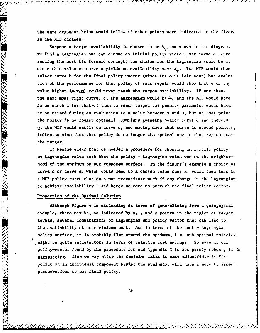
The same argument below would follow if other points were indicated on the figure

as the MIP choices.

Suppose a target availability is chosen to be AT, as shown in tue diagram.

To find a Lagrangian one can choose an initial policy vector, say curve a Lpre-

* senting the most fix forward concept; the choice for the Lagrangian would be o,

since this value on curve a yields an availability near AT. The MIP would then

select curve b for the final policy vector (since its o is left most) but evalua-

tion of the performance for that policy of rear repair would show that o or any

value higher (Ax,o) could never reach the target availability. If one chose

the next most right curve, c, the Lagrangian would be A, and the MIP would home

in on curve d for that, ; then to reach target the penalty parameter would have

to be raised during an evaluation to a value between x and c, but at that point

the policy is no longer optimal! Similary guessing policy curve d and thereby

3, the MIP would settle on curve c, and moving down that curve to around point-.,

indicates also that that policy is no longer the optimal one in that region near

the target.

It became clear that we needed a procedure for choosing an initial policy

or Lagrangian value such that the policy - Lagrangian value was in the neighbor-

hood of the optimum on our response surface. In the figure's example a choice of

curve d or curve e, which would lead to a chosen value near x, would then lead to

a MIP policy curve that does not necessitate much if any change in the Lagrangian

to achieve availability - and hence no need to perturb the final policy vector.

Properties of the Optimal Solution

Although Figure 4 is misleading in terms of generalizing from a pedagogical

Kexample, there may be, as indicated by x, , and o points in the region of targetlevels, several combinations of Lagrangian and policy vector that can lead to

the availability at near minimum cost. Arid in terms of the cost - Lagrangian

policy surface, it is probably flat around the optimum, i.e. sub-optimal policiets

might be quite satisfactory in terms of relative cost savings. So even if our

policy-vector found by the procedure 3.6 and Appendix C is not purely robust, it is

satisficing. Also we may allow the decision maker to make adjustments to th

policy on an individual component basis; the evaluator will have a mode to assess

perturbations to our final policy.

38

APPENDIX C

TEST EXPERIENCE WITH THE ,t SEARCH

Three real world end items were investigated, an expensive tactical radio

with counter-jamming features, a simple radar and a more complex radar. Table

C.1 characterizes these end items in terms of number of components, modules,

failure modes, and test equipment@.

We were interested in how well the heuristic X selection described in

Sectiona 3,6 would work. Our criteria was the cost of the solution found as

compaxed to a solution found by looping, also described in Section 3.6. While

doing this work we eviountered *n unexpected problem with the HIP procedure it-

self.

A MIP procedure has two objectives - finding an optimum solution, and

guaranteeing that the solution found is truly optimum. To save running time,any solution which is guaranteed to be within some pecent or dollar value of

the best possible solution is usually accepted am optimum. We used a criteria

of 0.5%, but also set a maxim on the amount of computer resources a KIP run

was allowed to use, about $45.

In the second iteration of the loop procedure for the tactical radio, the

MIP could not come up with a guaranteed optimum in the allotted time - in fact

all it could guarantee was that the solution found was within 6.67% of optimum.

After more than double our normal resource maximum was expended, and the MIP had

gone through 306 iterations, no better solution was found. All we learned was

that the solution already found was guaranteed to be within 6.48% rather tha-

6.67% of optimum. An additional MIP run, witn a different APEX option (different

search procedure) dId find a solution which reduced the MIP objective function

by 0.7%. In addition to the work reported here, the radio had been previously

run a number of times as the MIP FOMJLATOR program evolved, without difficulty.

A user reports no problems encountered in the analysis of a successor to the

tactical radio, albeit one with fewer pieces of test equipment.

The comparison cf heuristic and looping solutions are found in Table C.2.

Because of the problem with the radio, results were obtained for the radio with

an operational availability (OA) target of 95%, a well as for the target of 90%;

the additional target gave us another test case to investigate. Only in the case

of the complex radar did the looping solution improve on the heuristic, and

then only in terms of marginal improvement in availability per dollar.

We would acknowledge that these results may be less a tribute to the power

39

of the heuristic than to insensitivity of the maintenance policies chosen to the Xused. The X of $0.01 for the simple radar is not as aberrant as it may seem, since

field stockage rules, reflected in the SESAME stockage routines, dictate that

certain levels of stockage be calculated regardless of how low X is.

One other surprising aspect of the results was that in the loop for the

complex radar, the X values kept increasing. Intuitively, we had expected that as

we increased the A upon which the MIP inputs were based, the MIP would choose

maintenance policies resulting in fewer backorders, so that the X required in

the EVALUATOR to achieve the OA target would decrease. Under the correct assump-

tions, this intuition can be buttressed by Lagrangian theory.

Here is what caused the anomaly for the complex radar. One component had a

maintenance policy change during the looping process. At the lowest X, maintenance

policy (A) projected more component backorders, but was cheaper (including backorder

cost) then the alternative policy (B). The evaluator raised the X in order for

policy A to achieve target availability by reducing the component backorders. At

this next higher X, the MIP chose policy B over A, since, even though policy A hadfewer component backorders, its module stockage cost was high.

Finally, the X had to be further raised in the evaluator co reduce backordersof the now chosen policy A (which, by the way, was a mixed policy; hence the pro-ration scheme in Section 3.4 was used in the MIP). At this last A (31,059,002),

a final pass thru MIP and evaluator stabilized on policy B at a cost of $9,598,000.Note that this .2Z increase in cost improved the unavailability by .6% (from .0148

to .0147).

%I,I'I

40

'a

TABLE C.1 EXAMPLE CHARACTERISTICS

NUMBER OF

FAILURE TESTEXAMPLE COMPONENTS MODULES MODES EQUIPMENTS

TACTICAL RADIO 19 61 61 15

SIMPLE RADAR 3 16 16 1

COMPLEX RADAR 11 37 37 5

4'.'

41

I * ' 4. '" %Z , . . , ' . ," ' ! : "- : ! : ' ' ' 4 "- * ! . " , . . ." ' " ' 4 ,.' l ', '' . . ' '' ' ' '

" ''

.44V

.44

ta ON co H HH0 0 0~ 0% 0 0S %

V4 0n * ** *

-~ 0 0% 0% m% 0% 0%0% 0%

000

r4 4% 51 iIi

p42

APPENDIX DCOMPUTER COSTS AND RUN TIMES

Before discussing run times and costs, we will devote a section to a

theoretical principle which avoided combinatorial problems in programming

the assessment of maintenance policies over many items.

Principle of Independence in Use of SESAME Subroutine

One principle, that contained in the SESAME optimization process, in-

herently reduces the run times in the MIP. On the surface one might think

that in any one cost evaluation step, specific maintenance policies on each

LRU would have to be considered simultaneously in order to assess cost and

perfo-mance for a specified Lagrangian value; therefore the number of com-

binations of policies over the LRUs would be enormous.

However, in the SESAME optimization process, given the Lagrangian value,

the individual item supply availabilities are "set" based on the items' unitprices relative to this value. Each Item (LRU) is optimized independently

N (multiechelon allocation of stockage quantities) to achieve its target.

An item's optimal stockage of course will be dependent on its maintenance

policy, but independent of the other Items' policies. This principle allows,

for a set Lagrangian value, a SESAME subroutine of the ORLA program to

compute the optimal s o-kage costs for an item under some pure maintenance

policy (e.g. 100% replacement at some echelon and 100% repair at some echelon)

without having to simultaneously consider hybrid combinations of policiesViNacross all item. The ORIA "optimizer" uses the results of the SESAME module

(stockage costs, backorders by item by pure policies), in conjunction with

other logistical costs, to find the best maintenance policy vector across

all items for a given Lagranpl-.

Experience With Coia ..er Cci,.e

A commercial time sharing service was used for the work reported here.

Costs reported are based on pri".rity 02 which guarantees 12 hours response time.

Actual response times are most ---an a few minutes and never exceed a few hours.

The costs reflect a substantial volume discount. They do not include an input/

output charge as we did not keep an accurate record of these. For the MIP runs,

costs include a large surcharge for use of the APEX program; this surcharge

is computed as a multiple of usage costs.

4% 43

The cost of running the KIP FORMULATOR for the radio was about $6.50. Cots

for the EVALUATOR were smaller. This was in line with expectations since the

SESAME routines which are the heart of these programs run fast.

The range of costs encountered in running NIP for the radio is shown below.

There were 97 constrai-ts and 938 variables of which 30 were integer. Of the

30 integer 17 were binary, and the largest upper bound for any integer variable

was 62. The different runs varied only in the coefficients of the objective

function. The sensitivity of run costs to changes in caefficients has been

noted by many other KIP users.

RUN COST

Heuristic- OA- 902 $38

Loop - OA 90% $42

Heuristic - OA - 95% $13

Loop - OA - 95% $13

Reduci Running Times for the .IP

The logistician often kVows a priori that certain solutions would be too

costly or would otherwise be unacceptable. He can input this knowledge in two

ways: he can specify the lowest echelon at which a piece of test equipment can

be placed, or he can rule out certain policies; e.g. no end item repair above

user level.

Preliminary analysis may be used to identify upper bounds on echelon testequipment requirements; i.e. the requirement if all repair using that equipment

were performed at that echelon. Typically, the bound will be 1, transforming

the integer into a binary variable.

This concept can be carried further with some degradation in the optimality

of the solution. For each tk associate t'e k where t'ek is continuous and!

let M be a "large" integer.

Set

to ek I (tek) x ()

I' < k e

ek EM)il

lRun stopped because limit on computer costs reached.

44

In the first came we permit continuous values for test equipment provided they

exceed 1. In the second case continuous values less than 1 are permitted

if at least 1 tet equipment per facility has been deployed at a lower echelon.

The rationale is that if we must round up to 1 at a higher echelon, we have not

miscalculated too severely since the algorithm alrody had costed out integer

quantities at a lower echelon where there are typically &my more facilittes.

Furthermore, an optimum policy would not tend to purchase test equipment at a

highi-r echelon when all requirements could be met by equipment already purchased

for the lower echelon.

Under the simplified formulation we smay add the constraint

r (1k-l

which further speeds the HIP. This is not an equality because of the possibility

of component or module discard in which case the equipment is not needed at all.

45

4'.,,, ,..'., . ,',. - ".': . . , . . : e ' ' .: ";2 '.- -.- -: - "

. . . . • -

0 ~REIERNCES

I Control Data Corporation, "APEX-Ilk Reference Manual, Version 1.k,"

Minneapolis, 1979.

2 Everett III, Hugh, "Generalized Lagrange Method for Solving Problems of

Optmum Allocation of Resources," Operations Research, Vol I:, 1963, p333-417.

3 Frauza, Sally and Alan J. Kaplan, "Supply Performance Objectives for Upper

Echelons in a Multi-Echelon Supply System," AMSAA Army Inventory Research

Office, Philadelphia, December 1981.

4 Grfinkel, Robert S. and George L. Nemhauser, "Integer Programming," John

Wiley. New York. 1972.

5 Kaplan, Alan J., "Mathematics of SESAME Models" AMSAA Army Inventory

Research Office, Philadelphia, February 1980.

6 Kaplan, Alan J., Notes, Unpublished.

7 Mitchell, Terrance and Lawrence Briskin, "Network Repair Level Analysis

Model User's Guide," Air Force Logistics Command, Wright-Patterson AFB,

June 1982.

8 Plumeri, Charles J., "Optimum Supply and Maintenance Model Users' Guide,"

CECGR, Ft. Monmouth, NJ, September 1982.

9 Seegers J. P., "B-4B Network LSA Model," MITRE, June 1980, WP22361.

10 DARCIM Pamphlet 700-18, "User's Guida for the Selected Essential-Item

Stockage for Availability Method (SESAME) Program," March 1980.

11 DARCOM Pamphlet 700-10-1, "Pro-risioning Models," Draft.

12 DoDI 7041.2, "Economic Analy1.e and Program Evaluation for Resource

Management," October 1972.

46

• , .wwv-. - - , *,** * * .--. - - - ,a.- . : r rr i r* r' rrr 1-'

DISTRIBUTION

" . co~zu

Deputy Under Sec'y of the Army, ATTN: Office of Op ReachAsst Sec y of the Army (IL&N), Pentagon, Wash., DC 20310Headquarters, US Army Materiel Development & Readiness Command

1 DRCDKRDIC24-SDRCD1M

1 DRCSM--DRCSX-E

1 DRCSN-WDRCSM-WR

1 DRCSK-RS

1 DRCSM-PDRCSHaPAS

1 DRCREDROIS

1 DRCQAI 1 DRMDKDep Chf of Staff for Logistics, Pentagon, Wash., DC 20310

1 DALO-S4P-U

U. 1 DALO-S4B"-'I'-- so.

____ DALO-AVOfc, Asat Sec'y of Defense, ATTN: RA&L-SR, Pentagon, Wash., DC 20310

2. Defense Technical Info Center, Cameron Station, Alexandria, VA 22314

Comnder, USA Arm iment Material Readiness Cod, Rock Island, IL 61299I DRSAR-M1 DRSAR-Sk

CosanderA USA Missile Cowwand, Redstone Arsenal, AL 35898

1 DRSMI-S1 DRSMI-D

Cosmander, USA Troop Support & Aviation Materiel Readiness Command,St. Louis, MO 63120

1 DRSTS-SPF1 DRSTS-SPS1 DRSTS-BA

Comander, US Army Tank-Automotive Commnd, Warren, MI 480901 DRSTA-V1 DRSTA-S

Coumander, USA Communication-Electronic' Cad, Ft. Monmouth, NJ 07703

1 DRSZL-XOIDRSEL-PL-SA

T... Comander, USA Armament R&D Cad, ATTN: DRDAR-SE, Dover, NJ 07801. Comander, USA Aviation R&D Cd, 4300 Goodfellow Blvd, St. Louis, 1O 631201 Commander, USA Aviation R&D Cad, ATTN: DRDAV-BD (Marl Glenn), 4300

Goodfellow Blvd, St. Louis, MO 631201 Comeander, USA Electronics R&D Cod, ATTN: DRDEL-PO-SA, Rn 2D315,

Bldg. 2700, Ft. Monmouth, NJ 07703

47

- -.. ,= ' ' - , ,-.. -:- , '... ,'"2'- VV -"2";".', . .. 2:..'-'.:-*,-,.. -'". ,*-..,*,'.;'?

•- r.r *- r.o, -

jComander, USA Mobility Equipment R&D Cad, ATTN: DRDME-US (Leon Medler)Ft. Delvoir, VA 22060

.J. Commander, USA Natick R&D Cud, ATTN: DRXN- O, Natick, MA 01760Director, Army aterial Systems Analysis Activity, APC, MD 21005

~DV-DDRXSY-D

. ' __j.._DawS~-C

D3XSY-FX

D3XSY-DA

T DI SY-FA

D3XSY-PM2DRZXSY-PX ATTN: Sandy Johnson

_1 Cosmander, US Army Logistics Center, Ft. Lee, VA 23801.. j Comander, US Amy Logistics Rvaluation Agency, Now Cumberland Amy

Depot. New Oberland, PA 17070-1L. Coaunder, US Army Depot Systems Command, Chambersburg, PA 17201

J Comeander, US Air Force Logistics Cod, WPAPB, ATTN: A LC/XRS, Dayton,Ohio 45433I *...j.. US Navy Fleet Materiel Support Office, Naval Support Depot, OperationsAnalysis Departmentq Code 93, Mechanicsburg, PA 17055

_ Mr. James Prichard, Navy SEA Systems Cud, ATTN: PMS 3061, Dept ofUS Navy$ Wash., DC 20362

-. George Washington University, Inst. of Manageuent Science & Engr.,707 22nd St., N.W., ash., DC 20006

Naval Fostgraduate School, ATTN: Dept of Opus Anal, Monterey, CA 93940Air Force Institute of Technology, ATTN: SLGQ Head Quantitative Studies

Dept., Dayton, OH 43433US Army Military Academy, West Point, NY 10996

1 Commander, US Army Logistics Center, ATTN: Concepts & DoctrineDirectorate, Ft. Lee, VA 23801

I Scientific Advisor, ATCL-SCA, Army Logistics Center, Ft. Lee, VA 23801_l HQ, Dept of the Army, (DASG-HCL-P), Wash., DC 20314

-___ Librarian, Logistics Mgt lust., 4701 Sangamore Rd., Wash.,DC 200161 University of Florida, ATTN: Dept of Industrial Systems Engr.,

Gainesville, FL 32601I RAND Corp., ATTN: S. M. Drener, 1700 Main St., Santa Monica, CA 904061 ALOG Magazine, ATTN: Tom Johnson, USALMC, Ft. Lee, VA 238011 Wallace M. Cohen, Anst Director Systems Analysis, FGMSD, General

Accounting Ofc, Wash., DC 20548Comander, USDRC Automated Logistics Mgt Systems Activity, P.O. Box 1578,

St. Louis, MO 63188Director, DARCON Logistics Systems Support Agency, Lette-kenny

Army Depot, Chambereburg, PA 17201

1 Comander, Materiel Readiness Support Activity, Lexington, KY 40507Director, Army Management Engineering Training Agency, Rock Island

Arsenal, Rock Island, IL 61299S- Defense Logistics Agcy, ATTN: DLA-LO, Cameron Sta, Alexandria, VA 22314

48

a,, ,f , -. '.,, -... . .. -,,. ,..... ..-........... . .. ,'1

Dep Chf of Staff (I&L), HQ USMC-LMP-2, ATTN: LTC Sonneborn, Jr.,Wash., DC 20380

Comander, US Army Depot Systeas Ccuand, Letterkenny Army Depot,ATTN: DRSDS-LL, Chambersburg, PA 17201

1 Logistics Control Activity, Presidio of San Francisco, CA 94120Operations Research Canter, 3115 Etcheverry Hall, University of

California, Berkeley, CA 947201 Dr. Jack Muckstadt, Dept of Industrial Engineering & Operations Research,

De Upson Hall. Cornell University, Ithacao NY 1 A890Dept of Industrial Enineive, rsity of Michigan. Ann Arbor

MI 48104

Prof Robert M. Stark, Dept of Stat & Computer Sciences,University of Delaware, Newark, DR 19711

Prof E. Gerald Hursts Jr.$ Dept of Decision Science, The WhartonSchool, University of Penna., Phila., PA 19104

1 Director, AMSAA, ATTN: Allen Hill, DRXSY-FLSO, Ft. Lee, VA 238011 Director, AMSAA, ATTN: Paul Arvis, DAXSY-PRO, Ft. Lee, VA 23801

Dept of Industrial Engr. 4 Engr. Managment, Stanford University,Stanford, C 94305

1 Comander, US Army Commnications Connd, ATTN: Dr. Forry,CC-LOG-LEO, Ft. Huachuca, AZ 85613

. Commander, US Army Test & Evaluation Cad, ATTN: DRSTE-SY,Aberdeen Proving GroundsMD 21005

1 Prof Harvey M. Wagner, Dean, School of Business Adm, Universityof North Carolina, Chapel Hill, NC 27514

Pentagon Library, ATTN: ANR-AL-RS (Army Studies), Pentagon, Rm 1A518,Wash., DC 20310DARCOM Intern Training Center, Red Rivet Army Depot, Texarkana, .

Dx 75501Prof Leroy B. Schvars, Dept of Management, Purdue University,

Krannert Bldg, West Lafayette, Indiana 47907I US Army Training & Doctrine Commnd, Ft. Monroe, VA 23651T US General Accounting Office, ATTN: Mr. J. Morris, Rm 5840,

441 G. St., N.W., Wash., DC 205481 Operations & Inventory Analysis Office, NAVSUP (Code 04A) Dept

of Navy, Wash., DC 20376US Amy Research Office, ATTN: Robert Launer, Math. Div.,

P.O. Box 12211, Research Triangle Park, NC 277091 Prof William P. Pierskalla, 3641 Locust Walk CE, Phila., PA 19104

Air Force Logistics Mgt Center, Gunter A.r Force Station, AL 361441AFLMC/LGY

AFLMC/XP, Bldg. 205Engineer Studies Center, 6500 Brooks Lave, Wash., DC 20315Dr. Carl Weisman, C.A.C.I., 1815 N. Fort Myer Drive, Arlington, VA 22209Commander, US Army Missile Cmd, ATTN: Ray Dotson, DRSMI-DS, RedstoneArsenal, AL. 35898

1 Prof Peter Kubat, Graduate School of Mgmt, University of Rochester,Rochester, NY 14627

1 Prof Barney Bissinger, The Pennsylvania State University, Middletow.n,

PA 17057Prof Garry D. Scudder, Mgmt Sciences Dept, College of Business Adm,

University of Minnesota, 271 19th Ave., South, Minneapolis, MN 55455

49

w '.S

1 Center for Naval Analyses, ATTN: Stan Horowitz, 2000 N. BeauregardSt., I4lexandria, VA 22311

1 Dr. Warren H. Hausman, Industrial Engr. & Engr. Management, StanfordUniversity, Stanford, CA 94305

1 Dr. Paul Zipkin, Graduate School of Business, Columbia University,416 Uris Hall, New York, NY 10027

_i_ Mr. Craig Sherbrooke, Logistics Management Institute, 4701 S&:ngamoreMr.JRoad, Wash., DC 20016 on

_1 Mr. Charles Groover, Deputy Asst Sec'y of Defense (Requirements Resources& Analys:is), Room 3E784, Pentagon, Wash., DC 20310

Dr. Richard D. Webster, Deputy Asst Sec'y of Defense (Supply Maintenance& Transportation), Room 3E760, Pentagon, Wash., DC 2031f

1 Mr. Eric Orsini, Deputy for Logistics, Asst Sec'y of the Army ,LL.&FM),Room 3E620, Pentagon, Wash., DC 20310

1 Comnander, CECOM, ATTN: Charles Plumeri, DRSEL-PL-E, Ft. Monmouth,NJ1_ Commander, CECOM, ATT14: Mike O'Donnell, DRSEL-FMD-RD-C, Ft. Monmouth,

NJ 077031 Mr. Mike McGrath, Office Asst Sec'y of Defense, Manpower, Reseserve

Affairs & Logistics, Pentagon, Wash., DC 203101 Commander, US ArmyM issile Cmd, ATTN: Tom Prestwood, DRSMI-SL,

Redstone Arseeil, AL 358981 RAND Corp., ATTN: .Mr. Jack Abell, 1700 Main St., Santa Monica, CA 904061 RAND Corp., ATTN: Mr. Milt Kamins, 1700 Main St.,Santa Monica, CA 90406

J

44.

5 0

05