Embed Size (px)
Citation preview

Inventory Positioning, Scheduling and Due-Date Quotation in
Supply Chains
Philip Kaminsky
Onur Kaya
November 2006
Abstract
We consider supply chain networks composed of several centrally managed production facilities as
well as external suppliers. We design effective heuristics for inventory positioning, order sequencing, and
short and reliable due date quotation for this supply chain. We perform extensive computational testing
to assess the effectiveness of our algorithms, and we explore the impact of supply chain topology on
inventory costs and effective due date quotation.
1 Introduction
Inventory costs make up a large portion of total costs in many supply chain, so effective inventory manage-
ment is one of the most important issues facing many supply chain managers. Indeed, in a multi-facility
supply chain, a critical tactical decision involves the identification of stocking points in the supply chain,
and the determination of appropriate inventory strategies at these stocking points. In other words, facilities
that will produce to stock and thus keep inventory and the amount of that inventory, and facilities that will
produce to order and hence keep no inventory, must be identified. In this paper, we develop an approach to
address this typically quite difficult problem.
There is increasing pressure on supply chains in many industries to reduce costs and to improve service
levels to remain competitive. Traditionally, most companies utilized a ”push” system (i.e Make-to-Stock
(MTS) system), holding inventory at the end of the supply chain. However, in a MTS system, firms need
to be able to estimate demand to determine how much to produce and stuck, and thus these systems rely
heavily on forecasts. Unfortunately, forecasts are typically not very accurate. In addition in push systems,
1

order variance typically increases up the supply chain, in a phenomenon known as the ”bullwhip effect”.
Lee et al. [16] show that information transferred in the form of orders tends to be distorted and leads to
errant inventory and production decisions. This increase in variability leads to excessive inventory due to
the need for large safety stock, large and more variable production batches, unacceptable service levels, and
the inability to manage resources effectively. In general, push systems make it difficult for firms to react
quickly and effectively to changes in the marketplace, and thus typically lead to high inventory costs and
decreased profits.
Thus, many progressive companies have shifted to ”pull” systems (i.e make-to-Order (MTO) systems),
holding no inventory at all and producing to order. In these systems, companies produce based on actual
customer demand instead of forecasts. Inventories are eliminated, there is no bullwhip effect, service levels
increase, and companies can react better to changes in the market. However, these systems also has their own
set of problems. For example, delivery lead times can be quite long, and implementation difficulties arise in
many industries. Long production and delivery lead times can lead to loss of competitiveness and ultimately
decreased sales. Furthermore, it is difficult to take full advantage of economies of scale in production and
distribution in pull systems.
The decision to use either a push strategy or a pull strategy in a facility therefore depends heavily on the
characteristics of the system. In a supply chain, using a push strategy at some facilities and a pull strategy
at others might be much more effective then using either system exclusively. Because of this, firms are
beginning to employ a hybrid approach, a ”push-pull” strategy (i.e. Combined MTO-MTS system), holding
inventory at some of the facilities in their supply chain and producing to order in others.
Push systems can be better utilized if long-term forecasts have small uncertainty and variability and can
be reasonably predicted, whereas pull systems might be more beneficial if uncertainty and variability are
high. Typically, the initial stages of a supply chain employ a push system and later stages utilize a pull
system. In this paper, we consider a general supply chain and depending on the properties of the system
and products, we determine which facilities should produce to order and which should produce to stock,
and stocking levels at the produce-to-stock facilities. In our approach, we focus on globally optimizing the
system rather than employing the traditional approach in which each stage is locally optimized.
There is a vast amount of literature on inventory placement models for multi-stage systems applicable to
supply chains. Axsater [1], Federgruen [5], Inderfurth [12] and Diks et al. [3] survey these models in detail.
Several researchers including Inderfurth [10, 11], Inderfurth and Minner [13] and Minner [22] analyzed the
problem of optimizing safety stock placement in supply chains based on the framework of Simpson [23], who
analyzed a serial supply chain to determine the optimal safety stock placement and found that the optimal
2

solution is an ”all or nothing” strategy for that model. A dynamic programming approach is typically used in
this analysis. Graves and Willems [7, 8, 9] extended the results of Simpson [23] to assembly, distribution and
spanning tree network structures. In addition, Lee and Billington [15], Glasserman and Tayur [6] and Ettl
et al. [4] examine the determination of optimal base-stock levels in a supply chain and develop algorithms to
optimize the safety stock placement in their models. Magnanti et al. [21] models the problem of inventory
placement in supply chains as a nonlinear program and uses successive piecewise linear approximation to
obtain a tight approximation for the problem.
In addition to inventory decisions, scheduling of the production of orders and lead time quotation to
customers also has significant impact on the performance of the supply chain, particularly MTO supply
chains. Companies need to quote short and reliable lead times to their customers to remain competitive
in the market and to increase their profits. For a company that produces multiple products with different
characteristics, the decision on when to produce each order affects the completion time of manufacturing
and thus the lead time for that product. In spite of this, most research on inventory positioning in supply
chains ignores the intricacies of scheduling and lead time quotation, typically assuming that lead times are
exogenously determined, and that orders are processed in sequence if which they arrive at the system.
In contrast to the research discussed above, we focus on integrating scheduling and lead time quotation
into the determination of optimal safety stock placement in supply chains. We develop algorithms for
addressing these issues, and computationally test these inventory, scheduling and lead time quotation (LTQ)
algorithms. We also consider multiple products and congestion effects in the system and computationally
analyze how strategic safety stock placement will affect the system costs. In addition, we consider different
supply chain structures and analyze the effect of supply chain structure on effective inventory placement,
scheduling and lead time quotation, in order to extract managerial insights from these models.
In Kaminsky and Kaya [18], we analyze pure MTO supply chains and design effective scheduling and
due-date quotation algorithms for the centralized and decentralized versions of those systems. We show
that these algorithms are asymptotically optimal(i.e. optimal as the number of orders n → ∞) for the
minimization of a function of lead time related costs and tardiness related costs (or more specifically, for the
function Zn =∑n
i=1 (cddi + cT Ti) where di is the quoted due-date for job i, Ti = (Ci − di)+ is the tardiness
of job i and cd and cT are the unit due date and tardiness costs for the model).
In Kaminsky and Kaya [19], we integrate inventory decisions, scheduling and due date quotation issues for
combined MTO-MTS systems for a two-facility supply chain. We develop models that provide guidance in
deciding when to employ MTS and when to use MTO approaches, and how to effectively operate the system
to minimize system-wide costs. We also quantify the value of centralization and information in these systems
3

by building decentralized and centralized models, obtaining good solutions to these models, and designing
computational experiments to explore the effectiveness of our algorithms and to compare the centralized and
decentralized systems.
In this paper, we utilize many of the results in Kaminsky and Kaya [18, 19], and extend our approach to
multi-facility systems under a variety of conditions. We design effective algorithms for scheduling, lead time
quotation and inventory decisions to minimize total costs for these systems. We explain our model in detail
in the next section and then, in Section 3, we propose a solution approach for this model and present our
algorithms. In Section 4, we present the computational results from using these algorithms and analyze and
compare different supply chain structures under different conditions to assess the effects of the parameters
on our decisions and on supply chain performance.
2 Model
We consider a manufacturing firm facing stationary stochastic demand, whose supply chain consists of a
single downstream stage (which we call the manufacturer) that receives orders from customers, and a series
of stages upstream from this manufacturer, which we call the internal and external suppliers (depending on
whether or not the managing firm controls these stages), where other manufacturing steps may take place.
The manufacturer receives customer orders over time, fills these orders immediately if the product ordered
is in inventory at the manufacturer, and quotes lead times for these orders if they are for items that are not
in inventory at the manufacturer. There are a total of N facilities in the supply chain, and K product types
offered by this firm to its customers. We assume a stationary demand process for the demand that arrives
at the manufacturer, with known and possibly different arrival rates for orders for each of the products. In
particular, orders arrive at rate D and each arriving order is for job type i with probability δi, i = 1, 2, ...K.
To facilitate our analysis, we assume stationary and independent inter-arrival times, so each order for job
type i arrives at rate Di = Dδi. Each product must be processed at a specified subset of the facilities in the
supply chain, in a specified order, with specified processing times. Each product type thus has a predefined
routing through the supply chain. We assume a known deterministic production time pij for an order type i
at facility j (if that product is processed at that facility, of course) and a known deterministic transshipment
time tijk to move a product type i from facility j to k.
Typically, firms prefer to quote short lead times for products. If processing times for a particular product
are short and the production network is relatively uncongested, then the firm doesn’t need to hold inventory,
and can instead use an MTO approach and achieve the desired short lead time with minimal inventory.
However, the total required processing time to manufacture a product is frequently greater than the desired
4

Customer
Figure 1: Supply Chain Structure
lead time, and since demand is stochastic, firms must start manufacturing products before specific orders
for these products actually arrive, and thus must keep some inventory in order to not exceed their desired
maximum lead time. Clearly, keeping finished goods inventory at the manufacturer is not the only available
option for reducing lead times. Instead, firms may have the option to store intermediate inventory at some
of the other facilities (i.e. some of the suppliers) in order to reduce lead time. Our goal in this paper is to
present an effective approach for (1) determining locations at which to store inventory in this supply chain,
(2) sequencing specific jobs at specific facilities, and (3) quoting lead times, so that system-wide costs are
minimized, quoted lead times are relatively short, and these quoted lead times are typically met.
We consider a supply chain network with nodes representing facilities in the production network at
which specific operations (manufacturing, assembly, etc.) take place, and with arcs representing the flow
of components. This network is thus represented by a directed and acyclic graph G, and we assume that
each product type i has a known production network which is a subgraph of the entire supply network. In
particular, the production operations/locations of each order of type i can be represented by a subgraph Gi
composed of a specified subset of the nodes and arcs in graph G. For ease of exposition, we assume that
only one unit of upstream component i is required per downstream unit j. As mentioned above, we assume
that a single firm owns the downstream manufacturer and the internal suppliers over whom it has complete
control, but there also may be external independent suppliers over whom the manufacturer has no control.
An example is presented in Figure 1, where the internal supplier nodes are represented with rectangles, and
the external supplier nodes are represented with circles.
In our model, we assume that each facility observes demand from its downstream stage and places orders
to its suppliers to replenish the observed demand. There is no time delay in ordering, thus, when a customer
5

order arrives at the manufacturer, the external demand is passed back up the supply chain and every facility
sees the external demand immediately.
As we discussed above, since the demand is stochastic, we need to carry some inventory to respond
rapidly to customer orders. Each stage in the network is a potential location for holding inventory of the
item processed at that stage, and we can choose to stock intermediate inventory in this system instead
of choosing to stock only finished goods at the downstream facility. We assume that each stage in our
model operates with an order-up-to inventory policy and every time an order arrives, each facility starts the
production of that type immediately, either to satisfy that order or to replenish inventory if that order is
satisfied from the existing inventory.
We assume that for each product type i and its associated production network, for the production of
that product or one of its associated components at facility j, an inventory (or safety stock) of components
required from some other facility k, that will last on average xikj units of time (with associated unit holding
cost h1ikj) and an inventory (or safety stock) of finished products of facility j, that will last on average yij
units of time (at a unit holding cost of h2ij) is held at facility j. In our model, products might share common
components that is, a component produced by a facility might be required for the production of two or more
products.
Note that, throughout this paper, we denote all the inventory amounts in terms of the time length (e.g.
days, hours, etc.) that the inventory will last. We can find the exact amount of inventory using this time
length, the specified service level that we operate with, and the demand distribution. For example, if we
denote the amount of inventory as 4 days worth of inventory, then at a 95% service level where the demand
is normally distributed with mean 2 and variance 1 per day, the actual amount of inventory that we need to
stock is equal to 2 ∗ 4+√
4 ∗ z0.95 = 11.92. Also note that holding cost is assumed to be in appropriate units
for this notation, and these inventory levels can be zero if the product is purely made-to-order at that stage.
Our goal is to quote short and reliable lead times without holding excessive inventory in the system.
Thus, we attempt to minimize the following objective function:
K∑
i=1
{(N∑
j=1
hijE[Iij ]) + cdi E[di] + cT
i E[Wi − di]+} (2.1)
consisting of inventory costs, lead time costs, and tardiness costs. In particular, E[Iij ], E[di] and E[Wi−di]+
denote the average inventory level at facility j, the average quoted lead time, and the average tardiness for
product type i. For each product type i, the average cost of inventory at facility j, hijE[Iij ] represents both
components and finished goods inventory such that hijE[Iij ] = h2ijyij +
∑k∈Pij
h1ikjxikj where Pij denotes
the set of facilities that are predecessors of facility j in the production network of product type i. Also, cdi
6
and cTi denote the unit lead time cost and the unit tardiness cost for product type i.
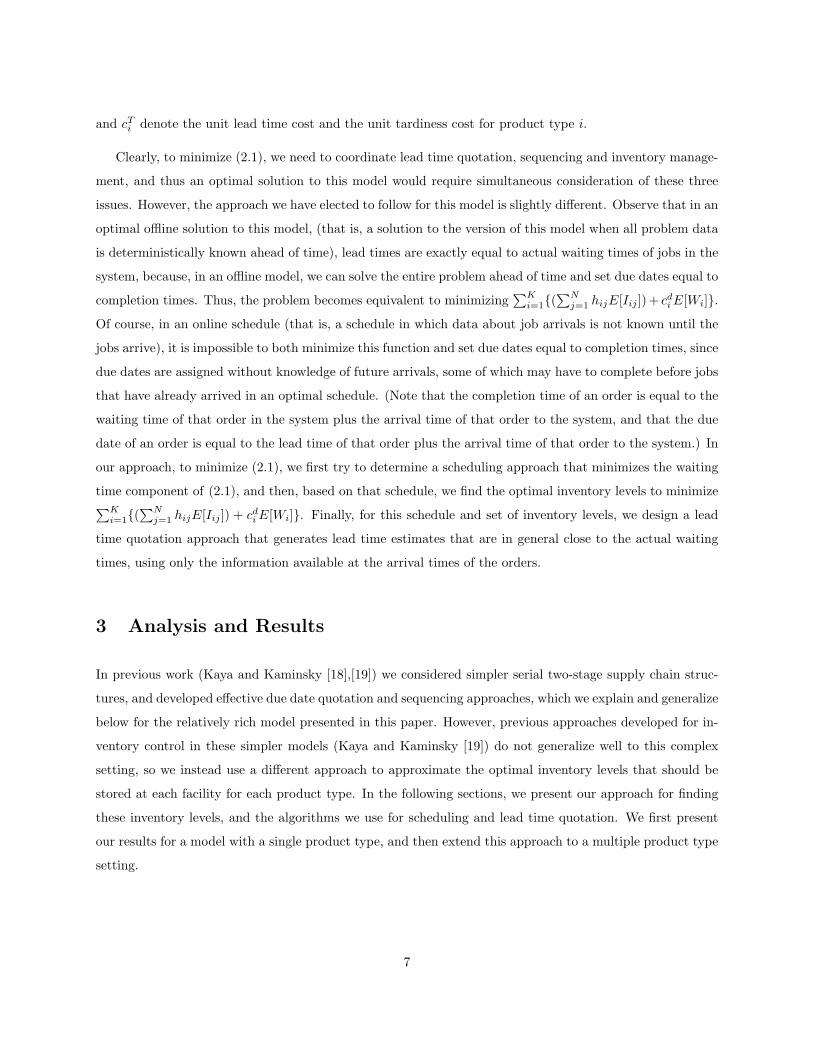
Clearly, to minimize (2.1), we need to coordinate lead time quotation, sequencing and inventory manage-
ment, and thus an optimal solution to this model would require simultaneous consideration of these three
issues. However, the approach we have elected to follow for this model is slightly different. Observe that in an
optimal offline solution to this model, (that is, a solution to the version of this model when all problem data
is deterministically known ahead of time), lead times are exactly equal to actual waiting times of jobs in the
system, because, in an offline model, we can solve the entire problem ahead of time and set due dates equal to
completion times. Thus, the problem becomes equivalent to minimizing∑K
i=1{(∑N
j=1 hijE[Iij ])+ cdi E[Wi]}.
Of course, in an online schedule (that is, a schedule in which data about job arrivals is not known until the
jobs arrive), it is impossible to both minimize this function and set due dates equal to completion times, since
due dates are assigned without knowledge of future arrivals, some of which may have to complete before jobs
that have already arrived in an optimal schedule. (Note that the completion time of an order is equal to the
waiting time of that order in the system plus the arrival time of that order to the system, and that the due
date of an order is equal to the lead time of that order plus the arrival time of that order to the system.) In
our approach, to minimize (2.1), we first try to determine a scheduling approach that minimizes the waiting
time component of (2.1), and then, based on that schedule, we find the optimal inventory levels to minimize∑K
i=1{(∑N
j=1 hijE[Iij ]) + cdi E[Wi]}. Finally, for this schedule and set of inventory levels, we design a lead
time quotation approach that generates lead time estimates that are in general close to the actual waiting
times, using only the information available at the arrival times of the orders.
3 Analysis and Results
In previous work (Kaya and Kaminsky [18],[19]) we considered simpler serial two-stage supply chain struc-
tures, and developed effective due date quotation and sequencing approaches, which we explain and generalize
below for the relatively rich model presented in this paper. However, previous approaches developed for in-
ventory control in these simpler models (Kaya and Kaminsky [19]) do not generalize well to this complex
setting, so we instead use a different approach to approximate the optimal inventory levels that should be
stored at each facility for each product type. In the following sections, we present our approach for finding
these inventory levels, and the algorithms we use for scheduling and lead time quotation. We first present
our results for a model with a single product type, and then extend this approach to a multiple product type
setting.
7

3.1 Single Product Type Model
In this section, we assume that the firm produces only one type of product. For more than one product, to
minimize the objective function (2.1), we first attempt to sequence the jobs in order to minimize the total
waiting times of the products. However, since there is only one type of product in this case, we use the
commonly used scheduling approach FCFS (First Come First Served) to sequence the jobs at all facilities.
In most of the literature for inventory placement in supply chains, researchers assume deterministic lead
time for the production of components at all the facilities to make the analysis of the system easier (e.g.
Magnanti et al. [21], Graves and Willems [8] etc.). To approximate the optimal inventory levels, for now, we
also make the same assumption. That is, we assume that processing times are deterministic and each server
has no capacity restriction, so that any number of jobs can be processed simultaneously at any facility in the
system. Thus, although the demand is stochastic, the orders don’t effect each other and the waiting time
of the jobs at all the facilities are deterministic and known in advance. Later, we will relax this assumption
and generalize our results to facilities with capacity restrictions at each facility.
For an uncapacitated single stage system, the lead times, inventory values and processing times satisfy
the relation l = max{p − x, 0} where p is the deterministic processing time required to process an order, l
is the lead time and x is the length of time that the available safety stock lasts. Since the production lead
time is p and the demand can be satisfied from the inventory for x time units, the first order that arrives
after the inventory is depleted at time x, can only be satisfied at time p, leading to a lead time l = p − x
assuming p > x. If p < x, then l = 0 since, in this case, we can satisfy all the demand from the inventory
and replenish the inventory before it is depleted.
Using this relationship, we write a linear program to approximate the optimal inventory levels at each
facility. The objective function to be minimized is composed of the total inventory plus the lead time costs
and the constraints ensure that the lead time for the production of a component at a facility is no less than
the lead time required for the components to arrive at that facility plus the required processing time minus
the safety stock values. We define the parameters and variables and write the LP formulation of this model
below:
Parameters:
j, k = subscripts used to describe the facilities in the supply chain starting with j = 1 denoting the
manufacturer.
pj = processing time at facility j
tkj = transshipment time to move from facility k to j
8
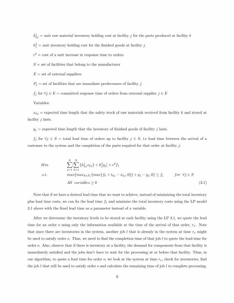
h1kj = unit raw material inventory holding cost at facility j for the parts produced at facility k
h2j = unit inventory holding cost for the finished goods at facility j.
cd = cost of a unit increase in response time to orders.
S = set of facilities that belong to the manufacturer
E = set of external suppliers
Pj = set of facilities that are immediate predecessors of facility j
fj for ∀j ∈ E = committed response time of orders from external supplier j ∈ E
Variables:
xkj = expected time length that the safety stock of raw materials received from facility k and stored at
facility j lasts.
yj = expected time length that the inventory of finished goods of facility j lasts.
fj for ∀j ∈ S = total lead time of orders up to facility j ∈ S, i.e lead time between the arrival of a
customer to the system and the completion of the parts required for that order at facility j.
Min
N∑
j=1
[N∑
k=1
{h1kjxkj}+ h2
jyj ] + cdf1
s.t. max{maxk∈Pj{max{fk + tkj − xkj , 0}}+ pj − yj , 0} ≤ fj for ∀j ∈ S
All variables ≥ 0 (3.1)
Note that if we have a desired lead time that we want to achieve, instead of minimizing the total inventory
plus lead time costs, we can fix the lead time f1 and minimize the total inventory costs using the LP model
3.1 above with the fixed lead time as a parameter instead of a variable.
After we determine the inventory levels to be stored at each facility using the LP 3.1, we quote the lead
time for an order o using only the information available at the time of the arrival of that order, ro. Note
that since there are inventories in the system, another job l that is already in the system at time ro might
be used to satisfy order o. Thus, we need to find the completion time of that job l to quote the lead-time for
order o. Also, observe that if there is inventory at a facility, the demand for components from that facility is
immediately satisfied and the jobs don’t have to wait for the processing at or before that facility. Thus, in
our algorithm, to quote a lead time for order o, we look at the system at time ro, check for inventories, find
the job l that will be used to satisfy order o and calculate the remaining time of job l to complete processing.
9

Thus, we form a subgraph G′ by including only those facilities in G where job l still requires processing. For
the uncapacitated system with deterministic production lead times, we present the following Algorithm 1
to quote the lead time for an order o. Recall that since there is a single product, the entire supply change
G is used to manufacture that product.
ALGORITHM 1:
Step 1: Form a new subgraph, G′, of the supply chain network G accounting for system
inventories at time ro using the following subroutine.
Denote the manufacturer by node j and form the subgraph G′ by adding node j and
all of its incoming arcs (k, j) to G′.
While ∃ arc (k, j) ∈ G′ and node k /∈ G′
If node j has inventory of finished components:
Set pj = 0 and delete all the incoming arcs (k, j) to that node in G′.
Else if there is a job l in process that is being processed to replenish inventory at
facility j instead of to satisfy a previous order:
Set pj = qlj where ql
j is the remaining time of job l at facility j and delete all
the incoming arcs (k, j) to that node in G′.
Else
For all the predecessors k of node j
If node j has inventory of raw materials required from node k
Delete arc (k, j) from G′
End For
End Else
If ∃ arc (k, j) ∈ G′ and node k /∈ G′
Set j = k and add that node j and all of its incoming arcs into G′
End While.
Step 2: Let the length between two facilities j and k be ljk = pj + tjk.
Step 3: Add a dummy source node 0 to G′ and connect it using an arc of length 0 to all
the facilities that don’t have any predecessor.
Step 4: Using these ljk values, find the longest path from node 0 to the manufacturer and let
To denote the length of this longest path.
Step 5: Set the lead time for order o, do = To
If we assume that there are capacity constraints that limit the production at a stage, then there will be
queues in the system and the lead times (i.e. the waiting times of orders in the system) will be affected by
the demand process even though the production times are deterministic. When we assume that there is a
10

single server (or K < ∞ servers) at facility j, we model the operations at that facility as an M/D/1 queue
and approximate the waiting time of orders at facility j by finding the expected waiting time of a job in the
system with arrival rate Dj and processing time pj . We calculate the mean waiting time of jobs at facility j
using the fact that in an M/D/1 queue with a FCFS schedule, the expected waiting time of of job at a queue
is E[Wj ] = pj
2(1−pjDj)+ pj
2 for every facility j, and use these values instead of pj in the LP formulation.
For lead time quotation, recall that, since there are inventories in the system, another job l that is already
in the system at time ro might be used to satisfy order o. For this model, since we sequence jobs in the order
in which they arrive at the system (FCFS), we don’t need to consider future arrivals and can quote effective
lead times by only considering the current state of the system at the time of the arrival of orders. In other
words, an order only has to wait for the processing of orders that are already at the system when that order
arrives. Thus, in Algorithm 2, to quote a lead time for order o, we first find the job l that will be used
to satisfy that order and then we calculate the remaining processing time of that job. In Algorithm 2,
wlj denotes the estimated waiting time and dlj denotes the estimated completion time of job l at facility j.
Also, Ulj denotes the set of orders that arrived to facility j before order l, but have not yet been delivered
to the successor of facility j at time ro. Note that, sets E and S and all other notation in Algorithm 2 are
the same as in the LP formulation 3.1.
ALGORITHM 2:
Step 1: Form the subgraph G′ by applying step 1 of Algorithm 1 but change the sentence
”Else if there is a job l in process that is being processed” to ”Else if there is a job l in
process or waiting in the queue to be processed”, everything else remaining the same.
Step 2: For ∀j ∈ G′: if j ∈ S, then put facility j in set F
Step 3: For ∀j ∈ G′
If j ∈ E then dlj = fj
If j ∈ S and j has no predecessor, then
dlj =∑
m∈Uljpm + pj and delete facility j from set F
Step 4: For ∀j ∈ G′, if j ∈ F and k /∈ F for ∀k ∈ Pj , then delete facility j from set F and
wlj = max{∑m∈Uljpm −maxk∈Pj{dlk + tkj}, 0}+ pj
dlj = maxk∈Pj{dlk + tkj}+ wlj
Step 5: Stop if set F is empty and set do = dl1 as the lead time for order o.
Return to step 4 otherwise.
11
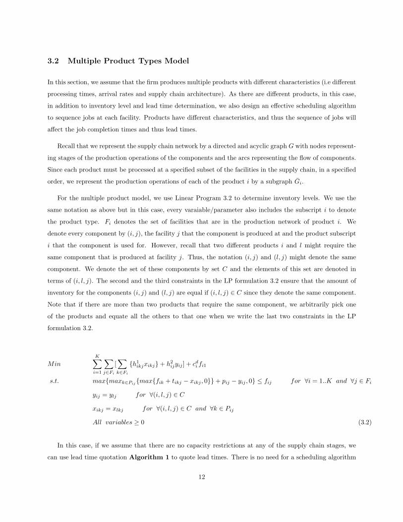
3.2 Multiple Product Types Model
In this section, we assume that the firm produces multiple products with different characteristics (i.e different
processing times, arrival rates and supply chain architecture). As there are different products, in this case,
in addition to inventory level and lead time determination, we also design an effective scheduling algorithm
to sequence jobs at each facility. Products have different characteristics, and thus the sequence of jobs will
affect the job completion times and thus lead times.
Recall that we represent the supply chain network by a directed and acyclic graph G with nodes represent-
ing stages of the production operations of the components and the arcs representing the flow of components.
Since each product must be processed at a specified subset of the facilities in the supply chain, in a specified
order, we represent the production operations of each of the product i by a subgraph Gi.
For the multiple product model, we use Linear Program 3.2 to determine inventory levels. We use the
same notation as above but in this case, every varaiable/parameter also includes the subscript i to denote
the product type. Fi denotes the set of facilities that are in the production network of product i. We
denote every component by (i, j), the facility j that the component is produced at and the product subscript
i that the component is used for. However, recall that two different products i and l might require the
same component that is produced at facility j. Thus, the notation (i, j) and (l, j) might denote the same
component. We denote the set of these components by set C and the elements of this set are denoted in
terms of (i, l, j). The second and the third constraints in the LP formulation 3.2 ensure that the amount of
inventory for the components (i, j) and (l, j) are equal if (i, l, j) ∈ C since they denote the same component.
Note that if there are more than two products that require the same component, we arbitrarily pick one
of the products and equate all the others to that one when we write the last two constraints in the LP
formulation 3.2.
Min
K∑
i=1
∑
j∈Fi
[∑
k∈Fi
{h1ikjxikj}+ h2
ijyij ] + cdi fi1
s.t. max{maxk∈Pij{max{fik + tikj − xikj , 0}}+ pij − yij , 0} ≤ fij for ∀i = 1..K and ∀j ∈ Fi
yij = ylj for ∀(i, l, j) ∈ C
xikj = xlkj for ∀(i, l, j) ∈ C and ∀k ∈ Pij
All variables ≥ 0 (3.2)
In this case, if we assume that there are no capacity restrictions at any of the supply chain stages, we
can use lead time quotation Algorithm 1 to quote lead times. There is no need for a scheduling algorithm
12

since there is no capacity constraint and each arriving job is immediately processed at each stage without
waiting.
However, when we model restricted capacity and assume that there is a single server (or M < ∞ servers)
at a facility), then there will be congestion and queues in the system. In this case, we approximate the
waiting time of orders at facility j using an approach similar to the one we employed for the single product
model. For the schedule used at facility j, we find the expected waiting time of an order type i in that queue
with arrival rate Dij and processing time pij . In this case, the expected waiting time for type i at facility j,
E[Wij ], depends on the schedule used at that facility and on orders for other products at the facility. We
find the mean waiting time of jobs of type i at facility j, E[Wij ], and use these values in the place of pij in
the LP formulation 3.2. Note that, E[Wij ] depends on the schedule used in the system. Thus, depending on
the schedule used, we approximate E[Wij ] values using existing results for expected waiting times of jobs in
an M/D/1 queue with multiple product types. For example, see Wallstrom [24] and Conway et al. [2] for
the calculation of the expected waiting times in the system in an M/G/1 queue with multiple product types
for FCFS and SPTA scheduling rules.
We also use a lead time quotation approach similar to the one presented in Algorithm 2. However,
in this case, the jobs aren’t necessarily sequenced FCFS at each facility. Recall that, in order to minimize
objective function (2.1), we first want to minimize the waiting time component by employing an effective
scheduling algorithm. Thus, we want to find a scheduling algorithm to minimize the total waiting times, and
since completion time of a job is equal to the arrival time of that job to the system plus the waiting time in
the system, we want to minimize the total completion times. Although the simplest case of this problem,
the problem of minimizing total completion times at a single facility is shown to be NP-Hard, Kaminsky and
Simchi-Levi [14] show that the SPTA (Shortest Processing Time Available) rule is asymptotically optimal
(i.e optimal as the number of jobs go to ∞) for this problem. Under the SPTA heuristic, each time a job
completes processing, the shortest available job which has yet not been processed is selected for processing.
Also, note that this approach to sequencing does not take quoted lead times into account, and is thus easily
implemented.
We found in Kaya and Kaminsky [18, 19] that using SPTA at the supplier and FCFS at the manufacturer
is effective in minimizing total completion times for a two facility supply chain. Indeed, Xia, Shantikumar
and Glynn [25] and Kaminsky and Simchi-Levi [17] independently proved that for a flow shop model with
n machines, if the processing times of a job on each of the machines are independent and exchangeable,
processing the jobs according to the shortest total processing time pi =∑n
j=1 pij at the first facility and on
a FCFS basis at the others is asymptotically optimal if all the release times are 0.
13

Thus, we consider sequencing orders FCFS and SPTA at each of the facilities. If FCFS schedule were
used at all facilities, then Algorithm 2 would be effective for quoting lead times. However, if an SPTA
based schedule is used at a facility, then we need to consider future arrivals in addition to the current state
of the system because future arrivals might be scheduled before jobs currently in the queue, and thus delay
the delivery times of those jobs.
Based on these ideas, we present the following scheduling algorithm for this system. For each product
type i, on the production graph Gi, we find the longest path from the manufacturer to the end supplier,
where arc lengths between two nodes j and k is lijk = pij + tijk and then we find the total processing time
of each product type i by summing all the arc lengths on this path. Then, we schedule the jobs according
to shortest total processing times at the facilities that don’t have any internal suppliers in the whole supply
chain network and use a FCFS schedule at all the other facilities. Based on this schedule, we design a
lead time quotation algorithm using the approach introduced in Kaminsky and Kaya [18]. We detail this
scheduling and lead time quotation approach below in Algorithm 3.
In this system let δi denote the arrival probabilities for each product type i = 1..K with sum equal
to 1. Let set Mi denote the set of product types that are going to be scheduled before product type i
and ψi =∑
k∈Miδk be the probability that an arriving job is going to be scheduled before job type i.
µij =∑
k∈Mi{δkpkj} is the expected processing time of such a job at facility j and λ is the mean inter-
arrival time of orders. Recall that since there are inventories in the system, another job l of type i, that is
already in the system at time ro might be used to satisfy order o of type i. In Algorithm 3, U lj denotes the
set of jobs in front of job l in the queue of facility j at time ro, N lj denotes the approximated number of orders
that will arrive after order o but will be scheduled before job l at facility j, wlj denotes the approximated
waiting time of job l at facility j and dlj denotes the completion time of job l at facility j. Then, the
scheduling and lead time quotation algorithm for an order o of type i is detailed below in Algorithm 3,
where the notation is the same as in the LP formulation 3.2:
14
ALGORITHM 3:
Scheduling:
Step 1: Find the total time required to process each product type i (i.e. the longest path from
the suppliers at the end of the chain to the manufacturer for product type i where arc
length between two nodes j and k is lijk = pij + tijk) and denote it by Ti.
Step 2: Define set L to be set of facilities that have no internal supplier. Whenever a facility
j ∈ L is available, process the job type i with shortest Ti and use FCFS schedule at
other facilities j /∈ L.
Lead Time Quotation:
Step 3: Form the subgraph G′i of Gi as in Algorithm 2 and set N lj = 0 for ∀j
Step 4: For ∀j ∈ G′i: if j ∈ S, then put facility j in set F
Step 5: For ∀j ∈ G′i
If j ∈ E then dlj = fj
If j ∈ S and j has no predecessor in the production network of type i, then delete
facility j from set F and
wlj = summ∈U l
jpm
j
slacklj =
min{ wljψiµi
j
λ−ψiµij, (n− l)ψiµ
ij} if λ− ψiµ
ij > 0
(n− l)ψiµij otherwise
N lj = slackl
j/µij
dlj = pi
j + wlj + slackl
j
Step 6: For ∀j ∈ G′i, if j ∈ F and k /∈ F for ∀k ∈ Pij , then delete facility j from set F and
If facility j ∈ L, then
wlj = max{summ∈U l
jpm
j −maxk∈Pij{dlk + tlkj}, 0}
slacklj =
min{ wljψiµi
j
λ−ψiµij, (n− l)ψiµ
ij} if λ− ψiµ
ij > 0
(n− l)ψiµij otherwise
N lj = slackl
j/µij
dlj = maxk∈Pij{dl
k + tlkj}+ pij + wl
j + slacklj
If facility j /∈ L
N lj = maxk∈Pij N
lk
wlj = max{summ∈U l
jpm
j + maxk∈Pij{N lk}µi
j −maxk∈Pij{dlk + tlkj}, 0}
dlj = maxk∈Pij{dl
k + tlkj}+ plj + wl
j
Step 7: Stop if set F is empty and set do = dl1 as the lead time for order o.
Return to step 6 otherwise.
15

E1 20
5
0.5
3
1.2
1.5
10
1 E2 30
S2 15 1
8
1.5 S1 10 1
4
2
S3 6
1.8
12
3.5 S4 30 3
120
151.5
S5 15
1.2
S6 10 8
Figure 2: Supply Chain Network Example
tij
hij1
Fi pi hi
2 Fj pj
Figure 3: Explanation of the values
4 Computational Study
We performed a variety of computational experiments in order to evaluate the performance of our algorithms,
both when compared to traditional approaches for these same problems, and when compared to lower bounds
on optimal solutions for our models. We do an extensive simulation study utilizing a supply chain network
with different processing times, transshipment times between facilities, unit holding costs and unit waiting
costs and implement our heuristics in C++. Whenever needed, we solve the LP model 3.1 or 3.2 using ILOG
AMPL/CPLEX 7.0.
We use the supply chain network as shown in Figure 2. The meanings of the numbers in Figure 2 are
explained in Figure 3. In the picture 2, Si denotes the facilities that belong to the same firm and Ei denotes
the external suppliers.
4.1 Effect of Inventory Positioning for Uncapacitated Systems
We first consider the uncapacitated single product case where the waiting time of a job at facility j is
deterministic and equal to pj (e.g. an infinite server model). As we discussed in Section 2, since, the demand
16
is stochastic, the firm needs to keep some safety stock to achieve the desired service level. In Table 1, we
compare the optimal objective values of the formulation 3.1 with inventory held at every facility as opposed
to the same objective function when holding no inventory at all or holding only finished good inventories.
The ratios of the objective function values of formulation 3.1 with the combined strategy over the costs with
pure MTS and MTO strategies for different combinations of inventory holding cost at the manufacturer, h,
and unit lead time cost, cd are shown in Table 1. The values in Table 1 illustrate the importance of effective
inventory placement in supply chains, although these specific values clearly depend on the holding costs at
each of the facilities. In the following sections, we also make the same comparison using a simulation analysis
of the system.
As we have discussed, firms traditionally use either an MTO strategy (with no inventory) or an MTS
strategy keeping only finished goods inventory. However, as we show in Table 1 using the objective function
of LP 3.1, a combined strategy is clearly much better than these pure strategies for minimizing the total
inventory plus lead time costs for the uncapacitated system. For example, when holding costs are as given
in Figure 2 with the exception of holding cost for finished goods at the last facility, which is 4 (h = 4) and
cd = 5, with a pure MTS strategy (with lead time 0) we need to keep a finished goods inventory of 95 units
with a cost of 380. With a pure MTO strategy, the lead time will be 95 and the cost is 475. However, with
a combined strategy with yS1 = 10, yS2 = 15, yS4 = 12, yS6 = 40, xE1,S2 = 25, xE2,S5 = 40 xS1,S4 = 20
xS2,S4 = 3, the total cost will be 307.1. The cost of the combined strategy is significantly lower than the
costs of either pure strategy.
We consider another example, in which the target lead time is 30 and we try to achieve this lead time
by holding inventory. If we only keep finished goods inventory, then yS6 = 65 and the total inventory cost is
260. However, by keeping inventory at other facilities, with the same lead time, the total inventory cost can
be decreased to 187.1 with yS1 = 10, yS2 = 15, yS6 = 22, xE1,S2 = 25, xE2,S5 = 28 xS1,S4 = 20 xS2,S4 = 3.
In addition, we will be able to cut the lead time by half to 15 at a cost of 247.1 which is even less than the
cost with the initial strategy.
We see that as the unit inventory holding cost at the manufacturer, h, increases or the unit lead time cost,
cd, decreases, an MTO strategy gives results closer to those of the combined strategy, and as h decreases
or cd increases, the MTS strategy becomes more effective. Also, increasing cd (or h) beyond a certain level
doesn’t impact the system because the lead time (or finished goods inventory) in the optimal solution is
optimally set to 0 for cd (or h) high enough, so increasing cd (or h) further won’t affect the system (assuming
that everything else remains the same).
17
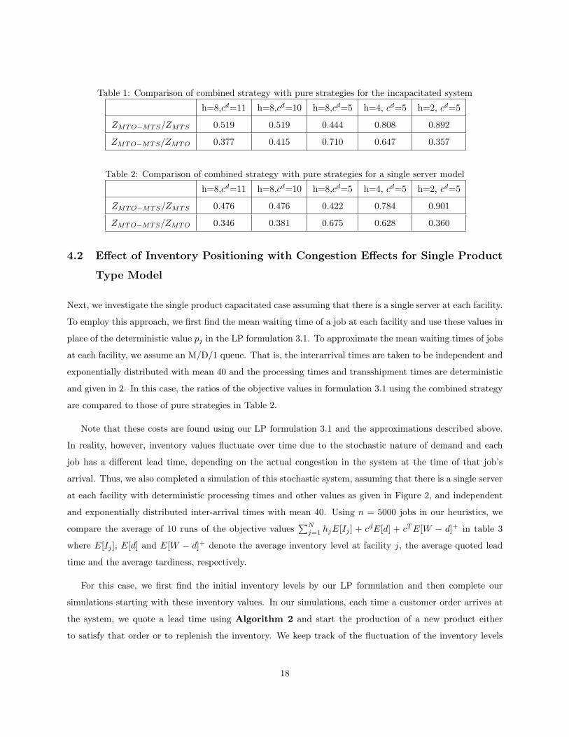
Table 1: Comparison of combined strategy with pure strategies for the incapacitated system
h=8,cd=11 h=8,cd=10 h=8,cd=5 h=4, cd=5 h=2, cd=5
ZMTO−MTS/ZMTS 0.519 0.519 0.444 0.808 0.892
ZMTO−MTS/ZMTO 0.377 0.415 0.710 0.647 0.357
Table 2: Comparison of combined strategy with pure strategies for a single server model
h=8,cd=11 h=8,cd=10 h=8,cd=5 h=4, cd=5 h=2, cd=5
ZMTO−MTS/ZMTS 0.476 0.476 0.422 0.784 0.901
ZMTO−MTS/ZMTO 0.346 0.381 0.675 0.628 0.360
4.2 Effect of Inventory Positioning with Congestion Effects for Single Product
Type Model
Next, we investigate the single product capacitated case assuming that there is a single server at each facility.
To employ this approach, we first find the mean waiting time of a job at each facility and use these values in
place of the deterministic value pj in the LP formulation 3.1. To approximate the mean waiting times of jobs
at each facility, we assume an M/D/1 queue. That is, the interarrival times are taken to be independent and
exponentially distributed with mean 40 and the processing times and transshipment times are deterministic
and given in 2. In this case, the ratios of the objective values in formulation 3.1 using the combined strategy
are compared to those of pure strategies in Table 2.
Note that these costs are found using our LP formulation 3.1 and the approximations described above.
In reality, however, inventory values fluctuate over time due to the stochastic nature of demand and each
job has a different lead time, depending on the actual congestion in the system at the time of that job’s
arrival. Thus, we also completed a simulation of this stochastic system, assuming that there is a single server
at each facility with deterministic processing times and other values as given in Figure 2, and independent
and exponentially distributed inter-arrival times with mean 40. Using n = 5000 jobs in our heuristics, we
compare the average of 10 runs of the objective values∑N
j=1 hjE[Ij ] + cdE[d] + cT E[W − d]+ in table 3
where E[Ij ], E[d] and E[W − d]+ denote the average inventory level at facility j, the average quoted lead
time and the average tardiness, respectively.
For this case, we first find the initial inventory levels by our LP formulation and then complete our
simulations starting with these inventory values. In our simulations, each time a customer order arrives at
the system, we quote a lead time using Algorithm 2 and start the production of a new product either
to satisfy that order or to replenish the inventory. We keep track of the fluctuation of the inventory levels
18

Table 3: Simulation analysis of combined strategy compared to pure strategies
h=8,cd=11 h=8,cd=10 h=8,cd=5 h=4, cd=5 h=2, cd=5
ZMTO−MTS/ZMTS 0.833 0.833 0.810 0.892 0.944
ZMTO−MTS/ZMTO 0.723 0.785 0.871 0.827 0.651
Table 4: Comparison of lead times and due dates to actual waiting times and completion times
n=10 n=100 n=1000 n=5000
ZnW /Zn
LT 0.891 0.950 0.964 0.962
ZnC/Zn
DD 0.925 0.967 0.992 0.996
over time at each facility and calculate the average inventory costs with the average quoted lead time and
tardiness costs. We compare the objective functions∑N
j=1 hjE[Ij ]+cdE[d]+cT E[W−d]+ with this combined
model to the same objective function with pure MTO and MTS models. The initial inventories are all 0 for
the MTO model and there is only finished goods inventory for the MTS model. The ratios of the costs are
presented in Table 3 for different h and cd combinations with cT = 12.
To assess the effectiveness of lead time quotation Algorithm 2, we also compare the lead times quoted
for this single type system to the actual waiting times of the jobs in the system using cd = 5 and cT = 7. Let
ZnLT =
∑ni=1{cddi + cT (Wi − di)+} denote the total lead time plus tardiness costs, Zn
DD = ZLT +∑n
i=1 ri
denote the total due dates plus tardiness costs, ZnW =
∑ni=1{cdWi} denote the total waiting times of the
jobs in the system and ZnC = ZW +
∑ni=1 ri denote the total completion times of the jobs. We present ratios
for these values for different number of jobs, n, in Table 4. As we see in Table 4, the lead times quoted with
Algorithm 2 are very close to the actual waiting times and ZnDD approach to Zn
C as n gets bigger.
4.3 Effectiveness of the Algorithms for Multiple Product Types
We also designed a simulation study using a system with multiple product types to assess the effectiveness
of our algorithms. In addition to the single product type we considered in the previous section, now we
use 4 additional product types with arrival probabilities and processing times as shown in Table 5. In our
model, all of the products have the same supply chain architecture and they all need to be processed at all
of the facilities in Figure 2. Also, we use equal transshipment times and inventory holding costs for each of
the products and they are as shown in Figure 2. The inter-arrival times are taken to be independent and
exponentially distributed with mean 40. We average of 10 trials, each with n = 5000 jobs, and present the
averages of these runs in the following tables.
19

Table 5: Arrival probabilities and mean processing times of product types
δl pE1 pE2 pS1 pS2 pS3 pS4 pS5 pS6
l=1 0.2 20 30 10 15 6 30 15 10
l=2 0.3 15 10 25 5 45 15 20 10
l=3 0.15 5 15 10 10 15 20 25 15
l=4 0.25 10 20 30 15 10 5 10 20
l=5 0.1 20 5 5 10 5 10 30 15
We first consider 3 different product types using the first three product types in Table 5 and then 5
different product types considering all the products in table 5. For the arrival probability of type l = 1, we
use 0.55 in 3-product type model instead of 0.2 so that the sum of the arrival probabilities of all types will
be 1.
We use the scheduling and lead time quotation approach detailed in Algorithm 3. To explore the
effectiveness of the SPTA schedule, we compared the total waiting times of jobs using the SPTA schedule
to that of a lower bound. If we consider only the bottleneck facility (the facility with slowest processing
rate), use an SPTA schedule with preemption in that facility, and assume that the waiting time of any job
in the queue of any other facility is zero, then the total weighted waiting time of jobs at this system will
be a lower bound for those in our model. Let ZLB denote the lower bound for the total weighted waiting
times of jobs in the system and ZSPTA =∑n
i=1{cdWi} denote the total weighted waiting times with the
SPTA-based schedule. The comparison of the total waiting times resulting from the use of our heuristic to
that of the lower bound is presented in Table 6 for different numbers of jobs. Also, to explore the effectiveness
of the LTQ part of Algorithm 3, we present the ratios of the total quoted lead times plus tardiness costs,
ZSPTA−LTQ =∑n
i=1{cddi + cT (Wi−di)+} for this case over ZSPTA and ZLB in Table 6 using equal weights
for different product types, cd = 5 and cT = 7. Note that the optimal off-line LTQ algorithm quotes lead
times that are exactly equal to the waiting times of the jobs in the system which is equal to ZSPTA, thus
ZSPTA is a lower bound for the LTQ algorithm with the SPTA-based schedule and ZLB is a lower bound
among all schedules. As seen in this table, the difference between ZSPTA and the lower bound is less than
20% and the lead time quotation algorithm gives results that are less than 7% worse than ZSPTA. Thus, we
conclude that our scheduling and lead time quotation Algorithm 3 is effective in minimizing the objective
function∑n
i=1{cddi + cT (Wi − di)+}
In Table 7, using cT = 12 and different weights for h and cd, we present the ratios of the total costs∑K
i=1{(∑N
j=1 hijE[Iij ]) + cdi E[di] + cT
i E[Wi − di]+} with our heuristics to that of the total costs with pure
MTO and MTS strategies and the total costs using a FCFS schedule. In this simulation study, according
20

Table 6: Comparison of SPTA schedule and the LTQ with the lower bound for K=3 and K=5 product types
K=3 n=10 n=100 n=1000 n=5000 K=5 n=10 n=100 n=1000 n=5000
ZLB/ZSPTA 0.962 0.813 0.847 0.833 0.859 0.790 0.822 0.816
ZSPTA/ZLT 0.874 0.933 0.952 0.947 0.941 0.922 0.925 0.931
ZLB/ZLT 0.848 0.753 0.802 0.786 0.807 0.735 0.766 0.751
Table 7: Comparison of combined strategy with pure strategies for multiple product type models
K=3 h=8,cd=11 h=8,cd=10 h=8,cd=5 h=4, cd=5 h=2, cd=5
ZMTO−MTS/ZMTS 0.732 0.732 0.695 0.887 0.936
ZMTO−MTS/ZMTO 0.603 0.666 0.851 0.789 0.628
ZSPTA/ZFCFS 0.934 0.943 0.918 0.930 0.956
K=5 h=8,cd=11 h=8,cd=10 h=8,cd=5 h=4, cd=5 h=2, cd=5
ZMTO−MTS/ZMTS 0.762 0.762 0.717 0.869 0.939
ZMTO−MTS/ZMTO 0.693 0.724 0.871 0.812 0.687
ZSPTA/ZFCFS 0.861 0.885 0.874 0.891 0.925
to our heuristic, we first find the inventory values using our LP formulation 3.2 and then use the scheduling
and lead time quotation algorithm as explained in Algorithm 3. As we see in Table 7, the costs with the
combined strategy is about 20% less on average than the pure strategies. Also, the SPTA based schedule
used for this model decreases the total costs by about 10% compared to a FCFS schedule. Also, we see that
as cd decreases, the combined system moves toward a MTO system while as h decreases, MTS system gives
better results.
We also analyze the impact of the congestion level on the system performance. We present the results in
Table 8 using 5 different product types with the same supply chain structure and with arrival probabilities
and processing times as given in Table 5 and using weights h = 4, cd = 5 and cT = 7. We increase the demand
rate, and thus the congestion level at each facility, gradually from 1/40 to 1/20. The congestion levels in Table
8 denote the congestion levels at the bottleneck facility (i.e. the most congested facility) calculated by using
the arrival probabilities and processing times in Table 5 and the demand rates in Table 8 for each facility.
Observe that the MTS system gives better results as congestion increases and the MTO system performs
significantly better if the congestion decreases. Also, observe that the SPTA based schedule as explained
in Algorithm 3 performs much better than the FCFS schedule as the congestion increases, although the
performance of the SPTA based schedule diverges from the lower bound as the congestion increases. In
addition, we see that the lead time quotation algorithm performs very well even if the congestion level is
21

Table 8: Effect of demand rate and congestion level in the system
Demand Rate Congestion Level ZMT O−MT S
ZMT S
ZMT O−MT S
ZMT O
ZSP T A
ZF CF S
ZLB
ZSP T A
ZSP T A
ZLT
1/20 0.99 0.898 0.685 0.852 0.795 0.927
1/25 0.80 0.869 0.812 0.891 0.816 0.921
1/30 0.66 0.878 0.856 0.902 0.834 0.942
1/35 0.57 0.862 0.887 0.917 0.867 0.949
1/40 0.50 0.857 0.912 0.945 0.901 0.963
12
3.5
S2 30 3
S1 10 4
12
2.5
S3 30 2
45
0.5
S4 5 1
2
1.5
S5 35 0.2
Figure 4: Structure 1: 4-supplier flow shop model
very high. This is primarily due to the fact that when congestion is high, the inventory levels are also high,
so that when an order arrives, we can frequently satisfy it from inventory so there is no error in lead time
quotation.
4.4 Effect of Supply Chain Structure on the System
We also study the effect of supply chain structure on the system and on the effectiveness of our heuristics. For
this purpose, we consider the supply chain structures shown in Figures 4 - 8, moving from serial to parallel
facility models. We complete a set of simulations using these supply chain structures. We use the appropriate
LP formulation to determine target inventory levels, and then use Algorithm 3 during the simulation to
schedule and quote due dates. In Table 10, we compare the total costs Z =∑K
i=1{(∑N
j=1 hijE[Iij ]) +
cdi E[di] + cT
i E[Wi − di]+} when our heuristic is used to the total costs with pure MTO and MTS strategies,
and the total costs using an FCFS schedule with a mixed strategy.
Processing times for product type l = 1, transshipment times, and unit holding costs, are shown on the
graphs. We consider 4 additional product types with the arrival probabilities and processing times shown
in Table 9. The transshipment and unit holding costs for different product types are equal and as shown on
the graphs. The order inter-arrival times are taken to be independent and exponentially distributed with
mean 40 and unit tardiness cost cT = 8. We consider two possible unit lead time costs, cd = 5 and cd = 3.3.
Each entry in Table 10 is the average of 10 simulation runs with n = 5000 jobs in each run.
As can be seen in Table 10, the combined MTS-MTO approach performs significantly better than pure
22

12
3.5
S2 30 3
S1 10 4
12
2.5
S3 30 2
Figure 5: Structure 2: 2-supplier flow shop model
12
3.5
S2 30 3
S1 10 4
Figure 6: Structure 3: Single supplier, single manufacturer model
12 2.5
S3 30
2
12 3.5
S2 30 3
S1 10 4
Figure 7: Structure 4: 2 parallel supplier model
2
0.5
S5 35 0.2
12
1.5
S4 5
1
S1 10 4
3
S3 30
2
S2 30
2.5 12
45
3.5
Figure 8: Structure 5: 4 parallel supplier model
23
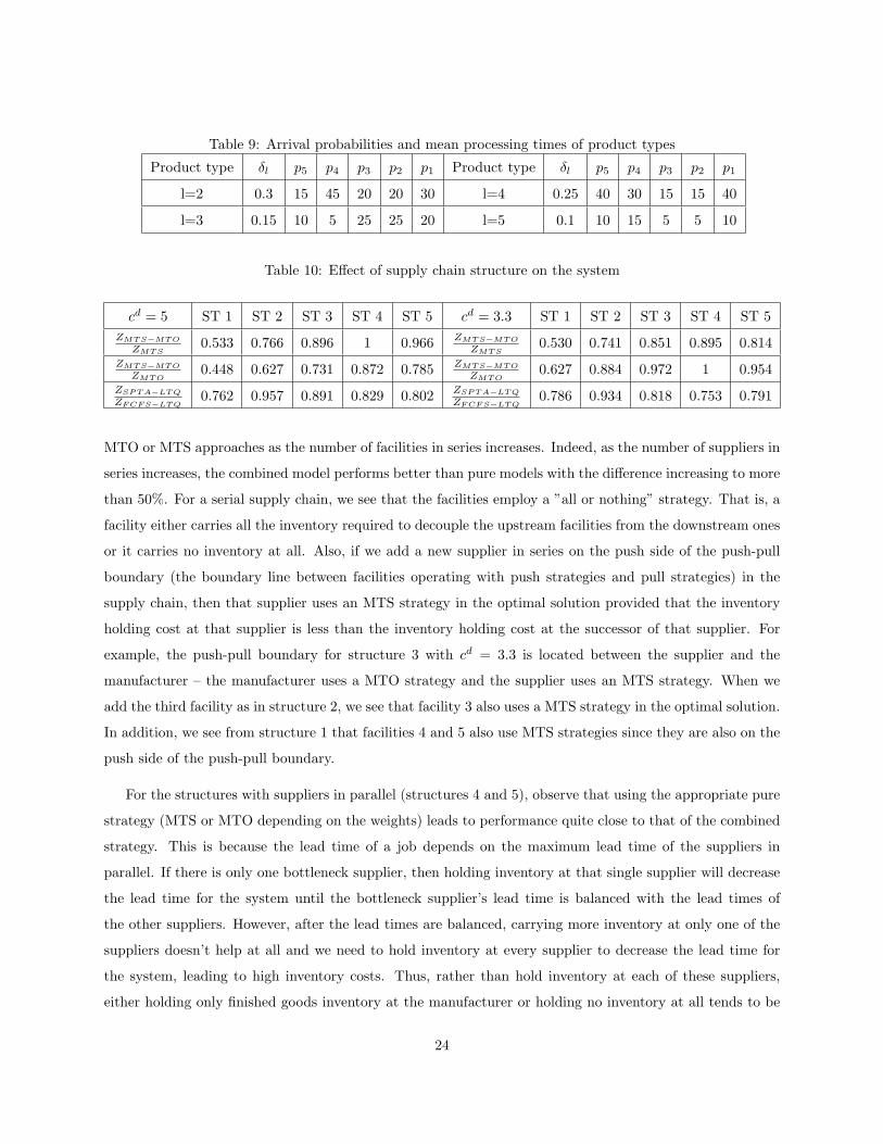
Table 9: Arrival probabilities and mean processing times of product types
Product type δl p5 p4 p3 p2 p1 Product type δl p5 p4 p3 p2 p1
l=2 0.3 15 45 20 20 30 l=4 0.25 40 30 15 15 40
l=3 0.15 10 5 25 25 20 l=5 0.1 10 15 5 5 10
Table 10: Effect of supply chain structure on the system
cd = 5 ST 1 ST 2 ST 3 ST 4 ST 5 cd = 3.3 ST 1 ST 2 ST 3 ST 4 ST 5ZMT S−MT O
ZMT S0.533 0.766 0.896 1 0.966 ZMT S−MT O
ZMT S0.530 0.741 0.851 0.895 0.814
ZMT S−MT O
ZMT O0.448 0.627 0.731 0.872 0.785 ZMT S−MT O
ZMT O0.627 0.884 0.972 1 0.954
ZSP T A−LT Q
ZF CF S−LT Q0.762 0.957 0.891 0.829 0.802 ZSP T A−LT Q
ZF CF S−LT Q0.786 0.934 0.818 0.753 0.791
MTO or MTS approaches as the number of facilities in series increases. Indeed, as the number of suppliers in
series increases, the combined model performs better than pure models with the difference increasing to more
than 50%. For a serial supply chain, we see that the facilities employ a ”all or nothing” strategy. That is, a
facility either carries all the inventory required to decouple the upstream facilities from the downstream ones
or it carries no inventory at all. Also, if we add a new supplier in series on the push side of the push-pull
boundary (the boundary line between facilities operating with push strategies and pull strategies) in the
supply chain, then that supplier uses an MTS strategy in the optimal solution provided that the inventory
holding cost at that supplier is less than the inventory holding cost at the successor of that supplier. For
example, the push-pull boundary for structure 3 with cd = 3.3 is located between the supplier and the
manufacturer – the manufacturer uses a MTO strategy and the supplier uses an MTS strategy. When we
add the third facility as in structure 2, we see that facility 3 also uses a MTS strategy in the optimal solution.
In addition, we see from structure 1 that facilities 4 and 5 also use MTS strategies since they are also on the
push side of the push-pull boundary.
For the structures with suppliers in parallel (structures 4 and 5), observe that using the appropriate pure
strategy (MTS or MTO depending on the weights) leads to performance quite close to that of the combined
strategy. This is because the lead time of a job depends on the maximum lead time of the suppliers in
parallel. If there is only one bottleneck supplier, then holding inventory at that single supplier will decrease
the lead time for the system until the bottleneck supplier’s lead time is balanced with the lead times of
the other suppliers. However, after the lead times are balanced, carrying more inventory at only one of the
suppliers doesn’t help at all and we need to hold inventory at every supplier to decrease the lead time for
the system, leading to high inventory costs. Thus, rather than hold inventory at each of these suppliers,
either holding only finished goods inventory at the manufacturer or holding no inventory at all tends to be
24

more profitable, depending on the unit weights. For example, for structure 4, using a pure MTS strategy is
optimal when cd = 5 > hS1 = 4 and a pure MTO strategy is optimal when cd = 3.3 < hS1 = 4 since carrying
inventory at only one of the suppliers doesn’t help the system.
We also found that Algorithm 3 which is based on SPTA schedule performs about 15% better on
average than the algorithm in which we schedule all the jobs according to FCFS at all the facilities and
quote lead times accordingly. Recall that the difference in performance appears to depend primarily on the
processing times of the product types at different facilities, and appears not to be significantly impacted by
supply chain structure.
5 Conclusion
In this paper, we consider stylized models of complex MTO-MTS supply chains in a stochastic, multi-
item environment and designed effective algorithms for inventory placement, job scheduling, and lead time
quotation. We completed a computational analysis and found that combined MTO-MTS systems perform
significantly better than pure MTO or MTS systems, and that an SPTA based algorithm for scheduling the
jobs performs much better than the generally used FCFS approach. We also explored the effect of supply
chain structure and several other parameters on the supply chain performance.
Of course, these are stylized models, and real world supply chains have many complex characteristics
that are not captured by these models. Nevertheless, this is to the best of our knowledge, the first study
that explores inventory positioning, scheduling and lead-time quotation together in the context of a supply
chain.
In the future, we intend to expand this research to consider different functions of lead time in the objective
function. In some systems, the manufacturer doesn’t have to accept all orders and has the option to reject
certain orders. Similarly, the customers might choose not to place an order to the system depending on the
quoted lead time. Pricing and capacity decisions can also be incorporated into these models. Also, contracts
and gaming strategies might also be analyzed for these systems. In all of these models and variants, the
manufacturer needs to develop strategies for system design, and for scheduling and lead time quotation.
References
[1] Axsater, S. (1993), Continuous Review Policies for Multi-level Inventory Systems with Stochastic
Demand. S.C. Graves, A.H. Rinnoy Kan and P.H. Zipkin eds. Handbooks in Oper. Res. and Man-
25
agement Sci. Vol 4. Logistics of Production and Inventory North Holland Publishing Company,
Amsterdam, The Netherlands. Chapter 4.
[2] Conway R., W. Maxwell and L. Miller (1967). Theory of Scheduling.Addison-Wesley Publishing
Company, Reading, MA.
[3] Diks E.B., A.G. de Kok, A.G. Lagodimos (1996), Multi-Echelon Systems: A Service Measure Per-
spective European Journal of Oper. Res. 95 pp. 241-263.
[4] Ettl M., G.E. Feigin, G.Y. Lin, D.D. Yao (2000), A Supply Network Model with Base-Stock Control
and Service Requirements Operations Research 48
[5] Federgruen A. (1993), Centralized Planning Models for Multi-Echelon Inventory Systems under
Uncertainty. S. C. Graves, A. H. Rinnooy Kan, P. H. Zipkin, eds. Handbooks in Operations Research
and Management Science, Vol 4., Logistics of Production and Inventory, North-Holland Publishing
Company, Amsterdam, The Netherlands, Chapter 3.
[6] Glasserman, P., S. Tayur. (1995). Sensitivity Analysis for Base-Stock Levels in Multi-echelon
Production-Inventory Systems Management Sci. 41 pp. 263281.
[7] Graves S.C., S.P. Willems (1996), Strategic Safety Stock Placement in Supply Chains, Proceedings
of the 1996 MSOM Conference, Hanover, NH.
[8] Graves S.C., S.P. Willems (2000). Optimizing Strategic Safety Stock Placement in Supply Chains
Manufacturing and Service Operations Management 2 pp. 68-83.
[9] Graves S.C., S.P. Willems (2003), Erratum: Optimizing Strategic Safety Stock Placement in Supply
Chains, Manuf. Serv. Oper. Manage. 5 pp. 176177.
[10] Inderfurth, K. (1991). Safety Stock Optimization in Multi-Stage Inventory Systems. International
Journal of Production Econom. 24 pp. 103113.
[11] Inderfurth, K. (1993). Valuation of Leadtime Reduction in Multi-Stage Production Systems. G. Fan-
del, T. Gulledge, A. Jones, eds. Oper. Res. in Production Planning and Inventory Control Springer,
Berlin, Germany, pp. 413427.
[12] Inderfurth, K. (1994). Safety Stocks in Multistage, Divergent Inventory Systems: A survey. Inter-
national J. of Production Economics 35 pp. 321329.
[13] Inderfurth, K., S. Minner. (1998). Safety Stocks in Multi-Stage Inventory Systems under Different
Service Measures. European J. Oper. Res. 106 pp. 57 73.
26

[14] Kaminsky, P. and D. Simchi-Levi (2001), Probabilistic Analysis of an On-line Algorithm for the
Single Machine Completion Time Problem with Release Dates. Operations Research Letters 29 pp.
141-148.
[15] Lee, H. L., C. Billington. (1993). Material Management in Decentralized Supply Chains. Operations
Research, 41 pp. 835847.
[16] Lee, H., P. Padmanabhan and S. Whang (1997) Information Distortion in a Supply Chain: The
Bullwhip Effect Management Science 43, pp. 546-558.
[17] Kaminsky, P. and D. Simchi-Levi (1998), Probabilistic Analysis and Practical Algorithms for the
Flow Shop Weighted Completion Time Problem. Operations Research, 46, pp. 872-882.
[18] Kaya, O. and P. Kaminsky (2006), Scheduling and Due Date Quotation in a MTO Supply Chain.
Submitted for Publication.
[19] Kaya, O. and P. Kaminsky (2006), An Analysis of a Combined Make-to-Order/Make-to-Stock Sys-
tem. Working Paper.
[20] Kaya, O. (2006) MTO-MTS Production Systems in Supply Chains. PhD Thesis, University of
California, Berkeley, USA.
[21] Magnanti T.L., Z.M. Shen, J. Shu, D. Simchi-Levi, C.P. Teo (2006). Inventory Placement in Acyclic
Supply Chain Networks Operations Research Letters 34 pp. 228-238.
[22] Minner, S. (1997). Dynamic Programming Algorithms for Multi-Stage Safety Stock Optimization.
OR Spektrum 19 pp. 261271.
[23] Simpson, K. F. (1958). In-process Inventories. Operations Research, 6 pp. 863873.
[24] Wallstrom, B. (1980). On the M/G/1 queue with several classes of customers having different service
time distributions, Report 1-19, Lund Institute of Technology.
[25] Xia, C., G. Shanthikumar, and P. Glynn (2000), On The Asymptotic Optimality of The SPT Rule
for The Flow Shop Average Completion Time Problem. Operations Research 48, pp. 615-622.
27


![Slew/Translation Positioning and Swing …liberzon.csl.illinois.edu/teaching/SlewTranslation...scheduling feedback-based control schemes for tower crane systems [40], [41]. In [42],](https://img.pdfslide.net/doc/110x75/5f1d71b0bf5094161d61b275/slewtranslation-positioning-and-swing-scheduling-feedback-based-control-schemes.jpg)