Embed Size (px)
Citation preview

INTEGRATED MACHINE-SCHEDULING
AND INVENTORY PLANNING OF DOOR
MANUFACTURING OPERATIONS AT
OYAK RENAULT FACTORY
A THESIS
SUBMITTED TO THE DEPARTMENT OF INDUSTRIAL
ENGINEERING
AND THE GRADUATE SCHOOL OF ENGINEERING AND SCIENCE OF
BILKENT UNIVERSITY
IN PARTIAL FULFILLMENT OF THE REQUIREMENTS
FOR THE DEGREE OF
MASTER OF SCIENCE
by
Nurcan Bozkaya
July, 2012

ii
I certify that I have read this thesis and that in my opinion it is full adequate, in scope
and in quality, as a dissertation for the degree of Master of Science.
___________________________________
Assist. Prof. Alper Şen (Advisor)
I certify that I have read this thesis and that in my opinion it is full adequate, in scope
and in quality, as a dissertation for the degree of Master of Science.
___________________________________
Assoc. Prof. Osman Alp (Co-Advisor)
I certify that I have read this thesis and that in my opinion it is full adequate, in scope
and in quality, as a dissertation for the degree of Master of Science.
______________________________________
Assoc. Prof. Mehmet R. Taner (Co-Advisor)
I certify that I have read this thesis and that in my opinion it is full adequate, in scope
and in quality, as a dissertation for the degree of Master of Science.
______________________________________
Assoc. Prof. Osman Oğuz
I certify that I have read this thesis and that in my opinion it is full adequate, in scope
and in quality, as a dissertation for the degree of Master of Science.
______________________________________
Assist. Prof. Sedef Meral
iii
Approved for the Graduate School of Engineering and Science
____________________________________
Prof. Dr. Levent Onural
Director of the Graduate School of Engineering and Science

iv
ABSTRACT
INTEGRATED MACHINE-SCHEDULING AND INVENTORY PLANNING OF
DOOR MANUFACTURING OPERATIONS AT OYAK RENAULT FACTORY
Nurcan Bozkaya
M.S. in Industrial Engineering
Advisor: Assist. Prof Alper Şen
Co-Advisor: Assoc. Prof. Osman Alp
Co-Advisor: Assoc. Prof. Mehmet R. Taner
July, 2012
A car passes through press, body shell, painting and assembly stages during its
manufacturing process. Due to the increased competition among car manufacturers, they
aim to continuously advance and improve their processes. In this study, we analyze
planning operations for the production of front/back and left/right doors in body shell
department of Bursa Oyak-Renault factory and propose heuristic algorithms to improve
their planning processes. In this study, we present four different mathematical models
and two heuristics approaches which decrease the current costs of the company
particularly with respect to inventory carrying and setup perspectives. In the body shell
department of the company, there are two parallel manufacturing cells which produces
doors to be assembled on the consumption line. The effective planning and scheduling
of the jobs on these lines requires solving the problem of integrated machine-scheduling
and inventory planning subject to inclusive eligibility constraints and sequence
independent setup times with job availability in flexible manufacturing cells of the body
shell department. The novelty in the models lie in the integration of inventory planning
and production scheduling decisions with the aim of streamlining operations of the door
manufacturing cells with the consumption line. One of the proposed heuristic

v
approaches is Rolling Horizon Algorithm (RHA) which divides the planning horizon
into sub-intervals and solves the problem by rolling the solutions through sub-intervals.
The other proposed algorithm is Two-Pass Algorithm which divides the planning
horizon into sub-intervals and solves each sub-problem in each sub-interval to optimality
for two times by maintaining the starting and ending inventory levels feasible. These
approaches are implemented with Gurobi optimization software and Java programming
language and applied within a decision support system that supports daily planning
activities.
Keywords: Decision Support System, Integrated Manufacturing System, production
planning and scheduling, car manufacturing.

vi
ÖZET
OYAK RENAULT FABRİKASI KAPI ÜRETİM HATLARINDA ENTEGRE
ENVANTER PLANLAMA VE MAKİNE ÇİZELGELEME OPERASYONLARI
Nurcan Bozkaya
Endüstri Mühendisliği, Yüksek Lisans
Tez Yöneticisi: Yrd. Doç. Dr. Alper Şen
Yardımcı Danışman: Doç. Dr. Osman Alp
Yardımcı Danışman: Doç. Dr. Mehmet R. Taner
Temmuz, 2012
Bir otomobil, üretimi sırasında, özetle pres, kaporta, boya ve montaj aşamalarından
geçmektedir. Otomotiv üreticileri arasındaki artan rekabet koşullarında firma, süreçlerini
sürekli olarak geliştirmek ve iyileştirmek istemektedir. Bu çalışma kapsamında, Bursa
Oyak-Renault fabrikasının kaporta atölyesindeki ön/arka ve sağ/sol kapı üretiminin
planlama operasyonları analiz edilmiş ve planlama süreçlerini iyileştirmek için kesin ve
sezgisel algoritmalar önerilmiştir. Bu çalışmada dört farklı matematiksel model ve
firmanın özellikle envanter taşıma ve kurulum maliyetleri açısından maliyetlerini
düşüren iki sezgisel yaklaşım önerilmiştir. Firmanın kaporta atölyesinde tüketim
hattında araç gövdesine monte edilen kapıların üretimini yapan iki paralel üretim hücresi
bulunmaktadır. Bu hücrelerdeki işlerin etkin bir şekilde planlanması ve çizelgelenmesi,
kaporta atölyesindeki esnek üretim hücrelerinde kapsayan makine atama kısıtlarını, iş
elverişliliği ve sıra-bağımsız kurulum zamanlarını gözönünde bulunduran entegre
makine çizelgeleme ve envanter planlama probleminin çözülmesini gerektirmektedir.
Modellerdeki yenilik, tüketim hattı ile kapı üretim hücrelerindeki operasyonların uygun
hale getirilmesi amacı ile envanter planlama ve üretim çizelgeleme kararlarını entegre
olarak alabilmesinde yatmaktadır.

vii
Önerilen sezgisel yaklaşımlardan biri planlama ufkunu alt-aralıklara bölen ve her bir alt-
aralığı yuvarlayarak çözen “Yuvarlanan Planlama Ufku”dur. Diğer bir yaklaşım ise,
planlama ufkunu alt-aralıklara bölerek her bir alt problemi başlangıç ve bitiş envanter
seviyelerini koruyarak iki kere çözen “İki-Aşamalı Algoritma”dır. Geliştirdiğimiz bu
yaklaşımlar bilgisayar ortamında Gurobi optimizasyon yazılımı ve Java programlama
dili kullanılarak çözüm üretmek üzere işlenmiş, günlük kullanıma elverişli şekilde bir
karar destek sistemi çerçevesinde uygulanmıştır.
Anahtar Kelimeler: Karar Destek Sistemi, Bütünleşik Üretim Sistemi, üretim planlama
ve çizelgeleme, araç imalatı.

viii
To my family…

ix
ACKNOWLEDGEMENT
First and foremost, I would like to express my gratitude to my advisors, Assoc. Prof.
Osman Alp and Assoc. Prof. Mehmet Rüştü Taner. Special thanks to Assoc. Prof.
Osman Oğuz, Assist. Prof. Alper Şen and Assist. Prof. Sedef Meral for their valuable
time and reviews of this thesis.
I would like to thank to my precious friends Fevzi Yılmaz, Müge Muhafız, Onur
Uzunlar and Pelin Elaldı for their endless support, motivation and wholehearted love.
This thesis would not be possible without their help, patience and support. I also wish to
thank Hatice Çalık and Hüsrev Aksüt for their academic assistance and understanding,
and being good friends to me. I am also thankful to all other friends that I failed to
mention here.
I am grateful to The Scientific and Technological Research Council of Turkey
(TUBITAK) and The Ministry of Science Industry and Technology for the financial
support they provided during my research.
It is a pleasure for me to express my deepest gratitude to my dear friends Olcay Kalan
and Gözde Çölek for being such a long time in my life. Their friendship is so valuable
for me.
Last but not the least; I also would like to express my deepest gratitude to my mother
Şükran Bozkaya and father Mehmet Bozkaya for their eternal love, support and trust at
all stages of my life and especially during my graduate study. I especially thank to my
brother, Ercan Bozkaya and his wife Zeliş Bozkaya, for their existence, everlasting love
and morale support during my study.

x
Finally, I am indeed grateful to the love of my life Erdem Özdemir for his endless
support, love and encouragement that he gives from the moment that I met him. This
thesis would not be possible without his help, patience and support.

xi
TABLE OF CONTENTS
Chapter 1 ............................................................................................................................ 1
Introduction .................................................................................................................... 1
Chapter 2 ............................................................................................................................ 3
Problem Definition ......................................................................................................... 3
Chapter 3 .......................................................................................................................... 10
Literature Review ......................................................................................................... 10
2.1. Parallel Machine Scheduling with Eligibility Restrictions ................................ 10
2.2. Scheduling under Sequence Independent Setup Times ..................................... 14
Chapter 4 .......................................................................................................................... 20
Model Development ..................................................................................................... 20
4.1. Case with Idle Times ......................................................................................... 23
4.2. Case with No Idle Times ................................................................................... 29
Chapter 5 .......................................................................................................................... 32
Solution Approaches .................................................................................................... 32
5. 1. Rolling Horizon Algorithm (RHA)................................................................... 33
5. 2. Two-Pass Algorithm (TPA) .............................................................................. 37
Chapter 6 .......................................................................................................................... 42
Computational Results ................................................................................................. 42
6. 1. Test Instances .................................................................................................... 42
6. 2. Computational Results ...................................................................................... 46
6.3. Summary ............................................................................................................ 61

xii
Chapter 7 .......................................................................................................................... 63
Conclusion & Future Directions ................................................................................... 63
Bibliography ..................................................................................................................... 65
APPENDIX ...................................................................................................................... 69
xiii
LIST OF TABLES
Table 3.1 A Summary of the problems on parallel machine scheduling with sequence
independent setup times ................................................................................................... 19
Table 5.1 Notations Used in Rolling Horizon Algorithm ................................................ 35
Table 5.2 Notations used in Two-Pass Algorithm ........................................................... 39
Table 6.1 The parameters of solution methods for the real problems .............................. 43
Table 6.2 The characteristics of Generation Method ....................................................... 44
Table 6.3 The parameters for random problems .............................................................. 46
Table 6.4 Average CPU time and average number of setups found by exact methods
with the same contingency stock and ending inventory levels for real problems with
processing time 2.............................................................................................................. 47
Table 6.5 The average and maximum inventory levels obtained by exact methods for
real problems with processing time 2............................................................................... 47
Table 6.6 Comparison of average CPU time and average number of setups obtained by
TPA and exact methods for real problems with processing time 1 and 2 ....................... 50
Table 6.7 Comparison of average and maximum inventory levels obtained by TPA and
exact methods for real problems with processing time 1 and 2 ....................................... 50
Table 6.8 Comparison of average CPU time and number of setups obtained by TPA and
exact methods for random problems (GM-S1) with processing time 1 and 2 ................. 52
Table 6.9 Comparison of average and maximum inventory levels obtained by TPA and
exact methods for random problems (GM-S1) with processing time 1 and 2 ................. 52
Table 6.10 Comparison of CPU time and number of setups obtained by RHA and exact
methods for real problems with processing time 1 and 2 for average ............................. 53
Table 6.11 Comparison of average and maximum inventory levels obtained by RHA and
exact methods for real problems with processing time 1 and 2 ....................................... 53
Table 6.12 Comparison of average CPU time and number of setups obtained by RHA
and exact methods for random problems (GM-S1) with processing time 1 and 2 .......... 54

xiv
Table 6.13 Comparison of average and maximum inventory levels obtained by RHA and
exact methods for random problems (GM-S1) with processing time 1 and 2 ................. 55
Table 6.14 Comparison of average contingency stock and ending inventory levels
obtained by TPA and RHA for real problems with processing time 1 and 2 .................. 56
Table 6.15 Comparison of average average CPU time and number of setups obtained by
TPA and RHA for real problems with processing time 1 and 2 ...................................... 57
Table 6.16 Comparison of average and maximum inventory levels obtained by ........... 57
Table 6.17 Comparison of average contingency stock and ending inventory levels
obtained by TPA and RHA for random problems (GM-S1) with processing time 1 and 2
.......................................................................................................................................... 58
Table 6.18 Comparison of TPA vs. RHA for random problems (GM-S1) with processing
time 1 & 2 for average CPU time and number of setups ................................................. 59
Table 6.19 Comparison of average and maximum of maximum inventory levels obtained
by TPA and RHA for random problems (GM-S1) with processing time 1 and 2 ........... 59
Table 6.20 Comparison of average contingency stock & ending inventory levels
obtained by TPA and RHA for random problems (GM-S2) with processing time 1 and 2
.......................................................................................................................................... 60
Table 6.21 Comparison of average CPU time and number of setups obtained by .......... 61
Table 6.22 Comparison of TPA vs. RHA for random problems (GM-S2) with processing
time 1 & 2 for average and maximum inventory levels ................................................... 61
Appendix 2 1 Comparison of CPU time and number of setups obtained by TPA and
exact methods for real problems with processing time 1 ................................................. 71
Appendix 3 2 Comparison of CPU time and number of setups obtained by TPA and
exact methods for real problems with processing time 2 ................................................. 72

xv
LIST OF FIGURES
Figure 2.1 The main stages of car manufacturing environment........................................ 4
Figure 2.2 The schematic illustration of the car door manufacturing cell at Oyak-Renault
............................................................................................................................................ 5
Figure 2.3 The existing system of the car door manufacturing cells ................................. 6
Figure 4.1 The first part of a small example of the problem............................................ 22
Figure 5.1 A representation which shows how Rolling Horizon Algorithm works......... 34
Figure 5.2 The details of the “Update Stage” of TPA...................................................... 38

1
Chapter 1
Introduction
Car manufacturing sector is a highly competitive environment in which every company
has to adapt and increase productivity while reducing their expenses. To this end,
planning takes an important role.
In this study, we focus on the scheduling and planning operations of the manufacturing
cells in Oyak-Renault factory in Bursa. This study focuses on the planning operations of
the body shell department. Due to increased competition, Renault aims to continuously
improve its production processes. As a step in this direction, it wishes to apply the
RIMS-Renault Integrated Manufacturing System and achieve high production flexibility
in all facilities. RIMS application is considered particularly crucial when integrating new
models to existing manufacturing cells. In line with the RIMS approach, Renault aims to
install flexible door manufacturing cells in the body shell department of the plant. In this
new system, each manufacturing cell can produce the specified models which may result
in machine eligibility restrictions. Setup operations are expensive in time and cost, hence
there is a trade-off between inventory holding and setup costs. In addition, it is necessary
to streamline the production schedules with the pace of the downstream consumption
2
line so that the continuing operations do not experience unwanted disruption due to lack
of part availability. Currently, the company holds excessively high levels of inventory
for body parts of different models of cars to ensure sufficient availability of parts to
continuously feed the consumption lines in accordance with the demand schedule.
Accordingly, we develop an integrated optimization of the planning and scheduling
methods of these flexible cells with a special consideration for the integration of new
models. The novelty in the models lies in the integration of inventory planning and
production scheduling decisions with the aim of streamlining operations of the door
manufacturing cells with the consumption line. With this streamlined approach, it is
desired to satisfy downstream demand in a just-in-time manner to the extent possible and
in turn, reduce inventory levels to a possible minimum.
This thesis is structured as follows. In Chapter 2, we first introduce the problem
environment and then provide the definition of the problem. In Chapter 3, we present the
review of the literature. It consists of the studies related to parallel machine scheduling
with eligibility restrictions and scheduling under the sequence independent setup times.
In Chapter 4, we present the mathematical models that we formulated to solve the
problem. In Chapter 5, the details of the proposed solution methods are explained. In
Chapter 6, we explain the data set, the test environment, and the comparison methods.
Then, we report the test results and give a discussion of the results. Finally in Chapter 7,
we conclude with final remarks and the future search directions.

3
Chapter 2
Problem Definition
A car typically passes through press, body shell, painting, and assembly stages during its
manufacturing process as seen in Figure 2.1. These stages are highly interdependent and
therefore planning and scheduling of the jobs in each stage are important for an effective
production. In this thesis, planning operations of the body shell department at Oyak-
Renault’s Bursa plant are examined. In particular, we investigate the door manufacturing
environment at the body shell department and tackle with the problem of integrated
machine-scheduling and inventory planning subject to inclusive eligibility constraints
and sequence independent setup times with job availability in flexible manufacturing
cells of the body shell department.
The general stages of the manufacturing process can be explained as follows. Firstly,
body parts are formed in the press department and sent to the body shell department,
where they are welded together to produce the body shell of a car. The body shell is then
subjected to the painting operation, after which car doors are removed from the body to
be assembled later again. The unassembled door interiors are subjected to the trim

4
operations, after which they are assembled back on the body. The next stage is the
assembly, during which the electronic and mechanic components are assembled on the
body.
Figure 2.1 The main stages of car manufacturing environment
As for the car door manufacturing environment at Oyak-Renault’s Bursa plant, there are
two cells producing car doors. The first cell produces front doors while the other one
produces rear doors. There are also manufacturing cells for bonnet and trunk doors.
Manufacturing cells of bonnet and trunk doors are out of the scope of our study. The
manufacturing operations are determined based on whether a door belongs to the front or
the rear. The operations for left and right doors of either the front or the rear are very
similar. Thus, the right and left car door operations are run in a symmetric and
simultaneous manner. Incidentally, it may be sufficient to explain one of these cells to
present the general structure of car door manufacturing. Since the manufacturing cells
for left and right doors of either the front or the rear are located in parallel and consist of
identical sequence of operations, the schedule obtained for one of the doors can be
implemented for the others as well. Figure 2.2 illustrates operations and the general
structure of these cells in the existing situation.

5
Figure 2.2 The schematic illustration of the car door manufacturing cell at Oyak-Renault
The operations numbered as 1-6 in Figure 2.2 in a car door manufacturing cell can be
stated as follows:
1. Initial unification of the interior frame.
2. Final unification of the interior frame.
3. Riveting of the interior frame.
4. Gluing the exterior cover.
5. Assembly of the interior and exterior frames to each other.
6. Robotic curling of the interior and exterior frames to each other.
In the car door manufacturing cells, the bottleneck operation is the robotic operation,
which is the curling of the interior and exterior pressed door parts to each other, shown
as operation 6 in Figure 2.2. The other operations can be paced in accordance with this
operation. The robot has two heads in the current situation. Each head has the die of
certain type of a car model door’s production. The heads are represented as colored
boxes in Figure 2.2 which represents one of the current manufacturing cells in Renault
plant. As shown in this figure, two types of car doors can be produced with the colored
heads and the other two heads are not installed in the current situation. The empty slots
are reserved for the new models’ dies that will be produced in the future. Setup
operations include the head turns of these robots.
Additionally, the storage area allocated for keeping inventories is an important issue for
the company because of the need for extra space in the facility. To this end, it is desired

6
to decline the inventory levels. In the body shell department, the produced car doors are
stored in special unitizing vessels, each of which consist of eight door parts, in a storage
area. They are stored in the storage area to be transferred into the consumption line
which can be seen on Figure 2.3. The ‘consumption line’ (referred to as the “ferage” line
in Oyak-Renault) is the line where the body of the cars flow with a specified pattern.
During this flow, the doors are assembled to the body of the cars. Currently, doors are
assembled to seven different car models in the consumption line. Two of these seven
different car models’ doors are produced in the body shell department. In the existing
condition, the other models’ doors are produced in the same plant, but in different
buildings and they are transferred to the same consumption line. This causes an
unnecessary cost to the company. For that reason, company wants to produce all types of
doors in the body shell department.
Figure 2.3 The existing system of the car door manufacturing cells
Oyak-Renault is willing to make the car door manufacturing cells more flexible and
efficiently planned and scheduled. To this end, their goal is to apply the RIMS-Renault

7
Integrated Manufacturing System which makes the manufacturing cells flexible and the
production efficient for achieving high production flexibility in all facilities. RIMS
application is considered particularly crucial when integrating new models to existing
manufacturing cells. In line with the RIMS approach, Oyak-Renault plans to convert the
current car door manufacturing cells to flexible cells. Additionally, they also plan to
install one additional flexible cell which can produce four different types of doors. Thus,
they will have two flexible door manufacturing cells in the body shell department of the
plant which is able to produce four different types of doors, and in the future, cells in the
body shell department may produce up to eight different types. As mentioned above, in
the new system there will be two cells (Cell 1 and Cell 2). Cell 1 is the currently existing
cell and Cell 2 is the cell that will be installed in the future. In the new system, each
manufacturing cell may produce only the specified car types resulting in an inclusive
kind of machine eligibility restrictions. In inclusive kind of eligibility restrictions, both
cells are able to produce some specified types of doors. To explain the inclusive kind
eligibility property in our problem, we present the four different car door types as 0, 1, 2,
and 3. Cell 1 can process four different types (0, 1, 2, and 3) of car doors while the other
cell can process only two (types 2 and 3), which results in an inclusive eligibility
restriction property.
In our thesis, we consider the problem of scheduling and planning of the door
manufacturing cells which arises from the integration of the new system in the car door
manufacturing cells. As we stated earlier, the cells have several operations and the
bottleneck operation is the robotic operation in each cell. Since the other operations can
be paced in accordance with the robotic operation, robots can be considered in the form
of two parallel machines. The problem in the car door manufacturing environment can
be stated as follows:

8
There are two parallel machines with the same speeds but each machine can process jobs
belonging to a certain subset of car models which means that machines have eligibility
restrictions. These machines produce door parts for the downstream operation. The jobs
are carried with special unitizing vessels from the storage area of the door manufacturing
cells to the consumption line. Thus, a number of door frames are transferred together to
the consumption line in the form of a single transit batch. A full transit batch carries
eight doors of a given type. Due to the limited number of unitizing vessels (transit
batches), only fully loaded vessels are authorized for transfer. Therefore, we model eight
of the same type of doors as a single job in our problem. The jobs are arranged into
families based on the door types. Doors in the same family are identical in the sense that
a due date for a given job can be satisfied from the inventory of jobs belonging to the
same family. A batch can be defined as a set of jobs between two consecutive setups.
The problem has the job availability property due to the fact that a job’s start and
completion times are different from other jobs in the same batch (Allahverdi, 2008). A
sequence-independent setup time is required when switching between jobs belonging to
different families because of the need of changing the robot’s head. Since setup
operations are expensive in time and cost, there is a trade-off between inventory holding
and setup costs. Thus, we consider both the inventory holding and setup costs while
modeling the problem. Jobs need to be finished before their due dates imposed by the
consumption line. The time instant that a car body requiring a certain type of a door
arrives the door assembly station sets the demand time of that particular door type. Since
a job consisted of eight of the same type of doors, due date of a job is set to the earliest
demand time at the consumption line of a door in the corresponding transit batch. We do
not allow for late jobs since it is highly crucial not to stop the consumption line in our
problem context. Ultimate aim is to satisfy the consumption line just-in-time without
keeping any inventories however operating with zero inventory may not be possible due
to the setup time on the robot operation. Therefore, a “contingency stock” level for the
body parts of the different types of cars must be kept in the buffer space in order to

9
ensure sufficient availability of parts to continuously feed the consumption line in
accordance with the demand schedule. However, the company has a limited buffer
space. This causes a high unit storage area cost. Hence, the company is willing to reduce
inventory levels in the buffer space. Therefore, it is justified to seek academic solutions
to handle an integrated optimization of the planning and scheduling operations of these
flexible cells with a special consideration for the integration of new models.
For practical reasons, the company desires to have no idle time between successive
operations in the body shell department. This leads us to consider two scenarios. The
first scenario allows idle time between successive jobs where the second forces
consecutive jobs to be processed immediately one after another. Additionally, the
demand of the consumption line is known six days before and last minute changes are
negligible, therefore the problem is solved with deterministic perspective.
To sum up, we can briefly state the following factors that should be considered while
planning the production in these flexible cells:
• Setup times/costs,
• Storage area restrictions,
• Inventory and storage area costs,
• Unitizing vessels costs,
• Demand rate of the downstream operations.
In the next chapter, we provide a literature review of the studies in the current literature.

10
Chapter 3
Literature Review
In this chapter, we provide a brief literature review of the studies which are closely
related to both parallel machine scheduling problems under sequence independent setup
times and eligibility restrictions. In the following sections, Lawler et al.’s (1993)
standard three-field notation is used for describing the scheduling problem.
2.1. Parallel Machine Scheduling with Eligibility Restrictions
Scheduling with eligibility constraints have been studied in the context of computer
science and operation research under different names. Two of these names are
scheduling with processing set restrictions and scheduling with eligibility constraints.
We call this problem as the scheduling problem with eligibility restrictions.
Leung and Li (2008) provide a comprehensive survey on scheduling with processing set
restrictions. They covered offline and online algorithms for both non preemptive and
preemptive scheduling environments with different performance criteria such as
makespan, maximum lateness, total (weighted) completion time, total (weighted)

11
number of tardy jobs, as well as total (weighted) tardiness. Lee et al. (2010a) also
provided a survey in online scheduling in parallel machine scheduling subject to
eligibility constraints while minimizing the makespan. Two basic online scheduling
paradigms (online over list and online over time) are considered by Lee et al. (2010a).
They reviewed all the results in the literature related with eligibility constraints for these
two paradigms and provided extensions. Furthermore they pointed out the open
problems in this area.
In the problem of parallel machine scheduling with eligibility restrictions, the machines
can process specified groups of jobs. There are two special cases of parallel machine
scheduling with eligibility restrictions. These cases are nested and inclusive eligibility
set restrictions.
Let be the arbitrary subsets of machine set M and be the
subsets of jobs where . In the case of nested eligibility restrictions, and are
either disjoint sets, or . The inclusive eligibility set restriction is a
special case of the nested eligibility set restrictions where for every pair of and ,
either or .
Pinedo (1995) showed for the parallel machine scheduling problem with equal
processing time and nested machine eligibility restrictions subject to the objective of
minimizing makespan, the least flexible first (LPT) dispatching rule gives optimal
solution.
Centeno and Armacost (1997) considered the problem of parallel machine scheduling
under machine eligibility restrictions with equal due dates and release dates plus a
constant. Their objective is to minimize the maximum lateness. They present an efficient
algorithm for the problem and use a real data set from a semiconductor manufacturing
firm.
12
Centeno and Armacost (2004) consider the parallel machine scheduling problem with
machine eligibility restrictions and release time under the objective of minimizing
makespan. They propose online algorithms to solve the problem and show that the
longest processing time (LPT) rule outperforms the least flexible job (LFJ) rule in the
absence or presence of job release times.
Lee et al. (2011) studied the parallel machine scheduling where jobs have different
release times and equal processing times under the machine eligibility restrictions. Their
objective is to minimize makespan. They presented algorithms for both online and
offline scheduling problem.
Lin and Li (2004) consider both identical and uniform parallel machine scheduling
problem with unit processing time under the objective of minimizing makespan. They
develop and time algorithms, respectively for the above
mentioned problems. Li (2006) extends their work and provides extensions of their
models with respect to other objective criterion. The author improves the computational
complexities of Lin and Li’s (2004) algorithms.
Ou et al. (2008) consider the problem of loading and unloading cargoes of a vessel.
Their problem is assigning a set of jobs to the identical parallel machines with inclusive
machine eligibility restrictions subject to minimizing the makespan of the schedule.
They provide an efficient approximation algorithm and a polynomial time -
approximation scheme (PTAS) to solve the problem. They present that the proposed
approximation algorithm has a worst-case bound of 4/3. However, the polynomial time
- approximation scheme (PTAS) is not computationally efficient when is
close to zero.

13
Glass and Mill (2006) provides efficient algorithms for the parallel machine scheduling
problem with identical processing times under nested eligibility restrictions on a food
processing plant. Their algorithms are provided for standard regular objective functions.
Li (2006) studies the problem of parallel machine scheduling with unit-length jobs under
machine eligibility restrictions. He provides efficient algorithms for various objectives.
Huo and Leung (2010a) study the parallel machine scheduling problem with nested
eligibility restrictions under the minimizing makespan objective. They improve a given
approximation algorithm for the nested eligibility restriction problem with a worst case
bound of 7/4. They propose an algorithm that gives a better worst case bound of 5/4 for
two machines and 3/2 for three machines. Huo and Leung (2010b) study the same
problem and provided a worst-case bound of 5/3 which is better than the best known
algorithm whose worst-case bound is 7/4.
Biró and McDermid (2011) study the matching problems on bipartite graphs and they
survey the relationship of this problem and parallel machine scheduling problem under
the machine eligibility restrictions with the objective of minimizing makespan. They
provide approximation algorithms for those problems’ variations where the sizes of the
jobs are restricted. They also showed that under the nested processing set restrictions
case the two problems become polynomial-time solvable.
Epstein and Levin (2011) study one of the open problems that are proposed by Leung
and Li (2008). They provide three polynomial time approximation schemes for the
parallel machine scheduling problem with eligibility restrictions under the objective of
makespan minimization.

14
2.2. Scheduling under Sequence Independent Setup Times
Allahverdi et al. (1999, 2008) and Potts and Kovalyov (2000) provide an extensive
literature review related to scheduling problems involving setup considerations with
batching decisions. There are generally two problem types about the problems with
setup considerations which can be classified as sequence independent setup times and
sequence dependent-setup times. Setups can also be classified as batch setup times or
non-batch setup times. Moreover, setup times can be classified as minor or major setup
times. When different types of jobs belong to the same family, a minor setup time is
required. A major setup time is required between different job families. We are dealing
with the parallel machine scheduling problem under sequence independent setup times
with batching decisions. Thus, we focus on the studies that consider the setup operations
with batch setup times.
So (1990) study the identical parallel machine scheduling problem with minor or major
setup times between types. The problem is finding a feasible schedule which maximizes
the total reward under the fixed machine capacity. They assume that the rewards has
inverse ratio with processing times, i.e. the rewards are decreased while the processing
times are increased. They propose three heuristics and compare their performances.
Wittrock (1990) also study the identical parallel machine scheduling problem with minor
or major setup times under the objective of minimizing makespan. They develop a
heuristic that uses the binary search approach of the MULTIFIT heuristics and compare
the results with an earlier approach described by Tang and Wittrock (1985) and Tang
(1990).
Monma and Potts (1989) consider the two identical parallel machine scheduling problem
with batch setup times. They propose pseudo-polynomial algorithms for the maximum
completion time, maximum lateness, total weighted completion time and weighted
number of late jobs for a fixed number of batches on a specified number of machines.

15
They show that when the batch size is arbitrary, two identical parallel machine problems
are NP-hard for both preemptive and non-preemptive cases under the objective of
maximum completion time, number of late jobs, total weighted completion time
problems. Cheng and Chen (1994) also study the problem of scheduling several batches
of jobs on identical two parallel machines with minimizing the total completion time of
jobs. They show that even for the case of the sequence independent setup times and
equal processing times, the problem is NP-hard. Monma and Potts (1993) extend their
earlier studies for the problem of preemptive scheduling with batch setup times on m
identical parallel machines with minimizing the maximum completion time. They
propose two heuristics.
Schutten and Leussink (1996) consider the problem of m identical parallel machine
scheduling of n independent jobs with release dates, due dates, and batch setups under
the objective of minimizing maximum lateness. They provided a branch and bound
algorithm to solve the problem.
Brucker et al. (1998) study the parallel machine batch scheduling problem with
deadlines. They showed that the problem of two identical machines is NP-hard even
with the case of common deadline, unit processing times and setup times.
Liaee and Emmons (1997) review the scheduling problem of several families of the jobs
on single or parallel machines with setup time under the group technology assumption.
They prove that unless all the families contain the same number, the problem of
minimizing the total completion time on parallel machines with sequence independent
setup times under the group technology assumption is NP-hard. Liu et al. (1999) study
the group sub-lotting problem on two identical parallel machines with common setup
times and unit processing times. They establish that the problem is NP-hard in the
ordinary sense, and propose a pseudo polynomial-time algorithm for the problem of

16
minimizing the total completion time on two identical parallel machines with batch
sequence independent common setup times and equal processing times.
Leung et al. (2008) study the batch scheduling problem on m parallel machines where
the processing time of each job is used as a step function of its waiting time. For each
job i, if its waiting time is less than a specified threshold D, then it requires a basic
processing time ; otherwise, it requires an extended processing time .
The objective is to minimize the total completion time. They showed that even if there is
a single machine and for all , the problem is NP-hard in the strong sense.
They also provide an approximation algorithm for the case of for all
with a performance guarantee of 2.
Yi and Wang (2003) address a parallel machine scheduling problem, which involves
both batch setup times and earliness-tardiness penalties for the jobs, have a common due
date. They present a fuzzy logic embedded genetic algorithm to solve the problem. Yi et
al. (2004) present also a fuzzy logic embedded genetic algorithm for solving the problem
of parallel machine scheduling with setup times. The objective of their problem is to
minimize the total flow time of grouped jobs. Webster and Azizoglu (2001) and
Azizoglu and Webster (2003), study the same problem with the objective of minimizing
total weighted flow time. Webster and Azizoglu (2001) present backward and forward
dynamic programming algorithms and derived two properties to improve the
computational performance of the algorithms. Azizoglu and Webster (2003) design
branch-and-bound algorithms to solve the problem. Since the problem is unary NP-hard,
there are difficulties with solving the problem optimally with large sized problems. Their
algorithms are solving the problem with 25 jobs on two or three machines and 15 jobs
on five machines in a reasonable amount of time. Dunstall and Wirth (2005a) provided
branch-and-bound algorithms which use a least loaded-processor (LLP) branching
scheme for the same problem of parallel machine scheduling with family setup times.

17
Dunstall and Wirth (2005b) also study the same problem. Heuristics based on a
combination of list-scheduling, improvement phases and the solution of single machine
sub-problems are presented.
Chen and Powell (2003) provide a column generation based branch-and-bound exact
solution algorithms for the parallel machine scheduling problem with sequence
independent batch setup times under the objective of minimizing the weighted number
of tardy jobs. Their algorithms found optimal solutions for problems up to 40 jobs, 4
machines, and 6 job families.
Chen and Wu (2006) study the unrelated parallel machine scheduling problem with
auxiliary equipment constraints under the objective of minimizing the total tardiness.
They proposed a heuristic based on threshold accepting methods, tabu lists and
improvement procedures. According to the computational results of their heuristic, it
outperforms the basic simulated annealing heuristic with respect to the solution quality
and run time.
Gambosi and Nicosia (2000) study a parallel machine scheduling problem with sequence
independent batch setup times where the objective is to minimize the maximum
completion time. They analyze a suitable version of the classical list scheduling
algorithm and propose an on-line algorithm for the problem.
Lin and Jeng (2004) study the parallel machine batch scheduling problem to minimize
the maximum lateness and the number of tardy jobs. They propose two dynamic
programming algorithms to solve the problems optimally. The algorithms need
exponential computational times for optimal solutions. For a fixed number of machines
the computational complexities become pseudo polynomial.

18
Wilson et al. (2004) address the problem of parallel machine scheduling with sequence
independent setup times and job release times under the objective of makespan
minimization for cut and sew operations of upholstered furniture manufacturing.
Yang (2004) considers the parallel machine scheduling problem of component
fabrication for N two-component products under the objective of minimizing the total
completion time. Yang (2004) presents two heuristics to solve the problem near-optimal.
The most recent study on identical parallel machine scheduling with family setup times
is conducted by Liao et al. (2012). The objective of their study is to minimize the total
weighted completion time. They extend the work of Dunstall and Wirth (2005b) and
improve their heuristics. Liao et al. (2012) show that their heuristics outperforms
Dunstall and Wirth’s heuristics in terms of both computationally efficiency and solution
quality. A brief summary of the related literature on parallel machine scheduling
problems with sequence independent setup times is given in the Table 3.1.
To the best of our knowledge, there is no paper that covers both machine eligibility
constraints and sequence independent batch setup times on parallel machine scheduling
problems. In this thesis, we are dealing with both sequence independent batch setup
times under the job availability property and machine eligibility restrictions in this study
in an automotive firm’s door manufacturing cells.

19
Table 3.1 A Summary of the problems on parallel machine scheduling with sequence
independent setup times
References Criterion
Tang and Wittrock (1985)
Monma and Potts (1989) , , NLJ, WTCT (two-machine, prmp and
non-prmp)
So (1990) Total reward (minor and major setups, fixed processing
capacity)
Tang (1990) (minor and major setups)
Wittrock (1990) (minor and major setups)
Monma and Potts (1993)
Cheng and Chen (1994) TCT (two machines)
Schutten and Leussink (1996) ( )
Liaee and Emmons (1997) (group technology)
Brucker et al. (1998) ( , deadlines)
Liu et al. (1999) ( , common setup time)
Gambosi and Nicosia (2000) (online scheduling)
Webster and Azizoglu (2001)
Azizoglu and Webster (2003)
Chen and Powell (2003)
Yi and Wang (2003)
Wilson et al. (2004) ( , common setup time)
Yi et al. (2004)
Lin and Jeng (2004)
Chen and Wu (2006) (R, jobs restricted to be processed on certain
machines)
Dunstall and Wirth (2005a)
Dunstall and Wirth (2005b)
Liao et al. (2012) ,

20
Chapter 4
Model Development
In this chapter, we present our mathematical model which is developed to solve the
integrated scheduling and inventory planning problem under sequence independent
setup times and eligibility restrictions. After describing problem characteristics, we
provide models for two different versions of the problem.
As explained in details in the previous chapter, we consider the problem of scheduling
K independent jobs belonging to f different families on m parallel machines with
eligibility constraints. The eligibility constraints indicate that a subset of machines can
process a specified subset of job families and a subset of job families can be processed
by a specified subset of machines. The objective is to minimize the total setup and
inventory carrying costs while respecting the storage area availability constraints and
the pull rate of the downstream operation.
While modeling the problem, the following system characteristics are observed:

21
1. Each job is available at time zero.
2. The processing times are equal for all families of jobs.
3. Each job is required to be processed on one of the m identical machines in
parallel according to the machine eligibility restrictions based on families.
4. Each machine can process only one task at any time and also each job can be
processed by one machine at any time.
5. Preemption is not allowed.
6. Jobs have the job availability property which means a job’s start and completion
times are different from other jobs in the same batch.
7. Setup times are independent of the job sequences and are equal for all job
families.
In this part, we explain how the system works at the door manufacturing cells. Suppose
that different families of jobs are demanded from the consumption line in a specified
planning horizon. These demanded jobs have due dates imposed by the consumption
line. We plan to produce the total requirement of a given planning horizon while
guaranteeing the fulfillment of the consumption line on time so that all jobs are
delivered exactly when demanded on their respective due dates. The planning horizon
starts with a pre-specified contingency stock level for each family. We also wish this
plan to retain the stability of the contingency stock levels at the start and at the end of
the planning horizon. The objective is to minimize the total setup and inventory holding
costs.
We illustrate the dynamics of the system by using the following simple example.
Suppose that there are two families of jobs, red and blue, where one job of each family
is demanded within a specified planning horizon. Suppose that the planning horizon
ends at time 60 and the job of family blue at time 21 while the job of family red is

22
demanded at time 30 (see Figure 4.1). Moreover, contingency stock is two for red (R1,
R2) and zero for blue. Since the system dynamics encourage maintaining the
contingency stock, two red family inventories should be maintained at the end. First, a
blue family job is produced so that the demand at 21 is satisfied right on time (see
Figure 4.1). Job R1 has a due date at time 30 from the consumption line. As there is an
available red job, this demand is satisfied from contingency stock, but a red family
production is scheduled to start at time 39 so that the contingency stock is maintained at
the end of the horizon. Note that, this schedule is the optimal one when the objective is
to meet the demand on time with minimum setup and inventory carrying costs. The
unused contingency stock is carried until the end of the horizon.
Figure 4.1 The first part of a small example of the problem
In the following sections, we provide mathematical models for the two different cases of
our problem. The first case allows idle time between successive jobs. We refer to this
case as IT which is short for Idle Time. Due to the operational restrictions (such as the
workers’ tendency to finish the on hand job as possible as they can, the company’s
efficiency concerns etc.) the company does not prefer to ask their workers to wait idle
between successive jobs. Therefore, we also develop another version of the model

23
where insertion of idle times is not allowed between successive jobs. We denote this
latter case by NIT which is short for No Idle Time. The example of Figure 4.1 exhibits
IT case. If we were to solve this example as a NIT problem, then the setup for the red
item would start at 29 and the production would stop at time 45.
In Sections 4.1 and 4.2 we present the IT and NIT models, respectively. In these
models, we enforce the stability of the contingent stock as explained above. In Sections
4.1 and 4.2, we also provide the relaxed versions of these models (denoted by IT-R and
NIT-R) where this requirement is relaxed. The relaxed models are utilized in the
heuristic solution algorithms presented in Chapter 5.
4.1. Case with Idle Times
In this subsection, we explain our base model which is the case where we allow idle
time between successive jobs. First, we present indices, parameters and decision
variables of the model. Then, model formulations and explanations are provided.
4.1.1. Model IT
The following notation is used in our models.
Indices and Parameters:
Sets:
J: number of jobs in the planning horizon
K: | |
L: number of door type
Indices:
k: position index, k = 1…K
j: job index, j = 1…J
m: machine index, m = 1,2
l: family index, l = 1…L

24
Parameters:
c: setup cost
h: inventory holding cost per unit per unit time
S: setup time
: due date of job j
: processing time of job j
: family of job j
: set of jobs that can be processed on machine m
: contingency stock of type l
H: length of the planning horizon
a large positive number
Decision Variables
: starting time of the job in position k on machine m
: waiting time of the job in position k on machine m
We propose to model the problem as follows.
IT:

25
Subject to
(1)
(2)
(3)
(4)
(5)
(6)
(7)
(8)
(9)
(10)
(11)
(12)
(13)
(14)
(15)
(16)
The objective of our problem is to minimize the total holding cost of the inventory, setup
costs, and unitizing vessel costs. Constraint set (1) ensures that each job is assigned to
exactly one position and one machine. Constraint set (2) restricts the maximum number
of jobs that can be processed in a given position on each machine to one. Constraint set
26
(3) indicates that if no job is assigned to a given position on a machine, other jobs cannot
be assigned to the following positions on the same machine. Constraint set (4) ensures
that the starting time of the subsequent job on a given machine cannot be earlier than the
finishing time of the former job. Constraint sets (5) and (6) determine the required setups
between the different types of jobs. Constraint set (7) determines the waiting time of the
jobs. Note that, constraint sets (7) and (16) together satisfy the demand. If there is only
direct production, the sum of the start time of the production of a job with the processing
time has to be smaller than the due date of the job. If the job is fulfilled from inventory
at first and then replenished, the sum of the start time of the production of a job with
processing time has to be less than the planning horizon. Also we do not allow
decreasing the contingency stock level, so the demand is satisfied in this way. Constraint
set (8) restricts the total setup and processing time of all jobs so that they do not exceed
the length of the planning horizon. Constraint set (9) allows only those jobs consumed
earlier from the existing inventory to be produced to replenish inventory. Constraint set
(10) restricts the total number of jobs consumed from the inventory to be less than the
contingency stock. Constraint set (11) limits the starting time of any job to be no late
than the end of the planning horizon. Finally, constraint sets (12) - (14) define the binary
restrictions followed by (15) and (16) which are the non-negativity constraints.
4.1.2. Model IT-R
When there is a feasible solution with the current contingency stock level, relaxed
version of IT finishes with the same stock level. However, when there is no feasible
solution with that level, it decreases the contingency stock level in an attempt to find a
feasible solution. This flexibility is provided by constraint sets (17) - (34).
In this relaxed model, the indices and the parameters are the same as IT but we need the
following new decision variables:

27
Decision Variables
: starting time of the job in position k on machine m
: waiting time of the job in position k on machine m
IT-R:
Min
Subject to
(17)
(18)
(19)
(20)
(21)

28
(22)
(23)
(24)
(25)
(26)
(27)
(28)
(29)
(30)
(31)
(32)
(33)
(34)
The objective of Model IT-R is the same with Model IT as both of their aim is to
minimize the total inventory holding and setup costs. In this model, constraint set (17)
corresponds to constraint set (1) in Model IT. It differs from Model IT as it can replenish
the job from the inventory. Different than Model IT, Model IT-R consists of constraint
sets (18), (19), (31) and (32). Constraint set (18) provides that if a job is produced, it is
either immediately produced or supplied from inventory and then replenished.
Constraint set (19) indicates that a job, which is supplied from inventory, can either be
produced or not. Constraint set (31) is a binary decision variable for jobs which are
supplied from inventory. Lastly constraint set (32) is a binary decision variable for
replenishing the contingency stock. Constraint sets (20), (21), (22), (23), (24), (25),

29
(26), (27), (28), (29), (30), (33), (34) correspond to constraint sets (2), (3), (4), (5), (6),
(7), (8), (10), (11), (12), (13), (15), (16), respectively. The objective function of this
model is slightly different from Model IT. In this model, we add a new term to the
objective function of Model IT which always maintains the contingency stock level. In
this term, we penalize not replenishing the contingency stock with a sufficiently large
number M so as to ensure feasibility. We compute the minimum value of M by taking
the difference of the maximum and minimum possible objective function value of
producing versus not producing the same job.
M used in objective function can be deduced as follows;
If M is selected larger than than it is enough large to make the model
effectively work.
4.2. Case with No Idle Times
Recall that, in No Idle Times case we do not allow to insert idle time between successive
jobs. In this case, the same notations and parameters are used with the IT case. In the
following subsections the different parts of the models from the NIT case is explained.
4.2.1. Model NIT
NIT:
Min
30
Subject to
(1) - (16)
(35)
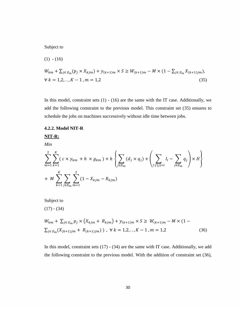
In this model, constraint sets (1) - (16) are the same with the IT case. Additionally, we
add the following constraint to the previous model. This constraint set (35) ensures to
schedule the jobs on machines successively without idle time between jobs.
4.2.2. Model NIT-R
NIT-R:
Min
Subject to
(17) - (34)
(36)
In this model, constraint sets (17) - (34) are the same with IT case. Additionally, we add
the following constraint to the previous model. With the addition of constraint set (36),

31
our model is modified to the version of no idle time between successive jobs is allowed
on machines.
In the next chapter, two different algorithms about the problem are expressed.

32
Chapter 5
Solution Approaches
Models developed in Chapter 4 solve the problems optimally, but due to exponential
time requirements, they are not convenient to use for practical purposes when the
problem size is large. For instance, Model IT is used to solve problem instances with
two-, four- and eight-hour planning horizons including approximately 9, 16, 32 jobs,
respectively. The problems with two-hour data (approximately 9 jobs) take
approximately 1 minute to solve, whereas the four-hour (approximately 16 jobs) data
takes more than 6 hours and the eight-hour (approximately 32 jobs) data could not be
solved with IT model in a reasonable time due to memory problems on a computer with
a 3.7 GHz Intel i7 processor running with a 16 GB of RAM. Although the relaxed model
(IT-R) response is faster than the IT model, it still fails to solve the practical problems in
reasonable time limits. Thus, we propose two computationally efficient heuristic
algorithms: Rolling Horizon Algorithm (RHA) and Two Pass Algorithm (TPA). The aim
of these heuristic algorithms is to schedule the jobs with the lowest inventory level.
These heuristic algorithms split the planning horizon into smaller periods and solve each
period with a proposed exact model. Thus, they can be used to plan for longer horizons
and they also offer the advantage of providing a longer term perspective which allows
flagging potential infeasibility issues in satisfying demand in further periods in time.

33
Note that, as we mentioned in the previous chapter in details, our problem has two
different versions, which are IT and NIT cases. The structure of the heuristics is the
same for both cases, only the corresponding model is different in the heuristics. So, we
explain the proposed algorithm for only one case in this chapter.
In the proposed solution approaches, the general working principle is to divide the
planning horizon into sub-intervals so that each of these sub-intervals can be solved
optimally in a reasonable time by the mathematical models proposed in Chapter 4. In the
following subsections, we provide a description of the general working principles of
these solution approaches.
5. 1. Rolling Horizon Algorithm (RHA)
In this algorithm, first an incumbent planning horizon with a length of t is determined
for which the optimal solution can be found by IT or NIT in a reasonable time. The first
half of the optimal plan obtained for the incumbent horizon is settled as a final plan, and
a new incumbent horizon of length t starting from the ending point of the currently
settled optimal plan is determined. The algorithm proceeds in the same manner and stops
when all of the original planning horizon with length H is exhausted. Let STime and
ETime be the starting and ending time of the planning horizon, respectively and STotal
be the set of jobs in [STime, ETime] time interval. Let t be an interval length where t
ETime – STime (see Figure 5.1-(a)). Firstly, the algorithm takes the first sub-interval and
assumes [STime, STime + t] as the incumbent planning horizon to solve the
corresponding problem optimally with IT-R model. After obtaining the optimal plan for
the incumbent horizon, the algorithm settles the schedule obtained for the first half
[STime, STime + t/2]. In Figure 5.1-(b) the set of jobs that are settled in a final plan is
represented as SSolved. The planning horizon is shown with the blue line. The green line
represents the incumbent planning horizon while the purple line shows the settled plan.
After the first sub-interval is solved, the job list of the planning horizon (STotal) is
updated by subtracting the scheduled jobs. This process actually truncates the original

34
[STime, ETime] with STotal jobs problem into a new problem (STime, ETime) with
SNew = STotal \ SSolved jobs, which is the incumbent job list consisting of the
unscheduled jobs. Since the proposed mathematical model allows the due dates to be
first fulfilled from inventory and later puts back the jobs to inventory, there might be
jobs that are used from inventory in [STime, STime + t/2] and produced in [STime + t/2,
STime + t] time intervals. Note that if we update STime, RHA does not consider these
jobs in the incumbent planning horizon so not updating STime always makes RHA to
reconsider those jobs in the incumbent planning interval. For this reason, the truncated
problem’s time interval starts from STime instead of STime + t/2. This process repeats
by shifting sub-interval t to 3t/2, 2t, 5t/2 … until it reaches to the end of the planning
horizon ETime.
(a)
(b)
Figure 5.1 A representation which shows how Rolling Horizon Algorithm works

35
In the following part, we give the notation that is used throughout the algorithm (see
Table 5.1) and provide the pseudo-code of the algorithm. In the pseudo-code, CTime is
set to STime at the beginning and increased t/2 amount in each iteration. The iterations
continue until STime exceeds the ETime. and are used to feed the
mathematical model so that the model keeps track of the available time of the machine m
and the family of the last job produced, so that it decides when to schedule the job in the
new iteration or to incur a setup time or not. is set to – 1 which corresponds to a
non existing family so that the model incurs a setup time for the first job in the schedule
and and are updated afterwards (see Lines 20 – 22 and 24 – 26,
respectively). At each iteration, the algorithm finds jobs that are in sub-interval [STime,
CTime + t] (see Lines 6 - 8), solves the corresponding optimization problem and then
updates the job list STotal. The model solves the corresponding sub-problem (see Lines
10 – 12) and updates the total job list STotal (see Lines 16 – 18).
Table 5.1 Notations Used in Rolling Horizon Algorithm
Notations
m machine index, m = 1,2
j
t
ETime
STime
job index, j = 1,..,J
length of the interval
ending time of the planning horizon
starting time of the planning horizon
family of job j
most recent setup family on machine m
due date of job j
starting time of job j’s processing operation
Boolean variable showing if the due date for job j is fulfilled from
inventory

36
The machine on which job j is scheduled
set of jobs in (STime, ETime) time interval
list of scheduled jobs where each scheduled job is a tuple
starting time of the operations on each machine m
current time of the system
job set between time x to time y
processing time of a job
Algorithm - RHA Rolling Horizon
1 set to STime
2 set to -1 for each m
3 set to STime
4 while
5
6 for each job
7 if
8 9
10 for each job
11 solve IT-R to obtain , using
12 and
13 SSolved =
14 for each job 15
16 if
17
18 = Stotal \ { j }
19
20 if 1 and = 0 and
21
22 = 23

37
24 if 1 and = 1 and
25
26 =
27
28
The algorithm tries to schedule the jobs in the incumbent planning horizon in line 11 and
in case of infeasibility for the solution in the incumbent planning horizon, the algorithm
increments the contingency stock levels for each family and solves the problem from
scratch. We have not included this procedure to keep the algorithm concise.
5. 2. Two-Pass Algorithm (TPA)
This algorithm has three stages. At the very beginning of this algorithm, the planning
horizon is divided into manageable sub-intervals which can be optimally solved by the
proposed MIP models in a reasonable time. In the first pass stage, the optimal schedules
are found for successive sub-problems by using the proposed IT-R or NIT-R model, also
taking into consideration the last job’s finishing time and the current setup on each
machine. If the finishing time of the last job in a sub-interval exceeds the ending time of
the interval, the excess amount of the processing time on its assigned machine is added
to the starting time of the next sub-interval’s starting time. Continuity between
successive sub-intervals is attained in this way. With this procedure, we find the required
contingency stock and ending inventory level of each sub-interval and compare these
for successive sub-intervals. If ending inventory level of one of the sub-intervals is
different from starting inventory level of the following sub-interval, this will cause a
problem while applying the plans continuously. For that reason, there must be
consistency between the successive sub-intervals’ inventory levels and this is ensured in
the second pass of the algorithm. In the update stage, the job lists of each sub-problem
are updated by comparing the successive sub-problems’ inventory levels. If the
consecutive sub-interval’s ending and contingency stock levels are not equal, the
algorithm deletes the excessive number of jobs from the previous sub-interval’s job list
38
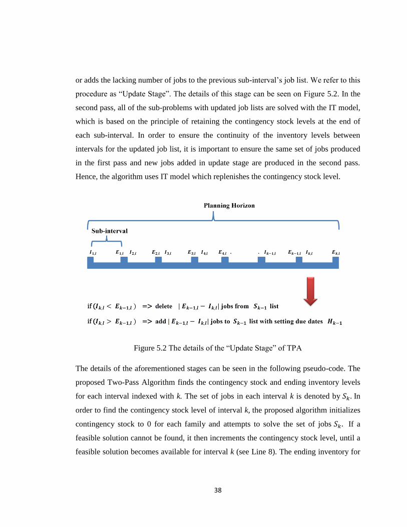
or adds the lacking number of jobs to the previous sub-interval’s job list. We refer to this
procedure as “Update Stage”. The details of this stage can be seen on Figure 5.2. In the
second pass, all of the sub-problems with updated job lists are solved with the IT model,
which is based on the principle of retaining the contingency stock levels at the end of
each sub-interval. In order to ensure the continuity of the inventory levels between
intervals for the updated job list, it is important to ensure the same set of jobs produced
in the first pass and new jobs added in update stage are produced in the second pass.
Hence, the algorithm uses IT model which replenishes the contingency stock level.
Figure 5.2 The details of the “Update Stage” of TPA
The details of the aforementioned stages can be seen in the following pseudo-code. The
proposed Two-Pass Algorithm finds the contingency stock and ending inventory levels
for each interval indexed with k. The set of jobs in each interval k is denoted by In
order to find the contingency stock level of interval k, the proposed algorithm initializes
contingency stock to 0 for each family and attempts to solve the set of jobs If a
feasible solution cannot be found, it then increments the contingency stock level, until a
feasible solution becomes available for interval k (see Line 8). The ending inventory for

39
interval k is calculated by decrementing the contingency stock for the jobs that are used
from the inventory in the computed feasible solution which is done in line 14. In the
update stage, the algorithm provides continuity between the contingency stock and
ending level of intervals. In this stage, the algorithm compares the contingency stock
level of interval k and ending inventory level of interval k – 1. If the contingency stock
level of interval k is less than the ending inventory level of interval k – 1 for some family
l, then the algorithm deletes from the set of jobs which have the earliest due date in
family l and uses it from the inventory (see Line 18). For the other case when the
contingency stock level k is larger than the ending inventory level of k – 1 for some
family l, the algorithm introduces new jobs of family l which have the due date of the
previous interval’s horizon as shown in line 20. Finally, the second pass solves the new
problem with the updated job set for each interval k to ensure the feasibility of the
intervals when new jobs are introduced or existing jobs are removed from the
production. In Line 24, second pass schedules jobs in , in case of infeasibility in that
line, the algorithm increments the contingency stock level at the first interval by
removing jobs according to their due date sequence that are produced in the second pass
and the algorithm starts to the second pass from scratch. This process is not shown in the
pseudo-code to keep the exposition simple.
In addition to the notation in section 5.1 we define the following notations for this
algorithm.
Table 5.2 Notations used in Two-Pass Algorithm
Notations
k interval index, k = 1,..,K
initial inventory requirement of family l at the beginning of the
interval
ending inventory of family l at the end of the interval
set of jobs that must be processed in the interval

40
set of jobs that are used from inventory and not produced in the
interval
solution set that consists of the scheduled jobs at the interval
used from inventory and not produced jobs of family l in the
interval
planning horizon of the interval
Algorithm - TPA Two-Pass
First pass
1 set to STime for each m
2 set to -1 for each m
3 set to
4 for each 5 for each k initialize = 0
6 solve using IT model with and
7 while is infeasible
8 = for all l
9 solve and obtain for all l
10 endwhile
11 compute ) for each l
12 for each
13 if
14 = 15 = + { Update stage
16 for each 17 if 18 delete jobs from list
19 else
20 add jobs with due date to list
Second pass
21 set as the start time of each m
22 for each
23 update by using inventory for each job in
24 solve with and obtained from the first pass using IT
25 model

41
In the next chapter, we first present the test instances and then analyze the solutions
obtained by using the proposed heuristics.

42
Chapter 6
Computational Results
In this chapter, our aim is to show the effectiveness of the heuristic algorithms for the
planning and scheduling problem under study. We compare the heuristics and exact
methods in terms of contingency stock levels, average inventory carrying levels, setup
numbers and CPU times. To this end, we first explain the characteristics of the test
problems and environment we used to compare the heuristics and the exact solution
methods. Afterwards, we give the test results and present their detailed comparisons.
Finally, we summarize the results.
6. 1. Test Instances
We use a test bed which includes both real and random problems. Real problems are
gathered directly from the operations of the body shell department of Oyak-Renault and
the realized demand generated by the consumption line in a specific time period in year
2011. Whereas, random problems are randomly generated with different characteristics
which are appropriate to future goals of the company and suitable to understand the
behavior of the solution methods at different cases.

43
For real problems, data for three consecutive workdays are used to test the heuristic
algorithms and the exact methods. The planning horizon is set to eight hours, therefore
from three work days, we generate nine problem instances since the company is working
for three shifts and 24 hours every day. There are approximately 35 jobs in each
instance. In the current operations of Renault, there are eight different types of doors
demanded by the consumption line, but four of these types are produced by the existing
door manufacturing cells. Therefore, we only include the demand of these four types in
our problem instances. There are seven parameters of the test bed namely, the planning
horizon length, the sub-interval length, the setup times, the processing time, the
inventory holding cost and the setup cost. These parameters can be seen in Table 6.1.
The sub-interval length is used in heuristics. The setup time, holding cost, and setup cost
are given in Table 6.1 by Renault engineers. The processing times depend on the number
of workers allocated to the body shop and assume one of the values given in Table 6.1.
This allocation might change depending on the tactical decisions made by planners.
Hence, we analyze two scenarios for each problem instance, one with a slower operation
(30 vehicles per hour) and the other with a faster operation (20 vehicles per hour). We
denote slow operations by P1 and faster operations by P2.
Table 6.1 The parameters of solution methods for the real problems
Parameters Values
Planning Horizon 28800 sec. (8 hours)
Sub-Interval Length 7200 sec. (2 hours)
Setup Time 300 sec. (5 min.)
Processing Time - 1 960 sec. (16 min.)
Processing Time - 2 1440 sec. (24 min.)
Holding Cost
Setup Cost 3 €
Since Renault aims to increase the flexibility of the manufacturing cells and therefore
the type of the doors manufactured on these cells, we generate the random problems

44
according to their future plans. Thus, in random problems there are six different types of
doors with approximately 30 jobs in total in each instance. For practical purposes, we set
the planning horizon to four hours for random instances.
We employ two different generation methods for the random problems. In the first
generation method GM-S1, there are eight types of doors (which are represented by A,
B, C, D, E, F, G and H) demanded by the consumption line. They are demanded in a
prespecified manner. The details can be seen in Table 6.2. In Table 6.2 where, “Prob.”
represents the probability rate of each type and “Num.” represents the number of jobs of
a given type to be requested consecutively. For instance, in GM-S1, one piece of ‘E’,
‘F’, ‘G’, and ‘H’ door types are demanded and ‘C’ and ‘E’ are demanded twice as many
as them. Likewise, ‘A’ and ‘B’ door types are demanded three times as many ‘D’ and
‘E’. Second generation method GM-S2 is similar to GM-S1 however it has different
probability rates for each type as given in Table 6.2. In order to generate random
problems for a given generation method, we first select a door type among the six
alternatives using a probability distribution for the generation method in Table 6.2 and
place a given number of selected type jobs consecutively (see Table 6.2). The difference
between the due dates of every two consecutive doors demanded by the consumption
line is set as 1 minute and this process is repeated until the time of the last door reaches
to the end of the planning horizon.
Table 6.2 The characteristics of Generation Method
GM
S1 S2
Type Prob. Num. Prob. Num.
A 1/8 6 6/20 6
B 1/8 6 6/20 6
C 1/8 2 2/20 2
D 1/8 2 2/20 2
E 1/8 1 1/20 1
F 1/8 1 1/20 1
G 1/8 1 1/20 1
H 1/8 1 1/20 1
45
The parameters that are used by solution methods are different for the random problems
than real problems. These parameters are listed in Table 6.3. Although the planning
horizon is set to 8 hours in real problems, it is set to 4 hours in random problems because
the number of jobs in random problems is more than that in real problems. The setup
time, holding cost, and setup cost are given the same values that are used in for real
problems as given in Table 6.3. Since the jobs are more frequent in the random problems
than real problems, the company has to work with higher capacity so the processing time
is shorter. However, similar to real problems, there are still two different processing
times, slow (40 vehicles per hour) or fast (60 vehicles per hour). In both test instances,
the parameter M that is used in constraint sets of Model IT and IT-R is set as
which is always greater than the right hand side (RHS) of the
constraints.
Recall that, we have two different versions of the exact methods which are idle time - IT
Model that allows idle time between consecutive jobs and the no idle time - NIT Model
that does not allow such idle time insertion. Throughout the chapter we represent the
solutions with the same abbreviations, so IT represents the solution of the problem
version which allows idle time between jobs and NIT represents the solution of the
problem version which does not allow idle time between consecutive jobs. Besides, we
use P1 (P2) for referring whether the solution is for Processing Time - 1 or Processing
Time - 2. For example, IT-P1 indicates idle time solution with Processing Time -1.

46
Table 6.3 The parameters for random problems
Parameters Values
Planning Horizon 14400 sec. (4 hours)
Sub-Interval Length 7200 sec. (2 hours)
Setup Time 300 sec. (5 min.)
Processing Time - 1 480 sec. (8 min.)
Processing Time - 2 720 sec. (12 min.)
Holding Cost
Setup Cost 3 €
We use JAVA programming language to implement the solution methods and run our
experiments on a computer with a 3.7 GHz Intel i7 processor and 16 GB memory.
6. 2. Computational Results
We solve real and random problems with the heuristic algorithms and exact solution
methods. We present the results of the exact methods in section 6.2.1. We give the
comparison of the exact methods with the heuristics in section 6.2.2. Finally, we
compare the heuristics with each other in section 6.2.3. In the comparisons, we report
average results. The detailed results for each instance of these test problems can be
found in Appendix 1 - 32.
6.2.1. Exact Methods
In this section, we give the results for the exact methods. Note that these methods
attempt to solve test problems with minimum contingency stock levels and increment
them if they cannot find a solution. Additionally, exact solution methods do not allow
decreasing the contingency stock levels in the end of the planning horizon. In Table 6.4,
we show the results for average CPU time and average number of setups for real
problems with the NIT-P2 and IT-P2 exact solutions. We present the results for the
average inventory level and maximum inventory level for each job type among all real
problems in Table 6.5. In general, NIT-P2 solutions have larger average inventory levels

47
than IT-P2 solutions; because in NIT-P2 solutions, idle times between the production of
jobs are not allowed and this leads to compressed production schedule of the demanded
jobs, therefore in the no idle time case, the production of a job starts earlier than that in
the idle time case. This causes carrying more inventories in the no idle time case with
respect to the idle time case. Differently from the solutions for the no idle time case, idle
time solutions shift the production of the jobs forward in the planning horizon as much
as possible. This leads to less number of setups in idle time (IT) solutions. The
maximum inventory level for a job type gives us a good idea about the maximum
number of fully loaded unitizing vessels needed for that type among all problems. The
results can be seen from Table 6.4 and Table 6.5.
Table 6.4 Average CPU time and average number of setups found by exact methods
with the same contingency stock and ending inventory levels for real problems with
processing time 2
Avg. CPU
time (sec.)
Avg. # of Setup
M/C. 1 M/C. 2 Total
P2 NIT 28,164 6.6 4.6 11.1
IT 9,139 6.6 3.2 9.8
Table 6.5 The average and maximum inventory levels obtained by exact methods for
real problems with processing time 2
Exact
Average Inv. Levels Max.Inv.
Type 0 1 2 3 Total 0 1 2 3
P2 NIT 1.01 1.19 1.26 0.79 4.24 4 4 4 3
IT 0.78 0.36 0.64 0.69 2.46 5 2 3 2

48
6.2.2. Comparison of Heuristics with Exact Methods
TPA and RHA are two heuristics we proposed. Unlike the exact methods, TPA and
RHA may decrease the contingency stock levels at the end of the solution. In order to
compare their results with the exact method, we solve the same test instances with the
exact method using the same contingency stock and ending inventory levels that
heuristics found. To this end, we modify Model IT-R (or similarly NIT-R) and refer to
them as IT-R-M (or NIT-R). In the modified model, we change the objective function
for IT-R (or NIT-R) and add the following parameters:
Parameters:
: ending inventory level of family l
: the number of jobs belonging to family l
The details of IT-R-M and NIT-R-M models can be found in the following subsections.
IT-R-M:
Min
Subject to
(17) - (34)
(37)
In this model, constraint sets (17) - (34) are the same as those in the IT - R case
discussed in Chapter 4 and we change the objective function as seen above. With the
addition of constraint set (37), our model is modified so that it finds solutions with given
contingency levels and finishes with given ending inventory levels.

49
NIT-R-M:
Min
Subject to
(17) - (34)
(36)
(38)
In this model, constraint sets (17) - (34) and (36) are the same as that in the NIT - R case
given in Chapter 4 and we change the objective function and add constraint set (38) as
seen above.
6.2.2.1 Comparison of TPA with Exact Methods
We report the results of TPA and exact methods for the real problems in Table 6.6 and
Table 6.7. Table 6.6 shows the average CPU time and average number of setups for each
machine while Table 6.7 lists the average and maximum inventory levels. When we
consider the average running time of the algorithms in Table 6.7-(a), exact methods take
more than 10 hours on the average to solve real problems while TPA solves them in less
than one minute. Obviously, exact methods are not suitable for practical purposes. If we
examine the number of setups, TPA has approximately 10.45 setups on average while
the exact methods have approximately 6.85 setups. TPA schedules the jobs in sub-
intervals and combines them to produce the final schedule, hence it does not consider the
whole planning horizon at once. Therefore, it aims to produce jobs as early so it tends to
carry less inventory than the exact methods. Consequently, the average inventory levels
of TPA are less than the exact methods. Besides, TPA has no higher maximum
inventory levels than exact methods for 14 of 16 different combinations of type,

50
processing time and idle/no idle times factors as seen in Table 6.7-(b). This can explain
one of the reasons for TPA carrying less inventory than exact methods.
Table 6.6 Comparison of average CPU time and average number of setups obtained by
TPA and exact methods for real problems with processing time 1 and 2
Avg. CPU time
(sec.)
Avg. # of Setup
Exact TPA
Exact TPA M/C. 1 M/C. 2 Total M/C. 1 M/C. 2 Total
P1 NIT 47,778 13 4.4 1.9 6.3 6.2 3.0 9.2
IT 36,153 31 4.2 2.3 6.6 7.6 3.1 10.7
P2 NIT 18,385 16 4.8 2.7 7.4 7.2 2.9 10.1
IT 17,538 25 4.6 2.6 7.1 7.3 4.4 11.8
Table 6.7 Comparison of average and maximum inventory levels obtained by TPA and
exact methods for real problems with processing time 1 and 2
Average Inventory Levels
Exact TPA
Type 0 1 2 3 Total 0 1 2 3 Total
P1 NIT 1.74 3.19 1.81 0.70 7.44 1.63 2.48 1.87 0.51 6.49
IT 1.01 1.30 0.89 1.03 4.23 0.54 0.56 0.50 0.60 2.19
P2 NIT 1.16 1.51 1.17 0.60 4.43 1.07 1.56 1.07 0.48 4.19
IT 0.93 0.87 1.07 0.84 3.70 0.84 0.77 0.65 0.81 3.07
(a)
Maximum Inventory Levels
Exact TPA
Type 0 1 2 3 0 1 2 3
P1 NIT 5 7 6 2 6 9 6 2
IT 5 7 5 3 3 3 2 2
P2 NIT 4 5 4 2 3 5 4 2
IT 4 5 5 3 3 5 3 2
(b)

51
We list the results of TPA and exact methods for GM-S1 random problems in Tables 6.8
and 6.9. We present average running time and average number of setups in Table 6.8;
and average and maximum inventory levels in Table 6.9. When we consider the average
CPU time of the algorithms, TPA is quite faster than the exact methods. If we compare
average CPU times of the TPA for random problems with average CPU times of TPA
with real problems, we see that TPA requires more time for random problems than the
real problems. This may indicate relative difficulty of random problems. For the number
of setups, maximum (1.8 setup) and minimum difference (1.1 setup) among average
number of setups indicate that the exact methods are slightly better than the TPA.
Considering the differences between TPA and exact methods in Table 6.6 and 6.8, TPA
is more successful in random problems than it is in real problems with respect to its
number of setups. The data in random problems are uniformly distributed and more
demanding than the real problems; hence this characteristic of the data restricts exact
methods to utilize more empty intervals in the planning horizon. If we examine Table
6.9-(a), TPA has lower average inventory levels than exact methods except GM-S1-NIT-
P2 case. For that case, the exact method has an average inventory level that is 0.1
door/sec. less than TPA’s. In Table 6.9-b, the maximum inventory levels of TPA are less
than those of exact methods for 22 of 24 different combinations of type, processing time
and idle/no idle times factors. The comparison of these combinations shows the
heuristics’ efficiency in terms of the resulting storage area requirements.

52
Table 6.8 Comparison of average CPU time and number of setups obtained by TPA and
exact methods for random problems (GM-S1) with processing time 1 and 2
Avg. CPU time (sec.) Avg. # of Setup
Exact TPA
Exact TPA M/C. 1 M/C. 2 Total M/C. 1 M/C. 2 Total
GM
S1
P1 NIT 20,846 327 3.2 3.0 6.2 4.6 3.0 7.6
IT 25,401 2,256 3.3 3.0 6.3 4.2 3.2 7.4
P2 NIT 38,819 113 3.0 3.0 6.0 4.4 3.0 7.4
IT 49,537 355 3.0 2.4 5.4 4.6 2.6 7.2
Table 6.9 Comparison of average and maximum inventory levels obtained by TPA and
exact methods for random problems (GM-S1) with processing time 1 and 2
Average Inventory Levels
Exact TPA
Type 0 1 2 3 4 5 Total 0 1 2 3 4 5 Total
GM
S1
P1 NIT 2.1 2.7 1.4 1.6 1.2 0.9 10.1 1.9 2.2 1.2 1.0 1.4 1.1 8.8
IT 0.8 1.7 1.4 1.1 0.8 0.7 6.6 1.6 0.7 0.7 0.8 1.0 0.7 5.5
P2 NIT 1.8 1.8 1.4 1.1 1.4 1.2 8.7 2.1 1.6 1.3 1.3 1.3 1.2 8.8
IT 1.2 1.0 0.9 1.4 1.0 0.7 6.1 0.6 0.5 0.8 0.8 1.1 0.8 4.6
(a)
Maximum Inventory Levels
Exact TPA
Type 0 1 2 3 4 5 0 1 2 3 4 5
GM
S1
P1 NIT 7 8 4 4 3 2 6 7 4 3 3 3
IT 5 6 4 3 2 2 5 4 2 2 2 2
P2 NIT 6 5 5 3 3 3 7 5 4 4 3 2
IT 5 5 3 4 2 2 2 2 2 2 2 2
(b)
6.2.2.2 Comparison of RHA and Exact Methods
Similar to TPA, we report the results of RHA and exact methods for real problems in
Tables 6.10 and 6.11. Table 6.10 contains average CPU time and number of setups
information. If we look at the average CPU times in Table 6.10, RHA finds solutions in

53
less than 15 seconds on the average while the exact methods find solutions
approximately in 7 hours. If we compare RHA’s and TPA’s CPU times (Table 6.6) for
real problems, RHA is also faster than TPA, because TPA solves the problem in two
passes. The average number of setups is 7.15 for RHA and 11.05 for the exact methods.
Table 6.11-(a) contains average inventory levels for RHA and exact methods. For the
average inventory levels, RHA is better than the exact methods for the idle time (IT) and
no idle time (NIT) P2 cases, but the exact method is better than RHA for the no idle time
(NIT) P1 case. Maximum inventory levels are given in Table 6.11-(b) and RHA has no
higher maximum inventory levels for 15 of 16 different combinations of type,
processing time and idle/no idle times factors.
Table 6.10 Comparison of CPU time and number of setups obtained by RHA and exact
methods for real problems with processing time 1 and 2 for average
Avg. CPU time (sec.)
Avg. # of Setup
Exact RHA
Exact RHA M/C. 1 M/C. 2 Total M/C. 1 M/C. 2 Total
P1 NIT 48,752 6 4.2 2.2 6.4 10.7 1.6 12.2
IT 27,641 22 4.1 2.3 6.4 7.1 2.0 9.1
P2 NIT 21,852 5 5.4 3.8 9.2 8.6 3.6 12.1
IT 25,143 11 4.3 2.2 6.6 7.6 3.2 10.8
Table 6.11 Comparison of average and maximum inventory levels obtained by RHA and
exact methods for real problems with processing time 1 and 2
Average Inventory Levels
Exact RHA
Type 0 1 2 3 Total 0 1 2 3 Total
P1 NIT 1.82 3.39 2.46 1.15 8.82 2.08 3.72 1.83 0.76 8.40
IT 1.05 0.67 1.12 1.11 3.95 0.64 0.39 0.73 0.35 2.11
P2 NIT 1.17 1.45 1.29 0.73 4.64 1.16 1.97 1.17 0.50 4.80
IT 0.99 0.59 1.03 0.83 3.44 0.72 0.69 0.74 0.57 2.73
(a)

54
Maximum Inventory Levels
Exact RHA
Type 0 1 2 3 0 1 2 3
P1 NIT 5 8 7 3 5 8 4 2
IT 5 7 5 3 3 3 3 2
P2 NIT 4 6 6 3 5 6 4 2
IT 4 4 4 2 4 3 3 2
(b)
We also compare our algorithms with exact methods for random problems as well and
give the results for the GM-S1 cases in Tables 6.12 and 6.13. In terms of CPU times,
RHA is faster than the exact methods for all cases as given in Table 6.12, however its
average setup numbers (approximately 6.75 on average) are greater than the exact
methods (approximately 8.90 on average) for all cases. Average inventory levels for
RHA and exact methods are given in Table 6.13-(a). RHA is better than the exact
methods for all cases except GM-S1-P2 idle time (IT) case. We give results for
maximum inventory levels in Table 6.13-(b). The results indicate that RHA has no
higher maximum inventory levels for 22 of 24 different combinations of type,
processing time and idle/no idle times factors.
Table 6.12 Comparison of average CPU time and number of setups obtained by RHA
and exact methods for random problems (GM-S1) with processing time 1 and 2
Avg. CPU time
(sec.)
Avg. # of Setup
Exact RHA
Exact RHA M/C. 1 M/C. 2 Total M/C. 1 M/C. 2 Total
GM
S1
P1 NIT 19,243 22 3.6 3.2 6.8 4.8 5.0 9.8
IT 42,668 39 3.2 3.0 6.2 4.2 4.2 8.4
P2 NIT 30,386 30 3.8 3.8 7.6 4.4 4.2 8.6
IT 25,194 26 3.6 2.8 6.4 4.4 4.4 8.8
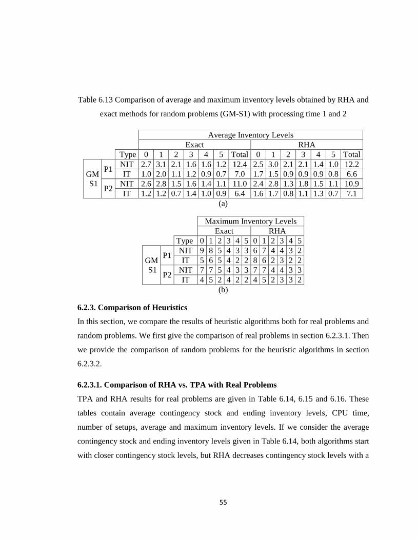
55
Table 6.13 Comparison of average and maximum inventory levels obtained by RHA and
exact methods for random problems (GM-S1) with processing time 1 and 2
Average Inventory Levels
Exact RHA
Type 0 1 2 3 4 5 Total 0 1 2 3 4 5 Total
GM
S1
P1 NIT 2.7 3.1 2.1 1.6 1.6 1.2 12.4 2.5 3.0 2.1 2.1 1.4 1.0 12.2
IT 1.0 2.0 1.1 1.2 0.9 0.7 7.0 1.7 1.5 0.9 0.9 0.9 0.8 6.6
P2 NIT 2.6 2.8 1.5 1.6 1.4 1.1 11.0 2.4 2.8 1.3 1.8 1.5 1.1 10.9
IT 1.2 1.2 0.7 1.4 1.0 0.9 6.4 1.6 1.7 0.8 1.1 1.3 0.7 7.1
(a)
Maximum Inventory Levels
Exact RHA
Type 0 1 2 3 4 5 0 1 2 3 4 5
GM
S1
P1 NIT 9 8 5 4 3 3 6 7 4 4 3 2
IT 5 6 5 4 2 2 8 6 2 3 2 2
P2 NIT 7 7 5 4 3 3 7 7 4 4 3 3
IT 4 5 2 4 2 2 4 5 2 3 3 2
(b)
6.2.3. Comparison of Heuristics
In this section, we compare the results of heuristic algorithms both for real problems and
random problems. We first give the comparison of real problems in section 6.2.3.1. Then
we provide the comparison of random problems for the heuristic algorithms in section
6.2.3.2.
6.2.3.1. Comparison of RHA vs. TPA with Real Problems
TPA and RHA results for real problems are given in Table 6.14, 6.15 and 6.16. These
tables contain average contingency stock and ending inventory levels, CPU time,
number of setups, average and maximum inventory levels. If we consider the average
contingency stock and ending inventory levels given in Table 6.14, both algorithms start
with closer contingency stock levels, but RHA decreases contingency stock levels with a

56
small degree compared to TPA. RHA is faster than TPA in terms of average CPU time
as given in Table 6.15, and TPA has less average number of setups compared to RHA
except P2 idle time (IT) case. The average number of setups are directly oriented with
the number of produced jobs in real problems, so we can say TPA and RHA are similar
to each other in terms of average number of setups although TPA has less average
number of setups in general. The results for the average inventory levels are given in
Table 6.16-(a), RHA has less average inventory levels than TPA for P1 idle time (IT)
and P2 idle time (IT) cases. When we look at the maximum inventory levels at Table
6.16-(b), both algorithms more or less have the same maximum inventory levels, TPA
has no higher maximum inventory levels for 12 of 16 different combinations of type,
processing time and idle/no idle times factors. Similar to TPA, RHA have no higher
maximum inventory levels for 12 of 16 different combinations of type, processing time
and idle/no idle times factors.
Table 6.14 Comparison of average contingency stock and ending inventory levels
obtained by TPA and RHA for real problems with processing time 1 and 2
CS & EI
TPA RHA
CS EI CS EI
Type 0 1 2 3 0 1 2 3 0 1 2 3 0 1 2 3
P1 NIT 1.0 1.0 1.0 1.0 0.0 0.0 0.0 0.0 1.0 1.0 1.0 1.0 1.0 1.0 1.0 0.8
IT 1.0 1.0 1.0 1.0 0.8 0.8 0.8 0.9 1.0 1.0 1.0 1.0 1.0 1.0 1.0 0.9
P2 NIT 1.0 1.6 1.2 1.2 0.1 0.1 0.1 0.1 1.2 1.2 1.2 1.2 0.6 1.0 0.9 0.6
IT 1.3 2.1 1.7 1.3 1.0 1.0 1.0 0.7 1.6 1.6 1.6 1.6 1.1 1.2 0.7 0.4

57
Table 6.15 Comparison of average CPU time and number of setups obtained by TPA
and RHA for real problems with processing time 1 and 2
Avg. CPU
time (sec.)
Avg. # of Setup
TPA RHA
TPA RHA M/C. 1 M/C. 2 Total M/C. 1 M/C. 2 Total
P1 NIT 13 6 6.2 3.0 9.2 10.7 1.6 12.2
IT 31 22 7.6 3.1 10.7 7.1 2.0 9.1
P2 NIT 16 5 7.2 2.9 10.1 8.6 3.6 12.1
IT 25 11 7.3 4.4 11.8 7.6 3.2 10.8
Table 6.16 Comparison of average and maximum inventory levels obtained by
TPA and RHA for real problems with processing time 1 and 2
Average Inventory Levels
TPA RHA
Type 0 1 2 3 Total 0 1 2 3 Total
P1 NIT 1.63 2.48 1.87 0.51 6.49 2.08 3.72 1.83 0.76 8.40
IT 0.54 0.56 0.50 0.60 2.19 0.64 0.39 0.73 0.35 2.11
P2 NIT 1.07 1.56 1.07 0.48 4.19 1.16 1.97 1.17 0.50 4.80
IT 0.84 0.77 0.65 0.81 3.07 0.72 0.69 0.74 0.57 2.73 (a)
Maximum Inventory Levels
TPA RHA
Type 0 1 2 3 0 1 2 3
P1 NIT 6 9 6 2 5 8 4 2
IT 3 3 2 2 3 3 3 2
P2 NIT 3 5 4 2 5 6 4 2
IT 3 5 3 2 4 3 3 2 (b)
6.2.3.2. Comparison of RHA vs. TPA with Random Problems
The results of TPA and RHA for GM-S1 random problems are reported in Table 6.17-
(a) and (b) , 6.18 and 6.19. We give the results for average contingency stock levels and
ending inventory levels in Table 6.17. The results in Table 6.17-(a-b) show that RHA
does not decrease contingency stock levels much compared to TPA. These results are
coherent with the results for real problems in Table 6.15. In Table 6.18, we report results

58
for average CPU time and average number of setups. RHA has CPU time that is less
than one minute in average, but TPA's CPU time average is more than 10 minutes. In
case of average number of setups, RHA plans more setups than TPA, this is normal
since RHA produces more jobs than TPA. We present results for average inventory
levels in Table 6.19-(a) which shows that RHA has higher average inventory levels than
TPA. Since RHA finishes the planning horizon with higher ending inventory levels than
TPA, the results are reasonable. We give the results for maximum inventory levels in
Table 6.19-(b), TPA has less or equal maximum inventory levels than RHA for all cases.
Table 6.17 Comparison of average contingency stock and ending inventory levels
obtained by TPA and RHA for random problems (GM-S1) with processing time 1 and 2
Average CS & EI
TPA
CS EI
Type 0 1 2 3 4 5 0 1 2 3 4 5
P1 NIT 1.6 1.6 1.6 1.6 1.6 1.6 0.0 0.0 0.4 0.4 0.8 0.6
IT 1.6 1.6 1.6 1.6 1.6 1.6 1.0 1.0 1.0 0.8 0.6 0.8
P2 NIT 1.8 1.8 1.8 1.8 1.8 1.8 0.2 0.2 0.6 0.4 0.8 0.8
IT 1.8 1.8 2.0 1.8 1.8 1.8 1.0 1.0 0.4 0.6 0.6 0.8
(a)
Average CS & EI
RHA
CS EI
Type 0 1 2 3 4 5 0 1 2 3 4 5
P1 NIT 1.6 1.6 1.6 1.6 1.6 1.6 1.6 1.6 1.4 1.6 1.2 0.8
IT 1.6 1.6 1.6 1.6 1.6 1.6 1.2 1.6 1.2 1.6 1.2 1.4
P2 NIT 1.8 1.8 1.8 1.8 1.8 1.8 1.8 1.8 1.4 1.4 1.6 1.2
IT 1.8 1.8 1.8 1.8 1.8 1.8 1.6 1.6 1.0 1.8 1.2 1.0
(b)

59
Table 6.18 Comparison of TPA vs. RHA for random problems (GM-S1) with processing
time 1 & 2 for average CPU time and number of setups
Avg. CPU time (sec.)
Avg. # of Setup
TPA RHA
TPA RHA M/C. 1 M/C. 2 Total M/C. 1 M/C. 2 Total
GM
S1
P1 NIT 327 22 4.6 3.0 7.6 4.8 5.0 9.8
IT 2,256 39 4.2 3.2 7.4 4.2 4.2 8.4
P2 NIT 113 30 4.4 3.0 7.4 4.4 4.2 8.6
IT 355 26 4.6 2.6 7.2 4.4 4.4 8.8
Table 6.19 Comparison of average and maximum of maximum inventory levels obtained
by TPA and RHA for random problems (GM-S1) with processing time 1 and 2
Average Inventory Levels
TPA RHA
Type 0 1 2 3 4 5 Total 0 1 2 3 4 5 Total
GM
S1
P1 NIT 1.9 2.2 1.2 1.0 1.4 1.1 8.8 2.5 3.0 2.1 2.1 1.4 1.0 12.2
IT 1.6 0.7 0.7 0.8 1.0 0.7 5.5 1.7 1.5 0.9 0.9 0.9 0.8 6.6
P2 NIT 2.1 1.6 1.3 1.3 1.3 1.2 8.8 2.4 2.8 1.3 1.8 1.5 1.1 10.9
IT 0.6 0.5 0.8 0.8 1.1 0.8 4.6 1.6 1.7 0.8 1.1 1.3 0.7 7.1
(a)
Maximum Inventory Levels
TPA RHA
Type 0 1 2 3 4 5 0 1 2 3 4 5
GM S1
P1 NIT 6 7 4 3 3 3 6 7 4 4 3 2
IT 5 4 2 2 2 2 8 6 2 3 2 2
P2 NIT 7 5 4 4 3 2 7 7 4 4 3 3
IT 2 2 2 2 2 2 4 5 2 3 3 2
(b)
The results for TPA and RHA for GM-S2 random problems are reported in Table 6.20,
6.21, 6.22. In Table 6.20, we report average contingency stock and ending inventory
levels in Table 6.20. The results show that although TPA and RHA start from the same
average contingency stock, TPA consumes the contingency stock levels more than RHA
does. If we look at the average CPU time and number of setups comparison of TPA and

60
RHA in Table 6.21, TPA is slower than RHA in terms of average CPU time, and it
schedules less number of setups than RHA. We give results for average and maximum
inventory levels in Table 6.22. Since TPA decreases the ending inventory levels, it has
less average inventory than the RHA as given in Table 6.22-(a). Results for the
maximum inventory levels in Table 6.22-(b) indicate that TPA has less or equal
maximum inventory levels than RHA for 21 of 24 different combinations of type,
processing time and idle/no idle times factors. This can be explained also with the
decreased contingency stock levels in TPA.
Table 6.20 Comparison of average contingency stock & ending inventory levels
obtained by TPA and RHA for random problems (GM-S2) with processing time 1 and 2
CS & EI
TPA
CS EI
Type 0 1 2 3 4 5 0 1 2 3 4 5
GM-1 S2
P1 NIT 1.0 1.0 1.0 1.0 1.0 1.0 0.0 0.2 0.0 0.0 0.0 0.0
IT 1.0 1.0 1.0 1.0 1.0 1.0 0.6 0.6 0.4 0.6 0.6 0.6
P2 NIT 1.8 1.8 1.8 1.8 1.8 1.8 0.4 0.6 0.2 0.4 0.2 0.0
IT 1.8 1.8 1.8 1.8 1.8 1.8 1.0 1.2 1.0 1.0 1.0 1.0
(a)
CS & EI
RHA
CS EI
Type 0 1 2 3 4 5 0 1 2 3 4 5
GM-1 S2
P1 NIT 1.0 1.0 1.0 1.0 1.0 1.0 1.0 1.0 1.0 1.0 1.0 1.0
IT 1.0 1.0 1.0 1.0 1.0 1.0 1.0 0.8 1.0 1.0 1.0 1.0
P2 NIT 1.8 1.8 1.8 1.8 1.8 1.8 1.8 1.8 1.8 1.8 1.6 1.6
IT 1.8 1.8 1.8 1.8 1.8 1.8 1.8 1.8 1.8 1.8 1.8 1.6
(b)

61
Table 6.21 Comparison of average CPU time and number of setups obtained by
TPA and RHA for random problems (GM-S2) with processing time 1 and 2
Avg. CPU time (sec.) Avg. # of Setup
TPA RHA
TPA RHA M/C. 1 M/C. 2 Total M/C. 1 M/C. 2 Total
GM
S2
P1 NIT 40 18 4.2 4.2 8.4 5.8 5.0 10.8
IT 257 32 4.8 4.6 9.4 5.4 4.2 9.6
P2 NIT 30 15 4.4 2.8 7.2 5.4 4.6 10.0
IT 116 17 4.4 4.2 8.6 4.2 4.6 8.8
Table 6.22 Comparison of TPA vs. RHA for random problems (GM-S2) with processing
time 1 & 2 for average and maximum inventory levels
Average Inventory Levels
TPA RHA
Type 0 1 2 3 4 5 Total 0 1 2 3 4 5 Total
GM
S2
P1 NIT 0.9 1.1 1.2 1.4 1.1 0.9 6.6 1.5 1.4 1.7 2.0 1.7 1.5 9.9
IT 0.5 0.7 0.7 0.5 0.5 0.5 3.3 0.7 0.5 0.7 0.6 0.7 0.5 3.8
P2 NIT 1.2 1.4 1.4 1.6 1.6 1.0 8.2 2.0 1.9 2.2 2.0 1.8 1.9 11.8
IT 1.1 1.0 0.9 0.8 0.7 0.7 5.2 1.7 1.4 1.4 1.1 0.8 1.5 7.8
(a)
Maximum Inventory Levels
TPA RHA
Type 0 1 2 3 4 5 0 1 2 3 4 5
GM S2
P1 NIT 3 4 5 4 5 4 4 4 4 5 5 4
IT 2 3 3 2 2 2 2 3 2 3 3 2
P2 NIT 3 4 5 5 5 4 4 3 5 5 5 4
IT 2 2 2 2 2 3 5 4 4 3 3 4
(b)
6.3. Summary
Exact methods are better than the heuristics, they optimize number of setups and average
inventory levels. However, they are impractical because of their CPU time and it is not
convenient to use them. The heuristics generally have better or close average inventory
levels compared to exact methods, this is important due to the storage area restrictions.
We decrease approximately 70% of the current inventory levels in the company. As we

62
mentioned before, maximum inventory levels are also important when we consider the
number of unitizing vessels. Our heuristic algorithms decreased the current maximum
inventory levels of the company by about 75%. RHA and TPA obtain their best results
for the random data case, which is appropriate for the near future goal of the company in
which they want to increment the number of door types and want to solve scheduling
problems with more frequent demand of jobs as simulated in random problems.
Additionally, our algorithms are flexible such that they adapt to cases of infeasibility and
they always give the best solution they can find by starting from the lowest minimal
contingency stock and incrementing until they have a feasible solution. This is also
important for practical purposes. When we compare RHA and TPA, we see that RHA
conserves contingency stock levels better than TPA and it is faster than TPA. In terms of
average and maximum inventory levels and number of setups, TPA is better than RHA.
Renault company can use either of the solutions according to their purposes.

63
Chapter 7
Conclusion & Future Directions
This thesis proposes two mixed integer programming based solution approaches to make
integrated inventory carrying and scheduling decisions in a parallel machine
environment subject to machine eligibility restrictions.
Both heuristics provide effective results and are computationally efficient for practical
purposes. The algorithms are general enough to be of value to other plants or
departments and applications that involve the use of robotic/flexible manufacturing cells
feeding a downstream operation with a steady demand pattern. Both algorithms (RHA
and TPA) are programmed in Java programming language using the Gurobi library. We
obtain solutions that synchronize the operations in the door manufacturing processes
with the speed of the consumption line. In this way, we obtain significant reductions in
the inventory levels with respect to the current levels. In comparison to the exact
methods, the two algorithms have significantly modest CPU time requirements. Still,
they lead to a reduction of about 70% in the present inventory levels at Oyak-Renault.
These results and other potential benefits offered by our solution approaches to the
company are verified and validated based on real data collected at real and random

64
problems test scenarios. Renault engineers and planners also attest to the practical
applicability of the resulting production plans. Currently, the algorithms proposed in this
thesis are being implemented at Renault in the form a decision support system and pilot
studies are expected to commence in the end of 2012.
One future research direction is to investigate other heuristic mechanisms to better
capture the trade-offs between doing setup or keeping inventory. Additionally, design of
the solutions for multiple machines and different shop structures is another direction that
can increase the generality of possible applications.

65
Bibliography
Allahverdi, A., Gupta J.N.D., and Aldowaisan T. "A review of scheduling research
involving setup considerations." OMEGA The International Journal of Management
Sciences, 1999: 219–239.
Allahverdi, A., Ng C., Cheng T., and Kovalyov M. "A survey of scheduling problems
with setup times or costs." European Journal of Operational Research, 2008: 985-1032.
Azizoglu, M., and Webster S. "Scheduling parallel machines to minimize weighted
flowtime with family set-up times." International Journal of Production Research,
2003: 1199-1215.
Bir´o, P., and McDermid E. "Matching with sizes (or scheduling with processing set
restrictions)." Discrete Applied Mathematics, 2011.
Brucker, P., Kovalyov M.Y., Shafransky Y.M., and F. Werner. "Batch scheduling with
deadlines on parallel machines." Annals of Operations Research, 1998: 23-40.
Centeno, G., and Armacost R.L. "Minimizing makespan on parallel machines with
release time and machine eligibility restrictions." International Journal of Production
Research, 2004: 1243-1256.
Centeno, G., and Armacost R.L. "Parallel machine scheduling with release time and
machine eligibility restrictions." Computers & Industrial Engineering, 1997: 273-276.
Chen, J.F., and Wu T.H. "Total tardiness minimization on unrelated parallel machine
scheduling with auxiliary equipment constraints." Omega, 2006: 81-89.
Chen, Z.L., and Powell W.B. "Exact algorithms for scheduling multiple families of jobs
on parallel machines." Naval Research Logistics (NRL), 2003: 823-840.

66
Cheng, T.C.E., and Chen Z.L. "Parallel machine scheduling with batch setup times."
Operations Research, 1994: 1171-1174.
Dunstall, S., and Wirth A. "A comparison of branch-and-bound algorithms for a family
scheduling problem with identical parallel machines." European Journal of Operational
Research, 2005a: 283-296.
Dunstall, S., and Wirth A. "Heuristic methods for the identical parallel machine
flowtime problem with set-up times." Computers & Operations Research, 2005b: 2479-
2491.
Epstein, L., and Levin A. "Scheduling with processing set restrictions: PTAS results for
several variants." International Journal of Production Economics, 2011: 586-595.
Gambosi, G., and Nicosia G. "On-line scheduling with setup costs." Information
Processing Letters, 2000: 61-68.
Glass, C.A., and Mills H.R. "Scheduling unit length jobs with parallel nested machine
processing set restrictions." Computers & Operations Research, 2006: 620-638.
Huo, Y., and Leung J.Y.T. "Fast approximation algorithms for job scheduling with
processing set restrictions." Theoretical Computer Science, 2010b: 3947-3955.
Huo, Y., and Leung J.Y.T. "Parallel machine scheduling with nested processing set
restrictions." European Journal of Operational Research, 2010a: 229-236.
Lawler, E. L., Lenstra J. K., Rinnooy Kan A.H.G., and Shmoys D.B. "Sequencing and
scheduling: Algorithms and complexity." Handbooks in Operations Research and
Management Science, 1993: 445-522.
Lee, K., Leung J., and M. Pinedo. "Makespan minimization in online scheduling with
machine eligibility." 4OR: A Quarterly Journal of Operations Research, 2010: 331-364.
Lee, K., Leung J.Y.T., and M. Pinedo. "Scheduling jobs with equal processing times
sucject to machine eligibility constraints." Journal of Scheduling, 2011: 27-38.
Leung, J.Y.T., Ng C.T., and Cheng T.C.E. "Minimizing sum of completion times for
batch scheduling of jobs with deteriorating processing times." European Journal of
Operational Research, 2008: 1090-1099.

67
Leung, J.Y.Y., and Li C.L. "Scheduling with processing set restrictions: A survey."
International Journal of Production Economics, 2008: 251-262.
Li, C.L. "Scheduling unit-length jobs with machine eligibility restrictions." European
Journal of Operational Research, 2006: 1325-1328.
Liaee, M., and Emmons H. "Scheduling families of jobs with setup times." International
Journal of Production Economics, 1997: 165-176.
Liao, C. J., Chao C.W., and Chen L.C. "An improved heuristic for parallel machine
weighted flowtime scheduling with family set-up times." Computers & Mathematics
with Applications, 2012: 110-117.
Lin, B.M.T., and Jeng A.A.K. "Parallel-machine batch scheduling to minimize the
maximum lateness and the number of tardy jobs." International Journal of Production
Economics, 2004: 121-134.
Lin, Y., and Li W. "Parallel machine scheduling of machine-dependent jobs with unit-
length." European Journal of Operational Research, 2004: 261-266.
Liu, Z., Yu W., and Cheng T.C. "Scheduling groups of unit length jobs on two identical
parallel machines." Information Processing Letters, 1999: 275-281.
Monma, C.L., and Potts C.N. "Analysis of heuristics for preemptive parallel machine
scheduling with batch setup times." Operations Research, 1993: 981-993.
Monma, C.L., and Potts C.N. "On the complexity of scheduling with batch setup times."
Operations Research, 1989: 798-804.
Ou, J., Leung J., and Li C.L. "Scheduling parallel machines with inclusive processing set
restrictions." Naval Research Logistics (NRL), 2008: 328-338.
Pinedo, M. Scheduling: Theory, Algorithms, and Systems. Springer Verlag, 1995.
Potts, C.N., and Kovalyov M.Y. "Scheduling with batching: a review." European
Journal of Operational Research, 2000: 228-249.
Schutten, J.M.J., and Leussink R.A.M. "Parallel machine scheduling with release dates,
due dates and family setup times." International Journal of Production Economics,
1996: 119-125.

68
So, K.C. "Some heuristics for scheduling jobs on parallel machines with setups."
Management Science, 1990: 467-475.
Tang, C.S. "Scheduling batches on parallel machines with major and minor set-ups."
European Journal of Operational Research, 1990: 28-37.
Tang, C.S., and Wittrock R.J. "Parallel machine scheduling with major and minor
setups." International Journal of Flexible Manufacturing Systems, 1985.
Webster, S., and Azizoglu M. "Dynamic programming algorithms for scheduling
parallel machines with family setup times." Computers & Operations Research, 2001:
127-137.
Wilson, A.D., King R.E., and Hodgson T.J. "Scheduling non-similar groups on a flow
line: multiple group setups." Robotics and Computer-Integrated Manufacturing, 2004:
505-515.
Wittrock, R.J. "Scheduling parallel machines with major and minor setup times."
International Journal of Flexible Manufacturing Systems, 1990: 329-341.
Yang, W.H. "Scheduling two-component products on parallel machines." Omega, 2004:
353-359.
Yi, Y., and Wang D.W. "Soft computing for scheduling with batch setup times and
earliness-tardiness penalties on parallel machines." Journal of Intelligent Manufacturing,
2003: 311-322.
Yi, Y., Chang H.Y., Wang J., and Bai J.C. "Soft computing for parallel scheduling with
setup times." Machine Learning and Cybernetics, 2004. Proceedings of 2004
International Conference on. IEEE, 2004. 2041-2046.

69
APPENDIX

70
CPU Time # of Setup Average Mean and Max. Inventory Levels CS EI
Type 0 Type 1 Type 2 Type 3
Total Type Type
Day Shift (sec.) M/C. 1 M/C. 2 Total Mean Max Mean Max Mean Max Mean Max 0 1 2 3 0 1 2 3
P2
NIT
1
1 16,701 5 5 10 0.88 3 1.05 3 1.39 4 1.19 3 4.5 1 1 1 1 1 1 1 1
2 50,164 5 3 8 0.86 3 1.61 4 1.47 3 1.16 2 5.1 1 1 1 1 1 1 1 1
3 15,839 8 4 12 0.72 2 1.67 4 1.11 3 0.73 2 4.2 1 1 1 1 1 1 1 1
2
1 36,896 10 5 15 1.09 3 1.23 3 0.76 2 0.23 1 3.3 1 1 1 1 1 1 1 1
2 65,771 7 6 13 0.69 2 0.75 2 1.52 4 0.40 1 3.4 1 1 1 1 1 1 1 1
3 15,353 6 4 10 1.49 3 1.05 3 1.01 3 0.63 2 4.2 1 1 1 1 1 1 1 1
3
1 27,452 10 6 16 0.44 2 0.96 2 0.70 2 0.51 1 2.6 1 1 1 1 1 1 1 1
2 18,686 4 4 8 1.81 4 1.05 3 1.63 4 1.19 3 5.7 1 1 1 1 1 1 1 1
3 6,620 4 4 8 1.13 3 1.31 3 1.71 4 1.06 2 5.2 1 1 1 1 1 1 1 1
Average. 28,165 6.6 4.6 11.1 1.0
1.2
1.3
0.8
4.2
IT
1
1 13,024 6 3 9 0.56 2 0.30 2 0.61 2 0.72 2 2.2 1 1 1 1 1 1 1 1
2 48,151 5 3 8 0.60 2 0.42 2 0.64 2 0.74 2 2.4 1 1 1 1 1 1 1 1
3 2,416 6 3 9 0.65 2 0.22 1 0.67 3 1.03 2 2.6 1 1 1 1 1 1 1 1
2
1 1,885 8 3 11 0.57 2 0.49 2 0.83 3 0.26 1 2.1 1 1 1 1 1 1 1 1
2 5,913 9 3 12 0.74 2 0.44 2 0.56 2 0.42 2 2.2 1 1 1 1 1 1 1 1
3 2,621 6 3 9 0.54 2 0.35 2 0.90 3 0.81 2 2.6 1 1 1 1 1 1 1 1
3
1 1,650 10 5 15 0.38 2 0.30 2 0.48 2 0.43 1 1.6 1 1 1 1 1 1 1 1
2 2,016 4 3 7 2.15 5 0.25 2 0.46 2 0.88 2 3.7 1 1 1 1 1 1 1 1
3 4,584 5 3 8 0.80 3 0.45 2 0.60 2 0.89 2 2.7 1 1 1 1 1 1 1 1
Average. 9,140 6.6 3.2 9.8 0.8
0.4
0.6
0.7
2.5
Appendix 1 The solutions found by exact methods with the same contingency stock and ending inventory levels for real problems with processing time 2 based on CPU
time and number of setups

71
CPU Time # of Setup
(sec.) Exact TPA
Day Shift Exact TPA M/C. 1 M/C. 2 Total M/C. 1 M/C. 2 Total
P1
NIT
1
1 14,389 7 5 1 6 3 5 8
2 23,798 12 5 1 6 11 1 12
3 164,957 12 5 2 7 4 5 9
2
1 3,831 12 4 2 6 3 5 8
2 66,569 19 4 2 6 6 2 8
3 81,489 21 5 2 7 7 1 8
3
1 4,966 16 4 3 7 3 5 8
2 47,390 9 4 2 6 10 1 11
3 22,607 9 4 2 6 9 2 11
Average 47,777 13 4 2 6 6 3 9
IT
1
1 3,075 18 4 2 6 7 3 10
2 32,659 22 4 1 5 6 3 9
3 72711 25 4 2 6 6 4 10
2
1 7,539 37 5 2 7 8 3 11
2 95,425 34 5 2 7 10 2 12
3 39,631 41 4 3 7 8 3 11
3
1 18,184 40 5 3 8 8 4 12
2 32,235 37 4 3 7 9 2 11
3 23,916 22 3 3 6 6 4 10
Average 36,153 31 4 2 7 8 3 11
Appendix 2 1 Comparison of CPU time and number of setups obtained by TPA and exact methods for real problems with processing time 1

72
CPU Time # of Setup
(sec.) Exact TPA
Day Shift Exact TPA M/C. 1 M/C. 2 Total M/C. 1 M/C. 2 Total
P2
NIT
1
1 19,950 6 6 2 8 7 2 9
2 25,849 14 4 3 7 6 4 10
3 4,447 9 6 3 9 9 2 11
2
1 40,469 7 5 2 7 7 2 9
2 31,512 19 5 2 7 5 4 9
3 3,132 17 4 2 6 6 4 10
3
1 11,174 39 4 3 7 8 2 10
2 9,068 9 5 3 8 8 2 10
3 19,859 18 4 4 8 9 4 13
Average 18,384 15 5 3 7 7 3 10
IT
1
1 23,013 14 6 2 8 7 4 11
2 33,381 15 4 3 7 7 5 12
3 14,188 18 4 3 7 8 4 12
2
1 17,693 18 6 2 8 8 6 14
2 11,217 15 4 3 7 9 4 13
3 22,241 102 3 2 5 6 3 9
3
1 13,285 15 4 2 6 8 4 12
2 9,068 8 5 3 8 5 4 9
3 13,753 15 5 3 8 8 6 14
Average 17,538 25 5 3 7 7 4 12
Appendix 3 2 Comparison of CPU time and number of setups obtained by TPA and exact methods for real problems with processing time 2

73
CS & EI
Exact TPA
CS (Type) EI (Type) CS (Type) EI (Type)
Day Shift 0 1 2 3 0 1 2 3 0 1 2 3 0 1 2 3
P1
NIT
1
1 1 1 1 1 0 0 0 0 1 1 1 1 0 0 0 0
2 1 1 1 1 0 0 0 0 1 1 1 1 0 0 0 0
3 1 1 1 1 0 0 0 0 1 1 1 1 0 0 0 0
2
1 1 1 1 1 0 0 0 0 1 1 1 1 0 0 0 0
2 1 1 1 1 0 0 0 0 1 1 1 1 0 0 0 0
3 1 1 1 1 0 0 0 0 1 1 1 1 0 0 0 0
3
1 1 1 1 1 0 0 0 0 1 1 1 1 0 0 0 0
2 1 1 1 1 0 0 0 0 1 1 1 1 0 0 0 0
3 1 1 1 1 0 0 0 0 1 1 1 1 0 0 0 0
Average 1.00 1.00 1.00 1.00 0.00 0.00 0.00 0.00 1.00 1.00 1.00 1.00 0.00 0.00 0.00 0.00
IT
1
1 1 1 1 1 1 1 1 1 1 1 1 1 1 1 1 1
2 1 1 1 1 1 1 1 1 1 1 1 1 1 1 1 1
3 1 1 1 1 0 0 0 1 1 1 1 1 0 0 0 1
2
1 1 1 1 1 1 1 1 1 1 1 1 1 1 1 1 1
2 1 1 1 1 0 0 0 0 1 1 1 1 0 0 0 0
3 1 1 1 1 1 1 1 1 1 1 1 1 1 1 1 1
3
1 1 1 1 1 1 1 1 1 1 1 1 1 1 1 1 1
2 1 1 1 1 1 1 1 1 1 1 1 1 1 1 1 1
3 1 1 1 1 1 1 1 1 1 1 1 1 1 1 1 1
Average 1.00 1.00 1.00 1.00 0.78 0.78 0.78 0.89 1.00 1.00 1.00 1.00 0.78 0.78 0.78 0.89
Appendix 4 Comparison of contingency stock & ending inventory levels obtained by TPA and exact methods for real prolems with processing time 1

74
CS & EI
Exact TPA
CS (Type) EI (Type) CS (Type) EI (Type)
Day Shift 0 1 2 3 0 1 2 3 0 1 2 3 0 1 2 3
P2
NIT
1
1 1 1 1 2 0 0 0 0 1 1 1 2 0 0 0 0
2 1 2 1 1 0 0 0 0 1 2 1 1 0 0 0 0
3 1 1 1 1 0 0 0 0 1 1 1 1 0 0 0 0
2
1 1 2 2 1 0 0 0 0 1 2 2 1 0 0 0 0
2 1 2 2 1 0 0 0 0 1 2 2 1 0 0 0 0
3 1 2 1 1 0 0 0 0 1 2 1 1 0 0 0 0
3
1 1 2 1 2 0 0 0 0 1 2 1 2 0 0 0 0
2 1 1 1 1 1 1 1 0 1 1 1 1 0 0 0 0
3 1 1 1 1 1 1 1 1 1 1 1 1 1 1 1 1
Average 1.00 1.56 1.22 1.22 0.22 0.22 0.22 0.11 1.00 1.56 1.22 1.22 0.11 0.11 0.11 0.11
IT
1
1 1 1 1 2 1 1 1 1 1 1 1 2 1 1 1 1
2 1 2 1 1 1 1 1 1 1 2 1 1 1 1 1 1
3 1 2 2 1 1 1 1 0 1 2 2 1 1 1 1 0
2
1 1 2 2 1 1 1 1 1 1 2 2 1 1 1 1 1
2 1 2 2 1 1 1 1 0 1 2 2 1 1 1 1 0
3 3 5 3 2 1 1 1 1 3 5 3 2 1 1 1 1
3
1 2 3 2 2 1 1 1 1 2 3 2 2 1 1 1 1
2 1 1 1 1 1 1 1 0 1 1 1 1 1 1 1 0
3 1 1 1 1 1 1 1 1 1 1 1 1 1 1 1 1
Average 1.33 2.11 1.67 1.33 1.00 1.00 1.00 0.67 1.33 2.11 1.67 1.33 1.00 1.00 1.00 0.67
Appendix 5 Comparison of contingency stock & ending inventory levels obtained by TPA and exact methods for real prolems with processing time 2

75
Average Mean and Max. Inventory Levels
Exact TPA
Type 0 Type 1 Type 2 Type 3 Total
Type 0 Type 1 Type 2 Type 3 Total
Day Shift Mn. Mx. Mn. Mx. Mn. Mx. Mn. Mx. Mn. Mx. Mn. Mx. Mn. Mx. Mn. Mx.
P1
NIT
1
1 1.46 4 3.71 7 1.41 4 0.60 2 7.18 1.12 3 2.26 5 2.43 5 0.69 2 6.49
2 1.49 4 3.78 7 1.16 3 1.09 2 7.52 0.59 2 4.58 9 0.88 3 0.26 1 6.31
3 2.36 5 2.95 6 1.45 4 0.81 2 7.57 1.52 4 1.88 4 2.86 6 0.71 2 6.97
2
1 1.16 3 3.80 7 1.84 4 0.52 2 7.33 1.21 3 1.98 4 2.48 5 0.68 2 6.35
2 1.64 4 2.91 7 2.56 6 0.40 1 7.51 1.51 3 3.27 7 2.12 4 0.45 1 7.35
3 1.99 4 3.74 7 1.53 4 0.60 2 7.87 1.75 4 3.74 7 1.56 4 0.52 1 7.57
3
1 2.41 5 2.15 5 1.59 4 0.51 2 6.66 1.03 3 1.87 4 2.43 5 0.60 2 5.92
2 1.88 4 3.07 6 2.06 4 0.78 2 7.79 3.12 6 1.02 3 1.19 4 0.30 1 5.64
3 1.29 3 2.59 6 2.72 6 0.94 2 7.53 2.81 6 1.70 5 0.92 3 0.37 1 5.81
Average 1.74
3.19
1.81
0.70
7.44 1.63
2.48
1.87
0.51
6.49
IT
1
1 0.32 2 2.95 7 0.76 3 1.09 3 5.11 0.68 2 0.56 2 0.55 2 0.68 2 2.46
2 2.38 5 1.07 4 0.74 3 0.93 2 5.13 0.52 2 0.61 2 0.78 2 0.70 2 2.62
3 1.70 4 1.19 4 0.62 2 0.95 2 4.46 0.41 2 0.77 2 0.49 2 0.80 2 2.46
2
1 0.58 3 2.35 5 1.59 4 1.09 2 5.62 0.61 2 0.66 2 0.74 2 0.80 2 2.81
2 1.46 4 0.16 2 0.27 2 0.39 1 2.28 0.34 2 0.22 2 0.34 2 0.16 1 1.05
3 0.67 3 2.71 6 0.52 2 1.22 3 5.11 0.66 3 0.48 3 0.38 2 0.38 1 1.90
3
1 0.87 3 0.29 2 0.67 3 1.26 3 3.09 0.41 2 0.59 2 0.37 1 0.72 2 2.09
2 1.01 3 0.19 2 1.24 4 0.51 2 2.95 0.72 2 0.45 2 0.47 2 0.40 2 2.03
3 0.12 1 0.75 3 1.59 5 1.80 3 4.27 0.49 2 0.70 2 0.36 2 0.73 2 2.28
Average 1.01
1.30
0.89
1.03
4.23 0.54
0.56
0.50
0.60
2.19
Appendix 6 Comparison of average mean and max. inventory levels obtained by TPA and exact methods for real prolems with processing time 1

76
Average Mean and Max. Inventory Levels
Exact TPA
Type 0 Type 1 Type 2 Type 3 Total
Type 0 Type 1 Type 2 Type 3 Total
Day Shift Mn. Mx. Mn. Mx. Mn. Mx. Mn. Mx. Mn. Mx. Mn. Mx. Mn. Mx. Mn. Mx.
P2
NIT
1
1 1.16 3 1.40 3 0.96 3 0.59 2 4.11 1.33 3 0.70 2 1.02 3 0.59 2 3.65
2 1.47 4 1.20 3 1.36 3 0.81 2 4.84 1.09 2 1.91 4 1.21 3 0.46 1 4.67
3 0.71 2 1.53 3 1.08 3 0.51 1 3.83 0.98 3 1.28 3 1.07 3 0.16 1 3.49
2
1 1.38 3 1.62 4 1.00 2 0.80 2 4.79 0.98 2 2.22 5 0.87 2 0.46 1 4.54
2 1.44 3 1.76 4 1.31 3 0.45 1 4.96 1.11 3 1.06 3 1.88 4 0.56 1 4.60
3 1.45 4 1.56 4 1.18 3 0.51 2 4.70 0.83 2 1.50 4 1.28 3 0.54 1 4.15
3
1 1.18 3 1.35 3 1.51 4 0.38 2 4.42 1.18 3 1.23 3 0.68 2 0.57 2 3.65
2 0.49 2 1.84 5 0.40 2 0.27 1 8.23 1.00 3 2.23 5 0.82 3 0.18 1 8.23
3 1.13 3 1.31 3 1.71 4 1.06 2 5.21 1.15 3 1.92 5 0.82 2 0.82 2 4.71
Average 1.16
1.51
1.17
0.60
5.01 1.07
1.56
1.07
0.48
4.63
IT
1
1 0.61 2 2.16 5 0.88 3 0.41 2 4.06 0.71 2 0.61 2 0.53 2 0.92 2 2.77
2 0.98 3 0.72 2 2.19 5 0.61 2 4.50 0.56 2 0.85 2 0.38 1 0.72 2 2.52
3 0.73 2 0.99 3 0.51 2 0.80 2 3.04 0.92 2 0.64 3 0.76 2 0.60 1 2.92
2
1 1.16 3 0.26 2 0.74 2 1.24 3 3.39 0.55 2 0.56 2 0.83 2 0.87 2 2.81
2 1.43 4 0.27 2 0.72 3 0.97 2 3.40 0.58 2 0.46 2 0.82 2 0.58 1 2.44
3 1.41 3 0.83 5 1.96 4 0.57 2 4.76 1.72 3 1.41 5 1.01 3 1.01 2 5.14
3
1 0.76 2 0.27 3 1.61 4 1.78 3 4.42 1.10 3 1.07 3 0.63 2 1.18 2 3.97
2 0.49 2 1.84 5 0.40 2 0.27 1 3.00 0.70 2 0.82 2 0.52 2 0.62 2 2.65
3 0.80 3 0.45 2 0.60 2 0.89 2 2.73 0.75 2 0.54 2 0.39 2 0.75 2 2.42
Average 0.93
0.87
1.07
0.84
3.70 0.84
0.77
0.65
0.81
3.07
Appendix 7 Comparison of average mean and max. inventory levels obtained by TPA and exact methods for real prolems with processing time 2

77
# of Setup
CPU Time sec. Exact TPA
Day Exact TPA M/C. 1 M/C. 2 Total M/C. 1 M/C. 2 Total
S1
P1
NIT
1 5,773 199 4 3 7 3 5 8
2 6,946 42 2 4 6 6 1 7
3 23,625 686 3 3 6 4 3 7
4 50,119 664 3 3 6 5 3 8
5 17,768 44 4 2 6 5 3 8
Average 20,846 327 3.2 3 6.2 4.6 3 7.6
IT
1 18,045 1,857 3 4 7 5 4 9
2 22,331 171 3 2 5 5 3 8
3 25,514 266 3 1 4 5 0 5
4 23,785 941 3 3 6 3 4 7
5 34,259 8,044 4 4 8 3 5 8
Average 24,787 2,256 3.2 2.8 6 4.2 3.2 7.4
P2
NIT
1 38,468 118 2 4 6 4 3 7
2 33,958 32 3 2 5 5 2 7
3 51,782. 167 3 3 6 4 4 8
4 39,962 199 3 3 6 4 3 7
5 29,927 47 4 3 7 5 3 8
Average 38,819 113 3 3 6 4.4 3 7.4
IT
1 75,231 969 3 3 6 6 4 10
2 55,420 91 3 2 5 5 2 7
3 46,508 70 2 1 3 3 1 4
4 35,915 243 3 2 5 4 2 6
5 34,609 404 4 4 8 5 4 9
Average 49,537. 355 3 2.4 5.4 4.6 2.6 7.2
Appendix 8 Comparison of CPU time and number of setups obtained by TPA and exact methods for random problems (GM-S1) with processing time 1 and 2

78
CS & EI
Exact TPA
CS (Type) EI (Type) CS (Type) EI (Type)
Day 0 1 2 3 4 5 0 1 2 3 4 5 0 1 2 3 4 5 0 1 2 3 4 5
S1
P1
NIT
1 1 1 1 1 1 1 0 0 0 0 0 0 1 1 1 1 1 1 0 0 0 0 0 0
2 2 2 2 2 2 2 0 0 0 0 1 1 2 2 2 2 2 2 0 0 0 0 1 1
3 2 2 2 2 2 2 0 0 1 1 2 1 2 2 2 2 2 2 0 0 1 1 2 1
4 2 2 2 2 2 2 0 0 1 1 1 1 2 2 2 2 2 2 0 0 1 1 1 1
5 1 1 1 1 1 1 0 0 0 0 0 0 1 1 1 1 1 1 0 0 0 0 0 0
Average 1.60 1.60 1.60 1.60 1.60 1.60 0.00 0.00 0.40 0.40 0.80 0.60 1.60 1.60 1.60 1.60 1.60 1.60 0.00 0.00 0.40 0.40 0.80 0.60
IT
1 1 1 1 1 1 1 1 1 1 1 0 1 1 1 1 1 1 1 1 1 1 1 0 1
2 2 2 2 2 2 2 1 1 1 1 1 1 2 2 2 2 2 2 1 1 1 1 1 1
3 2 2 2 2 2 2 1 1 1 1 1 0 2 2 2 2 2 2 1 1 1 1 1 0
4 2 2 2 2 2 2 1 1 1 1 1 1 2 2 2 2 2 2 1 1 1 1 1 1
5 1 1 1 1 1 1 1 1 1 0 0 1 1 1 1 1 1 1 1 1 1 0 0 1
Average 1.60 1.60 1.60 1.60 1.60 1.60 1.00 1.00 1.00 0.80 0.60 0.80 1.60 1.60 1.60 1.60 1.60 1.60 1.00 1.00 1.00 0.80 0.60 0.80
P2
NIT
1 2 2 2 2 2 2 1 1 1 0 0 1 2 2 2 2 2 2 1 1 1 0 0 1
2 2 2 2 2 2 2 0 0 0 0 1 1 2 2 2 2 2 2 0 0 0 0 1 1
3 2 2 2 2 2 2 0 0 1 1 2 1 2 2 2 2 2 2 0 0 1 1 2 1
4 2 2 2 2 2 2 0 0 1 1 1 1 2 2 2 2 2 2 0 0 1 1 1 1
5 1 1 1 1 1 1 0 0 0 0 0 0 1 1 1 1 1 1 0 0 0 0 0 0
Average 1.80 1.80 1.80 1.80 1.80 1.80 0.20 0.20 0.60 0.40 0.80 0.80 1.80 1.80 1.80 1.80 1.80 1.80 0.20 0.20 0.60 0.40 0.80 0.80
IT
1 2 2 2 2 2 2 1 1 1 1 1 1 2 2 2 2 2 2 1 1 1 1 1 1
2 2 2 2 2 2 2 1 1 0 1 1 1 2 2 2 2 2 2 1 1 0 1 1 1
3 2 2 2 2 2 2 1 1 0 0 1 0 2 2 2 2 2 2 1 1 0 0 1 0
4 2 2 2 2 2 2 1 1 1 1 0 1 2 2 2 2 2 2 1 1 1 1 0 1
5 1 1 1 1 1 1 1 1 0 0 0 1 1 1 2 1 1 1 1 1 0 0 0 1
Average 1.80 1.80 1.80 1.80 1.80 1.80 1.00 1.00 0.40 0.60 0.60 0.80 1.80 1.80 2.00 1.80 1.80 1.80 1.00 1.00 0.40 0.60 0.60 0.80
Appendix 9 Comparison of contingency stock & ending inventory levels obtained by TPA and exact methods for random problems (GM-S1) with processing time 1 and 2

79
Average Mean and Max.Inventory Levels
Exact TPA
Type 0 Type 1 Type 2 Type 3 Type 4 Type 5 Total
Type 0 Type 1 Type 2 Type 3 Type 4 Type 5 Total
Day Mn. Mx. Mn. Mx. Mn. Mx. Mn. Mx. Mn. Mx. Mn. Mx. Mn. Mx. Mn. Mx. Mn. Mx. Mn. Mx. Mn. Mx. Mn. Mx.
S1
P1
NIT
1 1.03 4 2.74 5 1.59 3 1.36 3 0.60 1 0.25 1 7.56 1.13 4 1.43 4 1.93 4 1.18 3 0.39 1 0.23 1 6.29
2 2.39 7 2.22 4 1.18 3 1.21 3 1.27 2 1.53 2 9.81 1.55 4 2.45 5 0.60 2 0.63 3 1.27 2 1.94 2 8.43
3 3.11 7 2.30 6 2.02 3 2.16 3 2.12 3 1.55 2 13.25 2.33 6 2.80 7 1.42 2 1.25 2 2.51 3 1.93 3 12.24
4 2.00 5 2.80 6 2.00 4 2.72 4 1.73 2 1.34 2 12.60 2.34 5 2.24 4 1.64 4 1.62 2 1.73 2 1.63 3 11.20
5 1.86 4 3.52 8 0.43 2 0.77 2 0.47 1 0.00 1 7.05 2.35 4 2.00 5 0.30 2 0.28 1 1.10 2 0.00 1 6.05
Average 2.08 2.72 1.44 1.64 1.24 0.93 1.94 2.18 1.18 0.99 1.40 1.15
IT
1 0.18 2 2.77 6 2.65 4 0.33 1 0.45 1 0.60 1 6.96 0.65 2 0.21 1 0.49 1 0.98 2 0.61 1 0.58 1 3.53
2 0.15 2 1.53 4 0.50 2 1.88 3 1.27 2 1.87 2 7.20 2.55 5 0.68 2 1.00 2 0.49 2 1.27 2 1.00 2 6.98
3 1.49 5 1.61 4 1.75 2 1.92 3 1.56 2 1.04 2 9.38 2.08 5 1.28 4 1.07 2 1.01 2 1.56 2 1.04 2 8.05
4 0.70 2 2.17 5 0.69 2 1.66 2 0.84 2 0.74 2 6.80 0.79 2 0.83 3 0.90 2 0.98 2 0.93 2 0.74 2 5.18
5 0.87 2 0.33 2 0.50 2 0.33 1 0.49 1 0.59 1 3.11 2.10 4 0.26 2 0.00 1 0.71 2 0.73 2 0.00 1 3.80
Average 0.68 1.68 1.22 1.23 0.92 0.97 1.63 0.65 0.69 0.83 1.02 0.67
P2
NIT
1 1.22 3 1.38 3 2.98 5 1.21 3 1.06 2 1.00 2 8.83 2.82 6 2.37 5 1.62 4 1.09 2 1.06 2 1.32 2 10.27
2 2.19 6 2.36 5 0.76 2 1.16 2 1.27 2 1.93 2 9.67 3.15 7 0.95 3 0.84 2 0.58 2 1.27 2 1.93 2 8.71
3 2.65 6 1.20 3 1.43 2 0.93 2 2.42 3 1.97 3 10.60 1.09 3 1.83 5 2.00 3 2.08 3 2.05 3 1.46 2 10.51
4 1.75 4 2.63 4 1.20 2 1.83 3 1.72 2 1.28 2 10.40 2.18 4 1.38 3 1.80 4 2.23 4 1.33 2 1.35 2 10.26
5 1.33 3 1.23 3 0.59 2 0.33 1 0.72 2 0.00 1 4.20 1.38 3 1.23 3 0.35 2 0.45 1 0.72 2 0.00 1 4.14
Average 1.83 1.76 1.39 1.09 1.44 1.23 2.13 1.55 1.32 1.28 1.29 1.21
IT
1 2.18 5 0.68 3 1.38 3 0.81 2 1.06 2 0.73 2 6.83 0.88 2 0.42 2 0.70 2 1.44 2 1.13 2 0.66 2 5.21
2 0.27 2 2.11 5 0.50 2 1.94 3 1.27 2 1.00 2 7.08 0.35 2 0.93 2 0.83 2 0.54 2 1.27 2 1.00 2 4.91
3 0.96 2 0.45 2 1.07 2 1.08 2 1.56 2 1.04 2 6.16 0.43 2 0.15 2 1.07 2 0.71 2 1.56 2 1.04 2 4.97
4 1.91 4 0.86 2 1.33 3 2.67 4 0.79 2 0.74 2 8.30 0.41 2 0.63 2 1.13 2 1.20 2 0.79 2 0.74 2 4.88
5 0.50 2 0.78 2 0.00 1 0.38 2 0.54 2 0.00 1 2.20 0.92 2 0.40 2 0.42 2 0.26 1 0.50 1 0.63 1 3.13
Average 1.16 0.98 0.86 1.38 1.04 0.70 6.11 0.60 0.50 0.83 0.83 1.05 0.81 4.62
Appendix 10 Comparison of average mean and max. inventory levels obtained by TPA and exact methods for random problems (GM-S1) with processing time 1 and 2

80
CPU Time sec.
# of Setup
Exact RHA
Day Exact RHA M/C. 1 M/C. 2 Total M/C. 1 M/C. 2 Total
P1
NIT
1
7,748 3 5 1 6 12 1 13
22,580 6 2 4 6 13 1 14
48,287 12 7 1 8 11 1 12
2
33,403 4 5 1 6 10 2 12
44,267 6 5 1 6 9 2 11
73,158 5 2 5 7 10 2 12
3
10,280 6 5 2 7 9 2 11
185,278 2 4 2 6 12 1 13
13,765 6 3 3 6 10 2 12
Avg. 48,752 6 4 2 6 11 2 12
IT
1
3,075 14 4 2 6 7 1 8
32,659 23 4 1 5 8 1 9
26,066 33 5 1 6 8 2 10
2
7,539 24 5 1 6 5 3 8
60,554 14 5 2 7 8 1 9
44,535 21 2 5 7 9 1 10
3
18,184 23 5 3 8 7 3 10
32,235 23 4 3 7 7 2 9
23,916 22 3 3 6 5 4 9
Avg. 27,640 22 4 2 6 7 2 9
Appendix 11 Comparison of CPU time and number of setups obtained by RHA and exact methods for real prolems with processing time 1

81
CPU Time sec.
# of Setup
Exact RHA
Day Exact RHA M/C. 1 M/C. 2 Total M/C. 1 M/C. 2 Total
P2
NIT
1
18,408 3 6 4 10 9 4 13
7,150 5 5 3 8 7 5 12
30,622 4 5 5 10 9 3 12
2
19,358 3 7 5 12 10 4 14
62,387 6 5 1 6 7 1 8
23,006 10 3 3 6 8 3 11
3
5,874 3 10 5 15 10 5 15
4,951 3 4 4 8 9 4 13
24,909 5 4 4 8 8 3 11
Avg. 21,852 5 5 4 9 9 4 12
IT
1
13,144 3 5 3 8 10 5 15
17,437 6 4 3 7 11 4 15
21,954 17 4 1 5 7 1 8
2
20,490 5 4 1 5 8 3 11
26,264 15 3 3 6 6 1 7
31,214 17 5 1 6 7 2 9
3
33,899 13 5 1 6 6 3 9
52,333 11 5 3 8 6 5 11
9,544 8 4 4 8 7 5 12
Avg. 25,142 11 4 2 7 8 3 11
Appendix 12 Comparison of CPU time and number of setups obtained by RHA and exact methods for real prolems with processing time 2

82
CS & EI
Exact RHA
CS (Type) EI (Type) CS (Type) EI (Type)
Day 0 1 2 3 0 1 2 3 0 1 2 3 0 1 2 3
P1
NIT
1
1 1 1 1 1 1 1 1 1 1 1 1 1 1 1 1
1 1 1 1 1 1 1 1 1 1 1 1 1 1 1 1
1 1 1 1 1 1 1 1 1 1 1 1 1 1 1 1
2
1 1 1 1 1 1 1 1 1 1 1 1 1 1 1 1
1 1 1 1 1 1 1 0 1 1 1 1 1 1 1 0
1 1 1 1 1 1 1 1 1 1 1 1 1 1 1 1
3
1 1 1 1 1 1 1 0 1 1 1 1 1 1 1 0
1 1 1 1 1 1 1 1 1 1 1 1 1 1 1 1
1 1 1 1 1 1 1 1 1 1 1 1 1 1 1 1
Avg. 1.00 1.00 1.00 1.00 1.00 1.00 1.00 0.78 1.00 1.00 1.00 1.00 1.00 1.00 1.00 0.78
IT
1
1 1 1 1 1 1 1 1 1 1 1 1 1 1 1 1
1 1 1 1 1 1 1 1 1 1 1 1 1 1 1 1
1 1 1 1 1 1 1 1 1 1 1 1 1 1 1 1
2
1 1 1 1 1 1 1 1 1 1 1 1 1 1 1 1
1 1 1 1 1 1 1 1 1 1 1 1 1 1 1 1
1 1 1 1 1 1 1 0 1 1 1 1 1 1 1 0
3
1 1 1 1 1 1 1 1 1 1 1 1 1 1 1 1
1 1 1 1 1 1 1 1 1 1 1 1 1 1 1 1
1 1 1 1 1 1 1 1 1 1 1 1 1 1 1 1
Avg. 1.00 1.00 1.00 1.00 1.00 1.00 1.00 0.89 1.00 1.00 1.00 1.00 1.00 1.00 1.00 0.89
Appendix 13 Comparison of contingency stock & ending inventory levels obtained by RHA and exact methods for real prolems with processing time 1

83
CS & EI
Exact RHA
CS (Type) EI (Type) CS (Type) EI (Type)
Day 0 1 2 3 0 1 2 3 0 1 2 3 0 1 2 3
P2
NIT
1
1 1 1 1 0 1 1 1 1 1 1 1 0 1 1 1
1 1 1 1 1 1 1 0 1 1 1 1 1 1 1 0
1 1 1 1 0 1 0 0 1 1 1 1 0 1 0 0
2
1 1 1 1 0 1 0 0 1 1 1 1 0 1 0 0
2 2 2 2 1 2 2 1 2 2 2 2 1 2 2 1
2 2 2 2 2 2 2 1 2 2 2 2 2 2 2 1
3
1 1 1 1 0 0 0 1 1 1 1 1 0 0 0 1
1 1 1 1 1 1 1 1 1 1 1 1 1 1 1 1
1 1 1 1 1 0 1 0 1 1 1 1 1 0 1 0
Avg. 1.22 1.22 1.22 1.22 0.67 1.00 0.89 0.56 1.22 1.22 1.22 1.22 0.67 1.00 0.89 0.56
IT
1
1 1 1 1 0 1 0 1 1 1 1 1 0 1 0 1
1 1 1 1 1 1 0 0 1 1 1 1 1 1 0 0
2 2 2 2 1 2 0 0 2 2 2 2 1 2 0 0
2
2 2 2 2 0 2 2 1 2 2 2 2 0 2 2 1
2 2 2 2 2 2 0 0 2 2 2 2 2 2 0 0
2 2 2 2 2 1 2 0 2 2 2 2 2 1 2 0
3
2 2 2 2 2 2 1 0 2 2 2 2 2 2 1 0
1 1 1 1 1 0 1 1 1 1 1 1 1 0 1 1
1 1 1 1 1 0 0 1 1 1 1 1 1 0 0 1
Avg. 1.56 1.56 1.56 1.56 1.11 1.22 0.67 0.44 1.56 1.56 1.56 1.56 1.11 1.22 0.67 0.44
Appendix 14 Comparison of contingency stock & ending inventory levels obtained by RHA and exact methods for real prolems with processing time 2

84
Average Mean and Max. Inventory Levels
Exact RHA
Type 0 Type 1 Type 2 Type 3 Total
Type 0 Type 1 Type 2 Type 3 Total
Day Mn. Mx. Mn. Mx. Mn. Mx. Mn. Mx. Mn. Mx. Mn. Mx. Mn. Mx. Mn. Mx.
P1
NIT
1
1.34 3 4.26 8 2.11 5 1.24 3 8.95 1.62 3 4.26 8 1.73 3 0.89 2 8.49
1.15 3 3.01 7 2.59 6 2.07 3 8.82 1.52 3 4.34 8 1.71 3 1.21 2 8.77
1.96 4 3.42 6 2.63 6 0.36 2 8.37 1.67 3 3.99 7 2.21 4 0.84 2 8.71
2
1.38 3 4.33 8 1.93 5 1.09 2 8.73 2.54 5 2.50 5 1.80 3 0.80 2 7.64
1.96 5 4.36 8 1.72 4 0.53 2 8.57 2.30 5 3.40 6 1.96 4 0.32 1 7.98
2.07 5 1.58 4 3.99 7 0.94 2 8.58 2.24 4 4.27 8 1.83 4 0.80 2 9.14
3
1.83 4 3.06 7 2.37 5 0.71 2 7.97 2.59 5 2.68 5 1.60 3 0.21 1 7.08
2.42 5 3.68 7 1.76 4 1.62 3 8.23 1.92 3 4.12 8 1.71 4 0.90 2 8.23
2.28 5 2.80 7 3.03 6 1.83 3 9.94 2.31 4 3.95 7 1.95 4 0.89 2 9.11
Avg. 1.82 3.39 2.46 1.15 8.68 2.08 3.72 1.83 0.76 8.35
IT
1
0.32 2 2.95 7 0.76 3 1.09 3 4 0.51 2 0.08 1 0.66 2 0.35 1 1.60
2.38 5 1.07 4 0.74 3 0.93 2 3 0.66 3 0.07 1 0.64 2 0.39 1 1.76
1.51 4 0.11 2 2.06 5 1.19 2 3 0.96 3 0.54 2 0.77 2 0.27 1 2.54
2
0.58 3 0.03 1 1.58 4 1.09 2 3 0.97 3 0.40 2 0.74 2 0.39 1 2.50
0.83 3 0.18 2 1.39 4 1.16 3 4 0.96 3 0.18 2 0.78 3 0.28 1 2.20
1.82 5 0.45 3 0.03 1 0.97 2 3 0.61 3 0.22 2 0.66 2 0.13 1 1.62
3
0.87 3 0.29 2 0.67 3 1.26 3 4 0.43 2 0.22 2 0.98 3 0.22 1 1.85
1.01 3 0.19 2 1.24 4 0.51 2 3 0.06 1 0.68 2 0.71 3 0.55 2 2.00
0.12 1 0.75 3 1.59 5 1.80 3 5 0.63 3 1.08 3 0.62 2 0.59 2 2.91
Avg. 1.05 0.67 1.12 1.11 3.56 0.64 0.39 0.73 0.35 2.11
Appendix 15 Comparison of average mean and max. inventory levels obtained by RHA and exact methods for real prolems with processing time 1

85
Average Mean and Max. Inventory Levels
Exact RHA
Type 0 Type 1 Type 2 Type 3
Total Type 0 Type 1 Type 2 Type 3
Total
Day Mn. Mx. Mn. Mx. Mn. Mx. Mn. Mx. Mn. Mx. Mn. Mx. Mn. Mx. Mn. Mx.
P2
NIT
1
1.10 3 1.52 4 0.96 3 0.86 2 4.44 0.40 1 2.04 5 1.13 3 0.75 2 4.31
1.60 4 1.45 4 1.27 3 0.59 2 4.91 1.26 3 1.73 3 1.43 3 0.25 1 4.66
0.88 2 1.11 3 1.08 3 0.51 1 3.58 0.56 2 2.05 4 0.96 3 0.23 1 3.80
2
0.67 2 1.12 2 1.03 3 0.08 1 2.90 0.79 2 1.60 4 0.53 2 0.06 1 2.97
1.74 4 3.61 6 1.59 4 0.73 2 7.67 1.04 2 3.61 6 2.06 4 0.81 2 7.52
1.41 4 1.81 4 3.25 6 1.93 3 8.40 1.90 4 3.09 5 1.97 4 0.95 2 7.91
3
0.53 2 0.80 3 0.57 2 0.38 1 2.28 0.61 2 0.94 3 0.44 2 0.35 1 2.34
1.81 4 1.05 3 1.63 4 1.19 3 8.23 1.90 4 1.89 4 1.07 3 0.68 2 8.23
0.80 3 0.59 2 0.23 2 0.28 1 1.90 1.97 5 0.77 2 0.98 2 0.45 1 4.17
Avg. 1.17
1.45
1.29
0.73
4.92 1.16
1.97
1.17
0.50
5.10
IT
1
0.84 3 0.84 3 0.25 1 0.72 2 2.65 0.24 1 0.09 1 0.35 2 0.37 1 1.05
1.92 4 0.21 1 0.48 2 0.41 1 3.03 0.39 2 0.56 2 0.25 1 0.27 1 1.46
0.89 3 0.25 2 1.51 4 1.05 2 3.70 0.90 3 0.90 3 0.82 2 0.85 2 3.47
2
1.47 4 0.34 2 1.18 4 0.87 2 3.86 0.58 2 0.85 2 1.17 3 1.23 2 3.84
0.29 2 1.72 4 1.80 4 1.03 2 4.84 1.00 3 0.90 2 0.99 3 0.41 2 3.30
0.92 2 0.37 2 1.72 4 0.99 2 4.00 1.06 2 1.21 2 1.45 3 0.51 2 4.24
3
1.21 3 0.27 2 1.02 3 0.50 2 3.00 1.24 4 0.92 2 0.84 2 0.93 2 3.94
0.53 2 0.72 3 1.02 3 1.03 2 3.30 0.62 2 0.53 2 0.45 2 0.31 1 1.92
0.80 3 0.60 3 0.28 2 0.89 2 2.57 0.46 2 0.29 2 0.32 2 0.28 1 1.35
Avg. 0.99
0.59
1.03
0.83
3.44 0.72
0.69
0.74
0.57
2.73
Appendix 16 Comparison of average mean and max. inventory levels obtained by RHA and exact methods for real prolems with processing time 2

86
# of Setup
CPU Time sec. Exact RHA
Day Exact RHA M/C. 1 M/C. 2 Total M/C. 1 M/C. 2 Total
S1
P1
NIT
1 30,189 40 4 3 7 5 7 12
2 17,993 25 2 4 6 3 5 8
3 12,143 15 3 3 6 4 5 9
4 16,769 17 4 3 7 7 3 10
5 19,123 11 5 3 8 5 5 10
Average 19,243 22 3.6 3.2 6.8 4.8 5 9.8
IT
1 50,066 37 3 3 6 5 5 10
2 30,628 8 3 2 5 4 3 7
3 26,567 45 3 3 6 3 3 6
4 71,561 60 3 3 6 3 4 7
5 34,520 44 4 4 8 6 6 12
Average 42,668 39 3.2 3 6.2 4.2 4.2 8.4
P2
NIT
1 20,734 89 4 4 8 4 4 8
2 18,015 11 4 3 7 4 4 8
3 40,780 7 3 4 7 4 4 8
4 39,260 12 3 4 7 4 5 9
5 33,141 31 5 4 9 6 4 10
Average 30,386 30 3.8 3.8 7.6 4.4 4.2 8.6
IT
1 24,407 32 3 4 7 4 8 12
2 35,769 31 4 2 6 5 2 7
3 15,672 16 3 2 5 4 4 8
4 32,798 27 3 3 6 4 4 8
5 17,325 25 5 3 8 5 4 9
Average 25,194 26 3.6 2.8 6.4 4.4 4.4 8.8
Appendix 17 Comparison of CPU time and number of setups obtained by RHA and exact methods for random problems (GM-S1) with processing time 1 and 2
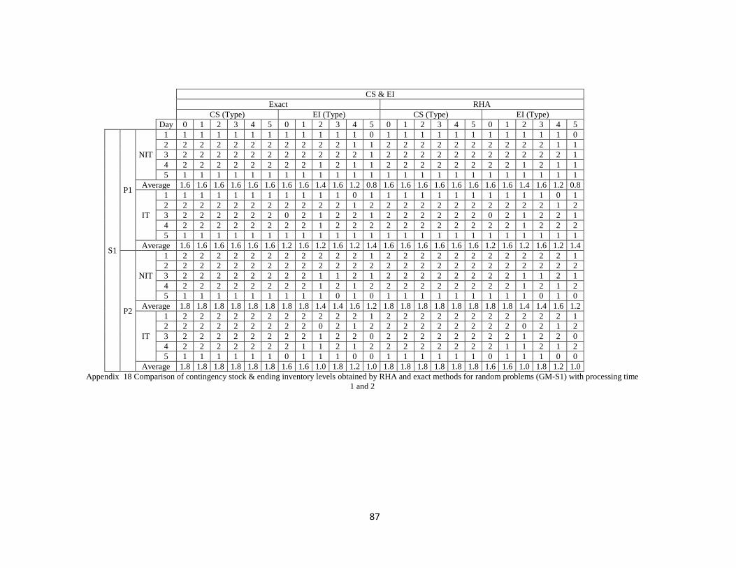
87
CS & EI
Exact RHA
CS (Type) EI (Type) CS (Type) EI (Type)
Day 0 1 2 3 4 5 0 1 2 3 4 5 0 1 2 3 4 5 0 1 2 3 4 5
S1
P1
NIT
1 1 1 1 1 1 1 1 1 1 1 1 0 1 1 1 1 1 1 1 1 1 1 1 0
2 2 2 2 2 2 2 2 2 2 2 1 1 2 2 2 2 2 2 2 2 2 2 1 1
3 2 2 2 2 2 2 2 2 2 2 2 1 2 2 2 2 2 2 2 2 2 2 2 1
4 2 2 2 2 2 2 2 2 1 2 1 1 2 2 2 2 2 2 2 2 1 2 1 1
5 1 1 1 1 1 1 1 1 1 1 1 1 1 1 1 1 1 1 1 1 1 1 1 1
Average 1.6 1.6 1.6 1.6 1.6 1.6 1.6 1.6 1.4 1.6 1.2 0.8 1.6 1.6 1.6 1.6 1.6 1.6 1.6 1.6 1.4 1.6 1.2 0.8
IT
1 1 1 1 1 1 1 1 1 1 1 0 1 1 1 1 1 1 1 1 1 1 1 0 1
2 2 2 2 2 2 2 2 2 2 2 1 2 2 2 2 2 2 2 2 2 2 2 1 2
3 2 2 2 2 2 2 0 2 1 2 2 1 2 2 2 2 2 2 0 2 1 2 2 1
4 2 2 2 2 2 2 2 2 1 2 2 2 2 2 2 2 2 2 2 2 1 2 2 2
5 1 1 1 1 1 1 1 1 1 1 1 1 1 1 1 1 1 1 1 1 1 1 1 1
Average 1.6 1.6 1.6 1.6 1.6 1.6 1.2 1.6 1.2 1.6 1.2 1.4 1.6 1.6 1.6 1.6 1.6 1.6 1.2 1.6 1.2 1.6 1.2 1.4
P2
NIT
1 2 2 2 2 2 2 2 2 2 2 2 1 2 2 2 2 2 2 2 2 2 2 2 1
2 2 2 2 2 2 2 2 2 2 2 2 2 2 2 2 2 2 2 2 2 2 2 2 2
3 2 2 2 2 2 2 2 2 1 1 2 1 2 2 2 2 2 2 2 2 1 1 2 1
4 2 2 2 2 2 2 2 2 1 2 1 2 2 2 2 2 2 2 2 2 1 2 1 2
5 1 1 1 1 1 1 1 1 1 0 1 0 1 1 1 1 1 1 1 1 1 0 1 0
Average 1.8 1.8 1.8 1.8 1.8 1.8 1.8 1.8 1.4 1.4 1.6 1.2 1.8 1.8 1.8 1.8 1.8 1.8 1.8 1.8 1.4 1.4 1.6 1.2
IT
1 2 2 2 2 2 2 2 2 2 2 2 1 2 2 2 2 2 2 2 2 2 2 2 1
2 2 2 2 2 2 2 2 2 0 2 1 2 2 2 2 2 2 2 2 2 0 2 1 2
3 2 2 2 2 2 2 2 2 1 2 2 0 2 2 2 2 2 2 2 2 1 2 2 0
4 2 2 2 2 2 2 2 1 1 2 1 2 2 2 2 2 2 2 2 1 1 2 1 2
5 1 1 1 1 1 1 0 1 1 1 0 0 1 1 1 1 1 1 0 1 1 1 0 0
Average 1.8 1.8 1.8 1.8 1.8 1.8 1.6 1.6 1.0 1.8 1.2 1.0 1.8 1.8 1.8 1.8 1.8 1.8 1.6 1.6 1.0 1.8 1.2 1.0
Appendix 18 Comparison of contingency stock & ending inventory levels obtained by RHA and exact methods for random problems (GM-S1) with processing time
1 and 2

88
Average Mean and Max. Inventory Levels
Exact RHA
Type 0 Type 1 Type 2 Type 3 Type 4 Type 5 Total
Type 0 Type 1 Type 2 Type 3 Type 4 Type 5 Total
Day Mn. Mx. Mn. Mx. Mn. Mx. Mn. Mx. Mn. Mx. Mn. Mx. Mn. Mx. Mn. Mx. Mn. Mx. Mn. Mx. Mn. Mx. Mn. Mx.
S1
P1
NIT
1 1.40 4 3.35 6 2.69 4 1.38 2 1.03 2 0.22 1 10.07 2.00 4 2.56 4 1.94 4 1.25 3 1.26 2 0.15 1 9.17
2 3.81 9 2.06 5 3.06 5 2.45 4 1.27 2 1.50 2 14.15 3.48 6 2.59 5 2.89 4 2.58 4 1.27 2 1.35 2 14.15
3 4.52 9 3.43 6 2.02 3 1.52 3 2.51 3 1.93 3 15.93 2.12 5 3.26 7 2.61 3 2.72 4 2.19 3 1.29 2 14.19
4 2.04 4 4.55 8 1.20 2 1.51 3 1.73 2 1.63 3 12.68 3.07 5 3.53 5 1.84 4 2.74 4 1.46 2 1.46 2 14.10
5 1.97 4 2.08 4 1.66 3 1.12 2 1.37 3 0.73 1 8.93 1.90 4 3.12 6 1.46 3 1.22 3 0.90 2 0.73 1 9.33
Average 2.75 3.10 2.13 1.60 1.58 1.20 2.51 3.01 2.15 2.10 1.42 1.00
IT
1 1.65 5 2.77 6 2.90 5 0.33 1 0.23 1 0.38 1 8.25 0.80 3 1.36 4 0.68 2 1.03 2 0.23 1 0.38 1 4.47
2 0.38 3 1.39 5 0.53 2 2.73 4 1.27 2 1.03 2 7.33 3.35 8 1.67 3 0.71 2 1.23 3 1.27 2 1.03 2 9.25
3 0.45 2 2.18 5 1.07 2 0.83 2 1.56 2 1.10 2 7.20 1.63 4 1.27 3 1.41 2 0.73 2 1.56 2 1.10 2 7.68
4 1.60 3 3.04 6 0.90 2 1.02 2 0.82 2 0.95 2 8.32 1.50 4 2.82 6 1.06 2 1.02 2 0.82 2 1.34 2 8.55
5 1.08 3 0.77 4 0.32 1 1.10 2 0.42 2 0.00 1 3.68 0.99 3 0.63 2 0.55 2 0.33 1 0.70 2 0.06 1 3.25
Average 1.03 2.03 1.15 1.20 0.86 0.69 1.66 1.55 0.88 0.86 0.91 0.78
P2
NIT
1 2.39 4 3.31 7 2.85 5 1.60 3 1.34 2 0.90 2 12.39 3.08 6 2.62 4 1.75 4 1.91 3 2.03 3 1.05 2 12.43
2 3.77 7 2.66 4 1.49 3 1.68 3 1.56 2 1.76 3 12.92 3.62 7 2.78 6 1.34 3 2.20 3 1.56 2 1.38 3 12.88
3 1.48 4 2.62 5 1.41 2 2.22 4 2.20 3 1.75 2 11.68 1.86 4 3.58 7 1.61 2 1.68 3 1.70 2 1.11 2 11.53
4 3.38 6 3.60 6 1.05 2 2.24 4 1.18 2 1.32 2 12.77 2.13 4 3.09 5 1.20 2 2.39 4 1.25 2 2.20 3 12.27
5 2.05 4 1.56 3 0.83 2 0.18 1 0.74 2 0.00 1 5.37 1.45 3 2.11 5 0.37 1 0.72 2 0.75 2 0.00 1 5.40
Average 2.62 2.75 1.53 1.58 1.40 1.15 2.43 2.84 1.25 1.78 1.46 1.15
IT
1 2.05 4 1.61 4 0.42 2 2.10 3 1.11 2 1.42 2 8.70 1.45 2 2.47 4 0.62 2 1.86 3 1.95 3 0.85 2 9.21
2 0.69 3 1.96 5 0.50 2 1.08 2 1.27 2 1.05 2 6.54 1.26 3 2.49 5 0.53 2 1.19 3 1.27 2 1.05 2 7.79
3 0.82 3 0.32 2 1.07 2 2.41 4 1.56 2 1.04 2 7.22 2.51 4 1.16 4 1.07 2 0.88 2 1.68 2 1.04 2 8.35
4 2.01 4 0.85 4 0.95 2 1.03 2 0.91 2 0.79 2 6.54 1.64 3 1.92 4 0.95 2 1.03 2 0.98 2 0.79 2 7.31
5 0.47 2 1.34 3 0.60 2 0.38 2 0.38 1 0.00 1 3.18 0.97 2 0.61 2 0.65 2 0.38 2 0.43 1 0.00 1 3.05
Average 1.21 1.21 0.71 1.40 1.05 0.86 1.57 1.73 0.76 1.07 1.26 0.75
Appendix 19 Comparison of average mean and max. inventory levels obtained by RHA and exact methods for random problems (GM-S1) with processing time 1 and 2

89
CS & EI
TPA RHA
CS (Type) EI (Type) CS (Type) EI (Type)
Day 0 1 2 3 0 1 2 3 0 1 2 3 0 1 2 3
P1
NIT
1
1 1 1 1 0 0 0 0 1 1 1 1 1 1 1 1
1 1 1 1 0 0 0 0 1 1 1 1 1 1 1 1
1 1 1 1 0 0 0 0 1 1 1 1 1 1 1 1
2
1 1 1 1 0 0 0 0 1 1 1 1 1 1 1 1
1 1 1 1 0 0 0 0 1 1 1 1 1 1 1 0
1 1 1 1 0 0 0 0 1 1 1 1 1 1 1 1
3
1 1 1 1 0 0 0 0 1 1 1 1 1 1 1 0
1 1 1 1 0 0 0 0 1 1 1 1 1 1 1 1
1 1 1 1 0 0 0 0 1 1 1 1 1 1 1 1
Avg. 1.00 1.00 1.00 1.00 0.00 0.00 0.00 0.00 1.00 1.00 1.00 1.00 1.00 1.00 1.00 0.78
IT
1
1 1 1 1 1 1 1 1 1 1 1 1 1 1 1 1
1 1 1 1 1 1 1 1 1 1 1 1 1 1 1 1
1 1 1 1 0 0 0 1 1 1 1 1 1 1 1 1
2
1 1 1 1 1 1 1 1 1 1 1 1 1 1 1 1
1 1 1 1 0 0 0 0 1 1 1 1 1 1 1 1
1 1 1 1 1 1 1 1 1 1 1 1 1 1 1 0
3
1 1 1 1 1 1 1 1 1 1 1 1 1 1 1 1
1 1 1 1 1 1 1 1 1 1 1 1 1 1 1 1
1 1 1 1 1 1 1 1 1 1 1 1 1 1 1 1
Avg. 1.00 1.00 1.00 1.00 0.78 0.78 0.78 0.89 1.00 1.00 1.00 1.00 1.00 1.00 1.00 0.89
Appendix 20 Comparison of contingency stock & ending inventory levels obtained by TPA and RHA for real problems with processing time 1

90
CS & EI
TPA RHA
CS (Type) EI (Type) CS (Type) EI (Type)
Day 0 1 2 3 0 1 2 3 0 1 2 3 0 1 2 3
P2
NIT
1
1 1 1 2 0 0 0 0 1 1 1 1 0 1 1 1
1 2 1 1 0 0 0 0 1 1 1 1 1 1 1 0
1 1 1 1 0 0 0 0 1 1 1 1 0 1 0 0
2
1 2 2 1 0 0 0 0 1 1 1 1 0 1 0 0
1 2 2 1 0 0 0 0 2 2 2 2 1 2 2 1
1 2 1 1 0 0 0 0 2 2 2 2 2 2 2 1
3
1 2 1 2 0 0 0 0 1 1 1 1 0 0 0 1
1 1 1 1 0 0 0 0 1 1 1 1 1 1 1 1
1 1 1 1 1 1 1 1 1 1 1 1 1 0 1 0
Avg. 1.00 1.56 1.22 1.22 0.11 0.11 0.11 0.11 1.22 1.22 1.22 1.22 0.67 1.00 0.89 0.56
IT
1
1 1 1 2 1 1 1 1 1 1 1 1 0 1 0 1
1 2 1 1 1 1 1 1 1 1 1 1 1 1 0 0
1 2 2 1 1 1 1 0 2 2 2 2 1 2 0 0
2
1 2 2 1 1 1 1 1 2 2 2 2 0 2 2 1
1 2 2 1 1 1 1 0 2 2 2 2 2 2 0 0
3 5 3 2 1 1 1 1 2 2 2 2 2 1 2 0
3
2 3 2 2 1 1 1 1 2 2 2 2 2 2 1 0
1 1 1 1 1 1 1 0 1 1 1 1 1 0 1 1
1 1 1 1 1 1 1 1 1 1 1 1 1 0 0 1
Avg. 1.33 2.11 1.67 1.33 1.00 1.00 1.00 0.67 1.56 1.56 1.56 1.56 1.11 1.22 0.67 0.44
Appendix 21 Comparison of contingency stock & ending inventory levels obtained by TPA and RHA for real problems with processing time 2

91
CPU Time sec.
# of Setup
TPA RHA
Day TPA RHA M/C. 1 M/C. 2 Total M/C. 1 M/C. 2 Total
P1
NIT
1
7 3 3 5 8 12 1 13
12 6 11 1 12 13 1 14
12 12 4 5 9 11 1 12
2
12 4 3 5 8 10 2 12
19 6 6 2 8 9 2 11
21 5 7 1 8 10 2 12
3
16 6 3 5 8 9 2 11
9 2 10 1 11 12 1 13
9 6 9 2 11 10 2 12
Avg. 13 6 6.2 3.0 9.2 10.7 1.6 12.2
IT
1
18 14 7 3 10 7 1 8
22 23 6 3 9 8 1 9
25 33 6 4 10 8 2 10
2
37 24 8 3 11 5 3 8
34 14 10 2 12 8 1 9
41 21 8 3 11 9 1 10
3
40 23 8 4 12 7 3 10
37 23 9 2 11 7 2 9
22 22 6 4 10 5 4 9
Avg. 31 22 7.6 3.1 10.7 7.1 2.0 9.1
Appendix 22 Comparison of for CPU time and number of setups obtained by TPA and RHA for real problems with processing time 1

92
CPU Time sec.
# of Setup
TPA RHA
Day TPA RHA M/C. 1 M/C. 2 Total M/C. 1 M/C. 2 Total
P2
NIT
1
6 3 7 2 10 9 4 13
14 5 6 4 8 7 5 12
9 4 9 2 10 9 3 12
2
7 3 7 2 12 10 4 14
19 6 5 4 6 7 1 8
17 10 6 4 6 8 3 11
3
39 3 8 2 15 10 5 15
9 3 8 2 8 9 4 13
18 5 9 4 8 8 3 11
Avg. 15 5 7.2 2.9 9.2 8.6 3.6 12.1
IT
1
14 3 7 4 8 10 5 15
15 6 7 5 7 11 4 15
18 17 8 4 5 7 1 8
2
18 5 8 6 5 8 3 11
15 15 9 4 6 6 1 7
102 17 6 3 6 7 2 9
3
15 13 8 4 6 6 3 9
8 11 5 4 8 6 5 11
15 8 8 6 8 7 5 12
Avg. 25 11 7.3 4.4 6.6 7.6 3.2 10.8
Appendix 23 Comparison of CPU time and number of setups obtained by TPA and RHA for real problems with processing time 2

93
Average Mean and Max. Inventory Levels
TPA RHA
Type 0 Type 1 Type 2 Type 3 Total
Type 0 Type 1 Type 2 Type 3 Total
Day Mn. Mx. Mn. Mx. Mn. Mx. Mn. Mx. Mn. Mx. Mn. Mx. Mn. Mx. Mn. Mx.
P1
NIT
1
1.12 3 2.26 5 2.43 5 0.69 2 6.49 1.62 3 4.26 8 1.73 3 0.89 2 8.49
0.59 2 4.58 9 0.88 3 0.26 1 6.31 1.52 3 4.34 8 1.71 3 1.21 2 8.77
1.52 4 1.88 4 2.86 6 0.71 2 6.97 1.67 3 3.99 7 2.21 4 0.84 2 8.71
2
1.21 3 1.98 4 2.48 5 0.68 2 6.35 2.54 5 2.50 5 1.80 3 0.80 2 7.64
1.51 3 3.27 7 2.12 4 0.45 1 7.35 2.30 5 3.40 6 1.96 4 0.32 1 7.98
1.75 4 3.74 7 1.56 4 0.52 1 7.57 2.24 4 4.27 8 1.83 4 0.80 2 9.14
3
1.03 3 1.87 4 2.43 5 0.60 2 5.92 2.59 5 2.68 5 1.60 3 0.21 1 7.08
3.12 6 1.02 3 1.19 4 0.30 1 5.64 1.92 3 4.12 8 1.71 4 0.90 2 8.65
2.81 6 1.70 5 0.92 3 0.37 1 5.81 2.31 4 3.95 7 1.95 4 0.89 2 9.11
Avg. 1.63 2.48 1.87 0.51 6.49 2.08 3.72 1.83 0.76 8.40
IT
1
0.68 2 0.56 2 0.55 2 0.68 2 2.46 0.51 2 0.08 1 0.66 2 0.35 1 1.60
0.52 2 0.61 2 0.78 2 0.70 2 2.62 0.66 3 0.07 1 0.64 2 0.39 1 1.76
0.41 2 0.77 2 0.49 2 0.80 2 2.46 0.96 3 0.54 2 0.77 2 0.27 1 2.54
2
0.61 2 0.66 2 0.74 2 0.80 2 2.81 0.97 3 0.40 2 0.74 2 0.39 1 2.50
0.34 2 0.22 2 0.34 2 0.16 1 1.05 0.96 3 0.18 2 0.78 3 0.28 1 2.20
0.66 3 0.48 3 0.38 2 0.38 1 1.90 0.61 3 0.22 2 0.66 2 0.13 1 1.62
3
0.41 2 0.59 2 0.37 1 0.72 2 2.09 0.43 2 0.22 2 0.98 3 0.22 1 1.85
0.72 2 0.45 2 0.47 2 0.40 2 2.03 0.06 1 0.68 2 0.71 3 0.55 2 2.00
0.49 2 0.70 2 0.36 2 0.73 2 2.28 0.63 3 1.08 3 0.62 2 0.59 2 2.91
Avg. 0.54 0.56 0.50 0.60 2.19 0.64 0.39 0.73 0.35 2.11
Appendix 24 Comparison of average mean and max. inventory levels obtained by TPA and RHA methods for real problems with processing time 1

94
Average Mean and Max. Inventory Levels
TPA RHA
Type 0 Type 1 Type 2 Type 3 Total
Type 0 Type 1 Type 2 Type 3 Total
Day Mn. Mx. Mn. Mx. Mn. Mx. Mn. Mx. Mn. Mx. Mn. Mx. Mn. Mx. Mn. Mx.
P2
NIT
1
1.33 3 0.70 2 1.02 3 0.59 2 3.65 0.40 1 2.04 5 1.13 3 0.75 2 4.31
1.09 2 1.91 4 1.21 3 0.46 1 4.67 1.26 3 1.73 3 1.43 3 0.25 1 4.66
0.98 3 1.28 3 1.07 3 0.16 1 3.49 0.56 2 2.05 4 0.96 3 0.23 1 3.80
2
0.98 2 2.22 5 0.87 2 0.46 1 4.54 0.79 2 1.60 4 0.53 2 0.06 1 2.97
1.11 3 1.06 3 1.88 4 0.56 1 4.60 1.04 2 3.61 6 2.06 4 0.81 2 7.52
0.83 2 1.50 4 1.28 3 0.54 1 4.15 1.90 4 3.09 5 1.97 4 0.95 2 7.91
3
1.18 3 1.23 3 0.68 2 0.57 2 3.65 0.61 2 0.94 3 0.44 2 0.35 1 2.34
1.00 3 2.23 5 0.82 3 0.18 1 4.23 1.90 4 1.89 4 1.07 3 0.68 2 5.55
1.15 3 1.92 5 0.82 2 0.82 2 4.71 1.97 5 0.77 2 0.98 2 0.45 1 4.17
Avg. 1.07 1.56 1.07 0.48 4.19 1.16 1.97 1.17 0.50 4.80
IT
1
0.71 2 0.61 2 0.53 2 0.92 2 2.77 0.24 1 0.09 1 0.35 2 0.37 1 1.05
0.56 2 0.85 2 0.38 1 0.72 2 2.52 0.39 2 0.56 2 0.25 1 0.27 1 1.46
0.92 2 0.64 3 0.76 2 0.60 1 2.92 0.90 3 0.90 3 0.82 2 0.85 2 3.47
2
0.55 2 0.56 2 0.83 2 0.87 2 2.81 0.58 2 0.85 2 1.17 3 1.23 2 3.84
0.58 2 0.46 2 0.82 2 0.58 1 2.44 1.00 3 0.90 2 0.99 3 0.41 2 3.30
1.72 3 1.41 5 1.01 3 1.01 2 5.14 1.06 2 1.21 2 1.45 3 0.51 2 4.24
3
1.10 3 1.07 3 0.63 2 1.18 2 3.97 1.24 4 0.92 2 0.84 2 0.93 2 3.94
0.70 2 0.82 2 0.52 2 0.62 2 2.65 0.62 2 0.53 2 0.45 2 0.31 1 1.92
0.75 2 0.54 2 0.39 2 0.75 2 2.42 0.46 2 0.29 2 0.32 2 0.28 1 1.35
Avg. 0.84 0.77 0.65 0.81 3.07 0.72 0.69 0.74 0.57 2.73
Appendix 25 Comparison of average mean and max. inventory levels obtained by TPA and RHA methods for real problems with processing time 2

95
CS & EI
TPA RHA
CS (Type) EI (Type) CS (Type) EI (Type)
Day 0 1 2 3 4 5 0 1 2 3 4 5 0 1 2 3 4 5 0 1 2 3 4 5
S1
P1
NIT
1 1 1 1 1 1 1 0 0 0 0 0 0 1 1 1 1 1 1 1 1 1 1 1 0
2 2 2 2 2 2 2 0 0 0 0 1 1 2 2 2 2 2 2 2 2 2 2 1 1
3 2 2 2 2 2 2 0 0 1 1 2 1 2 2 2 2 2 2 2 2 2 2 2 1
4 2 2 2 2 2 2 0 0 1 1 1 1 2 2 2 2 2 2 2 2 1 2 1 1
5 1 1 1 1 1 1 0 0 0 0 0 0 1 1 1 1 1 1 1 1 1 1 1 1
Avr.
1.60 1.60 1.60 1.60 1.60 1.60 0.00 0.00 0.40 0.40 0.80 0.60 1.60 1.60 1.60 1.60 1.60 1.60 1.60 1.60 1.40 1.60 1.20 0.80
IT
1 1 1 1 1 1 1 1 1 1 1 0 1 1 1 1 1 1 1 1 1 1 1 0 1
2 2 2 2 2 2 2 1 1 1 1 1 1 2 2 2 2 2 2 2 2 2 2 1 2
3 2 2 2 2 2 2 1 1 1 1 1 0 2 2 2 2 2 2 0 2 1 2 2 1
4 2 2 2 2 2 2 1 1 1 1 1 1 2 2 2 2 2 2 2 2 1 2 2 2
5 1 1 1 1 1 1 1 1 1 0 0 1 1 1 1 1 1 1 1 1 1 1 1 1
Avr.
1.60 1.60 1.60 1.60 1.60 1.60 1.00 1.00 1.00 0.80 0.60 0.80 1.60 1.60 1.60 1.60 1.60 1.60 1.20 1.60 1.20 1.60 1.20 1.40
P2
NIT
1 2 2 2 2 2 2 1 1 1 0 0 1 2 2 2 2 2 2 2 2 2 2 2 1
2 2 2 2 2 2 2 0 0 0 0 1 1 2 2 2 2 2 2 2 2 2 2 2 2
3 2 2 2 2 2 2 0 0 1 1 2 1 2 2 2 2 2 2 2 2 1 1 2 1
4 2 2 2 2 2 2 0 0 1 1 1 1 2 2 2 2 2 2 2 2 1 2 1 2
5 1 1 1 1 1 1 0 0 0 0 0 0 1 1 1 1 1 1 1 1 1 0 1 0
Avr.
1.80 1.80 1.80 1.80 1.80 1.80 0.20 0.20 0.60 0.40 0.80 0.80 1.80 1.80 1.80 1.80 1.80 1.80 1.80 1.80 1.40 1.40 1.60 1.20
IT
1 2 2 2 2 2 2 1 1 1 1 1 1 2 2 2 2 2 2 2 2 2 2 2 1
2 2 2 2 2 2 2 1 1 0 1 1 1 2 2 2 2 2 2 2 2 0 2 1 2
3 2 2 2 2 2 2 1 1 0 0 1 0 2 2 2 2 2 2 2 2 1 2 2 0
4 2 2 2 2 2 2 1 1 1 1 0 1 2 2 2 2 2 2 2 1 1 2 1 2
5 1 1 2 1 1 1 1 1 0 0 0 1 1 1 1 1 1 1 0 1 1 1 0 0
Avr.
1.80 1.80 2.00 1.80 1.80 1.80 1.00 1.00 0.40 0.60 0.60 0.80 1.80 1.80 1.80 1.80 1.80 1.80 1.60 1.60 1.00 1.80 1.20 1.00
Appendix 26 Comparison of contingency stock & ending inventory levels obtained by TPA and RHA for random problems (GM-S1) with processing time 1 and 2

96
CS & EI
TPA RHA
CS (Type) EI (Type) CS (Type) EI (Type)
Day 0 1 2 3 4 5 0 1 2 3 4 5 0 1 2 3 4 5 0 1 2 3 4 5
S1
P1
NIT
1 1 1 1 1 1 1 0 0 0 0 0 0 1 1 1 1 1 1 1 1 1 1 1 0
2 2 2 2 2 2 2 0 0 0 0 1 1 2 2 2 2 2 2 2 2 2 2 1 1
3 2 2 2 2 2 2 0 0 1 1 2 1 2 2 2 2 2 2 2 2 2 2 2 1
4 2 2 2 2 2 2 0 0 1 1 1 1 2 2 2 2 2 2 2 2 1 2 1 1
5 1 1 1 1 1 1 0 0 0 0 0 0 1 1 1 1 1 1 1 1 1 1 1 1
Avr.
1.60 1.60 1.60 1.60 1.60 1.60 0.00 0.00 0.40 0.40 0.80 0.60 1.60 1.60 1.60 1.60 1.60 1.60 1.60 1.60 1.40 1.60 1.20 0.80
IT
1 1 1 1 1 1 1 1 1 1 1 0 1 1 1 1 1 1 1 1 1 1 1 0 1
2 2 2 2 2 2 2 1 1 1 1 1 1 2 2 2 2 2 2 2 2 2 2 1 2
3 2 2 2 2 2 2 1 1 1 1 1 0 2 2 2 2 2 2 0 2 1 2 2 1
4 2 2 2 2 2 2 1 1 1 1 1 1 2 2 2 2 2 2 2 2 1 2 2 2
5 1 1 1 1 1 1 1 1 1 0 0 1 1 1 1 1 1 1 1 1 1 1 1 1
Avr.
1.60 1.60 1.60 1.60 1.60 1.60 1.00 1.00 1.00 0.80 0.60 0.80 1.60 1.60 1.60 1.60 1.60 1.60 1.20 1.60 1.20 1.60 1.20 1.40
P2
NIT
1 2 2 2 2 2 2 1 1 1 0 0 1 2 2 2 2 2 2 2 2 2 2 2 1
2 2 2 2 2 2 2 0 0 0 0 1 1 2 2 2 2 2 2 2 2 2 2 2 2
3 2 2 2 2 2 2 0 0 1 1 2 1 2 2 2 2 2 2 2 2 1 1 2 1
4 2 2 2 2 2 2 0 0 1 1 1 1 2 2 2 2 2 2 2 2 1 2 1 2
5 1 1 1 1 1 1 0 0 0 0 0 0 1 1 1 1 1 1 1 1 1 0 1 0
Avr.
1.80 1.80 1.80 1.80 1.80 1.80 0.20 0.20 0.60 0.40 0.80 0.80 1.80 1.80 1.80 1.80 1.80 1.80 1.80 1.80 1.40 1.40 1.60 1.20
IT
1 2 2 2 2 2 2 1 1 1 1 1 1 2 2 2 2 2 2 2 2 2 2 2 1
2 2 2 2 2 2 2 1 1 0 1 1 1 2 2 2 2 2 2 2 2 0 2 1 2
3 2 2 2 2 2 2 1 1 0 0 1 0 2 2 2 2 2 2 2 2 1 2 2 0
4 2 2 2 2 2 2 1 1 1 1 0 1 2 2 2 2 2 2 2 1 1 2 1 2
5 1 1 2 1 1 1 1 1 0 0 0 1 1 1 1 1 1 1 0 1 1 1 0 0
Avr.
1.80 1.80 2.00 1.80 1.80 1.80 1.00 1.00 0.40 0.60 0.60 0.80 1.80 1.80 1.80 1.80 1.80 1.80 1.60 1.60 1.00 1.80 1.20 1.00
Appendix 27 Comparison of contingency stock & ending inventory levels obtained by TPA and RHA for random problems (GM-S1) with processing time 1 and 2
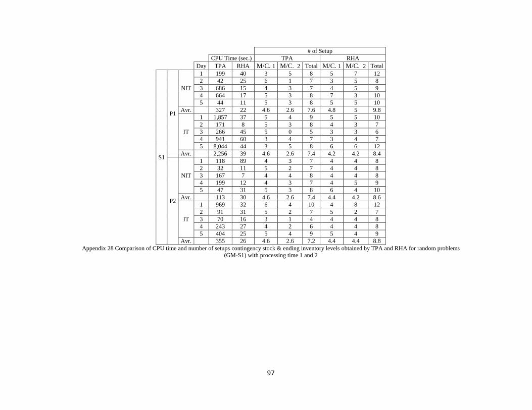
97
# of Setup
CPU Time (sec.) TPA RHA
Day TPA RHA M/C. 1 M/C. 2 Total M/C. 1 M/C. 2 Total
S1
P1
NIT
1 199 40 3 5 8 5 7 12
2 42 25 6 1 7 3 5 8
3 686 15 4 3 7 4 5 9
4 664 17 5 3 8 7 3 10
5 44 11 5 3 8 5 5 10
Avr.
327 22 4.6 2.6 7.6 4.8 5 9.8
IT
1 1,857 37 5 4 9 5 5 10
2 171 8 5 3 8 4 3 7
3 266 45 5 0 5 3 3 6
4 941 60 3 4 7 3 4 7
5 8,044 44 3 5 8 6 6 12
Avr.
2,256 39 4.6 2.6 7.4 4.2 4.2 8.4
P2
NIT
1 118 89 4 3 7 4 4 8
2 32 11 5 2 7 4 4 8
3 167 7 4 4 8 4 4 8
4 199 12 4 3 7 4 5 9
5 47 31 5 3 8 6 4 10
Avr.
113 30 4.6 2.6 7.4 4.4 4.2 8.6
IT
1 969 32 6 4 10 4 8 12
2 91 31 5 2 7 5 2 7
3 70 16 3 1 4 4 4 8
4 243 27 4 2 6 4 4 8
5 404 25 5 4 9 5 4 9
Avr.
355 26 4.6 2.6 7.2 4.4 4.4 8.8
Appendix 28 Comparison of CPU time and number of setups contingency stock & ending inventory levels obtained by TPA and RHA for random problems
(GM-S1) with processing time 1 and 2

98
Average Mean and Max. Inventory Levels
TPA RHA
Type 0 Type 1 Type 2 Type 3 Type 4 Type 5 Type 0 Type 1 Type 2 Type 3 Type 4 Type 5 Total
Day Mn. Mx. Mn. Mx. Mn. Mx. Mn. Mx. Mn. Mx. Mn. Mx. Total Mn. Mx. Mn. Mx. Mn. Mx. Mn. Mx. Mn. Mx. Mn. Mx.
S1
P1
NIT
1 1.1 4 1.4 4 1.9 4 1.2 3 0.4 1 0.2 1 6.3 2.0 4 2.6 4 1.9 4 1.3 3 1.3 2 0.2 1 9.2
2 1.6 4 2.4 5 0.6 2 0.6 3 1.3 2 1.9 2 8.4 3.5 6 2.6 5 2.9 4 2.6 4 1.3 2 1.3 2 14.2
3 2.3 6 2.8 7 1.4 2 1.3 2 2.5 3 1.9 3 12.2 2.1 5 3.3 7 2.6 3 2.7 4 2.2 3 1.3 2 14.2
4 2.3 5 2.2 4 1.6 4 1.6 2 1.7 2 1.6 3 11.2 3.1 5 3.5 5 1.8 4 2.7 4 1.5 2 1.5 2 14.1
5 2.4 4 2.0 5 0.3 2 0.3 1 1.1 2 0.0 1 6.0 1.9 4 3.1 6 1.5 3 1.2 3 0.9 2 0.7 1 9.3
Avr. 1.9 2.2 1.2 1.0 1.4 1.1 2.5 3.0 2.1 2.1 1.4 1.0
IT
1 0.7 2 0.2 1 0.5 1 1.0 2 0.6 1 0.6 1 3.5 0.8 3 1.4 4 0.7 2 1.0 2 0.2 1 0.4 1 4.5
2 2.5 5 0.7 2 1.0 2 0.5 2 1.3 2 1.0 2 7.0 3.4 8 1.7 3 0.7 2 1.2 3 1.3 2 1.0 2 9.3
3 2.1 5 1.3 4 1.1 2 1.0 2 1.6 2 1.0 2 8.0 1.6 4 1.3 3 1.4 2 0.7 2 1.6 2 1.1 2 7.7
4 0.8 2 0.8 3 0.9 2 1.0 2 0.9 2 0.7 2 5.2 1.5 4 2.8 6 1.1 2 1.0 2 0.8 2 1.3 2 8.5
5 2.1 4 0.3 2 0.0 1 0.7 2 0.7 2 0.0 1 3.8 1.0 3 0.6 2 0.5 2 0.3 1 0.7 2 0.1 1 3.3
Avr. 1.6 0.7 0.7 0.8 1.0 0.7 1.7 1.5 0.9 0.9 0.9 0.8
P2
NIT
1 2.8 6 2.4 5 1.6 4 1.1 2 1.1 2 1.3 2 10.3 3.1 6 2.6 4 1.8 4 1.9 3 2.0 3 1.0 2 12.4
2 3.2 7 0.9 3 0.8 2 0.6 2 1.3 2 1.9 2 8.7 3.6 7 2.8 6 1.3 3 2.2 3 1.6 2 1.4 3 12.9
3 1.1 3 1.8 5 2.0 3 2.1 3 2.1 3 1.5 2 10.5 1.9 4 3.6 7 1.6 2 1.7 3 1.7 2 1.1 2 11.5
4 2.2 4 1.4 3 1.8 4 2.2 4 1.3 2 1.3 2 10.3 2.1 4 3.1 5 1.2 2 2.4 4 1.3 2 2.2 3 12.3
5 1.4 3 1.2 3 0.3 2 0.5 1 0.7 2 0.0 1 4.1 1.5 3 2.1 5 0.4 1 0.7 2 0.7 2 0.0 1 5.4
Avr. 2.1 1.6 1.3 1.3 1.3 1.2 2.4 2.8 1.3 1.8 1.5 1.1
IT
1 0.9 2 0.4 2 0.7 2 1.4 2 1.1 2 0.7 2 5.2 1.5 2 2.5 4 0.6 2 1.9 3 2.0 3 0.9 2 9.2
2 0.3 2 0.9 2 0.8 2 0.5 2 1.3 2 1.0 2 4.9 1.3 3 2.5 5 0.5 2 1.2 3 1.3 2 1.0 2 7.8
3 0.4 2 0.2 2 1.1 2 0.7 2 1.6 2 1.0 2 5.0 2.5 4 1.2 4 1.1 2 0.9 2 1.7 2 1.0 2 8.3
4 0.4 2 0.6 2 1.1 2 1.2 2 0.8 2 0.7 2 4.9 1.6 3 1.9 4 1.0 2 1.0 2 1.0 2 0.8 2 7.3
5 0.9 2 0.4 2 0.4 2 0.3 1 0.5 1 0.6 1 3.1 1.0 2 0.6 2 0.6 2 0.4 2 0.4 1 0.0 1 3.0
Avr. 0.6 0.5 0.8 0.8 1.1 0.8 1.6 1.7 0.8 1.1 1.3 0.7
Appendix 29 Comparison of average mean and max. inventory levels obtained by TPA and RHA for random problems (GM-S1) with processing time 1 and 2

99
# of Setup
CPU Time (sec.) TPA RHA
Day TPA RHA M/C. 1 M/C. 2 Total M/C. 1 M/C. 2 Total
S1
P1
NIT
1 31 4 2 6 8 6 3 9
2 39 25 5 4 9 5 5 10
3 70 9 2 5 7 4 7 11
4 43 38 7 3 10 7 5 12
5 16 15 5 3 8 7 5 12
Avr.
40 18 4.2 4.2 8.4 5.8 5.0 10.8
IT
1 49 21 5 4 9 5 3 8
2 1,044 53 5 6 11 5 5 10
3 116 19 4 5 9 6 4 10
4 68 51 5 5 10 5 4 9
5 10 18 5 3 8 6 5 11
Avr.
257 32 4.8 4.6 9.4 5.4 4.2 9.6
P2
NIT
1 46 7 5 2 7 3 6 9
2 39 26 2 5 7 6 4 10
3 25 9 4 2 6 7 2 9
4 33 24 7 3 10 7 5 12
5 8 7 4 2 6 4 6 10
Avr.
30 15 4.4 2.8 7.2 5.4 4.6 10.0
IT
1 31 12 5 3 8 5 3 8
2 175 10 7 5 12 5 4 9
3 117 32 2 5 7 4 6 10
4 247 22 5 4 9 4 6 10
5 11 10 3 4 7 3 4 7
Avr.
116 17 4.4 4.2 8.6 4.2 4.6 8.8
Appendix 30 Comparison of CPU time and number of setups obtained by TPA and RHA for random problems (GM-S2) with processing time 1 and 2

100
CS & EI
TPA RHA
CS (Type) EI (Type) CS (Type) EI (Type)
Day 0 1 2 3 4 5 0 1 2 3 4 5 0 1 2 3 4 5 0 1 2 3 4 5
S1
P1
NIT
1 1 1 1 1 1 1 0 1 0 0 0 0 1 1 1 1 1 1 1 1 1 1 1 1
2 1 1 1 1 1 1 0 0 0 0 0 0 1 1 1 1 1 1 1 1 1 1 1 1
3 1 1 1 1 1 1 0 0 0 0 0 0 1 1 1 1 1 1 1 1 1 1 1 1
4 1 1 1 1 1 1 0 0 0 0 0 0 1 1 1 1 1 1 1 1 1 1 1 1
5 1 1 1 1 1 1 0 0 0 0 0 0 1 1 1 1 1 1 1 1 1 1 1 1
Avr.
1.0 1.0 1.0 1.0 1.0 1.0 0.0 0.2 0.0 0.0 0.0 0.0 1.0 1.0 1.0 1.0 1.0 1.0 1.0 1.0 1.0 1.0 1.0 1.0
IT
1 1 1 1 1 1 1 1 1 1 1 1 1 1 1 1 1 1 1 1 1 1 1 1 1
2 1 1 1 1 1 1 1 1 1 1 1 1 1 1 1 1 1 1 1 0 1 1 1 1
3 1 1 1 1 1 1 1 1 0 1 1 1 1 1 1 1 1 1 1 1 1 1 1 1
4 1 1 1 1 1 1 0 0 0 0 0 0 1 1 1 1 1 1 1 1 1 1 1 1
5 1 1 1 1 1 1 0 0 0 0 0 0 1 1 1 1 1 1 1 1 1 1 1 1
Avr.
1.0 1.0 1.0 1.0 1.0 1.0 0.6 0.6 0.4 0.6 0.6 0.6 1.0 1.0 1.0 1.0 1.0 1.0 1.0 0.8 1.0 1.0 1.0 1.0
P2
NIT
1 2 2 2 2 2 2 0 2 0 1 0 0 2 2 2 2 2 2 2 2 2 2 2 2
2 2 2 2 2 2 2 0 0 1 0 0 0 2 2 2 2 2 2 2 2 2 2 1 2
3 2 2 2 2 2 2 1 1 0 1 0 0 2 2 2 2 2 2 2 2 2 2 2 2
4 1 1 1 1 1 1 0 0 0 0 0 0 1 1 1 1 1 1 1 1 1 1 1 0
5 2 2 2 2 2 2 1 0 0 0 1 0 2 2 2 2 2 2 2 2 2 2 2 2
Avr.
1.8 1.8 1.8 1.8 1.8 1.8 0.4 0.6 0.2 0.4 0.2 0.0 1.8 1.8 1.8 1.8 1.8 1.8 1.8 1.8 1.8 1.8 1.6 1.6
IT
1 2 2 2 2 2 2 1 2 1 1 1 1 2 2 2 2 2 2 2 2 2 2 2 2
2 2 2 2 2 2 2 1 1 1 1 1 1 2 2 2 2 2 2 2 2 2 2 2 2
3 2 2 2 2 2 2 1 1 1 1 1 1 2 2 2 2 2 2 2 2 2 2 2 2
4 1 1 1 1 1 1 1 1 1 1 1 1 1 1 1 1 1 1 1 1 1 1 1 0
5 2 2 2 2 2 2 1 1 1 1 1 1 2 2 2 2 2 2 2 2 2 2 2 2
Avr.
1.8 1.8 1.8 1.8 1.8 1.8 1.0 1.2 1.0 1.0 1.0 1.0 1.8 1.8 1.8 1.8 1.8 1.8 1.8 1.8 1.8 1.8 1.8 1.6
Appendix 31 Comparison of contingency stock & ending inventory levels obtained by TPA and RHA for random problems (GM-S2) with processing time 1 and 2

101
Average Mean and Max. Inventory Levels
TPA RHA
Type 0 Type 1 Type 2 Type 3 Type 4 Type 5
Type 0 Type 1 Type 2 Type 3 Type 4 Type 5 Total
Day Mn. Mx. Mn. Mx. Mn. Mx. Mn. Mx. Mn. Mx. Mn. Mx. Total Mn. Mx. Mn. Mx. Mn. Mx. Mn. Mx. Mn. Mx. Mn. Mx.
S1
P1
NIT
1 1.25 3 2.12 3 2.00 4 0.63 2 1.07 3 0.53 1 7.60 1.70 3 1.68 3 2.09 4 1.25 2 2.63 5 1.40 3 10.75
2 1.15 3 0.58 1 0.96 3 1.96 4 0.76 2 0.98 4 6.38 2.19 4 0.96 2 1.58 4 2.22 4 1.38 2 1.45 4 9.77
3 0.92 3 1.14 2 1.67 5 1.38 3 1.85 5 0.08 1 7.04 1.48 4 1.49 3 2.07 4 2.17 4 1.44 4 0.90 2 9.55
4 0.85 2 1.11 4 0.73 2 1.43 3 0.36 3 1.48 3 5.96 1.23 2 1.40 4 1.71 3 2.69 5 1.09 2 2.05 3 10.16
5 0.22 1 0.57 2 0.89 2 1.39 3 1.47 3 1.43 3 5.97 1.06 2 1.46 3 1.28 2 1.54 3 2.15 4 1.77 3 9.26
Avr.
0.9
1.1
1.2
1.4
1.1
0.9
6.6 1.5
1.4
1.7
2.0
1.7
1.5
9.9
IT
1 0.72 1 0.87 1 0.79 2 0.77 2 0.48 2 0.60 2 4.23 1.08 2 0.87 1 0.79 2 0.62 1 0.38 1 0.58 2 4.30
2 0.70 2 0.89 2 1.05 3 0.73 2 0.90 1 0.23 1 4.50 0.98 2 0.03 1 0.76 1 0.34 1 1.22 3 0.34 1 3.66
3 0.98 2 1.25 3 0.80 2 0.28 1 0.27 2 0.68 1 4.26 0.89 2 0.07 1 0.72 2 0.26 1 0.58 3 0.68 1 3.20
4 0.09 1 0.36 2 0.38 1 0.36 1 0.15 1 0.25 2 1.59 0.36 2 0.94 3 0.46 1 1.50 3 0.80 1 0.25 2 4.30
5 0.22 1 0.10 1 0.33 1 0.30 1 0.50 1 0.61 2 2.05 0.22 1 0.65 1 0.68 2 0.27 2 0.66 2 0.83 2 3.31
Avr.
0.5
0.7
0.7
0.5
0.5
0.5
3.3 0.7
0.5
0.7
0.6
0.7
0.5
3.8
P2
NIT
1 1.33 3 2.77 4 1.73 4 1.51 2 2.16 4 0.85 2 10.35 2.35 3 2.13 3 3.00 5 2.34 3 1.68 4 2.37 3 13.87
2 1.07 3 0.58 2 2.13 4 2.42 5 0.80 2 1.26 4 8.25 2.18 4 2.02 3 1.89 3 2.38 5 1.39 2 1.80 4 11.65
3 1.68 3 2.40 3 1.73 5 1.87 4 2.01 5 0.25 2 9.95 2.44 4 2.03 3 2.40 4 1.68 3 2.48 5 1.96 3 12.98
4 0.50 1 0.68 2 0.55 2 0.66 3 0.28 2 1.31 2 3.98 1.15 2 1.31 3 1.48 3 1.33 3 0.68 2 0.87 2 6.82
5 1.22 2 0.63 2 1.06 2 1.53 3 2.77 4 1.43 3 8.62 1.93 2 2.00 3 2.42 3 2.10 4 2.83 4 2.47 4 13.75
Avr.
1.2
1.4
1.4
1.6
1.6
1.0
8.2 2.0
1.9
2.2
2.0
1.8
1.9
11.8
IT
1 1.28 2 1.88 2 0.68 2 1.00 2 0.27 2 0.50 2 5.60 1.63 3 2.26 4 1.80 4 1.72 3 0.43 3 1.90 3 9.74
2 0.78 2 0.70 2 1.35 2 0.71 2 0.73 2 0.70 2 4.97 2.39 5 0.80 2 1.39 2 1.23 3 0.68 3 2.27 4 8.75
3 1.41 2 0.99 2 1.26 2 0.73 2 0.68 2 0.78 2 5.84 1.52 3 1.78 3 1.58 3 1.37 2 0.97 3 1.85 3 9.07
4 0.67 2 0.56 2 0.51 1 1.09 2 0.82 1 0.80 3 4.44 0.85 2 0.20 1 0.61 2 0.49 1 0.81 1 0.50 2 3.46
5 1.22 2 0.75 2 0.73 2 0.70 2 1.05 2 0.80 2 5.25 2.03 3 1.81 3 1.58 3 0.56 3 1.11 2 1.10 3 8.20
Avr.
1.1
1.0
0.9
0.8
0.7
0.7
5.2 1.7
1.4
1.4
1.1
0.8
1.5
7.8
Appendix 32 Comparison of average mean and max inventory levels obtained by TPA and RHA for random problems (GM-S2) with processing time 1 and 2