Inverse Compton scattering in highenergy astrophysics.

A thesis submitted for the degree ofDoctor of Philosophy

by

Jason Cullen

Research Centre for Theoretical Astrophysics& Theoretical Physics Group

School of PhysicsUniversity of Sydney

Australia

August 2001

Declaration of originality

To the best of my knowledge, this thesis contains no copy or paraphrase of work pub-lished by another person, except where duly acknowledged in the text. This thesiscontains no material which has been presented for a degree at the University of Sydneyor any other university.

Jason Cullen

i

Acknowledgements

I wish to thank Zdenka Kuncic and Kinwah Wu for important suggestions regardingthe work in Chapter 4.

I also wish to thank Chris Rennie for advice on the IDL routine used in Chapter 5.

Thanks also to Roberto Soria for suggesting I work on bulk rotational motion Comp-tonization.

My grateful thanks to my principle supervisor for this thesis, Kinwah Wu.

ii

Abstract

This thesis investigates some aspects of the inverse Compton scattering process withinvarious physical contexts in high energy astrophysics. Initially an introduction to thekey results of Comptonization theory for the case of scattering in optically thick plasmasis given, using a diffusion approach, since these results are required for the interpreta-tion of Comptonized spectra.

Since Comptonization in astrophysical systems is frequently treated using numericaltechniques, an introduction to these is then presented. Such linear Monte Carlo photontransport codes are typically applied to scattering in plasmas without temperature anddensity gradients. Additionally, treating bulk motion can be difficult even for simplecases.

It is demonstrated that these problems can be made tractable numerically with the use ofalgorithms associated with non-linear Monte Carlo codes. Such codes can already treatscattering within arbitrary velocity structures in a plasma, and an extension of the algo-rithm is proposed that enables the easy calculation of photon transport in plasmas withnon-constant density as well as non-constant temperature and/or bulk motion. Thisalgorithm and code has been developed to treat scattering in astrophysical situationswhere bulk motion, temperature gradients and density gradients are simultaneouslypresent in a plasma.

Both a semi-analytic approach and the numerical approach are then used to treat Comp-tonization problems of current interest. Firstly, the standard two-phase disk–coronamodel for the high-energy spectra of Active Galactic Nuclei is modified to include anan outflow or wind which may provide an additional source of disk cooling. Earlierslab disk–corona models predict a spectral index which is consistent with observationsonly if all the accretion power is dissipated in the corona. For the models investigatedhere, energy spectral indices that are consistent with observations can be obtained withless accretion power being dissipated in the corona, as a result of an outflow/wind.However, it is required that the wind extract large amounts of power from the disk, andit it yet to be seen if this is a plausible scenario.

iii

Secondly, the linear numerical technique is then applied to a study of the time delayor lag of high energy photons due to the inverse Compton process, for cases where thescattering plasma is characterised by more than one temperature. Such a model hasbeen proposed for Cyg X-1, and the spectral and temporal behaviour of such a modelis investigated. Predictions are made regarding the form that the time lag curve shouldtake if this particular geometry is a realistic model for the material surrounding Galacticblack hole candidates.

The extended non-linear algorithm is then applied to the study of scattering in bulkmotion accretion flows in both one and two dimensions. The 1-D case is that of linephoton scattering in the accretion column of a magnetised white dwarf star, and theresulting spectra are presented for various inclination angles, accretion rates, and Cy-clotron cooling rates in the post-shock region. Spectra as a function of inclination angleare also obtained and beaming of photons by the inhomogeneous column is investi-gated.

The 2-D case is that of Comptonization in a rotating torus geometry, which is a firstattempt at considering scattering in an orbiting accretion disk-like structure. Differentphoton injection spectra are investigated for different values of the electron momentumwithin the torus. It is found that for a reasonable optical depth and electron momentum,lines can be significantly broadened by rotational Compton scattering.

iv

Contents

I Background 1

1 Theory of Compton scattering 21.1 Introduction . . . . . . . . . . . . . . . . . . . . . . . . . . . . . . . . . . . . 21.2 Compton scattering . . . . . . . . . . . . . . . . . . . . . . . . . . . . . . . . 2

1.2.1 Energy shift . . . . . . . . . . . . . . . . . . . . . . . . . . . . . . . . 21.2.2 Low and high optical depth regimes . . . . . . . . . . . . . . . . . . 41.2.3 Moderate optical depth regime . . . . . . . . . . . . . . . . . . . . . 71.2.4 The stationary equation . . . . . . . . . . . . . . . . . . . . . . . . . 101.2.5 Spectral characteristics . . . . . . . . . . . . . . . . . . . . . . . . . . 11

1.3 Compton scattering in astrophysical objects . . . . . . . . . . . . . . . . . . 121.3.1 Disk-corona systems . . . . . . . . . . . . . . . . . . . . . . . . . . . 131.3.2 Galactic black hole candidates . . . . . . . . . . . . . . . . . . . . . 141.3.3 Accreting magnetic compact stars . . . . . . . . . . . . . . . . . . . 14

1.4 Thesis outline . . . . . . . . . . . . . . . . . . . . . . . . . . . . . . . . . . . 15

II Technical 17

2 Monte Carlo numerical approach 182.1 Monte Carlo photon transport . . . . . . . . . . . . . . . . . . . . . . . . . . 18

2.1.1 Introduction to the Monte Carlo technique . . . . . . . . . . . . . . 202.1.2 von Neumann method . . . . . . . . . . . . . . . . . . . . . . . . . . 212.1.3 Modeling a scattering event . . . . . . . . . . . . . . . . . . . . . . . 222.1.4 The photon transport technique . . . . . . . . . . . . . . . . . . . . 24

2.2 Summary . . . . . . . . . . . . . . . . . . . . . . . . . . . . . . . . . . . . . . 25

3 Photon transport through plasmas with density and velocity structure 273.1 Overview . . . . . . . . . . . . . . . . . . . . . . . . . . . . . . . . . . . . . . 27

v

3.2 Non-linear Monte Carlo simulation . . . . . . . . . . . . . . . . . . . . . . . 283.2.1 Conventional algorithm . . . . . . . . . . . . . . . . . . . . . . . . . 283.2.2 Current non-linear Monte Carlo method . . . . . . . . . . . . . . . 29

3.3 Refined algorithm . . . . . . . . . . . . . . . . . . . . . . . . . . . . . . . . . 313.4 Implementation of the method . . . . . . . . . . . . . . . . . . . . . . . . . 33

3.4.1 An illustrative example . . . . . . . . . . . . . . . . . . . . . . . . . 343.5 Some remarks . . . . . . . . . . . . . . . . . . . . . . . . . . . . . . . . . . . 39

III Astrophysical 42

4 Comptonized Spectra from AGN 434.1 Accretion disk coronae . . . . . . . . . . . . . . . . . . . . . . . . . . . . . . 434.2 A modified two-phase model . . . . . . . . . . . . . . . . . . . . . . . . . . 46

4.2.1 Energy Balance . . . . . . . . . . . . . . . . . . . . . . . . . . . . . . 464.3 Spectral Index and Temperature . . . . . . . . . . . . . . . . . . . . . . . . . 48

4.3.1 Iterative Method . . . . . . . . . . . . . . . . . . . . . . . . . . . . . 484.4 Investigation of a magnetically-heated corona . . . . . . . . . . . . . . . . . 514.5 Dependence of spectral index . . . . . . . . . . . . . . . . . . . . . . . . . . 604.6 Conclusion . . . . . . . . . . . . . . . . . . . . . . . . . . . . . . . . . . . . . 62

5 Time lags due to Comptonization in multi-temperature plasmas surroundingcompact objects 675.1 Compton scattering in galactic black hole candidates . . . . . . . . . . . . 675.2 Description of the numerical approach: galactic black hole candidates . . 695.3 Results: spectra . . . . . . . . . . . . . . . . . . . . . . . . . . . . . . . . . . 725.4 Results: time lags . . . . . . . . . . . . . . . . . . . . . . . . . . . . . . . . . 745.5 Conclusion . . . . . . . . . . . . . . . . . . . . . . . . . . . . . . . . . . . . . 85

6 Compton scattering in bulk accretion flows 896.1 1D: Accretion column . . . . . . . . . . . . . . . . . . . . . . . . . . . . . . . 89

6.1.1 Accretion column in magnetic white dwarf stars . . . . . . . . . . . 896.1.2 Description of the numerical approach: column . . . . . . . . . . . 906.1.3 Results . . . . . . . . . . . . . . . . . . . . . . . . . . . . . . . . . . . 926.1.4 Discussion . . . . . . . . . . . . . . . . . . . . . . . . . . . . . . . . . 94

6.2 2D: Accretion disk . . . . . . . . . . . . . . . . . . . . . . . . . . . . . . . . . 986.2.1 Rotating torus . . . . . . . . . . . . . . . . . . . . . . . . . . . . . . . 98

vi

6.2.2 Description of the numerical approach: disk . . . . . . . . . . . . . 1016.2.3 Results . . . . . . . . . . . . . . . . . . . . . . . . . . . . . . . . . . . 1036.2.4 Discussion . . . . . . . . . . . . . . . . . . . . . . . . . . . . . . . . . 113

6.3 Conclusion . . . . . . . . . . . . . . . . . . . . . . . . . . . . . . . . . . . . . 117

7 Conclusions 119

IV Appendix 122

A Monte Carlo photon transport code 123

vii

List of Figures

2.1 Illustration of the basic direct inversion Monte Carlo method . . . . . . . . 21

3.1 Test runs comparing the output spectrum of the non-linear and the linearcode for a sphere of plasma, of different optical depths. Log of intensityis on the vertical axis and log of photon energy is on the horizontal axis. . 32

3.2 Scattering of a 6.4 keV line by cold electrons. . . . . . . . . . . . . . . . . . 353.3 Scattering of a 6.4 keV line by freely-falling electrons. . . . . . . . . . . . . 363.4 Scattering of power law photons by cold electrons with constant density

and by electrons with a density gradient. . . . . . . . . . . . . . . . . . . . 373.5 Scattering of power law photons by freely-falling electrons. . . . . . . . . . 383.6 Bulk motion scattering for � = 0:001, and thermal scattering for � = 0:001,

for blackbody source photons. . . . . . . . . . . . . . . . . . . . . . . . . . . 40

4.1 A schematic illustration of the energy balance for the modified two-phasemodel used in this work. If PW = 0 the conventional disk–corona modelis recovered (Haardt & Maraschi 1991). . . . . . . . . . . . . . . . . . . . . 47

4.2 (a, top panel) Spectral index as a function of the total optical depth for f= 0.5, a = 0:15, � = 0:6 and various values of �, calculated using the am-plification factor in Section 2.1. (b, bottom panel) Corresponding curvesfor the electron temperature of the corona as a function of the total opticaldepth. . . . . . . . . . . . . . . . . . . . . . . . . . . . . . . . . . . . . . . . . 52

4.3 (a, top panel) Spectral index as a function of the total optical depth for� = 0:75, a = 0:15, � = 0:6 and various values of f . (b, bottom panel) Cor-responding curves for the electron temperature of the corona as a func-tion of the total optical depth . . . . . . . . . . . . . . . . . . . . . . . . . . . 53

viii

4.4 (a, top panel) Spectral index as a function of the total optical depth forf = 1:0, � = 0:99, a = 0:15, � = 0:6, and also f = 0:9999, � = 1:0. Theconventional disk–corona model with a = 0:17, � = 0:5 and f = 1 (solidcurve) is also shown for comparison. (b, bottom panel) Correspondingcurves for the electron temperature of the corona as a function of the totaloptical depth. . . . . . . . . . . . . . . . . . . . . . . . . . . . . . . . . . . . 54

4.5 Spectra produced by Comptonization of soft photons in a slab geometrywith an isotropic photon source, as calculated by a linear Monte Carlocode. All curves are for an optical depth � = 0:1. The solid curve is thestandard Haardt & Maraschi model with f = 1:0, while the other threecurves are for the modified model presented in Section 4.3, with f = 1:0

and � = 0:5; 0:8; 0:9 for the dashed, dot-dashed and dot-dot-dot-dashedcurves respectively. . . . . . . . . . . . . . . . . . . . . . . . . . . . . . . . . 55

4.6 (a, top panel) Spectral index as a function of the total optical depth forfB = 0:5, qc = 0:1, � = 0:51 and various values of fw , calculated using thede Kool, Bicknell & Kuncic amplification factor. (b, bottom panel) Corre-sponding curves for the electron temperature of the corona as a functionof the total optical depth. . . . . . . . . . . . . . . . . . . . . . . . . . . . . . 57

4.7 (a, top panel) Spectral index as a function of the total optical depth forfw = 0:5, qc = 0:1, � = 0:51 and various values of fB. (b, bottom panel)Corresponding curves for the electron temperature of the corona as afunction of the total optical depth . . . . . . . . . . . . . . . . . . . . . . . . 58

4.8 (a, top panel) Spectral index as a function of the total optical depth forfw = 0:5, fB = 0:5, � = 0:51 and various values of qc. (b, bottom panel)Corresponding curves for the electron temperature of the corona as afunction of the total optical depth. . . . . . . . . . . . . . . . . . . . . . . . 59

4.9 Spectral index as a function of the total optical depth for f = 1.0, a = 0:15,� = 0:6 and �0 = 50; 5 and 200 eV for the solid, dashed and dot-dashedcurves respectively. This demonstrates the dependence of spectral indexon the temperature of the injected photons. . . . . . . . . . . . . . . . . . . 60

ix

4.10 (a, top panel) Spectral index as a function of the total optical depth for f =1.0, a = 0:15, �0 = 50 eV and � = 0:6; 0:1 and 0:9 for the solid, dashed anddot-dashed curves respectively. This demonstrates the dependence ofspectral index on the fraction of downward-directed photons. (b, bottompanel) Spectral index as a function of the total optical depth for f = 1.0,� = 0:6, �0 = 50 eV and a = 0:15; 0:005 and 0:5 for the solid, dashedand dot-dashed curves respectively. This demonstrates the dependenceof spectral index on the albedo of the disk. . . . . . . . . . . . . . . . . . . 61

5.1 Schematic diagram of the plasma geometry surrounding galactic BHCsas considered in this paper. We consider a model in which an innerspherical corona of plasma is surrounded by an outer spherical coronaof hotter, tenuous plasma. Photons emitted in the central regions (takento be a point source) gain energy from the electrons in these coronae byinverse Compton scattering. The inner optically thick corona producesthe canonical X-ray power law, while the outer corona scatters some ofthe escaping photons up to gamma-ray energies. The time lags betweendifferent energy bands (due to different photon escape times from thecloud) can then be found by summing over the pathlength traveled bythe escaping photons. . . . . . . . . . . . . . . . . . . . . . . . . . . . . . . . 70

5.2 Typical spectrum produced by the two-zone model, as well as the injec-tion spectrum and the single-temperature (isothermal) corona spectrum(dotted line, for comparison). The injected spectrum is a blackbody dis-tribution. Photons gain energy by inverse Compton scattering as theydiffuse through the cloud, forming a power law. The single-temperaturecorona spectrum has a cutoff below 1.0 MeV, while the multi-temperaturemodel extends upwards into the MeV range. This high energy excess isdue to the photons that are scattered up to gamma-ray energies in thehigh temperature outer cloud. Note that the X-ray power law part of thespectrum has the same slope for both the single and double corona mod-els. This is required as the canonical single corona model accounts wellfor the X-ray part of the spectrum. . . . . . . . . . . . . . . . . . . . . . . . 73

x

5.3 (a, top panel) Intensity in the two X-ray bands against photon escapetime. In this graph the inner cloud radius is chosen to be 0.03 light sec-onds, and it is assumed that the physical radius of the outer cloud is 1.0light second. The light curves are produced by Comptonization of a softphoton flare (delta function) at time zero. The cloud parameters are thebest fit parameters (taken from MCS) for BATSE-COMPTEL data takenwhen Cyg X-1 was in the low state. They are, inner cloud: kTe = 76:7

keV , optical depth � = 2:39, outer cloud: kTe = 396 keV, optical depth� = 0:06. (b, bottom panel) Comparison of the phase lag for two models:the solid curve is the MCS model where the ratio of the inner and outerradii is 0.001, while the dotted curve is for a homogeneous sphere. Inboth cases the outer radius is fixed at one light second. The differencebetween the two curves at low frequencies is due to the existence of theouter shell of plasma. . . . . . . . . . . . . . . . . . . . . . . . . . . . . . . . 77

5.4 Comparison of time lags for various values of the ratio of the inner cloudradius to the outer cloud radius for the MCS model. Curve (a) is for themodel where the ratio of the inner and outer radii is 0.1, while curve (c)is for a ratio of 0.05. Also shown are the lags due to the inner core only(curve b). The radius of the inner core in that case is taken to be 0.1 lightseconds. The difference between curves (a) and (b) at low frequencies isdue to the outer shell of plasma. . . . . . . . . . . . . . . . . . . . . . . . . . 78

5.5 (a, top panel) Comparison of time lags for various small values of theratio of the inner cloud radius to the outer cloud radius for the two-zonemodel. Curve (a) is for a ratio of 0.03, curve (b) is for a ratio of 0.02, curve(c) is for a ratio of 0.01 and Curve (d) is for a ratio of 0.005. (b, bottompanel) Comparison of time lags for various large values of the ratio of theinner cloud radius to the outer cloud radius for the two-zone geometry.Curve (a) is for a ratio of 0.8, curve (b) is for a ratio of 0.5, and curve (c)is for a ratio of 0.3. Curve (d) are the lags due to a cloud of radius onelight second with parameters equal to the outer shell plasma in the MCSmodel. The crosses indicate the lag for a different pair of energy bands(2-10, 10-400 keV), where the ratio of radii is 0.1. . . . . . . . . . . . . . . . 79

xi

5.6 (a, top panel) Phase lag curves for the energy bands 2 � 10 and 10 � 100

keV bands, for optical depths of 0; 0:5; 1:0 and 1:5 in the outer zone, forthe solid, dotted, dot-dashed and dashed curves, respectively. The opticaldepth of the inner zone is fixed to 2, while the ratio of the inner and outerradii is 0.1. The temperatures of the inner and outer zones are those of theMCS model, with the same blackbody source as for the MCS. (b, bottompanel) The corresponding time lag curves. . . . . . . . . . . . . . . . . . . . 80

5.7 Time lag curves for the energy bands 2 � 10 and 0:01 � 10 MeV bands,for temperatures of 100:0; 200:0; 300:0 and 400:0 keV in the outer zone,for the solid, dotted, dot-dashed and dashed curves respectively. Thetemperature of the inner zone is fixed to 76:7 keV (the MCS value), whilethe ratio of the inner and outer radii is 0.1. The optical depths of the innerand outer zones are those of the MCS model, with the same blackbodysource as for the MCS. . . . . . . . . . . . . . . . . . . . . . . . . . . . . . . 81

5.8 (a, top panel) Phase lags for the MCS model for the 2 � 10 and 10 � 100

keV bands, with the other parameters as before. (b, bottom panel) Thecorresponding time lags. . . . . . . . . . . . . . . . . . . . . . . . . . . . . . 82

5.9 (a, top panel) Phase lags for the MCS model for the 2 � 10 and 10 � 20

keV bands, with the other parameters as before. (b, bottom panel) Thecorresponding time lags. . . . . . . . . . . . . . . . . . . . . . . . . . . . . 83

6.1 Schematic diagram of the white dwarf accretion column as modeled here.The parameters of the model are the white dwarf mass and radius, thespecific accretion rate _m, the radius of the accretion column and the ratioof Bremsstrahlung cooling to Cyclotron cooling in the post-shock region �s. 91

6.2 (a, left panel, and b, right panel) Spectra for photon injection at the shock.The specific accretion rate is 4 g s�1cm�2 (solid lines) and 40 g s�1cm�2

(dashed lines). The viewing or inclination angle was 30� (left panel) and60� (right panel). �s = 0. . . . . . . . . . . . . . . . . . . . . . . . . . . . . . 94

6.3 (a, left panel, and b, right panel) Spectra for photon injection at the baseof the accretion column. The specific accretion rate is 4 g s�1cm�2 (solidlines) and 40 g s�1cm�2 (dashed lines). The viewing or inclination angleis indicated. . . . . . . . . . . . . . . . . . . . . . . . . . . . . . . . . . . . . 95

xii

6.4 (a, left panel, and b, right panel) Specta as a function of angle for the caseinvestigated in figure 6.2 (injection at the shock, left panel) and for thecase investigated in figure 6.3 (injection at the column base, right panel).The solid lines are for a specific accretion rate of 4 g s�1cm�2 and thedashed lines are for 40 g s�1cm�2. . . . . . . . . . . . . . . . . . . . . . . . 95

6.5 (a, left panel, and b, right panel) Spectra for photon injection at the shock.The specific accretion rate is 4 g s�1cm�2 (solid and dashed lines). Theviewing angle for all cases is 30�. �s = 1:0 for the solid line and 10:0 forthe dashed line. The dot-dashed curve corresponds to an extreme caseof large �s (10:0) and large accretion rate (60 g s�1cm�2). The right panelshows the corresponding spectra as a function of angle for the solid line,dashed line and the dot-dashed case. . . . . . . . . . . . . . . . . . . . . . 96

6.6 (a, left panel, and b, right panel) Spectra for photon injection at the baseof the accretion column. The specific accretion rate is 4 g s�1cm�2 (solidand dashed lines). The viewing angle is 30� for the solid line and 60�

for the dashed line. �s = 10 for both cases. The right panel shows thecorresponding spectrum as a function of angle for this accretion rate and�s value. . . . . . . . . . . . . . . . . . . . . . . . . . . . . . . . . . . . . . . 96

6.7 The magnitude of the �-component of velocity for circular equatorialorbits about a Kerr black hole and a Schwarzschild black hole (dashedcurve). The curves below the dashed curve are for direct (corotating) or-bits about a Kerr black hole with angular momentum parameter a � J=M

equal to M=2 (solid curve) and M (dot-dashed curve). The curves abovethe dashed curve are for retrograde orbits about a Kerr black hole withthe angular momentum parameter again equal to M=2 (solid curve) andM (dot-dashed curve). . . . . . . . . . . . . . . . . . . . . . . . . . . . . . . 102

6.8 A cross-section through the torus geometry considered here. Photons areinjected on the axis of the torus, scatter within the torus, and escape toform a Comptonized spectrum. . . . . . . . . . . . . . . . . . . . . . . . . . 102

xiii

6.9 Blackbody photons IC scattered by an orbiting torus of electrons. In thetop panel, the solid curve is the input spectrum, the dashed curve is thetotal spectrum (integrated over all angles), and the dot-dashed curve isthe spectrum seen at an inclination of 90�, where the bin in angle is 10�

wide (85 � 95�). The momentum of the electrons in the torus � = 3:0.The optical depth of the torus, as defined along the axis R2, is fixed to be2:0, while the parameter ’ratio’, defined to be R2=R1, is fixed to 0:1. Inthe lower panel, the 3 curves are the spectra at 30�, 60� and 90� inclina-tion, (the dashed, dot-dashed and solid curves, respectively) with the 90�

curve being the spectrum as seen from edge on to the torus. . . . . . . . . 1066.10 Blackbody photons IC scattered by an orbiting torus of electrons. In the

top panel, the solid curve is the input spectrum, the dashed curve is thetotal spectrum (integrated over all angles), and the dot-dashed curve isthe spectrum seen at an inclination of 90�. The momentum of the elec-trons in the torus � = 6:0. In the lower panel, the 3 curves are the spectraat 30�, 60� and 90� inclination, (the dashed, dot-dashed and solid curves,respectively) with the 90� curve being the spectrum as seen from edge onto the torus. . . . . . . . . . . . . . . . . . . . . . . . . . . . . . . . . . . . . 107

6.11 Blackbody photons IC scattered by an orbiting torus of electrons. In thetop panel, the solid curve is the input spectrum, the dashed curve is thetotal spectrum (integrated over all angles), and the dot-dashed curve isthe spectrum seen at an inclination of 90�. The momentum of the elec-trons in the torus � = 10:0. In the lower panel, the 3 curves are the spectraat 30�, 60� and 90� inclination, (the dashed, dot-dashed and solid curves,respectively) with the 90� curve being the spectrum as seen from edge onto the torus. . . . . . . . . . . . . . . . . . . . . . . . . . . . . . . . . . . . . 108

6.12 Blackbody photons IC scattered by an orbiting torus of electrons. Thesolid curve is the input spectrum, the dashed curve is the total spectrum(integrated over all angles), and the dot-dashed curve is the spectrumseen at an inclination of 90�. The momentum of the electrons in the torus� = 30:0. . . . . . . . . . . . . . . . . . . . . . . . . . . . . . . . . . . . . . . 109

xiv

6.13 Line photons IC scattered by an orbiting torus of electrons. In the toppanel, the dashed curve is the total spectrum (integrated over all angles)and the dot-dashed curve is the spectrum seen at an inclination of 90�.The momentum of the electrons in the torus � = 0:33. The optical depthof the torus, as defined along the axis R2, is fixed to be 2:0, while theparameter ’ratio’, defined to be R2=R1, is fixed to 0:1. In the lower panel,the 3 curves are the spectra at 30�, 60� and 90� inclination, (the dashed,dot-dashed and solid curves, respectively) with the 90� curve being thespectrum as seen from edge on to the torus. . . . . . . . . . . . . . . . . . . 110

6.14 Line photons IC scattered by an orbiting torus of electrons. In the toppanel, the dashed curve is the total spectrum (integrated over all angles)and the dot-dashed curve is the spectrum seen at an inclination of 90�.The momentum of the electrons in the torus � = 0:66. In the lower panel,the 3 curves are the spectra at 30�, 60� and 90� inclination, (the dashed,dot-dashed and solid curves, respectively) with the 90� curve being thespectrum as seen from edge on to the torus. . . . . . . . . . . . . . . . . . . 111

6.15 Line photons IC scattered by an orbiting torus of electrons. In the toppanel, the dashed curve is the total spectrum (integrated over all angles)and the dot-dashed curve is the spectrum seen at an inclination of 90�.The momentum of the electrons in the torus � = 3:0. In the lower panel,the 3 curves are the spectra at 30�, 60� and 90� inclination, (the dashed,dot-dashed and solid curves, respectively) with the 90� curve being thespectrum as seen from edge on to the torus. . . . . . . . . . . . . . . . . . . 112

6.16 Power law photons IC scattered by an orbiting torus of electrons. In thetop panel, the solid curve is the input spectrum, the dashed curve is thetotal spectrum (integrated over all angles), and the dot-dashed curve isthe spectrum seen at an inclination of 90�. The momentum of the elec-trons in the torus � = 2:0. The optical depth of the torus, as defined alongthe axis R2, is fixed to be 2:0, while the parameter ’ratio’, defined to beR2=R1, is fixed to 0:1. In the lower panel, the 3 curves are the spectraat 30�, 60� and 90� inclination, (the dashed, dot-dashed and solid curves,respectively) with the 90� curve being the spectrum as seen from edge onto the torus. . . . . . . . . . . . . . . . . . . . . . . . . . . . . . . . . . . . . 114

xv

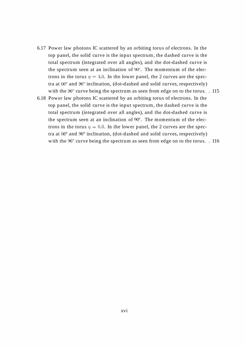
6.17 Power law photons IC scattered by an orbiting torus of electrons. In thetop panel, the solid curve is the input spectrum, the dashed curve is thetotal spectrum (integrated over all angles), and the dot-dashed curve isthe spectrum seen at an inclination of 90�. The momentum of the elec-trons in the torus � = 3:0. In the lower panel, the 2 curves are the spec-tra at 60� and 90� inclination, (dot-dashed and solid curves, respectively)with the 90� curve being the spectrum as seen from edge on to the torus. . 115

6.18 Power law photons IC scattered by an orbiting torus of electrons. In thetop panel, the solid curve is the input spectrum, the dashed curve is thetotal spectrum (integrated over all angles), and the dot-dashed curve isthe spectrum seen at an inclination of 90�. The momentum of the elec-trons in the torus � = 6:0. In the lower panel, the 2 curves are the spec-tra at 60� and 90� inclination, (dot-dashed and solid curves, respectively)with the 90� curve being the spectrum as seen from edge on to the torus. . 116

xvi

Part I

Background

1

Chapter 1

Theory of Compton scattering

This thesis investigates the Comptonization process within various physical contexts inhigh energy astrophysics. This Chapter gives an introduction to some of the main re-sults of Comptonization theory, and to astrophysical systems in which Comptonizationis important.

1.1 Introduction

Astrophysical sources of X-ray photons are frequently interpreted in terms of low en-ergy photons entering a region of hot plasma and scattering off energetic electrons. Thephotons gain energy (on average) from the electrons via the inverse Compton scatter-ing process. Energy exchange due to multiple inverse Compton scattering events istermed Comptonization. Photons may scatter multiple times, and before escaping fromthe plasma a typical photon may have been scattered up to X-ray or even gamma-rayenergies. Thus one is interested in the transport of photons through an electron plasmaas they gain energy at a succession of scattering events. Spectra given by this processare said to have been Comptonized.

1.2 Compton scattering

1.2.1 Energy shift

In the limit of a photon’s energy � being significantly smaller than the electron rest massenergy 511 keV, the interaction between a photon and an electron can be adequately

2

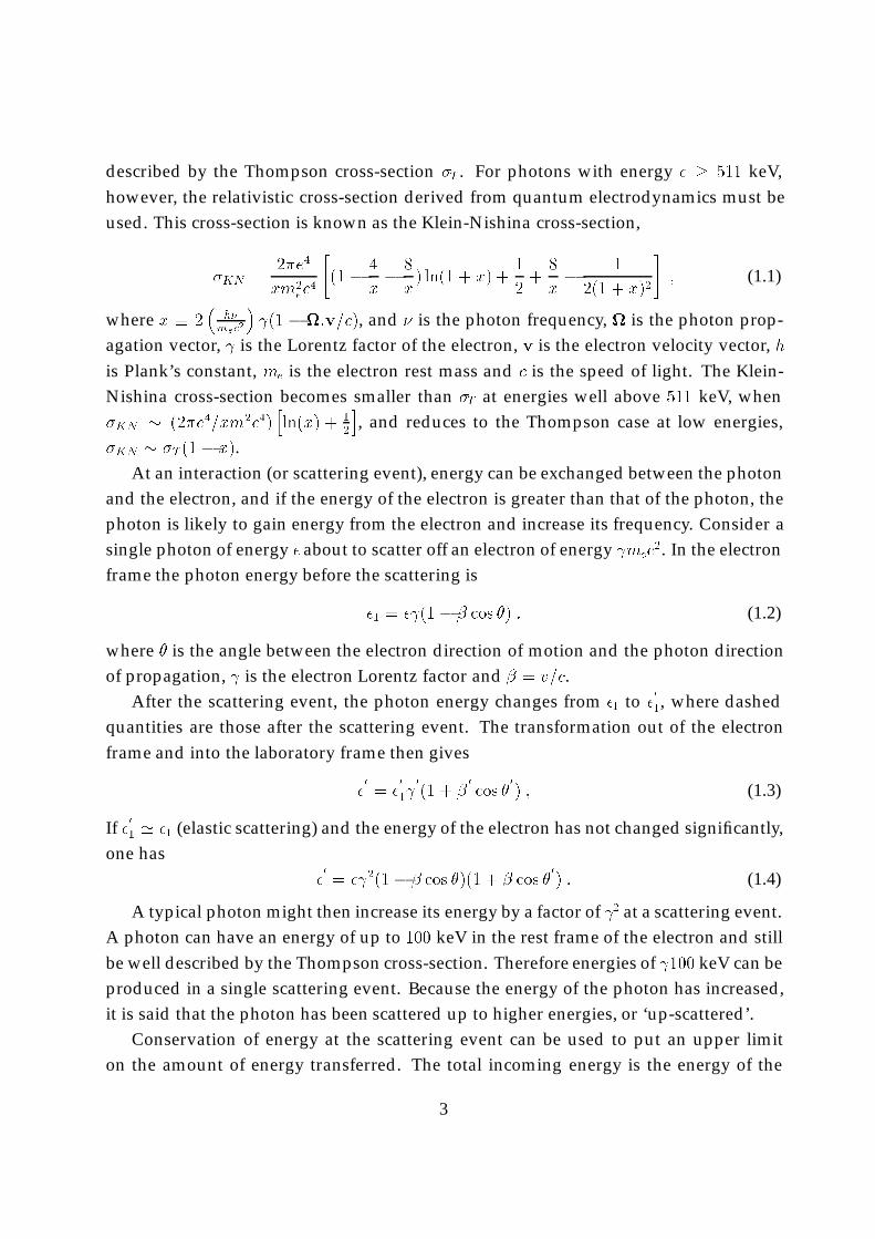
described by the Thompson cross-section �T . For photons with energy � � 511 keV,however, the relativistic cross-section derived from quantum electrodynamics must beused. This cross-section is known as the Klein-Nishina cross-section,

�KN =2�e4

xm2ec

4

"(1 � 4

x� 8

x) ln(1 + x) +

1

2+

8

x� 1

2(1 + x)2

#; (1.1)

where x � 2�

h�mec2

� (1 � :v=c), and � is the photon frequency, is the photon prop-

agation vector, is the Lorentz factor of the electron, v is the electron velocity vector, his Plank’s constant, me is the electron rest mass and c is the speed of light. The Klein-Nishina cross-section becomes smaller than �T at energies well above 511 keV, when�KN � (2�e4=xm2c4)

hln(x) + 1

2

i, and reduces to the Thompson case at low energies,

�KN � �T (1 � x).At an interaction (or scattering event), energy can be exchanged between the photon

and the electron, and if the energy of the electron is greater than that of the photon, thephoton is likely to gain energy from the electron and increase its frequency. Consider asingle photon of energy � about to scatter off an electron of energy mec

2. In the electronframe the photon energy before the scattering is

�1 = � (1� � cos �) : (1.2)

where � is the angle between the electron direction of motion and the photon directionof propagation, is the electron Lorentz factor and � = v=c.

After the scattering event, the photon energy changes from �1 to �0

1, where dashedquantities are those after the scattering event. The transformation out of the electronframe and into the laboratory frame then gives

�0

= �0

1 0

(1 + �0

cos �0

) ; (1.3)

If �0

1 ' �1 (elastic scattering) and the energy of the electron has not changed significantly,one has

�0

= � 2(1� � cos �)(1 + � cos �0

) : (1.4)

A typical photon might then increase its energy by a factor of 2 at a scattering event.A photon can have an energy of up to 100 keV in the rest frame of the electron and stillbe well described by the Thompson cross-section. Therefore energies of 100 keV can beproduced in a single scattering event. Because the energy of the photon has increased,it is said that the photon has been scattered up to higher energies, or ‘up-scattered’.

Conservation of energy at the scattering event can be used to put an upper limiton the amount of energy transferred. The total incoming energy is the energy of the

3

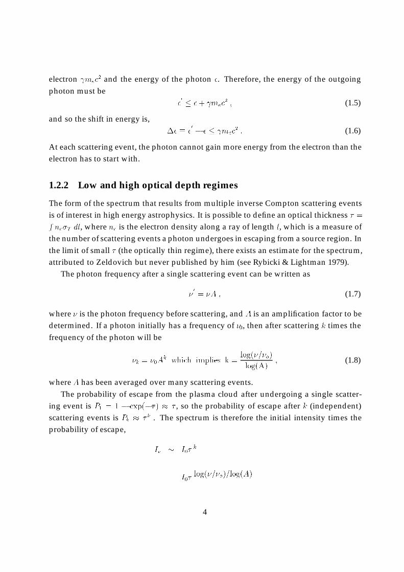
electron mec2 and the energy of the photon �. Therefore, the energy of the outgoing

photon must be�

0 � �+ mec2 ; (1.5)

and so the shift in energy is,�� � �

0 � � � mec2 : (1.6)

At each scattering event, the photon cannot gain more energy from the electron than theelectron has to start with.

1.2.2 Low and high optical depth regimes

The form of the spectrum that results from multiple inverse Compton scattering eventsis of interest in high energy astrophysics. It is possible to define an optical thickness � =Rne�T dl, where ne is the electron density along a ray of length l, which is a measure of

the number of scattering events a photon undergoes in escaping from a source region. Inthe limit of small � (the optically thin regime), there exists an estimate for the spectrum,attributed to Zeldovich but never published by him (see Rybicki & Lightman 1979).

The photon frequency after a single scattering event can be written as

�0

= �A ; (1.7)

where � is the photon frequency before scattering, and A is an amplification factor to bedetermined. If a photon initially has a frequency of �0, then after scattering k times thefrequency of the photon will be

�k = �0Ak which implies k =

log(�=�o)

log(A); (1.8)

where A has been averaged over many scattering events.The probability of escape from the plasma cloud after undergoing a single scatter-

ing event is P1 = 1 � exp(�� ) � � , so the probability of escape after k (independent)scattering events is Pk � � k . The spectrum is therefore the initial intensity times theprobability of escape,

I� � I0�k

= I0�log(�=�o)=log(A)

4

= I0

��

�0

�log(� )= log(A)

= I0

��

�0

���; (1.9)

where � � � log(� )= log(A). The spectrum from an optically thin electron cloud is there-fore a power law with energy spectral index �. Note that it has been implicitly assumedthat the amplification factor is not a function of photon frequency.

In the limit of infinite � (the infinitely optically thick case), and for non-relativistictemperatures, the evolution of the photon spectrum is determined by the Kompaneetsequation,

@ n(x; t)

@t= ne�T c�

1

x2@

@x

"x4 @ n(x; t)

@x+ n(x; t) + n(x; t)2

!#; (1.10)

where n(x; t) is the photon occupation number, x � h�=kTe is the dimensionless photonfrequency, and c the speed of light. � � kTe=mec

2 is the dimensionless electron temper-ature, with Te the electron temperature. The electron density ne is assumed constant.

The Kompaneets equation is a Fokker-Planck equation for the photon occupationnumber, that is found by expanding the Boltzmann equation in terms of a small energyshift at each scattering event. The first term in the curved brackets represents a seculargain of energy by the photons due to the Doppler effect, the second term is due tothe electron recoil effect and acts to limit the photon energy gain as the energy of thephotons approaches that of the electrons. The n(x; t)2 term describes induced scattering,a quantum effect that is usually negligible in most astrophysical applications.

The Kompaneets equation assumes that all the photons are of low enough energyto be described by the Thompson cross-section, and the electrons are non-relativistic sothat the average change in photon energy at a scattering event is small.

Dropping the n(x; t) and n(x; t)2 terms and changing variables gives

@ n(x; y)

@y=

1

x2@

@x

"x4 @ n(x; y)

@x

!#: (1.11)

where the Kompaneets y parameter is defined by y � ne�T c� t. (For a stationary casethe y parameter is defined as the product �� , and is a measure of the total amount ofenergy transferred from the electrons to the photons.)

Making a change of variables to x = exp(r) in Eq. 1.11 (so that @@x

= exp(�r) @@r

) gives

@ n

@y= 3

@ n

@r+@2 n

@r2: (1.12)

5

This equation is related to the one-dimensional diffusion equation by a further changeof variables. To see this, begin with the diffusion equation

@ n(z; s)

@s=

@2 n(z; s)

@z2; (1.13)

and change the variables from z and s to r and y, where

r = z � 3s (1.14)

y = s : (1.15)

By the chain rule, one has

@ n

@s=

@ n

@r

@ r

@s+@ n

@y

@ y

@s

= �3@ n@r

+@ n

@y; (1.16)

since @ r=@s = �3 and @ y=@s = 1. Also by the chain rule,

@ n

@z=

@ n

@r

@ r

@z+@ n

@y

@ y

@z

=@ n

@r; (1.17)

as @ r=@z = 1 and @ y=@z = 0. Eq. 1.17 then implies

@2 n

@z2=

@2 n

@r2: (1.18)

Substituting Eq. 1.16 and Eq. 1.18 into the diffusion equation 1.13 gives

@ n

@y= 3

@ n

@r+@2 n

@r2; (1.19)

which is the same as Eq. 1.12.The solution of the one-dimensional diffusion equation for an infinite medium is

given by

n(z; s) =1p4�s

Z1

�1

n0(z0) exp

(�(z � z0)2

4s

)dz0 ; (1.20)

where n0(z0) is the initial distribution when s = 0. With the change of variables z = 3y+r

and r = ln(x) the solution becomes

n(x; y) =1p4�y

Z1

�1

n0(z0) exp

(�(ln(x) + 3y � z0)2

4y

)dz0 ; (1.21)

6

where z0 = ln(x0). This solution to Kompaneets’ equation was first obtained by Zel-dovich & Sunyaev (1969).

For a monochromatic injection of photons this has a Gaussian profile that spreads out(broadens) in frequency with time, with the peak of the distribution moving to higherenergies.

1.2.3 Moderate optical depth regime

Sunyaev & Titarchuk (1980) have developed a means of using the solution (Eq. 1.21)to calculate the spectrum from a medium of finite extent and therefore finite opticalthickness (see also Illarionov, Kallman, McCray & Ross 1979).

Consider the injection of a certain number of photons into an electron plasma, wherethe energy of the photons is small compared to that of the electrons, and the electronsare non-relativistic so that the Thompson cross-section applies. Assume also that theplasma has a semi-infinite slab geometry. The solution to the infinite problem Eq. 1.21gives the energy of the photons after some time t. The method used by Sunyaev &Titarchuk (1980) is the following; if one knew how many of the photons had escapedfrom the slab between time t and t + dt, that is, the distribution of photons over theescape time from the slab, one could convolve this with Eq. 1.21 and determine thespectrum of escaping photons.

To find the distribution of photons over the escape time, Sunyaev and Titarchuksolved a spatial diffusion equation. Therefore, this technique relies on a double diffu-sion approximation: diffusion in space and diffusion in frequency (Eq. 1.13).

To investigate the spatial transport of photons in the slab, consider the one dimen-sional diffusion equation

@I(�; u)

@u=

1

3

@2I(�; u)

@� 2; (1.22)

where u � y=� is a dimensionless time parameter and � � ne�T r where the variable rmeasures the distance from the slab mid-plane. I is the angle-averaged intensity, wherethe photon occupation number is related to the intensity I by I � b nx3. Let us alsoassume that one face of the slab is along the plane � = 0 and the other face is at � = 2�0

where �0 � ne�Th, with h the half-thickness of the slab.The equation (Eq. 1.22) is separable, so if one looks for solutions of the formX(� )R(u)

one obtains

I(�; u) =1Xn=1

cnXn(� ) exp

(�(�n)2

3u

): (1.23)

7

In general, the boundary condition of the problem is used to determine the separationconstant �n, while the initial distribution n(x; 0) is used to determine the coefficients cn.For an arbitrary injection of photons, there may be infinitely many terms in the seriessolution Eq. 1.23. However, because �n increases with n, after some time the higherterms or modes will have died away compared to the first term or ‘fundamental’ mode.Therefore, the spatial distribution of photons approaches the distribution given by thefirst eigenfunction X1(� ) of the spatial equation. That is, at ‘late times’ one has

I(�; u)! c1X1(� ) exp(��u) ; (1.24)

where � � (�1)2=3.The distribution of photons over the escape time is simply the intensity at the bound-

ary of the slab as a function of time u, and this can be given by Eq. 1.24. A normalisationcondition is also required for the fraction of photons that have escaped. Using Eq. 1.24,

P (u) � I(0; u)R1

0 I(0; u) du

=c1X1(0) exp(��u)

c1X1(0)=�

= � exp(��u) : (1.25)

This function P (u) is the required distribution of photons over the escape time. Asdiscussed above, if the function P (u) is known it can be convolved with the solution toKompaneets’ equation to give the spectrum from a plasma cloud of finite extent,

N(x) =Z1

0n(x; u)P (u) du : (1.26)

Therefore the parameter � must be determined. This is done by appealing to the bound-ary condition of the problem.

Consider the spatial part of the problem. One has the equation

X00

n (� ) + �2nXn(� ) = 0 ; (1.27)

which has the orthogonal solutions

Xn = cos[�n(�o � � )] + sin[�n(�o � � )] : (1.28)

If one appeals to symmetry about the mid-plane of the disk and discards the sin solution,

8

Xn = cos[�n(�o � � )] : (1.29)

This equation is then used with the boundary condition to give �n (or equivalently �).The boundary condition from diffusion theory is (Zweifel 1973)

I

2= �D@I

@�: (1.30)

where the diffusion constant D in this case equals 1=3, from Eq. 1.22. This boundarycondition says that the number of escaping photons (the right hand side) is equal tohalf of the number of photons at the boundary (the left hand side). Presumably theother half of the photons are directed back into the cloud due to the assumed isotropyof the photon distribution.

It has been said that this condition holds that no photons are incident on the cloudfrom the outside. However, diffusion theory speaks only of the nett flow of particles(i.e. photons). Therefore, this condition says that there is no nett influx of photons fromoutside the cloud. Within the framework of diffusion theory, this is the best that can bedone.

In practice, even this boundary condition presents difficulties. An easier approachbegins by considering the linear extrapolation

I(� ) = I(0)(1� k� ) : (1.31)

Substituting this into the boundary condition (1.30) and solving for k gives k = 3=2. Sothe flux outside the surface of the cloud can be taken to obey

I(� ) = I(0)(1� (3=2)� ) : (1.32)

This says that the intensity goes to zero at a distance � = 2=3 outside the boundary. Thisgives a new and simple boundary condition: evaluate the intensity at this point outsidethe boundary (the so-called extrapolated length) and set it equal to zero. Doing this, onehas

Xn(�2=3) = 0) cos[�n(�o + 2=3)] = 0 ; (1.33)

so

�n =(2n � 1)�

2(�o + 2=3)) � =

�213

=�2

12(�o + 2=3)2: (1.34)

Now that � is known, everything about the distribution of photons over the escapetime P (u) is known. It is also seen that the spatial transport depends only on the opticaldepth �o.

This analysis can be repeated for spherical and cylindrical geometries, the principledifference being that the value of � (obtained from the boundary condition) is different.

9

1.2.4 The stationary equation

Knowing the distribution of photons over the escape time, and given Eq. 1.26, the spec-trum from a finite cloud can be found by performing the integration. However, moreinsight can be gained by using the same equations to derive another equation for thespectrum of a finite cloud, one that is stationary in time.

Begin with the Kompaneets equation Eq. 1.10. It is possible to construct an equationfor the time-independent spectrum N(x)

N(x) =Z1

0n(x; u)P (u) du : (1.35)

by substituting both the Kompaneets expression for n(x; u) and the equation for P (u),Eq. 1.25.

Dropping the n(x; u)2 term in Kompaneets’ equation, multiplying each side by P (u)

and then integrating gives

Z1

0�@ n

@uexp(��u) du =

�

x2@

@xx4(Z

1

0�n exp(��u) du + @

@x

Z1

0�n exp(��u) du

)

=�

x2@

@x

"x4 @ N(x)

@x+N(x)

!#: (1.36)

The left hand side equals

[�n exp(��u)]10 +Z1

0�2n exp(��u) du

= 0 � �n(x; 0) + �N(x)

= ��f(x)

x3+ �N(x) : (1.37)

where f(x) is a source that is equal to n(x; 0)x3. So the equation becomes

1

x2@

@x

"x4 @ N(x)

@x+N(x)

!#= N(x)�

f(x)

x3: (1.38)

where � �=�.The left hand side is identical to the Kompaneets equation. The first term on the right

hand side describes the escape of photons from the plasma cloud, while the second termdescribes the injection of photons due to a source f(x). The value of is given by thespatial diffusion problem.

10

By looking for a power law solution to the stationary equation of the form

N(x) = ax�(�+3) : (1.39)

it is found that

�(� + 3) = =�2

12�(�o + 2=3)2: (1.40)

for a slab geometry (using the value of � found earlier).This quadratic equation can be solved to give

� = �3

2�vuut9

4+

�2

12�(�o + 2=3)2: (1.41)

This equation relates the energy spectral index � to the temperature and optical depth ofthe cloud. The spectrum produced by inverse Compton scattering depends only on theelectron temperature and optical depth. It is also seen that the spectral slope is inverselyproportional to � and �o.

1.2.5 Spectral characteristics

Here the origin of the power law should be clarified. Where does the power law comefrom? What stops the energy gain from continuing indefinitely?

Consider again Kompaneets’ equation with the n(x; y)2 term neglected,

@ n(x; y)

@y=

1

x2@

@x

"x4 @ n(x; y)

@x+ n(x; y)

!#: (1.42)

Kompaneets’ equation can be used to investigate the rate of energy exchange betweenphotons and electrons, including both Doppler and recoil terms. Recall that the photonoccupation number is related to the intensity I by the formula I = b nx3, and the totalenergy of the photons can be obtained by integrating over the intensity. The rate ofenergy exchange is therefore

1

b

dE

dy=

d

dy

Z1

0n(x; u)x3 dx =

Z1

0

d n(x; u)

dyx3 dx : (1.43)

Substituting Kompaneets’ equation for dn(x; u)=dy (and ignoring any distinction be-tween partial and total derivatives) gives

1

b

dE

dy=

Z1

0x@

@x

"x4 @ n(x; y)

@x+ n(x; y)

!#dx

=Z1

0x@

@x

"x4

@ n

@x

#dx+

Z1

0x@

@x

hx4 n

idx ; (1.44)

11

Integrating both terms by parts (twice on the first term), and discarding the boundaryterms (because n is taken to be zero at x = 0; 1) one has

1

b

dE

dy= 4

Z1

0

hx3 n

idx�

Z1

0

hx4 n

idx : (1.45)

For small x, the first term dominates and a first order differential equation for Eresults

dE

dy= 4E ) E = E0 exp (4 y) : (1.46)

The gain of energy by the photons from the electrons increases exponentially with time(because y depends linearly on t).

For photons at higher frequencies the second (recoil) term becomes comparable withthe first (Doppler) term. To see this, consider those photons at a frequency of x = 4, thatis, put n = n0 �(x� 4) into the above expression. This gives

dE

dy= 4n0 (4)

3 � n0 (4)4 = 0 : (1.47)

That is, no nett energy is transferred to these photons. The Doppler term balances therecoil term. For photons at still higher energies the recoil effect dominates and photonslose energy.

It is seen that for inverse Compton scattering in an infinite medium, no power lawis formed (Eq. 1.21). In a medium of finite extent, however, the exponential increase ofthe photon’s energy can be balanced by the rate of escape from the cloud (for instance,the � exp (��u) function for the distribution of photons over their time of escape fromthe cloud). This balancing act forms a power law.

The power law does not extend indefinitely in energy, however. As a photon’s en-ergy approaches the energy of the scattering electrons the recoil effect becomes impor-tant and limits the amount of energy exchanged, until a photon at x = 4 experiences nonett gain or loss of energy. A cutoff in the spectrum is therefore produced by the recoileffect when the energy of the photons is approximately the same as the energy of theelectrons � kTe.

1.3 Compton scattering in astrophysical objects

Astrophysical systems in which Comptonization is an important process include radio-quiet active galactic nuclei, galactic black hole candidates, and magnetised compactstars. These are discussed below.

12

1.3.1 Disk-corona systems

Active galactic nuclei (AGN) are sources of X-rays and gamma-rays. The standard pic-ture for explaining the required energy release is the accretion of material onto a cen-tral supermassive black hole. Accretion is capable of liberating on the order of 10%of the rest-mass energy of the accreting material, and therefore can in principle provideenough power to account for the high energy emission. The accreting material will haveangular momentum and therefore will most probably form an accretion disk.

Assuming the accretion energy at a distance r in the disk is dissipated locally, andthat the disk is optically thick, the local disk emission will be blackbody (Peterson1997). Equating the luminosity per unit area of a blackbody sphere of radius r withthe Stefan-Boltzmann law �T4 gives an estimate for the local blackbody temperature,Tbb = (L=4�r2�)

1=4 ' 2�105 (L=LEdd)1=4(r=10rg)�1=2(M=107M�)�1=4K, where LEdd is theEddington luminosity, M� is the mass of the Sun, M is the mass of the black hole, rg isthe gravitational radius and � is the Stefan-Boltzmann constant. Thus accretion disks inAGN are a source of optical/UV photons, but are incapable of generating radiation athigher energies through blackbody emission.

In order to explain the observed X-ray emission in AGN spectra, it is necessary topostulate the existence of hot plasma located in the innermost regions of the accretiondisk. This hot plasma is typically referred to as a corona (Haardt & Maraschi 1991). Themost direct evidence for disk-coronae comes from galactic black hole systems that areapproximately edge on to our line of sight: when an eclipse occurs some X-ray flux isstill observed. This is interpreted as being due to material above and below the plane ofthe system scattering X-rays into our line-of-sight.

It is suggested (Liang 1979) that coronae in accreting compact systems cool primarilyvia the Comptonization process, with the low energy ‘soft’ photons being Comptonizedin the hot corona. The soft photons are emitted by the optically thick accretion disk,and thus have a blackbody distribution. The Comptonized photons form a power law(Section 1.2).

Seyfert galaxies are radio-quiet AGN whose X-ray spectra typically consist of a powerlaw I� / ��� with � � 1. Observationally, � is known to be almost constant. A con-stant � in Eq. 1.40 then implies the existence of some feedback mechanism between theelectron temperature and optical depth. If the temperature � were to increase (say), thevalue of the optical depth � must decrease correspondingly if � is to remain constant.Determining the nature of the feedback mechanism is the focus of two-phase disk-coronamodels (Haardt & Maraschi 1991), where for a given optical depth the temperature is

13

regulated by photon interaction between the cloud and an accretion disk.A number of possibilities exist for the geometry of the accretion disk corona in these

systems. One possibility is slab-like region located above and below the disk or someportion of the disk. Alternatively, there may be many ‘active regions’ heated by mag-netic fields, which would be distributed over the surface of the disk. The optical depth �

within the corona or active region is thought to be between 10�3�1 with the temperaturebeing in the range of a few hundred keV.

1.3.2 Galactic black hole candidates

In the case of galactic black hole candidates (BHCs), two stars orbit about each other,one of which is a compact object. The two types of galactic black hole candidates thatcan occur are the wind fed system, where material outflowing from the companion staris captured and accreted by the compact object, and the Roche-lobe filling system wherethe companion is an evolved star (Lewin, van Paradijs & van den Heuvel 1996). Materialfrom the evolved star is transferred to the compact companion by Roche lobe over-flow.In either case the accreting material will have angular momentum, and therefore willform an accretion disk.

The X-ray spectra observed from galactic black hole candidates can be classified intotwo main states, referred to as a soft state and a hard state (Tanaka & Lewin 1996). Thesoft state continuum spectrum consists of at least two components; a thermal compo-nent with a temperature of the order of 1 keV, and a power law with an energy spectralindex � that falls within the range 1:2 � 1:7, while the hard state consists of a singleextended power law with a spectral index in the range 0:4� 0:9 (Esin et al. 1998).

The power law spectra are attributed to Comptonization; however the geometryof the Comptonizing plasma is not well understood. The favoured geometry consistsof a hot spherical or quasi-spherical region in the central part of the accretion flow (the’hot’ solution of Eardley, Lightman & Shapiro 1975). The mechanism heating the coronalelectrons is also not definitively known. However, the electron distribution is most oftenmodeled as being a relativistic Maxwellian distribution of temperature of the order of100 keV, with an optical depth � of a few.

1.3.3 Accreting magnetic compact stars

Magnetised white dwarf and neutron stars may accrete material that has overflowed theRoche lobe of a companion star. The accreting (ionised) material is then channeled by

14

the magnetic field lines of the compact star into an accretion column above the magneticpole.

Electrons are heated at a standing shock formed near the base of the accretion col-umn, while the radiative cooling of the post-shock electrons is usually considered to bedominated by Bremsstrahlung emission. It is expected that the accretion column willcontain both temperature, velocity and density gradients in the post-shock region, asmaterial settles onto the surface of the star.

The hot post-shock material can emit the observed iron K� and K� lines (Fujimoto& Ishida 1997). It is possible for the accretion column to be optically thick to Comptonscattering of these line photons, especially within the post-shock region.

1.4 Thesis outline

The outline of this thesis is as follows. Chapter 2 discusses a linear Monte Carlo (MC)numerical technique. Chapter 3 presents a non-linear Monte Carlo code and a methodof extending the algorithm to account for density variations. Chapter 4 is an investiga-tion of a two-phase disk-corona model. The linear MC approach is used in Chapter 5 toinvestigate the time-lags due to Comptonization through a possible coronal geometryfor Cyg X-1. Chapter 6 applies the modified non-linear code to a study of Comptoniza-tion in bulk accretion flows; in a white dwarf accretion column where the electron den-sity, temperature and velocity are all functions of position in the column, and in a torusof material orbiting around some compact object.

15

References

Eardley, D. M., Lightman, A. P. & Shapiro, S. l. 1975, ApJ, 199, L153Esin, A. A., et al. 1998, ApJ, 505, 854Fujimoto, R. & Ishida, M. 1997, ApJ, 474, 774Haardt, F. & Maraschi, L. 1991, ApJ, 380, L51Illarionov, A., Kallman, T., McCray, R., & Ross, R. 1979, ApJ, 228, 279Liang, E. P. T. 1979, ApJ, 231, L111Peterson, B. M. 1997, “An Introduction to Active Galactic Nuclei”, (Cambridge Univ.

Press)Rybicki, G. B. & Lightman, A. P. 1979, “Radiative Processes in Astrophysics”, (New

York: Wiley)Sunyaev, R. A. & Titarchuk, L. G. 1980, A&A, 86, 121Tanaka, Y., Lewin, W. H. G. 1996, “X-Ray Binaries”, eds. W. H. G. Lewin, J. van Paradijs

& E. P. J. van den Heuvel (Cambridge Univ. Press.)Zeldovich, YA. B. & Sunyaev, R. A. 1969, Ap.& Space Sci., 4, 301Zweifel, P. F. 1973, “Reactor Physics”, (New York: McGraw-Hill)

16

Part II

Technical

17

Chapter 2

Monte Carlo numerical approach

Comptonization in astrophysical systems is frequently treated using the Monte Carlomethod. This Chapter presents an introduction to the numerical techniques used inlinear Monte Carlo photon transport codes.

2.1 Monte Carlo photon transport

The diffusion approach discussed in Chapter 1 is limited in a number of ways. Theenergy diffusion assumption does not hold in most plasmas of astrophysical interest,because the photon energy changes by a large amount at a scattering event. In rarefiedplasmas, the distance between scattering events can be large, so the spatial diffusionapproximation is also a poor one. In addition, the mean free path of the photons is afunction of photon energy as well as plasma density, which also complicates the spatialtransport. The situation is further complicated if the geometry of the plasma is nottrivial, if other processes (such as absorption) are taken into account, and if complicatedphoton source functions are to be investigated. Spectra that are formed by this processare therefore more easily calculated using numerical or semi-analytic techniques.

Semi-analytic approaches include the radiative transfer approach (Nagirner & Pouta-nen 1993) and the kinetic equation approach (Coppi 1992). Of the numerical approaches,the most commonly used is the Monte Carlo technique (MacKeown 1997) for simulatingthe transport of photons through a plasma. An advantage of using Monte Carlo simu-lations is their flexibility; these codes can be easily modified to be applicable to manyastrophysical settings.

Most Monte Carlo simulations of inverse Compton scattering are ‘analogue’ simula-

18

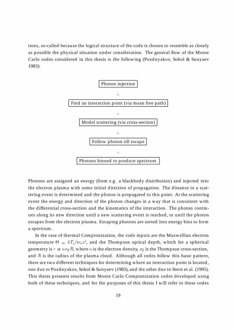
tions, so-called because the logical structure of the code is chosen to resemble as closelyas possible the physical situation under consideration. The general flow of the MonteCarlo codes considered in this thesis is the following (Pozdnyakov, Sobol & Sunyaev1983):

Photon injection

#Find an interaction point (via mean free path)

#Model scattering (via cross-section)

#Follow photon till escape

#Photons binned to produce spectrum.

Photons are assigned an energy (from e.g. a blackbody distribution) and injected intothe electron plasma with some initial direction of propagation. The distance to a scat-tering event is determined and the photon is propagated to this point. At the scatteringevent the energy and direction of the photon changes in a way that is consistent withthe differential cross-section and the kinematics of the interaction. The photon contin-ues along its new direction until a new scattering event is reached, or until the photonescapes from the electron plasma. Escaping photons are sorted into energy bins to forma spectrum.

In the case of thermal Comptonization, the code inputs are the Maxwellian electrontemperature � � kTe=mec

2, and the Thompson optical depth, which for a sphericalgeometry is � � n�TR, where n is the electron density, �T is the Thompson cross-section,and R is the radius of the plasma cloud. Although all codes follow this basic pattern,there are two different techniques for determining where an interaction point is located,one due to Pozdnyakov, Sobol & Sunyaev (1983), and the other due to Stern et al. (1995).This thesis presents results from Monte Carlo Comptonization codes developed usingboth of these techniques, and for the purposes of this thesis I will refer to these codes

19

as ‘linear’ and ‘non-linear’ respectively (even when the ‘non-linear’ code is being usedin a ‘linear’ mode). Each code was written using algorithms published in Pozdnyakov,Sobol & Sunyaev (1983) and Stern et al. (1995). Other papers discussing the algorithmsused for inverse Compton simulations are G�orecki & Wilczewski (1984), and Hua (1997).

Below an introduction to the basic Monte Carlo method is given, then the method formodeling electron-photon scattering events is presented in Section 2.1.3. The methodof transporting photons through the simulation is discussed in Section 2.1.4. The em-phasis in this Chapter is on the methods behind linear Monte Carlo codes, although themodeling of the actual scattering events uses the same algorithm for both the linear andnon-linear approaches.

2.1.1 Introduction to the Monte Carlo technique

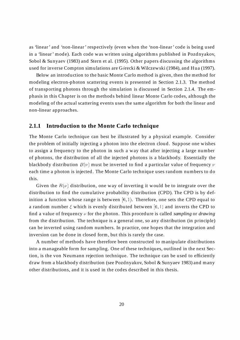
The Monte Carlo technique can best be illustrated by a physical example. Considerthe problem of initially injecting a photon into the electron cloud. Suppose one wishesto assign a frequency to the photon in such a way that after injecting a large numberof photons, the distribution of all the injected photons is a blackbody. Essentially theblackbody distribution B(�) must be inverted to find a particular value of frequency �

each time a photon is injected. The Monte Carlo technique uses random numbers to dothis.

Given the B(�) distribution, one way of inverting it would be to integrate over thedistribution to find the cumulative probability distribution (CPD). The CPD is by def-inition a function whose range is between [0; 1). Therefore, one sets the CPD equal toa random number � which is evenly distributed between [0; 1) and inverts the CPD tofind a value of frequency � for the photon. This procedure is called sampling or drawingfrom the distribution. The technique is a general one, so any distribution (in principle)can be inverted using random numbers. In practice, one hopes that the integration andinversion can be done in closed form, but this is rarely the case.

A number of methods have therefore been constructed to manipulate distributionsinto a manageable form for sampling. One of these techniques, outlined in the next Sec-tion, is the von Neumann rejection technique. The technique can be used to efficientlydraw from a blackbody distribution (see Pozdnyakov, Sobol & Sunyaev 1983) and manyother distributions, and it is used in the codes described in this thesis.

20

E Sampled

Random

B (E)

E

B (E)

ProbabilityDistribution Cumulative

ProbabilityDistribution

Integrate

Figure 2.1: Illustration of the basic direct inversion Monte Carlo method

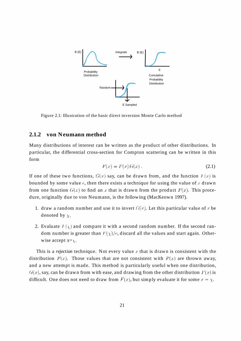
2.1.2 von Neumann method

Many distributions of interest can be written as the product of other distributions. Inparticular, the differential cross-section for Compton scattering can be written in thisform

P (x) = F (x)G(x) : (2.1)

If one of these two functions, G(x) say, can be drawn from, and the function F (x) isbounded by some value c, then there exists a technique for using the value of x drawnfrom one function G(x) to find an x that is drawn from the product P (x). This proce-dure, originally due to von Neumann, is the following (MacKeown 1997).

1. draw a random number and use it to invert G(x). Let this particular value of x bedenoted by �.

2. Evaluate F (�) and compare it with a second random number. If the second ran-dom number is greater than F (�)=c, discard all the values and start again. Other-wise accept x=�.

This is a rejection technique. Not every value x that is drawn is consistent with thedistribution P (x). Those values that are not consistent with P (x) are thrown away,and a new attempt is made. This method is particularly useful when one distribution,G(x), say, can be drawn from with ease, and drawing from the other distribution F (x) isdifficult. One does not need to draw from F (x), but simply evaluate it for some x = �.

21

2.1.3 Modeling a scattering event

Finding an electron

Pozdnyakov, Sobol & Sunyaev (1983) and G�orecki & Wilczewski (1984) have used thevon Neumann technique to sample from the distributions describing a scattering event.The following discussion outlines how this method is implemented in linear MonteCarlo codes.

Consider a photon propagating in some direction with some energy h�. First, anelectron must be found to interact with the photon. Therefore one needs to consider thedistribution of scattering electrons, which is of the form

�(x) (1�:v=c)N(p) ; (2.2)

where N(p) is the momentum distribution for the electrons, v is the direction of electronmotion, and �(x) is the cross-section with

x � 2

h�

mec2

! (1 �:v=c) ; (2.3)

where is the electron Lorentz factor and � is the photon frequency.In the case where the electron distribution N(p) is Maxwellian (N(p) � ne(p)), an

algorithm for sampling N(p) is known. It can also be shown that the pre-factor f(x) isbounded,

f(x) � �(x) (1�:v=c) � 2�(x) � 8=3 : (2.4)

Therefore, one can sample the Maxwellian distribution and then use the von Neumannmethod to sample the product Eq. 2.2. The method is

1. Draw a value for the electron momentum from N(p), and a direction of motion forthe electron from an isotropic distribution,

2. Use these values to evaluate f(x),

3. if a random number � is

� < (3=8) �(x) (1 �:v=c) ; (2.5)

then accept the electron momentum p and direction of motion v, else

4. reject the electron values and draw new values for the electron momentum anddirection.

22

The scattering event

Having found an electron to scatter with the photon, it is then necessary to find a newdirection of propagation and a new energy for the photon after the scattering event. Thisis done by sampling the Klein-Nishina differential scattering cross-section (see Chapter1).

The differential cross-section can be written as a product of the form

P (�;')Y (2.6)

whereP (�;') =

1

4� 2(1� �v=c)2; (2.7)

with � being the angle cosine between the electron and the photon and v the electronvelocity. The other part of the product has the following form

Y � x

0

x

!2

(x; x0

) ; (2.8)

(x; x0

) � x

x0+x

0

x+ 4

�1

x� 1

x0

�+ 4

�1

x� 1

x0

�2; (2.9)

with

x � 2

h�

mec2

! (1� �v=c) and x

0 � 2

h�

0

mec2

! (1� �

0

v=c) : (2.10)

The function Y is bounded (Y � 2), and can be evaluated easily if x and x0 are known.

The prime denotes quantities after scattering. The angular factor P (�;') can be inverteddirectly (Section 2.1.1) for the scattering angles:

� =v=c+ (2� � 1)

1 + (v=c)(2� � 1)(2.11)

' = 2��1 : (2.12)

where � and �1 are uniform random numbers on [0,1). Using these angles a new direc-tion of propagation

0 , and the cosine of the scattering angle :0 , can be computed.The function Y is then found by evaluating where

x0

x=

"1 +

h�(1 �:0

)

mec2(1 � �v=c)

#�1: (2.13)

The differential cross-section then consists of one part that can be sampled (P (�;'),Eq. 2.11 and Eq. 2.12), and another part (Y ) that is bounded and that can be evaluated

23

given the angles. Therefore the rejection test can be applied for sampling the differentialcross-section (Eq. 2.6). The procedure is

1. Draw from the angular factor P (�;') using Eq. 2.11 and Eq. 2.12, and use them tofind :

0

2. Use the parameters of the photon, the electron and :0 to compute Y .

3. If a random number 2�2 < Y then set = 0 , and the new energy of the photon is

E0

= x0

[2 (1 � �v=c)]�1mec2 ; (2.14)

else

4. reject the scattering event, draw another two angles � and', and try again withthe same electron.

2.1.4 The photon transport technique

In addition to modeling scattering events, the other key technique required for linearMonte Carlo simulations is a method for transporting the photons from one scatteringevent to the next. In a linear code, the following procedure is used.

The distance l to the next scattering point is determined by inverting the cumulativeprobability distribution

� = exp (�� ) � exp (�Z l

0n(s)� ds) ; (2.15)

where � is a uniform random number between zero and one and the cross-section � hasbeen averaged over the distribution of target electrons. For a constant density n(s) = n,the expression becomes

l = � 1

n�ln(�) : (2.16)

orl = �� ln(�) ; (2.17)

where � is the mean free path. In the linear simulation, the mean free path is determinedby averaging the cross-section over the Maxwellian electron momentum distributionne(p), which in spherical polar co-ordinates takes the form

� =4�R1

0 ne(p)p2 dp

2�neR1

0 ne(p)p2R 1�1 �KN(x)(1� �v=c) d� dp

(2.18)

24

(Pozdnyakov, Sobol & Sunyaev 1983) with x defined in Eq. 2.10. Given a photon prop-agating in a direction and with r being the current position of the photon in thesimulation, the new position r

0 of the photon is then

r0

= r+ l : (2.19)

This technique, while being very clear and obvious, is limited because the methodfor calculating the mean free path �, Eq. 2.18, has assumed the electron plasma is ho-mogeneous and isotropic. If bulk flows of electrons exist in the plasma, evaluating themean free path integral becomes more difficult (Janiuk, Czerny & Zycki 2000).

2.2 Summary

In this Chapter, the structure of linear Monte Carlo photon transport codes has beenreviewed, including an introduction to the basic Monte Carlo technique. Section 2.1.3gave a discussion of how scattering events are modeled, and Section 2.1.4 discussedhow a photon is transported through a plasma of constant density. Although the lin-ear Monte Carlo procedure as outlined in this Chapter is a flexible way of treating theComptonization problem, the next Chapter introduces (and modifies) the non-linearapproach to make the numerical method even more flexible.

25

References

Coppi, P. S. 1992, MNRAS, 258, 657G�orecki, A. & Wilczewski, W. 1984, Acta Astron., 34, 141Hua, X. 1997, Com. Ph. 11, 660 (physics/9709023)Janiuk, A., Czerny, B. & Zycki, P. T. 2000, MNRAS, 318, 180MacKeown, P. K. 1997, ”Stochastic Simulation in Physics”, (Springer-Verlag, Singapore)Nagirner, D. I. & Poutanen, J. 1993, A&A, 275, 325Pozdnyakov, L. A., Sobol, I. M. & Sunyaev, R. A. 1983, Ap.& Space Sci. Reviews, 2, 189Stern, B., et al. 1995, MNRAS, 272, 291

26

Chapter 3

Photon transport through plasmas withdensity and velocity structure

Linear Monte Carlo codes (Chapter 2) are typically applied to scattering in plasmaswithout temperature and density gradients. Treating bulk motion can be difficult evenfor simple cases. With the introduction into the field of algorithms associated with non-linear Monte Carlo (NLMC) codes, these problems are now more tractable numerically.NLMC can already handle arbitrary velocity structures in a plasma. Here the NLMCtechnique is discussed, and an extension of the algorithm is proposed that enables theeasy calculation of photon transport in plasmas with non-constant density as well asnon-constant temperature and/or bulk motion.

3.1 Overview

Monte Carlo simulations of photon scattering are analogue simulations. As discussedin the previous Chapter, after a photon of some energy is injected into the plasma, thelocation of the next scattering point is sampled using the mean free path. The scatteringevent is modeled by sampling the differential cross-section, and the new energy andnew direction is assigned to the photon. The photon is followed until it escapes theplasma. After following many photons a spectrum is generated. A weighting technique(see Section 3.4.1) is generally used to treat the spatial transport, whereby a weightedfraction of the photon is forced to scatter, while the rest of the photon escapes. Theweight function is determined at each scattering point by the probability of escape fromthe plasma (Molnar & Birkinshaw 1999). This is useful when the probability of a given

27

photon undergoing a scattering event is very small.A linear algorithm (Pozdnyakov, Sobol, & Sunyaev 1983) has been used to treat the

Comptonization problem in regions where the plasma has a well defined temperatureand a homogeneous density. However, astrophysical plasmas are often inhomogeneousand non-isothermal. Additionally, treating bulk motion of the plasma with such a codeis difficult even for simple cases.

By dividing the plasma into various zones, with each zone having a different tem-perature and density, temperature and density variations can be studied in a crude way,for instance, by having the density decrease in a series of steps. An improvement onthis situation was made by Hua (1997), who developed a code to treat smooth densityvariations; however the plasma was still required to be isothermal, and no bulk motionwas considered.

As an alternative, the non-linear algorithm was introduced by Stern et al. (1995).The main difference in this non-linear approach is the way the photons are transported,since this method uses a von Neumann rejection algorithm for finding the location of thenext scattering point. In the following Section the method of photon transport currentlyused by non-linear Monte Carlo methods is reviewed. Section 3.3 presents a method ofcombining the Hua and Stern algorithms that enables the treatment of smooth densityvariations in the presence of temperature variations and bulk motion. Sections 3.4 and3.5 discuss implementation of the modification and give examples of astrophysical ap-plications. Detailed discussions of how to model the actual scattering events have beengiven by Pozdnyakov, Sobol & Sunyaev (1983), Gorecki and Wilczewski (1984), Hua(1997), and in Chapter 2 of this thesis.

3.2 Non-linear Monte Carlo simulation

3.2.1 Conventional algorithm

A photon has a certain probability of interacting with each of the electrons around it.Each of these probabilities can be written as a partial interaction rate,

PiT =�

volVrel : (3.1)

where Vrel is the relative velocity between the photon and a given electron, vol is thevolume of the plasma-filled region, and � is the cross-section. The subscript i denotesthe incident particle, and the subscript T the target particle.

28

To find the total interaction rate, that is, the total number of scattering events persecond, one sums all the partial interaction rates,

Pi =XT

PiT : (3.2)

The time of flight to the next scattering event is then sampled with the expression

t = � ln(�)

Pi; (3.3)

where � is a random number uniformly distributed on [0; 1) (Chapter 2). This time canbe converted into the distance propagated l by including a factor of c. An electron ischosen to interact with the photon based on the partial interaction rates, and then thescattering event is simulated using the technique described previously in Section 2:1:3.

3.2.2 Current non-linear Monte Carlo method

Stern et al. (1995) proposed a technique that increases efficiency by making use of theconcept of a virtual cross-section (Woodcock et al. 1965, Nelson, Hirayama & Rogers1985). This technique enables the simulation of photon scattering by electrons in bulkflow.

The rate of scattering events for a beam of photons (where the beam consists of asingle photon, say) incident with a beam of electrons at some point is n�KNVrel, with n

the electron density at the point. This quantity, which is used to determine if a scatteringevent takes place, depends on the photon’s energy through the Klein-Nishina cross-section �KN, and the energy of the electrons through the relative velocity Vrel.

In the case of a photon interacting with electrons, the relativistic expression for scat-tering rate is (Landau & Lifshitz 1971)

�KNP1�P

�2

E1E2n (3.4)

where P1� is the momentum four-vector of particle 1, P�2 is the momentum four-vector

of particle 2, E1 and E2 are the energies of particles 1 and 2, �KN is the cross-section andn is the density of target particles, in this case electrons.

The four-vector contraction is P1�P�2 = E1E2 � p1p2 where p1 and p2 are the mo-

mentum vectors of the particles, and so

P1�P�2

E1E2=

E1E2 � p1p2

E1E2= (1� p1

E1:p2

E2) = (1�:v) (3.5)

29

where is the unit vector in the photon propagation direction and v is the electronvelocity vector, and units where c � 1 have been assumed. On comparison of Eq. (3.4)with n�KNVrel, one sees that correct scattering rates are obtained if the quantity (1�:v)is identified as Vrel.

The non-linear simulation is divided into a series of time steps, with multiple pho-tons being followed simultaneously (their parameters being stored in arrays). Withineach time step, and for each photon, the interaction rate (above) is used to sample thetime between scattering events (which must be smaller than the time step), rather thanthe distance (Eq. 2.16), with

t = � 1

n�KNVrelln(�) ; (3.6)

where n�Vrel is the rate of scattering events, and it has been assumed that all the elec-trons have the same Vrel. This is, of course, an approximation. Each electron has adifferent velocity Vrel relative to the photon. The real interaction rate (which for a com-plicated situation is difficult to evaluate) is the sum of all the partial interaction rates ofall the electrons in the plasma. One does not wish to sum over all the electrons in thesimulation, so the algorithm used by non-linear codes assumes the existence of a virtualprocess, such that

n(�KN + �virt)Vrel � n�T2c (3.7)

(Stern et al. 1995), where �virt is the cross-section of the virtual process and �T is theThompson cross-section. If scattering in regions of homogeneous density is to be con-sidered, n can be dropped from the above to give

(�KN + �virt)Vrel = �T2c : (3.8)

The purpose of introducing the virtual process is that the right hand side of Eq. 3.7 isan upper limit on the real interaction rate, and is constant along the photon’s path, so itis easy to use this value to sample the time to the next interaction event with

t = � 1

n�T2cln(�) : (3.9)

An electron for the photon to scatter with is then found. But, having used the RHS ofEq. 3.7, the virtual (unphysical) process or channel must be disregarded to determineif a real scattering event takes place. To put it another way, at each point along thetrajectory the probability of an interaction is the sum of the probability of the virtualprocess occurring, and the probability of the real process occurring. Therefore, the realscattering event (or channel) is accepted/selected with a probability (�KNVrel)=(�T 2c),

30

otherwise the event is rejected as being due to the virtual process, and the photon con-tinues without scattering until the next time step.

This rejection algorithm is efficient unless the electron is moving relativistically inthe same direction as the photon, in which case Vrel becomes small, and if the photonenergy is very large, in which case the cross-section �KN becomes small. The benefits ofsuch a procedure are

� it can be extended easily to include other processes,

� no integrals for determining the mean free path through the electrons are required,and

� because finding a tentative scattering point does not require any knowledge of thevelocity structure in the accretion flow, this algorithm can easily handle problemswhere there is bulk motion of the flow, as expected for accretion problems.

Figure 3.1 shows spectra that result when this procedure is implemented, in this casefor a homogeneous sphere of plasma with electron temperature 25 keV. Solid lines areoutput from the non-linear code and dotted lines from the linear code (see Chapter 2).Five different optical depths for the sphere are considered, 3, 4, 5, 7 and 10. The photonsthat are initially injected into the plasma are sampled from a blackbody distributionwith a temperature equivalent to 10�8mec

2. The results are consistent with the resultsobtained using the linear algorithm of Pozdnyakov, Sobol & Sunyaev (1983).

To use the NLMC method to treat bulk motion of the flow, first determine a (poten-tial) scattering point using n�T2c as the rate of scattering events (Eq. 3.7). One thendetermines the direction and momentum of the flow. This gives the relative velocityof the electron that is needed for the rejection test. One then calculates the real cross-section and accepts or rejects the scattering event using (�KNVrel)=(�T 2c). If the eventis rejected the photon continues on its way until the next time step. If studying an ac-cretion flow with a temperature gradient at the tentative scattering point, determinewhat the temperature is at this point, draw an electron from a distribution with thistemperature, and then decide to accept or reject the scattering event.

3.3 Refined algorithm

The previous section assumed an interaction rate n�T 2c that is constant along the pho-ton’s path, because the density is taken to be a constant. Hua (1997) described how a

31

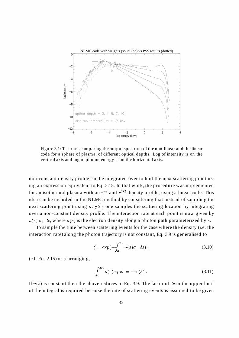
NLMC code with weights (solid line) vs PSS results (dotted)

-8 -6 -4 -2 0 2 4log energy (keV)

−12

−10

−8

−6

−4

−2

0

log

inte

nsity

Figure 3.1: Test runs comparing the output spectrum of the non-linear and the linearcode for a sphere of plasma, of different optical depths. Log of intensity is on thevertical axis and log of photon energy is on the horizontal axis.

non-constant density profile can be integrated over to find the next scattering point us-ing an expression equivalent to Eq. 2.15. In that work, the procedure was implementedfor an isothermal plasma with an r�1 and r3=2 density profile, using a linear code. Thisidea can be included in the NLMC method by considering that instead of sampling thenext scattering point using n�T 2c, one samples the scattering location by integratingover a non-constant density profile. The interaction rate at each point is now given byn(s) �T 2c, where n(s) is the electron density along a photon path parameterized by s.

To sample the time between scattering events for the case where the density (i.e. theinteraction rate) along the photon trajectory is not constant, Eq. 3.9 is generalised to

� = exp(�Z 2ct

0n(s)�T ds) ; (3.10)

(c.f. Eq. 2.15) or rearranging,Z 2ct

0n(s)�T ds = �ln(�) : (3.11)

If n(s) is constant then the above reduces to Eq. 3.9. The factor of 2c in the upper limitof the integral is required because the rate of scattering events is assumed to be given

32

by n(s)�T 2c. The distance to the next scattering point is then just the time multipliedby the speed of light.

The distance above can be thought of as an lower limit on how far the photon actu-ally travels, because it uses an upper limit on the interaction rate. In reality, the cross-section is not �T and the relative velocity is not 2c. So this scattering point is only‘tentative’.

Having found a tentative interaction point using the above method, the real interac-tion rate at the scattering point plus the virtual interaction rate is taken to be

n(s)(�KN + �virt)Vrel � n(s) �T 2c : (3.12)

So one accepts the tentative scattering event with probability

n(s) �KN Vreln(s) �T 2c

=�KN Vrel�T 2c

: (3.13)

This procedure is analogous to that described in the previous Section. Note that nointegral is required in Eq. 3.13 as the expression is evaluated at the (potential) scatteringpoint, not along the photon’s path (however the integral in Eq. 3.10 is along the photon’spath). To summarise the extended algorithm, a particular interaction rate (n(s)�T 2c)has been assumed to hold at all points along the photon’s path. This enables the distanceto the next scattering point to be sampled with ease (Eq. 3.11) using the Hua method.However, by assuming an interaction rate n(s)�T 2c, the number of scattering pointsalong a trajectory has been over-sampled. Some scattering points must be rejected togive a physical simulation. At each (potential) scattering point, the fraction of scatteringevents that are kept (accepted as being due to the physical cross-section) is given by Eq.3.13, with the rejected scattering points being due to the virtual cross-section.

The only difference between this proceedure and the conventional (Stern) algorithmis that one is now performing the distance integral explicitly, rather than using an ex-pression that can be integrated in closed form and inverted. This procedure is valid inthe relativistic limit and is exact: no approximations have been made.

3.4 Implementation of the method

This modified algorithm can still be used if photons are weighted in energy (in fact,this is often required for good spectral resolution, Stern et al. 1995). Note also that theefficiency of accepting a scattering event is independent of the density at that point, be-cause n(s) has canceled in Eq. 3.13. The integration over the density profile is now the

33

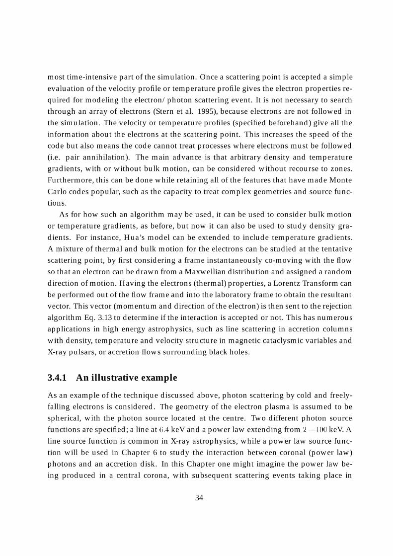
most time-intensive part of the simulation. Once a scattering point is accepted a simpleevaluation of the velocity profile or temperature profile gives the electron properties re-quired for modeling the electron/photon scattering event. It is not necessary to searchthrough an array of electrons (Stern et al. 1995), because electrons are not followed inthe simulation. The velocity or temperature profiles (specified beforehand) give all theinformation about the electrons at the scattering point. This increases the speed of thecode but also means the code cannot treat processes where electrons must be followed(i.e. pair annihilation). The main advance is that arbitrary density and temperaturegradients, with or without bulk motion, can be considered without recourse to zones.Furthermore, this can be done while retaining all of the features that have made MonteCarlo codes popular, such as the capacity to treat complex geometries and source func-tions.

As for how such an algorithm may be used, it can be used to consider bulk motionor temperature gradients, as before, but now it can also be used to study density gra-dients. For instance, Hua’s model can be extended to include temperature gradients.A mixture of thermal and bulk motion for the electrons can be studied at the tentativescattering point, by first considering a frame instantaneously co-moving with the flowso that an electron can be drawn from a Maxwellian distribution and assigned a randomdirection of motion. Having the electrons (thermal) properties, a Lorentz Transform canbe performed out of the flow frame and into the laboratory frame to obtain the resultantvector. This vector (momentum and direction of the electron) is then sent to the rejectionalgorithm Eq. 3.13 to determine if the interaction is accepted or not. This has numerousapplications in high energy astrophysics, such as line scattering in accretion columnswith density, temperature and velocity structure in magnetic cataclysmic variables andX-ray pulsars, or accretion flows surrounding black holes.

3.4.1 An illustrative example

As an example of the technique discussed above, photon scattering by cold and freely-falling electrons is considered. The geometry of the electron plasma is assumed to bespherical, with the photon source located at the centre. Two different photon sourcefunctions are specified; a line at 6:4 keV and a power law extending from 2� 100 keV. Aline source function is common in X-ray astrophysics, while a power law source func-tion will be used in Chapter 6 to study the interaction between coronal (power law)photons and an accretion disk. In this Chapter one might imagine the power law be-ing produced in a central corona, with subsequent scattering events taking place in

34

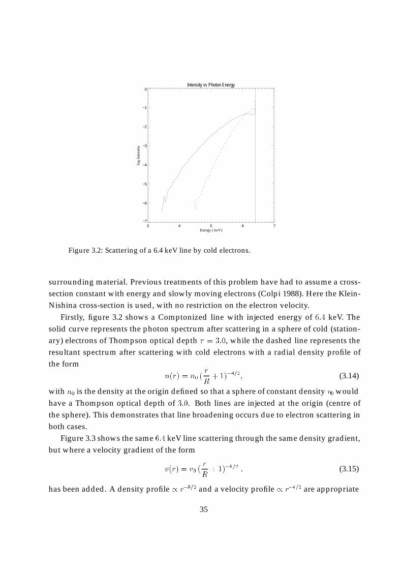
Intensity vs Photon Energy

3 4 5 6 7Energy ( keV)

−7

−6

−5

−4

−3

−2

−1

0

log

Inte

nsity

Figure 3.2: Scattering of a 6.4 keV line by cold electrons.

surrounding material. Previous treatments of this problem have had to assume a cross-section constant with energy and slowly moving electrons (Colpi 1988). Here the Klein-Nishina cross-section is used, with no restriction on the electron velocity.

Firstly, figure 3.2 shows a Comptonized line with injected energy of 6:4 keV. Thesolid curve represents the photon spectrum after scattering in a sphere of cold (station-ary) electrons of Thompson optical depth � = 3:0, while the dashed line represents theresultant spectrum after scattering with cold electrons with a radial density profile ofthe form

n(r) = n0 (r

R+ 1)�3=2; (3.14)

with n0 is the density at the origin defined so that a sphere of constant density n0 wouldhave a Thompson optical depth of 3:0. Both lines are injected at the origin (centre ofthe sphere). This demonstrates that line broadening occurs due to electron scattering inboth cases.

Figure 3.3 shows the same 6:4 keV line scattering through the same density gradient,but where a velocity gradient of the form

v(r) = v0 (r

R+ 1)�1=2 : (3.15)

has been added. A density profile / r�3=2 and a velocity profile / r�1=2 are appropriate

35

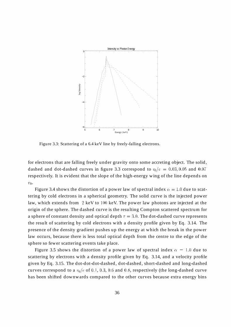
Intensity vs Photon Energy

5 6 7 8 9 10Energy ( keV)

−6

−4

−2

0

log

Inte

nsity

Figure 3.3: Scattering of a 6.4 keV line by freely-falling electrons.

for electrons that are falling freely under gravity onto some accreting object. The solid,dashed and dot-dashed curves in figure 3.3 correspond to v0=c = 0:03; 0:05 and 0:07

respectively. It is evident that the slope of the high-energy wing of the line depends onv0.

Figure 3.4 shows the distortion of a power law of spectral index � = 1:0 due to scat-tering by cold electrons in a spherical geometry. The solid curve is the injected powerlaw, which extends from 2 keV to 100 keV. The power law photons are injected at theorigin of the sphere. The dashed curve is the resulting Compton scattered spectrum fora sphere of constant density and optical depth � = 3:0. The dot-dashed curve representsthe result of scattering by cold electrons with a density profile given by Eq. 3.14. Thepresence of the density gradient pushes up the energy at which the break in the powerlaw occurs, because there is less total optical depth from the centre to the edge of thesphere so fewer scattering events take place.

Figure 3.5 shows the distortion of a power law of spectral index � = 1:0 due toscattering by electrons with a density profile given by Eq. 3.14, and a velocity profilegiven by Eq. 3.15. The dot-dot-dot-dashed, dot-dashed, short-dashed and long-dashedcurves correspond to a v0=c of 0:1, 0:3, 0:6 and 0:8, respectively (the long-dashed curvehas been shifted downwards compared to the other curves because extra energy bins

36

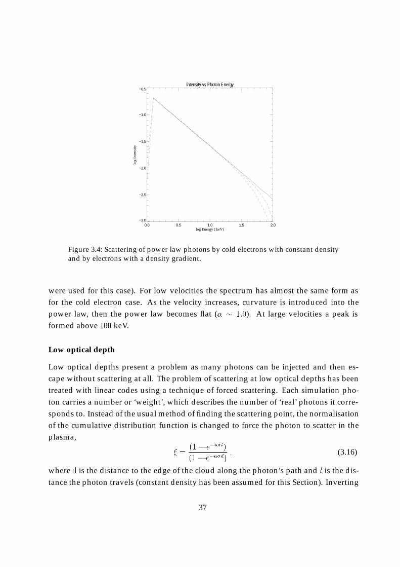
Intensity vs Photon Energy

0.0 0.5 1.0 1.5 2.0log Energy ( keV)

−3.0

−2.5

−2.0

−1.5

−1.0

−0.5

log

Inte

nsity

Figure 3.4: Scattering of power law photons by cold electrons with constant densityand by electrons with a density gradient.

were used for this case). For low velocities the spectrum has almost the same form asfor the cold electron case. As the velocity increases, curvature is introduced into thepower law, then the power law becomes flat (� � 1:0). At large velocities a peak isformed above 100 keV.

Low optical depth

Low optical depths present a problem as many photons can be injected and then es-cape without scattering at all. The problem of scattering at low optical depths has beentreated with linear codes using a technique of forced scattering. Each simulation pho-ton carries a number or ‘weight’, which describes the number of ‘real’ photons it corre-sponds to. Instead of the usual method of finding the scattering point, the normalisationof the cumulative distribution function is changed to force the photon to scatter in theplasma,

� =(1 � e�n�l)

(1� e�n�d); (3.16)

where d is the distance to the edge of the cloud along the photon’s path and l is the dis-tance the photon travels (constant density has been assumed for this Section). Inverting

37

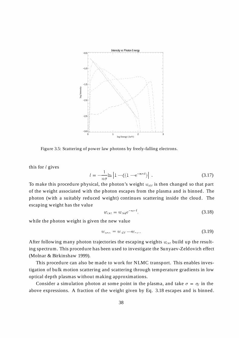
Intensity vs Photon Energy

0 1 2 3log Energy ( keV)

−3.0

−2.5

−2.0

−1.5

−1.0

−0.5

log

Inte

nsity

Figure 3.5: Scattering of power law photons by freely-falling electrons.

this for l gives

l = � 1

n�lnh1� �(1 � e�n�d)

i: (3.17)

To make this procedure physical, the photon’s weight wold is then changed so that partof the weight associated with the photon escapes from the plasma and is binned. Thephoton (with a suitably reduced weight) continues scattering inside the cloud. Theescaping weight has the value

wesc = wolde�n�d; (3.18)

while the photon weight is given the new value

wnew = wold � wesc: (3.19)

After following many photon trajectories the escaping weights wesc build up the result-ing spectrum. This procedure has been used to investigate the Sunyaev-Zeldovich effect(Molnar & Birkinshaw 1999).

This procedure can also be made to work for NLMC transport. This enables inves-tigation of bulk motion scattering and scattering through temperature gradients in lowoptical depth plasmas without making approximations.

Consider a simulation photon at some point in the plasma, and take � = �T in theabove expressions. A fraction of the weight given by Eq. 3.18 escapes and is binned.

38

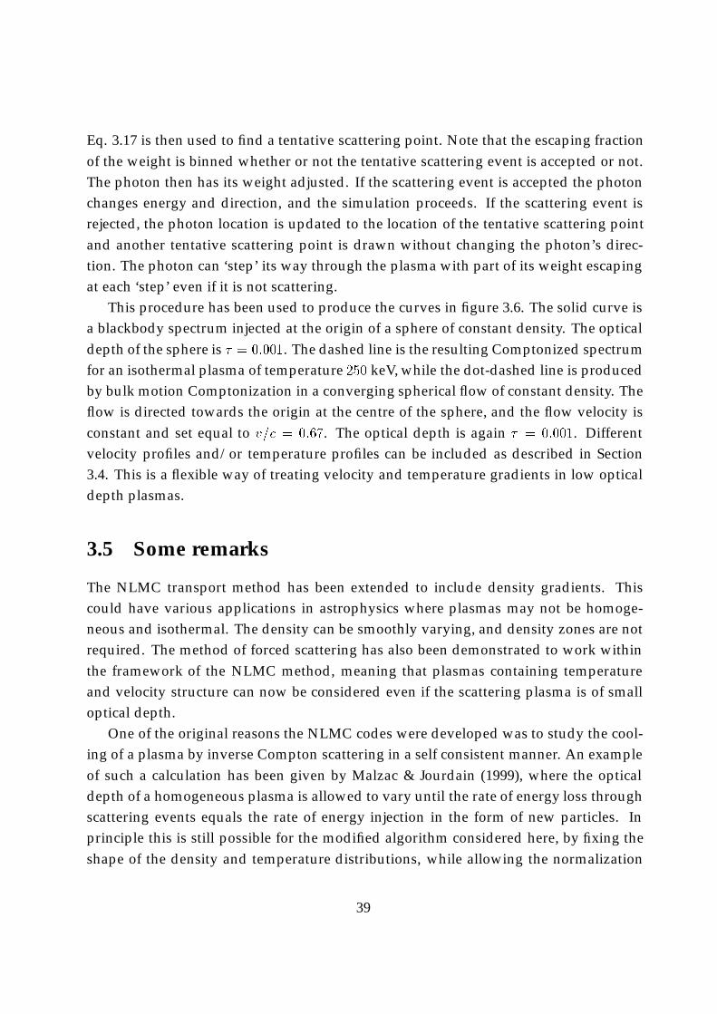
Eq. 3.17 is then used to find a tentative scattering point. Note that the escaping fractionof the weight is binned whether or not the tentative scattering event is accepted or not.The photon then has its weight adjusted. If the scattering event is accepted the photonchanges energy and direction, and the simulation proceeds. If the scattering event isrejected, the photon location is updated to the location of the tentative scattering pointand another tentative scattering point is drawn without changing the photon’s direc-tion. The photon can ‘step’ its way through the plasma with part of its weight escapingat each ‘step’ even if it is not scattering.

This procedure has been used to produce the curves in figure 3.6. The solid curve isa blackbody spectrum injected at the origin of a sphere of constant density. The opticaldepth of the sphere is � = 0:001. The dashed line is the resulting Comptonized spectrumfor an isothermal plasma of temperature 250 keV, while the dot-dashed line is producedby bulk motion Comptonization in a converging spherical flow of constant density. Theflow is directed towards the origin at the centre of the sphere, and the flow velocity isconstant and set equal to v=c = 0:67. The optical depth is again � = 0:001. Differentvelocity profiles and/or temperature profiles can be included as described in Section3.4. This is a flexible way of treating velocity and temperature gradients in low opticaldepth plasmas.

3.5 Some remarks

The NLMC transport method has been extended to include density gradients. Thiscould have various applications in astrophysics where plasmas may not be homoge-neous and isothermal. The density can be smoothly varying, and density zones are notrequired. The method of forced scattering has also been demonstrated to work withinthe framework of the NLMC method, meaning that plasmas containing temperatureand velocity structure can now be considered even if the scattering plasma is of smalloptical depth.

One of the original reasons the NLMC codes were developed was to study the cool-ing of a plasma by inverse Compton scattering in a self consistent manner. An exampleof such a calculation has been given by Malzac & Jourdain (1999), where the opticaldepth of a homogeneous plasma is allowed to vary until the rate of energy loss throughscattering events equals the rate of energy injection in the form of new particles. Inprinciple this is still possible for the modified algorithm considered here, by fixing theshape of the density and temperature distributions, while allowing the normalization

39

Intensity vs Photon Energy

−8 −6 −4 −2 0log Energy ( keV)

−15

−10

−5

0

log

Inte

nsity

Figure 3.6: Bulk motion scattering for � = 0:001, and thermal scattering for � =

0:001, for blackbody source photons.

of the density profile to move up and down. This corresponds to injecting more elec-trons or removing electrons, until the rate energy is removed equals the rate energy isbeing injected (which would be calculated by integrating over the density and temper-ature distributions). Such calculations are more demanding than pure Comptonizationproblems, and so have not been considered here.

A restriction on the method is that only photons are followed in the code, whichmeans that it cannot, for instance, study electron-positron pair cascades. In other re-spects it is a flexible way of treating the Comptonization problem.

40

References

Colpi, M. 1988, ApJ, 326, 223Gorecki, A. & Wilczewski, W. 1984, Acta Astron., 34, 141Hua, X. 1997, Com. Ph. 11, 660 (physics/9709023)L. D. Landau, L. D. & E. M. Lifshitz, E. M. 1971, ”The Classical Theory of Fields”, Chap-

ter 2, Section 12, (3rd edition, Pergamon Press)Malzac, J. & Jourdain, E. 1999, Pro. third INTEGRAL workshop, astro-ph/9901186Molnar, S. M. & Birkinshaw, M. 1999, ApJ, 523, 78 (astro-ph/9903444)Nelson, W. R. Hirayama, H. & Rogers, D. W. O. 1985, ”The EGS code system”, SLAC

Report 266, Stanford Linear Accelerator Center, section 2.4 (particle transport), seealso http://ehssun.lbl.gov/egs/egs.html

Pozdnyakov, L. A., Sobol, I. M. & Sunyaev, R. A. 1983, Ap.& Space Sci. Reviews, 2, 189Stern, B., et al. 1995, MNRAS, 272, 291Woodcock et al. 1965, ”Techniques used in the GEM code for Monte Carlo neutronics

calculations in reactors and other systems of complex geometry”, Proc. of the con-ference on the application of computing methods to reactor problems, ANL-7050,Argone National Lab.

41

Part III

Astrophysical

42

Chapter 4

Comptonized Spectra from AGN

The standard two-phase disk–corona model for the high-energy spectra of active galac-tic nuclei (AGN) is modified to include an additional component — an outflow or windwhich is assumed to provide an additional source of disk cooling. Earlier slab disk–corona models predict a spectral index which is consistent with observations only ifall the accretion power is dissipated in the corona. For the models investigated here,energy spectral indices that are consistent with observations can be obtained with lessaccretion power being dissipated in the corona, as a result of an outflow/wind. How-ever, the luminosity ratio of the hard component to the soft component is required to begreater than one, which is not consistent with observations.

4.1 Accretion disk coronae

The accretion disks that exist in AGN (and also in X-ray binaries) are often modeledusing the standard geometrically thin, optically thick formalism of Shakura & Sunyaev(1973). Such a description, however, cannot account for the observed emission at highenergies; the inflowing material cannot radiate at energies higher than the local black-

body temperature, Tbb =�

L4�r2�

�1=4 ' 2 � 105 (L=LEdd)1=4(r=10rg)

�1=2(M=107M�)�1=4K.

Two possible explanations for the observed high energy emission are: a hot accretiondisk solution, first suggested by Shapiro et al. (1976), and an accretion disk corona, firstproposed by Liang & Price (1977) and Bisnovatyi-Kogan & Blinnikov (1977). The hotdisk solution has been found to be thermally unstable, however.

The accretion disk corona is an optically thin layer of plasma above and below theinnermost regions of the accretion disk, where the bulk of the accretion power is ulti-

43

mately dissipated. Although the heating mechanism for accretion disk coronae is notyet known, the current consensus is that magnetic processes are involved (see e.g. Miller& Stone 2000). The primary cooling mechanism is inverse Compton scattering off softphotons emitted by the disk.

The observed spectral energy distributions of most AGN (Seyfert galaxies and radio-quiet quasars) reveal a power law at X-ray energies with a spectral index that variesremarkably little from a value close to unity. Observed spectral indices of Seyferts fallin the range � � 0:80�1:10 (Pounds et al. 1990, Nandra & Pounds 1994). This has led tothe formulation of the standard two-phase disk–corona models, proposed by Haardt &Maraschi (1991, 1993) (see also Svensson & Zdziarski 1994, Haardt et al. 1994, 1997) andsubsequent various modifications (e.g. Dove, Wilms & Begelman 1997 and referencestherein). These models can reproduce the observed X-ray spectra with spectral indices� ' 1, consistent with the values deduced from observations. The other main observa-tional result is that the ratio of the luminosity in the hard component to the luminosityin the soft component LC=Ls is typically found to be less than one.

The key ingredients of the disk–corona models are a ‘standard’ optically thick (i.e.‘cool’), geometrically thin accretion disk surrounded by an optically thin (i.e. ‘hot’), ex-tended atmosphere/corona. This two-phase system interacts via a radiation field that islargely generated by thermal reprocessing effects; the X–rays and –rays are producedin the diffuse corona as a result of upscattering (Comptonization) of soft (optical/UV)disk photons, which are in turn produced partly by the re–emission of photoabsorbedX–rays and partly by radiating away energy directly dissipated in the disk. For a slabcoronal geometry it is required that the fraction, f , of the accretion power dissipatedin the corona be close to unity, so as to obtain a spectral index � � 1. (e.g. Haardt,Maraschi & Ghisellini 1994). However, in its simplest form the slab corona geometrycannot account for the spectral index of all Seyferts (Petrucci et al. 2000), because thespectral index obtained cannot be made to be less than one, as is sometimes observed.

To resolve these difficulties, Haardt et al. (1994) introduced a covering factor so thatsome fraction of the soft photons escape from the disk without passing through thecorona and being Comptonized. The parameter f can then take a smaller value becausesuch a ‘photon starved’ corona cools less efficiently, so less accretion power is requiredfor a given coronal temperature. Because such a corona is in general hotter, the ampli-fication factor is larger, and spectral indices that are less than unity can be produced.Other proposed resolutions to this problem so far include the introduction of bulk mo-tion of coronal material away from the disk (Beloborodov 1999) and the possibility of ahighly ionised disk surface (Nayakshin, Kazanas & Kallman 2000).

44

What these models have in common is the idea of reducing the flux of reprocesseddisk photons entering the corona. Because the corona cools via inverse Compton scat-tering of these photons, the cooling rate is reduced and the hotter corona produces aharder spectra. For instance, a covering factor enables reprocessed soft disk photons toescape without entering the corona. Photons that scatter in the bulk motion model arepreferentially scattered away from the disk (if the bulk flow is directed away from thedisk), reducing the number of photons that are reprocessed by the disk. The ioniseddisk model also reduces reprocessing by the disk as many photons are reflected awaydue to the larger albedo.

One component that has been generally overlooked in disk–corona models to dateis a disk outflow. Despite the understanding that outflows may be common in thesesystems (for a discussion see e.g. Heyvaerts 1992), the effect of outflows on the energybalance of the system and hence their effect on the high–energy spectra are only nowbeing investigated.

If a disk wind exists in Seyfert galaxies, it will extract energy from the accretiondisk, reducing the number of soft photons that are required to dissipate the accretionpower in the disk. As the disk emits fewer soft photons, coronal electrons cannot cool asefficiently by inverse Compton scattering, and so the corresponding coronae are hotter,leading to harder spectra.

The exact mechanism producing winds from accretion disks has not been defini-tively established, but one possibility is that the outflow is an electromagnetic/Poynting-flux dominated wind (Michel 1987). Such an outflow could be launched from a mag-netised accretion disk, and the fraction of available accretion power extracted from thedisk can be of order one (Lovelace, Wang & Sulkanen 1987).

Other possibilities are that a centrifugally driven wind can remove a significantamount of disk energy (Blandford & Payne 1982), or, if the accretion rate is low, a mod-ification to the advection dominated accretion flow (ADAF) model has been proposedthat includes a powerful wind that carries away mass and energy from the accretingmaterial (Blandford & Begelman 1999). Compton heated winds are probably ruled out,however, as the Compton temperature is much less than the virial temperature (Begel-man, McKee & Shields 1983).

Here, a disk–corona model is considered in which the disk and the corona are cou-pled in the usual manner, but where some of the energy in the disk, including some ofthe energy the disk has absorbed from hard illuminating photons, is dissipated in anoutflow or wind. This provides an additional avenue for disk cooling (figure 4.1).

This model is then compared to a second possible disk–corona model involving out-

45

flows and magnetic fields (de Kool, Bicknell & Kuncic 1999). This model considers anoutflowing corona in which the corona is heated predominantly by the dissipation ofbuoyant magnetic flux tubes emerging from the disk.

The spectral indices predicted by these ‘windy’ disk–corona models are determinedand compared to those predicted by the standard two-phase model.

4.2 A modified two-phase model

The model developed here follows the method of Haardt & Maraschi (1991), whichdraws on energy balance equations for the disk and corona to parametrise the partition-ing of accretion power Pa between the phases.

4.2.1 Energy Balance

Initially, some fraction f of the total accretion power is dissipated in the corona, whilethe remaining fraction (1 � f)Pa is dissipated directly in the disk. Because the coronalgeometry in particular is still uncertain, it is taken to be a simple slab coronal geometry.Geometrical factors would further complicate the analysis without providing additionalinsight.

The total luminosity emitted by the corona is given by ALs where A is the amplifi-cation factor due to Comptonization of the soft input photon luminosity Ls. Thus, theCompton luminosity is LC = LuC + LdC = (A � 1)Ls where LuC and LdC are upward-directed and downward-directed components ofLC, respectively. The downward-directedphotons can produce a reflected component in the X–ray spectrum, Lref = aLdC, wherea is the albedo, and the remaining fraction is absorbed by the disk.

Not all of the absorbed radiation need be re–emitted at soft energies and contributeto Ls, if some fraction of this energy is removed via a disk wind. Because of the un-certainty in the exact physics responsible for launching disk winds, in this work theefficiency of the wind is parameterised by �, where � is the ratio of the energy extractedfrom the disk by the wind to the luminosity of the hard photons absorbed by the disk.This means that a fraction of the absorbed power (1 � �)(1 � a)LdC contributes to Ls.Other parameterisations are certainly possible, but are essentially equivalent mathemat-ically.

With this choice of parameterisation, the rate of energy deposited in the wind from

46

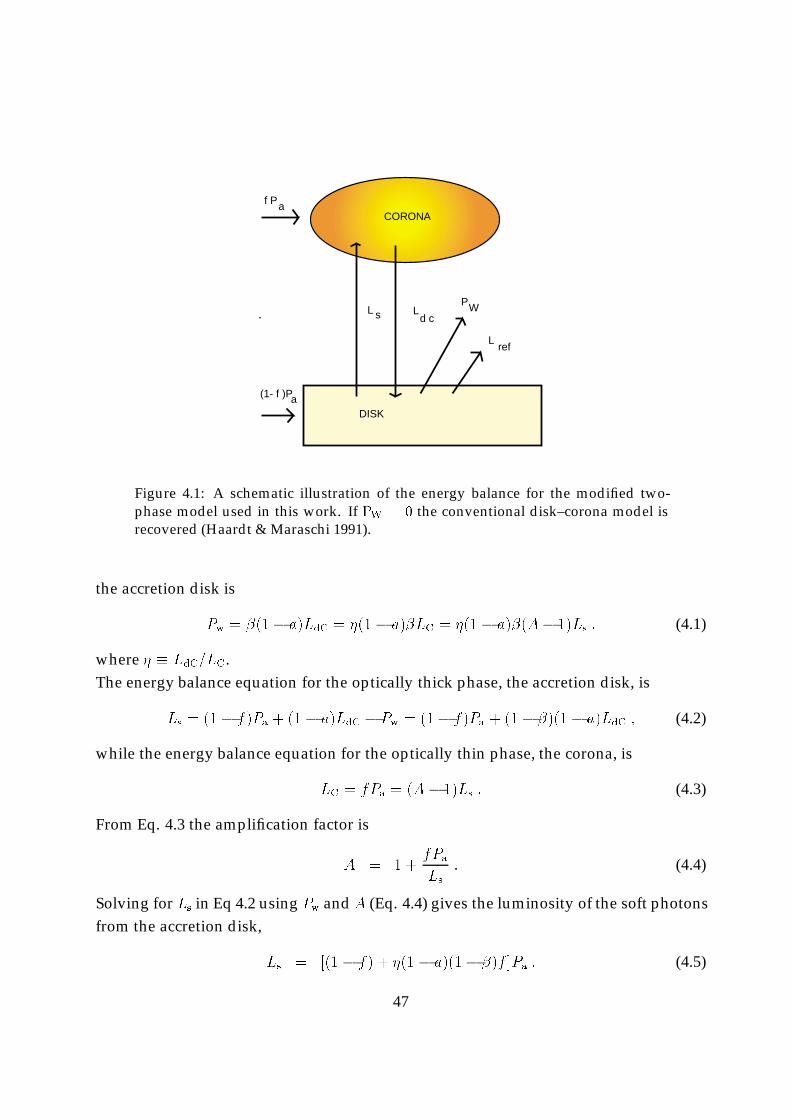
DISK

CORONA

L

L

(1- f )P

L

f P

PWs d c

ref

a

a

Figure 4.1: A schematic illustration of the energy balance for the modified two-phase model used in this work. If PW = 0 the conventional disk–corona model isrecovered (Haardt & Maraschi 1991).

the accretion disk is

Pw = �(1� a)LdC = �(1� a)�LC = �(1� a)�(A� 1)Ls : (4.1)

where � � LdC=LC.The energy balance equation for the optically thick phase, the accretion disk, is

Ls = (1� f)Pa + (1� a)LdC � Pw = (1� f)Pa + (1� �)(1� a)LdC ; (4.2)

while the energy balance equation for the optically thin phase, the corona, is

LC = fPa = (A� 1)Ls : (4.3)

From Eq. 4.3 the amplification factor is

A = 1 +fPa

Ls: (4.4)

Solving for Ls in Eq 4.2 using Pw and A (Eq. 4.4) gives the luminosity of the soft photonsfrom the accretion disk,

Ls = [(1� f) + �(1 � a)(1� �)f ]Pa : (4.5)

47

Solving for A using Eq. 4.4 and Eq. 4.5 yields the desired amplification factor

A = 1 +f

1� f [1 � �(1 � a)(1� �)]; (4.6)

which is independent of the total accretion power Pa. Note that if � is set to zero (theno wind case), the original amplification factor given in Haardt & Maraschi (1991) isrecovered.

The values of � considered in this Chapter run from zero to one. Note that � = 1:0

does not correspond to all of the disk energy being removed in the wind, only somefraction (Eq. 4.1) there of. A larger value for � is allowed, which would have the effectof reducing the amplification factor (Eq. 4.6).

The total outward luminosity is

Lout = Ls + LuC + Lref ; (4.7)

whereLuC = (1 � �)fPa ; (4.8)

is the luminosity of the upward-directed photons.It should also be noted that the accretion power in the system is carried out not only

by the upward-directed Comptonized photons from the hot corona but also by the windfrom the accretion disk. Using Eq. 4.1 & Eq. 4.4 gives PW = �(1 � a)�f � 0:51 since� and f can at most be equal to unity, so that up to half of the accretion power can becarried away by the wind rather than the radiation. This is why Lout does not equal Pa(cf. Haardt & Maraschi 1991), as some power is dissipated in the wind from the disk. Itis, however, not difficult to verify Lout + Pw = Pa.

4.3 Spectral Index and Temperature

To determine the observational effects of a wind, it is necessary to determine the spec-trum of this model. To do this, an iterative approach is used to solve for the parametersof the corona.

4.3.1 Iterative Method

For optical depth (� � n�Th with n the electron density, �T the Thompson cross-sectionand h the height of the slab corona above the disk) less than one, the Comptonized

48

spectrum can be approximated by a power law

I(�) = I(�0)��

�0

���; (4.9)

where� = � ln (� )

ln (A1); (4.10)

(Rybicki & Lightman 1979, Pozdnyakov, Sobol & Sunyaev 1983), �0 is the average energyof the soft photons, and A1 is the amplification factor describing the average energy gainfor a single scattering. In Titarchuk & Lyubarskij (1995) more accurate expressions for�, which take into account the effects due to geometry and optical depths, are given (seealso Haardt & Maraschi 1993). However, for the purpose of this study, using the simpleexpression for � in Eq. 4.10 or the accurate expressions given elsewhere will not lead toqualitatively very different results. In terms of the corona temperature (in units of theelectron rest mass energy � = kTc=mec

2),

A1 = 16�2 + 4� + 1 ; (4.11)

(e.g. Haardt, Maraschi & Ghisellini 1997). Assuming that Ls ' I(�0)�0, the energy gainedby the photons traversing the corona is then given by

A� 1 =1

I(�0)�0

Z 3kTc

�1I(�) d� (4.12)

= (1� �)�124 3kTc

�0

!1��

�A11��

35 ; (4.13)

where �1 = �0A1 is the energy gain due to the first scattering of the soft photons in thecorona, �0 is the average energy of the soft input photons and � is the spectral index ofthe resulting Comptonized spectrum.

The expression for the amplification factor A, in Eq. 4.6, is substituted into Eq. 4.13and the resulting expression solved iteratively for the spectral index � as a function of� and � for various values of f and �.

The effects of the spectral temperature of the soft black body photons on the spectralindex in the energy range 2-10 keV is generally insignificant due to the large energy shiftper scattering event. Therefore the mean photon energy is fixed to �0 = 50 eV in thisstudy. For simplicity, it is assumed that the scattering albedo and the downscatteringparameter have constant values of a = 0.15 and � = 0.6 respectively. (A detail discussionon the effects due to anisotropy (� 6= 0:5) and the variations in a and � with the optical

49

depth can be found in Haardt & Maraschi 1993). For the � = 0 case (i.e. the conventionaltwo-phase no wind disk–corona model) the ‘��Log(� )’ and ‘Log(�)�Log(� )’ relationsare consistent with those in Figure 1 of Haardt & Maraschi (1991). (The exact valuesof a and � considered by those authors were 0:15 and 0:6 respectively, however theirexpression of A1 was obtained by a fit to Monte Carlo simulations. Their results can bereproduced here if a = 0.17 and � = 0.5.)

Now consider spectra produced using the amplification factor given in Eq. 4.6 withf = 0.5 and for various values of �. The spectral index � and the logarithm of thecoronal temperature � as functions of the optical depth � are shown in Figures 4.2a andb. Figure 4.3a, and b shows the results for the cases with � = 0:75 and various valuesof f . Figure 4.4a, and b shows the results for the extreme cases of f = 1.0, � = 0.99,and f = 0.9999, � = 1.0. For comparison, we also show the ‘� � Log(� )’ relation of theconventional two-phase disk–corona model with f = 1 as the solid line in Figure 4.4a.

The inclusion of a disk wind term in this modified disk–corona model removes en-ergy from the disk that would otherwise have gone into soft photon emission. Theaccretion disk emits fewer soft photons, and so the corresponding corona is hotter andphotons can be up-scattered to higher energies. While the Haardt & Maraschi (1991)amplification factor can never be larger than about 3.4, the amplification factors in thewind model considered here can in principle be arbitrarily large, resulting in much flat-ter spectra.

To investigate the dependence of the spectra on the wind parameter in a more de-tailed way, figure 4.5 presents the results of Monte Carlo simulations of Comptonizationin a plane-parallel slab geometry with an isotropic point source of blackbody photonslocated on the disk midplane. The temperature of the blackbody source was set equal tothat of the monoenergetic photon source used in all the semi-analytic calculations. Thetemperature of the coronal electrons was determined by the energy balance as describedabove.

For all curves, the optical depth is � = 0:1. The solid curve is the spectrum producedwhen the electron temperature is given by the Haardt & Maraschi amplification factor(1991), which gives a temperature of � = 0:45 (f = 1:0 case). The other curves are thespectra produced when the electron temperature is given by the amplification factorpresented in Section 4.2.1. For the dashed, the dot-dashed and the dot-dot-dot-dashedcurves, the temperature � is 0.54, 0.68, 0.80. This corresponds to f = 1:0 and � =

0:5; 0:8; 0:9. The peak just above 100 eV is the blackbody injection spectrum.As the wind parameter � is increased, the spectra become progressively flatter. The

temperature of the electrons increases by about 200 keV between the � = 0:5 case and

50

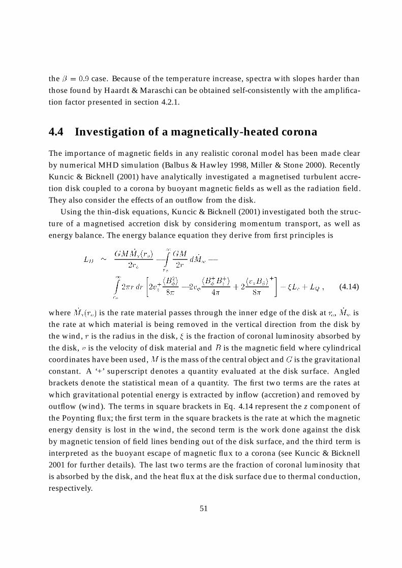
the � = 0:9 case. Because of the temperature increase, spectra with slopes harder thanthose found by Haardt & Maraschi can be obtained self-consistently with the amplifica-tion factor presented in section 4.2.1.

4.4 Investigation of a magnetically-heated corona

The importance of magnetic fields in any realistic coronal model has been made clearby numerical MHD simulation (Balbus & Hawley 1998, Miller & Stone 2000). RecentlyKuncic & Bicknell (2001) have analytically investigated a magnetised turbulent accre-tion disk coupled to a corona by buoyant magnetic fields as well as the radiation field.They also consider the effects of an outflow from the disk.

Using the thin-disk equations, Kuncic & Bicknell (2001) investigated both the struc-ture of a magnetised accretion disk by considering momentum transport, as well asenergy balance. The energy balance equation they derive from first principles is

LD ' GM _Ma(ro)

2ro�

1Zro

GM

2rd _Mw �

1Zro

2�r dr

"2v+z

hB2�i

8�� 2v�

hB+�B

+z i

4�+ 2

hvzB�i8�

+#+ �Lc + LQ ; (4.14)

where _Ma(ro) is the rate material passes through the inner edge of the disk at ro, _Mw isthe rate at which material is being removed in the vertical direction from the disk bythe wind, r is the radius in the disk, � is the fraction of coronal luminosity absorbed bythe disk, v is the velocity of disk material and B is the magnetic field where cylindricalcoordinates have been used, M is the mass of the central object and G is the gravitationalconstant. A ‘+’ superscript denotes a quantity evaluated at the disk surface. Angledbrackets denote the statistical mean of a quantity. The first two terms are the rates atwhich gravitational potential energy is extracted by inflow (accretion) and removed byoutflow (wind). The terms in square brackets in Eq. 4.14 represent the z component ofthe Poynting flux; the first term in the square brackets is the rate at which the magneticenergy density is lost in the wind, the second term is the work done against the diskby magnetic tension of field lines bending out of the disk surface, and the third term isinterpreted as the buoyant escape of magnetic flux to a corona (see Kuncic & Bicknell2001 for further details). The last two terms are the fraction of coronal luminosity thatis absorbed by the disk, and the heat flux at the disk surface due to thermal conduction,respectively.

51

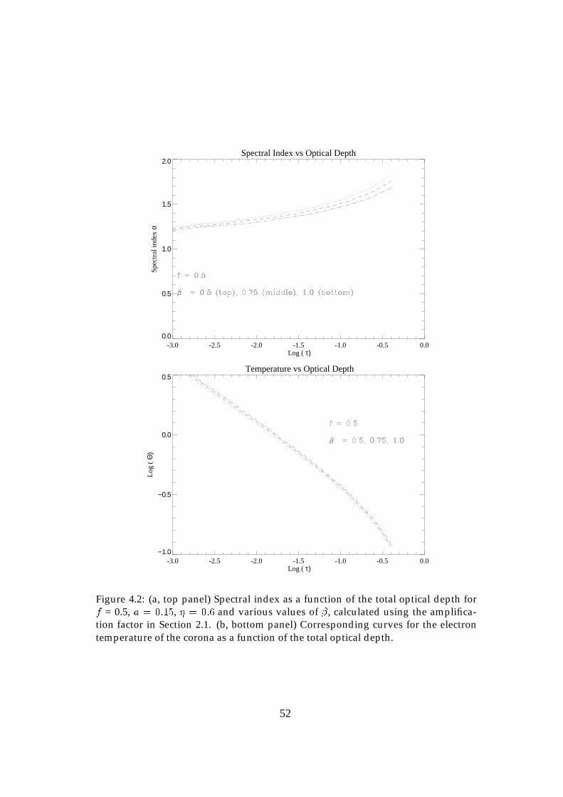
Spectral Index vs Optical Depth

-3.0 -2.5 -2.0 -1.5 -1.0 -0.5 0.0 Log ( τ)

0.0

0.5

1.0

1.5

2.0Sp

ectr

al in

dex

α

Temperature vs Optical Depth

-3.0 -2.5 -2.0 -1.5 -1.0 -0.5 0.0 Log ( τ)

−1.0

−0.5

0.0

0.5

Log

( Θ

)

Figure 4.2: (a, top panel) Spectral index as a function of the total optical depth forf = 0.5, a = 0:15, � = 0:6 and various values of �, calculated using the amplifica-tion factor in Section 2.1. (b, bottom panel) Corresponding curves for the electrontemperature of the corona as a function of the total optical depth.

52

Spectral Index vs Optical Depth

-3.0 -2.5 -2.0 -1.5 -1.0 -0.5 0.0 Log ( τ)

0.0

0.5

1.0

1.5

2.0Sp

ectr

al in

dex

α

Temperature vs Optical Depth

-3.0 -2.5 -2.0 -1.5 -1.0 -0.5 0.0 Log ( τ)

−1.0

−0.5

0.0

0.5

1.0

Log

( Θ

)

Figure 4.3: (a, top panel) Spectral index as a function of the total optical depth for� = 0:75, a = 0:15, � = 0:6 and various values of f . (b, bottom panel) Correspondingcurves for the electron temperature of the corona as a function of the total opticaldepth .

53

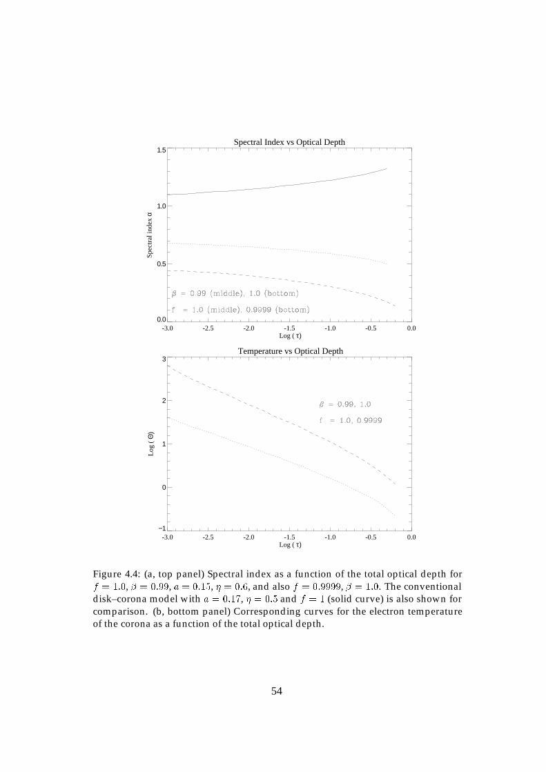
Spectral Index vs Optical Depth

-3.0 -2.5 -2.0 -1.5 -1.0 -0.5 0.0 Log ( τ)

0.0

0.5

1.0

1.5Sp

ectr

al in

dex

α

Temperature vs Optical Depth

-3.0 -2.5 -2.0 -1.5 -1.0 -0.5 0.0 Log ( τ)

−1

0

1

2

3

Log

( Θ

)

Figure 4.4: (a, top panel) Spectral index as a function of the total optical depth forf = 1:0, � = 0:99, a = 0:15, � = 0:6, and also f = 0:9999, � = 1:0. The conventionaldisk–corona model with a = 0:17, � = 0:5 and f = 1 (solid curve) is also shown forcomparison. (b, bottom panel) Corresponding curves for the electron temperatureof the corona as a function of the total optical depth.

54

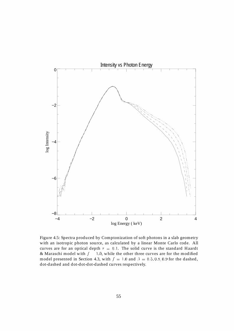
Intensity vs Photon Energy

−4 −2 0 2 4log Energy ( keV)

−8

−6

−4

−2

0

log

Inte

nsity

Figure 4.5: Spectra produced by Comptonization of soft photons in a slab geometrywith an isotropic photon source, as calculated by a linear Monte Carlo code. Allcurves are for an optical depth � = 0:1. The solid curve is the standard Haardt& Maraschi model with f = 1:0, while the other three curves are for the modifiedmodel presented in Section 4.3, with f = 1:0 and � = 0:5; 0:8; 0:9 for the dashed,dot-dashed and dot-dot-dot-dashed curves respectively.

55

Parametrising the magnetic and conduction terms as fBPG and qcfBPG respectively,the following expression for the amplification factor is obtained;

A� 1 =Lc

LD=

(1� qc)fB1� fw � fB[1� �(1 � qc)� qc]

; (4.15)

where fw, fB, and qc represent the fraction of energy in the disk outflow, the magneticheating of the corona, and the thermal conductivity of the disk, respectively, and � is thefraction of coronal luminosity absorbed by the disk. Following the same procedure asfor the previous Section, this amplification factor is used to find the spectral index andcoronal temperature as a function of optical depth.

Although de Kool et al. derive expressions for the parameter fB , they do not ex-plicitly suggest values for the other parameters. Here, to explore the parameter spaceof the amplification factor given by Eq. 4.15, the value of a given parameter is variedwhile other parameters are held constant. In figure 4.6a, the fraction of accretion powerreleased into a wind is varied. The value of the spectral index drops to unity as fw in-creases. Figure 4.6 b shows the corresponding temperature of the corona for the samevalues. Figure 4.7a, and b, show the results for the cases with fw = 0.5, qc = 0:1 andvarious values of fB. Figure 4.8a, and b, show the results for the cases with fw = 0.5,fB = 0:5 and various values of qc.

One sees the same qualitative behaviour as for the previously considered amplifica-tion factor, given in Eq. 4.6, in that a hotter corona produces a flatter spectrum. Againthe amplification factor can be larger than the Haardt & Maraschi value.

The parameters fw and fB appear to be the most important factors in producinga hotter corona, while varying the coronal thermal conductivity has a relatively smalleffect on the spectral index.

Note here that one can write the wind parameter of Section 4.2.1 in terms of the deKool et al. wind parameter fw using Eq. 4.3 and Eq. 4.4

� =1

(1� a)�f

Pw

PG=

1

(1 � a)�ffw (4.16)

where PwPG

is taken to be the same as fw . This relation, when substituted into Eq. 4.6 givesthe de Kool et al amplification factor if � = (1 � a)� and qc = 0. Thus over some of theparameter space the two models considered here are equivalent.

56

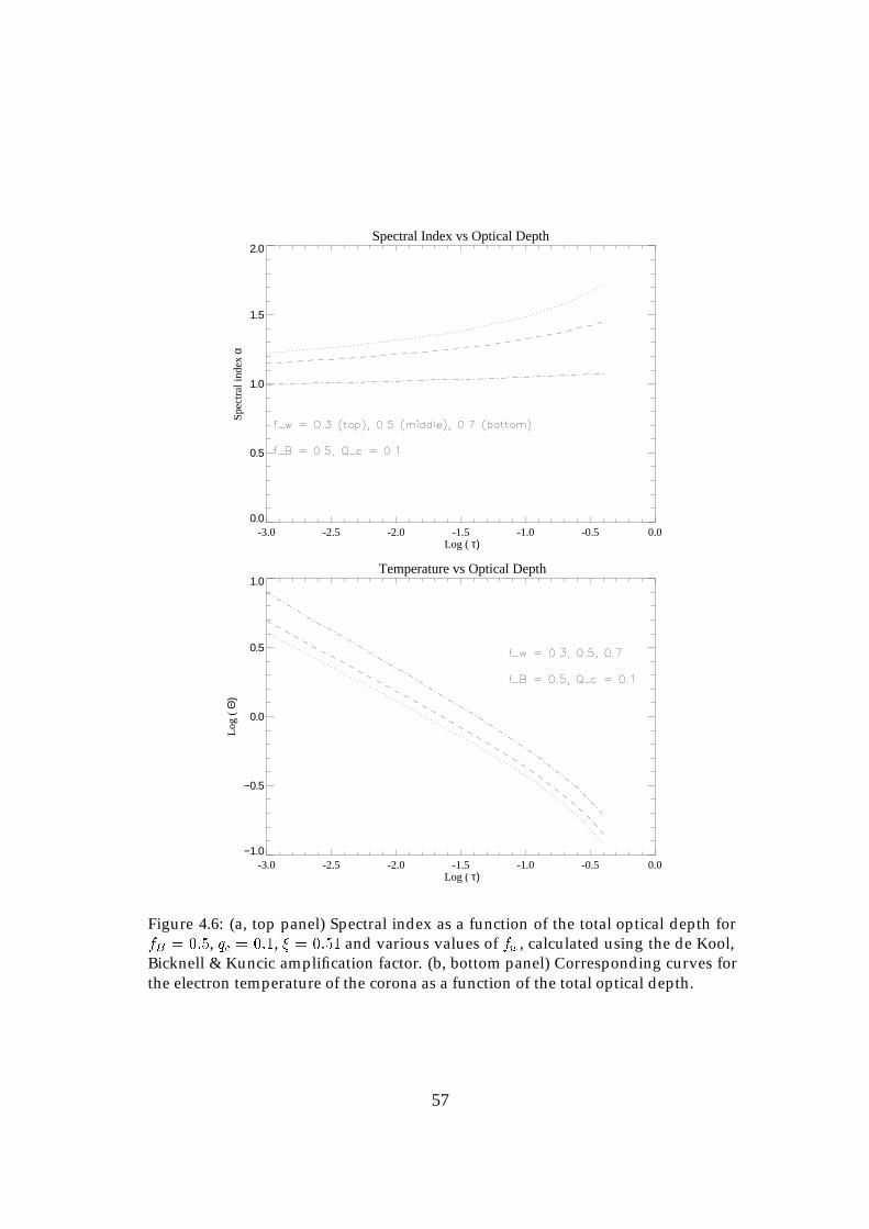
Spectral Index vs Optical Depth

-3.0 -2.5 -2.0 -1.5 -1.0 -0.5 0.0 Log ( τ)

0.0

0.5

1.0

1.5

2.0Sp

ectr

al in

dex

α

Temperature vs Optical Depth

-3.0 -2.5 -2.0 -1.5 -1.0 -0.5 0.0 Log ( τ)

−1.0

−0.5

0.0

0.5

1.0

Log

( Θ

)

Figure 4.6: (a, top panel) Spectral index as a function of the total optical depth forfB = 0:5, qc = 0:1, � = 0:51 and various values of fw , calculated using the de Kool,Bicknell & Kuncic amplification factor. (b, bottom panel) Corresponding curves forthe electron temperature of the corona as a function of the total optical depth.

57

Spectral Index vs Optical Depth

-3.0 -2.5 -2.0 -1.5 -1.0 -0.5 0.0 Log ( τ)

0.0

0.5

1.0

1.5

2.0Sp

ectr

al in

dex

α

Temperature vs Optical Depth

-3.0 -2.5 -2.0 -1.5 -1.0 -0.5 0.0 Log ( τ)

−1.0

−0.5

0.0

0.5

1.0

Log

( Θ

)

Figure 4.7: (a, top panel) Spectral index as a function of the total optical depth forfw = 0:5, qc = 0:1, � = 0:51 and various values of fB. (b, bottom panel) Corre-sponding curves for the electron temperature of the corona as a function of the totaloptical depth .

58

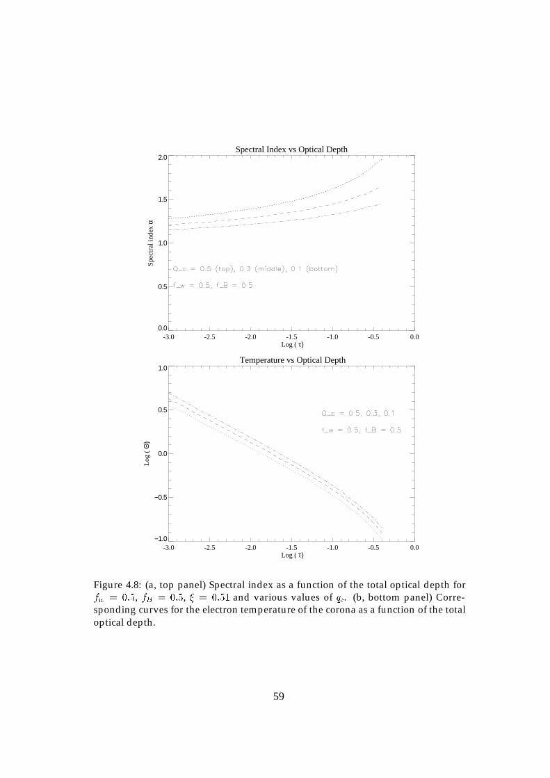
Spectral Index vs Optical Depth

-3.0 -2.5 -2.0 -1.5 -1.0 -0.5 0.0 Log ( τ)

0.0

0.5

1.0

1.5

2.0Sp

ectr

al in

dex

α

Temperature vs Optical Depth

-3.0 -2.5 -2.0 -1.5 -1.0 -0.5 0.0 Log ( τ)

−1.0

−0.5

0.0

0.5

1.0

Log

( Θ

)

Figure 4.8: (a, top panel) Spectral index as a function of the total optical depth forfw = 0:5, fB = 0:5, � = 0:51 and various values of qc. (b, bottom panel) Corre-sponding curves for the electron temperature of the corona as a function of the totaloptical depth.

59

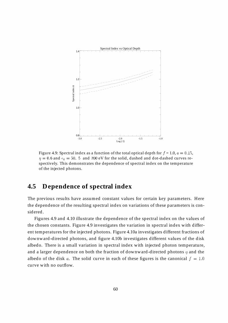
Spectral Index vs Optical Depth

-3.0 -2.5 -2.0 -1.5 -1.0 Log ( τ)

0.8

1.0

1.2

1.4

Spec

tral

inde

x α

Figure 4.9: Spectral index as a function of the total optical depth for f = 1.0, a = 0:15,� = 0:6 and �0 = 50; 5 and 200 eV for the solid, dashed and dot-dashed curves re-spectively. This demonstrates the dependence of spectral index on the temperatureof the injected photons.

4.5 Dependence of spectral index

The previous results have assumed constant values for certain key parameters. Herethe dependence of the resulting spectral index on variations of these parameters is con-sidered.

Figures 4.9 and 4.10 illustrate the dependence of the spectral index on the values ofthe chosen constants. Figure 4.9 investigates the variation in spectral index with differ-ent temperatures for the injected photons. Figure 4.10a investigates different fractions ofdownward-directed photons, and figure 4.10b investigates different values of the diskalbedo. There is a small variation in spectral index with injected photon temperature,and a larger dependence on both the fraction of downward-directed photons � and thealbedo of the disk a. The solid curve in each of these figures is the canonical f = 1:0

curve with no outflow.

60

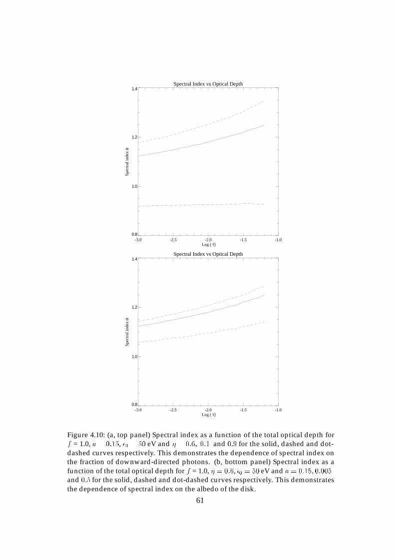
Spectral Index vs Optical Depth

-3.0 -2.5 -2.0 -1.5 -1.0 Log ( τ)

0.8

1.0

1.2

1.4

Spec

tral

inde

x α

Spectral Index vs Optical Depth

-3.0 -2.5 -2.0 -1.5 -1.0 Log ( τ)

0.8

1.0

1.2

1.4

Spec

tral

inde

x α

Figure 4.10: (a, top panel) Spectral index as a function of the total optical depth forf = 1.0, a = 0:15, �0 = 50 eV and � = 0:6; 0:1 and 0:9 for the solid, dashed and dot-dashed curves respectively. This demonstrates the dependence of spectral index onthe fraction of downward-directed photons. (b, bottom panel) Spectral index as afunction of the total optical depth for f = 1.0, � = 0:6, �0 = 50 eV and a = 0:15; 0:005and 0:5 for the solid, dashed and dot-dashed curves respectively. This demonstratesthe dependence of spectral index on the albedo of the disk.

61

4.6 Conclusion

As mentioned in the introduction, a disk wind extracts energy from the accretion disk,leading to a larger coronal amplification factor and harder spectra. The ‘windy’ disk–corona then mimics a photon starved geometry. This can be seen, for example, in fig-ures 4.4a and b. The spectral index curves are well below 1, and the corresponding coro-nal temperatures are larger. This behaviour is expected for ‘patchy’ coronae. Therefore,the inclusion of an outflow has approximately the same effect as a covering factor, inthat energy can now leave the system (in the form of a wind, rather than soft photons).

As mentioned in Section 4.1, observed spectral indices of Seyferts fall in the range� � 0:80 � 1:10. The original two-phase model accounts for spectral indices of one andabove, but cannot account for � < 1. In particular, by the inclusion of a disk wind, thesemodified models can in principle account for AGN with spectral indices smaller thanone.

It is possible to relax the f = 1 requirement for a slab corona to a certain extent, if thewind parameter is large. Considering the first modified disk–corona model, a spectralindex curve similar to the ‘�� Log(� )’ relation for f = 1 given in Haardt & Maraschi(1991) can be reproduced by the model with the parameters f = 0:75 and � = 0:75. Aspectral index much less than unity can also be obtained, if appropriate values for theparameters are chosen (figure 4.4a).

As noted previously, the two models considered here are equivalent over some ofthe parameter space if qc = 0. Using the second model (de Kool et al. 1999) a spectralindex at or less than unity can also be obtained, again if the corona is wind dominated,for the same reason as discussed above. For example, in figure 4.7a, ‘�’ is close to unityfor fB = 0.5 if ‘fw’ is 0.7. This model can therefore also account for Seyfert galaxies thathave Comptonized components with � � 1.

The shape of the Comptonized spectrum depends on both temperature and opti-cal depth. The spectral index curves for the standard disk–corona model increase withincreasing ‘� ’, while the coronal temperature is decreasing. That is, the trend of the spec-tral index is determined predominantly by optical depth. For the first model consideredhere, if the wind parameter and the heating rate are both large, the spectral index canbe made to decrease with increasing ‘� ’ and follow the temperature in trending down-ward. The spectral index is now in a regime where it is being determined mainly by thetemperature (figure 4.4a).

Compared to the Haardt & Maraschi model, the corona for both models can be sub-stantially hotter. The observational constraints on the temperature of the coronal plasma

62

depend on the energy of the spectral cut-off, which is not well determined. However,the maximum temperature seem to be in the range of a few hundreds of keV. This wouldrestrict these models to an optical depth of � 0:1 or greater as at lower optical depthselectron cooling is inefficient.

It should be mentioned that to determine if the higher coronal temperatures requiredby ‘windy’ disk–coronae are reasonable requires a non-linear Monte Carlo simulationof the type performed by Stern et al. (1995). Such a simulation allows the coronalheating to balance inverse Compton cooling and determine a coronal temperature self-consistently (whereas linear Monte Carlo simulations assume a temperature as input).

An electromagnetic wind is almost impossible to directly observe (Michel 1987). Ifthe wind is of the type associated with an ADAF or an inflow/outflow solution, ob-servation of the wind is still difficult, although the wind could potentially be observedif the wind passes through a terminal shock (Blandford & Begelman, 1999). In thiscase, it is difficult to know what, if any, observational relationship might exist betweenshocked-wind emission and the power law index.

One possible observational effect is whether there is a correlation between the vari-ability of the soft component and the variability of the hard component. If the windis unstable, and some material is entrained with the wind, and the system is being ob-served along a line of sight that passes through the wind, then the line-of-sight electrondensity will be time-dependent. The amount of absorption soft photons experience willvary, while the hard photons will experience little absorption. Therefore, the soft com-ponent will be fluctuating with respect to the hard component.

The drawbacks of the models are that producing the observed value of the hard tosoft components is not possible, as the amplification factor required for a flat spectrumgives an LC=Ls ratio of greater than one. Observationally, the ratio LC=Ls is typicallyless than one. This has also been a problem with previous slab corona models. Also,as this work considers the albedo of the disk to be constant, the models cannot accountfor the observed correlation between spectral index and the amount of disk reflection.This correlation seems to require complex ionisation structure, as investigated by Done& Nayakshin (2001), or perhaps bulk motion in the corona (Beloborodov 1999).

In summary, the spectra from disk–corona models with outflows have been investi-gated. There exists a regime in which the dependence of spectral index on temperatureis the opposite of that usually expected; cooler coronae may produce harder spectra(figure 4.4a). Because of the formal similarity between these windy models and photon-starved models, one might speculate that this result may also hold for very photon-starved models. With both of the models considered in this work, spectral indices con-

63

sistent with observations can be obtained in a slab geometry without requiring all theaccretion power to be dissipated directly to the corona, because an outflow has approx-imately the same effect on the system as a covering factor.

64

References

Balbus, S. A. & Hawley, J. F. 1998, “Accretion processes in astrophysical systems; somelike it hot!”, eds. S. S. Holt & T. R. Kallman (AIP conference proceedings 431)

Begelman, M.C., McKee C.F. & Shields G.A. 1983, ApJ, 271, 70Beloborodov, A.M. 1999, ApJ, 510, L123Bisnovatyi-Kogan, G. S. & Blinnikov, S. I. 1977, A&A, 59, 111Blandford, R.D. & Begelman, M.C. 1999, MNRAS, 303, L1Blandford, R.D. & Payne, D.G. 1982, MNRAS, 199, 883Done, C. & Nayakshin, S. 2001, ApJ, 546, 419Dove, J.B., Wilms, J. & Begelman, M.C. 1997, ApJ, 487, 747Haardt, F. & Maraschi, L. 1991, ApJ, 380, L51Haardt, F. & Maraschi, L. 1993, ApJ, 413, 507Haardt, F., Maraschi, L. & Ghisellini, G. 1994, ApJ, 432, L95Haardt, F., Maraschi, L. & Ghisellini, G. 1997, ApJ, 476, 620Heyvaerts, J. F. 1992, “Physics of AGN”, eds. W. J. Duschi & S. J. Wagner (Heidelberg:

Springer-Verlag)de Kool, M., Bicknell, G. V. & Kuncic, Z. 1999, PASA, 16, 3, 225Kuncic, Z. & Bicknell, G. V. 2001, ApJ, submitted.Liang, E. P. T. & Price, R. H. 1977, ApJ, 218, 247Lovelace, R. V. E., Wang, J. C. L. & Sulkanen, M. E. 1987, ApJ, 315, 504Michel, F. C. 1987, ApJ, 321, 714Miller, K. A. & Stone, J. M. 2000, ApJ, 354, 398Nandra, K. & Pounds, K. A. 1994, MNRAS, 268, 405Nayakshin, S., Kazanas, D. & Kallman, T.R. 2000, ApJ, 537, 833Petrucci, P. O., Haardt, F., Maraschi, L., Grandi, P., Matt, G., Nicastro, F., Piro, L., Per-

ola, G. C. & De Rosa, A. 2000, in press (astro-ph/0004118)Pounds, K. A., Nandra, K., Stewart, G. C., George, I. M. & Fabian, A. C. 1990, Nature,

344, 132Pozdnyakov, L. A., Sobol, I. M. & Sunyaev, R. A. 1983, Ap. & Space Sci. Reviews, 2, 189Rybicki, G. B. & Lightman, A. P. 1979, “Radiative Processes in Astrophysics”, (New

York: Wiley)Shakura, N. I. & Sunyaev, R. A. 1973, A& A, 24, 337Shapiro, S. L., Lightman, A. P. & Eardley, D. M. 1976, ApJ, 204, 178

65

Stern, B. E., Poutanen, J., Svensson, R., Sikora, M., & Begelman, M. C. 1995, ApJ, 449,L13

Svensson, R. & Zdziarski, A. A. 1994, ApJ, 436, 599Titarchuk, L. & Lyubarskij, Y., 1995, ApJ, 450, 876 (astro-ph/0006151)

66

Chapter 5

Time lags due to Comptonization inmulti-temperature plasmas surroundingcompact objects

In this Chapter, the two-zone model proposed by Moskalenko, Collmar and Schonfelder(1998) for plasma surrounding galactic black hole candidates is investigated, by deter-mining the spectral and temporal behaviour. In this case, the scattering region consistsof a hot shell surrounding a cooler spherical core.

To numerically calculate the spectra predicted by this model in the keV and MeVenergy ranges, a linear Monte Carlo code has been developed, as described in Chapter2. It is found that the time lag information may in principle be able to determine whetherthis particular geometry is a realistic model for the material surrounding galactic blackhole candidates.

5.1 Compton scattering in galactic black hole candidates

Galactic black hole candidates (BHCs) are known to be sources of high energy photons.This emission is thought to be powered by the gravitational potential energy releaseresulting from material accreting onto a compact object, by either wind accretion orRoche-lobe overflow from a companion. The spectra of galactic BHCs are often de-scribed as being in either a “high” state, or a “low” state depending on the spectralcharacteristics in the 2 � 10 keV band. The high state spectrum consists of a blackbodycomponent of temperature� 1 keV and a power law of photon spectral index� 2:2�2:7,

67

while the low state spectrum consists of a single power law of photon spectral index inthe range 1:4 � 1:9 (Esin et al. 1998).

The power law component is attributed to blackbody photons being up-scattered byelectrons (that is, the photons gain energy from the electrons via the inverse Comptonprocess) as they traverse a corona of hot plasma with a Maxwellian electron tempera-ture � 10 � 100 keV (Bisnovatyi-Kogan & Blinnikov 1976, Sunyaev & Titarchuk 1980).If the Comptonization is saturated, where the photons are in thermal equilibrium withthe electrons, then the cut-off in the spectrum occurs at � 3kTe where kTe is the ther-mal temperature of the coronal electrons. However, the COMPTEL instrument on theCompton gamma-ray Observatory satellite has detected significant gamma-ray emis-sion up to energies of several MeV (Johnson et al. 1993), which cannot be explainedby the canonical Comptonization model because the energy of the gamma-rays exceedsreasonable estimates of the coronal temperature.

While inverse Compton (IC) scattering is understood to be one of the importantprocesses for producing high energy photons from galactic BHCs (as well as accretingneutron stars and active galactic nuclei), the physical geometry of the coronal plasmaresponsible for scattering the photons is not well constrained by current observations.This is partly due to the nature of IC scattering: in general, it depends only on thetemperature and the optical depth of the plasma, rather than depending on the physicaldimensions directly.

The two geometries that are commonly assumed for spectral calculations are theplane-parallel “slab” corona above a standard thin accretion disk, and a spherical orquasi-spherical corona surrounding the innermost part of an accretion disk. Based onthe results of non-linear Monte Carlo spectral simulations (Dove et al. 1997) the spheri-cal corona plus disk geometry best accounts for the low (hard) state spectrum of galacticblack hole candidates. For example, Cyg X-1 spends most of its time in the low state.

The problem then remains of how to produce gamma-ray photons. Possibilities thathave been considered are a non-thermal tail to the electron Maxwellian distribution,which would be generated by some magneto-hydrodynamic (MHD) process, or a com-pact electron-positron pair dominated plasma. It has been pointed out that the latterpossibility is unlikely (Moskalenko, Collmar & Schonfelder 1998; hereafter MCS), as theluminosity of the gamma-rays, although small, still exceeds the Eddington limit for apair plasma.

MCS have suggested that a two-zone corona model can explain both the X-ray andgamma-ray emission of BHCs such as Cyg X-1 (see figure 5.1). In this model, the plasmageometry consists of two concentric spheres of plasma, each with a different tempera-

68

ture and optical depth. The compact spherical inner corona of Thompson optical depthof approximately � ' 1:4�2:4 is responsible for the X-ray power law component, whilea tenuous extended spherical outer corona of � ' 0:05 consists of relativistic electronsthat are responsible for the hard gamma-ray tail.

The acceleration mechanism for the outer corona electrons is not given in MCS butcould be, for instance, stochastic acceleration (Li, Kusunose & Liang 1996). The outercoronal density is low, so two-body cooling processes are inefficient and hence the tem-perature is high (' 400 keV). The estimated cooling time of these electrons due to ICscattering is a few seconds, so the outer coronal electrons are effectively confined to aregion a few light seconds across (at most).

It has also been emphasised (Kazanas, Hua & Titarchuk 1997) that any realisticmodel for a corona in galactic BHCs must also account for their temporal behaviour,such as the hard X-ray time lags, as well as the spectral fit. These time lags are pro-duced as photons diffuse through the corona. The photons that scatter numerous timesare delayed with respect to those photons that escape after undergoing few scatterings.Photons that scatter many times on average gain more energy than the other photonsand so the high energy photons are delayed (take longer to escape from the plasmacloud) when compared to lower energy photons.

As recent investigations (Kazanas, Hua & Titarchuk 1997, Bottcher & Liang 1998)have shown, this time delay or lag between high and low energy photons is sensitiveto the exact geometry of the up-scattering plasma, including density gradients, and soprovides us with a tool that can in principle determine the geometry of the coronalplasma in galactic BHC systems.

Here, a linear Monte Carlo code (c.f. Chapter 2) is used to investigate whether thetwo-zone model suggested by MCS can explain both the X-ray and gamma-ray emissionof BHCs, by obtaining the spectrum produced by such a model for the “low” state whereIC is the dominant process. The photon time lags between the energy bands 2� 10 keVand 0:01� 10 MeV are also calculated. The time lags for this model have not previouslybeen considered.

5.2 Description of the numerical approach: galactic black

hole candidates

The linear Monte Carlo code for this study is based on the Monte Carlo algorithms pre-sented in Pozdnyakov, Sobol & Sunyaev (1983), and discussed in Chapter 2. The code

69

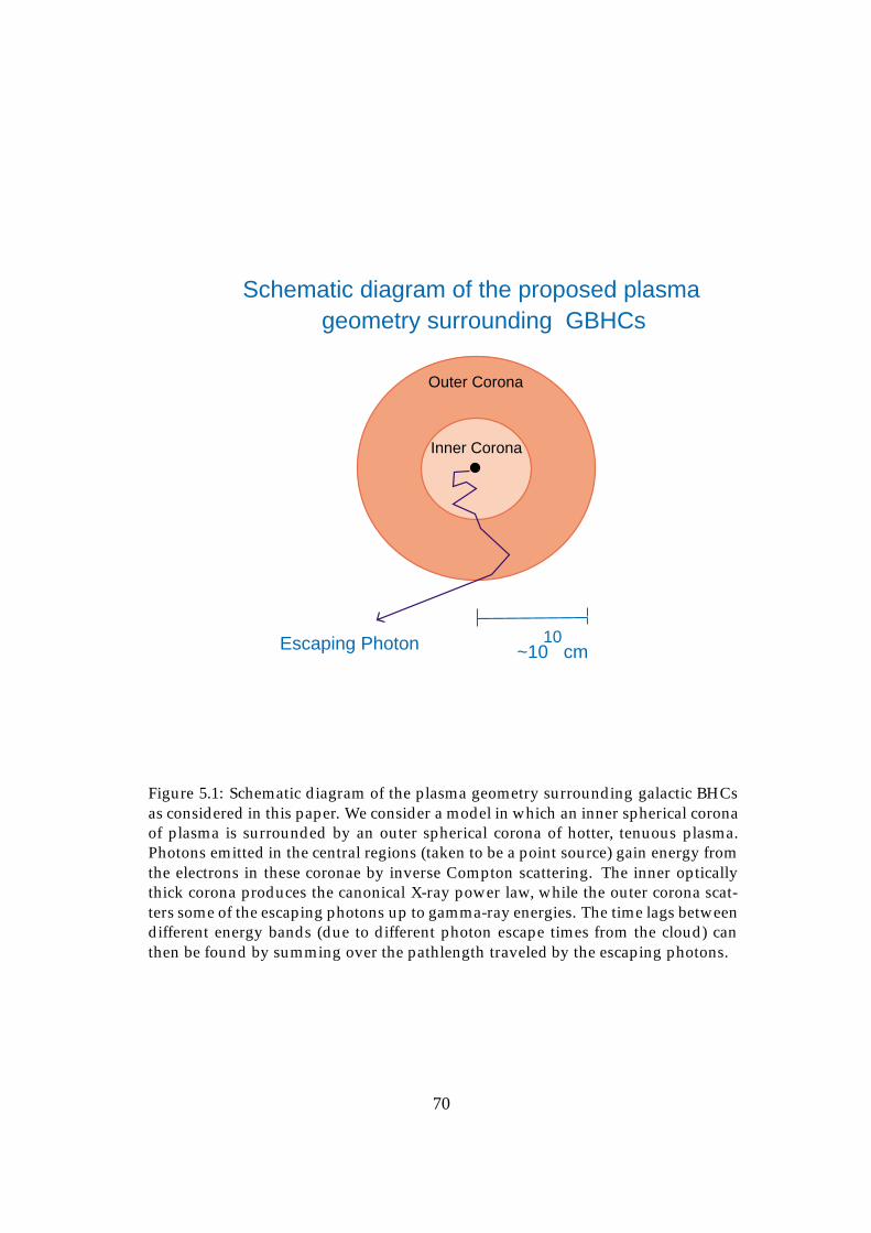
Schematic diagram of the proposed plasma geometry surrounding GBHCs

Escaping Photon

Outer Corona

Inner Corona

~10 cm10

Figure 5.1: Schematic diagram of the plasma geometry surrounding galactic BHCsas considered in this paper. We consider a model in which an inner spherical coronaof plasma is surrounded by an outer spherical corona of hotter, tenuous plasma.Photons emitted in the central regions (taken to be a point source) gain energy fromthe electrons in these coronae by inverse Compton scattering. The inner opticallythick corona produces the canonical X-ray power law, while the outer corona scat-ters some of the escaping photons up to gamma-ray energies. The time lags betweendifferent energy bands (due to different photon escape times from the cloud) canthen be found by summing over the pathlength traveled by the escaping photons.

70

simulates inverse Compton scattering of photons off relativistic Maxwellian electrons ina plasma of given electron temperature and optical depth. The evaluation of the mean-free-path integral (see Pozdnyakov, Sobol’ & Sunyaev 1983) assumes that the plasma ishomogeneous, that is, the electron temperature and the electron density are constant.The geometry of the coronal plasma is assumed to be spherically symmetric, with thesource of photons at the centre of a plasma cloud. To investigate the MCS model, theplasma is divided into a shell and a spherical core. The plasma in both of these regionsis homogeneous, but the two regions have different temperatures and optical depths(figure 5.1). The cloud is illuminated by a central source of blackbody photons withinjection taken to be a delta function in time. In the simulations the outermost radius ofthe cloud is fixed to be 1.0 light second across.

The photons are injected at the centre after being assigned an energy drawn from ablackbody distribution as well as some initial direction of propagation. The injectionis isotropic. Knowing the mean-free-path, the distance to the first scattering point isobtained using Eq. 2.17. All three components of the position vector of the photon arestored, as are all three components of the direction of propagation vector. After the pho-ton is moved to the location of the scattering event (Eq. 2.19), but before the scatteringevent itself is modeled, the distance of the photon from the origin at the centre of thesphere is determined. This distance is compared to the radius of the inner corona, andif it is larger the photon must have crossed the boundary between the inner and theouter corona (that is, from the core to the shell). When a photon crosses this boundary,it is brought back along its path to the boundary, and (without changing its directionof propagation) a new mean free path is calculated based on the temperature and opti-cal depth of the outer corona. A new distance to a scattering point is drawn using thisnew mean-free-path and the photon enters the outer corona. Because the optical depthof the outer corona is low, the mean-free-path of the photons is very large. Therefore,most photons in the simulation propagate through the shell and escape without scat-tering. Escape is determined by again comparing the distance of the photon from theorigin to the outer radius of the shell. If the photon does scatter after entering the outercorona, a routine will determine if the photon is heading back towards the inner cloudand will re-enter the core. If it does, the distance from the photon’s present locationto the boundary is determined by solving a simple quadratic equation. The photonsthat subsequently re-enter the inner corona are again placed on the boundary, and theoptical depth and temperature are reset to their values in the inner cloud. The originalmean-free-path is used to draw a new distance to a scattering point, and the simula-tion proceeds. A photon that escapes from the plasma cloud is binned in energy, and a

71

new photon injected. In this way, after many photon trajectories have been followed aspectrum is obtained.

The pathlength travelled by each photon is tracked and summed to give the totaldistance traveled (in units normalized to the outer cloud radius). This is convertedinto an escape time from the cloud which is binned to give the light curves, that is, theintensity in various bands as a function of time. These light curves are therefore Green’sfunctions in the sense that they represent the response of the system to a delta-functionsource term.

The Fourier time lags are then produced from the light curves (see Section 5.4) usingthe Fast Fourier Transform (FFT) routines in IDL. (Results were checked with thoseobtained numerically by Kazanas, Hua & Titarchuk (1997).)

5.3 Results: spectra

Figure 5.2 shows the single-temperature (isothermal) coronal Comptonized spectrumproduced by a spherical homogeneous cloud of plasma of optical depth � = 2:39 andelectron temperature of kTe = 76:7 keV (dotted line). Figure 5.2 also shows the spectrumproduced by assuming the MCS model (solid line). The inner cloud parameters are thesame as in the single cloud case, and the outer cloud is of effective optical depth � = 0:06

and electron temperature kTe = 396 keV. These temperatures and optical depths arethe best fit values (as determined by MCS) to the spectra obtained by CGRO BATSE-COMPTEL observations of Cyg X-1 taken when it was in the low state. Also shown isthe injected source spectrum which is assumed to be a blackbody distribution of tem-perature 130 eV. The ratio of radius of the inner cloud to the outer cloud radius is a freeparameter, but the overall energy spectrum is insensitive to this. Here it is fixed to be0:1.

In both cases, photons gain energy by Comptonization as they diffuse through thecloud, producing a power law spectrum. It can be seen from figure 5.2 that the single-temperature corona spectrum has a cutoff at below 1.0 MeV, while the multi-temperaturemodel produces substantial numbers of photons with energies in the MeV range. Thishigh energy excess is due to the photons that are scattered up to gamma-ray energies inthe high temperature outer cloud.

Note that the X-ray power law part of the spectrum has the same slope between2�100 keV for both the single and double corona models. This is required as the canon-ical single corona model accounts well for the X-ray part of the spectrum. But while

72

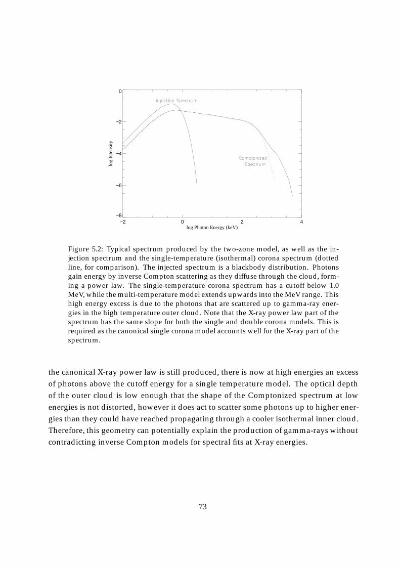
−2 0 2 4log Photon Energy (keV)

−8

−6

−4

−2

0

log

Inte

nsity

Figure 5.2: Typical spectrum produced by the two-zone model, as well as the in-jection spectrum and the single-temperature (isothermal) corona spectrum (dottedline, for comparison). The injected spectrum is a blackbody distribution. Photonsgain energy by inverse Compton scattering as they diffuse through the cloud, form-ing a power law. The single-temperature corona spectrum has a cutoff below 1.0MeV, while the multi-temperature model extends upwards into the MeV range. Thishigh energy excess is due to the photons that are scattered up to gamma-ray ener-gies in the high temperature outer cloud. Note that the X-ray power law part of thespectrum has the same slope for both the single and double corona models. This isrequired as the canonical single corona model accounts well for the X-ray part of thespectrum.

the canonical X-ray power law is still produced, there is now at high energies an excessof photons above the cutoff energy for a single temperature model. The optical depthof the outer cloud is low enough that the shape of the Comptonized spectrum at lowenergies is not distorted, however it does act to scatter some photons up to higher ener-gies than they could have reached propagating through a cooler isothermal inner cloud.Therefore, this geometry can potentially explain the production of gamma-rays withoutcontradicting inverse Compton models for spectral fits at X-ray energies.

73

5.4 Results: time lags

When IC scattering is the process responsible for producing high energy photons, therewill be a ‘hard’ time lag between the photons at high and low energies. To see this,consider the rate of energy gain by soft photons in a plasma of constant density. Theenergy gain (initially) increases exponentially with time (see Eq. 1.46), so if one imag-ines a burst of photons within a corona, the photons that escape promptly are of lowenergy. They have not had time to be scattered up to high energies. At progressivelylater times, the photons observed escaping will have progressively higher energies, sim-ply because they will have undergone more scattering events on average. Consider twonarrow energy bands, E1 and E2. If photons are injected at time zero with energy E0

then photons will be in energy band E1 at time t1, and some time after that will be inenergy band E2 at time t2. Because the energy gain is exponential, one has the equationsE1 = E0 exp(4yt1) and E2 = E0 exp(4yt2). A simple estimate for the time lag is then thedifference between the two times t2 � t1 =

14y (ln(E2=E0)� ln(E1=E0)), or 1

4y ln(E2=E1).The photon time lags between two different energy bands essentially represent the

difference in photon pathlength (or escape time) between bands; photons in the higherenergy bands tend to have undergone more scattering events, and therefore have trav-eled further in order to escape the corona. In fixing the two energy bands, one is effec-tively choosing an average number of scattering events.

Time lags can be studied by means of Fourier transforms, resulting in a plot of timelag verses Fourier frequency. Time lags in the X-ray are indeed observed from galacticBHCs, however interpretation of the situation is not straightforward, because the formof the lags is not consistent with a simple homogeneous corona model. The time lagscreated by Comptonization in a homogeneous and isothermal corona are predicted tobe constant with Fourier frequency f , whereas the observed lags are typically close tof�1.

If a spherical corona has a r�1 radial density profile, and is illuminated from thecentre, it has been shown (Kazanas, Hua, & Titarchuk 1997) that time lags of a formsimilar to those observed can be obtained. This is because photons scattering at a rangeof radii introduce a range of timescales for escape from the corona. However, Nowak etal. (1999) has considered a similar geometry, except that the corona is illuminated fromthe outside by soft photons from a surrounding accretion disk. They have found thatthe resulting time lags are constant with Fourier frequency, similar to the homogeneouscase. Clearly how the illumination of the corona occurs can have a profound effect onthe form of the resulting time lags.

74

If the lags are indeed produced by the scattering of photons through the corona,one would expect the time lag to be proportional to the number of scattering eventsmultiplied by the average time between scattering events. The number of scatteringevents in an optically thin plasma is of the order of the optical depth � , and the averagetime between scattering events is the radius of the corona divided by � and the speed oflight, Rc=(�c), which gives a number of � 10�3sec. The magnitude of the observed timelags at low frequencies on the other hand can be up to 0:1 s. This is accounted for in theKazanas, Hua, & Titarchuk model by allowing the outer radius of the corona to be ofthe order of a light-second, even though it is unclear how the corona can be heated tohigh temperatures at large distances from the central regions.

Another model that attempts to account for spectral and timing data is due to Pouta-nen & Fabian (1999). In their model the corona consists of a number of flares that moveaway from the disk surface as the flare occurs. The motion away from the disk causesthe spectrum to become harder as time progresses, causing lags between the soft andhard photons. The magnitude of the lag is of the same order of the time-scale for the lifeof the flare.

There exists another statistic for variability called coherence (see Vaughan & Nowak1997). X-ray lags are observed to have a coherence of one, meaning that they are welldescribed by a linear transfer function between the light curves in each band. Howeverit is not clear that multiple flares on the surface of an accretion disk preserve coherence.If the response of the scattering medium is non-linear the coherence is no longer one.The coherence of static Compton coronae is equal to one, however any fluctuation in theparameters of the corona (as might be required to account for the observed root-mean-squared variability) destroys coherence.

The third model attempting to account for time lags postulates the propagation ofwaves within the accretion disk (Misra 2000). Propagation models, besides requiringvery slow propagation speeds, have been criticised by Maccarone, Coppi & Poutanen(2000) as not being consistent with the observed cross-correlation function between en-ergy bands in the soft X-rays. The r�1 corona model of Kazanas, Hua & Titarchuk alsoseems unable to account for the behaviour of the cross-correlation function.

The form of the time lags with Fourier frequency seems very similar in both the hardand soft states, especially in the case of Cyg X-1 (Pottschmidt et al 2000). Models thatdepend on geometry for producing time lags have difficulty accounting for why thisshould be so, since state transitions are thought to (possibly) be due to the size of thecorona changing with respect to the disk. The lags from neutron star systems are alsosimilar in form to those from systems thought to contain black holes (Poutanen 2000).

75

To date, there is no theoretical model that can account for all of the spectral and timingproperties of accreting compact objects.

The time lags between two energy bands can be found by Fourier transforming thelight curves in the high and low energy bands (van der Klis et al. 1987, Miyamoto et al.1988). If the number of counts (photons) in time bin k is c(1)k for one light curve, and c

(2)k

for the light curve in the other energy band, the discrete Fourier transform of each lightcurve gives two quantities,

FT (c(1)k ) � a

(1)j and FT (c

(2)k ) � a

(2)j : (5.1)

Here the subscript j is related to the Fourier frequency.The discrete Fourier transforms of the light curves a1j and a2j are then used to form

a quantity called the complex cross power spectrum (CPS). This is done by multiplyingthe complex Fourier amplitudes from the low-energy band with the complex-conjugateof the complex Fourier amplitudes from the high-energy band,

CPSj � (a(2)j )�

a(1)j : (5.2)

(Here the star denotes complex conjugate of the complex number a(2)j ). The CPS is com-plex, and so can be thought of as a vector in the real and imaginary plane. The angle be-tween this vector and the real axis will be the phase lag between the two energy bands.This is performed by taking the imaginary part of the complex cross power spectrumCPSj and then dividing by its real part. Finally, the arctangent of the result is taken tofind the phase lag between bands as a function of Fourier frequency,

� = arctan

"Im(CPSj)

Re(CPSj)

#: (5.3)

Dividing the phase lag � by 2�f (where f is the Fourier frequency) then gives the hardtime lag curve as a function of Fourier frequency.

This technique has been used to investigate the time variability of galactic BHCs (forexample, van der Hooft et al. 1999). As discussed above, Kazanas, Hua & Titarchuk(1997) have used this method to investigate the effect of density gradients in the Comp-tonizing plasma, and Bottcher and Liang (1998, 1999) have attempted to determine thelocation of the photon source with respect to the plasma. These authors found that thetime lag curve is sensitive to variations in electron density.

Here, this method is used to determine the effect a density discontinuity of the typesuggested by MCS has on the time lag curve. The radius of the inner cloud is assumedto be a free parameter, while the outer radius is fixed at one light second. Changing

76

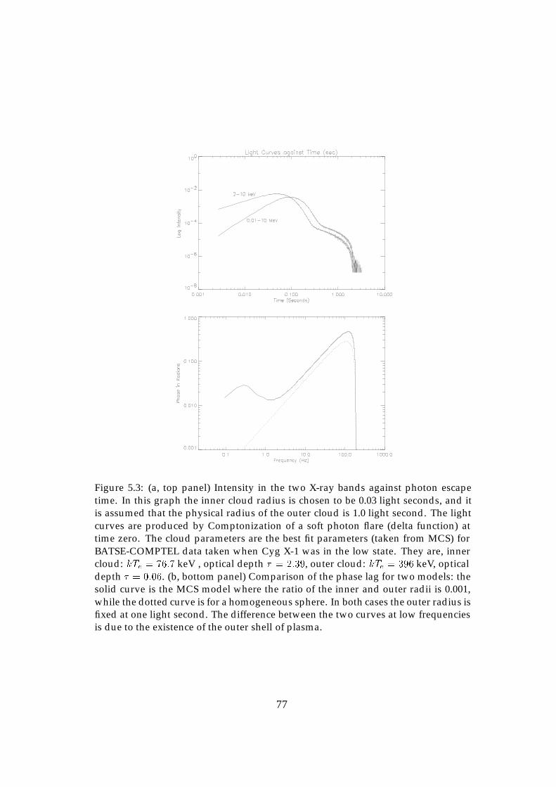
Figure 5.3: (a, top panel) Intensity in the two X-ray bands against photon escapetime. In this graph the inner cloud radius is chosen to be 0.03 light seconds, and itis assumed that the physical radius of the outer cloud is 1.0 light second. The lightcurves are produced by Comptonization of a soft photon flare (delta function) attime zero. The cloud parameters are the best fit parameters (taken from MCS) forBATSE-COMPTEL data taken when Cyg X-1 was in the low state. They are, innercloud: kTe = 76:7 keV , optical depth � = 2:39, outer cloud: kTe = 396 keV, opticaldepth � = 0:06. (b, bottom panel) Comparison of the phase lag for two models: thesolid curve is the MCS model where the ratio of the inner and outer radii is 0.001,while the dotted curve is for a homogeneous sphere. In both cases the outer radius isfixed at one light second. The difference between the two curves at low frequenciesis due to the existence of the outer shell of plasma.

77

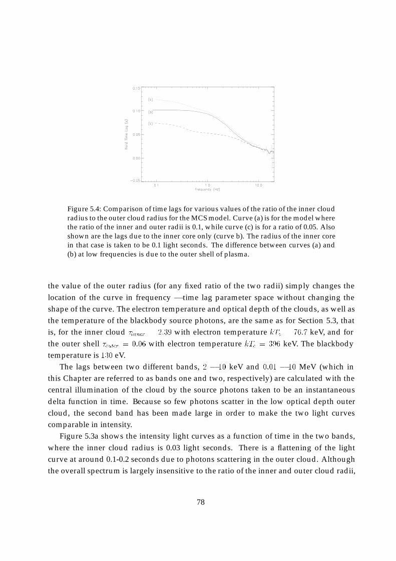
Figure 5.4: Comparison of time lags for various values of the ratio of the inner cloudradius to the outer cloud radius for the MCS model. Curve (a) is for the model wherethe ratio of the inner and outer radii is 0.1, while curve (c) is for a ratio of 0.05. Alsoshown are the lags due to the inner core only (curve b). The radius of the inner corein that case is taken to be 0.1 light seconds. The difference between curves (a) and(b) at low frequencies is due to the outer shell of plasma.

the value of the outer radius (for any fixed ratio of the two radii) simply changes thelocation of the curve in frequency � time lag parameter space without changing theshape of the curve. The electron temperature and optical depth of the clouds, as well asthe temperature of the blackbody source photons, are the same as for Section 5.3, thatis, for the inner cloud �inner = 2:39 with electron temperature kTe = 76:7 keV, and forthe outer shell �outer = 0:06 with electron temperature kTe = 396 keV. The blackbodytemperature is 130 eV.

The lags between two different bands, 2 � 10 keV and 0:01 � 10 MeV (which inthis Chapter are referred to as bands one and two, respectively) are calculated with thecentral illumination of the cloud by the source photons taken to be an instantaneousdelta function in time. Because so few photons scatter in the low optical depth outercloud, the second band has been made large in order to make the two light curvescomparable in intensity.

Figure 5.3a shows the intensity light curves as a function of time in the two bands,where the inner cloud radius is 0.03 light seconds. There is a flattening of the lightcurve at around 0.1-0.2 seconds due to photons scattering in the outer cloud. Althoughthe overall spectrum is largely insensitive to the ratio of the inner and outer cloud radii,

78

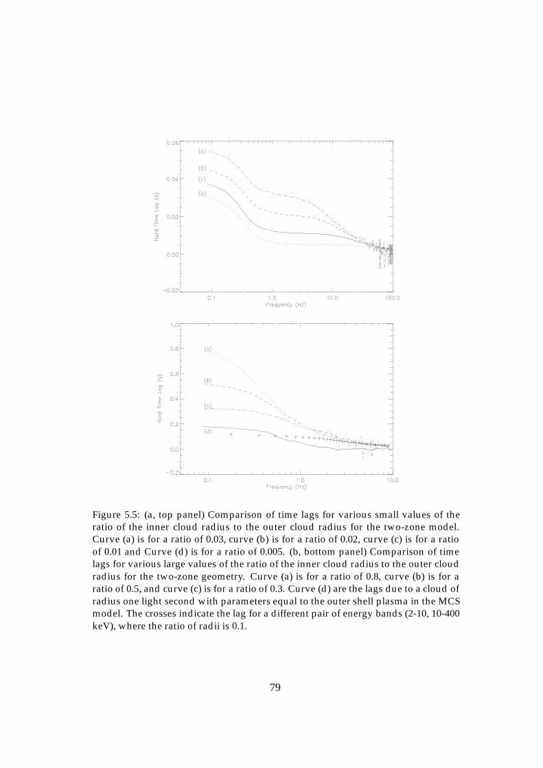
Figure 5.5: (a, top panel) Comparison of time lags for various small values of theratio of the inner cloud radius to the outer cloud radius for the two-zone model.Curve (a) is for a ratio of 0.03, curve (b) is for a ratio of 0.02, curve (c) is for a ratioof 0.01 and Curve (d) is for a ratio of 0.005. (b, bottom panel) Comparison of timelags for various large values of the ratio of the inner cloud radius to the outer cloudradius for the two-zone geometry. Curve (a) is for a ratio of 0.8, curve (b) is for aratio of 0.5, and curve (c) is for a ratio of 0.3. Curve (d) are the lags due to a cloud ofradius one light second with parameters equal to the outer shell plasma in the MCSmodel. The crosses indicate the lag for a different pair of energy bands (2-10, 10-400keV), where the ratio of radii is 0.1.

79

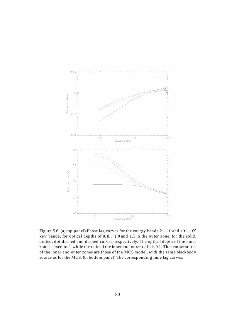
Figure 5.6: (a, top panel) Phase lag curves for the energy bands 2� 10 and 10� 100

keV bands, for optical depths of 0; 0:5; 1:0 and 1:5 in the outer zone, for the solid,dotted, dot-dashed and dashed curves, respectively. The optical depth of the innerzone is fixed to 2, while the ratio of the inner and outer radii is 0.1. The temperaturesof the inner and outer zones are those of the MCS model, with the same blackbodysource as for the MCS. (b, bottom panel) The corresponding time lag curves.

80

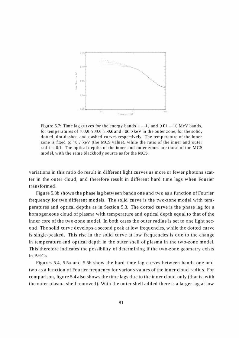
Figure 5.7: Time lag curves for the energy bands 2 � 10 and 0:01� 10 MeV bands,for temperatures of 100:0; 200:0; 300:0 and 400:0 keV in the outer zone, for the solid,dotted, dot-dashed and dashed curves respectively. The temperature of the innerzone is fixed to 76:7 keV (the MCS value), while the ratio of the inner and outerradii is 0.1. The optical depths of the inner and outer zones are those of the MCSmodel, with the same blackbody source as for the MCS.

variations in this ratio do result in different light curves as more or fewer photons scat-ter in the outer cloud, and therefore result in different hard time lags when Fouriertransformed.

Figure 5.3b shows the phase lag between bands one and two as a function of Fourierfrequency for two different models. The solid curve is the two-zone model with tem-peratures and optical depths as in Section 5.3. The dotted curve is the phase lag for ahomogeneous cloud of plasma with temperature and optical depth equal to that of theinner core of the two-zone model. In both cases the outer radius is set to one light sec-ond. The solid curve develops a second peak at low frequencies, while the dotted curveis single-peaked. This rise in the solid curve at low frequencies is due to the changein temperature and optical depth in the outer shell of plasma in the two-zone model.This therefore indicates the possibility of determining if the two-zone geometry existsin BHCs.

Figures 5.4, 5.5a and 5.5b show the hard time lag curves between bands one andtwo as a function of Fourier frequency for various values of the inner cloud radius. Forcomparison, figure 5.4 also shows the time lags due to the inner cloud only (that is, withthe outer plasma shell removed). With the outer shell added there is a larger lag at low

81

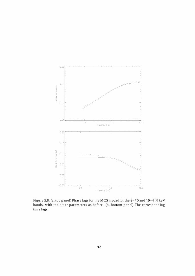
Figure 5.8: (a, top panel) Phase lags for the MCS model for the 2�10 and 10�100 keVbands, with the other parameters as before. (b, bottom panel) The correspondingtime lags.

82

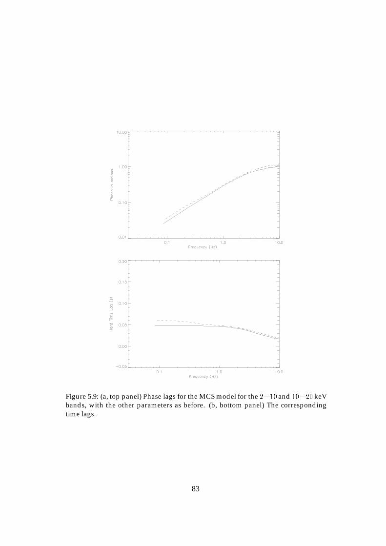
Figure 5.9: (a, top panel) Phase lags for the MCS model for the 2�10 and 10�20 keVbands, with the other parameters as before. (b, bottom panel) The correspondingtime lags.

83

frequencies than for the inner cloud alone. This is the key difference between simplespherical corona models and the multi-temperature model due to MCS.

Figure 5.5a shows that for small inner-radius values, the lags become almost con-stant at high frequencies as the inner radius is made small, but there is still a peakat low frequencies. For large inner-radius values (figure 5.5b), one is seeing the innercloud/core only, as fewer photon scatter in the relatively smaller outer cloud/shell.Figure 5.5b also shows the lags due to a spherical corona with electron temperatureand optical depth equal to that of the outer cloud/shell in the two-zone model. This isequivalent to making the inner cloud radius and optical depth approach zero.

The crosses in figure 5.5b show the lags for a different pair of energy bands (2 � 10,10 � 400 keV, where the ratio of radii is 0.1). Because these bands do not extend upto gamma-ray energies, fewer high energy photons from the outer corona have con-tributed to the time lag curve. The lags are therefore almost constant with frequency asone is essentially seeing just the inner corona. In this case the lags tell us little about theouter corona.

It is possible that the various time lag curves could be used to determine the ratio ofthe inner and outer radii, as well as set the overall scale of the corona. Given the tem-peratures and optical depths (from spectral modeling) of the inner and outer coronae,the shape of the hard time lag curve determines the ratio of the inner and outer radii,while the position of the hard time lag curve in the frequency � time lag parameterspace determines the magnitude of the outer radius. Thus if the optical depths and thevalues of the radii are known, then the density of the corona is known, and one can inprinciple know all the physical parameters of the corona (in the context of the two-zonemodel). It is also possible that the outer radius can be found from other criteria, perhapsby identifying the break in the power spectral density of a light curve with the value ofthe outer radius as suggested by Bottcher & Liang (1998).

Figure 5.6 investigates variations in the optical depth of the outer shell. Here, op-tical depth parameters different from those of the MCS model have been chosen. Forthe inner cloud, � = 2:0 (solid line), while the optical depth of the outer shell is setto 0:5; 1:0 and 1:5 for the dotted curve, dot-dashed curve and the dashed curve re-spectively. Again, the magnitude of the time lag increases at low Fourier frequenciescompared to the no-shell case. The time lag curve seems to be reasonably sensitive tovariations in the optical depth of the outer shell.

Figure 5.7 investigates variations in the temperature of the outer shell. Here, theoptical depth of the inner and outer clouds are chosen to be those of the MCS model.For the inner cloud, the temperature is 76:7 keV, while the temperature of the outer shell

84

is set to 100:0; 200:0; 300:0 and 400:0 keV for the solid curve, dotted curve, dot-dashedcurve and the dashed curve respectively. At the lowest temperature, the time lag curveis essentially formed due to scattering in the inner cloud only, since photons are notscattered up to energies greater than � 100:0 keV and the light curves closely resemblethose for the case of no outer cloud at all. As the outer cloud temperature increases,there is a rise in the curve at low Fourier frequencies (0:1 � 0:2 Hz). Overall, thereis not much variation in the time lag curve with temperature in the outer cloud, withvariations in optical depth (figure 5.6) having the larger influence on the time lags.

A more exact treatment of the curves in Figure 5.7 would begin by noting that sincethe scattering cross-section depends on temperature as well as density, to determine theeffect of temperature only one should also vary/scale the density of the outer corona soas to keep the probability of scattering constant. Since the cross-section decreases withincreasing temperature, the density in such a simulation would have to be increased tomaintain the same scattering probability.

Figures 5.8 and 5.9 investigate the choice of different energy bands on the phase andtime lags, for the MCS model. Figure 5.8 shows the lag between the 2� 10 and 10� 100

keV bands, while Figure 5.9 shows the lag between the 2�10 and 10�20 keV bands. Thesolid line is for the inner sphere only, and the dashed curve is for both the inner sphereand outer shell. There is an increase in the time lag curve at low Fourier frequencies ofabout 0:02 seconds, for both the figures. However the maximum time lag is larger inthe case where the high energy band extends up to higher energies (10� 100, figure 5.8)than it is when the high energy band is 10� 20 (figure 5.9). This is because it takes someextra time to scatter photons up to energies approaching 100 keV.

5.5 Conclusion

This Chapter has investigated in detail the two-zone model for the geometry of theplasma surrounding BHCs. In particular, this study has calculated the full spectrumproduced by this model using a Monte Carlo simulation, as well as the time depen-dent light curves produced by Comptonization of a soft radiation flare at time zero,and the hard time lag curve between different energy bands. This is the first time thelight curves and the hard time lags from a plasma with the two-zone geometry havebeen investigated numerically. It is found that Monte Carlo investigation of photontime lags between different energy bands can possibly be used to constrain this multi-temperature geometry for the accretion disk corona around galactic BHCs.

85

The energy spectrum is largely insensitive to the values of the radii used for theinner and outer clouds, as in general a Comptonized spectrum is sensitive only to thetemperature and optical depth of the plasma (and the initial photon distribution if theplasma is optically thin). However, it is found that the time lag curve between energybands is sensitive to the ratio of the two radii. This is the main result of the work in thisChapter; a sharp rise in the time lag curve at low Fourier frequencies is the temporalsignature of the MCS model.

Variations in the optical depth and the temperature of the outer shell were inves-tigated. The magnitude of the lag at low Fourier frequencies increases with both in-creasing optical depth and increasing temperature. However, it is seen that the time lagcurve is more sensitive to variations in the optical depth (figure 5.6) than variations intemperature (figure 5.7). This may be due to the choice of energy bands, which werewide enough to bin photons regardless of whether those photons scattered in 100:0 keVplasma or 400:0 keV plasma.

Variations in the choice of energy bands were also investigated. The magnitude ofthe lags is larger when one of the energy bands extends up to higher energies, how-ever judging from these results (figure 6.6 and figure 6.7) the dependence on the energybands is not strong. A rise in the phase/time lag curve at low Fourier frequencies oughtto be a general prediction for two-zone corona models with a hotter outer shell, even ifthe energy bands are somewhat different from those chosen here.

MCS also consider the case where bremsstrahlung photons from the tenuous outercorona are a significant spectral component. However, if the bremsstrahlung photonflux is stationary, then this component will make no contribution to the Fourier trans-form of the light curves, and therefore no contribution to the time lag curve. This willbe the case as long as any fluctuations in the bremsstrahlung flux are small comparedto the amplitude of the central Comptonized pulse. Similarly, any time independentprocesses such as electron-positron annihilation should not contribute significantly tothe time lags.

Thus the time delay or lag can be used to determine the overall size of the coronaand the ratio of the inner and outer radii, if this two-component corona geometry exists.This information combined with values for the optical depth obtained from spectralmodeling can then tell us the overall density of the corona. Such a result would thengive us all the physical parameters of the plasma cloud.

Observationally, the phase lag curve for galactic BHCs is typically constant withFourier frequency (Miyamoto 1988). If the rise feature is unobserved, the absence ofthe feature could in theory place a constraint on the optical depth (and perhaps the

86

temperature) of any outer corona. If a two-zone model is found to be unviable usingthe time lags technique, other models for gamma-ray production will then be required.

87

References

Bisnovatyi-Kogan, G. S. & Blinnikov, S. I. 1976, Soviet Astron. Lett., 2, 191Bottcher, M. & Liang, E. P. 1998, ApJ, 506, 281Bottcher, M. & Liang, E. P. 1999, ApJ, 511, L37Dove, J. B., et al. 1997, ApJ, 487, 759Esin, A. A., et al. 1998, ApJ, 505, 854van der Hooft, F., et al. 1999, ApJ, 513, 477Johnson, W. N., et al. 1993, A & AS, 97, 21van der Klis, M., et al. 1987, ApJ, 319, L13Kazanas, D., Hua, X. M. & Titarchuk, L. G. 1997, ApJ, 480, 735Li, H., Kusunose, M. & Liang, E. P. 1996, ApJ, 460, L29Maccarone, T. J., Coppi, P. S. & Poutanen, J. 2000, ApJ, 537, L107Misra, R. 2000, ApJ, 529, L95Miyamoto, S., et al. 1988, Nature, 336, 450Moskalenko, I. V., Collmar, W. & Schonfelder, V. 1998, ApJ, 502, 428Nowak, M. A., et al. 1999, ApJ, 515, 726Pottschmidt, K., et al. (in press) astro-ph/0008059Poutanen, J. & Fabian, A. C. 1999, MNRAS, 306, L31Poutanen, J. 2000, “X-ray Astronomy 1999” meeting, astro-ph/0002505Pozdnyakov, L. A., Sobol, I. M. & Sunyaev, R. A. 1983, Ap. & Space Sci. Reviews, 2, 189.Sunyaev, R. A. & Titarchuk, L. G. 1980, A&A, 86, 121Vaughan, B. A. & Nowak, M. A. 1997, ApJ, 474, L43

88

Chapter 6

Compton scattering in bulk accretionflows

Inspired by previous studies of bulk motion Comptonization in converging accretionflows, the techniques discussed in Chapter 3 are applied here to the study of scatteringin bulk motion accretion flows in both one and two dimensions.

Firstly, the case of line photon scattering in the accretion column of a magnetisedwhite dwarf star (1D) is considered, with the resulting spectra presented for variousinclination angles, accretion rates, and Cyclotron cooling rates in the post-shock region.Spectra as a function of inclination angle are also obtained, so that beaming of photonsby the inhomogeneous column can be investigated.

Secondly, the case of Comptonization in a rotating torus geometry (2D) is consid-ered, which is a first attempt at considering scattering in an orbiting accretion disk-likestructure. Different photon injection spectra (a line, a power law and a blackbody) areinvestigated for different values of electron momentum. It is found that for a reason-able optical depth and electron momentum, lines can be significantly broadened byrotational Compton scattering.

6.1 1D: Accretion column

6.1.1 Accretion column in magnetic white dwarf stars

Magnetised white dwarf stars that accrete material from a binary companion star aresources of X-rays. After spilling out of the Roche lobe of the companion, the accreting

89

material is channeled by the magnetic field lines of the white dwarf into an accretioncolumn which falls onto the pole of the white dwarf star.

A standing shock is formed near the base of the accretion column where the energyassociated with free-fall is thermalised. The shock temperature is

kTs = 16 (M=0:5M�)(R=109cm)�1 keV (6.1)

for a white dwarf of 0.5 solar masses and radius 109cm (Frank, King & Raine 1985).Observational evidence for a temperature distribution in the post-shock plasma waspresented by Ishida, Mukai & Osborne (1994). There are also expected to be velocityand density gradients in the post-shock region, which are predicted by hydrodynamicmodels of the accretion column (Aizu 1973, Wu, Chanmugam & Shaviv 1994).

Iron K� and K� lines have been observed, for instance in EX Hydrae (Ishida et al.1994). These are interpreted as being emitted by optically thin thermal plasma withinthe accretion column. The emissivity functions of Fe, Ar, S, Si and Mg have been stud-ied (Fujimoto & Ishida 1997) and are found to peak towards the base of the accretioncolumn, except for Fe which can be emitted at the shock.

White dwarf accretion columns can, for certain accretion rates, be sufficiently opti-cally thick to scatter large numbers of line photons. Here, a Monte Carlo technique isused to investigate line photons that have scattered in an accretion column with den-sity, temperature and velocity gradients. Spectra of escaping photons as a function ofinclination angle are also presented. The photon transport within the accretion columnis treated using the technique presented in Chapter 3.

6.1.2 Description of the numerical approach: column

The code developed for this application uses the Monte Carlo technique to simulate thescattering of line photons and free electrons in an accretion column of material, that isfalling onto a weakly magnetised white dwarf star. The accretion column is modeled asa cylinder of material above the white dwarf pole (see figure 6.1). Within the accretioncolumn, the density and velocity of the material above the shock are taken to be con-stants, while below the shock the density, velocity and temperature profiles are given byexpressions presented in Wu et al. 1994. As discussed above, these profiles also includecooling of the post-shock material due to cyclotron radiation and to Bremsstrahlungradiation. The profiles are tabulated in arrays, to be used as needed.

The parameters of the accreting plasma used here are given by the hydrodynamicmodel of Wu, Chanmugam & Shaviv (1994). These authors solved the one-dimensional

90

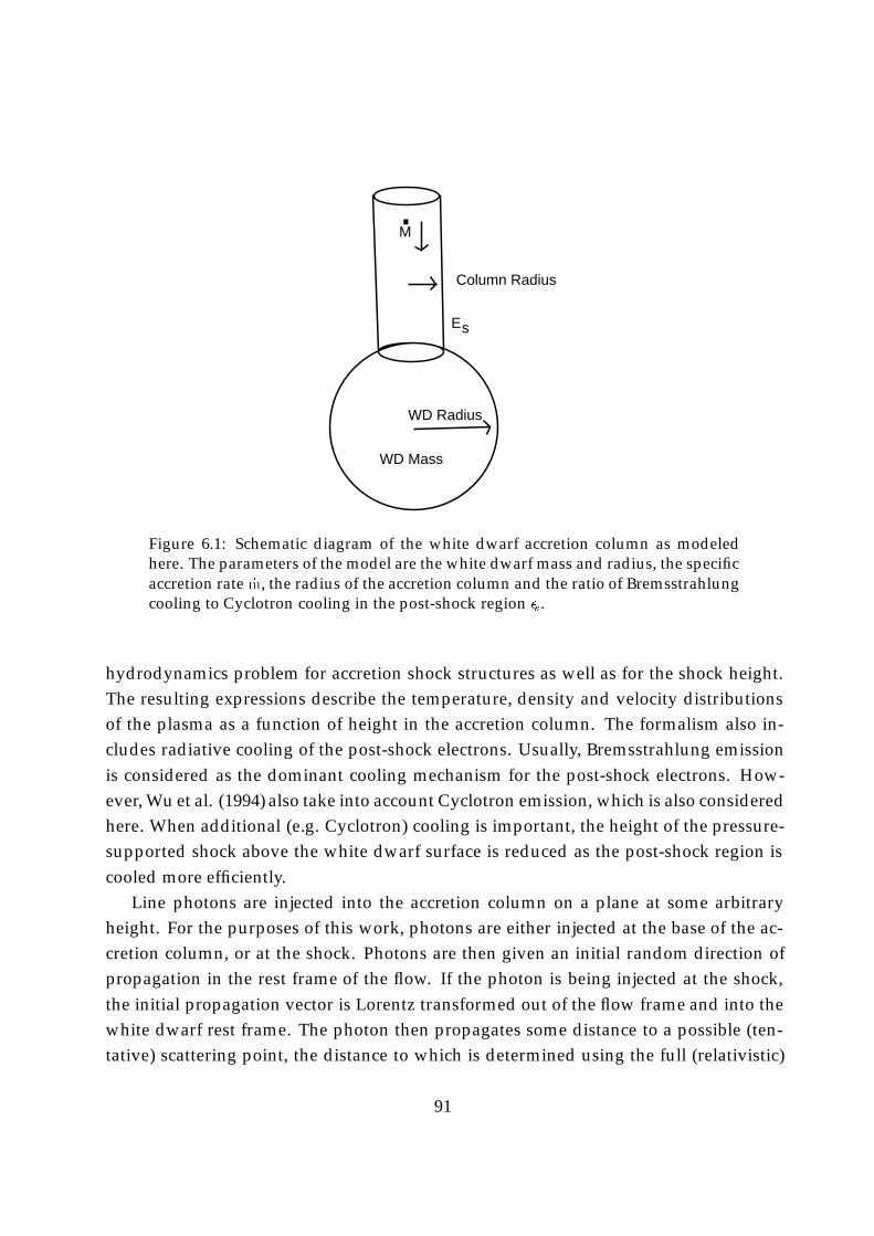
WD Mass

WD Radius

Column Radius

Es

M.

Figure 6.1: Schematic diagram of the white dwarf accretion column as modeledhere. The parameters of the model are the white dwarf mass and radius, the specificaccretion rate _m, the radius of the accretion column and the ratio of Bremsstrahlungcooling to Cyclotron cooling in the post-shock region �s.

hydrodynamics problem for accretion shock structures as well as for the shock height.The resulting expressions describe the temperature, density and velocity distributionsof the plasma as a function of height in the accretion column. The formalism also in-cludes radiative cooling of the post-shock electrons. Usually, Bremsstrahlung emissionis considered as the dominant cooling mechanism for the post-shock electrons. How-ever, Wu et al. (1994) also take into account Cyclotron emission, which is also consideredhere. When additional (e.g. Cyclotron) cooling is important, the height of the pressure-supported shock above the white dwarf surface is reduced as the post-shock region iscooled more efficiently.

Line photons are injected into the accretion column on a plane at some arbitraryheight. For the purposes of this work, photons are either injected at the base of the ac-cretion column, or at the shock. Photons are then given an initial random direction ofpropagation in the rest frame of the flow. If the photon is being injected at the shock,the initial propagation vector is Lorentz transformed out of the flow frame and into thewhite dwarf rest frame. The photon then propagates some distance to a possible (ten-tative) scattering point, the distance to which is determined using the full (relativistic)

91

Klein-Nishina cross-section and a variant of the non-linear transport technique intro-duced by Stern et al. 1995. As this is a rejection technique, not every tentative scatteringevent is accepted.

The original Stern rejection algorithm assumed a constant electron density. Here thealgorithm is modified to include an integration over the varying electron density (in thepost-shock region), but otherwise the algorithm is unchanged (see Chapter 3).

At a tentative scattering point the momentum vector of an electron is drawn froman isotropic Maxwellian distribution, whose temperature is given by the value of thetemperature profile at this point (read from the arrays of tabulated values). The electronmomentum vector is then Lorentz transformed out of the flow rest frame and into thewhite dwarf frame, using the velocity of the flow at the point. (The expression forLorentz transforming a vector can be found in, for instance, Hua 1997). This gives the’resultant’ electron momentum vector, in the sense that part is due to thermal motionand part is due to the bulk motion of the flow. Based on the electron and the photon,the rejection algorithm then decides whether to accept or reject the scattering event. Theprobability of accepting the event is determined using Eq. 3.13, which depends on thecross-section and the relative velocity between the electron and photon.

If a scattering event does take place, the energy shift of the photon, and the change inpropagation direction, are modeled according to the prescription given by Pozdnyakov,Sobol and Sunyaev (1983), again using the full Klein-Nishina cross-section.

Photons are followed until they escape from the accretion column, and are binned inenergy for a given viewing angle. Here viewing angles of 30� and 60� are investigated.Furthermore, all escaping photons are binned in angle. Photons that hit the white dwarfsurface are disregarded and do not contribute to the final spectrum.

The code inputs are the mass and radius of the white dwarf star, the specific accretionrate within the accretion column, the width of the accretion column, and the ratio ofCyclotron cooling to Bremsstrahlung cooling in the post-shock region. The code beingused in this Section is used here in a ’linear’ mode, so the value of the time step used bythe code does not effect the results (this also holds for the code discussed in Section 6.2).

The procedure just described treats both the photon transport and the photon scat-tering accurately. The full white dwarf code is presented in the appendix of this thesis.

6.1.3 Results

The spectra have been investigated for different accretion rates, viewing angles, photoninjection sites and cyclotron cooling ratios. The results are plotted in figures 6.2 - 6.6.

92

For all these figures, the radius of the accretion column was taken to be 10% of thewhite dwarf radius, while the mass and radius of the white dwarf were 0:5M� and109cm. For figures 6.2 - 6.4 the ratio of the Bremsstrahlung cooling timescale to theCyclotron cooling timescale at the shock, �s (as defined in Wu et al. 1994), is set to zero(Bremsstrahlung cooling only).

Figures 6.2a and 6.2b show spectra for a specific accretion rate of 4 g s�1cm�2 (solidlines), seen at 30� inclination (Figure 6.2a), and at 60� inclination from the axis of theaccretion column (Figure 6.2b). The photons are injected at the shock with an energy of6:7 keV in the rest frame of the accreting material. The dashed lines are the same exceptthe specific accretion rate is 40 g s�1cm�2.

Figures 6.3a and 6.3b are for the same parameters as figures 6.2a and 6.2b, excepthere the photon injection site is at the base of the accretion column.

To interpret figures 6.2 and 6.3, consider first those photons that scatter in the pre-shock material. In a homogeneous cold column, a typical spectrum consists of a doublepeaked structure, followed by a ‘plateau’ at lower energies, and a low energy tail. Whenthe photon injection site is located near the white dwarf, the backscattered photons ofthe second (lower energy) peak have a much greater chance of hitting the white dwarfsurface and being absorbed. The result is that the second peak gets is diminished asthe injection site approaches the surface. The resulting spectra have a strong first peak,in some cases a remnant of the second peak, and the plateau due to photons that havescattered subsequent times. This is superimposed on a very broad feature that is dueto those photons that have scattered in the post-shock material. Those photons thathave encountered hot electrons near the shock are upscattered to higher energies, whilephotons that scatter in the dense, cool material near the white dwarf surface can losesignificant amounts of energy. This results in broad wings that extend off to both higherand lower energies. Figures 6.2 show lines with the remnant of the backscattered peakbetween 6.7 keV and 6.5 keV. Because the photon injection site in Figures 6.3 is closerto the white dwarf surface, the backscatter peak is gone, and the peak at 6.7 keV joinssmoothly onto the plateau feature.

Figures 6.4a and 6.4b show the spectrum (the number of escaping photons) as afunction of the angle � � cos�1(�), where � = 1:0 corresponds to the direction along thecolumn away from the white dwarf, and � = �1:0 corresponds to the direction alongthe column towards the white dwarf. Figure 6.4a is for the parameters used in figure6.2, while Figure 6.4b is for the parameters used in figure 6.3. At higher accretion rates,more escaping photons are beamed down towards the white dwarf, especially if thephotons are injected at the base of the column (figure 6.4b).

93

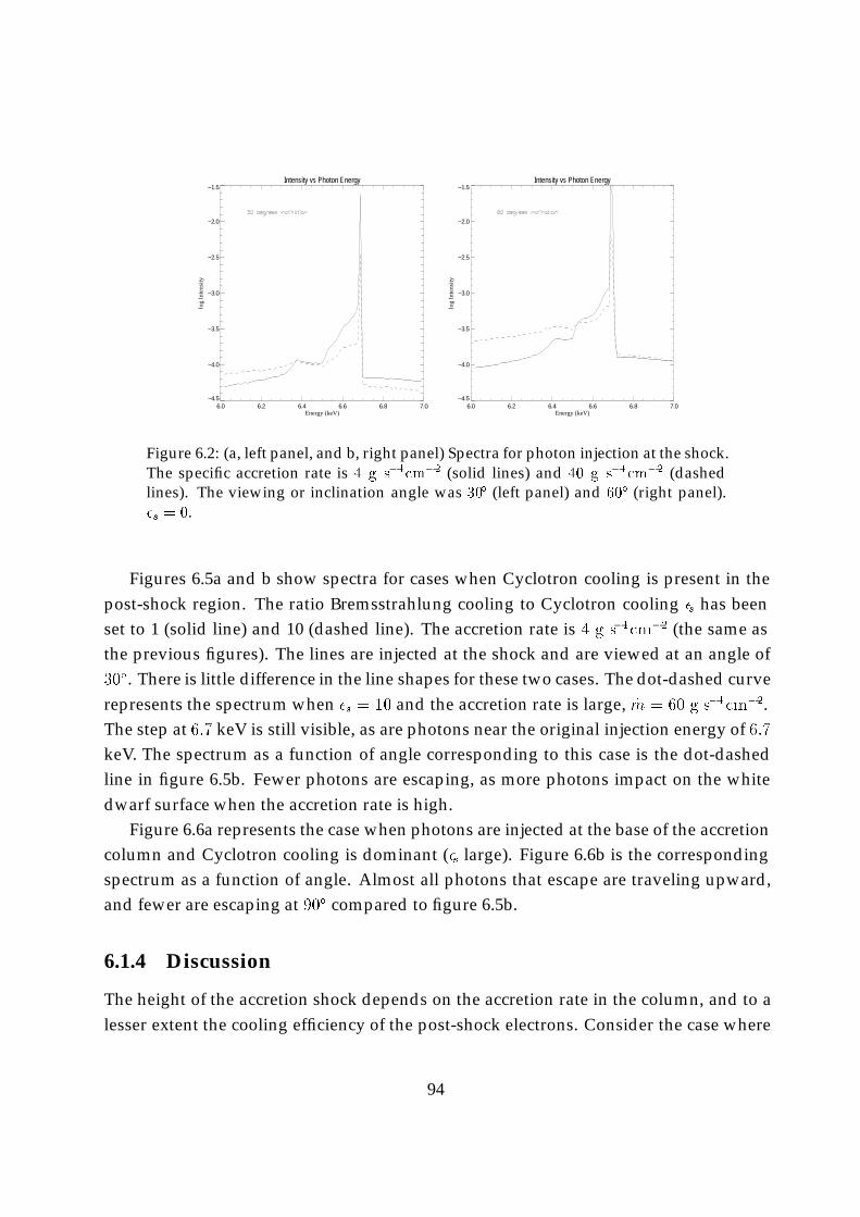
Intensity vs Photon Energy

6.0 6.2 6.4 6.6 6.8 7.0Energy (keV)

−4.5

−4.0

−3.5

−3.0

−2.5

−2.0

−1.5

log

Inte

nsity

Intensity vs Photon Energy

6.0 6.2 6.4 6.6 6.8 7.0Energy (keV)

−4.5

−4.0

−3.5

−3.0

−2.5

−2.0

−1.5

log

Inte

nsity

Figure 6.2: (a, left panel, and b, right panel) Spectra for photon injection at the shock.The specific accretion rate is 4 g s�1cm�2 (solid lines) and 40 g s�1cm�2 (dashedlines). The viewing or inclination angle was 30� (left panel) and 60� (right panel).�s = 0.

Figures 6.5a and b show spectra for cases when Cyclotron cooling is present in thepost-shock region. The ratio Bremsstrahlung cooling to Cyclotron cooling �s has beenset to 1 (solid line) and 10 (dashed line). The accretion rate is 4 g s�1cm�2 (the same asthe previous figures). The lines are injected at the shock and are viewed at an angle of30�. There is little difference in the line shapes for these two cases. The dot-dashed curverepresents the spectrum when �s = 10 and the accretion rate is large, _m = 60 g s�1cm�2.The step at 6:7 keV is still visible, as are photons near the original injection energy of 6:7keV. The spectrum as a function of angle corresponding to this case is the dot-dashedline in figure 6.5b. Fewer photons are escaping, as more photons impact on the whitedwarf surface when the accretion rate is high.

Figure 6.6a represents the case when photons are injected at the base of the accretioncolumn and Cyclotron cooling is dominant (�s large). Figure 6.6b is the correspondingspectrum as a function of angle. Almost all photons that escape are traveling upward,and fewer are escaping at 90� compared to figure 6.5b.

6.1.4 Discussion

The height of the accretion shock depends on the accretion rate in the column, and to alesser extent the cooling efficiency of the post-shock electrons. Consider the case where

94

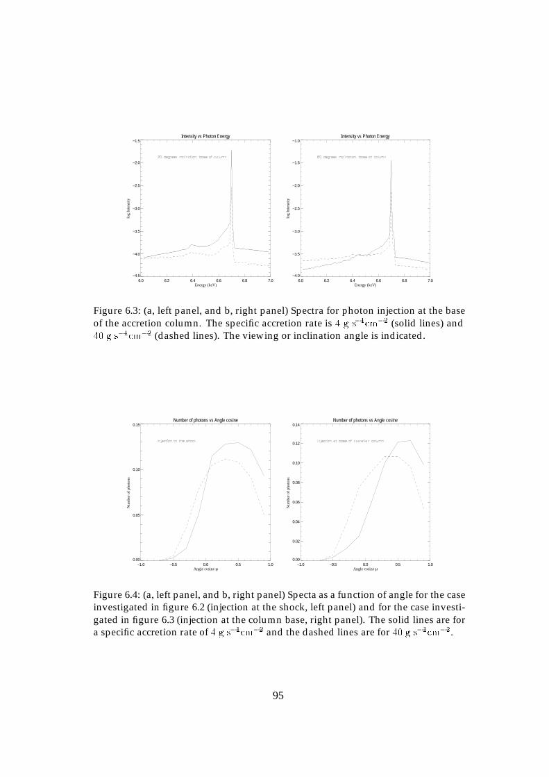
Intensity vs Photon Energy

6.0 6.2 6.4 6.6 6.8 7.0Energy (keV)

−4.5

−4.0

−3.5

−3.0

−2.5

−2.0

−1.5

log

Inte

nsity

Intensity vs Photon Energy

6.0 6.2 6.4 6.6 6.8 7.0Energy (keV)

−4.0

−3.5

−3.0

−2.5

−2.0

−1.5

−1.0

log

Inte

nsity

Figure 6.3: (a, left panel, and b, right panel) Spectra for photon injection at the baseof the accretion column. The specific accretion rate is 4 g s�1cm�2 (solid lines) and40 g s�1cm�2 (dashed lines). The viewing or inclination angle is indicated.

Number of photons vs Angle cosine

−1.0 −0.5 0.0 0.5 1.0Angle cosine µ

0.00

0.05

0.10

0.15

Num

ber

of p

hoto

ns

Number of photons vs Angle cosine

−1.0 −0.5 0.0 0.5 1.0Angle cosine µ

0.00

0.02

0.04

0.06

0.08

0.10

0.12

0.14

Num

ber

of p

hoto

ns

Figure 6.4: (a, left panel, and b, right panel) Specta as a function of angle for the caseinvestigated in figure 6.2 (injection at the shock, left panel) and for the case investi-gated in figure 6.3 (injection at the column base, right panel). The solid lines are fora specific accretion rate of 4 g s�1cm�2 and the dashed lines are for 40 g s�1cm�2.

95

Intensity vs Photon Energy

6.0 6.2 6.4 6.6 6.8 7.0Energy (keV)

−4.5

−4.0

−3.5

−3.0

−2.5

−2.0

−1.5lo

g In

tens

ityNumber of photons vs Angle cosine

−1.0 −0.5 0.0 0.5 1.0Angle cosine µ

0.00

0.05

0.10

0.15

Num

ber

of p

hoto

ns

Figure 6.5: (a, left panel, and b, right panel) Spectra for photon injection at the shock.The specific accretion rate is 4 g s�1cm�2 (solid and dashed lines). The viewingangle for all cases is 30�. �s = 1:0 for the solid line and 10:0 for the dashed line.The dot-dashed curve corresponds to an extreme case of large �s (10:0) and largeaccretion rate (60 g s�1cm�2). The right panel shows the corresponding spectra as afunction of angle for the solid line, dashed line and the dot-dashed case.

Intensity vs Photon Energy

6.0 6.2 6.4 6.6 6.8 7.0Energy (keV)

−4.0

−3.5

−3.0

−2.5

−2.0

−1.5

log

Inte

nsity

Number of photons vs Angle cosine

−1.0 −0.5 0.0 0.5 1.0Angle cosine µ

0.00

0.05

0.10

0.15

Num

ber

of p

hoto

ns

Figure 6.6: (a, left panel, and b, right panel) Spectra for photon injection at the baseof the accretion column. The specific accretion rate is 4 g s�1cm�2 (solid and dashedlines). The viewing angle is 30� for the solid line and 60� for the dashed line. �s = 10

for both cases. The right panel shows the corresponding spectrum as a function ofangle for this accretion rate and �s value.

96

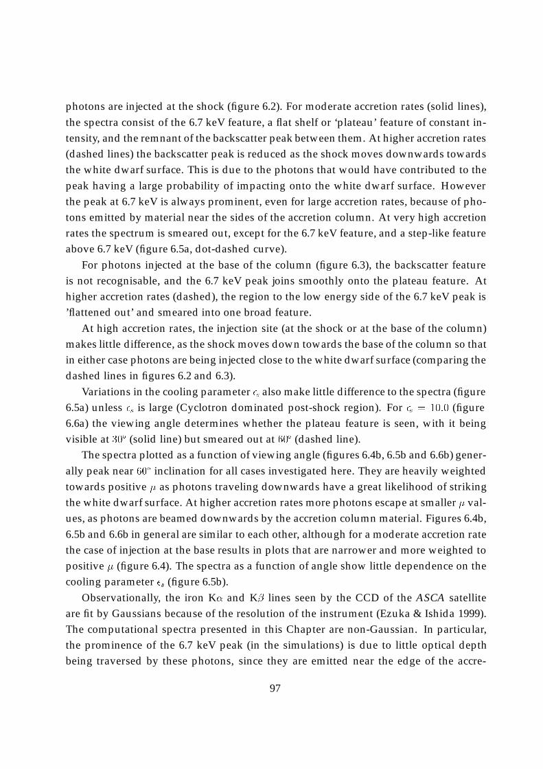
photons are injected at the shock (figure 6.2). For moderate accretion rates (solid lines),the spectra consist of the 6.7 keV feature, a flat shelf or ‘plateau’ feature of constant in-tensity, and the remnant of the backscatter peak between them. At higher accretion rates(dashed lines) the backscatter peak is reduced as the shock moves downwards towardsthe white dwarf surface. This is due to the photons that would have contributed to thepeak having a large probability of impacting onto the white dwarf surface. Howeverthe peak at 6.7 keV is always prominent, even for large accretion rates, because of pho-tons emitted by material near the sides of the accretion column. At very high accretionrates the spectrum is smeared out, except for the 6.7 keV feature, and a step-like featureabove 6.7 keV (figure 6.5a, dot-dashed curve).

For photons injected at the base of the column (figure 6.3), the backscatter featureis not recognisable, and the 6.7 keV peak joins smoothly onto the plateau feature. Athigher accretion rates (dashed), the region to the low energy side of the 6.7 keV peak is’flattened out’ and smeared into one broad feature.

At high accretion rates, the injection site (at the shock or at the base of the column)makes little difference, as the shock moves down towards the base of the column so thatin either case photons are being injected close to the white dwarf surface (comparing thedashed lines in figures 6.2 and 6.3).

Variations in the cooling parameter �s also make little difference to the spectra (figure6.5a) unless �s is large (Cyclotron dominated post-shock region). For �s = 10:0 (figure6.6a) the viewing angle determines whether the plateau feature is seen, with it beingvisible at 30� (solid line) but smeared out at 60� (dashed line).

The spectra plotted as a function of viewing angle (figures 6.4b, 6.5b and 6.6b) gener-ally peak near 60� inclination for all cases investigated here. They are heavily weightedtowards positive � as photons traveling downwards have a great likelihood of strikingthe white dwarf surface. At higher accretion rates more photons escape at smaller � val-ues, as photons are beamed downwards by the accretion column material. Figures 6.4b,6.5b and 6.6b in general are similar to each other, although for a moderate accretion ratethe case of injection at the base results in plots that are narrower and more weighted topositive � (figure 6.4). The spectra as a function of angle show little dependence on thecooling parameter �s (figure 6.5b).

Observationally, the iron K� and K� lines seen by the CCD of the ASCA satelliteare fit by Gaussians because of the resolution of the instrument (Ezuka & Ishida 1999).The computational spectra presented in this Chapter are non-Gaussian. In particular,the prominence of the 6.7 keV peak (in the simulations) is due to little optical depthbeing traversed by these photons, since they are emitted near the edge of the accre-

97

tion column. An absence (observationally) of this non-Gaussian peak feature, if found,would suggests that a more realistic source function would be one that is located cen-trally within the column. A greater amount of optical depth would then be seen bythe photons, smearing the intensity distribution into a broader (Gaussian-like) feature.Additionally, a photon source (emissivity function) that is peaked towards the centre ofthe column might also suggest the presence of a radial temperature or density gradient,from the centre to the edge of the accretion column, in addition to the gradients alongthe length of the column (away from the white dwarf star) as studied here. The sourcefunction can be inferred from the scattered line structure if observed at high enough res-olution, for instance with the grating spectrographs on board the Chandra satellite andXMM-Newton.

In summary, at high accretion rates the computational spectra are similar to eachother for different inclination angles and injection heights. At moderate accretion rates,and at a given the inclination angle, it may be possible in principle to determine theinjection height of the photons, from the presence or absence of the backscatter peak.However, to test this conjecture in future work one should include realistic emissivityfunctions, so photons are injected at different heights above the surface (a straightfor-ward modification) and perhaps at different radii within the column. The code de-scribed here can also in principle treat the case of neutron star accretion, after a modifi-cation of the post-shock cooling law and the inclusion of light bending near the neutronstar.

6.2 2D: Accretion disk

6.2.1 Rotating torus

The hard X-ray spectra of accreting compact objects is often interpreted in terms ofComptonization of soft photons off relativistic electrons. In this traditional interpre-tation, the scattering plasma is assumed to be isotropic and have either a power law ora Maxwellian distribution. Comptonization in such a plasma has been studied inten-sively over a number of years, both by analytic means (Sunyaev & Titarchuk 1980) andby means of Monte Carlo simulation (Pozdnyakov, Sobol & Sunyaev 1983; Stern et al1995).

An alternative possibility is that the momentum of the electrons is not primarily dueto an isotropic distribution, but rather is due to directed bulk motion of the plasma, or

98

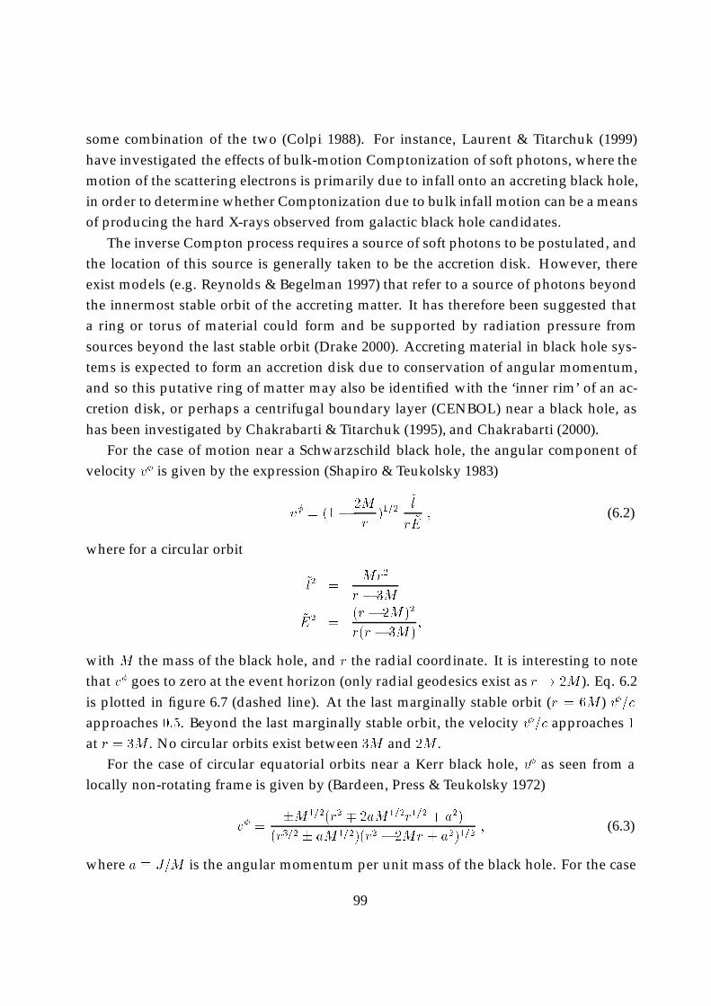
some combination of the two (Colpi 1988). For instance, Laurent & Titarchuk (1999)have investigated the effects of bulk-motion Comptonization of soft photons, where themotion of the scattering electrons is primarily due to infall onto an accreting black hole,in order to determine whether Comptonization due to bulk infall motion can be a meansof producing the hard X-rays observed from galactic black hole candidates.

The inverse Compton process requires a source of soft photons to be postulated, andthe location of this source is generally taken to be the accretion disk. However, thereexist models (e.g. Reynolds & Begelman 1997) that refer to a source of photons beyondthe innermost stable orbit of the accreting matter. It has therefore been suggested thata ring or torus of material could form and be supported by radiation pressure fromsources beyond the last stable orbit (Drake 2000). Accreting material in black hole sys-tems is expected to form an accretion disk due to conservation of angular momentum,and so this putative ring of matter may also be identified with the ‘inner rim’ of an ac-cretion disk, or perhaps a centrifugal boundary layer (CENBOL) near a black hole, ashas been investigated by Chakrabarti & Titarchuk (1995), and Chakrabarti (2000).

For the case of motion near a Schwarzschild black hole, the angular component ofvelocity v� is given by the expression (Shapiro & Teukolsky 1983)

v� = (1� 2M

r)1=2

~l

r ~E; (6.2)

where for a circular orbit

~l2 =Mr2

r � 3M

~E2 =(r � 2M)2

r(r � 3M);

with M the mass of the black hole, and r the radial coordinate. It is interesting to notethat v� goes to zero at the event horizon (only radial geodesics exist as r ! 2M ). Eq. 6.2is plotted in figure 6.7 (dashed line). At the last marginally stable orbit (r = 6M ) v�=capproaches 0:5. Beyond the last marginally stable orbit, the velocity v�=c approaches 1at r = 3M . No circular orbits exist between 3M and 2M .

For the case of circular equatorial orbits near a Kerr black hole, v� as seen from alocally non-rotating frame is given by (Bardeen, Press & Teukolsky 1972)

v� =�M1=2(r2 � 2aM1=2r1=2 + a2)

(r3=2 � aM1=2)(r2 � 2Mr + a2)1=2; (6.3)

where a � J=M is the angular momentum per unit mass of the black hole. For the case

99

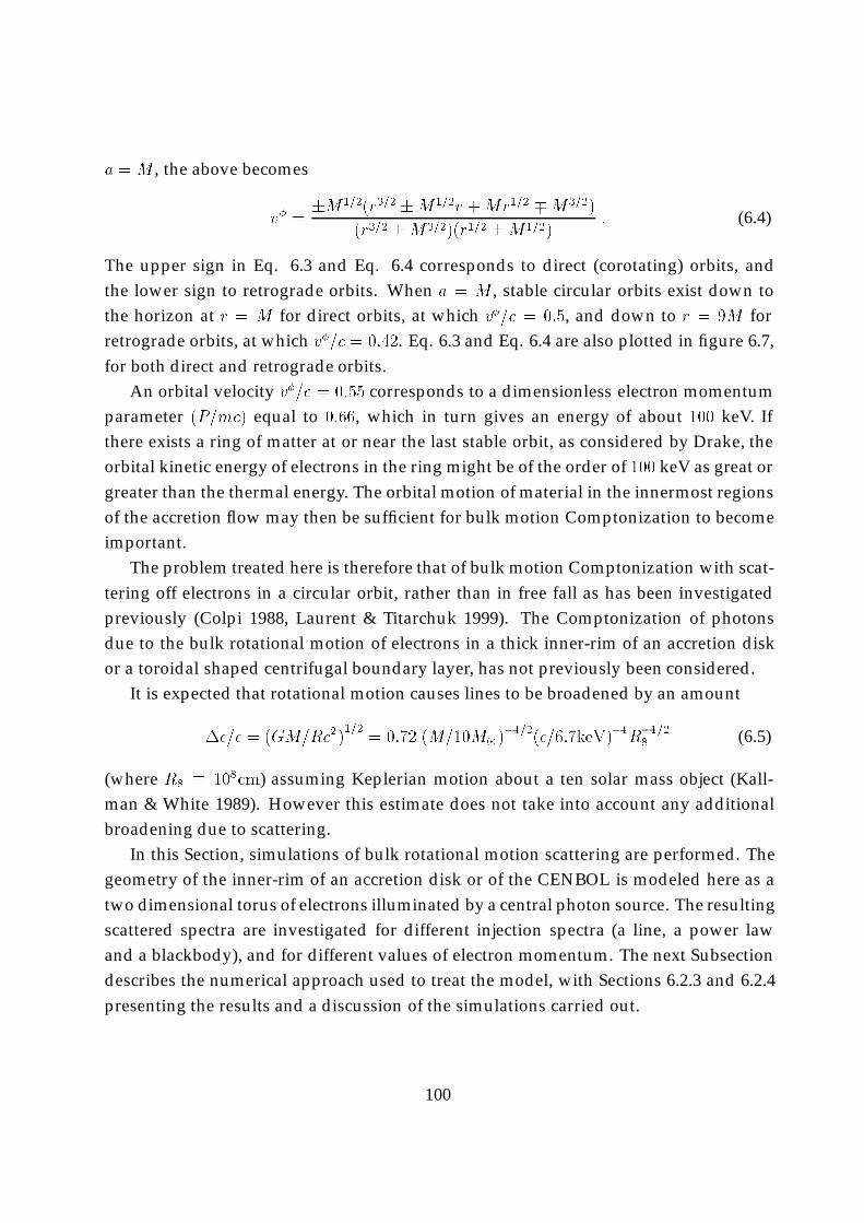
a = M , the above becomes

v� =�M1=2(r3=2 �M1=2r +Mr1=2 �M3=2)

(r3=2 �M3=2)(r1=2 �M1=2): (6.4)

The upper sign in Eq. 6.3 and Eq. 6.4 corresponds to direct (corotating) orbits, andthe lower sign to retrograde orbits. When a = M , stable circular orbits exist down tothe horizon at r = M for direct orbits, at which v�=c = 0:5, and down to r = 9M forretrograde orbits, at which v�=c = 0:42. Eq. 6.3 and Eq. 6.4 are also plotted in figure 6.7,for both direct and retrograde orbits.

An orbital velocity v�=c = 0:55 corresponds to a dimensionless electron momentumparameter (P=mc) equal to 0:66, which in turn gives an energy of about 100 keV. Ifthere exists a ring of matter at or near the last stable orbit, as considered by Drake, theorbital kinetic energy of electrons in the ring might be of the order of 100 keV as great orgreater than the thermal energy. The orbital motion of material in the innermost regionsof the accretion flow may then be sufficient for bulk motion Comptonization to becomeimportant.

The problem treated here is therefore that of bulk motion Comptonization with scat-tering off electrons in a circular orbit, rather than in free fall as has been investigatedpreviously (Colpi 1988, Laurent & Titarchuk 1999). The Comptonization of photonsdue to the bulk rotational motion of electrons in a thick inner-rim of an accretion diskor a toroidal shaped centrifugal boundary layer, has not previously been considered.

It is expected that rotational motion causes lines to be broadened by an amount

��=� = (GM=Rc2)1=2

= 0:72 (M=10M�)�1=2(�=6:7keV)�1R

�1=28 (6.5)

(where R8 � 108cm) assuming Keplerian motion about a ten solar mass object (Kall-man & White 1989). However this estimate does not take into account any additionalbroadening due to scattering.

In this Section, simulations of bulk rotational motion scattering are performed. Thegeometry of the inner-rim of an accretion disk or of the CENBOL is modeled here as atwo dimensional torus of electrons illuminated by a central photon source. The resultingscattered spectra are investigated for different injection spectra (a line, a power lawand a blackbody), and for different values of electron momentum. The next Subsectiondescribes the numerical approach used to treat the model, with Sections 6.2.3 and 6.2.4presenting the results and a discussion of the simulations carried out.

100

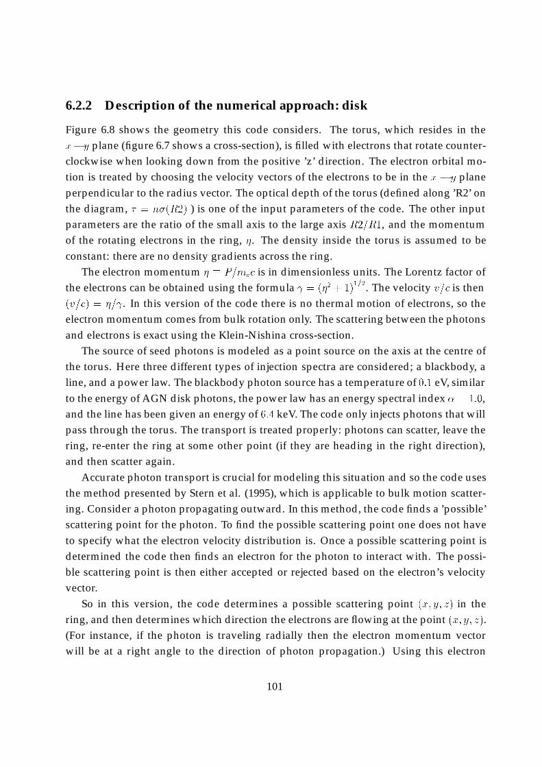
6.2.2 Description of the numerical approach: disk

Figure 6.8 shows the geometry this code considers. The torus, which resides in thex� y plane (figure 6.7 shows a cross-section), is filled with electrons that rotate counter-clockwise when looking down from the positive ’z’ direction. The electron orbital mo-tion is treated by choosing the velocity vectors of the electrons to be in the x � y planeperpendicular to the radius vector. The optical depth of the torus (defined along ’R2’ onthe diagram, � = n�(R2) ) is one of the input parameters of the code. The other inputparameters are the ratio of the small axis to the large axis R2=R1, and the momentumof the rotating electrons in the ring, �. The density inside the torus is assumed to beconstant: there are no density gradients across the ring.

The electron momentum � � P=mec is in dimensionless units. The Lorentz factor ofthe electrons can be obtained using the formula = (�2 + 1)

1=2. The velocity v=c is then(v=c) = �= . In this version of the code there is no thermal motion of electrons, so theelectron momentum comes from bulk rotation only. The scattering between the photonsand electrons is exact using the Klein-Nishina cross-section.

The source of seed photons is modeled as a point source on the axis at the centre ofthe torus. Here three different types of injection spectra are considered; a blackbody, aline, and a power law. The blackbody photon source has a temperature of 0:1 eV, similarto the energy of AGN disk photons, the power law has an energy spectral index � = 1:0,and the line has been given an energy of 6:4 keV. The code only injects photons that willpass through the torus. The transport is treated properly: photons can scatter, leave thering, re-enter the ring at some other point (if they are heading in the right direction),and then scatter again.

Accurate photon transport is crucial for modeling this situation and so the code usesthe method presented by Stern et al. (1995), which is applicable to bulk motion scatter-ing. Consider a photon propagating outward. In this method, the code finds a ’possible’scattering point for the photon. To find the possible scattering point one does not haveto specify what the electron velocity distribution is. Once a possible scattering point isdetermined the code then finds an electron for the photon to interact with. The possi-ble scattering point is then either accepted or rejected based on the electron’s velocityvector.

So in this version, the code determines a possible scattering point (x; y; z) in thering, and then determines which direction the electrons are flowing at the point (x; y; z).(For instance, if the photon is traveling radially then the electron momentum vectorwill be at a right angle to the direction of photon propagation.) Using this electron

101

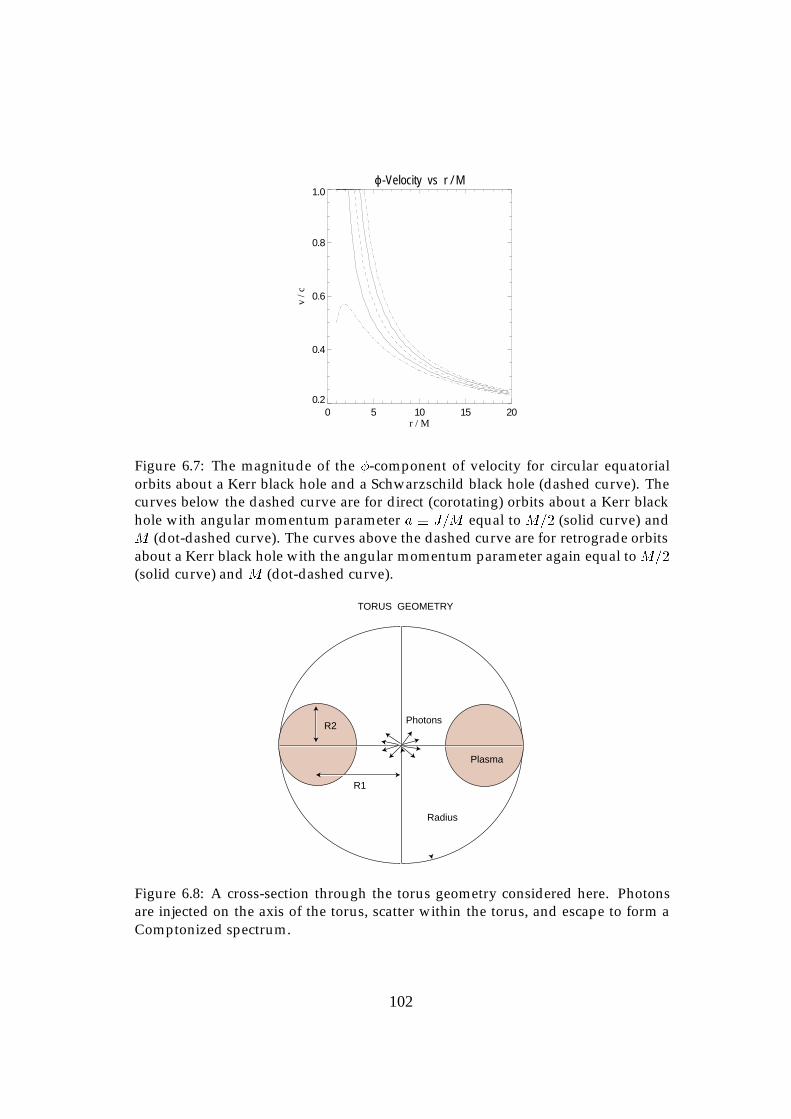
ϕ-Velocity vs r / M

0 5 10 15 20r / M

0.2

0.4

0.6

0.8

1.0

v / c

Figure 6.7: The magnitude of the �-component of velocity for circular equatorialorbits about a Kerr black hole and a Schwarzschild black hole (dashed curve). Thecurves below the dashed curve are for direct (corotating) orbits about a Kerr blackhole with angular momentum parameter a � J=M equal to M=2 (solid curve) andM (dot-dashed curve). The curves above the dashed curve are for retrograde orbitsabout a Kerr black hole with the angular momentum parameter again equal to M=2(solid curve) and M (dot-dashed curve).

R2

R1

TORUS GEOMETRY

Radius

Photons

Plasma

Figure 6.8: A cross-section through the torus geometry considered here. Photonsare injected on the axis of the torus, scatter within the torus, and escape to form aComptonized spectrum.

102

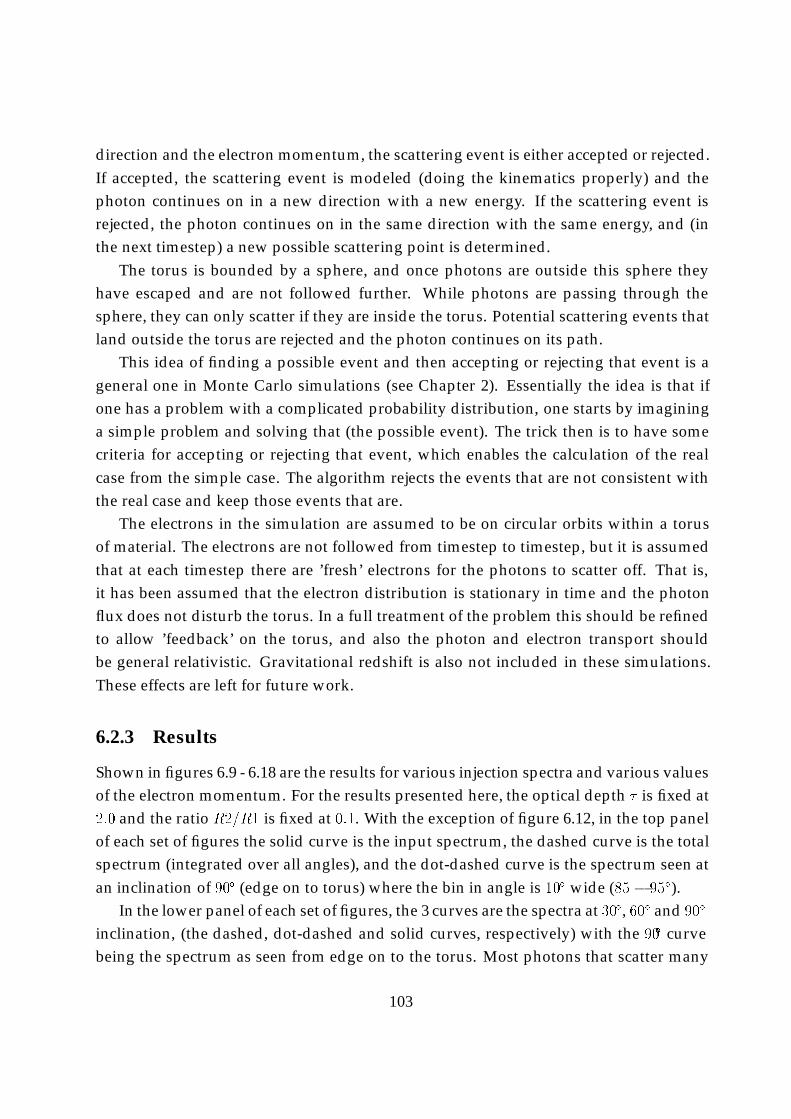
direction and the electron momentum, the scattering event is either accepted or rejected.If accepted, the scattering event is modeled (doing the kinematics properly) and thephoton continues on in a new direction with a new energy. If the scattering event isrejected, the photon continues on in the same direction with the same energy, and (inthe next timestep) a new possible scattering point is determined.

The torus is bounded by a sphere, and once photons are outside this sphere theyhave escaped and are not followed further. While photons are passing through thesphere, they can only scatter if they are inside the torus. Potential scattering events thatland outside the torus are rejected and the photon continues on its path.

This idea of finding a possible event and then accepting or rejecting that event is ageneral one in Monte Carlo simulations (see Chapter 2). Essentially the idea is that ifone has a problem with a complicated probability distribution, one starts by imagininga simple problem and solving that (the possible event). The trick then is to have somecriteria for accepting or rejecting that event, which enables the calculation of the realcase from the simple case. The algorithm rejects the events that are not consistent withthe real case and keep those events that are.

The electrons in the simulation are assumed to be on circular orbits within a torusof material. The electrons are not followed from timestep to timestep, but it is assumedthat at each timestep there are ’fresh’ electrons for the photons to scatter off. That is,it has been assumed that the electron distribution is stationary in time and the photonflux does not disturb the torus. In a full treatment of the problem this should be refinedto allow ’feedback’ on the torus, and also the photon and electron transport shouldbe general relativistic. Gravitational redshift is also not included in these simulations.These effects are left for future work.

6.2.3 Results

Shown in figures 6.9 - 6.18 are the results for various injection spectra and various valuesof the electron momentum. For the results presented here, the optical depth � is fixed at2:0 and the ratio R2=R1 is fixed at 0:1. With the exception of figure 6.12, in the top panelof each set of figures the solid curve is the input spectrum, the dashed curve is the totalspectrum (integrated over all angles), and the dot-dashed curve is the spectrum seen atan inclination of 90� (edge on to torus) where the bin in angle is 10� wide (85 � 95�).

In the lower panel of each set of figures, the 3 curves are the spectra at 30�, 60� and 90�

inclination, (the dashed, dot-dashed and solid curves, respectively) with the 90� curvebeing the spectrum as seen from edge on to the torus. Most photons that scatter many

103

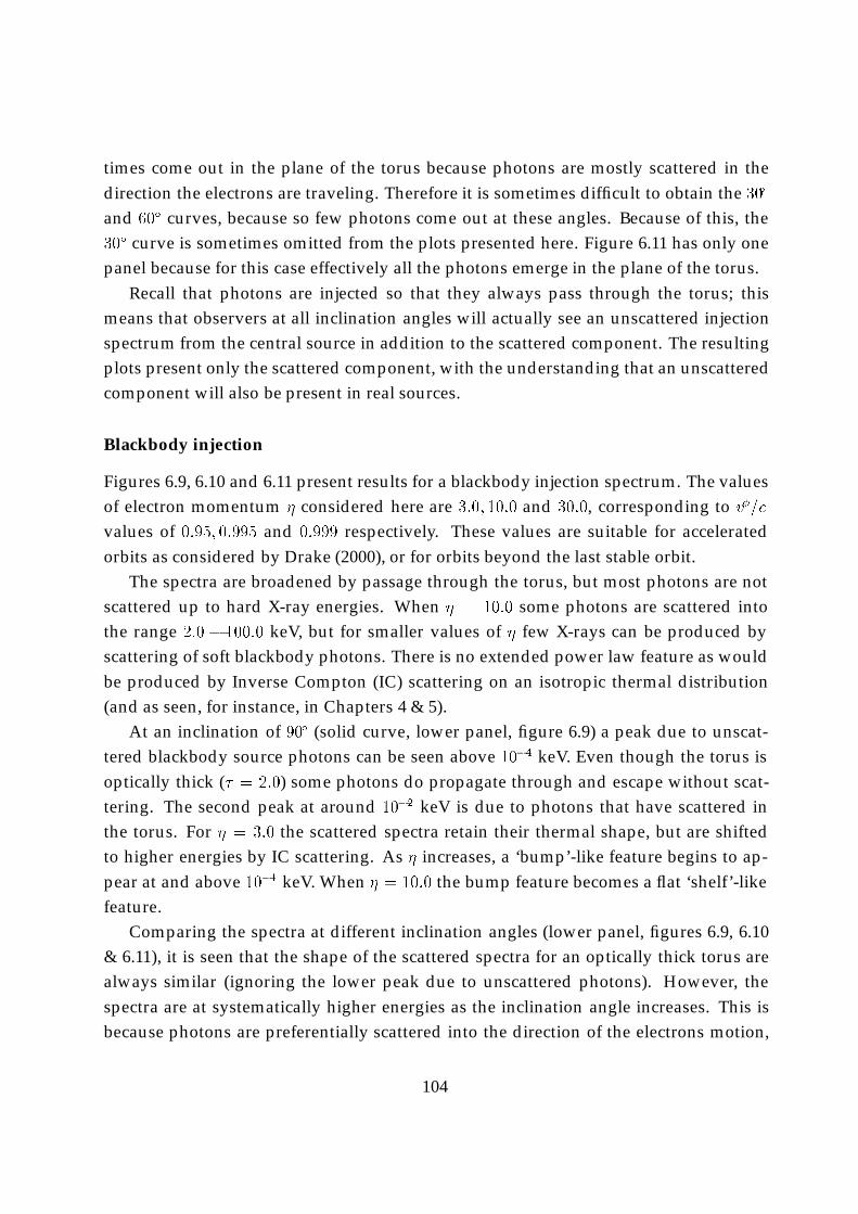
times come out in the plane of the torus because photons are mostly scattered in thedirection the electrons are traveling. Therefore it is sometimes difficult to obtain the 30�

and 60� curves, because so few photons come out at these angles. Because of this, the30� curve is sometimes omitted from the plots presented here. Figure 6.11 has only onepanel because for this case effectively all the photons emerge in the plane of the torus.

Recall that photons are injected so that they always pass through the torus; thismeans that observers at all inclination angles will actually see an unscattered injectionspectrum from the central source in addition to the scattered component. The resultingplots present only the scattered component, with the understanding that an unscatteredcomponent will also be present in real sources.

Blackbody injection

Figures 6.9, 6.10 and 6.11 present results for a blackbody injection spectrum. The valuesof electron momentum � considered here are 3:0; 10:0 and 30:0, corresponding to v�=c

values of 0:95; 0:995 and 0:999 respectively. These values are suitable for acceleratedorbits as considered by Drake (2000), or for orbits beyond the last stable orbit.

The spectra are broadened by passage through the torus, but most photons are notscattered up to hard X-ray energies. When � = 10:0 some photons are scattered intothe range 2:0� 100:0 keV, but for smaller values of � few X-rays can be produced byscattering of soft blackbody photons. There is no extended power law feature as wouldbe produced by Inverse Compton (IC) scattering on an isotropic thermal distribution(and as seen, for instance, in Chapters 4 & 5).

At an inclination of 90� (solid curve, lower panel, figure 6.9) a peak due to unscat-tered blackbody source photons can be seen above 10�4 keV. Even though the torus isoptically thick (� = 2:0) some photons do propagate through and escape without scat-tering. The second peak at around 10�2 keV is due to photons that have scattered inthe torus. For � = 3:0 the scattered spectra retain their thermal shape, but are shiftedto higher energies by IC scattering. As � increases, a ‘bump’-like feature begins to ap-pear at and above 10�1 keV. When � = 10:0 the bump feature becomes a flat ‘shelf’-likefeature.

Comparing the spectra at different inclination angles (lower panel, figures 6.9, 6.10& 6.11), it is seen that the shape of the scattered spectra for an optically thick torus arealways similar (ignoring the lower peak due to unscattered photons). However, thespectra are at systematically higher energies as the inclination angle increases. This isbecause photons are preferentially scattered into the direction of the electrons motion,

104

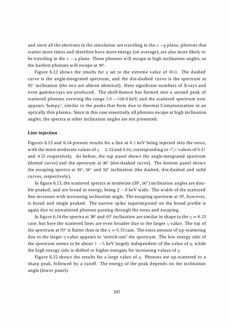
and since all the electrons in the simulation are traveling in the x�y plane, photons thatscatter more times and therefore have more energy (on average), are also more likely tobe traveling in the x� y plane. These photons will escape at high inclination angles, sothe hardest photons will escape at 90�.

Figure 6.12 shows the results for � set to the extreme value of 30:0. The dashedcurve is the angle-integrated spectrum, and the dot-dashed curve is the spectrum at90� inclination (the two are almost identical). Here significant numbers of X-rays andeven gamma-rays are produced. The shelf-feature has formed into a second peak ofscattered photons covering the range 2:0 � 100:0 keV, and the scattered spectrum nowappears ‘lumpy’, similar to the peaks that form due to thermal Comptonization in anoptically thin plasma. Since in this case essentially all photons escape at high inclinationangles, the spectra at other inclination angles are not presented.

Line injection

Figures 6.13 and 6.14 present results for a line at 6:4 keV being injected into the torus,with the more moderate values of � = 0:33 and 0:66, corresponding to v�=c values of 0:31and 0:55 respectively. As before, the top panel shows the angle-integrated spectrum(dotted curve) and the spectrum at 90� (dot-dashed curve). The bottom panel showsthe escaping spectra at 30�, 60� and 90� inclination (the dashed, dot-dashed and solidcurves, respectively).

In figure 6.13, the scattered spectra at moderate (30�, 60�) inclination angles are dou-ble peaked, and are broad in energy, being 2 � 3 keV wide. The width of the scatteredline increases with increasing inclination angle. The escaping spectrum at 90�, however,is broad and single peaked. The narrow spike superimposed on the broad profile isagain due to unscattered photons passing through the torus and escaping.

In figure 6.14 the spectra at 30� and 60� inclination are similar in shape to the � = 0:33

case, but here the scattered lines are even broader due to the larger � value. The top ofthe spectrum at 90� is flatter than in the � = 0:33 case. The extra amount of up-scatteringdue to the larger � value appears to ‘stretch-out’ the spectrum. The low energy side ofthe spectrum seems to be about 4 � 5 keV largely independent of the value of �, whilethe high energy side is shifted to higher energies for increasing values of �.

Figure 6.15 shows the results for a large value of �. Photons are up-scattered to asharp peak, followed by a cutoff. The energy of the peak depends on the inclinationangle (lower panel).

105

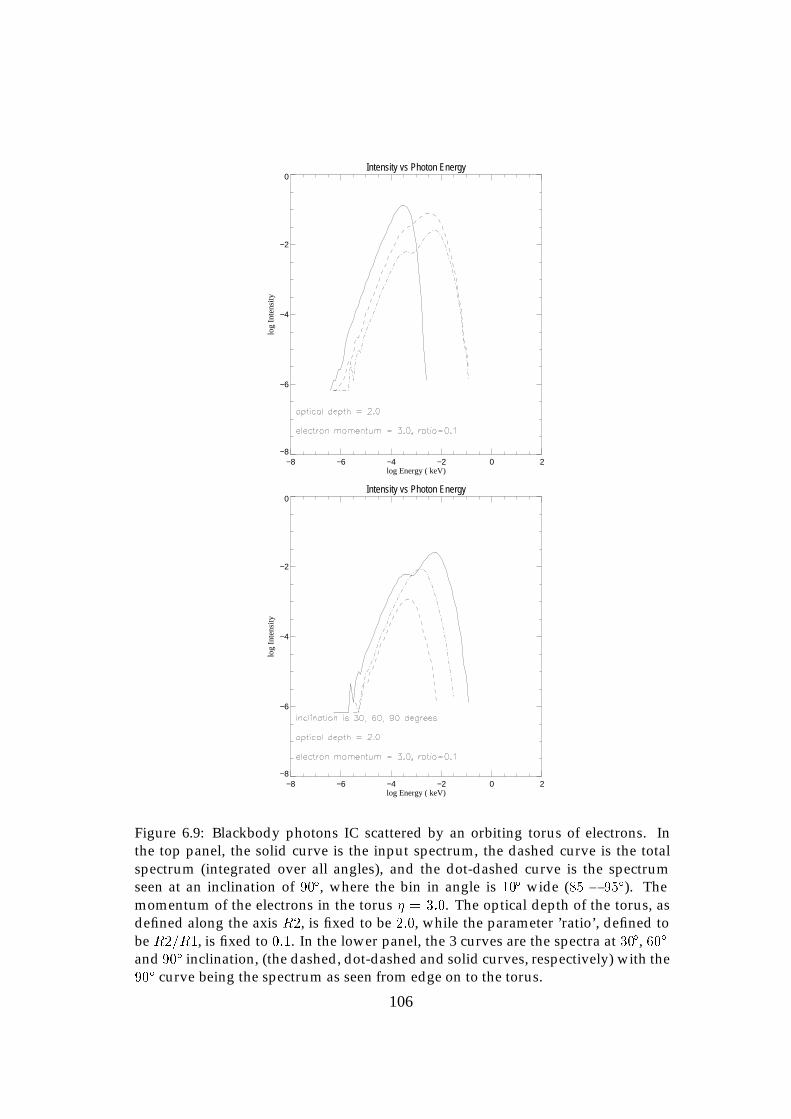
Intensity vs Photon Energy

−8 −6 −4 −2 0 2log Energy ( keV)

−8

−6

−4

−2

0

log

Inte

nsity

Intensity vs Photon Energy

−8 −6 −4 −2 0 2log Energy ( keV)

−8

−6

−4

−2

0

log

Inte

nsity

Figure 6.9: Blackbody photons IC scattered by an orbiting torus of electrons. Inthe top panel, the solid curve is the input spectrum, the dashed curve is the totalspectrum (integrated over all angles), and the dot-dashed curve is the spectrumseen at an inclination of 90�, where the bin in angle is 10� wide (85 � 95�). Themomentum of the electrons in the torus � = 3:0. The optical depth of the torus, asdefined along the axis R2, is fixed to be 2:0, while the parameter ’ratio’, defined tobe R2=R1, is fixed to 0:1. In the lower panel, the 3 curves are the spectra at 30�, 60�

and 90� inclination, (the dashed, dot-dashed and solid curves, respectively) with the90� curve being the spectrum as seen from edge on to the torus.

106

Intensity vs Photon Energy

−8 −6 −4 −2 0 2log Energy ( keV)

−8

−6

−4

−2

0

log

Inte

nsity

Intensity vs Photon Energy

−8 −6 −4 −2 0 2log Energy ( keV)

−8

−6

−4

−2

0

log

Inte

nsity

Figure 6.10: Blackbody photons IC scattered by an orbiting torus of electrons. Inthe top panel, the solid curve is the input spectrum, the dashed curve is the totalspectrum (integrated over all angles), and the dot-dashed curve is the spectrum seenat an inclination of 90�. The momentum of the electrons in the torus � = 6:0. In thelower panel, the 3 curves are the spectra at 30�, 60� and 90� inclination, (the dashed,dot-dashed and solid curves, respectively) with the 90� curve being the spectrum asseen from edge on to the torus.

107

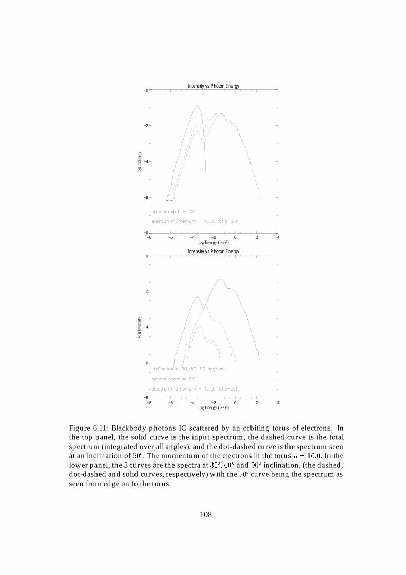
Intensity vs Photon Energy

−8 −6 −4 −2 0 2 4log Energy ( keV)

−8

−6

−4

−2

0

log

Inte

nsity

Intensity vs Photon Energy

−8 −6 −4 −2 0 2 4log Energy ( keV)

−8

−6

−4

−2

0

log

Inte

nsity

Figure 6.11: Blackbody photons IC scattered by an orbiting torus of electrons. Inthe top panel, the solid curve is the input spectrum, the dashed curve is the totalspectrum (integrated over all angles), and the dot-dashed curve is the spectrum seenat an inclination of 90�. The momentum of the electrons in the torus � = 10:0. In thelower panel, the 3 curves are the spectra at 30�, 60� and 90� inclination, (the dashed,dot-dashed and solid curves, respectively) with the 90� curve being the spectrum asseen from edge on to the torus.

108

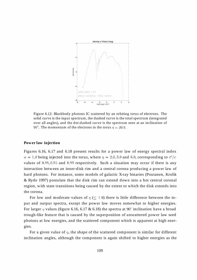
Intensity vs Photon Energy

−8 −6 −4 −2 0 2 4 6log Energy ( keV)

−8

−6

−4

−2

0

log

Inte

nsity

Figure 6.12: Blackbody photons IC scattered by an orbiting torus of electrons. Thesolid curve is the input spectrum, the dashed curve is the total spectrum (integratedover all angles), and the dot-dashed curve is the spectrum seen at an inclination of90�. The momentum of the electrons in the torus � = 30:0.

Power law injection

Figures 6.16, 6.17 and 6.18 present results for a power law of energy spectral index� = 1:0 being injected into the torus, where � = 2:0; 3:0 and 6:0, corresponding to v�=c

values of 0:89; 0:95 and 0:99 respectively. Such a situation may occur if there is anyinteraction between an inner-disk rim and a central corona producing a power law ofhard photons. For instance, some models of galactic X-ray binaries (Poutanen, Krolik& Ryde 1997) postulate that the disk rim can extend down into a hot central coronalregion, with state transitions being caused by the extent to which the disk extends intothe corona.

For low and moderate values of � (� 1:0) there is little difference between the in-put and output spectra, except the power law moves somewhat to higher energies.For larger � values (figure 6.16, 6.17 & 6.18) the spectra at 90� inclination have a broadtrough-like feature that is caused by the superposition of unscattered power law seedphotons at low energies, and the scattered component which is apparent at high ener-gies.

For a given value of �, the shape of the scattered component is similar for differentinclination angles, although the component is again shifted to higher energies as the

109

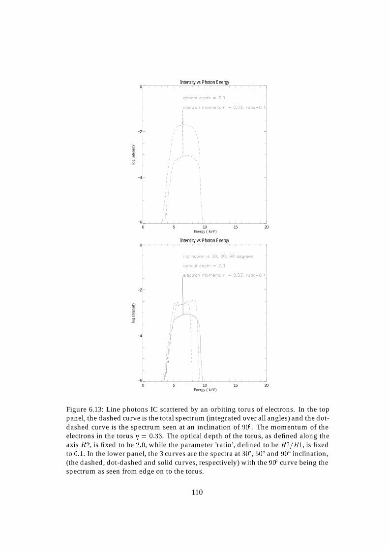
Intensity vs Photon Energy

0 5 10 15 20 Energy ( keV)

−6

−4

−2

0

log

Inte

nsity

Intensity vs Photon Energy

0 5 10 15 20 Energy ( keV)

−6

−4

−2

0

log

Inte

nsity

Figure 6.13: Line photons IC scattered by an orbiting torus of electrons. In the toppanel, the dashed curve is the total spectrum (integrated over all angles) and the dot-dashed curve is the spectrum seen at an inclination of 90�. The momentum of theelectrons in the torus � = 0:33. The optical depth of the torus, as defined along theaxis R2, is fixed to be 2:0, while the parameter ’ratio’, defined to be R2=R1, is fixedto 0:1. In the lower panel, the 3 curves are the spectra at 30�, 60� and 90� inclination,(the dashed, dot-dashed and solid curves, respectively) with the 90� curve being thespectrum as seen from edge on to the torus.

110

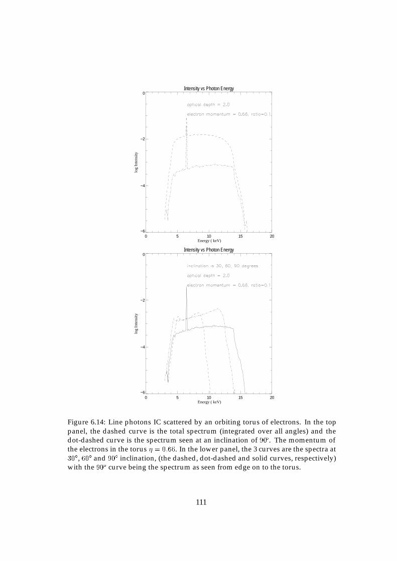
Intensity vs Photon Energy

0 5 10 15 20 Energy ( keV)

−6

−4

−2

0

log

Inte

nsity

Intensity vs Photon Energy

0 5 10 15 20 Energy ( keV)

−6

−4

−2

0

log

Inte

nsity

Figure 6.14: Line photons IC scattered by an orbiting torus of electrons. In the toppanel, the dashed curve is the total spectrum (integrated over all angles) and thedot-dashed curve is the spectrum seen at an inclination of 90�. The momentum ofthe electrons in the torus � = 0:66. In the lower panel, the 3 curves are the spectra at30�, 60� and 90� inclination, (the dashed, dot-dashed and solid curves, respectively)with the 90� curve being the spectrum as seen from edge on to the torus.

111

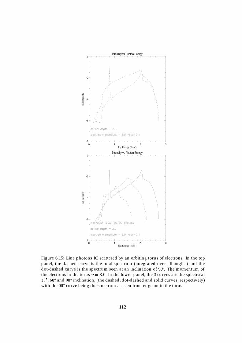
Intensity vs Photon Energy

0 1 2 3log Energy ( keV)

−8

−6

−4

−2

0

log

Inte

nsity

Intensity vs Photon Energy

0 1 2 3log Energy ( keV)

−8

−6

−4

−2

0

log

Inte

nsity

Figure 6.15: Line photons IC scattered by an orbiting torus of electrons. In the toppanel, the dashed curve is the total spectrum (integrated over all angles) and thedot-dashed curve is the spectrum seen at an inclination of 90�. The momentum ofthe electrons in the torus � = 3:0. In the lower panel, the 3 curves are the spectra at30�, 60� and 90� inclination, (the dashed, dot-dashed and solid curves, respectively)with the 90� curve being the spectrum as seen from edge on to the torus.

112

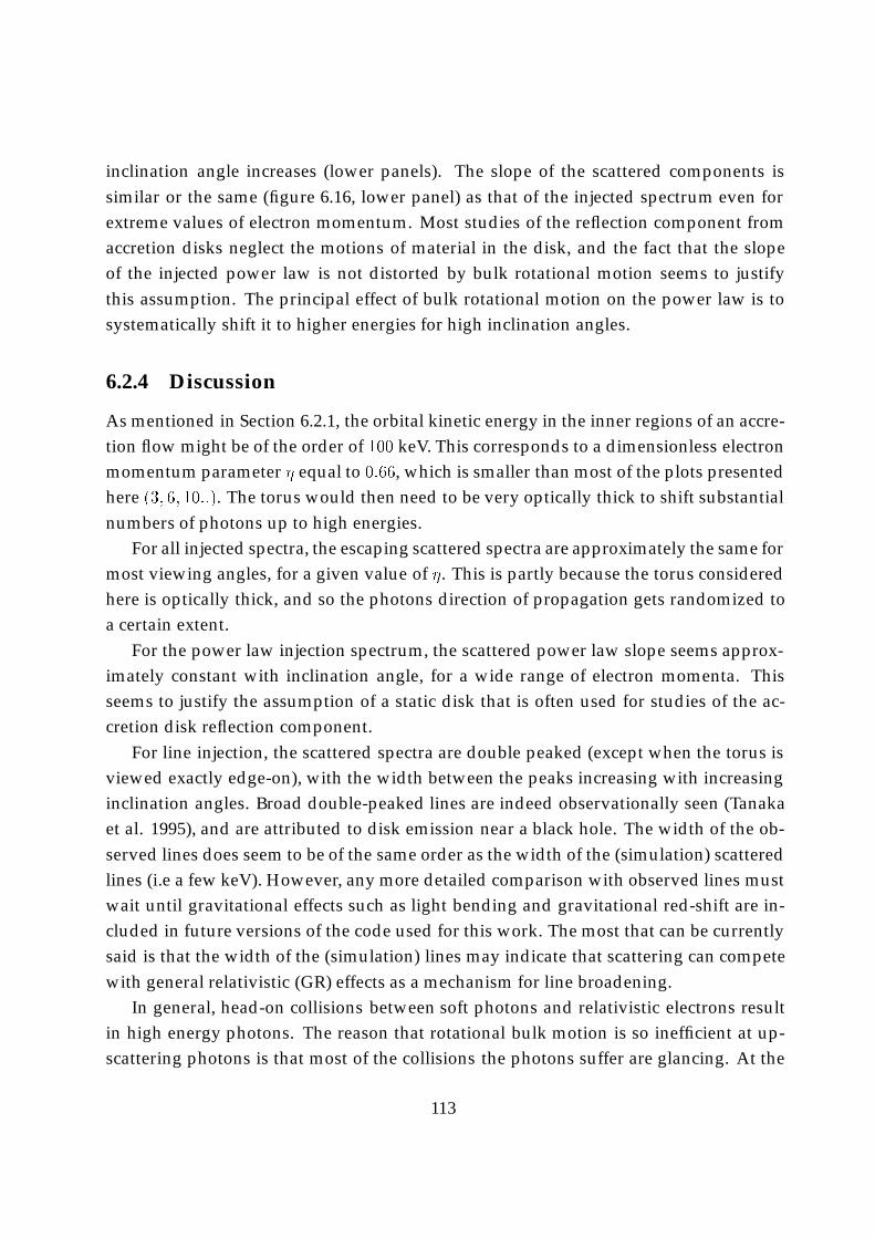
inclination angle increases (lower panels). The slope of the scattered components issimilar or the same (figure 6.16, lower panel) as that of the injected spectrum even forextreme values of electron momentum. Most studies of the reflection component fromaccretion disks neglect the motions of material in the disk, and the fact that the slopeof the injected power law is not distorted by bulk rotational motion seems to justifythis assumption. The principal effect of bulk rotational motion on the power law is tosystematically shift it to higher energies for high inclination angles.

6.2.4 Discussion

As mentioned in Section 6.2.1, the orbital kinetic energy in the inner regions of an accre-tion flow might be of the order of 100 keV. This corresponds to a dimensionless electronmomentum parameter � equal to 0:66, which is smaller than most of the plots presentedhere (3; 6; 10::). The torus would then need to be very optically thick to shift substantialnumbers of photons up to high energies.

For all injected spectra, the escaping scattered spectra are approximately the same formost viewing angles, for a given value of �. This is partly because the torus consideredhere is optically thick, and so the photons direction of propagation gets randomized toa certain extent.

For the power law injection spectrum, the scattered power law slope seems approx-imately constant with inclination angle, for a wide range of electron momenta. Thisseems to justify the assumption of a static disk that is often used for studies of the ac-cretion disk reflection component.

For line injection, the scattered spectra are double peaked (except when the torus isviewed exactly edge-on), with the width between the peaks increasing with increasinginclination angles. Broad double-peaked lines are indeed observationally seen (Tanakaet al. 1995), and are attributed to disk emission near a black hole. The width of the ob-served lines does seem to be of the same order as the width of the (simulation) scatteredlines (i.e a few keV). However, any more detailed comparison with observed lines mustwait until gravitational effects such as light bending and gravitational red-shift are in-cluded in future versions of the code used for this work. The most that can be currentlysaid is that the width of the (simulation) lines may indicate that scattering can competewith general relativistic (GR) effects as a mechanism for line broadening.

In general, head-on collisions between soft photons and relativistic electrons resultin high energy photons. The reason that rotational bulk motion is so inefficient at up-scattering photons is that most of the collisions the photons suffer are glancing. At the

113

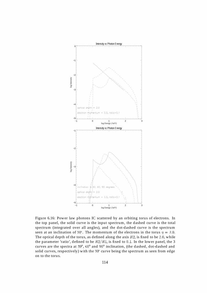
Intensity vs Photon Energy

−1 0 1 2 3log Energy ( keV)

−5

−4

−3

−2

−1

0

log

Inte

nsity

Intensity vs Photon Energy

−1 0 1 2 3log Energy ( keV)

−5

−4

−3

−2

−1

log

Inte

nsity

Figure 6.16: Power law photons IC scattered by an orbiting torus of electrons. Inthe top panel, the solid curve is the input spectrum, the dashed curve is the totalspectrum (integrated over all angles), and the dot-dashed curve is the spectrumseen at an inclination of 90�. The momentum of the electrons in the torus � = 2:0.The optical depth of the torus, as defined along the axis R2, is fixed to be 2:0, whilethe parameter ’ratio’, defined to be R2=R1, is fixed to 0:1. In the lower panel, the 3curves are the spectra at 30�, 60� and 90� inclination, (the dashed, dot-dashed andsolid curves, respectively) with the 90� curve being the spectrum as seen from edgeon to the torus.

114

Intensity vs Photon Energy

−1 0 1 2 3 4log Energy ( keV)

−5

−4

−3

−2

−1

0

log

Inte

nsity

Intensity vs Photon Energy

−1 0 1 2 3 4log Energy ( keV)

−5

−4

−3

−2

−1

log

Inte

nsity

Figure 6.17: Power law photons IC scattered by an orbiting torus of electrons. Inthe top panel, the solid curve is the input spectrum, the dashed curve is the totalspectrum (integrated over all angles), and the dot-dashed curve is the spectrumseen at an inclination of 90�. The momentum of the electrons in the torus � = 3:0. Inthe lower panel, the 2 curves are the spectra at 60� and 90� inclination, (dot-dashedand solid curves, respectively) with the 90� curve being the spectrum as seen fromedge on to the torus.

115

Intensity vs Photon Energy

−1 0 1 2 3 4log Energy ( keV)

−5

−4

−3

−2

−1

0

log

Inte

nsity

Intensity vs Photon Energy

−1 0 1 2 3 4log Energy ( keV)

−5

−4

−3

−2

−1

log

Inte

nsity

Figure 6.18: Power law photons IC scattered by an orbiting torus of electrons. Inthe top panel, the solid curve is the input spectrum, the dashed curve is the totalspectrum (integrated over all angles), and the dot-dashed curve is the spectrumseen at an inclination of 90�. The momentum of the electrons in the torus � = 6:0. Inthe lower panel, the 2 curves are the spectra at 60� and 90� inclination, (dot-dashedand solid curves, respectively) with the 90� curve being the spectrum as seen fromedge on to the torus.

116

first scattering event the angle between an electron and a photon is 90�, because thephotons are travelling radially. The photon will most probably be scattered into thedirection the electron is travelling, and so for any subsequent collisions the photon andelectron will be travelling in approximately the same direction. Head-on collisions arerare.

In summary, it seems that bulk rotational motion is an inefficient means of producinghard photons. Injected blackbody spectra form a peak at approximately the energy ofthe torus electrons. Injected power law spectra keep the same power law slope, but areshifted to higher energies. Therefore, the effect of bulk rotational scattering for thesetwo cases seems rather minimal. However, with reasonable parameters it is possibleto produce broad double-peaked lines (� a few keV wide). Scattering may thereforecompete with GR effects as a mechanism for line broadening.

6.3 Conclusion

The Monte Carlo numerical technique has been applied in this Chapter to astrophysicalproblems where bulk motion is important. In particular, simulations have been per-formed where density, temperature and bulk motion with velocity gradients are presentin the problem (the white dwarf case). It has been seen that the spectra are alwayspeaked near the injection energy, and often single peaked due to the second peak be-ing diminished as the shock approaches the white dwarf surface. A further applicationis to rotational motion Compton scattering, which should be a fundamental process ifphotons encounter electrons in orbit about a compact object. With moderate values ofelectron momentum, it is found that lines can be significantly broadened by rotationalCompton scattering.

117

References

Aizu, K. 1973, Prog. Theor. Phys., 49, 1184Bardeen, J. M., Press, W. H. & Teukolsky, S. A. 1972, ApJ, 178, 347Chakrabarti, S. K. 2000, Class. Quan. Grav., v17, 12, 2427 (arXiv:astro-ph/0007259)Chakrabarti, S. K. & Titarchuk, L. 1995, ApJ, 455, 623Colpi, M. 1988, ApJ, 326, 223Drake, S. P. 2000, in press (arXiv:gr-qc/0010082)Ezuka, H. & Ishida, M. 1999, ApJ Supplement 120, 277Frank, J., King, A. R. & Raine, D. J. 1985, ”Accretion Power in Astrophysics”, (Cam-

bridge University Press)Fujimoto, R. & Ishida, M. 1997, ApJ, 474, 774Hua, X. 1997, Comp. Ph., 11, 660 (see also arXiv:physics/9709023)Ishida. M., et al. 1994, MNRAS, 266, 367Ishida, M., Mukai, K. & Osborne, J. P. 1994, PASJ, 46, L81Kallman, T. & White, N. E. 1989, ApJ, 341, 955Laurent, P. & Titarchuk, T. 1999 ApJ, 511, 289Poutanen, J. Krolik, J. & Ryde, F. 1997, MNRAS, 292, L21Pozdnyakov, L. A., Sobol, I. M. & Sunyaev, R. A. 1983, Ap.& Space Sci. Reviews, 2, 189Reynolds, C. S. & Begelman, M. C. 1997, ApJ, 488, 109Shapiro, S. L. & Teukolsky, S. A. 1983, ”Black Holes, White Dwarfs and Neutron Stars,

The Physics of Compact Objects”, (John Wiley & Sons)Stern, B., et al. 1995, MNRAS, 272, 291Sunyaev, R. A. & Titarchuk, L. 1980, A&A, 86, 121Tanaka, Y. et al. 1995, Nature, 375, 659Wu, K., Chanmugan, G., & Shaviv, G. 1994, ApJ, 426, 664

118

Chapter 7

Conclusions

Analytic results

This thesis has studied the Inverse Compton scattering mechanism in astrophysics, pri-marily via numerical studies. Chapter 1 reviewed the fundamental analytic results re-quired for the interpretation of Comptonized spectra, results that were derived for thecase of large optical depth when an approach based on the diffusion equation is suitable.Further, Chapter 1 presented a short introduction to the astrophysical systems withinwhich Compton scattering is thought to be important for spectral formation. The rea-son that feedback is considered an important ingredient for disk-corona models wasalso discussed, using the expression for the spectral index.

Semi-analytic disk-corona models with feedback were considered in detail in Chap-ter 4, with the effect of a disk wind or outflow on the energy balance of the disk, andtherefore on the X-ray spectrum, being considered. While the presence of a wind canresult in a hotter corona and harder X-ray spectra, the wind parameter must be large forthis to occur. Only then can significant power be extracted from the disk to reduce thephoton flux cooling the corona. It was also seen that a situation is possible where in-creasing the optical depth of the corona results in a harder X-ray spectrum, the oppositeto the trend usually considered.

Numerical advance

Since numerical approaches based on the Monte Carlo technique are generally consid-ered the most flexible, Chapter 2 provided both an introduction to the Monte Carlotechnique and the application of this technique to the specific case of inverse Comptonscattering. The method of modeling a scattering event via the differential cross-section

119

and the method of transporting photons from one scattering event to the next were pre-sented.

The photon transport method becomes more difficult if the situation to be studiedinvolves an electron distribution that is not isotropic. An elegant algorithm for treat-ing these situations is the non-linear Monte Carlo approach. Chapter 3 discussed this,and then proposed and implemented an extension to this algorithm that enables thestraightforward calculation of scattering in situations where the electron distribution isa complicated function of position. It was seen that such an algorithm is suitable forthe calculation of scattering in plasmas containing bulk flow of electrons in addition totemperature and density gradients.

Applications of the numerical approach

The linear Monte Carlo approach was applied in Chapter 5 to a study of the time lagsthat are to be expected in the X-ray light curves of Cyg X-1 due to the Comptonizationof photons in a corona that may consist of a multi-temperature plasma. It was shownthat the phase and time lag curves contain a rise at low Fourier frequencies indicatingthe presence of an outer corona of plasma. The temperature of this outer corona did notgreatly affect the time lags, however its optical depth did effect the time lags as more orfewer scattering events took place in the outer corona.

The flexible numerical method presented in Chapter 3 has some immediate applica-tions; namely to photon scattering in situations where bulk motion as well as temper-ature variations are important. Such a situation is the case of photon scattering in anaccretion column. Chapter 6 presented a numerical study of this situation and it wasfound that variations in the cooling parameter of the post-shock region made little dif-ference to the scattered spectrum. At high accretion rates, the second or ’backscatter’peak is attenuated as those photons are beamed downward by the accretion flow andhave a high probability of impacting the white dwarf surface. The spectra as a functionof viewing angle also are little affected by the value of the post-shock cooling parameter.At moderate accretion rates the strength of the backscatter peak could be a guide to thelocation of the photon source (at the shock or at the base of the column).

A basic process that has until now not been considered is electron-photon scatteringwhen the electron’s momentum is due to orbital motion; a situation termed bulk rota-tional scattering. This process was also studied in Chapter 6 for a toroidal geometry and,in a key conclusion of this work, bulk rotational scattering was found to significantlybroaden a line of photons when the orbital velocity of the electrons in the orbiting torus

120

was greater than about 0:3c. The effect on the energy distribution of injected blackbodyphotons was to produce a peak in the scattered distribution at the energy of the orbitingelectrons, while power law distributions of photons are little affected by scattering inthe torus.

In summary, the codes written using the algorithms in this thesis were successfully ap-plied to a number of astrophysical situations that had either not been studied previously(the bulk rotational scattering calculation), or had used approximate methods (the whitedwarf accretion column calculation). Monte Carlo techniques are now flexible enoughto treat most scattering problems of interest in astrophysics.

121

Part IV

Appendix

122

Appendix A

Monte Carlo photon transport code

program compton photons

cccccccccccccccccccccccccccccccccccccccccccccccccccccccccccccc cccccccccc This is a code that calculates Compton scatteringc in a weakly magnetised White Dwarf star accretion column.cc This Monte Carlo code calculates the spectrum producedc by inverse Compton scattering of photons off Maxwellanc electrons in a cylindrical geometry, with density and velocityc gradients in the column. The cylinder extends along the x-axis.cc The distance between events is determined using a modifiedc non-linear transport method. The full Klein-Nishinac cross-section is used.cc The actual scattering events are modelled according to thec Pozdnyakov, Sobol’ and Sunyaev method.cc Inputs are the mass and radius of the white dwarf star, thec specific accretion rate, the viewing (inclination) angle,c and the ratio of bremstrahlung to cyclotron cooling in thec post-shock region.cc The scattered spectrum output file is fort.12c The photon distribution with escape angle output file is fort.13ccccccccccccccccccccccccccccccccccccccccccccccccccccccccccccccccccccccccc

123

ccccccccccccccccccccccccccccccccccccccccccccccccccccccccccccccccccccccccc definitions of some variablescc wdmass mass of the white dwarf star (solar mass units)c wdradius radius of the white dwarf star (cm)c wdaccretion total accretion rate (grams per second)c e0, e1 energy of first/last energy bins in eV, linear scalec nbintotal total number of energy binsc nphot total number of photon trajectoriesc bin1 output spectrum binsc bin2 output pulse profile binsc dontbin ignores the photon if .true.c ebin1(k) energy of bin1(k) in eV, it is used to binc both the input & output spectra.c abin1(k) angular bins, used for pulse profilec genrand() name of random number generator (not included in code)c nbin(k) number of photons in ebin1(k), input spectrumc pi constant pic amc2 constant electron rest energyc omfp mean free path (mfp)c aradius radius of accretion column, in units of Thompson mfpc tau Thompson optical depth in the accretion columnc done2 ends a photon trajectory when .true. (photon escape)c dcce distance to the white dwarf from photon positionc bbtemp plank temperature of source photons in units of eVc plank switch between plank (1.0) and line photon injectionc electemp maxwellian temperature of electrons in units of mc2

c vel(k) velocity profile of the post-shock regionc dens(k) density profile of the post-shock regionc temp(k) temperature profile of the post-shock regionc shockh height of the accretion shock above WD surfacec acolumn the total length of the accretion columnc aradiuswd dimentionless constant, related to white dwarf radiusc binlinear switch between linear and log energy bins.(0.0=log)c cyclotron ratio of cyclotron cooling to bremstrahlung coolingc in the post-shock regionc isotropic isotropic photon injection if equal to onec plank switch between blackbody and line injectionc aline input line energy in eVc ainclination the inclination angle that the system is seen fromc ainca/b how wide the inclination angle bin isc shocktemp the temperature of the accretion shock

124

c x1, x2, x3 the current location of the photon (vector)c omeg1, 2, 3 the current photon propagation direction (vector)ccccccccccccccccccccccccccccccccccccccccccccccccccccccccccccccccccccccccc

implicit real*8 (a-h, o-z)logical done, done2, dontbindimension nbin(1:10000)dimension bin1(1:100000)dimension bin2(1:100000)dimension ebin1(1:10000)dimension abin1(1:10)dimension vel(1:1001)dimension dens(1:1001)dimension temp(1:1001)

ccccccccccccccccccccccccccccccccccccccccccccccccccccccccccccccccccccccccc INPUT PARAMETERS OF THE SIMULATION, which have been taken fromc the paper by Wu, Chanmugam & Shaviv 1994, ApJ, 426, 664c with additional relations as listed in Fujimoto & Ishida 1997, ApJ, 474, 774cc mass of the white dwarf star (solar mass units)

wdmass=0.5c radius of the white dwarf star (cm)

wdradius=1.0e+09c specific accretion rate (grams per cm2 per second)

wdaccretion=60.0c ratio of cyclotron cooling to bremstrahlung cooling in the post-shock

cyclotron=10.0c the inclination angle the spectrum is seen from (degrees)

ainclination=30.0c electron free-fall velocity just above the shock (v/c)

velff=(0.0123)*((wdmass/0.5)**0.5)* ((wdradius/1.0e+9)**-0.5)c electron temperature at the shock, in units of 16 keV

shocktemp=(0.0313111)*(wdmass/0.5)* ((wdradius/1.0e+9)**-1.0)c non-magnetic shock height (cm)

shockheight=(7.59e+6)*((wdaccretion/4.0)**-1.0)*+ ((wdmass/0.5)**1.5)*((wdradius/1.0e+9)**-1.5)

c dimensionless radius of the accretion column (a constant)aradius=50.0

c dimensionless radius of the white dwarf star (a constant)aradiuswd=10.0*aradius

c the length of the accretion columnacolumn=aradiuswd + (aradiuswd/2.0)

c the optical depth of the accretion column just above the shock

125

tau=(((6.65e-25)*(aradius/aradiuswd)*(1.0e+9))+ /1.6726e-24)*(wdaccretion/(velff*3.0e+10))

c output energy limits in electron voltse0=6000.0e1=7000.0

c switch between linear and log bins.(1.0=linear)binlinear=1.0

c switch between line (0.0) or blackbody injection photons (1.0)plank=0.0

c input temperature of blackbody source photons, in electron voltsbbtemp=130.0

c input line energy (eV)aline=6700.0

c isotropic photon injection if equal to one (1.0)isotropic=1

c inject photons isotropically at the shock if equal to one (1.0)top=1.0

c this is the total number of energy bins for the spectrumnbintotal=100

c when a photon has escaped from the accretion column, thisc becomes .true. and we stop following the photon.

done2=.false.c the number of photons in the simulation

nphot=10000type *, ”number of photons? (integer)”accept *, nphot

c in addition, other constants that the code requires are...ccc=3.0e8pi=atan(1.0)*4.0pi2 = pi*2.0amc2=511.0e3idummy = (2**19)+1

c bin spectrum between these two anglesainca=cos((ainclination+5.0)*(pi/180.0))aincb=cos((ainclination-5.0)*(pi/180.0))

c or alternatively, bin the angle integrated spectrumc ainca=-1.0c aincb=1.0cccccccccccccccccccccccccccccccccccccccccccccccccccccccccccccccccccccccc

c BEGINNING OF THE CODE: MAIN

126

c determine the energy bins and the angular binscall start1(binlinear, nbintotal, e1, e0, ebin1, anglebin, abin1, pi)

c determine the post-shock density, temperature & velocity profilesc that the photons will propagate through.

call profiles(vel, dens, temp, shockh, aradiuswd, cyclotron,+ shockheight, wdradius)

c start a photon trajectorydo j = 1, nphot

c inject the photon into the accretion columncall start2(omeg1, omeg2, omeg3, isotropic, aline,

+ x1, x2, x3, ncount3, bbtemp, aradius, aradiuswd,+ omegnew1, omegnew2, omegnew3, dontbin, velff,+ energy, energy1, shockh, plank, top,+ pi, pi2, idummy, dist, dist1, dcce, done, done2)

scatcount=0.0

c and begin the photon trajectorydo while(.not.done2)

c (never needed, this is here as a failsafe only)call stop(ncount3, energy, j, done2, dontbin)

c find the next scattering point for the photoncall transport(aradius, aradiuswd, tau, shockh, acolumn, index,

+ dens, alambda, x1, x2, x3, omeg1, omeg2, omeg3)

c the new photon scattering point is..x1new=x1+alambda*omeg1x2new=x2+alambda*omeg2x3new=x3+alambda*omeg3

c has the photon escaped from the accretion column?call geometry(x1, x2, x3, x1new, x2new, x3new, alambda,

+ aradius, aradiuswd, acolumn, omeg1, omeg2, omeg3,+ dontbin, done2)

if (.not.done2) thenc if it has not escaped then...

127

c now we determine the velocity of the accretion flow at this pointcall frame1(gamma1, vpf, index,

+ x1new, velff, aradiuswd, shockh, vel)

c now model the actual scattering event.call scattering1(omeg1, omeg2, omeg3, cold,

+ x1new, x2new, x3new, ncount3sum, index,+ omegnew1, omegnew2, omegnew3, shocktemp,+ energy, electemp, idummy, temp, gamma1, vpf,+ done2, amc2, pi, pi2, j, scatcount)

c update photon locationx1=x1newx2=x2newx3=x3new

c update the photon directionomeg1=omegnew1omeg2=omegnew2omeg3=omegnew3

c energy is updated in the scattering subroutine.

endif

enddoc end of current photon trajectory!!

c sort into bins (input spectrum)call bin input(ebin1, energy1, nbin, ii, nbintotal)

c sort into bins (output spectrum)c if the photon has not been killed,

if (.not.dontbin) then

c scatcount is the scattering order, 1, 2, 3...c if (scatcount.eq.1.0) thenc and if the photon is at the correct inclination angle, bin it.

if (omeg1.ge.ainca) thenif (omeg1.le.aincb) thencall bin output(ebin1, energy, bin1, ii, nbintotal, j)

128

endifendif

c endif

c also, sort photons into angular bins (output spectrum)call bin profile(abin1, omeg1, bin2, ii, nbintotal)

endif

enddoc end of all photon trajectories, nphot!!

c output to files (bin1 is scattered spectrum)call output(ebin1, nbin, bin1, nbintotal, nphot, abin1,

+ bin2, ncount3sum, binlinear)

stopend

129

subroutine bin input(ebin1, energy1, nbin, ii, nbintotal)c This subroutine sorts the input photons drawn from ’blackbody’c into bins (input spectrum)

implicit real*8 (a-h, o-z)

dimension ebin1(1:10000)dimension nbin(1:10000)logical done

ii=1done = .false.

350 if (.not.done) then

if (ebin1(ii).ge.energy1) thendone = .true.nbin(ii)=nbin(ii)+1elseii=ii+1endifif (ii.gt.nbintotal) thenprint *, ”photon off scale”, j, ebin1(nbintotal), energy1stopendifgoto 350endif

returnend

130

subroutine bin output(ebin1, energy, bin1, ii, nbintotal, j)c This subroutine sorts the scattered photons into binsc (output spectrum)

implicit real*8 (a-h, o-z)

dimension ebin1(1:10000)dimension bin1(1:100000)logical done

ii=1done = .false.

400 continueif (done.eq..false.) then

if (ebin1(ii).ge.energy) thendone = .true.bin1(ii)=bin1(ii)+1.0

else

ii=ii+1endifif (ii.gt.nbintotal) thenbin1(nbintotal)=bin1(nbintotal)+1.0done = .true.endif

goto 400endif

returnend

131

subroutine bin profile(abin1, omeg1, bin2, ii, nbintotal)c This subroutine sorts the scattered photons into angular binsc pulse profile (output spectrum)

implicit real*8 (a-h, o-z)

dimension abin1(1:10)dimension bin2(1:100000)logical done

ii=1done = .false.

425 continueif (done.eq..false.) then

if (abin1(ii).le.omeg1) thendone = .true.bin2(ii)=bin2(ii)+1.0

else

ii=ii+1endifif (ii.gt.nbintotal) thenbin2(nbintotal)=bin2(nbintotal)+1.0done = .true.endif

goto 425endif

returnend

132

subroutine blackbody(idummy, energy, bbtemp)c This subroutine assigns an initial energy for each photonc that is drawn from a Plank blackbody.c variable ’energy’ is the photon energy.

implicit real*8 (a-h, o-z)

c energy/temp in units of eVtemp=bbtemp

eps5=1.0-genrand()eps6=1.0-genrand()eps7=1.0-genrand()eps8=1.0-genrand()

test3=1.202*eps5

if (test3.lt.1.0) thenalpha=1.0elseaa=1.0h=1.0do while (aa.le.test3)h=h+1.0aa=aa+(1.0/(h**3))enddo

alpha=hendif

energy=-1.0*(temp/alpha)*log(eps6*eps7*eps8)if ((energy.gt.1.0e30).or.(energy.le.0.0)) thenprint *, ”crazy input photons”endif

returnend

133

subroutine direction1(v1, v2, v3, brow, pi2)

c This returns a random electron incident directionc or a random initial photon direction.

implicit real*8 (a-h, o-z)

brow=0.0do while (brow .eq. 0.0)yyran=1.0-genrand()v3=2.0*genrand()-1.0vsq = sqrt(1.0-v3*v3)svv = sin(pi2*yyran)v2=vsq*svvv1=vsq*cos(pi2*yyran)brow=sqrt(v1*v1+v2*v2)enddo

returnend

134

subroutine frame1(gamma1, vpf, index,+ x1new, velff, aradiuswd, shockh, vel)

c this subroutine determines the velocity and gamma factor of thec flow at the potential scattering point. This is needed for thec Lorentz transform out of the flow rest frame.

implicit real*8 (a-h, o-z)dimension vel(1:1001)

c find the height of the photon above the white dwwarf, and thenc get the velocity of the flow at that point.

index=int(((x1new-aradiuswd)/(shockh))*1000.0)index=index+1if (index.le.0) thenindex=1endifif (index.le.1000) then

c if photon is in the post-shock region, then velocity isvpf=velff*vel(index)else

c if photon is in the pre-shock region, then velocity isvpf=velffendif

c Lorentz factor of accretion flowgamma1=1.0/(sqrt(1.0-vpf*vpf))

returnend

135

subroutine frame2(eta, gamma1, vpf, v1, v2, v3, brow)

c this subroutine Lorentz transforms out of the accretion flow restc frame, and back into the white dwarf frame.

implicit real*8 (a-h, o-z)

c Lorentz transform back into the White Dwarf rest frame.c ”eta” is now the new electron momentum in the new frame.c gamma1 and vpf are the lorentz factor and velocity at the pointc of the possible scattering event.

if (eta.eq.0.0) thenc then there is no thermal motion, and the electron is simply movingc with the flow.

eta=(gamma1)*(vpf)v1=-1.0v2=0.0v3=0.0brow=sqrt(v1*v1+v2*v2)else

c The electron momentum vector in the White Dwarf rest frame is ..ee1=v1*eta-eta*

+ (gamma1*vpf-(gamma1-1.0)*v1*(1.0))*(1.0)ee2=v2*etaee3=v3*eta

c convert to a unit vector plus a magnitudeamagnew=(ee1*ee1+ee2*ee2+ee3*ee3)**(0.5)

c the direction back in the ’lab’ frame (WD star at rest) is ..v1=ee1/amagnewv2=ee2/amagnewv3=ee3/amagnewbrow=sqrt(v1*v1+v2*v2)

c energy back in the ’lab’ WD frame is noweta=amagnew

endif

returnend

136

subroutine geometry(x1, x2, x3, x1new, x2new, x3new, alambda,+ aradius, aradiuswd, acolumn, omeg1, omeg2, omeg3,+ dontbin, done2)

c This subroutine keeps track of the photon as itc propagates through the geometry and determines if it isc outside the accretion column or if it has hit the Whitec Dwarf surface.

implicit real*8 (a-h, o-z)logical done2, dontbin

c photon distance from central axis of the accretion columndist=(x2new*x2new+x3new*x3new)**(1.0/2.0)

c if photon is outside the accretion column, stop the trajectory.if (dist.gt.aradius) thendone2=.true.endif

c if photon is outside the ’top’ of the accretion column, stop traj.if (x1new.gt.acolumn) thendone2=.true.endif

c check if photon will impact on the White Dwarf surface.c If so, kill the photon.

dcce=0.0dist1=(x1*x1+x2*x2+x3*x3)**(1.0/2.0)angle1=(x1*omeg1+x2*omeg2+x3*omeg3)/dist1xangle=2.0*dist1*angle1test5=(xangle*xangle-4.0*

+ (dist1*dist1-aradiuswd*aradiuswd))

if (test5.ge.0.0) thenif (angle1.le.0.0) then

c then the photon is heading towards the White Dwarf surface, so

c if photon already outside accretion column, it will definitelyc hit the White Dwarf, so kill it.

if (done2.eq..true.) thendontbin=.true.

137

c endifelse

c if photon is still inside accretion column, it may hit the WD.c calculate the distance to the White Dwarf ’dcce’c This solves a quadratic derived from the cosine rule c2=a2+b2-2a.b

dcce=(-1.0*xangle-(xangle*xangle-4.0*+ (dist1*dist1-aradiuswd*aradiuswd))**(0.5))/2.0

if (alambda.gt.dcce) thenc photon will hit the surface, so stop trajectory and kill photon.

done2=.true.dontbin=.true.endif

endifendifendif

returnend

138

subroutine maxwell(idummy, eta, electemp)c use for n above 0.29 (kT greater than 150 keV)c This subroutine assigns to each electron a momentum thatc is drawn from an isotropic maxwellian distribution, if thec temperature of the electron distribution greater than 0.29c note: electemp is n

implicit real*8 (a-h, o-z)

c electron temperature (units of electron rest mass kT/mc2)

100 continueeps1=genrand()eps2=genrand()eps3=genrand()eps4=genrand()

if (eps1.eq.0.0) thengoto 100endifif (eps2.eq.0.0) thengoto 100endifif (eps3.eq.0.0) thengoto 100endifif (eps4.eq.0.0) thengoto 100endif

eta=0.0eta1=-1.0*electemp*log(eps1*eps2*eps3)eta2=-1.0*electemp*log(eps1*eps2*eps3*eps4)if ((eta2*eta2 - eta1*eta1).gt.1.0) theneta=eta1elsegoto 100

endif

if (eta.le. 0.0) thenprint *, ”crazy electron momentum”

139

endif

returnend

140

subroutine maxwell low(idummy, eta, electemp)c use for n below 0.29 (kT less than 150 keV)c This subroutine assigns to each electron a momentum thatc is drawn from an isotropic maxwellian distribution, if thec temperature of the electron distribution is less than 0.29

implicit real*8 (a-h, o-z)

c electron temperature (units of electron rest mass kT/mc2)

90 continueeps9=1.0-genrand()eps10=1.0-genrand()

eta=0.0

eta3=-1.5*log(eps9)eta4=eps10*eps10test3=0.151*(1.0+electemp*eta3)*(1.0+electemp*eta3)

+ *eta3*(2.0+electemp*eta3)*eps9

if (eta4 .lt. test3) theneta=sqrt(electemp*eta3*(2.0+electemp*eta3))elsegoto 90

endif

returnend

141

subroutine meanfreepath(omfp, electemp, tau, aradius, energy, amc2)c This subroutine calculates the mean free path of the photonsc using the relativistic cross section for compton scattering,c assuming an isotropic and homogeneous electron distribution.c THIS SUBROUTINE IS NOT USED IN THIS CODE, but is used in the linearc Monte Carlo code and is presented here for the sake of completeness.

implicit real*8 (a-h, o-z)

nsum=40hh=2.0*(energy/amc2)ann=electemp

gg=1.0/(0.375*(tau/aradius))sighsum=0.0sigh1sum=0.0sigh2sum=0.0sigh1=0.0sigh2=0.0aa=0.0aaa=0.0

test4=2.0*hh*(1.0+ann*log(2.0*float(nsum)))if (test4.le.0.001) thenomfp=(aradius/tau)returnendif

do jj=1, nsum

gambeta=1.0-(ann*log((jj- 0.5)/float(nsum)))aaa=(gambeta*sqrt(gambeta*gambeta-1.0)) + aaaa=aaa

gambetplus=hh*(gambeta+sqrt(gambeta*gambeta-1.0))gambetminus=hh*(gambeta-sqrt(gambeta*gambeta-1.0))

x=gambetplusif (gambetplus.le.0.5) then

sigh1=((x*x)/6)+(0.047*((x)**3))-+ (0.03*((x)**4))+(x*x)/(2.0*(1.0+x))

142

else

if (gambetplus.gt.3.5) then

sigh1=(1.0 +x)*log(1.0 +x)-(x/2.0)-+ 13.16*log(2.0 +(0.076*x))+9.214

elsesigh1=(1.0 +x)*log(1.0 +x) -(0.94*x) -0.00925

endif

endif

x=gambetminusif (gambetminus.le.0.5) then

sigh2=((x*x)/6)+(0.047*((x)**3))-+ (0.03*((x)**4))+(x*x)/(2.0*(1.0+x))

else

if (gambetminus.gt.3.5) then

sigh2=(1.0 +x)*log(1.0 +x)-(x/2.0)-+ 13.16*log(2.0 +(0.076*x))+9.214

elsesigh2=(1.0 +x)*log(1.0 +x) -(0.94*x) -0.00925

endif

endif

if ((gambetplus.lt.0.0).or.(gambetminus.lt.0.0)) thenprint *, ”problem in meanfreepath”stopendif

sigh1sum=sigh1+sigh1sumsigh2sum=sigh2+sigh2sumsighsum=sigh1sum-sigh2sum

enddo

143

ggg=gg*aaomfp=(ggg*hh*hh)/sighsum

returnend

144

subroutine output(ebin1, nbin, bin1, nbintotal, nphot, abin1,+ bin2, ncount3sum, binlinear)

c This subroutine outputs the initial and final spectra to files.c as well as the beam profile of escaping photons.c (bin1 is scattered spectrum)

implicit real*8 (a-h, o-z)

dimension bin1(1:100000)dimension bin2(1:100000)dimension ebin1(1:10000)dimension abin1(1:10)dimension nbin(1:10000)

open(unit=11, STATUS= ’UNKNOWN’)open(unit=12, STATUS= ’UNKNOWN’)open(unit=13, STATUS= ’UNKNOWN’)open(unit=21, STATUS= ’UNKNOWN’)

c write the input and output spectra to filesdo jj = 1, nbintotal

c this counts the number of escaping photons.sumbin=sumbin+bin1(jj)/float(nphot)

c ebin1 in KeV if divide by 1000outx=ebin1(jj)/1000outy1=bin1(jj)/float(nphot)outy=float(nbin(jj))/float(nphot)

if (outx.eq.0.0) thenoutx=1.0endifif (outy.eq.0.0) thenouty=1.0goto 500endif

if (binlinear.eq.0.0) thenwrite (11,*) log10(outx), log10(outy)else

145

write (11,*) outx, log10(outy)endif

500 continue

if (outy1.eq.0.0) thenouty1=1.0goto 600endif

if (binlinear.eq.0.0) thenwrite (12,*) log10(outx), log10(outy1)elsewrite (12,*) outx, log10(outy1)endif

600 continue

enddo

c write the angular bins to a filedo jj = 1, 10

outx1=abin1(jj)+0.1outy2=bin2(jj)/float(nphot)

if (outy2.eq.0.0) thenouty2=1.0goto 610endif

write (13,*) outx1, outy2610 continue

enddo

write (21,*) ”Output from inverse Compton scattering ”write (21,*) ” Monte Carlo code, version white dwarf: ”write (21,*) ”Spectra output to fort.11, fort.12”write (21,*) ”Pulse profile output to fort.13”write (21,*) ” ”write (21,*) ”number of photons in the run”

146

write (21,*) nphotwrite (21,*) ”intensity normalization 1.0”write (21,*) sumbinwrite (21,*) ”average number of scatterings per photon is..”write (21,*) float(ncount3sum)/float(nphot)write (21,*) ”Code Output Completed: Thankyou”

close(unit=11)close(unit=12)close(unit=13)close(unit=21)

print *, ”Spectra output to fort.11, fort.12”print *, ”Pulse profile output to fort.13”print *, ”More information about this run can be found in fort.21”

c sumbin is the intensity normalization 1.0print *, ”intensity normalization 1.0”print *, sumbinprint *, ”average number of scatterings per photon is..”print *, float(ncount3sum)/float(nphot)print *, ”Code Output Completed: Thankyou”

returnend

147

subroutine profiles(vel, dens, temp, shockh, aradiuswd, cyclotron,+ shockheight, wdradius)

c This subroutine determines the velocity, density and temp profilesc in the post-shock region of a white dwarf accretion column,c using an integral expression as determined byc Wu et al. 1994, MNRAS 426, 664.c The subroutine breaks the post-shock region into 1000 zones.c The inputs required are the ratio of brem cooling to cyclotronc cooling eps, the number of zones in the post-shock region denstep,c and whether the region is optically thick or thin alpha/beta.c note that ’tau’ as used in this subroutine is not optical depth,c but is a dimensionless velocity.

implicit real*8 (a-h, o-z)dimension vel(1:1001)dimension dens(1:1001)dimension temp(1:1001)

c constants for the integration

c density stepsize: adjust this to get the required numberc of zones in the post-shock region

denstep=1000.0c stepsize in velocity, for the integral (don’t adjust)

stepsize=0.0000001c initial velocity

tau=stepsizec optically thick cooling powerlaws

alpha=2.0beta=3.85

c or alternativly, the optically thin cooling powerlawsc alpha=7.5c beta=8.5c ratio of brem to cyclotron (use equation (10) of Wu et al. 1994)

eps=cyclotron

c find the total value of the integralc (need this below for normalisation)

do while(tau.le.(0.25))c tau is a dimensionless velocity, and is integrated over

dum=tau

148

c the following INTEGRAND is from WU et al., MNRAS, 1994aint=dum*dum*(5.0-8.0*dum)/((dum*(1.0-dum))**(0.5))

+ *(( 1.0 + ((4.0**(alpha+beta))/3.0**alpha)*eps+ *((1.0 -dum)**(alpha))*(dum**beta) )**(-1.0))

c area of this rectangle is value times stepsizeaintegral=aint*stepsize

c sum the integral as you gosumintegral=sumintegral + aintegral

c next step in velocitytau=tau+stepsize

c end integration loopenddo

c reset some values for the next integrationaintvalue=sumintegralxx1=aintvalue/denstepvalue=xx1sumintegral=0.0tau=stepsizeindex=1.0

c This is the same integration, except that it nowc gives the normalised profiles

do while((sumintegral/aintvalue).le.1.0)

c tau is a dimensionless velocity, and is integrated overdum=tau

c INTEGRAND from WU et al., MNRAS, 1994aint=dum*dum*(5.0-8.0*dum)/((dum*(1.0-dum))**(0.5))

+ *(( 1.0 + ((4.0**(alpha+beta))/3.0**alpha)*eps+ *((1.0 -dum)**(alpha))*(dum**beta) )**(-1.0))

c area of this rectangle is value times stepsizeaintegral=aint*stepsize

c sum the integral as you gosumintegral=sumintegral + aintegral

c normalised velocity, density, temperature profilesif(sumintegral.ge.value) thenvel(index)=taudens(index)=1.0/tau

149

temp(index)=16*tau*(1.0-tau)/3.0c write the normalised profiles at this point to files (if you want)

write(30,*) index, vel(index)write(31,*) index, dens(index)write(32,*) index, temp(index)value =value + aintvalue/denstepindex=index+1endif

c next step in velocitytau=tau+stepsize

c end integration loopenddo

c end of the profile, you have reached the shock.

c the (dimensionless) height of the magnetised shock isshockh=(sumintegral/4.9147193E-02)*(shockheight/wdradius)

c shock height in units the code uses (mean free path units)shockh=shockh*aradiuswd

returnend

150

subroutine scattering1(omeg1, omeg2, omeg3, cold,+ x1new, x2new, x3new, ncount3sum, index,+ omegnew1, omegnew2, omegnew3, shocktemp,+ energy, electemp, idummy, temp, gamma1, vpf,+ done2, amc2, pi, pi2, j, scatcount)

c This subroutine takes in the photons direction of propagationc and energy, and models the scattering event with an electron drawnc from a Maxwellian distribution in the flow frame. It then Lorentzc transforms to the white dwarf frame, and returns the new energy andc new direction of propagation for the photon.

implicit real*8 (a-h, o-z)dimension temp(1:1001)logical done2

if (index.le.1000) thenc if photon is in the post-shock region then temperature is

cold=0.0electemp=shocktemp*temp(index)else

c cold electrons in pre-shock (in the flow frame, 1.0=cold)cold=1.0electemp=0.0endif

count=0.010 continue

c eta=p/mc ; the electron momentumif (cold.eq.0.0) then

c there are 2 routines that can be called depending on whatc temperature you are interested in.

if (electemp.ge.0.29) thencall maxwell(idummy, eta, electemp)elsecall maxwell low(idummy, eta, electemp)

endif

else

151

c or you can have cold electronseta=0.0

endif

c draw an incident direction for your electroncall direction1(v1, v2, v3, brow, pi2)

c Lorentz transform out of the flow frame, into the white dwarf framecall frame2(eta, gamma1, vpf, v1, v2, v3, brow)

c calculate amu angle cosine between photon/electronamu=v1*omeg1 + v2*omeg2 + v3*omeg3

c lorentz factor, beta=v/c, for the incident electrongamma=sqrt(eta*eta + 1.0)beta=eta/gamma

c proportional to photon energyxxx=2.0*energy*gamma*(1.0 -(amu*beta))/amc2

c calculate cross section for the photonif (xxx.le.0.5) thensigma=(1.0/3.0)+(0.141*xxx)-(0.12*xxx*xxx)+

+ ((1.0+0.5*xxx)/((1.0+xxx)*(1.0+xxx)))else

if (xxx.gt.3.5) thensigma=(log(1.0+xxx)+0.5-(1.0/(2.0+0.076*xxx)) )/xxxelsesigma=(log(1.0+xxx)+0.06)/xxx

endif

endif

if (sigma.lt.0.0) thenprint *, ”cross-section has gone negative”print *, energy, xxxstopendif

152

c have here the rejection technique (Stern 1995; MNRAS, 272, 291)c the relative velocity is

vit=(1.0 - beta*amu)thompson=1.0ccc=1.0

c wish to keep event with a probability ofc ((3.0/4.0)*sigma*vit)/(thompson*2.0*ccc), so...

test5=(3.0/4.0)*sigma*vittest6=(1.0-genrand())*(thompson*2.0*ccc)if (test6.lt.test5) then

c then ”keep the scattering event”

ncount10=015 continue

ncount10=ncount10+1if (ncount10.gt.1000) thenprint *, ”looped too many times2”done2=.true.endif

c new angle (scattered)yran = genrand()amunew=(beta+2.0*yran-1.0)

+ /(1.0+beta*(2.0*yran-1.0))

c azimuthal scattering angleaaran=1.0-genrand()theta=2.0*pi*aaran

c find new photon directionomegnew1=amunew*v1+sqrt(1.0-amunew*amunew)*

+ (v2*cos(theta)+v1*v3*sin(theta)) /browomegnew2=amunew*v2+sqrt(1.0-amunew*amunew)*

+ (v2*v3*sin(theta)-v1*cos(theta)) /browomegnew3=amunew*v3-sqrt(1.0-amunew*amunew)*

+ sin(theta)*brow

c photon scattering angleanglescat=omeg1*omegnew1+omeg2*omegnew2+omeg3*omegnew3

153

c proportional to new photon energyratio=( 1.0+ (energy*(1.0 -anglescat)

+ /((1.0 -(amunew*beta))*gamma*amc2)) )xxxnew=xxx/ratio

c test the new angle amuNew (rejection technique)c bbb is a parameter used in the expression for the cross-section

bbb=(xxx/xxxnew) + (xxxnew/xxx) + 4.0*((1.0/xxx) - (1.0/xxxnew))+ +4.0*((1.0/xxx) - (1.0/xxxnew))*((1.0/xxx) - (1.0/xxxnew))

yyy=((xxxnew*xxxnew)/(xxx*xxx))*bbbtest2=2.0*genrand()

if (test2.ge.yyy) thengoto 15endifncount3sum=ncount3sum+1

c the photon energy after scattering isaaa=1.0/( (2.0*gamma)*(1.0 -amunew*beta) )energynew=xxxnew*aaa*amc2energy=energynewscatcount=scatcount+1.0

elsec the potential scattering event has been rejected,c therefore photon continues in same direction without scattering

c update the photon directionomegnew1=omeg1omegnew2=omeg2omegnew3=omeg3

c no change in directionendif

c end of rejection loop

returnend

154

subroutine start1(binlinear, nbintotal, e1, e0, ebin1, anglebin,+ abin1, pi)

c This subroutine defines the energy bins and angle bins thatc are to be used in the simulation

implicit real*8 (a-h, o-z)dimension ebin1(1:10000)dimension abin1(1:10)

c initialize the energy and angle bins.if (binlinear.eq.0.0) then

c bin photon number at the side of each bin, log scalenbintotal=401do ii = 1, nbintotalebin1(ii)=10**(-5.0+0.1*(ii-1))enddo

else

c bin photon number at the side of each bin, linear scalec this is best for investigating lines.

do ii = 1, nbintotalebin1(ii)=((e1-e0)*ii/float(nbintotal)) +e0enddo

endif

c bin angle at the side of each bin, evenly distributed in angleanglebin=0.0do ii = 1, 10abin1(ii)=1.0-0.2*ii

enddo

returnend

155

subroutine start2(omeg1, omeg2, omeg3, isotropic, aline,+ x1, x2, x3, ncount3, bbtemp, aradius, aradiuswd,+ omegnew1, omegnew2, omegnew3, dontbin, velff,+ energy, energy1, shockh, plank, top,+ pi, pi2, idummy, dist, dist1, dcce, done, done2)

c initialize some variables and inject a photon

implicit real*8 (a-h, o-z)logical done, done2, dontbin

done = .false.done2=.false.dontbin=.false.energy=0.0count2=0.0ncount3=0

c here we inject/start a new photonif (plank.eq.1.0) then

c draw the initial photon energy from the plank distributioncall blackbody(idummy, energy, bbtemp)else

c inject a line, with energy in electron voltsenergy=alineendifenergy1=energy

c initialize the photon direction/locationc inject photons on a plane at the base of the accretion column

x1=aradiuswdx2=0.0x3=0.0omegnew1=0.0omegnew2=0.0omegnew3=0.0dist=0.0dist1=0.0dcce=0.0dist2=aradius +1.0do while (dist2.gt.aradius)

c photons initially within a circle in y-z plane

156

x2=aradius*genrand()x3=aradius*genrand()dist2=(x2*x2 + x3*x3)**(0.5)enddoif (isotropic.eq.1) then

c send photons out in a random direction, in the flow rest framecall direction1(v1, v2, v3, brow, pi2)omeg1=v1omeg2=v2omeg3=v3if (top.eq.1.0) then

c inject the photons at the shock heightx1=x1+ shockh

c velocity at the shock is 0.25 of the free-fall velocityvpf=velff/4.0

c Lorentz factor of accretion flowgamma1=1.0/(sqrt(1.0-vpf*vpf))

c Lorentz transform out of flow frame & into White Dwarf rest frame.c The photon propagation vector in the White Dwarf rest frame is ..

ee1=omeg1*energy-energy*+ (gamma1*(vpf)-(gamma1-1.0)*omeg1*(1.0))*(1.0)

ee2=omeg2*energyee3=omeg3*energy

c convert to unit vector plus magnitudeamagnew=(ee1*ee1+ee2*ee2+ee3*ee3)**(0.5)

c photon direction back in the ’lab’ frame (WD star at rest) is ..omeg1=ee1/amagnewomeg2=ee2/amagnewomeg3=ee3/amagnew

c photon energy back in the ’lab’ frame is nowenergy=amagnewendifelse

c photons are directed initially along the accretion columnomeg1=1.0omeg2=0.0omeg3=0.0endif

returnend

157

subroutine stop(ncount3, energy, j, done2, dontbin)

implicit real*8 (a-h, o-z)logical done2, dontbin

c should not be needed, but stops the code from running on forever...if (ncount3.gt.100000.0) thenprint *, ”looped too many times, something’s wrong”print *, energy, jdone2=.true.dontbin=.true.ncount3=0endifncount3=ncount3+1

returnend

158

subroutine transport(aradius, aradiuswd, tau, shockh, acolumn, index,+ dens, alambda, x1, x2, x3, omeg1, omeg2, omeg3)

c this subroutine transports the photons through the accretion column

implicit real*8 (a-h, o-z)dimension dens(1:1001)

c This is the mean free path (omfp) of the photon.c For the WD case, we are in the Thompson regime, so..

omfp=(aradius/tau)

c integrate over the accretion column density profile herec to find the distance to the next scattering eventc you want the integral to equal this number

propdist=-1.0*log(1.0-genrand())sumh=0.0sumintegral=0.0itest50=0xx1=x1xx2=x2xx3=x3dist3=0.0dist4=aradiuswd+1.0

c this is the stepsize for the integration when the photonc is in the pre-shock region

stepsize=0.001*aradiuswd

c integrate, as long as the photon has not come out the sidesc of the accretion column or the top of the accretion columnc or hit the white dwarf surface.

do while((sumintegral.lt.propdist).and.(dist3.le.aradius).and.+ (xx1.le.acolumn).and.(dist4.ge.aradiuswd))

c the density profile function for the accretion column isindex=int(((xx1-aradiuswd)/(shockh))*1000.0)index=index+1if (index.le.0) thenindex=1endifif (index.le.1000) then

159

c if photon is in the post-shock region then the stepsize isstepsize1=0.01*shockhdpf=(tau/aradius)*dens(index)else

c or constant density, because photon in in pre-shock regionstepsize1=stepsizedpf=(tau/aradius)endifaintegral=dpf*stepsize1xx1=xx1+stepsize1*omeg1xx2=xx2+stepsize1*omeg2xx3=xx3+stepsize1*omeg3dist3=(xx2*xx2 + xx3*xx3)**(0.5)dist4=(xx1*xx1+xx2*xx2 + xx3*xx3)**(0.5)sumh=sumh + stepsize1sumintegral=sumintegral + 2.0*aintegralenddo

c this is how far the photon has traveledalambda=sumh

returnend

160