INFORMATION SCIENCES

AN ~I~/RNAT~O~AL JOURNAL

ELSEVIER Information Sciences 116 (1999) 147-164

Inverse kinematics in robotics using neural networks

Sreenivas Tejomurtula a,1, Subhash Kak b,. a Avant! Corporation, 46871 BaysMe Parkway, Fremont, CA 94538, USA

b Department of Electrical and Computer EnghleerhTg, Louisiana State University, Baton Rouge, LA 70803-5901, USA

Received 1 March 1998; accepted 23 October 1998 Communicated by George Georgiou

Abstract

The inverse kinematics problem in robotics requires the determination of the joint angles for a desired position of the end-effector. For this underconstrained and ill-con- ditioned problem we propose a solution based on structured neural networks that can be trained quickly. The proposed method yields multiple and precise solutions and it is suitable for real-time applications. © 1999 Elsevier Science Inc. All rights reserved.

I . I n t r o d u c t i o n

Modern robot manipulators, and kinematic mechanisms in general, are typically constructed by connecting different joints together using rigid links. A number of links are attached serially by a set of actuated joints. The kinematics of a robot manipulator describes the relationship between the motion of the joints of a manipulator and resulting motion of the rigid bodies that form the robot. Most of the modern manipulators consist of a set of rigid links con- nected together by a set of joints. Although any type of joint mechanism can be used to connect the links of a robot, traditionally the joints are chosen from revolute, prismatic, helical, cylindrical, spherical and planar joints. This paper looks at manipulators with revolute and prismatic joints.

* Corresponding author. E-mail: kak@ee.lsu.edu t E-mail: sreeni@avanticorp.com

0020-0255/99/$20.00 © 1999 Elsevier Science Inc. All rights reserved. PII: S 0 0 2 0 - 0 2 5 5 ( 9 8 ) 10098- 1

148 S. Tejomurtula, S, Kak / hlformation Sciences 116 (1999) 147-164

The different techniques used for solving inverse kinematics can be clas- sified as algebraic [6,17,14,4,12,18], geometric [10,1,7] and iterative [8]. The algebraic methods do not guarantee closed form solutions. In case of geo- metric methods, closed form solutions for the first three joints of the ma- nipulator must exist geometrically. The iterative methods converge to only a single solution and this solution depends on the starting point. The most common neural networks used to solve the problem of inverse kinematics are error-backpropagation and Kohonen networks. The error-backpropagation algorithm takes a very long time for forward training. We have proposed a variant of the error-backpropagation algorithm to solve this problem. This new approach has the advantage of accuracy over the error-backpropagation algorithm.

2. Background and notation

The forward kinematics of a robot determines the configuration of the end- effector (the gripper or tool mounted on the end of the robot), given the relative configuration of the robot. This paper is restricted to open-chain manipulators in which the links form a single serial chain and each pair of links is connected either by a revolute joint or a prismatic (sliding) joint.

The joint space of a manipulator consists of all possible values of the joint variables of the robot. Specifying the joint angles specifies the location of all the links of the robot. For revolute joints, the joint variables are given by an angle q E [a, b) where a and b are angles in radians.

All joint angles are measured using a left-handed coordinate system, so that angle about a directed axis is positive if it represents an anti-clockwise rotation as viewed along the direction of the axis. Prismatic joints are described by a linear displacement along a directed axis.

The number of degrees of freedom of an open-chain manipulator is equal to the number of joints in the manipulator. For simplicity, all joint variables are referred to as angles, although both angles and displacements are allowed, depending on the type of joint. Given a set of joint angles, the determination of the configuration of the end-effector relative to the base is called forward ki- nematics.

The workspace of a manipulator is defined as the set of all end-effector configurations that can be reached by some choice of joint angles. The work- space is used when planning a task for a manipulator to execute; all desired motions of the manipulator must remain within the workspace. In this paper, the range of the possible angles is fixed in advance and the reachable workspace is calculated.

Given the desired end-effector position, the problem of finding the values of the joint variables in order for the manipulator to reach that position is inverse

S. Tejomurtula, S. Kak I Information Sciences 116 (1999) 147-164 149

kinematics. This problem may have multiple solutions, a unique solution or no solution.

2.1. A planar example

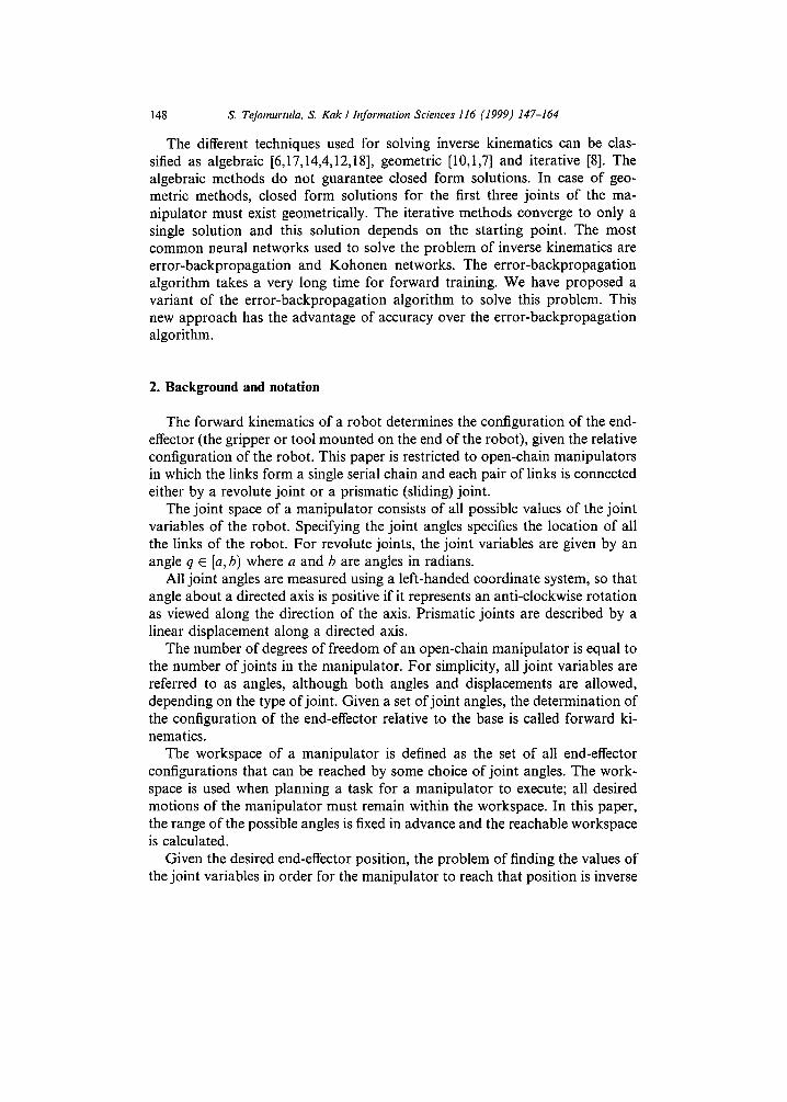
To illustrate some of the issues in inverse kinematics, consider the inverse kinematics of the planar two-link manipulator shown in Fig. 1.

The forward kinematics can be determined using plane geometry.

p, = L, cos(q,) + L2cos(q, + q2), (1)

P2 = L1 sin (ql) + Lzsin(ql + q2). (2)

The inverse problem is to solve for joint variables ql and q2, given the end- effector coordinates pl and Pz.

q2 = n rk a,

a = cos- ' ((L~ + L] - r2) / (2LIL2)) ,

ql = a tan(p2 ,p l ) 4- b,

b = cos- ' ((r 2 + L~ - L~) /2L , r ) .

(3)

(4)

(5)

(6)

L /

ss s~

Fig. 1. Inverse kinematics of a two-link manipulator.

150 s. Tejomurtula, S. Kak I hformation Sciences 116 (1999) 147-164

2.2. Different methods used for solv#zg inverse kinematics

The three main methods for solving inverse kinematics, namely, algebraic, geometric and iterative are described below.

Algebraic: Detailed steps toward an algebraic solution to the PUMA 500 manipulator can be found in Refs. [17,14,4]. To solve for inverse kinematics algebraically, it is necessary to solve equations q~,q2, . . . , qu for N degrees of freedom. The problem can be formulated as follows: given the end-effector position

= 0 0- l

(7)

where the right-hand side describes the required position and orientation of the end-effector. The problem comes down to solving N equations for N un- knowns [14]. This method does not guarantee a closed form solution for a given manipulator. Thus, engineers usually design simple manipulators where closed-form solutions exist.Craig [4], Manocha [12] and Zhu [18] proposed a generalized closed-form solution which can be derived for 6 (or less) DOF kinematic chain. Manocha [12] outlined a method for solving IK algebraically using symbolic manipulation to derive univariate polynomial and matrix computations.

Geometric: As opposed to the algebraic method, a closed form solution using the geometry of the manipulator is derived. Lee [10] used theorems in coordinate geometry which can be found in Ref. [1] to derive closed form solutions for a six DOF manipulator. This involves projecting of the link co- ordinate frame on the X~_l and Y~_l frame. This method can be applied to any manipulator with known geometry. The limitation of this method is that the closed-form solution for the first three joints of the manipulator must exist geometrically [7]. Apart from that, the closed-form solution for one class of manipulators cannot be used in other manipulators of a different geometry.

Iterative: This method solves inverse kinematics by iteratively solving for the joint angles. This method converges to only one solution as opposed to the two methods presented by Korein and Balder [8]. There are three components that constitute iterative methods, namely, the Jacobian, pseudo-inverse and mini- mization methods.

The inverse kinematics problem using neural networks comes under the class of iterative methods. They are however different from the conventional iterative methods used for solving inverse kinematics. It is important to note that the computational requirements are independent of the number of degrees of freedom of the robot arm; instead they are based on the network archi- tecture.

S. Tejomurtula, S. Kak I hformation Sciences 116 (1999) 147-164

3. Application of neural networks in inverse kinematics

151

In robotics, solving a problem using a programmed approach requires the development of software to implement the algorithm or set of rules. Frequently there are situations as in non-linear or complex multivariable systems, where the set of rules or required algorithms is unknown or too complex to be accurately modeled. Even if characterizing algorithms are obtained, they often are too computationally intensive for practical real-time applications. To circumvent this problem, neural networks are used. Neural networks are advantageous because they reduce software development, decrease computa- tional requirements, and allow for information processing capabilities where algorithms or rules are not known or cannot be derived.

The computational requirements for task and path planning, and path control, may be very demanding. However, robotic processes may be formu- lated in terms of optimization or pattern recognition problems so that neural network can be adapted.

3.1. Backpropagation

The conventional back-propagation algorithm is as follows: The number of hidden layers and the number of hidden neurons in each layer are decided. The network is fully connected between every two adjacent layers, i.e., the input neurons and the hidden neurons in the first hidden layer are fully connected. There is a connection between every pair of neurons between hidden layer 1 and hidden layer 2 and so on. The neurons in the final hidden layer are completely connected to the output layer. The weights of these connections are chosen at random. The first pattern is fed and its response is transported to the output layer. The error between the desired output and the actual output is propagated back. The weights are adjusted iteratively till the error falls below a threshold. Similarly all input patterns of the training set are fed and weights are adjusted. This process goes on till all the patterns are stored simultaneously.

The amount of time taken for training makes it practically useless for real time applications if the training set is very large.

3.2. Neural network inversions

The inversion problem for neural networks is to find inputs that yield a desired output [11]. There are three commonly used approaches for inverting networks. These are error back-propogation approach, the optimization ap- proach and the iterative approach based on update of input vector.

Optimization: In the optimization approach [9], the inversion problem is formulated as a non-linear programming problem. The neural network is trained using data points. Once the training is done, the weights are fixed. The

152 S. Tejomurtula, S. Kak / Information Sciences 116 (1999) 147-164

relation between every two hidden layers is approximated as a non-linear function. These equations are solved along with the constraint inequalities on the joint variables. A non-linear programming problem where the objective and the constraint functions can be expressed as a sum of functions, each in- volving only one variable, is called a non-linear separable programming problem. It can be approximated as a pseudo-linear programming problem and solved by a variation of the simplex method, a common technique for solving programming problems.

l terative: The neural network is trained using given data. Once the training is done, the weights are fixed. This method is based on the iterative update of an input node toward a solution, while escaping from local minima. The update rule is allowed to detect an input vector approaching a local mini- mum through a phenomenon called update explosion. At or near local minima, the input vector is guided by an escaping trajectory generated based on global information, which is predefined or known information on forward mapping.

Error Back-propagat ion: This algorithm works by adjusting the weights along the negative of the gradient in weight space of a standard error measure. The standard error can be the least-mean-square-error of the output. Using what is essentially the same back-propagation scheme, one may instead com- pute the gradient of this error measure in the space of input activation vectors; this gives rise to an algorithm for inverting the mapping performed by a net- work with specified weights. In this case the error is propagated back to the input units and it is the activation of these units - rather than the values of the weights in the network - that are adjusted so that a specified output pattern is evoked. The inversion is not unique for given targets and depends on the starting point in input space. The inversion tries to find an input pattern that generates a specific output pattern with the existing connections. To find the input, the deviation of each output from the desired output is computed as the error 6. The error value is used to approach the target input in input space step by step. The direction and length of this movement are computed by the in- version algorithm.

The most commonly used error value is the Leas t M e a n Square Error. E LMs is defined as

9

E LMs = Tp - f wijopi • (8) p=l

The goal of the algorithm, therefore, is to minimize E LMs . Since the error signal 6pl can be computed as

6pi : Opi(l -- Opi) Z 6pkWik (9) kESucc(i)

and for the adaption value of the unit activation follows

S. Tejomurtula, S. Kak / Information Sciences 116 (1999) 147-164 153

A netpi = rl6pi resp.netpi = netp/+ rl6pi. (10)

In this implementation, a uniform pattern is applied to the input units in the first step, whose activation level depends upon the variable input pattern. This pattern is propagated through the net and generates the initial output O (°). The difference between the output vector and the target output vector is propagated backwards through the net as error signal 61(0). This is analogous to propa- gation of error signals in backpropagation training, with the difference that no weights are adjusted here. When the error signals reach the input layer, they represent a gradient in the input space, which gives the direction for the gra- dient descent. Thereby, the new input vector can be computed as

i (1) = i(o) + ~/. 6~(o), (11)

where q is the step size in the input space. This procedure is now repeated with the new input vector until the distance between the generated output vector and the desired output vector falls below the predefined limit of 6m~x, when the algorithm is halted.

4. Solving inverse kinematics with backpropagation

The inversion with the conventional error-backpropagation algorithm is not unique for given targets and depends on the starting point in input space.

Lu and Ito [2] proposed the use of subnetworks to obtain more than one solution for a particular end-effector position. The configuration space was divided into N regions in a uniform or non-uniform grid. The data points were generated corresponding to each of the modular configuration spaces.

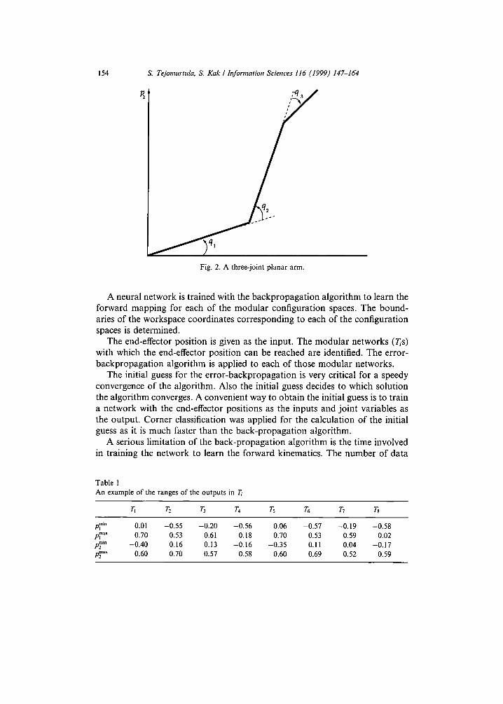
Fig. 2 shows a planar robot with three degrees of freedom [2] where the workspace (locus of the end-effector) is in a single plane. The angle q3 is marked negative because all the angles measured anticlockwise are positive. The lengths of the arms taken for simulation purposes are:

Ll =0.3, L2=0.25 L3=0.15.

The joint variables are fixed to be in the following ranges.

ql E [-z~/6, 2~/3], q2 E [0, 5r~/6], q3 E I-re/6, ~/6].

The forward kinematic equations of the model are as follows:

pt = LI cos(ql) + L2cos(ql + q2) + L3cos(ql + q2 + q3), (12)

P2 = L, sin (q~) + L2 sin(qt + q2) +L3 sin (q~ + q2 + q3). (13) The configuration space is divided into eight overlapping regions via the grid

points ( -~/6 , 3rc/12, 2rc/3), (0, 5~/12, 5~/6) and ( -~ /6 , 0, ~/6). For example, the first region is described by intervals [re/6, 3rc/12], [0, 5zc/12], and I-n/6,0]. Table 1 shows the ranges of the coordinates of the workspace T~, T2,..., Ts.

154 s. Tejomurtula, S. Kak I hTformation Sciences 116 (1999) 147-1~4

Fig. 2. A three-joint planar arm.

A neural network is trained with the backpropagat ion algorithm to learn the forward mapping for each of the modular configuration spaces. The bound- aries of the workspace coordinates corresponding to each of the configuration spaces is determined.

The end-effector position is given as the input. The modular networks (T~s) with which the end-effector position can be reached are identified. The error- backpropagat ion algorithm is applied to each of those modular networks.

The initial guess for the error-backpropagat ion is very critical for a speedy convergence of the algorithm. Also the initial guess decides to which solution the algorithm converges. A convenient way to obtain the initial guess is to train a network with the end-effector positions as the inputs and joint variables as the output. Corner classification was applied for the calculation of the initial guess as it is much faster than the back-propagat ion algorithm.

A serious limitation of the back-propagat ion algorithm is the time involved in training the network to learn the forward kinematics. The number of data

Table 1 An example of the ranges of the outputs in T~

T~ T_, 7"3 T4 7"5 7"6 /'7 T8

p]"~" 0.01 -0.55 -0.20 -0.56 0.06 -0.57 -0.19 -0.58 p~nax 0.70 0.53 0.61 0.18 0.70 0.53 0.59 0.02 p~i, -0.40 0.16 0.13 -0.16 -0.35 0,11 0.04 -0.17 pT "x 0.60 0.70 0.57 0.58 0.60 0.69 0.52 0.59

S. Tejomurtula, S. Kak / hfolvnation Sciences 116 (1999) 147-164 155

points for training cannot be reduced as accuracy is very critical in this ap- plication. Also forward kinematics can be determined for most of the existing models of the manipulators. The forward kinematics cannot be determined for some of the models having redundant joints. Even if the backpropagation network learns all the data points fed, it cannot beat the accuracy of the for- ward kinematic equation.

5. A new network architecture for error-backpropagation

Now we present our method which takes advantage of the fact that forward kinematics can be determined for most of the manipultors.

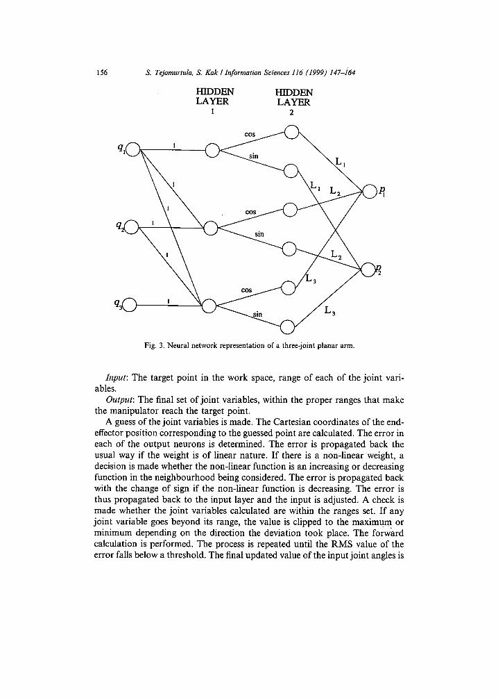
Any conventional network for backpropagation has weights that are real numbers. This network deviates from that common rule. The dimensions of the workspace are trigonometric functions of the joint variables. So some of the weights of the network are non-linear relationships of the nodes between which they are connected rather that real numbers. If there is a connection from node i in hidden layer 1 to node j in hidden layer 2 and the weight is say cosine, the value at node j in hidden layer 2 is cosine of the value at node i in hidden layer 1. Consider the example of the manipulator shown in Fig. 2. The position of the end-effector is given by the following set of equations:

Pl = Ll cos (ql) + L2 cos (ql + q2) + L3 cOS (ql + q2 + q3), (14)

P2 = Ll sin (ql) + Lz sin(ql + q2) + L3 sin(ql + q2 -k- q3), (15)

where ql, q2 and q3 are the joint variables, p~ and p2 are the coordinates of the end-effector, Lt,L2 and L3 are the lengths of the robot arms.

Instead of generating data of the joint variables and the Cartesian coordi- nates for training the network, the variables in the R.H.S of the equation i.e., L1, L2, L3, cos, sin are taken as the weights. The network architecture is as shown in Fig. 3.

Unlike the conventional back-propagation algorithm, no training is re- quired for this network. This network is different in the sense that some of the weights are non-linear functions of the nodes between which they are con- nected. So the error in the output layer cannot be propagated back the usual way.

5.1. The modified backpropagation

The neural network inversion for the error-backpropagation algorithm works as follows:

156 S. Tejomurtula, S. Kak / Information Sciences 116 (1999) 147-1~4

HIDDEN HIDDEN LAYER LAYER

I 2

qC) k._J ~ . ~ . ~ ~ L 3

Fig. 3. Neural network representation of a three-joint planar arm.

hTput: The target point in the work space, range of each of the joint vari- ables.

Output: The final set of joint variables, within the proper ranges that make the manipulator reach the target point.

A guess of the joint variables is made. The Cartesian coordinates of the end- effector position corresponding to the guessed point are calculated. The error in each of the output neurons is determined. The error is propagated back the usual way if the weight is of linear nature. If there is a non-linear weight, a decision is made whether the non-linear function is an increasing or decreasing function in the neighbourhood being considered. The error is propagated back with the change of sign if the non-linear function is decreasing. The error is thus propagated back to the input layer and the input is adjusted. A check is made whether the joint variables calculated are within the ranges set. If any joint variable goes beyond its range, the value is clipped to the maximum or minimum depending on the direction the deviation took place. The forward calculation is performed. The process is repeated until the RMS value of the error falls below a threshold. The final updated value of the input joint angles is

S. Tejomurtula, S. Kak I Information Sciences 116 (1999) 147-164 157

the desired result. The algorithm limits the final result to the subrange in which the guess is made. This algorithm does not require any extensive forward training as a backpropagation algorithm. It also does not have any encoding necessary as it takes in real values.

5.2. Modular networks

The partitioning of the joint space is done to get more than one solution, the forward kinematics of the model involve cosine and sine of the angles ql, ql + q2 and ql + q2 + q3. Since both the functions are decreasing or increasing de- pending on the value of the angle, the way the error needs be propagated from hidden layer 2 to hidden layer 1 (Fig. 3) depends on whether the cosine/sine is increasing or decreasing. The cosine or the sine of any angle changes sign at every integer multiple of n/2. So within the ranges of the angles qt, ql + q2, and ql + q2 + q3, the ranges are divided into smaller intervals with boundaries at the multiples of n/2. The point to which the algorithm converges depends on the initial guess. In order to evaluate the solutions for an end-effector position within the range of the angles, a guess is made for each of the increasing/de- creasing trend regions. The set of guesses is calculated as follows. In the model being considered, ql E [-n/6,2n/3]. There are two multiples of n/2 in the range. So the range is subdivided into [ -n /6 , 0], [0, n/2], [2n/3]. Similarly, the ranges ofql + q2 is divided into [-n/6, 0], [0, n/2], [n/2, n], [n, 3n/2]. The ranges of ql + q2 + q3 are I-n~3, 0], [0, n/2], [n/2, hi, [n, 3n/2], [3n/2, 5n/3]. n guess is a set of angles for qt, q2, q3. The guesses are made in such a way that all the angle ranges for qt, q~ + q2, qt + q2 + q3 are covered.

The ranges of the coordinates of the workspace (T~s) are calculated. An end- effector position is the input. All the subnets T~ within which the point lies are identified. It means that there may be zero, one or more solutions in this range. The other T~'s are ruled out. There may not be a solution in each of the sub- ranges.

6. Results with robots of different degrees of freedom and different types of joints

The algorithm was applied on different models of the manipulator. It could produce the solutions to a good degree of accuracy. The models and some of the results are as follows. The results for the remaining models can be obtained from [16].

6.1.. A planar robot with three degrees of freedom

The algorithm was applied to evaluate the inverse kinematic solutions of a planar robot with three degrees of freedom shown in Fig. 2. The accuracy of

158 s. Tejomurtula, S. Kak / Information Sciences 116 (1999) 147-16~I

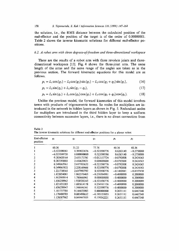
the solut ion, i.e., the R M S dis tance between the ca lcula ted pos i t ion o f the end-effector and the pos i t ion o f the target is o f the o rde r o f 0.00000001. Tab le 2 shows the inverse k inemat ic so lu t ions for different end-effector po- sit ions.

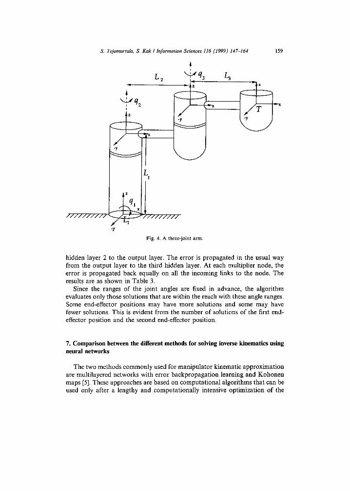
6.2. A robot arm with three degrees-of-freedom and three-dimentional workspace

These are the results o f a r o b o t a rm with three revolute jo in t s and three- d imen t iona l workspace [13]. Fig. 4 shows the three- jo in t arm. The same length o f the arms and the same range o f the angles are t aken as in the previous section. The fo rward k inemat ic equa t ions for this mode l are as follows.

Pl = Lt cos (ql) - Lzcos (q2)sin (ql) - L3 cos (q2 + q3)sin (ql) , (16)

P2 --- L2 sin (q2) +L3sin(q2 + q3), (17)

P3 = Lt sin(q1) + L 2 c o s ( q z ) c o s ( q l ) + Lacos (q2 + q3)cos(q l ) . (18)

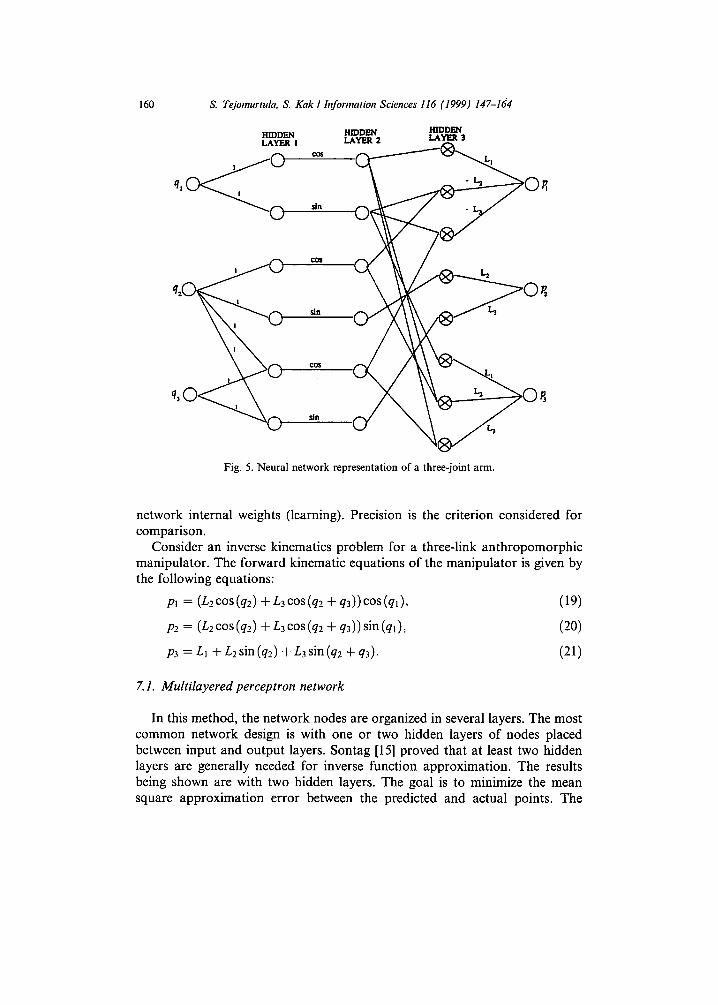
Unl ike the previous model , the fo rward k inemat ics o f this mode l involves terms with p roduc t s o f t r igonomet r ic terms. So nodes for mul t ip l iers are in- t roduced in the ne twork in h idden layers as shown in Fig. 5. R e d u n d a n t nodes for mul t ip l iers are in t roduced in the third h idden layer to keep a un i fo rm connect iv i ty between successive layers, i.e., there is no direct connec t ion f rom

Table 2 The inverse kinematic solutions for different end-effector positions for a planar robot

End-effector qt q2 q3 pl p,. position

1 60.36 51.23 77.76 60.36 60.36 1 -0.523598561 0.389823676 -0.523598776 0.6263140 -0.2750000 1 -0.523598720 0.000000000 0.523598586 0.6263140 -0.2750000 2 0.283428164 2.455173741 -0.012157724 -0.0792008 0.2424363 2 0.283392003 2.450629821 0.000000000 -0.0792008 0.2424363 2 0.349065961 2.617993632 -0.523598776 -0.0792008 0.2424363 2 0.349065822 2.228169666 0.523598776 -0.0792008 0.2424363 3 1.221730545 2.617993792 0.523598776 -0.1402081 -0.0197430 4 1.622054081 1.862576405 -0.239394981 -0.4000000 0.2000000 4 1.612918914 1.780666961 0.000000000 -0.4000000 0.2000000 4 1.656258942 1.938520345 -0.523598776 -0.4000000 0.2000000 4 1.621655383 1.685614178 0.234101156 -0.4000000 0.2000000 4 1.656258947 1.548696341 0.523598776 -0.4000000 0.2000000 5 1.101737701 0.144655985 0.000000000 0.2631111 0.6467348 5 1.178490703 0.083498632 -0.195153053 0.2631111 0.6467348 5 1.126387962 0.049447955 0.139242221 0.2631111 0.6467348

S. Tejomurtula, S. Kak I Information Sciences 116 (1999) 147-164 159

/ / / / / / / / / /

t

M.,,' q2 I I

-y

L I

-y

I

L 2 ~rJq3 [-'3

/ / / / / / / /

Fig. 4. A three-joint arm.

hidden layer 2 to the output layer. The error is propagated in the usual way from the output layer to the third hidden layer. At each multiplier node, the error is propagated back equally on all the incoming links to the node. The results are as shown in Table 3.

Since the ranges of the joint angles are fixed in advance, the algorithm evaluates only those solutions that are within the reach with these angle ranges. Some end-effector positions may have more solutions and some may have fewer solutions. This is evident from the number of solutions of the first end- effector position and the second end-effector position.

7. Comparison between the different methods for solving inverse kinematics using neural networks

The two methods commonly used for manipulator kinematic approximation are multilayered networks with error backpropagation learning and Kohonen maps [5]. These approaches are based on computational algorithms that can be used only after a lengthy and computationally intensive optimization of the

160 S. Tejomurtula, S. Kak I hzformation Sciences 116 (1999) 147-164

HIDDEN HIDDEN LAYER I I~'~:~R 2

0 a.

HIDDEN LAYER 9

Fig. 5. Neural network representation of a three-joint arm.

network internal weights (learning). Precision is the criterion considered for comparison.

Consider an inverse kinematics problem for a three-link anthropomorphic manipulator. The forward kinematic equations of the manipulator is given by the following equations:

Pl = (L2 cos (q2) + L3 cos (q2 + q3)) cos (ql),

P2 = (L2 c o s (q2) + L3 c o s (q2 + q3)) sin (ql),

P3 = L1 + L2 sin(q2) + L3 sin(q2 + q3).

(19)

(20)

(21)

7.1. Multilayered perceptron network

In this method, the network nodes are organized in several layers. The most common network design is with one or two hidden layers of nodes placed between input and output layers. Sontag [15] proved that at least two hidden layers are generally needed for inverse function approximation. The results being shown are with two hidden layers. The goal is to minimize the mean square approximation error between the predicted and actual points. The

S. Tejomurtula, S. Kak I Information Sciences 116 (1999) 147-164 161

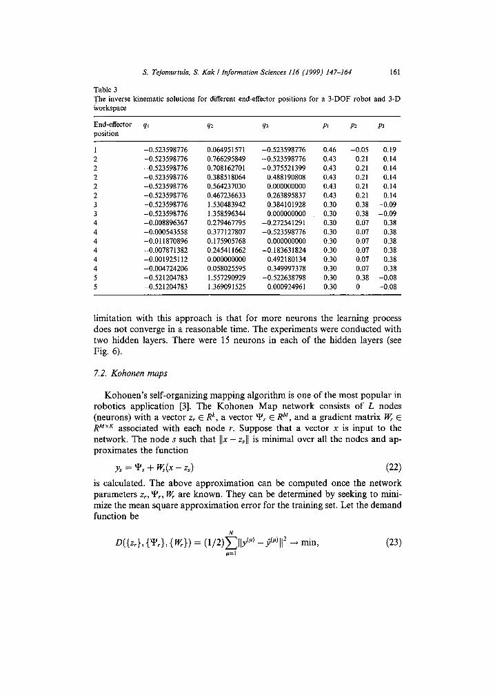
Table 3 The inverse kinematic solutions for different end-effector positions for a 3-DOF robot and 3-D

!

workspace

End-effector ql q2 q3 Pl P2_ P3 position

1 -0.523598776 0.064951571 -0.523598776 0.46 -0.05 0.19 2 -0.523598776 0.766295849 -0.523598776 0.43 0.21 0.14 2 -0.523598776 0.708162701 -0.375521399 0.43 0,21 0.14 2 -0.523598776 0.388518064 0.488190808 0.43 0.21 0.14 2 -0.523598776 0.564237030 0.000000000 0.43 0.21 0.14 2 -0.523598776 0.467236633 0.263895837 0.43 0.21 0.14 3 -0.523598776 1.530483942 -0.384101928 0.30 0.38 -0.09 3 -0.523598776 1.358596344 0.000000000 0.30 0.38 -0.09 4 -0.008896367 0.279467795 -0.272541291 0.30 0.07 0.38 4 -0.000543558 0.377127807 -0.523598776 0.30 0.07 0.38 4 -0.011870896 0.175905768 0.000000000 0.30 0.07 0.38 4 -0.007871382 0.245411662 -0.183631824 0.30 0.07 0.38 4 -0.001925112 0.000000000 0.492180134 0.30 0.07 0.38 4 -0.004724206 0.058025595 0.349997378 0.30 0.07 0.38 5 -0.521204783 1.557290929 -0.522638798 0.30 0.38 -0.08 5 -0.521204783 !.369091525 0.000924961 0.30 0 -0.08

limitation with this approach is that for more neurons the learning process does not converge in a reasonable time. The experiments were conducted with two hidden layers. There were 15 neurons in each of the hidden layers (see Fig. 6).

7.2. Kohonen maps

Kohonen's self-organizing mapping algorithm is one of the most popular in robotics application [3]. The Kohonen Map network consists of L nodes (neurons) with a vector z~ E R k, a vector tp~ E R M, and a gradient matrix W~ E R M×K associated with each node r. Suppose that a vector x is input to the network. The node s such that [ ix - zsi[ is minimal over all the nodes and ap- proximates the function

y, = it', + W,(x - z,) (22)

is calculated. The above approximation can be computed once the network parameters zr, ~,., W~ are known. They can be determined by seeking to mini- mize the mean square approximation error for the training set. Let the demand function be

N

D({zr}, {tpr}, { W~}) = (1/2)~- ']ly (') - p(U) ll ~ min, (23) ,u=l

162 S. Tejomurtula, S. Kak / Information Sciences 116 (1999) 147-164

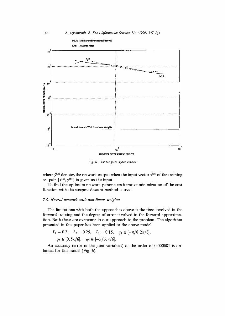
MLP: Multilayered Perceptron Network

KM: Kohonen Maps

I0

K.M

I0 . . . . . . . . . . . . . . . . . . . . . . . . . " . . . . . . . . . . . . . . . . . .

M L P

173v . . . . . . . . . . . . . . . . . . . . . . . . . . . . . . . . . . . . . . . . . . . . . . . . . . . . . . . . . . . . . . . . . . . . . . . . . : . . . . . . . . . . . . . . . . . . . . . . . . . . . . . . . . . . . . . . . . . . . . . . . . . . . . . . . . . . . . . . . . . . . . . . . . . e~

165 ....................................................................................................................................................

-6 Neural Network With Non-linear Weights 10

-7 10

I0 I I0 2 I0

N U M B E R O F T R A I N I N G POINTS

Fig. 6. Test set joint space errors.

where fi(") denotes the network output when the input vector x 0') of the training set pair {x("),y(")} is given as the input.

To find the optimum network parameters iterative minimization of the cost function with the steepest descent method is used.

7.3. N e u r a l network with non-linear weights

The limitations with both the approaches above is the time involved in the forward training and the degree of error involved in the forward approxima- tion. Both these are overcome in our approach to the problem. The algorithm presented in this paper has been applied to the above model.

L l = 0 . 3 , L2=0 .25 , L3=0 .15 , qlE[--rc/6,2rc/3],

q2 E [0, 5rc/6], q3 E [--~/6, rc/6].

An accuracy (error in the joint variables) of the order of 0.000001 is ob- tained for this model (Fig. 6).

S. Tejomurtula, S. Kak / Information Sciences 116 (1999) 147-164 163

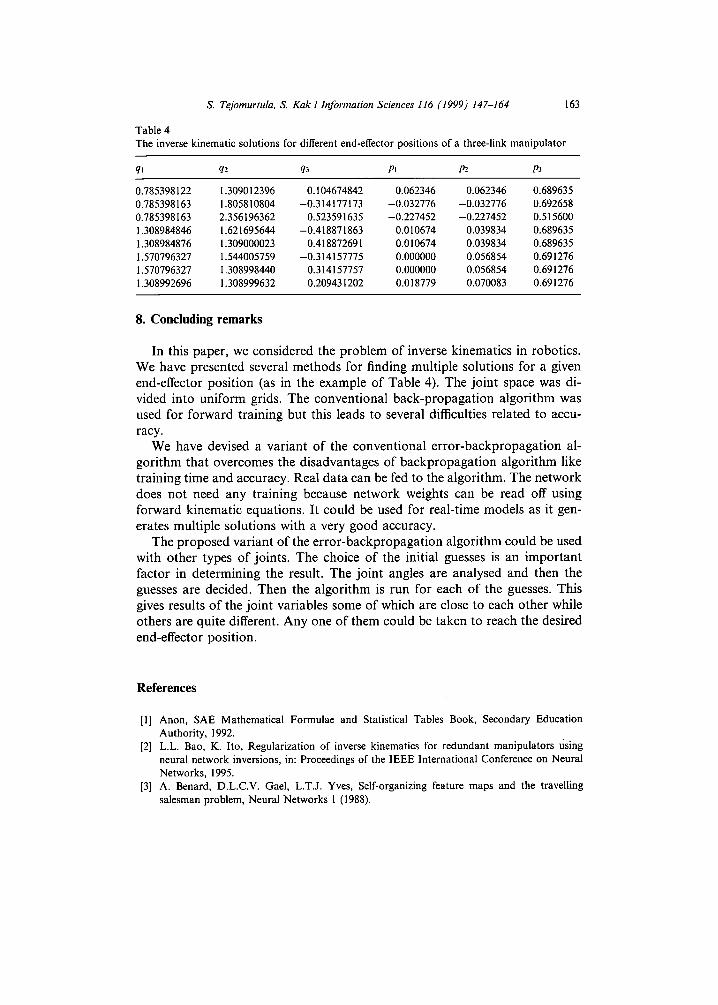
Table 4 The inverse kinematic solutions for different end-effector positions of a three-link manipulator

q~ q2 q3 pl P2_ P3

0.785398122 1 .309012396 0 .104674842 0 . 0 6 2 3 4 6 0 . 0 6 2 3 4 6 0.689635 0.785398163 1.805810804 -0.314177173 -0.032776 -0.032776 0.692658 0.785398163 2 .356196362 0 .523591635 -0.227452 -0.227452 0.515600 1.308984846 1.621695644 -0.418871863 0 . 0 1 0 6 7 4 0 . 0 3 9 8 3 4 0.689635 1.308984876 1 .309000023 0 .418872691 0 . 0 1 0 6 7 4 0 . 0 3 9 8 3 4 0.689635 1.570796327 1.544005759 -0.314157775 0 . 0 0 0 0 0 0 0 . 0 5 6 8 5 4 0.691276 1.570796327 1 .308998440 0 .314157757 0 . 0 0 0 0 0 0 0 . 0 5 6 8 5 4 0.691276 1.308992696 1 .308999632 0 .209431202 0 . 0 1 8 7 7 9 0 . 0 7 0 0 8 3 0.691276

8. Concluding remarks

In this paper, we considered the problem of inverse kinematics in robotics. We have presented several methods for finding multiple solutions for a given end-effector position (as in the example of Table 4). The joint space was di- vided into uniform grids. The conventional back-propagation algorithm was used for forward training but this leads to several difficulties related to accu- racy.

We have devised a variant of the conventional error-backpropagation al- gorithm that overcomes the disadvantages of backpropagation algorithm like training time and accuracy. Real data can be fed to the algorithm. The network does not need any training because network weights can be read off using forward kinematic equations. It could be used for real-time models as it gen- erates multiple solutions with a very good accuracy.

The proposed variant of the error-backpropagation algorithm could be used with other types of joints. The choice of the initial guesses is an important factor in determining the result. The joint angles are analysed and then the guesses are decided. Then the algorithm is run for each of the guesses. This gives results of the joint variables some of which are close to each other while others are quite different. Any one of them could be taken to reach the desired end-effector position.

References

[1] Anon, SAE Mathematical Formulae and Statistical Tables Book, Secondary Education Authority, 1992.

[2] L.L. Bao, K. Ito, Regularization of inverse kinematics for redundant manipulators using neural network inversions, in: Proceedings of the IEEE International Conference on Neural Networks, 1995.

[3] A. Benard, D.L.C.V. Gael, L.T.J. Yves, Self-organizing feature maps and the travelling salesman problem, Neural Networks 1 (1988).

164 S. Tejomurtula, S. Kak I h~formation Sciences 116 (1999) 147-164

[4] J.J. Craig, Introduction to Robotics: Mechanisms and Controls, Addison-Wesley, Reading, MA, 1989.

[5] Dimitri, Gorinevsky, T.H. Connoly, Comparison of some neural network and scattered data approximation: The inverse manipulator kinematics example, Neural Computation 6 (1994) 521-542.

[6] J. Duffy, Analysis of Mechanisms and Robot Manipulators, Wiley, New York, 1980. [7] R. Featherstone, Position and velocity transformation between robot end-effector coordinate

and joint angle, The International Journal of Robotics Research 2 (2) (1983) 35-45. [8] J.U. Korein, N.I. Balder, Techniques for generating the goal-directed motion of articulated

structures, IEEE Computer Graphics and Applications 2 (9) (1982) 71-81. [9] S. Lee, R.M. Kil, Inverse mapping of continuous functions using local and global information,

IEEE Transaction on Neural Networks 5 (1994)409-423. [10] G.C.S. Lee, Robot Arm Kinematics, Dynamics and Control, Computer 15 (12) (1982) 62-79. [11] A. Linden, J. Kindermann, Inverting of multilayer nets, IJCNN, 2 (1989). [12] D. Manocha, J.F. Canny, Efficient inverse kinematics for general 6r manipulators, IEEE

Transactions on Robotics and Automation 10 (5) (1994) 648-657. [13] R.M. Murray, Z. Li, S.S. Shastry, A Mathematical Introduction to Robotic Manipulation,

CRC Press, Boca Raton, 1994. [14] R.P. Paul, B. Shimano, G.E. Mayer, Kinematic control equations for simple manipulators,

IEEE Transactions on Systems, Man, and Cybernetics SMC-II (6) (1981) 66-72. [15] E.D. Sontag, Feedback stabilization using two-hidden layer nets, Rutgers Center for Systems

and Control, Rutgers University, New Brunswick, N J, 1990. [16] Sreenivas Tejomurtula, Inverse kinematics in robotics using neural networks, M.S. Thesis,

Louisiana State University, December, 1997. [17] W.E. Synder, Industrial Robots: Computer Interfacing and Control, Prentice-Hall, New

York, 1985. [18] D. Manocha, Y. Zhu, A fast algorithm and system for the inverse kinematics of general serial

manipulators, IEEE Conference on Robotics and Automation 94 (1994) 3348-3354.