Embed Size (px)
Citation preview
8/2/2019 InTech-Robot Kinematics Forward and Inverse Kinematics
http://slidepdf.com/reader/full/intech-robot-kinematics-forward-and-inverse-kinematics 1/32
8/2/2019 InTech-Robot Kinematics Forward and Inverse Kinematics
http://slidepdf.com/reader/full/intech-robot-kinematics-forward-and-inverse-kinematics 2/32
118 Industrial Robotics: Theory, Modelling and Control
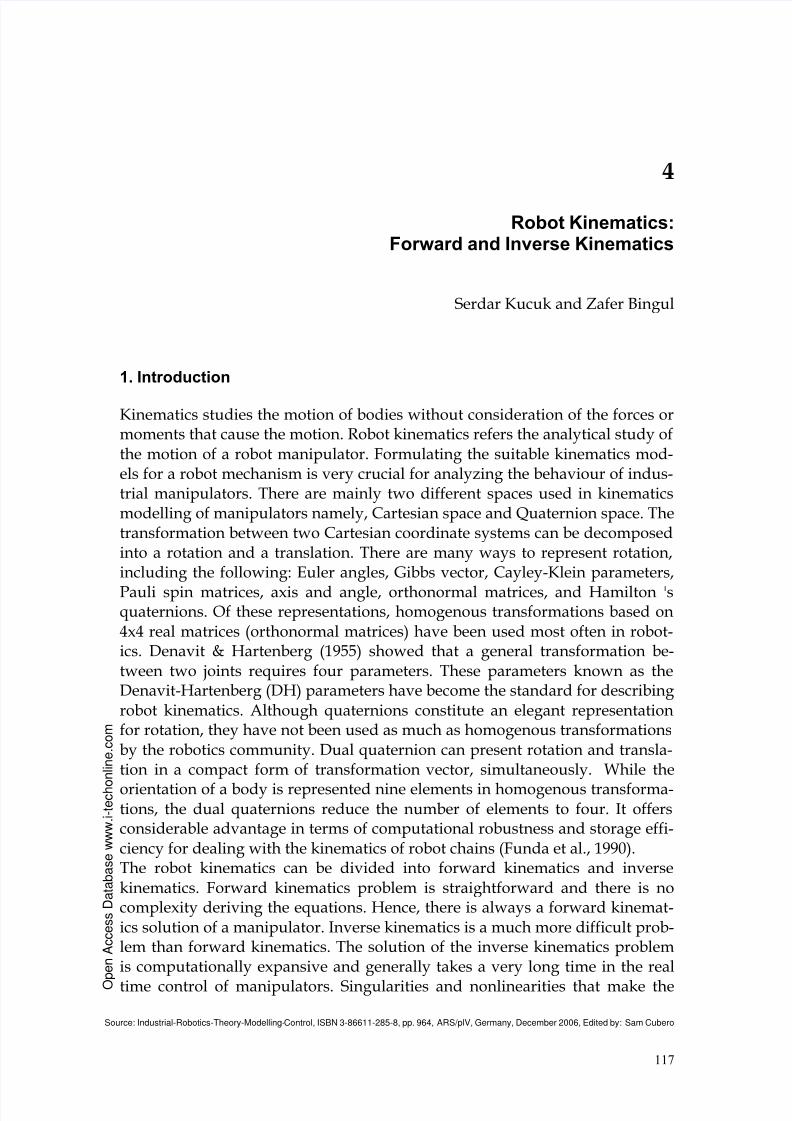
problem more difficult to solve. Hence, only for a very small class of kinemati-cally simple manipulators (manipulators with Euler wrist) have complete ana-
lytical solutions (Kucuk & Bingul, 2004). The relationship between forwardand inverse kinematics is illustrated in Figure 1.
Tn
θ1Forward kinematics
Inverse kinematics
Cartesian
space
Joint
space
θ2
θn
0.
Figure 10. The schematic representation of forward and inverse kinematics.
Two main solution techniques for the inverse kinematics problem are analyti-cal and numerical methods. In the first type, the joint variables are solved ana-lytically according to given configuration data. In the second type of solution,the joint variables are obtained based on the numerical techniques. In thischapter, the analytical solution of the manipulators is examined rather thennumerical solution.There are two approaches in analytical method: geometric and algebraic solu-tions. Geometric approach is applied to the simple robot structures, such as 2-DOF planar manipulator or less DOF manipulator with parallel joint axes. Forthe manipulators with more links and whose arms extend into 3 dimensions ormore the geometry gets much more tedious. In this case, algebraic approach ismore beneficial for the inverse kinematics solution.There are some difficulties to solve the inverse kinematics problem when thekinematics equations are coupled, and multiple solutions and singularities ex-ist. Mathematical solutions for inverse kinematics problem may not alwayscorrespond to the physical solutions and method of its solution depends on therobot structure.This chapter is organized in the following manner. In the first section, the for-ward and inverse kinematics transformations for an open kinematics chain aredescribed based on the homogenous transformation. Secondly, geometric andalgebraic approaches are given with explanatory examples. Thirdly, the prob-lems in the inverse kinematics are explained with the illustrative examples. Fi-nally, the forward and inverse kinematics transformations are derived basedon the quaternion modeling convention.
8/2/2019 InTech-Robot Kinematics Forward and Inverse Kinematics
http://slidepdf.com/reader/full/intech-robot-kinematics-forward-and-inverse-kinematics 3/32
Robot Kinematics: Forward and Inverse Kinematics 119
2. Homogenous Transformation Modelling Convention
2.1. Forward Kinematics
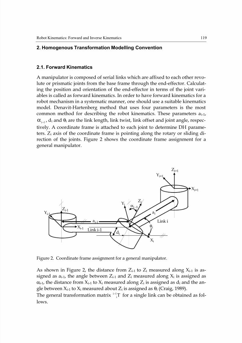
A manipulator is composed of serial links which are affixed to each other revo-lute or prismatic joints from the base frame through the end-effector. Calculat-ing the position and orientation of the end-effector in terms of the joint vari-ables is called as forward kinematics. In order to have forward kinematics for arobot mechanism in a systematic manner, one should use a suitable kinematicsmodel. Denavit-Hartenberg method that uses four parameters is the mostcommon method for describing the robot kinematics. These parameters a i-1,
1i−α , di and θi are the link length, link twist, link offset and joint angle, respec-tively. A coordinate frame is attached to each joint to determine DH parame-ters. Zi axis of the coordinate frame is pointing along the rotary or sliding di-rection of the joints. Figure 2 shows the coordinate frame assignment for ageneral manipulator.
1i−α
Link i-1
Yi-1
Zi-1
Xi-1
ai-1
di
YiZi
Xi
θi
Link i
ai
Yi+1
Zi+1
Xi+1
Figure 2. Coordinate frame assignment for a general manipulator.
As shown in Figure 2, the distance from Zi-1 to Zi measured along Xi-1 is as-signed as ai-1, the angle between Zi-1 and Zi measured along Xi is assigned as
αi-1, the distance from Xi-1 to Xi measured along Zi is assigned as di and the an-
gle between Xi-1 to Xi measured about Zi is assigned as θi (Craig, 1989).
The general transformation matrix T1i
i
− for a single link can be obtained as fol-
lows.
8/2/2019 InTech-Robot Kinematics Forward and Inverse Kinematics
http://slidepdf.com/reader/full/intech-robot-kinematics-forward-and-inverse-kinematics 4/32
120 Industrial Robotics: Theory, Modelling and Control
( ) ( ) ( ) ( )iiiz1ix1ix
1i
idQR aDR T θα=
−−
−
⎥⎥⎥⎥
⎦
⎤
⎢⎢⎢⎢
⎣
⎡
⎥⎥⎥⎥
⎦
⎤
⎢⎢⎢⎢
⎣
⎡
θθ
θ−θ
⎥⎥⎥⎥
⎦
⎤
⎢⎢⎢⎢
⎣
⎡
⎥⎥⎥⎥
⎦
⎤
⎢⎢⎢⎢
⎣
⎡
αα
α−α=
−
−−
−−
1000
d100
0010
0001
1000
0100
00cs
00sc
1000
0100
0010
a001
1000
0cs0
0sc0
0001
i
ii
ii1i
1i1i
1i1i
⎥
⎥⎥⎥
⎦
⎤
⎢
⎢⎢⎢
⎣
⎡
αααθαθ
α−α−αθαθ
θ−θ
=
−−−−
−−−−
−
1000
dccscss
dsscccs
a0sc
i1i1i1ii1ii
i1i1i1ii1ii
1iii
(1)
where Rx and Rz present rotation, Dx and Qi denote translation, and cθi and
sθi are the short hands of cosθi and sinθi, respectively. The forward kinematicsof the end-effector with respect to the base frame is determined by multiplying
all of the T1i
i
− matrices.
T...TTT 1n
n
1
2
0
1
base
effector _ end
−
= (2)
An alternative representation of T base
effector _ end can be written as
⎥⎥⎥⎥
⎦
⎤
⎢⎢⎢⎢
⎣
⎡
=−
1000
pr r r
pr r r
pr r r
Tz333231
y232221
x131211
base
effector end(3)
where rkj’s represent the rotational elements of transformation matrix (k and j=1, 2 and 3). px, py and pz denote the elements of the position vector. For a six jointed manipulator, the position and orientation of the end-effector with re-spect to the base is given by
)q(T)q(T)q(T)q(T)q(T)q(TT6
5
65
4
54
3
43
2
32
1
21
0
1
0
6= (4)
where qi is the joint variable (revolute or prismatic joint) for joint i, (i=1, 2, ..
.6).
8/2/2019 InTech-Robot Kinematics Forward and Inverse Kinematics
http://slidepdf.com/reader/full/intech-robot-kinematics-forward-and-inverse-kinematics 5/32
Robot Kinematics: Forward and Inverse Kinematics 121
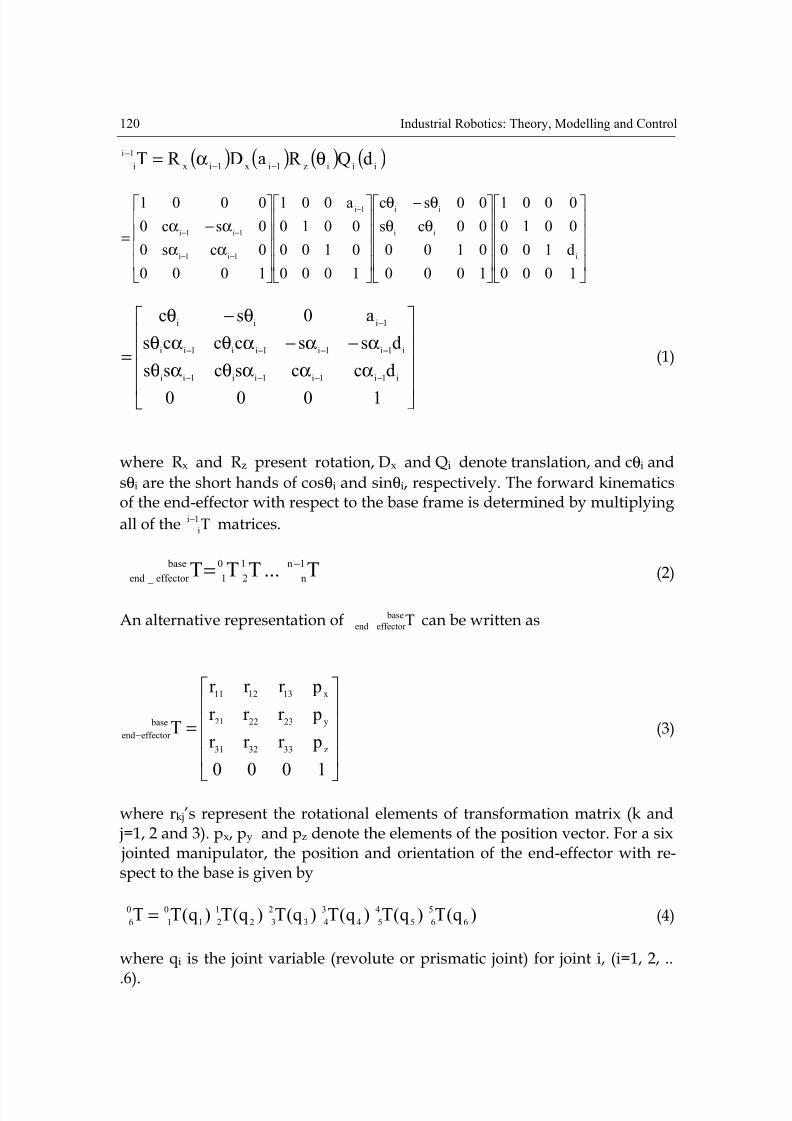
Example 1.As an example, consider a 6-DOF manipulator (Stanford Manipulator) whose
rigid body and coordinate frame assignment are illustrated in Figure 3. Notethat the manipulator has an Euler wrist whose three axes intersect at a com-mon point. The first (RRP) and last three (RRR) joints are spherical in shape. Pand R denote prismatic and revolute joints, respectively. The DH parameterscorresponding to this manipulator are shown in Table 1.
z 0,1
y2
x2
z2
z0
y0
d3
y3
z3
x3
θ1
θ2
x0
z1
y1
x1
h1
d2
θ4
θ5
θ6
z 4
x 4
y 4
z5
x 5
y5 z6
x 6
y6
Figure 3. Rigid body and coordinate frame assignment for the Stanford Manipulator.
i θi αi-1 ai-1 di
1 θ1 0 0 h1
2 θ2 90 0 d2
3 0 -90 0 d3
4 θ4 0 0 0
5 θ5 90 0 0
6 θ6 -90 0 0
Table 1. DH parameters for the Stanford Manipulator.
8/2/2019 InTech-Robot Kinematics Forward and Inverse Kinematics
http://slidepdf.com/reader/full/intech-robot-kinematics-forward-and-inverse-kinematics 6/32
122 Industrial Robotics: Theory, Modelling and Control
It is straightforward to compute each of the link transformation matrices usingequation 1, as follows.
⎥⎥⎥⎥
⎦
⎤
⎢⎢⎢⎢
⎣
⎡
θθ
θ−θ
=
1000
h100
00cs
00sc
T1
11
11
0
1
(5)
⎥
⎥⎥⎥
⎦
⎤
⎢
⎢⎢⎢
⎣
⎡
θθ
−−
θ−θ
=
1000
00cs
d100
00sc
T22
2
22
1
2
(6)
⎥⎥⎥⎥
⎦
⎤
⎢⎢⎢⎢
⎣
⎡
−=
1000
0010
d100
0001
T32
3
(7)
⎥⎥
⎥⎥
⎦
⎤
⎢⎢
⎢⎢
⎣
⎡
θθ
θ−θ
=
1000
0100
00cs
00sc
T44
44
3
4
(8)
⎥⎥⎥⎥
⎦
⎤
⎢⎢⎢⎢
⎣
⎡
θθ
−
θ−θ
=
1000
00cs
0100
00sc
T55
55
4
5
(9)
⎥⎥⎥⎥
⎦
⎤
⎢⎢⎢⎢
⎣
⎡
θ−θ−
θ−θ
=
1000
00cs
0100
00sc
T66
66
5
6
(10)
The forward kinematics of the Stanford Manipulator can be determined in the
form of equation 3 multiplying all of the T1i
i
− matrices, where i=1,2, …, 6. In
this case, T0
6 is given by
8/2/2019 InTech-Robot Kinematics Forward and Inverse Kinematics
http://slidepdf.com/reader/full/intech-robot-kinematics-forward-and-inverse-kinematics 7/32
Robot Kinematics: Forward and Inverse Kinematics 123
⎥⎥⎥
⎥
⎦
⎤
⎢⎢⎢
⎢
⎣
⎡
=
1000
pr r r
pr r r
pr r r
Tz333231
y232221
x131211
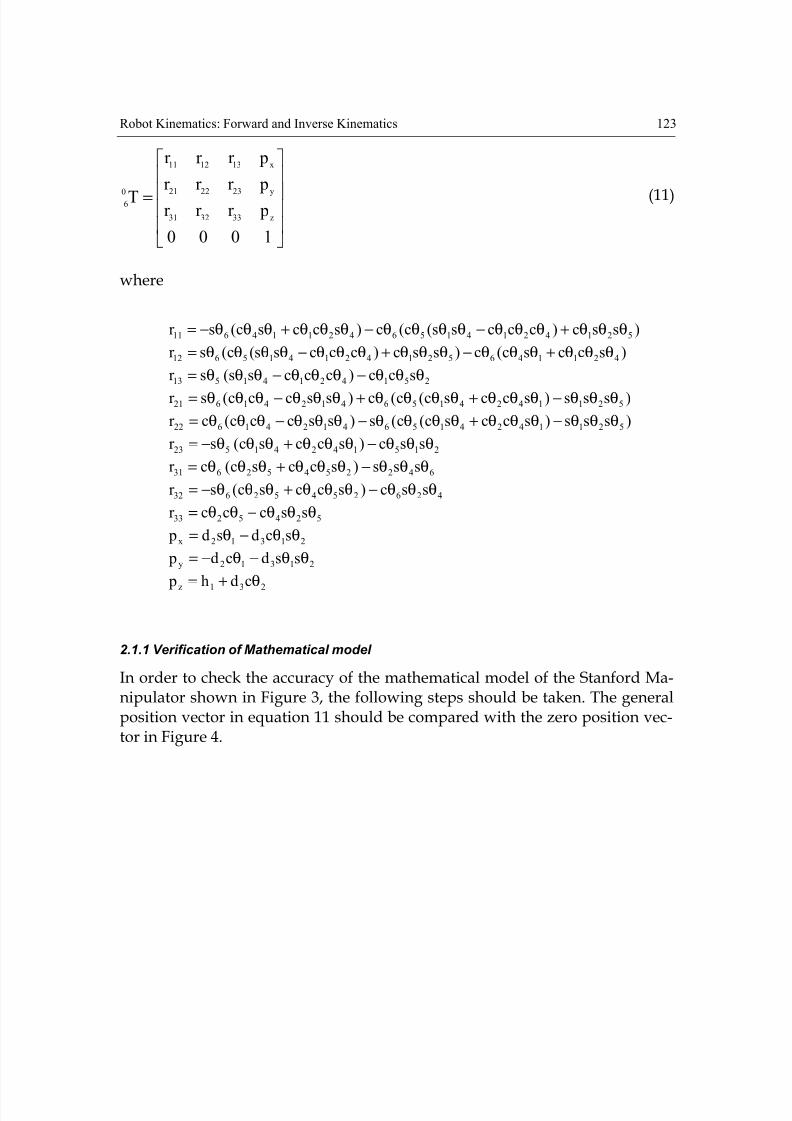
06 (11)
where
)ssc)cccss(c(c)sccsc(sr 521421415642114611 θθθ+θθθ−θθθθ−θθθ+θθθ−=
)sccsc(c)ssc)cccss(c(sr 421146521421415612 θθθ+θθθ−θθθ+θθθ−θθθθ=
25142141513 scc)cccss(sr θθθ−θθθ−θθθ=
)sss)sccsc(c(c)ssccc(sr 521142415641241621 θθθ−θθθ+θθθθ+θθθ−θθθ=
)sss)sccsc(c(s)ssccc(cr 521142415641241622 θθθ−θθθ+θθθθ−θθθ−θθθ=
21514241523 ssc)sccsc(sr θθθ−θθθ+θθθ−=
64225452631 sss)sccsc(cr θθθ−θθθ+θθθ=
42625452632 ssc)sccsc(sr θθθ−θθθ+θθθ−=
5245233 sscccr θθθ−θθ=
21312x scdsd p θθ−θ=
21312y ssdcd p θθ−θ−=
231z cdh pθ+=
2.1.1 Verification of Mathematical model
In order to check the accuracy of the mathematical model of the Stanford Ma-nipulator shown in Figure 3, the following steps should be taken. The generalposition vector in equation 11 should be compared with the zero position vec-tor in Figure 4.
8/2/2019 InTech-Robot Kinematics Forward and Inverse Kinematics
http://slidepdf.com/reader/full/intech-robot-kinematics-forward-and-inverse-kinematics 8/32
124 Industrial Robotics: Theory, Modelling and Control
z 0,1
h1
d2
d3
+z 0
+y0
+x0 -x0
-y0
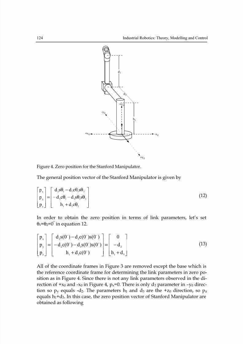
Figure 4. Zero position for the Stanford Manipulator.
The general position vector of the Stanford Manipulator is given by
⎥⎥⎥
⎦
⎤
⎢⎢⎢
⎣
⎡
θ+
θθ−θ−
θθ−θ
=
⎥⎥⎥
⎦
⎤
⎢⎢⎢
⎣
⎡
231
21312
21312
z
y
x
cdh
ssdcd
scdsd
p
p
p
(12)
In order to obtain the zero position in terms of link parameters, let’s set
θ1=θ2=0° in equation 12.
⎥⎥⎥
⎦
⎤
⎢⎢⎢
⎣
⎡
+
−=
⎥⎥⎥
⎦
⎤
⎢⎢⎢
⎣
⎡
+
−−
−
=
⎥⎥⎥
⎦
⎤
⎢⎢⎢
⎣
⎡
31
2
31
32
32
z
y
x
dh
d
0
)0(cdh
)0(s)0(sd)0(cd
)0(s)0(cd)0(sd
p
p
p
o
ooo
ooo
(13)
All of the coordinate frames in Figure 3 are removed except the base which isthe reference coordinate frame for determining the link parameters in zero po-sition as in Figure 4. Since there is not any link parameters observed in the di-rection of +x0 and -x0 in Figure 4, px=0. There is only d2 parameter in –y0 direc-tion so py equals -d2. The parameters h1 and d3 are the +z0 direction, so pz equals h1+d3. In this case, the zero position vector of Stanford Manipulator are
obtained as following
8/2/2019 InTech-Robot Kinematics Forward and Inverse Kinematics
http://slidepdf.com/reader/full/intech-robot-kinematics-forward-and-inverse-kinematics 9/32
Robot Kinematics: Forward and Inverse Kinematics 125
⎥⎥⎥
⎦
⎤
⎢⎢⎢
⎣
⎡
+
−=
⎥⎥⎥
⎦
⎤
⎢⎢⎢
⎣
⎡
31
2
z
y
x
dh
d
0
p
p
p
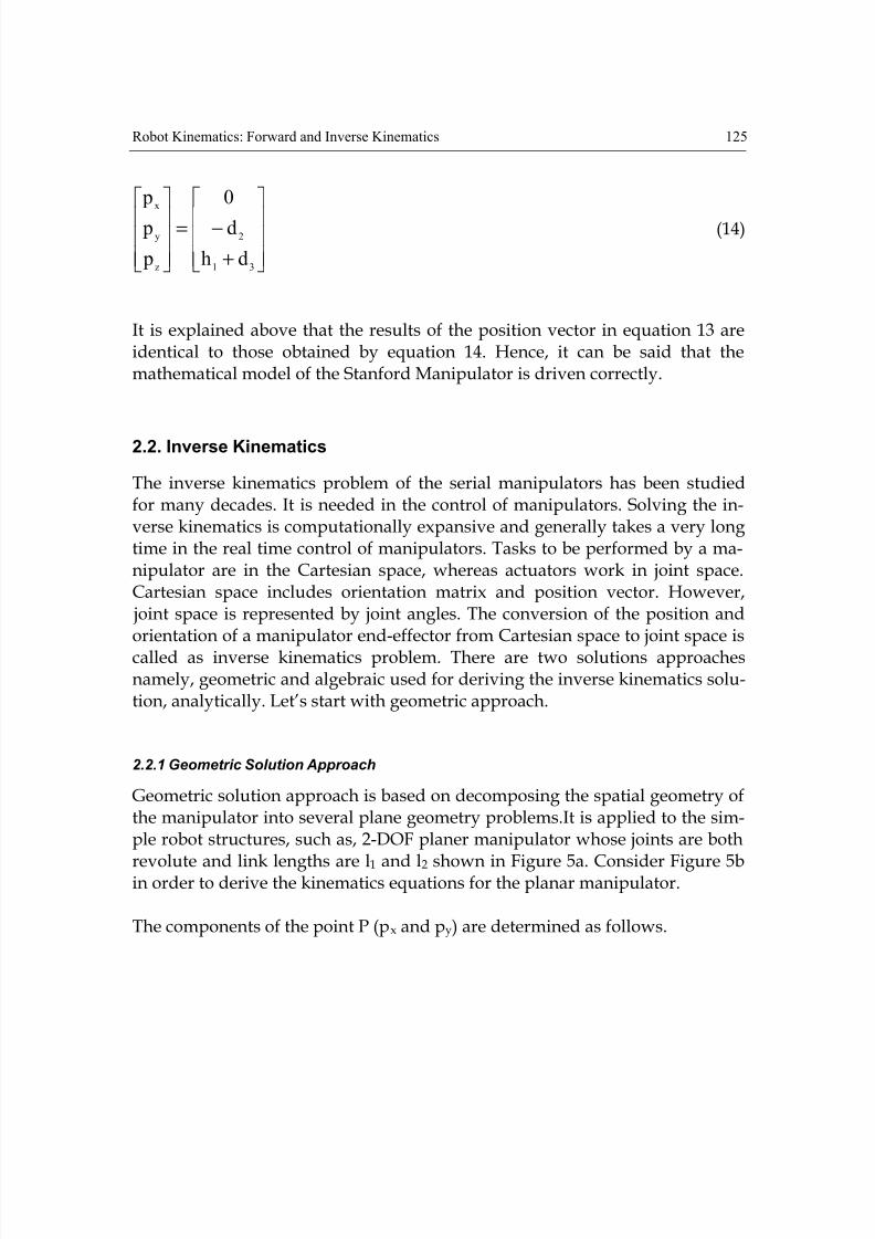
(14)
It is explained above that the results of the position vector in equation 13 areidentical to those obtained by equation 14. Hence, it can be said that themathematical model of the Stanford Manipulator is driven correctly.
2.2. Inverse Kinematics
The inverse kinematics problem of the serial manipulators has been studiedfor many decades. It is needed in the control of manipulators. Solving the in-verse kinematics is computationally expansive and generally takes a very longtime in the real time control of manipulators. Tasks to be performed by a ma-nipulator are in the Cartesian space, whereas actuators work in joint space.Cartesian space includes orientation matrix and position vector. However,
joint space is represented by joint angles. The conversion of the position andorientation of a manipulator end-effector from Cartesian space to joint space is
called as inverse kinematics problem. There are two solutions approachesnamely, geometric and algebraic used for deriving the inverse kinematics solu-tion, analytically. Let’s start with geometric approach.
2.2.1 Geometric Solution Approach
Geometric solution approach is based on decomposing the spatial geometry ofthe manipulator into several plane geometry problems.It is applied to the sim-ple robot structures, such as, 2-DOF planer manipulator whose joints are both
revolute and link lengths are l1 and l2 shown in Figure 5a. Consider Figure 5bin order to derive the kinematics equations for the planar manipulator.
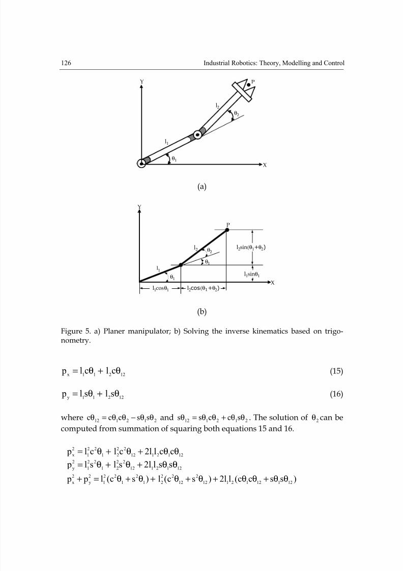
The components of the point P (px and py) are determined as follows.
8/2/2019 InTech-Robot Kinematics Forward and Inverse Kinematics
http://slidepdf.com/reader/full/intech-robot-kinematics-forward-and-inverse-kinematics 10/32
126 Industrial Robotics: Theory, Modelling and Control
l1
θ1
θ2
l2
X
Y P
(a)
Y
θ2
θ1
θ1
l1
l2
Xl1cosθ1 l2cos(θ1+θ2)
l1sinθ1
l2sin(θ1+θ2)
P
(b)
Figure 5. a) Planer manipulator; b) Solving the inverse kinematics based on trigo-nometry.
12211xclcl p θ+θ= (15)
12211yslsl p θ+θ= (16)
where 212112 ssccc θθ−θθ=θ and 212112 sccss θθ+θθ=θ . The solution of 2θ can be
computed from summation of squaring both equations 15 and 16.
1212112
22
21
22
1
2
xccll2clcl p θθ+θ+θ=
1212112
22
21
22
1
2
yssll2slsl p θθ+θ+θ=
)sscc(ll2)sc(l)sc(l p p1211212112
2
12
22
21
2
1
22
1
2
y
2
xθθ+θθ+θ+θ+θ+θ=+
8/2/2019 InTech-Robot Kinematics Forward and Inverse Kinematics
http://slidepdf.com/reader/full/intech-robot-kinematics-forward-and-inverse-kinematics 11/32
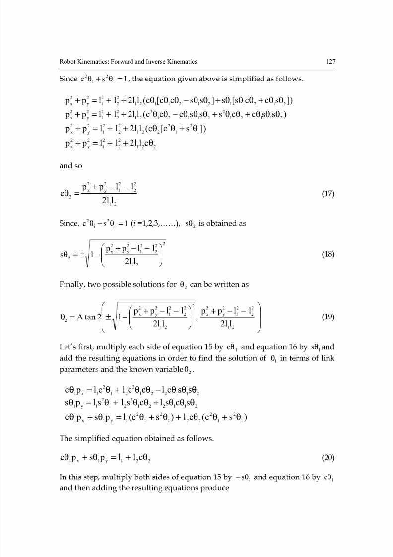
Robot Kinematics: Forward and Inverse Kinematics 127
Since 1sc 1
2
1
2=θ+θ , the equation given above is simplified as follows.
])sccs[s]sscc[c(ll2ll p p 21211212112122
21
2y
2x θθ+θθθ+θθ−θθθ++=+
)ssccsssccc(ll2ll p p21121
2
21121
2
21
2
2
2
1
2
y
2
xθθθ+θθ+θθθ−θθ++=+
])sc[c(ll2ll p p1
2
1
2
221
2
2
2
1
2
y
2
xθ+θθ++=+
221
2
2
2
1
2
y
2
xcll2ll p p θ++=+
and so
21
2
2
2
1
2
y
2
x
2ll2
ll p p
c
−−+
=θ (17)
Since, 1sc i
2
i
2=θ+θ (i =1,2,3,……), 2sθ is obtained as
2
21
2
2
2
1
2
y
2
x
2ll2
ll p p1s ⎟⎟
⎠
⎞⎜⎜⎝
⎛ −−+−±=θ (18)
Finally, two possible solutions for 2θ can be written as
⎟⎟
⎠
⎞
⎜⎜
⎝
⎛ −−+
⎟⎟ ⎠
⎞⎜⎜⎝
⎛ −−+−±=θ
21
2
2
2
1
2
y
2
x
2
21
2
2
2
1
2
y
2
x
2ll2
ll p p,
ll2
ll p p12tanA (19)
Let’s first, multiply each side of equation 15 by 1cθ and equation 16 by 1sθ and
add the resulting equations in order to find the solution of 1θ in terms of link
parameters and the known variable 2θ .
211221
2
21
2
1x1 ssclcclcl pc θθθ−θθ+θ=θ
211221
2
21
2
1y1scslcslsl ps θθθ+θθ+θ=θ
)sc(cl)sc(l ps pc1
2
1
2
221
2
1
2
1y1x1θ+θθ+θ+θ=θ+θ
The simplified equation obtained as follows.
221y1x1cll ps pc θ+=θ+θ (20)
In this step, multiply both sides of equation 15 by 1sθ− and equation 16 by 1cθ
and then adding the resulting equations produce
8/2/2019 InTech-Robot Kinematics Forward and Inverse Kinematics
http://slidepdf.com/reader/full/intech-robot-kinematics-forward-and-inverse-kinematics 12/32
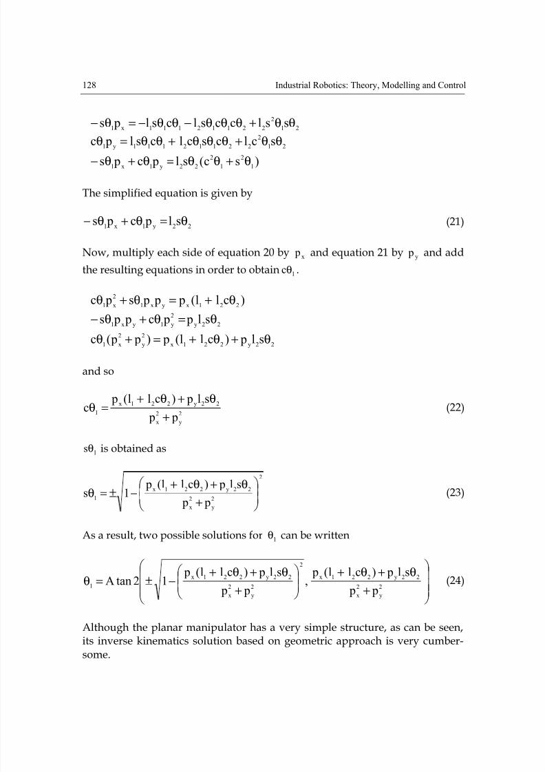
128 Industrial Robotics: Theory, Modelling and Control
21
2
22112111x1sslccslcsl ps θθ+θθθ−θθ−=θ−
21
2
22112111y1sclcsclcsl pc θθ+θθθ+θθ=θ
)sc(sl pc ps1
2
1
2
22y1x1θ+θθ=θ+θ−
The simplified equation is given by
22y1x1sl pc ps θ=θ+θ− (21)
Now, multiply each side of equation 20 by x p and equation 21 by y p and add
the resulting equations in order to obtain 1cθ .
)cll( p p ps pc221xyx1
2
x1θ+=θ+θ
22y
2
y1yx1sl p pc p ps θ=θ+θ−
22y221x
2
y
2
x1sl p)cll( p) p p(c θ+θ+=+θ
and so
2
y
2
x
22y221x1
p p
sl p)cll( pc
+
θ+θ+
=θ (22)
1sθ is obtained as
2
2
y
2
x
22y221x
1 p p
sl p)cll( p1s ⎟
⎟ ⎠
⎞
⎜⎜⎝
⎛
+
θ+θ+−±=θ (23)
As a result, two possible solutions for 1θ
can be written
⎟⎟⎟
⎠
⎞
⎜⎜⎜
⎝
⎛
+
θ+θ+
⎟⎟
⎠
⎞
⎜⎜
⎝
⎛
+
θ+θ+−±=θ
2
y
2
x
22y221x
2
2
y
2
x
22y221x
1 p p
sl p)cll( p,
p p
sl p)cll( p12tanA (24)
Although the planar manipulator has a very simple structure, as can be seen,its inverse kinematics solution based on geometric approach is very cumber-some.
8/2/2019 InTech-Robot Kinematics Forward and Inverse Kinematics
http://slidepdf.com/reader/full/intech-robot-kinematics-forward-and-inverse-kinematics 13/32
Robot Kinematics: Forward and Inverse Kinematics 129
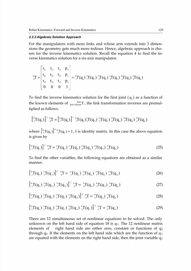
2.2.2 Algebraic Solution Approach
For the manipulators with more links and whose arm extends into 3 dimen-
sions the geometry gets much more tedious. Hence, algebraic approach is cho-sen for the inverse kinematics solution. Recall the equation 4 to find the in-verse kinematics solution for a six-axis manipulator.
)q(T)q(T)q(T)q(T)q(T)q(T
1000
pr r r
pr r r
pr r r
T6
5
65
4
54
3
43
2
32
1
21
0
1
z333231
y232221
x131211
0
6=
⎥⎥⎥⎥
⎦
⎤
⎢⎢⎢⎢
⎣
⎡
=
To find the inverse kinematics solution for the first joint ( 1q ) as a function of
the known elements of T base
effector end− , the link transformation inverses are premul-
tiplied as follows.
[ ] [ ] )q(T)q(T)q(T)q(T)q(T)q(T)q(TT)q(T6
5
65
4
54
3
43
2
32
1
21
0
1
1
1
0
1
0
6
1
1
0
1
−−
=
where [ ] I)q(T)q(T 1
0
1
1
1
0
1 =−
, I is identity matrix. In this case the above equation
is given by
[ ] )q(T)q(T)q(T)q(T)q(TT)q(T6
5
65
4
54
3
43
2
32
1
2
0
6
1
1
0
1=
−
(25)
To find the other variables, the following equations are obtained as a similarmanner.
[ ] )q(T)q(T)q(T)q(TT)q(T)q(T6
5
65
4
54
3
43
2
3
0
6
1
2
1
21
0
1=
−
(26)
[ ] )q(T)q(T)q(TT)q(T)q(T)q(T6
5
65
4
54
3
4
0
6
1
3
2
32
1
21
0
1=
−
(27)
[ ] )q(T)q(TT)q(T)q(T)q(T)q(T6
5
65
4
5
0
6
1
4
3
43
2
32
1
21
0
1=
−
(28)
[ ] )q(TT)q(T)q(T)q(T)q(T)q(T6
5
6
0
6
1
5
4
54
3
43
2
32
1
21
0
1=
−
(29)
There are 12 simultaneous set of nonlinear equations to be solved. The onlyunknown on the left hand side of equation 18 is q1. The 12 nonlinear matrixelements of right hand side are either zero, constant or functions of q2 through q6. If the elements on the left hand side which are the function of q 1
are equated with the elements on the right hand side, then the joint variable q1
8/2/2019 InTech-Robot Kinematics Forward and Inverse Kinematics
http://slidepdf.com/reader/full/intech-robot-kinematics-forward-and-inverse-kinematics 14/32
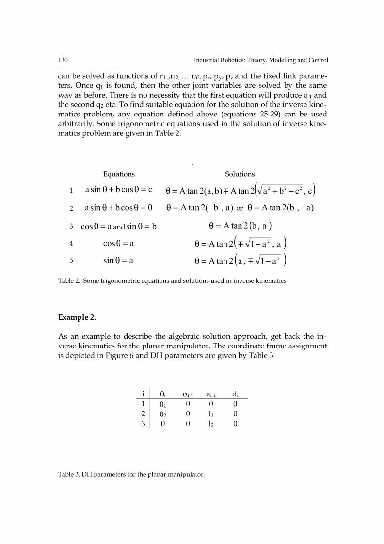
130 Industrial Robotics: Theory, Modelling and Control
can be solved as functions of r11,r12, … r33, px, py, pz and the fixed link parame-ters. Once q1 is found, then the other joint variables are solved by the same
way as before. There is no necessity that the first equation will produce q 1 andthe second q2 etc. To find suitable equation for the solution of the inverse kine-matics problem, any equation defined above (equations 25-29) can be usedarbitrarily. Some trigonometric equations used in the solution of inverse kine-matics problem are given in Table 2.
.
Equations Solutions
1 ccos bsina =θ+θ )c,c ba2tanA) b,a(2tanA 222 −+=θ m
2 0cos bsina =θ+θ )a, b(2tanA −=θ or )a, b(2tanA −=θ
3 acos =θ and bsin =θ ( )a, b2tanA=θ
4 acos =θ )a,a12tanA 2−=θ m
5 asin =θ ( )2a1,a2tanA −=θ m
Table 2. Some trigonometric equations and solutions used in inverse kinematics
Example 2.
As an example to describe the algebraic solution approach, get back the in-verse kinematics for the planar manipulator. The coordinate frame assignmentis depicted in Figure 6 and DH parameters are given by Table 3.
i θi αi-1 ai-1 di
1 θ1 0 0 0
2 θ2 0 l1 0
3 0 0 l2 0
Table 3. DH parameters for the planar manipulator.
8/2/2019 InTech-Robot Kinematics Forward and Inverse Kinematics
http://slidepdf.com/reader/full/intech-robot-kinematics-forward-and-inverse-kinematics 15/32
Robot Kinematics: Forward and Inverse Kinematics 131
l1
θ1
θ2
l2
X0,1
Y0,1
Z0,1
X2
Y2
Z2
X3
Y3
Z3
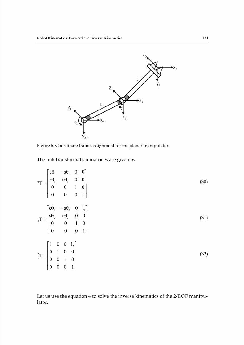
Figure 6. Coordinate frame assignment for the planar manipulator.
The link transformation matrices are given by
⎥⎥⎥
⎥
⎦
⎤
⎢⎢⎢
⎢
⎣
⎡
θθ
θ−θ
=
1000
010000cs
00sc
T 11
11
0
1(30)
⎥⎥⎥⎥
⎦
⎤
⎢⎢⎢⎢
⎣
⎡
θθ
θ−θ
=
1000
0100
00cs
l0sc
T22
122
1
2
(31)
⎥⎥⎥⎥
⎦
⎤
⎢⎢⎢⎢
⎣
⎡
=
1000
0100
0010
l001
T
2
2
3
(32)
Let us use the equation 4 to solve the inverse kinematics of the 2-DOF manipu-
lator.
8/2/2019 InTech-Robot Kinematics Forward and Inverse Kinematics
http://slidepdf.com/reader/full/intech-robot-kinematics-forward-and-inverse-kinematics 16/32
132 Industrial Robotics: Theory, Modelling and Control
TTT
1000
pr r r
pr r r
pr r r
T 2
3
1
2
0
1
z333231
y232221
x131211
0
3=
⎥⎥⎥⎥
⎦
⎤
⎢⎢⎢⎢
⎣
⎡
= (33)
Multiply each side of equation 33 by 10
1T−
TTTTTT 2
3
1
2
0
1
10
1
0
3
10
1
−−= (34)
where
⎥⎦
⎤⎢⎣
⎡ −=
−
1000
PR R T 1
0T0
1
T0
110
1(35)
In equation 35, T0
1 R and 1
0 P denote the transpose of rotation and position vec-
tor of T0
1 , respectively. Since, ITT0
1
10
1 =− , equation 34 can be rewritten as fol-
lows.
TTTT 2
3
1
2
0
3
10
1=
−(36)
Substituting the link transformation matrices into equation 36 yields
⎥⎥⎥⎥
⎦
⎤
⎢⎢⎢⎢
⎣
⎡
⎥⎥⎥⎥
⎦
⎤
⎢⎢⎢⎢
⎣
⎡
θθ
θ−θ
=
⎥⎥⎥⎥
⎦
⎤
⎢⎢⎢⎢
⎣
⎡
⎥⎥⎥⎥
⎦
⎤
⎢⎢⎢⎢
⎣
⎡
θθ−
θθ
1000
0100
0010
l001
1000
0100
00cs
l0sc
1000
pr r r
pr r r
pr r r
1000
0100
00cs
00sc2
22
122
z333231
y232221
x131211
11
11
(37)
⎥⎥⎥⎥
⎦
⎤
⎢⎢⎢⎢
⎣
⎡
θ
+θ
=
⎥⎥⎥⎥
⎦
⎤
⎢⎢⎢⎢
⎣
⎡
θ+θ−
θ+θ
1000
0...
sl...
lcl...
1000
p...
pc ps...
ps pc...
22
122
z
y1x1
y1x1
Squaring the (1,4) and (2,4) matrix elements of each side in equation 37
8/2/2019 InTech-Robot Kinematics Forward and Inverse Kinematics
http://slidepdf.com/reader/full/intech-robot-kinematics-forward-and-inverse-kinematics 17/32
Robot Kinematics: Forward and Inverse Kinematics 133
2
12212
22
211yx
2
y1
22
x1
2 lcll2clsc p p2 ps pc +θ+θ=θθ+θ+θ
2
22
211yx
2
y1
22
x1
2
slsc p p2 pc psθ=θθ−θ+θ
and then adding the resulting equations above gives
2
12212
2
2
22
21
2
1
22
y1
2
1
22
xlcll2)sc(l)cs( p)sc( p +θ+θ+θ=θ+θ+θ+θ
2
1221
2
2
2
y
2
xlcll2l p p +θ+=+
21
2
2
2
1
2
y
2
x
2ll2
ll p pc
−−+=θ
Finally, two possible solutions for 2θ are computed as follows using the fourth
trigonometric equation in Table 2.
⎟⎟⎟
⎠
⎞
⎜⎜⎜
⎝
⎛ −−+
⎥⎦
⎤⎢⎣
⎡ −−+−=θ
21
2
2
2
1
2
y
2
x
2
21
2
2
2
1
2
y
2
x
2ll2
ll p p,
ll2
ll p p12tanA m (38)
Now the second joint variable 2θ is known. The first joint variable 1θ can be
determined equating the (1,4) elements of each side in equation 37 as follows.
122y1x1lcl ps pc +θ=θ+θ (39)
Using the first trigonometric equation in Table 2 produces two potential solu-tions.
)lcl,)lcl( p p(2tanA) p, p(2tanA122
2
122x
2
yxy1+θ+θ−+=θ m (40)
Example 3.
As another example for algebraic solution approach, consider the six-axis Stan-ford Manipulator again. The link transformation matrices were previously de-veloped. Equation 26 can be employed in order to develop equation 41. Theinverse kinematics problem can be decoupled into inverse position and orien-tation kinematics. The inboard joint variables (first three joints) can be solvedusing the position vectors of both sides in equation 41.
[ ] TTTTTTT 5
6
4
5
3
4
2
3
0
6
11
2
0
1
=−
(41)
8/2/2019 InTech-Robot Kinematics Forward and Inverse Kinematics
http://slidepdf.com/reader/full/intech-robot-kinematics-forward-and-inverse-kinematics 18/32
134 Industrial Robotics: Theory, Modelling and Control
⎥⎥⎥
⎥
⎦
⎤
⎢⎢⎢
⎢
⎣
⎡
=
⎥⎥⎥
⎥
⎦
⎤
⎢⎢⎢
⎢
⎣
⎡
−θ−θ
−θ+θ+θθ−
−θ+θ+θθ
1000
0...
d...
0...
1000
d pc ps...
)h p(c) ps pc(s...
)h p(s) ps pc(c...
3
2y1x1
1z2y1x12
1z2y1x12
The revolute joint variables 1θ and 2θ are obtained equating the (3,4) and (1,4)
elements of each side in equation 41 and using the first and second trigono-metric equations in Table 2, respectively.
)d,d p p(2tanA) p, p(2tanA2
2
2
2
y
2
xyx1−+±−=θ (42)
)h p, ps pc(2tanA 1zy1x12 +−θ+θ±=θ (43)
The prismatic joint variable 3d is extracted from the (2,4) elements of each side
in equation 41 as follows.
)h p(c) ps pc(sd1z2y1x123
−θ+θ+θθ−= (44)
The last three joint variables may be found using the elements of rotation ma-
trices of each side in equation 41. The rotation matrices are given by
⎥⎥⎥⎥
⎦
⎤
⎢⎢⎢⎢
⎣
⎡
θθ
θθθ−θθ
θθ−
=
⎥⎥⎥⎥
⎦
⎤
⎢⎢⎢⎢
⎣
⎡
θ−θ
θθ−θθ−θ
θθ+θθ+θ
1000
.ss..
.csssc
.sc..
1000
.cr sr ..
.ssr scr cr ed
.scr ccr sr ..
54
56556
54
123113
21232113233
12232113233
(45)
where 21212111231 ssr scr cr d θθ−θθ−θ= and 21222112232 ssr scr cr e θθ−θθ−θ= . The
revolute joint variables 5θ is determined equating the (2,3) elements of both
sides in equation 45 and using the fourth trigonometric equation in Table 2, asfollows.
( )21232113233
2
212321132335ssr scr cr ,)ssr scr cr (12tanA θθ−θθ−θθθ−θθ−θ−±=θ (46)
Extracting 4cosθ and 4sinθ from (1,3) and (3,3), 6cosθ and 6sinθ from (2,1)
and (2,2) elements of each side in equation 45 and using the third trigonomet-
8/2/2019 InTech-Robot Kinematics Forward and Inverse Kinematics
http://slidepdf.com/reader/full/intech-robot-kinematics-forward-and-inverse-kinematics 19/32
Robot Kinematics: Forward and Inverse Kinematics 135
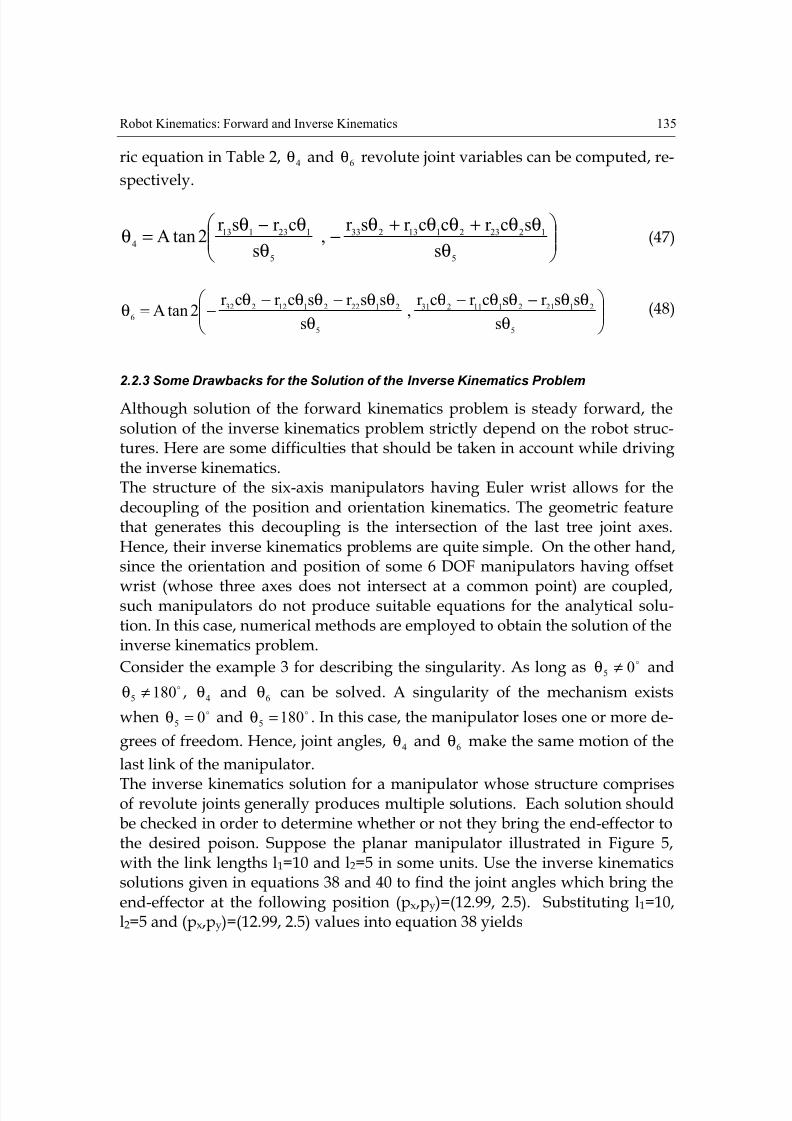
ric equation in Table 2, 4θ and 6θ revolute joint variables can be computed, re-
spectively.
⎟⎟ ⎠
⎞⎜⎜⎝
⎛
θ
θθ+θθ+θ−
θ
θ−θ=θ
5
12232113233
5
123113
4s
scr ccr sr ,
s
cr sr 2tanA (47)
⎟⎟ ⎠
⎞⎜⎜⎝
⎛
θ
θθ−θθ−θ
θ
θθ−θθ−θ−=θ
5
21212111231
5
21222112232
6s
ssr scr cr ,
s
ssr scr cr 2tanA (48)
2.2.3 Some Drawbacks for the Solution of the Inverse Kinematics Problem
Although solution of the forward kinematics problem is steady forward, thesolution of the inverse kinematics problem strictly depend on the robot struc-tures. Here are some difficulties that should be taken in account while drivingthe inverse kinematics.The structure of the six-axis manipulators having Euler wrist allows for thedecoupling of the position and orientation kinematics. The geometric featurethat generates this decoupling is the intersection of the last tree joint axes.Hence, their inverse kinematics problems are quite simple. On the other hand,since the orientation and position of some 6 DOF manipulators having offset
wrist (whose three axes does not intersect at a common point) are coupled,such manipulators do not produce suitable equations for the analytical solu-tion. In this case, numerical methods are employed to obtain the solution of theinverse kinematics problem.
Consider the example 3 for describing the singularity. As long as o05 ≠θ ando1805 ≠θ , 4θ and 6θ can be solved. A singularity of the mechanism exists
when o05 =θ and o1805 =θ . In this case, the manipulator loses one or more de-
grees of freedom. Hence, joint angles, 4θ and 6θ make the same motion of the
last link of the manipulator.
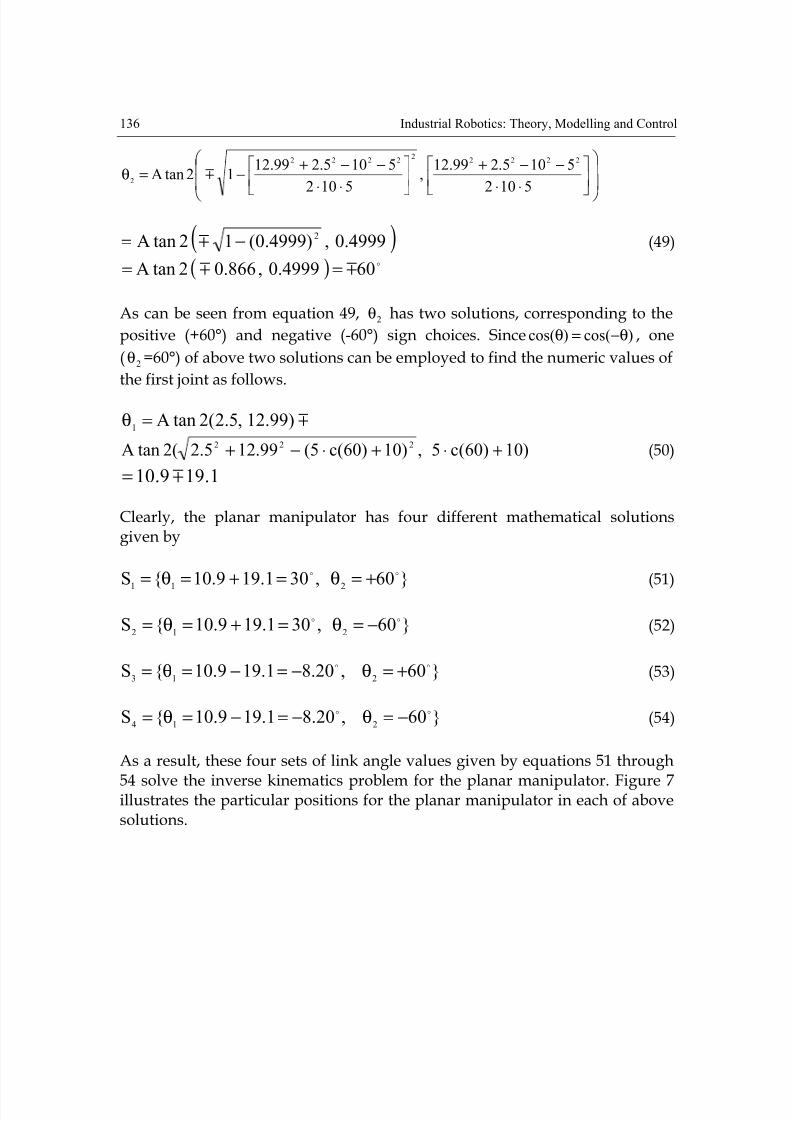
The inverse kinematics solution for a manipulator whose structure comprisesof revolute joints generally produces multiple solutions. Each solution shouldbe checked in order to determine whether or not they bring the end-effector tothe desired poison. Suppose the planar manipulator illustrated in Figure 5,with the link lengths l1=10 and l2=5 in some units. Use the inverse kinematicssolutions given in equations 38 and 40 to find the joint angles which bring theend-effector at the following position (px,py)=(12.99, 2.5). Substituting l1=10,l2=5 and (px,py)=(12.99, 2.5) values into equation 38 yields
8/2/2019 InTech-Robot Kinematics Forward and Inverse Kinematics
http://slidepdf.com/reader/full/intech-robot-kinematics-forward-and-inverse-kinematics 20/32
136 Industrial Robotics: Theory, Modelling and Control
⎟⎟
⎠
⎞
⎜⎜
⎝
⎛
⎥⎦
⎤⎢⎣
⎡
⋅⋅
−−+
⎥⎦
⎤⎢⎣
⎡
⋅⋅
−−+−=θ
5102
5105.299.12,
5102
5105.299.1212tanA
22222
2222
2m
( )4999.0,)4999.0(12tanA 2−= m (49)
( ) o
mm 604999.0,866.02tanA ==
As can be seen from equation 49, 2θ has two solutions, corresponding to the
positive (+60°) and negative (-60°) sign choices. Since )cos()cos( θ−=θ , one
( 2θ =60°) of above two solutions can be employed to find the numeric values of
the first joint as follows.
m)99.12,5.2(2tanA1=θ
)10)60(c5,)10)60(c5(99.125.2(2tanA 222+⋅+⋅−+ (50)
1.199.10 m=
Clearly, the planar manipulator has four different mathematical solutionsgiven by
}60,301.199.10{S211
oo
+=θ=+=θ= (51)
}60,301.199.10{S212
oo
−=θ=+=θ= (52)
}60,20.81.199.10{S213
oo
+=θ−=−=θ= (53)
}60,20.81.199.10{S214
oo
−=θ−=−=θ= (54)
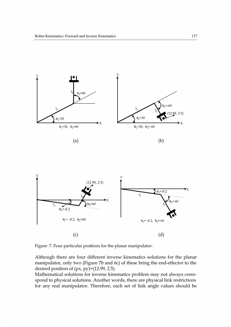
As a result, these four sets of link angle values given by equations 51 through
54 solve the inverse kinematics problem for the planar manipulator. Figure 7illustrates the particular positions for the planar manipulator in each of abovesolutions.
8/2/2019 InTech-Robot Kinematics Forward and Inverse Kinematics
http://slidepdf.com/reader/full/intech-robot-kinematics-forward-and-inverse-kinematics 21/32
Robot Kinematics: Forward and Inverse Kinematics 137
θ1=30
θ2=60
Y
X
l1
l2
θ1=30, θ2=60
(12.99, 2.5)θ1=30
θ2=-60
Y
X
l1 l2
θ1=30, θ2=-60
(a) (b)
(12.99, 2.5)
θ1=-8.2
θ2=60
Y
Xl1
l2
θ1= -8.2, θ2=60
θ1=-8.2
θ2=-60
Y
X
l1
l2
θ1= -8.2, θ2=-60
(c) (d)
Figure 7. Four particular positions for the planar manipulator.
Although there are four different inverse kinematics solutions for the planarmanipulator, only two (Figure 7b and 6c) of these bring the end-effector to thedesired position of (px, py)=(12.99, 2.5).Mathematical solutions for inverse kinematics problem may not always corre-spond to physical solutions. Another words, there are physical link restrictions
for any real manipulator. Therefore, each set of link angle values should be
8/2/2019 InTech-Robot Kinematics Forward and Inverse Kinematics
http://slidepdf.com/reader/full/intech-robot-kinematics-forward-and-inverse-kinematics 22/32
138 Industrial Robotics: Theory, Modelling and Control
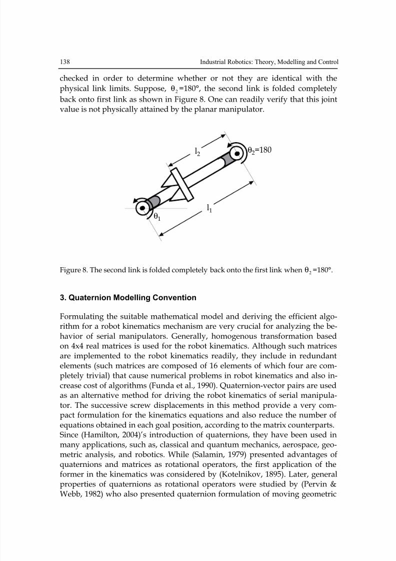
checked in order to determine whether or not they are identical with the
physical link limits. Suppose, 2θ =180°, the second link is folded completely
back onto first link as shown in Figure 8. One can readily verify that this jointvalue is not physically attained by the planar manipulator.
θ2=180
θ1
l2
l1
Figure 8. The second link is folded completely back onto the first link when 2θ =180°.
3. Quaternion Modelling Convention
Formulating the suitable mathematical model and deriving the efficient algo-rithm for a robot kinematics mechanism are very crucial for analyzing the be-havior of serial manipulators. Generally, homogenous transformation basedon 4x4 real matrices is used for the robot kinematics. Although such matricesare implemented to the robot kinematics readily, they include in redundantelements (such matrices are composed of 16 elements of which four are com-pletely trivial) that cause numerical problems in robot kinematics and also in-crease cost of algorithms (Funda et al., 1990). Quaternion-vector pairs are used
as an alternative method for driving the robot kinematics of serial manipula-tor. The successive screw displacements in this method provide a very com-pact formulation for the kinematics equations and also reduce the number ofequations obtained in each goal position, according to the matrix counterparts.Since (Hamilton, 2004)’s introduction of quaternions, they have been used inmany applications, such as, classical and quantum mechanics, aerospace, geo-metric analysis, and robotics. While (Salamin, 1979) presented advantages ofquaternions and matrices as rotational operators, the first application of theformer in the kinematics was considered by (Kotelnikov, 1895). Later, generalproperties of quaternions as rotational operators were studied by (Pervin &
Webb, 1982) who also presented quaternion formulation of moving geometric
8/2/2019 InTech-Robot Kinematics Forward and Inverse Kinematics
http://slidepdf.com/reader/full/intech-robot-kinematics-forward-and-inverse-kinematics 23/32
Robot Kinematics: Forward and Inverse Kinematics 139
objects. (Gu & Luh, 1987) used quaternions for computing the Jacobians for ro-bot kinematics and dynamics. (Funda et al., 1990) compared quaternions with
homogenous transforms in terms of computational efficiency. (Kim & Kumar,1990) used quaternions for the solution of direct and inverse kinematics of a 6-DOF manipulator. (Caccavale & Siciliano, 2001) used quaternions for kine-matic control of a redundant space manipulator mounted on a free-floatingspace-craft. (Rueda et al., 2002) presented a new technique for the robot cali-bration based on the quaternion-vector pairs.
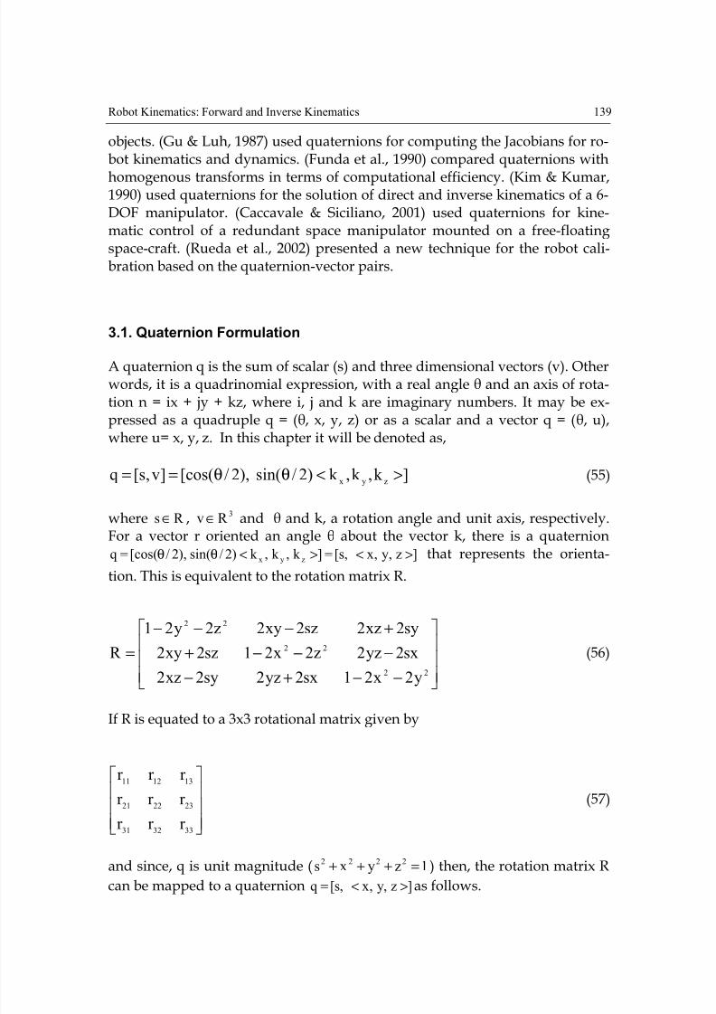
3.1. Quaternion Formulation
A quaternion q is the sum of scalar (s) and three dimensional vectors (v). Otherwords, it is a quadrinomial expression, with a real angle θ and an axis of rota-tion n = ix + jy + kz, where i, j and k are imaginary numbers. It may be ex-pressed as a quadruple q = (θ, x, y, z) or as a scalar and a vector q = (θ, u),where u= x, y, z. In this chapter it will be denoted as,
]k ,k ,k )2/sin(),2/[cos(]v,s[qzyx><θθ== (55)
where R s∈ , 3R v∈ and θ and k, a rotation angle and unit axis, respectively.
For a vector r oriented an angle θ about the vector k, there is a quaternion]z,y,x,s[]k ,k ,k )2/sin(),2/[cos(q zyx ><=><θθ= that represents the orienta-
tion. This is equivalent to the rotation matrix R.
⎥⎥⎥
⎦
⎤
⎢⎢⎢
⎣
⎡
−−+−
−−−+
+−−−
=
22
22
22
y2x21sx2yz2sy2xz2
sx2yz2z2x21sz2xy2
sy2xz2sz2xy2z2y21
R (56)
If R is equated to a 3x3 rotational matrix given by
⎥⎥⎥
⎦
⎤
⎢⎢⎢
⎣
⎡
333231
232221
131211
r r r
r r r
r r r
(57)
and since, q is unit magnitude ( 1zyxs2222=+++ ) then, the rotation matrix R
can be mapped to a quaternion ]z,y,x,s[q ><= as follows.
8/2/2019 InTech-Robot Kinematics Forward and Inverse Kinematics
http://slidepdf.com/reader/full/intech-robot-kinematics-forward-and-inverse-kinematics 24/32
140 Industrial Robotics: Theory, Modelling and Control
2
1r r r
s332211+++
= (58)
s4
r r x 2332
−= (59)
s4
r r y 3113
−= (60)
s4
r r z 1221
−= (61)
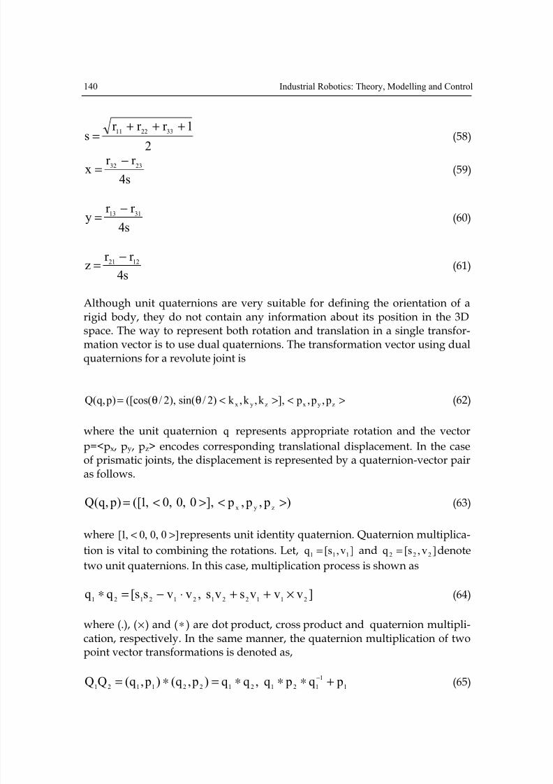
Although unit quaternions are very suitable for defining the orientation of arigid body, they do not contain any information about its position in the 3Dspace. The way to represent both rotation and translation in a single transfor-mation vector is to use dual quaternions. The transformation vector using dualquaternions for a revolute joint is
><><θθ= zyxzyx p, p, p],k ,k ,k )2/sin(),2/([cos() p,q(Q (62)
where the unit quaternion q represents appropriate rotation and the vector
p=<px, py, pz> encodes corresponding translational displacement. In the caseof prismatic joints, the displacement is represented by a quaternion-vector pairas follows.
) p, p, p],0,0,0,1([) p,q(Qzyx><><= (63)
where ]0,0,0,1[ >< represents unit identity quaternion. Quaternion multiplica-
tion is vital to combining the rotations. Let, ]v,s[q 111 = and ]v,s[q 222 = denotetwo unit quaternions. In this case, multiplication process is shown as
]vvvsvs,vvss[qq211221212121
×++⋅−=∗ (64)
where (.), (× ) and (∗ ) are dot product, cross product and quaternion multipli-cation, respectively. In the same manner, the quaternion multiplication of twopoint vector transformations is denoted as,
1
1
12121221121 pq pq,qq) p,q() p,q(QQ+∗∗∗=∗=
−
(65)
8/2/2019 InTech-Robot Kinematics Forward and Inverse Kinematics
http://slidepdf.com/reader/full/intech-robot-kinematics-forward-and-inverse-kinematics 25/32
Robot Kinematics: Forward and Inverse Kinematics 141
where, ). pv(v2) pv(s2 pq pq 2112112
1
121 ××+×+=∗∗− A unit quaternion inverse
requires only negating its vector part, i.e.
]v,s[]v,s[q 1−==
− (66)
Finally, an equivalent expression for the inverse of a quaternion-vector paircan be written as,
)q* p*q,q(Q 111 −−−−= (67)
where ))]. p(v(v2)) p(v(s2[ pq* p*q1
−××+−×−+−=−−
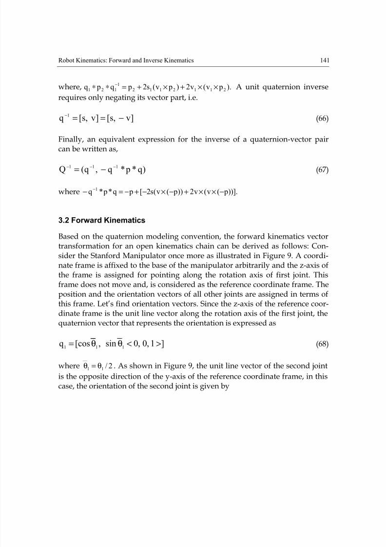
3.2 Forward Kinematics
Based on the quaternion modeling convention, the forward kinematics vectortransformation for an open kinematics chain can be derived as follows: Con-sider the Stanford Manipulator once more as illustrated in Figure 9. A coordi-nate frame is affixed to the base of the manipulator arbitrarily and the z-axis ofthe frame is assigned for pointing along the rotation axis of first joint. This
frame does not move and, is considered as the reference coordinate frame. Theposition and the orientation vectors of all other joints are assigned in terms ofthis frame. Let’s find orientation vectors. Since the z-axis of the reference coor-dinate frame is the unit line vector along the rotation axis of the first joint, thequaternion vector that represents the orientation is expressed as
]1,0,0sin,[cosq111
><θθ= (68)
where 2/11 θ=θ . As shown in Figure 9, the unit line vector of the second joint
is the opposite direction of the y-axis of the reference coordinate frame, in this
case, the orientation of the second joint is given by
8/2/2019 InTech-Robot Kinematics Forward and Inverse Kinematics
http://slidepdf.com/reader/full/intech-robot-kinematics-forward-and-inverse-kinematics 26/32
142 Industrial Robotics: Theory, Modelling and Control
z 0,1
h1
d2
d3
Unit line vector
of the first joint
Z
θ1
θ2
X
Y
θ4,θ6
θ5
Figure 9. The coordinate frame and unit line vectors for the Stanford Manipulator.
]0,1,0sin,[cosq222
>−<θθ= (69)
Because, the third joint is prismatic; there is only a unit identity quaternionthat can be denoted as
]0,0,0,1[q3
><= (70)
Orientations of the last three joints are determined as follows using the sameapproach described above.
]1,0,0sin,[cosq444
><θθ= (71)
]0,1,0sin,[cosq 555><θθ=
(72)
]1,0,0sin,[cosq666
><θθ= (73)
The position vectors are assigned in terms of reference coordinate frame as fol-lows. When the first joint is rotated anticlockwise direction around the z axis
of reference coordinate frame by an angle of 1θ , the link d2 traces a circle in the
xy-plane which is parallel to the xy plane of the reference coordinate frame asgiven in Figure 10a. Any point on the circle can be determined using the vector
8/2/2019 InTech-Robot Kinematics Forward and Inverse Kinematics
http://slidepdf.com/reader/full/intech-robot-kinematics-forward-and-inverse-kinematics 27/32
Robot Kinematics: Forward and Inverse Kinematics 143
>θ−θ>=<<=112121z1y1x1
h,cosd,sind p, p, p p (74)
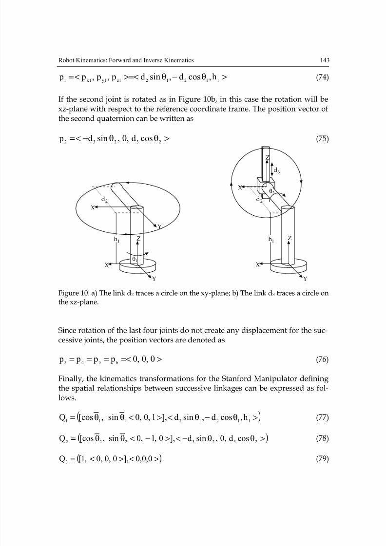
If the second joint is rotated as in Figure 10b, in this case the rotation will bexz-plane with respect to the reference coordinate frame. The position vector ofthe second quaternion can be written as
>θθ−<=23232
cosd,0,sind p (75)
z 0,1
h1
d2
θ1
X
Y
Z
X
Y
z 0,1
h1
d2
d3
Z
θ2
X
Y
Z
X
Figure 10. a) The link d2 traces a circle on the xy-plane; b) The link d3 traces a circle onthe xz-plane.
Since rotation of the last four joints do not create any displacement for the suc-cessive joints, the position vectors are denoted as
>=<=== 0,0,0 p p p p6543
(76)
Finally, the kinematics transformations for the Stanford Manipulator definingthe spatial relationships between successive linkages can be expressed as fol-lows.
( )>θ−θ<><θθ=11212111
h,cosd,sind],1,0,0sin,[cosQ (77)
( )>θθ−<>−<θθ=2323222
cosd,0,sind],0,1,0sin,[cosQ (78)
( )><><= 0,0,0],0,0,0,1[Q3
(79)
8/2/2019 InTech-Robot Kinematics Forward and Inverse Kinematics
http://slidepdf.com/reader/full/intech-robot-kinematics-forward-and-inverse-kinematics 28/32
144 Industrial Robotics: Theory, Modelling and Control
( )><><θθ= 0,0,0],1,0,0sin,[cosQ 444 (80)
( )><><θθ= 0,0,0],0,1,0sin,[cosQ 555 (81)
( )><><θθ= 0,0,0],1,0,0sin,[cosQ666
(82)
The forward kinematics of the Stanford Manipulator can be determined in the
form of equation 62, multiplying all of the iQ matrices, where i=1,2, …, 6.
[ ]( )>θ+θθ−θ−θθ−θ<=2312131221312
cdh,ssdcd,scdsd,v,s) p,q(Q (83)
where 11Ms=
and M,M,Mv 141312>=<
are given by equation 98.
3.3 Inverse Kinematics
To solve the inverse kinematics problem, the transformation quaternion is de-fined as
) p, p, p],c, b,a,w([]T,R [zyxww><><= (84)
where )T,R ( ww represents the known orientation and translation of the robotend-effector with respect to the base. Let iQ )6i1( ≤≤ denotes kinematics trans-
formations describing the spatial relationships between successive coordinate
frames along the manipulator linkages such as ) p,q(Q 111 = , ) p,q(Q 222 = …
) p,q(Q 666 = .
The quaternion vector products iM and the quaternion vector pairs 1 j N+
are
defined as
1iii
MQM+
= (85)
i
1
i1i NQ N
−
+= (86)
where 5i1 ≤≤ . Note that 66 QM = and ]T,R [ N ww1 = . In order to extract joint
variables as functions of s, v, px, py, pz and fixed link parameters, appropriate
iM and 1 j N+
terms are equated, such as , NM 11 = 22 NM = … 66 NM = . For the
reason of compactness, 2/iθ , )2/sin( iθ , )2/cos( iθ , )sin( iθ and )cos( iθ will be
represented as iθ , is , ic , is and ic respectively. The link transformation matri-
ces were formerly developed. The inverse transformations can be written as
follows using equation 67.
8/2/2019 InTech-Robot Kinematics Forward and Inverse Kinematics
http://slidepdf.com/reader/full/intech-robot-kinematics-forward-and-inverse-kinematics 29/32
Robot Kinematics: Forward and Inverse Kinematics 145
)h,d,0],1,0,0s,c([Q1211
1
1>−−<><−=
− (87)
)d,0,0],0,1,0s,c([Q322
1
2>−<><=
− (88)
)0,0,0],0,0,0,1([Q 1
3><><=
−(89)
)0,0,0],1,0,0s,c([Q44
1
4><><−=
− (90)
)0,0,0],0,1,0s,c([Q 55
1
5 ><><−=−
(91)
)0,0,0],1,0,0s,c([Q 661
6 ><><−=− (92)
The quaternion vector products are
( )><><θθ== 0,0,0],1,0,0s,c[QM6666
(93)
)0,0,0],sc,cs,ss,cc([MQM65656565655
><><== (94)
)0,0,0],M,M,M,M([MQM44434241544
><><== (95)
where,
)64(541 ccM+
= ,
)64(542 ssM−
−= ,
)64(543 csM−
= and
)46(544 scM+
= .
)0,0,0],M,M,M,M([MQM34333231433
><><== (96)
where,
4232 MM = ,
4333 MM = and
4434 MM = .
)cd,0,sd],M,M,M,M([MQM232324232221322>−<><== (97)
where,
8/2/2019 InTech-Robot Kinematics Forward and Inverse Kinematics
http://slidepdf.com/reader/full/intech-robot-kinematics-forward-and-inverse-kinematics 30/32
146 Industrial Robotics: Theory, Modelling and Control
43241221 MsMcM −= ,
44242222 MsMcM −= , 41243223 MsMcM −= and
42244224 MsMcM += .
)M,M,M],M,M,M,M([MQM 17161514131211211 ><><== (98)
where,
)MsMc(sMcM 422442121111 −−= ,
23122112 MsMcM −= ,
22123113 MsMcM += ,
24121114 McMsM+=
,2131215 scdsdM θθ−θ= ,
2131216 ssdcdM θθ−θ−= and
23117 cdhM θ+= .
The quaternion vector pairs are
) p, p, p]c, b,a,w([ Nzyx1><><= (99)
)h p, N, N], N, N, N, N([ NQ N 1z2625242322211
1
12>−<><==
−
(100)
where,
1121 sccw N += ,
1122 s bca N += ,
1123 sac b N −= ,
1124 swcc N −= ,
1y1x25 s pc p N += and
21y1x26 dc ps p N −+−= .
) N, N, N], N, N, N, N([ NQ N373635343332312
1
23><><==
− (101)
where,
24221231 Ns Nc N −= ,
23222232 Ns Nc N −= ,
22223233 Ns Nc N += ,
21224234 Ns Nc N += ,
) ph(s)s pc p(c N z121y1x235 −−+= , 21x1y36 ds pc p N −−= ,
31y1x21z237 d)s pc p(s)h p(c N −+−−= .
8/2/2019 InTech-Robot Kinematics Forward and Inverse Kinematics
http://slidepdf.com/reader/full/intech-robot-kinematics-forward-and-inverse-kinematics 31/32
Robot Kinematics: Forward and Inverse Kinematics 147
)0,0,0], N, N, N, N([ NQ N444342413
1
34><><==
− (102)
where, 3141 N N = ,
3242 N N = ,
3343 N N = and
3444 N N = .
The first joint variable 1θ can be determined equating the second terms of M2
and N2 as follows.
)d,d p p(2tanA) p, p(2tanA 22
22
y2
xyx1 −+±−=θ (103)
The joint variables 2θ and 3d are computed equating the first and third ele-
ments of M3 and N3 respectively.
) ph, ps pc(2tanAz1y1x12
−θ+θ±=θ (104)
)h p(c) ps pc(sd1z2y1x123
−θ+θ+θθ−= (105)
2
43
2
42
2
5 N Ns+=
,2
44
2
41
2
5 N Nc+=
, 41
44
64 N
N
)tan(=θ+θ
and 43
42
64 N
N
)tan(−=θ−θ
equations can be derived form equating the terms M4 to N4, where,
41)64(5 Ncc =+
, 42)64(5 Nss =−−
, 43)64(5 Ncs =−
and 44)46(5 Nsc =+
. In this case, the
orientation angles of the Euler wrist can be determined as follows.
( )2
44
2
41
2
43
2
425 N N, N N2arctan ++±=θ (106)
⎟⎟ ⎠
⎞⎜⎜⎝
⎛ −+⎟⎟
⎠
⎞⎜⎜⎝
⎛ =θ
43
42
41
44
4 N
Narctan
N
Narctan (107)
⎟⎟ ⎠
⎞⎜⎜⎝
⎛ −−⎟⎟
⎠
⎞⎜⎜⎝
⎛ =θ
43
42
41
44
6 N
Narctan
N
Narctan (108)
8/2/2019 InTech-Robot Kinematics Forward and Inverse Kinematics
http://slidepdf.com/reader/full/intech-robot-kinematics-forward-and-inverse-kinematics 32/32
148 Industrial Robotics: Theory, Modelling and Control
4. References
Denavit, J. & Hartenberg, R. S. (1955). A kinematic notation for lower-pairmechanisms based on matrices. Journal of Applied Mechanics, Vol., 1(June 1955) pp. 215-221
Funda, J.; Taylor, R. H. & Paul, R.P. (1990). On homogeneous transorms, qua-ternions, and computational efficiency. IEEE Trans.Robot. Automat., Vol.,6 (June 1990) pp. 382–388
Kucuk, S. & Bingul, Z. (2004). The Inverse Kinematics Solutions of IndustrialRobot Manipulators, IEEE Conferance on Mechatronics, pp. 274-279, Tur-key, June 2004, Istanbul
Craig, J. J. (1989). Introduction to Robotics Mechanics and Control, USA:Addision-
Wesley Publishing CompanyHamilton, W. R. (1869). Elements of quaternions, Vol., I & II, Newyork ChelseaSalamin, E. (1979). Application of quaternions to computation with rotations. Tech.,
AI Lab, Stanford Univ., 1979Kotelnikov, A. P. (1895). Screw calculus and some of its applications to geometry
and mechanics. Annals of the Imperial University of Kazan.Pervin, E. & Webb, J. A. (1983). Quaternions for computer vision and robotics,
In conference on computer vision and pattern recognition. pp 382-383,Washington, D.C.
Gu, Y.L. & Luh, J. (1987). Dual-number transformation and its application to
robotics. IEEE J. Robot. Automat. Vol., 3, pp. 615-623Kim, J. H. & Kumar, V. R. (1990). Kinematics of robot manipulators via line
transformations. J. Robot. Syst., Vol., 7, No., 4, pp. 649–674Caccavale, F. & Siciliano, B. (2001). Quaternion-based kinematic control of re-
dundant spacecraft/ manipulator systems, In proceedings of the 2001IEEE international conference on robotics and automation, pp. 435-440
Rueda, M. A. P.; Lara, A. L. ; Marinero, J. C. F.; Urrecho, J. D. & Sanchez, J.L.G.(2002). Manipulator kinematic error model in a calibration processthrough quaternion-vector pairs, In proceedings of the 2002 IEEE interna-tional conference on robotics and automation, pp. 135-140


![Inverse Kinematics and Gaze Stabilization for the Rochester ......3 Inverse Kinematics 3.1 Inverse Kinematics: O,A,T from TOOL The mathematics in [Brown and Rimey, 1988] Section 9](https://img.pdfslide.net/doc/110x75/60be15e583990e1ab8600327/inverse-kinematics-and-gaze-stabilization-for-the-rochester-3-inverse-kinematics.jpg)