Inversion of coupled groundwater flow and heat transfer

M. Bücker 1, V.Rath 2 & A. Wolf 1

1 Scientific Computing, 2 Applied Geophysics

Bommerholz 14.8-18.8, Sommerschule 2006: Automatisches Differenzieren

2

x (km)

020

4060

80100y

(km)

0

20

40

60

z(km

)

0

1

2

3

4

z(k

m)

Y

X

Z

Contents

• Geothermal modeling in SHEMAT

• Bayesian inversion method

• Validation of the inversion code

• Analytical solution

• Numerical experiments

• Covariance and Resolution matrices

• Quality Indicator

• Summary

3

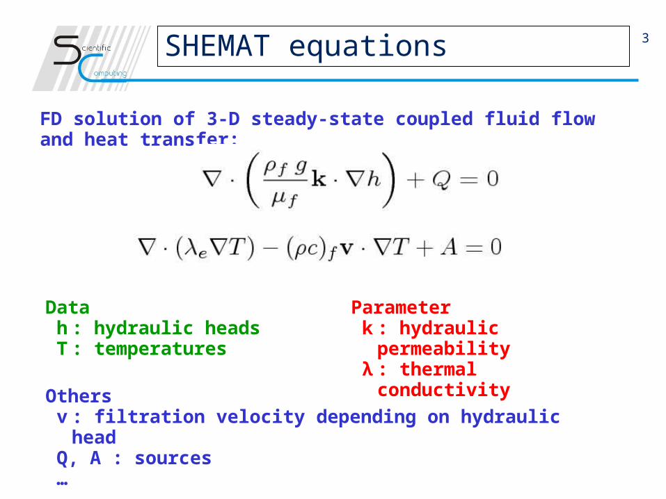
FD solution of 3-D steady-state coupled fluid flow and heat transfer:

SHEMAT equations

Data h : hydraulic heads T : temperatures

Parameter k : hydraulic permeability λ : thermal conductivity

Others v : filtration velocity depending on hydraulic head Q, A : sources …

4SHEMAT intern

• Dirichlet and Neumann boundary conditions

• fluid and rock properties dependent on temperature

and pressure

• nonlinear solution by simple alternating fixed point

iteration

• linear solvers

•direct (from LAPACK) and iterative solvers

(BiCGstab, parallelized with OpenMP )

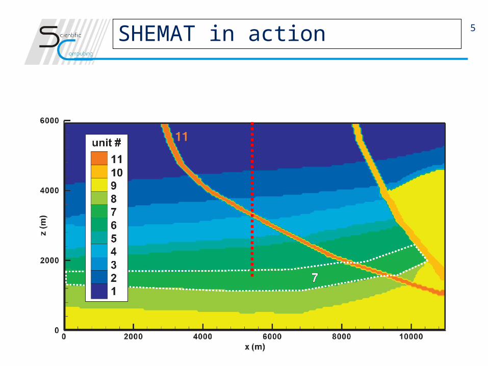
5SHEMAT in action

6

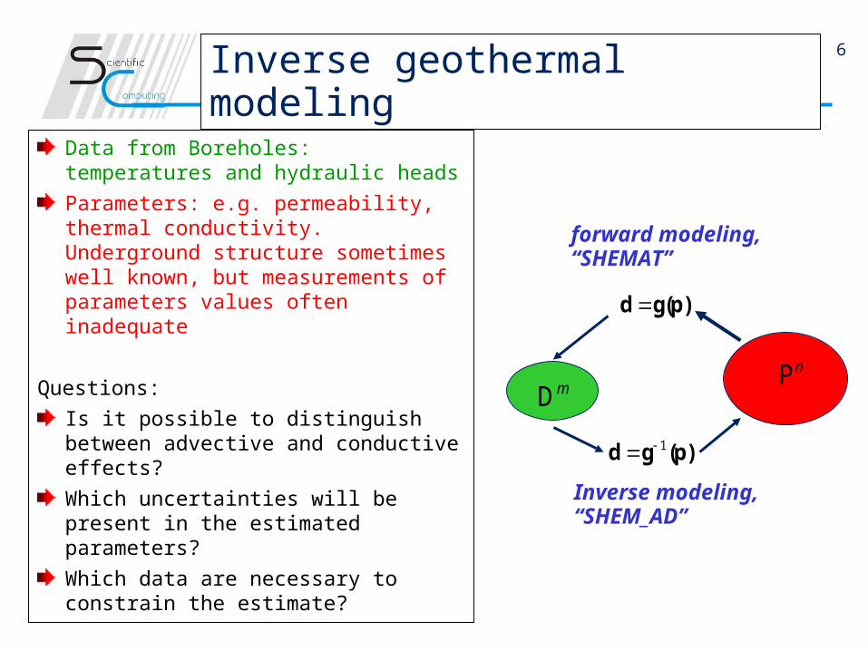
Data from Boreholes: temperatures and hydraulic heads

Parameters: e.g. permeability, thermal conductivity. Underground structure sometimes well known, but measurements of parameters values often inadequate

Questions:

Is it possible to distinguish between advective and conductive effects?

Which uncertainties will be present in the estimated parameters?

Which data are necessary to constrain the estimate?

Inverse geothermal modeling

d g(p)

1d g (p)

nPmD

forward modeling,“SHEMAT”

Inverse modeling,“SHEM_AD”

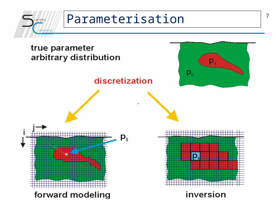
7Parameterisation

8

General assumptions:

• A-priori error bounds of

data and parameters

• Arbitrary integration of

boundary conditions

• No ad-hoc regularisation

parameters

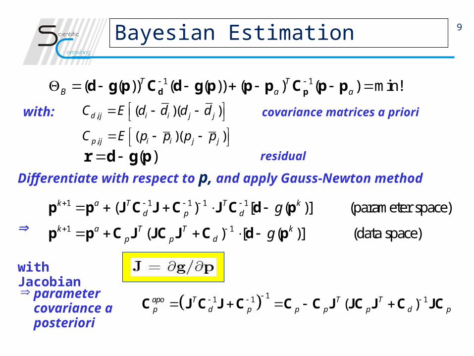
Bayesian Inversion

Thomas Bayes, 1702-1761

9

with: covariance matrices a priori

residual

Differentiate with respect to p, and apply Gauss-Newton method

1 1( ( )) ( ( )) ( ) ( ) min!T TB a a

d pd g p C d g p p p C p p

1 1 1 1 1

1 1

( ) [ ( )] (parameter space)

( ) [ ( )] (data space)

k a T T kd p d

k a T T kp p d

g

g

p p J C J C J C d p

p p C J JC J C d p

,

,

( )( )

( )( )

d ij i i j j

p ij i i j j

C E d d d d

C E p p p p

( ) r d g p

11 1 1( )apo T T Tp d p p p p d p

C J C J C C C J JC J C JC

with Jacobian

parameter covariance a posteriori

Bayesian Estimation

10

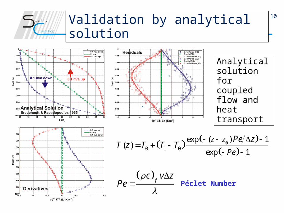
Analytical solution for coupled flow and heat transport

00 1 0

exp ( ) 1

exp 1( )

z z

Pe

Pe zT z T T T

fc v zPe

Péclet Number

Validation by analytical solution

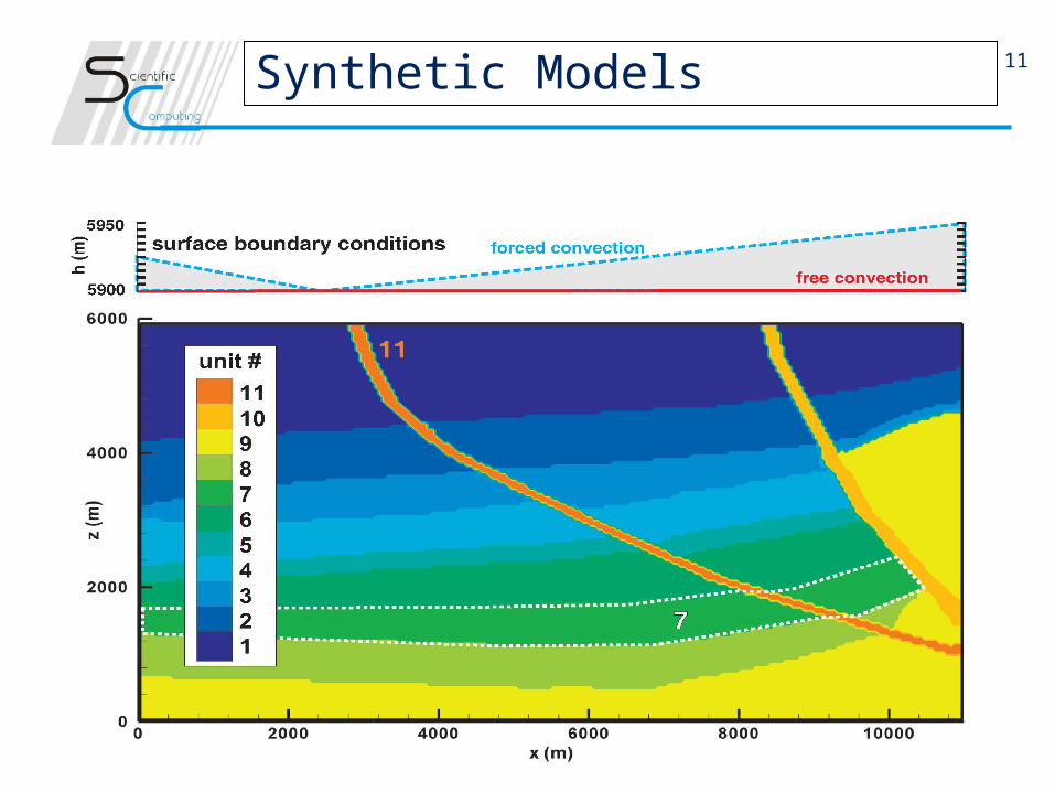
11Synthetic Models

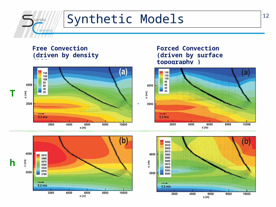
12

Free Convection(driven by density differences)

Forced Convection(driven by surface topography )

Synthetic Models

T

h

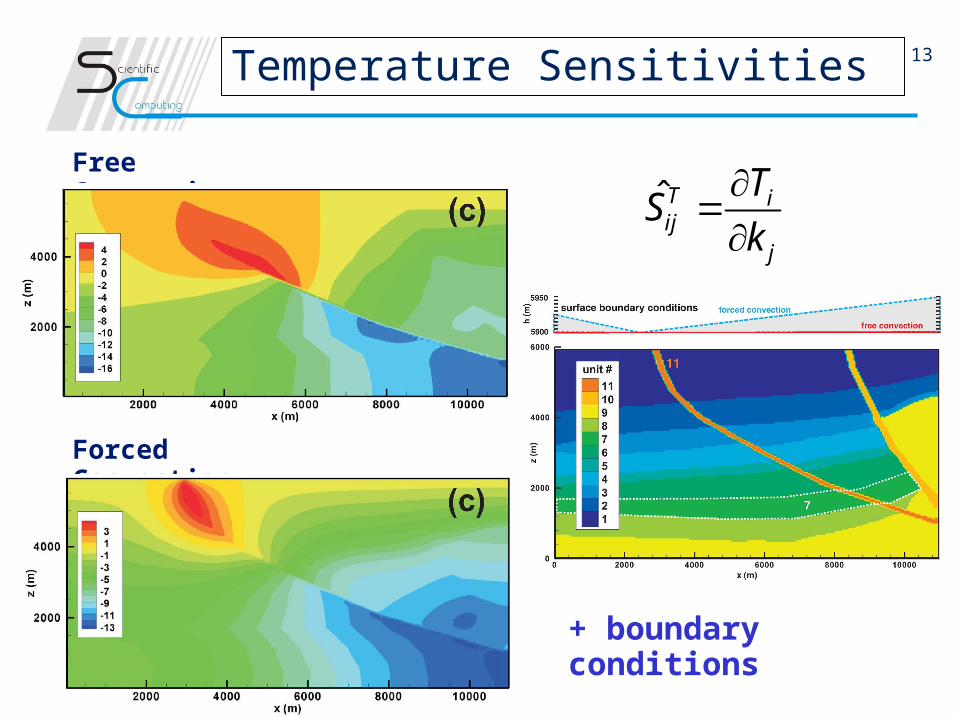
13

Free Convection

Forced Convection

ˆT iij

j

TS

k

Temperature Sensitivities

+ boundary conditions

14

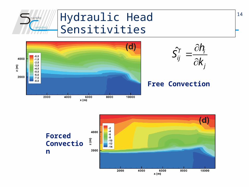
Free Convection

Forced Convection

ˆT iij

j

hS

k

Hydraulic Head Sensitivities

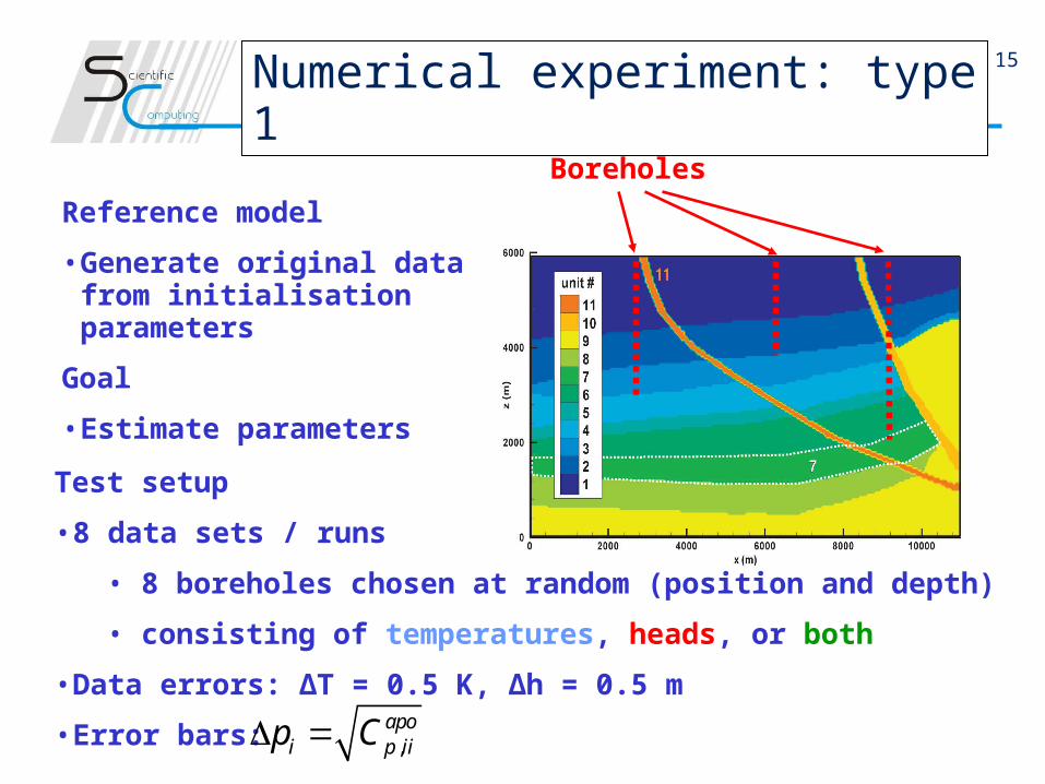
15

Test setup

• 8 data sets / runs

• 8 boreholes chosen at random (position and depth)

• consisting of temperatures, heads, or both

• Data errors: ΔT = 0.5 K, Δh = 0.5 m

• Error bars: ,apo

i p iip C

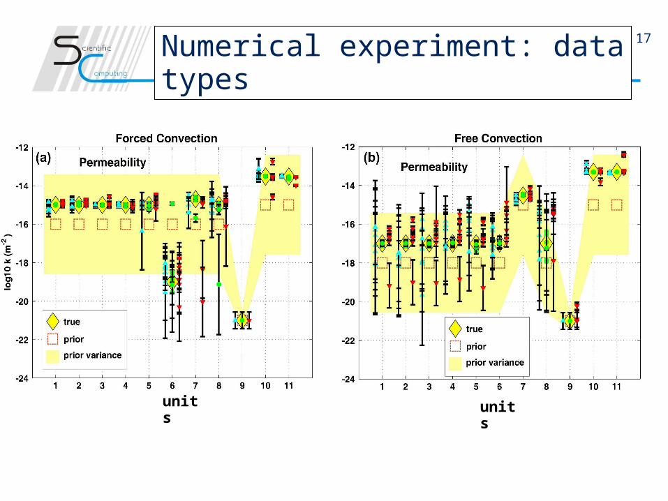
Numerical experiment: type 1

Reference model

• Generate original data from initialisation parameters

Goal

• Estimate parameters

Boreholes

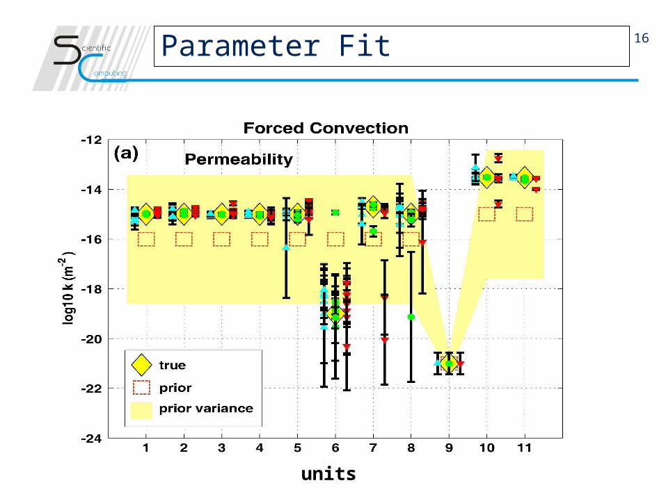
16Parameter Fit

units

17

unitsunits

Numerical experiment: data types

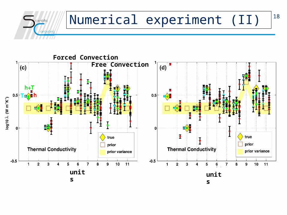
18Numerical experiment (II)

Forced Convection Free Convection

unitsunits

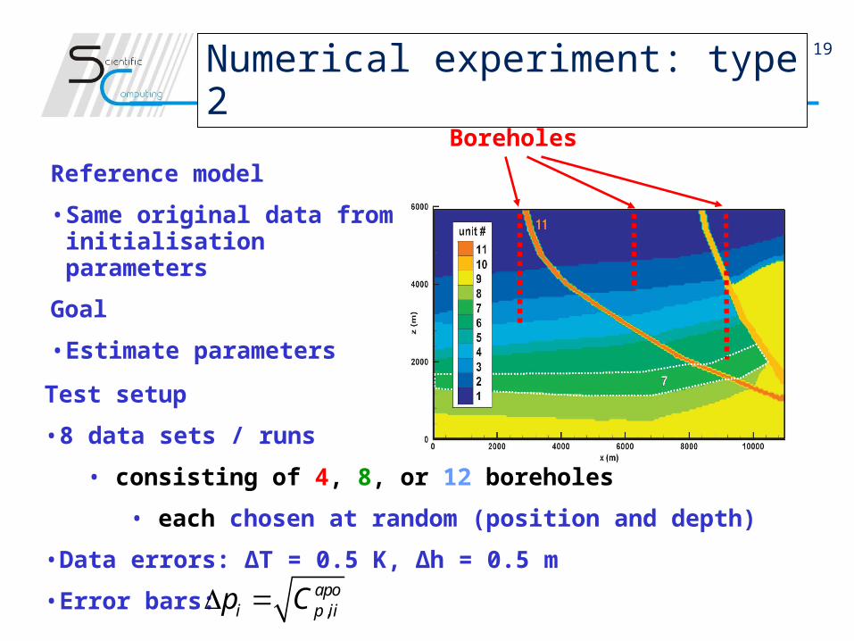
19

Test setup

• 8 data sets / runs

• consisting of 4, 8, or 12 boreholes

• each chosen at random (position and depth)

• Data errors: ΔT = 0.5 K, Δh = 0.5 m

• Error bars: ,apo

i p iip C

Numerical experiment: type 2

Reference model

• Same original data from initialisation parameters

Goal

• Estimate parameters

Boreholes

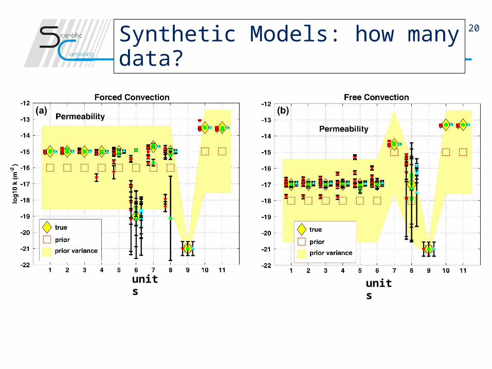
20

unitsunits

Synthetic Models: how many data?

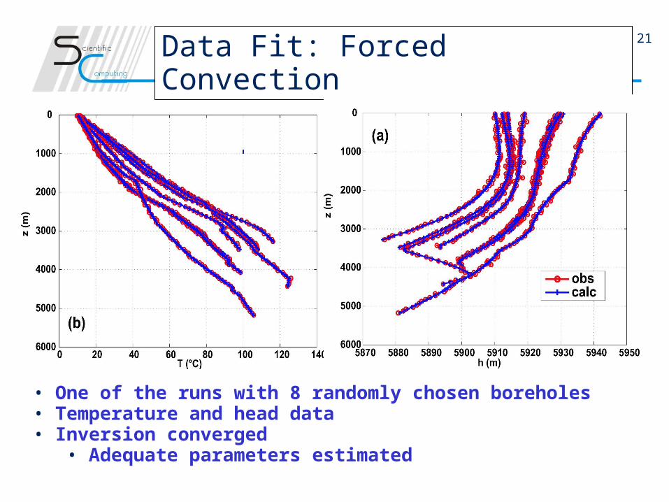
21Data Fit: Forced Convection

• One of the runs with 8 randomly chosen boreholes• Temperature and head data• Inversion converged

• Adequate parameters estimated

22Information Discussion

Questions:

• Which uncertainties will be present in the estimated

parameters?

• Which data are necessary to constrain the estimate?

23

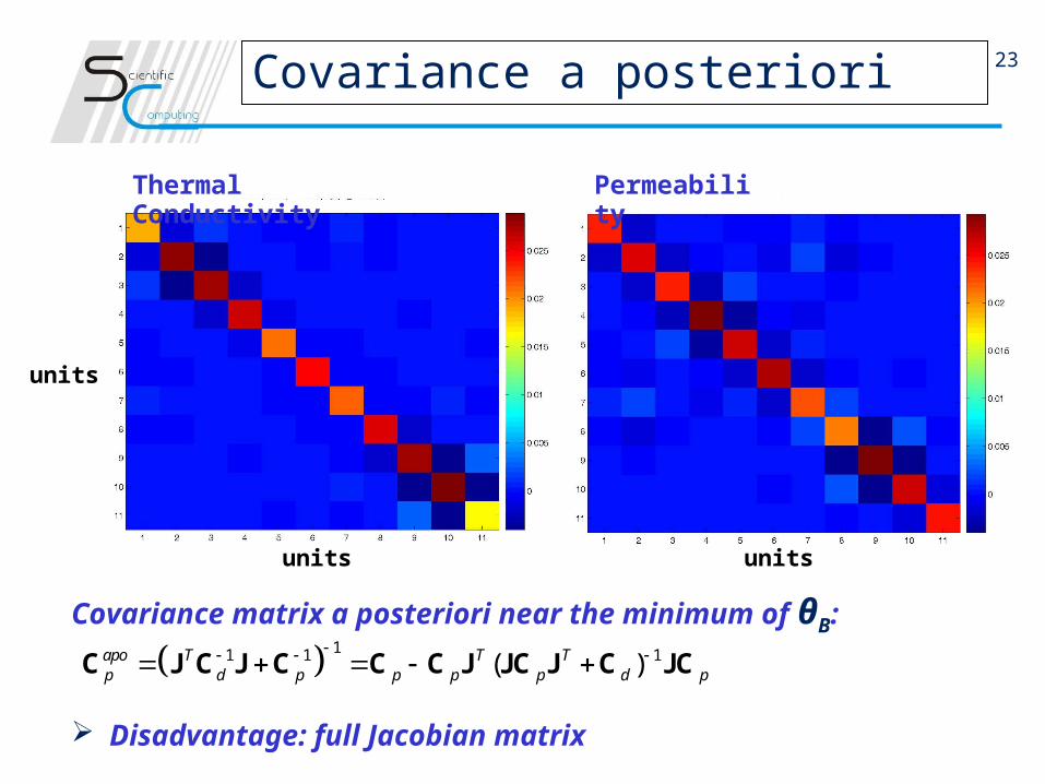
Covariance matrix a posteriori near the minimum of θB:

11 1 1( )apo T T Tp d p p p p d p

C J C J C C C J JC J C JC

Covariance a posteriori

Disadvantage: full Jacobian matrix

units units

units

Thermal Conductivity Permeability

24

,

( )

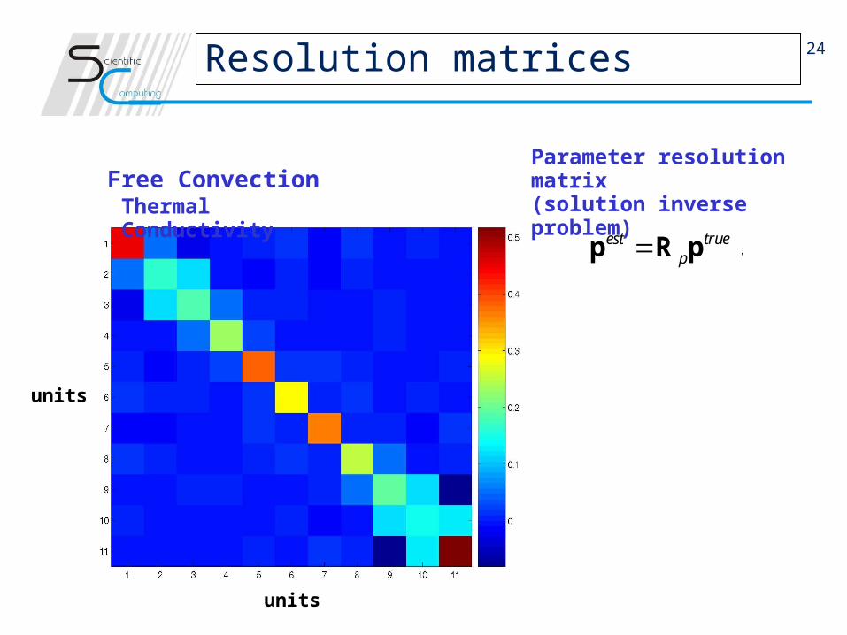
est truep

apo apr Tp p p

p R p

R I -C C

Parameter resolution matrix(solution inverse problem)Free Convection

Thermal Conductivity

Resolution matrices

units

units

25

x (km)

020

4060

80100y

(km)

0

20

40

60

z(km

)

0

1

2

3

4

z(k

m)

Y

X

Z

kz

2E-141.8E-141.6E-141.4E-141.2E-141E-148E-156E-154E-152E-15

x (km)

020

4060

80100y

(km)

0

20

40

60

z(km

)

0

1

2

3

4

z(k

m)

Y

X

Z

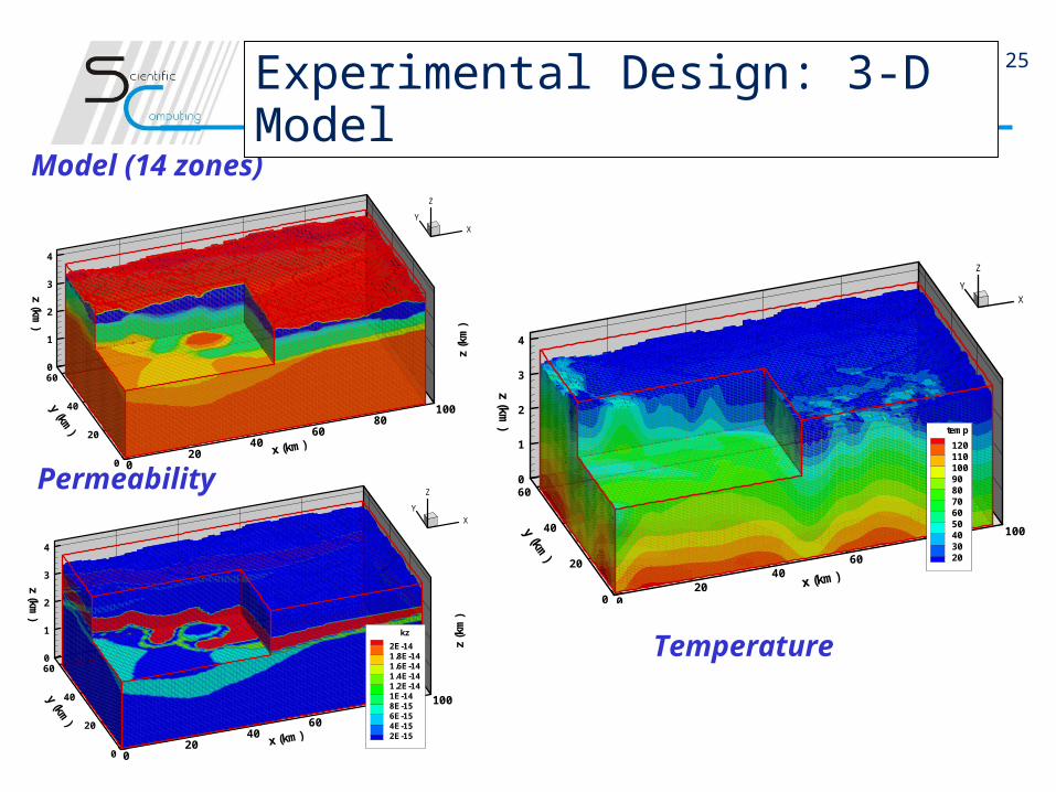
Permeability

Model (14 zones)

x (km)

020

4060

80100y

(km)

0

20

40

60

z(km

)

0

1

2

3

4

Y

X

Z

temp

1201101009080706050403020

Temperature

Experimental Design: 3-D Model

26

x (m)

y (

m)

TEMP method: t2

0 2 4 6 8

x 104

0

1

2

3

4

5

x 104

5

10

15

20

25

30

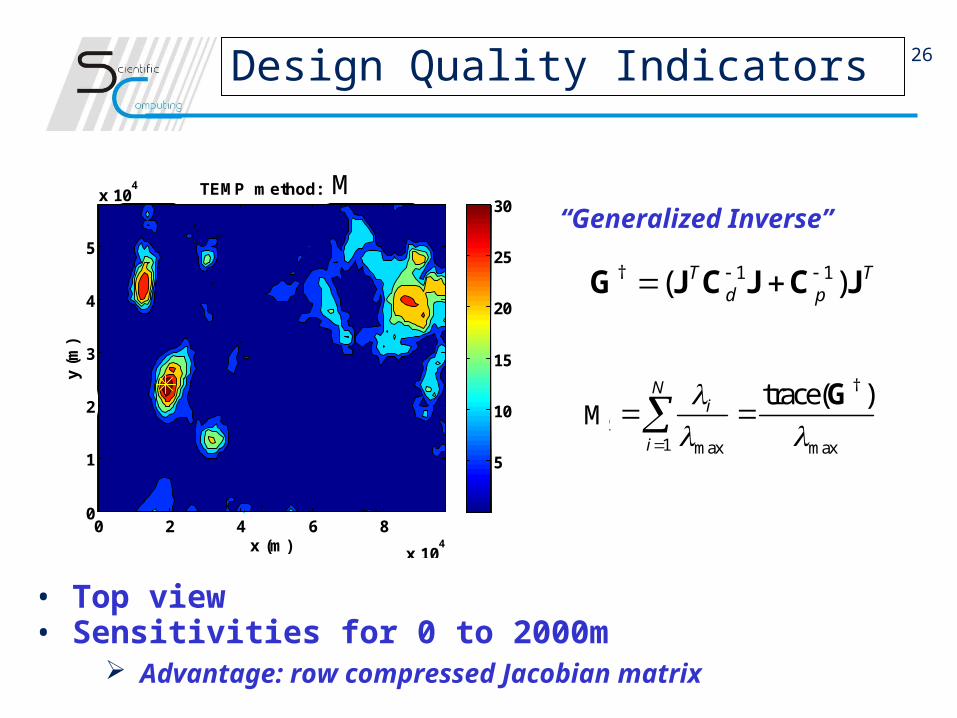
Design Quality Indicators

• Top view• Sensitivities for 0 to 2000m

† 1 1

†

( )T Td p

G J C J C J

UΛV G

“Generalized Inverse”

†

21 max max

†3

1

trace( )

det( )

...

Ni

i

N

ii

t

t

G

G

M

M

Advantage: row compressed Jacobian matrix

27

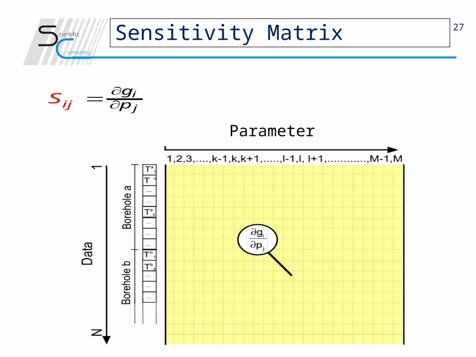
Parameter

ijijgpS

Sensitivity Matrix

28

• Successful validation without data from real experiments, which can be expensive

• Covariance and Resolution matrices can help to decide which parameters needs to be determent more exactly– But their computation may be expensive

Future work:• Reverse-Mode AD version make it possible to use

algorithms with:– improved convergency (matrix free Newton-Krylow)– smaller memory requirements for larger models

• Validation with real experimental data

Summary and Conclusions

29The End

THANK YOU

FOR YOUR ATTENTION !