Inversion of Well Logs Into Facies Accountingfor Spatial Dependencies and Convolution

Effects

David V. Lindberg, Norwegian University of Science and Technology, Eivind Rimstad,Statoil ASA and Henning Omre, Norwegian University of Science and Technology

Summary

We predict facies from wireline well log data for a fluvial deposit system offshore Norway. The

wireline well logs used are sonic, gamma ray, neutron porosity, bulk density and resistivity.

We solve this inverse problem in a predictive Bayesian setting, and perform the associated

model parameter estimation. Spatial vertical structure of the facies is included in the model

by a Markov chain assumption, making geological model interpretation possible. We also

take convolution effect into account, assuming that the observed logs might be measured

as a weighted sum of properties over a facies interval. We apply the methods on real well

data, with thick facies layers inferred from core samples. The proposed facies classification

model is compared to a naive Bayesian classifier, which do not take into account neither

vertical spatial dependency, dependencies between the wireline well logs nor convolution

effect. Results from a blind well indicate that facies predictions from our model are more

reliable than predictions from the naive model in terms of correct facies classification and

predicted layer thickness.

Introduction

Determination of categorical attributes like facies or lithofacies throughout a well is usually

performed by qualitative well log and core sample analysis, developed from geological ex-

perience and rock physics models. This classification is of importance in exploration and

1

development of petroleum reservoirs. Continuous wireline logs are collected in most wells

and contain quantitative information, but because of noise and possible convolution they

may have limited information of the true rock properties. Because reservoir properties are

directly measured on core samples, it is typically the most reliable petrophysical data, but

are only available in low number of cored wells for many fields as coring introduces additional

cost and risk during drilling. Where available, the core plugs are usually sampled discretely

throughout the well, moreover they may be preferentially sampled. In some locations along

the well it may not be possible to extract core plugs resulting from fractures and poorly

consolidated plugs, while other locations may be overrepresented caused by easier sampling.

Thus, both the geologist and the petrophysicist need to use petrophysical logs for facies

recognition and well evaluation, but because of convolution effects in the logging measure-

ment, facies recognition may be challenging and data evaluation inaccurate. An inversion of

the petrophysical logs may therefore be valuable both for geologist and petrophysicist. In

this paper, we study facies along a vertical 1D-profile through the subsurface layers. The

objective is to create a model for prediction of the subsurface layers based on the observed

wireline well logs. This is an ill-posed inverse problem, as multiple facies combinations may

return the same observed well logs because of various noise components.

Several classification methods for facies and lithofacies determination from multiple logs

are presented in the literature. The two main classification approaches are based on ar-

tificial intelligence and multivariate statistical methods. Artificial intelligence methods in-

clude artificial neural networks (Qi and Carr , 2006; Tang et al. , 2011), and fuzzy logic

(Chang et al. , 1997; Cuddy , 2000). Multivariate statistical classification methods include

discriminant and cluster analysis, regression analysis (Guo et al. , 2007; Tang and White ,

2008), statistical tree-based analysis (Perez et al. , 2005), and Bayesian analysis. In this

study we focus on Bayesian classifiers.

2

By approaching the problem in a Bayesian setting, we are able to incorporate in the model

a priori knowledge along with the information carried by the well log data. General geological

knowledge, derived from geological exploration of the facies in the reservoir, is captured in

the prior model. The forward function, defining the petrophysical well log measures given

the facies, is specified as a likelihood model. The prior and the likelihood models define the

posterior model representing the facies distribution along the well, given the observations. In

Loures and Moraes (2006), porosity and clay volume is predicted in a Bayesian framework

based on rock physics likelihood models, which again is used to classify facies by a simple

cut-off model. In Coudert et al. (1994) and Li and Anderson-Sprecher (2006), a Bayesian

classification method is described in which the well logs are assumed to be independent, the

likelihood models are estimated by Gaussian distributions and the prior model is defined as

the lithofacies proportions in the well. Li and Anderson-Sprecher (2006) terms this approach

a naive Bayesian (NB) classifier, which is found to be superior to linear discriminant analysis,

and a Gaussian likelihood model outperforms non-parametric kernel density models. A

similar classifier by use of beta likelihood models is described in Tang and Ji (2006) and

Tang and White (2008), and this model appears to perform better than probabilistic neural

networks, linear discriminant analysis and multinomial logistic regression. Consequently,

Bayesian inversion seems to be well suited for facies classification from well log data.

Most facies classification methods found in the literature assume that the well logs are

vertically elementwise independent. To take spatial dependency into account the predictions

are sometimes post-processed, see for example Qi and Carr (2006) in which predicted thin

lithofacies layers are removed to avoid small-scale alterations. In the current study, we include

spatial dependency by choosing a prior facies model according to Eidsvik et al. (2004). The

underlying spatial coupling is captured with a Markov chain assumption in the prior facies

model, in which each element in the well conditioned on the rest of the well is dependent

3

on its closest neighbors only. Geological restrictions like invalid transitions between facies

classes can then be incorporated in the model.

The observed well logs register a spatial convolution of the true physical properties, often

termed the shoulder effect (Theys , 1991). This entails that each registration is a weighted

sum of the properties in a vertical interval, the weights are sometimes referred to as the filter

function (Kaaresen and Taxt , 1998). We choose to denote the weight vector as a wavelet,

according to the terminology of seismic inversion with the same interpretation. The wavelets

shape and width are different for each well log, and are controlled by the respective well

logging tools. The tool specifications are often unknown to well log analysts, making this

a deconvolution problem with unknown wavelets. The convolution models presented in this

study are inspired by the work of Larsen et al. (2006) and Rimstad and Omre (2013).

Problem Definition and Field Data

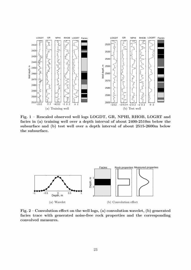
We consider in this case study two wells from the same geological field, a training well and

test well. The facies and well log profiles in the two wells are displayed in Fig.1, and have

been rescaled to 0.1m intervals. In the next section, we estimate all model parameters from

the given facies and well log data in the training well. We then attempt to classify the facies

profile from the well log profiles in the training well, and assess the predictive performance.

Next, we apply the estimated model parameters from the training well when predicting facies

in the test well.

The main interest in this study is on whether the facies predictions improve when we

include in our model convolution effects in the well log profiles and spatial dependency in the

facies profile. Information on the convolution effect introduced by the different logging tools

is typically not given by the logging companies and is challenging to find. Both the vertical

resolution and the expected shape of the convolution effect depend on both the logging speed

4

and the tool specifications. A fictive example displaying the convolution effect is given in

Fig.2. The well log rock properties, in convolution with the given wavelet, constitute the

smoothed measured well log properties which corresponds to the well log data given in Fig.1.

The geological system in this study is a meandering fluvial system, thus the depositional

facies are dominated by processes associated with rivers or streams. These systems are

heterogeneous, i.e. the reservoir properties vary between the facies and also within the

facies. The facies proportions also varies from well to well as can be seen from Fig.1. Facies

is here separated into three possible classes, with properties and description given in Table

1. The facies logs in Fig.1 are interpreted by geologist by use of view cut of the cores and

well logs in cored interval and well logs only in uncored sections. Throughout the depth

interval considered here, the core coverage is high.

The original wireline well logs were logged by the same logging company in the mid 1980’s.

The continuous logs in this study include log-sonic (LOGDT), gamma ray (GR), neutron

porosity (NPHI), bulk density (RHOB) and log-resistivity (LOGRT). The continuous logs

in Fig.1 are centered and normalized, and have also been borehole compensated. Pairwise

scatterplots of the well log observations sorted by facies are displayed in Fig.3, indicating

large overlap between the facies clouds. Some of the tool specifications associated to the

convolution effect are given in Table 2. The approximate vertical resolutions listed are

typical values given from Schlumberger, see Theys (1991) and the references therein, and

represent the minimum thickness of an interval where 90% of the true vertical response occur.

A brief description of each well log according to Theys (1991) follows, with focus on their

respective convolution effects and expected shape as given in Table 2.

The sonic well log, DT, (for which LOGDT is the logarithm of) is a measure of the time

an elastic wave travels through the formation, in particular it is the average delay time for

a received signal emitted from two transmitters. The sonic tool used in this well has two

5

transmitters on either side of four receivers. The vertical resolution of the DT tool is the

spacing between the first and the last receiver. Because only the delay time is measured,

and no signal strength, the expected convolution effect should be uniform.

The gamma ray well log, GR, is a measure of the natural background electromagnetic

radiation from radioactive minerals in the formation with one sensor counting gamma-ray.

Because of natural fluctuations in the background radiation, the vertical resolution of the

GR tool is affected by the logging speed and precision required.

The neutron porosity well log, NPHI, estimates the porosity by measuring the hydrogen

density in the formation by sending fast neutrons (4.5MeV) from a radioactive source. By

elastic collision with nucleus in the formation, the neutrons are gradually slowed down to

thermal neutrons (<0.1eV). Two sensors are counting the thermal neutrons and the difference

between the two sensors are closely related to the density of hydrogen in the formation. The

vertical resolution of the NPHI tool is given by the distance between the sensors.

The bulk density well log, RHOB, estimates the bulk density by measuring the electron

density. The design of the bulk density tool is similar to that of NPHI, but is measuring the

electron density. The radioactive source is emitting high energy gamma-rays which interact

with the electrons in the formation by Compton scattering. The high energy gamma-ray

are gradually transformed into low energy gamma-rays and the electron density is derived

from the difference in low energy signal between two sensors below the source. The vertical

resolution of the RHOB tool is given by the distance between the sensors.

All the nuclear logging tools, GR, NPHI and RHOB, are statistical measurements and

they need to read a signal over time to reach the required precision. We found little infor-

mation for accurate vertical convolution effects, but we expect the convolution shape to be

Gaussian.

The resistivity well log, LOGRT, is a measure of the electrical conductivity of the for-

6

mation. The logging tool in this study has several guard electrodes and one transmitter

electrode which emit a focused electric field into the formation, and a receiver electrode

placed above the guard electrodes. The measurements are most sensitive to the conductivity

of the formation where the electrical field is focused. Because electrical current is conductiv-

ity seeking, the response depends on both the conductivity and geometry of the formation.

The convolution effect is therefor non-linear and thus not trivial. The resistivity log is very

sensitive to the fluid type and often used to estimate the water saturation. If we assume

a simple planar geometry with thick beds, we expect a Gaussian shape of the convolution

effect.

Notation and Model

The well is discretized by a 1D lattice, LT = 1, . . . , T corresponding to the well log

measures with depth intervals of 0.1m. Each depth t is assigned one of the three facies

xt ∈ Ωx : FL,CR,CH. The full facies profile is represented by the full categorical

variable vector x : xt; t = 1, . . . , T which is spatially coupled, see Fig.4(a). Each depth

t is associated with one physical property for each well log, rt = (rt,1, . . . , rt,n), depending

on the facies class at same depth. These physical properties prompts the registrations in

the n well logs. The full response matrix is r : rt; t = 1, . . . , T. The actual well log

observations recorded along the well, as presented in Fig.1, are registered as a convolution

of these responses, see Fig.4(a). The observation matrix is d : dt; t = 1, . . . , T. Each

element in dt is thus a locally weighted average over the true response vector plus an additive

observation noise. A graph for the non-spatial convolution-free NB model is presented in

Fig.4(b) for comparison. Our objective is to predict the facies profile x given the observations

d, making it a convolved inverse problem.

Inference of the categorical facies variables in x is based on a combination of the obser-

7

vations, d, and prior knowledge about x. The solution is represented by the posterior model

which is given by Bayes’ rule:

p(x|d) =1

p(d)× p(d|x)× p(x) . . . . . . . . . . . . . . . . . . . . . . . (1)

Here, p(x) is the prior model, p(d|x) is the likelihood model representing the data col-

lection procedure, and p(d) is a normalizing constant. We choose a prior model for the

facies states according to a Markov chain with a stationary transition matrix, as proposed

in Eidsvik et al. (2004). The full model then becomes a hidden Markov model (HMM)

(MacDonald and Zucchini , 1997). In particular, we denote our model as a convolutional

two-level hidden Markov model according to Rimstad and Omre (2013), as there is an un-

observed continuous level r and convolution in the data collection procedure. Because of the

unobserved level r, the likelihood model is actually an integral of a joint likelihood model in

which r is integrated out. A graphical model of the particular HMM is shown in Fig.4(a).

The major advantage of a Bayesian classification approach is that the posterior model asso-

ciate a probability to every possible solution, enabling us to simulate realizations of the facies

profile and to quantify uncertainties in the classification. The best prediction is defined to

be the maximum aposteriori probability (MAP) prediction.

Prior Model. We assume that the spatial coupling in the facies layers fulfills a first-order

Markov property, p(xt|xt−1, . . . , x1) = p(xt|xt−1), i.e. that the conditional probability of the

facies state xt at step t, given all the previous states, only depends on the single previous

facies state, xt−1. The transition probabilities can be represented by a transition probability

(L×L) matrix P : p(xt|xt−1) : xt, xt−1 ∈ Ωx × Ωx. We assume a stationary Markov model

in which P is depth invariant and that a marginal probability ps(xt) exists. The prior model

for the facies profile is then

p(x) = ps(x1)×T∏

t=2

p(xt|xt−1) . . . . . . . . . . . . . . . . . . . . . . (2)

8

The first-order Markov property is graphically represented by directed arrows between the

xt-variables in Fig.4(a).

We estimate the transition matrix P from the observed well in Fig.1 by counting the

transitions between the classes and then normalize each row. We obtain

P =

FL CR CH

FL 0.9858 0.0047 0.0094

CR 0.0093 0.9813 0.0093

CH 0.0091 0.0023 0.9887

. . . . . . . . . . . . . . . . . . . . (3)

The transition probabilities are given row wise, e.g. the probability of going from CH to FL

upwards is 0.0091. If the sample size of the training set is small, one could assess P by a com-

bination of a data estimate and prior geological knowledge. The sample size for the training

well here is considered sufficiently large, and we estimate P from the data only. We observe

that the diagonal elements are close to unity, indicating that most transitions are into to the

same class as seen in Fig.1. The stationary distribution of P is ps = (0.3920, 0.1544, 0.4536)

which represent the proportion of each facies. The prior model is then fully defined. If the

assumption of a first order Markov chain in the prior is correct, the layer thicknesses should

follow a geometric distribution with parameters on the diagonal of P. The empirical cum-

mulative distribution functions (cdf), compared to geometric cdfs with estimated parameters

for each facies, are displayed in Fig.5. The empirical cdfs have few steps resulting from few

and thick facies layers in the training well, see Fig.1. The fit for class FL is good and a bit

poorer for classes CR and CH. We choose to use a prior Markov chain model regardless of

this slight mismatch.

Likelihood Model. We assume a likelihood model of the form:

p(d|x) =

∫p(d|r)p(r|x)dr . . . . . . . . . . . . . . . . . . . . . . . . . (4)

Here p(d|r) is termed the observation likelihood model and p(r|x) the response likelihood

9

model. In Fig.4(a), the arrows represent dependencies, and we notice that given r, d is

independent of the states x. The response likelihood model, p(r|x), represents physical

response variables related elementwise to the facies states. We assume independent, single-

site Gaussian response likelihood models as indicated in Fig.4(a). The response likelihood

model is

p(r|x) =T∏

t=1

p(rt|xt) ; p(rt|xt) = Nn

(µr|x,Σr|x

), . . . . . . . . . . . . . . (5)

where the mean vector and covariance matrix of p(rt|xt) depend on the class of xt. Elemen-

twise dependencies between the log measures are thus captured by the covariance structure,

Σr|x. The observation likelihood model, p(d|r), is independent for each log and captures the

convolution effect. The observation likelihood model is on the form:

p(d|r) =

n∏

i=1

p(d(i)|r(i)

); p

(d(i)|r(i)

)= NT

(W(i)r(i), σ2

e(i)I), . . . . . . . . (6)

with W(i) being a (T×T )-convolution matrix for well log i and the error term being uncorre-

lated with standard deviation σe(i). Row t in W(i) contain a wavelet, w(i)t , which we assume

to be stationary. The wavelets thus define the weighting of the response variables r(i) giving

observation d(i)t , see Fig.4(a). Because of different logging procedures with corresponding

convolution effects, the well logs are expected to have different convolution wavelets. We

consider convolution wavelets on parametric form, and choose a discretized symmetric beta

model parameterized by (α, β):

Beta(u;α, β) = κ(α, β)[u(1− u)]β−1 , −α ≤ u ≤ α , α ∈ N+ , β ∈ R+ . . . . (7)

Here, α a discrete width parameter, β is a shape parameter and κ(α, β) is a normalizing

constant. Examples of discretized symmetric beta models for equal parameter values of α

and different β are displayed in Fig.6. Observe that the beta model captures both uniform

shapes and hemispherical/bell shapes with finite support on [−α, α].

10

The Gaussian response mean parameter µr|x and the response covariance parameters,

off-diagonal elements of Σr|x, for each facies class x ∈ Ωx are assessed from the training well

by standard maximum likelihood estimation. To avoid convolution effects when performing

this estimation, we have eliminated the ten well log measures on either side of a class transi-

tion, thus assuming that all wavelets are shorter than 2m. The remaining likelihood model

parameters; the response variance parameters, diagonal elements of Σr|x for each facies class

x ∈ Ωx, the wavelets and the noise standard deviation parameters, w(i) and σe(i) for each well

log i = 1, . . . , n, are estimated simultaneously by sample based inference, which can be done

for each well log independently. We use a Markov chain Monte Carlo algorithm, assigning

weak prior distributions to each unknown model parameter and sample values from their

respective posterior distributions. The posterior mean is set as point estimates.

The estimated marginal Gaussian response likelihood models are displayed in Fig.7. We

notice quite large overlap between the classification regions, especially between the classes FL

and CR, while CH tends to be more separable. The wavelet estimates are displayed in Fig.8,

which vertical resolution and shape are summarized in Table 3 along with the noise standard

deviation parameters estimates. Comparing Table 3 to the logging tool specifications in

Table 2, we notice that the estimated LOGDT wavelet is not uniform as expected, and

with a slightly underestimated vertical resolution. The estimated GR, NPHI and RHOB

wavelets slightly overestimate the vertical resolution, while the estimated LOGRT wavelet

has vertical resolution close to the typical numbers. We notice that the estimated wavelets

are quite similar, and with quite short vertical resolution when compared to the dimension of

the well. Also, the estimated white noise variance is quite small, indicating that the model

parameterization emphasizes the response likelihood noise over the observation likelihood

noise.

The likelihood model in Eq.4 must be on a factorisable form to assess the posterior model

11

by the recursive Forward-Backward (FB) algorithm (Baum et al. , 1970; Reeves and Pettitt ,

2004). We approximate the likelihood model according to Rimstad and Omre (2013). A

first order likelihood marginal approximation is of the form:

p (dt|xt) =

∫. . .

∫

n∏

i=1

p∗

(r(i)t

∣∣∣d(i))

p∗

(r(i)t

)

p (rt|xt) dr

(1)t . . . dr

(n)t , . . . . . . . . (8)

where we define the pdfs p∗(r|d) and p∗(r) as Gaussian with analytically tractable parame-

ters. For an expansion to a kth order approximations, which utilize more of the convolution

effect captured in the observation likelihood, we replace the pdfs in Eq.8 with the correspond-

ing kth order marginals of p∗(r|d), p∗(r) and p(r|x) (Rimstad and Omre , 2013). With a

Gaussian response model, this likelihood integral is analytically tractable.

Posterior Model. For the HMM in Fig.4(a) with prior model by Eq.2 and likelihood

model with first order marginal approximations by Eq.8, a first order approximation to the

posterior model in Eq.1 is

p(x|d) = Cd ×

T∏

t=1

p (dt|xt) p(xt|xt−1) . . . . . . . . . . . . . . . . . . . . . (9)

Here Cd is a normalizing constant, and p(x1|x0) = ps(x1) for notational ease. The approx-

imate posterior model is on a factorisable form, and we can thus compute it by the FB

algorithm, see Appendix A. The approximation is expected to perform better for higher

order likelihood approximations, which include more of the spatial well log structure caused

by convolution (Rimstad and Omre , 2013).

Naive Bayesian Model. We will compare our facies classification model to the NB clas-

sifier presented in Li and Anderson-Sprecher (2006) which is found to be superior to many

other statistical approaches. The NB posterior model is still on the form of Eq.1, but with-

out spatial coupling in the prior model and with single-site independent well logs in the

likelihood model:

p(x) =

T∏

t=1

p(xt) , p(d|x) =

T∏

t=1

n∏

i=1

p(d(i)t |xt

). . . . . . . . . . . . . . (10)

12

A graphical model for the NB approach is shown in Fig.4(b), in which we notice that no spa-

tial dependence occur between the facies states and that no convolution is included. For each

state xt, the prior model is the facies proportions in the test well, pprop = (0.3930, 0.1983, 0.4087),

and the likelihood model is the product of the independent univariate well log likelihood

models. Assuming a Gaussian likelihood model, this corresponds to a likelihood model by

Eq.5 with diagonal covariance matrices. The posterior probabilities can thus be computed

independently for each depth t.

Facies Prediction

By solving the inverse problem in a predictive Bayesian framework, we have obtained an ap-

proximate posterior model and in particular elementwise probabilities to each class through-

out the well. A locationwise MAP of the facies profile is computed as

x :

xt = argmax

xt

[p(xt|d)] ; t = 1, . . . , T

. . . . . . . . . . . . . . . . . (11)

As a measure of fit to the true discrete facies profile, we evaluate the locationwise MAP by

the three test statistics mismatch ratio, c1, the difference in facies proportions, c2, and the

difference in transition matrices, c3. These are defined for cv ∈ [0, 1]; v = 1, 2, 3 as

c1 =1

T

T∑

t=1

I(xt = xt) . . . . . . . . . . . . . . . . . . . . . . . . . (12)

c2 = 1−1

M

M∑

m=1

|pMAPprop,m − pprop,m| . . . . . . . . . . . . . . . . . . . . (13)

c3 = 1−1

M

M∑

m=1

|PMAPm,m − Pm,m| , . . . . . . . . . . . . . . . . . . . . (14)

where pMAPprop and PMAP are the proportions and transition matrix estimated from the MAP

and pprop and P the true proportions and transition matrix in Eq.3 estimated from the true

facies profile. Observe that c3 is defined from the estimated transition matrices diagonal

elements only, and can hence be regarded as a measure of how well we predict the thickness

13

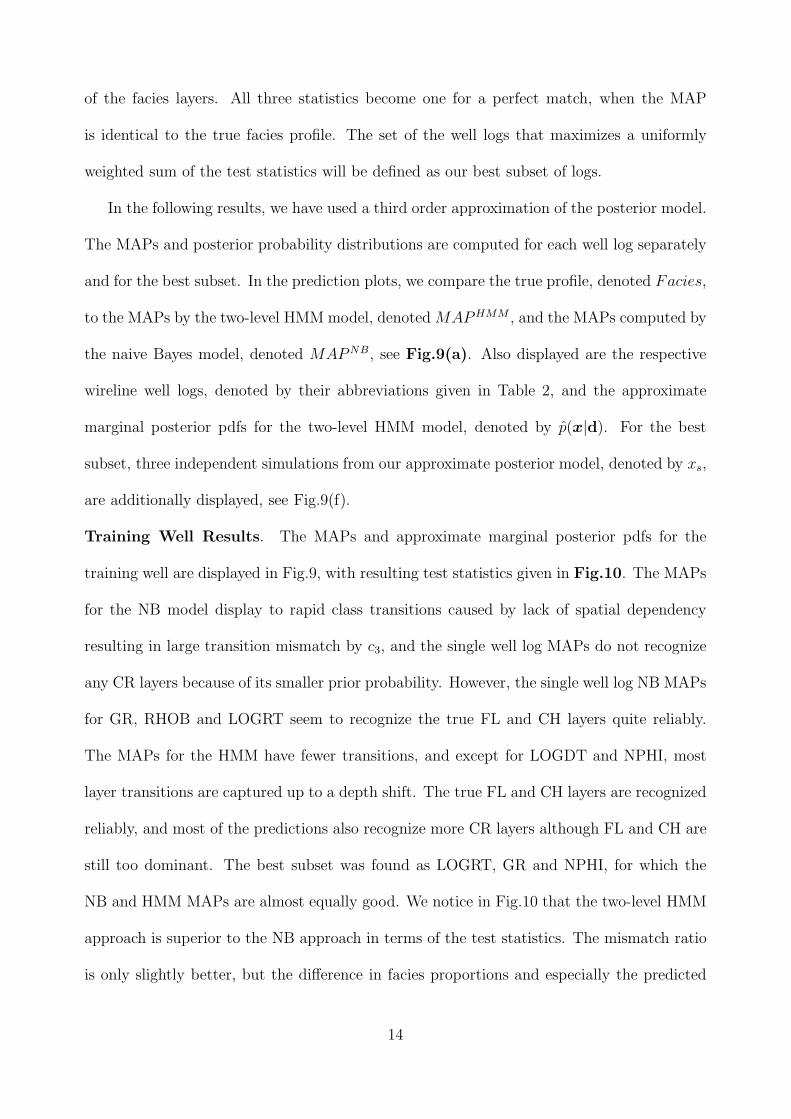
of the facies layers. All three statistics become one for a perfect match, when the MAP

is identical to the true facies profile. The set of the well logs that maximizes a uniformly

weighted sum of the test statistics will be defined as our best subset of logs.

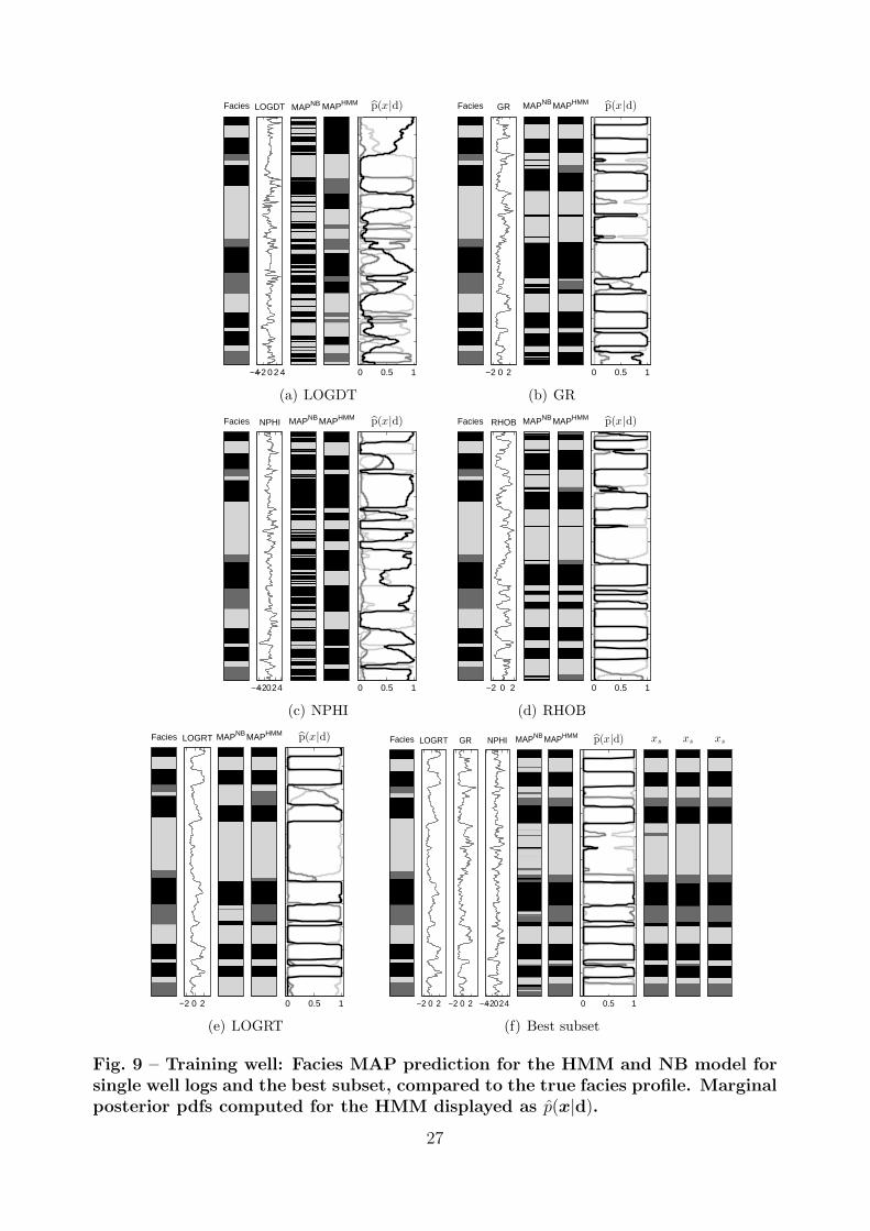
In the following results, we have used a third order approximation of the posterior model.

The MAPs and posterior probability distributions are computed for each well log separately

and for the best subset. In the prediction plots, we compare the true profile, denoted Facies,

to the MAPs by the two-level HMM model, denoted MAPHMM , and the MAPs computed by

the naive Bayes model, denoted MAPNB, see Fig.9(a). Also displayed are the respective

wireline well logs, denoted by their abbreviations given in Table 2, and the approximate

marginal posterior pdfs for the two-level HMM model, denoted by p(x|d). For the best

subset, three independent simulations from our approximate posterior model, denoted by xs,

are additionally displayed, see Fig.9(f).

Training Well Results. The MAPs and approximate marginal posterior pdfs for the

training well are displayed in Fig.9, with resulting test statistics given in Fig.10. The MAPs

for the NB model display to rapid class transitions caused by lack of spatial dependency

resulting in large transition mismatch by c3, and the single well log MAPs do not recognize

any CR layers because of its smaller prior probability. However, the single well log NB MAPs

for GR, RHOB and LOGRT seem to recognize the true FL and CH layers quite reliably.

The MAPs for the HMM have fewer transitions, and except for LOGDT and NPHI, most

layer transitions are captured up to a depth shift. The true FL and CH layers are recognized

reliably, and most of the predictions also recognize more CR layers although FL and CH are

still too dominant. The best subset was found as LOGRT, GR and NPHI, for which the

NB and HMM MAPs are almost equally good. We notice in Fig.10 that the two-level HMM

approach is superior to the NB approach in terms of the test statistics. The mismatch ratio

is only slightly better, but the difference in facies proportions and especially the predicted

14

layer thickness are much better because of the NB predictions lack of CR layers and too

rapid transitions. The predictions for the best subset are however almost as good.

The approximate posterior pdfs are dominated by probabilities close to one or zero,

which occurs because the unknown model parameters are set to the best point-estimates,

hence omitting model parameter uncertainty. By approaching the problem in a hierarchical

Bayesian inversion setting we can assess these uncertainties more reliably (Rimstad et al. ,

2012), but this is not considered in this study.

The NB approach has significantly less computational demands than the HMM approach,

as it ignores the spatial coupling. All computations in this study are however run within

minutes on a standard work station for both approaches. In practice, the computational de-

mands are therefor small also for the HMM approach even for the third order approximation

considered throughout this study.

Test Well Results. We now consider facies prediction from the wireline well logs in the

test well displayed in Fig.1(b), utilizing the model parameters estimated in the training well.

The MAP predictions and approximate marginal posteriors pdfs for the best subset in the

test well are displayed in Fig.11, with resulting test statistics given in Fig.12 in which the

test statistic results for single well logs is also displayed. We observe the same trends as

for the predictions in the training well, with the HMM being superior to the NB model in

terms of the test statistics. Neither model identifies the CR layers particularly reliable, as

the true facies profile in the test well has significantly different class proportions than the

training well. The CH layers are reliably identified which is important because it is the most

interesting geological class in terms of possible occurrence of hydrocarbons.

15

Conclusion

We have predicted facies from multiple wireline well logs for real well data from a geological

field offshore Norway. The inversion, and the associated parameter estimation, is solved by

discretizing the well in a Bayesian predictive framework. By choosing a prior Markov model,

we are able to incorporate stationary vertical facies dependencies throughout the well. We

next introduce a continuous hidden level in the likelihood model representing correlated

physical properties for each discrete facies element in the well. Assuming that the actual

wireline well log observations are captured as a weighted sum of this hidden level, we are

able to incorporate the convolution effect originating from the different logging tools.

Predictions from our model are compared to predictions from a naive Bayesian classifier.

The naive model neglects both spatial dependency, possible correlated wireline well logs and

convolution effect. Results from the blind test well indicate that our model outperforms the

naive model slightly in terms of correct facies identification. However, the major improvement

comes in terms of predicting correct facies proportions and layer thickness, hence providing

predictions with more realistic geological properties. These results seem to origin from

the Markov chain assumption, while inclusion of convolution effect tend to be less influent

in the field case considered, as the estimated convolution width is small compared to the

well scale. We therefor believe the proposed model should work reliably also on well pairs

logged by different logging companies, i.e. with different vertical resolutions, which should

be studied further. In such studies, a parameter prior model should be set on the convolution

parameters, taking into account parameter uncertainty and differences between the logging

tools. Of the five well log measures considered, the combination of the log-resistivity, gamma

ray and neutron porosity logs were is identified as the best subset for facies prediction in the

geological field of this study.

16

Nomenclature

cv = facies prediction test statistics, v = 1, 2, 3Cd = normalizing constantd = matrix with observed convolved well log profilesdt = vector with observed well log values at depth t

d(i) = observed well log profile i

i = well log index, i = 1, . . . , nLT = 1D latticeL = number of facies classesn = number of well log profiles

p(•) = probability density function for variable •ps(xt) = marginal probability for facies at depth t

pprop = proportions of facies in wellp∗(•) = Gaussian approximate distribution for variable •

P = facies transition matrixr = matrix with physical property profilesrt = physical property vector at depth t

r(i) = physical property profile for well log i

t = depth, L, mT = length of LT

w = convolution waveletw(i) = convolution wavelet for well log i

W = wavelet matrixW(i) = wavelet matrix for well log i

x = facies profile vectorxt = facies class at depth t

α = Beta wavelet length parameterβ = Beta wavelet shape parameter

κ(α, β) = Beta wavelet normalizing constantµr|x = physical property mean vector for facies xσe = noise standard deviation

σe(i) = noise standard deviation for well log i

Σr|x = physical property covariance matrix for facies xΩx = set of facies classes

Acknowledgments

The work is part of the Uncertainty in reservoir Evaluation (URE) activity - consortium at

Department of Mathematical Sciences, NTNU, Trondheim, Norway. We would like to thank

Statoil for providing us with well log data and also specially to Alf Birger Ruestad for helpful

discussions and comments.

17

References

1. Baum, L.E., Petrie, T., Soules, G., and Weiss, N. (1970). ”A Maximization Technique

Occurring in the Statistical Analysis of Probabilistic Functions of Markov Chains.”

The Annals of Mathematical Statistics, 41, No.1.

2. Chang, H., Chen, H., and Fang, J, (1997). ”Lithology Determination From Well Logs

With Fuzzy Associative Memory Neural Network.” IEEE Transactions on Geoscience

and Remote Sensing, 35, No.3.

3. Coudert, L., Frappa, M., and Arias, R. (1994). ”A Statistical Method for Litho-Facies

Identification.” J. of Applied Geophysics, 32, p.257-267.

4. Cuddy, S.J., (2000). ”Litho-Facies and Permeability Prediction From Electrical Logs

Using Fuzzy Logic.” SPE Res Eval & Eng, 3, No.4.

5. Eidsvik, J., Mukerji, T., and Switzer, P., (2004). ”Estimation of Geological Attributes

From a Well Log: An Application of Hidden Markov Chains.”Mathematical Geology,

36, No.3.

6. Guo, G., Diaz, M.A., Paz, F., Smalley, J., and Waninger, E.A., (2007). ”Rock Typing

as an Effective Tool for Permeability and Water-Saturation Modeling: A Case Study

in a Clastic Reservoir in the Oriente Basin.” SPE Res Eval & Eng, 10, No.6.

7. Kaaresen, K.F., and Taxt, T., (1998). ”Multichannel Blind Deconvolution of Seismic

Signals.”Geophysics, 63, No.6.

8. Larsen, A.L., Ulvmoen, M., Omre, H., and Buland, A., (2006). ”Bayesian Litholo-

gy/Fluid Prediction and Simulation on the Basis of a Markov-Chain Prior Model.”

Geophysics, 71, No.5.

18

9. Li, Y., and Anderson-Sprecher, R., (2006). ”Facies Identification From Well Logs: A

Comparison of Discriminant Analysis and Naive Bayes Classifier.” J. of Petroleum

Science and Eng., 53, p.149-157.

10. Loures, L.G.L., and Moraes, F.S., (2006). ”Porosity Inference and Classification of

Siliciclastic Rocks From Multiple Data Sets.”Geophysics, 71, No.5.

11. MacDonald, I. and Zucchini, W., (1997). Hidden Markov and Other Models for

Discrete- valued Time Series, London, New York: Chapman & Hall.

12. Perez, H.H., Datta-Gupta, A., and Mishra, S., (2005). ”The Role of Electrofacies,

Lithofacies and Hydraulic Flow Units in Permeability Predictions From Well Logs: A

Comparative Analysis Using Classification Trees.” SPE Res Eval & Eng, 8, No.3.

13. Qi, L., and Carr, T.R., (2006). ”Neural Network Prediction of Carbonate Lithofacies

From Well Logs, Big Bow and Sand Arroyo Creek Fields, Southwest Kansas.” Com-

puters & Geosciences, 32, p.947-964.

14. Reeves, R., and Pettitt, A.N., (2004). ”Efficient Recursions for General Factorisable

Models.” Biometrika, 91, p.751-757.

15. Rimstad, K., Avseth, P., and Omre, H., (2012). ”Hierarchical Bayesian Lithology/Fluid

Prediction: A North Sea Case Study.”Geophysics, 77, No.2.

16. Rimstad, K., and Omre, H., (2013). ”Approximate Posterior Distributions for Convolu-

tional Two-Level Hidden Markov Models.”Computational Statistics & Data Analysis,

58, p.187-200.

17. Tang, H., and Ji, H., (2006). ”Incorporation of Spatial Characters Into Volcanic Facies

and Favorable Reservoir Prediction.” SPE Res Eval & Eng, 9, No.4.

19

18. Tang, H., Toomey, N., and Meddaugh, W.S., (2011). ”Using an Artificial-Neural-

Network Method to Predict Carbonate Well Log Facies Successfully.” SPE Res Eval &

Eng, 14, No.1.

19. Tang, H., and White, C.D., (2008). ”Multivariate Statistical Log Log-Facies Classifica-

tion on a Shallow Marine Reservoir.” J. of Petroleum Science and Eng., 61, p.88-93.

20. Theys, P.P., (1991). Log Data Acquisition and Quality Control, Editions TECHNIP.

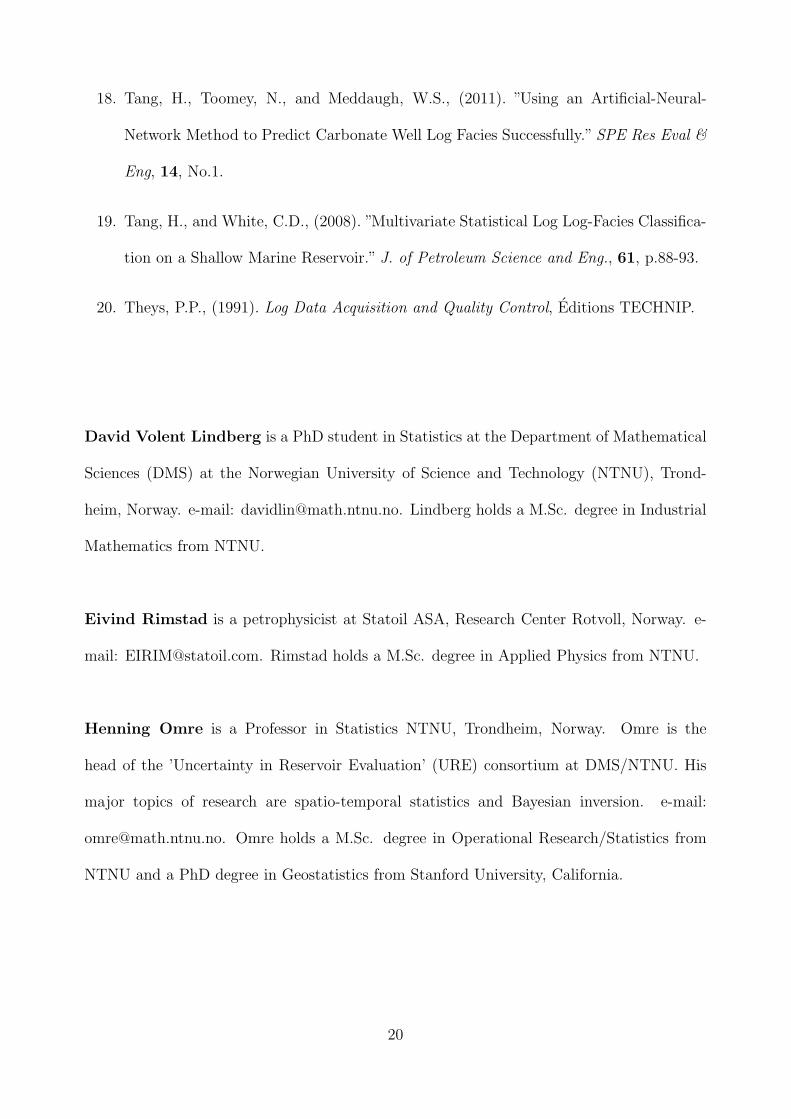
David Volent Lindberg is a PhD student in Statistics at the Department of Mathematical

Sciences (DMS) at the Norwegian University of Science and Technology (NTNU), Trond-

heim, Norway. e-mail: davidlin@math.ntnu.no. Lindberg holds a M.Sc. degree in Industrial

Mathematics from NTNU.

Eivind Rimstad is a petrophysicist at Statoil ASA, Research Center Rotvoll, Norway. e-

mail: EIRIM@statoil.com. Rimstad holds a M.Sc. degree in Applied Physics from NTNU.

Henning Omre is a Professor in Statistics NTNU, Trondheim, Norway. Omre is the

head of the ’Uncertainty in Reservoir Evaluation’ (URE) consortium at DMS/NTNU. His

major topics of research are spatio-temporal statistics and Bayesian inversion. e-mail:

omre@math.ntnu.no. Omre holds a M.Sc. degree in Operational Research/Statistics from

NTNU and a PhD degree in Geostatistics from Stanford University, California.

20

Appendix A: Forward-backward algorithm

A first order forward-backward algorithm is presented, for a higher order generalization see

Reeves and Pettitt (2004).

Algorithm: Forward-Backward algorithm

Forward:

• Initiate:

pf (x1) = Cx1 · p(dt|x1)p(x1)

Cx1 =1∑

x1p(dt|x1)p(x1)

• Iterate for t = 2, . . . , T :

pf (xt−1, xt) = Cxt−1,t · p(dt|xt)p(xt|xt−1)pf(xt−1)

Cxt−1,t =1∑

xt−1

∑xt

p(dt|xt)p(xt|xt−1)pf (xt−1)

pf (xt) =∑

xt−1Cxt−1,t · p(dt|xt)p(xt|xt−1)pf(xt−1)

Backward:

• Initiate:

pb(xT ) = pf (xT )

• Iterate for t = T, . . . , 2:

pb(xt−1|xt) =pf (xt−1,xt)

pf (xt)

pb(xt−1) =∑

xtpb(xt−1|xt)pb(xt)

pb(xt|xt−1) =pb(xt−1|xt)pb(xt)

pb(xt−1)

The full posteriori distribution is computed by

p(x|d) =

T∏

t=1

p(xt|xt−1,d) = pb(x1)

T∏

t=2

pb(xt|xt−1) .

For simulation from the posterior distribution, sample xs1 ∼ pb(x1) and then sample xs

t ∼

pb(xt|xst−1) for t = 2, . . . , T . Then x

s = (xs1, . . . , x

sT ) is a realization simulated from the

posterior model p(x|d).

21

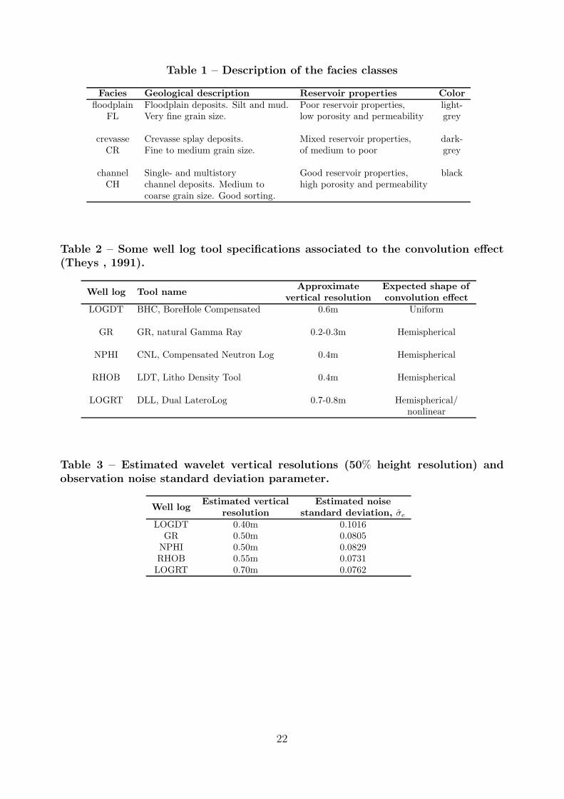
Table 1 – Description of the facies classes

Facies Geological description Reservoir properties Color

floodplain Floodplain deposits. Silt and mud. Poor reservoir properties, light-FL Very fine grain size. low porosity and permeability grey

crevasse Crevasse splay deposits. Mixed reservoir properties, dark-CR Fine to medium grain size. of medium to poor grey

channel Single- and multistory Good reservoir properties, blackCH channel deposits. Medium to high porosity and permeability

coarse grain size. Good sorting.

Table 2 – Some well log tool specifications associated to the convolution effect(Theys , 1991).

Well log Tool nameApproximate Expected shape of

vertical resolution convolution effect

LOGDT BHC, BoreHole Compensated 0.6m Uniform

GR GR, natural Gamma Ray 0.2-0.3m Hemispherical

NPHI CNL, Compensated Neutron Log 0.4m Hemispherical

RHOB LDT, Litho Density Tool 0.4m Hemispherical

LOGRT DLL, Dual LateroLog 0.7-0.8m Hemispherical/nonlinear

Table 3 – Estimated wavelet vertical resolutions (50% height resolution) andobservation noise standard deviation parameter.

Well logEstimated vertical Estimated noise

resolution standard deviation, σe

LOGDT 0.40m 0.1016GR 0.50m 0.0805

NPHI 0.50m 0.0829RHOB 0.55m 0.0731LOGRT 0.70m 0.0762

22

−2 0 2

2410

2420

2430

2440

2450

2460

2470

2480

2490

2500

2510

LOGDT

Wel

l dep

th, m

0 2

GR

−4−202

NPHI

−2 0 2

RHOB

0 2

LOGRT Facies

(a) Training well−2 0 2

2520

2530

2540

2550

2560

2570

2580

2590

2600

LOGDT

Wel

l dep

th, m

−2 0 2 4

GR

−2 0 2

NPHI

−2 0 2

RHOB

0 2

LOGRT Facies

(b) Test well

Fig. 1 – Rescaled observed well logs LOGDT, GR, NPHI, RHOB, LOGRT andfacies in (a) training well over a depth interval of about 2400-2510m below thesubsurface and (b) test well over a depth interval of about 2515-2600m belowthe subsurface.

−1 −0.5 0 0.5 1Depth, m

(a) Wavelet

Facies

Dep

th, m

1

2

3

Rock properties Measured properties

(b) Convolution effect

Fig. 2 – Convolution effect on the well logs, (a) convolution wavelet, (b) generatedfacies trace with generated noise-free rock properties and the correspondingconvolved measures.

23

−2 0 2 4

LOG

DT

−2 0 2 4

−1

0

1

2

3

GR

−1 0 1 2 3

−2 0 2 4

−4

−2

0

2

NP

HI

−1 0 1 2 3

−4

−2

0

2

−4 −2 0 2

−2 0 2 4

−2

−1

0

1

2

RH

OB

−1 0 1 2 3

−2

−1

0

1

2

−4 −2 0 2

−2

−1

0

1

2

−2 0 2

−2 0 2 4

−1

0

1

2

LOG

RT

LOGDT−1 0 1 2 3

−1

0

1

2

GR−4 −2 0 2

−1

0

1

2

NPHI−2 0 2

−1

0

1

2

RHOB−1 0 1 2

LOGRT

Fig. 3 – Pairwise scatterplots and histograms of the training well log data sortedby facies class.

24

d1

d2

...

dT−1

dT

r1

r2

...

rT−1

rT

x1

x2

...

xT−1

xT

(a) Two-level HMM

d1

d2

...

dT−1

dT

x1

x2

...

xT−1

xT

(b) NB model

Fig. 4 – Directed acyclic graph of (a) the convolutional two-level HMM and (b)the NB model for observed data d = (d1, . . . , dT ) with latent fields r = (r1, . . . , rT )and x = (x1, . . . , xT ). The directed arrows represent dependencies between thevariables.

0 100 2000

0.2

0.4

0.6

0.8

1FL

0 100 2000

0.2

0.4

0.6

0.8

1CR

0 100 2000

0.2

0.4

0.6

0.8

1CH

Fig. 5 – Empirical cdf (dashed) vs geometric cdf (solid) for class layers.

25

β=1

−α α

β=20

β=5β=2

Fig. 6 – Discretized symmetric beta model, Beta(u;α, β), for equal width param-eter α = 7 and different shape parameters β.

−4 −2 0 2 4

(a) LOGDT

−4 −2 0 2 4

(b) GR

−4 −2 0 2 4

(c) NPHI

−4 −2 0 2 4

(d) RHOB

−4 −2 0 2 4

(e) LOGRT

Fig. 7 – Marginal Gaussian response likelihood models for FL in solid light-gray,CR in dashed dark-gray and CH in solid black.

−0.6 −0.4 −0.2 0 0.2 0.4 0.60

0.1

0.2

0.3

(a) LOGDT

−0.6 −0.4 −0.2 0 0.2 0.4 0.60

0.1

0.2

0.3

(b) GR

−0.6 −0.4 −0.2 0 0.2 0.4 0.60

0.1

0.2

0.3

(c) NPHI

−0.6 −0.4 −0.2 0 0.2 0.4 0.60

0.1

0.2

0.3

(d) RHOB

−0.6 −0.4 −0.2 0 0.2 0.4 0.60

0.1

0.2

0.3

(e) LOGRT

Fig. 8 – Estimated Beta parameterized wavelets plotted against length in m.

26

Facies

−4−2 0 2 4

LOGDT MAPNB MAPHMM

0 0.5 1

p(x|d)

(a) LOGDT

Facies

−2 0 2

GR MAPNB MAPHMM

0 0.5 1

p(x|d)

(b) GR

Facies

−4−20 2 4

NPHI MAPNB MAPHMM

0 0.5 1

p(x|d)

(c) NPHI

Facies

−2 0 2

RHOB MAPNB MAPHMM

0 0.5 1

p(x|d)

(d) RHOB

Facies

−2 0 2

LOGRT MAPNB MAPHMM

0 0.5 1

p(x|d)

(e) LOGRT

Facies

−2 0 2

LOGRT

−2 0 2

GR

−4−20 2 4

NPHI MAPNB MAPHMM

0 0.5 1

p(x|d) xs xs xs

(f) Best subset

Fig. 9 – Training well: Facies MAP prediction for the HMM and NB model forsingle well logs and the best subset, compared to the true facies profile. Marginalposterior pdfs computed for the HMM displayed as p(x|d).

27

LOGDT GR NPHI RHOB LOGRT Subset0.5

0.6

0.7

0.8

0.9

1

c1

LOGDT GR NPHI RHOB LOGRT Subset

0.8

0.9

1

c2

LOGDT GR NPHI RHOB LOGRT Subset

0.7

0.8

0.9

1

c3

Fig. 10 – Test statistics for the MAPs in the training well, NB in gray and HMMin black.

Facies

−2 0 2

LOGRT

−20 2 4

GR

−20 2

NPHI MAPNB MAPHMM

0 0.5 1

p(x|d) xs xs xs

Fig. 11 – Test well: Facies MAP prediction for the HMM and NB model for thebest well log subset, compared to the true facies profile.

LOGDT GR NPHI RHOB LOGRT Subset

0.3

0.4

0.5

0.6

0.7

0.8

0.9

1

c1

LOGDT GR NPHI RHOB LOGRT Subset

0.8

0.9

1

c2

LOGDT GR NPHI RHOB LOGRT Subset

0.7

0.8

0.9

1

c3

Fig. 12 – Test statistics for the MAPs in the test well, NB in gray and HMM inblack.

28