Embed Size (px)
Citation preview

NASA Contractor Report 187126
Investigation of Advanced Counterrotation
Blade Configuration Concepts for High Speed
Turboprop Systems
Task 5
Final Report
- Unsteady Counterrotation Ducted Propfan Analysis
¢¢t
I ,-- 0
0 _ CZ D 0
Edward J. Hall and Robert A. Delaney
Allison Gas Turbine Division of General Motors
Indianapolis, Indiana
January 1993
Prepared for
Lewis Research Center
Under Contract NAS3-25270
O
it
oo
Z I_o
Owed
_..._ < D O rn
_- Z t.L o Z __
_-_ ;'--l_J cn _-- .-- L
¢,,11...- U3_.-t/_ _..
I _ r_ ,_
I _.9 _D _ _ k.


Preface
This report was prepared by Edward J. Hall and Robert A. Delaney of the Allison
Gas Turbine Division, General Motors Corporation, Indianapolis, IN. The work was
performed under NASA Contract NAS3-25270 from April, 1991 to September, 1992.
The flow code theory, and programming modifications necessary for the aerodynamic
analysis were performed by Edward J. Hall. The Allison program manager for this
contract was Robert A. Delaney. The NASA project manager for this contract was
Christopher J. Miller.
Acknowledgements
The authors would like to express their appreciation to the following NASA
personnel who contributed to this program:
Dr. John. J. Adamczyk for the many helpful technical discussions concerning
the development of the computer codes,
Dr. Christopher J. Miller for his suggestions and critical review of the program,
Dr. Andrea Arnone and Dr. Charles Swanson for their assistance during the
development of the multigrid algorithm.
The services of the NASA Numerical Aerodynamic Simulation (NAS) facilities
and personnel are gratefully acknowledged.
UNIX is a trademark of AT&T
IRIS is a trademark of Silicon Graphics, Inc.
AIX is a trademark of IBM
UNICOS is a trademark of Cray Computers
PostScript is a trademark of Adobe Systems, Inc.
°..
111
PRONG P/_IGE BLANK NOT FILMED

TABLE OF CONTENTS
NOTATION .................................... xi
ABBREVIATIONS ............................... xv
1. SUMMARY ................................. 1
2. INTRODUCTION ............................. 3
3. 3D EULER/NAVIER-STOKES NUMERICAL ALGORITHM . 11
3.1 Nondimensionalization .......................... 11
3.2 3-D Navier-Stokes Equations ....................... 12
3.3 2-D Navier-Stokes Equations with Embedded Blade Row Body Forces 16
3.4 Numerical Formulation .......................... 18
3.5 Runge-Kutta Time Integration ...................... 25
3.6 Fluid Properties .............................. 27
3.7 Dissipation Function ........................... 27
3.8 Implicit Residual Smoothing ....................... 29
3.9 Turbulence Model ............................. 32
3.10 Multigrid Convergence Acceleration ................... 34
3.11 Single Block Boundary Conditions .................... 38
3.12 Multiple-Block Coupling Boundary Conditions ............. 41
3.13 Solution Procedure ............................ 49
4. RESULTS .................................. 51
4.1 2-D Compressor Cavity Flow (Steady Flow) .............. 51
4.2 Model Counterrotating Propfan (Steady Flow) ............. 54
4.3 NASA 1.15 Pressure Ratio Fan (Steady Flow) ............. 60
4.4 GMA3007 Fan Section (Steady Flow) .................. 71
4.5 Oscillating Flat Plate Cascade (Unsteady Flow) ............ 79
iv

4.6 SR7 Unducted Propfan -CylindricalPost InteractionStudy (Unsteady86
Flow) ...................................
4.7 Model Counterrotating Propfan (Unsteady Flow) ........... 92
4.8 GMA3007 Fan Section Distortion Study (Unsteady Flow) ....... 100
1095. CONCLUSIONS ..............................
111REFERENCES ..................................
APPENDIX A. ADPAC DISTRIBUTION LIST ............. 117

LIST OF FIGURES
Figure 2.1:
Figure 2.2:
Figure 3.1:
Figure 3.2:
Figure 3.3:
Figure 3.4:
Figure 3.5:
Figure 3.6:
Figure 3.7:
Figure 3.8:
Figure 3.9:
Figure 3.10:
Figure 3.11:
Figure 3.12:
Figure 4.1:
Figure 4.2:
Ultra High Bypass Propulsor aerodynamic characteristics . . 4
Computational Schemes for Multiple Blade Row Turboma-
chinery .............................. 6
ADPAC-AOACR Cylindrical Coordinate System Reference 14
ADPAC-AOACR 2-D Single Block Mesh Structure Illustration 19
ADPAC-AOACR 2-D Two Block Mesh Structure Illustration 20
ADPA C-A OA CR 2-D Multiple Block Mesh Structure Illustra-
tion ................................ 21
Three-dimensional finite volume cell .............. 23
Multigrid Mesh Coarsening Strategy and Mesh Index Relation 36
Multigrid V Cycle Strategy ................... 37
2-D Mesh Block Phantom Cell Representation ........ 39
ADPAC-AOACR Contiguous Mesh Block Coupling Scheme 42
ADPAC-AOACR Non-Contiguous Mesh Block Coupling Scheme 44
ADPAC-AOACR Circumferential Averaging (Mixing Plane)
Mesh Block Coupling Scheme for Multiple Blade Row Calcu-
lations .............................. 46
ADPAC-AOACR Time/Space Resolved Mesh Block Coupling
Scheme for Multiple Blade Row Calculations ......... 48
Inner Banded Stator Cavity Geometry and ADPAC-AOACR
2-D Mesh System ........................ 52
ADPAC-AOACR Full Multigrid Convergence History for 2-D
Inner Banded Stator Cavity Flow Calculation ......... 53
vi
Figure 4.3:
Figure 4.4:
Figure 4.5:
Figure 4.6:
Figure 4.7:
Figure 4.8:
Figure 4.9:
Figure 4.10:
Figure 4.11:
Figure 4.12:
Figure 4.13:
Figure 4.14:
Figure 4.15:
ADPA C-A OA CR Predicted Velocity Vectors for 2-D Inner Banded
Stator Cavity Flow Analysis .................. 54
Model Counterrotating Propfan Model Geometric and Aero-
dynamic Design Parameters .................. 56
ADPAC-AOACR Two-Block Mesh System for Steady Flow
Analysis of Model Counterrotating Propfan .......... 57
ADPAC-AOACR Multigrid Convergence History for Model
Counterrotating Propfan Steady Flow Analysis Based on Mix-
ing Plane Concept ........................ 58
ADPA C-A OA CR Predicted Steady Surface Static Pressure Coun-
tours and Post Rotor Static Pressure Contours for Model Coun-
terrotating Propfan ....................... 59
ADPAC-AOACR Predicted Steady Axisymmetric Averaged
Mach Number Contours for Model Counterrotating Propfan . 61
ADPAC-AOACR Predicted Steady Axisymmetric Averaged
Static Pressure Contours for Model Counterrotating Propfan 62
ADPA C-A OA CR Predicted Steady Circumferential Blade-to-
Blade Static Pressure Contours for Model Counterrotating
Propfan .............................. 63
NASA 1.15 Pressure Ratio Fan Geometry and Design Param-
eters ............................... 64
ADPAC-AOACR Four Block Mesh System for NASA 1.15
Pressure Ratio Fan ....................... 65
A DPA C-A OA CR Predicted Axisymmetric Averaged Flow Ab-
solute Mach Number Contours for NASA 1.15 Presure Ratio
Fan ................................ 67
ADPA C-A OA CR Predicted Axisymmetric Averaged Flow Static
Pressure Contours for NASA 1.15 Presure Ratio Fan ..... 68
Comparison of Predicted and Experimental Stator Exit Radial
Total Pressure Ratio Distribution for NASA 1.15 Pressure Ra-
tio Fan (M=0.75) ........................ 69
vii

Figure 4.16:
Figure 4.17:
Figure 4.18:
Figure 4.19:
Figure 4.20:
Figure 4.21:
Figure 4.22:
Figure 4.23:
Figure 4.24:
Figure 4.25:
Figure 4.26:
Figure 4.27:
Figure 4.28:
Figure 4.29:
Figure 4.30:
ADPAC-AOACR Predicted 3-D Surface Static Pressure Con-
tours for NASA 1.15 Pressure Ratio Fan (M=0.75) ...... 70
Allison GMA3007 Fan Section Geometry ........... 72
Axisymmetric Detail of ADPA C-A OA CR Three-Block Mesh
System for Allison GMA3007 Fan Section ........... 73
Circumferential Detail of ADPA C-A OA CR Three-Block Mesh
System for Allison GMA3007 Fan Section ........... 74
Comparison of Predicted and Experimental Radial Total Pres-
sure Ratio Distributions Downstream of Fan Rotor for Allison
GMA3007 Fan Section ..................... 75
Comparison of Predicted and Experimental Radial Total Pres-
sure and Total Temperature Ratio Distributions at Bypass
Vane Leading Edge for Allison GMA3007 Fan Section .... 76
Predicted Axisymmetric-Averaged Static Pressure Contours
for Allison GMA3007 Fan Section ............... 77
Predicted Surface Static Pressure Contours for Allison GMA3007
Fan Section ........................... 78
Oscillating Flat Plate Cascade Geometry ........... 81
Oscillating Flat Plate Cascade Blade to Blade Mesh Systems 82
Comparison of ADPA C-A OA CR Prediction and Smith Linear
Theory for Real Component of Airfoil Surface Pressure Re-
sponse for the Oscillating Flat Plate Cascade Test Case . . 84
Comparison of ADPA C-A OA CR Prediction and Smith Linear
Theory for Imaginary Component of Airfoil Surface Pressure
Response for the Oscillating Flat Plate Cascade Test Case . . 85
SR7 Propfan - Cylindrical Post Interaction Study Experimen-
tal Configuration ........................ 87
Geometric and Aerodynamic Design Parameters for the Orig-
inal SR7 Propfan ........................ 88
SR7 Propfan - Cylindrical Post Aerodynamic Interaction Ex-
perimental Airfoil Surface Data Locations ........... 90
viii

Figure 4.31:
Figure 4.32:
Figure 4.33:
Figure 4.34:
Figure 4.35:
Figure 4.36:
Figure 4.37:
Figure 4.38:
Figure 4.39:
Figure 4.40:
Figure 4.41:
ADPAC-AOACR Two-Block Mesh System for SR7 Propfan
Cylindrical Post Time-Dependent Aerodynamic Interaction
Analysis ............................. 91
Comparison of Time-Resolved Predicted and Experimental
Propfan Surface Static Pressure Histories for SR7 Propfan -
Cylindrical Post Aerodynamic Interaction Study (10.0% Axial
Chord, 64.1% Radial Span,Suction Side) ........... 93
Comparison of Time-Resolved Predicted and Experimental
Propfan Surface Static Pressure Histories for SR7 Propfan -
Cylindrical Post Aerodynamic Interaction Study (36.7% Axial
Chord, 64.1% Radial Span, Suction Side) ........... 94
Comparison of Time-Resolved Predicted and Experimental
Propfan Surface Static Pressure Histories for SR7 Propfan -
Cylindrical Post Aerodynamic Interaction Study (10.0% Axial
Chord, 64.1% Radial Span, Pressure Side) ........... 95
Comparison of Time-Resolved Predicted and Experimental
Propfan Surface Static Pressure Histories for SR7 Propfan -
Cylindrical Post Aerodynamic Interaction Study (36.7% Axial
Chord, 64.1% Radial Span, Pressure Side) ........... 96
Predicted Instantaneous Propfan Airfoil Midspan Total Pres-
sure Contours for Cylinder/Propfan Interaction Study .... 97
ADPAC-AOACR Time-Accurate Residual History for Model
Counter-Rotating Propfan Aerodynamic Interaction Analysis 99
ADPA C-A OA CR Predicted Instantaneous Static Pressure Con-
tours at Midspan (1 cycle of time-periodic solution) ..... 101
Total Pressure Deficit Pattern for Allison GMA3007 Engine
Fan Section Distortion Study .................. 102
ADPA C-A OA CR 10-Block Mesh System for Allison GMA3007
Engine Fan Section Inlet Distortion Study .......... 104
ADPA C-A OA CR Instantaneous Predicted Rotor Surface Static
Pressure Contours for GMA3007 Fan Operating Under Inlet
Distortion ............................ 106
ix

Figure 4.42: A DPA C-A OA CR Predicted Instantaneous Total Pressure Con-
tours at 30% Axial Chord for the GMA3007 Fan Operating
Under Inlet Distortion ...................... 107
X

NOTATION
A listof the symbols used throughout this document and their definitionsis
provided below for convenience. Parameter values are shown in parentheses.
Roman Symbols
ao J
c,•
e.
j.k.
kr
_7.
p.
r
V
Z.
• speed of sound
• airfoil chord
.. specific heat at constant pressure
.. specific heat at constant volume
• internal energy
first grid index of numerical solution
• second grid index of numerical solution
• third grid index of numerical solution or thermal conductivity
.. reduced frequency kr = ¢ac/(2V)
turbulence model damping function
• time step index of numerical solution or rotational speed (revolutions/sec)
• outward unit normal vector
pressure
radius or cylindrical radial coordinate
time
• velocity
• first Cartesian coordinate
• second Cartesian coordinate
• cylindrical axial coordinate or third Cartesian coordinate
A... surface area
A + ... turbulence model parameter
xi

B... number of propeller blades
Cp... power coefficient (Cp = V/pn 3 D 5)
Ct . . . thrust coefficient ( C t = T/pn2 D 4)
Ccp... turbulence model parameter
Ckleb... turbulence model parameter
Cwake... turbulence model parameter
D.. dissipation flux vector, turbulent damping parameter, or diameter
F.. flux vector in cylindrical coordinate z direction or turbulence model function
G.. flux vector in cylindrical coordinate r direction
H.. flux vector in cylindrical coordinate _ direction
H t . . total enthalpy
J.. advance ratio (J = U/nD)
K.. source term flux vector or turbulence model parameter
L.. length
M.. Mach number
P.. power
Pr.. Prandtl number
Prturbulent... turbulent Prandtl number
Q o
R.
S.
T.
U.
V.
vector of dependent variables
gas constant or residual or maximum radius
arc length or pertaining to surface area normal
temperature or torque
freestream velocity
volume
Greek Symbols
e2 .
e4 .
i,
_2
_4
• time-stepping factor
• modified second-order damping coefficient
• modified fourth-order damping coefficient
density
.. second-order damping coefficient
.. fourth-order damping coefficient
xii

_v
#.
r/.
V.
T
A
specific heat ratio
spatial second-order central difference operator
blockage factor
• second coefficient of viscosity (= -_p)
coefficient of viscosity
radial transformed variable
oscillation frequency (normally radians/sec)
axial transformed variable
circumferential transformed variable
damping factor
• boundary layer dissipation factor
.. increment of change
Special Symbols
_7... spatial vector gradient operator
A... spatial forward difference operator (/ki_ = t_i+l - _i)
_... spatial backward difference operator (Wi_b = _i -¢i-1)
Superscripts
[--].[-].[A].
[]*[ in
. averaged variable
. dimensional variable
• implicitly smoothed variable
. vector variable
.. intermediate variable
.. time step index of variable
Subscripts
[ ]effective"" effective flow value
[ ]i,j,k "" • grid point index of variable
[]laminar'" laminar flow value
[]max... maximum value
°•.
X.lll

[ ]rain"" minimum value
[]p.. related to pressure
lips . pressure(highpressure)surface[]ss • suction (low pressure) surface
[It" total quantity
[ ]z. derivative or value with respect to z
[ Jr. derivative or value with respect to r
[]8" derivative or value with respect to 0
[ ]stable'" related to stability
[]turbulent"" turbulent flow value
[ ]o¢... freestream value
[]ref"" reference value
[ ]kleb"" Klebanoff intermittency factor
[ ]wake'" turbulent flow wake parameter
[]2"" second-order value
[ ]4"" fourth-order value
xiv
ABBREVIATIONS
A list of the abbreviations used throughout this document and their definitions
is provided below for convenience.
ADPAC... Advanced Ducted Propfan Analysis Codes
AOACR... Angle of Attack/Coupled Row aerodynamic analysis code
ASCII... American Standard Code for Information Interchange
C F L . . . Courant-Freidrichs-Levy number (At / Atmaz,stable)
M AK E ADG RI D . . . A DPA C-A OA CR multiple-block grid construction program
ROTGRID... Ducted propfan full rotor grid construction program
SDBLIB... Scientific DataBase Library (binary file formats)
SETUP... ADPAC-A OACR Standard Configuration Setup Program
XY


1. SUMMARY
The primary objective of this study was the development of a time-marching
three-dimensional Euler/Navier-Stokes aerodynamic analysis to predict steady and
unsteady compressible transonic flows about ducted and unducted propfan propulsion
systems employing multiple blade rows. The computer codes resulting from this study
are referred to as ADPAC-AOACR (Advanced Ducted Propfan Analysis Codes-Angle
of Attack Coupled Row). This document is the Final Report describing the theoretical
basis and analytical results from the ADPA C-A OA CR codes developed under Task 5
of NASA Contract NAS3-25270, Unsteady Counterrotating Ducted Propfan Analysis.
The ADPAC-AOACR program is based on a flexible multiple blocked grid dis-
cretization scheme permitting coupled 2-D/3-D mesh block solutions with application
to a wide variety of geometries. For convenience, several standard mesh block struc-
tures are described for turbomachinery applications. Aerodynamic calculations are
based on a four-stage Runge-Kutta time-marching finite volume solution technique
with added numerical dissipation. Steady flow predictions are accelerated by a multi-
grid procedure. Numerical calculations are compared with experimental data for
several test cases to demonstrate the utility of this approach for predicting the aero-
dynamics of modern turbomachinery configurations employing multiple blade rows.

2

2. INTRODUCTION
Fuel efficient aircraft propulsion systems based on ultra high bypass design tech-
nologies (propfans, ducted propfans) show great promise for reducing life cycle and
direct operating costs for both commercial and military transport aircraft. The inte-
gration of this technology in production aircraft requires extensive aerodynamic and
structural analyses to verify and optimize designs, and to minimize the deficiencies
associated with the ultra high bypass concept. Fan noise, blade flutter, and composite
material behavior are examples of areas which require investigation to lend confidence
to the ultra high bypass concept. In addition to the above, the overall drag due to the
large diameter cowl, and potential problems associated with engine placement and
mounting apparatus, may also be of significant importance. An illustration of the
aerodynamic characteristics associated with the ultra high bypass propulsion concept
is given in Fig. 2.1. In these cases, the fan design is typically based on rela-
tively large, close coupled counterrotating airfoils operating in a high airflow velocity
environment. Such configurations are highly susceptible to aerodynamic losses at-
tributable to the interaction between the neighboring blade rows and/or mounting
hardware, and accurate assessment of the magnitude and influence of such losses is
crucial in establishing an efficient design.
Advances in individual component aerodynamic performance in aircraft gas tur-
bine engine propulsion systems over the past decade has resulted, in part, due to the
availability of improved computational fluid dynamics (CFD) aerodynamic tools for
design analysis. Detailed, three-dimensional aerodynamic analyses for isolated turbo-
machinery blade rows have been presented by Weber and Delaney [1], and Chima [2],
among others. One deficiency with the isolated blade row approach is that the inter-
actions between adjacent blade rows in multistage turbomachinery are not properly
accounted for. These interactions often lead to performance degradation through
3

UNSTEAOINESS RESULTING
FROM INTERACTION WITH
WINGS, STRUTS, OR
COUNTER-ROTATION
COWL BOUNOARY I
FLOW SEPARATION
HUB CORNER
VORTEX
WAKE
SECONDARY ,,,
FLOW
HUB/ROOT
CHOKING
SPINNER/HUB/NACELLE
BOUNDARY LAYERLEADING EDGE
VORTEX
UNSTEAOINESS
RESULTING FROM
ANGLE OF ATTACK
N_)NUNIFORM INFLOW
RESULTING FROM
OUCEO VELOCITIESV BLADE SURFACE
BOUNOARYL_YER
SHOCK SURFACE
BLADE WAKE
CLEARANCE
TIP VORTEX
Figure 2.1: Ultra High Bypass Propulsor aerodynamic characteristics
4

incidenceswings,hysteresis,and stage mismatching.
Historically, the prediction of three-dimensional flows through multistage tur-
bomachinery has been based on one of three solution schemes. These schemes are
briefly illustrated and described in Figure 2.2. The first scheme involves predicting
the time-resolved unsteady aerodynamics resulting from the interactions occurring
between relatively rotating blade rows. Examples of this type of calculation are given
by Rao and Delaney [39], Jorgensen and Chima [38], and Rai [4]. This approach
requires ether the simulation of multiple blade passages per blade row, or the incor-
poration of a phase-lagged boundary condition to account for the differences in spatial
periodicity for blade rows with dissimilar blade counts. Calculations of this type are
typically computationally expensive, and are presently impractical for machines with
more than 2-3 blade rows.
The second solution technique is based on the average-passage equation system
developed by Adamczyk [5]. In this approach, separate 3-D solution domains are
defined for each blade row which encompass the overall domain for the entire tur-
bomachine. The individual solution domains are specific to a particular blade row,
although all blade row domains share a common axisymmetric flow. In the solution for
the flow through a specific blade passage, adjacent blade rows are represented by their
time and space-averaged blockage, body force, and energy source contributions to the
overall flow. A correlation model is used to represent the time and space-averaged
flow fluctuations representing the interactions between blade rows. The advantage of
the average-passage approach is that the temporally and spatially averaged equation
system reduce the solution to a steady flow environment; and, within the accuracy
of the correlation model, the solution is representative of the average aerodynamic
condition experienced by a given blade row under the influence of all other blade
rows in the machine. The disadvantage of the average-passage approach is that the
solution complexity and cost grow rapidly as the number of blade passages increases,
and the validity of the correlation model is as yet unverified.
The third approach for the prediction of flow through multistage turbomachin-
ery is based on the mixing plane concept. A mixing plane is an arbitrarily imposed
boundary inserted between adjacent blade rows across which the flow is "mixed out"
circumferentially. This circumferential mixing approximates the time-averaged condi-
5

MultipleBladeRowNumericalSolutionConcepts
3-D RotorlStatorInteraction Average-Passage Simulation Circumferential
Mi.dngPlane
MixingPlane
//'!/I
I
I
I|
3-D time--dependentNavier-Stokes
equations
Multiplebladepassagesfor each
bladerow or phase-laggedboundaries
Time--dependentcouplingofindividual
blade passagedomains
ComputationallyexpensiveMultiplebladepassagesper bladerow
Average-passageequationsystem
3-D steadysolutionof entiredomain
for eachbladerow
Adjacentbladerows representedby
blockage/bodyforcesin 3-D solution
Solutionshavecommonaxisymmetric
flowfield
Correlationmodelfor mixingterms
SteadyNavierStokessolution
Computationaldomainlimitedto
nearblade re,on
Circumferentialmixingplane
providesinter-bladerow
communication
Lower computationalcost
Figure 2.2:
Computationalcoststill ratherhigh
Computational Schemes for Multiple Blade Row Turbomachinery
6

tion at the mixing plane and allows the aerodynamic solution for each blade passage
to be performed in a steady flow environment. The mixing plane concept was recently
applied to realistic turbofan engine configurations by Goyal and Dawes [6]. Flow vari-
ables on either side of the mixing plane are circumferentially averaged and passed to
the neighboring blade row as a means of smearing out the circumferential nonunifor-
mities resulting from dissimilar blade counts. The mixing plane concept is a much
more cost-effective approach computationally because the flow is steady, and the in-
dividual blade passage domains are limited to a near-blade region. Unfortunately, the
accuracy of this approach is clearly questionable under some circumstances because
of the placement of the mixing plane and the loss of spatial information resulting
from the circumferential averaging operator. For example, consider a flow field with
a region of concentrated axial vorticity (such as that resulting from a tip leakage vor-
tex). Application of the circumferential averaging operator would remove the local
structure of the vortex in favor of a circumferentially smeared flowfield with equiv-
alant global properties, resulting in a loss of information concerning the structure of
the leakage vortex.
This document contains the Final Report for the ADPAC-AOACR (Advanced
Ducted Propfan Analysis Codes - Angle of Attack/Coupled Row) 3D Euler/Navier-
Stokes aerodynamic analysis developed by the Allison Gas Turbine Division of the
General Motors Corporation under Task V of NASA Contract NAS3-25270. The
primary objective behind this study was the development of a computational method
to accurately assess the aerodynamic characteristics of high bypass turbofan engine
designs employing multiple blade rows. The motivation behind this objective lies in
the performance potential offered by high bypass ratio turbofan engine designs, and
the observed effects of aerodynamic interaction occurring between relatively rotating
adjacent blade rows.
The ADPA C-A OA CR program possesses many features which permit multiple
blade row solutions using either the time-dependent interaction approach or the mix-
ing plane concept described above. Average-passage simulations for realistic turbofan
engine configurations were recently reported under Task 4 of this contract, and further
details on this approach can be found in Reference [8].

The ADPA C-A OA CR program is based on an explicit Runge-Kutta time-marctfing
algorithm employing a finite volume, multiple blocked grid discretization. The code
is constructed such that the algorithm may be applied to multiple blocked grid mesh
systems with common grid interface (non-overlapping) boundaries. (For a descrip-
tion of multiple-blocked mesh solution schemes, see Section 3.4.) Several convergence
enhancements are added for the prediction of steady state flows including local time
stepping, implicit residual smoothing, and multigrid (See Chapter 3 for further de-
tails).
A systematic approach to utilize the ADPAC-AOACR code for the analysis of
ducted and unducted fan propulsion systems was derived by developing a series of
standard blocked mesh configurations for various analytical problems of interest.
These standard configurations are discussed in detail in the companion report de-
scribing the actual code operation (Computer Program Users Manual) [9]. Several of
the standard configurations are demonstrated and verified in the discussion of results
given in Chapter 4.0.
Separate sections are provided in the chapters which follow to describe the the-
oretical basis of the ADPAC-AOACR code, and summarize the predicted results and
verification studies performed to validate the accuracy of the analysis.
It is worthwhile mentioning that the development and application of the codes
described in this manual were performed on UNIX-based computers. All files are
stored in machine-independent format. Small files utilize standard ASCII format,
while larger files, which benefit from some type of binary storage, are written in
a machine-independent format through the Scientific DataBase Library (SDBLIB)
routines [24] The SDBLIB format utilizes machine-dependent input/output routines
which permit machine independence of the binary data file. The SDBLIB routines
are under development at the NASA Lewis Research Center.
Most of the plotting and graphical postprocessing of the solutions was performed
on graphics workstations. Presently, the PLOT3D [25], SURF [26], and FAST [27]
graphics software packages developed at the NASA Ames Research Center are being
extensively used for this purpose, and plot output has been tailored for this software.
In addition, due to the increasing popularity of the PostScripl page description lan-

guage,andthe varietyof deviceswhich can display PostScript-based output, a number
of plotting procedures included in the ADPAC package utilize standard PostScript
routines.

10

3. 3D EULER/NAVIER-STOKES NUMERICAL ALGORITHM
In this chapter, the mathematical and computational basis for the ADPAC-
A OA CR time-dependent multiple-grid block Euler/Navier-Stokes analysis is described.
The definitions of the pertinent variables used in this chapter may be found in the
Nomenclature.
3.1 Nondimensionalization
To simplify the implementation of the numerical solution, all variables are nondi-
mensionalized by reference values as follows:
_ _z Jr _0Z --" _, r _-_ _ _)Z _ _, _r = _, "O 0 _ "_
Lref Lref' Vref Vref Vref
Cp Cv[1 cp cv k -p = _, I_ - , - , = _,
Pref Prey Rref Rref kref
T- Tref, P- PTef
_Lref, 03--
VPef
The reference quantities are defined as follows:
Lref
Pref
Pref
aref
Vref
is the maximum diameter of the propfan blade
is the freestream total pressure
is the freestream total density
is determined from the freestream total conditions
is determined from the freestream total acoustic velocity as
11

Pref
kref
Rref
rre/
is determined from the other factors as:
Pref = Pre.fVrefLref
is the freestream thermal conductivity
is the freestream gas constant
is the freestream total temperature
3.2 3-D Navier-Stokes Equations
The numerical solution procedure is based on an integral representation of the
strong conservation law form of the Navier-Stokes equations expressed in a cylindrical
coordinate system. The Euler equations may be derived as a subset of the Navier-
Stokes equations by neglecting viscous dissipation and thermal conductivity terms
(i.e. -/_ and k = 0).
Integration of the differential form of the Navier-Stokes equations over a rotating
finite control volume yields the following equation:
where:
and:
Linv(Q) = fdA [FinvdAz + GinvdAr + ([-Iinv - rwO')dAo] (3.3)
Lvis(Q) = fdA [FvisdAz + GvisdAr + ['lvisdAO] (3.4)
The inviscid (convective) and viscous (diffusive) flux contributions are expressed sep-
arately by the operators Lin v and Lvis, respectively.
12

The vector of dependent variables Q is defined as:
r#l
IPVz II I
O = av_ I (3.5)I
pv 0 *I
• pet J
where the velocity components Vz, Vr, and v 0 are the absolute velocity components in
the axial, radial, and circumferential directions relative to the cylindrical coordinate
system, respectively (see e.g. - Fig. 3.1). The total internal energy is defined as:
p 1 .v2et - (_ _-1)p+ 3 ( z + v2 + v_) (3.6)
The individual flux functions are defined as:
pvz
pv 2 + P
pvzvr
pvzv 0
pvzH
0
Vzz
El)iS : TZr
%0i
i. qz
pv?,
pvzvr
, Ginv = pv2r +p
pvrv 0
pvr H
0
rrz
, Gvi s = rrr
%0
. qr
PrO
pvzv 0
, Hinv = pvrv 0
(p_2+ p)
PvoH
I
, Hvis= iv Or ,I
r00
- qo .
f-I= H(Q)
(3.7)
(3.8)
(3.9)
13

ADPAC-AOACR Coordinate System Reference
Cartesian Coordinate
Reference
Z1
!
I
x Fan
Axis
DuctedFan
r
\\
w
Cylindrical Coordinate
Reference
Z
Figure 3.1: ADPAC-AOACR Cylindrical Coordinate System Reference
14

Finally, the cylindrical coordinatesystemsourceterm is:
g
0
0
r
0
0
__ _ r6_ (3.1o)
It should be noted that in the numerical algorithm, the radius used in the cylindrical
source term K must be carefully formulated to guarantee numerical conservation for
the radial momentum equation. That is, for a uniform flow, the radius in the radial
momentum equation is chosen such that both sides of the radial momentum equation
are equal. This ensures that small geometric errors do not corrupt the conservative
nature of the numerical scheme. The total enthalpy, H, is related to the total energy
by:
H= et ÷ p- (3.11)P
The viscous stress terms may be expressed as:
rzr=. L_-_z] + _ ar )]'
rze = 2. L_r oe / + _ az/J'
_rr = 2. \ Or) + _vV. _,
_re = 2" L_,;-8;-_) + \ ar ) - (Y_)
_ee= 2.\;-_- + -- + _vv. _,
qz = Vzrzz ÷ Vrrzr ÷ vS"rz_ ÷ k cgTcgz '
(3.14)
(3.15)
(3.16)
(3.17)
(3.18)
15

k OT (3.19)qr = Vzrrz + Vrrrr + VOrrO + -_r '
OT (3.20)qo = Vz_'Oz + vrror + vov00 + k_-_,
where # is the first coefficient of viscosity, Xv is the second coefficient of viscosity,
an d:
V.V OUz Our lOu 0 ur-- O'--_-+ -_r + -_rcqO ÷ --r (3.21)
The remaining viscous stress terms are defined through the identities:
rrz = rzr, (3.22)
r8 r = rr8 , (3.23)
rSz = rz8 , (3.24)
3.3 2-D Navier-Stokes Equations with Embedded Blade Row Body
Forces
In order to permit a simplified analysis of two-dimensional flows in axisymmetric
passages with turbomachinery blade rows, a reduced (axisymmetric) form of the 3-D
Navier-Stokes equations given in the previous section is derived for 2-D flows with
embedded blade rows represented by axisymmetric blockage and body forces.
Integration of the differential form of the Navier-Stokes equations for an axisym-
metric flow yields the following equations:
f D_t(XQ)dV + Linv(XQ) =
where:
and:
/ XSdV + f XKdV + Lvis(XQ) (3.25)
(3.26)
(3.27)
16

The term $ representsa circumferentialblockagefactor the valueof which may range
from 0.0 to 1.0. This factor represents the relative circumferential blockage imposed
by the thickness of the embedded blade row and is calculated as
A = 1.0 AOblade- 2_" (3.28)
-.V
The inviscid (convective) and viscous (diffusive) flux contributions have been ex-
pressed separately by the operators £inv and £vis, respectively.
The vector of dependent variables Q is again defined as:
P
tO_)Z
Q= pvr (3.29)
PV0
• Pet.
where the velocity components Vz, vr, and v0 are the absolute velocity components in
the axial, radial, and circumferential directions relative to the cylindrical coordinate
system, respectively (see e.g. - Fig. 3.1). The total internal energy is defined as:
P l(vz2 + v2 + v2) (3.30)et - _ 1)p +
The vector S contains the body forces and energy sources associated with the
axisymmetric influence of an embedded blade row.
The individual flux functions and viscous stresses are as defined in the previous
section•
The similarity between the 3-D Navier-Stokes equations and the 2-D axisymmet-
tic equations described here is obvious. As a result, the numerical implementation
of each scheme (described in the next section) is essentially the same, and in most
cases, unless a specific requirement for the 2-D scheme must be described, only the
3-D numerical scheme details are given•
17
3.4 Numerical Formulation
The discrete numerical solution is developed from the integral governing equa-
tions derived in the previous two sections by employing a finite volume solution pro-
cedure. This procedure closely follows the basic scheme described by Jameson [35].
In order to appreciate and utilize the features of the ADPAC-AOACR solution sys-
tem, the concept of a multiple blocked grid system must be fully understood. It is
expected that the reader possesses at least some understanding of the concepts of
computational fluid dynamics (CFD), so the use of a numerical grid to discretize a
flow domain should not be foreign. Many CFD analyses rely on a single structured
ordering of grid points upon which the numerical solution is performed (the authors
are aware of a growing number of unstructured grid solution techniques as well, but
resist the temptation to mention them in this discussion). Multiple blocked grid sys-
tems are different only in that several structured grid systems are used in harmony
to generate the numerical solution. The domain of interest is subdivided into one
or more structured arrays of hexahedral cells. Each array of cells is referred to as a
"block", and the overall scheme is referred to as a multiple blocked mesh solver as
a result of the ability to manage more than one block. This concept is illustrated
graphically in two dimensions for the flow through a nozzle in Figures 3.2-3.4.
The grid system in Figure 3.2 employs a single structured ordering, resulting
in a single computational space to contend with. The mesh system in Figure 3.3 is
comprised of two, separate structured grid blocks, and consequently, the numerical
solution consists of two unique computational domains. In theory, the nozzle flowpath
could be subdivided into any number of domains employing structured grid blocks re-
suiting in an identical number of computational domains to contend with, as shown in
the 20 block decomposition illustrated in Figure 3.4. The complicating factor in this
domain decomposition approach is that the numerical solution must provide a means
for the isolated computational domains to communicate with each other in order to
satisfy the conservation laws governing the desired aerodynamic solution. Hence, as
the number of subdomains used to complete the aerodynamic solution grows larger,
the number of inter-domain communication paths increases in a corresponding man-
ner. (It should be noted that this domain decomposition/communication overhead
18

ADPAC-AOACR 2-D Single Block Mesh Structure Illustration
Physical Domain
Computational Domain
Figure 3.2: ADPAC-AOACR 2-D Single Block Mesh Structure Illustration
19

ADPA C-A OA CR 2-D Two Block Mesh Structure Illustration
Physical Domain
Computational Domain
Block #1
Figure 3.3:
Block #2
Inter-block communication required
to couple computational domains
ADPA C-A OA CR 2-D Two Block Mesh Structure Illustration
2O

ADPAC-AOACR 2-D Multiple Block Mesh Structure Illustration
Physical Domain
Computational Domain
i
Inter-block communication required
to couple computational domains
Figure 3.4: ADPAC-AOACR 2-D Multiple Block Mesh Structure Illustration
21
relationship is also a key concept in parallel processing for large scale computations,
and thus, the ADPA C-A OA CR code appears to be a viable candidate for paralleliza-
tion via the natural domain decomposition division afforded by the multiple-blocked
grid data structure.) Clearly, it is often not possible to generate a single structured
grid to encompass the domain of interest without sacrificing grid quality, and there-
fore, a multiple blocked grid system has significant advantages.
The ADPAC-AOACR code was developed to utilize the multiple blocked grid
concept to full extent by permitting an arbitrary number of structured grid blocks with
user specifiable communication paths between blocks. The inter-block communication
paths are implemented as a series of boundary conditions on each block which, in some
cases, communicate flow information from one block to another. The advantages of
the multiple-block solution concept are exploited in the calculations presented in
Chapter 4 as a means of treating complicated geometries with multiple blade rows of
varying blade number, and to exploit computational enhancements such as multigrid.
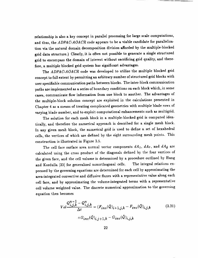
The solution for each mesh block in a multiple-blocked grid is computed iden-
tically, and therefore the numerical approach is described for a single mesh block.
In any given mesh block, the numerical grid is used to define a set of hexahedral
cells, the vertices of which are defined by the eight surrounding mesh points. This
construction is illustrated in Figure 3.5.
The cell face surface area normal vector components dAz, dAr, and dA 0 are
calculated using the cross product of the diagonals defined by the four vertices of
the given face, and the cell volume is determined by a procedure outlined by Hung
and Kordulla [33] for generalized nonorthogonal cells. The integral relations ex-
pressed by the governing equations are determined for each cell by approximating the
area-integrated convective and diffusive fluxes with a representative value along each
cell face, and by approximating the volume-integrated terms with a representative
cell volume weighted value. The discrete numerical approximation to the governing
equation then becomes
_n+l nVol'_ i'j'k - Qi,j,k
At = (Finv(Q)i+l,J, k - Finv((_)i,J, k (3.31)
+ainv( O)i,j + 1,k - ainv( d2)i,j,k
22

i-l,j-l,k- 1
I i I I I
IIIIOltlIIIUlOOUUl IIIIII1_
Grid Point
Grid Line
Hidden Grid Line
Surface Area Normal Vector
Cell Face Diagonal Vector
SS
I
I
I
i-lj-l,kS
SS
SS
_lO|OJol|se.le|| Volume V
i,j,k-I
Figure 3.5: Three-dimensional finite volume cell
i,j,k
SA
i,j-l,k
23

+ Hinv( (_ )i,j,k + l - Hinv( (_ )i,j,k
+ Fvis( (_ )i + 1,j,k - Fvis( (_ )i,j,k
+Gvis( Q )i,j + 1,k - Gvis( (_ )i,j,k
+Hvis(Q)i,j,k+ l - Hvis(Q)i,j,k)
+VolK + Di,j,k((_)
Here, i,3, k represents the local cell indices in the structured cell array, Vol is
the local cell volume, At is the calculation time interval, and Di,j, k is an artificial
numerical dissipation function which is added to the governing equations to aid nu-
merical stability, and to eliminate spurious numerical oscillations in the vicinity of
flow discontinuities such as shock waves. Following the algorithm defined by Jame-
son [35], it is convenient to store the flow variables as a representative value for the
interior of each cell, and thus the scheme is referred to as cell-centered. The discrete
convective fluxes are constructed by using a representative value of the flow variables
which is determined by an algebraic average of the values of Q in the cells lying on
either side of the local cell face. Viscous stress terms and thermal conduction terms
are constructed by applying a generalized coordinate transformation to the governing
equations as follows:
= _(z,_,0), _ = .(z,_,0), _ = _(z,r,0) (3.32)
The chain rule may then be used to expand the various derivatives in the viscous
stresses as:0 0_ 0 071 0 0( 0
Oz Ox O_ + Oz Or1 + Ox O( (3.33)
0 0_ 0 0_ 0 0_ 0Or - Or 0_ + 0--_0-'_ + 0-"_0"-_' (3.34)
0O - 0/_ 0( + 0"_ 0"'_ + 0"_ 0-'_' (3.35)
The transformed derivatives may now be easily calculated by differencing the variables
in computational space (i corresponds to the _ direction, j corresponds to the r] di-
rection, and k corresponds to the _ direction), and utilizing the appropriate identities
for the metric differences (see e.g. [32]).
24

3.5 Runge-Kutta Time Integration
The time-stepping scheme used to advance the discrete numerical representation
of the governing equations is a multistage Runge-Kutta integration. An m stage
Runge-Kutta integration for the discretized equations is expressed as:
Q1 -- Qn _ cq At[L(Qn) + D(Qn)I,
Q2 = Qn _ a2At[L(Q1) + D(Qn)I,
Q3 = Qn _ _3AtIL(Q2) + D(Qn)I,
Q4 = Qn _ (_4AtIL(Q3) + D(Qn)],
Qm = Qn _ araAt[L(Qm_l ) + D(Qn)j,
Qn+ l = Qm (3.36)
where:
L(Q) = Linv(Q)- Lvis(Q) (3.37)
For simplicity, viscous flux contributions to the discretized equations are only cal-
culated for the first stage, and the values are frozen for the remaining stages. This
reduces the overall computational effort and does not appear to significantly alter the
solution for unsteady flows (there is no difference for steady state flows). It is also
generally not necessary to recompute the added numerical dissipation terms during
each stage. In this study, three different multistage Runge-Kutta schemes (2 four-
stage schemes, and 1 five-stage scheme) were investigated. The differences between
the schemes will be described in more detail in a later section.
A linear stability analysis of the four and five-stage Runge-Kutta time-stepping
schemes utilized during this study indicate that the schemes are stable for all calcu-
lation time increments 6t which satisfy the stability criteria CFL < 2v/2 (four stage)
25

or UFL <_ 3.75 (five stage). Based on convection constraints alone, the UFL number
may be defined in a one-dimensional manner as:
AtCFL - (3.38)
In practice, the calculation time interval must also include restrictions resulting from
diffusion phenomena. The time step used in the numerical calculation results from
both convective and diffusive considerations and is calculated as:
1.0 ) (3.39)At = CFL hi + Aj + Ak + u i + uj + _,k
where the convective and diffusive coordinate wave speeds (_ and v, repsectively) are
defined as:
"_i = Vol/(V . Si + a) (3.40)
pV°12 (3.41)
vi - CAt(S2)# '
The factor CAt is a "safety factor" of sorts, which must be imposed as a result of
the limitations of the linear stability constraints for a set of equations which are truly
nonlinear. This factor was determined through numerical experimentation and is
normally chosen to be 4.0.
For steady state flow calculations, an acceleration technique known as local time
stepping is used to enhance convergence to the steady-state solution. Local time step-
ping utilizes the maximum allowable time increment at each point during the course
of the solution. While this destroys the physical nature of the transient solution, the
steady-state solution is unaffected and can be obtained in fewer iterations of the time-
stepping scheme. For unsteady flow calculations, of course, a uniform value of the
time step At must be used at every grid point to maintain the time-accuracy of the
solution. Other convergence enhancements such as implicit residual smoothing and
multigrid (described in later sections) are also applied for steady flow calculations.
26

3.6 Fluid Properties
The working fluid is assumed to be _ir acting as a perfect gas, thus the ideal gas
equation of state has been used. Fluid properties such as specific heats, specific heat
ratio, and Prandtl number are assumed to be constant. The fluid viscosity is either
specified as a constant, or derived from the Sutherland (see e.g. [32]) formula:
3
(T)_
--- C1 T + C 2(3.42)
The so-called second coefficient of viscosity _v is fixed according to:
2
Av = -_p (3.43)
The thermal conductivity is determined from the viscosity and the definition of the
Prandtl number as:
k = Cp_____p_ (3.44)Pr
3.7 Dissipation Function
In order to prevent odd-even decoupling of the numerical solution, nonphysical
oscillations near shock waves, and to obtain rapid convergence for steady state solu-
tions, artificial dissipative terms are added to the discrete numerical representation
of the governing equations. The added dissipation model is based on the combined
works of Jameson et al. [35], Martinelli [10], and Swanson et al. [36]. A blend of
fourth and second differences is used to provide a third order background dissipation
in smooth flow regions and first order dissipation near discontinuities. The discrete
equation dissipative function is given by:
2= _ _ k)Q (3.45)
The second and fourth order dissipation operators are determined by
D_Qi,j, k = V(((_)i, le2.. 1 • k )/_ Qi,j,k-t-_ z-t-_,3,
(3.46)
27

D_Qi,j,k= _Y_((Y_)i, le4. 1 -k) A_ _Y_ A_ Qi,j,k (3.47)±2 2-e_,j,
where A_ and _7_ axe forward and backward difference operators in the _ direction.
In order to avoid excessively large levels of dissipation for cells with large aspect
ratios, and to maintain the damping properties of the scheme, a variable scaling of
the dissipative terms is employed which is an extension of the two dimensional scheme
given by MaxtineUi [10]. The scaling factor is defined as a function of the spectral
radius of the Jacobian matrices associated with the _, _7, and ¢ directions and provides
a scaling mechanism for varying cell aspect ratios through the following scheme:
(5_)i+½,J,k=(X_) •.z__7,3,t_1" "q_i '-_2,j,1 :k (3.48)
The function ¢ controls the relative importance of dissipation in the three coordinate
directions as:
[ (XTl)i+½,J,k.a (A()i+½,J,k)ct)¢i+½,J,k =1 +max (((X()i+½,J,k) '(()_()i+½,J,k
The directional eigenvalue scaling functions are defined by:
( )_rl) i + ½,j, k = U.,..r 2,3,al• , ( Srt ) . ,,.v,2,.t,1: k + c( S_?) i + ½,J,k
(3.49)
(3.50)
(3.51)
(3.52)
The use of the maximum function in the definition of • is important for grids where
X_//A_ and 2_/A_ are very large and of the same order of magnitude. In this case,
if these ratios are summed rather than taking the maximum, the dissipation can
become too large, resulting in degraded solution accuracy and poor convergence•
Because three-dimensional solution grids tend to exhibit large variations in the cell
aspect ratio, there is less freedom in the choice of the parameter c_ for this scheme,
and a value of 0.5 was found to provide a robust scheme.
28

The coefficientsin the dissipationoperator usethe solution pressureasa sensor
for the presenceof shockwavesin the solution and aredefinedas:
e2i+½,J,k = _2max(ui-l,j,k'ui'j'k'ui+l,j,k'Ui+2,j,k) (3.53)
t(Pi-l,j,k - 2pi,j,k + Pi+ 1,j,k)l (3.54)ui'j'k = (Pi-l,j,k + 2pi,j,k + Pi+l,j,k)
e4'z_l,j,k = max(O, a4 _ e.2, 14 k )(3.55)
where _2, _;4 are user-defined constants. Typical values for these variables are
2= 1 _4 = __1 (3.26)2 64
The dissipation operators in the r] and _ directions are defined in a similar manner.
3.8 Implicit Residual Smoothing
The stability range of the basic time-stepping scheme can be extended using
implicit smoothing of the residuals. This technique was described by Hollanders
et al. [37] for the Lax-Wendroff scheme and later developed by Jameson [35] for
the Runge-Kutta scheme. Since an unsteady flow calculation for a given geome-
try and grid is likely to be computationaJly more expensive than a similar steady
flow calculation, it would be advantageous to utilize this acceleration technique for
time-dependent flow calculations as well. In recent calculations for two dimensional
unsteady flows, Jorgensen and Chima [38] demonstrated that a variant of the im-
plicit residual smoothing technique could be incorporated into a time-accurate ex-
plicit method to permit the use of larger calculation time increments without ad-
versely affecting the results of the unsteady calculation. The implementation of this
residual smoothing scheme reduced the CPU time for their calculation by a factor
of five. This so-called time-accurate implicit residual smoothing operator was then
also demonstrated by Rao and Delaney [39] for a similar two-dimensional unsteady
calculation. Although this "time-accurate" implicit residual smoothing scheme is not
29
developed theoretically to accurately provide the unsteady solution, it can be demon-
strated that errors introduced through this residual smoothing process are very local
in nature, and are generally not greater than the discretization error.
The standard implicit residual smoothing operator can be written as:
(1-e_ A_ V_)(1-ey/kTi Vrl)(1-ei A_ V(_)Rm= Rrn (3.57)
where the residual Rm is defined as:
At
am = am'-_-(Qm - Din), m = 1,restages (3.58)
for each of the m stages in the Runge-Kutta multistage scheme. Here Qm is the sum
of the convective and diffusive terms, Drn the total dissipation at stage m, and/_rn
the final (smoothed) residual at stage m.
The smoothing reduction is applied sequentially in each coordinate direction as:
: (1- -lnL
R***= Ai Vi)-IR m
km= (3.59)
where each of the first three steps above requires the inversion of a scalar tridiag-
onal matrix. The application of the residual smoothing operator varies with the
type of Runge-Kutta time marching scheme selected. The full four and five stage
time-marching schemes utilize residual smoothing at each stage of the Runge-Kutta
integration. The reduced four stage scheme employs residual smoothing at the second
and fourth stages only.
The use of constant coefficients (e) in the implicit treatment has proven to be
useful, even for meshes with high aspect ratio cells, provided additional support such
as enthalpy damping (see [35]) is introduced. Unfortunately, the use of enthalpy
damping, which assumes a constant total enthalpy throughout the flowfield, cannot
be used for an unsteady flow, and many steady flows where the total enthalpy may
vary. It has been shown that the need for enthalpy damping can be eliminated by using
3O

variable coefficientsin the implicit treatment which account for the variation of the
cell aspect ratio. Martinelli [10] derived a functional form for the variable coefficients
for two-dimensional flows which are functions of characteristic wave speeds. In this
study, the three-dimensional extension described by Radespiel et al. [36] is utilized,
and is expressed as:
maz 1 (3.60)eE, = I O' 4[CFLmax 1 + rnax(r_?Eri_ )] -
/
( i CFL i+max(r_ra_f) "_ )1+ max(r_r_y) J','I 'Is i-._ 1 (3.61)= o, [CFLmax
= )] - 1 (3.62)e_ max 0,-4[CFLmax 1 +
CFL represents the local value of the CFL number based on the calculation time in-
crement At, and CFLmax represents the maximum stable value of the CFL number
permitted by the unmodified scheme (normally, in practice, this is chosen as 2.5 for
a four stage scheme and 3.5 for a five stage scheme, although linear stability analy-
sis suggests that 2v/2, and 3.75 are the theoretical limits for the four and five stage
schemes, respectively). From this formulation it is obvious then that the residual
smoothing operator is only applied in those regions where the local CFL number
exceeds the stability-limited value. In this approach, the residual operator coefficient
becomes zero at points where the local CFL number is less than that required by
stability, and the influence of the smoothing is only locally applied to those regions
exceeding the stability limit. Practical experience involving unsteady flow calcula-
tions suggests that for a constant time increment, the majority of the flowfield utilizes
CFL numbers less than the stability-limited value to maintain a reasonable level of
accuracy. Local smoothing is therefore typically required only in regions of small grid
spacing, where the stability-limited time step is very small. Numerical tests both with
and without the time-accurate implicit residual smoothing operator for the flows of
interest in this study were found to produce essentially identical results, while the
time-accurate residual smoothing resulted in a decrease in CPU time by a factor of
2-3. In practice, the actual limit on the calculation CFL number were determined to
be roughly twice the values specified for CFLmax, above.
31

3.9 Turbulence Model
As a result of computer limitations regarding storage and execution speed, the
effects of turbulence are introduced through an appropriate turbulence model and
solutions are performed on a numerical grid designed to capture the macroscopic
(rather than the microscopic) behavior of the flow. A relatively standard version of
the Baldwin-Lomax [34] turbulence model was adopted for this analysis. This model
is computationally efficient, and has been successfully applied to a wide range of
geometries and flow conditions.
The effects of turbulence are introduced into the numerical scheme by utiliz-
ing the Boussinesq approximation (see e.g. [32]), resulting in an effective calculation
viscosity defined as:
#effective = Plaminar + Piurbulent (3.63)
The simulation is therefore performed using an effective viscosity which combines the
effects of the physical (laminar) viscosity and the effects of turbulence through the
turbulence model and the turbulent viscosity Pturbulent"
The Baldwin-Lomax model specifies that the turbulent viscosity be based on an
inner and outer layer of the boundary layer flow region as:
{ (Pturbulent)inner, Y <- ycrossover(3.64)
Pturbulent = (Pturbulent)outer, Y > Ycrossover
where y is the normal distance to the nearest wall, and ycrossover is the smallest
value of y at which values from the inner and outer models are equal. The inner and
outer model turbulent viscosities are defined as:
(Pturb)inner = P121wl (3.65)
(Pturb)outer = K CcppFwakeFklebY
Here, the term I is the Van Driest damping factor
l = ky(1 - e (-v+/A+))
(3.66)
(3.67)
32

w is the vorticity magnitude, Fwake is defined as:
Fwake = ymaxFmaz (3.68)
where the quantities ymaz, Fraaz are determined from the function
F(y) = y(,,'l[1 - e (-y+ /A + )] (3.69)
The term y+ is defined as
i P]_l (3.70)Y #laminar
The quantity FMA X is the maximum value of F(y) that occurs in a profile, and
YMAX is the value of y at which it occurs. The determination of FMA X and YMAX
is perhaps the most difficult aspect of this model for three-dimensional flows. The
profile of F(y) versus y can have several local maximums, and it is often difficult to
establish which values should be used. In this case, FMA X is taken as the maximum
value of F(y) between a y+ value of 350.0 and 1000.0. The function Fkleb is the
Klebanoff intermittency factor given by
Fkleb(Y ) = [1 + 5.5( CklebY)6l-1 (3.71)ymax
and the remainder of the terms are constants defined as:
A + = 26,
Ccp= 1.6,
Ckleb = 0.3,
k = 0.4,
K = 0.0168 (3.72)
In practice, the turbulent viscosity is limited such that it never exceeds 1000.0 times
the laminar viscosity.
The turbulent flow thermal conductivity term is also treated as the combination
of a laminar and turbulent quantity as-
kef fectiv e = klarninar + kturbulen t (3.73)
33
For turbulent flows, the turbulent thermal conductivity kgurbulent is determined from
a turbulent Prandtl number Prturbulen t such that
Cp#turtrul ent (3.74)Prturbulen t = kturlrulen t
The turbulent Prandtl number is normally chosen to have a value of 0.9.
In order to properly utilize this turbulence model, a fairly large number of grid
ceils must be present in the boundary layer flow region, and, perhaps of greater im-
portance, the spacing of the first grid cell off of a wall should be small enough to
accurately account for the inner "law of the wall" turbulent boundary layer profile
region. Unfortunately, this constraint is typically not satisfied due to grid-induced
problems or excessive computational costs, especially for time-dependent flow calcu-
lations. A convenient technique to suppress this problem is the use of wall functions
to replace the inner turbulent model function, and solve for the flow on a somewhat
coarser grid. The wall function technique has been successfully demonstrated [29] for
computer programs based on a numerical algorithm similar to the ADPAC-AOACR
solution scheme. Unfortunately, this technique has not been implemented or tested
for the current application. It appears that the use of wall functions is a reasonable
area for future research.
Practical applications of the Baldwin-Lomax model for three-dimensional viscous
flow must be made with the limitations of the model in mind. The Baldwin-Lomax
model was designed for the prediction of wall bounded turbulent shear layers, and is
not likely to be well suited for flows with massive separations or large vortical struc-
tures. There are, unfortunately, a number of applications for ducted and unducted
propfans where this model is likely to be invalid. This is also likely to be an area
requiring improvement in the future.
3.10 Multigrid Convergence Acceleration
Multigrid (not to be confused with a multiple blocked grid!) is a numerical so-
lution technique which attempts to accelerate the convergence of an iterative process
(such as a steady flow prediction using a time-marching scheme) by computing cor-
rections to the solution on coarser meshes and propagating these changes to the fine
34

mesh through interpolation. This operation may be recursively applied to several
coarsenings of the original mesh to effectively enhance the overall convergence. In
the present multigrid application, coarse meshes are derived from the preceding finer
mesh by eliminating every other mesh line in each coordinate direction as shown in
Figure 3.6. As a result, the number of multigrid levels (coarse mesh divisions) is
controlled by the mesh size, and, in the case of the ADPAC-AOACR code, also by
the indices of the embedded mesh boundaries (such as blade leading and trailing
edges, etc.) (see Figure 3.6). These restrictions suggest that mesh blocks should be
constructed such that the internal boundaries and overall size coincide with numbers
which are compatible with the multigrid solution procedure (i.e., the mesh size should
be 1 greater than any number which can be divided by 2 several times and remain
whole numbers: e.g. 9, 17, 33, 65 etc.)
The multigrid procedure is applied in a V-cycle as shown in Figure 3.7, whereby
the fine mesh solution is initially "injected" into the next coarser mesh, the appro-
priate forcing functions are then calculated based on the differences between the
calculated coarse mesh residual and the residual which results from a summation of
the fine mesh residuals for the coarse mesh cell, and the solution is advanced on the
coarse mesh. This sequence is repeated on each successively coarser mesh until the
coarsest mesh is reached. At this point, the correction to the solution t_n+lt'_ i,j,k- Q_,j,k )
is interpolated to the next finer mesh, a new solution is defined on that mesh, and the
interpolation of corrections is applied sequentially until the finest mesh is reached.
Following a concept suggested by Swanson et al. [36], it is sometimes desirable to
smooth the final corrections on the finest mesh to reduce the effects of oscillations
induced by the interpolation process. A constant coefficient implementation of the
implicit residual smoothing scheme described in Section 3.5 is used for this purpose.
The value of the smoothing constant is normally taken to be 0.2.
A second multigrid concept which should be discussed is the so-called "full"
multigrid startup procedure. The "full" multigrid method is used to initialize a solu-
tion by first computing the flow on a coarse mesh, performing several time-marching
iterations on that mesh (which, by the way could be multigrid iterations if succes-
sively coarser meshes are available), and then interpolating the solution at that point
to the next finer mesh, and repeating the entire process until the finest mesh level
35

MultigridAlgorithmMeshLevelDescription
FineMesh CoarseMesh CoarseMesh
LevelI Level2 Level3
Everyothermeshlineremovedto definenextmeshlevel
Gridlinesdefiningmeshboundariesandinternalboundaries(bladeleadingedges,trailingedges,etc.)
mustbeconsistentwiththemeshcoarseningprocess(cannotremovea meshlinedefiningaboundary
forthegivencoordinatedirection)
Figure 3.6: Multigrid Mesh Coarsening Strategy and Mesh Index Relation
36

Multigrid V-Cycle Strategy
--I_ Advance Solution on Current Mesh
--I_ Update Solution with Corrections
Mesh Level
!i
Solution
Injection
ii
Solution
Injection
Sample cycle shown is for
four level multigrid
Interpolate
Corrections
Interpolate
Corrections
InjectionInterpolate
Corrections
Figure 3.7: Multigrid V Cycle Strategy
37

is reached. The intent here is to generate a reasonably approximate solution on
the coarser meshes before undergoing the expense of the fine mesh multigrid cycles.
Again, the "full" multigrid technique only applies to starting up a solution.
3.11 Single Block Boundary Conditions
In this section, the various boundary conditions which are available as part of
the ADPAC-AOACR code pertaining to a single mesh block are described. Before
describing the individual boundary conditions, it may be useful to describe how the
boundary conditions are imposed in the discrete numerical solution. Finite volume so-
lution algorithms such as the ADPAC-AOA CR program typically employ the concept
of a phantom cell to impose boundary conditions on the external faces of a particular
mesh block. This concept is illustrated graphically for a 2-D mesh representation in
Figure 3.8.
A phantom cell is a fictitious neighboring cell located outside the extent of a
mesh which is utilized in the application of boundary conditions on the outer bound-
aries of a mesh block. Since flow variables cannot be directly specified at a mesh
surface in a finite volume solution (the flow variables are calculated and stored at
cell centers), the boundary data specified in the phantom cells are utilized to control
the flux condition at the cell faces of the outer boundary of the mesh block, and, in
turn, satisfy a particular boundary condition. All ADPAC-AOACR boundary con-
dition specifications provide data values for phantom cells to implement a particular
mathematical boundary condition on the mesh. Another advantage of the phantom
cell approach is that it permits unmodified application of the interior point scheme
at near boundary cells.
Inflow and exit boundary conditions are applied numerically using characteristic
theory. A one-dimensional isentropic system of equations is utilized to derive the
following characteristic equations at an axial inflow/outflow boundary:
OC-
Ot
OC +
Ot
OC-
(vz- a) - o,
. OC +
+(vz =0
(3.75)
(3.76)
38

2-D Mesh Block Phantom Cell Representation
• Grid Point
Grid Line
Mesh Block Boundary
Phantom Cell Representation
_ F qw lw
I
L_ : ,:
--- ,_ i,_
• -- ; :: •
IL \, %< ,-X'-" " -"N "
J
i
• W I W I W _W IW qV q w I w
d L • L . L . L • JL • •
l i :-- i i l I/ i l
|!
Boundary condition specifications control the
flow variables for the phantom cells adjacent to
the mesh block boundary
"Comer" phantom cells cannot be controlled
through boundary conditions, but must be updated
to accurately compute grid point averaged values
Figure 3.8: 2-D Mesh Block Phantom Cell Representation
39

where:
2a C+ 2aC- : Vz , : Vz + _ (3.77)_t-1 "7-1
For subsonic normal inflow, the upstream running invariant C- is extrapolated
to the inlet, and along with the equation of state, specified total pressure, total tem-
perature, and flow angle (used to specify the angle of attack), the flow variables at the
boundary may be determined. Inlet boundaries also require the specification of a flow
direction. This is accomplished in one of two different manners. For turbomachinery
based flow calculations, it is typical to specify a radial and circumferential (swirl)
flow angle. For external flow calculations (such as angle of attack flow analysis) a
Cartesian based flow angle is prescribed. It should be mentioned that the effective
inflow angle in this case may vary for a given block as it rotates about the axis, and
therefore the inflow angle is actually a function of circumferential position, 8.
Outflow boundaries require a specification of the exit static pressure at either the
bottom or top of the exit plane. The remaining pressures along the outflow boundary
are calculated by integrating the radial momentum equation:
Op pv_- (3.78)
Or r
In this case, the downstream running invariant C ÷ is used to update the phantom
cells at the exit boundary.
Far-field boundaries also use the characteristic technique based on whether the
local flow normal to the boundary passes into or out of the domain.
All solid surfaces (hub, cowl, airfoils) must satisfy either flow tangency for inviscid
flOW:
I7._=0 (3.79)
or no slip for viscous flows:
Vz = O, Vr = O, v 8 = rw (3.80)
In both cases, no convective flux through the boundary (an impermeable surface) is
permitted. The phantom cell velocity components are thus constructed to ensure that
4O
the cell face average velocities used in the convective flux calculation are identically
zero. The phantom cell pressure is simply extrapolated based on the boundary layer
flow concept dp/dn = 0 (although for inviscid flows a normal momentum equation is
likely to be more accurate). In the present applications, for inviscid flows, extrapo-
lation was found to be the most effective technique based on rapid convergence and
solution accuracy. The phantom cell density or temperature is imposed by assuming
either an adiabatic surface dT/dn = 0 or a specified surface temperature, which sug-
gests that the phantom cell temperature must be properly constructed to satisfy the
appropriate average temperature along the surface.
Some final comments concerning boundaries are in order at this point. Artificial
damping is applied at the block boundaries by prescribing zero dissipation flux along
block boundaries to maintain the global conservative nature of the solution for each
mesh block. Fourth order dissipation fluxes at near boundary cells are computed using
a modified one-sided differencing scheme. Implicit residual smoothing is applied at the
block boundary by imposing a zero residual gradient (i.e. (dR/dz) = 0.0) condition
at the boundary.
3.12 Multiple-Block Coupling Boundary Conditions
For the multiple-block scheme, the solution is performed on a single grid block
at a time. Special boundary conditions along block boundaries are therefore required
to provide some transport of information between blocks. This transport is provided
through one of four types of procedures. Each procedure applies to a different type
of mesh construction and flow environment, and details of each approach are given
in the paragraphs below.
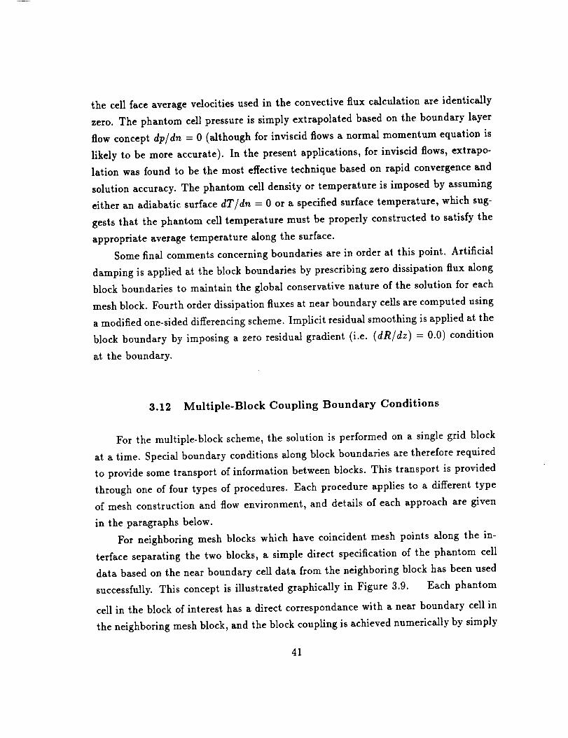
For neighboring mesh blocks which have coincident mesh points along the in-
terface separating the two blocks, a simple direct specification of the phantom cell
data based on the near boundary cell data from the neighboring block has been used
successfully. This concept is illustrated graphically in Figure 3.9. Each phantom
cell in the block of interest has a direct correspondance with a near boundary cell in
the neighboring mesh block, and the block coupling is achieved numerically by simply
41

Contiguous Mesh Block Interface
Boundary Coupling Scheme
Mesh Block Structure
Phantom cell data values for mesh block#l
are determined by corresponding near-boundary
data in mesh block #2
I I I I
Mesh Block #1' I
- --I
-- -1
-- 7
-- -1.__-__
_t---m
._t---- m
I I I I
Mesh Block #2| I [
Figure 3.9:
v
Block BoundaryMesh Line
Phantom Cell RepresentationPhantom Cell Data Path
ADPA C-A OA CR Contiguous Mesh Block Coupling Scheme
42

assigning the value of the corresponding cell in the neighboring block to the phantom
cell of the block of interest. This procedure essentially duplicates the interior point
solution scheme for the near boundary cells, and uniformly enforces the conservation
principles implied by the governing equations.
For mesh block interfaces which do not have coincident points, but which define
essentially the same surface, it is necessary to perform some type of interpolation
to determine representative values for the block-specific phantom cells absed on the
near boundary interface data from the neighboring mesh block. A relatively simple
interpolation scheme based on an electrical resistance analogy was developed for this
purpose_ and is illustrated graphically for a non-contiguous mesh block interface as
shown in Figure 3.10. To determine the phantom cell data for a non-contiguous
mesh block interface, the center of the nearest cell face for the particular phantom cell
is determined by averaging the coordinates of the four mesh points which determine
the cell face. A search is then performed in the neighboring mesh block along the
same interface to determine the cell face whose center lies closest to the phantom cell
face center of interest. It is assumed that both mesh blocks share a common surface
at the interface of interest, in spite of the fact that this surface is defined by different
points. This assumption thus requires that the block boundaries do not overlap, and
that the physical extent of the boundaries are approximately equal. Once the nearest
cell in the neighboring mesh block has been located, the nearest set of four cells
in the neighboring mesh is determined_ and an electrical circuit analogy is used to
interpolate the phantom cell boundary data from the four cells of neighboring mesh
block data. The circuit analogy simply sets a resistance for each path of neighboring
cell data to the phantom cell center based on the physical distance between the centers
of each cell face (again, this concept is illustrated in Figure 3.10. The four neighboring
cell near boundary data are then treated as voltages, and the phantom cell data are
determined by calculating the appropriate "voltage '_ potential at the phantom cell
face center based on the neighboring cell face center data and the resistance along
each path. This scheme has the advantages of being simple to program, is extremely
stable, and identically duplicates the contiguous mesh block interface phantom cell
representation_ described above, for interfaces which have contiguous mesh points.
The disadvantages of this approach are that the interpolation is essentially linear,
43

Non-Contiguous Mesh Block Interface
Boundary Coupling Scheme
Mesh Block Interface Structure
A
..
.. 0"
•
"•''•.!,...°° °
Mesh Block #1 Grid Line_
........................ Mesh Block #2 Grid Lines
Mesh Block #1 Phantom Cell of Interest
°. ° o ° o_°
°'...°...°
.°°,
?•°'°-.°°°°°°.
°-
o°°°,°. ."
''7-°..,..
...... ....(........-,.•.
\
O
0
Mesh Block #1 Phantom Cell Face Center
Mesh Block #2 Boundary Cell Face Center
D
Figure 3.10:
Electrical Circuit Analogy
A
Resistance Element Proportional to Spacing
B
C
ADPA C-A OA CR Non-Contiguous Mesh Block Coupling Scheme
44

and that the scheme is not uniformly conservative, and is thus subject to errors is
mass, momentum, and energy conservation. These sources of error scale roughly with
the mesh spacing, and therefore, the finer the mesh, the lower the impact these errors
have on the overall solution.
The third type of mesh block interface boundary patching scheme relates to
steady flow calculations involving turbomachinery components with multiple blade
rows, or to a lesser extent, steady flow calculations involving mesh systems with differ-
ing circumferential extents. This approach is a technique for the prediction of steady
flow through multistage turbomachinery based on the mixing plane concept. A mixing
plane is an arbitrarily imposed boundary inserted between adjacent blade rows across
which the flow is "mixed out" circumferentially. This circumferential mixing approx-
imates the time-averaged condition at the mixing plane and allows the aerodynamic
solution for each blade passage to be performed in a steady flow environment. The
mixing plane concept was recently applied to realistic turbofan engine configurations
by Dawes [6]. Flow variables on either side of the mixing plane are circumferentially
averaged and passed to the neighboring blade row as a means of smearing out the
circumferential nonuniformities resulting from dissimilar blade counts. The mixing
plane concept is a cost-effective approach computationally because the flow is steady,
and the individual blade passage domains are limited to a near-blade region. Unfortu-
nately, the accuracy of this approach is clearly questionable under some circumstances
because of the placement of the mixing plane and the loss of spatial information re-
sulting from the circumferential averaging operator. Numerically, then, the mesh
points in two adjacent blocks at a mixing plane interface must have identical axial
and radial coordinates. This permits specifying the circumferential distribution of
phantom cells in one block as the circumferential average of the near boundary cell
data from the adjacent block. This concept is illustrated graphically in Figure 3.11.
The individual primitive flow variables are each circumferentially averaged, and used
directly in the phantom cell data specification. Attempts to use several of the more
complex mixing analyses based on the circumferentially averaged flow data, or the
use of characteristic-based boundary specification based on the flow data were both
subject to numerical instabilities under particular circumstances, and therefore, the
direct specification method is used instead.
45

Mixing Plane Concept Mesh Block
Boundary Coupling Scheme
!
!Geometry and Mesh Block Structure
I!
Mesh Block #1 Grid LinesMesh Block #2 Grid Lines
Mixing Plane Interface
k #2
Circumferential average of near-boundar3,
data in Mesh Block #2 is applied uniformly,
across the circumferential distribution of
phantom cells in Mesh Block #1
Figure 3.11:
O
ADPAC-AOAUR Circumferential Averaging (Mixing Plane)
Block Coupling Scheme for Multiple Blade Row Calculations
46
Mesh

The fourth type of mesh block interfaceboundary patching scheme relatesto
time-dependent calculationsinvolvingrelativemotion between adjacent mesh blocks.
In this case, the mesh interfaceis essentiallynoncontiguous, and the relativeposi-
tion between mesh cellsis changing in time. This type of boundary scheme isused
for the predictionof rotor/statorinteractionfor multiple blade row turbomachines.
This type of interface is complicated by the fact that the interface may be defined
by different mesh blocks at different times based on the degree of motion between
the adjacent mesh blocks. For example, if a calculation for a single stage compressor
involves 3 passages of the upstream blade row, and four passages of the downstream
blade row, then it is obvious that at some point during the calculation, each of the
three mesh blocks in the upstream blade row representation will at some time have
to communicate with each of the four mesh blocks in the downstream blade row rep-
resentation. The specific mesh block in the communication path is determined by the
degree of rotation in both the upstream and downstream blade rows, and is inher-
ently time dependent. This task is simplified considerably by requiring that the mesh
points in each block along the interface have constant axial and radial coordinates.
This simplification reduces the overall problem to a time-space interpolation in the
circumferential direction only (see Figure 3.12).
With this simplification, it is possible to simply define the interpolation data by
resolving the relative position between the mesh blocks, extracting the near bound-
ary data values from the neighboring mesh blocks, and interpolating for the phantom
cell data value based on the current circumferential position of the phantom cell face
center relative to the neighboring interpolant data arrays. Without modification, this
scheme is nonconservative and can result in spurious errors in mass, momentum, and
energy conservation across the mesh block interface. In order to rectify this problem,
a modified interpolation scheme was tested which attempted to enforce global conser-
vation of the interpolated data across each circumferential interpolation "slice" of the
mesh. This restriction was enforced by globally summing the interpolated values for
each circumferential interpolation and modifying the summation to satisfy the global
conservation defined by the interpolant data. The individual interpolated phantom
cell values were then uniformly modified to reflect the global conservation correction.
Numerical experiments with this scheme compared to the unmodified scheme were
47
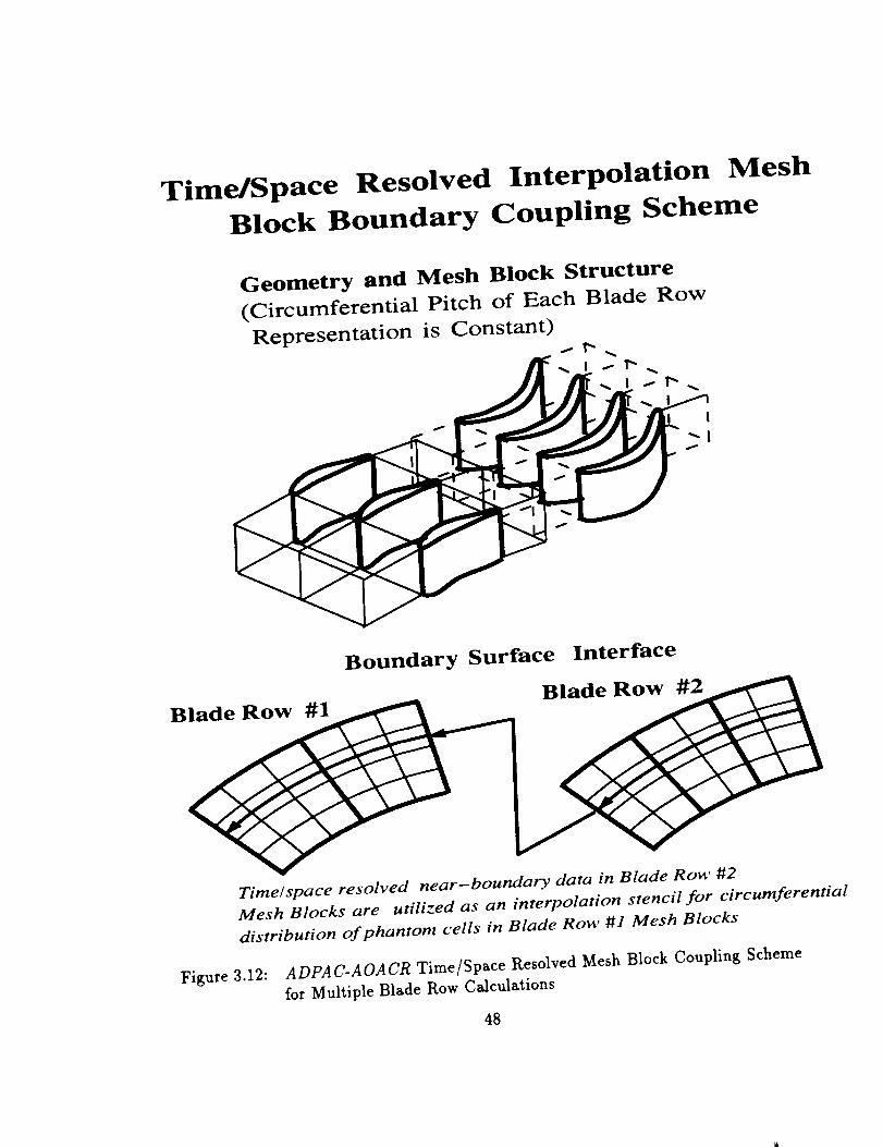
Time/Space Resolved Interpolation Mesh
Block Boundary Coupling Scheme
Geometry and Mesh Block Structure
(Circumferential Pitch of Each Blade Row
Representation is Constant)
I
Blade Row #1
Boundary Surface Interface
Blade Row #2
Time�space resolved near-boundary data in Blade Row #2
Mesh Blocks are utilized as an interpolation stencil for circumferential
distribution of phantom cells in Blade Row #1 Mesh Blocks
Figure 3.12: ADPAC-AOACR Time/Space Resolved Mesh Block Coupling Scheme
for Multiple Blade Row Calculations
48

virtually identical, and it was not possible to draw any hard conclusions regarding the
advantages of one scheme over another. Following this test, the correction scheme was
eliminated for simplicity. The effects of conservation across block interface boundaries
is likely to be a debatable issue; however, there is considerable numerical evidence
available which suggest that solution accuracy (for the types of calculations consid-
ered in this study) is not significantly influenced by non-conservative interpolation
schemes ( [12], [39]) and that supposed conservative interface coupling schemes [13]
do not necessarily ensure conservation when used with numerical schemes which are
not conservative in time.
3.13 Solution Procedure
The overall solution procedure begins by defining a set of initial data, and ad-
vancing the solution from that point forward in time until the desired solution (steady
state, time-periodic, or finite time interval) has been reached. Initial data is normally
specified as a uniform flow, or may be read in as a "restart" of a previous existing so-
lution. Normally, for steady flow calculations, the "full" multigrid startup procedure
is utilized to accelerate convergence by initializing the solution on a coarse mesh be-
fore incurring the expense of fine mesh iterations. Steady state solutions are deemed
converged when the average residual R has been reduced by a factor of 10 -3, or
when the residual has ceased to be reduced. It is possible that for some steady flow
calculations, the solution is truly unsteady (i.e. - vortex shedding behind a circular
cylinder) and in these cases the residual may not be reduced beyond a certain limit.
For time-dependent flow simulations, it has been found that it is often desirable
to first initialize the solution in a steady flow manner using mixing planes or other
time-averaged boundary condition procedures to define a reasonable approximation to
the time-averaged flow before proceeding with the time-accurate iteration procedure.
The unsteady solution may then be advanced in time with a uniformly specified time
step, until a time-periodic solution is achieved. The amount of time required to reach
a time-periodic solution is typically highly case dependent, and such solutions must
be monitored closely to determine when the solution is satisfactory.
Some comments are in order to explain the solution procedure for high speed
49

rotors, many of which are illustrated in the results section in this report. It has been
found that solutions for high speed compressor rotors typically require exit static
pressure in excess of the inlet total pressure. As a result, it is often not possible to
obtain an immediate solution under the desired operating condition because of the
potential for reversed flow at an exit boundary which results from the relatively large
exit static pressure. To overcome this problem, the following procedure has been
implemented to obtain high speed rotor flowfield solutions. Typically, the solution is
started using an exit static pressure which is lower than the inlet total pressure. For
example, for a fan rotor with a design exit static to inlet total pressure ratio of 1.13,
the solution may be started with an exit static to inlet total pressure ratio of 0.95. The
resulting solution typically chokes the flow in the blade passage and sets up a shock
system which is consistent with the choked flowfield. Once this flow is established,
the exit static pressure may be raised incrementally, and the solution restarted several
times until the desired exit static pressure ratio is reached. It should be emphasized
that the increases in back pressure must be done conservatively to avoid prematurely
stalling the blade passage.
5O

4. RESULTS
In this chapter, numerical results from the ADPAC-AOACR 3D Euler/Navier-
Stokes code are presented and compared with existing data to demonstrate and verify
the accuracy of the analysis. The results are primarily based on applications involv-
ing ducted and unducted fans with multiple blade rows; however, several additional
calculations are presented to demonstrate the versatility of the code.
Steady flow predictions involving turbomachinery geometries are presented first,
followed by several calculations of time-dependent flowfields involving multiple blade
row turbomachines.
4.1 2-D Compressor Cavity Flow (Steady Flow)
In light of the recent addition of the two-dimensional block solution capability
in the ADPAC-AOACR analysis code, a two-dimensional test demonstration for a
complex flow is appropriate. One such flow of interest to turbomachinery designers
is the flow in a compressor hub cavity for compressors which employ inner banded
stators. The exact characteristics of the leakage flow through the cavity and the
resulting interplay between the leakage flow and the primary gas flow are not com-
pletely understood. As such, inner banded stator seal design is currently an area of
concentrated investigation for high performance gas turbine engines.
The ADPAC-AOACR analysis was applied to predict the two-dimensional flow
in an inner-banded stator hub cavity design considered for an advanced compressor
design at Allison. This geometry, and the 149x61 mesh system used in the analysis
are illustrated in Figure 4.1. This complex mesh system is actually rectangular in
computational space, and the application of the appropriate boundary conditions is a
trivial matter for the ADPAC-AOACR analysis. The time-marching calculation was
51

Figure 4.1: Inner Banded Stator Cavity Geometry and ADPAC-AOACR 2-D Mesh
System
advanced with a CFL number of 5, utilized 3 levels of multigrid, and employed the
full multigrid startup procedure. The residual convergence history resulting from this
calculation is given in Figure 4.2. The full multigrid startup procedure consisted of
200 iterations on each of the 2 coarse mesh levels, followed by 100 fine mesh iterations.
The overall convergence for this case was excellent, with the average residual reduced
a full four orders of magnitude in only 100 fine mesh iterations.
The predicted steady flow velocity vector pattern for this flow is given in Fig-
ure 4.3. It should be noted that the flow in the cavity is from left to right in this
orientation. The flow consists of a complex pattern of recirculating vortices, coupled
with the high speed, high loss flow through the knife seals. It is particularly interesting
to note the standing vortices at the inlet and exit of the cavity fl0wpath. Although
no experimental data were available to verify these results, the predicted 2-D flow
was in good agreement with a similar 3-D flow prediction from the ADPAC-AOACR
analysis, and a similar 2-D flow predictions based on a separate 2-D Navier-Stokes
code.
52

Compressor Hub Cavity - ADPAC 2-D Predicti
e_o
.2
0
-2
-8
-10
I• °, ..... °°°o ......... o ...... .•°,°.•_°oo°.,°._ ............... -,.o°,°o,,°° .....
..................................::\_<21................................,,% •
...... Convergence ................ .""Max Residual
.... Avg Residual
0 100 200 3()0 400 500
Iteration Number
Figure 4.2: ADPAC-AOACR Full Multigrid Convergence
Banded Stator Cavity Flow Calculation
53
History for 2-D
i
Inner

Figure 4.3: ADPAC-AOACR Predicted Velocity Vectors for 2-D Inner Banded Sta-
tor Cavity Flow Analysis
4.2 Model Counterrotating Propfan (Steady Flow)
The first results presented are for a model counterrotating propfan geometry.
Geometric and aerodynamic design parameters for the model counterrotating pro-
peller are given in Figure 4.4. The calculations presented here were based on a cruise
condition with a flight Mach number of 0.72, and advance ratio of 3.14. The forward
and rearward blade setting angles were 57.4 and 60.0 degrees, respectively. Steady
flow performance predictions were obtained for this case by solving the Navier-Stokes
equations with the inter-blade row mixing plane concept described in Section 3.2.
The grid therefore consists of two blocks (one for each blade row), divided by the
mixing plane approximately midway between the two blade rows. Our experience sug-
gests that propfan airfoils are sufficiently flexible that in order to accurately capture
aerodynamic performance, it is necessary to perform coupled structural/aerodynamic
analyses to deduce the airfoil shape under the desired operating conditions. For the
purposes of this demonstration, the individual mesh blocks were generated based on
an assumed fixed running airfoil shape.
54

It should be noted that this grid system corresponds to standard configuration
#7 as described in the ADPAC-AOACR Computer Program Users Manual [9]. The
grid block sizes were 65x49x33 and 57x49x33, respectively. An illustration of the
mesh system is given in Figure 4.5. The calculations presented here are essentially
for demonstration purposes only. In practice, the exit boundary should probably be
extended farther downstream to obtain best results.
Calculations for this geometry utilized 3 levels of multigrid, and employed the
full multigrid startup procedure. A total of 100 iterations were performed on each of
the coarse mesh levels during the full multigrid startup, followed by 200 iterations of
the fine mesh solver. The CFL number was fixed at 5.0, and the modified four stage
time-marching algorithm was employed. An illustration of the convergence history
for this case is given in Figure 4.6.
The overall convergence of the multigrid procedure was observed to be quite
rapid, requiring only 200 fine mesh iterations to achieve a 3 order reduction of the av-
erage solution residual (error). An illustration of the predicted surface static pressure
contours and radial blade-to-blade static pressure contours are given in Figure 4.7.
The blade to blade static pressure contours clearly illustrate the tip vortex flow near
the suction side of each blade. No leading edge vortex was observed in the predictions
for either blade row under this operating condition, which appears to be supported
by experimental evidence. The overall predicted power coefficient for this case was
2.05 which is in good agreement with the design value of 2.035.
Two images are presented in Figures 4.8 and 4.9 to illustrate the effectiveness
of the mixing plane boundary patching procedure for this type of flow. Figure 4.8
illustrates predicted absolute Mach number contours for the axisymmetric averaged
flowfield. The blade boundaries and location of the mixing plane are outlined. The
corresponding axisymmetric averaged flow static pressure contours are given in Fig-
ure 4.9. Both sets of contours display a smooth transition across the mixing plane
and display no noticeable abnormalities as a result of the mixing plane assumption.
Another plot, given on Figure 4.10, illustrates the circumferential blade to blade
static pressure contours at midspan for the mixing plane calculation. The mesh block
boundaries are outlined, and the mixing plane boundary is visible between the blade
rows. Naturally, the contours do not mate at the mixing plane boundary because
55

Mesh Block Structure:
1 Mesh Block/Blade Row (2 Mesh Blocks Total)
Mixing Plane Approximately Midway BetweenBlade Rows
Number of Blades in Forward Row: 5
Number of Blades in Rearward Row: 5
Design Flight Mach Number: 0.72
Design Power Coefficient 2.035
Design Advance Ratio: 2.94
Design Tip Speed: 750 ft/s
Power Loading/D**2: 37.15
Other Design Information:
55%/45% Torque Split (Front/Rear)
Tractor Configuration
Swept Blade Design
Figure 4.4: Model Counterrotating Propfan Model Geometric and Aerodynamic De-
sign Parameters
56

I
Figure 4.5: ADPAC-AOACR Two-Block Mesh System for Steady Flow Analysis of
Model Counterrotating Propfan
57
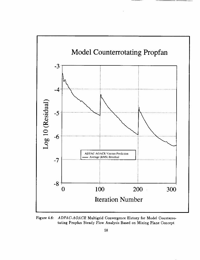
Model Counterrotating Propfan
o_ml
0
0
....................................... | .......
-7
-8
ADPAC-AOACR Viscous Prediction
Average (RMS) Residual
0 100 200 300
Iteration Number
Figure 4.6: ADPA C-AOA CR Multigrid Convergence History for Model Counterro-
rating Propfan Steady Flow Analysis Based on Mixing Plane Concept
58

Figure 4.7: ADPAC-AOACR Predicted Steady Surface Static Pressure Countoursand Post Rotor Static Pressure Contours for Model Counterrotating
Prop fan59
ORIG!r, WkL r,,,,_l.-r) m r ,-,_.COLOR r HOTcGRAPH


of the circumferential averaging procedure. It is apparent, however, that the mixing
plane does not unduly distort the flowfield contours in the vicinty of either blade row.
This calculation clearly demonstrates one application which can benefit from
the accuracy and cost-effectiveness of the mixing plane approach. Future studies
concentrating on defining the limits (in terms of interblade row spacing) would be
helpful to define the geometric regime where the mixing plane assumption is valid.
4.3 NASA 1.15 Pressure Ratio Fan (Steady Flow)
In this section, calculations are presented for the viscous flow through a 1.15
pressure ratio fan stage originally tested by NASA [42]-[47] and utilized extensively
under this contract for analysis [21],[7]. Descriptions of the geometry and design
parameters for the NASA 1.15 pressure ratio fan are given in Fig. 4.11.
The NASA 1.15 pressure ratio fan is representative of a 25:1 bypass ratio tur-
bofan engine fan stage, and therefore closely approximates the ducted propfan con-
cept propulsion system. Several steady flow calculations were performed to permit a
comparison of predicted results with the high speed experimental data published in
aef. [42].
A meridional view of the geometry and steady flow grid system are given in
Fig. 4.12.
The steady flow calculations for this geometry were performed using the mixing
plane inter-blade row model between the fan rotor and stator. It should be noted that
this grid system corresponds to standard configuration #8 described in the ADPA C-
AOACR Computer Program Users Manual (see [9]). The mesh system, illustrated in
Figure 4.12, consists of 4 mesh blocks, two each associated with the rotor and the
stator, respectively. The overall mesh block sizes were 89x37x33, 89x25x33, 81x37x33,
and 81x25x33. The rotor was represented by 33 points in the radial direction, result-
ing in 5 points to define the clearance region above the rotor tip. Calculations are
presented here for a flight Mach number of 0.75, and a fan rotational speed of 9167
rpm (100% speed). The calculation utilized 3 levels of multigrid and employed the
full multigrid startup procedure. A total of 100 iterations were performed on each of
60


Figure 4.8: ADPAC-AOACR Predicted Steady Axisymmetric Averaged Mach Num-ber Contours for Model Counterrotating Propfan
61


\
\
\,L
\
Figure 4.9: ADPA C-A OA OR Predicted Steady Axisymmetric Averaged Static Pres-
sure Contours for Model Counterrotating Propfan
62


Figure4.10: ADPAC-AOACR Predicted Steady Circumferential Blade-to-Blade
Static Pressure Contours for Model Counterrotating Propfan
63


Dorsal Pylon
XH
D
LXFC-
-XOA--
(dimensions in cm)
Figure 4.11:
l*
NASA 1.15 Pressure Ratio Fan Geometry and Design Parameters
64


Figure 4.12: ADPAC-AOACR Four Block Mesh System for NASA 1.15 Pressure
Ratio Fan
65

the coarse mesh levels during the full multigrid startup, foUowed by 300 iterations of
the fine mesh solver.
The overall convergence of the multigrid procedure was very good for this calcu-
lation, in spite of the added complexity of the multiple block discretization and the
mixing plane coupling scheme. Predicted axisymmetric averaged flow contours for
absolute Mach number and static pressure are illustrated on Figures 4.13 and 4.14,
respectively.
The cowl, spinner, blades, and mixing planes are outlined on both figures. The
axisymmetric flow displays a smooth transition across the mixing plane, although
this feature was certainly not unexpected considering the axial separation between
the blade rows for this case.
A comparison of the predicted stator exit radial total pressure distribution with
experimental data and numerical data obtained with the average-passage formulation
developed under Task I of this contract [21] is presented in Figure 4.15. The inviscid
prediction using the HPRO3D developed under Task 1 clearly overpredicts the total
pressure ratio at the nozzle entrance as a result of the lack of viscous losses. The
present prediction shows good agreement across the radial span excepet near the
hub, where the ADPAC-AOACR results clearly underpredict the total pressure rise
through the machine. This discrepency is thought to be due to numerically generated
losses as a result of poor grid refinement near the spinner leading edge. These losses
are ultimately convected downstream and end up showing up along the hub at the
nozzle entrance. An illustration of the three-dimensional fiowfield for this case is
given in Figure 4.16. This figure displays predicted surface static pressure contours
for a 3-D representation of the entire fan geometry, with a portion of the fan cowl cut
away to expose the inner fan detail.
Additional calculations for this geometry were performed under various flow con-
ditions (although the results will not be reported in detail here) including a supersonic
flight test case at a freestream Mach number of 2.5. (In this case, the supersonic flow
condition was generated by specifying an initial freestream Mach number of 2.5, and
simply neglecting the application of any boundary condition at the mesh inlet, im-
plying that the initial values are never modified, which provides a physically realistic
supersonic inflow boundary treatment.) This case is mentioned only as an example
66

//
/
it
{
.>;.;] : z
,5 kl- "
--.. / \"_, Z
I ".. / \
__---->\i .................._,.<%_l.J_. ................... : + .
I
II ,
Figure 4.13: ADPAC-AOACR Predicted Axisymmetric Averaged Flow AbsoluteMach Number Contours for NASA 1.15 Presure Ratio Fan
67
ORIG ..... ,:,.....
COLOR PH,OiOGRApH


\\
\\
\\
,//
/
\\ \ i </<" " ",.
\ J / ", < ,
• \ ,_ . ., \ , • \ ) /
. " , / / / f
Figure 4.14: ADPAC-AOACR Predicted Axisymmetric Averaged Flow Static Pres-sure Contours for NASA 1.15 Presure Ratio Fan
68


NASA 1.15 Pressure Ratio Fan, Math Number=0.75
Nozzle Inlet Radial Total Pressure Distribution
1.20 --
1.00 --
0.80
tr-
y 0.60 --¢-
Q.O3
.w"o
£Z:
0.40 --
0.20
1.00
Figure 4.15:
n
n
rm ,I
• I
r'T-tI
rm
rm
!
I
I
I
I
f
#
II
I#
II
I"1-1/
oBB•¢
%=/=
I I I I1.20 1.40 1.60 1.80
Total Pressure Ratio (P/P(Infinity))
Comparison of Predicted and Experimental Stator Exit Radial To-
tal Pressure Ratio Distribution for NASA 1.15 Pressure Ratio Fan
(M=0.75) 69
I2.00


Figure 4.16: ADPAC-AOACR Predicted 3-D Surface Static Pressure Contours forNASA 1.15 Pressure Ratio Fan (M=0.75)
7O
OP,_G ..... r,,, .. -
COLOR p.:.-iOiOG RAPH


of the flexibility of the code for solving a wide variety of flow problems. In most cases
tested, the multigrid procedure rapidly converged to a steady state solution (3 order
of magnitude reduction in the average fine mesh residual) in less than 300 fine mesh
iterations.
4.4 GMA3007 Fan Section (Steady Flow)
Steady flow verification of the ADPAC-AOACR code was also performed for an
advanced turbofan engine fan rotor geometry taken from the Allison GMA3007 tur-
bofan engine. The Allison GMA3007 is a 5:1 bypass ratio turbofan engine which
produces 7,000 pounds of thrust. The fan section geometry considered consists of
three blade rows including the fan rotor, bypass stator, and core stator. The flow
is complicated by the presence of the core flow splitter, and the fact that there are
multiple exits (bypass flow, core flow) for which proper boundary data must be spec-
ified. An outline of the GMA3007 fan section geometry is given in Figure 4.17. This
domain was arbitrarily decomposed into three mesh blocks, as shown in Figure 4.17.
The individual mesh blocks correspond to one of the three blade rows in the fan
section. For steady flow analysis, the mixing plane concept described in Section 3.2
was invoked, and therefore the circumferenti_d pitch of each mesh block corresponds
to the periodic spacing of the included blade row. In addition to the axial placement
of the mixing planes between blade rows, the mesh system was designed to illustrate
a radial mixing plane which separates the mesh blocks for the bypass stator (#2) and
the core stator (#3) just upstream of the core flow splitter. Obviously, proper place-
ment of the mesh block boundaries could have removed the need for this interface,
but a demonstration of the radial mixing plane was thought to be justified in light
of future tasks under the current contract which will utilize this type of boundary in
more detail.
The actual mesh system is detailed in Figures 4.18 and 4.19. The grid block sizes
were 85x73x29, 101x33x29, and 101x41x29, respectively. The grid was constructed
by using the program TIGG3D, and special care was taken to maintain a reasonable
clustering of mesh points near solid boundaries to resolve the viscous shear layers, and
71

Mesh # 1 (85x73x29)
Mesh Block Structure
Mesh #3 (101x41x29)
Fan
Rotor(24)
Bypass Stato
Core Stator
Mixing Mesh #2 (101x33x29
Figure 4.17: Allison GMA3007 Fan Section Geometry
72

Figure 4.18: Axisymmetric Detail of ADPAC-AOA CR Three-Block Mesh System forAllison GMA3007 Fan Section
to maintain grid indices which were compatible with the multigrid solution technique.
The fan rotor includes a tip clearance region which was discretized with 9 points
radially to resolve the tip clearance flow.
The numerical solution was performed using 3 levels for multigrid and was ini-
tiated with the full multigrid startup procedure. As is typical for high speed rotor
flowfield calculations, the solution must be initiated at a back pressure which is lower
than the intended solution back pressure. The usual procedure is to slowly raise the
back pressure to the desired setting by restarting the calculation a number of times
from a previous run. This procedure prevents excessive shock motion while setting
up the flowfield which can prematurely cause the flowfield to stall. In this case, since
there are multiple domain exit regions, following the recommended startup procedure
is even more important to eliminate large oscillations in the flow split between the
core and bypass ducts.
73

Figure 4.19: Circumferential Detail of ADPAC-AOACR Three-Block Mesh Systemfor Allison GMA3007 Fan Section
Following the startup procedure described above, a design point (100% speed)
solution was achieved in approximately 1500 fine mesh iterations. Experimental data
were available at several points throughout this flow.
Figure 4.20 illustrates a comparison of the pre'dicted and experimental fan ro-
tor exit radial total pressure ratio distribution taken approximately one half chord
downstream of the rotor. Predicted results from several other calculations for this
geometry are also included on this Figure to illustrate the accuracy of the ADPAC-
A OA CR code compared with other analyses. It should be mentioned that some slight
differences in operating condition (mass flow rate, etc.) existed between the various
predictions displayed on this figure, which is at least partially responsible for the
differences in the results. The ADPA C-A OA CR results are clearly in good agreement
with the experimental data at this point, and is at least as accurate as any other
analysis which has been tested for this geometry to date. An interesting observation
from this result is that the ADPAC-AOACR prediction is in good agreement with
the ADPAC-APES code, which was also developed under this contract, and which
utilizes the more complicated average-passage solution scheme for multiple blade row
74

GMA 3007 Fan Section - Near Design Condition
Total Pressure Ratio: Inlet to Post-Rotor Exit
.2..'
iv
c-
o.O9
1.00- --
0.90 --
0.80 --
0.70 --
0.60 --
0.50 --
0.40 --
0.30 --
0.20 --
0.10--
I-1:3 Experimental Data •
ADPAC-APES Inviscid Prediction [Ref. 8]
I
...... ADPAC-APES Viscous Prediction [Ref. 8]
..... Allison 3-D Viscous Prediction [Ref. 1]Dawes Code Viscous Prediction [Ref. 6]ADPAC-AOACR Viscous Prediction
I I I0.80 0.85 0.90 0.95 1.00 1.05 1.10
Total Pressure Ratio (Pt(Iocal)/Pt(Design))
I I1.15 1.20
0.00 I I I I
Figure 4.20: Comparison of Predicted and Experimental Radial Total Pressure Ra-
tio Distributions Downstream of Fan Rotor for Allison GMA3007 Fan
Section75

.J_
1.20 --
1.10 --
0.90 -
0.80 --
0.70 --
"_ 0.60 --
==_. 0.50 --
.-.-" 0.40 --ccOa.
O3
0.30 --
0.20 --
0.10--
GMA 3007 Fan Section - Near Design Condition
Total Pressure�Temperature Ratios at Bypass Stator Leading Edge
Figure 4.21:
l 13 Experimental Test Data-> Pres_m_-'"-"__
& Experimental Test Data -> Temperature II...... ADPAC-APES Prediction (Ref. [8]) --> Pressure II..... ADPAC-APES Prediction (Ref. [8]) -> Temperature II------ ADPAC-AOACR Prediction -> Pressure II
_iction -> Temperature
_.=..:.:-- .................... _e> . •"--_ _._
• /_\ ",J
/
o*
l,
,,&I.
;.i
J
!| |
o
I'
• g
I& /.';. I:
i a _,*!im
A_
y,,,"
/,° I
.... _--_ ;L
I"id
/ :/ .
/ ./ .
I:O
i.i.I" 0
I"
/,"[]
I- I- I I I I I I0.80 0.85 0.90 0.95 1.00 1.05 1.10 1.15 1.20
Total Pressure/Temperature Ratio (Pt/Pt(Design)), (Tt/Tt(Desic
Comparison of Predicted and Experimental Radial Total Pressure and
Total Temperature Ratio Distributionsat Bypass Vane Leading Edge
for Allison GMA3007 Fan Section76

Figure 4.22: PredictedAxisymmetric-AveragedStatic PressureContoursfor AllisonGMA3007Fan Section
77
%. , ._


Figure 4.23: Predicted Surface Static Pressure Contours for Allison GMA3007 Fan
Section
78
• • • .)
• . • ..... -m ", _'LJ
COLO__ i::i__:'Ji_:_r_l' '_"


turbomachines. One would expect that the average-passage equation system provides
a more accurate model for steady flow analysis of interblade row interactions than
the simpler mixing plane concept; however, the large axial spacing between blade
rows in this turbomachinery geometry suggests that this advantage is likely to be less
influential, and the good agreement between predictions supports this observation. A
similar comparison of the predicted and experimental bypass stator leading edge ra-
dial total pressure and total temperature distributions is given on Figure 4.21. Once
again, the ADPA C-AOA CR results are in good agreement with the average passage
prediction for this geometry.
An illustration of the predicted axisymmetric-averaged static pressure contours
for this calculation are presented in Figure 4.22. The stagnation region around the
core flow splitter is clearly defined, and it is clear that there is some slight negative
incidence in the vicinity of the splitter leading edge. This incidence is clearly depen-
dent on the exit pressure chosen for both the core flow and bypass flow domains, and
our experience has been that the solution is relatively sensitive to small changes in
either specification.
Finally, to illustrate the three-dimensional nature of this fiowfield, an illustra-
tion of the predicted static pressure contours for a complete representation of the
GMA3007 fan section is given in Figure 4.23. The contours clearly display the rotor
shock location, and the flowfields associated with the core and bypass stators. The
complexity of this figure demonstrates the capability of the ADPAC-AOACR code to
analyze complex, realistic turbofan engine flowfields.
4.5 Oscillating Flat Plate Cascade (Unsteady Flow)
Before proceeding with a discussion of time-dependent predictions for multi-
ple blade row turbomachines, a demonstration of the time-accuracy of the ADPAC-
AOACR solution procedure seems appropriate. A numerical study was performed
involving the time-dependent flowfield about an oscillating flat plate cascade. This
calculation serves to further verify the time accuracy of the ADPAC-AOACR code,
and can provide some insight into the possibility of utilizing nonlinear time-marching
numerical solution techniques for the prediction of blade motion induced acoustic
79

phenomena in turbomachinery components. A detailed discussion of calculations of
this type was recently presented by Huff [45], and these results were used to guide
the present calculations.
The calculation was based on a zero stagger flat plate cascade with a pitch to
chord ratio of 1.0. The cascade motion was represented by a pitchwise plunging
harmonic oscillation. This configuration is illustrated in Figure 4.24. The cascade
motion was programmed into the ADPA C-A OA CR code by temporarily incorporating
a time-varying blade rotation term. The solution was initiated from a steady, uniform
flowfield, and advanced in time under the influence of the harmonic blade motion,
until a time-periodic solution was achieved. Calculations were performed on both a
fine and coarse mesh system for a reduced frequency of 4.0 (defined as
_C
k - (4.1)(2V 1 )
where k is the reduced frequency, _v is the harmonic oscillation frequency, c is the
flat plate chord, and V 1 is the freestream velocity. The freestream flow Mach number
was 0.5. The amplitude of the cascade vibration was 0.1% of the blade chord. The
mesh systems were actually based on a 2-D grid system generated by personnel at
the NASA-Lewis Research Center, which was stacked radially to construct a 3-D
mesh system. The 3-D mesh system was constructed with a hub to tip ratio of
0.996 and a radius to chord ratio of 100.0, which were believed to be sufficient to
minimize radial flow gradients and non-planar flow features resulting from the use of
a cylindrical coordinate system.. The coarse grid was decomposed from the fine grid
by ehminating every other grid line. An illustration of the blade-to-blade component
of both mesh systems is given in Figure 4.25.
The fine mesh size was 121x5x41, while the coarse mesh was 61x5x21 (the radial
distribution of mesh nodes is kept low (5) since the flow is essentially two-dimensional
(no radial flow gradients)). The calculations were advanced over approximately 25
cycles of the plunging cascade oscillation using a constant CFL number of 1.0. The
calculation was performed on an IBM RS6000 Model 540 workstation and required
approximately 28 hours (estimated) to complete the fine mesh solution. The time-
periodicity of the solution at this point was verified by comparing local static pressure
time-histories at several points along the cascade surface and verifying that the local
80

Harmonic Oscillation Verification Study
Flat Plate Cascade, Gap/Chord - 1.0
Uniform Inflow,
Mach Number - 0.5
Airfoil Motion Defined
by Pitchwise Plunging
Harmonic Oscillation
X
Figure 4.24:
Reduced Frequency - 4.0
Mach Number--- 0.5
Stagger Angle - 0.0
Interblade Phase Angle --- 0.0
Oscillating Flat Plate Cascade Geometry
81

GEOMETRY
Flat Plate Cascade Harmonic Oscillation Study
Coarse Mesh (61x5x21 --> axial, radial, circumferential)
Fine Mesh (121x5x41 --> axial, radial, circumferential)
lnflov, Outflow
:5 c5
Figure 4.25:
• 2-D Grids Stacked to Form 3-D Grid
• 1 Grid Forms Cascade
(Zero InTerblade Phase Angle Only)
Oscillating Flat Plate Cascade Blade to Blade Mesh Systems
82

pressure was periodic with respect to the known oscillation frequency. During the
calculation, time histories of the local circumferential static pressure differential across
the fiat plate airfoils were stored. This static pressure differential, defined as
Ap(z,z) = p(z,r, 8) - p(z,r, 8 + AS) (4.2)
where A0 is the cascade pitch, is representative of the instantaneous local aerody-
namic loading on the plate surface. The final cycle of these time histories was decom-
posed into a Fourier series, and the first harmonic component of the Fourier series
was then plotted as real and imaginary components of the plate pressure differential
response to the cascade motion. The predicted real and imaginary components of the
flat plate pressure differential response are illustrated in Figures 4.26and 4.27. Note
that the response is illustrated in terms of a pressure coefficient as:
ApACp = ---q7-7,, (4.3)
where h is the amplitude of oscillation.
The predicted results were compared with results from the linear theory presented
by Smith [441 . The comparison of the real and imaginary components for the plate
pressure differential response given in Figures 4.26 and 4.27 includes both coarse and
fine mesh ADPA C-A OA CR Euler predictions and the Smith results. This comparison
clearly suggests reasonable agreement with the linear theory, except in the vicinity
of the leading edge, where nonlinear effects could be more important, in which case
the linear theory is likely to be less accurate. Due to a lack of time, no specific
measures were taken (such as reducing the amplitude of oscillation) to evaluate the
magnitude of this apparent nonlinear behavior. The predicted results demonstrated
a marked improvement in the correlation with the Smith results with increased grid
resolution. One benefit of the present mesh system is that the results are likely to
be fairly insensitive to inlet or exit boundary conditions It should be observed that
the present calculations are likely to be relatively insensitive to the inflow/outflow
boundary conditions as a result of the coarsening of the axial mesh spacing away
from the fiat plate cascade. This coarsening effectively damps out the unsteady waves
in the farfield and minimizes nonphysical reflections from the far field boundaries.
83

20.00 -
12.00 -
4.00 -
_- -4.00 -0
tn
IT-
-12.00 --
-20.00
0.00
Figure 4.26:
Oscillating Flat Plate Cascade (Plunging)
Mach=0.5, lnterblade Phase Angle=O.O
Semi-Chord Reduced Frequency=4.0
0 Smith Theory /ADPAC-Coarse Mesh (61 x3x21)...... ADPAC-Fine Mesh (121x5x41)
I I J I I
0.20 0.40 0.60 0.80 1.00
Axial Chord (x/C)
Comparison of ADPAC-AOACR Prediction and Smith Linear Theory
for Real Component of Airfoil Surface Pressure Response for the Os-
cillating Flat Plate Cascad_Test Case

Oscillating Flat Plate Cascade (Plunging)
Mach=0.5, Interblade Phase Angle--O.O
Semi-Chord Reduced Frequency=4.0
20.00 L.13 Smith Theory •-- ADPAC-Coarse Mesh (61 x3x21) II
...... ADPAC-Fine Mesh (121x5x41) 1
4.00It i\ o// QI ',\ //
;7 °
J _"_,_ ,/"
-12.00 --
-20.00
0.00
Figure 4.27:
I I I I I0.20 0.40 0.60 0.80 1.00
Axial Chord (x/C)
Comparison of ADPAC-AOACR Prediction and Smith Linear Theory
for Imaginary Component of Airfoil Surface Pressure Response for the
Oscillating Flat Plate Cascade Test Case

Additional details on the effects of mesh coarsening and inflow/outflow boundary
treatments are detailed in Ref. [45].
It is recommended that additional calculations of this type be performed in the
future for more complicated flow cases, and mesh systems involving multiple blocks
to analyze the influence of the interblock communication boundary conditions on the
unsteady flow results.
4.6 SR7 Unducted Propfan - Cylindrical Post Interaction Study
(Unsteady Flow)
In this section, an application of the ADPAC-AOACR program to predict the
time-dependent flowfield resulting from the aerodynamic interaction between a sta-
tionary cylindrical post and a rotating unducted propfan is described. These results
represent the first presentation of the time-dependent multiple blade row flow anal-
ysis capability of the ADPAC-AOACR program. The flow conditions for this case
were based on results from the experimental study described by Bushnell et al. [40].
Bushnell presents wind tunnel measurements of a single rotation propfan mounted
behind a stationary cylindrical post. The purpose behind this study was to deter-
mine the effect of the interaction between the wake from the cylindrical post and the
rotating propfan airfoil. The experimental configuration is shown diagramatically in
Figure 4.28. The propfan design utilized in this study was based on the SR7 propfan.
Geometric and aerodynamic design parameters for the original SR7 propfan are given
in Figure 4.29.
The experimental measurements included steady state airfoil static pressure data,
and time-dependent airfoil static pressure data resulting from both angle of attack,
and the unsteady interaction with the cylindrical post. The steady state and experi-
mental pressure data locations are given in Figure 4.30.
Because of wind tunnel power limitations, the number of propfan blades used in
the experimental study was reduced from 8 (the original SR7 design blade count) to 2.
This reduction in blade count resulted in a fortuitous simplification in the numerical
analysis of the unsteady interaction between the post and the rotating propfan. Since
the effective blade count for the propfan and the cylindrical post are identical (in this
86

SR7 Propfan/Cylindrical Post Aerodynamic
Interaction Study Configuration
Uniform -
Inflow
v
r
• ir
u
i
v
v
, i
I
Stationary
Cylindrical
Post
4 in.
R=4.5 ft.
R
Rotating
2-Bladed
SR7 Propfan
Figure 4.28: SR7 Propfan - Cylindrical Post Interaction Study Experimental Con-figuration
87

i
Characteristic SR-TA
NuMber of blades
1tD sweeD angle, a deg
Xod_: diameter, cm (in.) /
Tip saecd, m/see (ft/sec) (at 10.66g m(35 000 ft)
Power loading, kW/m 2 (sho/ft2) I I.S.A. altltudeActlvtty factor. AF
Integrated design llft coefficient,eL1Alrfolls
Ratio of nacelle mextmum diameter to proDeller diameter
Cruise deslgn Hath number
Cruise deslgn a_vance rattoCrutse deslgn po_er coefficient
8
41
62.23 (24.5)
243.8 (800)
256.85 (32)227
0._02
NA5^ 16 and 65/CA0.35
0.80
3.06
1.45
aGeometrlc measurement from planform.
Figure 4.29: Geometric and Aerodynamic Design Parameters for the Original SR7
Propfan
88

casethe
stationary cylindrical post is modeled as a blade row with 2 blades), the resulting
mesh system requires only one mesh block per blade row. An illustration of the mesh
block structure for this case is given in Figure 4.31. It should be mentioned that this
mesh structure corresponds to Standard Configuration #7 described in the ADPAC-
A OACR Computer Program Users Manual [9].
During the course of this numerical study, several mesh systems were tested
with the A DPAG-AOACR code to predict the time-dependent static pressure on the
propfan airfoil as it interacts with the wake from the cylindrical post. Grid resolution
was immediately identified as a problem with most mesh systems tested. In order
to adequately convect the wake from the cylinder, a large number of circumferential
mesh points were required in both grid systems. This was predominantly evident in
the propfan mesh block. As the wake is convected into the downstream mesh block,
the circumferential spacing of the mesh typically varies dramatically based on the
relative position of the profan blades as they rotate during the time-accurate solution
process. Due to computational costs, it was not feasible to maintain the required
circumferential spacing in the propfan mesh block required to accurately convect the
wake throughout the blade rotation. The best compromise appeared to be to move
the interface between the two mesh blocks as close to the propfan as possible, and to
allow the stationary mesh block to convect the wake as far downstream as possible.
This suggests that the influence of the wake on the propfan airfoil is only important
when the airfoil and the wake are in close proximity, as the wake is effectively lost in
the propfan mesh when the airfoil is rotated away from the plane of the wake.
An axisymmetric view of the final mesh system used to provide the numerical
results is given in Figure 4.31. This mesh system provided a reasonable compro-
mise between solution accuracy, and computational cost for the prediction of this
complicated unsteady flow.
The time-dependent calculation was initiated from a steady state solution on
the same grid using the mixing plane concept described in Section 3.2 to couple the
adjacent, relatively rotating blade rows. Once the steady flow solution was reached,
the time-dependent calculation was initiated using the space/time resolved interblade
row coupling procedure described in Section 3.3. The solution was advanced in time
89

_D STATIC. r_ - 0.91
Figure 4.30:SR7 Propfan - Cylindrical Post Aerodynamic Intezaction Experimental
Airfoil Surface Data Loc_tions
90

Prop fan Cylinder
Block #2
Block #1
t_o -. t
--.t-°_
T-----
-°.b
"--._
"----''L..__
I
Figure 4.31: ADPAC-AOACR Two-Block Mesh System for SR7 Propfan - Cylindri-
cal Post Time-Dependent Aerodynamic Interaction Analysis
91

for 3 complete revolutions of the propfan rotor. It was observed that for all practical
purposes, a time-periodic solution had been achieved after the first revolution. This
is most likely a result of the fact that the cylinder and propfan airfoil count is so low,
and the airfoils actually behave as if they are isolated, rather than cascaded. The
time-periodic results presented here pertain to the final revolution of the rotor.
Predicted propfan surface pressure histories given as the unsteady deviation from
the steady state static pressure divided by the steady state static pressure are com-
pared with time-resolved experimental data in Figures 4.32-4.35.
The predicted aerodynamic response is in good agreement with the experimen-
tal traces over all of the measurement locations surveyed. In most cases, the peak
pressure differential resulting from the interaction between the propfan and the wake
is slightly underpredicted by the ADPAC-AOACR code. It is also evident from the
predicted time-interval over which the airfoil static pressure history is disturbed that
the wake width has been overpredicted. It is believed that both of these effects could
be improved by increasing the overall mesh resolution (although at the expense of
increasing the overall computational cost).
An illustration of the predicted instantaneous total pressure contours at the
midspan of the propfan airfoil is given in Figure 4.36. This figure clearly depicts
the propfan airfoil slicing through the cylinder wake, and the resulting effects on the
propfan airfoil pressure field. An interesting side note for this case is that the ex-
perimentai Reynolds number for the cylinder was within the range (50 < Re D <
400000) where Karman vortex streets occur. Graphical visualization of the instanta-
neous flow behind the cylinder at several times did not depict any vortex shedding
from the cylinder. It is unlikely that the numerical grid used in this calculation is
truly dense enough to accurately support any physical vortex shedding phenomena.
4.7 Model Counterrotating Propfan (Unsteady Flow)
In this section, numerical results are presented for a time-dependent calculation
of the flow through the model counter rotation propeller described in Section 4.2.
Steady flow predictions for this geometry based on the mixing plane concept were
92

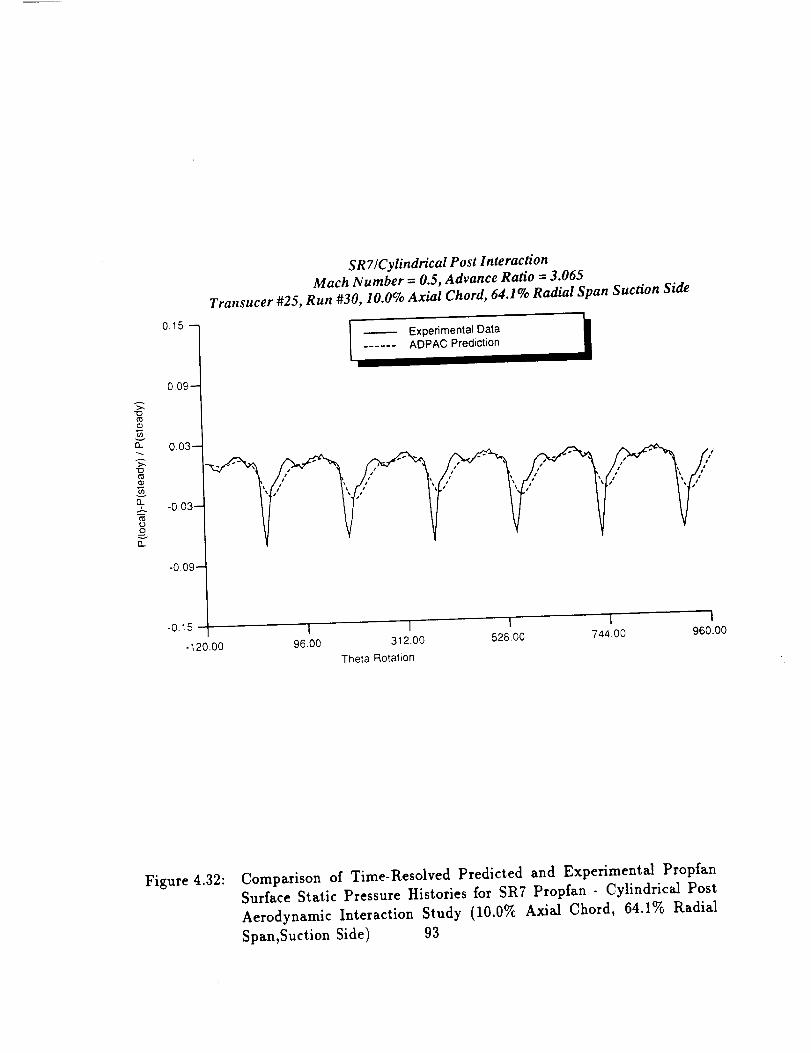
t_
t_
t_
.E
C_
ovft.
0.15 --
0.09--
0.03-
-0,03-
-0,09-
-0.15
-120.00
SR 7�Cylindrical Post Interaction
Mach Number = 0.5, Advance Ratio = 3.065
Transucer #25, Run #30, 10.0% Axial Chord, 64.1% Radial Span Suction Side
Experimental Data...... ADPAC Prediction
i
I I I I I96.00 312,00 528.00 744,00 960.00
Theta Rotation
Figure 4.32: Comparison of Time-Resolved Predicted and Experimental Propf_n
Surface Static Pressure Histories for SR7 Propfan - Cylindrical Post
Aerodynamic Interaction Study (10.0% Axial Chord, 64.1% Radial
Span,Suction Side) 93

>.,
t_
E[3..
>,"13
0_
00
0..
0.15 --
0.09--
0.03--
-0.03-
-0.09-
SR 7�Cylindrical Post InteractionMach Number = 0.5, Advance Ratio = 3.065
Transucer #23, Run #30, 36.7% Axial Chord, 64.1% Radial Span Suction Side
Experimental Data
...... ADPAC Prediction
-015 I I 1 I I-120.00 96.00 312.00 528.00 744.00 960.00
Thela Rotation
Figure 4.33: Comparison of Time-Resolved Predicted and Experimental Propfan
Surface Static Pressure Histories for SR7 Propfan - Cylindrical Post
Aerodynamic Interaction Study (36.7% Axial Chord, 64.1% Radial
Span, Suction Side) 94

0.15 --
0.09--
n 0.03--
13
-0.03-
-0.09-
SR7/Cylindrical Post Interaction
Mach Number = 0.5, Advance Ratio = 3.065
Transucer #8, Run #30, 10.0% Axial Chord, 64.1% Radial Span Pressure Side
Experimenta_ Data
...... ADPAC Prediction
-o,15 I I I I I- 120.00 96.00 312.00 528.00 744.00 960.00
Theta Rotation
Figure 4.34: Comparison of Time-Resolved Predicted and Experimental Propfan
Surface Static Pressure Histories for SR7 Propfan - Cylindrical Post
Aerodynamic Interaction Study (10.0% Axial Chord, 64.1% Radial
Span, Pressure Side) 95

>,
¢D
n
>,"13V_
[3.
O
n
0.15 --
0.09-
0.03-
-0.03-
-0.09-
SR7/Cylindrical Post InteractionMach Number = 0.5, Advance Ratio = 3.065
Transucer #10, Run #30, 36.7% Axial Chord, 64.1% Radial Span Pressure Side
Experimental Data
...... ADPAC Prediction
-0.15 I I I I I- 120,00 96.00 312.00 528,00 744.00 960.00
Theta Rotation
Figure 4.35:Comparison of Time-Resolved Predicted and Experimental Propfan
Surface Static Pressure Histories for SR7 Propfan - Cylindrical Post
Aerodynamic Interaction Study (36.7% Axial Chord, 64.1% RadialSpan, Pressure Side) 96

Figure 4.36: Predicted Instantaneous Propfan Airfoil Midspan Total Pressure Con-
tours for Cylinder/Propfan Interaction Study
97
COLOR FHO-iC,_i-:/,:'; [


also described in Section 4.2. Geometric and aerodynamic design parameters for the
model propeller are given in Figure 4.4. The calculations presented here were based
on a cruise condition with a flight Mach number of 0.72, and advance ratio of 3.14,
and forward and rearward blade setting angles of 57.4 and 60.0 degrees, respectively.
This time-dependent flow calculation is the unsteady equivalent of the steady flow
mixing plane calculations described in Section 4.2.
Time-dependent flow performance predictions for the CRP-X1 propfan were ob-
tained by using the time-dependent inter-blade row interpolation concept described
in Section 3.6. The grid therefore consists of two blocks (one for each blade row) as a
result of the simple blade count ratio (1:1). It should be noted that this grid system
corresponds to standard configuration # 7 as described in the A DPA C-A OA CR Com-
puter Program Users Manual [9]. The grid block sizes were 65x49x33 and 57x49x33,
respectively. An illustration of the mesh system is given in Figure 4.5. The time-
dependent calculation was initiated from the steady flow predictions obtained using
the mixing plane concept. In this case, because of the simple blade count ratio,
the same grid system may be used for either calculation. Once initiated, the time
dependent solution updates the data between the blade row mesh blocks based on a
time-space resolved interpolation procedure to accurately maintain the interblade row
aerodynamic interactions. The solution eventually becomes time-periodic, as shown
in the residual history given in Figure 4.37. An illustration of the time-dependent
aerodynamic interactions which occur between the counterrotating propfan airfoils is
illustrated in the instantaneous midspan static pressure contour plots given in Fig-
ure 4.38. This series of instantaneous plots illustrates the relative motion between
the propfan blade rows and the resulting static pressure field interactions which result
from this motion over one cycle of the interaction period at the blade midspan. The
interaction is obviously most intense at the point where the adjacent propfan airfoils
are lined up circumferentially. The interaction appears to have a more significant
effect on the downstream blade row, which is not unexpected since the downstream
blade row is subject to both potential and vortical disturbances while the upstream
blade row is only subject to potential disturbances.. In the absence of time-dependent
experimental data, these results can only be interpreted philosophically; however, the
overall indications are that the time-dependent flowfield has at least been captured
98


O
c_0
Model Counterrotating Propfan
-1
D2 ............................................................. f i .............................................................. _ ...............................
/ Time-Accurate Hlslor' I-- Max Residuar l
l!
m2 ............................... _............................... ' ............................... ' ............................... d...............................
_5 ................................................................................................................................................................
-60 2000 4000 6000 800010000
Iteration Number
Figure 4.37: A DPAC-A OA CR Time-Accurate Residual History for Model Counter-
Rotating Propfan Aerodynamic Interaction Analysis
99

in a reasonable manner, and has been done relatively efficiently by taking advantage
of the capabilities of the ADPA C-A OA CR code.
4.8 GMA3007 Fan Section Distortion Study (Unsteady Flow)
The final calculation to be presented is a prediction of the unsteady flow which
results from a circumferential inlet distortion in a modern turbofan engine fan sec-
tion. This calculation serves the dual purpose of analyzing a complex aerodynamic
phenomena associated with turbofan engine operation, as well as displaying the cou-
pled 2-D/3-D mesh block capabilities of the ADPAC-AOACR code. The geometry
selected for this study is the fan section of the Allison GMA3007 turbofan engine.
The Allison GMA3007 is a 5:1 bypass ratio turbofan engine which produces 7,000
pounds of thrust. The fan section geometry considered consists of three blade rows
including the fan rotor, bypass stator, and core stator. The flow is complicated by the
presence of the core flow splitter, and the fact thai there are multiple exits (bypass
flow, core flow) for which proper boundary data must be specified. An outline of the
GMA3007 fane section geometry is given in Figure 4.17.
The simulation selected involves a 6 per revolution circumferential distortion.
The distortion is represented by a stationary total pressure deficit in the incoming
flow. Each area of distortion occupies a 30 degree arc circumferentially, and is located
between 60% and 100% span radially. This particular distortion pattern was chosen
because the resulting mesh block structure can be simplified considerably compared
to other (1,2, or 3 per revolution) distortion patterns. The radial distribution of the
distortion was chosen based on experience which suggests that most fan designs are
"tip critical", suggesting that distortion effects are most critical near the fan tip. The
distortion pattern is illustrated graphically in Figure 4.39.
This calculation required a rather unique mesh block arrangement as shown in
Figure 4.40. The fan section consists of three blade rows (fan rotor, fan bypass
stator, and the core stator). The axial separation between blade rows suggest that it
is possible to solve for the rotor only in this calculation; however, previous experience
suggests that the presence of the downstream geometry, and particularly the core
flow splitter may have some influence on the time-averaged aerodynamic loading
100

1 4
!¢::
2 5
3
Figure 4.38: ADPAC-AOACR Predicted Instantaneous Static Pressure Contours at
Midspan (1 cycle of time-periodic solution)
101
COLOR DL_<:".rf ";."d;'-:I II J | _..- '*-_ _,f ,| li


Total Pressure
Distortion (6 per rev)
iiiii!ii_iiiii!iiiii
Figure 4.39: Total Pressure Deficit Pattern for Allison GMA3007 Engine Fan SectionDistortion Study
102


of the upstream rotor. Four stationary mesh blocks located upstream of the fan
rotor are utilized to impose the desired circumferential and radial distortion pattern.
The distortion is defined as a nonuniform inlet boundary condition on two of the
stationary mesh blocks, resulting in the distortion pattern previously described. The
fan rotor is represented by a mesh system discretizing four blade passages. This is the
minimum portion of the rotor which must be represented under the present distortion
pattern. The use of four blade passages permits an application of periodicity across
the rotor blade representation which is consistent with the imposed 6 per revolution
distortion pattern. It was assumed that the bypass stator and core stator did not
require more than a single blade passage representation, and therefore the bypass
stator is represented by a single 3-D blade passage mesh, and the core stator is
represented through a 2-D mesh system with embedded blade element blockage and
body forces to simulate the axisymmetric effects of the stator. This representation
was chosen to demonstrate the combined 2-D/3-D solution coupling capabilities of
the ADPAC-AOACR code. The single passage mesh blocks for the bypass stator
and the 2-D representation of the core stator are numerically coupled with the mesh
blocks for the fan rotor by using a circumferential averaging procedure. Due to time
constraints and computational limitations, a relatively sparse mesh was utilized in this
calculation, and the results should therefore be interpreted only as a demonstration
of this capability, and not conclusively representative of the truie flow.
The time-dependent calculation was initialized from a steady flow calculation
utilizing the mixing plane concept between blade rows. The time-dependent calcu-
lation was performed over approximately 4 cycles of the distortion pattern, beyond
which point a time-periodic solution was observed.
During the course of this calculation, the distortion pattern was observed to
become less well defined with axial distance from the inlet. This phenomenon was a
result of the relatively coarse mesh used in this demonstration which unrealistically
smeared the distortion pattern due to numerical dissipation. As a result, the impact
of the distortion on the rotating fan was minimized by the resulting smoothing of
the distortion as it approached the fan. This implies that for practical calculations
involving inlet distortions, a significant number of grid points must be utilized just
on the basis of distortion convection alone.
103


Figure 4.40: ADPAC-AOACR 10-Block Mesh System for Allison GMA3007 Engine
Fan Section Inlet Distortion Study
104
COLOR F;4:.,].,_'::. _ ;"


An illustration of the effects of the inlet distortion on the fan rotor are displayed
on the surface static pressure contour plot given in Figure 4.41. The effects of the
distortion are displayed clearly in the repeating pattern near the tip of the fan rotor
blades. Total pressure contours on a mesh plane downstream of the fan leading edge
at approximately 30% axial chord illustrated in Figure 4.42. This figure illustrates
the resulting total pressure distortion pattern after entering the rotor passage. Again,
the distortion continues to become less noticable with axial distance as a result of
artifical dissipation. The influence of secondary flow and aerodynamic loading on the
airfoils transform the shape of the distortion, but the overall extent of the distortion
appears to be relatively unchanged. Without experimental data to verify the results
of the analysis, no concrete conclusions can be drawn from this analysis; however, the
potential for the capability to analyze complex turbomachinery flows resulting from
inlet flow distortion has been demonstrated.
105


Figure 4.41: ADPAC-AOACR Instantaneous Predicted Rotor Surface Static Pres-sure Contours for GMA3007 Fan Operating Under Inlet Distortion
106
0,' ,_-':;X,",!. -;-,:.:L
.COLOR p'HO[OGRAPH


Figure 4.42: ADPAC-AOA CR Predicted Instantaneous Total Pressure Contours at
30% Axial Chord for the GMA3007 Fan Operating Under Inlet Distor-
tion107
,, ' :,</',,P"H


5. CONCLUSIONS
A time-dependent, three-dimensional Euler/Navier-Stokes aerodynamic analysis
has been developed for the numerical analysis of ducted and unducted fan flowfields
involving multiple blade rows. The underlying multi-block discretization scheme
provides a convenient basis upon which detailed aerodynamic analyses for compli-
cated counterrotating geometries may be performed. Multiple blade row calcula-
tions were demonstrated utilizing both the steady flow mixing plane concept and the
time-resolved interpolation procedure for rotor/stator interaction calculations. Aero-
dynamic predictions generated from the analysis were verified through comparisons
with both steady state and time-dependent experimental data. The capability of ac-
curately simulating the time-dependent aerodynamics in an advanced turbofan engine
fan section with inlet distortion has been demonstrated.
Several comments are in order concerning the various numerical techniques ap-
plied in this study. It is apparent that the algebraic turbulence model may not be
well suited for the complex vortical flows which can occur for modern turbomachinery
blade designs. Future efforts may benefit from more detailed turbulence models devel-
oped for complex 3-D flows. The time-accurate implicit residual smoothing algorithm
is also a known source of error for unsteady flow predictions. Although these errors
are suspected to be local in nature, additional studies dedicated to understanding
the impact and limitations of this algorithm may be warranted. The overall accuracy
of the analysis can be swayed by additional factors, including the unknown deflected
shape of the propfan blade, errors introduced through poor grid resolution, turbulence
modeling, and artificial dissipation. In spite of the known algorithmic deficiencies, the
analysis has successfully predicted several complex time-dependent flows with inter-
acting geometries, and has demonstrated good agreement with available experimental
data.
109
FRECEOi_i_3 P,_GE 81.ANK NO_ FILMED

110

REFERENCES
[1] Weber, K. F., and Delaney, R. A., "Viscous Analysis of Three-Dimensional
Turbomachinery Flows on Body Conforming Grids Using an Implicit Solver",
ASME Paper 91-GT-205, 1991.
[2] Chima, R. V., "Inviscid and Viscous Flows in Cascades with an Explicit
Multiple-Grid Algorithm", AIAA Journal Vol. 23, pp. 1156-1563, 1985.
[3] Wainusky, H. S., and Vaczy, C. M., "Aerodynamic Performance of a Counter
Rotating Prop-Fan", AIAA Paper 86-1550, 1986.
[4] Rai, M. M., "Unsteady Three-Dimensional Navier-Stokes Simulation of Rotor-
Stator Interactions", AIAA Paper 87-2058, 1987. 1985.
[5] Adamczyk, J. J., "Model Equations for Simulating Flows in Multistage Turbo-
machinery", ASME Paper 85-GT-226.
[6] Goyal, R. K., and Dawes, W. N.,"A Comparison of the Measured and Predicted
Flowfield in a Modern Fan-Bypass Configuration", ASME Paper 92-GT-298,1992.
[7] Hall, E. J. and Delaney, R. A., "Investigation of Advanced Counterrotation
Blade Configuration Concepts for High Speed Turboprop Systems: Task II -
Unsteady Ducted Propfan Analysis - Final Report", NASA CR 187106, NASA
Contract NAS3-25270, 1992.
[8] Crook, A. J. and Delaney, R. A., "Investigation of Advanced Counterrotation
Blade Configuration Concepts for High Speed Turboprop Systems: Task IV
- Advanced Fan Section Analysis, Final Report", NASA CR 187128, NASA
Contract NAS3-25270, 1992.
[9] Hall, E. J. and Delaney, R. A., "Investigation of Advanced Counterrotation
Blade Configuration Concepts for High Speed Turboprop Systems: Task V -
Counterrotation Ducted Propfan Analysis, Computer Program Users Manual",
NASA CR 187125, NASA Contract NAS3-25270, 1992.
111

[10] Martinelli, L., "Calculation of Viscous Flows with a Multigrid Method", Ph.D.
Dissertation, MAE Department, Princeton University, 1987.
[11] Barton, J. M., Yamamoto, O., and Bober, L. J., "Euler Analysis of Transonic
Propeller Flows," AIAA Journal, Vol. 3, June 1987, pp. 277-282.
[12] Saxer, A., "A Numerical Analysis of 3-D Inviscid Stator/Rotor Interaction Us-
ing Non-Reflecting Boundary Conditions", MIT Gas Turbine Laboratory Re-
port #209, 1992.
[13] Janus, M., Personal communication, June, 1992.
[14] Usab, W. J., Lee, A. K., and Sullivan, J. P., "A Comparison of Numerical Sim-
ulation and Experimental Measurements of Flow through Propellers," AIAA
Paper 88-0367, 1988.
[15] Saito, S., Kobayashi, H., Nakamura, Y., and Matsuo, Y., "Predicted Flow Field
Around the Advanced Propeller at Take-Off," AIAA Paper 88-3151, 1988.
[16] Matsuo, Y., Arakawa, C., Saito, S., and Kobayashi, H., "Navier-Stokes Compu-
tations for Flowfield of an Advanced Turboprop," AIAA Paper 88-3094, 1988.
[17] Kobayawa, M., and Hatano, I., "Flow Field around a Propeller by Navier-Stokes
Equation Analysis," AIAA Paper 88-3150, 1988.
[18] Celestina, M. L., Mulac, R. A., and Adamczyk, J. J., "A Numerical Simulation
of the Inviscid Flow Through a Counterrotating Propeller," ASME Paper 86-
GT-136, 1986.
[19] Whitfield, D. L., Swafford, T. W., Janus, J. M., Mulac, R. A., and Belk, D.
M., "Three-Dimensional Unsteady Euler Solutions for Propfans and Counter-
Rotating Propfans in Transonic Flow," AIAA Paper 87-1197, 1987.
[20] Hall, E. J., and Delaney, R. A., "3D Euler Analysis of Ducted Propfan Flow-
fields", AIAA Paper 90-3034-CP, 1990.
[21] Hall, E. J., Delaney, R. A., and Bettner, J. L., "Investigation of Advanced
Counterrotation Blade Configuration Concepts for High Speed Turboprop Sys-
tems: Task I - Ducted Propfan Analysis", NASA CR 185217, NASA Contract
NAS3-25270, 1990.
112

[22]
[23]
[24]
[25]
[26]
[27]
[28]
[29]
[3o]
[31]
[32t
Williams, M. H., Cho, J.,and Dalton, W. N., "Unsteady Aerodynamic Analysis
of Ducted Fans," (to appear in the AIAA Journal of Propulsion and Power).
Nallasamy, M., and Groeneweg, J. F., "Unsteady Euler Analysis of the Flow
Field of a Propfan at an Angle of Attack", AIAA Paper 90-0339, 1990.
Whipple, D., "BDX-Binary Data Exchange Preliminary Information", NASA-
Lewis Research Center, 1989.
Walatka, P. P., and Buning, P. G., "PLOT3D User's Manual,", rough draft for
NASA TM, 1988.
Plessel, Todd, "SURF User's Guide,", NASA Ames Research Center, 1988.
Walatka, P. P., and Buning, P. G., "FAST", NASA Ames Research Center,1990.
Mulac, R. A., "A Multistage Mesh Generator for Solving the Average-Passage
Equation System," NASA CR 179539, 1988.
Adamczyk, J. J., Celestina, M. L., Beach, T. A., and Barnett, M., "Simula-
tion of Three-Dimensional Viscous Flow Within a Multistage Turbine," ASME
Paper 89-GT-152, 1989.
Brackbill, J. B., and Saltzman, J. S., "Adaptive Zoning for Singular Problems
in Two Dimensions," Journal of Computational Physics, 46,342-368, 1982.
Thompson, J. F., "Elliptic Grid Generation," Numerical Grid Generation
(Edited by Joe Thompson), Elsevier Science Publishing Co., 1982.
Anderson, D. A., Tannehill, J. C., and Pletcher, R. H. , "Computational Fluid
Mechanics and Heat Transfer", McGraw-Hill, New York, New York, 1984.
[33] Hung, C. M., and Kordulla, W., "A Time-Split Finite Volume Algorithm for
Three-Dimensional Flow-Field Simulation," AIAA Paper 83-1957, 1983.
[34] Baldwin, B. S., and Lomax, H., _Thin-Layer Approximation and Algebraic
Model for Separated Turbulent FLows", AIAA Paper 78-257, 1978.
[35] Jameson, A., Schmidt, W., and Turkel, E., "Numerical Solutions of the Eu-
let Equations by Finite Volume Methods Using Runge-Kutta Time-Stepping
Schemes," AIAA Paper 81-1259, 1981.
113

[36]
[37]
[38]
[39]
[40]
[41]
[42]
Radespiel, R., Rossow, C., and Swanson, R. C., "Efficient Cell Vertex Multigrid
Scheme for the Three-Dimensional Navier-Stokes Equations", AIAA Journal,
Vol. 28, No. 8, pp. 1464-1472, 1990.
Hollanders, H., Lerat, A., and Peyret, R., "Three-Dimensional Calculation of
Transonic Viscous Flows by an Implicit Method," AIAA Journal, 23, pp. 1670-1678, 1985.
Jorgensen, P. C. E., and Chima, R. V., "An Unconditionally Stable Runge-
Kutta Method for Unsteady Flows," NASA TM 101347, 1989.
Rao, K. V., and Delaney, R. A., 1990, "Investigation of Unsteady Flow Through
a Transonic Turbine Stage: Part I- Analysis", AIAA Paper 90-2408.
Bushnell, P., "Measurement of the Steady Surface Pressure on a Single Rotation
Large Scale Advanced Prop-Fan Blade at Mach Numbers from 0.03 to 0.78,"NASA CR 182124, 1988.
Bushnell, P., Gruber, M., and Parzych, D., "Measurement of Unsteady Blade
Surface Pressure on a Single Rotation Large Scale Advanced Prop-Fan with
Angular and Wake Inflow at Math Numbers from 0.02 to 0.70", NASA CR-
182123, NASA Contract NAS3-23051, 1988.
Steffen, F. W., "Cruise Performance of an Isolated 1.15 Pressure Ratio Turbofan
Propulsion Simulator at Mach Numbers from 0.6 to 0.85," NASA TM X-3064,1974.
[43] Wesoky, H. L., Abbott, J. M., Albers, J. A., and Dietrich, D. A., "Low-Speed
Wind Tunnel Tests of a 50.8 Centimeter (20-in.) 1.15 Pressure Ratio Fan Engine
Model," NASA TM X-3062, 1974.
[44] Smith, S. M., "Discrete Frequency Sound Generation in Axial Flow Turboma-
chines", University of Cambridge, Department of Engineering Report CUED/A-Turbo/TR 29, 1971.
[45] Huff, D. L., "Pressure Wave Propagation Studies for for Oscillating Cascades",
AIAA Paper 92-0145, 1992.
[46] Wesoky, F. L., and Steffen, F. W., "Wind Tunnel Tests of a 20 in. Diameter
1.15 Pressure Ratio Fan Engine Model," NASA TM X-71445, 1973.
114

[47] Osborn, W. M., and Steinke, R. J., "Performance of a 1.15 Pressure-Ratio
Axial-Flow Fan Stage with a Blade Tip Solidity of 0.5," NASA TM X-3052,
1974.
115

116

APPENDIX A. ADPAC DISTRIBUTION LIST
ADPAC DISTRIBUTION LIST
NASA Contract NAS3-25270
Task Order #2
User's Manual CR-187125
Final Report CR-187126
GOVERNMENT AGENCIES:
NASA Headquarters
600 Independence Avenue, SW
Washington, DC 20546
Attn: RJ/C. C. Rosen
RP/S. Wander
RP/J. R. Facey
NASA Lewis Research Center
21000 Brookpark Road
Cleveland, OH 44135
Attn: J.J. Adamczyk
C. L. Ball
L. J. Bober
D. R. Boldman
B. Clark
R. W. Claus
J. H. Dittmar
J. F. Groeneweg
C. E. HughesR. J. Jeracki
C. M. Kim
J. Lytle
M.S. 5-9 (2 copies)
M.S. 86-1
M.S. 77-6
M.S. 86-7
M.S. 77-6
M.S. 142-5
M.S. 77-6
M.S. 77-6 (2 copies)
M.S. 77-6
M.S. 77-6
M.S. 77-6
M.S. AAC-1
117

A. J. Mahajan M.S. 23-3
C. J. Miller M.S. 77-6
D. P. Miller M.S. 77-6
R. D. Moore M.S. 77-6
L. D. Nichols M.S. 142-5
C. W. Putt M.S. 142-2
D. R. Reddy M.S. 5-11
T. S. Reddy M.S. 23-3
R. Srivastava M.S. 23-3
G. L. Stefko M.S. 23-3
R. P. Woodward M.S. 77-6
J. A. Ziemianski M.S. 86-1
Report Control Office M.S. 60-1
Tech. Utilization Office M.S. 7-3
AFSC Liaison Office M.S. 501-3
NASA Ames Research Center
Moffett Field, CA 94035
Attn: Library M.S. 202-3
NASA Langley Research Center
Hampton, VA 23665
Attn: F. Farassat M.S. 461
M. H. Dunn M.S. 904
Library M.S. 185
NASA Scientific and Technical Information FacilityP.O. Box 8757
BWI Airport, MD 21240
Attn: Accession Dept. (6 copies and the FF427 form)
Sverdrup Technology, Inc.
2001 Aerospace Parkway
Brookpark, OH 44142
Attn: J. Bridges M.S. 77-6
E. Envia SVR-3
R. M. Nallasamy SVR-3
S. M. Ramachandra SVR-3
O. Yamamoto SVR-3
(15 copies)
(2 copies)
(4 copies)
118

ENGINE MANUFACTURERS
Allison Gas Turbine Division, GMC Corp.
P.O. Box 420
Indianapolis, IN 46206-0420
Attn: P.l_ilI_trpaff- 144
R. F. Alverson
D. W. Burns
R. A. Delaney
J. R. Rathman
D. J. Helton
A. J. Crook
K. P. Nardini
General Electric Company
Aircraft Engine Group
1 Neumann Way
Evendale, OH 45215
Attn: P. Gliebe
C. Lenhardt
M. Majjigi
M. Pearson
L. Smith
C. Whitfield
Hamilton Standard Division - UTC
Windsor Locks, CT 06096
Attn: D. B. Hanson
F. B. Metzger
Pratt & Whitney Aircraft - UTC
Commercial Products Division
400 Main Street
East Hartford, CT 06108
Attn: D. Hopwood
D. Mathews
W. Lord
T. Wynosky
Mail Stop T-14A
Mail Stop T-14A
Mail Stop T-14A
Mail Stop T-14A
Mail Stop T-14A
Mail Stop T-14A
Mail Stop T-14A
Mail Drop A-304
Mail Drop A-330
Mail Drop A-319
Mail Drop A-317
Mail Drop H-4
Mail Drop A-304
M.S. 1A-3-6
M.S. 1A-3-6
M.S. 162-07
M.S. 165-11
M.S. 169-23
M.S. 169-23
(3 copies)
119

United Technologies Corporation Research Center
Silver Lane
E. Hartford, CT 06108
Attn: M. Barnett
R. Davis
D. Dorney
M.S. 20
M.S. 20
M.S. 20
AIRFRAME MANUFACTURERS
Boeing Commercial Airplane Company (BCAC)
P.O. Box 3707
Seattle, WA 98124-2207
Attn: B. W. Farquhar
W-H. Jou
R. Cuthbertson
M.S. 0L-22
M.S. 7H-96
M.S. 79-84
Douglas Aircraft Company Division
McDonnell Douglas Corporation
3855 Lakewood Blvd.
Long Beach, CA 90846
Attn: M. Joshi
F. Lynch
G. Page
W. Siegele
M.S. 36-60
M.S. 36-60
M.S. 35-86
M.S. 202-15
General Dynamics Convair
P.O. Box 80844
San Diego, CA 92138
Attn: B. BergmanS. Strande
K. Taylor
M.Z. 36-1240
M.Z. 55-6950
M.Z. 54-6890
UNIVERSITIES
Georgia Institute of Technology
School of Aerospace Engineering
Atlanta, GA 30332-0800
Attn: Dr. L. N. Sankar
120

Lockheed-California Company
P.O. Box 551
Burbank, CA 91520
Attn: Library
Ohio State University
Department of Aeronautical
and Astronautical Engineering
Columbus, OH 43220
Attn: Prof. G. M. Gregorek
Pennsylvania State University
Department of Aerospace Engineering
233 Hammond Building
University Park, PA 16802
Attn: Dr. B. Lakshminarayana
Purdue UniversitySchool of Aeronautics and Astronautics
W. Lafayette, IN 47907
Attn: Dr. J. P. Sullivan
Dr. M. Williams
Purdue University
School of Mechanical Engineering
W. Lafayette, IN 47907
Attn: Dr. S. Fleeter
Rohr Industries, Inc.
P.O. Box 878
Chula Vista, CA 92012-0878
Attn: Library
Texas A&M University
Aerospace Engineering Department
College Station_ TX 77843-3141
121

Attn: Dr. K. D. Korkan
University of ArizonaAerospace and Mechanical Engineering Department
Aero Building #16
Tucson, AZ 85721
Attn: Dr. E. J. Kerschen
University of Missouri-Rolla
Mechanical Engineering Department
Rolla, MO 65401-0249
Attn: Dr. Walter Eversman
Mississippi State University
Department of Aerospace Engineering
P.O. Box A
Mississippi State, MS 39762
Attn: Dr. D. Whitfield
Dr. M. Janus
122

NA %t_al_ Aeronaulcs and,5_oace A_,"_s_ta_,o,_
1. Report No,
NASA _ 187126
4. Title a'nd Subtitle
Report Documentation Page
2. Government Accession No. 3. Recipient's Catalog No.
Investigation of Advanced Counterrotating Blade Config-
uration Ooncepts for High SPeed Turboprop Systems,
Task 5 - Unsteady Counterrotation Ducted Propfan
Analysis, Final Report
7. Authorls)
Edward J. Hall and _obert A. Delaney
9. Performing Organization Name and Address
Allison Gas Turbine Division General Motors Corporation
P.O. Box 420, Speed Code TI4A
Indianapolis, IN 46206-0420
5. Report Date
January 1993
'6. Performing Organization Code
8. Performing Organization Report No.
10. Work Unit No.
535-03-10
11. Contract or Grant No.
NAS3-25270
13. Type of Report and Period Covered
Contract Report, Final
14. Sponsoring Agency Code
12. Sponsoring Agency Name and Address
National Aeronautics and Space Administration
Lewis Research Center
21000 Brookpark Road
Cleveland, OH 44135-3191
15. Supplementary Notes
Prepared in oooperation with NASA _roject _nnager, Christopher J. Miller,
NASA Lewis Research Center, Cleveland, OH
16. Abstract The primary objective of this study was the development of a time-marching
three-dimensi6nal Euler/Navier-Stokes aerodynamic analysis to predict steady and
unsteady compressible transonic flows about ducted and unducted propfan propuslion
systems (mloloying multiple blade rows. The computer codes resulting from this
study are referred to as ADPAC-AOACR (Advanced Ducted Propfan Analysis Codes-
Angle of Attack Coupled Row).
This document is the Final Report describing the theoretical basis and analytical
results from the ADPAC-AOACR codes developed under Task 5 of NASA Contract
NAS3-25270, Unsteady Counterrotating Ducted Propfan Analysis.
The ADPAC-AOACR program is based on a flexible multiple blocked grid
discretization scheme permitting coupled 2-D/3-D mesh block solutions with appli-
cation to a wide variety of geometries. For convenience, several standard mesh
block structures are described for turbomachinery applications. Aerodynamic
calculations are based on a four-stage Runge-Kutta time-marching finite volt, he
solution technique with added numerical dissipation. Steady flow predictions are
accelerated by a nmltigrid procedure. Numerical calculations are compared with
experimental data for several test cases to demonstrate the utility of this approach
l_Qrey WordJ(Suggested by Authorls)) ' i " tatement _ltiDle blade rows.-
Navier-Stokes Turbomachinery :
Fan _hltiple Block i Unclassified-UnlimitedDucted ADPAC ;
19. Security C)ass,f. (of this report)L
Unclassified
NASA FORM 1626 OCT 86
20. Security Classif (of this page)
Unclassified
21 No of pages 22 Price
A06