INVESTIGATION OF SEDIMENT EROSION RATES OF ROCK ... - University of Floridaufdcimages.uflib.ufl.edu/UF/E0/04/24/76/00001/crowley_r.pdf · mixtures for predicting scour depth using

INVESTIGATION OF SEDIMENT EROSION RATES OF ROCK, SAND, AND CLAY MIXTURES FOR PREDICTING SCOUR DEPTH USING ENHANCED EROSION RATE

TESTING INSTRUMENTS

By

RAPHAEL CROWLEY

A DISSERTATION PRESENTED TO THE GRADUATE SCHOOL OF THE UNIVERSITY OF FLORIDA IN PARTIAL FULFILLMENT

OF THE REQUIREMENTS FOR THE DEGREE OF DOCTOR OF PHILOSOPHY

UNIVERSITY OF FLORIDA

2010

2

© 2010 Raphael Crowley

3

To my sister, Mary

4

ACKNOWLEDGMENTS

First and foremost, I thank my family for their continued support through the years. My

mom’s always been there for me, and she was always someone I could turn to when I needed

something. My dad’s wisdom and guidance through graduate school – from coursework, to

switching advisors twice, through qualifying exams, and through the dissertation process – made

it possible for me to complete what I needed to. His perspective as a professor at a 4-year

institution gave me the insight I always needed to figure out what I was supposed to do. Finally,

my sister, Mary, for whom this dissertation is dedicated has always been the best little sister on

the planet. She’s always willing to listen to me talk about anything – school related or otherwise

– and she’s become one of my best friends through my life. Thanks Mar! You Rock!

Secondly, I thank the University of Florida Women’s Rowing Team for their support

throughout graduate school, and for giving me the opportunity to coach during my time here at

UF. Particularly, I thank the UF Crew Novice class of 2010; those women have taught me so

much, and have helped keep me sane through the years. Special shout-outs from that class go to

(in no particular order) Liz Commins, Courtney Holst, Emily Congdon, Katie Tschopp, Haley

Kress, Anna Kantzios, and Laura Thomas. You kids have taught me so much, meant the world

to me, and I couldn’t have finished grad school without you guys and everyone else from the

Women’s Team. My only regret has been to cut out on you during your senior year so that I

could get this Ph.D. done. Thanks also to Justin Knust for making Florida Crew what it was

supposed to be, coaching me for a year, talking me into coaching, and for being a mentor and a

friend for me through the years.

Third, thanks to anyone who helped me in the lab or administratively during my time

working on my Ph.D. Falak Shah, Courtney Holst, Jim Hayne, Randall Booker, and Arden

Herrin have been great undergrad assistants, and I have loved working with them. Chuck

5

Broward, James “JJ” Joiner, and Hubert “Nard” Martin, Danny Brown, and Vic Adams have

been the best support staff I ever could have hoped for. Thanks also to Debra Hambrick, Lucy

Hamm, Carolyn Carpenter, Donna Moss, Nancy McIlrath, and Tony Murphy for dealing with the

money, computers, paperwork, and everything else administrative that needed to be done.

Fourth, thanks to my friends who supported me during the “Raf Crowley 2010 plan” or the

plan for me to spend a solid decade doing college things. It was a big joke in undergrad

(modeled after Bucknell’s 2010 plan), but it seriously happened, and I can’t thank you guys

enough for putting up with me through it all. Special thanks to the McCullough family – Mr. and

Mrs. Tracy McCullough, Aaron and Kim McCullough, and Mikey and Michelle McCullough –

for always having my back and being like a 2nd family to me. Thanks to my undergrad group of

friends, Chuck Dickhart, Matt Albrecht, Beau Bryant, Kyle McNeel, Leo Nalini, Bryan Prins,

Tom Leary (R.I.P.), Adam Linetty, and the guys at Lambda. Thanks to my teammates and

friends in grad school– you taught me what a true team was supposed to be. Particularly thank

you Timmy Lucas, Jon Levy, Brian Suggs, Adam Kallin, Bill Griffith, Andrew Wellbourne, Ben

Michael, Trevor Guynes, Geoff Scharfenburger, Danny Reach, Ben Bolz, Shane Laakso, Andy

Selepak, Jen Haas, Neil W. Blackmon, and Derek Snyder. Finally, thanks to my friends that

have been with me for forever – Brandon Phinney, Matt Johnston, Price Taggert, Chris Cooper,

and Chris Wickman.

Fifth, I must thank a few professors in particular who helped to make this Ph.D. possible.

Dr. Richard Crago from Bucknell University gave me my start in research and I definitely would

not be here today if it wasn’t for working with him for two summers while in undergrad. Thanks

to my committee members, Dr. David Prevatt and Dr. Toshi Nishida. My co-chair, Dr. D. Max

Sheppard was a great advisor for my Masters degree, and he was a valuable committee member

6

during this dissertation. I thank him for giving me the opportunity to go to the TFHRC and work

with Kornel Kerenyi – that background helped to make my work with the SERF possible.

Kornel and Dr. Sheppard were wonderful mentors to me over the years. Finally, thank you so

much Dr. Bloomquist for giving me the chance to work with you on this project. You have been

the best advisor I ever could have hoped for, and I cannot imagine completing a dissertation with

anyone else. You were endlessly patient with me, you were always encouraging, and you were

always able to help me when I needed it. To Dr. Bloomquist, my professors, my team, my

family, my friends, and everyone else – thank you all so much!

7

TABLE OF CONTENTS page

ACKNOWLEDGMENTS ...............................................................................................................4

LIST OF TABLES .........................................................................................................................13

LIST OF FIGURES .......................................................................................................................14

ABSTRACT ...................................................................................................................................26

CHAPTER

1 INTRODUCTION ..................................................................................................................28

1.1 Motivation for Research ..............................................................................................28 1.2 Scour Definitions .........................................................................................................29

1.2.1 General Scour.....................................................................................................30 1.2.2 Aggradation/Degradation ...................................................................................30 1.2.3 Contraction Scour ..............................................................................................30 1.2.4 Local Scour ........................................................................................................31

1.3 Controversy Surrounding HEC-18 ..............................................................................32 1.4 Approach ......................................................................................................................33 1.5 Methodology and Organization ...................................................................................35

2 BACKGROUND AND LITERATURE REVIEW ................................................................39

2.1 Scour Depths in Non-Cohesive Soil .................................................................................39 2.2 Predicting Local Scour Hole Depth for Cohesive Soils and Rock ...................................39

2.2.1 Colorado State University Tests (CSU 1991 - 1996) .............................................40 2.2.1.1 Setup for CSU tests ......................................................................................41 2.2.1.2 Results from CSU tests ................................................................................41 2.2.1.3 Concerns with the CSU correction factor.....................................................42

2.2.2 The EFA-SRICOS Method .....................................................................................42 2.2.2.1 HEC-18 version of EFA-SRICOS method ...................................................43 2.2.2.2 Complete version of EFA-SRICOS method ................................................43 2.2.2.3 EFA-SRICOS setup discussion ....................................................................44 2.2.2.4 Discussion of Equation 2-3 ..........................................................................44

2.2.3 The Miller-Sheppard Method .................................................................................47 2.2.4 Scour Depth for More Complex Structures ............................................................51

2.3 Analytical Methods for Determining Erosion Rate-Shear Stress Relationships ..............53 2.3.1 Particle-Like vs. Rock-Like Erosion and Shields (1936) .......................................53

2.3.1.1 Einstein (1943) and Christensen (1975) .......................................................55 2.3.1.2 Wiberg and Smith (1987) .............................................................................56 2.3.1.3 Dade and Nowell (1991) ..............................................................................57 2.3.1.4 Dade et al. (1992) .........................................................................................58 2.3.1.5 Mehta and Lee (1994) ..................................................................................58

8

2.3.1.6 Torfs et al. (2000) .........................................................................................59 2.3.1.7 Sharif (2002) ................................................................................................60 2.3.1.8 Critical shear stress discussion .....................................................................61 2.3.1.9 Partheniades (1962) ......................................................................................61 2.1.1.10 Christensen (1975) .....................................................................................62 2.3.1.11 McLean (1985) ...........................................................................................62 2.3.1.12 Van Prooijen and Winterwerp (2008) ........................................................63

2.3.2 Analytical Methods for Determining Rock Erosion ...............................................64 2.3.2.1 Cornett et al. (1994) and Henderson (1999) .................................................65 2.3.2.2 Stream power method ...................................................................................66

2.4 Empirical Methods for Measuring Scour and Erosion in Cohesive Soils and Rock ........67 2.4.1 Erosion Rate-Shear Stress Standards for Rock ......................................................68

2.4.1.1 Geologic, geomorphologic, and geotechnical analyses (Richardson and Davis 2001) ...........................................................................................................68

2.4.1.2 July 1991 FHWA “Scourability of Rock Formations” (Gordon 1991)........68 2.4.1.3 Erodibility index method (Annandale et al. 1996) .......................................71 2.4.1.4 Flume tests (Richardson and Davis 1991) ....................................................72

2.4.2 Erosion Rate Testing Devices ................................................................................72 2.4.2.1 Nalluri and Alvarez (1992)...........................................................................72 2.4.2.2 Mitchener and Torfs (1996) .........................................................................73 2.4.2.3 Panagiotopolous et al. (1997) .......................................................................73 2.4.2.4 SEDFlume (McNeil et al. 1996, Jepsen et al. 1997) ....................................74 2.4.2.5 ASSET (Roberts et al. 2003) ........................................................................77 2.4.2.6 EFA (Briaud et al. 1991-2004) .....................................................................78 2.4.2.7 RETA (Henderson 1999 Kerr 2001 and Slagle 2006) .................................80 2.4.2.8 Barry et al. (2003) ........................................................................................85 2.4.2.9 SERF (Trammel 2004, Slagle 2006, Kerr 2001) ..........................................85

2.5 Gator Rock ........................................................................................................................89 2.5.1 Gator Rock: A Brief History and Description ........................................................89 2.5.2 Extension of Gator Rock to Flume Tests ...............................................................90 2.5.3 Gator Rock 2.0 ........................................................................................................91 2.5.4 Gator Rock 3.0 ........................................................................................................92 2.5.5 Need for Better Gator Rock ....................................................................................93

3 ENHANCEMENTS AND IMPROVMENTS TO THE SEDIMENT EROSION RATE FLUME .................................................................................................................................117

3.1 Introduction .....................................................................................................................117 3.2 Laser Leveling System ...................................................................................................117 3.3 Temperature Control System and Temperature Patch for SEATEK ..............................123 3.4 New Shear Stress System ...............................................................................................126

3.4.1 Shear Stress Sensor ...............................................................................................126 3.3.2 New Pressure Transducers ...................................................................................129 3.4.3 Paddlewheel Flow meter ......................................................................................130

3.5 Sediment Control System ...............................................................................................131 3.5.1 Filter System .........................................................................................................131 3.5.2 Sand Injector .........................................................................................................135

9

3.6 Vortex System ................................................................................................................136 3.7 Miscellaneous Other Enhancements to the SERF ..........................................................138 3.8 Summary of SERF Improvements and Brief Discussion ...............................................140

4 ESTIMATIONS AND MEASUREMENTS OF SHEAR STRESSES ON AN ERODING BED MATERIAL IN FLUME-STYLE EROSION RATE TESTING DEVICES .............................................................................................................................151

4.1 Executive Summary ........................................................................................................151 4.2 Review of Relevant Background ....................................................................................151 4.3 Experimental Setup .........................................................................................................153 4.4 Experimental Results and Discussion .............................................................................155

4.4.1 Pressure Drop .......................................................................................................155 4.4.2 Analytical Methods ..............................................................................................160 4.4.3 Vortex Conditions ................................................................................................161

4.5 Recommendations and Conclusions ...............................................................................162 4.6 Future Work ....................................................................................................................163

5 DEVELOPMENT AND TESTING WITH A NEARLY UNIFORM, HIGHLY ERODIBLE, SYNTHETIC ROCK-LIKE MATERIAL TO BE USED FOR CALIBRATING EROSION-RATE TESTING DEVICES..................................................178

5.1 Executive Summary ........................................................................................................178 5.2 Review of Relevant Background ....................................................................................178 5.3 Theory Behind Bull Gator Rock .....................................................................................181 5.4 Procedure for Construction of “Bull Gator Rock” .........................................................182 5.5 First Gator Rock Mix ......................................................................................................184

5.5.1 Mix Compositions ................................................................................................184 5.5.2 Strength Tests .......................................................................................................184 5.5.3 RETA Tests ..........................................................................................................185

5.5.3.1 First round of tests on first batch of Gator Rock in RETA ........................185 5.5.3.2 Second round of tests on first batch of Gator Rock in RETA ....................187

5.5.4 SERF Tests ...........................................................................................................191 5.5.4.1 Shear stress tests .........................................................................................191 5.5.4.2 Erosion tests ...............................................................................................192 5.5.4.3 SERF analysis ............................................................................................197

5.6 Second Gator Rock Mix .................................................................................................198 5.6.1 Tensile and Compressive Strength Tests ..............................................................200 5.6.2 RETA Tests ..........................................................................................................201 5.6.3 Absorption Limits .................................................................................................202

5.7 Discussion .......................................................................................................................203 5.8 Summary and Conclusions .............................................................................................205 5.9 Future Work ....................................................................................................................206

10

6 VERIFICATION OF THE ROTATING EROSION TESTING APPARATUS (RETA) AND USING RETA RESULTS TO PREDICT EROSION RATES AND SHEAR STRESSES OF ERODING BED MATERIALS USING COHESION ...............................223

6.1 Executive Summary ........................................................................................................223 6.2 Review of Relevant Background ....................................................................................223 6.3 RETA Verification ..........................................................................................................226 6.4 Extending RETA Results – Predicting Erosion Rate as a Function of Material

Strength .............................................................................................................................228 6.4.1 Approximation of M .............................................................................................228 6.4.2 Dimensional Analysis ...........................................................................................229 6.4.3 Approximating τc ..................................................................................................230

6.5 Discussion and Future Work ..........................................................................................232 6.6 Summary and Conclusions .............................................................................................234

7 A STUDY OF EROSION RATES, SHEAR STRESSES AND DENSITY VARIATIONS OF SAND/CLAY MIXTURES ..................................................................242

7.1 Executive Summary ........................................................................................................242 7.2 Review of Relevant Background and Motivation for Research .....................................242 7.3 Materials and Procedure .................................................................................................243

7.3.1 Materials ...............................................................................................................244 7.3.2 Shear Stresses .......................................................................................................244 7.3.3 Mixing Procedure .................................................................................................246

7.3.3.1 Sand mixing procedure ...............................................................................247 7.3.3.2 Sand-clay mixing procedure .......................................................................247

7.3.4 SERF Testing ........................................................................................................248 7.3.5 Procedural Variations ...........................................................................................249 7.4.6 Density Profile Tests ............................................................................................250

7.4 Experimental Results and Analysis ................................................................................250 7.4.1 Shear Stress Tests .................................................................................................250 7.4.2 SERF Tests ...........................................................................................................252

7.4.2.1 Zero-percent clay mixture ..........................................................................252 7.4.2.2 Twenty-five percent clay samples ..............................................................255 7.4.2.3 Fifty-percent clay samples .........................................................................261 7.4.2.4 Seventy-five percent clay mixture ..............................................................264 7.4.2.5 One-hundred percent clay ..........................................................................265

7.4.3 Density Profile Tests ............................................................................................265 7.4.4 Effects of Sand Concentration on Shear Stresses .................................................268

7.5 Summary and Conclusions .............................................................................................270 7.6 Future and Ongoing Work ..............................................................................................271

8 SUMMARY AND FUTURE WORK ..................................................................................302

8.1 Summary .........................................................................................................................302 8.1.1 Review of Goals for This Study ...........................................................................302 8.1.2 Summary of Work ................................................................................................302

11

8.2 Conclusions.....................................................................................................................303 8.3 Future Work ....................................................................................................................304

8.3.1 Essential Final Improvements to the SERF ..........................................................304 8.3.2 Non-Essential Final Improvements to the SERF ..................................................306 8.3.3 Determine Erosion Patterns for Natural Sand-Clay Mixtures ..............................308 8.3.4 Roughness Number Tests or Improved Testing Apparatus ..................................308 8.3.5 Normal Stress Measurements in SERF ................................................................309 8.3.6 Normal Stress Measurements under Field Conditions .........................................309 8.3.7 Computer Model ...................................................................................................310 8.3.8 Summary of Proposed Future Progression ...........................................................310

APPENDIX

A SCOUR DEPTHS IN NON-COHESIVE SOILS .................................................................311

A.1 Introduction ....................................................................................................................311 A.2 HEC-18: Basic Principles (Richardson and Davis 2001) ..............................................312

A.2.1 HEC-18: Long Term Aggradation and Degradation (Richardson and Davis 2001) ..........................................................................................................................312

A.2.2 HEC-18: Contraction Scour (Richardson and Davis 2001) .................................313 A.2.3 HEC-18: Local Scour (Richardson 2001) ..........................................................314 A.2.4 HEC-18: Brief Discussion ...................................................................................318

A.3 The Florida DOT Bridge Scour Manual ........................................................................318 A.3.1 Local Scour: Motivation for a Different Computation Algorithm ......................318 A.3.2 FDOTBSM: Local Scour Equations (Florida DOT Bridge Scour Manual

2005) ..........................................................................................................................321 2.2.2.4 FDOTBSM: brief discussion ......................................................................325

B FLORIDA METHOD FOR SERF TESTS ...........................................................................334

B.1 New Operating Procedure for SERF ..............................................................................334 B.2 Preliminary Procedure for Tests ....................................................................................334

B.2.1 Vortex Generator .................................................................................................335 B.2.2 Temperature Control and Filtering ......................................................................335

B.3 Stand-Alone Shear Stress Test .......................................................................................336 B.4 Critical Shear Stress Test in SERF ................................................................................340 B.5 Erosion Rate Test ...........................................................................................................342 B.6 Remote SERF Operation ................................................................................................345

B.6.1 Remote Visual Inspection ....................................................................................346 B.6.2 Remote Labview Operation .................................................................................346

B.7 SERF Operation Troubleshooting ..................................................................................347

C SERF COMPUTER CONTROL PROGRAMS ...................................................................365

C.1 Introduction ....................................................................................................................365 C.2 Pump Control .................................................................................................................368

C.2.1 Block Diagram Explanation .................................................................................369

12

C.2.2 Front Panel Operation ..........................................................................................371 C.3 Motor Mover ..................................................................................................................371

C.3.1 Block Diagram Discussion ..................................................................................371 C.3.2 Front Panel Discussion ........................................................................................372

C.4 SERF Control No Motor ................................................................................................372 C.4.1 Block Diagram Discussion ..................................................................................373

C.4.1.1 SC-2345 channels ......................................................................................373 C.4.1.2 Pump input .................................................................................................374 C.4.1.3 Analog output ............................................................................................374

C.4.2 Front Panel Operation ..........................................................................................375 C.5 SERF Control Full (Temperature Patch) .......................................................................375

C.5.1 SERF Control Full Block Diagram Discussion ...................................................376 C.5.1.1 Pre-input sequence .....................................................................................376 C.5.1.2 Pump input .................................................................................................377 C.5.1.3 Analog output ............................................................................................377 C.5.1.4 Laser input .................................................................................................378 C.5.1.5 SEATEK output .........................................................................................378 C.5.1.6 Motor advancement ...................................................................................382 C.5.1.7 Data writing ...............................................................................................383

C.5.2 Using the Front Panel ..........................................................................................383

LIST OF REFERENCES .............................................................................................................405

BIOGRAPHICAL SKETCH .......................................................................................................413

13

LIST OF TABLES

Table page 5-1 Niraula’s Original Gator Rock Water-Cement Ratios .....................................................207

5-2 Water, Cement, and Limestone Composition for First Round Bull Gator Rock Mix .....207

5-3 Water, Cement, and Limestone Composition for Second Round Gator Rock Mix .........207

5-4 Strength Test Results from Round 2 of Gator Rock Testing ...........................................208

5-5 Actual W/C Ratios for Second Round of Gator Rock .....................................................209

7-1. Density Profile Results ....................................................................................................274

A-1 Values for k1 .....................................................................................................................326

A-2 Pier Nose Shape Correction Factors ................................................................................326

A-3 Bed Condition Correction Factors ...................................................................................327

14

LIST OF FIGURES

Figure page 1-1 Photograph of the Schoharie Creek Bridge Collapse ........................................................37

1-2 Beginning of local scour ....................................................................................................37

1-3 Local scour after some time has elapsed (Slagle 2006) .....................................................38

2-1 Results from CSU Pier Scour Study ..................................................................................94

2-2 Comparison Between Hjorth’s Results (Top) and Briaud’s Computer Model (Bottom). ............................................................................................................................94

2-3 3-D Idealized Scour Hole ...................................................................................................95

2-4 Definition Sketch from 3-D Ideal Scour Hole ...................................................................95

2-5 Second Definition Sketch from 3-D Ideal Scour Hole ......................................................96

2-6 Top-View of Pile Definition Sketch ..................................................................................96

2-7 Effective Shear Stress vs. Scour Hole Depth .....................................................................97

2-8 Extended Shields Diagram .................................................................................................97

2-9 Ariathurai-Partheniades Relationship for Erosion vs. Shear Stress ...................................98

2-10. Results from Modification of Partheniades Equation ........................................................98

2-11 Definition Sketch for Rock Fracture ..................................................................................99

2-12 ERI Definition Sketch ........................................................................................................99

2-13 Relationship between bulk density and critical shear stress ............................................100

2-14 Erosion Rate vs. Excess Shear Stress Relationships ........................................................100

2-15 Critical Shear Stress vs. % Fines Relationships...............................................................101

2-16 Original Schematic Diagram of SEDFlume ....................................................................101

2-17 Flow Rate vs. Shear Stress Relationship..........................................................................102

2-18 Example of SEDFlume Results .......................................................................................102

2-19 Original Schematic of the ASSET ...................................................................................103

15

2-20 Results from ASSET Tests ..............................................................................................103

2-21 Photograph of the EFA ....................................................................................................104

2-22 Schematic of 1 mm EFA protrusion into flume ...............................................................104

2-23 An example of a Moody Diagram ...................................................................................105

2-24. Photograph of the RETA .................................................................................................105

2-25 RETA Sample Annulus....................................................................................................106

2-26 RETA Sample Annulus (Close-up) .................................................................................106

2-27 Schematic Diagram of RETA ..........................................................................................107

2-28 Photograph of Torque Cell in RETA ...............................................................................107

2-29 Photograph of Rock Sample in RETA .............................................................................108

2-30 Top View of RETA ..........................................................................................................108

2-31 Relationship between shear stress and erosion rate for different Jewfish Creek Limestone samples ...........................................................................................................109

2-32 Relationship between cohesion and erosion rate for different shear stresses from Jewfish Creek Limesonte data set ....................................................................................109

2-33 Definition sketch for Cohesion Derivation ......................................................................110

2-34 Typical results from Slagle’s Gator Rock tests. The pink data points are from the SERF and the blue data points are from the RETA .........................................................110

2-35 Photograph of the SERF (Side View) ..............................................................................111

2-36 Top View of the SERF (Original Design) .......................................................................111

2-37 Pumps used to drive water through the SERF .................................................................112

2-38 Eroding Sample Section of the SERF ..............................................................................112

2-39 Viewing Window on SERF .............................................................................................113

2-40 Schematic Drawing of Ultrasonic Ranging System.........................................................113

2-41 Top View of Ultrasonic Depth Sensor on SERF .............................................................114

2-43 Comparison Between Rokni’s Experimental and Numerical Results .............................115

16

2-44 Trammel’s Results for Cohesive Material from Jackson County, FL .............................115

2-45 Graph of Typical Temperature Rise During Longer SERF Tests ....................................116

2-46 Eroded Gator Rock 2.0 Sample .......................................................................................116

3-1 Photograph of Laser Leveling System (the third laser is blocked by the camera angle) .141

3-2 Photograph of Amplifiers and Control Boxes for the Laser Leveling System ................141

3-3 Water Chiller ....................................................................................................................142

3-4 Temperature Drop after Water Chiller Installation ..........................................................142

3-5 Inner Components of the Shear Stress Sensor .................................................................143

3-6 Shear Stress Sensor Amplifier .........................................................................................144

3-7 Modified A/C Unit for Shear Stress Sensor Temperature Control ..................................144

3-8 Shear Stress Sensor Box with Tube From A/C Unit .......................................................145

3-9 New Pressure Transducers in SERF ................................................................................145

3-10 Trammel’s Original Flow Rate vs. Pump Frequency ......................................................146

3-11 New Pump Frequency vs. Velocity Curve .......................................................................146

3-12 Sand Injector Load Cell Mounts ......................................................................................147

3-13 Sand Injector Expansion Joints ........................................................................................147

3-14 Completed Sand Injector..................................................................................................148

3-15 Gap Ratio Effects on Vortex Development .....................................................................149

3-16 Graph of Strouhal Number vs. Reynolds Number ...........................................................149

3-17 Vortex Generator installed in SERF (looking into flume) ...............................................150

4-1 Spectral analysis of de-meaned pressure transducer voltages .........................................165

4-2 Spectral analysis of de-meaned shears stress sensor measurements ................................165

4-3 The 30 Hz data block from the shear stress sensor showing shear stress difference from the mean ..................................................................................................................166

4-4 4 Hz – 20 Hz data block from pressure transducer showing voltage difference from the mean ...........................................................................................................................166

17

4-5 Spectral analysis of free-vibratory flume test voltage measurements .............................167

4-6 Spectral analysis of free-vibratory flume test with sensor on new frame .......................167

4-7 Average normal stresses in the SERF ..............................................................................168

4-8 Spectral analysis of normal stresses .................................................................................168

4-9 Shear stress estimates from pressure differential in SERF ..............................................169

4-10 Shear stress measurments from the SERF’s shear sensor ................................................169

4-11 Shear Stress vs. Velocity Curves for Flat Flume Bottom ................................................170

4-12 Shear Stress vs. Velocity Curves for 0.125 mm Sediment ..............................................170

4-13 Shear Stress vs. Velocity Curves for 0.25 mm Sediment ................................................171

4-14 Shear Stress vs. Velocity Curves for 0.5 mm Sediment ..................................................171



4-17 Combined Non-Dimensionalized Results From Colebrook Equation, Shear Readings, and Smooth-Wall Assumption (dashed line is smooth wall) ...........................................173

4-18 Percent error vs. Reynolds Number between Colebrook Equaiton using a Uniform Roughness and Actual Shear Stress Measurments ..........................................................173

4-19 Combined Shear Stress Sensor Data Under Vortex Conditions ......................................174

4-20 Comparison of Pressure Readings for Vortex and Non-Vortex Conditions for all Sediment Diameters .........................................................................................................174

4-21 Comparison between Shear Stress Readings for Flat Bottom under Vortex and Non-Vortex Conditions ............................................................................................................175

4-22 Comparison between Shear Stress Readings for 0.125 mm Sediment under Vortex and Non-Vortex Conditions .............................................................................................175

4-23 Comparison between Shear Stress Readings for 0.25 mm Sediment under Vortex and Non-Vortex Conditions ....................................................................................................176



18


5-1 Examples of old-style Gator Rock after RETA testing ...................................................209

5-2 Slagle’s Rotisserie ............................................................................................................210

5-3 First Round of Bull Gator Rock Grain Size Distributions ...............................................210

5-4 Strength Test Results from First Round of Bull Gator Rock Mixes. ...............................211

5-5 Batch 1 Bull Gator Rock after RETA 24-hr. RETA Test ................................................211

5-6 Batch 2 Bull Gator Rock after RETA 24-hr. Test ...........................................................212

5-7 Batch 3 Bull Gator Rock after RETA 24-hr. Test ...........................................................212

5-8 RETA Results From Batch 3, Round 1 ............................................................................213

5-9 RETA Results from Batch 4, Round 1.............................................................................213


5-11 Cohesion vs. Erosion Relationship for First Round of Gator Rock Samples ..................214






5-17 Gator Rock Test Disc Results ..........................................................................................217

5-18 Time Series of Piston Position During Stand Alone SEATEK Test (Data from Batch 1 test at 50 Pa) ..................................................................................................................218

5-19 Zoomed-in Position vs. Time Graph from Batch 1, 50 Pa Data\ .....................................218

5-20 Batch 1 Sample Position vs. Time from SERF with Best-Fit Regression Line ...............219

5-21 Erosion Rate vs. Shear Stress for Batch 1 in SERF Using First Round Mix ...................219

5-22 Erosion Rate vs. Shear Stress for Batch 2 from SERF ....................................................220

5-23 Erosion Rate vs. Shear Stress for Batch 3 from SERF ....................................................220

19

5-24 Grain Size Analysis for Round 2 Gator Rock Mix ..........................................................221

5-25 Non-Dimensionalized Water Retained vs. Strength (WR is the weight of retained water after saturation; WD is the dry sample weight) .......................................................221

5-26 Batch A RETA Results ....................................................................................................222

5-27 Batch B RETA Results ....................................................................................................222

6-1 Example of a RETA Material with Rock-Like Erosion Properties .................................235

6-2 Example of a RETA Material with Particle-Like Erosion Properties..............................235

6-3 Non-Dimensional Erosion Results from RETA Data Set ................................................236

6-4 Relationship between Erosion Rate Constant and Cohesion ...........................................236

6-5 Relationship between Critical Shear Stress and Erosion Rate Constant .........................237

6-6 M from Cohesion based equation vs. M from Measured Data ........................................237

6-7 Predicted Erosion Rate vs. Measured Erosion Rate Using M Based on Material Strength ............................................................................................................................238

6-8 Non-Dimensional Erosion Constant vs. Non-Dimensional Material Strength ................238

6-9 Graph showing computed value for E vs. Measured value for E when the Non-Dimensional Relationship for M is used ..........................................................................239

6-10 Non-Dimensional Critical Shear Stress vs. Non-Dimensional Material Strength ..........239

6-11 Measured Erosion Rate vs. Predicted Erosion Rate Using the Non-Dimensional Expression Developed in Equation 6.4-4 .........................................................................240

6-12 Measured vs. Computed Critical Shear Stress .................................................................240

6-13 Predicted Erosion Rate Using Cohesion Computation vs. Actual Erosion Rate .............241

7-1 Grain Size Distribution for Sand Used During Sand-Clay Tests .....................................274

7-2 Grain Size Distribution for EPK Used During Sand-Clay Tests .....................................275

7-3 Optimum Water Content vs. Clay Content ......................................................................275

7-4 Shear Stress vs. Velocity for 0% Clay Epoxy Glued Disc ..............................................276

7-5 Shear Stress vs. Velocity for 12.5% Clay Epoxy Glued Disc .........................................276

7-6 Shear Stress vs. Velocity for 25% Clay Epoxy Glued Disc ............................................277

20






7-12 Shear Stress vs. Velocity for 100% Clay Epoxy Glued Disc ..........................................280

7-13 Summary Chart Showing Best-Fit Lines for Sand-Clay Epoxy Glued Discs .................280

7-14 Shear Stress vs. Velocity for 0% Clay Fiberglass Resin Test Disc .................................281

7-15 Shear Stress vs. Velocity for 12.5% Clay Fiberglass Resin Test Disc ............................281

7-16 Shear Stress vs. Velocity for 25% Clay Fiberglass Resin Test Disc ...............................282






7-22 Shear Stress vs. Velocity for 100% Clay Fiberglass Resin Test Disc .............................285

7-23 Summary Chart Showing Best-Fit Lines for Sand-Clay Fiberglass Resin Discs ............285

7-24 Trammel’s 2004 Data Overlaid with Data from this Study .............................................286

7-25 Erosion Rate vs. Shear Stress for 100% Sand Sample .....................................................286

7-26 Non-Dimensionalized Erosion Rate vs. Shear Stress for 100% Sand Sample ................287

7-27 Sample Position vs. Time for 25% Clay Mixture at 13.4 Pa ...........................................287



7-30 Sample Position vs. Time for 25% Clay Sample at 30.0 Pa ............................................289


21

7-32 Erosion Rate vs. Shear Stress for Flat Portions of Sample Position vs. Time Curves .....290

7-33 Erosion Rate vs. Shear Stress for Rapid Advancement Portions of Sample Position vs. Time Curves ...............................................................................................................290

7-34 Two-lift test at 13.4 Pa .....................................................................................................291

7-35 Sample Position vs. Time for 25% Clay Mixture Using Double Optimum Water Content 291

7-36 Sample Position vs. Time for 50% Clay Mixtures ..........................................................292

7-37 Sample Position vs. Time for 50% Clay Mixture at 27.54 Pa .........................................292

7-38 Zoom-in on First 90 Seconds of Sample Position vs. Time Curves ................................293

7-39 Sample Position vs. Time for 50% Clay Mixture at Double Optimum Water Content ...293

7-40 Sample Position vs. Time for 75% Clay Mixture Mixed at Optimum Water Content ....294

7-41 Sample Position vs. Time for 75% Clay Mixture Mixed at Double the Optimum Water Content ..................................................................................................................294

7-42 Sample Position vs. Time for 100% Clay Mixed at Optimum Water Content ................295

7-43 Sample Position vs. Time for 100% Clay Mixed at Double Optimum Water Content ...295

7-44 Density Profile for Sample I ............................................................................................296

7-45 Density Profile for Sample II ...........................................................................................296

7-46 Density Profile for Sample III..........................................................................................297

7-47 Density Profile for Sample IV .........................................................................................297

7-48 Density Profile for Sample V ...........................................................................................298

7-49 Density Profiles for Sample VI ........................................................................................298

7-50 Density Profiles for Sample VII ......................................................................................299

7-51 Density Profiles for Sample VIII .....................................................................................299

7-52 Density Profiles for Sample IX ........................................................................................300

7-53 Density Profiles for Sample X .........................................................................................300

7-54 Density Profile for Sample XI .........................................................................................301

22

7-55 Shear Stress vs. Velocity for Different Sediment Concentrations ...................................301

A-1 Shields Diagram ...............................................................................................................327

A-2 Fall Velocity vs. Grain Size .............................................................................................328

A-3 Common Pier Shapes .......................................................................................................328

A-4 Diagram used to determine Khpier .....................................................................................329

A-5 Diagram used to determine a*pc ......................................................................................329

A-6 Illustration sketch for computing scour when a pile cap is above the bed ......................330

A-7 Diagram for computation of correction factor, Km ..........................................................330

A-8 Diagrams used to illustrate computation of equivalent pier width ..................................331

A-9 Diagram used to compute the spacing coefficient, Ksp ....................................................331

A-10 Diagram used to compute the pile group height adjustment factor, Khpg .........................332

A-11 Effective Diameter for Different Pier Shapes ..................................................................332

A-12 Definition Sketch for Scour Around a Complex Pier ......................................................333

B-1 Air Release Valve on Sand Filter.....................................................................................349

B-2 PVC release valve for Chiller-Filter System ...................................................................349

B-3 Slide Valve in the Down Position ....................................................................................350

B-4 Pool Pump Switch ............................................................................................................350

B-5 PVC Slide Valve in the Up Position ................................................................................351

B-6 On Switch for Water Chiller ............................................................................................351

B-7 Position of Thermostat on Water Chiller .........................................................................352

B-8 Example of Removable Test Disc (Flat Disc Shown) .....................................................352

B-9 JB Weld Epoxy in its Package .........................................................................................353

B-10 Three Newly Prepared Test Discs (Three Different Aggregate Distributions Shown) ...353

B-11 Shear Stress Sensor Access Hatch ...................................................................................354

B-12 Attachment of Newly Prepared Disk to Shear Sensor (Flat Disc Shown) .......................354

23

B-13 Knobs on SS Sensor Amplifier ........................................................................................355

B-14 Round Access Hatch on Shear Sensor .............................................................................355

B-15 Schematic of a Slipped Brass Rod Connection................................................................356

B-16 Screw holding brass rod to platform ................................................................................356

B-17 Exposed Electronics in “Dry” Portion of Sensor .............................................................357

B-18 Shear Stress Test Front Panel in Labview .......................................................................357

B-19 Data Range on the Shear Stress Amplifier ......................................................................358

B-20 Hex Screw to Loosen for Shear Sensor Removal ............................................................358

B-21 Shear Stress Sensor Plug ..................................................................................................359

B-22 Piston-Cylinder for SERF ................................................................................................359

B-23 Close-up of Ridges on Top of Cylinder ...........................................................................360

B-24 Piston-Cylinder with Sample Installed ............................................................................360

B-25 Surge Protector to Turn on Lasers ...................................................................................361

B-26 Front Panel of Motor Mover Program .............................................................................361

B-27 Front Panel of Pump Control Program ............................................................................362

B-28 TeraTerminal Icon (Circled in Red) ................................................................................362

B-29 Flume Control with Motor Front Panel ...........................................................................363

B-30 Remote DVR Panel ..........................................................................................................363

B-31 Windows Remote Desktop Software ...............................................................................364

C-1 SERF Digital Control Display .........................................................................................385

C-2 Pump Control Program Front Panel .................................................................................385

C-3 Block Diagram for Pump Control Program (raf_pump_control.vi) ................................386

C-4 Analog Reader Sub-vi (raf_DAQ_pump_output.vi).......................................................387

C-5 View from Top of Flowmeter Showing Data Range. See flowmeter’s operating manual for directions on how to change it settings ..........................................................387

C-6 Motor Mover Front Panel ................................................................................................388

24

C-7 Motor Mover Block Diagram (raf_motor_mover.vi) ......................................................388

C-8 SERF Control No Motor Front Panel ..............................................................................389

C-9 Block Diagram for SERF Control No Motor (raf_data_control.vi) ................................390

C-10 Zoom-in on SC-2345 Channels .......................................................................................391

C-11 Shear Stress Calibration Sub-vi (raf_shear_module.vi)...................................................391

C-12 Sub-vi Showing First Portion of Pump Control Program (raf_pump_on.vi) ..................392

C-13 Analog Reader for SERF Control No Motor (raf_DAQ_no_motor.vi) ...........................392

C-14 Five Signal Split in Pump Control No Motor ..................................................................393

C-15 Front Panel for SERF Control With Motor and Temp Patch (raf_control5.vi) ..............394

C-16 Block Diagram for SERF Control With Motor (raf_control5.vi .....................................395

C-17 Analog Input Channels for raf_control5.vi ......................................................................396

C-18 Initial Read-Write Sequence Between for SEATEK Serial Port (SEATEK_integrate.vi) ...................................................................................................396

C-19 First Phase of Five-Phase Flat Sequence Structure Showing the Pump Input Controller (raf_pump_on.vi) ............................................................................................397

C-20 Second Phase of Five-Phase Flat Sequence Structure Showing the Analog Output Module. Sub-vi is called raf_control_step1-1.vi .............................................................397

C-21 Third Phase of Five-Phase Flat Sequence Structure Showing the Laser Output Module (raf_control_step2.vi) .........................................................................................398

C-22 Block Diagram for raf_control_step2.vi ..........................................................................398

C-23 Fourth Phase of Five-Phase Flat Sequence Structure Showing the SEATEK Output Module. Sub-vi is called raf_control_step3.vi .................................................................399


C-25 First Element in Temperature Patch Stacked Sequence Structure ...................................401

C-26 Second Element in Temperature Patch Stacked Sequence Structure ..............................401

C-27 Outside Crystal Depth Algorithm ....................................................................................402

C-28 Example of a Crystal-Off Module with Crystal 2 Shown ................................................402

25

C-29 SEATEK zero-checker. Algorithm is the same as Slagle’s .............................................402

C-30 Fifth Phase of Five-Phase Flat Sequence Structure Showing the Motor Movement Module 403


26

Abstract of Dissertation Presented to the Graduate School of the University of Florida in Partial Fulfillment of the Requirements for the Degree of Doctor of Philosophy

INVESTIGATION OF SEDIMENT EROSION RATES OF ROCK, SAND, AND CLAY MIXTURES USING ENHANCED EROSION RATE TESTING INSTRUMENTS

By

Raphael Crowley

December 2010

Chair: David Bloomquist Major: Civil Engineering

Scour is the primary cause of bridge failures in the United States. Although predicting

scour depths for non-cohesive (sandy) bed materials is fairly well understood, much less is

known about predicting scour depths when cohesive materials such as clays, sand-clay mixtures,

and rock are present. Two semi-empirical methods exist for predicting cohesive scour depths.

Both of these methods rely on the input of a sediment transport function or erosion rate as a

function of shear stress. Current design guidelines such as HEC-18 recommend measuring

sediment transport functions in a laboratory, but there has been some question as to how to do

this properly.

To answer this question, a series of improvements and enhancements were made to the

Sediment Erosion Rate Flume (SERF) at the University of Florida (UF). A laser leveling

system, a vortex generator, a shear stress measuring system, computer updates, and a sediment

control system were designed. New components to the SERF except for the sediment control

system operated as expected. Using the new shear stress system, a series of tests were run to

assess the proper way to measure shear stress in a flume-style erosion rate testing device.

Results showed that the pressure drop method will not measure shear stress properly, and in the

27

absence of a shear stress sensor, the most effective alternative method for estimating shear stress

is to use the Colebrook Equation (which describes the Moody Diagram). A new material was

developed for testing in both the SERF and the Rotating Erosion Testing Apparatus (RETA) to

serve as a basis of comparison between the two instruments. Results were inconclusive because

rock-like erosion described by the Stream Power Model dominated erosion behavior. A database

of results from the RETA that has been developed since the RETA’s inception in 2002 was used

to verify that it is measuring the correct erosion rate vs. shear stress relationships. Results

showed that for the special case where particle-like erosion dominates, the RETA appears to

produce correct results. Results also indicate that when rock-like erosion is present, it is

generally an order of magnitude lower than situations where particle-like erosion dominates.

Further analysis of the database showed that there may be a correlation between material strength

and erosion rate. Further research was aimed at generalizing erosion rate vs. shear stress

relationships for sand-clay mixtures. A series of tests were conducted on a variety of sand-clay

mixtures. Results showed sensitivity to the method in which the sand-clay mixtures were

prepared. Rock-like erosion and particle-like erosion were present in most sand-clay mixtures

even though typical sand-clay mixtures would not typically be described as “rock-like

materials.” Recirculating sediment during sand-clay testing indicated that suspended sediment in

the SERF has little effect on bed shear stress.

28

CHAPTER 1 INTRODUCTION

1.1 Motivation for Research

In 1987, The Schoharie Creek Bridge on the I-90 Thruway corridor in upstate New York

collapsed resulting in the loss of four cars, a truck, and most importantly 10 lives (Figure 1-1).

The collapse of this bridge led to an investigation by the Federal Highway Administration

(FHWA), where they found that the bridge collapsed because of the loss of support capacity of

the bridge’s footings due to scour (Trammel 2004).

In 1989, largely as a result of the Schoharie Creek Bridge failure, the United States

Geological Survey (USGS) and the Federal Highway Administration (FHWA) launched a

cooperative study to monitor and assess the scour problem on bridges in the United States

(Placzek and Haeni 1995). This study found that scour was a much greater issue than anyone

had previously realized. The results of this study were two-fold: first, engineers for the first time

began to realize how large of an issue scour was in the United States; secondly, the first edition

of the Hydraulic Engineering Circular No. 18 (HEC-18) Evaluating Scour at Bridges was

published in 1991. This document was the first reliable method that engineers in the United

States had for designing for bridge scour.

Shortly after the Schoharie Creek Bridge collapse in 1987, Murillo determined that from

1961 to 1976, 48 of 86 major bridge failures in the United States, or 56%, were the result of

scour near the bridge piers (Murillo 1987). Other studies were conducted after Murillo’s

research to give even more credence to the scour problem, and some of these studies are cited in

the latest edition, the 4th edition, of HEC-18. According to HEC-18, the most common cause of

bridge failure is from scour (Richardson and Davis 2001). Although the Schoharie Creek Bridge

collapse was one of the most publicized bridge failure of the 1980’s, FHWA determined that

29

during the floods of 1985 and 1987, 16 other bridges in New York and New England also failed

because of scour. In 1985, 73 bridges were destroyed by floods in Pennsylvania, West Virginia,

and Virginia. The 1993 floods in the Mississippi Basin caused 23 bridges to fail, and the total

cost of these failures was estimated to be $15 million. Of these 23 bridges, over 80% of them

failed because of scour. In 1994, flooding from Tropical Storm Alberto in Georgia caused scour

damage to over 150 bridges resulting in damage costs of approximately $130 million (Jones et al.

1995). In 2004, Briaud launched another study to quantify the scour problem. He determined

that there are 600,000 bridges in the United States and of these 600,000 bridges, one-third of

them are scour critical. Over 1,000 bridges have sustained significant damage due to scour, and

it costs approximately $50 million per year on average to keep up with this issue (Briaud 2004).

Because engineers had no method for scour design for so long, it is not surprising that the

scour problem is so severe with regard to existing bridges. Now that HEC-18 exists, engineers

are starting to get a better handle on the scour problem, and based on the data just presented, this

is essential. The main downside though to HEC-18 is that several engineers – some engineers at

the FDOT for example – believe that some of its guidelines for designing new bridges are overly

conservative (Slagle 2006). The complaint of many engineers is that HEC-18 takes a reactionary

approach with regard to design specifications for the scour problem (Trammel 2004). The goal

of this dissertation is to investigate some of these design specifications presented in HEC-18.

Before getting into specifics however, the general concepts of scour as presented in HEC-18 will

be discussed.

1.2 Scour Definitions

HEC-18 divides scour into four subcategories, general scour, aggradation/degradation,

contraction scour, and local scour. When designing a structure over a waterway, an engineer is

30

instructed to compute the amount of scour caused by each of these four components and add

their total effects together to get the total net scour depth.

1.2.1 General Scour

General scour describes channel migrations, tidal inlet instability, or river meanders. It is

different from other types of scour because it may not produce a net reduction in sediment at the

bridge section. However, the bed elevation at a particular locus can be raised or lowered because

of the channel migration. Manmade disruptions such as water redirection structures may

contribute to general channel migration (Slagle 2006). General scour occurs at a much slower

rate than other types of scour (cm per year vs. cm per storm event), it is generally better

understood than other scour mechanisms, and it is not the focus of this dissertation.

1.2.2 Aggradation/Degradation

Aggradation and degradation refer to long-term elevation changes due to natural or

unnatural changes in the sediment system. Aggradation refers to deposition of sediment

previously eroded from an upstream location while degradation refers to erosion of sediment due

to a deficit of upstream sediment supply (Slagle 2006). These processes are also better

understood than the remaining two scour mechanisms and are not discussed further in this

dissertation.

1.2.3 Contraction Scour

Contraction scour is a decrease in bed elevation in a channel caused by a reduction in cross

sectional area of the channel. The cross sectional area of the channel may be reduced by either

the presence of a structure such as a bridge pier or a natural obstruction such as a block of ice or

debris. Flow rate is given as Q = VA where V is the average flow velocity and A is the cross

sectional area of the channel. Because of continuity, Q must be constant upstream and

downstream from any obstruction within the channel. Therefore, when an obstruction is present,

31

velocity must increase and the water moving through the channel must accelerate past the

obstruction. This increase in water velocity results in higher forces along the bed, and these

higher forces result in greater bed shear stresses. Greater bed shear stresses in turn cause greater

erosion rates, or scour, in the vicinity of the structure. Scour will continue under these

conditions until a depth is reached where the bed shear stress reverts to sub-critical levels or the

sediment deposition rate equals the sediment erosion rate (Richardson and Davis 2001). Work

completed in this dissertation can potentially be used to improve understanding of the

contraction scour problem.

1.2.4 Local Scour

Local scour is the most complicated scour mechanism, because it is caused by a series of

events that occur nearly simultaneously. Any obstruction in a waterway will cause flow

dynamics in the direct vicinity of the structure to change. A pier will be used as a simple

example to illustrate how these hydrodynamic changes affect the bed material in the vicinity of

the structure.

A protruding pier in a free stream will cause a pile-up effect of water on its upstream face,

which in turn will cause a downflow along this face. When water from the downflow reaches the

bed, it spawns secondary flows, or horseshoe vortices, along the bed. The velocity of water

within these vortices is often fast enough to exceed the critical velocity, or velocity for incipient

motion of sediment particles, of the bed. Subsequently, a scour hole forms around the base of

the pier. Scour will continue until the vortices weaken sufficiently such that either deposition

rate equals erosion rate or the vortex velocity is less than the critical velocity of the bed material.

Figure 1-2 and Figure 1-3. illustrate the process of local scour (Slagle 2006).

32

1.3 Controversy Surrounding HEC-18

As mentioned in Section 1.1, when HEC-18 was introduced in 1991 it was the first

document like it in the United States. Its importance cannot be overlooked or understated – for

the first time, engineers had a reliable set of guidelines to use for designing a structure to

withstand mechanisms associated with scour. Despite its benefits, HEC-18 has been somewhat

controversial due to certain design guidelines that may be overly conservative. The scour

problem is already so large, so problematic, and so expensive, that avoiding an overly

conservative approach is necessary. If scour can be better understood, and if more accurate

equations can be developed, overestimation of scour depths may be avoided. This result could

be remarkable – millions of dollars could be saved every year in construction costs, or better yet,

this money could be allocated to mitigate existing bridges that already have well-documented

scour problems.

Much of the controversy surrounding HEC-18 stems from its approach with regard to

computing scour for cohesive bed materials. Although cohesionless sediments such as sands will

erode much faster than cohesive soils and rock, HEC-18 assumes that even bed materials that are

resistant to scour will erode to the same depths as sands given enough time. The 4th edition of

HEC-18 does cite the Briaud 2004 EFA-SRICOS method as an alternative for designing

foundations on cohesive bed material, but according the HEC-18, Briaud found that clays erode

to the same depth as sands eventually, and the EFA-SRICOS method should only be used under

certain conditions. HEC-18 acknowledges that this finding may be overly conservative.

Specifically it says:

…The equations and methodologies presented in this manual, which predict the maximum

scour depth in non-cohesive soil, may, in some circumstance be too conservative. The pier

33

scour equation represents an envelope curve of the deepest scour observed during the various

laboratory studies and field data…(Richardson and Davis 2001)

With regard to rock scour, HEC-18 gives Annandale’s Erodibility Index Method (Annandale

2005) for predicting scour depths, but acknowledges that this method “needs further research.”

In response to these controversies, Florida Department of Transportation (FDOT) has

been sponsoring research in the area of cohesive scour and rock scour in the past ten years.

FDOT has worked in conjunction with the University of Florida (UF) to develop experimental

mechanisms for determining erosion rates of bed materials as a function of other bulk material

properties. Results from some of this research have been used in recent FDOT bridge designs.

Although progress has been made in this area, more research needs to be done.

1.4 Approach

As previously mentioned, HEC-18 cites the EFA-SCRIOS method as an alternative option

when designing bridge foundations that rest on cohesive and rock-like beds. Integral to

implementation of the EFA-SRICOS method is the ability to accurately obtain a relationship

between erosion rate and shear stress. In 2003, Miller and Sheppard developed an analytical

model for predicting scour hole depth for a non-cohesive soil. Although cohesive scour holes are

shaped differently than non-cohesive scour holes (Ting et al. 2001), the EFA-SRICOS method,

which is empirically based seems to agree in principle with the overall theme of the Miller

Sheppard approach – namely that erosion rate, and in turn scour depth, should be a function of

bed shear stress under particle-like erosion conditions. This agreement between the two

methods, which were developed independently from one another, appears to be a positive sign

and serves as a rudimentary indication that an erosion rate vs. shear stress relationship appears to

be physically valid and useful.

34

In nature, this correlation of shear stress to erosion rate is important because there is a

definitive relationship between stream velocity. In general, faster flow velocities produce larger

bed shear stresses. Using modern computer models (for example, the EFA-SRICOS method

uses a k-ε approach), bed shear stresses can be computed fairly accurately for a situation where

water flows past a protruding pile or bridge pier. A k-ε model is a commonly used turbulence

closure model that employs the use of a turbulent kinetic energy equation (the “k” component)

and a turbulent dissipation equation (the “ε” component).

This relationship between stream velocity and shear stress is critical for implementation of

either the EFA method or the Miller-Sheppard approach because if a designer has a stream

hydrograph, a predictive time-series of stream velocities and corresponding shear stresses can be

approximated. Given this time series of stream velocities, a corresponding time series of shear

stresses can be determined using the shear stress-velocity relationship under natural conditions.

With this shear stress information, final local scour depths can be computed – assuming the

relationship between erosion rate and shear stress is known for the bed material in question.

This final step is where the aforementioned semi-empirical methods tend to struggle and

where the crux of research for this dissertation rests. To properly implement either alternative

design approach, there needs to be a way to accurately measure shear stresses and corresponding

erosion rates for an eroding bed material. Although this sounds simple, it is very complicated.

The purposes of this dissertation then are to:

1. Develop test equipment to measure erosion rates and shear stresses for a wide range of eroding bed materials.

2. Use these equipment upgrades and other analytical techniques to comment quantitatively on older methods for measuring these parameters by running a series of tests with the new equipment.

35

3. Use these new measurements and older results to determine if erosion rate can be related to any other existing common geotechnical parameters.

4. Use the new equipment to develop a series of erosion rate-shear stress curves for sand clay mixtures. Under natural conditions, it is rare to find a bed material that is purely cohesive or purely non-cohesive. Instead, usually sand is interspersed with clay particles or vice versa. Previous research has looked mostly to classify erosion rate-shear stress curves under conditions where a uniform material is present, but because this is rarely the case, erosion properties of mixtures is investigated.

1.5 Methodology and Organization

To meet these goals, the following methodology was used:

1. An existing piece of equipment – the Sediment Erosion Rate Flume (SERF) was enhanced so that it could more accurately measure erosion rates and shear stresses for eroding bed materials.

2. A nearly-uniform material, Gator Rock, was developed so that it could be tested in the SERF and the Rotating Erosion Testing Apparatus (RETA). The original goal with the development of Gator Rock was to use it to directly compare the two devices. Although this direct comparison between the RETA and SERF did not go as planned, the development of Gator Rock is still significant.

3. A series of tests was conducted in the SERF where shear stress was measured for samples containing various uniform roughnesses. The results were compared with analytical shear stress estimates used by other flume style devices similar to the SERF such as the erosion function apparatus (EFA), and Sediment Erosion and Depth Flume (SEDFlume).

4. Extensive data analysis was conducted on an existing database where RETA results are contained. The goal was first to verify that the RETA was properly measuring erosion rate and shear stresses under particle-like erosion conditions. Once this was shown, the second goal was to find another geotechnical parameter that could be used to predict erosion rate.

5. A series of tests was conducted in the RETA on the new Gator Rock samples. Similar-style tests were concurrently conducted in the SERF. As discussed in (3), the direct comparison between the two devices did not go as planned. Still, results from this dataset are interesting, and they should be discussed. Additionally, tensile and compressive strength tests were run on the Gator Rock samples to determine the material’s strength characteristics.

6. A series of tests was conducted in the SERF on sand-clay mixtures. Previously, the SERF was not usable when clay was present in the bed material because the old sample leveling devices – a series of ultrasonic probes – would penetrate into the sample. Because of the enhancements to the SERF discussed in (1), clay testing is now possible. Tensile strength, compressive strength, and density profile tests were also conducted on the sand-clay mixtures to try to explain (and eventually quantify) differential erosion rates that were observed both within the samples and from a sample-to-sample standpoint.

36

This dissertation is organized in the following manner:

1. Chapter 2 presents an in-depth background discussion and a literature review.

2. Chapter 3 presents a summary and a discussion of the SERF including improvements and enhancements to the device completed as part of this dissertation.

3. Chapter 4 presents a discussion on the shear stress tests that were conducted in the SERF.

4. Chapter 5 presents a discussion on the development of Gator Rock and preliminary tests with it.

5. Chapter 6 presents a discussion on RETA database analysis.

6. Chapter 7 provides a discussion on sand-clay tests in the SERF.

7. Chapter 8 provides a brief discussion regarding conclusions and recommendations for future work.

8. The appendices chronicle the state-of-the art in sand scour, the newly developed Florida Method for SERF testing, and a discussion on associated computer programs that were rewritten for the SERF as part of this study.

37

Figure 1-1. Photograph of the Schoharie Creek Bridge Collapse [Adapted from McGuire, Mark.

“Drafts of Capital region’s severe weather history.” Legacy of Change, http://web.timesunion.com/specialreports/tu150/stories/weather.asp, Nov. 11, 2010.]

Figure 1-2. Beginning of local scour [Adapted from Slagle, P. M. (2006). Correlations of erosion rate-shear stress relationships with geotechnical properties of rock and cohesive sediments. M.S. thesis, University of Florida, Gainesville, Florida.]

Pier

VelocityProfile

Bed

Water Level

HorseshoeVortices

Downflow

38

Figure 1-3. Local scour after some time has elapsed (Slagle 2006) [Adapted from Slagle, P. M.

(2006). Correlations of erosion rate-shear stress relationships with geotechnical properties of rock and cohesive sediments. M.S. thesis, University of Florida, Gainesville, Florida.]

VelocityProfile

Pier

Water Level

Bed

HorseshoeVortices

Scour Hole

Surface Roller (Bow Wave)

Downflow

CHAPTER 2

BACKGROUND AND LITERATURE REVIEW

2.1 Scour Depths in Non-Cohesive Soil

When design guidelines such as HEC-18 were being developed for scour, the non-cohesive

problem was addressed first for two reasons. First, predicting scour or erosion is less complex

under a non-cohesive condition than it when cohesive sediments are present because cohesive

forces do not need to be taken into account. Secondly, if non-cohesive assumptions are used for

cohesive soils, the result will be conservative because cohesive forces will only serve to slow

erosion and decrease the equilibrium local scour depth. Therefore, even if non-cohesive

materials are not well understood, non-cohesive equations can be used for design, and the

structure’s foundation will not fail.

Because of these reasons, when the scour problem was first being tackled, most research

for predicting local scour focused on non-cohesive conditions. From this research, HEC-18 was

developed (Richardson and Davis 2001). Using guidelines from these manuals, engineers can

compute equilibrium scour depths for a variety of complex bridge piers under stream flow from

any attack angle. Specifics for scour design from these manuals are presented in Appendix A.

2.2 Predicting Local Scour Hole Depth for Cohesive Soils and Rock

In Chapter 1, four different scour modes were briefly outlined – aggradation/degradation,

general scour, contraction scour, and local scour. Local scour is the most complicated, most

interesting, and often the most significant source of scour for bridge foundations. Most of HEC-

18 involves predicting local scour depths. If the design guidelines presented in HEC-18 are to be

modified for cohesive conditions, it is logical to start with methods for predicting local scour

depths.

40

There are two known methods available for computing local scour depths for cohesive

soils – the scour reduction method and a semi-empirical approach. Under the scour reduction

method, scour depth is computed as if a foundation’s bed material is non-cohesive. Then, a

scour-reduction factor is applied, and the final equilibrium scour depth is computed. Under the

semi-empirical methods (of which there are also two), a more sophisticated approach is used

where scour depth is estimated as a function of bulk material erosion rate.

To compute scour depth for rock, HEC-18 becomes somewhat muddled. HEC-18 briefly

mentions that the erodibility index method (ERI) may be usable, but this method is not discussed

in depth. Some qualitative techniques are presented for determining whether or not a rock may

or may not erode, but as far as predicting an actual local scour depth, the only reliable method

that is given is a permutation of the cohesive soil semi-empirical approaches where again bulk

material erosion rate ultimately determines scour depth.

2.2.1 Colorado State University Tests (CSU 1991 - 1996)

From 1991 – 1996, tests were conducted at Colorado State University (CSU) to test the

effects of sediment gradation and cohesion on scour development. During these tests, 20-non

cohesive sediments and 10 cohesive sediment mixtures were tested in five flumes of varying

sizes with nine different cylindrical pier sizes and seven different abutment protrusion lengths.

Flumes for these tests were open-channel and filled with sediment such that as flow eroded the

sediment, a scour hole could be measured. Molinas’ synthesis report divides the tests into four

sections (Molinas 2003):

1. Effects of gradation and coarse material fraction from pier scour tests 2. Effects of gradation and coarse material fraction on abutment scour tests 3. Effects of cohesion on pier scour tests 4. Effects of cohesion on abutment scour tests

Of particular interest are the portions of these tests pertaining to cohesion effects on pier scour.

41

2.2.1.1 Setup for CSU tests

These tests were conducted in three flumes at CSU: the first flume was 2.4 m wide by 60

m long; the second flume was 5 m wide by 30 m long; and the third flume was 1.2 m wide by 12

m long. Circular piers of 0.15 m diameter were used with a constant approach depth of 0.24 m.

Velocity was measured in these flumes via a magnetic flow-meter, and approach velocity

was found from depth and width integrated averages of vertical velocity profiles. Approach

depth was determined from width and length-averaged values of water elevation. Scour depth

was measured during and at the end of each test by measuring the difference between minimum

bottom elevation in the scour hole and maximum elevation away from the structure.

Investigators at CSU used a combination of Montmorillonite clays and sand that had a median

diameter of 0.55 mm and a gradation of 2.43 (Molinas 2003).

2.2.1.2 Results from CSU tests

Results from the CSU tests, which were run for 16 hours, are presented in Figure 2-1. The

best-fit trend line through this data was:

( ) 9.0

111

1CC

KCC+

= (2-1)

where KCC is a scour reduction factor to be applied to the sand-scour equations in HEC-18 and

CC is clay content. Sand-clay mixtures with clay contents higher than 11% were found to be

dominated by initial water content and consolidation. Because these factors were not controlled

in this round of tests, they were not included in finding the correction factor for clay content

(Molinas 2003).

42

2.2.1.3 Concerns with the CSU correction factor

In his 2006 Master’s Thesis, Slagle argues that the grain size standard deviation of 2.43 is

probably too large for accurate testing. Grain size standard deviation was computed using

Equation 2-2:

+=

16

50

50

84

21

DD

DD

gσ (2-2)

where D’s are the grain size (mm) at the particular percent passing

This relatively large grain size standard deviation is a concern because of the potential for

armoring effects. Larger sand grain particles require stronger forces to incite incipient motion

than smaller particles. At lower flow rates then, fine grained material is transported while larger

particles are left in place. Eventually, these large particles settle into voids created by the smaller

particles, and thus, an armoring layer develops along the top of the bed. When velocities

increase in the channel, the armor layer will scour away. This will expose the smaller diameter

particles and cause a faster erosion rate. The question then, is if the scouring resistance was truly

due to cohesive forces or if it was a result of these artificially created armoring effects (Slagle

2006)?

The second area of concern with the CSU equation is with regard to recirculating flumes.

Two of CSU’s flumes allow sediment to erode and remain in the flow. The presence of

sediments in the water column changes clear water conditions to live bed conditions. This may

change the scour rate. These areas of concern gave credence to the notion that further

investigation needed to be conducted to determine scour rates for sand-clay mixtures.

2.2.2 The EFA-SRICOS Method

Recall from Chapter 1 that HEC-18 does offer one alternative design approach for

designing local scour depths for foundations built on cohesive soils and rock – the EFA-SRICOS

43

method. As explained in HEC-18, the EFA-SRICOS method is not written in its entirety; rather,

HEC-18 offers an elementary version of this method.

2.2.2.1 HEC-18 version of EFA-SRICOS method

According to HEC-18, the EFA-SRICOS method may be used as an alternative approach

for scour design when either rock-like or cohesive bed material is present. Under the HEC-18

version of the method, first statistical storm data is used to determine a hydrograph of stream

flow conditions during the lifespan of the structure. Then, based on this hydrograph of flow

velocity, Equation 2-3 is used to determine the shear stress on the stream bed:

−=

101

Relog10094.0 2

max Vρτ (2-3)

where ρ is the density of water, V is the fluid velocity, and Re is the Reynolds Number.

Next, an engineer takes a soil sample of sediment at the foundation site. Then, using an

erosion rate testing device (which will be discussed in Section 2.4.2), a relationship must be

found between erosion rate and shear stress. Once erosion rate-shear stress relationship is known

and the stream hydrograph is known, the final scour depths can be computed based on these two

relationships.

2.2.2.2 Complete version of EFA-SRICOS method

The HEC-18 version of the EFA-SRICOS method is rather elementary, and in his papers,

Briaud offers a more complete version of the method. The first step and second steps from both

HEC-18 and Briaud’s papers are the same. The engineer must compute a hydrograph of stream

data and use Equation 2-3 to find shear stress as a function of time over the bridge’s life cycle.

The next step in the complete EFA-SRICOS method however is different. Instead of

simply using the erosion rate-shear stress relationship to find equilibrium scour depth, Briaud’s

44

full version of the method says that Equation 2-4 should be used to find the upper-limit “cap” on

scour hole depth:

635.0

max Re18.0=z (2-4)

Equation 2-4 (which is in mm), is an empirical formula found from 43 different scaled model

flume tests (Briaud et al. 1999). According to Briaud, this equation appears to be valid for both

sands and cohesive materials. Briaud also says that these equations are limited to conditions

where a uniform soil is present, there is a constant velocity hydrograph, and the bridge pier is in

deep water.

Once zmax has been computed, equilibrium scour depth is still found using the bed

material’s erosion rate, although in the complete version of the method, zmax is a parameter in the

final scour depth expression:

max

1z

t

z

tz+

=

•

(2-5)

2.2.2.3 EFA-SRICOS setup discussion

The presumptions behind the EFA-SRICOS method are two-fold. First, the EFA-SRICOS

method presumes that an erosion rate testing device can accurately measure the erosion rate and

estimate shear stress for an eroding sample. Although this sounds simple, it is not – particularly

because shear stress is difficult to accurately determine. Different erosion rate testing devices

and methods will be discussed in Section 2.2-4. Secondly, Equation 2-3 must be a valid means

of relating site-specific shear stress to site-specific freestream velocity.

2.2.2.4 Discussion of Equation 2-3

Equation 2-3 was developed in the late 1990’s using a computer model. In 1996, Chen et

al. developed the CHIMERA-RANS model, and in 1997, Wei et al. applied it to a situation

45

where water was flowing past a single cylindrical bridge pier over a flat bottom. The

CHIMERA-RANS model is a Reynolds Averaged Navier Stokes (RANS) numerical model

(Briaud 2004). Briaud’s 2004 Transportation Research Board (TRB) report describes the details

of the model:

….First, the docompositional domain was divided into a number of smaller grid blocks to

allow complex configuration and flow conditions to be modeled efficiently through the

judicious selection of different block topology, flow solvers, and boundary conditions.

The chimera domain decomposition technique was used to connect the overlapped grids

together by interpolating information across the block boundaries. The Reynolds stresses

were evaluated using the two-layer turbulence model of Chen and Patel. The mean flow

and turbulence quantities were calculated using the finite-analytical method of Chen, Patel,

and Ju. The SIMPLER/PISO pressure-velocity coupling approached of Chen and Patel

and Chen and Korpus was used to solve for the pressure field…(Briaud et al. 2004a).

The model that generates Equation 2-3 requires the input of initial conditions.

Specifically, the initial Reynolds Number and Froude Number must be specified because they

affect how the computational grid is generated. Additionally, the boundary conditions on

surfaces and must be specified. From these initial conditions, the computer model computes an

initial velocity profile based on the geometry and the mean velocity.

From this, it appears as though the CHIMERA-RANS model is an adequate method for

estimating the maximum shear stress on a flat bottom if the initial conditions are correct. In

Briaud’s 2004 report, he indicated that a boundary layer of 0.06m was used for computer model

runs, and that this was consistent with a 1997 study by Gudavalli (Briaud et al. 1999). To

calibrate his computer model, Briaud used a dataset from a 1975 study by Hjorth (Figure 2-2).

46

The most notable source of error with Briaud’s model is that he is assuming a flat bottom

and ignoring friction. His model uses a k-ε approach with a homogeneous eddy viscosity to

model the Reynolds stresses (Wei et al. 1997). Because he is using a two-equation k-ε model,

roughness is taken into account in the model with regard to the interface between the water

column and the bed material, but roughness is only taken into account with regard to calibrating

the model to Hjorth’s results. Hjorth’s test used a hot film probe that was flush to a flat flume

bottom to measure the shear stress around the cylinder (Hjorth 1975).

Since Hjorth’s test used a flat flume bottom with a flush hot film probe, and this was the

dataset used to calibrate Briaud’s model, it can be inferred that in a sense, roughness of bed

material was not taken into account when Equation 2-3 was estimated. In other words, if shear

stress was measured directly in a situation where there a circular cylinder surrounded by sand, it

is possible that the stresses could be different. Research from Papanicolau et al. (2001), Roberts

and Yaras (2005), Suntoyo and Tanaka (2008), and several others indicates that surface

roughness can affect boundary layer propagation and development.

Discussion regarding surface roughness effects on boundary development is not the focus

of this dissertation however, and will not be discussed extensively. Instead, for the purposes of

this paper, it must be understood that Equation 2-3 is a good approximation for maximum bottom

shear stress based on a flat-bottomed k-ε model, but the usage of a model such as this may

warrant some criticism, and it may be possible to improve this model. It is important to

understand that this model is based on the hydraulic conditions under which the circular pile is

subjected; it is theoretical in nature; and it may be limited because it was calibrated against a

dataset that used a flat-bottom.

47

A misconception regarding this argument is that if Equation 2-3 was developed using a flat

bottom, then shear stress within an erosion rate testing apparatus should also be computed or

measured under flat conditions. This is incorrect because the shear stress vs. erosion rate curve

developed using the EFA-SRICOS method is material dependent whereas the maximum shear

stress computed from Equation 2-3 is material independent. It is irrelevant whether or not

Equation 2-3 is used with cobbles, sand, silt, or clay as the bed material; the equation will give

the same maximum shear stress based on hydrodynamics. Conversely, the erosion rate vs. shear

stress curves that are generated during implementation of an erosion rate testing device are

generated for a specific material. Cobbles will have a different erosion rate vs. shear stress curve

than coarse sand; coarse sand will have a different erosion rate vs. shear stress curve than fine

sand; etc. Measuring both the erosion rate and the shear stress accurately for the specific

material is essential in implementation of the EFA-SRICOS method.

2.2.3 The Miller-Sheppard Method

In 2003, Dr. D. Max Sheppard of UF and Dr. William Miller (Sheppard’s former Ph.D.

student) developed their own semi-empirical method similar to the EFA-SRICOS method (Miller

2003). Miller’s method started with an idealized scour hole as shown in Figure 2-3, Figure 2-4,

and Figure 2-5.

Miller used these definition sketches to develop a volumetric expression where the depth

of scour hole was found per unit time such that the avalanched volume of material back into the

scour hole was taken into account. In other words, as a scour hole develops, some material will

fall back into the hole (∆VA1), while at the same time, some material is eroded directly from the

bottom of the scour hole (∆VA2). Both of these sediment quantities need to be taken into account

to properly predict scour hole depth at each time step. Miller analysis resulted in Equation 2-6:

48

( ) ( ) ( ) ( )

++++−=

22

tantan1211

φφπ sssx ddnDnnD

dtddp

dtdV

(2-6)

where p is the bed material’s porosity, and other terms are defined in the definition sketches.

The net volume rate of sediment transport is described by Equation 2-7 where w is the widths of

area over which the sediment transport function acts.

wqQdt

dVoutout

s == (2-7)

Next, Miller looked a top view of the pile shown in the previous definition sketches

(Figure 2-6). Miller used Figure 2-6 to incorporate pile width as a function of flow separation

angle, βe. Then, he non-dimensionalized scour depth such that y = ds/dse where dse is the total

scour depth:

( )yKqK

dtdy outD= (2-8)

( ) eD nDK β12 += (2-9)

( ) ( ) ( ) ( )

++++−=

22

tantan1211

φφπ ydydnDnnDdpyK sese

se (2-10)

These equations assume that no sediment is introduced into the scour hole from upstream

(clear water conditions). To generalize Equation 2-8 (make it usable under live-bed conditions),

Miller introduced an input sediment transport term:

( ) ( ) wqqKyKdt

ydinoutD −= (2-11)

Miller assumes that input bed-load sediment falls into the scour hole and becomes part of

the avalanched material while suspended material remains in suspension and passes over the

scour hole. This results in the following equations:

49

( )

( )yKqyLqK

dtdy inoutD −

= (2-12)

( ) yLLyL 10 += (2-13)

( )nDL 210 += (2-14)

φtan

21

sedL = (2-15)

Equation 2-8 and Equation 2-12 show that both under clear water and live-bed conditions,

scour depth should be a function of a material’s sediment transport function. Although Miller

verified his model using non-cohesive results, from this derivation, it is clear that this model

should also be valid when cohesive bed materials are present.

To apply his model, Miller relied on analytically based stochastic formulations from

Meyer-Peter and Mueller (1948), Einstein (1950), Englund and Hansen (1972), Neilsen (1992),

and Van Rijn (1992). Note that these sediment transport models use an average sediment

diameter to determine sediment transport function (d50). For a non-uniform material, these

methods either need to be modified, or alternatively, the erosion rate-shear stress relationship can

be measured directly.

Miller notes that the commonality among these different sediment transport models is that

they are of the form q=Cf(θ) or alternatively some constant times a function of shear stress.

Miller realized that finding the effective shear stress in a scour hole is not easy nor is it always

measurable, but he assumed that the sediment transport constant would remain the same as the

scour hole developed. Therefore, he expressed Equation 2-12 in terms of the sediment transport

constant:

( ) ( )

( )yKqyLCfK

dtdy inD −

='θ

(2-16)

50

Then, he used a scour depth vs. time fit function from his results to determine dy/dt when t

= 0, and from Sheppard’s 2002 work, he found the initial bed shear stress required for scour to

initiate. From this, he computed C, and based on this constant value of C, he was able to develop

a time series of effective shear stress over the development of the scour hole (Figure 2-7).

These curves show that as a scour hole develops, shear stress reaches a peak at yp and a

break at yb. Miller used his results to develop a table where effective shear stress, the break

point, and the peak point were determined as a function of velocity, sediment size, and pile

diameter.

Miller’s model is dependent on non-cohesive sediment because of his assumed scour hole

shape. Work from Ting et al. (2001) indicates that for a cohesive soil, the scour hole generally

will begin to form adjacent to the front edge of a protruding pile and extend some distance

downstream from the pile face. The front edge of the idealized Miller scour hole, or the

“avalanched volume” as labeled in Figure 2-3 will not develop because stiffer cohesive soils will

resist falling into a developing hole. Still, according to Briaud and his equation for zmax,

(Equation 2-4) ultimate scour depth should be the same regardless of sediment size. In other

words, although the front portion of the scour hole may not avalanche into the hole, the

maximum depth of the hole, which should occur at a point nearly adjacent to the protruding pile,

should be similar.

According to this reasoning then, the shape of Miller’s scour hole in Figure 2-3 should be a

semi-circle rather than a circle, yet the depth at the front fact of the semi-circle should be same as

indicated through Miller’s derivation. Although work in this dissertation does not attempt to use

Ting’s work to develop a cohesive analytical solution similar to Miller’s, in principle Miller’s

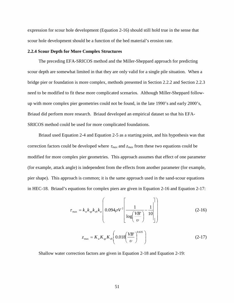
51

expression for scour hole development (Equation 2-16) should still hold true in the sense that

scour hole development should be a function of the bed material’s erosion rate.

2.2.4 Scour Depth for More Complex Structures

The preceding EFA-SRICOS method and the Miller-Sheppard approach for predicting

scour depth are somewhat limited in that they are only valid for a single pile situation. When a

bridge pier or foundation is more complex, methods presented in Section 2.2.2 and Section 2.2.3

need to be modified to fit these more complicated scenarios. Although Miller-Sheppard follow-

up with more complex pier geometries could not be found, in the late 1990’s and early 2000’s,

Briaud did perform more research. Briaud developed an empirical dataset so that his EFA-

SRICOS method could be used for more complicated foundations.

Briaud used Equation 2-4 and Equation 2-5 as a starting point, and his hypothesis was that

correction factors could be developed where τmax and zmax from these two equations could be

modified for more complex pier geometries. This approach assumes that effect of one parameter

(for example, attack angle) is independent from the effects from another parameter (for example,

pier shape). This approach is common; it is the same approach used in the sand-scour equations

in HEC-18. Briaud’s equations for complex piers are given in Equation 2-16 and Equation 2-17:

−

=101

'log

1094.0 2max

υ

ρτ α VBVkkkk shspw (2-16)

=

635.0

max'018.0

υVBKKKz shspw (2-17)

Shallow water correction factors are given in Equation 2-18 and Equation 2-19:

52

62.1/62.1/

1

85.034.0

><

=BHBH

BH

K w (2-18)

BH

deepw ek

4

)max(

max 161−

+==τ

τ (2-19)

where H is the height of the water and B is the width of the piers. For the case of closely spaced

piers, the spacing correction factors are given by Equation 2-20 and Equation 2-21:

( )nBWW

K sp −=

1

1 (2-20)

BS

sp ek1.1

)singlemax(

max 51−

+==τ

τ (2-21)

where W1 is the width of the channel without the piers n is the number of piers, and S is the

spacing between piers. For the case of different shaped piers, the shear stress correction factor is

given by Equation 2-22 where L is the width of the pier. The scour depth correction factor is

given by HEC-18. Briaud’s tests were on square-nosed piers, so he used a Kh value of 1.1. For

piers of other shapes, Briaud recommends using the same Kh factors prescribed in HEC-18.

BL

sh ek4

715.1−

+−= (2-22)

Finally, for the case of flow from a different angle, α, Briaud used the pier projected width, B’,

(the same B’ as in HEC-18) to evaluate this condition. Even with B’ defined however,

introduction of an attack angle coefficient, kα was still necessary for shear stress:

+=+= αααα cossincossin'

BLBBLB (2-23)

57.0

degree) (0max

max

905.11

+==

ατ

ταk (2-24)

53

2.3 Analytical Methods for Determining Erosion Rate-Shear Stress Relationships

Based on the preceding discussion on the aforementioned semi-empirical methods and

Slagle’s 2006 argument regarding the CSU equations, in recent years research has looked not to

define the scour-hole proper as a function of bed material, but rather use either a method similar

to the Miller-Sheppard approach or the EFA-SRICOS approach as a standard for overall scour

depth and fit one of these two models to a generalized scour scenario. At their core, these two

models require the same input parameter – an erosion rate vs. shear stress relationship. Logically

then, the goal of research should not be to define scour depth, but it instead should be to define

an erosion rate-shear stress relationship and if possible, generalize this relationship to other

geotechnical parameters.

There are two methods to determine this erosion rate-shear stress relationship. On one

hand, as discussed in the last section, engineers can take Briaud’s approach and try to fit

analytical sediment transport models to the problem. There is a significant advantage to this

approach. These models are based on physics and analytical reasoning, and as such, results from

these models can be used in a generalized scour situation for any bed material in which the

models’ assumptions are valid. In this section, a brief analysis will follow of several analytical

models, while in Section 2.4 analysis of the other method for determining an erosion rate-shear

stress relationship will be discussed – measuring this parameter directly using an erosion rate-

shear stress testing device.

2.3.1 Particle-Like vs. Rock-Like Erosion and Shields (1936)

In 1936, Shields argued that for a coarse sediment, there should be a shear stress, τc that

would represent the shear stress that caused incipient motion of bed material. This shear stress

could be drawn as a function of bed roughness, or the roughness Reynolds Number, Re* such

that:

54

( ) ( )*Ren

s

c fgd

=− ρρ

τ (2-25)

νdu*

*Re = (2-26)

ρτ cu =* (2-27)

Although Shields’ original data only corresponded to sands, over the years (following

Mantz 1977), his data points have been extended to cover the fine sediment regime (Figure 2-8).

The essential component of Shields’ work is his critical shear stress assumption. Shields

assumed that during an erosion event, erosion would only be caused by a small tug or pull on a

few particles on a material lattice. It can be shown that if this is the case, erosion must

correspond only to the Shields parameter given in Equation 2-25. This erosion mode will be

defined as particle-like erosion.

For non-cohesive sediments, this is true, but for cohesive sediments and rock, another

erosion mode exists. For cohesive material such as sand-clay mixtures and stiff rock-like

materials, this slight tug or pull on the exterior rock-like face sometimes does little in terms of

net-overall erosion. Rather, erosion under these conditions is instead governed by the fluctuating

normal force component on the material’s face and localized density/roughness/cracking in the

rock or sand-clay lattice.

When Miller used analytical sediment transport equations to calibrate his model, he only

considered the particle-like erosion mode. Under rock-like conditions, it may not be possible to

find erosion rate as a strict function of shear stress. Under this scenario, Equation 2-12 is still

valid, while Equation 2-16 is not because it would not be possible to define a sediment transport

constant when the governing component of sediment transport was a normal forcing parameter.

55

Still, for certain sand-clay mixtures, certain cohesive sediments, and some rock-like materials,

particle erosion is present, and methods for finding both critical shear stress and sediment

transport functions (erosion rate-shear stress relationships) should be discussed in some detail.

First, critical shear stress will be discussed, then methods for determining erosion rate-shear

stress curves will be examined.

2.3.1.1 Einstein (1943) and Christensen (1975)

In 1943, Einstein developed an expression for critical shear stress, τc of a cohesive bed

material based on a stochastic method (Einstein 1943):

( ) excrc dγγθτ −= (2-28)

where de is the effective grain size, γs is the specific weight of the sediment, γ is the specific

weight of water, and θcr is the Shield’s parameter, or parameter for incipient motion. Although

Einstein developed his own Shield’s parameter, in 1975, Christensen modified Einstein’s

equation and developed Equation 2-29 based on a probability distribution for erosion:

( )22

2

2

1

11

4.101ln556.0cot

1

u

ucr nS

r

S+

++

+=

ϕαα

θ (2-29)

where r is the roughness/grain-size ratio defined as the equivalent sand roughness, ks divided by

de, Su is the dimensionless value of the standard deviation of the velocity fluctuation, σ defined

by σu/ubar, ubar is the average velocity, n is the normalized velocity fluctuation u’/su, u’ is the

velocity fluctuation component, and α1 and α2 are shape factors. Christenson found that Su =

0.164 and n = 3.09 which corresponded to the probability of erosion Pr = 0.001 which was

related to the Gaussian distribution of u’ (Mehta 2007).

56

2.3.1.2 Wiberg and Smith (1987)

Wiberg and Smith developed their own relationship for critical shear stress in the late

1980’s. Their expression centered around the argument that when dealing with a mixed bed,

there are two length scales that need to be dealt with – the diameter of particle size that will be

eroded and the roughness of the surrounding bed. In other words, when dealing with a

heterogeneous bed, a smaller particle may erode first, but the flow velocity is dependent on the

size of the larger particles surrounding the smaller particle. To grapple with this scaling

problem, Wiberg and Smith introduced a Φ factor into their equations because they argue that

the particle failure angle changes for a mixed bed. In other words, it would be easier for a large

particle to roll over a bed that consisted of smaller particles than it would be for a small particle

to roll over a bed that consisted of larger particles (Barry 2003). An expression from Miller and

Byrne (1966) was used to quantify Φ. Wiberg and Smith’s critical velocity equation and Φ

equation are given by:

Φ+

−Φ

=

tan1

sincostan12

0

23

D

L

bb

Dcr

FF

zzf

Cθθ

ατ (2-30)

1/

/cos 01

++

=Φ −

s

s

kdzkd (2-31)

Where a3 is a parameter for grain geometry, f2(z/z0) is derived from the expressions for drag and

lift coefficient (Equation 2-32 and Equation 2-33), z is the height above the bed, z0 is the bottom

roughness parameter, qb is the bed slope, d is the particle diameter, and ks is the length scale for

bed roughness.

AuCF DD

2

21 ρ= (2-32)

57

AuCF LL

2

21 ρ= (2-33)

In these expressions, A is the cross-sectional area of the particle, CL is the lift coefficient, CD is

the drag coefficient, and ρ is the density of water.

To find the bottom roughness parameter, an expression for the velocity profile is

necessary. Wiberg and Smith used Reichardt’s 1951 expression which gives a transition

between the viscous sub-layer and the logarithmic flow above (Schlichting 1979, Barry 2003).

( ) ( )

−−−+=

++ −+

−−+ zz ezeczuzu 33.06.11* 6.11

11ln1 κκ

(2-34)

xkzRzu

z *0* ==+

ν (2-35)

skzRzu

z 0*0*0 ==+

ν (2-36)

υ

skuR *

* = (2-37)

where ν is the kinematic viscosity of water and R* is the roughness Reynolds Number.

2.3.1.3 Dade and Nowell (1991)

Dade and Nowell sought to develop a relationship for critical shear stress for a cohesive or

mixed bed that was independent of inter-particle cohesion forces (Barry 2003). Their expression

for critical shear stress is given in the Equation 2-38:

( ) ( )

−+

−

Φ−+Φ

Φ= 11cos131

240tan'

tan40

2

23

2

2

dgdg

d s

bscr ρρ

τρυ

ρρυτ (2-38)

where τb is the mud interfacial mud shear stress, g is the acceleration due to gravity, Φ was found

to be 65o, and previous terms have already been defined.

58

2.3.1.4 Dade et al. (1992)

The purpose of this investigation was to find an expression for critical shear stress that

included the effects of cohesion. This approach was similar to Weiberg and Smith’s approach

except that Dade et al. included a cohesion term. The resulting expression for the Shield’s

parameter is given in the following equations:

2

1

134

tan51

−

−−

ΦΞ=

XXX

crθ (2-39)

( )

2

3

ρνρρ dg s −

=Ξ (2-40)

Φ

+Ξ= 3

1

tan4800

1bW

FX

b

A π (2-41)

where b1 is a shape factor, Z is the Yalin (1972) parameter FA is the magnitude of the inter-

particle force, and Wb is the immersed weight of the particle grain. The ratio of immersed weight

to inter-particle force is obtained from Equation 2-42 (Barry 2003):

( ) ( )dgb

WF

s

y

b

A

ρρτ

−Φ−= cos13 2 (2-42)

2.3.1.5 Mehta and Lee (1994)

In 1994, Mehta and Lee developed their own relationship for critical shear stress by using

a balance between angle of repose, drag force, buoyant weight, and lift force as their starting

point rather than using the F factor that was employed by Christensen and Dade et al. Their

starting point, equation 2.3-19 led to the development of Equation 2-43 for critical shear stress:

` Lcb

D

FFWF

++=ϕtan (2-43)

59

( )( )

( ) 321

21

3 tantantan

tandg

Fdg s

c

s

c

ρρϕααϕ

ϕααϕα

ρρτ

−+

++

=−

(2-44)

( )βφφατ acax −= 4 (2-45)

Equation 2-45 was developed from an evaluation of previous laboratory tests where α4 and β are

sediment-specific constants. The advantage of this approach is that the Shields parameter is

easily recognizable on the left hand side of the equation.

2.3.1.6 Torfs et al. (2000)

Torfs took equation 2.3-19 from Mehta and Lee and noticed that it was only applicable for

erosion of a bed material of single-sized particle grains. Torfs sought to characterize entrainment

within a fine-coarse sediment mixture by size, dm and density, ρs. Everything else remains the

same as it did in equation 2.3-19, except that the cohesive force, Fc must be replaced with Fm, or

the force representing the effects of both cohesion and the influence of inter-bedded grains. The

result is:

( )( ) ( ) ms

ms

vcv

cgcgcg

cgcgc dg

dgK ρρ

ρρφφζ

φααφα

τξ

−

−−

++

='

tantan

21

3 (2-46)

where φvc is the fine solids volume fraction, φv is the threshold value of φvc below which the bed

becomes fluid-like, ξ and ζ are coefficients that depend on bed composition and levels of

consolidation, and a3 is the shape factor related to dm. dm is the characterization diameter,

analogous to the effective diameter, D* from the FDOTBSM except that dm refers to particle size.

The critical aspect of this equation is the inclusion of K’ which is included to quantify increases

or decreases in critical shear stresses due to the presence of fine materials. If K’ = 0, it implies

that there are no fine materials; an increasing K’ signifies a greater presence of fine materials and

a corresponding higher critical shear stress.

60

2.3.1.7 Sharif (2002)

In 2002, Sharif developed his own model for critical shear stresses of cohesive soils.

Sharif concluded that developing an all-inclusive model was not practical and instead, in his

work three different models were created. The first model was for pure clays, the second model

was for mixed beds with low clay content and the third model was for mixed beds with high clay

content.

For the case of a mixed bed with high clay content, Equation 2-47 provides an expression

for critical shear stress. In this equation, ρsn is the density of the non-cohesive particle, ρsc is the

density of cohesive particles, dnc is the diameter of non-cohesive particles, fc is the weight

fraction of cohesive particles, ρd is the bulk density of the bed, ξ is the magnitude of the force

between cohesive and non-cohesive particles, θ is the Shields parameter, dc is the average

diameter of cohesive particles, αvc and αvn are shape factors for cohesive particles, and αsn is an

area shape factor for non-cohesive particles.

( )3

222

18

−

+−=dnsn

sndc

sccnvnvc

snnsncn f

fdd

dgρρ

ρρρρπαα

ξθαθρρτ (2-47)

Equation 2-47 was developed by setting up a force balance between a single non-cohesive

particle and a cohesive sediment bed. The equation for critical shear stress of a pure clay bed,

Equation 2-48, was developed by creating a force balance for separation of aggregates from the

bed itself. In this equation, ρag is the density of aggregates, ζ is the average force between

cohesive particles, θ is the Shields parameter, and k1 and k2 are coefficients based on floc

diameter.

( ) sccvc

agk

agca d

gkρπα

θξρρρθτ 21

1 182

+−

= − (2-48)

61

Equation 2-49, the model for mixed beds with low clay content, was developed under the

assumption that critical shear stress under these conditions would be dominated by non-cohesive

particles and aggregates. Then, Sharif assumed that each component of critical shear stress – the

aggregate component and the non-cohesive component – would govern critical shear stress based

on the average area along the failure plane covered by each of these materials.

ab babca

bnbcnch AA τττ += (2-49)

where Anb is the area of non-cohesive particles,, Aab is the area of cohesive aggregate, and bn and

ba are experimentally determined coefficients.

2.3.1.8 Critical shear stress discussion

The previous section was a brief summary of a number of expressions that can define the

critical shear stress for a bed material analytically. This critical shear stress parameter is useless

as means of estimating scour depths if it cannot somehow be correlated to erosion rate. This

advance forward began in the 1960’s with Partheniades and has been improved since then.

2.3.1.9 Partheniades (1962)

In the early 1960’s Partheniades was conducting tests on mud from San Francisco Bay, and

he noticed that cohesive sediment eroded much differently from non-cohesive sediment.

Partheniades discovered that unlike sand, equilibrium scour depths are not reached when live-

bed conditions develop. In other words, with sand, eventually a scour hole gets to the point

where rate of deposition equals rate of erosion as sand particles are eroded and redeposited

within the domain of the hole. Mud on the other hand appears to harden until eventually the floc

shear strength can withstand the shear stress that is applied to it.

62

Using this rationale, Partheniades took the stochastic approach used by Einstein to develop

a relationship for critical shear stress. The resulting equation, Equation 2-50, gives erosion rate

as a function of bed shear stress (Figure 2-9).

−=−

−−

2

21

2

221erf

211 b

b

k

kkE

τ

τ

ω (2-51)

where erf is the error function, and k1 and k2 are experimentally determined coefficients that

equal 0.036 and 1.61 respectively (Mehta 2007).

In 1974, Ariathurai used empirical data to develop Equation 2-51, which is a straight-line

approximation of the trend shown by the Partheniades equation (Figure 2-9).

( )cbME ττ −= (2-51)

This equation is extraordinarily significant because of its overall form. Equation 2-51 shows

that for a cohesive bed material under particle-like erosion conditions, erosion rate should be a

function of the deficit between critical shear stress and bed shear stress – or the same form that

Miller saw during his analysis.

2.1.1.10 Christensen (1975)

In parallel with his work on critical shear stresses for cohesive beds, Christensen also

developed an expression for average shear stress on a sediment bed:

+=22

12 u

uC uDb

σρτ (2-52)

2.3.1.11 McLean (1985)

In 1985, McLean developed an energy balance between potential energy of an entrained

particle and bed shear stress. This resulted in an expression for erosion rate of eroding bed

particle, or Equation 2-53:

63

c

cbeME

τττ −

= (2-53)

According to Mehta, this relationship was actually first proposed by Kandiah (1974) based solely

on empirical results. This equation also resembles the Partheniades equation and the Ariathurai

equation, and serves as further evidence that quantifying erosion rates as a function of shear

stress should be a valid method for predicting scour depths under particle-like conditions.

2.3.1.12 Van Prooijen and Winterwerp (2008)

In 2008, Van Prooijen and Winterwerp argued that knowledge regarding the stochastic

nature of the turbulent boundary layer has increased. Therefore, the probability density function

(PDF) is now known more accurately than before when Einstein, Christensen, and others were

conducting their research. Using the same approach as Hofland and Battjes (2006) and data from

Obi et al. (1996), a new PDF was developed for bed shear stress:

( )

−−= δ

π

α *

* 21exp

22)( T

TTp (2-54)

where T is given by the dimensionless parameters:

u

buσ

ω = (2-55)

u

uuσ

δ = (2-56)

||2 ωωρστ

==u

bT (2-57)

|2* βδα −= TT (2-58)

and ω is the dimensionless near-bed velocity, δ is the dimensionless mean velocity, and T is the

dimensionless shear stress. Parameters are scaled with σu or the standard deviation of near-bed

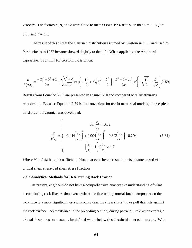
64

velocity. The factors α, β, and δ were fitted to match Obi’s 1996 data such that α = 1.75, β =

0.83, and δ = 3.1.

The result of this is that the Gaussian distribution assumed by Einstein in 1950 and used by

Partheniades in 1962 became skewed slightly to the left. When applied to the Ariathurai

expression, a formula for erosion rate is given:

+−

−++

−+−

++

++−=

22erf

21

22exp

221 **22

***2* δ

αδδδ

παδ

αδ

ρσcc

cccc

u

TTTTTTM

E (2-59)

Results from Equation 2-59 are presented in Figure 2-10 and compared with Ariathurai’s

relationship. Because Equation 2-59 is not convenient for use in numerical models, a three-piece

third order polynomial was developed:

>

−

+

−

+

−

<

=

7.1 if 1

204.0823.0904.0144.0

52.0 if 0

23

c

b

c

b

c

b

c

b

c

b

c

b

cME

ττ

ττ

ττ

ττ

ττ

ττ

τ (2-61)

Where M is Ariathurai’s coefficient. Note that even here, erosion rate is parameterized via

critical shear stress-bed shear stress function.

2.3.2 Analytical Methods for Determining Rock Erosion

At present, engineers do not have a comprehensive quantitative understanding of what

occurs during rock-like erosion events where the fluctuating normal force component on the

rock-face is a more significant erosion source than the shear stress tug or pull that acts against

the rock surface. As mentioned in the preceding section, during particle-like erosion events, a

critical shear stress can usually be defined where below this threshold no erosion occurs. With

65

rock and materials that obey rock-like erosion characteristics, this shearing threshold does not

appear to exist. There has been limited analytical work completed in this area, and most of it is

still unable to accurately predict erosion rates.

2.3.2.1 Cornett et al. (1994) and Henderson (1999)

According to Cornett et al. (1994) and Henderson (1999), erosion of rock may not be

directly related to shear stress because erosion occurs along a rock’s internal fracture plane, and

this may be driven by hydrodynamic pressures within the fracture. Figure 2-11 was proposed by

Cornett, Henderson, and Kerr (2001) as a possible explanation for erosion of rock. In this

sketch, the crack, which is a stagnation point, of length l and height t is subjected to a steady

flow of velocity u. Bernoulli’s equation can be applied to this scenario such that the pressure

difference between the crack and the external flow can be expressed:

( )2

22

212

221

ugtuuP ρρ≈+−=∆ (2-62)

This pressure differential is the velocity head that acts to open the crack, and fracture

occurs when the pressure within the crack exceeds rock strength. The bending moment, M in the

rock above the crack base can also be written (Equation 2-63), and the maximum axial stress to

carry the moment can be expressed (Equation 2-64) (Henderson 1999).

42

21

22 ulPlM ρ=∆= (2-63)

2

1max 5.1

== t

luρσ (2-64)

Equation 2-64 implies that to failure resistance is proportional to the square of free-flowing fluid

velocity. Note that this expression deviates from the shear-based expressions presented in

Section 2.3.1.

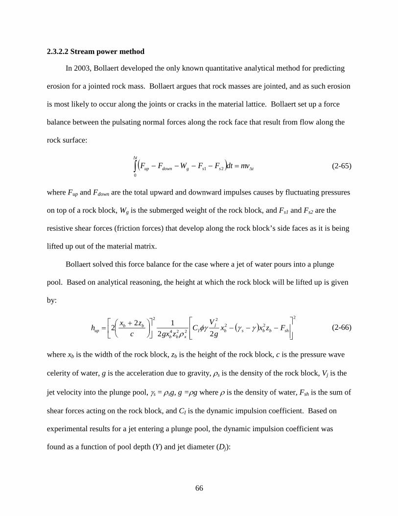
66

2.3.2.2 Stream power method

In 2003, Bollaert developed the only known quantitative analytical method for predicting

erosion for a jointed rock mass. Bollaert argues that rock masses are jointed, and as such erosion

is most likely to occur along the joints or cracks in the material lattice. Bollaert set up a force

balance between the pulsating normal forces along the rock face that result from flow along the

rock surface:

( ) t

t

ssgdownup vmdtFFWFF ∆

∆

∫ =−−−−0

21 (2-65)

where Fup and Fdown are the total upward and downward impulses causes by fluctuating pressures

on top of a rock block, Wg is the submerged weight of the rock block, and Fs1 and Fs2 are the

resistive shear forces (friction forces) that develop along the rock block’s side faces as it is being

lifted up out of the material matrix.

Bollaert solved this force balance for the case where a jet of water pours into a plunge

pool. Based on analytical reasoning, the height at which the rock block will be lifted up is given

by:

( )2

222

224

2

22122

−−−

+

= shbbsbj

Ixbb

bbup Fzxx

gV

Czgxc

zxh γγφγρ

(2-66)

where xb is the width of the rock block, zb is the height of the rock block, c is the pressure wave

celerity of water, g is the acceleration due to gravity, ρs is the density of the rock block, Vj is the

jet velocity into the plunge pool, γs = ρsg, g =ρg where ρ is the density of water, Fsh is the sum of

shear forces acting on the rock block, and CI is the dynamic impulsion coefficient. Based on

experimental results for a jet entering a plunge pool, the dynamic impulsion coefficient was

found as a function of pool depth (Y) and jet diameter (Dj):

67

2.1119.00035.02

+

−

=

jjI D

YDYC (2-67)

Based on these equations, one can compute the height to which an eroding rock mass will

move from its matrix. If the ratio between hup and zb is greater than 1.0, the rock segment will

likely erode. If this ratio is between 0.5 and 1.0, the rock may erode or it may not depending on

ambient flow conditions. If this ratio is between 0.1 and 0.5, the rock block will probably vibrate

but remain in place and not erode. If this ratio is less than 0.1, the rock block will remain in

place.

Bollaert intended this model to be used under conditions similar to a dam spillway.

However, it may be possible to develop a similar model for use under local scour conditions.

When local scour is present, the force balance shown in equation 2.3-40 is the same as it would

be when water is entering a plunge pool. The vertical forces are caused by the horseshoe

vortices instead of the jet velocity while the resistive forces remain the same. If this is the case,

then it appears as though the fluctuating normal stress impulse along a rock’s surface during a

local scour event should play a role in determining the rock’s erosion rate.

2.4 Empirical Methods for Measuring Scour and Erosion in Cohesive Soils and Rock

Most of these aforementioned analytical expressions for erosion in cohesive soils and rock

contain a high number of governing parameters. Trammel (2004) argues that it is unrealistic to

develop accurate predictive correlations based on these variables. Trammel also cites Mehta

who says that the cost of evaluating this high number of parameters is often prohibitively high.

Because of this, Trammel argues that pure empirical methods for predicting erosion rate-shear

stress relationships should be explored. Slagle (2006) agrees with Mehta’s and Trammel’s

assessments, and he also advocates the use of pure empirical erosion rate-shear stress

68

relationships for use in the EFA-SRICOS or a method similar to the Miller-Sheppard scour

models.

2.4.1 Erosion Rate-Shear Stress Standards for Rock

HEC-18, the state-of-the-art in rock erosion and rock scour is empirically based, but even

still most results in this design manual are strictly qualitative. A series of simple guidelines are

presented where an engineer can pseudo-determine whether or not a given rock or rock-like

material will erode. Specifically, four categories of analysis are recommended to qualitatively

determine how a rock-face will react to changing flow conditions resulting from a foundation

(Richardson and Davis 2001):

1. Geologic, geomorphologic, and geotechnical analyses 2. The July, 1991 memorandum from the FHWA titled “Scourability of Rock Formations” 3. Flume tests to determine the resistance of rock to scour 4. Erodibility Index procedure

2.4.1.1 Geologic, geomorphologic, and geotechnical analyses (Richardson and Davis 2001)

To determine the geologic parameters used for design, HEC-18 says that extensive rock

coring should be used. The cores should be subjected to standard field classification and soil

mechanics tests. The geologic formation on which the bridge is to be constructed needs to be

determined and mapped. The geomorphology of the site needs to be determined and related to

the erodibility of the foundation material. The long-term stability of the stream or waterway

needs to be estimated, studied, and related to these geomorphological parameters. Additionally,

erosion should be made if the erodibility or scourablity of the rock is unknown.

2.4.1.2 July 1991 FHWA “Scourability of Rock Formations” (Gordon 1991)

According to Trammel, because numerous bridge foundation failures have occurred as a

result of rock or rock-like scour, in 1991, the FHWA developed an interim guidance document to

assess rock scourability by using empirical methods and testing procedures. Trammel says that

69

these procedures are provided as a guideline until results from ongoing research permit more

accurate evaluation procedures for estimating a design scour depth (Gordon, 1991 and Trammel

2004).

According to the memorandum, no single rock index property will properly predict

whether or not a rock will scour. Rather, different rock scours for different reasons. For

example, a rock may have a high bearing capacity and be very hard, but when water passes over

it, it may erode rather quickly. The memorandum encourages designers to use a combination of

the following seven methods to assess scourability until more qualitative procedures become

available (Gordon 1991):

1. Subsurface Investigation 2. Geologic Formation/Discontinuities 3. Rock Quality Designation (RQD) 4. Unconfined Compressive Strength, qu 5. Slake Durability Index (SDI) 6. Soundness 7. Abrasion

Subsurface investigation. The subsurface investigation portion of the memo simply

provides guidelines for the type of borehole pattern to be used when preparing to build a bridge

foundation. At minimum, a 3.3 m core length of material below the footing should be obtained

and subjected to the remaining six examinations (Gordon 1991).

Geologic formation/discontinuities. In general, the 1991 memo says that rock cores with

one or fewer fractures per foot should indicate that the rock is of good quality and may resist

scour. High rock fracture rates (five or six fractures per foot) qualitatively appear to indicate a

poor quality rock that may be scourable (Gordon 1991).

Rock quality designation (RQD). RQD is a modified computation of percent rock core

recovery that reflects the relative discontinuity of the rock. The 1991 memo says that rock cores

70

with an RQD less than 50 should be considered to be soil-like and therefore at a high risk of

scour (Gordon 1991).

Unconfined compression strength. According to the 1991 memo, qualitatively as

compressive strength, qu, increases, bearing capacity increases and scourability decreases. The

memo says that there is only a generalized correlation between scourability and compressive

strength.

Slake durability index (SDI). The SDI test is a test used on metamorphic rock and

sedimentary rock like slate and shale. In general, a low SDI number indicates a highly erodible

material. The 1991 memo says that an SDI value lower than 90 indicates that the rock could be

highly scourable (Gordon 1991).

Soundness. Soundness is measured by soaking the rock in a magnesium or sodium

sulfate solution for twelve hours. Generally, the less sound the rock, the more scourable it will

be, but specifically, the 1991 memo says nothing regarding what “less sound” means relative to

“more sound” (Gordon 1991).

Abrasion. The 1991 memo cites the Los Angeles Abrasion Test as the method to use for

measuring this parameter. Qualitatively, the less a material abrades, the less it will scour, and

materials with loss percentages greater than 40 should be considered highly erodible (Gordon

1991).

Discussion of 1991 Memorandum. The above-mentioned memorandum is highly

qualitative; there is no definitive point where an engineer can say that a material will or will not

erode based on the information given here. Further, this memo was released in 1991; it is nearly

twenty years old and there is not yet a better, more quantitative method for estimating or

establishing an erosion rate of a rock or rock-like bed material that can be used in design.

71

2.4.1.3 Erodibility index method (Annandale et al. 1996)

The Erodibility Index Method (ERI) was developed by Annandale, and it identical to

Kirsten’s Excavatability Index (Richardson and Davis 2001). It is used to quantify the relative

ability of a non-uniform earth material to resist erosion. Figure 2-12 provides a definition sketch

for the erodibility index method. Water along the bed experiences turbulence, and Annandale

suggests that this turbulence causes a pressure gradient that progressively “jacks” rock material

from its initial position. Once removed, the material then becomes dislodged and displaced.

In the ERI, a material’s ability to withstand erosion, Kh, which is identical to Kirsten’s

ripability index, is defined:

sdbsh JKKMK = (2-68)

such that Ms is the mass strength number, Kb is the particle or block size number, Kd is the

discontinuity or inter-particle bond strength, and Js is the relative ground structure number. The

mass strength number is determined from the material strength of an intact sample of rock

without regard to geologic heterogeneity. The particle or block size number is a factor that

represents the rock mass quality. The bond strength factor represents the relative strength of

discontinuities and it is made by visual observations. The ground structure number relates the

shape of material particles to the direction of free-stream flow (Henderson 1999)

Tests were conducted at the Turner Fairbank Highway Research Center’s (TFHRC)

Hydraulics Laboratory to find a relationship between stream power and scour depth so that a

practical application of the ERI could be used for scour prediction. HEC-18 says that based on

these tests, although a relationship between ERI and stream power appears feasible, more

research is still needed (Richardson and Davis 2001). This evaluation was made before

development of Bollaert’s Stream Power Model.

72

2.4.1.4 Flume tests (Richardson and Davis 1991)

Appendix M of HEC-18 says that samples should be subjected to flume tests to see if

they erode. This conclusion is interesting, as it is the same conclusion that is drawn from

Appendix L for cohesive sediments. Under cohesive scour conditions, the semi-empirical

approaches discussed in Section 2.3 may be applied, and in principle, these methods should be

usable when rock is present as well. This ultimately means that for either cohesive sediments or

rock, the same method – flume tests (or similar erosion rate testing devices) – are the most

effective solution for determining a material’s erosion rate-shear stress curve.

2.4.2 Erosion Rate Testing Devices

In principle, the idea of using a flume or a similar erosion rate testing devices appears as

though it should be straight-forward. However, like most variables pertaining to the scour

problem, implementation of a properly working erosion rate testing device is not as easy as it

sounds. The following is a summary of a number of erosion rate testing tests that have been

conducted in recent years. Although not every device mentioned was designed to capture

erosion rate-shear stress relationships specifically, this discussion highlights the evolution of

erosion rate testing devices.

2.4.2.1 Nalluri and Alvarez (1992)

In 1992, Nalluri and Alvarez ran a study to identify the influence of cohesive sediment on

erosion of a mixed bed. Tests were conducted in a 154 mm wide open channel and a 302 mm

diameter pipe. Their study led to three important conclusions. First, even a low level of

cohesive material (and subsequently cohesion) can increase the critical shear stress (and critical

velocity required to move a non-cohesive particle). Secondly, sand size has no effect on the

critical shear stress of a cohesive sediment. Third, for a given sand, an optimum sand-clay

mixture could be achieved where critical shear stress was maximized.

73

2.4.2.2 Mitchener and Torfs (1996)

In 1996, Mitchener and Torfs synthesized a series of laboratory data from a variety of

different types of erosion tests to try to quantify the erosion rates of sand-mud mixtures. After

analysis of these data sets, a number of interesting conclusions were drawn:

1. The addition of even a little bit of mud to sand affects the critical shear stress of the mixture.

2. If enough mud is added to sand, the entire mixture behaves as if it was a mud, and these results agree with earlier results by Dade and Nowell.

3. The addition of mud to clays also decreases the erosion rate of sand/clay mixtures compared to what the erosion rate would have been had the mud not been present. Inversely, the addition of sand to mud increases the erosion rate of the mixture.

4. A recommendation was made to further investigate the relationships between erosion parameters (critical shear stress and erosion rates) and bed roughness from 0% sand to 100% sand.

Mitchener and Torfs tried to develop a relationship between erosion rate and bulk density

and critical shear stress as well. This relationship is presented in Figure 2-13, while relationships

between erosion rate, shear stress, and critical shear stress are presented in Figure 2-14 and

Figure 2-15.

2.4.2.3 Panagiotopolous et al. (1997)

Panagiotopolous sought to further study the effects of clay content on a non-cohesive bed.

His results suggest that critical shear stresses increase with increased clay content while

erodibility decreases with increased clay content. He identified two specific regimes:

1. For sand/clay mixtures where there was less than 30% clay present, there is a slight increase in the critical shear stress for the bed material.

2. For sand/clay mixtures where there was more than 30% clay present, erosion rate decreases.

According to Barry (2003), these results agree with Dyer (1986) and Raudkivi (1990).

74

Additionally, this study found that if the critical stress was not exceeded for a sand/clay

mixture, or if u was less than uc, and then the velocity was to be slowly increased, critical shear

stress would also increase as a result of this pre-critical flow. This was expected because even

though the critical velocity was not met at these lower speeds, grains or aggregates that did not

satisfy the threshold criterion adjusted to more stable positions within the bed. The implication

here is that when tests are run in the EFA or the SERF, velocities need to be selected randomly

when erosion rates are measured. If velocities are not selected randomly, the erosion-rate testing

apparatus will under-predict the erosion rate for a given shear stress.

2.4.2.4 SEDFlume (McNeil et al. 1996, Jepsen et al. 1997)

In 1996, McNeil wanted to find the erosion rates and associated shear stresses of fine

grained bed materials. His motivation was environmental, not structural; his goal was to see if

there was there potential for contaminants at the bottom of rivers to resuspend themselves during

large-scale storm events.

To investigate this issue, McNeil developed the Sediment Erosion at Depth Flume or

SEDFlume. At the time, SEDFlume was unique because it allowed for in-situ testing of bed

materials. According to McNeil, previous laboratory designs by their nature disturbed the

sediment that they tested; McNeil cites Fukuda and Lick (1980), Mehta, et al. (1982), Tsai and

Lick (1988), and MacIntyre et al. (1990) as examples of laboratory flumes that disturb the

samples that they are testing (McNeil et al. 1996).

A sketch of the original SEDFlume schematic is presented in Figure 2-16. An undisturbed

sample is loaded into the SEDFlume and a piston is placed below the sample. Then, water was

pumped through the 2 cm by 10 cm flume from a 120 gallon reservoir tank. As the water passed

over the sample, the sample eroded, and as the sample eroded, the piston was raised so that the

sample was level with the bottom of the bed (McNeil et al. 1996). The mechanism for raising

75

the piston (and subsequently the sample) into the flume was operator dependent. The research

technician was charged with watching the sample erode and advancing the sample into the flume

with a 1/3 hp motor. One had to have experience using the device to know when to turn on the

motor, how fast to raise the piston, etc. Shear stresses in the SEDFlume were estimated using

Prandtl’s Universal Law of Friction. For a rectangular duct with smooth surfaces, Equation 2-69

can be derived:

8.0log0.21−

=

υλ

λUD

(2-69)

wh

hwD+

=2 (2-70)

2

8Uρτλ = (2-71)

where λ is the friction factor defined by the Darcy-Weisbach equation given in 2-71, U is the

freestream velocity, D is the hydraulic diameter defined by equation 2-70, ν is the kinematic

viscosity of water, h is the height of the duct, w is the width of the duct, and τ is the shear stress

on the four walls of the duct. These three equations can be combined to find shear stress as an

implicit function of freestream velocity. To measure freestream velocity, a paddlewheel

flowmeter was used (McNeil et al. 1996).

As shown here then, the SEDFlume did not measure shear stresses directly; rather, shear

stresses were implied as a function of freestream velocity. The assumption behind the usage of

these equations then is that the shear stress on the walls of the flume approximates the shear

stresses seen by the eroding sample and that the SEDFlume is hydraulically smooth. In his

paper, McNeil says that he uses a relationship between shear stress and flow rate for a

hydraulically smooth flow (Figure 2-17).

76

Measurements of erosion rates were conducted on a series of samples from the Trenton

Channel of the Detroit River from 1993 – 1994. McNeil organized erosion rates as a function of

both core depth and shear stress. McNeil’s results (Figure 2-18) show that as shear stress

increases, erosion rate also increases, and they imply another interesting phenomenon. As depth

increases for a given shear stress, it appears that erosion rates level off. Consider that McNeil

was dealing with cohesive sediments. As depth increases for a cohesive sediment, it is likely that

consolidation of these sediments increases. As consolidation increases, it is likely that material

strength, or cohesive strength, of the sediments increases. If this is true, then his results imply

that material strength also plays a role in determining the erosion rate of his bed materials.

In 1997, Jepsen, Roberts, and Lick extended McNeil’s work. They ran a series of tests to

determine erosion rate and critical shear stress as a function of bulk density for bed particles

from the Detroit River in Michigan, the Fox River in Wisconsin, and a slough near Santa

Barbara, California. Their results show that for a given shear stress, erosion rate is a unique

function of bulk density and erosion rate decreases as bulk density increases (Jepsen et al. 1997).

This appears to imply a further dependence between erosion rate and material strength because

as density increases, materials become more compacted. As materials become more compacted,

their cohesive strength should increase. Shear stress estimation still utilized a flat-bottom Darcy-

Weisbach frictional coefficient.

In 2003, the SEDFlume was enhanced so that it could produce oscillatory flows. The new

device was named the SEAWOLF and it was used to measure erosion rates of quartz sand under

these oscillating conditions. To predict shear stress under oscillating conditions, an effective

shear stress for wave motion is estimated. Then, this effective shear stress is transferred to

77

erosion rate-shear stress relationships from unidirectional flow to yield a prediction for erosion

rate under wave conditions (Jepsen et al. 2003).

2.4.2.5 ASSET (Roberts et al. 2003)

In 2003, Roberts et al. developed the second generation of the SEDFlume. The motivation

behind this research was that although the SEDFlume was useful for measuring sediment erosion

rate properties, it only measured bulk erosion rates. The SEDFlume gave no information

regarding the transport mode of eroded materials – i.e. bedload vs. suspended load. The

Adjustable Shear Stress Erosion and Transport (ASSET) Flume was designed to determine the

bedload fraction of eroding sands.

The ASSET was similar to the SEDFlume, but its dimensions were slightly larger. While

the SEDFlume was 2 cm tall by 10 cm wide, the ASSET was 5cm high by 10.5 cm high. The

ASSET was designed with a bedload trap positioned 1 m downstream from the eroding sample

(Figure 2-19). Sand caught in the bedload trap during a test was the bedload fraction from that

run (Roberts et al. 2003).

The ASSET used the same method as the SEDFlume for estimating shear stresses on an

eroding sample – equation 2.4-2, equation 2.4-3, and equation 2.4-4. Results from the ASSET

show that bedload fraction is a function of both particle size and shear stress (Figure 2-20).

Because the focus of this study was on determining bedload, no information was given regarding

total erosion rate as a function of shear stress.

Roberts mentions that some qualitative work was done in the ASSET with cohesive

sediments. Although no hard data is given in his paper, he notes that cohesive sediments often

do not erode as individual particles; rather, cohesive sediments erode as aggregates, or flocs

(Roberts et al. 2003).

78

2.4.2.6 EFA (Briaud et al. 1991-2004)

The EFA-SRICOS method has been discussed at length in terms of the initial requirements

necessary for its implementation. In preceding discussion regarding the EFA-SRICOS method,

it was assumed that it would be possible to determine a shear stress-erosion rate relationship.

The principle behind the EFA is similar to principles behind both the ASSET and the

SEDFlume. In fact, the EFA and the ASSET/SEDFlume/SEAWOLF apparatuses were

developed independently from one another. A sample is loaded into the flume through the

bottom, and as water passes over the sample, the sample is advanced into the flume. Through

this mechanism, erosion rate is measured directly.

Similar to the ASSET and the SEDFlume, the advancement mechanism of the EFA (Figure

2-21) was also conducted via visual inspection. According to the EFA testing procedure, the

sample is to be loaded into the flume such that it protrudes into the flume 1 mm (Figure 2-22);

presumably this protrusion into the flume is recommended so that visual inspection is easier.

As of the date of the last known EFA publication (2010), the EFA estimates shear stress by using

a Moody chart (Figure 2-23). Shear stress is approximated by finding a friction factor from the

Moody diagram and then using the friction factor to approximate shear stress with the following

equation:

2

81

ρντ f= (2-72)

where τ is the shear stress, f is the friction factor, ρ is the density of water, and ν is the kinematic

viscosity of the water.

Like other erosion rate testing devices, the EFA does have drawbacks, and erosion rate-

shear stress data from it has been criticized in the past. First, the EFA’s method for shear stress

estimation has been questioned (for example in Annandale 2005). Friction factor estimation

79

from the Moody Diagram depends on selection of the correct roughness factor or roughness

height. If the relative roughness of an eroding sediment can be properly estimated, the Moody

Diagram method may work properly, but selecting the correct relative roughness for a bed

material is not straight forward. In his work, Briaud does not indicate what value for relative

roughness he is using during EFA shear stress estimates, nor does he indicate how any roughness

coefficient is calibrated in his flume. Further, the Moody diagram was developed from tests with

pipes of uniform roughnesses. The EFA does not have a uniform roughness. The side walls and

top of the EFA’s rectangular duct are smooth while the false bottom in which the sample projects

itself into the flume is rough. Annandale (2005) says that because of this, using a uniform

roughness coefficient from a Moody diagram is incorrect.

The second possible oversight with regard to the EFA is that the sample protrudes into the

flume 1 mm. If the sample is protruding into the flume, it will be subjected to both normal

stresses and shear stresses. Because of the addition of a normal stress, the sample will erode

faster than it would if it was subjected to only a shear stress. It appears then that for a given

shear stress as estimated upstream using a Moody Diagram (or more explicitly a given velocity,

as velocity is the only quantity that is actually measured during the test), erosion rates would be

overestimated. This overestimation of erosion rates for a given shear stress would lead to

conservative equations. Conservative equations are better than non-conservative equations, but

if the erosion rate data from the EFA could be improved, it may be possible to avoid over

designs.

The third possible issue associated with the EFA-SRICOS method is the same discussed

with both the ASSET and the SEDFlume in that these devices rely on visual inspection to

80

advance the sample into the flume. They are also operator dependent, and reproduction of

results may be difficult.

2.4.2.7 RETA (Henderson 1999 Kerr 2001 and Slagle 2006)

Preceding erosion-rate testing devices that were used to estimate shear stresses and

measure erosion rates of cohesive material were designed similarly: a flume was used to flow

water over an advancing sample, and a theoretical relationship used to estimate the shear stress

on it. In 2001, The Rotating Erosion Testing Apparatus (RETA) was designed to measure

erosion rates and shear stresses of a intact bed material as an alternative design.

The RETA (Figure 2-24) approaches the problem differently than traditional bottom-

loaded flume designs. Instead of flowing water over a sample, in the RETA a sample is loaded

into an annulus filled with water (Figure 2-25 and Figure 2-26). The annulus spins around the

sample which creates a shear stress, which in turn causes the sample to erode (Figure 2-27).

Before the sample is loaded, a hole is drilled through it, a rod is attached through the center of

the sample, and the sample rod is attached to a torque cell (Figure 2-28). Rather than inferring

shear stress from theoretical equations that describe shear stress on the flat walls of a flume, the

torque cell measures the shear stresses directly (Kerr 2001).

The torque cell measures torque on the entire sample as the rotating cylinder spins around

it. To convert the torque measurement to shear stress, Equation 2-73 is used. To find the total

erosion rate, Equation 2-74 is applied. In these equations, R is the radius of the sample, L is the

length of the sample, T is the torque measured from the torque cell, E is the erosion rate, ∆m is

the amount of mass removed during the test, and D is the duration of the test. Standard RETA

tests are specified to be run for 72 hour increments (Sheppard et al. 2006).

LR

T22

StressShear Averageπ

τ =≡ (2-73)

81

RLDmE

πρ2∆

= (2-74)

The most obvious advantage to RETA testing is that shear stress is measured directly, but

this technique is not without criticism. Because the gap between the sample and the annulus’

walls is small, the size of turbulence-induced vortices in the flow regime between the sample and

the annulus wall may be different for the same average shear stress. In other words, under rock-

like erosion conditions where the normal force impulse to the rock face is the dominant erosion

mode, the fluctuating normal stress component to the material face will be different than it would

be in nature.

There are other pitfalls in using average shear stress along a vertical plane to represent the

shear stress on the sample. The RETA presumes uniform erosion; in reality, when rock is

subjected to RETA testing, sometimes chunks of the material often erode at one time. This

“chunking” and “pitting” mechanism can produce localized shear or normal stresses along the

sample face that are higher than the uniform component. This is in turn can produce more

chunking, which in turn can produce even greater localized shear stresses, etc. These localized

stresses cause localized higher erosion rates, yet a value for average erosion rate is the goal.

Because erosion rate is measured by simply measuring the mass of the sample at the end of the

test and subtracting this mass from the total mass at the beginning of the test, these localized

variations can cause inaccurate average erosion rate results.

This pitting or chunking mechanism implies the presence of rock-like erosion, and while

shear stress is measured directly in the RETA, normal stress is not. As shown in Section 2.3,

when rock-like erosion dominates, erosion rate is probably not a strict function of shear stress.

The third criticism with the RETA is that because the fluid around the sample is being

spun, the sample is subjected to torque or moment action. Kerr (2001) and Slagle (2006) both

82

argue that this behavior would lead to slightly more conservative equations and is therefore

acceptable. Critics, particularly those who would label the equations in HEC-18 as “overly

conservative” would argue that because there is no quantitative date to support the claim that this

moment action leads to only “slightly conservative results,” one cannot be sure how overly

conservative the RETA is (Kerr 2001). Because of these concerns, there has been a goal in recent

years to correlate RETA results to results from another erosion-rate testing apparatus.

RETA Results. Tests in the RETA were conducted by both Kerr in 2001 and Slagle in

2006. Kerr’s tests were preliminary; the focus of his work was development and calibration of

the instrument. Slagle’s work on the other hand was more comprehensive. First, Slagle

conducted a series of RETA tests on limestone taken from the Jewfish Creek Bridge on US 1 in

near Key Largo, FL. Like Briaud, Slagle developed curves for erosion rate vs. shear stress

(Figure 2-31). However, Slagle, after discussion with Bloomquist, hypothesized that erosion rate

of a rock may also be a function of material strength. He presented one graph of particular

interest (Figure 2-32) in his Master’s Thesis that shows Jewfish Creek limestone behaving with

some dependence on cohesion.

Cohesion may be derived from two Mohr’s Circle using simple geometry (Figure 2-33). If

one examines triangle zqy, the cosine of the angle, θ, and the sin of the angle can be defined:

12

12cosRRRR

+−

=θ (2-75)

12

212sin

RRRR

+=θ (2-76)

If a perpendicular line is then drawn from point x perpendicular to the x-axis, a new

triangle will be apparent, and the length of the perpendicular distance from point x to the x-axis

83

can be shown to be R2sinθ. Furthermore, the slope of line wx must be the same as the slope of

line zq, and it must equal –xcotθ.

Next, coordinates are transferred such that the new y-axis now sits at the center of Circle 2.

From above, the equation of line wx through the new coordinate system must be:

θθ

cotsin

' 2 xR

y −= (2-77)

Cohesion is defined as the point where line wx, the line tangent to both the Mohr’s Circle for

axial strength (circle 1) and the Mohr’s Circle for compressive strength (circle 2) crosses the x-

axis. Setting x in Equation 2-77 equal to R2 and using Equation 2-75 and Equation 2-76 yields

the following expression:

21

12'RRRR

y = (2-78)

Substituting qu and qt, or the compressive and axial strength definitions respectively, yields:

tu qqCy21

=≡ (2-79)

where C is the cohesion.

Figure 2-32 appears to indicate that erosion rate may be a function of shear stress and

cohesion, but Slagle’s results are limited. This figure is the only graph that he presents that

shows this relationship. More work needs to be done to determine if this dependence on

cohesion is simply a coincidence that was found for Jewfish Creek Limestone or if this

dependence on cohesion can be extrapolated to other materials. Work by Briaud et al. (1999)

suggests that erosion rate is not a function of any geotechnical properties and therefore he

recommends his site-specific EFA-SRICOS method. In a 2002 discussion piece, Hanson and

Simon agree with Briaud’s assessment (Hanson and Simon 2002).

84

On the other hand, if one examines the definition of a Mohr’s circle, the vertical axis

represents shear stress while the horizontal axis represents normal stress. If erosion is caused by

a simple shearing action, then the normal stress – or value along the Mohr’s circle x-axis –

should be close to zero. This would lead directly to the y-intercept, or the cohesion point. If

Slagle’s apparent relationship between erosion rate and cohesion can be proven, it may

contradict Briaud’s assessment and provide an alternative means for predicting erosion rates of

bed materials. Slagle’s relationship implies that under the conditions that he studied, shear stress

was dominant.

Slagle’s other results from the RETA focused at finding erosion rates of Gator Rock

(Section 2.5). For now, it is sufficient to say that Gator Rock is a material that is designed to be

uniform in its properties. Slagle did this run of tests presumably to compare RETA results with

SERF (Section 2.4.2.9) results, but instead of running the same shear stresses in each instrument,

he used the RETA to measure results with a low shear stress and the SERF to measure results

with a high shear stress.

Slagle argued that because his erosion rate curves followed the same trends when he

combined instrumental results, it proved that both instruments were measuring erosion rate and

shear stresses correctly and that the RETA had been verified. This argument is questionable

because there are significant “gaps” between the data sets. For example (Figure 2-34), there are

no readings between approximately 40 Pa and approximately 70 Pa.

This data gap is typical for most of Slagle’s tests. Slagle only ran one test where there was

an overlapping shear stress data point. Although this data point did match in both the RETA and

the SERF, one point is not enough to say that results from the RETA are proven to be the same

as they would have been using a more traditional erosion rate testing device. Slagle also

85

discussed issues with Gator Rock non-uniformity in his thesis. Although a graph of Gator Rock

erosion is presented here, there no data could be found that verified near uniform erosion in the

RETA. As discussed, a fundamental assumption behind the RETA is that samples will erode

uniformly; if they do not, it is difficult to rely on the results, and hard to say what is being

measured.

2.4.2.8 Barry et al. (2003)

In 2003, Barry ran a series of tests to determine how critical shear stress of a sand-clay

mixture varied based on clay content. Testing was conducted in a recirculating flume, a Schultz

ring tester, and a RETA (although as of 2003, the RETA was called the “Simulator of Erosion

Rate Function, or SERF).

Barry concluded that as clay particles were added to the mixture, critical shear stress first

decreased to some value, ψmin, then steadily increased beyond this ψmin threshold. Barry

developed a shear resistance model for clay lubrication, to explain this behavior of ψmin but it

performed poorly when compared to experimental results. Barry blamed the analytical model’s

failure on the fact that the model predicted a clay layer that was much smaller than the asperities

in the sand. Although this round of tests is excellent for providing critical shear stresses as a

function of clay content, it did not measure erosion rates of these materials.

2.4.2.9 SERF (Trammel 2004, Slagle 2006, Kerr 2001)

The SERF (Figure 2-35 and Figure 2-36) was designed over a number of years at the

University of Florida in parallel with development of the RETA. The goal during design was to

construct a traditional flume-designed erosion-rate testing device. Although it was to be similar

to the devices developed and used by Professor Wilber Lick at the University of California at

Santa Barbara (the ASSET, SEDFlume, and SEAWOLF) it would contain significant

86

improvements. It should be emphasized that these devices were all developed independently

from the EFA. According to Braiud, development of the EFA began in the 1990’s, while Lick’s

devices were starting to be developed during the 1980’s (McNeil et al. 1996, Briaud et al. 2010).

The SERF is a rectangular recirculating flume that is driven by two 1000-gpm pumps

(Figure 2-37). The flume’s cross-sectional dimensions are 1.75 inches by 8.00 inches. Along its

length, the flume is designed so that a 4 inch Sch.80 pipe feeds into the rectangular section

through a tapered 1 foot transition region. Beyond the transition region is a 1 foot section of

rectangular flume that is equipped with a flow straightener. Total length of the rectangular

section of the flume is 10 feet. Flow rates in the flume can reach approximately 2000 gpm. An

eroding sample section is located in the center of the rectangular portion of the flume (Figure 2-

38).

The first goal of the design of the SERF was to remove operator dependency from testing.

Recall that during an EFA test, the sample is to protrude into the flume 1 mm, the sample is to be

eroded, and then the sample is advanced again. Advancement procedures with the EFA (and

previous devices) were conducted manually. With the SERF, its designers hoped to take the

operator out of the equation; instead a computer would decide when a sample was to be

advanced into the flume. Although the SERF is equipped with a viewing port (Figure 2-39),

unlike the EFA whose port is used by the operator on when to advance the sample. Instead, the

SERF’s port was installed so that a video camera can keep a record of erosion testing.

Trammel, Bloomquist, Sheppard, Kerr, and several others designed the SERF so that

sample advancement would be automated. On the top of the flume, an array of ultrasonic depth

sensors was mounted so that it could consistently monitor the distance between the top of the

flume and the top of the sample (Figure 2-40 and Figure 2-41). The sample was placed in a

87

cylinder with a piston on its bottom, and the piston was advanced via an electric stepper motor.

Both the stepper motor and the ultrasonic depth sensor array were programmed into a feedback

loop with one another. If the sample’s position deviated by more than 0.5 cm from where it

should have been, it was advanced (or retracted). This feedback mechanism marks a

breakthrough in erosion-rate testing devices because this was the first time that sample

advancement had been automated.

As originally designed, the SERF, like the EFA, was not capable of measuring shear

stresses directly on a sample. However, instead of using a strictly theoretical approach where

velocity is correlated to shear stress, the SERF used a pressure drop measurement to infer the

shear stresses on the sample. From continuity, given a control volume of fluid in a closed flume,

the shear stress along the flume walls should balance the pressure gradient within the flume. Put

another way:

( ) plwLwl ∆=+ 22τ (2-80)

where τ is the shear stress along the flume walls, l is the cross-sectional width of the flume, w is

the cross-sectional height of the flume, and ∆p is the difference in pressure along an arbitrary

flume length, L. Rearranging (Trammel 2004):

( )Lwl

plw22 +

∆=τ (2-81)

This expression assumes that shear stress along the flume walls is representative of the

shear stress across the face of the sample. It also assumes that the sample is large enough to

increase the average pressure drop relative to what the pressure drop would have been under

smooth conditions.

The SERF was specifically designed to maximize the likelihood of achieving a uniform

velocity profile over the eroding test section. Because velocity profiles cannot currently be

88

measured, it is important to understand the flow dynamics associated with flow in a rectangular

duct so that the likely distribution of the velocity profile can be better understood. Therefore, an

investigation on flow in rectangular ducts was conducted.

In 1998, Rokni et al. developed a numerical model to study flow in a rectangular duct, and

Results were verified in an experiment (Figure 2-42 and Figure 2-43).

Several other numerical and experimental studies were conducted in rectangular ducts

including Cokljat et al. (1996), Gessner and Emery (1980), Naimi and Gessner (1993), and

Melling and Whitelaw (1976). These analyses were also studied to determine flow

characteristics in rectangular ducts although their results are not presented in this dissertation.

In 2004, Trammel ran a series of tests in the SERF, and he developed curves that correlated

shear stress to erosion for a sand and a clay material that was obtained from Jackson County, FL.

In 2006, Slagle’s tests (as previously mentioned) were used to extrapolate RETA results to

higher values for shear stress. Typical results from Slagle have already been presented; typical

results from Trammel are presented in Figure 2-44.

Although in principle, the SERF is well designed, there were several issues in its operation.

First, the ultrasonic depth array, the centerpiece of the device’s design, was prone to errors.

During tests with cohesive materials, the ultrasonic pulses from the depth array were found to

penetrate into the samples and return incorrect bottom measurements (Slagle 2006). These

instrument errors caused the stepper motor (and sample) to advance (or retract) uncontrollably.

The net result was a ruined test.

Secondly, during longer tests, the water temperature within the closed SERF system would

rise quickly because the pumps generate significant amounts of heat (Figure 2-45). This rise in

water temperature was problematic for two reasons. First, the speed of sound is dependent on

89

temperature; a temperature rise causes sound waves to speed up. When the temperature rose, the

ultrasonic depth array was calibrated for the “old” temperature, and as time went on, it produced

incorrect results and caused the sample to uncontrollably advance (or retract). Secondly, there

was a fear that high temperatures could break the depth sensor and the pressure transducers.

These issues aside, in nature, a temperature flux of ~+2oC per hour are not seen.

The final issue that was seen during SERF testing has already been discussed: the

inference of shear stress on the sample from the pressure drop on the flume’s walls. Because no

verification could be provided from these pressure drop readings, one could argue that this was

the weakest element of the SERF tests. A direct measurement of shear stress would be better.

Despite these issues, at the time of its construction the SERF was one of the a valuable

upgrade when compared with other erosion rate testing devices. Although the ultrasonic depth

array wasn’t without its limitations, when it was working properly it did provide reproducible

results. These limitations are readily apparent however, and hence can be improved.

2.5 Gator Rock

Gator Rock has been mentioned briefly at several points throughout this background

section. A discussion of Gator Rock will follow in the subsequent section, while a discussion of

a new method of creating Gator Rock will be presented in Chapter 5.

2.5.1 Gator Rock: A Brief History and Description

Gator Rock was originally developed at the University of Florida by Niraula (2004) for use

in centrifuge testing. Niraula’s motivation for research was to develop new T-Z curves for the

FB-Pier bridge modeling system, and he needed a uniform, homogeneous, material that could be

subjected to centrifuge testing. A T-Z curve is a non-linear spring used in FB-Pier that transfers

load from a foundation’s pile/shaft to the soil/rock on which the pile rests. Niraula argued that

Florida limestone is subject to high variability, and variability could not be tolerated in his study

90

(Niraula 2004). However, he needed a material that would behave similarly to Florida limestone

in terms of strength – therefore, Gator Rock was invented.

To create Gator Rock, Niraula dried crushed limestone for 72 hours, and then he mixed

water, and Portland cement with the limestone aggregate. Three water contents were mixed, and

axial and compressive strength tests were run on two samples from each of the three batches.

According to Niraula, these batches showed good repeatability during these strength tests.

Niraula indicates that tests were repeated three to five times, although he does not indicate the

standard deviation among tests nor does he indicate the percent difference between the tests.

2.5.2 Extension of Gator Rock to Flume Tests

As previously discussed, since the inception of the RETA, there has been a desire to verify

that experimental results from it are the same as they would have been in another erosion-rate

testing apparatus. There are two levels of verification possible in the RETA:

1. Does the RETA reproduce traditional flume-style (devices similar to the SERF) results for a material that is homogeneous?

2. Does this change for a material that has been developed in layers like a sedimentary rock?

Before the second question can be answered, the first one must be addressed because if the

RETA cannot even produce similar results for a completely uniform material, chances are small

that it will be possible to reproduce results for an nonhomogeneous material. To answer this

question via a direct comparison, a material needed to be either located or engineered that was

hearty enough to withstand the moment forces associated with rotating RETA water and

maintain its structural integrity on its own. However, the material could not be so resistant to

erosion that it completely resisted eroding forces. The material had to erode uniformly top-to-

bottom; in other words, it had to be nearly homogeneous.

91

2.5.3 Gator Rock 2.0

Slagle (2006) and his advisor Bloomquist proposed using a material like Niraula’s Gator

Rock because from Niraula’s experience, Gator Rock exhibited nearly uniform characteristics.

Although Niraula’s Gator Rock was constructed using a relatively high water-to-cement ratio,

Slagle and Bloomquist reasoned that they could increase this ratio and thereby make a weaker

material such that this newer version of Gator Rock, Gator Rock 2.0, was easily erodible. The

original version of Gator Rock would not erode in the RETA.

Slagle attempted mixing batches of this new version of Gator Rock at various water-to-

cement ratios. He used Niraula’s specifications during the mixing procedure, but he increased

his water content. When Slagle’s samples had cured, they visually appeared to be uniform, but

when he subjected them to RETA testing, he saw that Gator Rock 2.0 did not erode uniformly.

Instead, the tops of the samples eroded much faster than the bottom of the samples (Figure 2-46).

Slagle and Bloomquist attributed this differential erosion rate to capillary processes during

the mixing procedure. The Gator Rock slurry was mixed while it was wet and allowed to sit and

dry for 28 days. While it was drying, Bloomquist reasoned that capillary forces in the water

caused water from the bottom of the Gator Rock mold to move up through the sample as it was

curing. Meanwhile, the heavier materials – particularly the crushed limestone – sank to the

bottom of the molds. In effect, after 28 days what happened was that there was more water at the

top of the mold and the curing sample than there was at the bottom. Conversely, there was more

crushed limestone and Portland cement in the bottom of the sample than there was in the top.

The result was the formation of Gator Rock that was nonhomogeneous in erosion, and the top of

each sample was much weaker and easily erodible than the bottom of the sample. Erosion

results from this batch of Gator Rock are what is presented in Slagle’s thesis.

92

Gator Rock 2.0 did visually appear to be uniform, and if it had been subjected to strength

testing, it may have exhibited near uniform break-patterns like Niraula’s. Recall from the

discussion on rock scour (Section 2.3) that strength properties of rock do not necessarily

correlate to erosion properties of rock. The behavior of Gator Rock 2.0 is an example where a

material appeared to be homogeneous but under erosion it did not behave as such. It would have

been interesting to see axial and compressive strength results from this batch of Gator Rock, but

none exist.

2.5.4 Gator Rock 3.0

Bloomquist and Slagle’s response to this phenomenon was to design a new curing

procedure for the Gator Rock. Instead of allowing the Gator Rock to sit while it was curing, they

proposed using a rotisserie to slowly spin the sample as it was drying. The hope that was by

spinning the sample slowly this capillary forcing mechanism could be averted and a uniform

sample would be created.

The rotisserie method for curing Gator Rock did prevent capillary action from occurring

during curing, but it still did not produce a uniform Gator Rock sample. Because the sample was

spinning during curing, the centrifugal forces associated with this caused separation between the

Portland cement and the crushed limestone. The lighter particles were sucked to the outside of

the mold while the heavier particles remained in the center of the mold.

Although descriptions of RETA tests from this batch of Gator Rock are non-existent, one

can easily speculate as to what would have happened. During the beginning of a RETA test,

erosion would have been fast relative to erosion rates at the end of the RETA test. On average,

an erosion rate could be computed over the entire domain, but a time series of erosion would

have showed a continuously decreasing trend. Meanwhile, during a SERF test, the sides of the

sample would have eroded much faster than the center of the sample. The resulting eroded

93

sample would have resembled a small “hump.” The middle of the sample would have hardly

eroded at all, while the sides would have eroded. The end-product would have resembled an

upside-down V-shape or a cone. These results would not have been an acceptable means of

calibrating the RETA and SERF devices either.

2.5.5 Need for Better Gator Rock

Based on the above discussion, it is clear that there was still a need for a material that is

strong enough to withstand RETA testing, soft enough to erode, and homogeneous enough to

erode uniformly. Chapter 5 will discuss a new version of Gator Rock, Bull Gator Rock (or Gator

Rock 4.0) that meets these criteria.

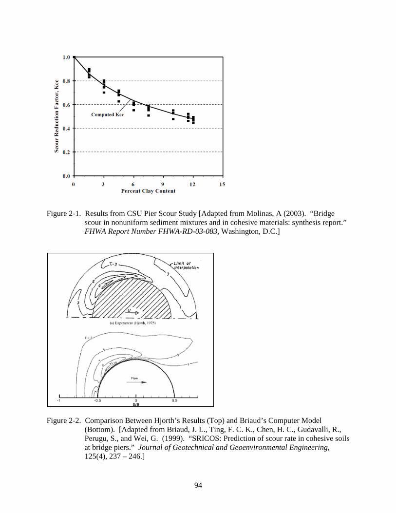
94

Figure 2-1. Results from CSU Pier Scour Study [Adapted from Molinas, A (2003). “Bridge scour in nonuniform sediment mixtures and in cohesive materials: synthesis report.” FHWA Report Number FHWA-RD-03-083, Washington, D.C.]

Figure 2-2. Comparison Between Hjorth’s Results (Top) and Briaud’s Computer Model (Bottom). [Adapted from Briaud, J. L., Ting, F. C. K., Chen, H. C., Gudavalli, R., Perugu, S., and Wei, G. (1999). “SRICOS: Prediction of scour rate in cohesive soils at bridge piers.” Journal of Geotechnical and Geoenvironmental Engineering, 125(4), 237 – 246.]

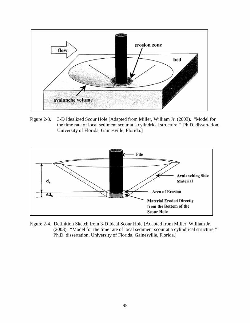
95

Figure 2-3. 3-D Idealized Scour Hole [Adapted from Miller, William Jr. (2003). “Model for the time rate of local sediment scour at a cylindrical structure.” Ph.D. dissertation, University of Florida, Gainesville, Florida.]

Figure 2-4. Definition Sketch from 3-D Ideal Scour Hole [Adapted from Miller, William Jr. (2003). “Model for the time rate of local sediment scour at a cylindrical structure.” Ph.D. dissertation, University of Florida, Gainesville, Florida.]

96

Figure 2-5. Second Definition Sketch from 3-D Ideal Scour Hole [Adapted from Miller, William

Jr. (2003). “Model for the time rate of local sediment scour at a cylindrical structure.” Ph.D. dissertation, University of Florida, Gainesville, Florida.]

Figure 2-6. Top-View of Pile Definition Sketch [Adapted from Miller, William Jr. (2003). “Model for the time rate of local sediment scour at a cylindrical structure.” Ph.D. dissertation, University of Florida, Gainesville, Florida.]

97

Figure 2-7. Effective Shear Stress vs. Scour Hole Depth [Adapted from Miller, William Jr. (2003). “Model for the time rate of local sediment scour at a cylindrical structure.” Ph.D. dissertation, University of Florida, Gainesville, Florida.]

Figure 2-8. Extended Shields Diagram [Adapted from Mehta, A. J. (2007). “An introduction to hydraulics of fine sediment transport.” OCP 6297 class notes draft, University of Florida, Gainesville, Florida.]

98

Figure 2-9. Ariathurai-Partheniades Relationship for Erosion vs. Shear Stress [Adapted from Mehta, A. J. (2007). “An introduction to hydraulics of fine sediment transport.” OCP 6297 class notes draft, University of Florida, Gainesville, Florida.]

Figure 2-10. Results from Modification of Partheniades Equation [Adapted from Van Prooijen, B. C. and Winterwerp, J. C. (2008). “A stochastic formulation for erosion of cohesive sediments.” Journal of Geophysical Research, Draft Copy, December 9, 2008.]

99

Figure 2-11. Definition Sketch for Rock Fracture [Adapted from Henderson, M. R. (1999). “A laboratory method to evaluate the rates of water erosion of natural rock materials.” M.S. Thesis, University of Florida, Gainesville FL.]

Figure 2-12. ERI Definition Sketch [Adapted from Henderson, M. R. (1999). “A laboratory method to evaluate the rates of water erosion of natural rock materials.” M.S. Thesis, University of Florida, Gainesville FL.]

100

Figure 2-13. Relationship between bulk density and critical shear stress [Adapted from Mitchener, H. and Torfs, H. (1996). “Erosion of mud/sand mixtures.” Coastal Engineering, 29, 1 – 25.]

Figure 2-14. Erosion Rate vs. Excess Shear Stress Relationships [Adapted from Mitchener, H. and Torfs, H. (1996). “Erosion of mud/sand mixtures.” Coastal Engineering, 29, 1 – 25.]

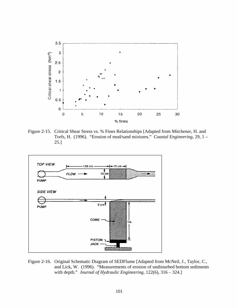
101

Figure 2-15. Critical Shear Stress vs. % Fines Relationships [Adapted from Mitchener, H. and Torfs, H. (1996). “Erosion of mud/sand mixtures.” Coastal Engineering, 29, 1 – 25.]

Figure 2-16. Original Schematic Diagram of SEDFlume [Adapted from McNeil, J., Taylor, C., and Lick, W. (1996). “Measurements of erosion of undisturbed bottom sediments with depth.” Journal of Hydraulic Engineering, 122(6), 316 – 324.]

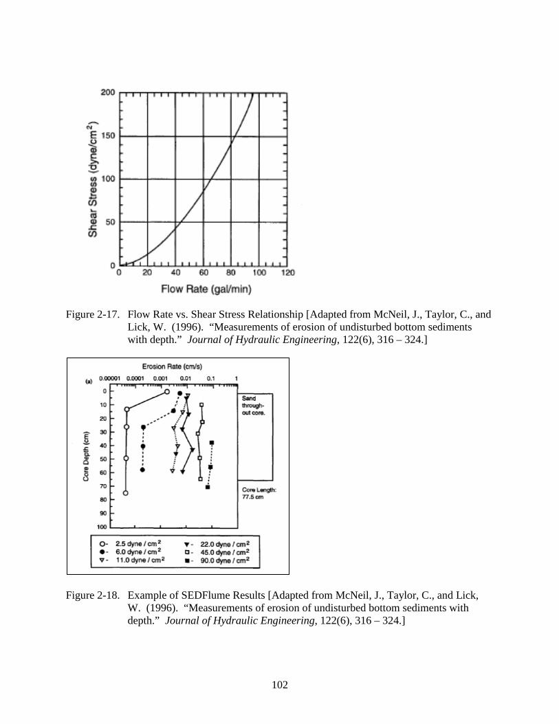
102

Figure 2-17. Flow Rate vs. Shear Stress Relationship [Adapted from McNeil, J., Taylor, C., and Lick, W. (1996). “Measurements of erosion of undisturbed bottom sediments with depth.” Journal of Hydraulic Engineering, 122(6), 316 – 324.]

Figure 2-18. Example of SEDFlume Results [Adapted from McNeil, J., Taylor, C., and Lick, W. (1996). “Measurements of erosion of undisturbed bottom sediments with depth.” Journal of Hydraulic Engineering, 122(6), 316 – 324.]

103

Figure 2-19. Original Schematic of the ASSET [Adapted from Roberts, S. K., and Yaras, M. I. (2006). “Effects of surface roughness geometry on separation-bubble transition.” Journal of Turbomachinery, (128)349, 349 – 356.]

Figure 2-20. Results from ASSET Tests [Adapted from Roberts, S. K., and Yaras, M. I. (2006). “Effects of surface roughness geometry on separation-bubble transition.” Journal of Turbomachinery, (128)349, 349 – 356.]

104

Figure 2-21. Photograph of the EFA [Adapted from Briaud, J. L., Chen, H. C. and Ting, F. (2010). “The, EFA, erosion function apparatus: an overview.” http://tti.tamu.edu/conferences/scour/sample_paper.pdf, March 23, 2010.]

Figure 2-22. Schematic of 1 mm EFA protrusion into flume [Adapted from Briaud, J. L., Chen, H. C. and Ting, F. (2010). “The, EFA, erosion function apparatus: an overview.” http://tti.tamu.edu/conferences/scour/sample_paper.pdf, March 23, 2010.]

105

Figure 2-23. An example of a Moody Diagram [Adapted from Davis, Tom. “Moody Diagram.” Matlab Central, http://www.mathworks.com/matlabcentral/fileexchange/7747-moody-diagram, November 11, 2010.]

Figure 2-24. Photograph of the RETA [Adapted from Sheppard, D. M., Bloomquist, D. and

Slagle, P. M. (2006). “Rate of erosion properties of rock and clay (correlation of erosion rate-shear stress relationships with geotechnical properties of rock and cohesive sediments).” FDOT Report for Project Number BD-545, RPWO #3.]

106

Figure 2-25. RETA Sample Annulus [Adapted from Sheppard, D. M., Bloomquist, D. and


Figure 2-26. RETA Sample Annulus (Close-up) [Adapted from Sheppard, D. M., Bloomquist,

D. and Slagle, P. M. (2006). “Rate of erosion properties of rock and clay (correlation of erosion rate-shear stress relationships with geotechnical properties of rock and cohesive sediments).” FDOT Report for Project Number BD-545, RPWO #3.]

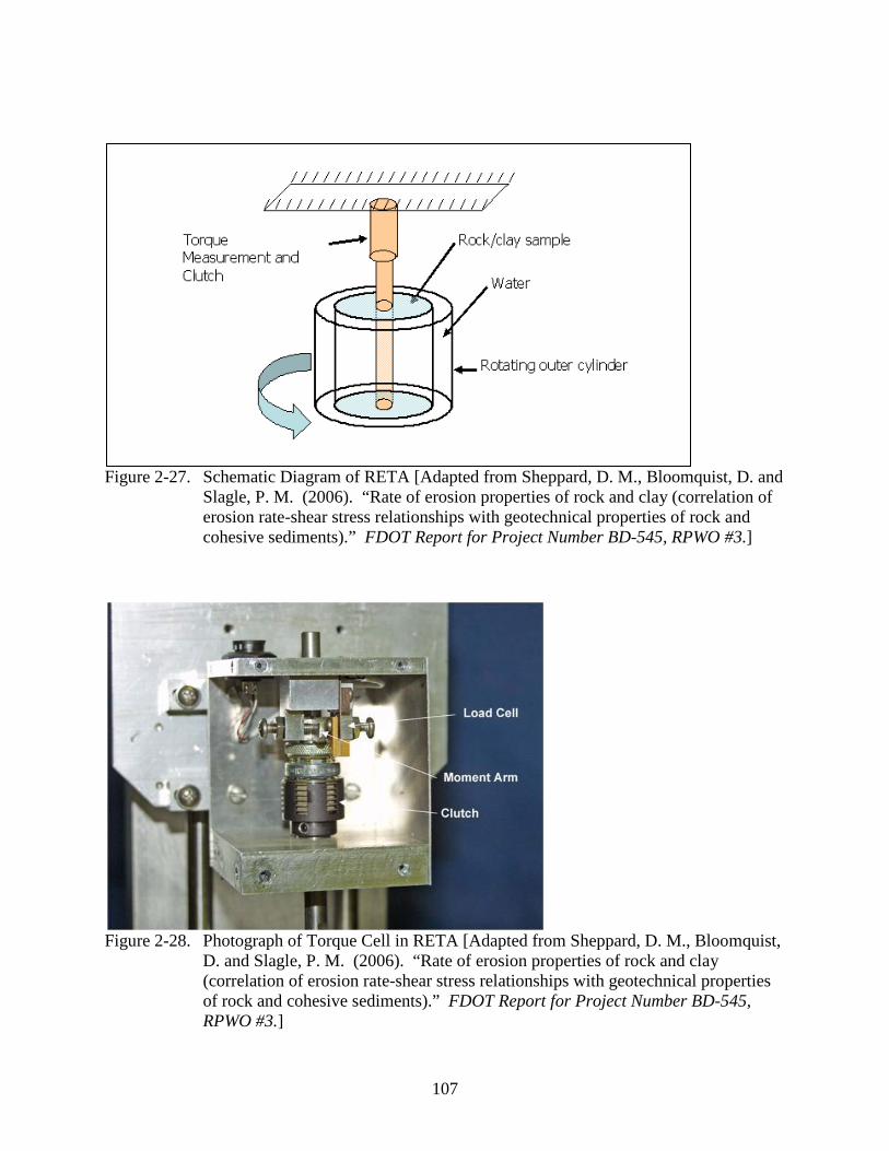
107

Figure 2-27. Schematic Diagram of RETA [Adapted from Sheppard, D. M., Bloomquist, D. and


Figure 2-28. Photograph of Torque Cell in RETA [Adapted from Sheppard, D. M., Bloomquist,

D. and Slagle, P. M. (2006). “Rate of erosion properties of rock and clay (correlation of erosion rate-shear stress relationships with geotechnical properties of rock and cohesive sediments).” FDOT Report for Project Number BD-545, RPWO #3.]

108

Figure 2-29. Photograph of Rock Sample in RETA [Adapted from Sheppard, D. M.,

Bloomquist, D. and Slagle, P. M. (2006). “Rate of erosion properties of rock and clay (correlation of erosion rate-shear stress relationships with geotechnical properties of rock and cohesive sediments).” FDOT Report for Project Number BD-545, RPWO #3.]

Figure 2-30. Top View of RETA [Adapted from Sheppard, D. M., Bloomquist, D. and Slagle,

P. M. (2006). “Rate of erosion properties of rock and clay (correlation of erosion rate-shear stress relationships with geotechnical properties of rock and cohesive sediments).” FDOT Report for Project Number BD-545, RPWO #3.]

109

Figure 2-31. Relationship between shear stress and erosion rate for different Jewfish Creek

Limestone samples [Adapted from Slagle, P. M. (2006). Correlations of erosion rate-shear stress relationships with geotechnical properties of rock and cohesive sediments. M.S. thesis, University of Florida, Gainesville, Florida.]

Figure 2-32. Relationship between cohesion and erosion rate for different shear stresses from

Jewfish Creek Limesonte data set [Adapted from Slagle, P. M. (2006). Correlations of erosion rate-shear stress relationships with geotechnical properties of rock and cohesive sediments. M.S. thesis, University of Florida, Gainesville, Florida.]

Erosion Rate vs Cohesive Strength

0.0

0.1

0.2

0.3

0.4

0.5

0.6

0.7

0 0.5 1 1.5 2 2.5 3 3.5 4MillionsCohesive Strength (Pa)

Eros

ion

Rate

(cm

/yr)

30 Pa35 Pa40 Pa45 Pa50 Pa55 Pa60 Pa65 Pa70 Pa75 Pa80 Pa

110

Figure 2-33. Definition sketch for Cohesion Derivation

Figure 2-34. Typical results from Slagle’s Gator Rock tests. The pink data points are from the

SERF and the blue data points are from the RETA [Adapted from Slagle, P. M. (2006). Correlations of erosion rate-shear stress relationships with geotechnical properties of rock and cohesive sediments. M.S. thesis, University of Florida, Gainesville, Florida.]

τ

σ

111

Figure 2-35. Photograph of the SERF (Side View) [Adapted from Trammel, M. A. (2004).

“Laboratory apparatus and methodology for evaluating water erosion rates of erodible rock and cohesive sediments.” M.S. thesis, University of Florida, Gainesville, Florida.]

Figure 2-36. Top View of the SERF (Original Design) [Adapted from Trammel, M. A. (2004).


112

Figure 2-37. Pumps used to drive water through the SERF [Adapted from Trammel, M. A.

(2004). “Laboratory apparatus and methodology for evaluating water erosion rates of erodible rock and cohesive sediments.” M.S. thesis, University of Florida, Gainesville, Florida.]

Figure 2-38. Eroding Sample Section of the SERF [Adapted from Trammel, M. A. (2004).


113

Figure 2-39. Viewing Window on SERF [Adapted from Trammel, M. A. (2004). “Laboratory apparatus and methodology for evaluating water erosion rates of erodible rock and cohesive sediments.” M.S. thesis, University of Florida, Gainesville, Florida.]

Figure 2-40. Schematic Drawing of Ultrasonic Ranging System [Adapted from Trammel, M. A.


114

Figure 2-41. Top View of Ultrasonic Depth Sensor on SERF [Adapted from Trammel, M. A.


Figure 2-42. Rokni’s Results [Adapted from Rokni, M., Olsson, C., and Sunden, B. (1998). “Numerical and experimental investigation of turbulent flow in a rectangular duct.” International Journal for Numerical Methods in Fluids, 28, 225 – 242.]

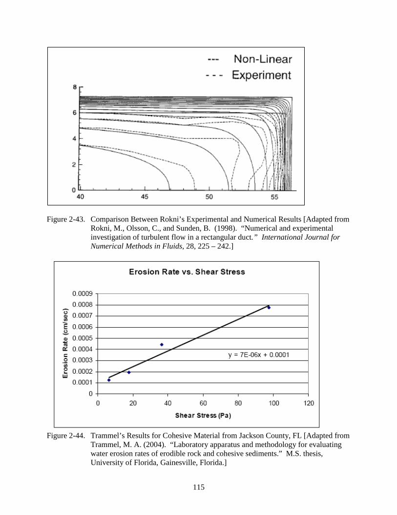
115

Figure 2-43. Comparison Between Rokni’s Experimental and Numerical Results [Adapted from Rokni, M., Olsson, C., and Sunden, B. (1998). “Numerical and experimental investigation of turbulent flow in a rectangular duct.” International Journal for Numerical Methods in Fluids, 28, 225 – 242.]

Figure 2-44. Trammel’s Results for Cohesive Material from Jackson County, FL [Adapted from

Trammel, M. A. (2004). “Laboratory apparatus and methodology for evaluating water erosion rates of erodible rock and cohesive sediments.” M.S. thesis, University of Florida, Gainesville, Florida.]

116

Figure 2-45. Graph of Typical Temperature Rise During Longer SERF Tests

Figure 2-46. Eroded Gator Rock 2.0 Sample.

117

CHAPTER 3 ENHANCEMENTS AND IMPROVMENTS TO THE SEDIMENT EROSION RATE FLUME

3.1 Introduction

As discussed in Chapter 2, when originally built, the Sediment Erosion Rate Flume (SERF)

was designed to be one of the most advanced erosion rate-testing devices in the world. Still, the

issues with the device outlined in Chapter 2, prevented the device from being as accurate as one

might need when developing shear stress-erosion rate relationships for use in the Sheppard-

Miller method or the EFA-SRICOS method. The specific issues with the flume have already

been described in detail, but to summarize, testing was limited because of the following factors:

1. When cohesive sediments were used, the ultrasonic pulses from the ultrasonic ranging system (SEATEK) often penetrated into the samples.

2. Water temperature in the flume increased over longer-durations tests.

3. Shear stress was not measured directly; rather it was inferred via a pressure drop.

In addition to fixing these issues with the SERF, another goal of this study was to make the

flume operable for two more sets of experimental conditions:

1. The first goal was to strictly control recirculating sediment as it passes through the flume so that clear water vs. live bed conditions could be more precisely regulated and isolated from one another.

2. The second goal was to study the effects of upstream artificially induced vortices on both shear stress and erosion rate development.

This chapter discusses the improvements, enhancements, and additions made to the SERF

to solve the original issues associated with testing and meet the new experimental goals for this

project.

3.2 Laser Leveling System

The ultra-sonic pulse sample penetration problem was introduced in Chapter 2. To combat

this issue, in the past, researchers like Slagle, who was actually the only previous researcher to

use cohesive sediment in the SERF, only had one option – to input an artificial depth value in the

118

motor feedback loop program. The depth from the top of the flume to the top of the sample

should be 4.92 cm. When Slagle tested cohesive material with the SEATEK (ultra-sonic ranging

system) and the SEATEK returned depth values that deviated from the correct 4.92 cm reading,

his solution was to tell the computer to use a different comparative depth. So, for example if on

average the sand-clay mixture was returning a level value of 5.20 cm, this was used as the basis

for comparison.

There were a several issues associated with this procedure. If Slagle was going to use the

user-defined input parameter to level his samples, he would have standardized his testing

procedure. Slagle’s recommendation when experimenting on a sample that is experiencing

ultrasonic penetration is essentially to run the SEATEK while the flume is running, and observe

what the SEATEK return values should have been. A better method would have been to run the

SEATEK for a specified time length while the sample was level with the flume bottom and pump

speed was low (to prevent erosion). Then, SEATEK data would be recorded, an average would

be taken, and this quantity would be used as the user-defined input value. Slagle does not

explain why he did not use this method, but further analysis shows that even doing this would

have not worked.

Experience with the SERF shows that at higher flow rates, return pulse timing yields a

greater depth than it would have yielded at a slower flow rate. At first, this result appeared

puzzling since the SEATEK should work independently from flow speed. This is because at

higher flow rates, erosion rates are higher as well. Although a filter was added to the device (to

be discussed in Section 3.5), the filter was unable to keep up with rapid cohesive erosion. The

filter was also incapable of removing fine material from suspension such that when clayey

samples eroded, there was often tiny clay flocs present in the water column.

119

When the ultrasonic pulses hit a sample (and potentially penetrate it), the presumption is

that they are traveling in a straight line. As the pulses get deflected or diffracted, the time that it

takes the pulses to return to their source increases. When more material is in suspension, as it is

at higher flow rates because of recirculating material, the pulses will get deflected or diffracted

more frequently. This causes a slightly slower pulse return time, which in turn translates into an

apparent deeper SEATEK reading. Combine this with penetration effects, and it’s obvious that a

user-defined solution cannot work. To set up this condition quantitatively, one would have to

run the SERF at a certain flow speed and continuously manually level off the sample with the

flume bottom. Then, the SEATEK return values would be recorded, averaged, and the correct

user-defined depth would be known. Lastly, the test could be repeated such that the feedback

mechanism, not user control, would govern sample advancement.

With this procedure, one of the SERF’s advantages is eliminated because development of

the flow speed vs. user-defined depth correlations would be dependent on operator input. Under

these conditions then, the SERF would in effect be the same as the EFA, the ASSET, or the

SEDFlume. Secondly, this procedure would double the amount of time it takes to obtain a

dataset. The manual advancement step in the previous procedure would have produced its own

erosion rate shear stress curve.

It is also likely that for a given flow speed, user-defined depth would have changed

dynamically with time. In other words, as a sample erodes, more of the eroded portion of the

sample recirculates back through the SERF. As this occurs, sediment concentration in the water

column increases, which in turn causes a greater scatter frequency over the course of the test. In

other words, if at the beginning of the test the SEATEK output a depth of 5.10 cm, by the end of

120

the test due to the increase in particle concentration, the SEATEK would output a higher depth

such as 5.30 cm.

Even if this could be accounted for, this ignores the fact that different sand-clay

compositions yield different penetration depths. For example, penetration into a 25% sand

sample is different from penetration into a 75% sample. To calibrate this procedure would

require the development of an increasingly complicated set of curves and correction factors, and

even with this, would likely not work as expected.

One goal of this project was to make the SERF capable of testing sand-clay materials.

Because the SEATEK cannot be used as a stand-alone system when cohesive sediment is used,

something else needed to be invented and installed. There are two ways to measure whether or

not a sample is level with the flume bottom. The SEATEK approach involves a top-down design

where measurements from a fixed point above the sample determine whether or not the sample

needs to be advanced. The second approach – a flushness approach – had not yet been tried.

The simple analogy to a flushness approach is the safety for a garage door opener. The

safety is designed such that at one end of the garage door, a laser is aimed at a corresponding

photoelectric sensor at the other side of the door. If the photoelectric sensor can see the laser, it

must mean that the path for the garage door is clear, and the door is allowed to operate. If the

sensor cannot see the laser, then something is blocking the laser’s path. Under these conditions,

a voltage is sent back through a feedback loop with the garage door opener’s motor, and the

motor is not allowed to operate until this voltage switch is on – or until the laser is no longer

blocked.

A similar design to this was installed in the SERF. Using miniature fiber-optics, a series of

three lasers and three corresponding photoelectric sensors were installed along the top of the

121

flume’s bottom wall (Figure 3-1). Diameter of the lasers and photoelectric sensors were 1.50

mm. Signals from the photoelectric sensors are amplified so that a light signal can be read even

when the flume is full of water (Figure 3-2). Output from the amplifiers is sent through a control

box, into the computer’s SCC-2345 analog signal processor, to the computer’s PCI-6310 card,

and to the Labview control program.

Using the same principles as a garage door opener, if a laser-photoelectric sensor pair is

blocked, it must be blocked by the sample. Under these conditions then, the motor will not

move. When the laser-photoelectric sensor pair becomes uncovered, it must mean that the

sample needs to be advanced. Qualitative testing with the laser-photoelectric sensor pairs before

SERF installation showed two things:

1. This system would work under cloudy water conditions that would be seen during sand-clay erosion testing.

2. This system would be able to provide a recess resolution of approximately half the laser diameter – or approximately 0.75 mm.

The second point is discussed in some detail. When the lasers are operating, the motor will

not move until all of them (if AND logic is used) or some of them (if OR logic is used) are

uncovered. Only when the correct combination of lasers is uncovered will a sample advance.

The advancement minimum then – 0.75 mm – becomes the associated error with this design. In

other words, when the lasers are engaged, the sample cannot advance unless at least 0.75 mm of

material has eroded from it. The SEATEK was slightly more precise as it would cause

advancement/retraction with a depth deviation of 0.5 mm. This design error is of the same order

of magnitude as the SEATEK, and smaller waterproof lasers could not be found.

Although three lasers were used during this study due to budget limitations, it is easy to see

how to idealize this design. Often, samples in the SERF erode non-uniformly. For example,

certain sand clay mixtures exhibit erosion characteristics where their front face erodes much

122

slower than their back edge. Rather than using three lasers spaced at a certain interval, the most

effective design for a laser leveling system would be to install a continuous laser array and

corresponding photoelectric sensors. This would eliminate the AND logic vs. OR logic question

and instead allow a certain percentage of eroding sample length to determine sample

advancement. Implementation of this complete system would not have fit within this project’s

budget constraints however, and therefore was economically not feasible. When implemented,

the laser system as installed worked as it was designed. Due to differential erosion rates, the

lasers were programmed such that OR logic was used. Therefore, if two of the three lasers

became uncovered, the sample advanced.

Although the primary purpose of the laser leveling system was to allow for cohesive

sediment testing, another valuable aspect of the system is that when non-cohesive sediments are

used in the SERF, it can be used as a redundant check in conjunction with the SEATEK.

Although not as common as with cohesive sediments, when sands are tested at high flow rates,

sometimes sand particles can be seen recirculating back through the flume. As with clays,

recirculation causes SEATEK errors, but with the implementation of the lasers, these errors can

be reduced. During non-cohesive testing then, instead of using the SEATEK or the lasers as

independent systems, the following feedback algorithm was programmed:

1. Check to see if the middle laser and either the front or back laser is uncovered.

2. Read depth from SEATEK.

3. If the correct laser sequence is uncovered and the SEATEK says that top-depth is greater than 0.5 mm, record the SEATEK depth deviation.

4. Move sample required amount.

5. Go back to (1)

123

This laser leveling system is the only known system like it in an erosion rate testing device,

it has helped to reduce the number of SEATEK errors when non-cohesive sediments are present,

and it has allowed the SERF to be used for testing cohesive materials. The introduction of the

laser leveling system is the most significant upgrade made to the SERF during this project.

3.3 Temperature Control System and Temperature Patch for SEATEK

Besides the SERF’s initial inability to test cohesive materials, the next issue with the

device was the temperature rise during longer tests discussed in Chapter 2. Because of the speed

of sound’s dependence on water temperature, the temperature rise caused the SEATEK to

malfunction and could have caused damage to the SEATEK. The SEATEK gets hot as it sends

ultrasonic pulses and it is dependent on a steady stream of water to cool itself. If the water gets

too hot, the SEATEK will be damaged. Also, a temperature rise during tests is not typical in

nature and should be avoided.

To combat against temperature rises during tests, a temperature control device was

installed. There were several designs that were considered when designing the temperature

controlling apparatus. For example, there is a chilled water line that runs through Reed Lab

(where the SERF was built), and there was talk at one point about running a cooling coils of that

line into the reservoir tank. This design was ultimately rejected because there was a less

expensive, more efficient option.

Eventually, the final cooling method was developed using a water chiller. There were two

options for water chiller design. The first option involved sending flow through the SERF (2,000

gpm during max capacity) through the chiller so that it could be cooled. However, a chiller with

2,000 gpm capacity is prohibitively expensive, and it was not feasible with the budget constraints

of the project.

124

The second chiller option was to install a cooling device in parallel with the SERF pumps.

Although the temperature rise in the SERF is large over a 24-hour time scale, over a one-hour

time span it is actually relatively small. Temperature only rises approximately 2oC per hour

during maximum capacity flow conditions. Because of this, it was possible to design a chiller

that was just large enough to keep up with that degree of temperature rise at a much lower flow

rate. A 6-ton chiller was installed in parallel with the primary pumps and powered by an internal

30-hp pump (Figure 3-3). The RTS-603 Rite Temp Water Chiller runs at a flow rate of

approximately 30 gpm, and it is capable of removing 72,000 BTU/hr. of heat. Because the

temperature in the SERF reservoir tank rose at approximately 2oC/hr., the following calculation

was conducted to make sure that the 6-ton chiller could keep up with the temperature rise:

d.req' BTU/hr. ,00005~ rise) (temp 3.6* (S.F.) 1.5*9,177 gal 1

ft 1337.0*ft

lb 62.4*gal 1100 o3

F=

As shown here, the 6-ton chiller is oversized by approximately 30% even with a safety

factor of 2.0 built into the calculation. Although a 5-ton chiller could have done the job (max

capacity of 60,000 BTU/hr.) the chiller was oversized for two reasons. First, the 6-ton chiller

wasn’t much more expensive than the 5-ton chiller. Secondly, the 6-ton chiller is capable of

cooling water in the tank more quickly. This means that the 6-ton chiller’s compressor will shut

off more often and it will not have to run constantly. Because the chiller is not continually

running, it will save electricity and it will lessen the chance that the chiller could break.

To confirm that the chiller was the proper size, a cooling test was conducted in the SERF

reservoir tank (Figure 3-4). As demonstrated, the chiller is capable of producing a temperature

drop of approximately 3.0oC/hr. and temperature in the tank appears to respond to the

relationship given by Equation 3-1:

125

if TtT +−= 05.0 (3-1)

where t is the time in minutes and Ti is the initial temperature.

Once the water chiller had been installed, the SERF was capable of running longer-

duration tests. This was essential for testing of rock-like materials because these tests often take

24-hours or more.

Once the temperature had been regulated, the SEATEK feedback loop was studied one

more time. In the past, getting the SEATEK up and running was cumbersome from a computing

standpoint. Previously, SERF users were required to open a serial connection with

HyperTerminal or TeraTermainal, input a water temperature, and start a data run. Then, the

experimenter would close HyperTerminal, start the control program that was written in Labview,

and every time the Labview program ran through another loop, it would read output data from

the SEATEK on the serial port.

The obvious problem with this method is that water temperature is only being fed to the

SEATEK once at the beginning of the test. The temperature control system can effectively

regulate temperature to +/-2oC, yet even within this range, the SEATEK is supposed to be

accurate within 0.5 mm. Because the speed of sound in water is so dependent on water

temperature, if the SEATEK does not know the exact water temperature precisely, it will output

a depth value that is incorrect.

A thermocouple had been installed in the SERF, but had not been incorporated into a

feedback loop with the SEATEK. The presence of the thermocouple makes it possible to

program the actual temperature to the SEATEK in real-time. A patch was written in Labview for

the control program so that before the SEATEK takes a depth reading, it first is given a

temperature reading from the thermocouple so that it knows what the correct ultrasonic pulse

126

return time should be at that temperature. Although a quantitative analysis of error reduction

was not conducted after installation of this temperature patch, qualitatively it appears that when

the SEATEK is used as a stand-alone system now, particularly at low flow speeds, the sample

appears to say more level with the flume’s bottom. SERF computer programs including the new

control system with the temperature patch are presented in Appendix C.

3.4 New Shear Stress System

As discussed in Chapter 2, other flume-style erosion-rate testing devices such as the EFA,

the ASSET, the SEDFlume, and the original SERF did not measure shear stress on an eroding

sample directly. Rather, shear stress was inferred in a few different ways. The EFA inferred

shear stress from a Moody diagram; the ASSET and the SEDFlume inferred shear stress from a

relationship obtained from the Darcy-Weisbach equation; and the SERF used a pressure drop

relationship to infer shear stress.

When these other flumes were developed, the technology did not exist to measure shear

stress directly. While some of these approximating methods are accurate, and some of them are

not, there was no way to quantify which were better than the others. To definitively answer how

to properly measure shear stress in a flume-style erosion rate testing device, three sets of

improvements were made to the SERF.

3.4.1 Shear Stress Sensor

The issue with measuring shear stress in devices like the SERF in the past stemmed from

the inability to accurately measure shear stresses of small magnitudes. In the SERF, at high flow

rates, a relatively high the shear stress is 100 Pa (0.015 psi) while typically at lower flow rates

shear stresses are around 10 Pa (0.0015 psi). These stress values are much too small to be picked

up accurately by most commercial strain gauges or pressure sensors.

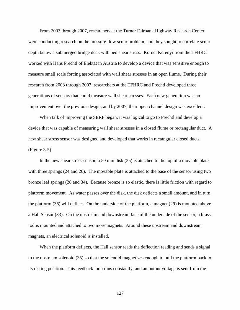
127

From 2003 through 2007, researchers at the Turner Fairbank Highway Research Center

were conducting research on the pressure flow scour problem, and they sought to correlate scour

depth below a submerged bridge deck with bed shear stress. Kornel Kerenyi from the TFHRC

worked with Hans Prechtl of Elektat in Austria to develop a device that was sensitive enough to

measure small scale forcing associated with wall shear stresses in an open flume. During their

research from 2003 through 2007, researchers at the TFHRC and Prechtl developed three

generations of sensors that could measure wall shear stresses. Each new generation was an

improvement over the previous design, and by 2007, their open channel design was excellent.

When talk of improving the SERF began, it was logical to go to Prechtl and develop a

device that was capable of measuring wall shear stresses in a closed flume or rectangular duct. A

new shear stress sensor was designed and developed that works in rectangular closed ducts

(Figure 3-5).

In the new shear stress sensor, a 50 mm disk (25) is attached to the top of a movable plate

with three springs (24 and 26). The movable plate is attached to the base of the sensor using two

bronze leaf springs (28 and 34). Because bronze is so elastic, there is little friction with regard to

platform movement. As water passes over the disk, the disk deflects a small amount, and in turn,

the platform (36) will deflect. On the underside of the platform, a magnet (29) is mounted above

a Hall Sensor (33). On the upstream and downstream face of the underside of the sensor, a brass

rod is mounted and attached to two more magnets. Around these upstream and downstream

magnets, an electrical solenoid is installed.

When the platform deflects, the Hall sensor reads the deflection reading and sends a signal

to the upstream solenoid (35) so that the solenoid magnetizes enough to pull the platform back to

its resting position. This feedback loop runs constantly, and an output voltage is sent from the

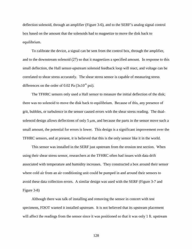
128

deflection solenoid, through an amplifier (Figure 3-6), and to the SERF’s analog signal control

box based on the amount that the solenoids had to magnetize to move the disk back to

equilibrium.

To calibrate the device, a signal can be sent from the control box, through the amplifier,

and to the downstream solenoid (27) so that it magnetizes a specified amount. In response to this

small deflection, the Hall sensor-upstream solenoid feedback loop will react, and voltage can be

correlated to shear stress accurately. The shear stress sensor is capable of measuring stress

differences on the order of 0.02 Pa (3x10-6 psi).

The TFHRC sensors only used a Hall sensor to measure the initial deflection of the disk;

there was no solenoid to move the disk back to equilibrium. Because of this, any presence of

grit, bubbles, or turbulence in the sensor caused errors with the shear stress reading. The dual-

solenoid design allows deflections of only 5 µm, and because the parts in the sensor move such a

small amount, the potential for errors is lower. This design is a significant improvement over the

TFHRC sensors, and at present, it is believed that this is the only sensor like it in the world.

This sensor was installed in the SERF just upstream from the erosion test section. When

using their shear stress sensor, researchers at the TFHRC often had issues with data drift

associated with temperature and humidity increases. They constructed a box around their sensor

where cold air from an air conditioning unit could be pumped in and around their sensors to

avoid these data collection errors. A similar design was used with the SERF (Figure 3-7 and

Figure 3-8)

Although there was talk of installing and removing the sensor in concert with test

specimens, FDOT wanted it installed upstream. It is not believed that its upstream placement

will affect the readings from the sensor since it was positioned so that it was only 1 ft. upstream

129

from the test section. However, until velocity profiles can accurately be measured in the SERF,

there is no way to be sure of this.

3.3.2 New Pressure Transducers

The second shear stress system enhancement that was made to the SERF was the

installation of a set of new pressure transducers. When the flume was originally designed

(Trammel 2004), pressure difference upstream and downstream from the sample was measured

with a transducer with a range of +/- 2.5psi (14,000 Pa). The accuracy of this device was 0.02%

times its range which equals 5.2 Pa. When one examines the formula for converting pressure

difference along a flume’s walls to shear stress:

( )Lwlplw22 +

∆=τ

(3-2)

and uses an order of magnitude argument, it becomes obvious that measuring a pressure

differential with 5.2 Pa accuracy could be better. In this equation, l = 4.44 cm, w = 20.32 cm,

and L = 10.16 m. Substituting into equation 3.3-1, τ is accurate to +/-0.50 Pa, which is well

below the accuracy of the shear stress sensor.

In 2006, Slagle tried to improve the accuracy of the device by installing a differential

pressure transducer that had a range of +/-10 inches of water (+/- 2450 Pa). This improved the

accuracy of shear stress estimations from the pressure drop to +/-0.0891 Pa. Although Slagle’s

improvement gave more accurate shear stress data, the drawback was that the new sensors were

ultrasensitive to over pressurizing and they often broke due to operational error. Often, a hose

would be connected that was too long, and as a result, the membrane inside the sensor would

snap or “pop” causing the sensor to break. This mistake happened often, and every time it

happened, a new sensor would need to be purchased.

130

Slagle had the right idea when improving the accuracy of his pressure sensors, he chose

sensors from Sensotec that had little over pressurization tolerance. During this project, the most

effective aspects from Slagle and Trammel’s design were combined. A new sensor system was

purchased from Omega Engineering, and these sensors were capable of withstanding over

pressurization forces of approximately 50 psi., while their range was accurate to +/-0.02% of 0.5

psi (3447 Pa). Although slightly less accurate than Slagle’s sensor, they do not break as often,

and they are close to the accuracy of Slagle’s. Two sensors and four pressure ports were

installed in the SERF (Figure 3-9).

The first set of taps was installed upstream and downstream from the sample section while

the second set of taps were positioned upstream and downstream from the shear stress sensor.

The motivation behind this setup originally was to use the sensors as a “check” of the shear

stress sensor, but as Chapter 4 will discuss, this may not be the most effective solution because

inferring shear stress from a pressure drop may not be correct.

3.4.3 Paddlewheel Flow meter

The third shear stress system improvement that was made was the installation of a

paddlewheel flow meter. In 2004, Trammel measured SERF velocity using an ultrasonic

velocity flow meter (Figure 3-10), but ultrasonic flow meters are not accurate enough.

Trammel’s velocity correlation appeared incorrect physically – it was logarithmically distributed

which implies that for a low pump frequency, a negative velocity should ensue – so operators

knew that it was questionable. To properly evaluate the Briaud Moody Diagram method and the

Flat Wall method for estimating shear stress, an accurate velocity vs. pump speed distribution

was required. When the first round of tests were conducted, investigators tried to use Trammel’s

velocity correlation in the Colebrook Equation (which describes the Moody Diagram to be

discussed in Chapter 4) and Flat Wall equations, but results were such were even under flat

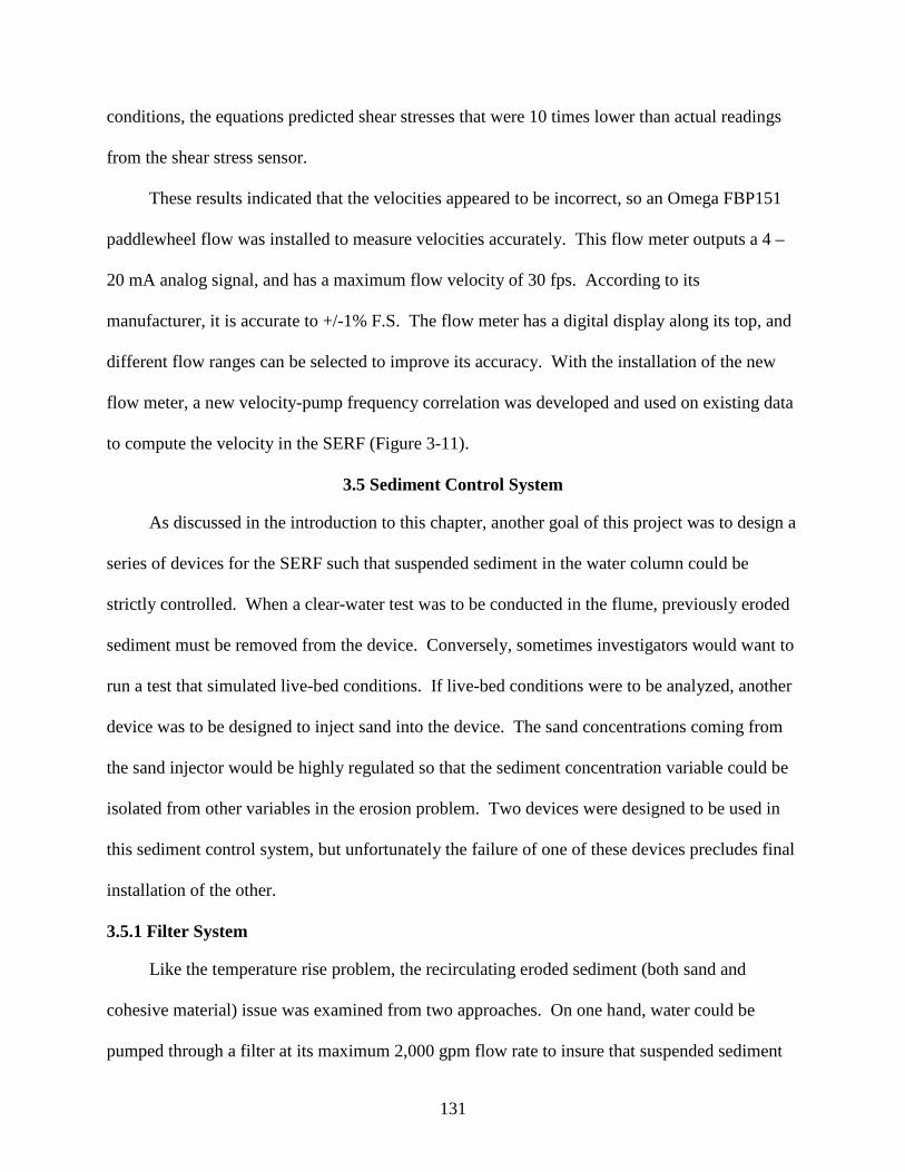
131

conditions, the equations predicted shear stresses that were 10 times lower than actual readings

from the shear stress sensor.

These results indicated that the velocities appeared to be incorrect, so an Omega FBP151

paddlewheel flow was installed to measure velocities accurately. This flow meter outputs a 4 –

20 mA analog signal, and has a maximum flow velocity of 30 fps. According to its

manufacturer, it is accurate to +/-1% F.S. The flow meter has a digital display along its top, and

different flow ranges can be selected to improve its accuracy. With the installation of the new

flow meter, a new velocity-pump frequency correlation was developed and used on existing data

to compute the velocity in the SERF (Figure 3-11).

3.5 Sediment Control System

As discussed in the introduction to this chapter, another goal of this project was to design a

series of devices for the SERF such that suspended sediment in the water column could be

strictly controlled. When a clear-water test was to be conducted in the flume, previously eroded

sediment must be removed from the device. Conversely, sometimes investigators would want to

run a test that simulated live-bed conditions. If live-bed conditions were to be analyzed, another

device was to be designed to inject sand into the device. The sand concentrations coming from

the sand injector would be highly regulated so that the sediment concentration variable could be

isolated from other variables in the erosion problem. Two devices were designed to be used in

this sediment control system, but unfortunately the failure of one of these devices precludes final

installation of the other.

3.5.1 Filter System

Like the temperature rise problem, the recirculating eroded sediment (both sand and

cohesive material) issue was examined from two approaches. On one hand, water could be

pumped through a filter at its maximum 2,000 gpm flow rate to insure that suspended sediment

132

was removed from it. On the other hand, an independent filtering mechanism could be installed

in series with the water chiller to act as a secondary system – similar to the way in which a

swimming pool or a hot tub works.

Because of budget constraints, the second option was chosen. While the independent

system design worked well with the water chiller, it did not work well with the filter. During a

day of testing, particularly with sand-clay mixtures, visual observation showed that as testing

continued, water became cloudier. Although quantitative measurements of sediment

concentration were not conducted, qualitatively, by the end of a full day of testing, the camera

could not see the eroding sample from its viewing port. This means that there was less than 10

cm of visibility in the flume.

At first, it was assumed that this cloudiness was the result of suspended clay flocs in the

water column. Eventually, after a day of testing the flume was emptied as it was after every day

of testing, and as water exited the flume 5-gallon bucket samples of water were taken. Material

was allowed to settle out of suspension, and as the eroded material settled, the resulting residue

showed that sand and clay had stuck together to form sand-clay flocs. These sand-clay flocs

were suspended in the water column during testing, and they were the causing some of the

cloudiness in the water column.

This is not to say that the filter did nothing to help. After each round of testing, the

reservoir tank was emptied, refilled with clean water, the filter was backwashed, and then the

tank was filled again. Backwashing the filter revealed even cloudier (qualitatively) water than

the dirty water that drained from the tank after a day of testing. It appears that the filter was

doing some work in terms of removing suspended sediment from the water column, but after a

day of extensive SERF testing (approximately 4 samples were tested per day), the filter simply

133

could not keep up with the sediment influx rate. Whereas the smaller water chiller could keep up

with a 2oC temperature rise, the filter could not keep up with particle concentrations rising to

0.50g/L over the course of 5 hours of testing ([~500 g of solid material per sample*4 tests per

day ] divided by1,100 gallons[ 4,164 L] = 0.48 g/L). Or, put another way, the sand filter could

not keep up with sediment concentration increases of 0.1 g/L per hr.

The pump that drives the filter runs at approximately 30 gpm. Therefore, assuming

uniform mixing, it would take the filter approximately 37minutes to filter the water in the

reservoir tank. If this were the case, then breaks between tests to change the sample, reset the

computer program, analyze data, etc. should have given the filter enough time to clean the tank’s

water. Because visually it was not happening, either:

1. The filter cannot filter fine enough particles out of the water. 2. Water in the reservoir tank is not being uniformly mixed.

It is difficult to isolate which of these two possibilities presented the largest problem with

filtration, although because the installed filter was a sand filter, it is likely that it was unable to

remove the small diameter particles from suspension. Still, even if a finer filter was used, it is

unclear whether or not it would have any effect as much of the particulate that drained from the

reservoir tank after testing was sandy.

Because of the filter’s failure during sand-clay tests, results from the latest round of sand-

clay tests in the SERF may be subject to the same criticism as results from the CSU tests. This

was a disappointing development during testing, and it was not anticipated when the filter was

installed.

The second issue that is caused by the sand filter’s failure is that the highly regulated sand

injection system could not be installed in the SERF. Adding another source of sand to the device

without proper filtering would allow even more sediment to cycle back through the flume. Even

134

without the introduction of another sediment source, it is impossible to say how sediment

concentration is changing with time. Within the context of a flume run, suspended sediment

concentration is continually changing. Adding another source of sediment would further skew

the results and not produce valid data because it would be impossible to isolate sand

concentration as a variable.

The third concern from the filter system’s failure is that if the SERF is allowed to run with

high sediment concentrations in the water, the pumps will eventually be compromised. The

centrifugal pumps require a clean water source. If sand is moving through them at high flow

speeds, the net effect is that the pumps’ impellers are, in effect, being sand-blasted. Introduction

of a sand injector would only serve to exacerbate the issue.

Although the SERF has been operable since Trammel started his work in 2002, this latest

round of tests is the only time when the device was used extensively under high erosion

conditions. Analysis of Slagle’s work shows that his data points with the SERF are limited.

Most of Slagle’s work involved RETA testing. When Slagle did use the SERF, erosion rates

were low and the device could not be used for long periods of time (because of the temperature

rise). Therefore, during Slagle’s tenure at UF, the SERF frequently sat idle. Even with this

down-time, when this project began, one of the flume’s primary pumps was already damaged –

presumably because of recirculating sediment. Fortunately this damage was only to the pump’s

seal, and repair was relatively inexpensive. If an impeller had to be replaced though, the cost

could be prohibitively expensive and shut the SERF down for the foreseeable future.

Because of this, a decision was made to limit the dataset as much as possible. The

necessity to do this though was disappointing and unexpected both because it precluded the

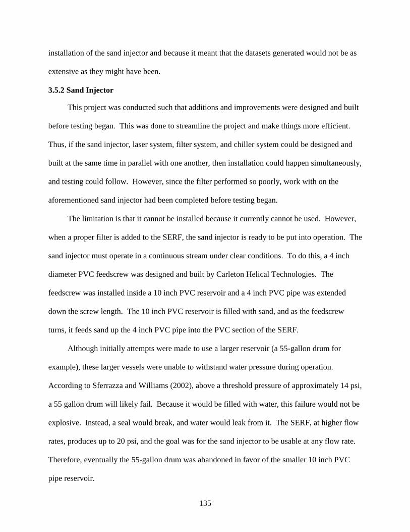
135

installation of the sand injector and because it meant that the datasets generated would not be as

extensive as they might have been.

3.5.2 Sand Injector

This project was conducted such that additions and improvements were designed and built

before testing began. This was done to streamline the project and make things more efficient.

Thus, if the sand injector, laser system, filter system, and chiller system could be designed and

built at the same time in parallel with one another, then installation could happen simultaneously,

and testing could follow. However, since the filter performed so poorly, work with on the

aforementioned sand injector had been completed before testing began.

The limitation is that it cannot be installed because it currently cannot be used. However,

when a proper filter is added to the SERF, the sand injector is ready to be put into operation. The

sand injector must operate in a continuous stream under clear conditions. To do this, a 4 inch

diameter PVC feedscrew was designed and built by Carleton Helical Technologies. The

feedscrew was installed inside a 10 inch PVC reservoir and a 4 inch PVC pipe was extended

down the screw length. The 10 inch PVC reservoir is filled with sand, and as the feedscrew

turns, it feeds sand up the 4 inch PVC pipe into the PVC section of the SERF.

Although initially attempts were made to use a larger reservoir (a 55-gallon drum for

example), these larger vessels were unable to withstand water pressure during operation.

According to Sferrazza and Williams (2002), above a threshold pressure of approximately 14 psi,

a 55 gallon drum will likely fail. Because it would be filled with water, this failure would not be

explosive. Instead, a seal would break, and water would leak from it. The SERF, at higher flow

rates, produces up to 20 psi, and the goal was for the sand injector to be usable at any flow rate.

Therefore, eventually the 55-gallon drum was abandoned in favor of the smaller 10 inch PVC

pipe reservoir.

136

The sand injector’s feedscrew is connected to a variable speed motor control. Although

the motor control is not currently hooked up to the SERF control computer (this step was skipped

since the sand injector was not installed), in the future this upgrade should be made so that the

motor can be computerized.

To regulate sand entering the SERF, the sand injector rests on four, 250-lb capacity load

cells (Figure 3-12). Before a test is conducted, the weight of the sand injector will be known.

During testing, the sand injector weight will decrease, and after testing, the final weight will be

known. By measuring the amount of mass lost, researchers will precisely know the quantity of

sand that was injected.

Because the load cells need to slightly deflect so that they can output a weight signal, two

expansion joints were installed at either end of the sand injector (Figure 3-13). These expansion

joints allow for 0.5 in of deflection, which is less than the deflection of the load cell mounts. A

photograph of the completed sand injector is presented in Figure 3-14. Because the sand injector

was not installed, it could not be calibrated. However when a proper filter is added to the SERF,

it can be easily installed and calibrated.

3.6 Vortex System

Besides sediment control, there was another new scenario under which the SERF was to be

run – the scenario where vortices are generated in the flume upstream from the eroding sample or

shear stress sensor. These vortices do not mimic the horseshoe vortex. The vortex generator is

instead designed such that the presence of an upstream obstruction generates a turbulent wake

region (or vortex region) behind the obstruction. This newly formed turbulent flow regime may

affect erosion rate.

To create this vortex obstruction, a circular cylinder was selected because flow past

circular cylinders has been studied extensively, and flow patterns in the cylinder’s wake region

137

are fairly well understood. From experience at the TFHRC, in flume tests, blockage should less

than 20% of the flume’s cross-sectional area (Crowley 2007). Because the goal was to generate

the largest wake region possible, the maximum cylinder size was chosen. The SERF height is

1.75 in., so the maximum horizontal cylinder that could be used was approximately 3/8 inch to

ensure that blockage requirements were met.

To design the height of the cylinder properly so that full in-tact vortices were produced,

research was conducted on flow fields around circular cylinders near a wall. Because the

eroding test section is loaded into the flume from the bottom, the goal was to generate vortices as

close to the bed as possible. According to Sumer and Fredsoe (2006), when a cylinder is placed

near a wall, the flow around the cylinder changes compared to how it would look if the wall was

not present (Figure 3-15). Among the changes to the flow patterns around a cylinder, the most

important for the SERF is that vortex shedding becomes suppressed for gap ratio values smaller

than approximately e/D = 0.3, where e is the gap between the bottom of the cylinder and the wall

and D is the cylinder’s diameter.

Because the diameter of the cylinder is fixed at 0.375 inches due to blockage requirements,

the minimum gap that could be used to achieve a gap ratio of 0.3 is 0.104 inches. Because this is

a non-standard size and because generally speaking, a larger gap means a larger wake region,

this value was slightly expanded so that the design gap for the vortex generator would be 0.125

inches. This results in a gap ratio of 0.33 which is acceptable.

Once the cylinder and the gap had been properly sized, the Strouhal Number was used to

predict the number of vortex oscillations that will occur. Past tests in the SERF have shown that

erosion does not occur below a Reynolds Number of ~3x102, and based on a 2,000 gpm max

volumetric flow rate limit, the largest Reynolds Number that will ever be present in the SERF is

138

~4.5x104. Within these ranges, the Strouhal number (Equation 3-3 and Figure 3-16) should stay

fixed at approximately 0.2.

U

DfSt v= (3-3)

In Equation 3-3, fv is the vortex shedding frequency, D is the cylinder’s diameter, and U is the

water velocity. Therefore, at low flow rates, vortices should be produced at approximately 0.7

Hz, at high flow rates, approximately 70 Hz, and in between this upper and lower limit, a

Strouhal analysis can be conducted to predict the vortex shedding frequencies at each velocity.

Analysis was conducted to determine the relative expected size of the vortices induced by

the cylinder when they reach the test section and the sample section, but little research has been

done in terms of characterizing vortex size specifically as a function of distance downstream

from the cylinder. Rather, the bulk of research in flow past a circular cylinder has involved

qualitative measurements for the characteristics of the vortex street with quantitative work

focusing on drag and lift forces on the protruding structure.

The vortex generator was installed so that the protruding cylinder was easily removable. A

photograph of the newly installed vortex section is shown in Figure 3-17. Water velocities in the

SERF were first estimated using Trammel’s curves, but when the flow meter was installed, the

calculations were updated to account for the more accurate velocity measurements.

3.7 Miscellaneous Other Enhancements to the SERF

Other than the major additions, enhancements, and improvements to the SERF, several

other minor changes were made to the device. First, to accommodate the new components, the

Labview computer program that runs the SERF was rewritten. When this project was started in

2007, the latest version of the computer program had numerous bugs, not intuitive and slower

than it should have been. Although its original designers did an adequate job of integrating the

139

device with Labview, more could have been done. Because of this, when the new systems were

integrated it made more sense to simply rewrite large sections of Labview code rather than create

patches to piece together the existing program.

A full discussion of the command modules of the SERF is presented in Appendix C, but in

brief, the new version of the program allows the user to turn on or turn off any of the twelve

crystals in the SEATEK, the entire SEATEK array, the laser system, the shear sensor, the

pressure transducers (one or both of them), and the Servo-motor. The pump, which had been

controlled with a digital display device that was independent from the computer, has been

integrated with the GUI.

Because of the advanced computer integration of the SERF, a system was set up where the

device could be controlled remotely. To operate the flume now, a user needs to load a sample,

set up the instrument, and then periodically check on it from time to time to make sure

everything is operating properly. If something malfunctions, the pump, the motor, and the entire

system can be stopped remotely. This capability is advantageous during longer testing (24 hours

or more) of rock specimens. Even with this capability though, computers were used to create

soft-limit switches for the motor so that if something were to go malfunction, the SERF should

shut down autonomously.

Along with the need to rewrite the entire SERF computer system came a need to revamp

the method in which the device captures and records video. The original method involved the

use of a VCR or a Hi-8 recorder. The Hi-8 device was converted to a DVR with networking

capabilities so that the operator can now operate the computer, see inside the flume, record

video, and review video remotely.

140

3.8 Summary of SERF Improvements and Brief Discussion

In summary, the following components improvements and enhancements were made to the

SERF:

• Laser leveling system installed • Temperature control system

o Water chiller installed o Temperature control patch written

• Shear stress system o Shear stress sensor installed o Pressure transducers installed o Paddlewheel flowmeter installed

• Suspended sediment control system o Sand filter built and installed o Sand injector built

• Vortex induction system • Miscellaneous improvements

o Computer code updated and rewritten o Computer operating system updated o Video capture system updated

Because of the improvements and enhancements made to the SERF, the testing procedures

had to be changed. The last version of instructions for SERF testing appeared in Trammel’s

(2004) thesis, and is out of date. New testing procedures can be found in Appendix B. Also

included in Appendix B are a series of steps that can be used for troubleshooting malfunctions in

the device. Appendix C provides a discussion on the new computer programs for SERF control.

These improvements and enhancements to the SERF are significant and they make the

SERF unique when compared with other erosion-rate testing devices. The device was already

unique because of its ultrasonic depth sensor-stepper motor feedback loop, but the addition of

these components have move the SERF even further ahead of these other devices in terms of

precision and sophistication. There are no other known devices like it in the world that have

these computerized capabilities.

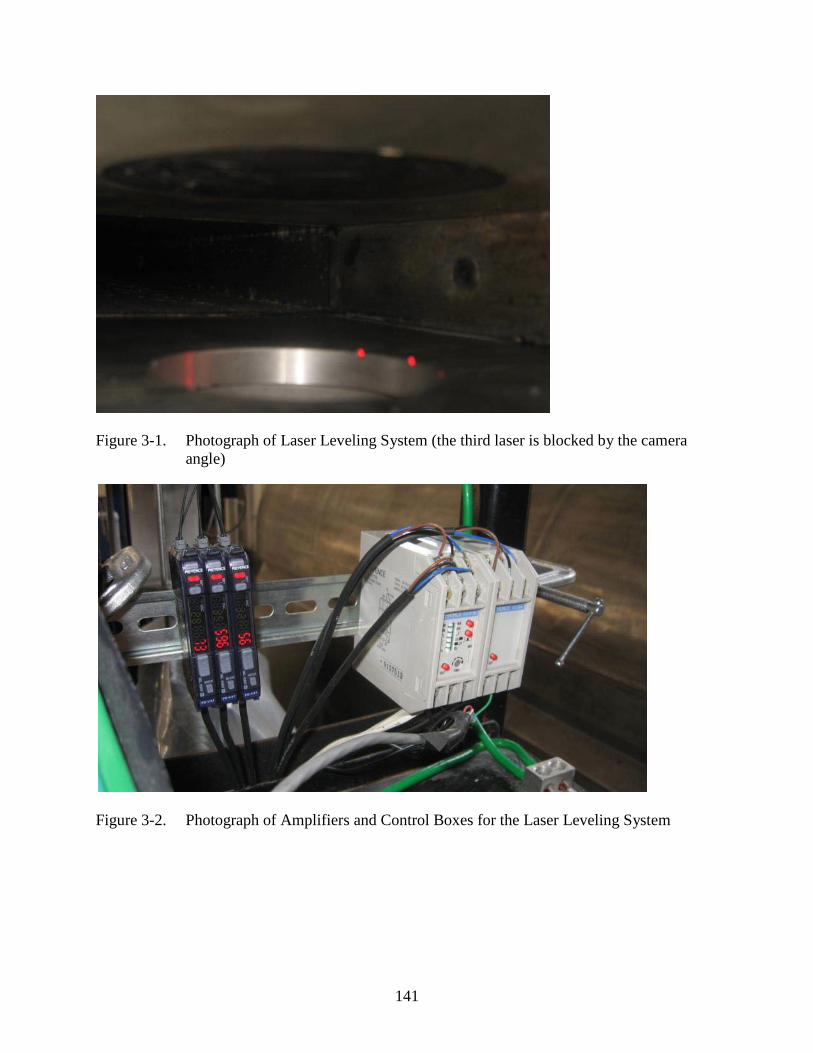
141

Figure 3-1. Photograph of Laser Leveling System (the third laser is blocked by the camera angle)

Figure 3-2. Photograph of Amplifiers and Control Boxes for the Laser Leveling System

142

Figure 3-3. Water Chiller

Figure 3-4. Temperature Drop after Water Chiller Installation

0 20 40 60 80 100 12015

16

17

18

19

20

21

22

23

24

25

Time (Min)

Tem

pera

ture

( o C

)

y(x) = a x + ba = -0.045949b = 24.038R = 0.99509 (lin)

y(x) = a x + ba = -0.05016b = 21.547R = 0.99877 (lin)

143

Figure 3-5. Inner Components of the Shear Stress Sensor

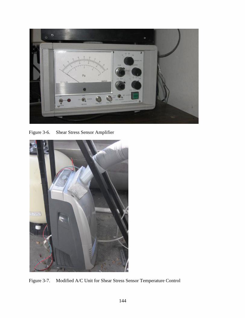
144

Figure 3-6. Shear Stress Sensor Amplifier

Figure 3-7. Modified A/C Unit for Shear Stress Sensor Temperature Control

145

Figure 3-8. Shear Stress Sensor Box with Tube From A/C Unit

Figure 3-9. New Pressure Transducers in SERF

146

Figure 3-10. Trammel’s Original Flow Rate vs. Pump Frequency [Adapted from Trammel, M. A. (2004). “Laboratory apparatus and methodology for evaluating water erosion rates of erodible rock and cohesive sediments.” M.S. thesis, University of Florida, Gainesville, Florida.]

Figure 3-11. New Pump Frequency vs. Velocity Curve

0 10 20 30 40 50 600

1

2

3

4

5

6

7

Pump Frequency (Hz)

Vel

ocity

(m/s

)

y(x) = a xa = 0.10119R = 0.99945 (lin)

147

Figure 3-12. Sand Injector Load Cell Mounts

Figure 3-13. Sand Injector Expansion Joints

148

\

Figure 3-14. Completed Sand Injector

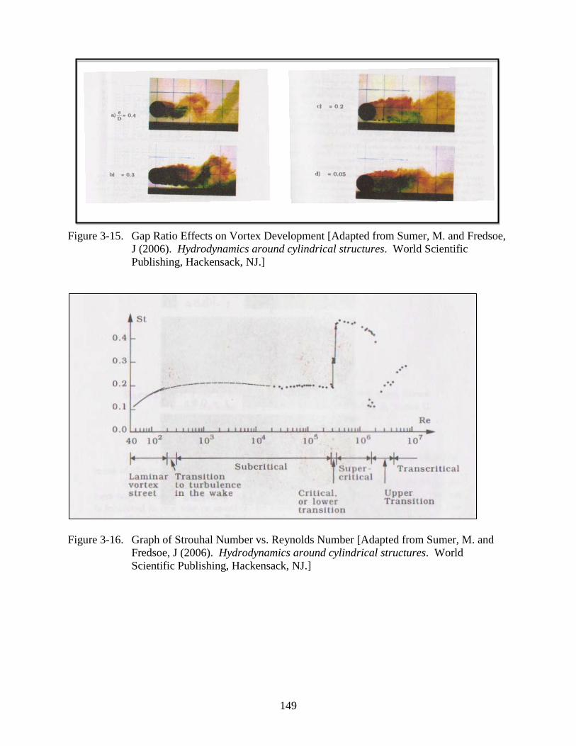
149

Figure 3-15. Gap Ratio Effects on Vortex Development [Adapted from Sumer, M. and Fredsoe, J (2006). Hydrodynamics around cylindrical structures. World Scientific Publishing, Hackensack, NJ.]

Figure 3-16. Graph of Strouhal Number vs. Reynolds Number [Adapted from Sumer, M. and Fredsoe, J (2006). Hydrodynamics around cylindrical structures. World Scientific Publishing, Hackensack, NJ.]

150

Figure 3-17. Vortex Generator installed in SERF (looking into flume)

151

CHAPTER 4 ESTIMATIONS AND MEASUREMENTS OF SHEAR STRESSES ON AN ERODING BED

MATERIAL IN FLUME-STYLE EROSION RATE TESTING DEVICES

4.1 Executive Summary

With the installation of the new shear stress system as described in Chapter 3, a method

was finally available for measuring shear stress directly in a closed rectangular duct and

comparing results with previous methods for estimating shear stresses in a flume. Tests were run

in the SERF for varying bed roughnesses (grain sizes) and at a range of velocities to determine

the accuracy of shear stress estimates using a pressure drop. Tests showed that large particles

can cause higher shear stresses than the returned computed value using a pressure drop. As

particle sizes become smaller, the pressure drop method for estimating shear stress becomes

increasingly more accurate. Relationships were developed for shear stress as a function of

particle size and compared with flat-walled results from the Darcy Weisbach equation and results

obtained using the Colebrook Equation (Moody Diagram) as specified in the EFA. For large

grain sizes, the flat-walled assumption provides poor results. The EFA’s method for estimating

shear stress works better than the flat-wall assumption and the pressure drop if the roughness

height is taken as half the diameter of the eroding particle. When upstream vortices are

artificially induced in the flow field, bed shear stress decreases sharply for a flat bottom, while

shear stress for rough bottoms remains similar to shear stresses under non-vortex conditions.

4.2 Review of Relevant Background

Recall from Chapter 2 that the method for estimating shear stresses in rectangular closed

flumes like the SERF, the EFA, the ASSET, and the SEDFlume relied on estimation techniques.

Shear stress in the ASSSET, the SEDFlume, and the SEAWOLF used the Darcy Weisbach

Equation and a hydraulically smooth assumption to estimate shear stress. In the EFA, friction

152

factor was obtained from a Moody Diagram, the Darcy Weisbach Equation was used, and shear

stress was estimated. Originally in the SERF, a pressure drop was measured and a force balance

was used to solve for shear stress as a function of head differential.

Recall from Chapter 2 that the ASSET, SEDFlume, and SEAWOLF use Equations 4-1, 4-

2, and 4-3 to estimate wall shear stress. These devices make a flat-walled assumption, and

consequently, the friction factor can be solved implicitly.

8.0log0.21−

=

υλ

λUD

(4-1)

wh

hwD+

=2 (4-2)

2

8Uρτλ = (4-3)

In the EFA, Briaud et al. estimate shear stress using Equation 4-3, but their friction factor,

λ, is not solved for using Equation 4-1. Instead, a Moody Diagram is used to estimate this

parameter. The Moody Diagram can be described by the Colebrook Equation:

+−=

λλ Re51.2

7.3/log0.21 De

(4-4)

where e is the roughness height, D is the hydraulic radius of the rectangular duct, and Re is the

Reynolds Number with respect to hydraulic radius. Reynolds Number is given in Equation

4-5while hydraulic diameter is given in Equation 4-6.

whhwD+

=2

(4-5)

νVD

=Re (4-6)

153

where h is the height of the duct, w is the width, and ν is the kinematic viscosity of water.

When examining a cross section of any erosion rate test flume, it becomes clear that the

walls’ roughnesses are not constant. On three sides of the flume, smooth walls are present, but

along the bottom of the flume, a sample with a different roughness is present. Because the

Colebrook Equation and Moody Diagram solve for average friction factor, and these methods

rely on surface roughness, the question becomes which surface height to use when doing these

calculations. Although Briaud does not say what value for ks (or e – these two parameters are

used interchangeably) in his calculations, he implies that this parameter must be a function of

grain size. If one considers how much of a grain will be “exposed” to surface flow when it is

eroding, it makes sense to equate this parameter to precisely one-half of the total average grain

size. Nikraudese verified that this relationship should be correct in rough pipes with a uniform

roughness, but no one has yet to determine if this assumption would be valid for a hydraulic

radius that was mostly smooth with one rough section. Under conditions in flume-style erosion

devices like the SERF, the question became whether or not the Moody Diagram would still be

valid.

Once this question can be answered under steady flow conditions, the next question is how

the presence of vortices affects bed-imposed shear stress (and particle-like erosion since E =

f(τ)). To study the effects of bed shear stress under vortex conditions, the vortex generator was

installed upstream from the shear stress sensor and shear stress measurements were made under

vortex conditions using both the pressure drop and shear stress sensor method.

4.3 Experimental Setup

Appendix B provides in-depth details of how to run a shear stress test in the SERF, but in

brief, the procedure that was used for this study proceeded as follows:

154

1. Experimental discs were prepared for the SERF using the “synthetic” disc preparation method. Crushed limestone was sieved so that particles of 5 diameters – 2.0 mm, 1.0 mm, 0.5 mm, 0.25 mm, and 0.125 mm were isolated from one another. Then, a 50 mm diameter acrylic disc was coated with epoxy and particles from one of the five batches were attached to the front face of the disc. A flat disc was also prepared.

2. An experimental disc was loaded into the shear stress sensor and leveled with the flume bottom.

3. The shear stress sensor was calibrated such that there was a linear relationship between output voltage and shear stress. For example, an output voltage of 10 V indicates a shear stress of 100 Pa; an output voltage of 3 V indicates a shear stress of 30 Pa.

4. Water was run through the SERF to pressurize it, and the pressure transducers were bled to remove any bubbles from their hoses or nozzles. Once the transducers were bled, a 10 second, 1 kHz pressure reading burst was taken at no flow so that a “zero-point” for data analysis could be established.

5. Water was run through the SERF at varying flow rates. Flow rates ranged from 0 m/s to 6 m/s. Data was recorded from the pressure transducers, the shear stress sensor, and the paddlewheel flowmeter at a 1 kHz sampling frequency.

6. Pressure readings were converted to shear stresses using the following relationship:

( )Lwlplw22 +

∆=τ

(4-7)

which is based on a force balance between wall shear stress and an upstream and downstream pressure gradient. Velocity readings were used to compute shear stresses using Equation 4-1 through Equation 4-6.

7. Steps 2 – 6 were repeated for each experimental disc and the flat disc. The result was the development of a relationship between velocity and shear stress for a pressure drop reading, a velocity reading, and a shear stress sensor reading for a given sediment size. Each test was repeated at least four times.

8. A gage pressure transducer was attached to one of the SERF’s pressure ports. Axial stress readings were measured at the specified flow rates.

9. Shear stress tests were repeated with the vortex generator installed. Since the paddlewheel flowmeter was installed upstream from the vortex generator, average velocity readings did not change. Therefore, only the pressure drop and shear stress sensor readings were compared with one another.

155

4.4 Experimental Results and Discussion

4.4.1 Pressure Drop

Tests were first conducted on a flat disc to compare the pressure drop method for

estimating shear stress with actual measurements. The first issue with testing was that

significant noise was present in the pressure transducer signal. While small pressure differential

voltage fluctuations were expected (10-3 V) relatively high pressure differential pressure voltage

fluctuations were observed (10-1 V). Spectral analysis was conducted on the de-meaned signal

from the pressure transducers (Figure 4-1), to determine why these fluctuations were occurring.

There are several noticeable peaks in pressure readings between 5 Hz and 20 Hz. The 65 Hz

spike is electrical noise (120 VAC will produce this) and the 80 Hz and 90 Hz spike were only

present on a few data runs. These are probably due to bubble development at higher flow rates

and effectively can be ignored. The focus then became determining what the 5 Hz – 20 Hz spike

was.

Because shear stress readings were availabe from the sensor, it was possible to find what

the oscillating frequency of the shear stress should have been based on the sensor data by

performing another spectral analysis of shear measurements (Figure 4-2). The shear stress

sensor shows a large spike at approximately 30 Hz. This is most likley the fundamental

vibratory mode of the sensor itself. Recall that the shear stress sensor oscillates back and forth

on its leaf springs. When the sensor is knocked, or water flows over it, it will oscillate at its own

fundamental frequency, and this is probabaly what is causing the 30 Hz spike. If the true

frequency of shear stress readings was at 30 Hz, a similar peak should be seen in Figure 4-1

because frequency should correspond to pressure. Although the correct pressure differential may

not necessarily produce the correct shear stress, one would expect pressure fluctations and shear

stress fluctuations to be similar. This relationship does not exist as demonstrated in these two

156

figures. Therefore, the true data from the shear stress sensor is most likely the block of data seen

in the Figure 4-2 spectograph that lies below 10 Hz. This can be confirmed by isolating the 30

Hz signal using a bandpass filter and plotting a time series of filtered data (Figure 4-3).

The same technique used to isolate the 30 Hz data block from the shear stress sensor was

used to look at the 5 - 20 Hz spike. Specifically, a 5 Hz – 20 Hz 4th order Butterworth bandpass

filter was designed where this data block would be isolated, and another time series was plotted

with transdcuer filtered data (Figure 4-4). The 5 Hz – 20 Hz data block oscillates at

approximately 0 V. This data block then is not the actual signal that needs to be captured.

Rather, it is some vibratory mode that is aliasing the signal. The next thought was that flume

vibration may be causing this fluctuation. Two tests were conducted to rule this out. First, a test

was designed where the pressure transducers were turned on, wired, and hooked up to the SERF.

Then, the control valves from the flume tubing to the transducer were closed so that water could

not cause a pressure differential on the transducer’s membrane. The signal from the pressure

transducers then would be the vibratory mode of the flume (Figure 4-5). As shown, there is no

peak between 5 Hz and 20 Hz. Therefore, the 5 Hz to 20 Hz signal must not be caused by flume

or pump vibrations. The ~45 Hz spike only occurs in one dataset and is not repeated. This could

be due to a number of factors – an air conditioning unit turning on, a fan blowing, someone using

another piece of electrical equipment in the lab, etc. Because it is not repeated and it is not

present under flow conditions, it was ignored. Again, the 65 Hz spike represents electrical noise.

To further confirm that the 5 Hz to 20 Hz vibration must be a “real” signal and not caused

by pump or vibrational noise, the pressure transducer was removed from the SERF frame and

attached to the external frame that holds the sample into place. Doing this eliminated most

vibrations from the transducer. Data was taken at three flow rates because this data was taken

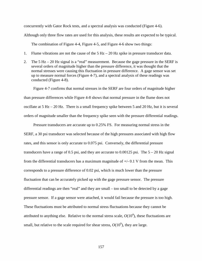
157

concurrently with Gator Rock tests, and a spectral analysis was conducted (Figure 4-6).

Although only three flow rates are used for this analysis, these results are expected to be typical.

The combination of Figure 4-4, Figure 4-5, and Figure 4-6 show two things:

1. Flume vibrations are not the cause of the 5 Hz – 20 Hz spike in pressure transducer data.

2. The 5 Hz – 20 Hz signal is a “real” measurement. Because the gage pressure in the SERF is several orders of magnitude higher than the pressure difference, it was thought that the normal stresses were causing this fluctuation in pressure difference. A gage sensor was set up to measure normal forces (Figure 4-7), and a spectral analysis of these readings was conducted (Figure 4-8).

Figure 4-7 confirms that normal stresses in the SERF are four orders of magnitude higher

than pressure differences while Figure 4-8 shows that normal pressure in the flume does not

oscillate at 5 Hz – 20 Hz. There is a small frequency spike between 5 and 20 Hz, but it is several

orders of magnitude smaller than the frequency spike seen with the pressure differential readings.

Pressure transducers are accurate up to 0.25% FS. For measuring normal stress in the

SERF, a 30 psi transducer was selected because of the high pressures associated with high flow

rates, and this sensor is only accurate to 0.075 psi. Conversely, the differential pressure

transducers have a range of 0.5 psi, and they are accurate to 0.00125 psi. The 5 – 20 Hz signal

from the differential transducers has a maximum magnitude of +/- 0.1 V from the mean. This

corresponds to a pressure difference of 0.02 psi, which is much lower than the pressure

fluctuation that can be accurately picked up with the gage pressure sensor. The pressure

differential readings are then “real” and they are small – too small to be detected by a gage

pressure sensor. If a gage sensor were attached, it would fail because the pressure is too high.

These fluctuations must be attributed to normal stress fluctuations because they cannot be

attributed to anything else. Relative to the normal stress scale, O(104), these fluctuations are

small, but relative to the scale required for shear stress, O(100), they are large.

158

Data was collected over a 10 s time interval at a frequency of 1 kHz, and then averaged

over the time domain. Because the 5 Hz – 20 Hz frequency band averages to zero, for the

purposes of averaging, it could be ignored. If one wanted to eliminate this noise band, it would

be possible using a longer flume length, but modifications would be required. Pressure could be

measured higher upstream and further downstream than it currently is measured. Currently the

pressure difference is only measured +/-2 inches from the sample because the goal is to isolate

the sample’s effect on pressure difference. With the flume’s present setup, if the pressure ports

were spaced further apart, a larger portion of the pressure difference would be caused by the

flume walls, while a smaller relative portion of the pressure differential would be caused by the

eroding sample roughness. On average then, a higher portion of the overall average shear stress

would be computed from walls – thereby theoretically throwing the calculation for shear stress

across the face of the sample off even further.

The word “theoretically” is used in the preceding paragraph because the rationale behind

the original spacing of the SERF pressure ports was to space them close to the sample so that the

sample’s effects on pressure differential would be maximized. In other words, pressure ports

were spaced just upstream and just downstream from the sample because the sample is rougher

than the flume walls. The rougher sample should produce an overall higher pressure differential

effect on its respective flume portion. As pressure ports are spaced further from the sample

locus, there will be more flat flume area relative to the amount of rough sample area (which must

remain constant). This increase in relative smooth area should cause the pressure differential to

behave more like a “smooth” pressure differential and less like a “rough” pressure differential.

Unfortunately, even with close pressure port spacing, the sample’s effect on pressure

differential (and subsequently shear stress) was minimal. To illustrate this, a series of discs with

159

different uniform grain sizes – 2 mm, 1 mm, 0.5 mm, 0.25 mm, and 0.125 mm – were prepared

by sieving crushed limestone through several ASTM standard sieves and gluing these particles to

50 mm shear stress sensor discs. Prefabricated 50 mm discs acrylic discs with a predrilled hole

through the center were purchased, attached to the shear stress sensor and the SERF run at

varying flow rates. Spectral analyses for these rough discs were similar to spectral analyses

presented for flat discs and will not be repeated. Namely, there are zero-mean pressure

fluctuations in the device that are probably caused by a small-scale axial stress fluctuation.

Comprehensive results of different diameter tests will be presented in Section 4.4.2 so that they

can be compared with analytical methods for estimating shear stress, but with respect to

estimating shear stress via the pressure transducer, Figure 4-9 is an illustration of what is

happening in the SERF.

As roughness of the shear stress sensor’s disc changed from smooth under flat conditions

to rough under large sediment conditions, the shear stress estimate from the pressure transducers

did not change. It appears as though the sample area relative to the flat flume wall area is too

small to see a noticable effect on average pressure difference in the flume. Figure 4-9 can be

constrasted with Figure 4-10 to show the actual shear stress measurements across the face of the

sample from the shear stress sensor. Figure 4-10 shows that as roughness (sediment size)

increases, shear stress increases signficinatly. Therefore, using a pressure drop to estimate shear

stress for a rough sample would underestimate the actual shear stress conditions because on

average, the pressure drop is influenced more by the contributing area of the flat wall cross

sectional area than it is by the rough sediment disc cross sectional area.

If one wanted to use a pressure differential to estimate shear stress, it would be possible if

conditions in the SERF were different. The Moody diagram was developed by measuring

160

pressure differences in uniformly rough pipes. A similar technique could be used to predict

shear stresses in a flume like the SERF – wall inserts would need to be constructed where

different size diameter sediments were used. This would provide accurate pressure drop

readings. However, in its present setup, because the SERF has flat walls and because the area of

the test section (and shear sensor) is so small relative to the area of the flat walls, estimating

shear stress from a pressure drop will not produce accurate results.

The implications of this for previous SERF tests are interesting. Several erosion rate-shear

stress curves have already been developed for materials that should not be considered flat (Gator

Rock in particular). Because of this, the shear stresses used in development of these curves must

be too small, and should be modified.

4.4.2 Analytical Methods

Once the question of shear stress estimation using a pressure drop had been assessed, the

other methods for estimating shear stress were investigated (Figure 4-11 through Figure 4-17).

Figure 4-18 is a nondimensionalized summary of data, and probably provides the most concise

method for analyzing results. Even though the Moody Diagram in the closest alternative

technique for estimating shear stress, it is still produces some error. Figure 4-18 is a diagram

that shows % Error vs. Reynolds Number. Results show three things:

1. Estimating shear stress from a pressure drop will over predict shear stress under flat conditions.

2. Estimating shear stress from a flat-walled approach will underestimate shear stress as grain size increases.

3. Estimating shear stress with the Colebrook Equation is the most accurate alternative technique if effective roughness is assumed to be one-half the sediment diameter.

At low Reynolds Numbers, the percent error is high, but the shear stress magnitude is low.

Therefore, this should not be a major concern. The largest errors occur for the smoothest test

161

discs. The 1.37x10-8 value for ks for a smooth disc was obtained from the literature, so it is not

reflective of the experimental technique. The next largest source of error was for the 0.125 mm

grain size. Since errors approach zero for this test disc as Reynolds Number increases (and shear

stress magnitude increases), the high overestimation of friction factor should not be a huge

concern either. For larger diameter grain sizes, error is low; as Reynolds Number becomes

greater than 1x105, error is less than 20% when grain size is 0.25 mm or greater. Because the

larger diameter specimens show the highest shear stress magnitudes, presumably these

estimations are the most important.

4.4.3 Vortex Conditions

Another goal of this study was to determine how the introduction of vortices influences

erosion rate-shear stress curves. As discussed in the literature review, for particle-like erosion

there is both a theoretical basis for quantifying erosion rate as a function of shear stress and a

history of empirical relationships between these two parameters. When investigating the effects

of vortices, preliminarily, it appears as though the vortex itself should not be studied, especially

since at present a velocity profile cannot be measured in the SERF. Rather, the effect of the

vortex on average shear stress should be studied, and because erosion rate is a function of shear

stress, erosion rate effects of vortices would follow. Preceding tests on uniform diameter

experimental discs were repeated with the SERF’s vortex generator installed. Results are

presented from Figure 4-19 through Figure 4-26. In general, the induction of upstream vortices

in the SERF appears to produce on average lower shear stresses for a given velocity. These

effects appear to become magnified as particle size decreases. For larger particles (1 mm and 2

mm), the effects of vortices are nearly negligible.

Qualitatively, this particle-dependency on vortex effects makes sense. Large particles are

going to produce their own vortices, and introducing a large upstream vortex (wake region)

162

should have a minimal effect when compared with the effects of the vortices caused by the

roughness of the sample. Conversely, small particles will not produce large vortices on their

own. Therefore, they are more affected by the shearing action of water against their surface and

less affected by vortex-particle interaction. As such, when a large upstream vortex is induced in

the SERF, its net effect from the perspective of a small particle is simply to retard the flow in the

direct vicinity of a small particle, thereby decreasing the net overall shearing action against it.

Large particles on the other hand are more affected by local vortex affects, and a small net-

retardation of the flow will produce little shear stress effect.

Because in general vortex induction lowers shear stress, and because particle-like erosion

rate is intrinsically tied to shear stress, under vortex conditions, particle-like erosion rate should

decrease proportionally with shear stress. This could be useful under field conditions where a

large obstruction is directly upstream from a bridge pier (a large pipe for example). The design

shear stress may be able to be reduced by a factor proportional to particle size. To be

conservative however, even under vortex conditions, non-vortex shear stress (and erosion rates)

should be used until field verification of this can be made.

4.5 Recommendations and Conclusions

In summary, from this it appears as though the shear stress question in the SERF has been

solved. The following are recommendations and conclusions from this study:

1. For a rough sample, a pressure drop may not be used to estimate shear stress because it will under predict actual shear stress conditions

2. For a flat sample, the method used in the ASSET, SEDFlume, and SEAWOLF may be used to predict shear stress. The EFA method may also be used with a small roughness height.

3. For a rough sample, the ASSET/SEDFlume/SEAWOLF method should not be used because it will under predict shear stress.

163

4. For a rough sample, the EFA method may be used, but the roughness height should be one-half the particle diameter.

5. If the correct roughness is not known (for example with a rock or non-uniform sediment), an estimation based on largest particle diameter should be used.

6. Vortices appear to have a small overall effect on average shear stress development.

7. For large particles, upstream vortices have a minimal effect.

8. For small particles, upstream vortices have a larger effect, and they generally reduce net overall average shear stress.

4.6 Future Work

The equivalent roughness concept may help future flume-style shear stress testing. This

can be viewed similarly to equivalent diameters for bridge piers as presented in the FDOT bridge

scour manual. In other words, even though a rock core or sand-clay mixture may not have a

specific grain size associated with it from a bulk sense (as would be common with natural

samples), it may be possible to measure its surface roughness and assign an equivalent grain size

that can be used to predict the shear stress from a Moody Diagram.

Although not in the scope of this project, there is a device at UF called AIMS that can

measure the roughness of a series of concrete cores using high resolution cameras. The AIMS

can be modified so that it can measure the roughness of rock cores or sand-clay samples. As

demonstrated in this chapter, roughness should be equivalent to one-half the grain size, and in

the case of rock and non-uniform mixtures, it appears as though this relationship should hold true

as well.

This chapter has shown that producing the correct shear stress in a flume-style erosion rate

testing device is critical in measuring the correct erosion rate for an erosion rate-shear stress

curve. Shear stress is inherently tied to grain size, or roughness, and without proper stress-

estimation in the SERF, improper erosion rates will be computed. When dealing with an intact

164

rock core or natural sand-clay sample, it is essential to “know” what shear stress is actually being

applied to it so that the correct erosion rate relationship can be developed. Future AIMS testing

appears to be a possible solution as a link between intact rock core roughness and future SERF

testing.

165

Figure 4-1. Spectral analysis of de-meaned pressure transducer voltages

Figure 4-2. Spectral analysis of de-meaned shears stress sensor measurements.

0 10 20 30 40 50 60 70 80 90 1000

0.05

0.1

0.15

0.2

0.25

0.3

0.35

0.4

Frequency (Hz)

Spe

ctra

l Den

sity

Spectral Analysis of Pressure Transducer Signals

0 10 20 30 40 50 60 70 80 90 1000

10

20

30

40

50

60

70

80

90

100

Frequency (Hz)

Spe

ctra

l Den

sity

Spectral Analysis of Shear Sensor Signals

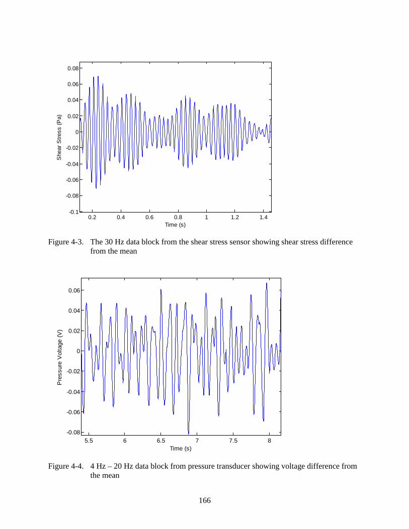
166

Figure 4-3. The 30 Hz data block from the shear stress sensor showing shear stress difference

from the mean

Figure 4-4. 4 Hz – 20 Hz data block from pressure transducer showing voltage difference from

the mean

0.2 0.4 0.6 0.8 1 1.2 1.4-0.1

-0.08

-0.06

-0.04

-0.02

0

0.02

0.04

0.06

0.08

Time (s)

She

ar S

tress

(Pa)

5.5 6 6.5 7 7.5 8-0.08

-0.06

-0.04

-0.02

0

0.02

0.04

0.06

Time (s)

Pre

ssur

e V

olta

ge (V

)

167

Figure 4-5. Spectral analysis of free-vibratory flume test voltage measurements

Figure 4-6. Spectral analysis of free-vibratory flume test with sensor on new frame

0 10 20 30 40 50 60 70 80 90 1000

0.005

0.01

0.015

0.02

0.025

Frequency (Hz)

Spe

ctra

l Den

sity


0 5 10 15 20 25 30 35 40 45 500

0.005

0.01

0.015

0.02

0.025

0.03

Frequency (Hz)

Spe

ctra

l Den

sity


168

Figure 4-7. Average normal stresses in the SERF

Figure 4-8. Spectral analysis of normal stresses

1 2 3 4 5 60

0.5

1

1.5

2

2.5

3

3.5

4

x 104

Nor

mal

Stre

ss (P

a)

V (m/sec)

10 20 30 40 50 60 70 80

0.5

1

1.5

2

2.5

3

3.5

4

4.5x 10

-3

Frequency (Hz)

Spe

ctra

l Den

sity


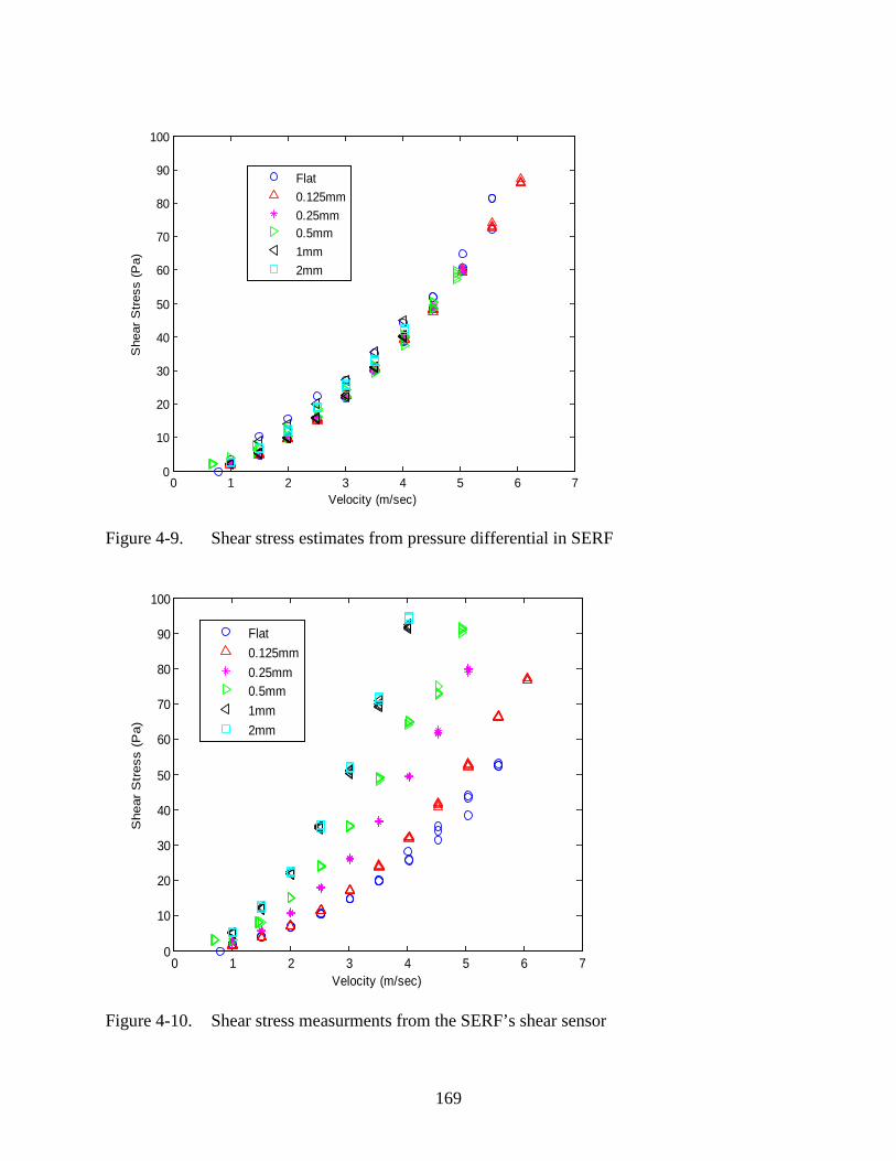
169

Figure 4-9. Shear stress estimates from pressure differential in SERF

Figure 4-10. Shear stress measurments from the SERF’s shear sensor

0 1 2 3 4 5 6 70

10

20

30

40

50

60

70

80

90

100

Velocity (m/sec)

She

ar S

tress

(Pa)

Flat0.125mm0.25mm0.5mm1mm2mm

0 1 2 3 4 5 6 70

10

20

30

40

50

60

70

80

90

100

Velocity (m/sec)

She

ar S

tres

s (P

a)


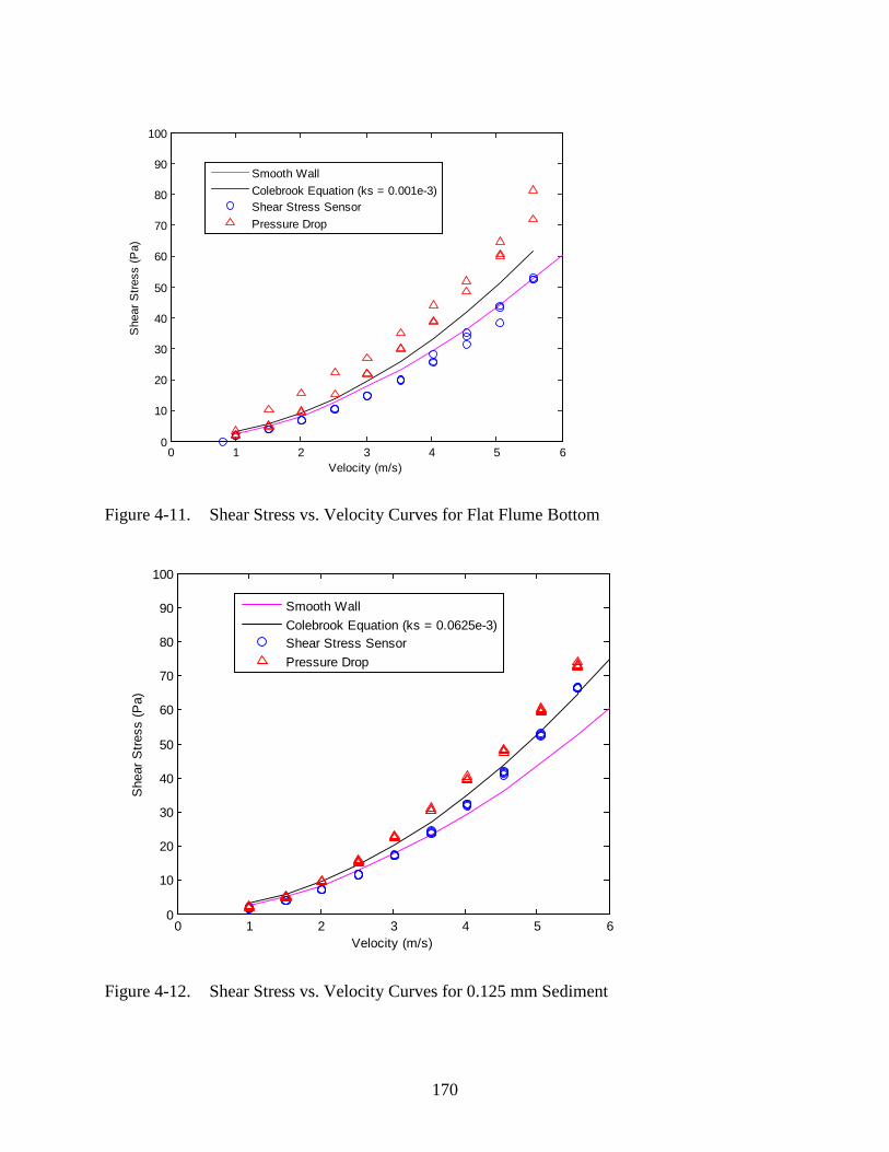
170

Figure 4-11. Shear Stress vs. Velocity Curves for Flat Flume Bottom

Figure 4-12. Shear Stress vs. Velocity Curves for 0.125 mm Sediment

0 1 2 3 4 5 60

10

20

30

40

50

60

70

80

90

100

Velocity (m/s)

She

ar S

tress

(Pa)

Smooth WallColebrook Equation (ks = 0.001e-3)Shear Stress SensorPressure Drop

0 1 2 3 4 5 60

10

20

30

40

50

60

70

80

90

100

Velocity (m/s)

She

ar S

tress

(Pa)


171



0 1 2 3 4 5 60

10

20

30

40

50

60

70

80

90

100

Velocity (m/s)

She

ar S

tress

(Pa)


0 1 2 3 4 5 60

10

20

30

40

50

60

70

80

90

100

Velocity (m/s)

She

ar S

tress

(Pa)


172



0 1 2 3 4 5 60

10

20

30

40

50

60

70

80

90

100

Velocity (m/s)

She

ar S

tress

(Pa)


0 1 2 3 4 5 60

10

20

30

40

50

60

70

80

90

100

Velocity (m/s)

She

ar S

tress

(Pa)

Smooth WallColebrook Equation (ks = 1e-3)Shear Stress SensorPressure Drop

173

Figure 4-17. Combined Non-Dimensionalized Results From Colebrook Equation, Shear Readings, and Smooth-Wall Assumption (dashed line is smooth wall).

Figure 4-18. Percent error vs. Reynolds Number between Colebrook Equaiton using a Uniform

Roughness and Actual Shear Stress Measurments

0 0.5 1 1.5 2 2.5 3 3.5 4 4.5

x 105

0

0.01

0.02

0.03

0.04

0.05

0.06

0.07

Re

f

e/D=6.85e-9e/D=8.55e-4e/D=1.72e-4e/D=1.92e-3e/D=6.85e-3e/D=1.37e-2Smooth Bottom

0.5 1 1.5 2 2.5 3 3.5 4 4.5

x 105

0

20

40

60

80

100

120

Re

Per

cent

Diff

eren

ce

e/D=1.37e-8e/D=1.71e-3e/D=3.43e-3e/D=6.85e-3e/D=1.37e-2e/D=2.74e-2

174

Figure 4-19. Combined Shear Stress Sensor Data Under Vortex Conditions

Figure 4-20. Comparison of Pressure Readings for Vortex and Non-Vortex Conditions for all Sediment Diameters

0 1 2 3 4 5 6 70

10

20

30

40

50

60

70

80

90

100

Velocity (m/sec)

She

ar S

tress

(Pa)


0 1 2 3 4 5 6 70

10

20

30

40

50

60

70

80

90

100

Velocity (m/s)

She

ar S

tress

(Pa)

With VorticesWithout Vortices

y(x) = a x n̂a = 1.0005n = 2.3806R = 0.92757 (lin)

y(x) = a x n̂a = 2.9275n = 1.8773R = 0.99666 (lin)

175

Figure 4-21. Comparison between Shear Stress Readings for Flat Bottom under Vortex and Non-Vortex Conditions

Figure 4-22. Comparison between Shear Stress Readings for 0.125 mm Sediment under Vortex and Non-Vortex Conditions

0 1 2 3 4 5 6 70

10

20

30

40

50

60

70

80

90

100

Velocity (m/s)

She

ar S

tress

(Pa)


0 1 2 3 4 5 6 70

10

20

30

40

50

60

70

80

90

100

Velocity (m/s)

She

ar S

tress

(Pa)


176



0 1 2 3 4 5 6 70

10

20

30

40

50

60

70

80

90

100

Velocity (m/s)

She

ar S

tress

(Pa)


0 1 2 3 4 5 6 70

10

20

30

40

50

60

70

80

90

100

Velocity (m/s)

She

ar S

tress

(Pa)


177



0 1 2 3 4 5 6 70

10

20

30

40

50

60

70

80

90

100

Velocity (m/s)

She

ar S

tress

(Pa)


0 1 2 3 4 5 6 70

10

20

30

40

50

60

70

80

90

100

Velocity (m/s)

She

ar S

tress

(Pa)


178

CHAPTER 5 DEVELOPMENT AND TESTING WITH A NEARLY UNIFORM, HIGHLY ERODIBLE, SYNTHETIC ROCK-LIKE MATERIAL TO BE USED FOR CALIBRATING EROSION-

RATE TESTING DEVICES


Because of questions in comparing Rotating Erosion Test Apparatus (RETA) results with

more traditional flume-style erosion rate test devices results, attempts were made to develop a

nearly uniform material to serve as a direct comparison medium between these different

instruments. A new material, Bull Gator Rock, was developed using similar principles to older

Gator Rock designs. While older versions of Gator Rock were mixed with water, Bull Gator

Rock was mixed dry and water was added to the mix later through capillary action. Two

different rounds of Bull Gator Rock mix were developed. The first round showed excellent

compressive and tensile strength test results. Erosion results in the RETA and the Sedimentary

Erosion Rate Flume (SERF) were mixed. Cement content and water content were increased, and

a second round of Bull Gator Rock was produced. Because of aggregate variability, strength

tests were not repeatable. Erosion tests showed the presence of rock-like erosion, although a

promising result from one round of testing showed the potential for a particle-dominated erosion

scenario. Eventually, researchers realized that for a direct RETA-to-flume style device

comparison, an extensive dataset was required.


Because the RETA measures erosion on a rock core or Shelby tube’s sides instead of on its

top surface, people have questioned whether or not results from these erosion tests were the same

as they would have been had a more traditional flume-style device been used instead. When this

project began, the first thought was that the most effective way to verify that the RETA was to

directly compare RETA results to results from a flume-style device. The Sediment Erosion Rate

179

Flume (SERF) was used as the flume-style device in this study. To perform this comparison, a

suitable material was needed for testing in both instruments.

Finding a naturally occurring material that is erodible in both the SERF and the RETA is

not as easy as it sounds. Any material to be tested in both devices needs to have enough internal

strength to withstand moment forces associated with the RETA. Materials like soft clay and

compacted sands will often crumble during RETA testing, and these results are useless when

trying to compare the two devices. Despite this internal strength criterion, the material to be

tested in both devices also needs to be highly erodible. Any material to be tested in both devices

must be nearly uniform. A non-uniform sample will become obvious during a RETA test, as one

localized section of the sample will erode faster than another section. The material tested in both

devices must also be uniform from another standpoint – from sample to sample. Repeatability of

erosion and strength test data is important because if one can differentiate one sample from

another, any results coming from a comparison will be meaningless.

Because of these stringent criteria for testing a material in the RETA and the SERF, work

to compare results from the two devices in the past has focused on the use of synthetic materials.

Niraula’s (2004) Gator Rock was used as a starting point because previous researchers,

particularly Slagle (2006) indicated that he believed Gator Rock could serve as a proper material

for testing in both instruments. Although the original version of Gator Rock was too strong,

Slagle believed that by raising the water content, he could create a nearly uniform material that

was strong enough to withstand RETA testing while still eroding.

As discussed in Chapter 2, Slagle’s original attempt to create Gator Rock was problematic.

He mixed water, crushed limestone, and cement in the appropriate proportions, and allowed the

samples to cure for 28 days. Then, the samples were subjected to RETA testing.

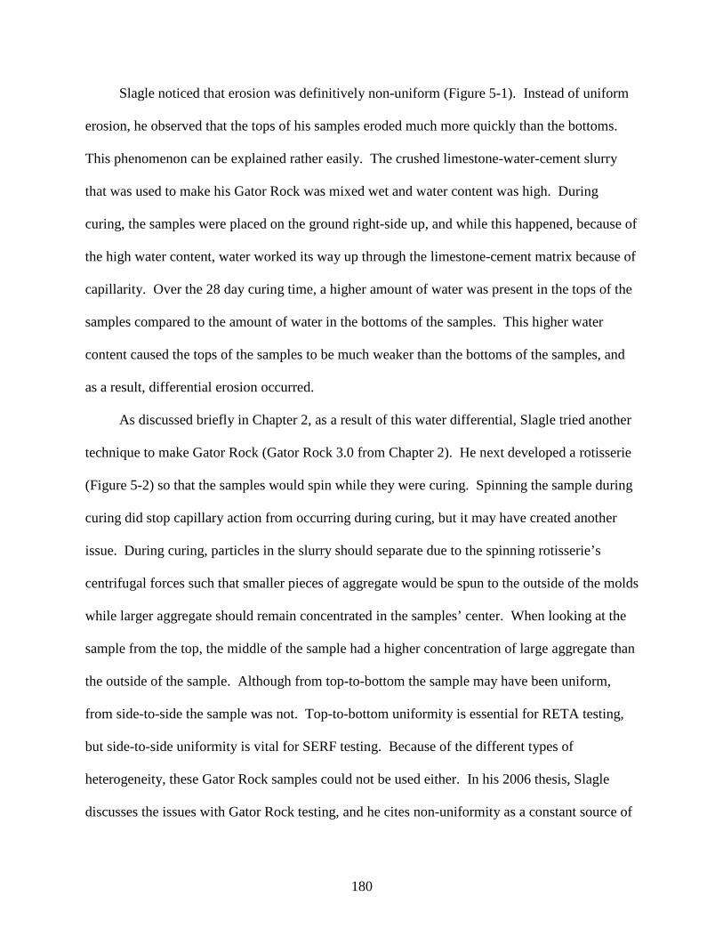
180

Slagle noticed that erosion was definitively non-uniform (Figure 5-1). Instead of uniform

erosion, he observed that the tops of his samples eroded much more quickly than the bottoms.

This phenomenon can be explained rather easily. The crushed limestone-water-cement slurry

that was used to make his Gator Rock was mixed wet and water content was high. During

curing, the samples were placed on the ground right-side up, and while this happened, because of

the high water content, water worked its way up through the limestone-cement matrix because of

capillarity. Over the 28 day curing time, a higher amount of water was present in the tops of the

samples compared to the amount of water in the bottoms of the samples. This higher water

content caused the tops of the samples to be much weaker than the bottoms of the samples, and

as a result, differential erosion occurred.

As discussed briefly in Chapter 2, as a result of this water differential, Slagle tried another

technique to make Gator Rock (Gator Rock 3.0 from Chapter 2). He next developed a rotisserie

(Figure 5-2) so that the samples would spin while they were curing. Spinning the sample during

curing did stop capillary action from occurring during curing, but it may have created another

issue. During curing, particles in the slurry should separate due to the spinning rotisserie’s

centrifugal forces such that smaller pieces of aggregate would be spun to the outside of the molds

while larger aggregate should remain concentrated in the samples’ center. When looking at the

sample from the top, the middle of the sample had a higher concentration of large aggregate than

the outside of the sample. Although from top-to-bottom the sample may have been uniform,

from side-to-side the sample was not. Top-to-bottom uniformity is essential for RETA testing,

but side-to-side uniformity is vital for SERF testing. Because of the different types of

heterogeneity, these Gator Rock samples could not be used either. In his 2006 thesis, Slagle

discusses the issues with Gator Rock testing, and he cites non-uniformity as a constant source of

181

concern. He does not specifically say how his samples were heterogeneous, but from the

mechanisms just described, one can infer how it must have happened.

As of 2006, no known material had been developed that was appropriate for a SERF-vs.-

RETA comparison. In this study, another attempt was made to create a new version of Gator

Rock that would meet the stringent material criteria for SERF-RETA tests and that could be

easily and inexpensively mass-produced.

5.3 Theory Behind Bull Gator Rock

In this study, a new tactic was used to construct Gator Rock. The rotisserie idea was

abandoned, and instead, researchers looked to take advantage of the water’s capillarity. Because

capillary action occurs slowly, researchers hypothesized that cement and crushed limestone

could be mixed dry, the dry mix could be placed in a specific amount of water, and over time, the

water would work its way up through the sample much like it did during the first attempt to make

Gator Rock. As the water worked its way through the sample slowly, a new, nearly uniform

Gator Rock specimen should be created.

In principle this mixing technique had the potential to have the opposite effect as the

original Gator Rock recipe. Because the Gator Rock sample was mixed dry, and water was

added to it from the bottom, one could argue that the bottom of the sample would entrain more

water than the top of the sample. If capillary forcing of the water was not higher than the force

of gravity, indeed, this argument would make sense. A smaller quantity of water could be

transferred to the top of the sample while a larger quantity of water would remain at the sample’s

bottom. However, during the original attempt to make Gator Rock, the opposite was seen. The

tops of the samples, not the bottoms were locally the weakest. Therefore, it was known that

capillary forces in the crushed limestone-cement matrix were relatively high, and researchers

thought that this dry-mix technique would produce a nearly uniform sample.

182

5.4 Procedure for Construction of “Bull Gator Rock”

The following procedure for development of Bull Gator Rock was developed by Crowley,

Bloomquist, and Shah; it was originally presented in Shah’s Honor’s Thesis in 2009, but since

then, some modifications have been made to the process. The finalized process in presented

below:

1. Crushed limestone was obtained from the Whitehurst Company’s mine in Newberry, FL (FDOT Reference No. 34-104), and oven dried for 72 hours.

2. Dried material was sieved through a standard ASTM No. 10 sieve to eliminate cobbles and larger pieces of aggregate.

3. 4 inch molds were cut from standard PVC pipe. For RETA testing, completed Gator Rock samples must have a final diameter of 2.40 inches while for SERF tests, samples must have a final diameter of 2.30 inches. Therefore, when samples were prepared for use in the RETA, standard 2.5 inches SCH 40 pipe was used; when samples were prepared for use in the SERF, standard 2.5 inches SCH 80 PVC pipe was used.

4. Micro filter paper was glued to the molds’ bottoms and the molds’ sides were coated with prestress mold release to prevent the samples from sticking to the molds’ sides.

5. Water-cement ratios were chosen for the Bull Gator Rock batches. Then the appropriate amounts of water, cement, and water were determined using the following formulas:

TotalLimestone M

CLSLSM

+=

%%% (5-1)

TotalCement M

CLSCM

+=

%%%

(5-2)

( )CementLimestoneWater MM

WWM +

−=

%1%

/ (5-3)

In these equations, %LS is the percentage limestone per batch, %C is the percentage cement per batch, and %W is the percentage water per batch. To estimate MTotal or the total mass of the entire Gator Rock batch, a mold was filled with crushed limestone, rodded, and weighed to determine the approximate total mass of substance that could be fit into a mold. Then, this weight was multiplied by the number of samples to be made. For example, if 40 samples were to be made, and the mass of crushed limestone that would fit inside of a mold was approximately 475 g (which was typical for a SCH 40 mold), then MTotal = (40*475 g) = 19 kg.

183

6. A cement mixer was cleaned and dried. Limestone and cement were added to the mixer in the appropriate quantities. To prevent fines from escaping during mixing, a plastic bag was used to seal the cement mixer. The cement mixer was turned on, and mixing lasted for 10 minutes.

7. Molds were prepared.

8. First, an empty mold was weighed.

9. A collar was secured over the mold, and the dry mix was poured into the mold.

10. When the cement-limestone mix was approximately 2.5 inches from the top of the collar, pouring ceased, and the sample was gently leveled.

11. A plastic disc was placed in the 2.5 inches void to seal the contents of the mold. The disc was included so that during vibrating, the fines would not escape.

12. Samples were placed on a shake table with a 3.6 kg mass resting over each sample’s plastic disc. The shake table was set to a speed of 2 and allowed to run for 8 minutes. This insured a densely packed dry mix.

13. The collar was removed, and pressure was applied to the plastic disc. Excess material was scraped from the top of the mold using a screed. The sample (with the mold) was weighed.

14. During SERF tests, it is useful to have an anchor to hold the sample to the piston. During high flow rates in the flume, the pressure differential caused by high velocities in the flume causes the sample to be “sucked” to the flume’s top. For samples to be used in the SERF then, a 2.5 inch x 0.25 inch diameter bolt was inserted into the dry-mix. A 1.0 inch pilot hole was first manually drilled, the bolt was inserted, and the void was back-filled and tampered by hand.

15. Because RETA testing requires the presence of a 0.25 inch hole through the sample, for samples that were to be used for RETA testing, a 0.25 inch aluminum bar was coated with Prestress Release and driven through the samples. This step was added because drilling through a Gator Rock specimen with a drill press may cause the sample to crack. A similar technique to the technique used in (10) was used to insert these rods into the samples.

16. Samples were placed in buckets to allow for curing. The appropriate amount of distilled water was weighed and placed into each curing container. Each bucket was sealed to prevent evaporation during curing. Originally, plastic wrap and Duct Tape were used to seal the buckets, but later, buckets were replaced with Ziploc containers with air-tight lids.

17. Samples were allowed to cure for 28 days.

184

5.5 First Gator Rock Mix

5.5.1 Mix Compositions

During this project, two different versions of Gator Rock were created. The first version of

Gator Rock was based on Niraula’s 2002 original mixing procedure. According to Niraula,

when he changed water-cement ratios, he fixed his water content at 20%, and he varied the

cement content (Table 5-1). Slagle did not indicate which water-cement ratios he used during his

tests. Because Niraula was the only other available reference for Gator Rock, the same thing was

done, and water content was fixed at 20%. To make samples weaker than Niraula’s, cement

content was reduced while Limestone content was increased (Table 5-2).

Before mixing, four random limestone aggregate samples were taken and sieved so that a

grain size distribution could be produced. If random samples showed repeatability and regular

uniformity, it was thought that there would be a better chance to insure that results from one

sample could be compared with results from another sample. As shown (Figure 5-3) the four

random grain size distributions were close to one another.

5.5.2 Strength Tests

After curing had been completed, a random set of Bull Gator Rock samples were selected

for tensile and compressive strength testing. Two samples from each batch were used in each

test. Results from tensile and compressive strength tests were used to compute cohesion for each

batch of Gator Rock according to the formula derived in Chapter 2 (Figure 5-4):

tuqqC21

= (5-4)

where qu is the material’s compressive strength and qt is the material’s tensile strength.

As shown in Figure 5-3, repeatability from sample to sample of the same batch was

excellent. Average percent difference between one sample and another of the same batch during

185

tensile strength testing was 5.86%. Maximum difference from one sample to another during

tensile strength testing was 12.86% (Batch 2); the minimum difference was 2.00% (Batch 1).

The standard deviation of percentage difference between samples of the same batch was 4.37%.

During compressive strength, the average percent difference between samples of the same

batch was 5.25%. The maximum difference from one sample to another of the same batch

during compressive testing was 9.09% (Batch 2); the minimum difference was 0.22% (Batch 4).

The standard deviation of percent difference between samples of the same batch was 3.95%.

5.5.3 RETA Tests

RETA tests were conducted at the FDOT State Materials Office (SMO). Testing followed

the standard RETA testing procedure. The only difference between RETA tests conducted

during this study and typical RETA tests was that because the Gator Rock samples were

artificially created and allowed to cure in molds, their side-walls were abnormally smooth.

Therefore, before each test, the Gator Rock samples were slightly machined so that

approximately 0.1 inches of material was removed from their smooth surface. This artificial

procedure roughened the surfaces slightly. Overall, RETA tests produced mixed results.

5.5.3.1 First round of tests on first batch of Gator Rock in RETA

The first round of samples that were tested produced encouraging results. Dan Pitocchi

(2010), the SMO’s lab technician who oversees FDOT RETA tests, indicated that these Bull

Gator Rock samples were the best Gator Rock samples that he had ever worked with because

from top to bottom, they appeared to erode uniformly. Unlike Slagle’s samples (Figure 5-3)

there were not obvious weaker sections on either the tops or the bottoms of the samples (Figure

5-5, Figure 5-6, and Figure 5-7).

During the first round of testing, quantitative results showed what was expected in terms of

an erosion rate-shear stress relationship. Generally, as shear stress increased, erosion rate

186

increased (Figure 5-8, Figure 5-9, and Figure 5-10). A best-fit line was fit to each dataset using

linear regression. As shown in Figure 5-8, the 10 Pa data point is higher than most other data

points. Often, when a RETA test begins, RETA operators run the lowest shear stress first and

increase the stress every specified time period (24-hours for these tests). Recall that as part of

preconditioning, these samples were slightly machined. The standard RETA testing procedure

calls for a quick wash of the material before data is taken. During the wash a high shear stress is

used to remove any loose particle or debris from the sample. Then, RETA’s annulus is emptied,

cleaned, and the data run begins.

This washing technique does remove some loose particles from the sample. However, if

erosion is rock-like, which for Gator Rock it may be, then this washing technique also serves to

loosen or weaken some grains within the sample matrix. During the sample’s first prolonged

exposure to stresses – normal or shear – these loosened pieces of material will also break off

over time. Therefore, during a 24-hour test, one should expect that some of the looser, exterior

particles that comprise the sample will fall from it. In other words, although the wash removes

some loose pieces of the material, it loosens some others weaker particle bonds, and over the

course of 24-hours of cyclical loading, it is likely that these relatively loose materials also fall

from the sample’s surface.

This is important because it explains why the first data point in Batch 3 is so high.

During the first portion of the erosion test, most relatively loose material is removed from the

face of the Gator Rock. Because the RETA does not continually measure erosion as a function

of time, it is impossible to say how to define the “first portion” of the test, but the argument is

that after a certain amount of cyclical loading on the surface of the rock face, most of the

relatively loose material will eventually fall from it. What is left then is a more uniform material

187

in terms of the particle-pack density. Because of this rationale, when fitting a line to the Batch 3

data, the first point was ignored.

Another encouraging thing regarding this first round of RETA tests is that they showed

some qualitative relationship between material strength and erosion rate. Intuitively it appears

that stronger materials should erode more slowly. HEC-18 makes this generalization, but does

not give any quantitative method for correlating material strength to erosion properties. The

reason that Batch 1 and Batch 2 data are not shown in this dataset is that Batch 1 and Batch 2

both failed before the end of the test. The Batch 1 sample failed at a 10 Pa shear stress while the

Batch 2 sample failed at a 20 Pa shear stress. Batch 3, Batch 4, and Batch 5 stood up to the

entire gambit of tests. If erosion rate was a function of material strength, as material strength

increases, dE/dτ should decrease. While generally this is the case, this is probably not enough to

draw any conclusive correlations.

Even with this disclaimer, limited analysis was conducted to try to draw a correlation

between cohesion and erosion rate for these Gator Rock sample (Figure 5-11). Interestingly, this

figure shows that there may be some correlation between these two parameters, and most

interestingly, erosion rate appears to level off near zero above a cohesion value of 500 kPa.

Because this graph shows cohesion vs. erosion rate, it was possible to use the Batch 1 and Batch

2 failed samples in its computation.

5.5.3.2 Second round of tests on first batch of Gator Rock in RETA

After the initial promising tests with Bull Gator Rock, a second series of tests was

conducted on different samples from the same corresponding Bull Gator Rock batches. The goal

of this series of tests was to produce some repeatability between the first dataset and a new

dataset. If erosion results from both sets of data were similar, one could conclude that from a

188

sample-to-sample perspective, the Bull Gator Rock was behaving as designed. If this second

round of tests was able to produce the expected results, it would mean that Bull Gator Rock

responded predictably to erosion and that because of this it could be used as a basis of

comparison with the SERF. During the second round of tests, samples behaved much differently

than they behaved during the first data run (Figure 5-12 through Figure 5-16).

While during the first round of tests, the sample from Batch 1 and the sample from Batch 2

failed at increasingly higher shear stresses, none of the samples from the second round of tests

failed. While during the first round of tests, samples that made it through every test exhibited a

pattern where increasing shear stress meant increasing erosion rate, during the second round of

tests, only samples from Batch 1 and Batch 5 resembled this trend. Even these results needed to

be modified to produce the expected erosion rate-shear stress results. During Batch 5 data

analysis, the final 50 Pa erosion point was eliminated because it showed zero erosion rate; during

Batch 1 data analysis, the ~40 Pa data point was eliminated for the sake of fitting a best-fit line

to the data (although this data point is still shown in Figure 5-16).

The question became why the disparaging results between the data sets? To explain this

phenomenon, multiple discussions between Crowley of UF and Pitocchi of FDOT were

conducted. Pitocchi’s exact words when describing the second data run was, “…we had

problems…” (Pitocchi 2010). Pitocchi described how during tests several RETA control boxes

broken. On one occasion a RETA was accidentally turned off. On a few others, the bottom plate

that holds the sample to the RETA annulus kept coming loose, etc. Essentially, he claimed that

the entire dataset was not very good and should be repeated with new samples.

Pitocchi blamed the failure of the second run of Gator Rock samples on two factors:

1. Bull Gator Rock was still too resistant to erosion to give accurate RETA results. 2. Bull Gator Rock samples were slightly the incorrect diameter.

189

First, the latter point will be addressed. As noted in Section 5.4, when the first round of

Bull Gator Rock samples was produced, it was designed using the SERF’s sediment diameter.

Because originally the goal was to make SERF and RETA samples that were as similar as

possible, the smaller 2.30 inch diameter was chosen. Any deviation from a precise 2.40 inch

diameter sample will force the RETA’s motor to run harder than it normally would to produce a

specified shear stress. At aggressive shear stresses – such as 40 Pa or 50 Pa – the motor was

forced to work hard, and this led to some of the mechanical issues seen during the second round

of tests. To address this problem, Pitocchi recommended creating a new Gator Rock batch with

a slightly larger diameter.

The former point – the Gator Rock’s resistance to erosion – also concerned Pitocchi.

Pitocchi indicated that even if the diameter was modified, based on his experience he still

doubted whether or not Bull Gator Rock could be expected to yield reproducible experimental

results. Pitocchi said that Gator Rock, like most rock-like material exhibited a moderate to high

degree of “blocking.” In this paper, “blocking” is synonymous with previous words such as

“chunking” or “pitting” in that it is a rudimentary description of rock-like erosion. Materials that

exhibit even a moderate degree of rock-like erosion properties may not produce a regularly

expected erosion rate vs. shear stress curve, especially when a relatively small amount of

particle-like erosion is present. When erosion is small, the blocking mechanism becomes

dominant, and it does not appear to occur at regularly expected shear stress intervals. Rather, it

is the function of another property – perhaps normal stress – and therefore cannot be quantified

using a RETA.

During both rounds of Gator Rock tests, a relatively small amount of material eroded from

the Gator Rock surface. The most significant erosion rate was seen during Batch 2, Run 2,

190

where 18 g of material were removed from the sample. This extreme erosion rate can be

attributed to blocking for several reasons. First, this erosion rate is abnormally high when

compared with erosion rates of similar materials at similar shear stresses. Secondly, this erosion

rate was produced during testing of a weak batch – Batch 2. At times, Batch 1 and Batch 2

exhibited characteristics like a compacted sand. For example, during SERF testing (to be

discussed in Section 5.5.4) it was often impossible to secure the samples to the piston because as

the samples’ screws were driven into the plastic piston, the screws often broke loose while

chunks of loose sand fell from the rock core. In other words, there was little “glue” or Portland

cement physically holding the samples together – as evidenced in Table 5.3.2. As a result, when

the screw offered any resistance, it would break free and spin within the sample. A similar lack

of glue mechanism is probably to blame for the Bach 2, Round 2 data point.

If the Batch 2, Round 2 data point is taken as a sort of loose sand outlier, the next most

significant erosion rate is found during the tail-end of Batch 5 testing during both rounds of tests

where approximately 3 mm/yr. of erosion was seen. Extrapolating this back to a 24 hour test

implies that during the test, only .008 mm of material was removed from the Gator Rock surface.

Or, in terms of density, this means that only approximately 0.1 g of material eroded during the

entire test. This is an incredibly small amount of material to accurately measure. Erosion

quantities this small can easily be muddled due to simple effects such as not properly cleaning

the RETA annulus. Further, this amount of material is extremely small when compared with the

any block-material erosion that could occur. For example, if during an erosion test, 0.05 g of

material “block” were to break due to pulsing action on the sample face (in a manner similar to

Bollaert’s 2003 mechanism), it would only take two of these “block failures” to equal the total

amount of erosion resulting from the 3 mm/yr. presumed shear stress failure. And, making

191

matters even more confusing, with a RETA test it is impossible to differentiate between the two

modes of erosion failure because erosion rates so small and erosion as not measured

continuously. If higher erosion rates could be produced with the Gator Rock, it was thought that

it could be possible to isolate the particle-like erosion from the block-like mechanism. Rather

than relying on pulsating impulse action, a steady tugging mechanism should force more,

weaker, looser material to erode from the Gator Rock surface. This would allow for a better

basis of comparison between the RETA and the SERF. Before this new Gator Rock mix is

discussed however, testing on Round 1 Gator Rock should be analyzed.

5.5.4 SERF Tests

SERF tests were conducted concurrently with RETA tests. Results confirmed that a new

Gator Rock mix was required.

5.5.4.1 Shear stress tests

The first question during Gator Rock SERF testing was how to accurately estimate the

shear stress on the Gator Rock’s surface at a given flow rate. Based on the Chapter 4 discussion,

shear stress is dependent on roughness, and shear stress cannot be accurately estimated using a

flat-walled assumption. An assumption was made where regardless of water/cement ratio, each

Gator Rock batch was assumed to have approximately the same roughness. Intuitively, this is

logical because for a given Gator Rock sample, the only thing that changes is the ratio between

the limestone and the Portland cement. The determining factor in finding a sample’s roughness

should be dominated by the crushed limestone’s grain size distribution, not the cement content.

Procedures for running a shear stress test are discussed in detail in Appendix B, but a brief

synopsis will be given here. To produce a test-disc for use in the shear sensor, leftover Gator

Rock aggregate was spread out on a counter. Four test-discs were coated with epoxy and pressed

against the Gator Rock aggregate surface. The epoxied discs were allowed to dry overnight.

192

The result (Figure 5-17) was that four test discs were created such that random samples of the

non-uniform Gator Rock aggregate were stuck to the discs’ surfaces. These test-discs were

subjected to three rounds of shear stress testing each. If the discs were a true random sampling

of Gator Rock roughness conditions, shear stress values at the same flow rate should be close to

one another from both an intra-disc and inter-disc perspective.

Figure 5-17 shows data points combined with one another; data time-series were similar to

results shown in Chapter 4. Because of the tight-pack between data points, it appeared as though

the true roughness of the Gator Rock surface had been captured. This shear stress vs. pump

frequency curve was then used to define shear stress at varying flow rates in the SERF. For

example, from Figure 5.5.14, a pump frequency of approximately 20 Hz corresponds to a Gator

Rock shear stress of approximately 19 Pa. Values from this curve were used to match shear

stress values – approximately 10 Pa, 20 Pa, 30 Pa, 40 Pa, and 50 Pa – that were used during

RETA testing because the goal was to reproduce RETA data points as closely as possible using

the SERF.

5.5.4.2 Erosion tests

During SERF erosion tests, two experimental procedures were used. At first, the SEATEK

ultrasonic ranging system was used in conjunction with the laser-leveling system as a redundant

mechanism. The programs were manipulated such that for a sample to advance, two of the three

lasers needed to be uncovered and the SEATEK needed to determine that the sample was no

longer level with the flume bottom.

SERF testing began with the mid-point sample, or Batch 3. During the Batch 3 test, no

erosion was shown. While the SEATEK, which is more prone to errors than the lasers, would

sometimes try to initiate the motor motion sequence, the lasers would block this from happening.

After five days without sample advancement, the Batch 3 sample was removed from the device

193

and replaced with a Batch 2 sample. Batch 2 also showed no sample advancement after five

days, and eventually it was replaced with a Batch 1 sample. The Batch 1 sample also showed no

advancement. In other words, the SERF was indicating that the sample was not eroding.

Visual observation of the samples – particularly the Batch 1 specimen – showed that a “no

erosion” result must be incorrect. The Batch 1 sample visually showed some erosion along its

front face and some pit-like localized erosion zones along its top surface. While the top of the

sample hadn’t eroded uniformly enough to warrant sample advancement – as per the stringent

programming restrictions utilized in the SERF control programs – some material had been

removed from it. The problem with the laser design is that it assumes the entire surface – from

photoelectric sensor to light source – will erode. If edges erode faster than a sample’s mid-

section, the sample cannot advance until the midsection also erodes. Even a small block or

chunk of material blocking the laser’s light will preclude advancement.

Small chunks blocking the laser’s light were not observed often; rather, advancement was

usually prevented because on average there was not enough erosion to warrant a full step’s worth

(a step equaling 1.0 mm) of advancement. Still, to say no erosion occurred would be incorrect.

Two options existed for finding a better method to measure erosion. The first option was

to use a method similar to the RETA. Before and after testing, the sample could be weighed, and

the weight difference should equal the erosion rate. There were issues with this method

however. Similar to problems in the RETA, using this weight method would not give a top-to-

bottom erosion time-series.

The second issue with weighing the sample is that because of the nature of the SERF

testing, it is unclear and unlikely whether or not the correct results could be obtained. Two

possibilities are present. One is that the sample fits snugly into the test cylinder. When the

194

sample fits snugly, advancement often causes some erosion along the sample’s edge due to

friction between the sample and the test cylinder’s side walls. Although normally during higher

erosion rates this erosion quantity is small when compared with the erosion of the sample’s top-

face, with Gator Rock, top-face erosion quantities are extremely small. The relative magnitude

of side-wall sample-advancement friction is nearly the same or greater than friction due to fluid

flow. Any weight measurement would take both erosion sources into account and not be an

accurate representative of actual erosion conditions.

Even if sample advancement was precluded completely – as it was when the lasers were

used – insertion of the sample into the test-cylinder produces some friction. Then, once the

sample is placed in the cylinder, the piston must be attached to the SERVO motor, and the

SERVO motor must be stepped forward so that the sample can be level with the flume’s bottom.

This causes friction, and the fear was that this frictional component to material lost during a

SERF test would be on the same order of magnitude as actual fluid-flow erosion.

The second possibility is that a gap can be engineered between the sample and the test

cylinder. This carries with it three underlying issues as well. First, if the gap between the

sample and the sample cylinder is large enough, the sample itself will oscillate or rock back and

forth as water passes over it. This cyclical knocking or rocking action will serve as another

source of unnatural material loss, which again will be as high as or greater than the erosion rate

due to fluid flow. The second issue with creating a gap between the sample and the test cylinder

is that when small particles erode as part of the sample’s bed load, they would fall into the gap.

When the sample was weighed after the test, the total mass of the sample plus piston plus

cylinder would be the same, yet particles would be removed from the sample’s surface. Unlike

the RETA, extracting a SERF sample is not easy, and doing so will cause friction which will

195

result in material loss – so this is not an option either. Third, a gap will modify any fully

developed flow pattern in the flume, which will also affect erosion rate. The SERF is designed

to produce a fully developed velocity profile. Deviation from this velocity profile, especially at

the sample interface, will change fluid conditions which will in turn produce non-natural erosion

results.

The other solution was to take advantage of the fact that the SEATEK produces more

errors than the lasers. The lasers were turned off and a test was run with just the SEATEK for 24

hours. On average the SEATEK readings were accurate. As typical with ultrasonic sensors such

as the SEATEK, every ten readings or so, a value is returned that forces motor

advancement/retraction, especially when there is little erosion. When this happens, the motor

slightly advances/retracts. This repeats itself several times during a test. Over the course of a

24-hour test, if one looks at a time series of motor position, an oscillating graph will be generated

(Figure 5-18 and Figure 5-19).

One of the advantages to the SERF compared to the RETA is that the SERF measures

erosion in real-time. Although one way to measure erosion rate is to take the difference between

start position and end position, this method does not give real time erosion as a function of

sample position. Using this method will give no information on a situation where the top of a

sample erodes faster than the bottom or vice-versa. In the past, the final minus the initial

position method was used exclusively by Trammel and Slagle during SERF analysis. Expressed

mathematically, Trammel and Slagle’s method for finding erosion rate was:

tyE

∆∆

= (5-5)

where ∆y is the total sample position change and ∆t is the total length of the SERF test. The

method for computing erosion rate is crude; a better method is easily available. Instead of

196

finding the average erosion rate using Equation 5-5, a better method for finding erosion rate is to

take the differential limit and compute erosion rate as:

dtdyE = (5-6)

In other words, sample position and time should be plotted against one another. If a best-

fit curve is plotted through the data set, then instantaneous erosion rate must (and average

erosion rate if the curve is linear) be equal to the slope of this line. If the best-fit function

through these data points is not linear, then it must mean that the sample is non-uniform from

top-to-bottom because a portion of the sample must have eroded more quickly (or more slowly)

than another portion. With Gator Rock, using this method can provide an erosion rate for even

small values of material loss – even values smaller than those that would normally warrant a

step. On average, the positive errors should cancel out with the negative errors. The overall

slope of the best-fit line through the data points then should on average be representative of the

sample slowly working its way upward throughout the test.

As implied in Figure 5-18, tests were repeated so that the SEATEK stand-alone method

could be tried, and best-fit lines were produced using least-squares regression. Sometimes, the

sample slowly worked its way down during a test. Under these conditions, the implication is that

negative erosion occurred, which is not possible. Whenever this happened, erosion rate was

defined as a ‘no erosion’ condition. Tests using the SEATEK stand-along method were

conducted on two samples from Batch 1, one sample from Batch 2, and one sample from Batch 3

at 10 Pa, 20 Pa, 30 Pa, 40 Pa, and 50 Pa, and when possible, best-fit lines were computed

through the data points. Figure 5-20 is shown as a typical sample position vs. time signal with

the best-fit line while erosion rate vs. shear stress results are shown from Figure 5-21 through

Figure 5-23. Since generally Batch 3 showed no erosion and Batch 4 and Batch 5 were shown to

197

be stronger from the tensile and compressive strength tests, SERF tests were stopped after the

Batch 3 data set was taken.

5.5.4.3 SERF analysis

Batch 2 and Batch 3 produced poor SERF results. In these tests, an increase in shear stress

did not show a corresponding increase in erosion rate. This poor performance is attributed to the

same mechanism discussed already with the RETA tests – rock-like erosion. Visual observation

of tests showed that generally it was common for small chunks of particulate to be removed from

the material’s surface. It was rare to find an instance where small particles eroded because a

material’s true critical shear stress had been achieved and incipient motion caused movement of

several particles within the material matrix.

The Batch 1 results were similar in that rock-like erosion was present during testing, but

the interesting thing concerning Batch 1 is the shear stress vs. time implication. During the first

Batch 1 data run, erosion rate appeared to be relatively uniform throughout the course of the test

at a given shear stress. During the second data run however, this was not the case. Figure 5.5.18

was generated by analyzing the Batch 1 data set in parts. During the first part of each Batch 1,

Run 2 shear stress (generally approximately the first six hours), erosion rates were relatively

high. As the Batch 1 sample eroded, erosion rate level off and becomes much closer to the

erosion rate seen during the first data run.

This mechanism can be attributed to rock-like erosion. If one zooms in on a Gator Rock

sample surface, there are localized sections that are bonded together more securely than others.

In other words, there are certain particles within the Gator Rock matrix that are more likely to

come off than others. A quick qualitative test that can be done to illustrate this is to scratch the

Gator Rock’s surface with a fingernail a few times. Scratching will show that certain particles

are removed easily from the surface while other particles or chunks are more difficult to remove.

198

Under an erosion rate test, water is used to erode the material instead of a fingernail. Still,

the erosion mechanism will be similar; sometimes it will be easy to remove chunks of material

while other times chunks will remain for a given erosive effort. This effect must mean that some

of the particles within the Gator Rock matrix are more securely bonded together than other

particles. Under a rock-like erosion mechanism, cyclical impulse forcing along the material’s

surface will weaken and eventually break the bonds holding the particles together. This cyclical

forcing mechanism must act such that the looser bonds are broken first, and they are broken

more quickly than the relatively strong localized particle bonds. For a given flow rate – and

consequently a given normal force – these weaker particles will be vibrated out of position early

on in the erosion test. The strong particles will remain because the normal forcing is not strong

enough to break these relatively strong bonds. In other words, under a rock-like erosion event,

the Gator Rock results from Batch 1 imply that whatever can erode for a given flow condition

will erode relatively quickly. After this erosion has occurred, nothing else will happen at that

specified flow rate. This result was thoroughly unexpected, and it deviates from particle-like

erosion theory. Under particle-like erosion, a critical shear stress induces incipient motion, and

then over time, erosion occurs as a function of shear stress vs. critical shear stress deficit. Batch

1 results defy this theory and show that another mechanism must be present, and interestingly

this mechanism is not seen during the first data run indicating different behavior for two different

samples.

5.6 Second Gator Rock Mix

If rock-like erosion is indeed present with Gator Rock, attempts of verifying the RETA by

using a direct comparison with the SERF may not be possible. Based on this reasoning, and the

rationale presented in Section 5.5.3, it was logical to try to design a material that would respond

in a more particle-erosion-friendly manner.

199

To induce particle-like erosion, the goal must be to uniformly weaken the bonds holding

the Gator Rock matrix together. Portland cement, or the glue that is used for Gator Rock, derives

its strength from the amount of water used during mixing. Simply put, more water means less

bond strength; less water means more bond strength. Meanwhile, the glue holding the Gator

Rock together must be more homogeneous so to reduce the number of chunks that come from the

material. Preparation of the first round of Gator Rock mix was performed using low cement

ratios – so much so that as described, Batch 1 at times behaved more like compacted sand than a

coherent rock matrix (this may explain the different behaviors seen during SERF tests). The

theory behind the second Round of Bull Gator Rock mix was to use more, weaker glue to hold

the material together and see if that would help to induce particle-like erosion in the two

instruments.

Using the same mixing procedures described in Section 5.3.4, a second round of samples

was designed and prepared (Table 5-3). During this mixing procedure, the cement content was

held steady at 4% while the water content and limestone content were varied. Because the time

between mixing the first round of Bull Gator Rock and the second round of Bull Gator Rock was

over a year, the source of crushed limestone had changed. A similar sieve analysis was

conducted on the new crushed limestone to be used in the Round 2 mixing procedure (Figure 5-

24). As before, the grain size analysis was conducted four times. Each grain size sieving run

showed excellent agreement with one another. Maximum percent deviation between data points

was 9.44% (seen with the No. 200 sieve). This grain size analysis shows that crushed limestone

particles used for the second round of Gator Rock mixing are on average slightly larger than the

particles used for the first round of tests (D50’s of 0.5 vs. 0.25 respectively).

200

5.6.1 Tensile and Compressive Strength Tests

As with the first round of Gator Rock tests, the first step in verifying sample-to-sample

regularity was to conduct tensile and compressive strength tests. Tests were conducted on three

randomly chosen samples from each of the four batches of Gator Rock (Table 5-4). There was

a high amount of variability among samples of the same batches during strength testing. The

only batch that performed reasonably well was the Batch 2 specimen. There are two possible

explanations that are related to one another that can be blamed for this poor strength testing

behavior. The first is given in Figure 5-24. Explicitly, aggregate for the second round of Gator

Rock mixing was larger and more non-uniform than aggregate for the first round of Gator Rock

tests. This is significant because of Gator Rock mixing procedure. During Gator Rock mixing,

aggregate for samples are chosen at random, packed, and vibrated. If aggregate is more non-

uniform, it stands to reason that each individual sample would likewise be more non-uniform.

More non-uniformity within a sample implies more jagged edges between particles – or more

precisely more voids in the Bull Gator Rock matrix. More non-uniformity also increases the

chance that from a sample-to-sample perspective, one Bull Gator Rock sample from the same

batch will be different from another sample from the same batch of aggregate/cement.

Bull Gator Rock is dependent on water’s ability to work its way up through a sample.

More, larger voids hinder capillary action. Even a small increase or decrease in voids size or

frequency from a sample-to-sample standpoint could severely inhibit water transport up through

the material – thereby creating slightly stronger or weaker samples. In other words, a variable

void ratio from a sample-to-sample perspective affects strength test data. This effect was even

greater than the water-to-cement ratio change that occurred from batch-to-batch.

There was some empirical evidence of this effect even before strength testing occurred,

although at the time it was ignored and quantitative measurements were not obtained. When the

201

Round 2 Gator Rock samples were done curing after 28 days, some of the samples had failed to

absorb their water properly. Although the observation was qualitative, there did not appear to be

a corresponding relationship between cement content and water absorption.

Although measurements were not conducted post-curing, measurements were conducted

pre-break testing. Before each break-test, Gator Rock samples were saturated. As Gator Rock

was saturated, different samples from the same batch took different water quantities. This

indicates different void ratios for different samples from the same batch (same cement content).

It also implies different water absorption rates during curing for different samples from the same

batch.

The sample with the most uniform water absorption rate post-curing was Batch 2. It is not

a coincidence that this round of tests was also the most regular from a sample-to-sample

standpoint. To illustrate this phenomenon, a plot was made for Gator Rock batches created

during the second round of tests (Figure 5-25).

This graph shows a trend whereby an increase in absorbed water during saturation yields a

lower strength value during the break test. This relationship appears to supersede any

relationship between cement content and strength. It also implies that different void ratios must

be present from a sample-to-sample perspective, which again should be caused by more

variability in limestone aggregate.

5.6.2 RETA Tests

The preceding discussion marked the first time in the history of Gator Rock that a series of

Gator Rock samples failed to display regularity during compressive and tensile strength tests.

Given the variability of strength data, it appeared unlikely that obtaining erosion data (which

overall is generally even more variable than strength data) would be repeatable. Since there is

only one SERF, testing time in it is at a premium. Before spending more time trying to compare

202

something that may be incomparable, with a SERF test, two sets of RETA tests were completed

on two batches of material from the Round 2 Bull Gator Rock mix (Figure 5-26 and Figure 5-

27). Of these four tests, only one showed a regular erosion rate-shear stress curve – sample B-2.

This is not to say that if these tests were to be repeated several times, it would not be possible to

generalize RETA results for one of these samples. After several repetitions, it may be possible to

generalize a scenario where erosion rate increases with shear stress. Given these results though,

the dataset is limited. These two graphs indicate that rock-like erosion is present, and it is of a

similar order of significance as the particle-like erosion mode seen in Sample B-2.

Under ideal conditions, several tests (twenty or more) could be repeated with the Batch B

mixing configuration. This would be the best-case scenario because Batch B showed the least

strength test variability and it showed the ability to produce a regular erosion rate vs. shear stress

relationship. If these tests were conducted repeatedly, they may show that on average shear

stress and erosion rate can be correlated. Conversely, they may also show that rock-like erosion

is dominant and that a regular erosion rate-shear stress curve cannot be developed for this

material given current measurement limitations.

5.6.3 Absorption Limits

Once RETA tests and strength tests confirmed that repeatability for the second round of

Gator Rock testing would not be achieved, investigation looked to further quantify why this

could have occurred and determine whether or not the Bull Gator Rock was functioning as

designed. During the second round of Gator Rock curing, investigators noticed that some water

had not been absorbed by the dry limestone-Portland cement mixture. At higher water contents

in particular, there were often significant amounts of water remaining in the samples’ curing

containers. The amount of remaining water for each sample batch, which was measured by mass

and is presented as a function of the intended water content (Table 5-5).

203

Beyond approximately 20% water, the dry Bull Gator Rock mixture does not appear to be

capable of absorbing any more fluid. In other words, by mimicking Niraula’s (2002) original

20% water content during the first iteration of Gator Rock mixes, investigators had inadvertently

stumbled upon the absorption limit for the bottom-up method of creating Gator Rock. The

scatter seen then in Table 5-4 and in the RETA results is actually a representation of Gator Rock

samples with similar water contents.

The implications of this are two-fold. First, it does not appear that creating a bottom-up

version of Gator Rock with a higher water content than 20% is possible. Because of the rock-

like erosion discusses in Section 5.6.2, this means that creating a weaker Gator Rock where

particle-like erosion may be induced appears to require another method. Likewise, perhaps it

would be better in further tests to use a different material; a sand-clay mixture for example.

Secondly, if the distinctions between batches can be eliminated, the implication of this round of

tests is that Gator Rock will often produce rock-like erosion at a 20% water content. As

evidenced by Figure 5-26 and Figure 5-27, only once was a direct erosion rate vs. shear stress

relationship developed.

5.7 Discussion

The problem with large-scale replication of this round of tests, and in general with RETA

tests is time. Large-scale production of Bull Gator Rock is time consuming. Obtaining material,

meticulously measuring out samples, mixing the samples, shaking the samples, measuring water,

etc. is labor intensive. Mixing a large-scale batch takes between fifty and sixty man-hours.

Then, the samples need to cure for 28 days, and even then there’s no guarantee they’re going to

work; in fact, according to Section 5.6, it appears likely that particle-like erosion induction will

fail. Finally, they must occupy a RETA for often weeks at a time. Although the first round of

Bull Gator Rock testing in the RETA was completed using a 24 hour testing timeframe, the

204

Round 2 mixes were tested with a 72 hour timeframe per shear stress because this is the standard

in FDOT’s RETA Florida Method. This translates to at least nine days of testing per dataset.

FDOT has a limited number of RETA’s and taxing one (or several) of these instruments for

weeks on end increases the probability for breakage – which right now is nearly a certainty after

a few weeks of testing. As discussed, control boxes often break, machines malfunction,

equipment turns off, etc. These issues mean that from start to finish, development of one erosion

rate vs. shear stress curve takes approximately a month. At RETA testing’s present rate of

success, developing an extensive dataset could take years.

Even with the most successful outcome possible after a string of RETA tests – a particle-

like dominated erosion rate vs. shear stress curve – there is an additional need to compare results

with SERF data. The SERF has its own set of issues, particularly with longer-duration erosion

tests. Although the improvements chronicled in Chapter 3 now make longer-duration erosion

rate tests possible, a SERF test too is labor intensive. Loading the sample into the SERF often

makes samples break, samples often get knocked loose from the screw holding the sample to the

piston, motors, which are a constant problem, get burned out after several hours of testing, etc.

In short, although the device is much improved, and its present setup will allow eventually for a

full-scale dataset to be taken, this in effect is a massive project in and unto itself.

Data discussed in this chapter was taken over the course of six months with little

equipment downtime. During this timeframe, two SERF motors burned out (this is common for

stepper motors), and three RETA’s broke. Add to this mix-time, preparation time, false starts

emanating from failed procedures and tests, implications from the absorption limit study, and it

was fortuitous that it was even possible to obtain this limited dataset.

205

With the present setup, the RETA and the SERF can only measure shear stresses and

erosion rate. Whenever erosion becomes dominated by rock-like erosion and a regular erosion

rate vs. shear stress graph cannot be generated, the test is effectively useless as a basis for

comparison between the two instruments.

Realizing these limitations, after the second Batch 2 Round 2 dataset was taken,

particularly with respect to the absorption limit problem, the effort to verify RETA results via a

direct comparison was effectively abandoned. SERF testing was not conducted on these

materials because of variability seen during strength testing and rock-like erosion seen during

RETA testing. Instead, the SERF was reserved for sand-clay tests (Chapter 7). It appeared

unlikely that any dataset could be produced that would even closely mimic data coming from the

B-2 RETA sample, and as per an FDOT proposal, sand-clay data needed to be taken.

Still, the effort to verify particle-like RETA results was not abandoned completely. As

will be discussed in Chapter 6, there is another pseudo-analytical method that is available for

both verifying RETA results somewhat and correlating RETA results to cohesion.

5.8 Summary and Conclusions

A summary of work completed in this chapter and a list of conclusions from work

presented in this chapter is presented below:

1. A new method was invented for the creation of Gator Rock (Bull Gator Rock) where limestone and cement were mixed dry and water was slowly added to the limestone-cement mixture through capillarity.

2. Initial strength and erosion testing for Gator Rock was encouraging. The first Gator Rock mix showed little variability in strength tests. Erosion tests showed erosion rate vs. shear stress curves that indicated possible particle-like erosion.

3. Secondary testing for Bull Gator Rock showed issues with its initial design. Erosion tests showed rock-like characteristics. Repeatability was not shown between the first and second dataset indicating that although particle-like erosion may have been present the first time around, it may have been fortuitous.

206

4. Attempts were made to improve Gator Rock design. Improvements showed sensitivity to void ratio which led to variability in both strength and erosion testing.

5. The “improved” Gator Rock batch appeared to indicate that obtaining more than ~20% water content using the bottom-up water absorption method may not be possible. Therefore, it appears unlikely that using this material as a standard of comparison between the RETA and the SERF will be successful because of the presence of rock-like erosion.

6. Variability in the strength and erosion results revealed that a comprehensive dataset was necessary for a direct RETA-to-SERF comparison.

5.9 Future Work

A direct comparison should be attempted between the RETA and the SERF, but the time-

frame for production of such a dataset must be extensive (at least three years). During this time,

there must be an investigator who is committed to producing a material to test in both devices

and using the SERF exclusively for to produce an extensive dataset for this material. There must

also be a RETA dedicated to production of a corresponding dataset. Because of the current

limited amount of laboratory equipment, this is the only way to insure that enough data points

are produced.

Based on lessons from the second round of the Bull Gator Rock mix, in the future a more

uniform aggregate should be used when mixing Bull Gator Rock, or a new material/method for

Gator Rock production should be developed. As shown during the second round of tests,

obtaining a water content higher than 20% may not be obtainable using this method.

Although work for this chapter began as a method to provide definitive SERF-to-RETA

answers, in the end, it had the net opposite effect, as more questions were generated:

1. Can Gator Rock be designed to induce particle-like erosion? 2. Might a different material be more appropriate? 3. Can either Gator Rock or a similar material be used to induce particle-like erosion? 4. Can either Gator Rock or a new material be designed to generalize SERF or RETA data?

207

Table 5-1. Niraula’s Original Gator Rock Water-Cement Ratios Batch Number % Limestone % Cement % Water

I 75 5 20

II 72.5 7.5 20

III 70 10 20

[Adapted from Niraula, L. D. (2004). “Development of modified T-Z curves for large diameter piles/drilled shafts in limestone for FB-Pier.” M.E. Thesis, University of Florida, Gainesville, FL.] Table 5-2. Water, Cement, and Limestone Composition for First Round Bull Gator Rock Mix

Batch Number % Limestone % Cement % Water

1 77 3 20

2 76 4 20

3 75 5 20

4 76 6 20

5 77 7 20

[Adapted from Shah, F. D. (2009). “Development and testing of uniform synthetic limestone samples for the calibration of equipment used to determine erosion rates.” Honor’s thesis, University of Florida, Gainesville, FL.] Table 5-3. Water, Cement, and Limestone Composition for Second Round Gator Rock Mix

Batch Number % Limestone % Cement % Water

A 78 4 18

B 76 4 20

C 74 4 22

D 72 4 24

208

Table 5-4. Strength Test Results from Round 2 of Gator Rock Testing SAMPLE SAMP. w DRY MAX. TENSILE COMP. STRAIN TARE WET DRY

NO. UNIT WT LOAD STRENGTH STRENGTH @ FAIL. WT. WT. WT.NAME (%) (pcf) (lbs) (kPa) (kPa) (in) (%) (g) (g) (g)

UC-A 1 16.31 105.1 677.5 978.0 0.0461 1.14 76.4 684.0 598.82 14.82 103.7 1234.8 1781.8 0.0534 1.30 75.7 674.6 597.33 13.21 102.0 382.8 552.4 0.0301 0.74 75.0 646.6 579.9

ST-A 4A 12.46 105.6 256.0 232.2 0.0196 74.3 365.0 332.84B 12.43 102.8 214.3 194.8 0.0180 77.3 358.7 327.65 14.33 105.8 321.3 237.7 0.0143 75.4 438.4 392.96 13.38 106.9 362.1 269.4 0.0254 76.2 437.2 394.6

UC-B 11 15.96 103.9 603.3 866.8 0.0319 0.78 75.7 679.5 596.412 15.07 103.9 578.1 830.0 0.0577 1.41 76.7 675.5 597.113 14.81 103.6 608.7 870.1 0.0518 1.27 74.6 670.9 594.0

ST-B 14 15.80 106.6 277.0 201.7 0.0160 76.5 451.1 400.015 9.62 104.0 345.4 260.5 0.0147 78.6 414.7 385.216 14.56 104.2 222.3 165.6 0.0147 75.6 429.7 384.7

UC-C 21 10.83 101.1 850.4 376.8 1216.3 0.0354 0.87 77.5 633.2 578.922 12.88 101.6 735.3 1058.2 0.0268 0.66 72.5 641.3 576.423 10.96 102.4 922.2 1317.2 0.0338 0.83 76.9 642.9 587.0

ST-C 24 10.54 99.4 251.7 182.6 0.0161 81.1 416.8 384.825 9.91 103.4 288.9 212.1 0.0163 75.1 416.7 385.926 10.78 103.5 316.1 230.3 0.0164 75.1 423.4 389.5

UC-D 31 15.58 100.4 494.7 220.0 705.2 0.0313 0.78 77.1 651.3 573.932 14.41 104.2 764.4 1087.1 0.0319 0.79 76.3 668.5 593.933 13.48 102.0 698.5 995.5 0.0343 0.85 76.7 651.8 583.5

ST-D 34 14.52 103.6 250.2 188.2 0.0190 77.3 425.1 381.035 12.62 105.8 325.6 243.7 0.0192 76.1 428.5 389.036 14.79 102.6 240.1 177.2 0.0190 77.7 430.1 384.7

DISPL. @ FAIL.

209

Table 5-5. Actual W/C Ratios for Second Round of Gator Rock Water Remaining (g) Water Absorbed (g) Cement (g) Actual W/C Ratio

6.59 154.52 32.22 20.85%

29.14 148.08 32.22 21.76%

43.15 150.18 32.22 21.46%

Figure 5-1. Examples of old-style Gator Rock after RETA testing [Adapted from Shah, F. D. (2009). “Development and testing of uniform synthetic limestone samples for the calibration of equipment used to determine erosion rates.” Honor’s thesis, University of Florida, Gainesville, FL.]

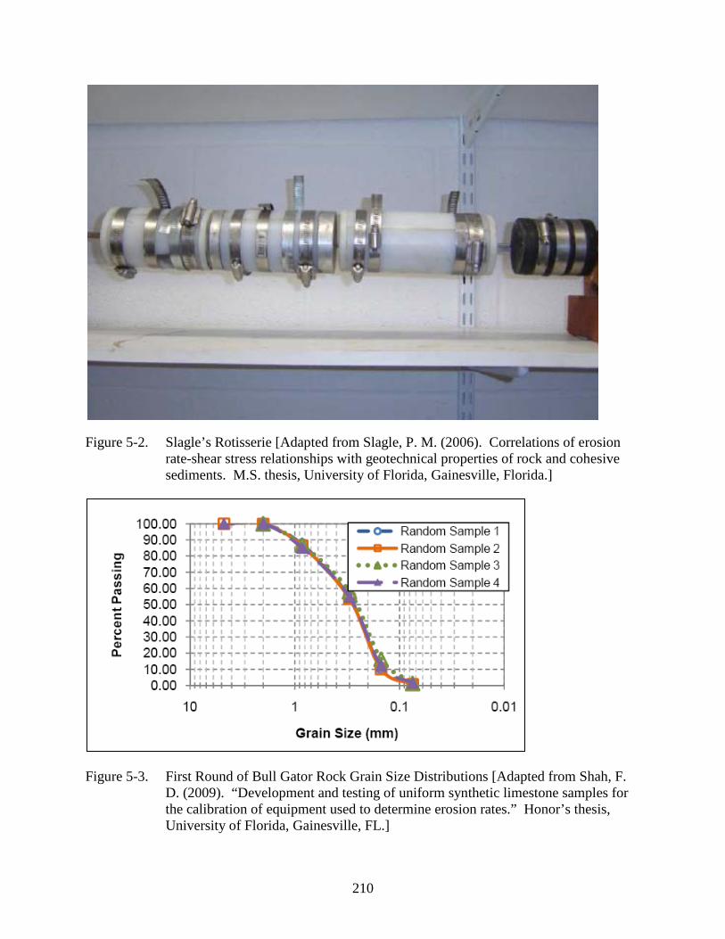
210

Figure 5-2. Slagle’s Rotisserie [Adapted from Slagle, P. M. (2006). Correlations of erosion rate-shear stress relationships with geotechnical properties of rock and cohesive sediments. M.S. thesis, University of Florida, Gainesville, Florida.]

Figure 5-3. First Round of Bull Gator Rock Grain Size Distributions [Adapted from Shah, F. D. (2009). “Development and testing of uniform synthetic limestone samples for the calibration of equipment used to determine erosion rates.” Honor’s thesis, University of Florida, Gainesville, FL.]

211

Figure 5-4. Strength Test Results from First Round of Bull Gator Rock Mixes. The orange line is cohesion; the green line is from compressive strength; the blue line is tensile strength.

Figure 5-5. Batch 1 Bull Gator Rock after RETA 24-hr. RETA Test [Adapted from Shah, F. D. (2009). “Development and testing of uniform synthetic limestone samples for the calibration of equipment used to determine erosion rates.” Honor’s thesis, University of Florida, Gainesville, FL.]

2.5 3 3.5 4 4.5 5 5.5 6 6.5 70

500

1000

1500

2000

2500

3000

3500

4000

W/C Ratio

Stre

ngth

(kP

a)

y(x) = a x n̂ + ca = 5164.4c = 95.343n = -1.9641R = 0.99318 (lin)

y(x) = a x n̂ + ca = 1.3561e+006c = 1483.3n = -6.1676R = 0.98966 (lin)

y(x) = a x + ba = -137.83b = 1009.2R = 0.9735 (lin)

212

Figure 5-6. Batch 2 Bull Gator Rock after RETA 24-hr. Test [Adapted from Shah, F. D. (2009). “Development and testing of uniform synthetic limestone samples for the calibration of equipment used to determine erosion rates.” Honor’s thesis, University of Florida, Gainesville, FL.]

Figure 5-7. Batch 3 Bull Gator Rock after RETA 24-hr. Test [Adapted from Shah, F. D. (2009). “Development and testing of uniform synthetic limestone samples for the calibration of equipment used to determine erosion rates.” Honor’s thesis, University of Florida, Gainesville, FL.]

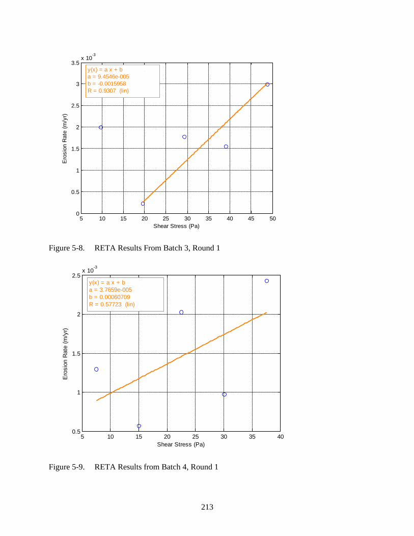
213

Figure 5-8. RETA Results From Batch 3, Round 1

Figure 5-9. RETA Results from Batch 4, Round 1

5 10 15 20 25 30 35 40 45 500

0.5

1

1.5

2

2.5

3

3.5x 10

-3

Shear Stress (Pa)

Ero

sion

Rat

e (m

/yr)

y(x) = a x + ba = 9.4546e-005b = -0.0015958R = 0.9307 (lin)

5 10 15 20 25 30 35 400.5

1

1.5

2

2.5x 10

-3

Shear Stress (Pa)

Ero

sion

Rat

e (m

/yr)

y(x) = a x + ba = 3.7659e-005b = 0.00060709R = 0.57723 (lin)

214


Figure 5-11. Cohesion vs. Erosion Relationship for First Round of Gator Rock Samples

5 10 15 20 25 30 35 40 45 500

0.5

1

1.5

2

2.5

3x 10

-3

Shear Stress (Pa)

Ero

sion

Rat

e (m

/yr)

y(x) = a x + ba = 6.217e-005b = -0.00047792R = 0.78981 (lin)

0 100 200 300 400 500 600 700 8000

0.01

0.02

0.03

0.04

0.05

0.06

0.07

Cohesion (kPa)

Ero

sion

Rat

e (m

/yr.)

10 Pa20 Pa30 Pa40 Pa50 Pa

y(x) = a x n̂a = 2.6343e+008n = -4.1431R = 0.97353 (lin)

y(x) = a x n̂a = 18649n = -2.6386R = 0.98937 (lin)

y(x) = a x n̂a = 7.4657e+010n = -5.1579R = 0.98557 (lin)

y(x) = a x + ba = -1.8911e-006b = 0.002777R = 0.42705 (lin)

y(x) = a x + ba = -1.1824e-007b = 0.0030585R = 1 (lin)

215



5 10 15 20 25 30 35 40 45 50 550

0.02

0.04

0.06

0.08

0.1

0.12

0.14

0.16

Shear Stress (Pa)

Ero

sion

Rat

e (m

/yr)

5 10 15 20 25 30 35 40 45 50 550

0.02

0.04

0.06

0.08

0.1

0.12

0.14

0.16

0.18

0.2

Shear Stress (Pa)

Ero

sion

Rat

e (m

/yr)

216



5 10 15 20 25 30 35 40 450

0.5

1

1.5

2

2.5

3x 10

-3

Shear Stress (Pa)

Ero

sion

Rat

e (m

/yr)

5 10 15 20 25 30 35 40 450

0.2

0.4

0.6

0.8

1

1.2

1.4

1.6

1.8x 10

-3

Shear Stress (Pa)

Ero

sion

Rat

e (m

/yr)

217


Figure 5-17. Gator Rock Test Disc Results

10 15 20 25 30 35 40 45-0.5

0

0.5

1

1.5

2

2.5

3

3.5x 10

-3

Shear Stress (Pa)

Ero

sion

Rat

e (m

/yr)

y(x) = a x + ba = 8.9172e-005b = -0.00098252R = 0.90819 (lin)

218

Figure 5-18. Time Series of Piston Position During Stand Alone SEATEK Test (Data from Batch 1 test at 50 Pa).

Figure 5-19. Zoomed-in Position vs. Time Graph from Batch 1, 50 Pa Data\

0 5 10 15 20 25-1

-0.8

-0.6

-0.4

-0.2

0

0.2

0.4

0.6

0.8

Time (hr)

Pos

ition

(cm

)

7.4 7.5 7.6 7.7 7.8 7.9 8

-0.6

-0.4

-0.2

0

0.2

0.4

0.6

Time (hr)

Pos

ition

(cm

)

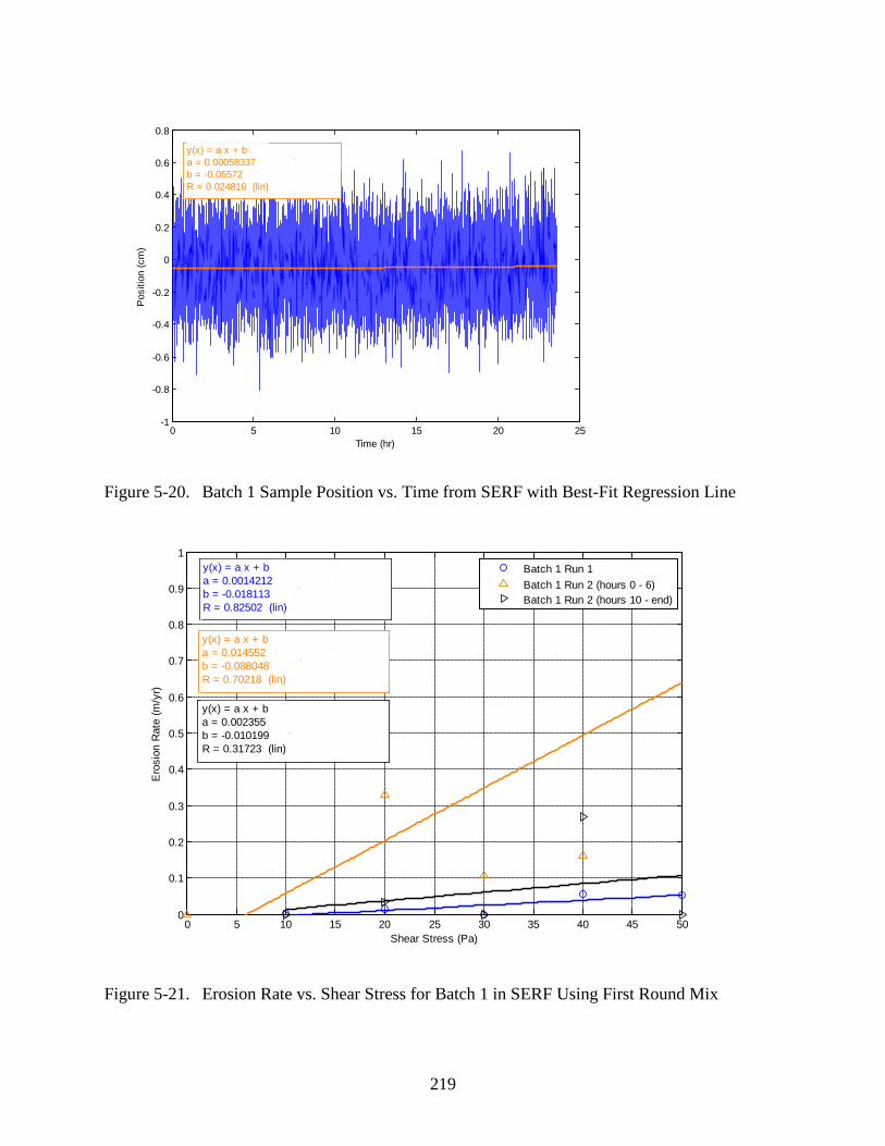
219

Figure 5-20. Batch 1 Sample Position vs. Time from SERF with Best-Fit Regression Line

Figure 5-21. Erosion Rate vs. Shear Stress for Batch 1 in SERF Using First Round Mix

0 5 10 15 20 25-1

-0.8

-0.6

-0.4

-0.2

0

0.2

0.4

0.6

0.8

Time (hr)

Pos

ition

(cm

)y(x) = a x + ba = 0.00058337b = -0.05572R = 0.024816 (lin)

0 5 10 15 20 25 30 35 40 45 500

0.1

0.2

0.3

0.4

0.5

0.6

0.7

0.8

0.9

1

Shear Stress (Pa)

Ero

sion

Rat

e (m

/yr)

Batch 1 Run 1Batch 1 Run 2 (hours 0 - 6)Batch 1 Run 2 (hours 10 - end)

y(x) = a x + ba = 0.0014212b = -0.018113R = 0.82502 (lin)

y(x) = a x + ba = 0.014552b = -0.088048R = 0.70218 (lin)

y(x) = a x + ba = 0.002355b = -0.010199R = 0.31723 (lin)

220

Figure 5-22. Erosion Rate vs. Shear Stress for Batch 2 from SERF

Figure 5-23. Erosion Rate vs. Shear Stress for Batch 3 from SERF

10 15 20 25 30 35 40 45 500

0.5

1

1.5

2

2.5

3

3.5x 10

-3

Shear Stress (Pa)

Ero

sion

Rat

e (m

/yr)

10 15 20 25 30 35 40 45 500

1

2

3

4

5

6

7x 10

-3

Shear Stress (Pa)

Ero

sion

Rat

e (m

/yr)

221

Figure 5-24. Grain Size Analysis for Round 2 Gator Rock Mix

Figure 5-25. Non-Dimensionalized Water Retained vs. Strength (WR is the weight of retained water after saturation; WD is the dry sample weight).

0

10

20

30

40

50

60

70

80

90

100

0.010.1110

Perc

ent P

assi

ng

Grain Size (mm)

Round One Gator Rock Mix Round 2 Gator Rock Mix

0.08 0.09 0.1 0.11 0.12 0.13 0.14 0.15 0.160

200

400

600

800

1000

1200

1400

Wr/Wd

Stre

ngth

(kP

a)

Compressive StrengthTensile Strength

y(x) = a x + ba = -953.8b = 303R = 0.57464 (lin)

y(x) = a x + ba = -8993.2b = 2091.4R = 0.83405 (lin)

222

Figure 5-26. Batch A RETA Results

Figure 5-27. Batch B RETA Results

6 8 10 12 14 16 18 20 22 24 260

0.005

0.01

0.015

0.02

0.025

0.03

0.035

0.04

0.045

Shear Stress (Pa)

Ero

sion

Rat

e (m

/yr)

Sample A-1Sample A-2

6 8 10 12 14 16 18 20 22 24 260

0.005

0.01

0.015

0.02

0.025

0.03

0.035

Shear Stress (Pa)

Ero

sion

Rat

e (m

/yr)

Sample B-1Sample B-2

223

CHAPTER 6 VERIFICATION OF THE ROTATING EROSION TESTING APPARATUS (RETA) AND USING RETA RESULTS TO PREDICT EROSION RATES AND SHEAR STRESSES OF

ERODING BED MATERIALS USING COHESION


In an effort to verify results from the Rotating Erosion Test Apparatus (RETA), a semi-

analytical approach was used. Results from the RETA were filtered so that only data that

exhibited a direct erosion rate vs. shear stress relationship was considered. Then, this dataset

was fit to a shear stress deficit erosion rate formula. Results showed agreement between the

formula and RETA results. Dimensional analysis was used to develop relationships for erosion

rate constant and critical shear stress based on other geotechnical parameters. Based on Mohr’s

Circle reasoning, a cohesion term was added to non-dimensional parameters. Cohesion-based

non-dimensional correlations were used to estimate erosion rate vs. shear stress curves and

compared with RETA results. Data showed agreement between the empirical formulae and

actual results, although the R2 value when comparing these two parameters was low. Because

the cohesive dataset was limited, it is thought that this is what led to these low R2 values.


Development of an extensive RETA dataset is labor intensive. The same is true for a

SERF dataset or any dataset in a flume-style device. Even if a comprehensive dataset could be

generated for both instruments, there is no way to verify that the material tested in both machines

is the same from one test to another. The first version of Bull Gator Rock was the most uniform,

regular, and homogeneous manmade material found to date that would stand up to testing in both

devices, and even Gator Rock tests in the RETA showed variability. Although the RETA’s

dataset was quite limited, for a comparison to be made between the RETA and the SERF, the

testing material’s results should be repeatable even with a small dataset. Faced with these

224

difficulties for making a direct comparison between the RETA the SERF, another method was

investigated to determine whether or not the RETA was providing accurate erosion rate and

shear stress relationships.

Since its inception, the SERF has been used limitedly because of issues associated with its

operation. The RETA on the other hand has been used extensively for over five years. The

FDOT SMO has a laboratory with several RETA’s, and these machines are run often with a

variety of soil, rock, and hybrid samples. Every time a test is run its results are added to FDOT’s

comprehensive RETA database. As of 2010, FDOT had conducted RETA testing on 83 different

materials. Materials from both Florida and from out of state were tested. Some materials were

manmade, while other materials were natural. During the SMO tests, at least three shear stresses

were run during each test. Each test lasted for 72 hours. This database represents 6,000 hours of

RETA testing, and it is the most extensive rotating erosion rate testing device database known to

exist. It took years to generate this database, and it would take several more years to generate

anything similar.

As it is set up, the RETA is designed to measure erosion rates and corresponding shear

stress for particle-like erosion only. As discussed at several points throughout this dissertation,

particle-like erosion assumes that a gentle pull or tug removes a few outside particles from a

sediment sample. This pull or tug is different than rock-like erosion in that during rock-like

erosion, a pulsating impulse force removes chunks or blocks of material from the sediment

sample. The overall goal of this project is to use erosion rate testing devices to measure the

sediment transport function that is used in computing scour depth. Recall from Chapter 2 and

Chapter 3 that particle-like erosion is generally defined by functions taking the following form:

( )τfCE ⋅= (6-1)

225

where E is the erosion rate, C is an erosion rate constant, and f(τ) is a function of shear stress.

Although more complicated computations for this function have been presented (for example

Van Prooijen and Winterwerp 2008), they can be approximated by this generalized equation.

Typically, following shields, the shear stress function is instead expressed as a deficit between

bed shear stress and critical shear stress:

( )cbME ττ −⋅= (6-2)

where τb is the bed shear stress and M is the material specific erosion rate constant.

As discussed in Chapter 2, Equation 6.6-16 was discovered in the 1970’s for particle-like

cohesive erosion rates by Kandiah (1974) and Ariathurai (1974). This equation confirmed

analytical results from Einstein (1950), Partheniades (1965), and others. Equations of this form

have been shown to work using a variety of erosion rate testing equipment. For example,

Partheniades verified his equation for erosion rate by measuring sediment concentrations.

Kandiah on the other hand used a device similar to the RETA to develop his expression. In

general, equations similar to Equation 6.6-17 have shown global relevancy for the particle-like

cohesive erosion problem.

If an equation of this form is valid and the RETA is measuring erosion rate vs. shear stress

relationships correctly, RETA data should fit this form as well. Although a direct comparison

between the RETA and the SERF proved difficult, a direct comparison between the RETA and

equations of this form is possible because of the existence of the RETA database. The technique

used for this analysis was to take the RETA database and try to fit data from it to Equation 6.6-2.

This meant that instead of just comparing the RETA to one other dataset using one other erosion

rate testing device, the RETA is compared with every other cohesive erosion study.

226

6.3 RETA Verification

The first step of RETA data analysis was to filter the RETA dataset so that only particle-

like results were analyzed. For each material in the RETA database, erosion rate and shear stress

were plotted against one another, and best-fit least squares regression line was fit to the data

points. If the line had a positive slope (Figure 6-2), the material for which the curve was

generated was used for overall analysis; if the line had a negative slope (or no slope), the

material was ignored and rock-like erosion conditions were presumed to have dominated that

particular RETA test (Figure 6-1).

Filtering cut the number of samples used for analysis. Whereas the dataset started with

plots relating erosion rate to shear stress for 83 materials, after filtering, only 32 materials fit the

stringent erosion rate-shear stress curve criteria (approximately 40%). Although this looks like a

great deal of data elimination, for a material to survive a RETA test, it must be resilient.

Generally resilient materials are harder and stiffer than materials that crumble under the moment

forcing associated with RETA testing. In other words materials that are able to withstand a

RETA test are more rock-like, which implies that they are more likely to respond to erosion via a

rock-like mechanism. In this context then, a 40% data recovery rate is actually quite precise.

Once filtering was completed, a brief analysis was conducted to compare average rock-like

erosion quantities with implied particle-like erosion quantities. In general, materials that exhibit

direct shear stress to erosion rate relationship erode an order of magnitude faster than materials

that do not exhibit a direct shear stress to erosion rate relationship. This fits with the overall

rock-like erosion argument.

Once filtering had been completed, the next step in fitting a shear stress deficit equation to

the RETA dataset was to find the critical shear stresses associated with each material. By

definition, erosion rate below the critical shear stress point should equal zero. Therefore, the

227

critical shear stress should be defined as the x-intercept corresponding to a material’s erosion rate

vs. shear stress line. For each case where a direct erosion rate vs. shear stress relationship was

observed, the critical shear stresses were estimated using the corresponding best-fit least squares

regression equation. Bed shear stress and erosion rate were measured directly during each

RETA test. With critical shear stress estimated from the best-fit regression lines, the only

unknown in Equation 6-1 was M, the erosion rate constant. For each erosion rate and shear

stress point, the value of M was computed.

As a basis of comparison with the Equation 6.6-2 linear erosion approximation, the most

recent analytical expression for erosion rate was also used (Van Prooijen and Winterwerp 2008).

Van Prooijen explains that his expression for erosion rate can be approximated using a three-

piece function that also utilizes a shear-stress deficit approach and an erosion rate constant.

Erosion rate constant was also computed using Van Prooijen and Winterwerp’s set of equations.

>

−

+

−

+

−

<

=

7.1 if 1

204.0823.0904.0144.0

52.0 if 0

23

c

b

c

b

c

b

c

b

c

b

c

b

cME

ττ

ττ

ττ

ττ

ττ

ττ

τ

(6-3)

These two approaches for solving for M differ only slightly – only by 0.984%. Results were

non-dimensionalized, and a best-fit regression line was fit through the dataset (Figure 6-3).

Based on Equation 6-1, both the slope and the x-intercept of the regression line should

have been 1.0. As shown, with a high R2 value (0.8279), the slope and the intercept of the

regression line are extremely close to where they should be. The x-intercept shows an error of

0.93% and the slope shows an error of 11.78%. Generally, the Equation 6-1 appears to be a

somewhat conservative estimate of erosion rate. The Van Prooijen and Winterwerp Equation

228

appears to capture true erosion rates at lower shear stresses somewhat better than the linear

approximation – particularly when bed shear stress approaches critical shear stress. Overall,

from this analysis, data from the RETA appears to fit correctly. This implies that when a direct

shear stress vs. erosion rate curve is developed, the RETA is providing accurate results.

6.4 Extending RETA Results – Predicting Erosion Rate as a Function of Material Strength

Based on the relatively small error associated with the preceding analysis, there was

confidence behind RETA results. The next step in this study involved trying to find a way to

correlate erosion rate constant and critical shear stress to another geotechnical property of rock-

like bed materials. The goal of this phase of research was to eliminate or reduce the need for

extensive RETA testing. If the need for RETA tests could be cut down – to a situation where a

user simply had to run a RETA test to confirm or disprove a direct erosion rate vs. shear stress

relationship – this would be invaluable. Based on the Mohr’s Circle analysis in Chapter 2, if

erosion rate is to be a function solely of shear stress, then the y-intercept of the Mohr’s Circle

failure line, or cohesion, should be correlated to erosion rate. This Section discusses attempts to

use cohesion to approximate a material’s erosion rate constant and critical shear stress.

6.4.1 Approximation of M

The first goal was to approximate M as a function of a bulk material property. Intuitively,

as material gains strength, erosion rate should decrease. Likewise, as the material gains strength,

its critical shear stress should increase, and therefore overall, the erosion rate constant, M should

decrease. A correlation was developed between erosion constant, M and material cohesion, or C

(Figure 6-4). As shown, there appears to be a relatively strong correlation between these two

parameters. Previously, for clay-like materials, attempts have been made to correlate M to

critical shear stress, but for the materials tested in the RETA, no direct relationships could be

computed between critical shear stress, erosion rate constant, or material strength (Figure 6-5).

229

The relationship given in Figure 6-4 for M was compared with computed M values from

erosion rate data. Although in Figure 6-4, the relationship between M and cohesion appears to be

excellent, when comparing the equation from Figure 6-4’s trend line with measured data (Figure

6-6), results start to deviate. Using the predictive equation shown in Figure 6-4, the R value

between Mmeasured and Mcalculated drops from 0.92 to 0.69 although even with this lower R value,

the equation of the line is nearly where it should be (along y=x, Figure 6-6). If the relationship

developed in Figure 6-4 is used to predict erosion rate and compared with measured data, results

are still reasonable, even though M appears sensitive to cohesion (Figure 6-7). The best-fit line

plotted for measured vs. predicted values of erosion rate lies within 10% of where it should be

(along y = x). The magnitudes of measured erosion rate vs. predicted erosion rate are excellent,

although the predicted erosion rate is on average lower than the measured value. Still, overall,

when dealing with erosion rates on the order of magnitude of mm/year, this analysis should

provide the correct order of magnitude for erosion.

6.4.2 Dimensional Analysis

Because it looked as though it was possible to predict M from material strength, the next

step was to non-dimensionalize this parameter. Based on dimensional analysis, it was

hypothesized that erosion rate constant should be non-dimensionally depended on the ratio

between material strength and critical shear stress such that:

=

Cf

uMC cτ

*

(6-4)

In this expression, C is cohesion, τc is critical shear stress, M has been converted to m2s/kg by

dividing by material density, and u* is the friction velocity associated with the critical shear

stress such that:

230

ρτ cu =* (6-5)

According to this argument then, as the ratio between material strength and critical shear

stress increases, erosion rate constant should decrease. Intuitively, this appears to fit what

Gordon’s 1991 memo already stated – stronger materials tend to erode less quickly than weaker

ones (Figure 6-8). The R value for this relationship is 0.86. More data is needed to shore up this

relationship between material strength and erosion rate constant. This is emphasized when one

uses the logarithmic expression in Figure 6-8 to estimate erosion rate directly. In contrast to

Figure 6-7, erosion rate is not as accurate as it was when using the dimensional relationship

between material strength and erosion rate constant (Figure 6-9). As shown, the R value drops to

0.86 when the non-dimensional expression is used, and the best-fit line through the data points

under predicts the erosion rate by approximately 30% on average. As before, the same order of

magnitude is recovered.

6.4.3 Approximating τc

With a correlation developed between material strength and cohesion, the only remaining

unknown in the Equation 6.6-2 (and the non-dimensionalized cohesion relationship) was critical

shear stress. Development of a relationship between material strength and critical shear stress

has been done before for clay-like particles. Migniot (1986) developed an expression that

showed a relationship between upper Bingham yield stress and critical shear stress such that:

≤>

= Pa 6.1 ;289.0Pa 6.1 256.0

y

y

ττττ

τy

yc (6-6)

Migniot was dealing with much softer and weaker sediments than the sediments found in

the RETA database. Migniot’s critical shear stresses were four orders of magnitude higher than

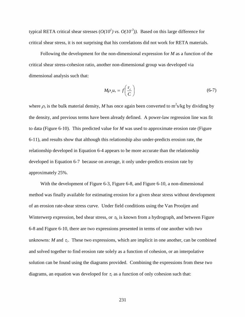
231

typical RETA critical shear stresses (O(101) vs. O(10-3)). Based on this large difference for

critical shear stress, it is not surprising that his correlations did not work for RETA materials.

Following the development for the non-dimensional expression for M as a function of the

critical shear stress-cohesion ratio, another non-dimensional group was developed via

dimensional analysis such that:

=

CfuM c

sτρ * (6-7)

where ρs is the bulk material density, M has once again been converted to m2s/kg by dividing by

the density, and previous terms have been already defined. A power-law regression line was fit

to data (Figure 6-10). This predicted value for M was used to approximate erosion rate (Figure

6-11), and results show that although this relationship also under-predicts erosion rate, the

relationship developed in Equation 6-4 appears to be more accurate than the relationship

developed in Equation 6-7 because on average, it only under-predicts erosion rate by

approximately 25%.

With the development of Figure 6-3, Figure 6-8, and Figure 6-10, a non-dimensional

method was finally available for estimating erosion for a given shear stress without development

of an erosion rate-shear stress curve. Under field conditions using the Van Prooijen and

Winterwerp expression, bed shear stress, or τb, is known from a hydrograph, and between Figure

6-8 and Figure 6-10, there are two expressions presented in terms of one another with two

unknowns: M and τc. These two expressions, which are implicit in one another, can be combined

and solved together to find erosion rate solely as a function of cohesion, or an interpolative

solution can be found using the diagrams provided. Combining the expressions from these two

diagrams, an equation was developed for τc as a function of only cohesion such that:

232

+=

b

Ca

Cu

CuA c

kc

s

ττρ

ln*

*

(6-8)

where A = 2.17x10-7, a = -8.29x10-6, b = -7.12x10-5, and k = 0.545. Solving this equation for τc

and comparing with measured values for τc led to development of Figure 6-12.

The errors associated with the best-fit curves from the two non-dimensional groups appear

to have compounded leading to a large error between actual and estimated critical shear stress

estimates. This was expected since the sum of the errors of the two non-dimensional groups was

on the order of 60%. Using the predicted values for critical shear stress, new values of M were

computed, and they in turn were used with the computed critical shear stresses to solve for

erosion rate (Figure 6-13).

6.5 Discussion and Future Work

The most significant result from this study is that data from the RETA database has been

shown to fit a shear stress deficit equation. Several assumptions with the cohesion estimating

method have been alluded to, but should be discussed explicitly. As shown in most of the

cohesion plots, only eight cohesion data points are shown. Until 2006, no one had realized that

cohesion could possibly be related to erosion rate. When RETA tests were conducted then, a

separate cohesion test was not conducted on material before ‘06. As a result, the number of

cohesion points is limited. Combine the time-frame limits with initial filtering requirements, and

the cohesion dataset is small compared with the overall usable RETA dataset. More research

needs to be done to determine whether or not the correlations developed in Section 6.4 hold up

when more data points are used to develop these curves.

The fundamental assumption in using cohesion as a correlating parameter with the RETA

dataset is that the materials on which cohesion was measured are similar to the materials on

which erosion was measured. Quantifying a material’s erosion rate vs. shear stress relationship

233

and a material’s cohesion value requires three sediment samples. During each test – tensile

strength, compressive strength, and RETA – the sediment sample is destroyed. Using cohesion

as the correlating factor assumes that unlike the Round 2 Bull Gator Rock samples, there is little

variability among the three sediment cores. This assumption may or may not be true; a method

for verifying sample uniformity should be developed if a method similar to this is to be used for

design.

If the dataset used to construct these correlations can be extended though, and if uniformity

between samples can be established, results from this study are promising – especially when

examining Figure 6.4.10. Although the R value (which again is probably caused by a lack of

data points) is poor (0.764), the slope of the best-fit line through the dataset is within 5.5% of

where it should be. This indicates that, this method for predicting erosion rate based only on

material strength has the potential to provide an accurate estimate of actual erosion rate. If the

data set becomes more populated, more accurate critical shear stress estimates and more accurate

erosion rate constant estimates would follow.

This method does predict the order of magnitude of erosion properly. On average, it also

provides a slightly conservative estimate of erosion rate. Although the % error between this

method and the actual erosion rate is relatively high, in terms of actual magnitudes of erosion

rates, it is fairly low. On average, this method for predicting erosion rate over predicts erosion

by 0.52 mm per year; the maximum error is 3.86 mm of erosion per year; and the minimum error

is an under prediction of 1.28 mm of erosion per year. Although not perfect (as evidenced by the

lower R value in Figure 6.4.10), this method will provide erosion rates with 5 mm of the actual

conditions, and it can potentially lead to a reduction in the amount of SERF or RETA tests. If

234

this method is to be used, a safety factor should be employed because of the uncertainty among

the non-dimensional material strength relationships.

This method may be able to reduce the number of RETA testing. Even though this method

was created using filtered data that represented a direct erosion rate vs. shear stress relationship,

it was also found that data that did not exhibit a direct relationship was an order of magnitude

higher than data that did exhibit a direct relationship. If then, this method is used and it turns out

that the material in question exhibits an indirect erosion rate vs. shear stress relationship or no

shear stress vs. erosion rate relationship, it can be inferred that it must erode less than it would if

it were to obey a direct distribution. Using cohesion to estimate erosion rate would be

considered conservative. However, substantially more data are required to validate this theory.


A summary of work and a list of conclusions are presented below:

1. FDOT’s RETA database was filtered so that only direct erosion rate vs. shear stress relationship data was considered.

2. Filtered data was used in development of erosion rate vs. shear stress best-fit regression lines. Regression lines were used to imply critical shear stress for the eroding material.

3. Implied critical shear stresses were used with erosion rate and actual shear stress data to solve for erosion rate constant.

4. Results were non-dimensionalized and plotted. RETA data showed excellent agreement with shear stress deficit analytical formulas.

5. Cohesion was used to develop two non-dimensional groups to estimate erosion rate constant and critical shear stress.

6. Using cohesion as a predictive erosion parameter shows some promise, although the cohesion dataset for RETA samples is quite limited.

7. More research should be conducted before any of these curves are used for design purposes. Specifically, the erosion rate vs. shear stress vs. cohesion database should be expanded.

235

Figure 6-1. Example of a RETA Material with Rock-Like Erosion Properties

Figure 6-2. Example of a RETA Material with Particle-Like Erosion Properties

0 10 20 30 40 50 60 700

0.001

0.002

0.003

0.004

0.005

0.006

0.007

0.008

0.009

0.01

Shear Stress (Pa)

Ero

sion

Rat

e (m

/yr)

y(x) = a x + ba = -2.1795e-005b = 0.0020288R = 0.86548 (lin)

0 10 20 30 40 50 60 700

0.002

0.004

0.006

0.008

0.01

0.012

0.014

0.016

0.018

0.02

Shear Stress (Pa)

Ero

sion

Rat

e (m

/yr)

y(x) = a x + ba = 0.00039548b = -0.013047R = 0.85269 (lin)

236

Figure 6-3. Non-Dimensional Erosion Results from RETA Data Set

Figure 6-4. Relationship between Erosion Rate Constant and Cohesion

0 0.5 1 1.5 2 2.5 3 3.5 4 4.50

0.5

1

1.5

2

2.5

3

taub/tauc

E/(M

*tau

c)

Data Points Using M from Ariathurai EquationData Points Using M from Van Prooijen EquationAriathurai EquationVan Prooijen Equation

y(x) = a x + ba = 0.9844b = -1.0188R = 0.90323 (lin)

0 500 1000 1500 2000 2500 3000 3500 40000

0.1

0.2

0.3

0.4

0.5

0.6

0.7

0.8

0.9

1x 10

-5

C (kPa)

M (g

/(N-s

))

y(x) = a x n̂a = 0.0060567n = -1.0402R = 0.91887 (lin)

237

Figure 6-5. Relationship between Critical Shear Stress and Erosion Rate Constant

Figure 6-6. M from Cohesion based equation vs. M from Measured Data

0 10 20 30 40 50 600

0.2

0.4

0.6

0.8

1

1.2x 10

-5

tauc (Pa)

M (g

/(N-s

))

0 1 2 3 4 5 6 7 8

x 10-6

0

1

2

3

4

5

6

7

8x 10

-6

M from Data (g/(N-s))

M C

alcu

late

d (g

/(N-s

))

Datay=x

y(x) = a xa = 0.91425R = 0.68863 (lin)

238

Figure 6-7. Predicted Erosion Rate vs. Measured Erosion Rate Using M Based on Material Strength

Figure 6-8. Non-Dimensional Erosion Constant vs. Non-Dimensional Material Strength

0 1 2 3 4 5 6

x 10-3

0

1

2

3

4

5

6x 10

-3

E Measured (m/yr)

E C

ompu

ted

(m/y

r)

Datay=x

y(x) = a xa = 0.88059R = 0.85327 (lin)

10-6

10-5

10-4

10-5

tauc/C

MC

/u*

Data

y(x) = a log(x) + ba = -8.2903e-006b = -7.1191e-005R = 0.85549 (log)

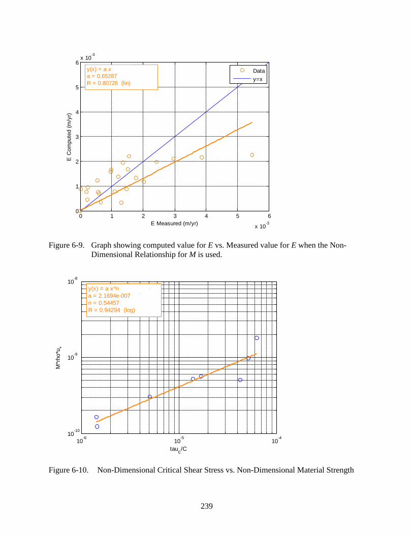
239

Figure 6-9. Graph showing computed value for E vs. Measured value for E when the Non-Dimensional Relationship for M is used.

Figure 6-10. Non-Dimensional Critical Shear Stress vs. Non-Dimensional Material Strength

0 1 2 3 4 5 6

x 10-3

0

1

2

3

4

5

6x 10

-3

E Measured (m/yr)

E C

ompu

ted

(m/y

r)

Datay=x

y(x) = a xa = 0.65287R = 0.80726 (lin)

10-6

10-5

10-4

10-10

10-9

10-8

tauc/C

M*r

ho*u

*

y(x) = a x n̂a = 2.1694e-007n = 0.54457R = 0.94294 (log)

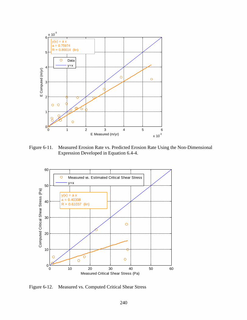
240

Figure 6-11. Measured Erosion Rate vs. Predicted Erosion Rate Using the Non-Dimensional Expression Developed in Equation 6.4-4.

Figure 6-12. Measured vs. Computed Critical Shear Stress

0 1 2 3 4 5 6

x 10-3

0

1

2

3

4

5

6x 10

-3

E Measured (m/yr)

E C

ompu

ted

(m/y

r)

Datay=x

y(x) = a xa = 0.75974R = 0.86614 (lin)

0 10 20 30 40 50 600

10

20

30

40

50

60

Measured Critical Shear Stress (Pa)

Com

pute

d C

ritic

al S

hear

Stre

ss (P

a)

Measured vs. Estimated Critical Shear Stressy=x

y(x) = a xa = 0.40308R = 0.61037 (lin)

241

Figure 6-13. Predicted Erosion Rate Using Cohesion Computation vs. Actual Erosion Rate

0 1 2 3 4 5 6

x 10-3

0

1

2

3

4

5

6x 10

-3

E Measured (m/yr)

E C

ompu

ted

(m/y

r)

Datay=x

y(x) = a xa = 1.0458R = 0.76412 (lin)

242

CHAPTER 7 A STUDY OF EROSION RATES, SHEAR STRESSES AND DENSITY VARIATIONS OF

SAND/CLAY MIXTURES


In an effort to generalize sediment transport functions for sand-clay mixtures, a series of

tests was conducted in the Sediment Erosion Rate Flume (SERF). Results from the tests show

that shear stress on sand-clay mixtures corresponds to roughness such that as roughness (average

sediment diameter) increases, shear stress increases. Work in this study provides some data for

the question of suspended particle effects on shear stress. This study showed that for a smooth

wall, as suspended particle concentration increases, shear stress does not necessarily

correspondingly increase. Erosion rate testing was inconclusive. Generally, erosion rate testing

showed that sand-clay mixtures’ erosion response is sensitive to how the sand-clay mixtures are

initially created. Changes in initial water content and compaction methods affect erosion rate as

much as or more so than sand-clay ratio. More research, particularly on natural samples, is

needed to generalize the erosive behavior of sand-clay mixtures.

7.2 Review of Relevant Background and Motivation for Research

As discussed in Chapter 2, the EFA-SRICOS method for predicting scour depth presumes

that a relationship exists between erosion rate and shear stress for an eroding bed material. Some

particle-like erosion models have been proposed over the years for cohesive bed materials.

(Einstein 1950, Mehta and Lee 1992, Van Prooijen and Winterwerp 2008, etc.). Most of these

erosion models presume a uniform sediment diameter. Some models have been developed for

determining the critical shear stress of cohesive bed materials that are composed of mixed

elements (Barry 2003, Sharif 2002), but sediment transport models for mixed-bed sediments

have yet to be developed. If a direct erosion rate vs. shear stress relationship exists for mixed

bed materials, then it may be possible to determine critical shear stress and use a particle-like

243

stochastic erosion model. If a direct erosion rate vs. shear stress relationship does not exist for

these materials however, application of a particle-like erosion model may be inappropriate.

The Rotating Erosion Test Apparatus (RETA) database described in Chapter 6 was

obtained by running tests on materials that conform to the stringent guidelines associated with

RETA testing. For a material to be tested in the RETA, it must erode nearly uniformly from top-

to-bottom, it must be strong enough to stand up on its own, and it must be strong enough to

withstand the forces associated with the RETA’s spinning annulus. Generally speaking,

materials that meet these requirements are stiff, hard, strong, rock-like earth materials. The Bull

Gator Rock described in Chapter 5 was engineered to mimic the characteristics of hard, stiff,

strong, rock-like materials that constitute successful RETA tests.

The distinction between rock-like cohesive sediments and weaker cohesive sediments is

important. RETA database analysis showed a split between rock-like and particle-like erosive

behavior for samples that are strong enough to withstand a test. For weaker cohesive bed

material such as sand-clay mixtures, there is limited available data.

The goals then of this phase of research are then two-fold. First, is to determine how

mixed-bed earth materials behave. Do they obey a direct erosion rate vs. shear stress

relationship or do they exhibit more rock-like erosion qualities? If mixed-bed earth materials

respond to a direct erosion vs. shear stress pattern, is it possible to generalize this behavior? For

example, may it be possible to claim that an increase in clay content decreases the erosion rate?

Barry and Sharif indicate that varying clay contents in a sand-clay mixture affect critical shear

stress, so it may be possible that varying clay contents also affects erosion rate.

7.3 Materials and Procedure

The Sediment Erosion Rate Flume (SERF) was used exclusively to obtain erosion rates

and shear stresses for a range of sand-clay mixtures. Although originally the plan was to conduct

244

tests at 12.5% clay intervals from 0% clay to 100% clay, unexpected testing results forced

investigators to limit to the SERF dataset to 0% clay, 25% clay, 50% clay, 75% clay, and 100%

clay.

7.3.1 Materials

Edgar Plastic Kaolinite (EPK) and industrial sand were obtained from Edgar Minerals, Inc.

of Edgar, FL. Grain size distributions for these materials were obtained (Figure 7-1 and Figure

7-2).

7.3.2 Shear Stresses

Shear stresses needed to be determined for the bed materials to be used during the test.

Recall from Chapter 4 that shears stress is dependent on roughness. Because of this, a similar

series of shear stress tests was conducted on sand-clay mixtures using the shear stress sensor.

Sensor discs were prepared at 12.5% clay increments from 0% clay to 100% clay so that a

relationship between flow speed and sample roughness could be determined. This 12.5%

distribution corresponds to the original testing plan.

Two different test-disc preparation procedures were used during shear stress testing. The

first round of disc-preparation used the method described in Chapter 4. Sand and clay were

weighed in the appropriate proportions and mixed as dry materials in a small Tupperware

container. Plastic test discs were coated with JB Weld epoxy. Then, the sand-clay mixtures

were spread out over a table and the acrylic test discs were pressed onto each of the sand-clay

mixtures. At least three test discs were made for each sand clay mixture to insure that a true

representative roughness was captured from each mixture batch.

When epoxy is spread on the plastic test discs, the goal is to spread it evenly, but despite

best efforts, sometimes small ripples (thickness less than the diameter of the pinhead) will be

formed as the epoxy is spread. When sand content is relatively high, these ripples are masked

245

because the diameter of a sand grain is much larger than the diameter of a ripple. When sand

content is low however, the diameters of clay particles are on the same order of magnitude as the

size of the ripples. As a result, when the clay particles stick to the plastic test disc, small epoxy

ripples are exposed – thereby slightly falsely increasing the test-disc’s roughness. To combat

this issue, a second disc-preparation method was invented. Fiberglas resin was poured into 50

mm molds. Then, the sand-clay mixtures were sprinkled onto the fiberglass before it dried.

Because the planed fiberglass should be self-leveling, it was thought that pouring a sand-clay

mixture onto the fiberglass before it dried would create a ripple-free sample.

This fiberglass method worked well when sand content was high – especially under 100%

sand conditions. Unfortunately, as sand content was reduced and clay content increased, this

method became much less successful. Under higher clay content conditions (anything above

12.5%), the presence of clay particles interfered with the fiberglass hardener. The result was that

the test discs either did not dry properly, or the discs dried at differential rates. When differential

drying occurred, the discs’ edges dried much faster than the discs’ mid-sections so that when the

discs were removed from the molds, some of the mid-section would “stick” to the molds’ top,

and a concave surface was created along the discs’ front-face.

When put into the shear sensor, this concave disc surface could not be fully leveled with

the flume bottom. If the bottom of the concave surface was leveled, the side walls would

protrude into the flume such that when water was run through the flume, the shear sensor would

also measure a normal component of force on the test disc. If the side walls were leveled with

the flume bottom, the bottom would not be level, and the correct shear stress would not be

measured either. Tests were conducted on the discs to see how much of an effect this concave

246

surface had on overall results compared to the effect of epoxy ripples. In either fiberglass resin

tests or epoxy-glued disc tests, testing on each test disc was repeated at least three times.

7.3.3 Mixing Procedure

Because the goal of this study was to determine sand-clay erosion behavior and attempt to

generalize erosion behavior as a function of clay content, samples for testing had to be relatively

uniform and repeatable. There was some question as to how to properly mix sand and clay

together to produce uniform, repeatable samples. Previous research with sand-clay materials is

limited. One reference (Barry 2002) indicates that when he conducted his tests, he made his

samples by “adding tap water and working by hand.” He does not indicate how much tap water,

but he does describe his bulk density after the sample has been prepared.

Rather than use a target density procedure which would be difficult to duplicate, especially

when making a SERF piston-cylinder sample, different procedures were developed. First,

investigators tried to mix sand and clay dry and slowly add water to the samples from the

bottom-up (as with Bull Gator Rock). The result was a soup-like mixture with little apparent

bonding between sand grains and fine sediment. Eventually, investigators realized that if water

was added to the sand-clay mixture as it was mixed, sand and clay began to flocculate. The

obvious question became how much water to add during mixing? Rather than pick an arbitrary

amount of water, investors settled on using an already established parameter – the optimum

water content based on a Proctor Test (Figure 7-3).

Because the 100% sand sample does not have any cohesive material in it, optimum water

content could not be obtained. Because of this, sand mixing procedure was slightly different

from sand-clay mixing procedure. The sand mixing procedure and sand-clay mixing procedure

are given below:

247

7.3.3.1 Sand mixing procedure

The sand mixing procedure is as follows:

1. A SERF piston cylinder was thoroughly cleaned to eliminate contamination from other sand or clay particles. The piston was inserted into the cylinder and its O-rings were thoroughly greased.

2. The weight of the piston-cylinder was recorded.

3. The distance to top of sample was recorded and divided by 4. Then, the cylinder was filled ¼ of the way to its top.

4. A 2.5 lb. compaction hammer was used to deliver 17 blows to the sample. This blow count and hammer weight was based on the compactive effort delivered during Proctor tests. Because the SERF sample is smaller than the sample for a Proctor mold, calculations were developed to ensure that the same compactive effort was used under both conditions.

5. Once the first sample lift had been completed, a 2nd, 3rd, and 4th lift were added to the sample and compacted with the same blow count used in (3).

6. The 4th lift was planed with the sample-cylinder surface.

7. Water was slowly added to the sand-clay sample using a burette, a tube, and a small plastic pipe fitting. Water flow rate was less than 0.1 mL/sec.

8. Once the sample had been fully saturated (as evidenced by water coming out of the top of the sample), the sample was weighed so that its density was known.

7.3.3.2 Sand-clay mixing procedure

The sand-clay mixing procedure is as follows:

1. The volume of the piston-cylinder was computed and multiplied by an assumed worst-case total density of 2.65 g/cm3. This number was multiplied by the percent clay to get the required mass of clay and it was multiplied by percent sand to get the required mass of sand.

2. The appropriate mass of sand and clay were weighed using an electronic balance.

3. Sand and clay were evenly and slowly poured into a mixing bowl and the mixer was turned on “low” for approximately 5 min. Halfway through mixing, the mixer was stopped and the sides of the bowl were scraped so that any material on the sides would be moved toward the center of the bowl.

4. The mixer was turned on again, and half of the water required to achieve optimum water content was measured with a graduated cylinder and added to the mixing bowl.

248

5. Once the mixer had run for two minutes, it was stopped, scraped, and restarted. Then, the ¾ of the remaining water was added to the bowl.

6. After two minutes, the mixer was stopped and scraped again.

7. The mixer was restarted, set to “high,” and the rest of the water was added. The mixer was allowed to blend for another 2 minutes.

8. The sand-clay mixture was added to the piston-cylinder until the piston-cylinder was ¼ full.

9. Using the modified 2.5 lb. Proctor hammer, 17 blows in a circular pattern were applied to the sample.

10. Steps (9) and (10) were repeated for lifts of ½ full and ¾ full. For the final lift, a collar was placed over the tube, and the tube was overfilled such that material extended approximately ¼ above the lip. Again, 17 blows were applied to the sample.

11. A metal screed was used to level the sample with the top of the piston-cylinder.

12. A small piece of remaining material was placed in a water content canister, and the canister was placed in an oven at 125oF so that water content could be measured.

13. The sample was attached to a burette-valve device and filled from the bottom-up so that until it was saturated. Saturation was defined as water flowing out from the top of the sample.

14. The final mass of the sample was recorded.

15. The sample was placed in the SERF.

7.3.4 SERF Testing

The procedure for SERF testing is outlined in Appendix B, but in brief, the following

procedure was used during tests:

1. The sample was loaded into the SERF such that the two 1.0 mm cutouts along the top of the sample cylinder lined up with the lasers.

2. The motor and motor platform were slowly moved into position.

3. The SERF was filled with water.

4. Once the flume had been pressurized, the sample was allowed to slightly protrude into the flume.

5. A high flow rate was used to re-level the sample with the flume’s bottom.

249

6. The flume pumps were started at a low flow rate. Flow speed was incrementally increased until incipient motion was detected.

7. Because tests were run with sand-clay, the lasers needed to be used exclusively during SERF tests. Therefore, the lasers were turned on, and the test began.

8. At the end of the SERF test, once the sample was empty, a new sample was prepared, and steps 1-7 were repeated.

7.3.5 Procedural Variations

In the preceding SERF discussion, Step 7 is intentionally described vaguely. At first, the

plan was to vary flow rates randomly from 0 Pa to a shear stress where erosion rate was

approximately 1.0 mm/s. The 1.0 mm/s erosion rate criterion was chosen because the laser-

motor system cannot keep up with erosion rates higher than this. At each flow rate and shear

stress, erosion rate would be recorded, then the flow rate would be changed, and the procedure

would repeat.

This procedure assumes that a sample will erode uniformly from top-to-bottom. As will be

described in Section 7.4, this did not happen. Instead, erosion rates varied as a function of

sample depth. Because of localized hard patches where bulk density increased, which

corresponded to depths at which the modified Proctor hammer was used, erosion was non-

uniform. To capture this behavior, eventually instead of using several shear stresses on one

sample, one shear stress was tested per sample.

Because of these differential erosion rates, investigators tried to develop samples that

would respond more uniformly. During mixing, water contents were modified so that double the

optimum water content was used to determine if mixed water content affects erosion behavior.

For some clay contents, a third batch of samples were made where the number of lifts during

mixing was reduced from 4 lifts to 2, while the blow count delivered per lift was doubled to

determine if lift height affected sample erosion or uniformity.

250

7.4.6 Density Profile Tests

Because of the differential erosion rates, a series of samples were prepared where density

profiles were measured. To run these tests, the samples were mixed according to the procedure

outlined in Section 7.3.3. Then, samples were extracted from their molds and cut into 1.5 cm

segments using a modified coping saw. Instead of a typical saw blade, the modified coping saw

used a 3-strand braided 28-gauge wire. The sample segments were weighed, dried, and

reweighed to give both dry and wet densities as a function of sample depth. Results were

compared with lift depths recorded during sample preparation.

7.4 Experimental Results and Analysis

Experimental results are divided into three segments:

• Results from shear stress tests • Results from SERF tests • Results from Density Profile Tests

7.4.1 Shear Stress Tests

Shear stress experimental results are divided into results from the epoxy-glued discs

(Figure 7-4 through Figure 7-13) and results from the fiberglass resin discs (Figure 7-14 through

Figure 7-23).

Although Figure 7-23 shows that the 100% clay mixture does indeed have the lowest shear

stress associated with it, this figure also shows that certain sand-clay percentages may produce

higher shear stresses than the shear stresses seen under 100% sand conditions. This may be true

under special circumstances – for example, when floc erosion instead of particle erosion is an

important erosion mode – but as of yet, there is no known way to predict when this will occur

and the purpose of this test was not to predict the floc size that would erode from a sample, but

rather, to find the relative shear stress magnitudes along a sample face resulting from simple

particle effects. Figure 7-23 shows that when clay content is at 87.5% and when clay content is

251

at 62.5%, shear stress is higher than it would be when there is no clay in the sample. Based on a

particle-based roughness rationale, this must be impossible.

These higher shear stress readings then can be attributed to the concave nature of the test-

discs. Because an average leveling height was used even though the disc was not level, the discs

protruded into the flume somewhat (~1 mm – 2 mm). Even this slight protrusion caused a large

increase in the force on the disc because of the added normal component. During the epoxy

testing, the discs were precisely level with the flume bottom, and there were no normal forces

acting on them. Figure 7-23 shows no discernable pattern that would indicate a decrease in

shear stress that corresponds to a decrease in sand content. This appears to contradict the data

shown in Chapter 4 which indicates that as roughness decreases (for a given flow rate), shear

stress should also decrease – especially at higher flow rates.

Because of this, the data in Figure 7-23 must be rejected in favor of the shear stresses

corresponding to the data shown in Figure 7-13. This conclusion has interesting implications

regarding EFA testing because in the EFA procedure, a protrusion of 1 mm into the flume is

specified. This data indicates that shear stresses are sensitive to any protrusion into a flume.

Because the EFA uses a Moody Diagram to estimate shear stresses on its samples (Chapter 4

verified that this was an accurate method), the shear stress should not be underestimated using

this device. But, because a 1 mm protrusion could cause a much higher actual stress on the

sample compared with the stress than would be caused with a level sample, the actual stress on a

sample would be greater because of the normal component. This in turn would produce a higher

erosion rate than usual, and this could lead to an overly-conservative erosion rate-shear stress

curve. For example, the protrusion caused by the wave-like 50 mm test disc under 87.5% clay

conditions shows over a 100% increase in stress at a moderate velocity of 4 m/s. Because

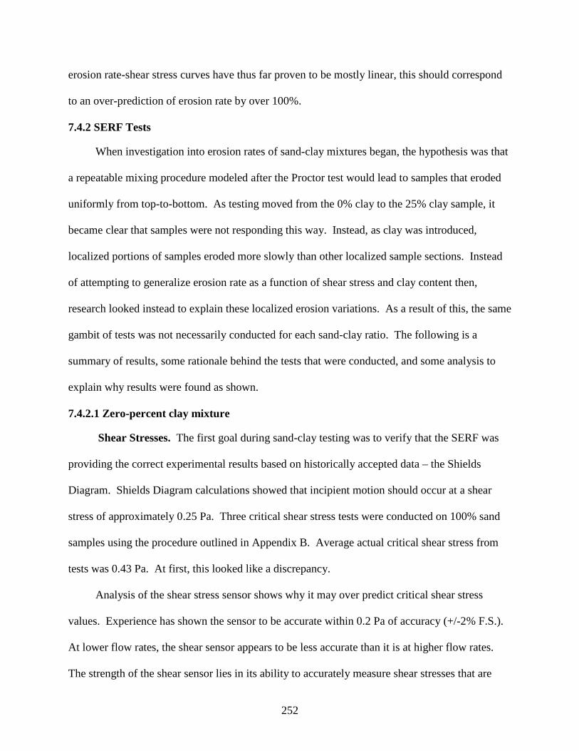
252

erosion rate-shear stress curves have thus far proven to be mostly linear, this should correspond

to an over-prediction of erosion rate by over 100%.

7.4.2 SERF Tests

When investigation into erosion rates of sand-clay mixtures began, the hypothesis was that

a repeatable mixing procedure modeled after the Proctor test would lead to samples that eroded

uniformly from top-to-bottom. As testing moved from the 0% clay to the 25% clay sample, it

became clear that samples were not responding this way. Instead, as clay was introduced,

localized portions of samples eroded more slowly than other localized sample sections. Instead

of attempting to generalize erosion rate as a function of shear stress and clay content then,

research looked instead to explain these localized erosion variations. As a result of this, the same

gambit of tests was not necessarily conducted for each sand-clay ratio. The following is a

summary of results, some rationale behind the tests that were conducted, and some analysis to

explain why results were found as shown.

7.4.2.1 Zero-percent clay mixture

Shear Stresses. The first goal during sand-clay testing was to verify that the SERF was

providing the correct experimental results based on historically accepted data – the Shields

Diagram. Shields Diagram calculations showed that incipient motion should occur at a shear

stress of approximately 0.25 Pa. Three critical shear stress tests were conducted on 100% sand

samples using the procedure outlined in Appendix B. Average actual critical shear stress from

tests was 0.43 Pa. At first, this looked like a discrepancy.

Analysis of the shear stress sensor shows why it may over predict critical shear stress

values. Experience has shown the sensor to be accurate within 0.2 Pa of accuracy (+/-2% F.S.).

At lower flow rates, the shear sensor appears to be less accurate than it is at higher flow rates.

The strength of the shear sensor lies in its ability to accurately measure shear stresses that are

253

still low at much higher flow speeds. In other words, if a creeping flow is moving past the

sensor, it won’t pick up this small deflection in the platform-test disc-leaf spring-Servo magnet

system. This has to do with the mass of these moving parts – which relative to the small flow

speed and the small associated shear stress – is large. Therefore, with the current setup it would

be impossible to with 100% accuracy to measure shear stresses at such a low range. When

dealing with a shear stress less than 1 Pa, accuracy within 2% is actually quite precise.

The next dataset to consider was Trammel’s 2004 data. Here he attempted to verify the

pressure drop system within 5% of accuracy by using a Shields Diagram. Chapter 4 shows that

especially at higher flow rates, the pressure drop method does not accurately estimate shear

stresses in the SERF. Because shear stress can be correlated to a power-law distribution with

respect to velocity, at low flow speeds, the pressure drop readings do converge to a curve that

appears to be the same.

Trammel verified the pressure drop method (again at low speeds) by measuring the

pressure drop on samples that were 1.4 mm, 0.921 mm, 0.696 mm, and 0.508 mm in diameter.

In terms of the tests run during this round of testing, the 0.921 mm data and the 0.508 mm data

are of interest because they should closely correspond to 1.0 mm data and 0.50 mm data

respectively as presented in Chapter 4. Figure 7-24 shows Trammel’s data overlaid with data

from this study. This diagram shows the readings from these two sets of tests are close – on

average within 8.63% of one another. The Shields calculations however are extremely sensitive

to shear stress values; any deviation – even an 8% deviation at such low shear stress magnitudes

– will cause a large deviation in the shear stress entrainment function. This in turn causes a

relatively large difference in the computed shear stress which in turn causes a large deviation in

overall results.

254

Trammel’s collected his pressure readings with a pressure transducer with +/-2.5psi range

at 0.1% F.S. error. This means that Trammel was capturing pressure accurately within +/-

0.0025psi or +/-17.24 Pa. Shear stress is related to pressure drop using the following equation:

( )Lwlplw22 +

∆=τ

(7-1)

In Trammel’s case, he had pressure sensors spaced further apart than the current setup (4

ft. or 1.22 m). If one was to ignore the fact that with this setup most of the flume wall along this

spacing length was smooth and therefore most of the pressure drop was be caused by smooth

rather than rough conditions, the following accuracy calculation would follow:

( )( )( )( ) ( )( ) ( )( )[ ]mmm

mmPaERROR 2032.020445.0222.1

2032.00445.024.17+

±=τ

(7-2)

PaERROR 258.0±=τ (7-3)

This calculation shows that Trammel’s measurements could only have been accurate

within 0.26 Pa – which for some of his measurement shown in Figure 7-24 is less than the shear

stress value than he was measuring. Chapter 4 showed how difficult it is to get accurate readings

from the pressure drop method, and no spectral analysis or filtering of his data except for the

installation of a hard-wired 4th order low-pass Butterworth filter was employed. The fact that

because of his pressure port spacing, most of his pressure drop would have been influenced by

smooth flume bottom and not the roughened sample portion of the flume. On the other hand,

results from the shear stress sensor allowed investigators to conclude that shear stress results

were accurate enough to proceed to erosion rate tests.

Erosion Rates. Based on the preceding analysis, an erosion rate vs. shear stress curve

was developed based on the shear stress vs. flume velocity curve presented in Section 7.4.1

255

(Figure 7-25). Rather than use a simple final position minus initial position divided by time

calculation to find erosion rate (as was used by Trammel and Slagle), a best-fit least squares

regression line was fit to a sample position vs. time plot. Results in Figure 7-25 are developed

from the slopes of these trend lines, and they were non-dimensionalized in the same manner in

which RETA database results were non-dimensionalized in Chapter 6 (Figure 7-26). A 100%

sand sample was allowed to run at a moderate shear stress (3.0 Pa) to verify that erosion rate was

the same from top-to-bottom throughout the sample. Since erosion rate was constant throughout

the sample, 100% erosion data was taken such that multiple shear stresses were used on one

sample. In total, erosion rate tests were conducted on five 100% sand samples.

7.4.2.2 Twenty-five percent clay samples

At first, when the sample mixing procedure presented in Section 7.3.3.2 was introduced, an

additional step was added after Step 16. The sample was put into a bucket for 24 hours to insure

saturation. However, by mistake, one time samples were prepared at the end of the day on a

Friday and tested on a Monday. Over the weekend, it appeared as though consolidation had

taken place, as erosion rates were much smaller than the erosion rates shown in previous tests.

To determine if allowing the samples to sit upright for 24 hours or more played a role in erosion

rate, a sample was prepared and inserted immediately into the SERF. This sample showed a

much higher erosion rate than the erosion rates seen with previous samples that had been allowed

to soak. Because of this then, a standard needed to be developed, and since investigating

consolidation effects is not within the scope of this project, it was decided that zero consolidation

would be used as the standard for future testing. In other words, for samples with clay, samples

would be prepared and immediately put into the SERF.

The 25% sand-clay mixture was the first time that the lasers described in Chapter 3 were

forced to perform sample advancement on their own. Because erosion rates were moderately

256

quick, the issues that were found in using the lasers with the Gator Rock were nearly non-

existent with the clays. The lasers worked as designed. The only downside to the lasers was that

at higher flow rates, the motor could not keep up with the analog blips coming from the lasers.

Therefore, sometimes when erosion rate was high, there would be a backlog of advancement that

should have happened but could not. Once erosion rate leveled out, this would cause sample

penetration into the flume – which in turn would cause the sample to erode even faster and

exacerbate the problem. However, this was only an issue at high flow speeds (relative to the

erosion rate), and if one extrapolates these erosion rates over a year, the result returns kilometers

of erosion per year, which is not possible.

For the 25% clay data run, procedures remained the same as they had for the 0% clay data

run as far as testing the effects of multiple shear stresses per sample. However, during testing,

investigators noticed that with the 25% clay sample, as more of the sample eroded from the

piston-cylinder, the sample appeared to exhibit hard layers. Whenever these hard layers were

encountered, qualitatively it was observed that erosion rate slowed down. Eventually, these hard

layers would erode, albeit through a more undercutting, normal stress induced, rock-like erosion

mechanism, and once the layer had been removed from the sample, erosion would continue on as

normal. Because of this layered effect, at first results were confusing because at first, before the

layered effect was discovered, it appeared as though sometimes lower shear stresses caused

higher erosion rates.

It was evident that the layers probably corresponded to the 4-lifts that were used in sample

preparation by analyzing a time-series of erosion data and allowing the same shear stress to be

run over the entire length of a sample (Figure 7-27). The 4-steps shown in this diagram should

not be a coincidence, especially because this pattern was seen on the 25% clay samples. Of note

257

though is that this 4-step effect is only visible during moderately-paced erosion rates. When

erosion rate is high (Figure 7-28) or erosion rate is low (Figure 7-29), the sample responds much

more uniformly. The interesting thing regarding this pattern is that the best-fit line method for

determining erosion rate, which was an effective indicator of erosion rate beforehand, is not

necessarily relevant under these conditions even though the R2 value is close to 1.0. Figure 7-27

shows two different erosion rates – one slow and one fast.

The slow erosion rate can be explained by the initial portion of a rock-like erosion mode.

During the first part of rock-like erosion, little actual particle movement is seen. Rather, water

flowing past the sample surface serves to weaken the top layer (which can be viewed as a large

chunk of material) by loosening small localized portions of it. Eventually, channels developed

along certain parts of the sample face, and once these channels developed, flow was concentrated

into the sample through them. These channels are analogous to cracks or fractures that form on a

rock face. Eventually, the undercutting flow caused by the channels causes a large chunk of

material (or sometimes most of the sample surface) to erode, and once this happened, the rapid

advancement of the sample into the flume would occur. During rapid advancement, additional

chunks and blocks of material would be removed from the material surface as quickly as the

material advanced. This would continue until another hard layer was exposed. Then, erosion

rate slowed down and the beginning stages of rock-like erosion occurred again. The rapid

sample advancement portion of erosion is similar to a particle-like scenario. The critical shear

stress for this relatively loose, relatively weaker material has already been exceeded, and because

of this rapid erosion of large sections of material is seen. This back-and-forth particle-like vs.

rock-like erosion pattern continued until the sample was gone. In addition to the 3.37 Pa, 13.4

258

Pa, and 40.0 Pa results already presented using the first mixing procedures, experimental results

were obtained at 30.0 Pa and 53.2 Pa (Figure 7-30 and Figure 7-31).

If the hardened layers were caused by the initial stages of rock-like erosion, and the

hardened layers were localized, the conservative solution to the problem should be to eliminate

the hardened sections from the piston position curve and use the rapid advancement portions of

the curve to define an erosion rate. This should give a generalized erosion rate vs. shear stress

relationship. Figure 7-32 was developed by analyzing the flat sections of the five erosion rate

shear vs. shear stress curves. Figure 7-33 was developed by analyzing the rapid advancement

portions of the curves. In both cases, data was cut from the datasets into alternating flat and

rapid advancement sections. Then, a best-fit line was fit to each data string. Since the best-fit

line corresponds to y = mx + b, the average slope coefficient, m was found for each flat case and

each rapid advancement case at each shear stress.

Analysis of Figure 7-32 and Figure 7-33 show that the beginning stage of rock-like erosion

hypothesis appears to be correct. In Figure 7-33, there appears to be strong erosion rate vs. shear

stress relationship for the rapid advancement erosion sections of each of the five samples.

Although there appears to be some relationship between erosion rate and shear stress for the flat

portions of erosion as well, the correlation is not nearly as strong. This corresponds to the notion

that rock-like erosion may have something to do with flow speed, but flow speed is not the only

parameter that affects the normal stresses acting along the sample face. Comparison of these two

figures also confirms what was hypothesized with the RETA database in terms of rock-like vs.

particle-like orders of magnitude. Recall from the RETA database that generally, materials that

did not respond to a direct erosion rate vs. shear stress relationship had erosion rates that were an

259

order of magnitude lower than materials that did have a direct relationship between erosion rate

and shear stress.

The question then became, how does one define the “correct” erosion rate? Should the

erosion rate be defined conservatively by the rapid erosion portions of the signal, or is the

hardened layer portion of erosion more valid? Or, are both of these erosion rate measurements

bad estimates because of the way in which the sample was prepared?

According to a Westergard soil stress distribution, some sand-clay mixtures are assumed to

be comprised of an infinite number of alternating layers of sandy soil and fine grained soil. In

soils such as these, a vertical surface load leads to a lower vertical stress within the soil column

than the stresses that would be seen using a Boussinesq approximation which assumes a uniform

material. Presumably these materials should also exhibit differential erosion rates as observed in

Figure 7-27. However, investigators had to verify that the 4-layers erosion sequence did indeed

respond to the sample preparation method. To do this, a test was run at 13.4 Pa where the

sample was prepared using two lifts (Figure 7-34). Results appear to indicate that sample-

preparation procedure is the same for the differential erosion rate behavior.

After observing this behavior a hypothesis was made that lift-to-lift cohesive forces would

be stronger if the top of the first lift is rougher. Essentially what was happening using an optimal

water content approach was that doing this was like trying to glue two flat, slick, and smooth

surfaces together using relatively small cohesive forces. Instead, what should have happened if

samples were to be nearly uniform was that the compactive effort applied to the top lift should

have been high enough to cause lift-to-lift particle interaction. This could only be achieved if the

sample was allowed to slump more. In other words, allowing for a more easily deformable

material would induce more particle-to-particle bonding per blow, which in turn would create a

260

more uniformly “sticky” material that although weaker, should exhibit lower erosion qualities.

Note that this notion contradicts the erosion as a function of cohesion theory as discussed in

Chapter 6 because this method says that creating a weaker material will actually provide a lower

average erosion rate due to the increase in vertical cohesive forces within the material matrix.

This does not necessarily mean the discussion in Chapter 6 is incorrect; rather perhaps it only

applies to stiffer materials. When unhardened sand-clay samples are present, another mechanism

may be dominant.

Two more samples were prepared using double the optimum water content, and a time-

series erosion test was run on them (Figure 7-35). As shown, the steps that were easily visible

using the first sample preparation method disappear. However, Figure 7-35 shows that on

average, erosion rates are slower than they would be using the preparation method outlined

originally. Note that the samples that were prepared to create Figure 7-35 were mixed with the

original 4-lift mixing procedure. Development of Figure 7-35 shows that a change in the mixing

water content changes erosion rate. This figure shows that weaker samples can erode more

slowly than stronger samples. This was unexpected.

If Figure 7-33 is a conservative estimate of erosion rate vs. shear stress for a 25% clay

sample when the sample is mixed at the optimum water content, Figure 7-35 shows that the

estimate is only accurate under the special-optimum water content case. An interesting study

would be to determine where the tipping point between the two curves is from a mix-perspective.

In other words, if optimum water content produces a certain particle-like erosion rate, and an

increase in water content produces a slower erosion rate, at what point is erosion rate the

maximum? And, is this maximum valid for any layered sediment? Or, does the amount of

layers in the sediment strata play a role? Could layer thickness preclude the development of a

261

particle-like erosion mode from taking place at all? Another interesting question was at what

clay content does this layered effect become relevant? Although investigation started with the

25% clay sample, it may be possible that below a certain clay threshold, layering no longer has

an effect.

At this point, it was obvious that substantial tests would be required to provide one data

point for a 25% clay mixture. Even if the 25% clay mixture problem could be solved, it does not

necessarily apply to other sand-clay ratios. Because the purpose of this project was to bound the

sand-clay erosion problem, investigation into erosion rates for the 25% sand-clay mixture was

stopped. The above analysis shows that a variety of erosion behaviors can be engineered by

varying the initial water contents and lift-heights, but the real question is what do natural earth

materials do? Both the slower layered rock-like erosion and the faster rapid-advancement

particle-like erosion are valid erosion modes.

7.4.2.3 Fifty-percent clay samples

Analysis of the 25% clay samples shows that an increase in the water content may

eliminate the stepping behavior seen under optimum water content mix conditions. When

investigation into the 50% clay samples began, investigators’ first goal was to determine if the

50% sand-clay ratio behaved similarly. As with the 25% mixture, a series of erosion rate tests

was conducted at a variety of shear stresses for the 50% mixture using the initial optimum water

content mix approach (Figure 7-36).

Figure 7-36 shows that the step-like erosion behavior seen for 25% clay mixtures is not as

apparent with the 50% samples. As flow rate (and subsequently shear stress) increases, the step-

like erosion behavior becomes more apparent, but for lower flow rates and shear stresses, step-

like erosion is nearly non-existent. Although perhaps not as obvious from Figure 7-36, when one

262

zooms in on an erosion rate curve at a higher flow rate, the step-like erosion behavior is obvious

(Figure 7-37).

Figure 7-37 also shows another interesting phenomenon. The top layer of each sample

erodes much more quickly than other sample layer (Figure 7-38). As testing time and

subsequently sample depth increases, erosion rates become much slower. This implies that the

bottoms of the 50% samples are more erosion-resistant than the tops of the samples. This

behavior was not seen with the 25% sand-clay mixtures.

Water content was doubled to determine if a change in initial water content would affect

erosion rate behavior. As with the 25% sand-clay mixture, an increase in water content made a

much weaker sample that tended to slump much more easily. This weaker sample showed much

greater resistance to erosion than the optimum water content mixture – so much so that to

observe any erosion, shear stresses had to be increased from the values used for the optimum

water content tests (Figure 7-39).

Figure 7-35 and Figure7-39 show an interesting phenomenon for samples mixed at double

the optimum water content. In Figure 7-39, a ~7 Pa increase in shear stress appears to cause a

high increase in erosion rate. Likewise, Figure 7-35 shows that a 14 Pa increase causes a similar

rise in the magnitude of erosion rate. Beyond this tipping point, erosion rate appears to increase

relatively slowly; below this tipping point erosion rate behaves similarly. This behavior appears

to suggest that for a certain shear stress, erosion rate will transform from a regular slow particle-

like erosion pattern to a more chaotic floc-like erosion scenario.

Visual observation during the erosion rate test showed that the behavior seen below this

tipping point is much different than erosion rate behavior above this tipping point. When erosion

rate is relatively small (as it is at 30 Hz or 35 Hz in Figure 7-39), an observer can see individual

263

flocs breaking from the sample’s surface and moving downstream. Floc erosion is nearly

uniform across the sample face, although the middle of the sample does erode somewhat more

slowly than the sample’s outsides (probably due to where most of the compaction is applied for a

given sample). As erosion rate increases, erosion becomes much more irregular, and an observer

can see large chunks of material removed from the sample. When the flow rate becomes high

enough, erosion transforms to an advanced stage of rock-like erosion. With the 4-lift optimum

water content samples the beginning stages of rock-like erosion were seen – with the hardened

layers and subsequent rapid advancement once the layer was broken. When water content is

doubled, layering does not have as much of an effect, yet beyond a certain point, instead of

steady floc-flow, large-scale chunking is observed.

If samples with higher water contents are more cohesive, this phenomenon appears to

make sense. Whereas for the optimum water content, individual flocs struggle to stick together,

when water content is increased, the cohesive bonds holding flocs together have more of an

effect. This inhibits the creation of hard layers. At the same time, once particle and floc vertical

movement is initiated by the normal forces associated with rock-like erosion this increase in

cohesion causes larger chunks of material to be removed.

Again, the question is how does one define a “proper” erosion rate for any sand-clay

mixture? Once this behavior was observed for the 50% sample, the goal for the 75% sample and

the 100% samples became to bound this “tipping point” between rapid erosion and slow erosion

at higher optimum water contents. Additionally, the original 4-layered mix would be studied to

verify that layering was an important erosion rate effect at certain initial water contents. This is

done with the understanding that until tests are run on a series of natural samples, developing a

generalized erosion rate vs. shear stress relationship for any sand-clay mixtures is premature.

264

7.4.2.4 Seventy-five percent clay mixture

As with the 25% mixture and the 50% mixture, the 75% mixture was studied using a 4-lift

mixing procedure. Both optimum water content and double the optimum water content were

used during mixing. As before, samples were saturated before they were subjected to SERF

testing (Figure 7-40 and Figure 7-41).

The 75% sand-clay mixture shows a tendency that was slight with the 50% sample. As

shown in Figure 7-40, the relationship between sample position vs. time is not linear. The

bottoms of the samples erode much more slowly than the samples’ tops. As such, it would be

inappropriate to fit an erosion rate line to the data. This tendency was shown with the 50%

sample, although this non-linear behavior is much more apparent with the 75% mixture. The

75% sample at optimum water content is similar to the 50% sample at optimum water content in

that the step-like erosion behavior does not exist below a certain shear stress. However, above a

certain flow rate/shear stress threshold, step-like erosion still occurs.

When water content is doubled, the bottom sample layer becomes much harder than the top

sample layers (Figure 7-41). Rapid erosion is seen until this point, and beyond this point erosion

is slow. This bottom layer approximately corresponds to the bottom sample-lift. In other words,

for the first time at any sand-clay ratio, there appears to be some relationship between lift height

and erosion behavior at the higher water content. Below this slow erosion zone, erosion rate is

approximately linear for the higher water content case. Erosion rate cannot be compared with

the lower water content case since erosion at the lower water content is non-linear. Overall, the

75% sample is similar to the other sand-clay mixtures in that erosion is hypersensitive to the

manner in which the sample was prepared.

265

7.4.2.5 One-hundred percent clay

As with the mixtures, two batches of 100% clay were prepared using both the optimum

and double the optimum water contents. By the time testing reached this point, a pattern

emerged. When the water content was doubled, the erosion rate decreased. At the higher water

content, there was a tipping point between regular particle-like erosion and chaotic advanced

rock-like erosion. At the optimum water content, erosion appeared to be step-like and/or non-

linear. Therefore, fitting an erosion rate curve to a sample position vs. time graph is

inappropriate because for a non-linear sample, erosion rate is more dependent on localized

material properties. The 100% clay tests were run simply to confirm this pattern of behavior

(Figure 7-42 and Figure 7-43).

The double optimum water content samples shown here appear to exhibit the pattern from

highly regular particle-like erosion behavior to more chaotic behavior somewhere between 17.76

Pa and 19.41 Pa. Interestingly, the 100% clay sample at optimum water content also appears to

show a tipping point to a more chaotic erosion behavior somewhere between 19.41 Pa and 22.84

Pa. Although this is the case, erosion rate appears to be highly non-linear as it was for the 75%

sample. As more of the sample erodes, the bottom portion of the sample provides more erosion

resistance.

7.4.3 Density Profile Tests

The goal of the density profile tests was to quantify density variability in the sand-clay

mixtures and to compare localized density variations with hardened erosion rates observed

during SERF testing. Results from the density profile tests are presented in Table 7-1 and Figure

7-44 through Figure 7-54. Where appropriate, the black lines represent lift interfaces measured

during sample preparation. Since the most extreme erosion fluctuation with density variability

266

occurred with the 25% sand-clay mixtures (from a stepped-erosion perspective), most density

profiles concentrated on this mixture concentration.

Generally speaking, lift intervals does not necessarily align themselves with localized

density fluctuations. Sometimes a lift interface will line up with a higher density, while other

times it will align itself with a lower density. Still, other times, lift interfaces do not align with

any maxima or minima density measurements. This is not to say that the lift interfaces are not

causing density variations. Whenever a lift is poured on top of a previous lift and compacted,

some of the compactive effort on the new lift helps to densify the previous lift’s interface further.

This means that lift heights may not necessarily match up with density variations. Interestingly,

the 75% sample shows the best alignment between lift height and density increases (which is

what would be expected). This implies that under the 75% clay content scenario, the initial

compactive effort per lift is sufficient to bury it to its ultimate depth.

The 25% clay sample showed generally, average bulk density ranged from ~1.50 - ~1.70

g/cm3 with standard deviations on the order of 0.2 g/cm3. In other words, the amount of average

variability in the sample corresponds to the expected density range. Or, the density variation is

within the range of averaged densities. This implies that the intra-sample density fluctuations are

relatively low when compared with overall density. The 8-lift sample implies that using more

lifts may help to reduce the density variability, but it is equally possible that a second run of an

8-lift sample will yield similar results to the 1-lift sample. During one 1-lift sample, density

variability was low but during another one, it was a little bit higher. This argument also ignores

the fact that density variability is relatively low to average density regardless of what lift method

is used.

267

This is not to say that larger localized maximum or minimum density changes do not exist.

The density profiles were taken by cutting the samples into 1.5 cm sections. Visual observation

of the samples after they were extracted from their molds showed that the lift interfaces could be

plainly seen with the naked eye. Observation also showed that the lift interface was relatively

small (1 mm – 2 mm) compared to the 1 cm sections that were used to make the density profile.

Because of limits with available tools, investigators could not cut less than a 1.5 cm section of

sample at a time. Cutting precise smaller sections would increase the resolution of the density

profile, and this might reveal the expected localized density variability between lift sections.

Unfortunately, an accurate method for cutting strips of sample that were thin enough to do this

could not be found.

Analysis of the SERF results back up the notion that density fluctuations smaller than

those picked up using the 1.5 cm strip method may exist. Generally, data shows that the

localized hard patches seen during step-like erosion behavior are only 1 mm – 3 mm thick. If

this is the case, then it implies the need to refine the density profile method.

It was hypothesized that it may be possible that density fluctuations are not the deciding

factor. When the compaction hammer is applied to the top of the lift, it does two things:

1. It compacts the sample. 2. It presses protruding flocs into the top of the sample – thereby smoothing out the surface.

It was thought that it may be possible to visually see the lift interfaces because the top of

the lift is smooth. If the top of the lift is smooth, the lift’s top section may have trouble bonding

to another lift’s bottom section because of a decrease in relative surface area. To test this

hypothesis, a 100% clay sample was prepared with 6 lifts. In between these lifts, the surfaces

were roughened before the new lift was poured. Under these conditions, density variability was

similar when compared with previous density profiles (standard deviation was 0.11). In addition

268

to this quantitative test, a qualitative test was done where a sample was prepared by roughening

the surfaces between lifts and extracted. Visually, lift interfaces were still apparent, and this

method was abandoned.

The most plausible hypothesis right now is that sample preparation causes localized

density variability along a small length scale. This localized variability in turn causes localized

changes in erosion rate. When density increases, eventually it induces a hardened surface that

behaves similar to the way a rock-face behaves.

7.4.4 Effects of Sand Concentration on Shear Stresses

When this project was originally proposed, one of the goals of it was to determine the

effect of suspended sediment on bed shear stress. While the sand injector could not be

implemented (Chapter 3), another method for estimating bed shear stress became apparent

during sand-clay tests. When the 100% sand samples were run through the SERF, investigators

noticed that some sand particles were cycled back through the flume during operation. The filter

system, which was primarily designed to protect the water chiller, did not work fast enough to

filter out eroded material during an erosion test.

When clay was added to the sand during tests, conditions in the flume became even worse.

Clay particles and mud-sand flocs were held in solution and suspension through the flume water.

The result was that during some tests, operators could visibly see sand and sand-clay flocs being

cycled back through the device. At times there was so much suspended material in the water

column that the cameras could not see through it any longer. This corresponds to less than 3

inches of visibility.

A series of qualitative tests was conducted to determine whether or not recirculating sand

would could affect erosion rate-shear stress development. A flat disc was installed in the shear

stress sensor, and an erosion test was conducted on a 50% sand-clay mixture. The 50-50 ratio

269

was used because it was a logical midpoint. Once the erosion test was conducted, a shear stress

test was run. Once this had been completed, an erosion test was run on another 50-50 sand-clay

mixture, and then another shear stress test was run. This was repeated a third time so that by the

end of the series of tests, the SERF water was cloudy. Investigators hesitated to run a fourth

series of tests because they did not want to damage the primary pumps.

What resulted were shear stress readings for four conditions – clear water, after one data

run, after two data runs, and after three data runs. Although sediment concentrations could not

be measured directly, they can be implied roughly by dividing the sample volume by the volume

of the reservoir tank. If the results showed that shear stress varied from one sediment

concentration to another, then it would call into question any result from SERF tests because as

the test is run it would mean that shear stress is changing dynamically with time.

The result though varied from Sheppard’s conclusions in a 2006 study. In it he was scour

hole depths under field conditions and one day due to snow melt, the amount of suspended

material in his water was abnormally high. This corresponded to abnormally low shear stress

readings. Sheppard reasoned that suspended material should weaken turbulent eddies, which in

turn should decrease bed shear stress (Sheppard and Miller 2006). Results from this round of

tests show something else (Figure 7-55).

According to this figure, as sediment concentration changes, there does not appear to be a

correlation between concentration and shear stress. Instead, similar shear stresses are recovered

(+/-4 Pa) compared with shear stresses for a smooth wall. Sheppard (2010) speculated that at

higher flow velocities (velocities greater than 1 m/s) as seen in the SERF, flow conditions would

become turbulence-dominant. In this case then, shear stress reduction infects from an increase in

sediment concentration may be overridden by turbulence. It is also possible that during

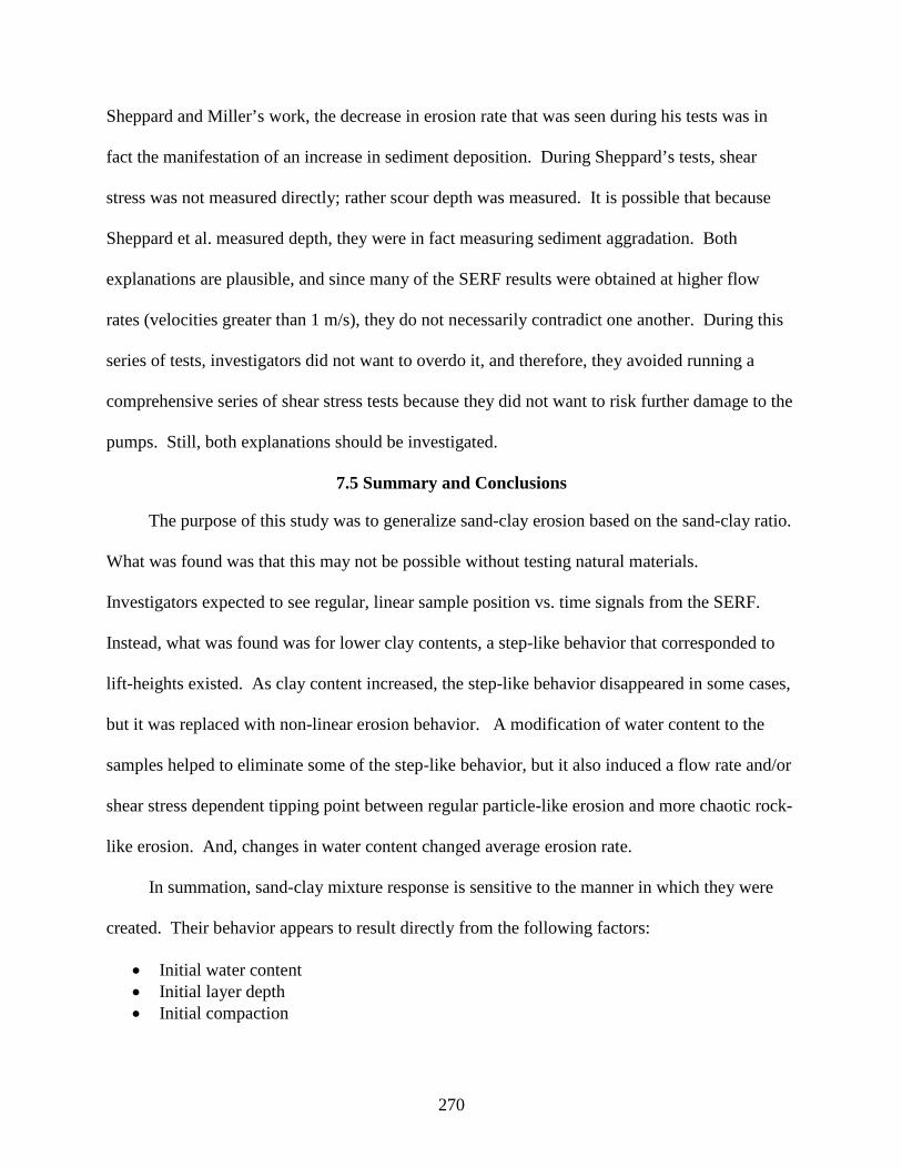
270

Sheppard and Miller’s work, the decrease in erosion rate that was seen during his tests was in

fact the manifestation of an increase in sediment deposition. During Sheppard’s tests, shear

stress was not measured directly; rather scour depth was measured. It is possible that because

Sheppard et al. measured depth, they were in fact measuring sediment aggradation. Both

explanations are plausible, and since many of the SERF results were obtained at higher flow

rates (velocities greater than 1 m/s), they do not necessarily contradict one another. During this

series of tests, investigators did not want to overdo it, and therefore, they avoided running a

comprehensive series of shear stress tests because they did not want to risk further damage to the

pumps. Still, both explanations should be investigated.


The purpose of this study was to generalize sand-clay erosion based on the sand-clay ratio.

What was found was that this may not be possible without testing natural materials.

Investigators expected to see regular, linear sample position vs. time signals from the SERF.

Instead, what was found was for lower clay contents, a step-like behavior that corresponded to

lift-heights existed. As clay content increased, the step-like behavior disappeared in some cases,

but it was replaced with non-linear erosion behavior. A modification of water content to the

samples helped to eliminate some of the step-like behavior, but it also induced a flow rate and/or

shear stress dependent tipping point between regular particle-like erosion and more chaotic rock-

like erosion. And, changes in water content changed average erosion rate.

In summation, sand-clay mixture response is sensitive to the manner in which they were

created. Their behavior appears to result directly from the following factors:

• Initial water content • Initial layer depth • Initial compaction

271

These variables appear to supersede variables that would be expected to govern the sand-

clay erosion problem: the sand-clay ratio. The conclusion of this study is that it should be

possible to engineer sand-clay materials to respond in a variety of different ways. The question

is which one of these response mechanisms most effectively corresponds to natural conditions?

Until this question is answered, further testing is not justified.

Other conclusions from this study are as follows:

1. Generally, it appears as though an increase in initial water content decreases erosion rate. It would be interesting to see if there is some threshold – i.e. does an increase in initial water content decrease erosion rate to a certain maximum and then does erosion rate increase again?

2. Likewise, is there a lower threshold limit? Below a certain initial water content, can a minimum erosion rate vs. shear stress relationship be found for sand-clay mixtures such that erosion rate is maximized for a given shear stress.

3. Solving (1) and (2) above may provide designers with an erosion rate range for a given shear stress based on sand-clay content. This could be useful for design purposes.

4. Although unintended, work during this study did provide information regarding the effects of suspended sediment on shear stresses. Shear stresses are not necessarily attenuated by the presence of suspended sediment. This may contradict earlier work by Sheppard et al. (2006b), and this discrepancy should be investigated.

5. Shear stresses appear to correspond to the theory that increasing roughness causes an increase in shear stress. This confirms work in Chapter 4 and also shows that without a shear stress sensor, the Moody Diagram is the most effective method for estimating shear stress in a flume-style erosion rate testing device.

7.6 Future and Ongoing Work

One phase of study that should be investigated further is the question of the suspended

sediment effects on bed shear stress. Results from this study contradict earlier work, and this

discrepancy needs to be addressed. This could be due to lab scaling effects, the fact that a flat

wall instead of a roughened surface was used during this study, or other unknown factors.

Currently, FDOT is running a series of triaxial tests on several sand-clay mixtures prepared

in the methods outlined in this Chapter. Work from this study will be presented in a student’s

272

future Honor’s Thesis. It will be interesting to see if preparation method affects the behavior of

sand-clay mixtures when using a more traditional test. Generally, triaxial test should be

repeatable for samples that are similar. If this is the case, it may be possible to use modified

triaxial data to engineer samples so that they respond like natural material from a triaxial test

perspective. If triaxial behavior can be matched, it may hold the key to matching erosion

behavior to natural materials.

The most important thing moving forward is to determine how actual sand-clay samples

behave. Samples during this study appear to correspond to Westergard theory where individual

layers are important. Do actual field samples behave similarly? The RETA cannot answer this

question, but future SERF tests can. If actual sand-clay mixtures show a dependence on

layering, using the RETA for development of sand-clay sediment transport functions is

inappropriate.

Another effect that was ignored during this study was the effect of consolidation. This

needs to be examined as well. Does consolidation play any role in either suppressing or

enhancing the layered-like behavior seen here? If it suppresses layered-like behavior, and it can

do so rather quickly, perhaps the layered behavior is a moot point. For example, if 24 hours of

consolidation reduces layering by a certain factor, this may show that there is no need to take

layering into account.

This ignores the initial water content dependence seen during this study, but perhaps that is

not that important either. Under natural conditions, sediment is saturated as it is deposited

(under a stream erosion scenario). Perhaps, it would be beneficial to prepare samples as

“naturally as possible.” This means, mix sand and clay in water, let it sit for a while (30 days or

more), and form a sample under its own self weight. Then, extract this sample, and test the

273

erosion rate on it. This may prove to be the most effective way to mimic field behavior in the

future.

274

Table 7-1. Density Profile Results Sample

Designation Water

Content Times

Optimum

Clay Content

(%)

Number of Lifts

Average Dry

Denisty (g/cm3)

Average Wet

Density (gm/cm3)

Dry Density Standard Deviation (g/cm3)

Wet Density Standard Deviation (g/cm3)

I 1x 25 1 1.70 1.91 0.070 0.077 II 1x 25 1 1.54 1.77 0.111 0.117 III 1x 25 2 1.53 1.76 0.125 0.133 IV 1x 25 2 1.53 1.84 0.213 0.234 V 1x 25 4 1.52 1.75 0.166 0.789 VI 1x 25 4 1.52 1.75 0.144 0.160 VII 2x 25 4 1.70 2.07 0.277 0.339 VIII 1x 25 8 1.58 1.81 0.074 0.089 IX 1x 50 4 1.44 1.83 0.162 0.175 X 1x 50 4 1.39 1.75 0.127 0.154 XI 1x 75 4 1.20 1.57 0.276 0.313

Figure 7-1. Grain Size Distribution for Sand Used During Sand-Clay Tests

0.00%

10.00%

20.00%

30.00%

40.00%

50.00%

60.00%

70.00%

80.00%

90.00%

100.00%

0.010.101.0010.00

Perc

ent P

assi

ng

Grain Size (mm)

275

Figure 7-2. Grain Size Distribution for EPK Used During Sand-Clay Tests

Figure 7-3. Optimum Water Content vs. Clay Content

0.00%

10.00%

20.00%

30.00%

40.00%

50.00%

60.00%

70.00%

80.00%

90.00%

100.00%

0.010.101.0010.00100.00

Perc

ent P

assi

ng

Grain Size (µm)

y = 0.0019x + 0.0652R² = 0.925

0.00%

5.00%

10.00%

15.00%

20.00%

25.00%

30.00%

0 20 40 60 80 100

Opt

imum

Wat

er C

onte

nt (%

)

Clay Content (%)

276

Figure 7-4. Shear Stress vs. Velocity for 0% Clay Epoxy Glued Disc

Figure 7-5. Shear Stress vs. Velocity for 12.5% Clay Epoxy Glued Disc

1 1.5 2 2.5 3 3.5 4 4.5 5 5.5 60

10

20

30

40

50

60

70

80

90

100

Velocity (m/s)

She

ar S

tress

(Pa)

y(x) = a x n̂a = 3.6357n = 1.8813R = 0.98686 (lin)

1 1.5 2 2.5 3 3.5 4 4.5 5 5.5 60

10

20

30

40

50

60

70

80

90

Velocity (m/s)

She

ar S

tress

(Pa)

y(x) = a x n̂a = 2.934n = 1.9836R = 0.99727 (lin)

277



1 1.5 2 2.5 3 3.5 4 4.5 5 5.5 60

10

20

30

40

50

60

70

80

90

Velocity (m/s)

She

ar S

tress

(Pa)

y(x) = a x n̂a = 2.7442n = 1.9906R = 0.9964 (lin)

1 1.5 2 2.5 3 3.5 4 4.5 5 5.5 60

10

20

30

40

50

60

70

80

90

Velocity (m/s)

She

ar S

tress

(Pa)

y(x) = a x n̂a = 2.9093n = 1.9438R = 0.99568 (lin)

278



1 2 3 4 5 6 70

10

20

30

40

50

60

70

80

90

Velocity (m/s)

She

ar S

tress

(Pa)

y(x) = a x n̂a = 5.1915n = 1.3883R = 0.88425 (lin)

-1 0 1 2 3 4 5 6 70

10

20

30

40

50

60

70

80

Velocity (m/s)

She

ar S

tress

(Pa)

y(x) = a x n̂a = 2.3712n = 1.8262R = 0.99586 (lin)

279



-1 0 1 2 3 4 5 6 70

10

20

30

40

50

60

Velocity (m/s)

She

ar S

tress

(Pa)

y(x) = a x n̂a = 1.9533n = 1.7323R = 0.9819 (lin)

-1 0 1 2 3 4 5 6 70

10

20

30

40

50

60

Velocity (m/s)

She

ar S

tress

(Pa)

y(x) = a x n̂a = 1.4779n = 1.6812R = 0.85282 (lin)

280


Figure 7-13. Summary Chart Showing Best-Fit Lines for Sand-Clay Epoxy Glued Discs

0 2 4 6 8 10 12 140

10

20

30

40

50

60

70

80

90

Velocity (m/s)

She

ar S

tress

(Pa)

y(x) = a x n̂a = 2.4385n = 1.3798R = 0.92919 (lin)

0 1 2 3 4 5 6 7 8 9 100

10

20

30

40

50

60

70

80

90

100

Velocity (m/s)

She

ar S

tress

(Pa)

0% Clay12.5% Clay25% Clay37.5% Clay50% Clay62.5% Clay75% Clay87.5% Clay100% Clay

281

Figure 7-14. Shear Stress vs. Velocity for 0% Clay Fiberglass Resin Test Disc

Figure 7-15. Shear Stress vs. Velocity for 12.5% Clay Fiberglass Resin Test Disc

-1 0 1 2 3 4 5 6 70

10

20

30

40

50

60

70

80

90

Velocity (m/s)

She

ar S

tress

(Pa)

y(x) = a x n̂a = 3.6319n = 1.723R = 0.98538 (lin)

-1 0 1 2 3 4 5 6 70

10

20

30

40

50

60

70

80

90

100

Velocity (m/s)

She

ar S

tress

(Pa)

y(x) = a x n̂a = 4.1463n = 1.7097R = 0.98693 (lin)

282



-1 0 1 2 3 4 5 6 70

10

20

30

40

50

60

70

80

90

Velocity (m/s)

She

ar S

tress

(Pa)

y(x) = a x n̂a = 2.5273n = 1.9055R = 0.99127 (lin)

-1 0 1 2 3 4 5 6 70

10

20

30

40

50

60

70

80

90

100

Velocity (m/s)

She

ar S

tress

(Pa)

y(x) = a x n̂a = 3.2161n = 1.848R = 0.98056 (lin)

283



-1 0 1 2 3 4 5 6 70

10

20

30

40

50

60

70

80

90

Velocity (m/s)

She

ar S

tress

(Pa)

y(x) = a x n̂a = 2.8309n = 1.7545R = 0.94202 (lin)

-1 0 1 2 3 4 5 6 70

10

20

30

40

50

60

70

80

90

Velocity (m/s)

She

ar S

tress

(Pa)

y(x) = a x n̂a = 2.8231n = 1.8371R = 0.99484 (lin)

284



-1 0 1 2 3 4 5 6 70

10

20

30

40

50

60

Velocity (m/s)

She

ar S

tress

(Pa)

y(x) = a x n̂a = 1.6917n = 1.8772R = 0.95905 (lin)

-1 0 1 2 3 4 5 6 70

10

20

30

40

50

60

70

80

90

100

Velocity (m/s)

She

ar S

tress

(Pa)

y(x) = a x n̂a = 2.8901n = 1.8322R = 0.97378 (lin)

285


Figure 7-23. Summary Chart Showing Best-Fit Lines for Sand-Clay Fiberglass Resin Discs

-1 0 1 2 3 4 5 6 70

10

20

30

40

50

60

Velocity (m/s)

She

ar S

tress

(Pa)

y(x) = a x n̂a = 2.8901n = 1.8322R = 0.97378 (lin)

y(x) = a x n̂a = 2.0237n = 1.6828R = 0.96004 (lin)

0 1 2 3 4 5 6 7 8 9 100

10

20

30

40

50

60

70

80

90

100

Velocity (m/s)

She

ar S

tress

(Pa)

0% Clay12.5% Clay25% Clay37.5% Clay50% Clay62.5% Clay75% Clay87.5% Clay100% Clay

286

Figure 7-24. Trammel’s 2004 Data Overlaid with Data from this Study

Figure 7-25. Erosion Rate vs. Shear Stress for 100% Sand Sample

0 0.5 1 1.5 2 2.5 3 3.5 40

0.1

0.2

0.3

0.4

0.5

0.6

Pump Frequency (Hz)

She

ar S

tress

(Pa)

Trammel 0.921 mm DataTrammel 0.508 mm DataCrowley 1.0 mm DataCrowley 0.50 mm Data

0 0.5 1 1.5 2 2.5 3 3.5 4 4.50

0.02

0.04

0.06

0.08

0.1

0.12

0.14

0.16

0.18

0.2

Shear Stress (Pa)

Ero

sion

Rat

e (m

/yr)

y(x) = a0 + a1 x + a2 x 2̂a0 = -0.0095099a1 = 0.0080322a2 = 0.0075811

R = 0.92172 (lin)

287

Figure 7-26. Non-Dimensionalized Erosion Rate vs. Shear Stress for 100% Sand Sample

Figure 7-27. Sample Position vs. Time for 25% Clay Mixture at 13.4 Pa

0 1 2 3 4 5 6 7 8 9 100

1

2

3

4

5

6

7

8

9

10

taub/tauc

E/(M

*tau

c)y(x) = a0 + a1 x + a2 x 2̂a0 = -0.50807a1 = 0.18345a2 = 0.073791

R = 0.92172 (lin)

0 50 100 150 200 250 300 350 4000

2

4

6

8

10

12

Time (s)

Sam

ple

Pos

ition

(cm

)

288



0 20 40 60 80 100 120 1400

1

2

3

4

5

6

7

8

9

Time (s)

Sam

ple

Pos

ition

(cm

)

0 100 200 300 400 500 6000

1

2

3

4

5

6

7

8

Time (s)

Sam

ple

Pos

ition

(cm

)

289

Figure 7-30. Sample Position vs. Time for 25% Clay Sample at 30.0 Pa


0 50 100 150 200 250 300 350 4000

2

4

6

8

10

12

Time (s)

Sam

ple

Pos

ition

(cm

)

0 20 40 60 80 100 120 140 160 180 2000

2

4

6

8

10

12

14

Time (s)

Sam

ple

Pos

ition

(cm

)

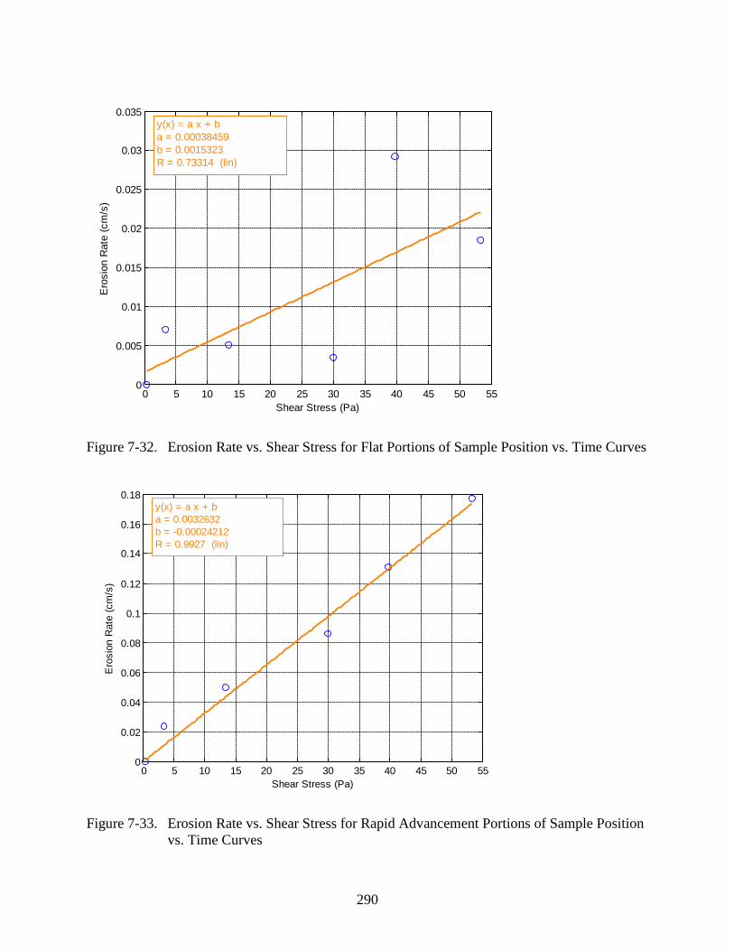
290

Figure 7-32. Erosion Rate vs. Shear Stress for Flat Portions of Sample Position vs. Time Curves

Figure 7-33. Erosion Rate vs. Shear Stress for Rapid Advancement Portions of Sample Position vs. Time Curves

0 5 10 15 20 25 30 35 40 45 50 550

0.005

0.01

0.015

0.02

0.025

0.03

0.035

Shear Stress (Pa)

Ero

sion

Rat

e (c

m/s

)

y(x) = a x + ba = 0.00038459b = 0.0015323R = 0.73314 (lin)

0 5 10 15 20 25 30 35 40 45 50 550

0.02

0.04

0.06

0.08

0.1

0.12

0.14

0.16

0.18

Shear Stress (Pa)

Ero

sion

Rat

e (c

m/s

)

y(x) = a x + ba = 0.0032632b = -0.00024212R = 0.9927 (lin)

291

Figure 7-34. Two-lift test at 13.4 Pa.

Figure 7-35. Sample Position vs. Time for 25% Clay Mixture Using Double Optimum Water Content

0 200 400 600 800 1000 1200 1400-12

-11

-10

-9

-8

-7

-6

-5

-4

-3x 10

4

Time (s)

Sam

ple

Pos

ition

(cm

)

0 1000 2000 3000 4000 5000 60000

2

4

6

8

10

12

Time (s)

Pos

ition

(cm

)

25.0 Pa11.5 Pa

y(x) = a x + ba = 0.023397b = -1.184R = 0.98784 (lin)

y(x) = a x + ba = 0.0010716b = 0.17626R = 0.9913 (lin)

292

Figure 7-36. Sample Position vs. Time for 50% Clay Mixtures


0 100 200 300 400 500 600 700 800 900 10000

2

4

6

8

10

12

Time (s)

Sam

ple

Pos

ition

(cm

)

2.94 Pa4.40 Pa5.99 Pa5.99 Pa15.69 Pa27.54 Pa41.07 Pa

0 10 20 30 40 50 60 70 80 90 1000

1

2

3

4

5

6

7

8

Time (s)

Sam

ple

Pos

ition

(cm

)

293

Figure 7-38. Zoom-in on First 90 Seconds of Sample Position vs. Time Curves

Figure 7-39. Sample Position vs. Time for 50% Clay Mixture at Double Optimum Water Content

10 20 30 40 50 60 70 80 900

0.2

0.4

0.6

0.8

1

1.2

1.4

1.6

1.8

Time (s)

Sam

ple

Pos

ition

(cm

)

2.94 Pa4.40 Pa5.99 Pa5.99 Pa15.69 Pa27.54 Pa41.07 Pa

0 200 400 600 800 1000 1200 1400 1600 1800 2000-2

0

2

4

6

8

10

12

Time (s)

Sam

ple

Pos

ition

(cm

)

27.54 Pa34.11 Pa41.07 Pa55.98 Pa

294

Figure 7-40. Sample Position vs. Time for 75% Clay Mixture Mixed at Optimum Water Content

Figure 7-41. Sample Position vs. Time for 75% Clay Mixture Mixed at Double the Optimum Water Content

0 200 400 600 800 1000 1200 1400 1600 18000

2

4

6

8

10

12

Time (s)

Sam

ple

Pos

ition

(cm

)

2.34 Pa4.72 Pa7.76 Pa15.67 Pa25.80 Pa

0 1000 2000 3000 4000 5000 60000

2

4

6

8

10

12

14

Time (s)

Sam

ple

Pos

ition

(cm

)

7.76 Pa11.42 Pa15.67 Pa

295

Figure 7-42. Sample Position vs. Time for 100% Clay Mixed at Optimum Water Content

Figure 7-43. Sample Position vs. Time for 100% Clay Mixed at Double Optimum Water Content

0 200 400 600 800 1000 1200 1400 1600 1800 20000

2

4

6

8

10

12100% Clay

Time (s)

Pis

ton

Pos

itiio

n (c

m)

19.41 Pa22.84 Pa26.41 Pa

0 100 200 300 400 500 600 700 8000

2

4

6

8

10

12

Time (s)

Sam

ple

Pos

ition

(cm

)

17.76 Pa19.41 Pa26.41 Pa

296

Figure 7-44. Density Profile for Sample I

Figure 7-45. Density Profile for Sample II

1 1.5 2 2.5 30

2

4

6

8

10

12

14

Density(g/cm3

Hei

ght (

cm)

Wet DensityDry Density

1 1.5 2 2.5 30

2

4

6

8

10

12

14

Density(g/cm3

Hei

ght (

cm)


297

Figure 7-46. Density Profile for Sample III

Figure 7-47. Density Profile for Sample IV

1 1.5 2 2.5 30

2

4

6

8

10

12

14

Density(g/cm3

Hei

ght (

cm)


1 1.5 2 2.5 30

2

4

6

8

10

12

14

Density(g/cm3

Hei

ght (

cm)


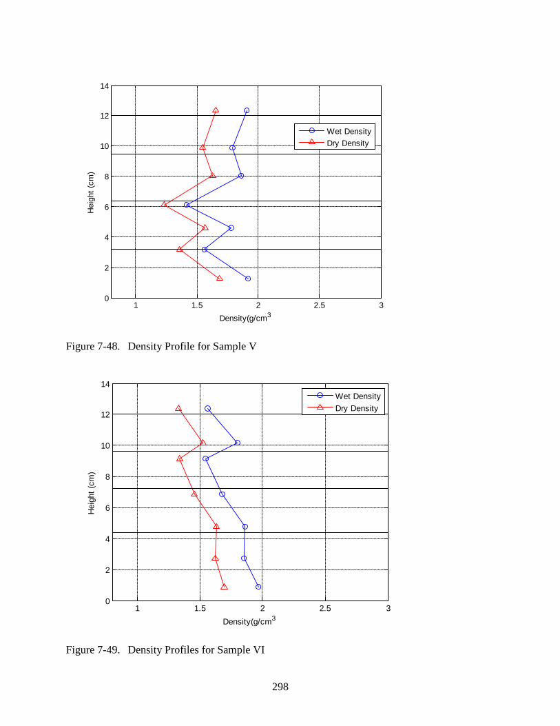
298

Figure 7-48. Density Profile for Sample V

Figure 7-49. Density Profiles for Sample VI

1 1.5 2 2.5 30

2

4

6

8

10

12

14

Density(g/cm3

Hei

ght (

cm)


1 1.5 2 2.5 30

2

4

6

8

10

12

14

Density(g/cm3

Hei

ght (

cm)


299

Figure 7-50. Density Profiles for Sample VII

Figure 7-51. Density Profiles for Sample VIII

1 1.5 2 2.5 30

2

4

6

8

10

12

14

Density(g/cm3

Hei

ght (

cm)


1 1.5 2 2.5 30

2

4

6

8

10

12

14

Density(g/cm3

Hei

ght (

cm)


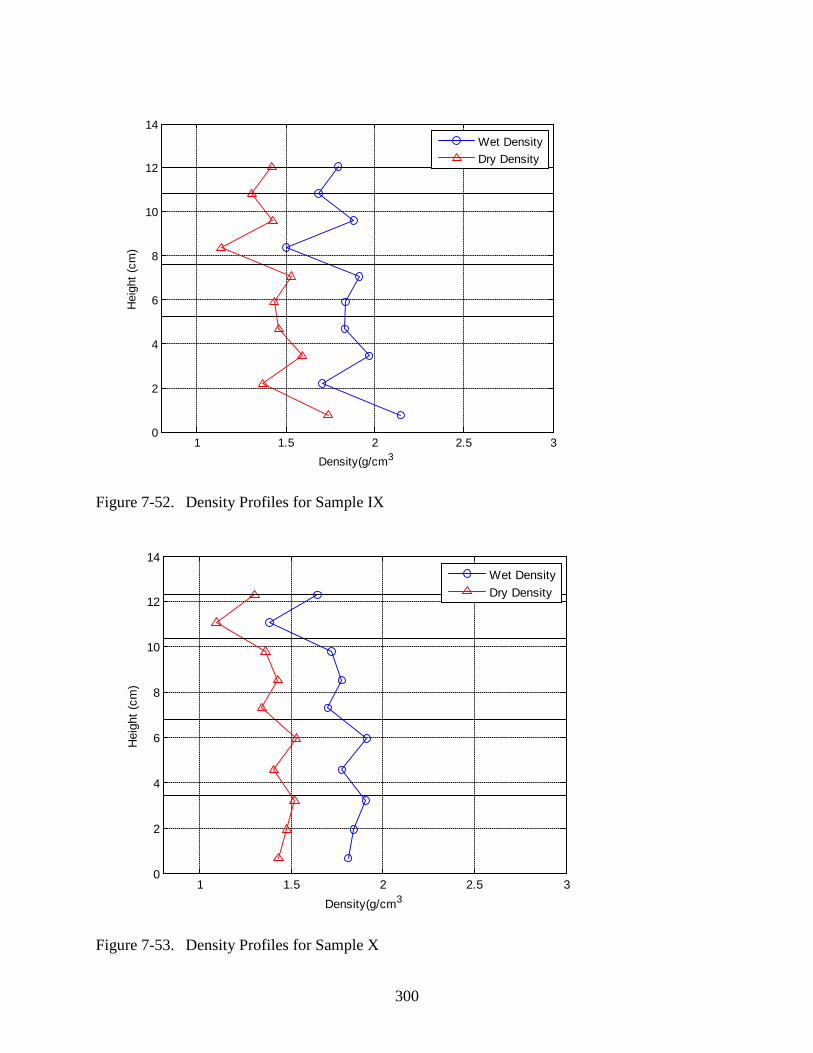
300

Figure 7-52. Density Profiles for Sample IX

Figure 7-53. Density Profiles for Sample X

1 1.5 2 2.5 30

2

4

6

8

10

12

14

Density(g/cm3

Hei

ght (

cm)


1 1.5 2 2.5 30

2

4

6

8

10

12

14

Density(g/cm3

Hei

ght (

cm)


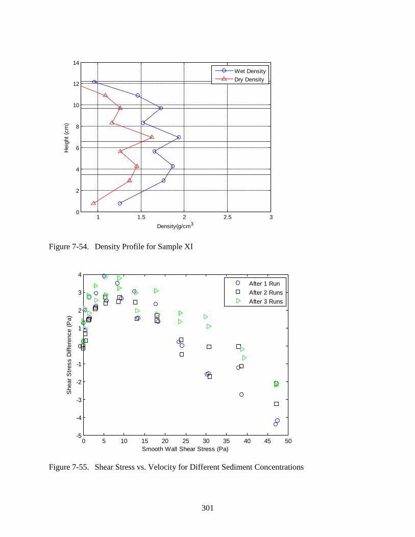
301

Figure 7-54. Density Profile for Sample XI

Figure 7-55. Shear Stress vs. Velocity for Different Sediment Concentrations

1 1.5 2 2.5 30

2

4

6

8

10

12

14

Density(g/cm3

Hei

ght (

cm)


0 5 10 15 20 25 30 35 40 45 50-5

-4

-3

-2

-1

0

1

2

3

4

Smooth Wall Shear Stress (Pa)

She

ar S

tress

Diff

eren

ce (P

a)

After 1 RunAfter 2 RunsAfter 3 Runs

302

CHAPTER 8 SUMMARY AND FUTURE WORK

8.1 Summary

8.1.1 Review of Goals for This Study

The purpose of this research was to aid in the development of erosion rate functions for use

in a similar-style-Miller-Sheppard approach or EFA-SRICOS approach for predicting local scour

depths. The specific goals for this were to:

1. Develop equipment to improve accuracy of erosion and shear stress measurements for a wide range of eroding bed materials.

2. Use these equipment upgrades and other analytical techniques to comment quantitatively on older methods for measuring these parameters by running a series of tests with the new equipment.

3. Use these new measurements and older results to determine if erosion rate can be related to any other existing common geotechnical parameters.

4. Use the new equipment to develop a series of erosion rate-shear stress curves for sand clay mixtures. Under natural conditions, it is rare to find a bed material that is purely cohesive or purely non-cohesive. Instead, usually sand is interspersed with clay particles or vice versa. Previous research has looked only to classify erosion rate-shear stress curves under conditions where a uniform material is present, but because this is rarely the case, erosion properties of mixtures are investigated.

8.1.2 Summary of Work

To achieve these goals, the following was accomplished during this project:

1. The Sediment Erosion Rate Flume (SERF) was enhanced and improved. Significant upgrades to the device include

a. A laser system

b. A new shear stress measurement system

c. A vortex generation system

d. Computer upgrades

e. Software upgrades

303

f. Additionally, a sand injection/control system was designed. Although funding for this system does not yet exist, when funding becomes available, installation of this system should be relatively straight-forward.

2. A series of tests were conducted with the new shear stress sensor in the SERF to determine the apparent most effective method for estimating shear stress in a flume-style erosion rate testing device.

3. A synthetic material, Bull Gator Rock, was designed so that it could be tested in both the SERF and the Rotating Erosion Testing Apparatus (RETA).

4. Bull Gator Rock testing revealed the presence of rock-like erosion, which is difficult to analyze with present equipment that is only designed to measure erosion rate and shear stress. Therefore, the entire RETA database was filtered and used in conjunction with analytical equations to verify whether or not the device was working properly.

5. A series of tests was run on a variety of sand-clay mixtures in an attempt to generalize sand-clay mixture erosion behavior as a function of sand-clay ratio.

8.2 Conclusions

The following is a list of conclusions from this project:

1. The laser-leveling system is an effective means of maintaining a sample level during an erosion rate test in a flume-style device, especially during clay and sand-clay tests.

2. The temperature control system in the SERF was effective at holding temperature within +/-2oC.

3. The sediment control system was unable to keep up with rapid erosion rates.

4. Tests with the new shear sensor showed that as sample roughness increases for a given flow rate, corresponding shear stress also appears to increase.

5. In the absence of a shear stress sensor, the most effective alternative means for estimating shear stress on an eroding sample in a flume-style testing device is to use a Moody Diagram or Colebrook Equation. The roughness factor in the Colebrook Equation should be equal to one-half the median sediment diameter. Flat-wall assumptions for predicting shear stress under-predict shear stress, especially at higher roughness and flow velocities.

6. Bull Gator Rock may be a promising material for use in comparing results between different erosion rate testing devices if somehow water content can be increased. Currently, it appears that the bottom-up approach will produce a nearly-uniform material if limestone aggregate is similarly nearly uniform. However, Gator Rock tests also showed that obtaining a water content greater than ~20% using a bottom-up technique may not be possible.

304

7. The RETA database showed that under special conditions where erosion conditions correspond to a direct erosion rate vs. shear stress relationship, results from the RETA correspond to results from equations that fit the Ariathurai equation form accurately.

8. RETA database analysis showed that there is an approximately even split between materials that behave with a direct erosion rate vs. shear stress relationship and materials that do not. For materials that do not obey a direct relationship, rock-like erosion described by The Stream Power Model is likely the culprit. When rock-like erosion is present, current equipment limitations do not allow for prediction or analysis of this erosion mode. This is significant because generally, rock-like erosion appears to occur an order of magnitude slower than particle-like erosion.

9. RETA database analysis showed that for the special case of particle-like erosion, correlations may exist between erosion rate constant, critical shear stress, and material cohesive strength.

10. Tests on sand-clay mixtures showed that sand-clay mixture erosion behavior is dependent on initial water content when the sample was formed, compactive effort as the sample was formed, and layering thickness as the sample was formed.

11. Sand-clay mixtures exhibit a combination of rock-like and particle-like erosion qualities even though sand-clay mixtures would usually not be described as rock-like materials.

12. Sand-clay mixtures tended to exhibit the opposite effect as stiffer RETA materials in terms of erosion rates for stronger materials. With sand-clay mixtures, when initial water content increased, samples were created that were qualitatively weaker in compression and tension. These samples exhibited more resistance to erosion than samples that were stiffer and stronger in compression and tension.

13. Recirculating sand in suspension in the SERF does not appear to affect shear stresses on a smooth plate compared to what shear stresses would have been under clear water conditions.

8.3 Future Work

The following is a proposed progression of future work. Proposed work discussed here

will help to further improve the SERF, aid in developing erosion rate and shear stress

relationships, and help to predict when (or if) particle-like or rock-like erosion will occur.

8.3.1 Essential Final Improvements to the SERF

Before the rock-like vs. particle-like erosion question can be answered, essential final

improvements need to be made to the SERF. As discussed, when an erosion rate test is run, the

305

eroded material recirculates back through the flume; this issue is common with recirculating

flumes with a relatively small (1,100 gal.) reservoir tank.

This recirculating particle issue is troublesome for three reasons. First, due to the number

of variables associated with the erosion rate problem, researchers need to isolate them from one

another. The second and more important reason to add a high-capacity filter is that without it,

the SERF will probably be damaged. The pumps will be damaged because these sand-clay flocs

are essentially sand-blasting the centrifugal pumps’ impellers. Sometimes when the reservoir

tank is drained, rust particles are often seen interspersed with the sand-clay flocs. Since the

flume is made of aluminum, the rust particles must be from the cast iron pumps. This proves that

damage is already occurring. Towards the end of this project, one of the pumps’ mechanical

seals began leaking – which appears to indicate that damage due to recirculating sediment has

occurred.

The third reason to add a high-capacity filter is so that the sand injector can be installed,

tested, and used during tests. Installation of the sand injector will allow investigators to follow

up on tests shown in Section 7.4.4 so that definitive results can be obtained for the effects of

suspended sediment on shear stress.

If the filter is installed in the SERF, it makes sense to extend the device. Given the present

setup, the sand injector cannot be installed anywhere else other than where the paddlewheel

flowmeter is currently located. Presumably, a filter would have the same problem – the PVC

run-up to the rectangular portion of the flume is not long enough to accommodate more than one

device. Therefore, PVC pipes leading into the rectangular portion of the device should be

extended in conjunction with the filter installation so that as water passes through the flume it

306

passes through the pumps, through the filter, past the flowmeter, through the sand injector, and

finally into the rectangular portion of the flume.

8.3.2 Non-Essential Final Improvements to the SERF

Although the following improvements to the SERF are listed as “non-essential” their

inclusion is beneficial because these improvements will improve the accuracy of the device.

From 2003-2006, three of the twelve crystals in the SEATEK array broke; it is unclear why this

happened, but what is clear is that the array should be replaced or fixed so that the crystals work

properly. It may be advantageous to replace the array completely so that a faster mechanism can

be installed. Computer technology has advanced in the past ten years, and the current ultrasonic

array is only capable of sending an output signal once every second. A faster digital signal will

allow for less time in between steps, which in turn will allow for a more level sample at the

bottom of the SERF.

Secondly, the three-laser leveling system should be replaced with a light-sheet design.

When certain materials erode under rock-like conditions, often differential erosion rates are

present such that the back-face of the sample erodes faster than the front or vice-versa. When the

lasers are used as a stand-alone mechanism for measuring sample flushness (as is necessary with

clays), a simple array of three lasers is not enough to account for this. A better design would be

to illuminate one side of the sample with a light sheet and install corresponding photoelectric

sensors on the other side. Then, when a certain percentage of the light is seen (such as 50%), the

sample would advance. This would provide a much more accurate method of leveling sand-clay

mixtures with the flume’s bottom.

The third improvement is quite simple – a new computer should be added to the SERF

control room. The present computer system is old, and sometimes it cannot keep up with a

307

rapidly eroding sample. A new computer running on a 64 bit operating system with more

memory is needed.

The fourth improvement that should be made to the SERF is that the stepper motor

assembly needs to be redesigned. The current design uses a stepper-motor assembly where the

maximum force against the piston is approximately 400 lb. Over time, due to normal wear and

tear, the amount of force that can be applied to the piston decreases. Eventually, the motor

cannot provide enough force to overcome the friction between the piston’s O-rings and the side

walls of the piston-casing. What makes matters worse is that during an erosion test, small pieces

of sediment get stuck in the tiny gap between the piston and its housing. Although these pieces

of sediment are tiny, they are large enough to increase the friction factor between the piston and

its housing to the point where the piston can no longer move. When this happens, the motor’s

gears begin to grind against one another, and eventually the motor burns out. During longer-

duration testing (as seen with rock-like material and Gator Rock), this is especially an issue,

because as this is happening the motor heats up rapidly. To prevent this, the motor needs to be

replaced by a heavy duty linear actuator. These devices are designed for repeated loading, and

will be better able to apply a higher force to the piston. Since 2006, three motors have burned

out during SERF testing due to normal motor usage combined with harsh experimental

conditions. Rather than spend money on new motors every 18 months, an improvement should

be implemented.

The fifth improvement that should be made to the SERF is to install an ultra-sonic Doppler

radar (UDV) system for measuring velocity profiles in the device. This system will allow

researchers to verify that flow conditions in the SERF are fully developed.

308

8.3.3 Determine Erosion Patterns for Natural Sand-Clay Mixtures

Once final improvements and enhancements have been made, the next step is to determine

how natural sand-clay mixtures behave when subjected to SERF testing. As discussed,

sensitivity exists between erosion rates and sample preparation methods. Rather than engineer a

series of materials to behave differently, it makes more sense to mimic natural erosion patterns

during future tests. Therefore, natural materials need to be obtained and tested in the flume to

see how they react to erosion rate testing. These materials should be subjected to a series of tests

under clear water and simulated live-bed conditions. Because the filter will have been installed,

these tests will now be possible. These samples also should be subjected to tensile and

compressive strength testing ( if strong enough) to determine if the relationships developed for

erosion rate as a function of cohesion presented in Chapter 6 is still valid.

8.3.4 Roughness Number Tests or Improved Testing Apparatus

As discussed in Chapter 3, shear stress is sensitive to sample roughness. Because it is not

yet possible to measure shear stress at the same time as erosion rate, the question as to how to

properly measure erosion rates and shear stresses of natural samples is difficult to answer. If it

continues to be impossible to measure erosion rate and shear stress at the same time, then the

most effective alternative is to measure a sample’s roughness and use that to approximate the

shear stress on it.

Curves have already been developed for shear stress as a function of flow rate and

sediment diameter. Using high-resolution photography (UF has a device that can do this), it

should be possible to measure the roughness associated with these samples. Then, given a

natural sample, the cameras can be used to approximate its roughness and existing shear stress

curves can be used to determine shear stresses associated with given flow rates.

309

Alternatively, using the principles from the shear stress sensor, it may be possible to

engineer a device that can measure erosion rate and shear stress at the same time. Both

approaches should be investigated.

8.3.5 Normal Stress Measurements in SERF

Preceding discussion assumes particle-like erosion, but as discussed several times, for

cohesive material, a strict particle-like erosion mode is hardly ever seen. The next research step

hinges on how natural sand-clay bed materials behave. Hence, first one needs to measure the

normal stresses on different sand-clay mixtures to determine under what conditions rock-like

erosion dominates. Presumably, if rock-like erosion were to dominate, the normal stresses on a

sample should be larger than they would be under particle-like conditions.

If this is not the case, then it may be possible to find a sediment property that would

indicate whether or not rock-like erosion is likely. For example, it should be possible to prepare

a series of sediments at the same sand-clay ratio, same lift-heights, and different water contents.

Based on results presented in Chapter 7, eventually at a certain initial water content, rock-like

erosion should become important. Likewise beyond this water content, rock-like erosion may

become less important. Similarly, there may be a threshold clay content where rock-like erosion

also begins to take an effect. Right now, it is obvious that rock-like rock erosion does not and

cannot occur for a 100% sand bed. At what clay content does it begin to become an issue?

Finding these threshold values specifically (this dissertation simply defined this as an important

variable and helped to bound the problem) may hold the key to explaining when rock-like

erosion will occur for a sand-clay mixture.

8.3.6 Normal Stress Measurements under Field Conditions

Because normal stress is caused by the fluctuating velocity component, and the turbulent

eddy mixing length is much shorter in the SERF than it is in nature, normal stress measurements

310

must be compared with normal stress measurements under field conditions to test their validity.

A field device or devices should be designed to measure both normal and shear stresses in an

actual streambed to answer these questions. Additionally, an upstream Acoustic Doppler Current

Profiler (ADCP) probe should be installed in this stream so that conditions can be monitored

continuously.

8.3.7 Computer Model

If researchers find that normal stresses are significant, then these field results should be

used to calibrate a computer model similar to Briaud’s model. The difference between this

model and Briaud’s is that instead of just returning a maximum shear stress value, this new

model may be able to return a normal stress value as well.

8.3.8 Summary of Proposed Future Progression

The preceding discussion is not a comprehensive discussion regarding the cohesive erosion

rate problem. Predicting erosion rate for cohesive sediments is complicated and the discussion

serves as a logical series of steps based on research presented in this dissertation.

311

APPENDIX A SCOUR DEPTHS IN NON-COHESIVE SOILS

A.1 Introduction

As discussed in Chapter 2, erosion of non-cohesive materials is a mode of particle erosion.

Erosion processes such as these may be analyzed using a simple force balance relationship.

When a non-cohesive particle is resting on the bed and water passes over top of it, the particle is

subjected to a drag force, FD and a lift force FL where the magnitude of these forces is a function

of the particle’s geometry. An expression for drag forces and lift forces has been developed such

that:

25.0 uACF yzDD ρ= (A-1)

25.0 uACF xyLL ρ= (A-2)

where Axy is the planform area of the particle, Ayz is the cross-sectional area of the particle, ρ is

the density of water, u is the fluid velocity, and CL and CD are experimentally determined drag

and lift coefficients.

Under non-erosion conditions, these drag forces and lift forces, plus the buoyant weights of

the particle are balanced by bed friction and the force of gravity. Under erosion conditions, the

flow velocity, u, must become high enough to cause the lift force, FL to overcome the force of

gravity; or u must become high enough for the drag force on the particle, FD to overcome the

force of static friction between the particle and the bed. When the lift force becomes larger than

the drag force, the particle is said to go into suspension whereas when the drag force overcomes

the friction force, the particle is said to be moving as part of the bed-load.

In 1936, Shields studied the minimum velocity required to initiate incipient motion of bed

particles of various sizes, and he developed a diagram similar to Figure A-1 where below the

312

purple line, there is no sediment motion and above the line, sediment will erode. The green line

(Developed by Bagnold in 1966) divides the bed load from the suspended load.

Although this analytical approach to solving the erosion problem is elegant, the

hydrodynamics in the vicinity of a scouring structure are complicated, and to date, a

comprehensive theoretical solution to the scour problem could not be found. To solve

analytically, flow conditions in the vicinity of a complex pier would need to be solved so that

one could determine when flow velocity exceeded the critical velocity of the bed material.

Because of the difficulties associated with solving for these hydrodynamic conditions, an

empirical approach has been used when solving for particle scour. The following is an analysis

of the existing empirical standards for estimating scour depths due to non-cohesive sediment

transport.

A.2 HEC-18: Basic Principles (Richardson and Davis 2001)

HEC-18 instructs an engineer to compute the scour effects from aggradation/degradation,

general scour, contraction scour, and local scour. Then, the effects from each of these

parameters are added and the total scour depth is computed.

A.2.1 HEC-18: Long Term Aggradation and Degradation (Richardson and Davis 2001)

Long term aggradation and degradation are computed by using a three-level fluvial system

approach. First, a qualitative determination regarding long-term stream stability is established

using general geomorphic and river mechanics relationships. Then, engineering analyses follow

where the probable behavior of the stream system is estimated. Finally, physical models or

computer models are to be used to predict quantitative changes to the streambed elevation.

According to HEC-18, acceptable computer models include Bridge Stream Tube Model for

Alluvial River Simulation (BRI-STARS) and USACE HEC-6, Scour and Deposition in Rivers

and Reservoirs computer model (Richardson and Davis 2001).

313

A.2.2 HEC-18: Contraction Scour (Richardson and Davis 2001)

To find the design contraction scour depth, first an engineer must determine if flow

upstream from a bridge or an obstruction is already transporting bed material. Therefore the

critical velocity for incipient motion, Vc, needs to be computed based on the upstream bed

material’s mean diameter, D50. According to HEC-18, critical velocity is computed using the

following equation:

3/16/1 DyKV uc = (A-3)

where Ku is a constant that is dependent on English or SI units (6.19 for SI units, 11.17 English

units), y is the average flow depth upstream from the bridge or obstruction, and D is the average

particle size. Once critical velocity is known, the engineer can compute determine whether clear

water (V < Vc and there are no particles in suspension) or live-bed (V > Vc and there are particles

in suspension) conditions are present.

For clear water conditions, contraction scour is computed using Equation A-4:

7/1

23/2

2

2

=

WDQK

ym

u (A-4)

where y2 is the equilibrium scour depth after contraction scour, Q is the discharge through the

obstruction, Dm is the diameter of the smallest nontransportable particle in the bed material

(1.25D50) in the contracted section, W is the bottom width of the contracted section minus the

pier widths, and Ku again is a constant that is unit dependent (0.025 for SI units and 0.0077 for

English units).

For live-bed conditions, contraction scour is computed using Equation A-5:

1

2

17/6

1

2

1

2k

WW

QQ

yy

= (A-5)

314

where y1 is the average depth in the upstream channel, y2 is the average depth in the contracted

section, Q1 is the flow in upstream channel, Q2 is the flow in the contracted channel, W1 is the

width of the upstream channel, W2 is the width of the contracted section, and k1 is an exponent

based on shear velocity in the upstream section and fall velocity of the bed material. k1 can be

determined via table A-1 and Equation A-6:

( ) 2/11

2/10* SgyV =

=

ρτ

(A-6)

where V* is the shear velocity, g is the acceleration due to gravity, τ0 is the shear stress on the

bed, ρ is the density of water, ω is the fall velocity as determined from Figure A-2, and S1 is the

slope of the energy grade line of the main channel.

A.2.3 HEC-18: Local Scour (Richardson 2001)

Local scour is computed with the underlying assumption that each parameter that affects

the final depth of the scour hole is independent of the other parameters. In other words, the

effects of angle of attack, shape of the pier, spacing between pier piles, bed conditions, and

armoring are computed separately. Then, these parameters are fit together with the following

equation:

43.01

35.01

4321 Fray

KKKKays

= (A-7)

where K1, is the correction factor due to pier shape, K2 is the correction factor for angle of attack,

K3 is the correction factor for the bed conditions (live bed or clear water), and K4 is the correction

factor for armoring; ys is the depth of the scour hole, a is the pier width and Fr1 is the Froude

Number defined by

2/1

1

11

=

gyV

Fr (A-8)

315

where V1 is the velocity upstream from the pier and y1 is the depth upstream from the pier

(Richardson and Davis 2001). The correction factor, K1 is calculated using Figure A-3 and Table

A-2. The correction factor K2 is computed using Equation A-9:

65.0

2 sincos

+=

θθ

aLK (A-9)

where θ is the attack angle, and L and a were previously defined as the length and width of the

pier respectively. The correction factor K3 is found using Table A-3. The correction factor K4 is

computed using a series of equations:

( ) 15.04 4.0 RVK = (A-10)

09550

501 >−

−=

icDcD

icDR VV

VVV (A-11)

xx cD

xicD V

aD

V053.0

645.0

= (A-12)

3/16/11 xucD DyKV

x= (A-13)

In these equations, VicDx is the approach velocity required to initiate scour at the pier for a given

grain size, Dx, and VcDx is the critical velocity for incipient motion for the grain size, Dx; y1 is the

depth of flow just upstream of the pier; V1 is the velocity of approach flow upstream of the pier,

and Ku us a constant that is unit-dependent (6.19 for SI and 11.17 for English). HEC-18

recommends a minimum value of K4 of 0.4.

The preceding equations assume a narrow pier. For wide piers, or piers that have multiple

piles or pile caps, the equations become somewhat more complicated. To compute scour for a

wide pier, an additional correction factor, Kw is introduced and Equation A-7is modified:

43.01

35.01

4321 Fray

KKKKKay

ws

= (A-14)

316

1for 58.2 65.034.0

<

=

cw V

VFrayK (A-15)

1for 0.1 25.013.0

≥

=

cw V

VFrayK (A-16)

When computing scour when there are multiple piles, a pile cap, and/or a pier involved,

scour is computed by adding the effects of scour due to these three components:

spgspcspiers yyyy ++= (A-17)

where yspier is the scour component from the pier stem, yspc is the scour component due to the pile

cap and yspg is the scour component due to the pile group. The equation for computing yspier is

similar to Equation A-18:

=

43.0

1

1

65.0

14321

1

0.2gyV

ya

KKKKKy

y pierhpier

spier (A-18)

The difference between Equation A-18 and Equation A-14 is the introduction Khpier, which is the

coefficient used to account for both the height of the pier stem above the bed and the shielding

effect by the pile cap overhanging distance f in front of the pier stem. Khpier is found by using

Figure A-4.

Scour from the pile cap is divided into two scenarios. On one hand, the bottom of the pile

cap may be above the bed and in the flow path. On the other hand the pile cap may be located on

or below the bed. When the pile cap is above the bed, the technique for computing scour is to

reduce the pile cap width to an equivalent pier depth and width, a*pc, using Figure A-5.

Then, scour for the pile cap component is computed using Equation A-19:

43.0

2

2

65.0

2

*

43212

0.2

=

gyV

ya

KKKKKy

y pcw

spc (A-19)

317

Under the scenario where the pile cap is on or below the bed, a slightly different series of

equations, Equation A-20, Equation A-21, and Equation A-22 are used instead:

43.065.0

24321

2

0.2

=

f

fpcw

spc

gy

Vya

KKKKKy

y (A-20)

+

+

=

193.10ln

193.10ln

22

s

s

f

f

Ky

Ky

VV

(A-21)

21xpier

f

yhy += (A-22)

In these equations, Vf is the average velocity in the flow zone below the top of the footing and yf

is the distance from the bed to the top of the footing. Figure A-6 is an illustration of these

parameters. When the footing is on or above the bed, there is no need to compute the scour

effect from the pile group. Therefore, under this scenario, Equation A-22 can be modified:

spcspiers yyy += (A-23)

The strategy for finding the scour component that results from a pile group is to represent

the pile group by an equivalent solid pier width, a*pg, which is found using Equation A-24:

mspprojpg KKaa =* (A-24)

Km is the number of rows factor, and it is equivalent to 1.0 for the general case of skewed or

staggered rows of piles. When piles are aligned, Km must be determined from Figure A-7. To

illustrate how to compute the projected pile group equivalent pier width, Figure A-8 is useful.

The coefficient of spacing, Ksp is found using Figure A-9. The scour component from the pile

group is computed using Equation A-25, Equation A-26, and Equation A-27. The pile group

high factor, Khpg is given in Figure A-10.

318

2213spcspier yy

yy ++= (A-25)

=

3

113 y

yVV (A-26)

2203spcspier yy

hh ++=

=

43.0

3

3

65.0

3

*

4313

0.2gyV

ya

KKKKy

y pghpg

spg (A-27)

A.2.4 HEC-18: Brief Discussion

The local scour equations from HEC-18 are based on a series of tests at CSU, and they are

empirical. Because these equations are empirical, after they were introduced, there was some

concern that they may need to be slightly adjusted. This will be discussed in the subsequent

section.

A.3 The Florida DOT Bridge Scour Manual

The FDOT Bridge Scour Manual (FDOTBSM) was published in 2005, and it is another

source that can be used to compute design scour depth. This document is similar to HEC-18 in

many respects; in both documents the scour component associated with long-term

aggradation/degradation, contraction scour, general scour, and local scour are computed

independently and added together. To compute total scour, the FDOTBSM uses the same

equations and recommendations as HEC-18 for scour components except for local scour.

A.3.1 Local Scour: Motivation for a Different Computation Algorithm

Computation of local scour is different in the FDOTBSM than it is in HEC-18. The

FDOTBSM argues that because the CSU equations (HEC-18 equations) are empirical and based

319

on small-scale laboratory data, they may yield different results when they are applied to

prototype scale structures. The hydrodynamics surrounding the scour problem would appear to

indicate that this is a valid concern, and an order of magnitude analysis can be used to illustrate

this point:

1.) Under field conditions: assume a typical bridge pier width of 1.0m and a typical grain

size of 1x10-4m; the ratio of grain size to pier width is on the order of 1x10-4m.

2.) Under laboratory conditions: grain size of sand cannot change because if the sand were

smaller, it would no longer be a sand. Instead, it would be a cohesive material like a

silt, and it would be affected by associated cohesive forces. However laboratory pier

width may be on the order of 1 cm. Therefore the ratio of grain size to pier width is

two orders of magnitude smaller – 1x10-2.

In 1988, Melville proposed a design method that allowed the designer to follow flow charts

to calculate the limiting armor velocity and the local scour depth. According to this study, the

maximum scour depth that can occur equals 2.4 times the pier diameter. However, when the

designer is dealing with shallow water, larger sediment grain sizes, and clear water conditions,

Melville proposed that this 2.4 factor should be reduced based on dimensionless flow velocity,

V/Vc; the ratio of flow depth to pier diameter, y0/D50; the ratio of pier diameter to sediment grain

size, b/D50; and shape and alignment factors (Melville and Sutherland1988).

In the early 2000’s, Dr. Sheppard of UF conducted three series of prototype-scale tests

under both clear-water and live-bed conditions (Sheppard, et al. 2004). The first series of tests,

which were conducted in Turners Falls, MA, tested scour depths of three pier sizes and three

sediment sizes over a range of depths and velocities under clear water conditions. An interesting

phenomenon was noticed during this study. The water supply for this flume study was taken

320

from a hydroelectric power plant reservoir, and there was no control over the amount of

suspended sediment in it. During testing, Sheppard noticed sudden increases in shear stresses

that were attributed to reduced levels of turbulence from increased suspended sediment load

during high runoff events such as snow melt. Sheppard reasoned that these suspended sediments

slowed or stalled the formation of equilibrium scour depths because the sediment helped to

dampen the turbulence. The implication here is that under live-bed conditions the equilibrium

scour depth may be lower than it would be under clear water conditions (Sheppard et al. 2004).

In 2004, Sheppard launched a second study concerning an additional pressure gradient

factor affecting the formation of local scour (Sheppard 2004). According to Sheppard, the

pressure field adjacent to the bed is determined by the pressure field in the main flow. When a

pier or another structure interrupts the flow, pressure gradients near the structure will impose

forces on sediment particles of a greater magnitude than drag forces because of the water flowing

around the sediment particles. Sheppard mathematically explored these pressure gradient forces

and their dependence on the D/D50; and he found that the magnitude of these forces caused by

this pressure gradients decreased as this ratio increased (Sheppard 2004). This observation

agreed with his previous experimental work (Slagle 2006).

Sheppard’s third study was conducted at the University of Auckland and its purpose was to

investigate live-bed local pier scour for a circular pile and compare calculated equilibrium scour

depths with those that are physically measured. Sheppard observed a decreased dependence of

normalized equilibrium scour on D/D50 at higher values of V/Vc where D is the pier width, D50 is

the median sediment grain size, V is the upstream flow velocity, and Vc is the sediment critical

velocity (Sheppard 2006b).

321

The combination of these tests helped in development of the equations in the FDOTBSM

for local scour. According to Slagle, these equations are the most successful at predicting the

local scour depth. Slagle says that the average percent difference in results between computed

scour depth and measured scour depth was 16.6%; the standard deviation was 18.2% (Slagle

2006).

A.3.2 FDOTBSM: Local Scour Equations (Florida DOT Bridge Scour Manual 2005)

For computing the design scour depth of a pier under clear-water conditions, pier, Equation

A-28 is used:

( ) ( )

+

−

=− 13.0

50*5.0

50*

50

24.0

*0

* /6.10/4.0

/ln75.11tanh5.2

DDDD

DDVV

Dy

Dy

c

x (A-28)

Equation A-28 is only appropriate when (0.47 < V/Vc < 1). Under live-bed conditions

(1<V/Vc<Vlp/Vc), equation A.3-2 is used to compute the design scour depth up until the live-bed

peak:

( ) ( )

−

−

++

−−

×

=

− 1///

/6.10/4.0

/5.2

1/1/

2.2

tanh

13.050

*2.150

*

50*

4.0

50

0*

clp

cclp

clp

c

x

VVVVVV

DDDD

DD

VVVV

Dy

Dy (A-29)

Beyond the live-bed peak, Equation A-30 is used to compute local scour for a pier:

=4.0

*0

* tanh2.2Dy

Dyx (A-30)

In these equations, D* is the effective diameter of the pier, and it is given in Figure A-11; ys

is the equilibrium scour depth; V is the water velocity just upstream from the pier; Vc is the

critical velocity; Vlp is the live-bed scour peak velocity, and y0 is the initial water depth. Critical

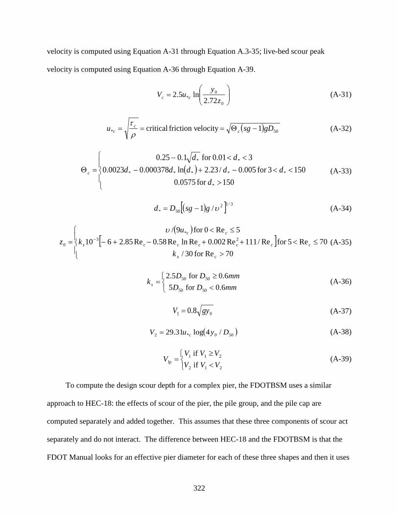
322

velocity is computed using Equation A-31 through Equation A.3-35; live-bed scour peak

velocity is computed using Equation A-36 through Equation A-39.

=

0

0* 72.2

ln5.2z

yuV cc (A-31)

( ) 50* 1elocityfriction v critical gDsgu cc

c −Θ===ρ

τ (A-32)

( )

><<−+−

<<−=Θ

150for 0575.01503for 005.0/23.2ln000378.00023.0

301.0for 1.025.0

*

*****

**

dddddd

dd

c (A-33)

( )[ ] 3/1250* /1 υgsgDd −= (A-34)

( )

[ ]

>≤<++−+−

≤<= −

70Refor 30/70Re5for Re/111Re002.0RelnRe58.0Re85.2610

5Re0for 9/23

*

0

cx

ccccccs

cc

kk

uz

υ (A-35)

<≥

=mmDDmmDD

ks 6.0for 56.0for 5.2

5050

5050 (A-36)

01 8.0 gyV = (A-37)

( )500*2 /4log31.29 DyuV c= (A-38)

<≥

=212

211

if if

VVVVVV

Vlp (A-39)

To compute the design scour depth for a complex pier, the FDOTBSM uses a similar

approach to HEC-18: the effects of scour of the pier, the pile group, and the pile cap are

computed separately and added together. This assumes that these three components of scour act

separately and do not interact. The difference between HEC-18 and the FDOTBSM is that the

FDOT Manual looks for an effective pier diameter for each of these three shapes and then it uses

323

this diameter to compute the scour depth. Conversely, HEC-18 applies a correction factor, Kx to

the scour parameter instead of the effective diameter parameter.

Explicitly, the total scour of a complex pier in the FDOTBSM is computed by:

****pgpccol DDDD ++= (A-40)

To compute the effective column (pier) diameter, Equation A-41 through Equation A-46 are

used:

1yH

for 0

10for 2476.03617.01162.0

0(max)

col

(max)0(max)0

2

(max)0*

>

≤≤

+

−

= yH

yH

yH

bKKKD

colcolcolcolfs

col

α

(A-41)

<≥

=col

colcol

byybyb

y5for 5for 5

00

0(max)0 (A-42)

−+= columnsr rectangulafor 4180

97.086.0

columnscircular for 14ππα o

sK (A-43)

col

colcol

blb

Kαα

αsincos +

= (A-44)

>+

≤+

=o

o

ff

ff

f45for

43

45for 4

3

12

21

α

α (A-45)

>

≤

+

+

−

=

3for 0

3bffor 103.012.0.col

2

col

colcolf

bfb

fb

f

K (A-46)

324

To illustrate bcol, the column width, and f, the side overhangs, a definition sketch has been

provided (Figure A-12). To compute the effective pier diameter of the pile cap, Equation A-47 is

used:

+

−−=

5.0

(max)0(max)0

* 695.1exp77.104.1expy

Ty

HbKKD pc

pcspc α (A-47)

where Ka is the same as it was when it was computed for a column except that the pile cap’s b is

used instead of the column’s b; Ks is the same as for a column; y0(max) is computed using

Equation A-48:

( )[ ] ( )[ ]

( )[ ]

<

<=

72

5.20 0

72

5.20

7.25.2

(max)0

64.1for

64.1for 64.1

pcx

pcxpcx

bKTyy

bKTybKTy (A-48)

To compute the effective pier diameter for the pile group, Equation A-49 through Equation A-55

are used:

psmhsppg WKKKKD =* (A-49)

( ))()()()()(

910

9 pilegroupspilespilespilegroupspiles

s KKKbsKK

K −−+

−

= (A-50)

−+=

groups piler rectangulaor piles squarefor 4180

97.086.0

arrays group pileor pilescircular for 14

group) pileor pile( ππαsK (A-51)

−

−−= 6.0

111341

pi

p

pisp

wsW

wK (A-52)

325

>><

≤<+=

5,15&5,19.1

5&5,96.0045.0

αα

αm

mmK m (A-53)

>≤

=msppsmspps

mspps

KKWKyKKWKKKWKyy

y2,2

2,

0

00(max)0 (A-54)

>≤

<≤

≤≤

=

10for 1

00for 0

10for 8.0tanh5.1

(max)0

(max)0

(max)0(max)0

yH

yH

yH

yH

K

pg

pg

pgpg

h (A-55)

2.2.2.4 FDOTBSM: brief discussion

As briefly mentioned in Section A.3.1, these series of equations have been the most

successful equations for predicting bridge pier scour depths (Figure A-13). The equations in the

FDOT Bridge Scour Manual are considered by many to be the state of the art with the regard to

predicting scour depths for a cohesionless sediment. They appear to provide excellent results,

and although they are somewhat complicated, they are easily programmed into a computerized

algorithm. Unfortunately, the FDOTBSM does not give any recommendations as far as

designing scour depths for rock or cohesive sediments. Therefore, an engineer has no choice but

to refer back to HEC-18 for guidelines when designing for these bed materials.

326

Table A-1. Values for k1 V*/ω k1 Mode of Bed Transport

<0.50 0.59 Mostly contact bed material discharge

0.50 to 2.0 0.64 Some suspended bed material discharge

>2.0 0.69 Mostly suspended bed material discharge

Adapted from Richardson, E. V. and Davis, S. R. (2001). “Evaluating scour at bridges fourth edition.” Publication No. FHWA NHI 01-001 hydraulic engineering circular no. 18. http://isddc.dot.gov/OLPFiles/FHWA/010590.pdf, Sept. 2, 2008. Table A-2. Pier Nose Shape Correction Factors

Correction Factor K1 For Pier Nose Shape

Shape of Pier Nose K1

(a) Square nose 1.1

(b) Round nose 1.0

(c) Circular nose 1.0

(d) Group of cylinders 1.0

(e) Sharp nose 0.9

Adapted from Richardson, E. V. and Davis, S. R. (2001). “Evaluating scour at bridges fourth edition.” Publication No. FHWA NHI 01-001 hydraulic engineering circular no. 18. http://isddc.dot.gov/OLPFiles/FHWA/010590.pdf, Sept. 2, 2008.

327

Table A-3. Bed Condition Correction Factors

Increase in Equilibrium Pier Scour Depths, K3, for Bed Condition

Bed Condition Dune Height (m) K3

Clear-water scour N/A 1.1

Plane bed and antidune flow N/A 1.1

Small dunes 3 > H ≥ 0.6 1.1

Medium dunes 9 > H ≥ 3 1.2 to 1.1

Large dunes H ≥ 9 1.3

Adapted from Richardson, E. V. and Davis, S. R. (2001). “Evaluating scour at bridges fourth edition.” Publication No. FHWA NHI 01-001 hydraulic engineering circular no. 18. http://isddc.dot.gov/OLPFiles/FHWA/010590.pdf, Sept. 2, 2008.

Figure A-1. Shields Diagram [Adapted from Lemke, K. A. (2010). “Stream sediment.” University of Wisconsin-Stevens Point, http://www.uwsp.edu/geo/faculty/lemke/ geomorphology/lecture_outlines/03_stream_sediment.html, Sept. 14, 2010.]

328

Figure A-2. Fall Velocity vs. Grain Size [Adapted from Richardson, E. V. and Davis, S. R. (2001). “Evaluating scour at bridges fourth edition.” Publication No. FHWA NHI 01-001 hydraulic engineering circular no. 18. http://isddc.dot.gov/OLPFiles/ FHWA/010590.pdf, Sept. 2, 2008.]

Figure A-3. Common Pier Shapes [Adapted from Richardson, E. V. and Davis, S. R. (2001). “Evaluating scour at bridges fourth edition.” Publication No. FHWA NHI 01-001 hydraulic engineering circular no. 18. http://isddc.dot.gov/OLPFiles/ FHWA/010590.pdf, Sept. 2, 2008.]

329

Figure A-4. Diagram used to determine Khpier [Adapted from Richardson, E. V. and Davis, S. R. (2001). “Evaluating scour at bridges fourth edition.” Publication No. FHWA NHI 01-001 hydraulic engineering circular no. 18. http://isddc.dot.gov/OLPFiles/ FHWA/010590.pdf, Sept. 2, 2008.]

Figure A-5. Diagram used to determine a*pc [Adapted from Richardson, E. V. and Davis, S. R.

(2001). “Evaluating scour at bridges fourth edition.” Publication No. FHWA NHI 01-001 hydraulic engineering circular no. 18. http://isddc.dot.gov/OLPFiles/ FHWA/010590.pdf, Sept. 2, 2008.]

330

Figure A-6. Illustration sketch for computing scour when a pile cap is above the bed [Adapted from Richardson, E. V. and Davis, S. R. (2001). “Evaluating scour at bridges fourth edition.” Publication No. FHWA NHI 01-001 hydraulic engineering circular no. 18. http://isddc.dot.gov/OLPFiles/ FHWA/010590.pdf, Sept. 2, 2008.]

Figure A-7. Diagram for computation of correction factor, Km [Adapted from Richardson, E. V. and Davis, S. R. (2001). “Evaluating scour at bridges fourth edition.” Publication No. FHWA NHI 01-001 hydraulic engineering circular no. 18. http://isddc.dot.gov/OLPFiles/ FHWA/010590.pdf, Sept. 2, 2008.]

331

Figure A-8. Diagrams used to illustrate computation of equivalent pier width [Adapted from Richardson, E. V. and Davis, S. R. (2001). “Evaluating scour at bridges fourth edition.” Publication No. FHWA NHI 01-001 hydraulic engineering circular no. 18. http://isddc.dot.gov/OLPFiles/ FHWA/010590.pdf, Sept. 2, 2008.]

Figure A-9. Diagram used to compute the spacing coefficient, Ksp [Adapted from Richardson, E. V. and Davis, S. R. (2001). “Evaluating scour at bridges fourth edition.” Publication No. FHWA NHI 01-001 hydraulic engineering circular no. 18. http://isddc.dot.gov/OLPFiles/ FHWA/010590.pdf, Sept. 2, 2008.]

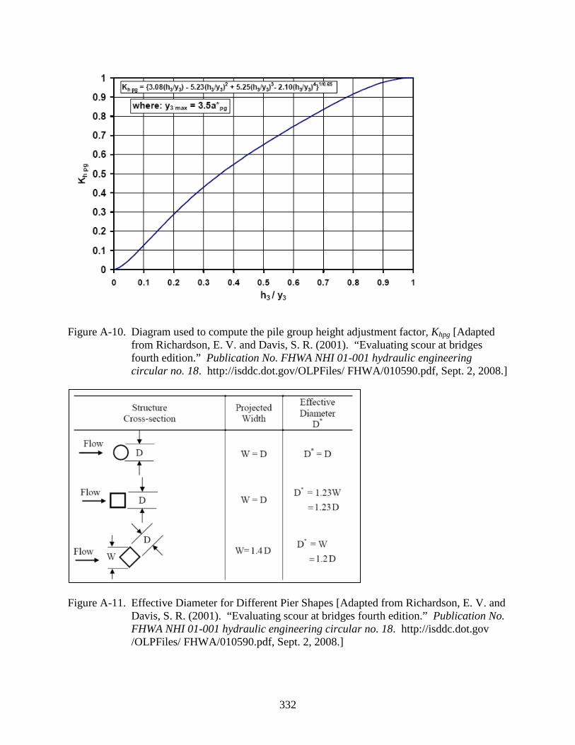
332

Figure A-10. Diagram used to compute the pile group height adjustment factor, Khpg [Adapted from Richardson, E. V. and Davis, S. R. (2001). “Evaluating scour at bridges fourth edition.” Publication No. FHWA NHI 01-001 hydraulic engineering circular no. 18. http://isddc.dot.gov/OLPFiles/ FHWA/010590.pdf, Sept. 2, 2008.]

Figure A-11. Effective Diameter for Different Pier Shapes [Adapted from Richardson, E. V. and Davis, S. R. (2001). “Evaluating scour at bridges fourth edition.” Publication No. FHWA NHI 01-001 hydraulic engineering circular no. 18. http://isddc.dot.gov /OLPFiles/ FHWA/010590.pdf, Sept. 2, 2008.]

333

Figure A-12. Definition Sketch for Scour Around a Complex Pier [Adapted from Richardson, E. V. and Davis, S. R. (2001). “Evaluating scour at bridges fourth edition.” Publication No. FHWA NHI 01-001 hydraulic engineering circular no. 18. http://isddc.dot.gov /OLPFiles/ FHWA/010590.pdf, Sept. 2, 2008.]

Figure A-13. Measured vs. computed scour depths [Adapted from “Florida department of transportation bridge scour manual (2005).” <http://www.dot.state.fl.us/ rddesign/dr/Bridgescour/FDOT-Scour-Manual-6-2-2005-Final.pdf>, Sept. 2, 2008.]

334

APPENDIX B FLORIDA METHOD FOR SERF TESTS

B.1 New Operating Procedure for SERF

Because of the overhaul of the SERF, a new operating procedure for tests needed to be

developed. When conducting a test, there are three possible things that can be tested, and each of

these three tests has its own procedure:

• Shear stress for a specified sample • Critical shear stress for a specified sample • Erosion rate for a specified sample

Please note that although it is possible to measure shear stresses and erosion rates at the

same time (the computer code has been developed), it may be inaccurate. Shear stresses should

only be measured concurrently with erosion rates when a flat disk is installed in the shear stress

sensor or when a sample is smooth enough to be considered “flat.” Generally, as per the

discussion in Chapter 4, if median size of eroding elements is expected to be greater than 0.5

mm, an eroding section is not considered “flat” and it probably will affect the velocity profile

downstream from it. Because of the positioning of the shear sensor, this disturbance in velocity

profile will probably affect the erosion rate of the sample. If/when it becomes possible to

measure velocity profiles in the SERF (Chapter 8), it may be possible to justify measuring shear

stress and erosion rates at the same time, but until that happens, the eroding material should not

be considered to be “flat.” Procedure for the testing erosion rate includes a section on

concurrently measuring shear stress, but keep this disclaimer in mind when running future tests.

B.2 Preliminary Procedure for Tests

Before any of the three categories of tests are set up, a few preliminary steps need to be

completed. First, the SERF operator needs to decide what conditions are going to be run.

Because of sand recirculating issues, the sand injector has not been installed. When installed, the

335

sand injector will warrant its own set-up procedure, but currently the only decision for an

operator is whether or not to install the vortex generator.

B.2.1 Vortex Generator

To install/remove the vortex generator, the following procedure needs to be conducted:

1. If vortex bar is already installed and it needs to be removed, push the bar through the flume and install the vortex generator plugs.

2. If the vortex bar needs to be installed, remove the vortex generator plugs from the SERF, and slide the bar into the flume. Make sure the O-rings remain on (they prevent leakage).

B.2.2 Temperature Control and Filtering

To insure temperature control during tests, the temperature control-filter system needs to

be turned on, but first it needs to be primed. To do this:

1. Open the air release valve on the filter (Figure B-1).

2. Open the PVC release valve in the filter-chiller system (Figure B-2).

3. Push the plunger on the PVC slide valve down (Figure B-3). This causes the filter to run in reverse and fills it with water.

4. Turn on the pool pump using the white switch (circled in Figure B-4).

When water begins to shoot out of the air release valve, close the air release valve.

5. Turn the pool pump off.

6. Pull the slide valve up to the “filter” position (Figure B-5). Turn to lock it into place.

7. Turn the pool pump back on. The filter is now primed and running. Pressure in the filter should be approximately 25 psi. If pressure is much higher than 25 psi, the filter needs to be backwashed. To backwash the filter, fill the reservoir tank with water and run the filter in reverse until approximately 700 gallons of water remain in the reservoir tank. Make sure the PVC valve in (2) is open. If it remains closed, a pipe will burst because pressure inside the filter-chiller system will build. This may irreparably damage the water chiller. Once drainage water is clear, the filter has been properly backwashed. Then, refill the reservoir tank and resume with instructions below.

8. Turn on the water chiller (Figure B-6). Pressure in the system should drop to approximately 20 psi. Now, water is being cooled and filtered (somewhat as discussed in Chapter 7 and Chapter 8).

336

9. Turn the thermostat on the back side of the water chiller to the desired temperature (Figure B-7).

10. The temperature control-filter system is now working. Leave this system on during tests.

B.3 Stand-Alone Shear Stress Test

As discussed in Chapter 4, during a shear stress test, the goal is to find how the roughness

of a soil or rock sample affects the wall shear stresses along its face. Please note that a shear

stress test on an existing sample will disturb it; this is a disadvantage to the testing method, but at

present, there is no way to accurately measure shear stress and avoid this. If multiple Shelby

tubes are taken, it may be advantageous to dry one, sieve it, mix thoroughly (assuming

uniformity) and use the procedures for conducting a synthetic test. If gradation is present, each

graded section could be dried and mixed separately to produce multiple test discs using the

synthetic method. These procedures assume a uniform sample. The procedure for a shear stress

test is as follows:

1. Prepare the test disk. Because the shear sensor has a removable circular disk (Figure B-8), this disk can be replaced with a disk of the appropriate roughness for use in shear stress testing.

a. For a synthetic sample, disk preparation is easy.

i. A uniformly, evenly mixed batch of aggregate used to make the sample synthetic sample should be set aside.

ii. A 50 mm acrylic disk should be coated with epoxy. Experience has shown that JB Weld two-part epoxy (Figure B-9) works the most effectively. Be sure to spread the epoxy evenly and level.

iii. Press the epoxy coated disk onto a random portion of the aggregate so that the disk coats with sediment particles.

iv. Multiple disks should be prepared to ensure that a true random sampling form the aggregate is achieved (Figure 3-10).

b. For a non-synthetic non-rock sample, disk preparation is similar

i. A 50 mm acrylic disk should be coated with epoxy.

337

ii. Press the epoxy coated disk onto the top of the Shelby tube so that aggregate from the Shelby tube sample coats the disk.

iii. If multiple Shelby tubes are collected, multiple disks should be prepared.

c. For a rock core, disk preparation is the most complicated.

i. A sliver of the top of the rock core needs to be cut from it. The sliver must remain intact and it must be no more than 1cm thick. The sliver must be flat on both its top and the bottom.

ii. The rock core sliver needs to be carefully epoxied to a 50mm plastic disk.

iii. A hole needs to be carefully drilled through its center, and the entire rock core sliver-disc apparatus needs to be milled to 50 mm in diameter.

2. Open the shear stress sensor’s access hatch (Figure B-11) and remove the existing plastic disc. Attach the newly prepared disk using the screw through the center of the disc (Figure B-12).

3. Close the SERF access hatch by using an Allen wrench to tighten the 8 hex-screws on top of the flume. Make sure the black rubber gasket is between the access hatch cap and the top of the flume. DO NOT OVER-TIGHTEN. The screw threads that attach the access hatch to the flume are drilled directly into the aluminum and if they are over-tightened, they will strip.

4. Check the shear sensor access window for pollution. Often, particles get stuck in the wet section of the shear sensor, and they can block the space between the Servo magnet and the Hall Sensor.

5. If the wet section of the shear sensor is polluted, remove the Plexiglass window and clean it. If not, proceed to step 6.

6. Calibrate the shear stress sensor.

a. Zero the sensor using the knobs (1) and (2) as shown in Figure B-13. The coarse adjustment knob is knob (2) and the find adjustment knob is knob (1). When the sensor is properly zeroed, the ammeter on the front of the amplifier should read 0.

b. Press and hold the CAL button on the shear stress sensor (4). This sends a voltage to the calibration solenoid based on the position of knob (5), which causes the deflection solenoid to react. Turn knob (3) such that the ammeter on the amplifier deflects to the corresponding correct stress reading. For example, if knob (5) is turned to 50, the corresponding stress read on the ammeter should be 50 Pa. Release the CAL button (4). Repeat for several values of (5) to make sure the sensor is working. Note that the shear sensor runs at 4 different ranges: 10 Pa, 20 Pa, 50 Pa, and 100 Pa. To set the range of the sensor, turn knob (6). Keep in mind that if the range is set to anything less than 100 Pa, a calibration voltage of

338

100 Pa will rail the instrument. Likewise, if the range is 20 Pa a calibration voltage of 50 Pa will do the same thing. When the range goes below 100 Pa, the scale on the ammeter adjusts accordingly. Therefore, a calibration voltage of 50 Pa when the range is on 50 Pa will still deflect the ammeter to full deflection (this is correct and it is how the instrument was designed).

7. If the shear sensor does not calibrate, there must be something incorrect with the mechanical setup of the sensor. Mechanical issues with the shear sensor are common, and they must be addressed before a shear test can commence.

a. The most common mechanical issue with the shear sensor is pollution (see step 5). First, recheck to make sure the gap between the Servo magnet and the Hall Sensor is present. If not, re-clean and recalibrate.

b. If the gap between magnet and sensor is present, the next most common mechanical issue is the connection between the deflection magnet and the platform. Open the round upstream access hatch on the left side of the sensor as the sensor is observed from the middle of Reed Lab (Figure B-14).

c. When looking into the round hole in the sensor, there should be a small gap between the magnet battery and the solenoid. When the connection slips, an illustration as shown in Figure B-15 is what will be seen instead.

d. If it looks as though the magnet battery is rubbing against the deflection solenoid as shown in this figure, loosen the screw shown in Figure B-16 and reposition the brass rod so that there is an air gap present between the deflection solenoid and the magnet battery.

Try to recalibrate the sensor. If it still does not work, remove the brass rod and magnet battery completely and check to make sure the connection between the magnet and the brass rod is not broken (it often breaks). Reattach using a two-part plastic super glue. DO NOT USE METAL EPOXY SUCH AS JB WELD. IT WILL CAUSE AN ERROR IN THE SOLENOID BECAUSE JB WELD IS MAGNETIC.

e. If the sensor will still not calibrate, repeat steps i. – v. with the calibration solenoid (although this breaks much less often).

f. This should fix the sensor. The only other possible explanation could be that the leaf springs have become permanently deformed and they need to be replaced (contact Raf Crowley for procedure on how to do that) or water has leaked into the dry portion of the sensor.

g. If leakage is suspected at any time when using the shear sensor, open the panel exposing the electronics (Figure B-17), UNPLUG THE SENSOR, and assess the damage. The sensor may need to be resealed and/or IC’s may need to be replaced. Usually though, if the sensor is given time to dry out, it will begin working again.

339

h. If these troubleshooting procedures do not work, contact Raf Crowley ([email protected]) or Hans Prechtel ([email protected]). If these procedures have made the sensor work properly, the SERF is now ready for shear stress testing.

8. Turn on the computer in the SERF control room and start the vi labeled Flume Control No Motor. The shortcut for this vi is located on the desktop in a folder called “Flume Shortcuts.” If the correct vi has been opened, its front panel should look like Figure B-18.

9. Make sure that the data range in the Labview program matches the data range on the shear stress sensor amplifier (Figure B-19)

10. Turn the pump on and make sure that the digital display reads “remote.” Press forward on the digital pump readout (this initializes the pump).

11. Press start in Labview, and the Labview program should ask where to save the data file. Files are saved as .dat files to allow for easy Matlab data analysis, but this can be changed to .xls format if the operator feels more comfortable using Excel. Directions on how to do this are in Appendix C.

12. Press record on the DVR.

13. Adjust the pump speed to approximately 20 Hz. This will start a flow of water through the flume and pressurize it. Anything less than 20 Hz is not high enough to overcome the head differential between the flume and the reservoir tank. Allow the flume to run for a few seconds until bubbles in the flume are eliminated.

14. If pressure transducers are to be used during the shear test, next they need to be “bled.” To bleed a pressure transducer, unplug both tubes from the flume to the transducer. Make sure to unplug the downstream tube first. The transducers are designed to tolerate over pressurization on the positive side only. Because the flume should be running at approximately 20 Hz, when the tubes are unplugged, water should be going into them. Lightly tap on the tubes to eliminate bubbles from them. When bubbles have been eliminated, plug the tubes back into the sensor. Plug the upstream side in first this time, then the downstream side.

15. While bleeding the sensors, real-time graphs should have begun to be generated in the Labview program. As far as data collection goes, these graphs are meaningless. They were included in the program for the user to get a broad idea of shear stress/pressure conditions, but they are sampled at a much lower frequency than data collection.

16. Now, everything is ready for data collection. Bring the pump to the desired flow speed. Give the system a few seconds to stabilize. Stabilization is achieved when the shear sensor begins to display a somewhat consistent shear stress from the graphs.

17. When conditions have stabilized, press the “RUN” button in Labview. This will stop the generation of the graphs (but this is OK) for a length of time that is dependent on the Sampling Rate Parameter (default is 1 kHz) and the Number of Samples Parameter

340

(default is 10,000). Both these values can be changed as the Labview program runs to allow for different sampling frequencies and different sampling lengths. A long sampling length though means lots of computer memory. Anything over 15,000 data points should not be used because the computer does not have enough RAM to support this (the computer only has 3.5 GB).

18. When the graphs start moving again, data collection has been completed. Bring the pump to the next desired flow rate, wait for it to stabilize, hit the run button to collect data, repeat.

19. Repeat for flow rates that are to be investigated.

20. When testing is done, gradually bring the pump speed down to zero. For example, if a pump frequency of 30 Hz was used for the test, bring the pump down to 25 Hz, let it run for 5 seconds, then bring it to 20 Hz, let it run for 5 seconds, etc. the way to 0 Hz pump frequency. This gradual velocity reduction allows the shear sensor to “catch up” with changing flow conditions and can help prevent breakage to the instrument.

21. The test may now be repeated, or a new sample disk may be installed. It is recommended to repeat each test at least three times and to recalibrate the shear sensor after every test. Before removing the access hatch to install a new sample, make sure the valves on the pressure transducer are closed. When the access hatch is removed, water rushes from the flume into the reservoir because of the pressure differential created by exposing the flume to air. If the pressure transducer valves are open, there is a significant risk of breaking one or both of the transducers.

22. Go to the saved .dat files and perform data analysis. The most effective method for data analysis is Matlab, and there are several Matlab algorithms written in the G:\analysis folder that average samples over the entire sampling domain, perform spectral analyses, plot graphs of the results, etc. Excel can be used, but every data run has 10,000+ data points per flow rate and an Excel analysis will be arduous. SERF operators are encouraged to learn Matlab.

B.4 Critical Shear Stress Test in SERF

Shear stress tests should be conducted first on any sample batch so that a correlation can be

developed between flow rate and shear stress. Once a shear stress analysis has been completed, a

critical shear stress test may be performed:

1. Make sure that a flat disk has been installed in the shear stress sensor. Alternatively, the entire shear sensor may be removed and the shear sensor plug (Figure B-20) can be installed in its place.

2. To remove the shear sensor, loosen ONLY the hex screw on the sensor flange (Figure B-20).

341

3. Once the hex screw loosened, carefully pull and twist the sensor to release the shear sensor from its blue Loctite bond.

4. Coat the sensor plug (Figure B-21) with blue Loctite, and slide it into the sensor hole. Make sure the plug is level with the flume bottom.

5. Retighten the hex screw.

6. If the sensor plug is not installed, the shear sensor still needs to be turned on during shear stress tests. The magnets in the sensor help to prevent the sensor disc from moving, and turning the sensor on will help to prevent damage to the sensor and help to prevent flow disturbances in the SERF.

7. Load the test section of rock core, Shelby tube, or synthetic material into the piston-cylinder apparatus (Figure B-22). Grease the piston-cylinder’s O-rings with a silicon grease.

8. Attach the piston to the Servo motor’s feedscrew using a screw.

9. Raise the Servo motor (which is now attached to the piston and the cylinder) into the SERF’s sample hole. Make sure to put an O-ring around the top of the cylinder to prevent leakage. If using an opaque piston, also make sure that the ridges on the top of the cylinder provide a clear line of sight for the lasers (Figure B-23).

10. Attach the four threaded rods around the cylinder to the bottom of the SERF.

11. Tighten the compression coupling around the bottom of the test cylinder through the threaded rods. DO NOT OVER TIGHTEN AS IT WILL CAUSE THE TEST CYLINDER TO CRACK. If leaks develop, the compression screws can be retightened. When installed, the apparatus should look like Figure B-24.

12. If lasers are to be used, turn on the lasers by clicking the “on” button on the surge protector shown in Figure B-25.

13. Open the program labeled “Motor Mover.” The front panel is shown in Figure B-26.

14. Flip the input switch on the VGA-BNC adapter so that the right monitor of the control program is looking into the flume. Tune to channel 2 on the DVR to see the eroding test section.

15. Turn on the motor by flipping the switch on the black box below the laser amplifiers and start the motor mover program. Click start on the Motor Mover program.

16. Move the motor up in small increments until the control boxed from the lasers indicate that they are blocked. The control boxes will “click” when they are blocked and the lights on the amplifiers will switch off. A “small increment” is approximately 500 steps in the motor mover program. DO NOT MOVE THE MOTOR MORE THAN 5,000 STEPS AT A TIME. It will cause the motor’s gears to grind and may cause the motor to break.

342

17. Once the control boxes have clicked and the lasers indicate that the sample is level with the flume bottom, verify that the flume is level visually by looking at the right monitor on the SERF computer. If the sample is level, proceed. If not, re-level.

18. Open the program labeled “Pump Control” from the “Flume Control Shortcuts” folder on the desktop Press the start button. The front panel is shown in Figure B-27.

19. Click Start the pump at approximately 20 Hz to pressurize the flume. If dealing with a highly erodible material, this can be rather tricky. The flume will need to be pressurized, then the motor will need to re-level the sample using the same procedure outlined in (11).

20. Bring the pump down to a slow flow speed (approximately 5 Hz).


22. Slowly increase the pump speed in small increments (approximately 0.25 Hz) and watch the right monitor. Look for any particle motion along the bed.

23. When incipient motion is detected, stop the pump and record the flow rate. The critical velocity for the material just tested in now known.

24. Use correlations developed in shear stress testing to convert critical flume velocity to critical flume shear stress. Now, the critical shear stress for the material is known and the critical shear stress test has been completed.

25. Repeat the critical shear stress test at least three times for each material.

B.5 Erosion Rate Test

The erosion rate test is the most complicated test that can be conducted in the SERF. To

reiterate, until velocity profiles can be measured in the flume, shear stress tests and erosion rate

tests should be conducted independently. Once velocity profiles can be measured, it may be

possible to justify running both sets of tests concurrently, but until then, it is believed that

placing a rough sample upstream from an eroding sample will affect the hydrodynamics

downstream from the rough sample and alter the measured erosion rate of the bed material. To

conduct the erosion rate test:

1. Load a sample into the piston-cylinder using the same steps for a critical shear test.

2. Install the flat disc into the shear stress sensor, or install the shear sensor plug. If the sensor is to remain in the flume, follow plug installation steps from the critical shear stress test.

343

3. Turn on the motor.

4. Turn on the lasers and level the sample using the same techniques used for an erosion rate test. Note that by default the lasers use “and” logic to advance the sample. If an operator feels that “or” logic is more appropriate, refer to Appendix C for guidelines on how to change this.

5. Open the pump control program.

6. Fill and pressurize the flume. If pressure drops are to be measured, bleed the pressure transducers using the same method used for a critical shear stress test.

7. Stop the pump. If shear stresses are to be measured, calibrate the shear sensor using the same method used for a shear stress test.

8. Turn the pump on a low flow rate (~5 Hz). This will help to push bubbles away from the SEATEK during SEATEK calibration. If the SEATEK is not to be used, skip steps 9-15 and go straight to step 16.

9. Open TeraTerminal. TeraTerminal is sort of like a Windows 7 version of HyperTerminal (which is what Slagle and Trammel used to control the SEATEK when it was first turned on). The TeraTerminal shortcut is on the Windows 7 control bar at the bottom of the screen, next to the Labview 2009 shortcut (Figure B-28).

10. In TeraTerminal, click the option to read from the Serial Port.

11. Turn on the SEATEK. In TeraTerminal, output should read MTAS V3.12S Input Command [? For help].

12. Pressing “?” will give a list of SEATEK commands. The important parameters to change in the SEATEK are temperature (TE), maximum transducer depth (MA), threshold voltage (V), and number of sample runs (N).

13. First, change the temperature to the correct temperature. For example, to change the temperature to 21oC, type “TE 21” and Enter.

14. Next, press “P” to ping the SEATEK sensors. If the depth readings that are returned are around 4.92 cm, the SEATEK is working properly. If not, play with the “MA” and “V” commands until the proper depths are being returned. There are 12 crystals in the SEATEK array – 8 within the sample’s area and 4 along its outside. The crystals that are most important are the first 8 as they measure the sample position. The outside 4 crystals measure the depth to the solid flume bottom (4.92 cm). Please note that when this project began, crystal #2, crystal #5, crystal #6, and crystal #10 were damaged; as of 2007, they were not working properly (this will be addressed in Labview).

15. Keep pinging the crystals after each “MA” and “V” command to determine if they are working properly.

344

16. Once it the crystals are working properly, set up a data run to confirm that the crystals can read multiple results correctly. Take at least twenty readings by executing the following commands:

a. N 20; Enter

b. D; Enter

17. Exit TeraTerminal. The serial port on any computer can only communicate with one program at a time, and if TeraTerminal is left open, Labview will not read from the Serial port because TeraTerminal already is doing so.

18. Open the Labview vi entitled “Flume Control With Motor (With Temperature Patch).” Its front panel should look like Figure B-29.

19. If the SEATEK is not to be used, turn it off using the switch on the control panel.

20. If the lasers are not to be used, turn them off using the switch on the control panel.

21. Assuming the SEATEK is to be used, from the TeraTerminal procedures, turn off the crystals that are not working properly by clicking on the green LED lights on the Labview front panel. Note that crystals 8-12 are not listed. The malfunctioning crystal, crystal #10 is automatically eliminated from consideration during data processing (Appendix C).

22. Make sure the motor is turned on in the front panel.

23. Press start on the Labview program. Two output files will be generated – one for analog signals (shear stress, pressure, temperature, flume speed, time) and the other for digital data (time, number of steps, motor position). Save these files in the appropriate directory.

24. Move the pump control to the desired flow speed.


26. The test should now be running. Keep an eye on it for approximately 20 minutes to make sure everything is working properly. If a crystal begins to malfunction, it can be turned off in the middle of a data run. If the SEATEK overall or the lasers begin to malfunction or give nonsensical results (for example, the SEATEK when some clays are used), they can be turned off as well.

27. If two pumps are to be used during the test, turn on the “2nd Pump” switch. This will insure that the correct velocities are recorded in the analog output file.

28. If analog signals are to be recorded (shear stress and pressure drop), the program will run much like it did for shear stress tests. Water will flow through the flume, graphs will generate on the front panel, and every specified time step (the default is 10 minutes, but this can be changed – see Appendix C), the graphs will freeze and analog output files will be written at the specified frequency.

345

29. If analog signals are not to be recorded, skip step 29. Motor position will be recorded every time the program goes through its loop (see Appendix C) in the digital output file.

30. Allow the SERF to run for the specified length of time. It should be monitored during operation to insure that nothing malfunctions, but once it has been set up, it should work properly.

B.6 Remote SERF Operation

In any SERF test, it is now possible to control the flume remotely if required hard switches

have been turned on. This is especially useful in monitoring erosion-rate tests because erosion

rate tests often need to run for 24 hours or more. Tests do not need to be constantly monitored,

but they do require someone to look at them from time to time to make sure they are running

correctly. Remote operation also useful for changing flow parameters during a test. If one of

these scheduled modifications needs to be made late at night or early in the morning, remote

operation is convenient.

The worst thing that can happen during a SERF test is the motor can malfunction due to

bad readings from the SEATEK or lasers. Sometimes, the motor may retract such that the piston

pulls out of the test cylinder. If this happens, the lab can flood. Other times, the motor may

advance uncontrollably and cause the sample to be pushed up to the top of the flume. If either of

these things happens, the test needs to be stopped, the source of error needs to be assessed and

addressed so that nothing malfunctions again. Software limit switches have been installed in

MAX (Measurement and Automation Explorer), and the lab has yet to flood, but there is no

hard-wired method installed to prevent uncontrolled advancement/retraction. Therefore,

operators need to be conscious of this risk. Although most bugs from operation have been

worked out, operators are still encouraged to monitor testing as much as possible.

346

B.6.1 Remote Visual Inspection

The easiest way to monitor a SERF test is visually. Two cameras look at the important

parts of the flume (the eroding test section and the shear stress sensor), and visual data from

these cameras is useful at determining whether or not a test is running correctly. A third camera

is set up to monitor the entire lab from above so that a remote operator can have even more

information with how a test is going in the device.

Visual inspection is conducted by using the DVR because the DVR has networking

capabilities. To see what is being recorded in the DVR and to control the DVR remotely, the

following procedure should be followed:

1. Initiate a Virtual Private Network (VPN) connection with the UF network. The DVR and SERF can only be accessed through a VPN because when remote operation was set up, there were concerns about providing security for it. The VPN allows for security options that are not possible through a normal network connection. To set up a VPN connection for the first time, follow the UF guidelines for VPN. They can be accessed at http://net-services.ufl.edu/provided_services/vpn/vpn-install.html.

2. Open Microsoft Internet Explorer. Remote operation of the DVR will not work with Mozilla Firefox. This technique has not been tested with Apple Safari or Google Chrome, but it may work.

3. In the address bar of Internet Explorer, type the static IP address for the DVR – http://10.5.72.138. Press Enter.

4. A popup will appear that asks for a username and password. The username is “admin” and the password is also “admin.”

5. A window should appear that looks like Figure B-30. If this window is generated, remote operation has been initialized properly and the DVR can be viewed and operated from Internet Explorer.

B.6.2 Remote Labview Operation

If after visual inspection, an operator realizes that a test needs to be shut down or if an

operator wishes to monitor data collection and Labview operation remotely, the SERF computer

347

has also been configured to do this. The following procedure is used for remote control of the

computer:

1. Initialize a VPN connection to the UF network.

2. Open Windows Remote Desktop Software. This capability is standard in Windows XP, Windows Vista, and Windows 7. Once open, the remote desktop software looks like Figure B-31.

3. Go back to the remote desktop connection software. Next to “Computer,” type the name of the computer. The computer’s name is “KEYWEST.”

4. Press connect.

5. The computer will ask for a username and password. Type the correct username and password for the computer.

6. Remote desktop connection is now complete. The computer is now being controlled remotely. While remote control is taking place, the computer will lock itself.

B.7 SERF Operation Troubleshooting

Although most bugs have been worked out, there are some common errors associated with

SERF operation. Problems with the shear stress sensor are the most common and they have

already been discussed. The next largest issue with operation is the development of leaks around

the test cylinder. Leaks tend to emanate from two sources – from the piston and from the

cylinder-flume connection. Fixing the latter is easy. If water is leaking from the cylinder-flume

connection, the compression screws on the bottom of the cylinder need to be tightened until the

leak stops. Fixing leaks around the piston are much more difficult. Piston leaks develop because

the piston’s O-rings were not properly cleaned when the sample was loaded. Often, pieces of

debris, sediment, or grit will get stuck in between the space between the O-ring and the inner

cylinder wall. Eventually, a leak will develop and it needs to be addressed. Unfortunately, the

only way to address these leaks is to stop the test, remove the cylinder, remove the piston,

348

remove the O-rings, clean the O-rings, re-grease them, and start the test again. As seen then, it is

vitally important to make sure that O-rings are properly cleaned before initializing a test.

Leaks due to motor retraction were already discussed in the erosion rate test section of this

appendix. The most effective method for preventing these leaks is to monitor the test as much as

possible (remote access makes this easier). Visual data analysis, even from afar, will show if the

gears are grinding. If SEATEK data is coming back badly or if a many negative steps are being

recorded in the Labview program, a remote operator can be sure that gears are grinding. Visual

inspection too will show that the sample is not level with the flume bottom. This can only mean

that the piston/sample is too low and that the motor has retracted too much.

Other problems in the SERF are much less common, and they will not be discussed further.

If a problem comes up that a novice operator cannot solve, Raf Crowley should be contacted

([email protected]) so that he can help to troubleshoot.

349

Figure B-1. Air Release Valve on Sand Filter

Figure B-2. PVC release valve for Chiller-Filter System

350

Figure B-3. Slide Valve in the Down Position

Figure B-4. Pool Pump Switch

351

Figure B-5. PVC Slide Valve in the Up Position

Figure B-6. On Switch for Water Chiller

352

Figure B-7. Position of Thermostat on Water Chiller

Figure B-8. Example of Removable Test Disc (Flat Disc Shown)

353

Figure B-9. JB Weld Epoxy in its Package

Figure B-10. Three Newly Prepared Test Discs (Three Different Aggregate Distributions Shown)

354

Figure B-11. Shear Stress Sensor Access Hatch

Figure B-12. Attachment of Newly Prepared Disk to Shear Sensor (Flat Disc Shown)

355

Figure B-13. Knobs on SS Sensor Amplifier

Figure B-14. Round Access Hatch on Shear Sensor

(1)

(2)

(3)

(5)

(6)

(4)

356

Figure B-15. Schematic of a Slipped Brass Rod Connection

Figure B-16. Screw holding brass rod to platform.

Magnet Battery

Deflection Solenoid

357

Figure B-17. Exposed Electronics in “Dry” Portion of Sensor

Figure B-18. Shear Stress Test Front Panel in Labview

358

Figure B-19. Data Range on the Shear Stress Amplifier

Figure B-20. Hex Screw to Loosen for Shear Sensor Removal

359

Figure B-21. Shear Stress Sensor Plug

Figure B-22. Piston-Cylinder for SERF

360

Figure B-23. Close-up of Ridges on Top of Cylinder.

Figure B-24. Piston-Cylinder with Sample Installed (Note, Figure B-21 shows a PVC Cylinder while this Figure Shows a Clear Acrylic Cylinder).

361

Figure B-25. Surge Protector to Turn on Lasers

Figure B-26. Front Panel of Motor Mover Program

362

Figure B-27. Front Panel of Pump Control Program

Figure B-28. TeraTerminal Icon (Circled in Red)

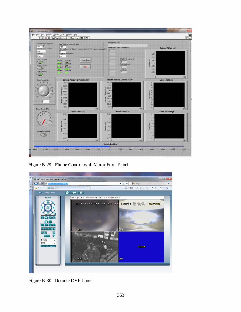
363

Figure B-29. Flume Control with Motor Front Panel

Figure B-30. Remote DVR Panel

364

Figure B-31. Windows Remote Desktop Software

365

APPENDIX C SERF COMPUTER CONTROL PROGRAMS

C.1 Introduction

Because of the enhancements, improvements, and additions to the SERF, most computer

control programs for the device had to be rewritten. Some components from the original

programs were still usable, but the overall structure of the programs changed. Before discussing

in detail, some background should be given. Programs are written in Labview; before modifying

any of these programs, future operators should learn Labview. If changes or modifications are to

be made to any of the programs, the programs should first be backed up so that the current

working programs are not overwritten.

SERF programs have gone through a three generation progression – first with Trammel,

then with Slagle, and finally Crowley’s third-generation programs. The basic purposes of two of

these programs have not changed much over the years. Generally, a motor mover and a primary

control exist. The motor mover has served as a stand-alone program to move the stepper motor

up and down when loading a sample into the device. Secondarily, the motor mover is used as a

sub-vi component in the primary control program. The primary control program is to be used to

run erosion-rate tests.

From Trammel to Slagle, the basic principle of the SERF control programs did not change,

nor did their structure. The algorithm for the control programs was:

1. Read SEATEK signals 2. Read analog (pressure transducer and thermocouple) signals 3. Move the motor 4. Write SEATEK and averaged analog data to a file

In Trammel’s original program, SEATEK data, which takes a second or two to read, was

recorded in the computer memory. Then, analog data, whose timing is based on sampling

frequency and sampling time, was saved into the computer memory. Next, analog data was

366

averaged over the sampling time domain, and an average analog signal was recorded along with

a massaged SEATEK signal (Slagle and Trammel used different methods for this). At the end of

a loop through the program, a user was left with a depth reading, a sample position reading, an

average pressure transducer reading, and an average temperature reading.

The problem with this algorithm is that it is slow and CPU intensive. Allowing the

computer to keep high amounts of analog and digital information in memory, perform

computations on it, etc. caused a loop to take several seconds. When erosion rates were high this

meant that by the time the motor should have moved again, its updated position was already out

of date. The other issue was that at no point in the algorithm was a raw analog signal ever

captured. Rather, it was averaged over the sampling time domain. This meant that any spectral

analysis from an analog signal was impossible.

Slagle recognized the issues with the original SERF programming setup, and he tried to

address them. Slagle’s solution was first to try to speed up Trammel’s original programs and to

reduce their errors. Trammel originally eliminated zeros from the SEATEK number string

(which are caused by false depth readings) by using an “eliminate zeros from string” command.

Slagle changed this to an “eliminate zeros from array” command, which is faster. Slagle tried to

improve the SEATEK depth average by programming a rather rudimentary module where

individual crystals from the 8-crystal inner SEATEK array could be turned off. Slagle also

added a module in his program that eliminated the maximum and minimum SEATEK reading

from the depth average so that a more representative average depth was computed.

During longer-duration tests, Slagle realized that erosion rates were slow. This gave Slagle

the opportunity to add a second SEATEK average depth component to his program. Slagle

differentiated between “rock” erosion programs and “normal” erosion programs via this

367

additional SEATEK depth module. During a “rock” test, the SEATEK took a secondary depth

reading before the motor was allowed to move. If secondary SEATEK reading did not

correspond to the first reading, he assumed that one of the readings must have been in error. The

motor was only allowed to move when both back-to-back SEATEK readings indicated that

movement was necessary.

To speed up his programs further, Slagle realized that reading shear stress from a pressure

difference was difficult. His other analog signal – a temperature reading from a thermocouple –

was not a critical component in the overall system. Therefore, Slagle designed two programs

called “slim” programs where analog signal capturing was eliminated. As a result of this, the

SEATEK-motor loop sped up a little bit more and the used a little bit less CPU power. When

Slagle was done his modifications, he was left with five programs – the motor mover, a rock

program, a slim rock program, a normal program, and a slim normal program.

Slagle’s programs were a welcome improvement to SERF control, but parts of them were

still rather elementary, and although some timing elements were incorporated in them, there was

more work that could be done. With the addition of the lasers and the computerization of the

pump – analog components that could not be ignored using a slim design – the opportunity was

perfect for a program overhaul.

Because of the addition of the lasers, in the new computer programs, Slagle’s dual-layer

SEATEK control was eliminated. The lasers are a precise enough check for SEATEK data

without the dual-layered system. This eliminated the need for Slagle’s rock programs. To allow

for “slimmish” designs, buttons and case structures were added to the overall normal program so

that different components could be turned on or off. Slagle’s “slim” concept was reversed such

368

that a program was written to capture only analog signals; this program is to be used for shear

stress tests. Another program was written to execute pump control.

Currently, there are four updated computer programs that can be used to control the SERF:

• Pump Control • Motor Mover • SERF Control No Motor • SERF Control Full

Programs are found in the G:\SERF_control_new directory on the SERF computer.

Generally, programs begin with the three-letter extension “raf” because they were written by Raf

Crowley and starting programs with the same three-letter extension was an easy way to

differentiate them from other programs. A program in Labview is also generally called a “vi”

(pronounced vee-eye). In this discussion, the terms “program” and “vi” will be used

interchangeably.

C.2 Pump Control

The pump control program is a brand-new SERF control program. Previously, pump

controls were coordinated with the digital display drive in the control room (Figure C-1). A

logical step in SERF development was to computerize the primary SERF pump. Although when

running on two pumps the SERF’s second pump still needs to be run manually, computerizing

the variable speed pump gives more computer control than before. When Trammel set up the

SERF, he hard-wired the pump so that it could be controlled by a computer. Over the years, this

design characteristic was forgotten, and nobody connected the wires to the analog control box.

To connect the pumps to the computer, a set of wires simply needed to be added from the pump

control box to the computer’s SC-2345 analog reader/writer.

One common improvement that was made to the Slagle/Trammel generation of SERF

programs was the incorporation of timing using flat sequence structures. This theme will be

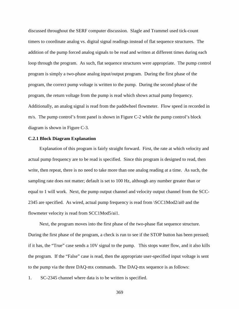
369

discussed throughout the SERF computer discussion. Slagle and Trammel used tick-count

timers to coordinate analog vs. digital signal readings instead of flat sequence structures. The

addition of the pump forced analog signals to be read and written at different times during each

loop through the program. As such, flat sequence structures were appropriate. The pump control

program is simply a two-phase analog input/output program. During the first phase of the

program, the correct pump voltage is written to the pump. During the second phase of the

program, the return voltage from the pump is read which shows actual pump frequency.

Additionally, an analog signal is read from the paddwheel flowmeter. Flow speed in recorded in

m/s. The pump control’s front panel is shown in Figure C-2 while the pump control’s block

diagram is shown in Figure C-3.

C.2.1 Block Diagram Explanation

Explanation of this program is fairly straight forward. First, the rate at which velocity and

actual pump frequency are to be read is specified. Since this program is designed to read, then

write, then repeat, there is no need to take more than one analog reading at a time. As such, the

sampling rate does not matter; default is set to 100 Hz, although any number greater than or

equal to 1 will work. Next, the pump output channel and velocity output channel from the SCC-

2345 are specified. As wired, actual pump frequency is read from \SCC1Mod2/ai0 and the

flowmeter velocity is read from SCC1Mod5/ai1.

Next, the program moves into the first phase of the two-phase flat sequence structure.

During the first phase of the program, a check is run to see if the STOP button has been pressed;

if it has, the “True” case sends a 10V signal to the pump. This stops water flow, and it also kills

the program. If the “False” case is read, then the appropriate user-specified input voltage is sent

to the pump via the three DAQ-mx commands. The DAQ-mx sequence is as follows:

1. SC-2345 channel where data is to be written is specified.

370

2. Voltage is output from SC-2345 to the pump. 3. DAQ-mx task is cleared.

Voltage is calibrated such that the user inputs frequency in the front panel. If someone

wanted to change this, it would be easy to change the calibration to allow for a velocity or

volumetric flow rate instead. SERF operators were moving from a using the manual digital

display control which only has a frequency output. Familiarity with using frequency for the

pump input is why another parameter was not used instead.

During the second phase of the flat sequence structure, the computer is told which channels

on the SC-2345 are to be read. One similarity between the current generation of SERF programs

and the Slagle/Trammel programs is the use of a sub-vi to initiate the DAQ-mx data reading

sequence ([a] in Figure C-3). The block diagram for the pump sub-vi

(raf_DAQ_pump_output.vi) is shown in Figure C-4. The structure of this sub-vi is the same as

Trammel and Slagle’s. The algorithm is as follows:

1. Create the DAQ-mx task 2. Specify the first channel to read. 3. Specify the second channel to read (more channels can be added if necessary). 4. Use a sample clock to input the correct sampling rate.

Output from the sub-vi is sent back to the pump control block diagram. Then, a new

DAQ-mx task is started to read everything from the channels that were specified in the sub-vi.

Finally, the signal is split between so that the velocity signal and the actual pump frequency

signal are isolated from one another. Lastly, the signals are calibrated so that instead of a voltage

output, a velocity or pump frequency output is given.

The wait timer, [b] is a new addition to SERF control programs. Slagle and Trammel did

not realize that this simple addition frees up computer memory. Generally, addition of a wait

timer in a Labview program in between each loop is considered good programming practice.

371

This component should not be removed from any of the new SERF computer programs. Once

the while loop waits the specified number of seconds (10 ms in this case), the loop repeats. The

block diagram’s loop will continue to repeat until the user pushes the large stop button on the

front panel.

C.2.2 Front Panel Operation

To operate the pump control, press the Labview start button on the top of the program.

Then, press “FWD” on the digital pump display to initialize the pump. Failure to press “FWD”

will not allow the pump to run, and this is a common error. Move the slider on the front panel to

the desired pump frequency or alternatively input the pump frequency in the number box. The

pump should start moving water through the flume and real-time frequency and velocity graphs

should be generated. The max flow rate button should not be changed from 1000 gpm unless the

setting on the flowmeter is also changed. The max flow rate in this box corresponds to the data

range coming from the flowmeter (Figure C-5).

C.3 Motor Mover

The motor mover is the one SERF component that has hardly changed over the years. In

2010, Labview components were updated from Labview 7.1 to Labview 2009. Some of the old

motor mover commands have changed since the 7.1 version of Labview, but overall the program

remains the same. The changes result from slightly different syntax requirements between 2009

Labview and Labview 7.1. A screenshot of the Motor Mover’s front panel is shown in Figure C-

6 while a screenshot of its block diagram is shown in Figure C-7.

C.3.1 Block Diagram Discussion

The algorithm for the motor mover is as follows:

1. Specify the movement axis. For the stepper motor, only one axis, Axis 1, moves.

372

2. Specify the Board ID. Board ID corresponds to the slot in which the motion controller (a National Instruments PCI 7330 Card) is plugged in the control computer. With the current SERF setup, the PCI 7330 is plugged into Slot #1.

3. Specify the velocity, acceleration, deceleration, and jerk quantities. None of these should be changed.

4. Read the current motor position. The default is for the motor to start at 0 when the Motor Mover program is first run. If the user wants to reset its overall position, press the reset switch on the front panel and press start.

5. Read relative vs. absolute position. The current setting as shown is relative position. This should not be changed.

6. Set the target position.

7. Initiate movement.

8. Continually move the motor and monitor movement for errors.

9. Stop movement when target position is reached.

C.3.2 Front Panel Discussion

First, input the target position in steps. One centimeter equals 7874 steps. Then, press

start. The motor should move. Press the reset switch and press start to move the computer

position back to zero. The End Position Indicator should return the motor’s position every time

the program is run. The program will stop automatically when the final position is reached.

C.4 SERF Control No Motor

As discussed in Appendix B, shear stress tests should be run independently from erosion

rate tests until a velocity profiler can be installed in the SERF. The Full Version of the control

program can be used to conduct a shear stress test by turning off several of the buttons, but

another stand-alone program was written as well to be used for shear stress tests. The stand-

along program is the same as the first few steps of the full version of the control program, but

there is much less clutter on its front panel – thereby making it a little bit easier to operate. A

373

screenshot of the front panel for SERF Control No Motor is shown in Figure C-8 while a

screenshot of its block diagram is presented in Figure C-9.

C.4.1 Block Diagram Discussion

The block diagram for SERF Control No Motor is similar to the pump control program.

Both vi’s are a two-phase flat sequence structure.

C.4.1.1 SC-2345 channels

First, SC-2345 channels are specified. Figure C-10 zooms in on this portion of the

algorithm. Following Figure C-10 is a list of the way everything is currently wired in the SC-

2345.

• thermocouple (temperature channel): SCC1Mod1/ai0 • flowmeter: SCC1Mod5/ai1 • pressure transducer: SCC1Mod5/ai0 • actual pump frequency (pump box): SCC1Mod2/ai0

To explain the shear stress sensor’s wiring, the sub-vi in Figure C-10 needs to be

explained. A screenshot of this sub-vi is shown in Figure C-11. On the front panel for the SERF

Control No Motor Program, one of the inputs is for the shear stress sensor’s range. Recall from

Chapter 4 that range can be adjusted on the shear stress sensor’s amplifier so that more accurate

readings can be obtained at lower shear stresses. Like the flowmeter with the pump control

program, the range from the instrument must equal the range in the Labview program. Four

wires come from the shear stress sensor; each wire corresponds to a different output range. The

sub-vi shown in Figure C-11 takes the user input range and compares it with the possibilities

from the from the shear stress sensor – 10 Pa, 20 Pa, 50 Pa, and 100 Pa. Then, an array is built

with three zero values. The last value in this array corresponds to an actual channel in the SC-

2345 based on the results from the four case structures shown in the figure. The array max/min

374

command returns the maximum value from this array so that the computer knows which channel

is the correct channel from which to read during shear stress tests.

In addition to specifying which SC modules are to be read, the vi also asks where the user

wants to save data. In general programs were written so that .dat files were generated. This

makes Matlab analysis the easiest. The .dat extension can be changed to .xls for an Excel file or

.txt for a text file.

C.4.1.2 Pump input

The next step in this program uses the first part of the pump control program as a sub-vi.

The user specifies a pump frequency, the pump program is run, and the pump begins. A

screenshot of this sub-vi is shown in Figure C-12.

C.4.1.3 Analog output

The last step in the SERF Control No Motor is also the same as it is with the pump control

program except that five analog signals are taken instead of two. The only thing that changes

between these two programs is that the analog reader in the second half of the case structure now

has five channels. In the base program, the analog signal is now split five times instead of two

(Figure C-13 and Figure C-14).

The case structure surrounding the analog-read portion of the base vi is to allow for manual

data acquisition. During a shear stress test, a SERF operator specifies a flow rate, waits for flow

to stabilize, and collects data. Then, he or she presses “Run” in the base vi and data is collected.

The “true” case for the case structure corresponds to when the “Run” button is pressed while the

“false” case corresponds to when no button is pressed.

As the base vi runs, real-time graphs are generated because of this true-false sequence.

During “false” execution, analog signals are sampled one time through the loop, and the results

are plotted immediately. During “true” execution, raw data is sampled at the specified sampling

375

rate according to the Samples Per Channel input parameter. Then, this data sequence is written

to the appropriate .dat file. This portion of the program is much different than Slagle’s or

Trammel’s. Slagle and Trammel both captured an analog block of data every time through the

Labview loop, averaged it, and wrote the average to the output file. The acquisition of raw data

allows for more advanced data analysis.

C.4.2 Front Panel Operation

To operate raf_data_control.vi:

1. Specify the shear stress range using the drop down menu.

2. Specify the maximum flow rate being used in the flowmeter.

3. Specify the number of samples per analog channel.

4. Specify the sampling rate in Hz.

5. Press the Labview “Run” button

6. Initialize the Pump by pressing “FWD”

7. Bring the pump to the desired flow speed using either the computerized pump dial or the number input below the pump dial.

8. When flow speed and shear stress have leveled out, press “Run” to record a burst of raw data. Data time can be computed by t = N/f where N is the number of samples per channel and f is the sampling frequency.

9. When data is taken, the real-time graphs on the front panel will freeze. When data is done being taken, the graphs will resume moving. If this happens, it means the program is working as designed.

C.5 SERF Control Full (Temperature Patch)

The latest edition of the full version of the SERF control program incorporates a feedback

loop between the thermocouple and the SEATEK, or a temperature patch (hence the program’s

name). The full version of the program is the most complicated program written for the device

and it uses portions of the other programs. Figure C-15 shows a screenshot of front panel for the

376

full version of the SERF control computer program. Figure C-16 shows a screenshot of the

program’s block diagram.

C.5.1 SERF Control Full Block Diagram Discussion

Like the other SERF control programs, the full control program is a multi-phased flat

sequence structure. The following is a discussion of its components.

C.5.1.1 Pre-input sequence

As with other analog SERF programs, the first step in the full version of the control

program is to specify input channels for analog devices. This step is the same as it was for the

control program without the motor except that the lasers’ input channels also must be specified.

As wired right now, the lasers are run through SCC1Mod6/ai0 and SCC1Mod6/ai1 (Figure C-

17). Although there are three lasers installed in the device, they are hard-wired in an “or” logic

sequence. This will be discussed in Section C.5.1.6, but for now, it is sufficient to say that there

are only two sets of wires coming from the laser system. The unique pre-input element to the

full version of the control program is a serial port read-write sequence (Figure C-18).

The sub-vi in Figure C-18 was taken verbatim from the NI examples folder and should not

be changed. The sub-vi sends a “N 1; Enter” command to the SEATEK, waits for 200 ms, and

then reveals an optional output that shows that the number of samples to be taken per SEATEK

burst is indeed one. Previous SERF testing procedures called for a user to open a HyperTerminal

session, specify the number of samples to be taken during a test, and start a data run. When a

SEATEK data run is started, the SEATEK pings each of its crystals at 5 MHz, takes an average

over 1 s, and then outputs its result. The SEATEK “N” command corresponds to the number of

times this pinging-averaging is to repeat itself. Once a SEATEK data run is started, output data

will continue to be generated until the number of bursts from the SEATEK equals N. When a

data run is started, new input parameters cannot be added to the SEATEK until N is met. For the

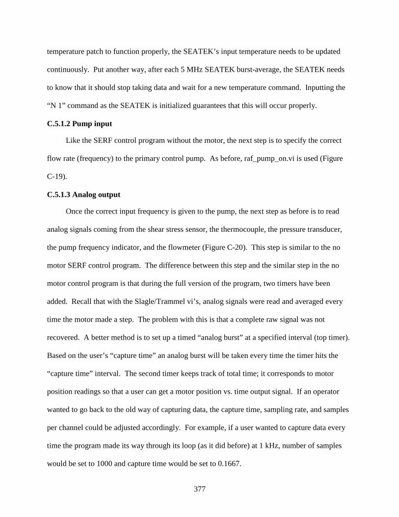
377

temperature patch to function properly, the SEATEK’s input temperature needs to be updated

continuously. Put another way, after each 5 MHz SEATEK burst-average, the SEATEK needs

to know that it should stop taking data and wait for a new temperature command. Inputting the

“N 1” command as the SEATEK is initialized guarantees that this will occur properly.

C.5.1.2 Pump input

Like the SERF control program without the motor, the next step is to specify the correct

flow rate (frequency) to the primary control pump. As before, raf_pump_on.vi is used (Figure

C-19).

C.5.1.3 Analog output

Once the correct input frequency is given to the pump, the next step as before is to read

analog signals coming from the shear stress sensor, the thermocouple, the pressure transducer,

the pump frequency indicator, and the flowmeter (Figure C-20). This step is similar to the no

motor SERF control program. The difference between this step and the similar step in the no

motor control program is that during the full version of the program, two timers have been

added. Recall that with the Slagle/Trammel vi’s, analog signals were read and averaged every

time the motor made a step. The problem with this is that a complete raw signal was not

recovered. A better method is to set up a timed “analog burst” at a specified interval (top timer).

Based on the user’s “capture time” an analog burst will be taken every time the timer hits the

“capture time” interval. The second timer keeps track of total time; it corresponds to motor

position readings so that a user can get a motor position vs. time output signal. If an operator

wanted to go back to the old way of capturing data, the capture time, sampling rate, and samples

per channel could be adjusted accordingly. For example, if a user wanted to capture data every

time the program made its way through its loop (as it did before) at 1 kHz, number of samples

would be set to 1000 and capture time would be set to 0.1667.

378

The “Manual Analog Override” button functions the same way as the “Run” button in the

version of this program without the motor. If the user turns off the motor, the lasers, and the

SEATEK buttons on the front panel, the full version of the program will skip the last three

phases of the five-phase flat sequence structure, and the program will effectively run the same as

the version of the program without the motor. The sub-vi shown in Figure C-20 is similar

enough to the SERF Control No Motor code that it does not need to be shown here.

C.5.1.4 Laser input

The third phase of the five-phase flat sequence structure is to read the voltage signal from

the lasers (Figure C-21). Although the laser output signal is also just another analog signal, there

should not be a need to capture or sustain an analog burst. Output from the lasers is simply a

+10 V reading if the lasers’ photoelectric sensor picks up a light signal or a 0 V reading if the

sensors do not pick up a light signal. Because there was no need to pick up a raw laser signal,

this element from the program was conducted separately. This phase was also programmed

separately so that the lasers could be turned off easily using the front panel. The sub-vi in this

phase of the program is shown in Figure C-22. It should be obvious from its structure that this

sub-vi functions like the second phase of the pump control program. Data from lasers is picked

up, split, and output to the base program.

C.5.1.5 SEATEK output

Once data from the lasers is read, data must next be taken from the SEATEK (Figure C-

23). Unique to this SEATEK output module compared with previous versions of the control

program is a series of buttons for each of the eight inner SEATEK crystals. In his thesis, Slagle

set up the groundwork for a system where individual crystals could be turned off, but using his

program was not intuitive and required block-diagram input. The buttons shown in Figure C-23

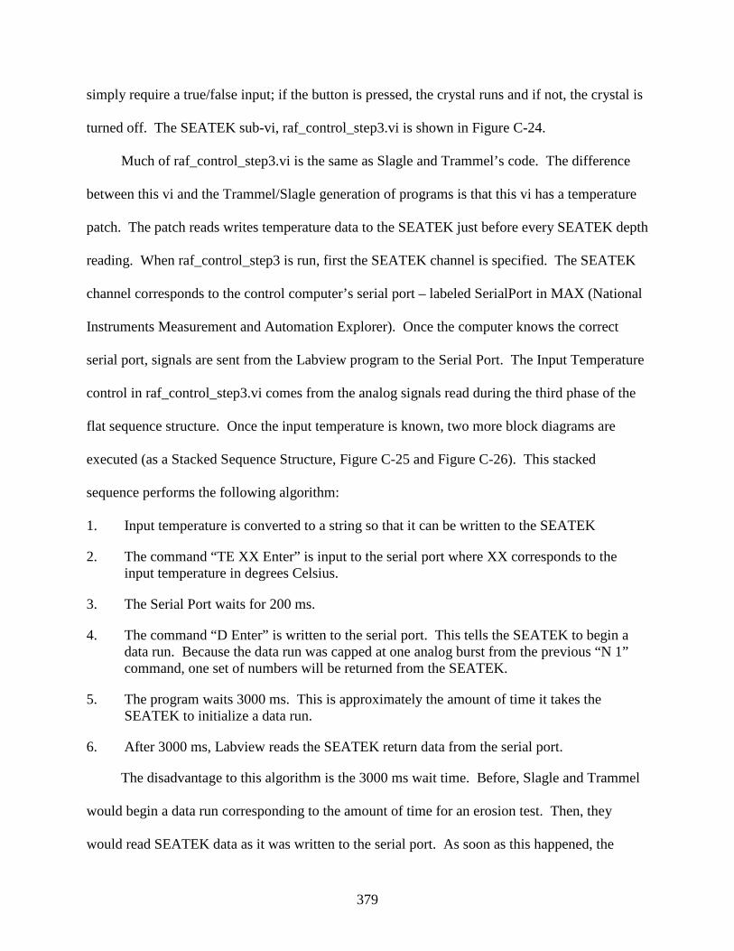
379

simply require a true/false input; if the button is pressed, the crystal runs and if not, the crystal is

turned off. The SEATEK sub-vi, raf_control_step3.vi is shown in Figure C-24.

Much of raf_control_step3.vi is the same as Slagle and Trammel’s code. The difference

between this vi and the Trammel/Slagle generation of programs is that this vi has a temperature

patch. The patch reads writes temperature data to the SEATEK just before every SEATEK depth

reading. When raf_control_step3 is run, first the SEATEK channel is specified. The SEATEK

channel corresponds to the control computer’s serial port – labeled SerialPort in MAX (National

Instruments Measurement and Automation Explorer). Once the computer knows the correct

serial port, signals are sent from the Labview program to the Serial Port. The Input Temperature

control in raf_control_step3.vi comes from the analog signals read during the third phase of the

flat sequence structure. Once the input temperature is known, two more block diagrams are

executed (as a Stacked Sequence Structure, Figure C-25 and Figure C-26). This stacked

sequence performs the following algorithm:

1. Input temperature is converted to a string so that it can be written to the SEATEK

2. The command “TE XX Enter” is input to the serial port where XX corresponds to the input temperature in degrees Celsius.

3. The Serial Port waits for 200 ms.

4. The command “D Enter” is written to the serial port. This tells the SEATEK to begin a data run. Because the data run was capped at one analog burst from the previous “N 1” command, one set of numbers will be returned from the SEATEK.

5. The program waits 3000 ms. This is approximately the amount of time it takes the SEATEK to initialize a data run.

6. After 3000 ms, Labview reads the SEATEK return data from the serial port.

The disadvantage to this algorithm is the 3000 ms wait time. Before, Slagle and Trammel

would begin a data run corresponding to the amount of time for an erosion test. Then, they

would read SEATEK data as it was written to the serial port. As soon as this happened, the

380

depth data was recorded. The temperature patch, because of its 3200 ms wait time (which is

required and should not be changed) sacrifices a certain amount of speed for accuracy.

Some quick mathematics can be used to show why the temperature patch should be

effective. The speed of sound in water is temperature dependent such that a change of one

degree Celsius corresponds to approximately a change in sound speed of approximately 3.1 m/s.

Although the water chiller can hold water temperature steady with approximately 2 degrees

Celsius accuracy, this uncertainty could correspond to as much as 12.4 m/s in speed of sound

uncertainty. As originally conceived, devices like the SEATEK are generally used under field

conditions – where temperatures do not vary drastically and where +/- a few centimeters of depth

accuracy is acceptable. Because of the SERF’s sensitivity requirements for motor advancement

(0.5 mm), a few centimeters of depth accuracy is unacceptable. Slagle realized this; hence his

inclusion of the user-defined depth parameter in his generation of programs. Although

quantitatively tests were not conducted to determine average SEATEK error with and without

the temperature patch, qualitatively, it was clear that as soon as the temperature patch was

designed the user-defined depth parameter was no longer necessary. Therefore, the SEATEK

program went back to using the four outside crystals to define the fixed distance from the top to

bottom of the flume (Figure C-27 or the bottom portion of the full block diagram).

One of the outside crystals was damaged when this project began and was not working.

The malfunctioning crystal consistently returns a low reading. For example, if bottom depth

should be 4.92 cm, actual depth reading from the malfunctioning crystal holds steady at

approximately 3.30 cm. To combat this problem, this crystal is automatically eliminated by

eliminating the minimum value from the array of readings from the SEATEK. If somehow the

entire SEATEK reading gets botched, a case structure is included with a user-defined bottom

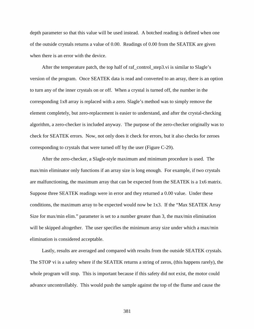
381

depth parameter so that this value will be used instead. A botched reading is defined when one

of the outside crystals returns a value of 0.00. Readings of 0.00 from the SEATEK are given

when there is an error with the device.

After the temperature patch, the top half of raf_control_step3.vi is similar to Slagle’s

version of the program. Once SEATEK data is read and converted to an array, there is an option

to turn any of the inner crystals on or off. When a crystal is turned off, the number in the

corresponding 1x8 array is replaced with a zero. Slagle’s method was to simply remove the

element completely, but zero-replacement is easier to understand, and after the crystal-checking

algorithm, a zero-checker is included anyway. The purpose of the zero-checker originally was to

check for SEATEK errors. Now, not only does it check for errors, but it also checks for zeroes

corresponding to crystals that were turned off by the user (Figure C-29).

After the zero-checker, a Slagle-style maximum and minimum procedure is used. The

max/min eliminator only functions if an array size is long enough. For example, if two crystals

are malfunctioning, the maximum array that can be expected from the SEATEK is a 1x6 matrix.

Suppose three SEATEK readings were in error and they returned a 0.00 value. Under these

conditions, the maximum array to be expected would now be 1x3. If the “Max SEATEK Array

Size for max/min elim.” parameter is set to a number greater than 3, the max/min elimination

will be skipped altogether. The user specifies the minimum array size under which a max/min

elimination is considered acceptable.

Lastly, results are averaged and compared with results from the outside SEATEK crystals.

The STOP vi is a safety where if the SEATEK returns a string of zeros, (this happens rarely), the

whole program will stop. This is important because if this safety did not exist, the motor could

advance uncontrollably. This would push the sample against the top of the flume and cause the

382

sample to rub against the SEATEK crystals. This would scratch the SEATEK’s crystals. This

mechanism is probably why so many of the SEATEK crystals currently do not work. The

raf_control_step3.vi sub-vi returns a bottom offset, outside crystal depth, a raw SEATEK string,

and SEATEK data after data manipulation to the base program.

C.5.1.6 Motor advancement

The motor advancement phase is the last portion of the SERF control program (Figure C-

30). In the base portion of the program, SEATEK depth and laser output are fed into a sub-vi

called raf_control_step4.vi (Figure C-31). The output from this sub-vi is sample position in

steps. There are three case structures programmed in this sequence shown in Figure C.5.17:

1. The far left case structure corresponds to when the flume is run with the lasers only.

2. The middle case structure corresponds to when the flume is run with the SEATEK only.

3. The far right case structure corresponds to when the flume is run with the SEATEK and lasers in a redundant system.

In the case where the lasers are used exclusively, the lasers return a positive voltage only if

their corresponding photoelectric sensor picks up light. When the photoelectric sensor picks up

light, a voltage of ~+16 V is returned; in the program a comparison voltage of + 10 V is used,

although this number is arbitrary. Recall that two lasers are wired to one control box such that

they respond via “or” logic – i.e. a voltage will be returned if either of their photoelectric sensors

picks up light. Experience with the SERF has shown that generally samples erode back-to-front

or front-to-back. It is rare to see a sample stay intact in its center while exhibiting high erosion

rates in the back and the front. This why the outside lasers were chosen for the “or” logic, while

the middle laser was wired by itself. When either of these outside lasers plus the middle laser are

uncovered, the sample advances. Although it would have been better to wire lasers

383

independently with one another, this would have been more expensive, and funding was not

available for it. This solution was the most effective alternative.

In the case where the SEATEK is used by itself, depth data from the base program is

written to raf_control_step4.vi. If the bottom offset distance is greater than 0.5 mm, the sample

advances. If the bottom offset distance is less than -0.5 mm, the sample retracts. The retraction

allows for a constant depth-check. If the sample has advanced too much (which happens

sometimes), the retraction allows for a correction to be made.

In the case where the SEATEK and the lasers are used together, the retraction algorithm

does not change from the case where the SEATEK is used by itself. The weakness of the lasers

is that they do not provide any retraction information should the sample advance too far into the

flume. In the advancement case, an “and logic” sequence is programmed where laser output plus

SEATEK output are both needed to trigger movement. In every case, the sub-vi that controls

movement is the same raf_motor_mover.vi describe in Section C.5.3.

C.5.1.7 Data writing

Data writing is somewhat different in this program than it was in the Slagle and Trammel

versions. Previously, data was written to one data file. Now, because analog bursts are taken to

recover the original analog signal, two output files need to be generated – one for analog data

and the other for piston position data. The analog burst data is written during the analog phase of

the flat sequence structure while the depth data is written after the motor advances.

C.5.2 Using the Front Panel

The front panel improvements to the full version of the SERF control program are

significant because for the first time ever, a user has touch-of-the-finger control on any of the

device’s components. The front panel is much more user-friendly than it was in the past.

384

Although using the front panel should be self-explanatory, the following is an example of how to

use it:

1. Specify shear stress range (if shear stress readings are to be taken), sampling frequency, number of samples per channel, capture time, and the minimum SEATEK size to be used for max/min elimination.

2. Turn off any malfunctioning SEATEK crystals (if the SEATEK is to be used).

3. Decide what kind of data run is to be used. Options include:

a. Analog capture only using Manual Analog Override

b. Erosion test

c. With Lasers only

d. With SEATEK only

e. With both lasers are SEATEK

4. Specify flow rate.

5. Press “FWD” on the pump’s digital control.

6. Press the “RUN” button.

7. The program will ask where to save the two .dat files. Specify the directory.

8. The SERF should run until the “STOP” button is pressed.

385

Figure C-1. SERF Digital Control Display

Figure C-2. Pump Control Program Front Panel

386

Figure C-3. Block Diagram for Pump Control Program (raf_pump_control.vi)

[a] [b]

387

Figure C-4. Analog Reader Sub-vi (raf_DAQ_pump_output.vi)

Figure C-5. View from Top of Flowmeter Showing Data Range. See flowmeter’s operating manual for directions on how to change it settings.

388

Figure C-6. Motor Mover Front Panel

Figure C-7. Motor Mover Block Diagram (raf_motor_mover.vi)

389

Figure C-8. SERF Control No Motor Front Panel

390

Figure C-9. Block Diagram for SERF Control No Motor (raf_data_control.vi)

391

Figure C-10. Zoom-in on SC-2345 Channels.

Figure C-11. Shear Stress Calibration Sub-vi (raf_shear_module.vi)

392

Figure C-12. Sub-vi Showing First Portion of Pump Control Program (raf_pump_on.vi)

Figure C-13. Analog Reader for SERF Control No Motor (raf_DAQ_no_motor.vi)

393

Figure C-14. Five Signal Split in Pump Control No Motor

394

Figure C-15. Front Panel for SERF Control With Motor and Temp Patch (raf_control5.vi)

395

Figure C-16. Block Diagram for SERF Control With Motor (raf_control5.vi

396

Figure C-17. Analog Input Channels for raf_control5.vi

Figure C-18. Initial Read-Write Sequence Between for SEATEK Serial Port (SEATEK_integrate.vi)

397

Figure C-19. First Phase of Five-Phase Flat Sequence Structure Showing the Pump Input Controller (raf_pump_on.vi)

Figure C-20. Second Phase of Five-Phase Flat Sequence Structure Showing the Analog Output Module. Sub-vi is called raf_control_step1-1.vi.

398

Figure C-21. Third Phase of Five-Phase Flat Sequence Structure Showing the Laser Output Module (raf_control_step2.vi)

Figure C-22. Block Diagram for raf_control_step2.vi

399

Figure C-23. Fourth Phase of Five-Phase Flat Sequence Structure Showing the SEATEK Output Module. Sub-vi is called raf_control_step3.vi.

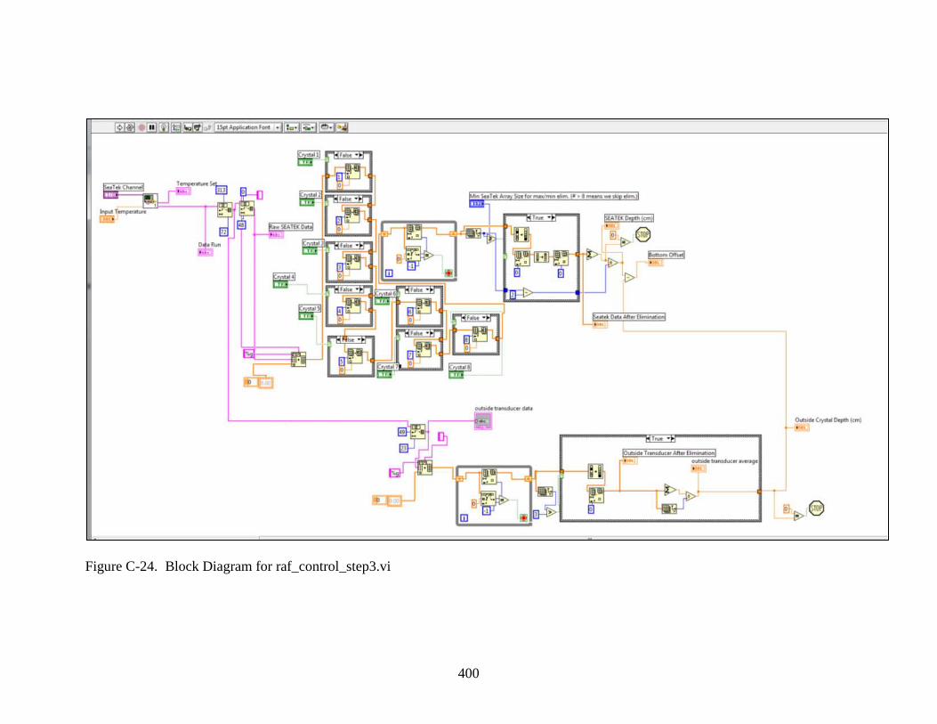
400


401

Figure C-25. First Element in Temperature Patch Stacked Sequence Structure

Figure C-26. Second Element in Temperature Patch Stacked Sequence Structure

402

Figure C-27. Outside Crystal Depth Algorithm

Figure C-28. Example of a Crystal-Off Module with Crystal 2 Shown

Figure C-29. SEATEK zero-checker. Algorithm is the same as Slagle’s.

403

Figure C-30. Fifth Phase of Five-Phase Flat Sequence Structure Showing the Motor Movement Module

404


405

LIST OF REFERENCES

Annandale, G. W., Smith, S.P., Nairn, R. and Jones, J.S. (1996). “Scour power.” Journal of Civil Engineering, July, 58-60, cited in Slagle, P.M. (2006). Annandale, G.W. (2005). Scour technology. McGraw-Hill, New York. Ariathurai, R. (1974). “A finite element model for sediment transport in estuaries.” Ph.D. dissertation, University of California, Davis, CA. Bagnold, R. A. (1956). “An approach to the sediment transport problem from general physical.” Professional Paper, No. 442-1, USGS, Washington, D.C. Barry, K. M. (2003). “The effect of clay particles in pore water on the critical shear stress of sand.” Ph.D. dissertation, University of Florida, Gainesville, Florida. Barry, K. M., Thieke, R. J., and Mehta, A. J.(2005). “Quasi-hydrodynamic lubrication effect of clay particles on sand grain erosion.” Estuarine and Coastal Shelf Science 67, 161 – 169. Bloomquist, D (2010). Personal conversations and correspondence. Associate Professor, University of Florida, Gainesville, FL. Bollaert, E. and Schleiss, A. (2003). “Scour of rock due to the impact of plunging high velocity jets part I: a state-of-the-art review.” Journal of Hydraulics Research, 00(0), 1 – 14. Bollaert, E. and Schleiss, A. (2003). “Scour of rock due to the impact of plunging high velocity jets part II: experimental results of dynamic pressures at pool bottoms in one- and two- dimensional closed end rock joints.” Journal of Hydraulics Research, 00(0), 1 – 16. Briaud J. L. (2004). “Scour#1 killer of bridges.” Geostrata, The Geotechnical Institute of the American Society of Civil Engineers, Fall. Briaud, J. L., Chen, H. C., Li, Y. and Nurtjahyo, P. (2004a). “The SRICOS-EFA method for complex piers in fine-grained soils.” Journal of Geotechnical and Geoenvironmental Engineering, 130(11), 1180 – 1191. Briaud, J.L., Chen, H. C., Li, Y., Nurtjahyo, P., and Wang, J. (2004b). “Pier and contraction scour in cohesive soils.” NCHRP Report 516, Transportation Research Board, Washington, D.C. Briaud, J. L., Chen, H. C. and Ting, F. (2010). “The, EFA, erosion function apparatus: an overview.” http://tti.tamu.edu/conferences/scour/sample_paper.pdf, March 23, 2010. Briaud, J. L., Ting, F. C. K., Chen, H. C., Gudavalli, R., Perugu, S., and Wei, G. (1999). “SRICOS: Prediction of scour rate in cohesive soils at bridge piers.” Journal of Geotechnical and Geoenvironmental Engineering, 125(4), 237 – 246.

406

Christensen, B. A. (1972). “Incipient motion on cohesionless channel banks.” Symposium to Honor Professor H. A. Einstein, edited by H. W. Shen, Colorado State University, Fort Collins, CO, 1 – 22. Christensen, B. A. (1975). “On the stochastic nature of scour initiation.” Proceedings of the 16th

International Association for Hydraulic Research Congress, Sao Paulo, Brazil (2), 65 – 72. Cokljat, D., Carter, J. G. and Emerson, D. R. (1996). “Calculation of flow in transition duct using second- order closure and wall functions.” American Instittue of Aeronautics and Astronautics, 34(11), 2437 – 39. Cornett, A., Sigouin, N., and Davies, M. (1994). “Erosive response of Northumberland straight till and sedimentary rock to fluid flow.” National Research Council of Canada, Institute for Marine Dynamics, TR-1994-22, September, Ottowa, Canada, 1 – 15, 26 – 27. Crowley, R.W. (2008). “Drag forces on pile groups.” M.S. Thesis, University of Florida, Gainesville, FL. Dade, W. B. and Nowell, A. R. M. (1991). “Moving muds in the marine environment.” Proceedings of the 1991 Conference on Coastal Sediments, ASCE, New York, NY, 54 – 71. Dade, W. B., Nowell, A. R. M., and Jumars, P. A. (1992). “Predicting erosion resistance of muds.” Marine Geology, 105, 285 – 97. Dyer, K. R. (1986). Coastal and estuarine sediment dynamics. Wiley Interscience, Chichester, United Kingdom. Einstein, H. A. (1943). “Flow on a movable bed.” Proceedings from the Second Hydraulics Conference, Iowa City, 27, 332 – 46. Einstein, H.A. (1950). “The bed-load function for sediment transportation in open channel flows.” US Department of Agricultural Technologies, 1026, Washington. Englund F. and Hansen, E. (1972). A monograph on sediment transport in alluvial streams. Technial Press, Copenhagen, Denmark. “Florida department of transportation bridge scour manual (2005).” <http://www.dot.state.fl.us/ rddesign/dr/Bridgescour/FDOT-Scour-Manual-6-2-2005-Final.pdf>, Sept. 2, 2008. Fukada, M. and Lick, W. J. (1980). “The entrainment of cohesive sediments in fresh water.” Journal of Geophysical Research, 85(C5) 2813 – 2824, cited in McNeil, J. (1996). Gessner, F. B., and Emery, A. F. (1980). “The numerical prediction of developing turbulent flow in rectangular ducts.” Journal of Fluids Engineering, 103, 445 – 455.

407

Gordon, S. (1991). “Scourability of rock formations.” Federal Highway Administration Memorandum, July 19, Washington, D.C. Hanson, G. J. and Simon, A. (2002). “Discussion of erosion function apparatus for scour rate predictions by J.L. Briaud, F. C. Ting, H. C. Chen, Y. Cao, S. W. Han, and K. W. Kwak.” Journal of Geotechnical and Geoenvironmental Engineering, 627 – 628. Henderson, M. R. (1999). “A laboratory method to evaluate the rates of water erosion of natural rock materials.” M.S. Thesis, University of Florida, Gainesville FL. Hofland, B. and Battjes, J. A. (2006). “Probability density function of instantaneous drag forces and shear stresses on a bed.” Journal of Hydraulic Engineering, 132, (11), 1169 – 1175. Hjorth, P (1975). “Studies on nature of local scour.” Bulletin Series A, No. 46, Department of Water Resources Engineering, Lund Institute of Technology, University of Lund, Sweden. Jepsen, R., Roberts, J. and Lick, W. (1997). “Effects of bulk density on sediment erosion rates.” Water, Air, and Soil Pollution, 99, 21 – 31. Jepsen, R., Roberts, J. D. and Gailini, J. (2004). “Erosion measurements in linear, oscillatory, and combined oscillatory and linear flow regimes.” Journal of Coastal Research, 20(4), 1096 – 1106. Jones, J. S., Alqalam, Kamel, Gratton, Buddy, Summers, Brian (1995). “Effect of the 1994 southeast flooding on the highway system in Georgia.” Handout from presentation at the 1995 American Society of Civil Engineers Water Resources Engineering Conference, San Antonio, TX., cited in Mueller, J., “Field based research on channel scour at bridges,” <http://water.usgs.gov/osw/techniques/workshop/Mueller.html>, March 22, 2010. Judson, S., Kaufman, M. E. and Leet, L. D. (1987). Physical geology. Prentice-Hall, Englewood Cliffs, NJ. Kandiah, A. (1974). “Fundamental aspects of surface erosion of cohesive soils.” Ph.D. dissertation, University of California, Davis, CA. Kerenyi, K. (2010). Personal conversations. Lead researcher, FHWA Hydraulics Laboratory, McLean, VA. Kerr, K. (2001). “A laboratory apparatus and methodology for testing water erosion in rock materials.” M.E. thesis, University of Florida, Gainesville, Florida. Laufer, J. (1954). “The structure of turbulence in fully developed pipe flow.” Report no. 1174, National Advisory Committee for Aeronautics, Washington, D.C.

408

Lemke, K. A. (2010). “Stream sediment.” University of Wisconsin-Stevens Point, http://www. uwsp.edu/geo/faculty/lemke/geomorphology/lecture_outlines/03_stream_sediment.html, Sept. 14, 2010. MacIntyre, S., Lick, W. and Tsai, C. H. (1990). “Variability of entrainment of cohesive sediments in freshwater.” Biogeochemistry,9, 187 – 209, cited in McNeil, J. (1996). Mantz, P. A. (1977). “Incipient transport of fine grains and flakes by fluids.” Journal of Hydraulics Division of ASCE, 103(6), 601 – 615. McGuire, Mark. “Drafts of Capital region’s severe weather history.” Legacy of Change,

http://web.timesunion.com/specialreports/tu150/stories/weather.asp, Nov. 11, 2010.

McLean, S.R. (1975). “Theoretical modeling of deep sediment transport.” Marine Geology, 66, 243 – 265. McNeil, J., Taylor, C., and Lick, W. (1996). “Measurements of erosion of undisturbed bottom sediments with depth.” Journal of Hydraulic Engineering, 122(6), 316 – 324. Mehta, A. J. (2007). “An introduction to hydraulics of fine sediment transport.” OCP 6297 class notes draft, University of Florida, Gainesville, Florida. Mehta, A. J. and Lee, S. C. (1994). “Problems in linking the threshold condition for the transport of cohesionless and cohesive sediment grain.” Journal of Coastal Research, 10(1), 170 – 177. Mehta, A. J., Parchure, T. M., Dixit, J. G., and Ariathuri, R. (1982). “Resuspension potential of deposited cohesive beds.” Estuarine comparisons, edited by V.S. Kennedy, Academic Press, New York, N.Y, cited in McNeil, J. (1996). Mehta, A. J. and Parachure, T. M. (2000). “Surface erosion of fine-grained sediment revisited.” Muddy coast dynamics and resource management, edited by: Belmming, B. W., Delfontaine, M. T. and Liebezeit, G., Elsevier, Amsterdam, The Netherlands, 55 – 74. Melling, A. and Whitelaw, J. H. (1976). “Turbulent flow in a rectangular duct.” Journal of Fluid Mechanics, 27(2), 289 – 315. Melville, B. W. and Sutherland, A. J. (1988). “Design method for local scour at bridge piers.” Journal of Hydraulic Engineering, ASCE, 125(1), 59 – 65, cited in Slagle, P.M. (2006). Melville, B. W. “ Scour at bridge sites.” Civil engineering practices, vol. 2, edited by Cheremisinoff, N. P., Technomic Publishing, Lancaster, PA, cited in Slagle, P. M. (2006). Meyer-Peter E. and Mueller, R. “Formulations for bed-load transport.” Proceedings for the 2nd Meeting International Hydraulics Research. Stockholm, 39 – 64.

409

Migniot, C. (1989). “Tassement et rheologie des vases, lere partie.” La Houille Blanche, 1, 11 – 29, cited in Mehta, A. J. (2007). Miller, R. L. and Byrne, R. J. (1966). “The angle of repose for a single grain on a fixed rough bed.” Sedimentology, 6, 303 – 314. Miller, William Jr. (2003). “Model for the time rate of local sediment scour at a cylindrical structure.” Ph.D. dissertation, University of Florida, Gainesville, Florida. Mitchener, H. and Torfs, H. (1996). “Erosion of mud/sand mixtures.” Coastal Engineering, 29, 1 – 25. Molinas, A (2003). “Bridge scour in nonuniform sediment mixtures and in cohesive materials: synthesis report.” FHWA Report Number FHWA-RD-03-083, Washington, D.C. Murillo, J.A. (1987). “The scourge of scour.” Civil Engineering, American Society of Civil Engineers, 57(7). Naimi, M. and Gessner, F. B. (1993). “A calculation method for developing turbulent flow in rectangular ducts of arbitrary aspect ratio.” Journal of Fluids Engineering, 117, 249 – 258. Nalluri, C. and Alvarez, E. M. (1992). “The influence of cohesion on sediment behavior.” Water Science and Technology, 25(8), 151 – 164. Neilsen, P. (1992). Coastal bottom boundary layer and sediment transport. World Scientific Publishing, River Edge, NJ. Niraula, L. D. (2004). “Development of modified T-Z curves for large diameter piles/drilled shafts in limestone for FB-Pier.” M.E. Thesis, University of Florida, Gainesville, FL. Obi, K., Inoue, T. S., Furukawa, T., and Masuda, S. (1996). “Experimental study on the statistics of wall shear stress in turbulent channel flows.” International Journal of Heat and Fluid Flow, 17(3), 187 – 192. Papanicolaou, A. N., Diplas, P., Dancey, C. L., and Balakrishnan, M. (2001). “Surface roughness effects in near-bed turbulence: implications to sediment entrainment.” Journal of Engineering Mechanics, 127(3), 211 – 218. Panagiotopoulos, I., Voulgaris, G., and Collins, M. B. (1997). “The influence of clay on the threshold of movement of fine sandy beds.” Coastal Engineering, 32, 19 – 43. Partheniades, E. (1965). “Erosion and deposition of cohesive soils.” Journal of Hydraulics Division of ASCE, 91(1), 105 – 138.

410

Pitocchi, D. (2010). Personal correspondence. Research engineer FDOT State Materials Office, Gainesville, FL. Placzek, G. and Haeni, F. P. (1995). “Surface-geophysical techniques used to detect existing and infilled scour holes near bridge piers.” U.S. Geological Survey Water Resources Investigation Report 95-4009. Raudkivi, A. J. (1990). Loose boundary hydraulics. 3rd Edition, Pergamon Press, Oxford, United Kingdom. Reichardt, H. (1951). “Vollstandige darstellung der turbulenten geschwindig-keitsverteilung in glattern leitungen.” Z. Angew. Math Mech., 31(7) 208 – 19 (in German), cited in Barry, K. (2003). Richardson, E. V. and Davis, S. R. (2001). “Evaluating scour at bridges fourth edition.” Publication No. FHWA NHI 01-001 hydraulic engineering circular no. 18. http://isddc.dot.gov/OLPFiles/FHWA/010590.pdf, Sept. 2, 2008. Roberts, J., Jepsen, R., Gotthard, D., and Lick, W. (2003). “Effects of particle size and bulk density on erosion of quartz particles.” Journal of Hydraulic Engineering, 124, 1261 – 1267. Roberts, S. K., and Yaras, M. I. (2006). “Effects of surface roughness geometry on separation- bubble transition.” Journal of Turbomachinery, (128)349, 349 – 356. Rokni, M., Olsson, C., and Sunden, B. (1998). “Numerical and experimental investigation of turbulent flow in a rectangular duct.” International Journal for Numerical Methods in Fluids, 28, 225 – 242. “Scour Plan of Action (2009).” http://www.dot.ca.gov/hq/structur/strmaint/scour.htm, December 14, 2009. Schlichting, H. (1979). Boundary layer theory, 7th Edition. McGraw-Hill, New York, NY. Sferrazza, L and Williams, M (2002). “Pressurized drums, what every handler should know.” Department of Defense Radioactive Waste Generators Conference, May. Shah, F. D. (2009). “Development and testing of uniform synthetic limestone samples for the calibration of equipment used to determine erosion rates.” Honor’s thesis, University of Florida, Gainesville, FL. Sharif, A.A. (2002). “Critical shear stress and erosion of cohesive soils.” Ph.D. dissertation, State University of New York at Buffalo, New York.

411

Sheppard, D. M. (2010). Personal correspondences and communications. Professor Emeritus, University of Florida, Gainesville, FL. Sheppard, D. M. (2004). “Overlooked local scour mechanism.” Journal of the Transportation Research Board No. 1890, TRB, National Research Council, Washington, D.C., 107 – 111. Sheppard, D. M., Bloomquist, D. and Slagle, P. M. (2006). “Rate of erosion properties of rock and clay (correlation of erosion rate-shear stress relationships with geotechnical properties of rock and cohesive sediments).” FDOT Report for Project Number BD-545, RPWO #3. Sheppard, D. M. and Miller, W. (2006). “Live bed and local pier experiments.” Journal of Hydraulic Engineering, 132(7), 635 – 642. Sheppard, D. M., Odeh, M., and Glasser, T. (2004). “Live-bed local pier scour experiments.” Journal of hydraulic engineering, ASCE, 130(10), 957 – 963, cited in Slagle, P. M. (2006). Shields, A (1936). Application of similarity principles and turbulence research to bed-load movement. Mitteilunger der Preussischen Versuchsanstalt fur Wasserbau und Schiffbau, 26, 5 – 24. Slagle, P. M. (2006). Correlations of erosion rate-shear stress relationships with geotechnical properties of rock and cohesive sediments. M.S. thesis, University of Florida, Gainesville, Florida. Sumer, M. and Fredsoe, J (2006). Hydrodynamics around cylindrical structures. World Scientific Publishing, Hackensack, NJ. Suntoyo, and Tanaka, H. (2009). “Effect of bed roughness on turbulent boundary layer and net sediment transport under asymmetric waves.” Coastal Engineering, (56)9, 960 – 969. Ting, F. C. K., Briaud, J. L., Chen, H. C., Gudavalli, R., Perugu, S., and Wei, G. (2001). “Flume tests for scour in clay at circular piles.” Journal of Hydraulic Engineering, 127(11), 969 – 978. Torfs, H. (1996). “Erosion of mud/sand mixtures.” Ph.D. Thesis, Catholic University of Leuven, Leuven, Belgium. Torfs, H., Jiang, J., and Mehta, A. J. (2000). “An assessment of erodibility of fine/coarse sediment mixtures.” Coastal and estuarine fine sediment transport processes, edited by: McAnally, W. H., and Mehta, A. J., Elsevier, Amserdram, 109 – 123.

412

Trammel, M. A. (2004). “Laboratory apparatus and methodology for evaluating water erosion rates of erodible rock and cohesive sediments.” M.S. thesis, University of Florida, Gainesville, Florida. Tsai, C.H. and Lick, W. (1988). “Resuspension of sediments from Long Island Sound.” Water Science Technology, 20(6/7) 155 – 164, cited in McNeil, J. (1996). Van Prooijen, B. C. and Winterwerp, J. C. (2008). “A stochastic formulation for erosion of cohesive sediments.” Journal of Geophysical Research, Draft Copy, December 9, 2008. Van Rijn, L.C. (1992). Principles of sediment transport in rivers, estuaries, and coastal seas, Aqua Publications, Amsterdam, The Netherlands. Wei, G., Chen, H. C., Ting, F., Briaud, J., Gudavalli, R., and Perugu, S. (1997). “Numerical simulation to study scour rate in cohesive soils.” Report for Texas Department of Transportation, Department of Civil Engineering, Texas A&M University, College Station, TX. Wiberg, P. L. and Smith, J. D. (1987). “Calculations of the critical shear stress for motion of uniform and heterogeneous sediments.” Water Resources Research, 23(8), 1471 – 1480. Yalin, M. S. (1972). Mechanics of sediment transport. Pergamon, New York, NY.

BIOGRAPHICAL SKETCH

Raphael Crowley was born in Syracuse, NY in 1982, and grew up on Skaneateles Lake just

outside of Syracuse. He has always had an interest in engineering and research. In 2004,

Crowley graduated from Bucknell University with a double major in Civil Engineering and

History. While at Bucknell, Crowley began his career in research under the tutelage of Dr.

Richard Crago. Crago and Crowley co-authored two papers for publication during their two

summers of research. In 2004, The Journal of Hydrology published “Complementary

Relationships for Near-Instantaneous Evaporation” and in 2005, Water Resources Research

published “A Complementary Evaporation Approach to the Scalar Roughness Length.”

Although this research was in fluid mechanics and hydrology, Crowley still maintained a strong

interest in structures as well.

After graduation in 2004, Crowley spent a year working in West Nyack, NY, a suburb of

New York City, as a Marine Engineer for M.G. McLaren, P.C. This job allowed Crowley to

combine his interests in fluids with his interests in structures. As Crowley learned more about

the field, he realized that he wanted to return to academia and learn as much as possible about

Marine and Coastal Engineering. In the fall of 2005, Crowley enrolled at the University of

Florida to pursue his post-graduate work.

Upon matriculation at the University of Florida, Crowley began working on his master’s

degree under the tutelage of Dr. D. Max Sheppard. His research was conducted at the Turner

Fairbank Highway Research Center (TFHRC) in McLean, VA under the supervision of Dr.

Kornel Kerenyi. While in VA, Crowley ran small-scale model tests on bridge decks and

cylinders. The goal was to quantify lift and drag forces on the bridge decks, drag forces on the

cylinders, and scour depths under pressure-flow scenarios. Crowley’s Masters Thesis, “Drag

Forces on Pile Groups” was completed in May, 2008.

After completion of his Master Degree, Crowley began working with Dr. David

Bloomquist on erosion rates of rock-like and sand/mud mixtures. Bloomquist hoped to use the

experience that Crowley had gained as a lab-technician and research assistant at the TFHRC to

revitalize and improve UF’s SERF. Improvements to the SERF were completed in December of

2009, and tests involving sand/mud mixtures were completed in August of 2010. Improvements

to the SERF include a state-of-the-art shear-stress measurement system, a vortex generator, and a

water chilling system to allow for multi-day tests. Experiments and data analysis have helped to

answer how to properly measure erosion rates in erosion rate testing devices. The purpose of

this work is to use these results in with methods for predicting local scour depths that require the

input of a sediment transport function.

Crowley’s future plans include converting this dissertation to a series of publishable

papers. Once that is completed, Crowley looks forward to finding employment as an Assistant

Professor or Post-Doc at a four-year College or University so that he can pursue his life-long

dream of following a career in academia.

Documents

INVESTIGATION OF SEDIMENT EROSION RATES OF ROCK ... - University of Floridaufdcimages.uflib.ufl.edu/UF/E0/04/24/76/00001/crowley_r.pdf · mixtures for predicting scour depth using