Computers and Mathematics with Applications ( ) –

Contents lists available at ScienceDirect

Computers and Mathematics with Applications

journal homepage: www.elsevier.com/locate/camwa

Investigation of two-phase flow in porous media using latticeBoltzmann methodMohammad Taghilou, Mohammad Hassan Rahimian ∗

School of Mechanical Engineering, College of Engineering, University of Tehran, Tehran, Iran

a r t i c l e i n f o

Keywords:Two-phase flowPenetrationPorous mediaLattice Boltzmann

a b s t r a c t

In this paper penetration of a liquid drop in a porous media is investigated by the latticeBoltzmann method (LBM). Two-phase flow has been simulated by the Lee method whichis based on the Chan–Hilliard binary fluid theory. The contact angle between solid, liquidand gas phases has been considered in the simulations. The porousmedium is generated bylocating square obstacles randomly in a domain. The Reynolds number, the Froude number,theWeber number, viscosity and density ratios are numbered as the non-dimensional flowparameters which influence the domain. The porosity, the Darcy number and the pore tosolid length ratio are the non-dimensional characteristics of the porous structures affectingthe penetration of liquid inside the porous media. To ensure the validity of the code, therelease of a square drop in the computational field was tested and the equilibrium contactangle between the droplet and solid surface was modeled according to Lee. Penetrationand the non-absorbed coefficient have been presented to show penetration of the drop.Investigation of numerical results showed that increasing the Reynolds number, the Froudenumber, porosity and density ratio will increase the penetration rate while increasing theWeber number causes scattering of the drop.

© 2013 Elsevier Ltd. All rights reserved.

1. Introduction

Wide ranges of droplet penetration applications in porous substrates have led to myriad experimental and numericalinvestigations [1–3]. Any increase in the quality of inkjet printers depends directly on the droplet radius after impingementon a porous surface and its spreading rate. Environmental applications, such as hazard assessment of the accidental releaseof liquids onto the soil [4], are mainly concerned with the evaporation rate of the liquid droplet, which is a function of thewet spot area on the surface of the porous medium, exposed to the atmosphere, as well as the penetration depth. Most ofthe studies focus on the droplet impact on non-permeable and permeable surfaces based on CFD approaches [5–9]. Recentlyresearchers have been trying to develop fluid flowmodeling especially two-phase flows, using the lattice Boltzmannmethod(LBM) because of its exclusive features such as parallelism of computation, capture of the complex geometries and simplecoding. In order to simulate two-phase flows, Shan and Chen [10] proposed a facile method which is executable in complexgeometries. He et al. [11] developed the LBM two-phase modeling by introducing two distinct distribution functions for theevaluation of mass, momentum and pressure, but they did not distinguish between thermodynamic and dynamic pressures.In their work parasitic velocities at the interface area have been reduced, but they did not disappear completely. To simulatethe contact angle in this method, Shiladitya Mukherjee and John Abraham [12] introduced an external force which acts ona wall and its strength controls the wettability of the surface. Recently Lee [13] suggested a two-distribution function LBEmethod in which the incompressibility is enforced by the pressure evolution equation. As long as the intermolecular force is

∗ Corresponding author.E-mail address: rahimyan@ut.ac.ir (M.H. Rahimian).

0898-1221/$ – see front matter© 2013 Elsevier Ltd. All rights reserved.http://dx.doi.org/10.1016/j.camwa.2013.08.005

2 M. Taghilou, M.H. Rahimian / Computers and Mathematics with Applications ( ) –

expressed in the potential form, the incompressible LBE method for binary fluids is able to eliminate parasitic currents. Hismethod can simulate two-phase flow in the wide ranges of density and viscosity ratios (up to 1000). To model the contactline dynamics on partially wetting surfaces T. Lee and L. Liu [14] developed Lee’s method for incompressible binary fluids.

In the current work we have imposed Lee’s method in a porous substrate and investigated droplet dynamics afterimpingement on the permeable surface. Then the effects of flow and substrate characteristics variations have been discussedcomprehensively.

2. Simulation of two-phase flow

2.1. Two-phase flow models

Discretization of the force terms in the LBM is considered as amajor factor causing the numerical instability and limitationin its use in practical cases as the Shan and Chen model. Using a method that uses the proper expression for the pressureterm can be useful in stabilizing the simulations. Taehun Lee in 2005 [15] presented a stable LBM method to simulatethe two-phase flow with high viscosity and density ratios by a low Mach number assumption and utilizing the stressand potential forms of the surface tension force. In the absence of external forces, errors resulting from the discretizationappear as parasitic velocities near the interface area. Numerical instabilitywill increasewith increase in both surface tensionand amount of parasitic velocities. Two mechanisms have been proposed to reduce parasitic velocities in the LBM. One ismodification of the pressure gradients and surface tension terms formulations and the other one is using the sharp interfacemethod [13]. Wagner [16] showed that using the potential form of surface tension instead of the pressure form couldeliminate the parasitic velocities. Lee in 2009 [13] presented a method for simulating the binary fluid flow based on theCahn–Hilliard diffuse interface theory.

2.2. Cahn–Hilliard model

By assuming a binary flow, using the continuity equation for each phase leads to evaluation of composition C as follows:

∂ρi

∂t+ ∇(ρiui) = 0, (1)

where ρi is related to local density and ui is the velocity of the i-th component (i = 1, 2). The total density ρ =2

i=1 ρiis also conserved. For convenience, one chooses the heavier fluid as species 1 and the lighter fluid as species 2. Volumediffusive flow rate ji is related to local density and velocity of the i-th component by

ρiji = ρi(ui − u), (2)where u is the volume averaged velocity, and ρi is the constant bulk density.

By definition of C = ρ1/ρ1, Eq. (1) can be rewritten as∂C∂t

+ ∇(uC) = −∇j1. (3)

If the diffusive flow rate does not relate to the densities but to the local compositions of two components, it yieldsj1 = −j2 = j and from Eq. (3) ∇u = 0. This result is just satisfied in the LBM method at low Mach number. The diffusiveflow rate is related to the gradient of the chemical potential µ by the Cahn–Hilliard advection equation:

j = −M∇µ, (4)whereM > 0 is the constant mobility.

Cahn and Hilliard [17] asserted that the mixing energy density for an isothermal system takes the following form

Emix(C, ∇C) = E0(C) +k2

|∇C |2 , (5)

where k is the gradient parameter and E0 denotes bulk energy by

E0(C) ≈ βC2(C − 1)2, (6)where β is a constant. The classical part of the chemical potential is also derived by the derivative of E0 with respect to C:

µ0 =∂E0∂C

. (7)

With the assumption of a short-range effect of liquid–gas interactionwith a solid surface, the total free energy then takesthe following form:

Ψb + Ψs =

V

E0(C) +

k2

|∇C |2dV +

S(φ0 − φ1Cs + φ2C2

s − φ3C3s + · · ·)dS. (8)

The second term in Eq. (8) models the free energy associated with any interfaces in the system. The second integral inEq. (8) is over the system’s solid surface and is used to describe the interactions between the fluid and the solid surface. Csis the composition at the solid surface and φi, i = 0, 1, 2, 3, . . . are constant coefficients.

M. Taghilou, M.H. Rahimian / Computers and Mathematics with Applications ( ) – 3

3. Governing equations

3.1. Discrete Boltzmann equations

The Boltzmann equation in discrete form for the mass transfer and momentum equations for a system consisting of twonon-compressible fluids can be written as follows: [14]

DfαDt

=

∂

∂t+ eα∇

fα = −

1λ

(fα − f eqα ) +1c2s

(eα − u)FΓα. (9)

In the above equation fα is the distribution function, eα is the α direction microscopic particle velocity, u is the volumeaveraged velocity, cs is the sound speed, λ is the relaxation time, Γα = f eqα /ρ and f eqα denotes the equilibrium distributionfunction as follows:

f eqα = wαρ

1 +

eαuc2s

+(eαu)2

2c4s−

(uu)

2c2s

. (10)

Intermolecular forces are also calculated according to the following equation

F = ∇ρc2s − (∇p − C∇µ), (11)

where p is related to the dynamic pressure.One can impose body forces onto Eq. (11) to consider its effects as follows:

Fext =

g(ρ1 − ρ2), ρ1 = 0.

0, ρ1 = 0. (12)

In the above equations g, ρ1 and ρ2 indicate the gravitational acceleration, heavy and light densities, respectively.Eq. (9) is the LBM equation for mass and momentum transfer that should be converted to the momentum transfer

pressure evaluation equation. He et al. [11] first used a new variable to calculate the pressure. But they did not make adistinction between the dynamic and thermodynamic pressure. Lee with the definition of another variable presented hismodel as follows:

gα = fαc2s + (p − ρc2s )Γα(0). (13)

The equilibrium distribution function for gα could be calculated by

geqα = f eqα c2s + (p − ρc2s )Γα(0) = wα

p + ρc2s

eαuc2s

+(eαu)2

2c4s−

(uu)

2c2s

. (14)

Taking the total derivative Dt = ∂t + eα∇ of the new variable gα gives

∂gα

∂t+ eα∇gα = −

1λ

(gα − geqα ) + (eα − u)[∇ρc2s (Γα − Γα(0)) − (C∇µ + Fext)Γα]. (15)

The other distribution function to compute the value of composition C is defined as hα = (C/ρ)fα and its equilibriumstate yields as heq

α = (C/ρ)f eqα . Similarly the total derivative of hα concludes:

∂hα

∂t+ eα∇hα =

Cρ

−

1λ

(fα − f eqα ) +(eα − u)F

c2sΓα

= −

1λ

(hα − heqα ) + fα

DDt

Cρ

+

Cρc2s

(eα − u)[∇ρc2s − (∇p + C∇µ + Fext)]Γα. (16)

One can estimate

fαDDt

Cρ

≈

∂C∂t

+ eα∇C

Γα −Cρ

∂ρ

∂t+ eα∇ρ

Γα

= [(eα − u)∇C + M∇2µ]Γα −

Cρ

(eα − u)∇ρΓα. (17)

Finally by substituting Eq. (17) in Eq. (16)

∂hα

∂t+ eα∇hα = −

1λ

(hα − heqα ) + M∇

2µΓα + (eα − u)

∇C −

Cρc2s

(∇p + C∇µ + Fextt)

Γα. (18)

Before discretizing the equations some points should be highlighted to avoid any misleading. The use of Eq. (9) relieson the assumption of ∂ f /∂ξi ≈ ∂ f eq/∂ξi = −(ζi − ui)f eq/c2s which recently was modified by A. L. Kupershtokh [18,19].

4 M. Taghilou, M.H. Rahimian / Computers and Mathematics with Applications ( ) –

Kupershtokh showed that imposing this form of body force onto the LBM framework is not precise enough, because it doesnot exactly convert the equilibrium distribution function to equilibrium ones after the action of the force. He introduced hisnew approach by taking the full derivative (at constant density) of f instead of the derivative of f eq and called it the ExactDifference Method (EDM). He stated that only the EDM is Galilean invariant and ensures the correct values of distributionfunctions after the action of body forces. As the LBM has second order accuracy in both space and time, it is important thatthe body force implementing has second order accuracy, too. Kupershtokh showed that the deviation of (eα − u)Ff eqα /ρc2sfrom the EDM is of the second order in 1u and is equal to −

ρwk2θ [

(ck1u)2

θ− (1u)2], where θ stands for reduced temperature.

In the current work as Lee’s model was handled to simulate the two-phase flow, themain feature of the EDM (implementingthe body force in second order accuracy) is not covered which may cause some deviated results. But there is one point thatshould be noted. Besides the EDM having second order accuracy, its application in two-phase flow could not guaranteethe elimination of spurious velocities [20], while Lee’s model eliminates the spurious velocities which affect the dropletdynamics and appear at the interface. One other point is that the discretization of Lee’s model is non-Galilean invariant anddoes not conserve mass [21–23].

3.2. Discretization of equations

The discrete form of Eqs. (15) and (18) along characteristics over the time step δt is summarized as follows:

gα(x + eαδt, t + δt) = gα(x, t) −1

τ + 0.5(gα(x, t) − geq

α (x, t))

+δt(eα − u)[∇ρc2s (Γα − Γα(0)) − C(∇µ + Fext)Γα]|(x,t), (19)

where gα is introduced to summarize equations

gα = gα +12τ

(gα − geqα ) −

δt2

(eα − u)[∇ρc2s (Γα − Γα(0)) − C∇µΓα] (20)

and

geqα = geq

α −δt2

(eα − u)[∇ρc2s (Γα − Γα(0)) − C∇µΓα]. (21)

Similarly for hα we have

hα(x + eαδt, t + δt) = hα(x, t) −1

τ + 0.5(hα(x, t) − heq

α (x, t))

+ δt(eα − u)

∇C −

Cρc2s

(∇p + C∇µ)

Γ

(x,t)

+ δt∇(M∇µ)Γα|(x,t), (22)

where

hα = hα +12τ

(hα − heqα ) −

δt2

(eα − u)

∇C −

Cρc2s

(∇p + C∇µ)

Γ

(x,t)

(23)

and

heqα = heq

α −δt2

(eα − u)

∇C −

Cρc2s

(∇p + C∇µ)

Γ

(x,t)

. (24)

Finally the value of compositions, momentum and dynamic pressure can be computed by taking the zeroth and firstmoments of the modified particle distribution function:

C =

α

hα, (25)

ρu =1c2s

α

eαgα −δt2C∇µ, (26)

p =

α

gα +δt2u∇ρc2s . (27)

The density and dimensionless relaxation time are taken as linear functions of the composition as ρ = Cρ1 + (1 −

C)ρ2, τ = Cτ1 + (1 − C)τ2. Also the relation between kinematic viscosity and relaxation time is υ = τ/3.The space discretization must be smooth enough for stability, and accurate enough to comply with the second-order

accuracy of the LBE. Low order discretizations deteriorate the accuracy of the LBE and high order discretizations could

M. Taghilou, M.H. Rahimian / Computers and Mathematics with Applications ( ) – 5

generate unwanted oscillations. In our computations in this work all gradient and Laplacian terms have been discretizedusing the compact relations that are second-order accurate as used by T. Lee et al. [15] as follows:

∂ϕ

∂xi=

α

wαeαi[ϕ(x + eαδt) − ϕ(x − eαδt)]

2c2s δt, (28)

∂2ϕ

∂x2i=

α

wα[ϕ(x + eαδt) − 2ϕ(x) + ϕ(x − eαδt)]

c2s δ2t

. (29)

Note that the discretization scheme in this way and use of the Lee method can eliminate spurious velocities at theinterface which effectively performs the interfacial dynamics. For more details see Ref. [15].

4. Boundary condition

In Cahn’s wetting theory, a one-dimensional two-phase problem with planar interfaces is considered. The solid–liquidand the liquid–vapor interfaces are assumed to be perpendicular to the surface. The fluid density is assumed to vary smoothlyin the interfacial region as a function of the distance from the surface. For the semi-infinite fluid, which is in contact with thesolid surface at z = 0, we can write the total free energy of the system as the sum of the free energy of the bulk fluid Ψb andthe free energy due to the presence of a surface at z = 0, Ψs (Eq. (8)). To evaluate chemical potential and composition onthe wall sites, the first order derivative with second order error is imposed. Cahn assumed that the fluid–solid interactionsare short ranged such that they contribute a surface integral to the total free energy of the system. The total free energybecomes as Eq. (8). In this equation Φ(Cs) = (φ0 − φ1Cs + φ2C2

s − · · ·) is a surface free energy density function whichdepends only on the composition at the surface and S is the surface bounding [24]. A linear term only is sufficient for ourpurposes so we write Φ(Cs) ≈ −φ1Cs, where φ1 is a constant, which we call the wetting potential. Given ξ and β , one cancompute the gradient parameter k = φξ 2/8, and the interfacial tension between fluids [13] as σ21 =

√2kβ/6.

The solution of Eq. (3) with Eq. (4) needs two boundary conditions. No mass flux boundary condition necessitates zerochemical potential gradients in the direction normal to the solid boundary:

n · ∇ µ|s = 0, (30)

where n is the unit vector normal to the surface. Another boundary condition is obtained byminimizing the total free energyΨ with respect to C , yields [13,25]

n · ∇ C |s = −φ1

k. (31)

Also one can obtain the surface tensions as [25,26]

σs2 = −φ1Cs +σ12

2−

σ12

2(1 − Ω)3/2, (32)

σs1 = −φ1Cs +σ12

2−

σ12

2(1 + Ω)3/2, (33)

where σ12, σs2, and σs1 are the liquid–gas, solid–gas, and solid–liquid surface tensions.Ω1 = φ1/√2kβ is the dimensionless

wetting potential. One can obtain a relation for wetting angle using Eqs. (32) and (33) and considering Young’s law(cos θeq = (σs2 − σs1)/σ12) as follows:

cos θeq =(1 + Ω1)

1.5− (1 − Ω1)

1.5

2. (34)

For evaluating the wetting potential according to a given contact angle, the inversion form of Eq. (34) is written in therange of 0 < θeq < π as

Ω = 2sgnπ

2− θeq

cos

α

3

1 − cos

α

3

1/2, (35)

where α = arccos(sin2 θeq) and sgn(x) stands for the sign of x. It is necessary to evaluate the second derivative of C withrespect to the direction perpendicular to the wall on the solid sites. For this reason the following relations would be applied

∂C∂z

z=0

= −ϕ1

k, (36)

∂2C∂z2

z=0

≈12

−3

∂C∂z

z=0

+ 4∂C∂z

z=1

−∂C∂z

z=2

, (37)

6 M. Taghilou, M.H. Rahimian / Computers and Mathematics with Applications ( ) –

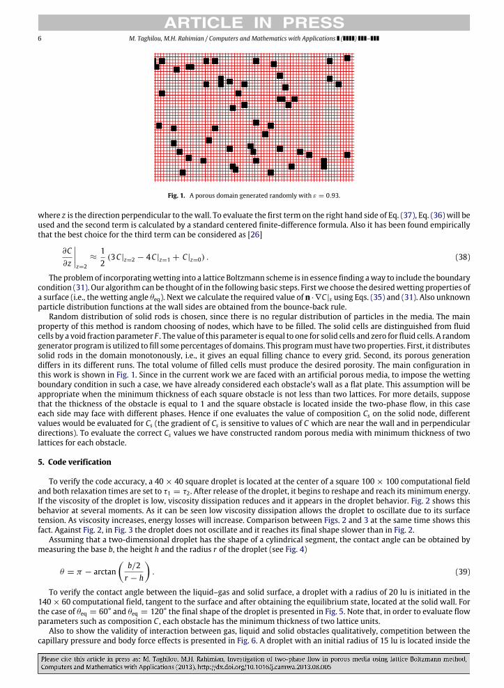
Fig. 1. A porous domain generated randomly with ε = 0.93.

where z is the direction perpendicular to thewall. To evaluate the first term on the right hand side of Eq. (37), Eq. (36) will beused and the second term is calculated by a standard centered finite-difference formula. Also it has been found empiricallythat the best choice for the third term can be considered as [26]

∂C∂z

z=2

≈12

(3C |z=2 − 4C |z=1 + C |z=0) . (38)

The problemof incorporatingwetting into a lattice Boltzmann scheme is in essence finding away to include the boundarycondition (31). Our algorithm can be thought of in the following basic steps. Firstwe choose the desiredwetting properties ofa surface (i.e., the wetting angle θeq). Next we calculate the required value of n ·∇C |s using Eqs. (35) and (31). Also unknownparticle distribution functions at the wall sides are obtained from the bounce-back rule.

Random distribution of solid rods is chosen, since there is no regular distribution of particles in the media. The mainproperty of this method is random choosing of nodes, which have to be filled. The solid cells are distinguished from fluidcells by a void fraction parameter F . The value of this parameter is equal to one for solid cells and zero for fluid cells. A randomgenerator program is utilized to fill somepercentages of domains. This programmust have twoproperties. First, it distributessolid rods in the domain monotonously, i.e., it gives an equal filling chance to every grid. Second, its porous generationdiffers in its different runs. The total volume of filled cells must produce the desired porosity. The main configuration inthis work is shown in Fig. 1. Since in the current work we are faced with an artificial porous media, to impose the wettingboundary condition in such a case, we have already considered each obstacle’s wall as a flat plate. This assumption will beappropriate when the minimum thickness of each square obstacle is not less than two lattices. For more details, supposethat the thickness of the obstacle is equal to 1 and the square obstacle is located inside the two-phase flow, in this caseeach side may face with different phases. Hence if one evaluates the value of composition Cs on the solid node, differentvalues would be evaluated for Cs (the gradient of Cs is sensitive to values of C which are near the wall and in perpendiculardirections). To evaluate the correct Cs values we have constructed random porous media with minimum thickness of twolattices for each obstacle.

5. Code verification

To verify the code accuracy, a 40 × 40 square droplet is located at the center of a square 100 × 100 computational fieldand both relaxation times are set to τ1 = τ2. After release of the droplet, it begins to reshape and reach its minimum energy.If the viscosity of the droplet is low, viscosity dissipation reduces and it appears in the droplet behavior. Fig. 2 shows thisbehavior at several moments. As it can be seen low viscosity dissipation allows the droplet to oscillate due to its surfacetension. As viscosity increases, energy losses will increase. Comparison between Figs. 2 and 3 at the same time shows thisfact. Against Fig. 2, in Fig. 3 the droplet does not oscillate and it reaches its final shape slower than in Fig. 2.

Assuming that a two-dimensional droplet has the shape of a cylindrical segment, the contact angle can be obtained bymeasuring the base b, the height h and the radius r of the droplet (see Fig. 4)

θ = π − arctan

b/2r − h

. (39)

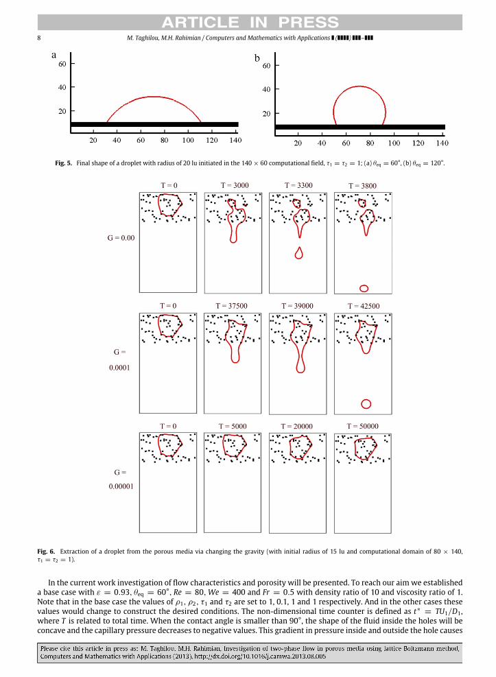
To verify the contact angle between the liquid–gas and solid surface, a droplet with a radius of 20 lu is initiated in the140 × 60 computational field, tangent to the surface and after obtaining the equilibrium state, located at the solid wall. Forthe case of θeq = 60° and θeq = 120° the final shape of the droplet is presented in Fig. 5. Note that, in order to evaluate flowparameters such as composition C , each obstacle has the minimum thickness of two lattice units.

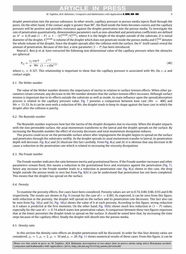
Also to show the validity of interaction between gas, liquid and solid obstacles qualitatively, competition between thecapillary pressure and body force effects is presented in Fig. 6. A droplet with an initial radius of 15 lu is located inside the

M. Taghilou, M.H. Rahimian / Computers and Mathematics with Applications ( ) – 7

Fig. 2. Relaxation of square droplet at the center of computational field with υ = 0.0333 (τ1 = τ2 = 0.1).

Fig. 3. Relaxation of square droplet at the center of computational field with υ = 0.3333 (τ1 = τ2 = 1).

Fig. 4. Geometrical measurement of the contact angle.

porous media with a porosity of 0.93 which is put in the computational domain of 80 × 140. Also the value of body force iscontrolled by changing the value of gravitational acceleration.

As it is expected, by decreasing the body force, the dropletwill be extracted slowly and finally it will stick in the substrate.

6. Results and discussion

In the problem of droplet impact on the permeable surface and its penetration into porous media nine non-dimensionalparameters are considered [6]. These are the Reynolds number Re = ρ1u1D1/µ1; the porosity ε = Vpores/Vtotal; the Froudenumber Fr = u2

1/gR1; the Darcy number Da = K/R21; the Weber number We = ρu2

1R1/σ12; the contact angle θeq; densityratio ρr = ρ1/ρ2; viscosity ratio υr = ν1/ν2 and characteristics of the porous medium structure α = dpores/dp.

8 M. Taghilou, M.H. Rahimian / Computers and Mathematics with Applications ( ) –

Fig. 5. Final shape of a droplet with radius of 20 lu initiated in the 140 × 60 computational field, τ1 = τ2 = 1; (a) θeq = 60°, (b) θeq = 120°.

Fig. 6. Extraction of a droplet from the porous media via changing the gravity (with initial radius of 15 lu and computational domain of 80 × 140,τ1 = τ2 = 1).

In the current work investigation of flow characteristics and porosity will be presented. To reach our aim we establisheda base case with ε = 0.93, θeq = 60°, Re = 80,We = 400 and Fr = 0.5 with density ratio of 10 and viscosity ratio of 1.Note that in the base case the values of ρ1, ρ2, τ1 and τ2 are set to 1, 0.1, 1 and 1 respectively. And in the other cases thesevalues would change to construct the desired conditions. The non-dimensional time counter is defined as t∗ = TU1/D1,where T is related to total time. When the contact angle is smaller than 90°, the shape of the fluid inside the holes will beconcave and the capillary pressure decreases to negative values. This gradient in pressure inside and outside the hole causes

M. Taghilou, M.H. Rahimian / Computers and Mathematics with Applications ( ) – 9

droplet penetration into the porous substance. In other words, capillary pressure in porous media injects fluid through thepores. On the other hand, if the contact angle is greater than 90°, the fluid inside the holes becomes convex and the capillarypressure will be positive and provides resistance against the droplet penetration into the porous media. To investigate therate of penetration quantitatively, dimensionless parameters such as non-absorbed and penetration coefficients are definedas: h∗

= h/D and (1 − P) = 1 − (V outside1 /V total

1 ), where h is the height of the droplet outside of the substrate, D is initialdiameter of the droplet, V outside

1 is volume of the droplet which does not penetrate inside the porousmedia and V total1 denotes

the whole volume of the droplet. Since the droplet spreads after the collision with the surface, the h∗ itself cannot reveal theamount of penetration. Because of this fact, a new parameter (1 − P) has been introduced.

Neyval C. Reis Jr et al. have extracted the following non-dimensional value of the capillary pressure when the obstaclesare spherical

Pca =c3α

cos θ

Weε3/2

(1 − ε)Da1/2, (40)

where c3 = 0.327. This relationship is important to show that the capillary pressure is associated with We, Da, ε, α andcontact angle.

6.1. The Weber number

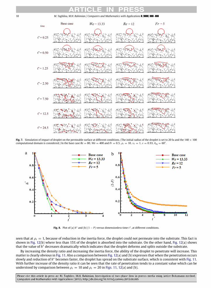
The value of the Weber number denotes the importance of inertia in relation to surface tension effects. When other pa-rameters retain constant, any decrease in theWe number denotes that the surface tension effect increases. Although surfacetension is important due to its effects outside the substrate as well as inside, its main influence upon the spread/absorptionprocess is related to the capillary pressure value. Fig. 7 presents a comparison between base case (We = 400) andWe = 13.33. As it can be seen with a reduction ofWe, the droplet tends to keep its shape against the base case in which thedroplet after the collision is patchy.

6.2. The Reynolds number

The Reynolds number expresses how fast the inertia of the droplet dissipates due to viscosity. When the droplet impactswith the non-permeable surface, the axial momentum transforms to the lateral and the droplet spreads on the surface. Byincreasing the Reynolds number the effect of viscosity decreases and total momentum dissipation reduces.

This process could occur on the permeable surface where after impingement the droplet begins to spread on the surfaceand penetrates through the substrates swiftly. As the droplet spreads its axial momentum transfer to lateral, its penetrationdepth will decrease. Fig. 8(a) and (b) illustrate this fact carefully. From Fig. 8(a) and (b) it is obvious that any decrease in Recause a reduction in the penetration rate which is related to increasing the viscosity dissipations

6.3. The Froude number

The Froude number indicates the ratio between inertia and gravitational forces. If the Froude number increases and otherparameters remain fixed, this means a reduction in the gravitational force and resistance against the penetration (Fig. 7),hence any increase in the Froude number leads to a reduction in penetration rate. Fig. 8(a) shows in this case, the dropheight outside the porous tends to zero but from Fig. 8(b) it can be understood that penetration has not been completed.This means that the droplet has spread on the surface.

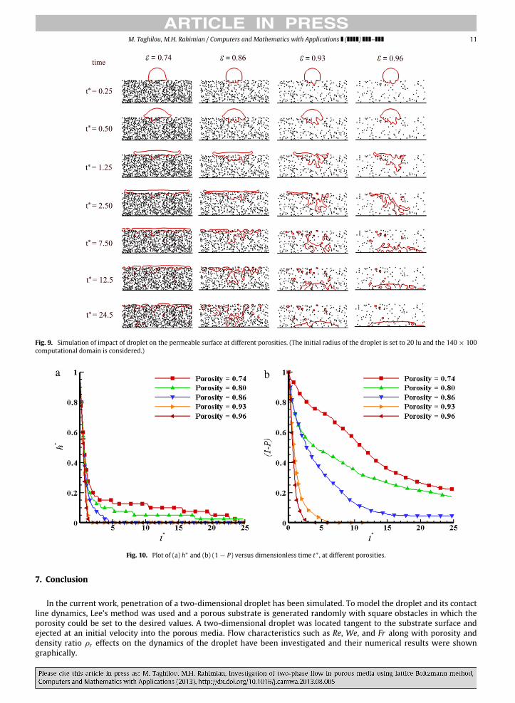
6.4. Porosity

To examine the porosity effects, five cases have been considered. Porosity values are set to 0.74, 0.80, 0.86, 0.93 and 0.96respectively. The results are shown in Fig. 9 (except for the case of ε = 0.80). As expected, it can be seen from this figure,with reduction in the porosity, the droplet will spread on the surface and its penetration rate decreases. This fact also canbe seen from Fig. 10(a) and (b). Fig. 10(a) shows the value of h at each porosity. According to this figure, strong reductionin h values is predicted at the first moments. On the other hand, Fig. 10(b) shows much less reduction in (1 − P) values,especially for the case of ε = 0.74 which states low penetration values. A comparison between these two figures expressesthat at the lower porosities the droplet tends to spread on the surface. It should be noted here that, by increasing the timesteps because of the capillary effect, finally the droplet will absorb into the porous media.

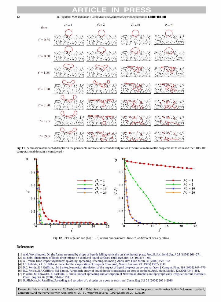
6.5. Density ratio

In this section the density ratio effects on droplet penetration will be discussed. In order for this four density ratios areconsidered: ρr = 1, ρr = 2, ρr = 10 and ρr = 20. Fig. 11 shows numerical results of these cases. From this figure, it can be

10 M. Taghilou, M.H. Rahimian / Computers and Mathematics with Applications ( ) –

Fig. 7. Simulation of impact of droplet on the permeable surface at different conditions. (The initial radius of the droplet is set to 20 lu and the 140 × 100computational domain is considered.) In the base case Re = 80,We = 400 and Fr = 0.5, ρr = 10, υr = 1, ε = 0.93, θeq = 60°.

Fig. 8. Plot of (a) h∗ and (b) (1 − P) versus dimensionless time t∗ , at different conditions.

seen that at ρr = 1, because of reduction in the inertia force, the droplet could not permeate into the substrate. This fact isshown in Fig. 12(b) where less than 15% of the droplet is absorbed into the substrate. On the other hand, Fig. 12(a) showsthat the value of h∗ decreases dramatically which indicates that the droplet deforms and splits outside the substrate.

By increasing the density ratio and increasing the inertia force, the ability of the droplet to penetrate will increase. Thismatter is clearly obvious in Fig. 11. Also a comparison between Fig. 12(a) and (b) expresses that when the penetration occursslowly and reduction of h∗ becomes faster, the droplet has spread on the substrate surface, which is consistent with Fig. 11.With further increase of the density ratio it can be seen that the rate of penetration tends to a constant value which can beunderstood by comparison between ρr = 10 and ρr = 20 in Figs. 11, 12(a) and (b).

M. Taghilou, M.H. Rahimian / Computers and Mathematics with Applications ( ) – 11

Fig. 9. Simulation of impact of droplet on the permeable surface at different porosities. (The initial radius of the droplet is set to 20 lu and the 140 × 100computational domain is considered.)

Fig. 10. Plot of (a) h∗ and (b) (1 − P) versus dimensionless time t∗ , at different porosities.

7. Conclusion

In the current work, penetration of a two-dimensional droplet has been simulated. To model the droplet and its contactline dynamics, Lee’s method was used and a porous substrate is generated randomly with square obstacles in which theporosity could be set to the desired values. A two-dimensional droplet was located tangent to the substrate surface andejected at an initial velocity into the porous media. Flow characteristics such as Re, We, and Fr along with porosity anddensity ratio ρr effects on the dynamics of the droplet have been investigated and their numerical results were showngraphically.

12 M. Taghilou, M.H. Rahimian / Computers and Mathematics with Applications ( ) –

Fig. 11. Simulation of impact of droplet on the permeable surface at different density ratios. (The initial radius of the droplet is set to 20 lu and the 140×100computational domain is considered.)

Fig. 12. Plot of (a) h∗ and (b) (1 − P) versus dimensionless time t∗ , at different density ratios.

References

[1] A.M. Worthington, On the forms assumed by drops of liquids falling vertically on a horizontal plate, Proc. R. Soc. Lond. Ser. A 25 (1876) 261–271.[2] M. Rein, Phenomena of liquid drop impact on solid and liquid surfaces, Fluid Dyn. Res. 12 (1993) 61–93.[3] A.L. Yarin, Drop impact dynamics: splashing, spreading, receding, bouncing, Annu. Rev. Fluid Mech. 38 (2006) 159–192.[4] I.D. Roberts, R.F. Griffiths, A model for the evaporation of droplets from sand, Atmos. Environ. 29 (1995) 1307–1317.[5] N.C. Reis Jr., R.F. Griffiths, J.M. Santos, Numerical simulation of the impact of liquid droplets on porous surfaces, J. Comput. Phys. 198 (2004) 747–770.[6] N.C. Reis Jr., R.F. Griffiths, J.M. Santos, Parametric study of liquid droplets impinging on porous surfaces, Appl. Math. Model. 32 (2008) 341–361.[7] P. Alam, M. Toivakka, K. Backfolk, P. Sirviö, Impact spreading and absorption of Newtonian droplets on topographically irregular porous materials,

Chem. Eng. Sci. 62 (2007) 3142–3158.[8] N. Alleborn, H. Raszillier, Spreading and sorption of a droplet on a porous substrate, Chem. Eng. Sci. 59 (2004) 2071–2088.

M. Taghilou, M.H. Rahimian / Computers and Mathematics with Applications ( ) – 13

[9] N. Alleborn, H. Raszillier, Spreading and sorption of droplets on layered porous substrates, J. Colloid Interface Sci. 280 (2004) 449–464.[10] X. Shan, H. Chen, Lattice Boltzmann model for simulating flows with multiple phases and components, Phys. Rev. E 47 (3) (1993) 1815–1819.[11] X. He, S. Chen, R. Zhang, A Lattice Boltzmann scheme for incompressible multiphase flow and its application in simulation of Rayleigh–Taylor

instability, J. Comput. Phys. 152 (1999) 642–663.[12] S. Mukherjee, J. Abraham, Investigations of drop impact on dry walls with a lattice-Boltzmann model, J. Colloid Interface Sci. 312 (2007) 341–354.[13] T. Lee, Effects of incompressibility on the elimination of parasitic currents in the lattice Boltzmann equation method for binary fluids, Comput. Math.

Appl. 58 (2009) 987–994.[14] T. Lee, L. Liu, Lattice Boltzmann simulations of micron-scale drop impact on dry surfaces, J. Comput. Phys. 229 (2010) 8045–8063.[15] T. Lee, C.L. Lin, A stable discretization of the lattice Boltzmann equation for simulation of incompressible two-phase flows at high density ratio,

J. Comput. Phys. 206 (2005) 16–47.[16] A.J. Wagner, The origin of Spurious velocities in lattice Boltzmann, Internat. J. Modern Phys. B 17 (2003) 193–196.[17] D. Jacqmin, An energy approach to the continuum surface tension method, AIAA 96-0858, in: Proceedings of the 34th Aerospace Sciences Meeting

and Exhibit, American Institute of Aeronautics and Astronautics, Reno.[18] A.L. Kupershtokh, New method of incorporating a body force term into the lattice Boltzmann equation, in: Proc. 5th International EHD Workshop,

University of Poitiers, Poitiers, France, 2004, pp. 241–246.[19] A.L. Kupershtokh, Criterion of numerical instability of liquid state in LBE simulations, Comput. Math. Appl. 59 (2010) 2236–2245.[20] A.L. Kupershtokh, D.A. Medvedev, D.I. Karpov, On equations of state in a lattice Boltzmann method, Comput. Math. Appl. 58 (2009) 965–974.[21] D. Chiappini, G. Bella, S. Succi, F. Tosch, S. Ubertini, Improved Lattice Boltzmann without parasitic currents for Rayleigh–Taylor instability, Commun.

Comput. Phys. 7 (2010) 423–444.[22] Q. Lou, Z.L. Guo, C.G. Zheng, Some fundamental properties of lattice Boltzmann equation for two phase flow, CMES Comput. Model. Eng. Sci. 76 (3)

(2011) 175–188.[23] Q. Lou, Z.L. Guo, B.C. Shi, Effects of force discretization on mass conservation in lattice Boltzmann equation for two-phase flows, Europhys. Lett. 99

(2012) 64005.[24] T. Lee, L. Liu, Wall boundary conditions in the lattice Boltzmann equation method for nonideal gases, Phys. Rev. E 78 (2008) 017702.[25] A.J. Briant, A.J. Wagner, J.M. Yeomans, Lattice Boltzmann simulations of contact line motion, I. Liquid-gas systems, Phys. Rev. E 69 (2004) 031602.[26] Y.Y. Yan, Y.Q. Zu, A lattice Boltzmannmethod for incompressible two-phase flows on partial wetting surface with large density ratio, J. Comput. Phys.

227 (2007) 763–775.