Investor Behavior and Volatility of Futures Market: A

Front. Bus. Res. China 2011, 5(3): 512–536 DOI 10.1007/s11782-011-0143-2

Received December 10, 2010

Yun Wang ( ) Center for Non-Traditional Security Studies, Hubei Key Research Institute of Humanities and Social Science, Huazhong Unversity of Science & Technology, Wuhan 430074, China E-mail: [email protected] Zongcheng Zhang Center for Non-Traditional Security Studies, Hubei Key Research Institute of Humanities and Social Science, Huazhong University of Science & Technology, Wuhan 430074, China E-mail: [email protected] Renhai Hua School of Finance, Nanjing University of Finance & Economics, Nanjing 210037, China E-mail: [email protected]

RESEARCH ARTICLE

Yun Wang, Zongcheng Zhang, Renhai Hua

Investor Behavior and Volatility of Futures Market: A Theory and Empirical Study Based on the OLG Model

© Higher Education Press and Springer-Verlag 2011

Abstract Investor trading behaviors are always an important issue in behavioral finance and market supervision. This study examines the relationship between investor behavior and future market volatility. We first introduce a two-period OLG model into the futures market, and develop an investor behavior model based on future contract price. We then extend the model to two scenarios: complete and incomplete information. We provide the equilibrium solution, and develop two hypotheses, which are tested with cuprum tick data in Shanghai Futures Exchange (SHFE). Empirical results show that the two-period OLG model for future market is consistent with the market situation in China. More specifically, investors with sufficient information such as institutional investors usually adopt the contrarian trading strategy, whereas investors with insufficient information, e.g., individual investors, usually adopt the momentum trading strategy. These findings reveal that investor behaviors in the Chinese futures market are different from those of in the Chinese stock market.

Investor Behavior and Volatility of Futures Market 513

Keywords investor behavior, overlapping generation model, momentum trading, contrarian trading

1 Introduction and Literature Review

The momentum effect and contrarian effect of investor behaviors have been well demonstrated in stock market. Jegadeesh and Titman (1993) first discovered the momentum effect of investors in the stock market: selling low-return stocks in the past 3, 6, 9 and 12 months and buying high-return ones in the same period among public companies listed in New York Stock Exchange (NYSE) and American Stock Exchange (AMEX) from 1965 to 1989. They built a winner group and a loser group respectively, and developed 16 trading strategies by cross-mating. Their results showed that the strategy of selling the “winners” in the last 6 months and buying the “losers” concurrently gained a monthly average return of approximately 1%. Almost all the strategies could produce profit, and the excess return remained significant even after risk adjustment or accounting for all sales charges and expenses. Studies of Chan et al. (1996), Campell (1993) and Shiller (1981) all confirmed the existence of momentum effect and contrarian effect. A number of Chinese studies also examined the momentum effect in stock market, such as Wang and Zhao (2001). It is commonly argued that as an emerging market, the Chinese securities market is different from western ones on its contrarian strategy. Momentum effect is not significant in the Chinese stock market, while the mid- and long-term contrarian effect is more pronounced. China’s futures market, however, is greatly different from the stock market. It remains unclear whether similar pattern exists in the futures market in China. Little research has examined the investor behavior and volatility in future markets. This is mainly due to the absence of theoretical models based on futures market, which is the key problem to be solved in this study.

Based on the assumption that investors have representativeness bias and conservatism bias, Barberis, Shleifer, and Vishny (1998) (BSV) show that investors’ under-reaction to single unexpected return leads to continuation under conservatism bias, while their over-reaction to positive returns leads to the long-term reversals under representativeness bias. The irrationality of investors described in their study can be explained by three Markov processes and the investor state transition abided by the Bayesian Law. Daniel, Hirshleifer, and Suhramanyam (1998) (DHS) assumed that there were two types of investors in securities market, i.e., informed and non-informed investors. Investors’ overconfidence in private information and self-attribution bias of public

514 Yun Wang, Zongcheng Zhang, Renhai Hua

information jointly lead to short-term continuation and a price divergence from the fundamental value, while the divergence would fade away in the long term and long-term reversal would occur. The irrationality of investors mainly originates in the process by which information miners respond to and spread information, and the momentum trader could only affect trading volume of securities. Harrison and Stein (1999) (HS) assumed that there were two types of irrational investors: information miner and momentum trader. The former is prone to under-reaction while the latter is prone to over-reaction, which leads to continuation and long-term reversal, respectively. Loss-Aversion and House Money effect refer to the hypotheses that investors’ risk aversion reduced as the prices of securities raise, which leads to further increase of security prices; investors’ risk aversion increases as prices decrease, which leads to further decrease of security prices. Based on these two hypotheses, Barberis, Huang, and Santos (2001) (BHS) developed an equilibrium model which captures the short-term continuation and long-term reversal phenomena.

Nevertheless, the above mentioned investor behavior models (BSV, DHS, HS, and BHS) all rely too heavily on theoretical assumptions, neglecting investors’ behavior deviation in real life. Under such a circumstance, the overlapping generations model (OLG) used in macroeconomics is introduced into the study of investor trading behavior for two obvious advantages: First, it provides a dynamic research framework under which investors’ trading behavior and asset price volatility could be closely related. Second, the two-period OLG model describes the simplest dynamic economic situation, and it can be extended to three-period or even infinite period situations. Therefore, a growing number of researchers have adopted OLG model in their stock market studies. For example, Shiller (1981) firstly introduced OLG model to the analysis of stock market volatility. De Long et al. (1990a) put forward a simple two-period OLG model for securities market, in which the unpredictability of noise traders’ random beliefs could affect the price and obtain high expected returns, resulting in market risk and leading to price divergence from fundamental value. The author thus believed that the model is able to explain a series of market anomalies. Although it has been generally assumed in rational speculating analysis that the noise traders restrain the market volatility, De Long et al. (1990b) found, based on his four-period OLG model, that if noise traders choose positive feedback strategy, namely, to buy upon price increasing and to sell upon price decreasing, they buy prior to the noise. Moreover, if rational investors adopt positive feedback strategy earlier, the volatility in fundamental surface would be aggravated. The empirical evidence supported the above assumptions. Campbell


and Kyle (1991) and Wang (1993, 1994) also conducted similar studies by establishing the finitely-lived agent model.

Furthermore, Spiegel (1998) found that the stock price volatility could not be fully explained by standard dividend discount model, and thus introduced the OLG model to explain stock price volatility. His model consists of a random supply of risky asset and finitely-lived agents trading in conforming asset environment. The analysis shows that there are a total of 2K equilibriums when K types of securities are traded, and the highly volatile equilibrium has unique characteristics compared with other types of equilibriums. Based on Spiegel’s (1998) model, Mashiro (2008) built a more complicated OLG model by employing the precondition of heterogeneously informed agents. Mashiro analyzed situations in which agents are fully informed, not informed or partly informed, and he found that less informed agents tend to employ momentum trading while better informed agents apply contrarian strategies. The trading volume is inverted-u-shaped due to information precision and is positively correlated with absolute price. Finally, precise information does not only increase the volatility, but also is associated with stock return in high volatility and is strongly associated with volatility equilibrium. The author believed that the volatility equilibrium is not likely to deviate once it is produced. Although the equilibrium is not the Pareto optimal one, the sub-optimal and steady equilibrium is common in real life.

Researchers in China also conducted some studies on stock market based on the OLG model. For example, Kong (2009) built a two-period OLG model and introduced traders with subjective belief bias into capital markets to examine their impact on asset price volatility by equilibrium analysis. It was found that the belief biases and learning ability of noise traders, the market status, market dominance and risk aversion degree all have impacts on assets fluctuations but in different ways. The consequent empirical analysis partially confirmed this conclusion. According to the testing results, stock market volatility in China is mainly affected by investor sentiment and market status, and institutional investors stabilize the market to some extent.

This paper intends to build a model and empirical framework of investor behavior on futures market. The idea is to improve on the OLG model for stock market proposed by De Long (1990b), Spiegel (1998) and Mashiro (2008) from such perspectives as the precondition assumption, parameter setup and the maximization condition, so as to make the model suitable for the futures market in practice. Five related propositions and two hypotheses are proposed based on the model. Therefore, the model proposed by this paper is different from above mentioned theoretical models.


The main contributions of this study are: 1) it takes the lead to introduce the OLG model into futures market and builds a two-period investor behavior OLG model, which is extended to full and partial information situation to get the equilibrium respectively; 2) it conducts empirical studies for the two assumptions based on the five propositions of the model with intraday data of futures contracts listed in the future market of Chinese mainland. The empirical findings partly confirm the deductions of the model that perfect informed futures investors represented by institutional investors generally take contrarian strategies and less informed investors represented by individual investors behave as trend-followers.

2 A Two-Period OLG Model Based on Futures Market

Based on the findings of Spiegel (1998) and Mashiro (2008), this paper attempts to build the OLG Model based on futures market, and to analyze the relationship between investor behavior and futures volatility in the framework.

Suppose there are K future investors in the market and that a riskless bond pays r units per period. In period t, the futures contract comes up with a risk premium Pt and { }1 2 3, ,t t t t ntP P P P P= ⋅ ⋅ ⋅ . Designate tδ is the shock of Pt,

following a random walk process N(0, δ∑ ). Then,

1 .t t tP P δ−= + (1)

Therein the risk premium is not described by spot price because the proposition whether futures prices are unbiased estimates of spot price is still controversial among scholars. Leuthold (1974), Martin and Garcia (1981), Hokkio and Rush (1989), and Chen and Zheng (2007), believed that arbitrageurs in futures market inevitably require reasonable risk returns, namely, risk premium Pt in this paper.

In microstructure model of futures market, assume the futures contract supply as Nt, then }{ 1 2,t t t ktN N N N= ⋅ ⋅ ⋅ . Designate tη as the shock of supply Nt,

following a random walk process N(0, η∑ ) , then

1 .t t tN N η−= + (2)

Therefore, future contract price F is mainly determined by its supply and risk premium Pt. We assume that the future contract price-F is controlled by supply Nt and risk premium Pt, and Set two state vectors A and B and a matrix A, B~ .K K× A represents the spot change of the futures contracts supply and B


represents the spot change of future contracts’ risk premium, then .t t tF AN BP= + (3)

The supply is the seller of futures contracts, and the demand is the buyer of the futures contracts, thus where supply equals to demand is market clearing point. The price at this point is market clearing price. The above tF refers to the market clearing price of futures contract. Set Xt as investors’ demand of futures contract, then { }1 2 3, ,t t t t ktX X X X X= ⋅ ⋅ ⋅ , where K represents the Kth futures

contracts. Here we introduce two critical assumptions as the theoretical basis of the model.

Assumption 1 There exists only one tiny continuum in each unit trading of futures investors, that is, each trader acts as a price taker, thus individuals are unable to affect the price.

Assumption 2 Futures investors are more risk-seeking than stock investors. The utility U of the final consumption of futures traders in period t +1 follows an exponential utility function; the risk aversion coefficient is θ ; the function is

(2 )WU e θ−= − . Under the above two assumptions, we build the Overlapping Generation (OLG)

model based on futures market. Suppose that futures investors live for two periods, born in period t and entering into futures market, and dying at the end of period t +1 and exiting. Investors demand for wealth maximization with risk preference. They hold two types of assets: one is riskless bond denoted as b and the other is futures contract as risky assets denoted as F. Then for an investor i, his wealth in period t is as below:

( ) ( ) ( )t t t tW i X i F b i= + . (4)

Considering the risk premium of futures contract and returns of riskless bonds, the investor’s final wealth in period t + 1 is

[ ]1 1 1( ) ( ) (1 ) ( )t t t t tW i X i F P r b i+ + += + + + , (5)

where, Ft+1 stands for price of the futures contract in period t +1, Pt+1 denotes risk premium of the futures contract in the period t +1, and r denotes riskless interest rate. Plugging Equation (4) into Equation (5) simplifies to:

[ ]1 1 1( ) ( ) (1 ) ( )t t t t t t tW i X i F F P rF r W i+ + += − + − + + . (6)

Substituting Equation (3) into Equation (6) and eliminating Ft+1 and Ft yields

[ ]1 1 1 1( ) ( ) (1 ) ( )t t t t t t t tW i X i A B P rF r W iη δ δ+ + + += + + + − + + . (7)


The above equation is thus converted into a question for optimization solution. As assumed in Assumption 2, the investor seeks to maximize his expected utility Ut+1, namely, to maximize the equation 1(2 )

1( ) tWtE U e θ +−+ = − . According to the

deductions of De Long (1990), the maximization of 1tU + is equal to the maximization of the following formula: 1 10.5 .t tW Wθ+ +− Σ (8)

Expanding the formula (8) gives

[ ] { }max (1 ) 0.5 ' ( ) ' ( ) .T Tt t t t t tXt

X P rF r W X A A I B I B Xη δθ− + + − Σ + Σ + (9)

Calculate the first-order condition of the above formula. Differentiating the above function matrix and simplifying it yields

.( ) ( )

t tt T T

P rFX

A A I B I Bη δθ−

=⎡ ⎤Σ + + Σ +⎣ ⎦

(10)

Substitute Equation (3) into Equation (11):

.( ) ( )

t t tt T T

P rAN rBPX

A A I B I Bη δθ− −

=⎡ ⎤Σ + + Σ +⎣ ⎦

(11)

According to Assumption 1, there exists only one tiny continuum in each unit trading of futures investors, which has no effect on price. Therefore, under market clearing equilibrium, the equilibrium price shall be the same as the price when futures contract supply equals the demand, namely,

.t tN X= (12)

Calculate the second order condition of Equation (11):

( ) ( ) 0.T TrA A A I B I Bη δθΣ + + + Σ + = (13)

Futures risk premium is in inverse correlation with interest rate of riskless bonds. The higher the interest rate of riskless bonds is, the fewer the futures traders there are, and vice versa. We assume the two variables have the relationship as below:

1 .B Ir

= (14)

Substituting Equation (15) into Equation (14) to obtain the expression of state vector A:

21 0.T r rA A A

rη δθ+⎛ ⎞Σ + + Σ =⎜ ⎟

⎝ ⎠ (15)


Accordingly, the above section built a simple two-period overlapping generation model based on futures market and produced the first-order and second-order conditions. Some relevant propositions will be deducted in the following section. According to the above solutions and referring to the researches of Spiegel (1998), Matanabe (2008) and Kong (2009), the following propositions are obtained.

Proposition 1 Demand for futures contract is affected by risk premium and its price, and it is positively correlated with the risk premium and negatively correlated with the price.

Proof: see the Appendix. Proposition 2 Futures contract state vector A is symmetric, with the

following expression:

11 12 2 2

1 2 2 21 1 1 .2 4

r r rArη η η δ ηθ θ

− −− −⎡ ⎤+⎛ ⎞ ⎛ ⎞= − Σ + Σ − Σ Σ Σ⎢ ⎥⎜ ⎟ ⎜ ⎟

⎝ ⎠ ⎝ ⎠⎢ ⎥⎣ ⎦ (16)

The futures price volatility may exist even in the absence of risk premium. Proof: see the Appendix. Proposition 3 The price volatility of futures contract is affected by riskless

interest rate r, risk aversion coefficient θ, state vector A and volatility matrix of risk premium δΣ , and follows the following expression:

2

1 11( ) ( ) .T Tr rA Arη δθ

− −+⎛ ⎞Σ = − − Σ⎜ ⎟⎝ ⎠

(17)

The four variables have complicated nonlinear relation. Proof: see the appendix.

3 Extension of the Model: Considering Complete and Partial Information Cases

In the previous section, heterogeneous information was not taken into consideration. Futures investors were assumed to be uninformed, which is rarely the case in real life. Now let’s discuss two situations: (1) futures investors are fully informed; (2) futures investors are partially informed. First, an information variable is added into Equation (3) hereinbefore to build a linear expression of price volatility including the two situations. 1 1 2 1 2 1 .t t t t tF A N A B P B Cη δ− += + + + + (18)

The above equation is actually the extension and conversion of Equation (3) by adding different variable coefficients. We need to discuss the steady


equilibrium of these coefficients as time is invariant. As for the returns and utility of investors, assume Qt+1 as the excess return for each futures contract. Extending the above Equation (5), we have the following expression:

1 1( ) ( ) (1 ) ( ).t t t tW i X i Q r W i+ += + + (19)

1 1 1 (1 ) .t t t tQ F P r F+ + += + − + (20)

Equation (20) represents that the investor i’s returns in the 2nd period equal to his excess returns in the 2nd period plus the wealth discount in the 1st period; while Equation (21) shows that the investor i’s excess returns of each contract equal to the price in the 2nd period plus the risk premium and minus price discount in the 1st period, which is consistent with Equation (5), (6) and (7). The following sections are the discussion for the two situations. 3.1 Fully-Informed Futures Investors In this situation, investors may forecast accurately the shock that would occur

with the information they hold and hence 1 2A A A= = , 1 21B B Ir

= = and

0c = . Substituting the two conditions into Equation (21) and simplifying it yields

1 .t t tF AN Pr

= + (21)

Substituting Equation (25) in Equation (24) and simplifying it yields

1 1 2 11 .t t t t tQ A P rFr

η δ+ + + += + + − (22)

This is the expression of investors’ excess returns in fully-informed cases. Let the information set of investor i be { }, , , 1, , , ,t i t i t i t t tF P Nδ η −ℜ = . According to

Assumption II, the utility maximization is 1(2 ),max tW

t iE e θ +−⎡ ⎤− ℜ⎣ ⎦ which can

be converted to into the solution for the following maximization.

1, , ,max 0.5 1, .t i t i t iE W Var Wt iθ+⎡ ⎤ ⎡ ⎤ℜ − + ℜ⎣ ⎦ ⎣ ⎦ (23)

No further explanation on the proof process which is similar to above. The first-order condition is obtained.

11 , 1 ,

1, ( )t t i t t iXt i Var Q F E Q Fθ

−+ +

⎡ ⎤= ⎣ ⎦


11

1 ( ) ( ).T Tt tA A B B P rFη δθ

−+= Σ + Σ − (24)

The second-order condition may be met if 1 ,( )t t iVar Q F+ is positive definite matrix in fully-informed cases.

21 0.rA A Arη δθ

Σ + + Σ = (25)

Observing the above equation one may get Proposition 4. Proposition 4 In fully-informed cases, the price volatility of futures contract

is affected by riskless interest rate r, risk aversion coefficient θ, state vector A and volatility matrix of risk premium δΣ , and it is inversely associated with the volatility of risk premium. Its vector matrix follows the following equation:

1 1 12

1 .r A A Arη δθ

− − −Σ = − − Σ (26)

Proof: see the appendix. Comparing the above equation and Equation (20) one can find that the switch

from none information to full information can be realized by changing the state vector A matrix. 3.2 Partially-Informed Futures Investors This is the most complicated case in the paper. As futures traders receive different information in different periods, futures supply coefficient A1 and supply shock coefficient A2 are different respectively, so are risk premium

coefficients B1 and B2. Substituting the two conditions 1 2A A≠ , 1 21B I Br

= ≠

and 0c = into Equation (22) simplifies to:

( )11 1 2 1 2 2

1 .t t t tFt A N P B B Ar

δ η−− += + + + (27)

The investor’s excess return under the information set ,t iℜ in period t+1 is

1 1

1 1 2 2 1 2 2 2 11

1 1 1 2 2

( ) ( )

( ) .t t t t

t t t t

Q A A I B B A A

B I A F B P rF

δ η η

δ δ

− −+ + +

−+ +

= − + +

+ + − + + −

(28)

The maximization, similar to that in fully-informed cases, needs to be solved from Equation (28). Refer to Appendix for detailed calculation. The difference is the first-order condition obtained:


11 , 1 ,

1 12 2 1 1 2 2 1 1 2 2

1 1 12 2 1 2 2 1 2 2

11 1 2 2 1 , 1

1, ( )

1 ( ( ) ( )

) ( ) ( )

( ) .

t t i t t i

T Ti

Tt t

t t i t t

Xt i Var Q F E Q F

A A B I A A B B I A A B

B B A A I B B A

B I A A B E P rF

η

δ

θ

θδ η

δ

−+ +

− −

− − −+

−+ +

⎡ ⎤= ⎣ ⎦

= Σ + + − Σ + −

+ Σ − +

⎡ ⎤+ + − ℜ + −⎣ ⎦

(29)

There are so many parameters that it needs to be discussed case by case, which is out of the scope of this paper. The second order condition is given herein and can be simplified to

1 1.t t

rAδ η+Σ = Σ + (30)

Proposition 5 is obtained according to the above equation. Proposition 5 In partial-informed cases, the futures risk premium volatility

1tδ +Σ is affected by futures price volatility

tηΣ , riskless interest rate r and the

last-period supply state vector A1, and is positively correlated with the three factors.

Proof: see the appendix.

4 Research Design and Data Process

The Two-period OLG Model has been built in the previous sections and extended to the case of full and partial information, drawing five propositions. This section describes our empirical studies and discuss implications of the mathematical model constructed.

Propositions 1, 2 and 3, as we can see, originate from the benchmark model with no information, while Propositions 4 and 5 originate from extension of benchmark model, with full information and no information, respectively. Therefore, Propositions 4 and 5 are developed on the basis of Propositions 1, 2 and 3. Propositions 4 and 5 are most valuable for analyzing the momentum trading and contrarian trading behavior of futures investors in this paper. Hence the empirical section is developed around these two propositions. Due to the lack of direct evidence from prior literature, the empirical section, instead of applying structural estimation, makes some predictions from the model, deduces empirical hypotheses and makes some empirical verification.

To be specific, such four variables as riskless interest rate r, risk aversion coefficient θ, state vector A and volatility matrix of risk premium δΣ are involved in Proposition 4; it shall be noted particularly that in fully-informed cases, the price volatility of futures contract is inversely correlated with the volatility of


risk premium. The higher the volatility of the price, the lower the volatility of the risk premium. Fully-informed investors are more likely to seek for stable risk returns and to trade such contracts; the lower the volatility of the price, the higher the volatility of the risk premium. Fully-informed investors are more likely to seek volatile risk returns and less likely to trade such contracts. Therefore, investors apply contrarian trading strategies, buying stock with low return in the past and selling stock with high return in the past, following “the lowering” instead of “the rising.” Hence, this paper attempts to build a verifiable hypothesis as below:

H1 Fully-informed futures investors can make accurate prediction of future shocks with information in hand and employ contrarian trading strategy.

Such four variables as futures price volatility matrix ,

tηΣ futures risk premium

volatility matrix 1,

tδ +Σ riskless interest rate r and the last-period supply state

vector A1 are involved in proposition 5; it shall be particularly noted that in partially-informed cases, the price volatility of futures contract is positively correlated with risk premium volatility. That is, the higher the price volatility, the higher the risk premium volatility upon the expected returns is requested by investors. Investors are less likely to trade such contracts; the lower the price volatility, the lower the risk premium volatility upon the expected returns is requested by investors. Investors are more likely to trade such contracts. Therefore investors apply trend (momentum) trading strategies to buy stock with high return in the past and sell stock with low return in the past, following “the rising” instead of “the lowering.” Hence, this paper develops another verifiable hypothesis as below:

H2 Partial-informed futures investors can only make predictions of partial shocks in future with information in hand and apply continuation trading strategy.

Upon development of the two hypotheses, proper proxy variables shall be

selected to serve as indexes in empirical analysis. First of all, how to distinguish full information and partial information that investors are to consider. This is not an easy task. Prior literature (such as Wang et al., 2001; Kong, 2009) shows that generally institutional investors are able to get more information than individual investors. Hence in the empirical section we classify investors into two categories: one is institutional investors (with sufficient information or full information) and the other is individual investors (with no information or partial information). Hence, in the empirical section, institutional investors and


individual investor should be distinguished from each other. Then, the trading strategies and returns of the two trading groups in a given period should be analyzed to identify the relevant trading mode.

Data used in this paper were the copper futures tick data in SHFE, collected within a period of 484 trading days from 1 January 2007 to 31 December 2008, with 1 033 980 tick data in total. The tick data included trading direction and provided by WSTOCK. Tick data were used because investor categories such as institutional investors and individual investors could be distinguished by analyzing trading volume. Copper futures contract was used because it is relatively mature and active kind of futures in Chinese futures market, which is commonly used in current empirical studies on futures (Hua et al, 2002). Therefore，it is reasonable to verify investors’ trading behavior in futures market by copper futures contract.

This research used the SAS 9.1.3 program to perform data analysis, with the following issues considered:

(1) In order to avoid the issues of continuous contract generation, this research directly chose SHFE copper continuous contracts as the object, rather than using contract data approaching delivery month to generate continuous contracts (Hua et al, 2002), as is frequently adopted in previous literature, or using futures contract exponential, which suffers from information missing during data processing and switch problem on expiration date of contracts. These problems can be avoided by adopting SHFE cuprum continuous trading contract.

(2) Since open-call auction is adopted in SHFE, with opening price generated in five minutes before opening and settlement price generated automatically by SHFE for open contracts upon market close. The precision of empirical analysis was guaranteed by eliminating data before 9:00 and after 15:00 from all the tick data.

(3) Copper futures’ trading has been active ever since. The program used in this study generated a spreadsheet recording 1 033 980 trading ticks by data merging, in which nine variables were included: trading time (Time), live trading price (Price), live trading volume (Volume), number of open interests (Open_int), selling price 1 (SP1), buying price 1 (BP1), Selling volume 1 (SV1), buying volume 1 (BV1), and trading direction (isBuy), 1 refers to buying-in while -1 refers to selling-out). The empirical analysis will focus on Price, volume and isBuy, of which the descriptive statistics are in Table 1.

(4) Classification of investors. Chart of trading volume frequency statistics was generated in Fig. 1 according to the frequency of each tick trading volume, where the black column refers to the frequency of each trading value and the red broken line refers to cumulative percentage of the frequency. The frequency of


Table 1 Descriptive Statistics of Three Major Variables

Index/Variable Price Volume isBuy Average Value 57 527.037 4 50.741 7 0.501 4 Median 62 000.000 0 22.000 0 1.000 0 Max. Value 75 810.000 0 87 596.000 0 1.000 0 Min. Value 22 210.000 0 2.000 0 0.000 0 Standard Deviation 12 693.449 0 133.060 0 0.500 0 Skewness −1.626 0 322.467 5 −0.005 5 Kurtosis 1.547 1 196 070.795 0 −1.999 9 Normal Distribution D Value 0.200 8 0.357 1 0.342 1 P Value 0.000 1 0.000 1 0.000 1

trading volume is U-shape distributed with high frequency of both small and big orders at the two ends and low frequency in the middle. Hence two threshold values are set as 33.3 percent and 66.7 percent as per the cumulative percentage of each trading value frequency. Thus tick data of investors can be classified into three groups by trading volume: the first group is the trading data with the cumulative percentage of frequency ranging from 0 to 33.3 percent, the second group is those with the percentage ranging from 33.3 percent to 66.7 percent and the third group is those with the percentage ranging from 66.7 percent to 100 percent. The chart shows that: 1) each tick trading volume in the first group is less than 10 units, as small order trading; so the traders tend to be less-informed individual investors; 2) each tick trading volume in the third group is more than 40 units, as big order trading; so the traders tend to be well-informed institutional investors; 3) the trading volume in the second group is between 10 and 40 units. According to Hypothesis 1 and 2, this study focused on the two extreme cases in the first group and in the third group.

Fig. 1 Frequency Statistics of Each Tick Trading Volume

(5) Building portfolios with abnormal returns. The time window set in this


paper were 5 days, 10 days, 15 days, 20 days, 25 days, 30 days, 60 days and 90 days, respectively. Firstly, we merged the tick data into intraday data by SAS, yielding 483 data of daily return. The formula for daily return is 1ln( / )t tP P− × 100% . The daily return herein refers to the return based on closing price on each trading day, based on which cumulative return for each time window is calculated. Secondly, we merged intraday data in the above-mentioned Group 1 and Group 3, yielding trading amount of investors in the two groups respectively. The formula for trading amount is Prw ice Volume isBuy= × × ; we then built the net buy-in portfolio and the net sell-out portfolio according to trading amount. Then we examined the change of excess return of buy-in portfolio and of sell-out portfolio during the time windows: if the trading direction is from positive to negative and the return is from high to low for buy-in portfolio and sell-out portfolio respectively, the investors in the time window are likely to adopt momentum trading strategy; if the trading direction is from positive to negative and the return is from low to high for buy-in portfolio and sell-out portfolio respectively, the investors in the time window are likely to adopt contrarian trading strategies. Lastly, we examined the mean and significance of return series during the time windows.

5 Result

At first, we built 5-day, 10-day, 15-day, 20-day, 25-day, 30-day, 60-day and 90-day portfolios of two investor groups respectively and considered to distinguish the net buy-in portfolio and the net sell-out portfolio. The correlogram and Q statistic test show that the net buy-in and net sell-out portfolios of Group 1 and Group 3, totaling 28 kinds of portfolios, had no serial correlation. Hence we do not conduct any serial correlation calibration. Adding up and merging as per window, empirical results of investment amount and return were obtained by T test, as shown in Tables 1 and 2.

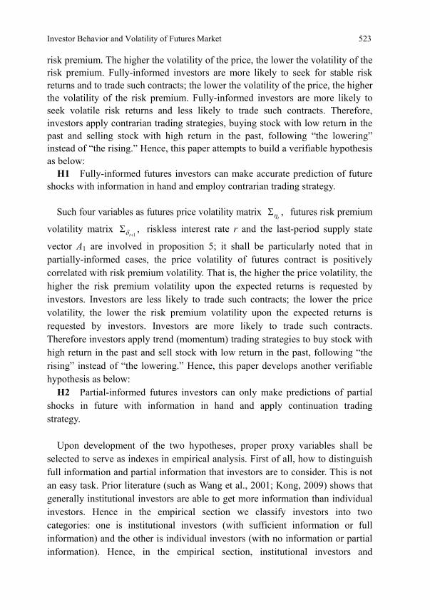
The above two tables report the statistical characteristics of investment volume and return for the two kinds of investors in Group 1 and Group 3, wherein return is the mean of the series, and the null hypothesis of T test is zero return. The two situations of “net buy-in” and “net sell-out” were distinguished. The tables show that in the net buy-in portfolio of Group 1, the return showed an increasing tendency while in the net sell-out portfolio it showed a decreasing tendency, indicating that this group of traders adopts the momentum trading strategy. In the portfolios of Group 3, the return showed a decreasing tendency for net buy-in portfolios and an increasing tendency in net sell-out portfolios, indicating that this group of traders adopts the contrarian trading strategy. Nevertheless the tendency was not obvious in 5-d and 10-d portfolios, due to short-term market

Ta

ble

2 I

nves

tmen

t Am

ount

and

Ret

urn

of “

Net

Buy

-In”

and

“N

et S

ell-O

ut”

Portf

olio

s of G

roup

1

Gro

upin

g O

bjec

tive

Portf

olio

5d

10

d 15

d 20

d 25

d 30

d 60

d

Net

buy

Av

erag

e re

turn

1.

26%

2.

52%

3.

78%

5.

04%

4.

23%

7.

56%

15

.12%

R

etur

n m

edia

n 1.

51%

2.

14%

2.

53%

5.

21%

7.

75%

13

.07%

22

.64%

T

test

(–

2.04

) (1

.74)

(1

.99)

(1

.21)

(2

.80)

(2

.26)

(2

.01)

Av

erag

e in

vest

54

550

739

10

9 00

0 00

016

4 00

0 00

021

8 00

0 00

029

8 00

0 00

032

7 00

0 00

065

5 00

0 00

0

T

test

(

1.97

)

(16.

86)

(18.

32)

(15.

56)

(14.

62)

(12.

16)

(9.2

5)

Net

sell

Aver

age

retu

rn

–3.2

3%

–6.3

2%

–11.

31%

–1

2.64

%

–14.

93%

–2

2.61

%

–45.

22%

R

etur

n m

edia

n –1

.90%

–3

.12%

–6

.86%

–6

.88%

–8

.74%

–2

2.55

%

–43.

55%

T

test

(

–4.8

5)

(–4.

05)

(–4.

017)

(–

3.15

) (–

3.28

) (–

3.06

) (–

2.57

)

Av

erag

e in

vest

–5

8 17

6 82

9–1

14 0

00 0

00–1

87 0

00 0

00–2

28 0

00 0

00–2

84 0

00 0

00–3

74 0

00 0

00–7

47 0

00 0

00

T

test

(

–2.1

4)

(–11

.37)

(–

12.9

4)

(–10

.57)

(–

15.8

3)

(–12

.37)

(–

11.6

1)

Ta

ble

3 I

nves

tmen

t Am

ount

and

Ret

urn

of “

Net

Buy

-In”

and

“N

et S

ell-O

ut”

Portf

olio

s of G

roup

3

G

roup

ing

Obj

ectiv

e

Portf

olio

5d

10d

15d

20d

25d

30d

60d

Net

buy

Aver

age

retu

rn

1.76

%

3.51

%

5.29

%

7.02

%

11.5

2%

13.0

2%

23.4

4%

R

etur

n m

edia

n 1.

85%

3.

49%

6.

12%

7.

77%

9.

48%

11

.04%

21

.40%

T

test

(3

.25)

(2

.58)

(2

.77)

(2

.36)

(5

.01)

(4

.37)

(2

.88)

Av

erag

e in

vest

1

670

000

000

3 38

0 00

0 00

05

020

000

000

6 75

0 00

0 00

08

460

000

000

10 0

00 0

00 0

0018

000

000

000

T

test

(8

.58)

(8

.12)

(8

.6)

(7.7

1)

(8.0

7)

(8.0

9)

(8.4

3)

Net

sell

Aver

age

retu

rn

–5.5

9%

–10.

89%

–1

6.76

%

–21.

78%

–3

1.91

%

–31.

12%

–5

4.46

%

R

etur

n m

edia

n –5

.46%

–9

.12%

–1

4.80

%

–22.

44%

–3

0.66

%

–32.

66%

–5

8.51

%

T

test

(–

6.98

) (–

6.09

) (–

6.08

) (–

6.45

) (–

3.84

) (–

6.42

) (–

6.71

)

Av

erag

e in

vest

–1

140

000

000

–2 2

30 0

00 0

00–3

430

000

000

–4 4

50 0

00 0

00–6

280

000

000

–6 3

60 0

00 0

00–1

1 10

0 00

0 00

0

T te

st

(–12

.34)

(–

10.6

1)

(–9.

03)

(–8.

93)

(–6.

91)

(–8.

02)

(–3.

87)

Not

e: in

vest

men

t uni

t is h

and

(one

han

d cu

prum

= 5

tons

). In

the

form

, mos

t T te

st re

sults

are

sign

ifica

nt.


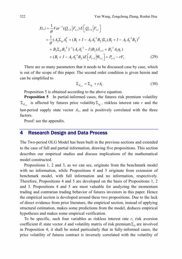
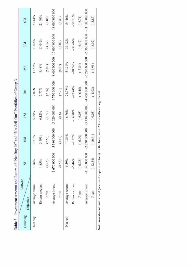
volatility. In 60-d portfolios, however, this tendency was obvious, which is illustrated in Fig. 2.

Fig. 2 60-d Momentum Effect and Contrarian Effect of Two Investor Groups

Fig. 2 shows that investors of Group 1 adopted net buy-in strategy in the rising channel of return and net sell-out strategy in the descending channel of return, which is a typical momentum trading mode; and that investors of Group 3 adopted net buy-in strategy in the descending channel of return and net sell-out strategy in the rising channel of return, which is a typical contrarian trading mode. Thus both H1 and H2 were supported.

After the momentum and contrarian trading modes of futures investors were proved by constructing “net buy-in” and “net sell-out” portfolios, we conduct additional tests to check the robustness of the results. Without distinguishing between “net buy-in” and “net sell-out”, we built 5-day, 10-day, 15-day, 20-day, 25-day, 30-day, 60-day and 90-day portfolios for the two investor groups, 16 types of portfolios in total and sum up within each portfolio. The correlogram and Q statistic test show that the 5d and 10d portfolios of Group 1 are second-order serial correlated, that the 5d portfolios of Group 3 are first-order serial correlated, that the 10d portfolios are second-order serial correlated ; and that the other portfolios are not serial correlated. For portfolios which are first-order serial correlated, AR (1) model was adopted to calibrate the standard error series. AR (2) model was adopted to calibrate the standard error series for those portfolios which are second-order serial correlated. The empirical results of investment amount and return of the two investor groups were presented in Table 4 after t value adjustment.

Ta

ble

4 I

nves

tmen

t Am

ount

and

Ret

urn

of In

vest

or G

roup

s with

out D

istin

guis

hing

bet

wee

n N

et B

uy-I

n an

d N

et S

ell-O

ut

G

roup

ing

Obj

ectiv

e

Portf

olio

5d

10d

15d

20d

25d

30d

60d

90d

Gro

up 1

Ret

urn

Rat

e –1

.01%

–2

.03%

–3

.04%

–4

.06%

–4

.93%

–6

.09%

–1

2.17

%

–18.

36%

M

edia

n –0

.005

65

–1.7

0%

–2.0

2%

–2.8

3%

–3.3

9%

4.60

%

–5.2

0%

2.02

%

T

test

(3

.06)

(2

.24)

(–

1.97

) (2

.57)

(–

2.49

) (–

2.31

) (–

2.15

) (2

.93)

In

vest

am

ount

–9

03 3

74.6

–1 8

06 7

49

–2 7

10 1

24–3

613

498

–2 0

60 0

78–5

420

248

–10

840

495

–2 1

13 2

72

T

test

(–

1.97

) (–

2.22

) (–

2.32

) (–

2.26

) (–

2.11

) (–

2.26

) (–

2.27

) (–

2.04

)

Gro

up 3

Ret

urn

Rat

e –0

.83%

–1

.64%

–2

.47%

–3

.29%

–3

.95%

–4

.93%

–9

.86%

–1

4.66

%

M

edia

n –0

.005

5

–1.5

0%

–2.0

2%

–2.8

3%

–3.3

9%

–4.6

0%

–5.2

0%

2.02

%

T

test

(3

.04)

(1

.63)

(–

2.36

) (–

2.48

) (–

2.39

) (–

2.53

) (–

2.05

) (–

2.91

)

In

vest

am

ount

48

7 00

0 00

097

4 00

0 00

0 1

460

000

000

1 95

0 00

0 00

02

470

000

000

2 92

0 00

0 00

05

840

000

000

8 95

0 00

0 00

0

T

test

(–

0.10

) (3

.88)

(3

.91)

(3

.82)

(4

.70)

(3

.67)

(4

.60)

(6

.40)


The return variance curves for 90d portfolios are in Fig. 3.

Fig. 3 Momentum and Contrarian Effects of Investor Groups without Distinguishing Net Buy-In and Net Sell-Out

The above figures show that, during the process of continuing decrease of

return, the investors of Group 1 adopted trading strategies of buy-sell-buy- sell-sell, which is the typical momentum mode; while the investors of Group 3 were buying continuously, which is the typical contrarian trading mode. Thus H1 and 2 were supported. The results of robustness check also confirmed the main findings. The empirical section of this paper showed that H1 and 2 are supported, namely, that partial-informed investors usually adopt momentum trading strategy while well-informed investors usually adopt contrarian trading mode; moreover, the longer the cycle is, the more significant momentum and contrarian effects are. And this conclusion is obviously different from prior literature on the investor behavior which argues that there is no momentum effect in Chinese stock market.

6 Conclusion

To sum up, based on a view of behavioral finance research that investors have momentum trading strategy and contrarian trading strategy, this study introduced a two-period OLG model into the futures market and developed an investor behavior model based on futures market. Moreover, the model was also extended to two situations with complete and incomplete information. We then examined futures market’s volatility by equilibrium analysis and solved first-order and second-order conditions. The results indicate that the price volatility of futures contract is affected by riskless interest rate of bonds, investors’ risk aversion coefficient, contract supply state and risk premium volatility, which is summed up by the five propositions herein.

After construction of the mathematic model, this paper further deduced two hypotheses on the basis of the five propositions. Using cuprum tick data in SHFE, we test the two hypotheses. Results partially supported the theoretical model and found that in the Chinese futures market, well-informed investors (e.g.,


institutional investors) usually adopt contrarian trading strategy, whereas partial-informed investors (e.g., individual investors) usually adopt momentum trading strategy. Hence there are obvious differences between Chinese futures market and stock market. More in-depth research on trading modes of heterogeneous investors in the Chinese futures market is likely to assist investors’ decision-making and related market supervision.

Acknowledgements This work is supported by the National Natural Science Foundation of China (70873055), the Humanities and Social Science Research Projects of the Ministry of Education of China (08JA790064), and National 985 Project of Non-traditional Security at Huazhong University of Science and Technology.

References

Barberis, N., Huang, M., & Santos, T. 2001. Prospect theory and asset prices. Quarterly Journal of Economics, 116(2): 1–63.

Barberis, N., Shleifer, A., & Vishny, R. 1998. A model of investor sentiment. Journal of Financial Economics, 49(1): 307–343.

Campell, J. 1993. Noise trading and stock price behavior. Review of Economic Studies, 60(2): 1–34.

Chan, K., Narasimhan, J., & Josef, L.1996. Momentum Strategies. The Journal of Finance, 51(3): 1681–1713.

Chen, R. 陈蓉, & Zheng, Z. 郑振龙. 2008. 期货价格能否预测未来的现货价格 (Can futures price indicate the spot price?) 国际金融研究 (Journal of International Financial Studies), 30(9): 70–74.

Chen, R. 陈蓉, & Zheng, Z. 郑振龙. 2009. 结构突变、推定预期与风险溢酬 (Structural changes, presumptive expectations and risk premium). 世界经济 (World Economy), 28(6): 64–76.

Daniel, K., Hirshleifer, D., & Subrahmanyam, A. 1998. Investor psychology and security market under-and overreactions. The Journal of Finance, 45(6): 1839–1868.

De Long, J. B., Shleifer, A., Summers, L., & Waldmann, R. 1989. The size and incidence of the losses from noise trading. Journal of Finance, 44(1): 681–696.

De Long, J. B., Shleifer, A., Summers, L., & Waldmann, R. 1990a. Noise trading risk in financial markets. Journal of Political Economy, 98(5): 703–738.

De Long, J. B., Shleifer, A., Summers, L., & Waldmann, R. 1990b. Positive feedback investment strategies and destabilizing rational speculation. Journal of Finance, 45(2): 375–395.

Deng, M. 2006. The investor behavior and stock price behavior. Journal of Banking and Finance, 36(6): 1–31.

Dumas, B., Kurshev, A., & Uppal, R. 2005. What can rational investors do about excessive volatility and sentiment fluctuations? Swiss Finance Institute Research Paper Series, 1–45.

Engle, C. 1996. The forward discount anomaly and the risk premium: A survey of recent evidence. Journal of Empirical Finance, 24(3): 123–192.


Hokkio, C., & Rush, M.1989. Market efficiency and cointegration: An application to the sterling and deutschemark exchange markets. Journal of International Money and Finance, 32(8): 75–88.

Hua, R. 华仁海, & Zhong, W. 钟伟俊. 2002. 对我国期货市场量价关系的实证分析 (The empirical analysis of relation of quantity and price in China’s forward market). 数量经济与

技术经济研究 (The Journal of Quantitative & Technical Economics), 15(6): 119–121. Jegadeesh, N., & Titman, S. 1993. Returns to buying winners and selling losers: Implications

for stock market efficiency. Journal of Finance, 48(1): 65–91. Kong, D. 孔东民. 2009. 信念、交易行为与资产价格波动：理论与实证 (Belief, trading

behavior and asset volatility: theory and empirical studies). 金融学季刊 (Quarterly Journal of Finance), 3(1): 1–28.

Leuthold, R. M. 1974. The price performance on the futures markets of a nonstorable commodity. American Journal of Agricultural Economics, 56(1): 271–290.

Martin, L., & Garcia, P. 1981. The Price-forecasting performance of futures markets for live cattle and hogs: A disaggregated analysis. American Journal of Agricultural Economics, 51(2): 63–84.

Shiller, R. S. 1981. The use of volatility measures in assessing market efficiency. Journal of Finance, 36(2): 291–304.

Spiegel, M. 1998. Stock price volatility in a multiple security overlapping generations model. Review of Financial Studies, 11(2): 419–447.

Szyszka, A. 2008. Generalized behavioral asset pricing model. Working paper, Poznan University of Economics.

Wang, C. Y. 2003. The behavior and performance of major types of futures traders. The Journal of Futures Markets, 23(1): 1–31.

Wang, J. 1993. A model of intertemporal asset prices under asymmetric information. Review of Economic Studies, 60(3): 249–282.

Wang, J. 1994. A model of competitive stock trading volume. Journal of Political Economy, 102(1): 127–168.

Wang, Y. 王永宏, & Zhao, X. 赵学军. 2001. 中国股市“惯性策略”和“反转策略”的实

证分析 (Empirical analysis on momentum strategies and contrarian strategies in Chinese stock market). 经济研究 (Economic Research Journal), (6): 56–89.

Watanabe, M. 2008. Price volatility and investor behavior in an overlapping generation model with information asymmetry. The Journal of Finance, 63(1): 229–272.

Appendix

Proposition 1 Demand of futures contract is affected by risk premium and its price, and it is positively correlated with the risk premium and negatively correlated with the price.

Proof: from Equation (11),

1t

t

XrB

P∂

= −∂

, t

t

Xr

F∂

= −∂

, known 0,r >


hence tX is positively correlated with tP and negatively correlated with .tF . This completes the proof.

Proposition 2 Futures contract state vector A is symmetric and can be expressed as:

11 12 2 2

1 2 2 21 1 1 .2 4

r r rArη η η δ ηθ θ

− −− −⎡ ⎤+⎛ ⎞ ⎛ ⎞= − Σ + Σ − Σ Σ Σ⎢ ⎥⎜ ⎟ ⎜ ⎟

⎝ ⎠ ⎝ ⎠⎢ ⎥⎣ ⎦ (A1)

The futures price volatility can exist even in the absence of risk premium. Proof: starting from Equation (16), since ηΣ and δΣ is symmetric,

variance-covariance matrix, the first item and the third item in Equation (16) are symmetric. In addition, r and θ are scalars, so A is surely a symmetric vector. Therefore, A can be substituted by TA , the transpose of A. With substitution

method, given 1 12 2Y Aη η= Σ Σ , multiply

12ηΣ on the left and the right side of

Equation (16) respectively:

1 12

2 2 21 0.r rY Yr η δ ηθ+⎛ ⎞+ + Σ Σ Σ =⎜ ⎟

⎝ ⎠ (A2)

Equation (18) is a quadratic matrix. Plus 21

4r Iθ⎛ ⎞⎜ ⎟⎝ ⎠

on both sides of the

equation to eliminate Y and simplify, attaining:

1 12 2 22 210.5 0.25 .r r rY I I

r η δ ηθ θ+⎛ ⎞ ⎛ ⎞ ⎛ ⎞+ = − Σ Σ Σ⎜ ⎟ ⎜ ⎟ ⎜ ⎟

⎝ ⎠ ⎝ ⎠ ⎝ ⎠ (A3)

Extract the root, then:

11 12 2 22 21 1 1 .

2 4r r rY I I

r η δ ηθ θ

⎛ ⎞+⎛ ⎞ ⎛ ⎞= − + − Σ Σ Σ⎜ ⎟⎜ ⎟ ⎜ ⎟⎜ ⎟⎝ ⎠ ⎝ ⎠⎝ ⎠ (A4)

Taking 1 12 2Y Aη η= Σ Σ in, Equation (16) is obtained.

For Equation (16), it may be found that δΣ doesn’t always multiply ηΣ on the right or left, and hence the futures price volatility can exist even in the absence of risk premium. This completes the proof.

Proposition 3 The price volatility of futures contract is affected by riskless interest rate r, risk aversion coefficient θ, state vector A and volatility matrix of risk premium δΣ , and follows the following equation:


2

1 11( ) ( ) .T Tr rA Arη δθ

− −+⎛ ⎞Σ = − − Σ⎜ ⎟⎝ ⎠

(A5)

The four variables have rather complicated nonlinear relation. Proof: It is already known in the previous proofs that the volatility level of

futures contract price is determined by the price covariance matrix ηΣ . Then applying reasonable transformation on Equation (16) leads to:

2

1 11( ) ( ) .T Tr rA Arη δθ

− −+⎛ ⎞Σ = − − Σ⎜ ⎟⎝ ⎠

(A6)

It can be found from the above equation that ηΣ is jointly determined by the

four variables of r, θ , TA and δΣ . Differentiating the four variables leads to the following:

12 ( )Tr Aη

θ θ−∂Σ

=∂

,

1 2 11 ( ) (2 2 ) ( )T TA r r Arη

δθ− − −∂Σ

= − − − Σ∂

,

2 2

1 21 1( ) , ( ) .T TT

r r rA Ar rA

η ηδ

δ θ− −

⎛ ⎞∂Σ ∂Σ+ +⎛ ⎞ ⎛ ⎞= − = + Σ⎜ ⎟⎜ ⎟ ⎜ ⎟⎜ ⎟∂Σ ∂⎝ ⎠ ⎝ ⎠⎝ ⎠

Therefore, level of price volatility is in complicated nonlinear relation with the four variables mentioned above. This completes the proof.

Proposition 4 In fully-informed cases, the price volatility of furtures contract is affected by riskless interest rate r, risk aversion coefficient θ, state vector A and volatility matrix of risk premium δΣ . Its vector matrix follows the following equation:

1 1 12

1 .r A A Arη δθ

− − −Σ = − − Σ (A7)

Proof: From Equation (29),

21 0.rA A Arη δθ

Σ + + Σ =

Transpose and multiply A on the right and the left side,

1 1 12

1 .r A A Arη δθ

− − −Σ = − − Σ


Therefore, the level of futures contract price volatility is determined by the four above-mentioned variables. This completes the proof.

Proposition 5 In partial-informed cases, the futures risk premium volatility

1tδ +Σ is affected by futures price volatility ,

tηΣ riskless interest rate r and the

last-period supply coefficient A1, and is positively correlated with the three. Proof: From Equation (34) one may know that

1tδ +Σ depends on

tηΣ , r and

1A , and

1 1

11 0, 0.t t

t

rA

δ δ

η

+ +∂Σ ∂Σ

= > = >∂Σ ∂

Therefore, the volatility of futures risk premium 1tδ +

Σ is positively correlated with

tηΣ and A1. This completes the proof.

Documents

Investor Behavior and Volatility of Futures Market: A