INVITED SURVEY PAPER Evolution Trends of Wireless MIMO

IEICE TRANS. COMMUN., VOL.E92–B, NO.9 SEPTEMBER 20092773

INVITED SURVEY PAPER

Evolution Trends of Wireless MIMO Channel Modeling towardsIMT-Advanced

Chia-Chin CHONG†a), Fujio WATANABE†, Nonmembers, Koshiro KITAO††, Tetsuro IMAI††,and Hiroshi INAMURA†, Members

SUMMARY This paper describes an evolution and standardizationtrends of the wireless channel modeling activities towards IMT-Advanced.After a background survey on various channel modeling approaches is in-troduced, two well-known multiple-input-multiple-output (MIMO) chan-nel models for cellular systems, namely, the 3GPP/3GPP2 Spatial ChannelModel (SCM) and the IMT-Advanced MIMO Channel Model (IMT-AdvMCM) are compared, and their main similarities are pointed out. The per-formance of MIMO systems is greatly influenced by the spatial-temporalcorrelation properties of the underlying MIMO channels. Here, we inves-tigate the spatial-temporal correlation characteristics of the 3GPP/3GPP2SCM and the IMT-Adv MCM in term of their spatial multiplexing and spa-tial diversity gains. The main goals of this paper are to summarize the cur-rent state of the art, as well as to point out the gaps in the wireless channelmodeling works, and thus hopefully to stimulate research in these areas.key words: channel model, IMT-Advanced, MIMO, multipath, spatial di-versity, spatial multiplexing

1. Introduction

Accurate knowledge of the wireless propagation channel isof great importance when designing radio systems. A real-istic radio channel model that provides insight into the radiowave propagation mechanisms is essential for the design andsuccessful deployment of wireless systems. Unfortunately,the mechanisms that govern radio propagation in a wirelesscommunication channel are complex and diverse. There-fore, a better understanding of the propagation mechanismsis key towards the development of a realistic channel model.Consequently, channel modeling has been a subject of in-tense research for a long time [1]–[5].

Standard channel models are essential for the develop-ment of new radio systems and technology. These mod-els if implemented as channel simulators allow the per-formance evaluation of different transmission technologies,signal processing techniques and receiver (RX) algorithmsthrough computer simulations. Therefore, this can avoid thenecessity to build hardware prototype or to perform field-trials for every configuration to be considered. Generallyspeaking, if accurate channel models are available, it is pos-sible to design transmission technologies and RX algorithms

Manuscript received September 8, 2008.Manuscript revised January 27, 2009.†The authors are with the Wireless Access Laboratory, DO-

COMO Communications Laboratories USA, Inc., USA.††The authors are with the Radio Access Network Develop-

ment Department, NTT DOCOMO, Inc., Yokosuka-shi, 239-8536Japan.

a) E-mail: [email protected]: 10.1587/transcom.E92.B.2773

that can achieve good performance by exploiting the prop-erties of the propagation channel. While the channel mod-els should be accurate enough in order to capture sufficientproperties from the real propagation effect, these modelsshould also be simple enough to allow feasible implemen-tation and reasonable short simulation times. Therefore,a tradeoff between “accuracy” and “simplicity” should betaken into consideration when developing a good channelmodel depending on the type of system to be evaluated.

The type of channel model that is desired depends crit-ically on the carrier frequency, bandwidth, the type of en-vironment and system under consideration. For example,different types of channel models are needed for indoorand outdoor environments, and for narrowband, widebandand ultrawideband systems. Early channel modeling workaimed to develop models which could provide an accurateestimate of the mean received power and to study the be-havior of the received signal envelope. This lead to pathlossmodels such as the Okumura-Hata model [6], Lee’s model[7], COST∗ 231 Walfish-Ikegami model [8]–[10] and theconventional statistical models for the fading signal enve-lope [2], [4], [5]. Since these models were typically devel-oped for narrowband systems, the temporal domain such asdelay spread for the power delay profile (PDP) was largelyneglected. As the need for higher data rates increased, largerbandwidths became necessary. In order to accurately modelwideband systems, narrowband channel models were en-hanced to include the prediction of the temporal domainproperties such as the delay spread of the PDP. The COST207 model [11], which was used in the evaluation of theGlobal System for Mobile Communication (GSM) systems,as well as the ITU-R∗∗ IMT-2000∗∗∗ model [12] are exam-ples of such wideband channel models. Due to the evolutionof analog to digital wideband systems, these models wereimportant when analyzing digital modulation over wirelesscommunication links and for cell planning in digital mobileradio for second generation (2G) systems.

In the third generation (3G) and Beyond 3G(B3G)/fourth generation (4G) cellular systems, higher datarate transmissions and better quality of services are de-manded in order to improve user experience. This moti-vates the investigation of how efficiently the available ra-

∗Cooperation in Science and Technology.∗∗International Telecommunications Union Radiocommunica-

tion Sector.∗∗∗International Mobile Telecommunications-2000.

Copyright c© 2009 The Institute of Electronics, Information and Communication Engineers

2774IEICE TRANS. COMMUN., VOL.E92–B, NO.9 SEPTEMBER 2009

dio channel resources should be utilized in order to fullyexploit the time, frequency, and spatial domains. Smartantennas exploit the spatial behavior of the mobile radiochannel and have been one of the key technologies to-wards the successful introduction of 3G systems such asUniversal Mobile Telecommunication System (UMTS) andCDMA2000. In order to exploit the spatial dimension ef-ficiently, it is essential to have a profound knowledge ofthe spatial-temporal propagation characteristics between abase station (BS) and a mobile station (MS). However, inmost initial 3G systems such as Wideband Code DivisionMultiple Access (WCDMA) Rel-99, High-Speed DownlinkPacket Access (HSDPA), High-Speed Uplink Packet Access(HSUPA), CDMA2000 HRPD† Rel-0, HRPD Rev-A andHRPD Rev-B, smart antennas were mainly deployed at theBS only. Therefore, at that time, most spatial channel mod-els available in the open literature only incorporated direc-tional information at the BS side [13]–[17].

The B3G and 4G cellular systems such as EvolvedHigh-Speed Packet Access (HSPA+), Long Term Evolution(LTE), LTE-Advanced, Ultra Mobile Broadband (UMB)(a.k.a. HRPD Rev-C), and Mobile WiMAX (e.g., IEEE802.16e, IEEE 802.16 m) all exploit spatial information atboth BS and MS. These systems deploy multiple-input-multiple-output (MIMO) technology whereby multiple an-tenna elements are being used at both ends of the transmis-sion link. MIMO has emerged as one of the most promisingbreakthroughs in wireless communications due to its capa-bility of improving link reliability and to significantly in-crease the link capacity [18]–[21] as long as the channelprovides sufficient scattering. Such advantages can enhancethe network’s quality of service and increase the operator’srevenues due to higher spectral efficiency and throughput.However, the actual performance of the MIMO systems isvery much influenced by the wireless channel under con-sideration. For instance, the degree of spatial correlationamong the antenna elements, the local scattering angularspread, the rank of the MIMO channel, etc. are some of theimportant limiting factors for the achievable capacity anddiversity gains. Therefore, appropriate characterization andmodeling of MIMO propagation channels are essential fordesigning MIMO transceiver and evaluating MIMO perfor-mance.

The concept of the double-directional channel was firstintroduced in [22] and since then, many channel measure-ment and modeling works based on this concept were re-ported in the literature [23]–[31]. Such a model is usefulfor MIMO systems since it includes angular information atboth the BS and the MS, and it is more well-known amongthe industrials as simply MIMO channel. The standardiza-tion of MIMO channel models were reported in 3GPP and3GPP2 (i.e., 3GPP/3GPP2 Spatial Channel Model (SCM)[32]), WiMAX Forum (i.e., Mobile WiMAX MIMO Chan-nel Model [33]), IEEE 802.11n (i.e., TGn Channel Mod-els [34]), and ITU-R Working Party 5D (WP5D) (i.e., IMT-Advanced MIMO Channel Model (IMT-Adv MCM) [35])for cellular, mobile broadband wireless access, wireless lo-

cal area networks (WLANs) and IMT-Advanced systems,respectively. The main focus of this paper are the standard-ized MIMO channel models used in both 3G and B3G/4Gcellular systems, namely, the 3GPP/3GPP2 SCM and theIMT-Adv MCM. Other standardized models designed forsingle-input-multiple-output (SIMO) or single-input-single-output (SISO) channels will not be discussed here.

The paper is organized as follows. Section 2 estab-lishes the fundamental concepts and background for vari-ous channel modeling approaches; Sect. 3 discusses the twowell-known standard MIMO channel models, namely, the3GPP/3GPP2 SCM and the IMT-Adv MCM, used in 3Gand B3G/4G cellular systems; Sect. 4 compares these twoMIMO channel models in term of their spatial multiplex-ing and spatial diversity gains; finally, in Sect. 5 appropriateconclusions are drawn.

2. Channel Modeling Approach

The requirement to model many different types of wirelesspropagation channels has resulted in a large number of dif-ferent modeling approaches reported in the literature [36]–[38]. One reason for the abundance of modeling approachesis due to the complex phenomena encountered by a transmit-ted signal. The transmitted signal will usually arrive at theRX via several paths, i.e., multipaths, where the signal en-counters various propagation mechanisms such as reflection,scattering and/or diffraction. Figure 1 illustrates a typicalwireless channel in outdoor environment whereby, a signaltransmitted by the BS is reflected by several objects withinthe channel before reaching the MS. Therefore, many dif-ferent types of simplifications and approximations are nec-essary in order to obtain a simple yet accurate and reliablemodel of the wireless communications channel. Accordingto [39], propagation channel models can be broadly dividedinto two main categories, namely, deterministic approachand stochastic approach (or statistical approach). In gen-eral, these models differ in terms of their usage and the typeof underlying data. Under each category, channel modelscan be further grouped according to the method by whichthey were developed as summarized in Fig. 2. In this sec-tion, some existing channel models in each category are re-ferred. The list is not meant to be exhaustive, but merelyserve as a stepping-stone towards the discussion in the restof the paper.

2.1 Deterministic Approach

There are three different subcategories of deterministic ap-proach, namely, closed-form approach, measurement-basedapproach and ray-tracing approach. Deterministic modelsmay exist in closed-form for very simple channels such as atwo-path signal model. Such models are usually too restric-tive to represent any realistic communication environment.Direct measurement of the channel impulse response pro-vides an empirical model for the measured scenarios. The

†High Rate Packet Data.

CHONG et al.: EVOLUTION TRENDS OF WIRELESS MIMO CHANNEL MODELING TOWARDS IMT-ADVANCED2775

Fig. 1 Illustration of a typical wireless channel in outdoor environment.

Fig. 2 Classification of channel modeling approaches.

data is usually collected with channel sounders by transmit-ting known signals and comparing them with the receivedsignals. The main advantage of such an approach is thatthe measured channel responses are usually very accurate.However, the downside is that the measured data is very site-specific and therefore, characterization of all types of chan-nels by measurement becomes a non-trivial task due to therequirement of vast amount of data. Furthermore, channelmeasurements are very costly, which limits the amount ofdata that can be collected. A number of measurement-baseddeterministic channel models have been developed and re-ported in the literature [40], [41].

Ray-tracing approach apply an electromagnetic simu-lation tool such as ray launching and imaging methods toobtain nearly exact propagation characteristics for a spec-ified geometry. Firstly, a site-specific environment is gen-erated from a detailed map, in which the BSs and MSs areplaced. Then, based on the known transmitting signals thesemodels describe the physics of the propagation mechanisms(e.g., reflection, diffraction and scattering) in order to cal-culate the received signals. Note that, these calculations re-quire a far-field assumption to be feasible. The accuracyof the models rely on the accuracy and detail of the site-specific propagation medium [42]. Therefore, this approachshould be employed only when detailed environment data isavailable such as the position, size and orientation of man-

made objects (e.g., buildings, bridges, roads, etc.) as wellas natural objects (e.g., trees, mountains, etc.). The basicidea behind the ray-tracing approach is that, if the propaga-tion environment is known to a sufficient degree, wirelesspropagation is a deterministic process that allows determin-ing its characteristics at every point in space. Typically, theray-tracing approach is used for cell and network planning.The major advantage of ray-tracing models is that they of-fer great accuracy with site-specific results. Ideally, any sitecan be modeled if its physical characteristics are available,and any channel parameter can be calculated by adjustingthese models. However, in reality these physical parame-ters are either unavailable or cannot be perfectly obtained.This subsequently could lead to degradation in the accuracyof the ray-tracing model. Furthermore, these models haveseveral disadvantages. Firstly, the topographical and envi-ronment data is always tied to a particular site and thus,a huge amount of such data is required in order to obtaina comprehensive set of different propagation environments.Secondly, they are usually computationally expensive, es-pecially when the environment is complex. Thus, detailedphysical characteristics of the simulated environment mustbe known beforehand which is often time-consuming andimpractical. Numerous ray-tracing models for cellular net-works have been reported in the literature such as [43]–[53]and the references therein.

2.2 Stochastic Approach

Stochastic models are normally less complex than the deter-ministic models, and can provide sufficiently accurate chan-nel information. These models attempt to generate syntheticchannel responses that are representative of real propagationchannels. Firstly, measurements will be conducted in a largevariety of locations and environments in order to obtain adatabase with good representation of the underlying statisti-cal properties. Then, the probability density function (pdf)of the channel parameters will be derived from the measure-ment data which will be used to regenerate the channel im-pulse responses. Since the stochastic approach is based onprobabilistic characterization of the wireless channel, mod-els based on this approach can be tuned to imitate variouspropagation environments by setting appropriate values forthe channel parameters. Note that fixed parameter settingsdo not produce identical outputs on each simulation run butstochastic processes are used to create variability within afixed environment type. For example, a particular set of pa-rameters might generate a representative set of propagationscenarios found in outdoor urban environments. Many chan-nel models have been developed under this category for cel-lular systems design and cell planning such as the Okumura-Hata pathloss model [6], the widely used COST 207 model[11], its successors UMTS Code Division Testbed (CODIT)model [54] and Advanced Time Division Multiple Access(ATDMA) model [55].

In general, stochastic approach can be classified intotwo main subcategories, namely, ray-based approach (a.k.a.


geometrically-based stochastic approach) and correlation-based approach. The ray-based modeling approach is com-monly used in MIMO channel modeling. This approachassumes that a number of scatterers is distributed in spaceaccording to some stochastic distribution around the trans-mitter (TX) and RX ends. The channel gains are thencalculated for each antenna at both TX and RX ends bysumming the contribution from each reflected ray emergingfrom the scatterer. Multiple rays, each with its own am-plitude, angle-of-departure (AoD), angle-of-arrival (AoA),time-of-arrival (ToA), and phase, add constructively and de-structively, whereby the received signal can be modeled as asuperposition of rays. The summed received signal can thenbe written as

h(t) =N∑

n=1

αnexp ( j2π fnt + φn), (1)

where αn is the amplitude, fn is the frequency, and φn is thephase of the n-th ray. Within this subcategory, the widelydeployed models are the 3GPP/3GPP2 SCM [32] and theIMT-Adv MCM [35] for 3G and B3G/4G cellular systems,respectively. Other examples of ray-based models are suchas [56]–[61].

The correlation-based modeling approach relies on thechannel second order statistics such as correlation and co-variance matrices. In particular, this approach models thetransfer function of each transmit and receive antenna ele-ment pair, and the signal correlations between them. Thegeneration of MIMO channel matrices based on channelcorrelation matrix is defined as

R = E[vec (H)H vec (H)

], (2)

where E[·] denotes the expectation, (·)H denotes the Hermi-tian transpose, vec(·) is the vectorization operator, and H isthe MIMO channel matrix. In order to simplify the analy-sis, one example of such a model is the Kronecker modelin which the channel correlation matrix R can be written asfollows

R = RTx ⊗ RRx, (3)

where ⊗ is the Kronecker product and RTx and RRx are thecorrelation matrices at the TX and RX, respectively. Theadvantage of the Kronecker assumption is that (3) is a com-putationally simpler operation than the full correlation ma-trix in (2). The underlying assumption is that the directionalproperties of the channel at the TX and RX are independent.

Both ray-based and correlation-based stochastic chan-nel models have advantages and disadvantages. For in-stance, the ray-based channel models can directly generatechannel coefficients, in which the spatial-temporal correla-tion is implicitly present in the channel matrix generation.However, since it does not specify the spatial-temporal cor-relation properties explicitly, it is therefore difficult to con-nect its simulation results with the theoretical analysis. Fur-thermore, the implementation complexity of the ray-based

Fig. 3 Illustration of the ray-based MIMO channel model.

Fig. 4 Illustration of the correlation-based (Kronecker approach) MIMOchannel model.

models are usually high since many parameters have to begenerated such as antenna array orientations, mobile di-rections, delay spread, angular spread, AoDs, AoAs, andphases. On the other hand, for the correlation-based mod-els, the spatial correlation is explicitly defined and gener-ated by means of spatial correlation matrices. This provideselegant and concise analytical expressions for the MIMOchannel and makes the correlation-based models easier tobe integrated into a theoretical framework. The main ad-vantage of the correlation-based approach are its compu-tational and modeling simplicity whereby it requires lessinput parameters as compared to the ray-based approach.However, despite its simplicity and analytical tractability,the correlation-based model is restricted to model only theaverage spatial-temporal behavior of the MIMO channels.There are several other drawbacks of the correlation-basedapproach. For instance, the correlation matrix is antennaarray dependent and hence has to be re-estimated for dif-ferent array geometries. Also, the model parameteriza-tion describes only the second-order statistics of the chan-nel without any physical interpretation of the propagationmedium. In particular, with the Kronecker assumption, thecorrelation-based models are deemed to over simplify theMIMO channel characteristics since they are incapable ofreproducing the “pinhole” [50] or “keyhole” [62], [63] ef-fects which results in low rank (hence low capacity) chan-nels. Due to the above reasons, the ray-based model is pre-ferred as it provides more insights of the variations of dif-ferent MIMO channel realizations. Figures 3 and 4 illus-trate the ray-based and the correlation-based (Kronecker ap-proach) MIMO channel models, respectively.

3. Standard MIMO Channel Models for 3G andB3G/4G Cellular Systems

In order to evaluate the performance of various air-interface


Fig. 5 The overview of the 3GPP/3GPP2 SCM channel coefficients generation procedure [32].

technologies based on MIMO schemes, several MIMOchannel models have been developed in either standard orga-nizations (e.g., 3GPP/3GPP2 SCM and IMT-Adv MCM) orwithin large collaborative projects (e.g., IST Multi ElementTransmit and Receive Antennas (METRA) Channel Model[25], IST Wireless World Initiative New Radio (WINNER)model [64], COST 259 Directional Channel Model [29], andCOST 273 MIMO Channel Model [65]). In this section,two MIMO channel models, i.e., the 3GPP/3GPP2 SCMand the IMT-Adv MCM suitable for system-level simula-tions will be reviewed and compared. Both models de-ploy the geometrically-based stochastic modeling approachas the channel model framework and can be applied for dif-ferent environments (e.g., urban macro, urban micro, etc.).Each environment has specific distributions and parameters.By changing these specific distributions in angle and delaydomains as well as the environment specific parameters, dif-ferent channel models under different environments and sce-narios (e.g., line-of-sight (LOS) and non-LOS (NLOS)) canbe generated.

3.1 3GPP/3GPP2 Spatial Channel Model (SCM)

The SCM was developed within 3GPP/3GPP2 ad-hoc groupas a reference model for evaluating different MIMO tech-niques. The model was first released in September 2003[66] and was later updated in June 2007 [32]. It definesthree most commonly used environments in cellular sys-tems, namely, suburban macro, urban macro, and urban mi-cro. For all these scenarios, the number of paths (a.k.a. clus-ters) are fixed to six and each path consists of 20 spatiallyseparated subpaths (a.k.a. rays). The SCM was parameter-ized for systems with 5 MHz bandwidth and a center fre-quency around 2 GHz. Therefore, it is valid for most 3G sys-

tems deploying MIMO techniques and may not be suitablefor system with bandwidth higher than 5 MHz. The SCMwas later extended by [67] as the Spatial Channel Model Ex-tension (SCME) which support up to 100 MHz bandwidth inorder to evaluate the 3GPP LTE systems.

The overall procedure for generating the SCM channelcoefficients can be summarized in three steps as illustratedin Fig. 5. Firstly, one of the three environments as describedabove will be chosen. After the number of BSs with theirrespective cell layouts (e.g., hexagonal layout) and inter-sitedistances have been determined, MSs are randomly posi-tioned within each cell. Then, each of the MS will be givena random antenna array orientation drawn from a uniform[0, 360◦] distribution and a random velocity with its direc-tion also drawn from a uniform [0, 360◦] distribution. Sec-ondly, the channel parameters for the selected environmentwill be determined. This can be categorized into large-scale(LS) parameters such as delay spread (DS), angular spread(AS) and shadowing fading (SF); and small-scale (SS) pa-rameters such as paths’ powers, delays, AoAs and AoDs,as well as subpaths’ AoAs and AoDs. Thirdly, the chan-nel coefficients are generated. Based on the SCM, six pathsare generated, each with a given angular dispersion power,AoA and AoD. This dispersion is due to the fact that thereare 20 subpaths within each path, and each subpath has aslightly different AoA and/or AoD but with the same timedelay. Here, the paths’ powers, delays, and angular proper-ties for both sides of the link are modeled as random vari-ables (RVs) defined by pdfs and cross-correlations.

When generating channel coefficients using the SCM,a number of “drops” are generated. A “drop” is defined asa simulation run for a given number of cells/sectors, BSs,and MSs over a short period of time. During a drop, thechannel undergoes fast-fading according to the motion of


Table 1 The 3GPP/3GPP2 SCM channel model parameters [32].

Channel Scenario Suburban Macro Urban Macro Urban Micro

Number of paths, N 6 6 6Number of subpaths per path, M 20 20 20Mean AS at BS E(σAS ,BS ) = 5◦ E(σAS ,BS ) = 8◦, 15◦ NLOS: E(σAS ,BS ) = 19◦AS at BS as a lognormal RV μAS = 0.69 For 8◦, μAS = 0.81 N/AσAS = 10(εAS ·x+μAS ), εAS = 0.13 εAS = 0.34where x ∼ N(0, 1) For 15◦, μAS = 1.18

εAS = 0.21rAS = σAoD/σAS 1.2 1.3 N/APer-path AS at BS (fixed) 2◦ 2◦ 5◦ (LOS and NLOS)

BS per-path AoD distribution N(0, σ2AoD), where N(0, σ2

AoD), where U(−40◦, 40◦)standard deviation σAoD = rAS · σAS σAoD = rAS · σAS

Mean AS at MS E(σAS ,MS ) = 68◦ E(σAS ,MS ) = 68◦ E(σAS ,MS ) = 68◦Per-path AS at MS (fixed) 35◦ 35◦ 35◦

MS per-path AoA distribution N(0, σ2AoA(Pr)) N(0, σ2

AoA(Pr)) N(0, σ2AoA(Pr))

DS as a lognormal RV μDS = −6.8 μDS = −6.18 N/AσDS = 10(εDS ·x+μDS ), εDS = 0.288 εDS = 0.18where x ∼ N(0, 1)Mean total RMS DS E(σDS ) = 0.17 μs E(σDS ) = 0.65 μs E(σDS ) = 0.251 μsrDS = σdelays/σDS 1.4 1.7 N/ADistribution for path delays − − U(0, 1.2 μs)Lognormal shadowing 8 dB 8 dB NLOS: 10 dBstandard deviation, σS F LOS: 4 dBPathloss model (dB), 31.5 + 35 log10(d) 34.5 + 35 log10(d) NLOS: 34.53 + 38 log10(d)d is in meters LOS: 30.18 + 26 log10(d)

the MSs and for each of these drops, parameters describingthe channel such as DS, AS, SF, AoAs, etc. are assumed tobe fixed. For each new simulation drop, these parameters arerandomly drawn according to the specified distributions thatdepend on the environment under invetigation. Furthermore,the MS position is also drawn randomly for each new drop.Since the model is antenna independent, for each simulationrun the antenna patterns, geometries and orientations canbe chosen arbitrary. Table 1 summarizes the SCM channelparameters used in each of the environments.

In addition to the 3-steps procedure as described above,the SCM offers four optional system simulation features forspecial cases (see Fig. 5).

• Polarized arrays: The cross-polarized model is in-cluded in additional to the vertical-polarized one as-sumed in the baseline model. Cross-polarized antennaarrays will most likely to be implemented on futurehandheld devices in order to guarantee the compactsize of the devices.• Far scatterer clusters: The far scatterer clusters repre-

sent bad-urban case where additional clusters are seenin the environment. These can be due to reflectionor scattering caused by mountains, high-rise buildings,etc. The far scatterers tend to increase both the delayand angular spreads of the channel which can changethe MIMO channel characteristics significantly. Notethat this feature is limited to be used in the urbanmacrocell only.• Line-of-sight (LOS): The LOS modeling is based on

the Ricean-K factor and is available for urban micro-cell only. By including the LOS path in the model, the

average delay and angular spreads are reduced, whichrepresent a highly correlated MIMO channel.• Urban canyon: Urban canyon exists in dense urban

areas where signals propagate between buildings whichtypically occur in both macrocells and over rooftop mi-crocells. Under this environment, multipath arrive atthe MS are usually from similar angles which give riseto narrow AS. Therefore, this tends to increase the cor-relation at the MS. This feature is available for urbanmacrocell and urban microcell.

Interested readers are referred to [32] and [68] formore comprehensive description and evaluation of the3GPP/3GPP2 SCM.

3.2 ITU-R IMT-Advanced MIMO Channel Model (IMT-Adv MCM)

The Drafting Group Evaluation Channel Model (DG-EVALChannel Model) was formed within the ITU-R in order todevelop standard MIMO channel modeling approach for theevaluation of IMT-Advanced candidate radio interface tech-nologies (RITs). The DG-EVAL Channel Model was es-tablished in May 2007 during the 22nd Meeting of ITU-R Working Party 8F (WP8F) in Kyoto, Japan. The workwithin the group was continued in January 2008 during the1st Meeting of ITU-R WP5D in Geneva, Switzerland andwas finalized in July 2008 during the 2nd Meeting of ITU-R WP5D in Dubai, United Arab Emirates. The IMT-AdvMCM covers all the required test environments (TEs) andscenarios as defined in the IMT-Advanced RITs EvaluationGuidelines (IMT.EVAL) [35] which can be summarized asbelow:


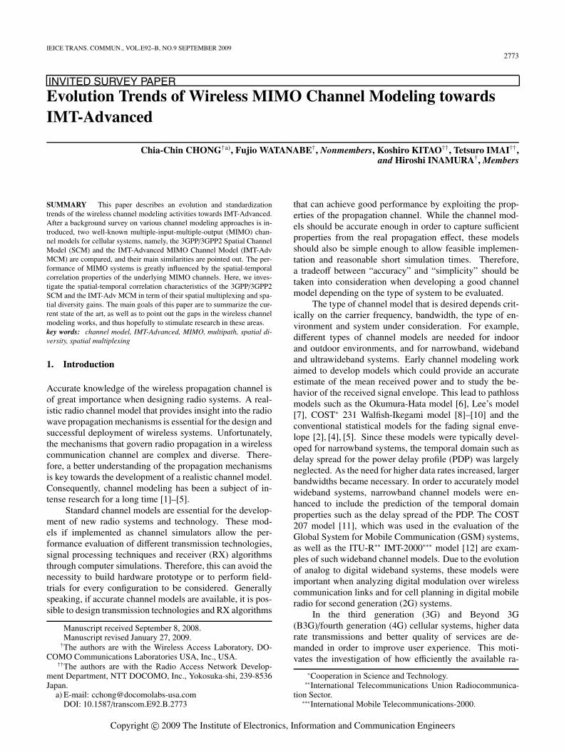
Fig. 6 The ITU-R IMT-Advanced MIMO channel model [35].

• Base Coverage Urban TE: Urban macrocell (UMa)scenario and suburban macrocell (SMa) scenario tar-geting on continuous coverage for pedestrian up to fastvehicular users. Note that SMa is defined as an optionalscenario for evaluation within the WP5D.• Microcellular TE: Urban microcell (UMi) scenario

targeting on pedestrian and slow vehicular users inhigher user density area.• Indoor TE: Indoor hotspot (InH) scenario targeting on

stationary and pedestrian in isolated cells.• High Speed TE: Rural macrocell (RMa) scenario tar-

geting on high-speed vehicular and trains.

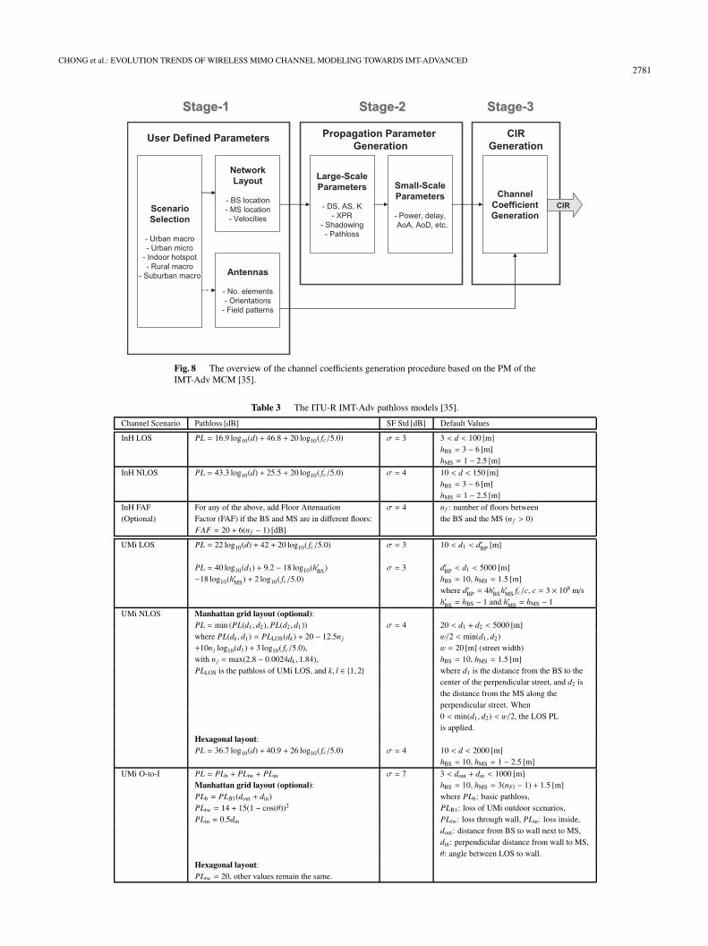
The IMT-Adv MCM consists of a Primary Module(PM) and an Extension Module (EM) as illustrated in Fig. 6.The PM defines the mandatory channel model definition andparameter tables required for evaluation of IMT-Advancedcandidate RITs in four mandatory scenarios i.e., UMa, UMi,InH and RMa. The EM is an optional feature available forUMa, RMa and SMa scenarios to cover cases beyond IMT-Advanced. In the rest of the paper, only the mandatory PMwill be discussed.

The framework of the PM is based on the WINNERII channel model [64] which was developed within the Eu-ropean collaborate research project IST-WINNER. The PMis based upon the SCM methodology and is further ex-tended to support system with larger bandwidths (i.e., up to100 MHz) and different carrier frequencies (i.e., 2–6 GHz)in larger variety of different scenarios (i.e., from outdoorto indoor). The model parameters are determined from ex-tensive wideband MIMO radio-channel measurement cam-paigns performed within IST-WINNER project and from re-sults obtained in the literature. Within the PM, two modelsare defined, namely, the generic model and the clustered de-lay line (CDL) model. The generic model which is described

Fig. 7 The elements of the MIMO channel model as defined in the PM[35].

by one mathematical framework through different parame-ter sets will be used as the mandatory system-level model,while the CDL model is a reduced variability model withfixed parameter sets will only be used for calibration pur-poses.

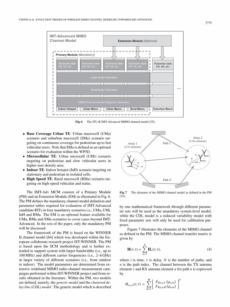
Figure 7 illustrates the elements of the MIMO channelas defined in the PM. The MIMO channel transfer matrix isgiven by

H(t; τ) =N∑

n=1

Hn(t; τ), (4)

where t is time, τ is delay, N is the number of paths, andn is the path index. The channel between the TX antennaelement s and RX antenna element u for path n is expressedby

Hu,s,n(t; τ) =M∑

m=1

[FRx,u,V

(ϕn,m)

FRx,u,H(ϕn,m)]T


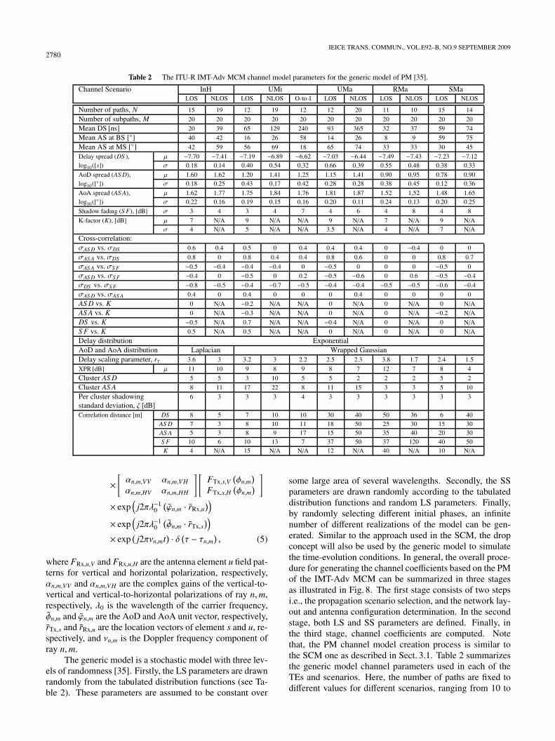
Table 2 The ITU-R IMT-Adv MCM channel model parameters for the generic model of PM [35].

Channel Scenario InH UMi UMa RMa SMaLOS NLOS LOS NLOS O-to-I LOS NLOS LOS NLOS LOS NLOS

Number of paths, N 15 19 12 19 12 12 20 11 10 15 14

Number of subpaths, M 20 20 20 20 20 20 20 20 20 20 20

Mean DS [ns] 20 39 65 129 240 93 365 32 37 59 74

Mean AS at BS [◦] 40 42 16 26 58 14 26 8 9 59 75

Mean AS at MS [◦] 42 59 56 69 18 65 74 33 33 30 45

Delay spread (DS ), μ −7.70 −7.41 −7.19 −6.89 −6.62 −7.03 −6.44 −7.49 −7.43 −7.23 −7.12log10([s]) σ 0.18 0.14 0.40 0.54 0.32 0.66 0.39 0.55 0.48 0.38 0.33

AoD spread (AS D), μ 1.60 1.62 1.20 1.41 1.25 1.15 1.41 0.90 0.95 0.78 0.90log10([◦]) σ 0.18 0.25 0.43 0.17 0.42 0.28 0.28 0.38 0.45 0.12 0.36

AoA spread (AS A), μ 1.62 1.77 1.75 1.84 1.76 1.81 1.87 1.52 1.52 1.48 1.65log10([◦]) σ 0.22 0.16 0.19 0.15 0.16 0.20 0.11 0.24 0.13 0.20 0.25

Shadow fading (S F), [dB] σ 3 4 3 4 7 4 6 4 8 4 8

K-factor (K), [dB] μ 7 N/A 9 N/A N/A 9 N/A 7 N/A 9 N/Aσ 4 N/A 5 N/A N/A 3.5 N/A 4 N/A 7 N/A

Cross-correlation:σAS D vs. σDS 0.6 0.4 0.5 0 0.4 0.4 0.4 0 −0.4 0 0

σAS A vs. σDS 0.8 0 0.8 0.4 0.4 0.8 0.6 0 0 0.8 0.7

σAS A vs. σS F −0.5 −0.4 −0.4 −0.4 0 −0.5 0 0 0 −0.5 0

σAS D vs. σS F −0.4 0 −0.5 0 0.2 −0.5 −0.6 0 0.6 −0.5 −0.4

σDS vs. σS F −0.8 −0.5 −0.4 −0.7 −0.5 −0.4 −0.4 −0.5 −0.5 −0.6 −0.4

σAS D vs. σAS A 0.4 0 0.4 0 0 0 0.4 0 0 0 0

AS D vs. K 0 N/A −0.2 N/A N/A 0 N/A 0 N/A 0 N/A

AS A vs. K 0 N/A −0.3 N/A N/A 0 N/A 0 N/A −0.2 N/A

DS vs. K −0.5 N/A 0.7 N/A N/A −0.4 N/A 0 N/A 0 N/A

S F vs. K 0.5 N/A 0.5 N/A N/A 0 N/A 0 N/A 0 N/A

Delay distribution ExponentialAoD and AoA distribution Laplacian Wrapped GaussianDelay scaling parameter, rτ 3.6 3 3.2 3 2.2 2.5 2.3 3.8 1.7 2.4 1.5

XPR [dB] μ 11 10 9 8 9 8 7 12 7 8 4

Cluster AS D 5 5 3 10 5 5 2 2 2 5 2

Cluster AS A 8 11 17 22 8 11 15 3 3 5 10

Per cluster shadowing 6 3 3 3 4 3 3 3 3 3 3standard deviation, ζ [dB]Correlation distance [m] DS 8 5 7 10 10 30 40 50 36 6 40

AS D 7 3 8 10 11 18 50 25 30 15 30AS A 5 3 8 9 17 15 50 35 40 20 30S F 10 6 10 13 7 37 50 37 120 40 50K 4 N/A 15 N/A N/A 12 N/A 40 N/A 10 N/A

×[αn,m,VV αn,m,VH

αn,m,HV αn,m,HH

] [FTx,s,V

(φn,m)

FTx,s,H(φn,m)]

× exp(

j2πλ−10(ϕn,m · rRx,u

))× exp

(j2πλ−1

0(φn,m · rTx,s

))× exp

(j2πνn,mt

) · δ (τ − τn,m), (5)

where FRx,u,V and FRx,u,H are the antenna element u field pat-terns for vertical and horizontal polarization, respectively,αn,m,VV and αn,m,VH are the complex gains of the vertical-to-vertical and vertical-to-horizontal polarizations of ray n,m,respectively, λ0 is the wavelength of the carrier frequency,φn,m and ϕn,m are the AoD and AoA unit vector, respectively,rTx,s and rRx,u are the location vectors of element s and u, re-spectively, and νn,m is the Doppler frequency component ofray n,m.

The generic model is a stochastic model with three lev-els of randomness [35]. Firstly, the LS parameters are drawnrandomly from the tabulated distribution functions (see Ta-ble 2). These parameters are assumed to be constant over

some large area of several wavelengths. Secondly, the SSparameters are drawn randomly according to the tabulateddistribution functions and random LS parameters. Finally,by randomly selecting different initial phases, an infinitenumber of different realizations of the model can be gen-erated. Similar to the approach used in the SCM, the dropconcept will also be used by the generic model to simulatethe time-evolution conditions. In general, the overall proce-dure for generating the channel coefficients based on the PMof the IMT-Adv MCM can be summarized in three stagesas illustrated in Fig. 8. The first stage consists of two stepsi.e., the propagation scenario selection, and the network lay-out and antenna configuration determination. In the secondstage, both LS and SS parameters are defined. Finally, inthe third stage, channel coefficients are computed. Notethat, the PM channel model creation process is similar tothe SCM one as described in Sect. 3.1. Table 2 summarizesthe generic model channel parameters used in each of theTEs and scenarios. Here, the number of paths are fixed todifferent values for different scenarios, ranging from 10 to


Fig. 8 The overview of the channel coefficients generation procedure based on the PM of theIMT-Adv MCM [35].

Table 3 The ITU-R IMT-Adv pathloss models [35].

Channel Scenario Pathloss [dB] SF Std [dB] Default Values

InH LOS PL = 16.9 log10(d) + 46.8 + 20 log10( fc/5.0) σ = 3 3 < d < 100 [m]hBS = 3 − 6 [m]hMS = 1 − 2.5 [m]

InH NLOS PL = 43.3 log10(d) + 25.5 + 20 log10( fc/5.0) σ = 4 10 < d < 150 [m]hBS = 3 − 6 [m]hMS = 1 − 2.5 [m]

InH FAF For any of the above, add Floor Attenuation σ = 4 nf : number of floors between(Optional) Factor (FAF) if the BS and MS are in different floors: the BS and the MS (nf > 0)

FAF = 20 + 6(nf − 1) [dB]

UMi LOS PL = 22 log10(d) + 42 + 20 log10( fc/5.0) σ = 3 10 < d1 < d′BP [m]

PL = 40 log10(d1) + 9.2 − 18 log10(h′BS) σ = 3 d′BP < d1 < 5000 [m]−18 log10(h′MS) + 2 log10( fc/5.0) hBS = 10, hMS = 1.5 [m]

where d′BP = 4h′BSh′MS fc/c, c = 3 × 108 m/sh′BS = hBS − 1 and h′MS = hMS − 1

UMi NLOS Manhattan grid layout (optional):PL = min (PL(d1, d2), PL(d2, d1)) σ = 4 20 < d1 + d2 < 5000 [m]where PL(dk , d1) = PLLOS(dk) + 20 − 12.5nj w/2 < min(d1, d2)+10nj log10(d1) + 3 log10( fc/5.0), w = 20 [m] (street width)with nj = max(2.8 − 0.0024dk , 1.84), hBS = 10, hMS = 1.5 [m]PLLOS is the pathloss of UMi LOS, and k, l ∈ {1, 2} where d1 is the distance from the BS to the

center of the perpendicular street, and d2 isthe distance from the MS along theperpendicular street. When0 < min(d1, d2) < w/2, the LOS PLis applied.

Hexagonal layout:PL = 36.7 log10(d) + 40.9 + 26 log10( fc/5.0) σ = 4 10 < d < 2000 [m]

hBS = 10, hMS = 1 − 2.5 [m]

UMi O-to-I PL = PLb + PLtw + PLin σ = 7 3 < dout + din < 1000 [m]Manhattan grid layout (optional): hBS = 10, hMS = 3(nFl − 1) + 1.5 [m]PLb = PLB1(dout + din) where PLb: basic pathloss,PLtw = 14 + 15(1 − cos(θ))2 PLB1: loss of UMi outdoor scenarios,PLin = 0.5din PLtw: loss through wall, PLin: loss inside,

dout: distance from BS to wall next to MS,din: perpendicular distance from wall to MS,θ: angle between LOS to wall.

Hexagonal layout:PLtw = 20, other values remain the same.


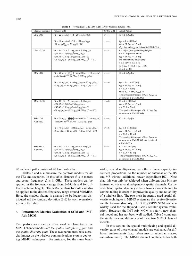
Table 4 (continued) The ITU-R IMT-Adv pathloss models [35].

Channel Scenario Pathloss [dB] SF Std [dB] Default Values

UMa LOS PL = 22 log10(d) + 42 + 20 log10( fc/5.0) σ = 4 10 < d < d′BP [m]

PL = 40 log10(d1) + 9.2 − 18 log10(h′BS) σ = 4 d′BP < d < 5000 [m]−18 log10(h′MS) + 2 log10( fc/5.0) hBS = 25, hMS = 1.5 [m]

(d′BP, hBS and h′MS are defined in UMi LOS.)

UMa NLOS PL = 101.04 − 7.1 log10(w) + 7.5 log10(h) σ = 4 h = 20 [m] (average building height)−(24.37 − 3.7(h/hBS)2) log10(hBS) w = 20 [m] (street width)+(43.42 − 3.1 log10(hBS))(log10(d) − 3) hBS = 25, hMS = 1.5 [m],+20 log10( fc) − (3.2(log10(11.75hMS))2 − 4.97) The applicability ranges: [m]

5 < h < 50, 5 < w < 50,10 < hBS < 150, 1 < hMS < 10,50 < d < 5000

RMa LOS PL = 20 log10

(4π(d)

300/ fc

)+min(0.03h1.72, 10) log10(d) σ = 4 10 < d < dBP [m]

−min(0.044h1.72, 14.77) + 0.002 log10(h)d

PL = 40 log10(d) − 20 log10(hBS) − 20 log10(hMS) σ = 6 dBP < d < 10, 000 [m]+5 log10( fc) + 11 log10(h) − 7.1 log 10(w) − 2.45 hBS = 32, hMS = 1.5 [m]

w = 20, h = 5 [m]where dBP = 2πhBShMS fc/c(The applicability ranges of h, w, hBS, hMS

are same as in UMa NLOS)

RMa NLOS PL = 101.04 − 7.1 log10(w) + 7.5 log10(h) σ = 8 50 < d < 5000 [m]−(24.37 − 3.7(h/hBS)2) log10(hBS) hBS = 32, hMS = 1.5 [m]+(43.42 − 3.1 log10(hBS))(log10(d) − 3) w = 20, h = 5 [m]+20 log10( fc) − (3.2(log10(11.75hMS))2 − 4.97) (The applicability ranges of h, W, hBS, hMS


SMa LOS PL = 20 log10

(4π(d)

300/ fc

)+min(0.03h1.72, 10) log10(d) σ = 4 30 < d < dBP [m]

(Optional) −min(0.044h1.72, 14.77) + 0.002 log10(h)d

PL = 40 log10(d) − 20 log10(hBS) − 20 log10(hMS) σ = 6 dBP < d < 5000 [m]+5 log10( fc) + 11 log10(h) − 7.1 log 10(w) − 2.45 hBS = 32, hMS = 1.5 [m]

w = 20, h = 10 [m](The applicability ranges of h, w, hBS, hMS

are same as in UMa NLOS. dBP is definedin RMa LOS.)

SMa NLOS PL = 101.04 − 7.1 log10(w) + 7.5 log10(h) σ = 8 50 < d < 5000 [m](Optional) −(24.37 − 3.7(h/hBS)2) log10(hBS) hBS = 25, hMS = 1.5 [m]

+(43.42 − 3.1 log10(hBS))(log10(d) − 3) w = 20, h = 10 [m]+20 log10( fc) − (3.2(log10(11.75hMS))2 − 4.97) (The applicability ranges of h, W, hBS, hMS


20 and each path consists of 20 fixed subpaths.Tables 3 and 4 summarize the pathloss models for all

the TEs and scenarios. In this table, distance d is in metersand center frequency fc is in GHz. These models can beapplied in the frequency range from 2–6 GHz and for dif-ferent antenna heights. The RMa pathloss formula can alsobe applied to the desired frequency range around 800 MHz.Here, the shadow fading is assumed to be lognormal dis-tributed and the standard deviation (Std) for each scenario isgiven in the table.

4. Performance Metrics Evaluation of SCM and IMT-Adv MCM

Two performance metrics often used to characterize theMIMO channel models are the spatial multiplexing gain andthe spatial diversity gain. These two parameters have a cru-cial impact on the wireless communications system deploy-ing MIMO techniques. For instance, for the same band-

width, spatial multiplexing can offer a linear capacity in-crement proportional to the number of antennas at the BSand MS without additional power expenditure [69]. Notethat, this can only be achieved when different data bits aretransmitted via several independent spatial channels. On theother hand, spatial diversity utilizes two or more antennas tocombat fading in order to improve the quality and reliabilityof a wireless link. The two most frequently used spatial di-versity techniques in MIMO system are the receive diversityand the transmit diversity. The 3GPP/3GPP2 SCM has beenwidely used for the Beyond 3G/4G cellular system evalu-ation. However, the IMT-Adv MCM is a fairly new chan-nel model and has not been well studied. Table 5 comparesthe similarities and differences of these two MIMO channelmodels.

In this section, the spatial multiplexing and spatial di-versity gains of these channel models are evaluated for dif-ferent environments (e.g., urban macro, suburban macro,and urban micro). The MIMO channel coefficients for both


Table 5 The 3GPP/3GPP2 SCM vs. ITU-R IMT-Adv MCM.

Parameters 3GPP/3GPP2 SCM IMT-Adv MCM

Environments/scenarios Urban Macro (NLOS) Urban Macro (LOS & NLOS)Urban Micro (NLOS & LOS) Urban Micro (LOS, NLOS & O-to-I)

Suburban Macro (NLOS) Suburban Macro (LOS & NLOS)− Rural Macro (LOS & NLOS)− Indoor Hotspot (LOS & NLOS)

Frequency range 2 GHz 2 − 6 GHzMaximum bandwidth 5 MHz 100 MHzMobility Up to 120 km/h Up to 350 km/hNumber of paths, N 6 4 − 20Number of subpaths per path, M 20 20BS angle spread 5 − 19◦ 6 − 42◦MS angle spread 68◦ 30 − 74◦Delay spread 170 − 650 ns 20 − 365 nsShadow fading standard deviation 4 − 10 dB 1 − 1.8 dBCorrelation between LS parameters No Yes

models are generated using methods described in Sect. 3.1and Sect. 3.2. The time-delay domain MIMO channel ma-trix can be expressed as follows

hn,t,d =(hu,s,n,t,d

)U×S , (6)

where U and S are the total number of antenna elementsat the MS and BS, respectively, u and s are the index ofMS and BS antenna elements, respectively, n is the indexof delay paths, and t is the index of time-sample in the d-th drop. In this paper, we will consider a downlink systemwhere a BS transmits to a MS. The same principle can be ap-plied to uplink systems as well. By taking a discrete Fouriertransform in the delay domain, the time-frequency domainMIMO channel matrix is given by

H f ,t,d =(Hu,s, f ,t,d

)U×S, (7)

where f is the index of the narrowband frequency bins. Thechannel frequency response are then normalized in order toobtain unity power. The average power over all samples Pf

are calculated as follows

Pf =1

US FT D

F∑f=1

T∑t=1

D∑d=1

∥∥∥H f ,t,d

∥∥∥2F . (8)

where ‖·‖F denotes the Frobenius norm, F, T , and D are thetotal number of narrowband frequency bins, the total time-samples, and the total number of simulation drops, respec-tively. The normalized channel coefficients can be obtainedby

H f ,t,d =Hf ,t,d

Pf, (9)

where the normalized channel matrix is given by

H f ,t,d =(H f ,t,d

)U×S. (10)

4.1 Spatial Multiplexing

For each (U × S ) channel matrix H realization, the narrow-band capacity CNB can be computed as follows [20], [21]

CNB = log2

[det(I +ρ

SHHH

)], (11)

where I is the identity matrix, and ρ is the average per-receiver-antenna signal-to-noise ratio (SNR). For widebandchannels, the wideband capacity CWB is computed by inte-grating over all frequencies and is given by [70]

CWB =1B

∫B

log2 det(I +ρ

SHH ( f )H( f )

)d f , (12)

where H( f ) is the wideband channel frequency response,and B is the channel bandwidth of interest. Using the nor-malized channel matrix obtained from (10), the widebandcapacity for each channel realization under ρ SNR can becalculated in the frequency domain by computing the aver-age over the frequency bins as follows

CWBt,d = lim

F→∞1F

F∑f=1

log2

∣∣∣∣∣I + ρS HHf ,t,dH f ,t,d

∣∣∣∣∣ . (13)

From the wideband capacity samples {CWBt,d }, the capacity

cumulative distribution function (cdf) FCap is given by

FCap(c) �1

T D

T∑t=1

D∑d=1

I(CWB

t,d ≤ c), (14)

where the outage capacity Cq can be obtained from FCap

such that FCap(Cq) = q. The wideband capacity for the3GPP/3GPP2 SCM and the IMT-Adv MCM are evaluatedin urban macro, suburban macro, and urban micro environ-ments under LOS and NLOS scenarios. Figures 9–11 showthe complementary cdf (ccdf) of the 1000 channel realiza-tions in these environments with four antenna elements atboth BS and MS with ρ = 14 dB. Table 6 summarizes theC0.05, C0.5, and C0.95 outage capacity of both channel mod-els in these four environments.

From the results, we can see that the outage capacityof the IMT-Adv MCM is less than the 3GPP/3GPP2 SCMexcept for the urban macro environment. This implies that,if the same space-time signal processing technique is beingdeployed in both channel models, the system will experi-ence lower capacity in the IMT-Adv MCM. In particular,


the reduction of the spatial multiplexing gain in the IMT-Adv MCM under the NLOS scenario could be due the pres-ence of fewer dominant scatterers in the environment. Thistends to increase the channel correlation and cause the lossof MIMO channel rank.

Fig. 9 The ccdf of the wideband capacity in urban macro environmentwith four antenna elements and ρ = 14 dB.

Fig. 10 The ccdf of the wideband capacity in suburban macroenvironment with four antenna elements and ρ = 14 dB.

4.2 Spatial Diversity

The spatial diversity gain of a MIMO channel is specified bythe eigenvalues, which define the number of independentlyfading components and its associated power. The number ofsignificant eigenvalues specifies the maximum degree of di-versity and the principal eigenvalue specifies the maximumpossible beamforming gain. The diversity order is definedby the number of decorrelated spatial branches available atthe TX or RX [71] which depends on the SNR and the typeof RX. In order to contribute to the effective diversity or-der, an eigenvalue has to be significant with respective tothe noise level and the strongest eigenvalue (which dependson the dynamic range of the RX).

Using the normalized channel matrix obtained from(10), the eigenvalues for each channel realization λu, f ,t,d canbe calculated through eigenvalue decomposition which areordered in descending order as

λ1, f ,t,d ≥ λ2, f ,t,d ≥ . . . λU, f ,t,d ≥ 0. (15)

The eigenvalue cdf F(u)Div can be obtained from

Fig. 11 The ccdf of the wideband capacity in urban micro environmentwith four antenna elements and ρ = 14 dB.

Table 6 The outage capacity of the 3GPP/3GPP2 SCM and the ITU-RIMT-Adv MCM.

Environments/scenarios 3GPP/3GPP2 SCM IMT-Adv MCM(4 × 4, ρ = 14 dB) (4 × 4, ρ = 14 dB)

C0.05 C0.5 C0.95 C0.05 C0.5 C0.95

Urban macro LOS − − − 7.4444 9.6001 12.7113Urban macro NLOS 9.7130 13.9822 16.8070 11.6162 14.1740 16.7158Urban micro LOS 10.5633 14.1624 16.9460 7.3768 9.6908 13.4272Urban micro NLOS 11.8282 14.3828 17.0195 11.5602 11.1835 16.7211Urban micro O-to-I − − − 10.6796 13.6156 16.3326Suburban macro LOS − − − 7.0768 9.5202 13.7439Suburban macro NLOS 10.1990 14.0846 16.8711 9.2947 13.3366 16.3602Rural macro LOS − − − 7.4829 9.7582 12.9047Rural macro NLOS − − − 9.1013 12.7466 15.8575Indoor hotspot LOS − − − 7.8480 10.4266 13.5620Indoor hotspot NLOS − − − 10.6864 13.6669 16.3880


Fig. 12 The cdf of eigenvalues in urban macro environment with fourantenna elements and ρ = 14 dB.

Fig. 13 The cdf of eigenvalues in suburban macro environment with fourantenna elements and ρ = 14 dB.

Fig. 14 The cdf of eigenvalues in urban micro environment with fourantenna elements and ρ = 14 dB.

F(u)Div(λ) �

1T D

T∑t=1

D∑d=1

I(λu,t,d ≤ λ

), (16)

where {λu,t,d} are the samples of the average eigenvaluesgiven by

λu,t,d =1F

F∑f=1

λu, f ,t,d . (17)

The spatial diversity metric λ(u)q can be obtained from F(u)

Div

such that F(u)Div(λ(u)

q ) = q. The spatial diversity for the3GPP/3GPP2 SCM and the IMT-Adv MCM are evaluatedin urban macro, suburban macro, and urban micro environ-ments under NLOS scenario. Figures 12–14 show the cdfof the 1000 channel realizations in these environments withfour antenna elements at both BS and MS with ρ = 14 dB.From the results, we can see that there are more significanteigenvalues in 3GPP/3GPP2 SCM as compare to the IMT-Adv MCM except in urban micro environment. This impliesthat higher diversity order is available in the SCM. Particu-larly in the urban macro environment, the strongest eigen-value of the IMT-Adv MCM has much significant amountof energy as compare to the other eigenvalues. Therefore,for such an environment, technique such as beamforming ispreferred than any spatial diversity techniques in order toexploit the multipath behavior of the channels.

5. Conclusion

In this paper, a survey of the propagation channel model-ing works and the trend towards IMT-Advanced are pre-sented. Firstly, various channel modeling approaches arediscussed. This was followed by a review of some stan-dard MIMO channel models used in 3G and B3G/4G cel-lular systems. In particular, the concepts that form the ba-sis of the 3GPP/3GPP2 SCM and the IMT-Adv MCM arecompared and described in detail. This includes the modelmathematical framework, covered environments, and sim-ulation procedure. Finally, two figure of merits that areimportant for MIMO systems, namely, spatial multiplexingand spatial diversity are used to compare the performance ofthe 3GPP/3GPP2 SCM and the IMT-Adv MCM, and theirimpacts on MIMO communication systems design are dis-cussed.

References

[1] P.A. Bello, “Characterization of randomly time-variant linear chan-nels,” IEEE Trans. Commun. Syst., vol.CS-11, no.4, pp.360–393,Dec. 1963.

[2] R.H. Clarke, “A statistical theory of mobile-radio reception,” BellSyst. Tech. J., vol.47, no.1, pp.957–1000, July 1968.

[3] G. Turin, F.D. Clapp, T.L. Johnston, S.B. Fine, and D. Lavry, “Astatistical model of urban multipath propagation,” IEEE Trans. Veh.Technol., vol.VT-21, no.1, pp.1–9, Feb. 1972.

[4] W. Jakes, Microwave Mobile Communications, Wiley Interscience,New York, NY, 1974.

[5] T. Aulin, “Characteristics of a digital mobile radio channel,” IEEETrans. Veh. Technol., vol.VT-30, no.2, pp.45–53, May 1981.

[6] M. Hata, “Empirical formulas for propagation loss in land mobileradio service,” IEEE Trans. Veh. Technol., vol.29, no.3, pp.317–325,Aug. 1980.

[7] W.C.Y. Lee, Mobile Communications Engineering, McGraw-Hill,New York, NY, 1982.

[8] F. Ikegami, S. Yoshida, T. Takeuchi, and M. Umehira, “Propagation


factors controlling mean field strength on urban streets,” IEEE Trans.Antennas Propag., vol.32, no.8, pp.822–829, Aug. 1984.

[9] J. Walfish and H.L. Bertoni, “A theoretical model of UHF propaga-tion in urban environments,” IEEE Trans. Antennas Propag., vol.36,no.12, pp.1788–1796, Dec. 1988.

[10] E. Damosso, Digital Mobile Radio: COST 231 View on the Evolu-tion Towards 3rd Generation Systems, Commission of the EuropeanUnion, Final Report of the COST 231 Project, 1998.

[11] M. Failli, Digital Land Mobile Radio Communications COST 207,Commission of the European Union, Final Report of the COST 207Project, 1989.

[12] Guidelines for Evaluation of Radio Transmission Technologies forIMT-2000, ITU Std. Recommendation ITU-R M.1225, 1997.

[13] R.B. Ertel, P. Cardieri, K.W. Sowerby, T.S. Rappaport, and J.H.Reed, “Overview of spatial channel models for antenna array com-munication systems,” IEEE Pers. Commun. Mag., vol.5, no.1,pp.10–12, Feb. 1998.

[14] U. Martin, J. Fuhl, I. Gaspard, M. Haardt, A. Kuchar, C. Math,A.F. Molisch, and R. Thoma, “Model scenarios for direction-selective adaptive antennas in cellular mobile communication sys-tems — Scanning the literature,” Wirel. Pers. Commun., vol.11,no.1, pp.109–129, Oct. 1999.

[15] U. Martin, “Spatio-temporal radio channel characteristics in urbanmacrocells,” IEE Proc. Radar, Sonar and Navigation, vol.145, no.1,pp.42–49, Feb. 1998.

[16] K. Kalliola and P. Vainikainen, “Dynamic wideband measurementof mobile radio channel with adaptive antennas,” Proc. IEEE Semi-Annual Veh. Technol. Conf., vol.1, pp.21–25, Ottawa, Canada, May1998.

[17] K.I. Pedersen, P. Mogensen, and B.H. Fleury, “A stochastic modelof the temporal and azimuthal dispersion seen at the base s tationin outdoor propagation environments,” IEEE Trans. Veh. Technol.,vol.49, no.2, pp.437–447, March 2000.

[18] J.H. Winters, “On the capacity of radio communication systems withdiversity in Rayleigh fading environment,” IEEE J. Sel. Areas Com-mun., vol.5, no.5, pp.871–878, June 1987.

[19] G.J. Foschini, “Layered space-time architecture for wireless com-munication in a fading environment when using multi-element an-tennas,” Bell Labs Tech. J., vol.1, no.2, pp.41–59, 1996.

[20] G.J. Foschini and M.J. Gans, “On limits of wireless communicationsin a fading environment when using multiple antennas,” Wirel. Pers.Commun., vol.6, no.3, pp.311–335, March 1998.

[21] I.E. Telatar, “Capacity of multi-antenna Gaussian channels,” Eu-ropean Trans. Telecommun., vol.10, no.6, pp.585–595, Nov./Dec.1999.

[22] M. Steinbauer, A.F. Molisch, and E. Bonek, “The double-directionalradio channel,” IEEE Antennas Propag. Mag., vol.43, no.4, pp.51–63, Aug. 2001.

[23] J. Laurila, K. Kalliola, M. Toeltsch, K. Hugl, P. Vainikainen, andE. Bonek, “Wide-band 3-D characterization of mobile radio chan-nels in urban environment,” IEEE Trans. Antennas Propag., vol.50,no.2, pp.233–243, Feb. 2002.

[24] M. Toeltsch, J. Laurila, K. Kalliola, A.F. Molisch, P. Vainikainen,and E. Bonek, “Statistical characterization of urban spatial radiochannels,” IEEE J. Sel. Areas Commun., vol.20, no.3, pp.539–549,April 2002.

[25] J.P. Kermoal, L. Schumacher, K.I. Pedersen, P.E. Mogensen, andF. Frederiksen, “A stochastic MIMO radio channel model with ex-perimental validation,” IEEE J. Sel. Areas Commun., vol.20, no.6,pp.1211–1226, Aug. 2002.

[26] K. Kalliola, H. Laitinen, P. Vainikainen, M. Toeltsch, J. Laurila, andE. Bonek, “3-D double-directional radio channel characterization forurban macrocellular applications,” IEEE Trans. Antennas Propag.,vol.51, no.11, pp.3122–3133, Nov. 2003.

[27] H. Xu, D. Chizhik, H. Huang, and R. Valenzuela, “A generalizedspace-time multiple input multiple output (MIMO) channel model,”IEEE Trans. Wireless Commun., vol.3, no.4, pp.966–975, May

2004.[28] W. Weichselberger, M. Herdin, H. Ozcelik, and E. Bonek, “A

stochastic MIMO channel model with joint correlation of both linkends,” IEEE Trans. Wireless Commun., vol.5, no.1, pp.90–100, Jan.2006.

[29] A.F. Molisch, H. Asplund, R. Heddergott, M. Steinbauer, andT. Zwick, “The COST259 directional channel model — Part I:Overview and methodology,” IEEE Trans. Wireless Commun.,vol.5, no.12, pp.3421–3433, Dec. 2006.

[30] H. Asplund, A.A. Glazunov, A.F. Molisch, K.I. Pedersen, andM. Steinbauer, “The COST259 directional channel model — PartII: Macrocells,” IEEE Trans. Wireless Commun., vol.5, no.12,pp.3434–3450, Dec. 2006.

[31] N. Costa and S. Haykin, “Novel wideband MIMO channel modeland experimental validation,” IEEE Trans. Antennas Propag.,vol.56, no.2, pp.550–562, Feb. 2008.

[32] Spatial channel model for Multiple Input Multiple Output (MIMO)simulations (Release 7.0), 3rd Generation Partnership Project, Tech-nical Specification Group Radio Access Network, 3GPP TR 25.996V7.0.0, June 2007.

[33] WiMAX Forum Mobile Release 1.0 Channel Model, WiMAX Fo-rum Std., June 2008.

[34] V. Erceg, et al., TGn Channel Models, IEEE P802.11 Wireless LANsStd., IEEE 802.11-03/940r4, May 2004.

[35] Draft New Report, “Guidelines for Evaluation of Radio In-terface Technologies for IMT-Advanced,” ITU Std. Document5D/TEMP/90R1-E, July 2008.

[36] B.H. Fleury and P.E. Leuthold, “Radiowave propagation in mobilecommunications: An overview of European research,” IEEE Com-mun. Mag., vol.34, no.2, pp.70–81, Feb. 1996.

[37] S.R. Saunders, Antennas and Propagation for Wireless Communica-tion Systems, 1st ed., John Wiley & Sons, West Sussex, UK, 1999.

[38] T.S. Rappaport, Wireless Communications: Principles and Practice,2nd ed., Prentice-Hall PTR, New Jersey, 2002.

[39] J.B. Andersen, T.S. Rappaport, and S. Yoshida, “Propagation mea-surements and models for wireless communications channels,” IEEECommun. Mag., vol.33, no.1, pp.42–49, Jan. 1995.

[40] W. Zhang, “Wide-band propagation model for cellular mobile ra-dio communications,” IEEE Trans. Antennas Propag., vol.45, no.11,pp.1669–1678, Nov. 1997.

[41] H.L. Bertoni, Radio Propagation for Modern Wireless Systems,Prentice-Hall, New Jersey, USA, 2000.

[42] T.S. Rappaport and S. Sandhu, “Radio-wave propagation for emerg-ing wireless personal-communication systems,” IEEE AntennasPropag. Mag., vol.36, no.5, pp.14–24, Oct. 1994.

[43] M.C. Lawton and J.P. McGeehan, “The application of a determinis-tic ray launching algorithm for the prediction of radio channel char-acteristics in small cell environments,” IEEE Trans. Veh. Technol.,vol.43, no.4, pp.955–969, Nov. 1994.

[44] M.F. Catedra, J. Perez, F.S. Adana, and O. Gutierrez, “Efficient ray-tracing techniques for three-dimensional analyses of propagation inmobile communications: Application to picocell and microcell sce-narios,” IEEE Antennas Propag. Mag., vol.40, no.2, pp.15–28, April1998.

[45] G. Liang and H.L. Bertoni, “A new approach to 3-D ray tracingfor propagation prediction in cities,” IEEE Trans. Antennas Propag.,vol.46, no.6, pp.853–863, June 1998.

[46] G.E. Athanasiadou, A.R. Nix, and J.P. McGeehan, “A microcellularray-tracing propagation model and evaluation of its narrow-band andwide-band predictions,” IEEE J. Sel. Areas Commun., vol.18, no.3,pp.322–335, March 2000.

[47] G.E. Athanasiadou and A.R. Nix, “Investigation into the sensitivityof the power predictions of a microcellular ray tracing propagationmodel,” IEEE Trans. Veh. Technol., vol.49, no.4, pp.1140–1151,July 2000.

[48] K. Rizk, J.F. Wagen, and F. Gardiol, “Influence of database accuracyon two-dimensional ray-tracing-based predictions in urban micro-


cells,” IEEE Trans. Veh. Technol., vol.49, no.2, pp.631–642, March2000.

[49] M. Patzold, A. Szczepanski, and N. Youssef, “Methods for model-ing of specified and measured multipath power-delay profiles,” IEEETrans. Veh. Technol., vol.51, no.5, pp.978–988, Sept. 2002.

[50] D. Gesbert, H. Bolcskei, D.A. Gore, and A.J. Paulraj, “OutdoorMIMO wireless channels: Models and performance prediction,”IEEE Trans. Commun., vol.50, no.12, pp.1926–1934, Dec. 2002.

[51] A. Domazetovic, L.J. Greenstein, N.B. Mandayam, and I. Seskar,“Propagation models for short-range wireless channels with pre-dictable path geometries,” IEEE Trans. Commun., vol.53, no.7,pp.1123–1126, July 2005.

[52] K.H. Ng, E.K. Tameh, A. Doufexi, M. Hunukumbure, and A.R. Nix,“Efficient multielement ray tracing with site-specific comparisonsusing measured MIMO channel data,” IEEE Trans. Veh. Technol.,vol.56, no.3, pp.1019–1032, May 2007.

[53] Z. Wang, E.K. Tameh, and A.R. Nix, “Joint shadowing process in ur-ban peer-to-peer radio channels,” IEEE Trans. Veh. Technol., vol.57,no.1, pp.52–64, Jan. 2008.

[54] V. Perez and J. Jimenez, “Final propagation model,” Tech.Rep. CoDiT Deliverable Number R2020/TDE/PS/DS/P/040/al, June1994.

[55] R. Gollreiter, “Channel models,” Tech. Rep. ATDMA DeliverableNumber R2084/ESG/CC3/DS/P/029/bl, May 1994.

[56] J. Fuhl, A.F. Molisch, and E. Bonek, “Unified channel model formobile radio systems with smart antennas,” Proc. Inst. Electr. Eng.Radar, Sonar Navigat., vol.145, no.1, pp.32–41, Feb. 1998.

[57] J.J. Blanz and P. Jung, “A flexibly configurable spatial model for mo-bile radio channels,” IEEE Trans. Commun., vol.46, no.3, pp.367–371, March 1998.

[58] O. Nørklit and J.B. Andersen, “Diffuse channel model and exper-imental results for array antennas in mobile environments,” IEEETrans. Antennas Propag., vol.46, no.6, pp.834–840, June 1998.

[59] A. Abdi and M. Kaveh, “A space–time correlation model for mul-tielement antenna systems in mobile fading channels,” IEEE J. Sel.Areas Commun., vol.20, no.3, pp.550–560, April 2002.

[60] P. Petrus, J.H. Reed, and T.S. Rappaport, “Geometrical-based sta-tistical macrocell channel model for mobile environments,” IEEETrans. Commun., vol.50, no.3, pp.495–502, March 2002.

[61] C. Oestges, V. Erceg, and A.J. Paulraj, “A physical scattering modelfor MIMO macrocellular broadband wireless channels,” IEEE J. Sel.Areas Commun., vol.21, no.5, pp.721–729, June 2003.

[62] D. Chizhik, G.J. Foschini, and R.A. Valenzuela, “Capacities ofmulti-element transmit and receive antennas: Correlations and key-holes,” IET Electronics Letters, vol.36, no.13, pp.1099–1100, June2000.

[63] D. Chizhik, G.J. Foschini, M.J. Gans, and R.A. Valenzuela, “Key-holes, correlations, and capacities of multielement transmit an-dreceive antennas,” IEEE Trans. Wireless Commun., vol.1, no.2,pp.361–368, April 2002.

[64] P. Kyosti and et al., “WINNER II channel models,” IST, Tech. Rep.IST-4-027756 WINNER II D1.1.2 V1.2, Sept. 2007.

[65] L.M. Correia, Mobile Broadband Multimedia Networks: Tech-niques, Models and Tools for 4G, Academic Press, Oxford, UK,2006.

[66] Spatial channel model for Multiple Input Multiple Output (MIMO)simulations (Release 6.1), 3rd Generation Partnership Project, Tech-nical Specification Group Radio Access Network, 3GPP TR 25.996V6.1.0, Sept. 2003.

[67] D.S. Baum, J. Hansen, J. Salo, G.D. Galdo, M. Milojevic, andP. Kyosti, “An interim channel model for beyond-3G systems: Ex-tending the 3GPP spatial channel model (SCM),” Proc. IEEE Semi-Annual Veh. Technol. Conf., vol.5, pp.3132–3136, Stockholm, Swe-den, June 2005.

[68] G. Calcev, D. Chizhik, B. Goransson, S. Howard, H. Huang, A.Kogiantis, A.F. Molisch, A.L. Moustakas, D. Reed, and H. Xu, “Awideband spatial channel model for system-wide simulations,” IEEE

Trans. Veh. Technol., vol.56, no.2, pp.389–403, March 2007.[69] A.J. Paulraj, D.A. Gore, R.U. Nabar, and H. Bolcskei, “An overview

of MIMO communications-a key to gigabit wireless,” Proc. IEEE,vol.92, no.2, pp.198–218, Feb. 2004.

[70] A.F. Molisch, M. Steinbauer, M. Toeltsch, E. Bonek, and R.S.Thoma, “A wideband spatial channel model for system-wide sim-ulations,” IEEE J. Sel. Areas Commun., vol.20, no.3, pp.561–569,April 2002.

[71] D. Gesbert, M. Shafi, D. shan Shiu, P.J. Smith, and A. Naguib,“From theory to practice: An overview of MIMO space-time codedwireless systems,” IEEE J. Sel. Areas Commun., vol.21, no.3,pp.281–302, April 2003.

Chia-Chin Chong received the B.Eng. de-gree with first class honors from The Universityof Manchester, Manchester, U.K., and the Ph.D.degree from The University of Edinburgh, Ed-inburgh, U.K., both in electronics and electri-cal engineering, in 2000 and 2003, respectively.From January 2004 to September 2005, she waswith Samsung Advanced Institute of Technol-ogy, Suwon, South Korea. Since October 2005,she has been with DOCOMO CommunicationsLaboratories USA, Inc., Palo Alto, CA. She has

done research in the areas of MIMO propagation channel measurementsand modeling, UWB systems, ranging and localization techniques, andcooperative relaying. Dr. Chong received numerous awards including theIEE Prize in 1999, Joseph Higham Prize and GEC-Marconi Prize in 2000,IEE Vodafone Research Award in 2001, Richard Brown Prize in 2002,IEEE International Conference on Ultra-Wideband (ICUWB) Best PaperAward, DoCoMo USA Labs President Award and The Outstanding YoungMalaysian Award all in 2006, as well as URSI Young Scientist Award andDOCOMO USA Labs President Award in 2008. She has served as GuestEditor for Special Issues in the EURASIP Journal on Wireless Communica-tions and Networking (JWCN) and the EURASIP Journal on Applied Sig-nal Processing. Currently, she serves as an Editor for the IEEE Transactionson Wireless Communications and the EURASIP JWCN. She has served onthe Technical Program Committee (TPC) of various international confer-ences, the TPC Co-Chair for the Broadband Wireless Access Symposiumof the IEEE ICCCN 2007, the TPC Co-Chair for the Wireless Communi-cations Symposium of the IEEE ICC 2008, the Publicity Co-Chair for theIEEE PIMRC 2008, the Sponsorship Chair for CrownCom 2008, and theTutorial Chair for IEEE ICCCN 2009. Dr. Chong is a Senior Member ofthe IEEE.


Fujio Watanabe received B.Eng., M.Eng.,and Ph.D. degrees from the University ofElectro-Communications, Tokyo, Japan, in1993, 1995, and 1998, respectively. From 1994to 1995 he was a government scholarship stu-dent visiting the Department of Electrical andElectronic Engineering, University of Adelaide,Australia. From 1998 to 2001, he workedat Nokia Research Center, Helsinki, Finland,where he worked for WLAN and Bluetooth sys-tems. Since April 2001, he has been working at

DOCOMO Communications Laboratories USA, Inc. His current researchinterests include, seamless communications, wireless security, 4G cellularsystems and wireless broadband systems including UWB and WiMAX. Heis also actively involved in IEEE 802 standardization. Dr. Watanabe is aMember of the IEEE.

Koshiro Kitao was born in Tottori, Japan, in1971. He received B.S. and M.S. degrees fromTottori University, Tottori, Japan in 1994 and1996, respectively. He joined the Wireless Sys-tems Laboratories, Nippon Telegraph and Tele-phone Corporation (NTT), Kanagawa, Japan, in1996. Since then, he has been engaged in theresearch and development of radio propagationfor mobile communications. He is now Assis-tant Manager of the Radio Access Network De-velopment Department, NTT DOCOMO, INC.,

Kanagawa, Japan. Mr. Kitao is a Member of the IEEE.

Tetsuro Imai was born in Tochigi, Japan,in 1967. He received his B.S. and Ph.D. de-grees from Tohoku University, Japan, in 1991and 2002, respectively. He joined the Wire-less System Laboratories of Nippon Telegraphand Telephone Corporation (NTT), Kanagawa,Japan, in 1991. Since then, he has been engagedin the research and development of radio propa-gation, antenna systems and system design formobile communications. He is now Managerof the Radio Access Network Development De-

partment, NTT DOCOMO, INC., Kanagawa, Japan. He received the IEICEYoung Researcher’s Award in 1998 and the IEICE Best Paper Award in2006. Dr. Imai is a Member of the IEEE.

Hiroshi Inamura received B.S. and M.S.degrees in Keio University, Japan. He joinedNTT in 1990 and since 1999, he has beenworking for NTT DOCOMO, Inc. He joinedDOCOMO Communications Laboratories USA,Inc. in 2006. His research interests are in thearea of networking including transport protocolissues and their solutions for wireless and dis-tributed systems. He participated in the IETFand OMA international standardization activi-ties for mobile multimedia system and protocol

standardization. He received an achievement award from the InformationProcessing Society of Japan for his contribution to the standardization ofmobile multimedia protocol in 2004. He is a Member of IPSJ and ACM.

Documents

INVITED SURVEY PAPER Evolution Trends of Wireless MIMO