IONIZATION POTENTIAL IMPROVED CONSISTENT DENSITY

IONIZATION POTENTIAL IMPROVED CONSISTENT DENSITY FUNCTIONAL THEORY

By

YIFAN JIN

A DISSERTATION PRESENTED TO THE GRADUATE SCHOOL OF THE UNIVERSITY OF FLORIDA IN PARTIAL FULFILLMENT

OF THE REQUIREMENTS FOR THE DEGREE OF DOCTOR OF PHILOSOPHY

UNIVERSITY OF FLORIDA

2017

© 2017 Yifan Jin

To everyone in the world

4

ACKNOWLEDGMENTS

First of all, I would like to give great appreciation to my advisor, Dr. Rodney

Bartlett, for his considerable effort to teach me those complicated electronic structure

theories and to help my research projects.

I would also greatly appreciate Dr. Ajith Perera for his direct assistance for me to

start using the computer program, to overcome the problems I had during my research,

and to write the new codes in the program to facilitate my work.

Thanks very much for my friends in the group, Varun Rishi, Alex Basante, Daniel

Claudino, Moneesha Ravi, Duminda Ranasinghe, Youngchon Park, Nick Bauman,

Julien Racine, and Prakash Verma. Dr. Verma made a great contribution to the most

fundamental work of the ionization potential improved functional which greatly facilitated

my research.

Many thanks for my therapists at the Springhill psychiatry, Shanee Toledano and

Shuchang Kang. Without your help for my psychological problem, I am not even sure if I

can complete my dissertation.

At the University of Florida, I taught the general chemistry lab as a teaching

assistant for almost five years. And it was a great pleasure to be with my students. So

finally, I would like to give my sincere appreciation to all my 526 students: Christi

Aboutayeh, Lourice Adili, Leah Aidif, Cody Akers, Taro Alarcon, Daniel Aldridge, Hiram

Alejandro Matias, Jonathan Alerte, Camisha Alexis, Kiersten Allison, Amy Almond,

Courtney Anderson, Steven Arami, Samantha Arango, Gabriella-Salome Armstrong,

Zachary Asa, Erika Atencio, Michelle Averkiou, Naseef Azan, Austin Bagley, Patrick

Bain, Kelsey Barrett, Shelby Barrett, Reemsha Basrai, Katie Bassett, Mallory Bastian,

Valentina Battistoni, Randi Baumgardner, Sabrina Beck, Shannon Begin, Jaimika Bell,

5

Mark Bell, Rachel Benjamin, Toni-Ann Benjamin, Austin Berry, Sara Betzhold, Aneer

Bhula, Liuyi Bian, David Bischoff, Thierry Bizimungu, Deja Blunt, Nikki Bolender,

Garrison Braeseke, Justin Bramel, Kristina Brennan, Suzanne Brinson, Taylor Brooks,

Carly Bruening, Ashleigh Bryan, Megan Burns, Cristofer Caballeros, Daniel Calderon,

Peter Camejo, Monique Campbell, Tanae Carter, Francesca Castan, Steve Charles,

Alexander Chaves, Tanvir Chowdhury, Katherine Clarke, Kellen Cody, Julian Colina,

Desiree Corbat, Nicole Corder, Kristen Cousins, Bryanna Cowan, David Cowles,

Anthony Cruz, Cadell Darius, Andrew Darvin, Justin Davenport, Olivia Davis, Ann

Deaderick, Drue DeAngelo, Nicholas DeFilippis, Taylor Dehnz, Claudia Del Hierro,

Kenns Delice, Natalie DelRocco, Cara DeMore, Heather DeReus, Micaela DeVane,

Angeli Diaz Baquero, Adrian Diaz, Deanne Diorio, Sarah DiRoma, Kaitlyn Doolittle,

Cassidy Dossin, Austin Drabek, Stephanie Duno, Allison Eaton, Christian Edinger,

David Ellis, Andrea Erickson, Moira Espinosa, James Eubank, Edward Eusanio,

Rebecca Feldbaum, Danielle Filoramo, Candice Fischer, Douglass Fisher, Kandyce

Flagg, Madison Flores, Tyler Fogt, Alexis Fohn, Daniel Galloza, Disharee Gangulee,

Michelle Garcia, Mikaela Garcia, Bryce Gardner, Stephanie Gemme, Carter Gile,

Delaney Goff, Laura Gomez, Jessica Gonzalez, Joanette Gonzalez, Margarita

Gonzalez, Paul Gonzalez, Yunisleidys Gonzalez, Maria Gonzalez-Gomez, Andrew

Goodall, Olivia Goodfriend, Courtney Gormley, Anjali Goswami, Justin Graham,

Samantha Graham, Leann Grange, Logan Grantham, Gabriella Greca, Emani Green,

Tori Green, Ellis Greene, Genude Gregoire, Tyler Gregory, Brandi Griffin, Jessica

Grobman, Daniella Gubbay, Bryan Guerrero, Paul Gundian, Caroline Gurgel, Brigit

Hadam, Sana Hagos, Julia Halprin, Kathryn Hannan, Arkevious Hardwick, Vanessa

6

Harrison, Jamie Harshman, Summer Hartig, Caitlin Hartley, Danielle Harvey, Symone

Hawkins, Alexandra Hazday, Alexis Heartsfield, Taylor Hein, Max Helgemo, Michael

Helm, Lisa Hepp, Aleczander Herczeg, Rebecca Herschler, Jack Hertz, Jacqueline

Higgins, Natalie Hoffman, Francis Holcomb, Hannah Holik, Erin Holiman, Raymond

Hope, Taylor Hopper, Aaron Hoyt, Monica Humphries, Quang Huynh-Doan, Katherine

Ilcken, Dayana Infante, McShane Ingalls, Hanna Innocent, Margaret Jacobs, Anna

James, Bradford James, Mamtha Jaswanthkumar, Shandlie Jean-Baptiste, Phoebe Jin,

Naika Joachim, Emily Jones, Kendra Jones, Rachel Jouni, Charlotte Jung, Lloyd Justo,

Lindsay Kalick, Abyson Kalladanthyil, Rita Kalo, Jeremy Karedan, Lauren Karnolt, Nora

Kassis, Keyura Katam, Rory Kates, Kimberly Kattick, Hannah Kaye, Victor Ke, Kathryn

Keating, Brittney Kelley, Christian Kelley, Devin Kelly, Kristin Kelly, Kelsey Kennelly,

Sana Khalid, Jamillah Khan, Laurence Kidd, Young Kim, Alyssa King, Sarah Klein,

Danielle Kleinberg, Parker Knight, Elizabeth Koller, Payton Kotlarz, Timea Kovacs,

Amanda Krpan, Margaret Kudlinski, Ashish Kumar, Grace Kupiszewski, Erin Kurnia,

Sara Kurtovic, Wawa-Vafon Kweh, Giselle La Hoz, Stephanie Lainez, Nathan Landry,

Milan Lanier, Benjamin Larson, Sarah Laycock, Brooke Layport, Juliette Le Corre, John

Lee, Ryanne Lehenaff, Alexandra Lehman, Astrid Leonardo, Jared Leverette, Naomi

Levin, Haley Lewis, Jonathan Lewis, Aristides Lima, Xin Lin, Sydni Liotta, Dah-Pong

Liu, Rachel Lloyd, Valiece Long, Kaitlynn Loop, Hailley Loper, Yerdan Lopez, Justin

Lorentzen, Ryan Lorenzo, Endermondo Louissaint, Gabrielle Love, Matthew Love,

Sharonda Lovett, Jonathan Loy, Laura Lozano, Dana Luciani, Alexander Lucke,

Jennifer Lundgren, Timothy Lyons, Sunil Mahajan, Ravinkumar Maheshkumar, Misha

Mahindroo, Janke Mains-Mason, Joanne Makar, Faisal Malik, Yasmin Malki, Valeria

7

Mantilla, Alexander Marchek, Mariella Marfori, Sarah Marini, Ashlynn Martin, Janie

Martinez, Katherine Martinez, Clarissa Martinez-Blat, Brandon Masiello, Ryan Mason,

Florentino Mateo, Jannet Mathew, Juan Mayo, Roslyn Mays, Andrew McAuley, Kelli

McCarthy, Royale McCLoud, Ariel McConnell, Joseph McConnell, Molly McCoy, Casey

McCracken, Caitlin McDonald, Keith McIntosh, Aviance Mckenzie, Carly McMullen,

Tyler Medina, Gunja Mehta, Zaimary Meneses, Tia Menna, Caroline Merritt, Louis

Mihalinec, Gabriella Milanes, Alexandra Miller, Audrey Miller, Caroline Miller, Rachel

Miller, Patrick Milligan, Michael Mina, Lucas Mingote, Nicole Miniet, Benita Minisci,

Caitlyn Mitchell, Kristen Moeller, Kiran Mohammod, Justin Molina, Marielle Molina,

Gabriel Mondry, Rylee Moody, Brianna Moon, Dana Moore, Mattie Moore, Kayla

Morales, Alicia Morel, Anna Morgan, Faith Morgan, Ashtin Morio, Rebecca Morrell,

Hannah Morse, Amanda Moss, Katrina Moya, Kayla Mudger, Molly Mugge, Shane

Mulhern, Christina Murray, Morgan Musselwhite, Laura Myers, Brittany Nagel, Joann

Nales, Sarvar Nasirov, Rawand Natsheh, John Nelson, Ryan Nelson, Joshua Newell,

Andrea Newlands, James Newton, Courtney Nguyen, Le Nguyen, Minh Nguyen, Tiffany

Nguyen, Whitney Nguyen, Peter Nguyenho, Stana Nickolich, Sedona Nugent,

Samantha Nuzzi, Allison O'Brien, Trevor O'Brien, Tatiana Ochoa, Emma O'Halloran

Leach, Israel Ojalvo, Nicole Okuthe, Naomi Oliver, Adrian Ortega, Gabriel Otheguy,

Kailey Pak, Nicolas Palay, Kelsey Palhegyi, Audrey Palombo, Abigail Parker, Brandon

Parker, Dylan Parker, Emily Parker, Anmol Patel, Dilan Patel, Ravi Patel, Saajan Patel,

Geena Patton, Carla Pellegrino, Francy Perez, Katelyn Perez, Nhi Pham, LaDaijah

Phillips, Matthew Phipps, Kaitlyn Piecora, Jose Pierre, Amber Pina, Zachary Pindar,

Alejandro Pinilla-Baquero, Erin Pins, Larissa Poidomani, Tatiana Pomerantz, Brodie

8

Popovic, Harrison Porter, David Posada, Irene Posada, Kelsey Potoczek, Nina Prieto,

Joshua Privette, Sarah Probst, William Prophet, Gwynndolyn Pruce, Kaitlyn Quincy,

Kristen Quintana, Shane Quo, Manashwi Ramanathan, Javier Ramirez, Saul Ramirez,

Mario Ramos, Julia Reidy, Kevin Ren, Savanha Renald, Alexandra Reyes, Jessica

Reynolds, Jessica Riccobono, Lauren Richard, Devan Richards, Camille Richie,

Hannah Ricker, Claudia Risi, Josue Rivera, Katherine Rivera, Meagan Roach, William

Robertson, Garrett Robinson, Diana Rodas, Alexandra Rodman, Carly Roeser, Sydney

Roig, Viviana Rojas, Abigail Rolfe, Zackary Romblad, Nicole Rosenberg, Nicole

Rowlette, Allison-Kay Ruddock, Michelle Russin, Samantha Russo, Cynthia Sagayaraj,

Varsha Sahoo, Tivona Salahuddin, Rachel Sampson, David Sanchez, Anna Sandoval,

Morgan Sandoval, Emily Santos, Kimberly Sapienza, Nicole Schein, Christopher

Schloss, Emily Schmidt, Eric Schneck, Ryan Schnulle, Erin Schultz, Gabrielle Scolaro,

Carla Segovia, Neeka Sewnath, Tyler Shaffner, Jason Sharkey, Anna Shea, Ryan

Shea, Jesse Shechter, Luke Shope, Kayla Short, Shelby Shriver, Sharmin Siddiqui,

Hugo Silverio Correia, Ashley Smith, Jessica Smith, Julie Smith, Katherine Smith,

Matthew Smith, Taylor Smith, Carly Snytte, Michael Sofianos, Max Sommer, Priyanka

Soni, Kellie Sperduto, Virginia Stanton, Emily Starkey, Alexandra Starratt, Sabina

Staruszkiewicz, Cydnie Staub, Garrett Stein, Luke Stenard, Samantha Stevenson,

Briana Stone, Matthew Sturm, Cody Summerlin, Rebecca Swango, Falak Syed, Ashley

Sylvera, Sean Taasan, Kristen Tapia-Ruano, Alexis Tavarez, Kayla Teets, Namitha

Thotli, Jacob Timbol, Isabela Torregrosa, Olga Trejos Kweyete, Payton Trivits, Thuy Tu,

Kenan Tugrul, Bianca Uttamchandani, Savannah van den Broeke, Sarah Vargas,

Amanda Vaughan, Chelsea Verhoeven, Canh Vien, Erik Vilca, Vanessa Villamil, Kayla

9

Volk, Keith Voyles, Kaley Walter, Riunshay Washington, Stephen Waskom, Alexandria

Watts, Jessica Weaver, Sydney Weisman, Lina White, Joshua Williams, Travis

Williamson, Cassandra Wills, Elizabeth Wilson, Kristen Wilson, Amber Winton, Kaden

Winzeler, Elizabeth Woods, Emily Woolf, Lauren Wright, Tabitha Xia-Zhu, Victoria Yen,

Corey Young, Jacqueline Zambrano, and Hubert Zhao.

10

TABLE OF CONTENTS page

ACKNOWLEDGMENTS .................................................................................................. 4

LIST OF TABLES .......................................................................................................... 12

LIST OF FIGURES ........................................................................................................ 14

ABSTRACT ................................................................................................................... 16

CHAPTER

1 INTRODUCTION .................................................................................................... 18

1.1 Hartree-Fock Method and Electron Correlation ................................................ 18 1.2 Density Matrix and Two-particle Theories ......................................................... 21

1.3 Basic Principle of Kohn-Sham Density Functional Theory ................................ 24 1.4 Local Density Approximation, Generalized Gradient Approximation, and

Hybrid Functional ................................................................................................. 27

1.5 The Physical Meaning of Kohn-Sham Eigenvalues .......................................... 29

2 COMPUTATIONAL STUDY OF THE PERFORMANCE OF VERTICAL IONIZATION ENERGIES FOR DIFFERENT DENSITY FUNCTIONAL METHODS .............................................................................................................. 33

2.1 Benchmark of Valence Vertical Ionization Energies with IP-EOM-CCSD ......... 33 2.2 Vertical Ionization Energies of Valence Electron .............................................. 39

2.3 Vertical Ionization Energies of Core Electron .................................................... 42 2.4 Discussions ....................................................................................................... 45

3 IONIZATION POTENTIAL IMPROVED GLOBAL HYBRID FUNCTIONAL FOR INNER SHELL EXCITATION ENERGIES .............................................................. 47

3.1 Principle and Parameterization of New Global Hybrid Functional – QTP17 ...... 48 3.2 Performance of QTP17 on the Vertical Ionization Energies .............................. 51 3.3 Performance of QTP17 on the Inner Shell Vertical Excitation Energies of the

First-row Elements ............................................................................................... 55

3.4 Performance of QTP17 on the Inner Shell Excitation Ionization Energies of the 3d Transition Metal Elements ........................................................................ 58

3.5 Time Scaling of QTP17 and CAM-QTP00 ........................................................ 61

4 IONIZATION POTENTIAL IMPROVED RANGE-SEPARATED HYBRID EXCHANGE-CORRELATION FUNCTIONAL ......................................................... 65

4.1 Motivation of Range-Separated Exchange Contribution ................................... 66 4.2. Principle and Parameterization of CAM-QTP01 Functional ............................. 70

11

4.3. Performance of CAM-QTP01 on Vertical Ionization Energies as Negative of Kohn-Sham eigenvalues...................................................................................... 73

4.4 Evaluation of Excited State Properties of CAM-QTP01 – Valence, Rydberg, and Charge Transfer Excitation Energies ............................................................ 77

4.5 Evaluation of Ground States Properties of CAM-QTP01 .................................. 80 4.5.1 Geometries and Vibrational Frequencies ................................................ 81 4.5.2 Thermochemical Properties in G2-1 test set – Atomization Energies,

Adiabatic Ionization Potentials & Electron Affinities, and Proton Affinities .... 83 4.5.4 Radical Stabilization Energies ................................................................. 85 4.5.4 Reaction Barrier Heights ......................................................................... 87

4.6 Conclusions ...................................................................................................... 89

5 CAN IONIZATION POTENTIAL IMPROVED DENSITY FUNCTIONAL THEORY REDUCE THE SELF-INTERACTION ERROR? ..................................................... 90

5.1 What is the Self-interaction error?..................................................................... 90 5.2 Performance of Ionization Potential Improved Functional on Reducing the

Self-Interaction Error ........................................................................................... 93

5.2.1 Energy curves with fractional occupation numbers ................................. 93 5.2.2 Dissociation limits .................................................................................... 97

5.3 Conclusions .................................................................................................... 100

LIST OF REFERENCES ............................................................................................. 101

BIOGRAPHICAL SKETCH .......................................................................................... 111

12

LIST OF TABLES

Table page 2-1 Experimental and calculated vertical ionization energies (eV) for molecules

containing halogen atoms ................................................................................... 34

2-2 Experimental and calculated vertical ionization energies (eV) for linear molecules ........................................................................................................... 35

2-3 Experimental and calculated vertical ionization energies (eV) for planar molecules ........................................................................................................... 36

2-4 Experimental and calculated vertical ionization energies (eV) for nonplanar molecules ........................................................................................................... 38

2-5 Mean absolute error (MAE) and standard deviation (SD) of the 354 ionization energies calculated by different methods using experiment and IP-EOM-CCSD as reference (unit: eV) ............................................................................. 41

2-6 Core ionization energies (eV) calculated by IP-EOM-CC, Hartree-Fock, and DFT methods ...................................................................................................... 43

2-7 Mean absolute error (MAE) and standard deviation (SD) of the 15 core ionization energies calculated by different methods (unit: eV) ............................ 44

3-1 Inner-shell ionization energies (eV) of 1st row elements as the negative of Kohn-Sham eigenvalues of CAM-QTP00 and QTP17 ........................................ 53

3-2 Inner-shell ionization energies (eV) of 2nd row elements as the negative of Kohn-Sham eigenvalues of CAM-QTP00 and QTP17 ........................................ 55

3-3 Inner-shell excitation (eV) energies of the carbon atom ..................................... 56

3-4 Inner-shell excitation (eV) energies of the oxygen atom ..................................... 57

3-5 Inner-shell excitation (eV) energies of the nitrogen atom ................................... 57

3-6 L3-edge absorption energies (eV) of the 3d transition metal elements ............... 60

3-7 K-edge absorption energies (eV) of the 3d transition metal elements ................ 60

4-1 Mean absolute error (eV) of vertical excitation energies ..................................... 77

4-2 Vertical excitation energies (eV) of 11 dye systems computed by CAM-QTP01 ................................................................................................................ 79

4-3 Charge transfer excitation energies (eV) of Ar-TCNE systems .......................... 80

13

4-4 Mean absolute errors of bond lengths, bond angles, and harmonic vibrational frequencies ......................................................................................................... 81

4-5 Mean absolute errors of computed thermodynamics properties ......................... 83

4-6 Radical stabilization energies (kcal/mol) ............................................................. 85

4-7 Barrier heights of hydrogen transfer reactions (kcal/mol) ................................... 88

4-8 Barrier heights of non-hydrogen transfer reactions (kcal/mol) ............................ 88

5-1 Deviation of the energy (eV) with respect to fractional occupation number for each method ....................................................................................................... 96

14

LIST OF FIGURES

Figure page 1-1 Jacob’s ladder .................................................................................................... 26

2-1 Comparison between the experimental vertical ionization energies and the computed results by B3LYP, CAM-B3LYP, PBE, M06-2X, and Hartree-Fock .... 40

2-2 Experimental geometry and orbital energies of the water molecule ................... 46

3-1 Distribution of the mean absolute error (eV) of the negative of the Kohn-Sham eigenvalue compared to the experimental ionization energies for the valences orbitals and core orbital ....................................................................... 51

3-2 Comparison of the vertical ionization energies between the experiment and the calculation from QTP17 and CAM-QTP00 .................................................... 52

3-3 Mean absolute error of core ionization energies of 1s electron computed by different methods ................................................................................................ 54

3-4 Average time for one SCF iteration from ethane to heptane calculated by QTP17 and CAM-QTP00 .................................................................................... 62

3-5 Average time for one SCF iteration of water molecule at different basis set calculated by QTP17 and CAM-QTP00 .............................................................. 63

4-1 Plot of function 𝑓(𝑟) = 1 − [𝛼 + 𝛽𝑒𝑟𝑓(𝜇𝑟12)] with 𝜇 = 0.8 and 𝜇 = 0.4 ................ 68

4-2 MAE of excitation energies with different parameters ......................................... 72

4-3 MAE of atomization energies with different parameters ..................................... 73

4-4 Comparison of the vertical ionization energies between the experiments and computed values by CAM-QTP01 (all valence orbitals and HOMO) .................. 74

4-5 MAE of ionization energies (valence orbitals) computed by different methods ... 76

4-6 MAE of ionization energies (HOMO) computed by different methods ................ 76

4-7 Mean absolute error of vertical excitation energies for 69 states and 39 Rydberg states ................................................................................................... 78

4-8 Mean absolute error of charge transfer excitation energies of Ar-TCNE ............ 80

4-9 Computed vibrational frequencies with anharmonic corrections compared with experiments ................................................................................................. 82

4-10 Comparison of computed atomization energies with experiments ...................... 84

15

5-1 Illustration of system with localization and delocalization error ........................... 93

5-2 The energy with the fractional charge of carbon, fluorine, lithium, and oxygen atom ................................................................................................................... 95

5-3 The energy difference between the calculation and exact values at different fractional charges ............................................................................................... 96

5-4 Dissociation curve of H2+ cation .......................................................................... 98

5-5 The energy difference between Li+F and fractionally charged ions .................... 99

16

Abstract of Dissertation Presented to the Graduate School of the University of Florida in Partial Fulfillment of the Requirements for the Degree of Doctor of Philosophy

IONIZATION POTENTIAL IMPROVED CONSISTENT DENSITY FUNCTIONAL

THEORY

By

Yifan Jin

August 2017

Chair: Rodney J. Bartlett Major: Chemistry

One of the most challenging problems in electronic structure theory is to

calculate the correlation energy. The two-particle ab initio methods such as many-body

perturbation theory or coupled-cluster theory are derived rigorously and could calculate

the correlation energy very accurately, but their computational cost is too high to be

applied to large systems. The one-particle density functional theory (DFT), on the other

hand, could significantly reduce the computational cost of such calculation, and the

accuracy could be maintained by choosing an appropriate functional. The major

problem for the DFT methods is that the exchange-correlation functionals include a lot

of approximations, and many of them are designed empirically. Therefore, unlike the

wave-function based two-particle methods which could eventually converge to the exact

solution of the Schrödinger equation, there is no such systematic route for the traditional

DFT methods.

The two-particle coupled-cluster theory, however, could be transformed into the

one-particle form, that is, the correlation orbital theory (COT). And the eigenvalues of

the one-particle operator in this theory equal to the vertical ionization potentials (IP) and

electron affinities (EA) obtained from the original coupled-cluster method. Although this

17

method scales the same as the normal coupled-cluster theory, it implies that if the other

one-particle operator, such as the Kohn-Sham operator, could make the eigenvalues

approximately equal to the exact ionization potentials or electron affinities, it may

potentially converge to the exact solution.

The fundamental aim of this project is to emulate the correlated orbital theory

using the standard Kohn-Sham DFT methods, that is, to create the new density

functionals of which the orbital energies are good approximations of the ionization

potentials or electron affinities. This principle is contrary to the idea in the traditional

DFT society that the Kohn-Sham eigenvalues and eigenfunctions have no clear physical

meaning. Compared with the electron affinities, there is much more experimental

ionization data available. Therefore, the new methods are designed primarily based on

the IP theorem with reference values from experiments and high-level coupled-cluster

results. Thus they are given the name as ionization potential improved density

functionals.

This study will demonstrate that this kind of density functional can be constructed

efficiently using the traditional exchange and correlation functionals already developed.

And the orbital energies can be fitted using the simple water molecule. Due to this

unique feature, the new density functionals could improve the accuracy of many

physical properties that are challenging to traditional DFT methods. Also, they could

reduce the self-interaction error which is intrinsic in density functional theory.

18

CHAPTER 1 INTRODUCTION

1.1 Hartree-Fock Method and Electron Correlation

The most fundamental problem in the electronic structure theory is to solve the

Schrödinger equation. The time-independent Schrödinger equation can be written as:

�̂�Ψ0(𝑥1, 𝑥2, 𝑥3, ⋯ ) = 𝐸0Ψ0(𝑥1, 𝑥2, 𝑥3, ⋯ ) (1-1)

The operator �̂�, that is, the Hamiltonian, under the Born-Oppenheimer approximation in

atomic units, is 1:

�̂� = − ∑1

2∇𝑖

2

𝑁

𝑖=1

− ∑ ∑𝑍𝐴

𝑟𝑖𝐴

𝑀

𝐴=1

𝑁

𝑖=1

+ ∑ ∑1

𝑟𝑖𝑗

𝑁

𝑗>𝑖

𝑁

𝑖=1

= �̂� + �̂�𝑁𝑒 + �̂�𝑒𝑒 (1-2)

The three operators in equation 1-2, the �̂�, �̂�𝑁𝑒 , and �̂�𝑒𝑒 are the kinetic energy, electron-

nucleus attraction potential, and electron-electron repulsion potential. Since the kinetic

energy and electron-electron repulsion are universal applying to all systems, the unique

electron-nucleus attraction potential is sometimes called the “external potential”.

The state wave function Ψ0 and the corresponding energy of the state 𝐸0 are the

eigenfunction and eigenvalue of the Hamiltonian. In other words, the 𝐸0 is the

expectation value of the Hamiltonian with respect to the wave function Ψ0:

𝐸0=⟨Ψ0|�̂� + �̂�𝑁𝑒 + �̂�𝑒𝑒|Ψ0⟩ (1-3)

Once the equation 1-1 is solved, the eigenfunctions and eigenvalues can be used to

interpreter all the properties of the atoms and molecules. Unfortunately, for the many-

electron systems, there is no way to find the exact solution of the equation 1-1. In

modern quantum chemistry, to find an approximate wave function Ψ that is as close to

the exact eigenfunction of the Hamiltonian as possible, the variational principle is

19

usually employed as the starting point. The basic idea of this method is to minimize the

energy by searching over a subset of the allowed wave functions 2:

�̃� ≈ minΨ̃

⟨Ψ̃|�̂� + �̂�𝑁𝑒 + �̂�𝑒𝑒|Ψ̃⟩ (1-4)

The Ψ̃ in Equation 1-4 is the trial wave function, and �̃� is the approximated ground state

energy. If the normalization of the wave function is further enforced, that is, ⟨Ψ|Ψ⟩ = 1,

then the minimization can be regarded as solving the following equation with the energy

as the Lagrange multiplier:

𝛿[⟨Ψ|�̂� + �̂�𝑁𝑒 + �̂�𝑒𝑒|Ψ⟩ − 𝐸(⟨Ψ|Ψ⟩ − 1)] = 0 (1-5)

Since the electrons are fermions, the corresponding wave function has to be anti-

symmetrized. The Hartree-Fock theory, which is fundamental to ab initio methods, takes

the Slater determinant (SD) which is anti-symmetric with respect to the exchange of

electrons as the trial wave function:

Ψ𝑆𝐷 =1

√𝑁!|

𝜒1(1) 𝜒2(1) … 𝜒𝑁(1)𝜒1(2) 𝜒2(2) … 𝜒𝑁(2)

⋮ ⋮ ⋱ ⋮𝜒1(𝑁) 𝜒2(𝑁) … 𝜒𝑁(𝑁)

| (1-6)

The {𝜒𝑖} in 1-6 are the one-electron orbitals, and they are orthonormal (⟨𝜒𝑎|𝜒𝑏⟩ = 𝛿𝑎𝑏).

The Hartree-Fock energy is the expectation value of the Hamiltonian with respect to the

Slater determinant:

𝐸𝐻𝐹 = ⟨Ψ𝑆𝐷|�̂�|Ψ𝑆𝐷⟩ = ∑⟨𝜒𝑖|ℎ̂|𝜒𝑖⟩

𝑖

+1

2∑⟨𝜒𝑖𝜒𝑗||𝜒𝑖𝜒𝑗⟩

𝑖𝑗

(1-7)

where ⟨𝜒𝑖𝜒𝑗||𝜒𝑖𝜒𝑗⟩ = ⟨𝜒𝑖𝜒𝑗|𝜒𝑖𝜒𝑗⟩ − ⟨𝜒𝑖𝜒𝑗|𝜒𝑗𝜒𝑖⟩, and the ℎ̂ is the summation of kinetic

energy and electron-nucleus attraction potential, which is also the exact wave function

of the single electron:

20

ℎ(𝑥1) = −1

2∇1

2 − ∑𝑍𝐴

𝑟1𝐴

𝑀

𝐴=1

(1-8)

By optimizing the spin orbitals {𝜒𝑖} with respect to the energy through functional

variation and by introducing a new Lagrange multiplier 휀𝑖 that constrain the spin orbitals

to be orthonormal, the Hartree-Fock equation can be derived as:

𝑓|χ𝑖⟩ = 휀𝑖|χ𝑖⟩ (1-9)

The 휀𝑖, the eigenvalue of the Equation 1-9, represents the energy of the spin orbital. The

Fock operator, which is a one-particle operator, has the form:

𝑓(𝑥1) = ℎ(𝑥1) + ∑(𝐽𝑖(𝑥1) − �̂�𝑖(𝑥1))

𝑁

𝑖=1

(1-10)

where 𝐽𝑖(𝑥1) and �̂�𝑖(𝑥1) are the Coulomb and exchange operators:

𝐽𝑖(𝑥1)𝜒𝑗(𝑥1) = (∫ 𝜒𝑖∗(𝑥2)𝑟12

−1𝜒𝑖(𝑥2)𝑑𝑥2) 𝜒𝑗(𝑥1) (1-11)

�̂�𝑖(𝑥1)𝜒𝑗(𝑥1) = (∫ 𝜒𝑖∗(𝑥2)𝑟12

−1𝜒𝑗(𝑥2)𝑑𝑥2) 𝜒𝑖(𝑥1) (1-12)

The physical meaning of the eigenvalue of the Fock operator, that is, the orbital

energy, can be interpreted by Koopmans’ theorem 1. The negative of the energies of the

occupied orbitals and the energies of the virtual orbitals are the approximate vertical

ionization potentials and electron affinities within the Hartree-Fock approximation. It has

to be noted that the eigenvalues of the Fork operator may not always be the good

approximations, but at least they have clear physical meanings.

The Slater determinant is not the exact eigenfunction of the Hamiltonian, and the

Hartree-Fock method is essentially an approximation that replaces the instantaneous

electron-electron interaction to the interaction between the electron and the mean field

21

of other electrons. The difference between the exact energy (𝐸𝑒𝑥𝑎𝑐𝑡) and the Hartree-

Fock energy (𝐸0) is the correlation energy (𝐸𝑐𝑜𝑟𝑟):

𝐸𝑐𝑜𝑟𝑟 = 𝐸𝑒𝑥𝑎𝑐𝑡 − 𝐸0 (1-13)

The accurate computation of the correlation energy is one of the central research

topics in modern quantum chemistry.

1.2 Density Matrix and Two-particle Theories

Considerable efforts have been made for decades to compute the total energies

of the atoms and molecules accurately on top of the Hartree-Fock method. These

methods can generally be divided into two categories, that is, the two-particle and the

one-particle methods. Instead of using Equation 1-3, the expectation value of the

Hamiltonian can also be expressed in terms of the reduced density matrices. Then the

partition of the one-particle and two-particle method is just based on the order of the

density matrix.

For a system with the wave function Ψ, the quantity |Ψ|2 is the probability

density. The density matrix is the extension of the probability density that introduces two

sets of variables. For an N-electron system, the full density matrix is 2:

𝛾𝑁(𝑥1 ⋯ 𝑥𝑁 , 𝑥1′ ⋯ 𝑥𝑁

′ ) = Ψ(𝑥1 ⋯ 𝑥𝑁)Ψ∗(𝑥1′ ⋯ 𝑥𝑁

′ ) (1-14)

If one is just interested in one or two variables, then the density matrix can be reduced

by integrating the other N-1 or N-2 variables. This kind of treatment can always be

applied in quantum mechanics since the Hamiltonian involves only the one-body (kinetic

energy and nuclear-electron attraction) and two-body (electron-electron repulsion)

operators. The integration gives the first order (1-RDM) and second order (2-RDM)

reduced density matrix 2:

22

𝛾1(𝑥1, 𝑥1′ ) = 𝑁 ∫ Ψ(𝑥1𝑥2 ⋯ 𝑥𝑁)Ψ∗(𝑥1

′ 𝑥2 ⋯ 𝑥𝑁)𝑑𝑥2 ⋯ 𝑑𝑥𝑁 (1-15)

Γ2(𝑥1𝑥2, 𝑥1′ 𝑥2

′ ) = 𝑁(𝑁 − 1) ∫ Ψ(𝑥1𝑥2 ⋯ 𝑥𝑁)Ψ∗(𝑥1′ 𝑥2

′ ⋯ 𝑥𝑁)𝑑𝑥3 ⋯ 𝑑𝑥𝑁 (1-16)

The electron density 𝜌(𝑟1), in fact, is the diagonal elements of 1-RDM with spin

integrated:

𝜌(𝑟1) = ∫ 𝛾1(𝑥1, 𝑥1)𝑑𝑠1 = 𝜌1(𝑟1, 𝑟1) (1-17)

And the expectation value of the one-body and two-body operator can be written in

terms of the 1-RDM and 2-RDM. The energy of the atoms and molecules – the

expectation value of the Hamiltonian – becomes 2:

𝐸 = ∫ [(−1

2∇1

2 + 𝑣(𝑟1)) 𝛾1(𝑥1, 𝑥1′ )]

𝑥1′ =𝑥1

𝑑𝑥1 + ∬1

𝑟12Γ2(𝑥1𝑥2, 𝑥1𝑥2)𝑑𝑥1𝑑𝑥2 (1-18)

Or in the spin integrated form:

𝐸 = ∫ [−1

2∇1

2𝜌1(𝑟1, 𝑟1′)]

𝑟1′=𝑟1

𝑑𝑟1 + ∫ 𝑣(𝑟1) 𝜌(𝑟1)𝑑𝑟1 + ∬1

𝑟12ρ2(𝑟1, 𝑟2)𝑑𝑟1𝑑𝑟2 (1-19)

The first two terms in 1-19 just require the computation of the electron density or one-

particle density matrix. The third term, on the other hand, is a functional of the two-

particle density matrix. If the wave function is exact, then this term will contain the

information of the Coulomb and exchange contributions which are included in the

Hartree-Fock energy as well as the instantaneous correlation energy. The Hartree-Fock

theory takes the wave function as a single Slater determinant, and the correlation

energy due to the instantaneous electron-electron repulsion is missing.

To account for the instantaneous electron correlation, one can add the higher

order excitations based on the Hartree-Fock determinant Φ0 through the expansion 3:

23

Ψ = Φ0 + ∑ 𝐶𝑖𝑎Φ𝑖

𝑎

𝑖𝑎

+ ∑ 𝐶𝑖𝑗𝑎𝑏Φ𝑖𝑗

𝑎𝑏

𝑖<𝑗,𝑎<𝑏

+ ⋯ (1-20)

The correlated wave function theories such as configuration interaction (CI), many-body

perturbation theory (MBPT), and coupled-cluster (CC) theory are all based on the same

principle 4-13. One common feature of these methods is that they could not reduce the

order of the two-particle density matrix but have to evaluate it explicitly. Therefore, these

methods are also called two-particle theories.

The two-particle theories require a considerable amount of computational

resources, even if the expansion is truncated to the second order [such as CISD,

CCSD, and MBPT(2)] 13. In practice, they could only be applied to modest-sized

systems. However, one important feature of the two-particle theories is that they could

eventually converge to the exact answer. Since as the higher and higher orders of

excitation are added to the wave function, the accuracy can be guaranteed to improve

(for example, from CCSD to CCSDT to CCSDTQ, or from CISD to CISDT to CISDTQ).

If the wave function is expanded to include all the levels of excitations (full CI or full CC),

and the basis set is infinitely large, then the result will be the exact solution of the non-

relativistic Schrödinger equation.

If the equation 1-19 can be rewritten as a functional of the electron density, the

method itself will become an effective one-particle theory. This is the basis of the

density functional theory (DFT) which will be discussed in the next section 14-18.

Compared to the two-particle theories, the computational cost of the DFT method can

be significantly reduced, but it is hard to make it converge to the right answer.

24

1.3 Basic Principle of Kohn-Sham Density Functional Theory

The motivation of the density functional theory is to make all the terms in 1-19 a

functional of the density, that is 2,

𝐸0 = 𝐸𝑣[𝜌0] = 𝑇[𝜌0] + 𝑉𝑁𝑒[𝜌0] + 𝑉𝑒𝑒[𝜌0] = 𝑇[𝜌0] + 𝑉𝑒𝑒[𝜌0] + ∫ 𝜌0(𝑟)𝑣(𝑟)𝑑𝑟 (1-21)

Except for the external potential, the 𝑇[𝜌0] and 𝑉𝑒𝑒[𝜌0] cannot be evaluated

explicitly. The Kohn-Sham approach 19 introduces the fictitious spin orbital 𝜑𝑖𝐾𝑆 for the

noninteracting reference system with no electron-electron repulsion, and the total wave

function can be represented similarly as the Slater determinant (Equation 1-6) but

replacing the 𝜒𝑖 by 𝜑𝑖𝐾𝑆. The Kohn-Sham spin orbitals are orthogonal to each other and

are the eigenfunctions of the Kohn-Sham operator 𝑓𝐾𝑆:

𝑓𝐾𝑆(𝑟1)𝜑𝑖𝐾𝑆(𝑟1) = 휀𝑖(𝑟1)𝜑𝑖

𝐾𝑆(𝑟1) (1-22)

The eigenvalue 휀𝑖 is the orbital energy of the fictitious system which has great

importance as will be discussed in Section 1-5.

In Kohn-Sham theory, the total kinetic energy 𝑇𝑠 is treated as the summation of

the kinetic energy of each electron in the imaginary system where there are no

interactions among the electrons:

𝑇𝑠 = ∑ ⟨𝜑𝑖𝐾𝑆|−

12 ∇𝑖

2|𝜑𝑖𝐾𝑆⟩

𝑖

(1-23)

The difference between the exact and the approximated kinetic energies is:

∆𝑇[𝜌] = 𝑇[𝜌] − 𝑇𝑠[𝜌] (1-24)

And the 𝑉𝑒𝑒[𝜌0] term contains the Coulomb potential, exchange potential, and

correlation potential. Since the Coulomb operator is local, according to equation 1-11,

the Coulomb integral can be written in terms of the electron density:

25

⟨𝜒𝑗(𝑟1)|𝐽𝑖(𝑟1)|𝜒𝑗(𝑟1)⟩ =1

2∬

𝜌(𝑟1)𝜌(𝑟2)

𝑟12𝑑𝑟1𝑑𝑟2 (1-25)

The difference between the exact 𝑉𝑒𝑒[𝜌0] and the Coulomb integral is:

∆𝑉𝑒𝑒[𝜌] = 𝑉𝑒𝑒[𝜌] −1

2∬


𝑟12𝑑𝑟1𝑑𝑟2 (1-26)

Finally, Equation 1-21 can be rewritten as:

𝐸0[𝜌0] = 𝑇𝑠[𝜌0] + ∫ 𝜌0(𝑟)𝑣(𝑟)𝑑𝑟 +1

2∬


𝑟12𝑑𝑟1𝑑𝑟2 + ∆𝑇[𝜌] + ∆𝑉𝑒𝑒[𝜌]

= 𝑇𝑠[𝜌0] + ∫ 𝜌0(𝑟)𝑣(𝑟)𝑑𝑟 +1

2∬


𝑟12𝑑𝑟1𝑑𝑟2 + 𝐸𝑥𝑐[𝜌0]

(1-27)

where 𝐸𝑥𝑐[𝜌] is the exchange-correlation functional: 𝐸𝑥𝑐[𝜌] = ∆𝑇[𝜌] + ∆𝑉𝑒𝑒[𝜌].

The Kohn-Sham operator 𝑓𝐾𝑆 can be derived with the same strategy as the Fork

operator by enforcing the Kohn-Sham orbitals to be orthogonal and minimizing the total

energy with the orbital energy 휀𝑖 as the Lagrange multiplier 2.

𝑓𝐾𝑆(𝑟1) = −1

2∇1

2 − ∑𝑍𝐴

𝑟𝑖𝐴𝐴

+ ∫𝜌(𝑟2)

𝑟12𝑑𝑟2 + 𝑣𝑥𝑐(𝑟1) (1-28)

The 𝑣𝑥𝑐(𝑟1) in (1-28) is the exchange-correlation potential, which is the functional

derivative of the exchange-correlation energy:

𝑣𝑥𝑐(𝑟1) =𝛿𝐸𝑥𝑐[𝜌(𝑟1)]

𝛿𝜌(𝑟1) (1-29)

In the Equation 1-27, all the terms have the analytical formula except the

exchange-correlation energy. If the 𝐸𝑥𝑐[𝜌] is known, then the exact solution will also be

available. Unfortunately, there is no exact formula for 𝐸𝑥𝑐, and it has to be designed

based on empirical expressions. In modern quantum chemistry, thousands of

functionals have been published, and the total number is still growing. Based on the

26

accuracy of the method, Perdew et al. divided those functionals into five categories,

which are known as “Jacob’s ladder” 20 (Figure 1-1).

Figure 1-1. Jacob’s ladder

It is important to understand that from the bottom to the top of Jacob’s ladder, the

performance of the functionals can generally increase; but this can never be

guaranteed. It happens frequently that for a particular property, a functional at the lower

level could generate more accurate results than some functionals at the higher level 21.

This consequence is contrary to the two-particle theories. For the two-particle theories

such as coupled-cluster method, as the higher order excitations are added, the

accuracy of the calculated result will increase (e.g. the results obtained from CCSDT

must be more accurate than CCSD if the same basis set is used).

27

One of the major differences for the two-particle ab initio methods and the one-

particle density functional theory is that the two-particle theories have a rigorous

theoretical foundation. Though the Hohenberg-Kohn theorem guarantees that for the

ground state, the energy is a functional of the density, in practice density functional

theories are mostly designed empirically since the exact exchange-correlation functional

is unknown. Therefore, traditionally there is no systematic route to improve the

performance of the density functional methods.

1.4 Local Density Approximation, Generalized Gradient Approximation, and Hybrid Functional

This section will briefly review the most basic density functional methods. The

most fundamental density functional method is the local density approximation (LDA)

which is based on the idealized model of the uniform electron gas 19, 22, 23. The energy

expression of LDA is straightforward:

E𝑥𝑐𝐿𝐷𝐴[𝜌(𝑟)] = ∫ 𝜌(𝑟)[ε𝑥

𝐿𝐷𝐴[𝜌(𝑟)] + ε𝑐𝐿𝐷𝐴[𝜌(𝑟)]] 𝑑𝑟 (1-30)

The LDA exchange functional is:

ε𝑥𝐿𝐷𝐴[𝜌] = −

3

4(

3

𝜋)

1/3

𝜌1/3 (1-31)

There are different types of LDA correlation functionals proposed such as the Vosko-

Wilk-Nusair (VWN) 22 and Perdew81 24. If the α and β spins are treated separated,

which is necessary for the open-shell systems, the method is usually called the local

spin density approximation (LSDA).

The local density approximation method treats the correlated system as a

uniform electron gas which deviates substantially from the real model. To make some

28

improvement, one of the most straightforward approaches is to add the gradient of the

density in addition to the density itself 25-28.

E𝑥𝑐𝐺𝐺𝐴[𝜌(𝑟)] = ∫ 𝑓(𝜌(𝑟), ∇𝜌(𝑟))𝑑𝑟 (1-32)

The B88 functional 25, for example, added a gradient correction term to the LDA

functional:

ε𝑥𝐵88[𝜌] = ε𝑥

𝐿𝐷𝐴[𝜌] − 𝛽𝜌1/3𝑥2

1 + 6𝛽sinh−1𝑥

(1-33)

(𝑥 = |∇𝜌|/𝜌4/3)

There are also a lot of GGA type of correlation functionals available. One of the

most popular GGA correlation functionals is created by Lee, Yang, and Parr, that is, the

LYP functional 27. Another popular GGA functional is the PBE exchange and correlation

functional (created by Perdew, Burke, and Ernzerhof) 28. The analytical expressions of

these methods are complicated and can be found in the relevant literature.

Both the exchange and correlation functionals in LDA and GGA are local, that is,

they are just the functionals of the density. The hybrid functional added the exact

exchange contribution, that is, it is a mixture of the Hartree-Fock exchange, local

exchange, and correlation into one formula 29-32. The amount of contribution of each

component is usually determined empirically. During the functional development, a

“training set” is often used. The training set is a small database of the desired properties

and corresponding accurate values (either from experiments or from high level ab initio

calculations). By adjusting the coefficients, the difference between the calculated results

with the DFT method and the exact result will gradually be minimized until an optimal

set of parameters are found. The B3LYP hybrid functional, for example, combines the

29

HF, LDA, and B88 exchange as well as VWN and LYP correlation (a0 = 0.20, ax = 0.72,

ac = 0.81) 32:

ExcB3LYP = (1 − a0)Ex

LDA + a0ExHF + axEx

B88 + (1 − ac)EcVWN + acEc

LYP (1-34)

In traditional density functional research, the training set usually contains ground

state properties, especially the thermodynamic properties. Since the total amount of the

non-local contribution is a fixed value, that is, the same amount of Hartree-Fock

exchange is applied no matter how far the electron is from the nuclei, this type of

functional is also called global hybrid functional.

1.5 The Physical Meaning of Kohn-Sham Eigenvalues

As has been mentioned previously, there is an important theorem in Hartree-

Fock theory, that is, the Koopmans’ theorem. Although the eigenvalues of the Fock

operator may not be good approximations of the ionization potentials or electron

affinities (sometimes the error can be very large), at least the energies of all the orbitals

have clear physical meaning. Do the eigenvalues of the Kohn-Sham operator have this

property? Traditionally, the answer is “no” 33, 34. Even Walter Kohn himself made the

following statement in one of his publications 33:

“The individual eigenfunctions and eigenvalues, 𝜙𝑗 and 휀𝑗, of the KS equations

(1.8) have no strict physical significance …”

But could we make a functional such that the eigenvalues are good

approximations of the exact ionization potentials or electron affinities? The answer is

definitely “yes”. As it will be shown in the next few chapters, this kind functional can be

created straightforwardly. But what is the motivation to create this kind of functional?

30

In modern quantum chemistry, one of the most accurate approaches to calculate

the ionization potentials and electron affinities is the EOM-CC method (equation-of-

motion coupled-cluster) 35-39. The ionization potentials can be calculated using the IP-

EOM-CC method:

�̅�𝑅𝑘𝐼 𝜙0 = 𝜔𝑘

𝐼 𝑅𝑘𝐼 𝜙0 (1-35)

where the �̅� = 𝑒−𝑇�̂�𝑒𝑇 is the effective Hamiltonian, 𝜔𝑘𝐼 is the ionization potential, and 𝑅𝑘

𝐼

is the operator that removes the electrons:

𝑅𝑘𝐼 = ∑ 𝑟𝑖𝑖̂

𝑖

+ ∑ 𝑟𝑗𝑖𝑏�̂�†𝑗̂𝑖̂

𝑏,𝑗>𝑖

+ ∑ 𝑟𝑘𝑗𝑖𝑏𝑐 �̂�†𝑗̂�̂�†�̂�𝑖̂

𝑏>𝑐,𝑗>𝑘>𝑖

+ ⋯ (1-36)

The electron affinities, similarly, can be calculated using the EA-EOM-CCSD approach:

�̅�𝑅𝑘𝐴𝜙0 = 𝜔𝑘

𝐴𝑅𝑘𝐴𝜙0 (1-37)

And the 𝑅𝑘𝐴 is the operator that adds the electrons:

𝑅𝑘𝐴 = ∑ 𝑟𝑎�̂�†

𝑎

+ ∑ 𝑟𝑖𝑏𝑎�̂�†𝑖̂�̂�†

𝑎>𝑏,𝑖

+ ∑ 𝑟𝑗𝑘𝑎𝑏𝑐�̂�†𝑗̂�̂�†𝑖̂�̂�†

𝑎>𝑏>𝑐,𝑗>𝑖

+ ⋯ (1-38)

Similar to the normal coupled-cluster theory, the IP-EOM-CC and EA-EOM-CC are also

the two-particle theories. However, it is possible to take these theories as the starting

point and derive a one-particle operator similar as the Kohn-Sham operator, and the

eigenvalues of this operator equal to the ionization potentials and electron affinities in

IP-EOM-CC and EA-EOM-CC. In this new theory, that is, the correlated orbital theory

(COT) 40, the correlation term is expressed as a frequency-independent self-energy

correlation potential ΣCC(𝑟1), and the entire one-particle operator has the non-local form:

heff = f + ΣCC (1-39)

31

The eigenvalues of the operator will be the ionization potentials and electron affinities

obtained in EOM-CC methods. An analogous KS-DFT method can be implemented in

the program using the optimized effective potential (OEP) 41-46.

Since the correlated orbital theory is essentially a transformation of the coupled-

cluster theory, it scales the same order (M6 for the singles and doubles, M8 for full triples

included, etc.) and is less applicable to large systems. However, this one-particle theory

does not contain any empirical formulas and, in principle, could converge to the exact

solution. Therefore, it implies that to make the one-particle methods eventually

converge to the correct answer, the eigenvalues should not be neglected. Although the

requirement that the eigenvalues of the one-particle operator close to the exact

ionization potentials or electron affinities could not guarantee that the method itself is

accurate, it is a necessary condition to be fulfilled so that the method could eventually

reach the right solution.

This method provides a guideline to density functional theory. In the past

decades, an enormous number of ionization potentials of molecules have been

accurately measured in the experiments. These data could be a reference for functional

design. At the same time, the standard exchange-correlation functionals are highly

parameterized. By recombining the available methods, the new functional that fulfill the

requirement of ionization potentials and electron affinities could be constructed.

One direct application of this kind of method is the estimation of the ionization

energies and electron affinities. Since these two types of properties could be obtained

from the eigenvalues of the Kohn-Sham operator, only a single point energy calculation

is required which can save a lot of computing resources. In addition, it makes the

32

method more likely to correctly reproduce many challenging physical properties such as

band gaps and excitation energies for the Rydberg states.

Since the number of experimental studies of electron affinities is much less than

the ionization potentials, and since the number of virtual orbitals is much larger than

occupied orbitals with large basis set, it is currently more reliable to use the ionization

energies of the electrons in the occupied orbitals for functional design. This leads to a

new set of density functional methods, that is, ionization potential improved exchange-

correlation functionals.

33

CHAPTER 2 COMPUTATIONAL STUDY OF THE PERFORMANCE OF VERTICAL IONIZATION

ENERGIES FOR DIFFERENT DENSITY FUNCTIONAL METHODS

Most of the current density functional methods are designed by minimizing the

mean absolute error of the desired properties in a training set, and this method applies

to the ionization potential improved functionals as well. Of course, the larger the training

set is, the more reliable the functional will be. However, a large training set will

significantly increase the computational cost. Ideally, if the standard deviation of the

calculated result for a large test set is very small, then one can take only one of the

molecule as the training set. This also applies to the degree that the “universality” of

DFT should apply. In this chapter, we will investigate the performance of the traditional

density functional methods for the vertical ionization energies as the negative of the

Kohn-Sham eigenvalues as well as the standard deviation for each method.

2.1 Benchmark of Valence Vertical Ionization Energies with IP-EOM-CCSD

The vertical ionization energies of the electrons in the valence orbitals can be

measured experimentally through photoelectron spectroscopy. The calculated ionization

energies from the IP-EOM-CC method with a large basis set can also be used as the

reference. Although the experimental data for the vertical ionization energies are

available for a lot of atoms and molecules, the uncertainty may be relatively large in

some cases. Therefore, we will first perform a benchmark calculation of vertical

ionization energies using IP-EOM-CCSD at the aug-cc-pVTZ level for a database where

experimental measurements are also available.

Chong et al. have collected a large number of experimentally measured vertical

ionization energies 47. In this study, we will make a test set from that database. This test

set has 58 molecules and 354 vertical ionization energies. The experimental geometries

34

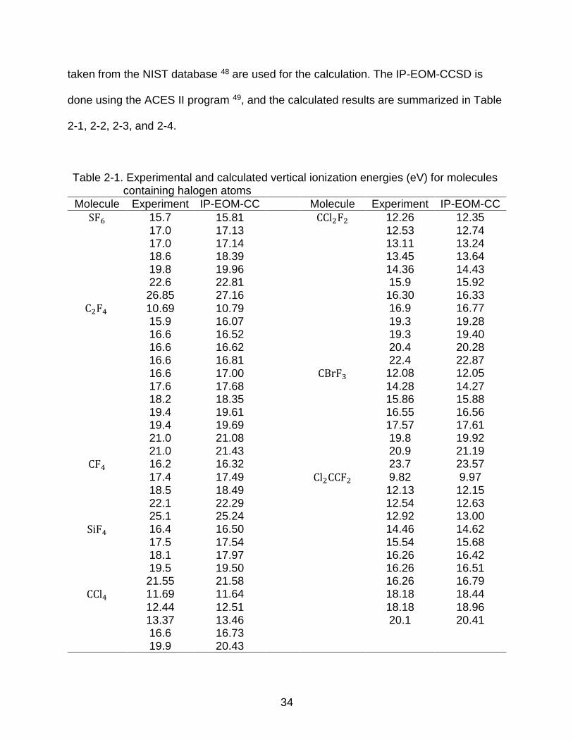
taken from the NIST database 48 are used for the calculation. The IP-EOM-CCSD is

done using the ACES II program 49, and the calculated results are summarized in Table

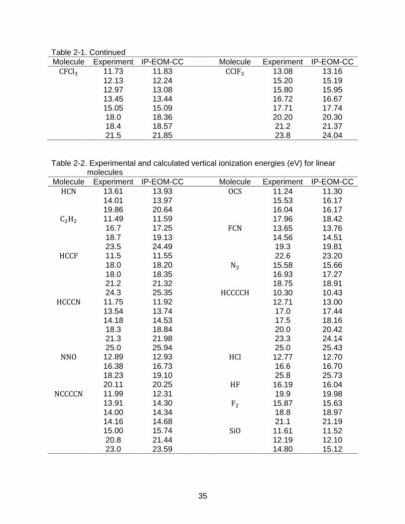
2-1, 2-2, 2-3, and 2-4.

Table 2-1. Experimental and calculated vertical ionization energies (eV) for molecules containing halogen atoms

Molecule Experiment IP-EOM-CC Molecule Experiment IP-EOM-CC

SF6 15.7 15.81 CCl2F2 12.26 12.35 17.0 17.13 12.53 12.74 17.0 17.14 13.11 13.24 18.6 18.39 13.45 13.64 19.8 19.96 14.36 14.43 22.6 22.81 15.9 15.92 26.85 27.16 16.30 16.33

C2F4 10.69 10.79 16.9 16.77

15.9 16.07 19.3 19.28 16.6 16.52 19.3 19.40 16.6 16.62 20.4 20.28 16.6 16.81 22.4 22.87 16.6 17.00 CBrF3 12.08 12.05 17.6 17.68 14.28 14.27 18.2 18.35 15.86 15.88 19.4 19.61 16.55 16.56 19.4 19.69 17.57 17.61 21.0 21.08 19.8 19.92 21.0 21.43 20.9 21.19

CF4 16.2 16.32 23.7 23.57 17.4 17.49 Cl2CCF2 9.82 9.97 18.5 18.49 12.13 12.15 22.1 22.29 12.54 12.63 25.1 25.24 12.92 13.00

SiF4 16.4 16.50 14.46 14.62 17.5 17.54 15.54 15.68 18.1 17.97 16.26 16.42 19.5 19.50 16.26 16.51 21.55 21.58 16.26 16.79

CCl4 11.69 11.64 18.18 18.44

12.44 12.51 18.18 18.96 13.37 13.46 20.1 20.41 16.6 16.73 19.9 20.43

35

Table 2-1. Continued


CFCl3 11.73 11.83 CClF3 13.08 13.16

12.13 12.24 15.20 15.19 12.97 13.08 15.80 15.95 13.45 13.44 16.72 16.67 15.05 15.09 17.71 17.74 18.0 18.36 20.20 20.30 18.4 18.57 21.2 21.37 21.5 21.85 23.8 24.04

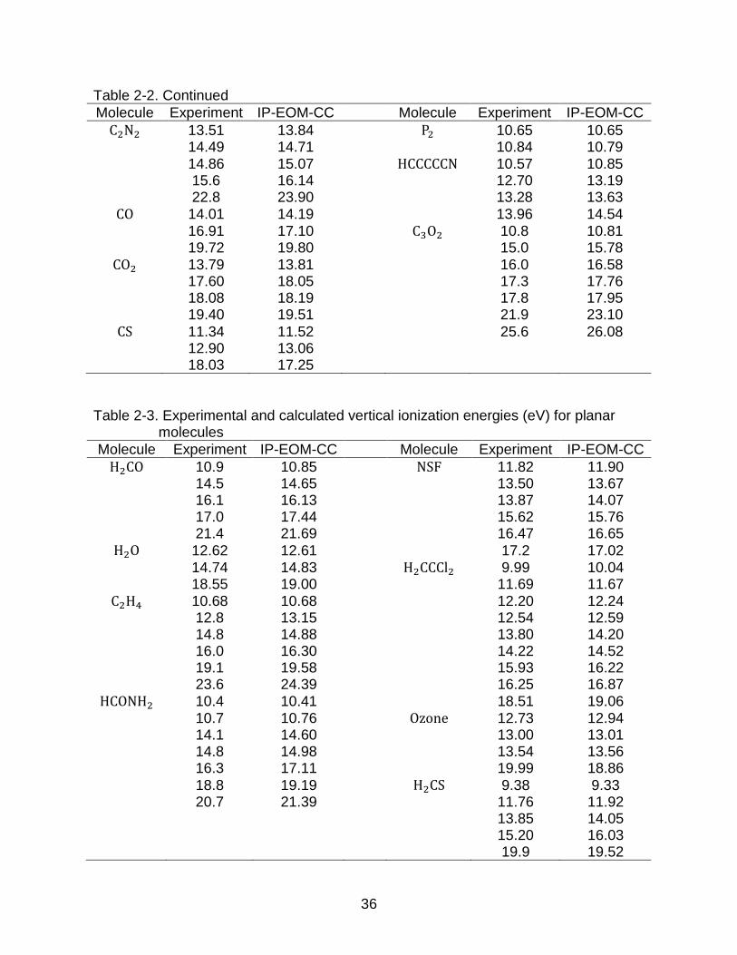
Table 2-2. Experimental and calculated vertical ionization energies (eV) for linear molecules


HCN 13.61 13.93 OCS 11.24 11.30 14.01 13.97 15.53 16.17 19.86 20.64 16.04 16.17

C2H2 11.49 11.59 17.96 18.42 16.7 17.25 FCN 13.65 13.76 18.7 19.13 14.56 14.51 23.5 24.49 19.3 19.81

HCCF 11.5 11.55 22.6 23.20 18.0 18.20 N2 15.58 15.66 18.0 18.35 16.93 17.27 21.2 21.32 18.75 18.91 24.3 25.35 HCCCCH 10.30 10.43

HCCCN 11.75 11.92 12.71 13.00 13.54 13.74 17.0 17.44 14.18 14.53 17.5 18.16 18.3 18.84 20.0 20.42 21.3 21.98 23.3 24.14 25.0 25.94 25.0 25.43

NNO 12.89 12.93 HCl 12.77 12.70 16.38 16.73 16.6 16.70 18.23 19.10 25.8 25.73 20.11 20.25 HF 16.19 16.04

NCCCCN 11.99 12.31 19.9 19.98 13.91 14.30 F2 15.87 15.63 14.00 14.34 18.8 18.97 14.16 14.68 21.1 21.19 15.00 15.74 SiO 11.61 11.52 20.8 21.44 12.19 12.10 23.0 23.59 14.80 15.12

36



C2N2 13.51 13.84 P2 10.65 10.65 14.49 14.71 10.84 10.79 14.86 15.07 HCCCCCN 10.57 10.85 15.6 16.14 12.70 13.19 22.8 23.90 13.28 13.63

CO 14.01 14.19 13.96 14.54 16.91 17.10 C3O2 10.8 10.81 19.72 19.80 15.0 15.78

CO2 13.79 13.81 16.0 16.58 17.60 18.05 17.3 17.76 18.08 18.19 17.8 17.95 19.40 19.51 21.9 23.10

CS 11.34 11.52 25.6 26.08 12.90 13.06 18.03 17.25

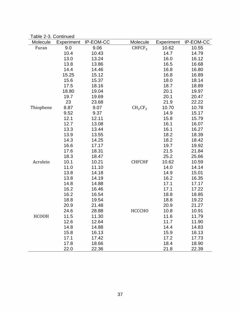
Table 2-3. Experimental and calculated vertical ionization energies (eV) for planar

molecules


H2CO 10.9 10.85 NSF 11.82 11.90 14.5 14.65 13.50 13.67 16.1 16.13 13.87 14.07 17.0 17.44 15.62 15.76 21.4 21.69 16.47 16.65

H2O 12.62 12.61 17.2 17.02 14.74 14.83 H2CCCl2 9.99 10.04 18.55 19.00 11.69 11.67

C2H4 10.68 10.68 12.20 12.24 12.8 13.15 12.54 12.59 14.8 14.88 13.80 14.20 16.0 16.30 14.22 14.52 19.1 19.58 15.93 16.22 23.6 24.39 16.25 16.87

HCONH2 10.4 10.41 18.51 19.06 10.7 10.76 Ozone 12.73 12.94 14.1 14.60 13.00 13.01 14.8 14.98 13.54 13.56 16.3 17.11 19.99 18.86 18.8 19.19 H2CS 9.38 9.33 20.7 21.39 11.76 11.92 13.85 14.05 15.20 16.03 19.9 19.52

37



Furan 9.0 9.06 CHFCF2 10.62 10.55 10.4 10.43 14.7 14.79 13.0 13.24 16.0 16.12 13.8 13.86 16.5 16.68 14.4 14.46 16.8 16.80 15.25 15.12 16.8 16.89 15.6 15.37 18.0 18.14 17.5 18.16 18.7 18.89 18.80 19.04 20.1 19.97 19.7 19.69 20.1 20.47 23 23.68 21.9 22.22

Thiophene 8.87 9.07 CH2CF2 10.70 10.78 9.52 9.37 14.9 15.17 12.1 12.11 15.8 15.79 12.7 13.08 16.1 16.07 13.3 13.44 16.1 16.27 13.9 13.55 18.2 18.39 14.3 14.25 18.2 18.42 16.6 17.17 19.7 19.92 17.6 18.31 21.5 21.84 18.3 18.47 25.2 25.66

Acrolein 10.1 10.21 CHFCHF 10.62 10.59 11.0 11.10 14.0 14.14 13.8 14.18 14.9 15.01 13.8 14.19 16.2 16.35 14.8 14.88 17.1 17.17 16.2 16.46 17.1 17.22 16.2 16.54 18.8 18.85 18.8 19.54 18.8 19.22 20.9 21.48 20.9 21.27 24.6 28.88 HCCCHO 10.8 10.91

HCOOH 11.5 11.30 11.6 11.79 12.6 12.64 11.7 11.90 14.8 14.88 14.4 14.83 15.8 16.13 15.9 16.13 17.1 17.42 17.2 17.73 17.8 18.66 18.4 18.90 22.0 22.36 21.8 22.39

38

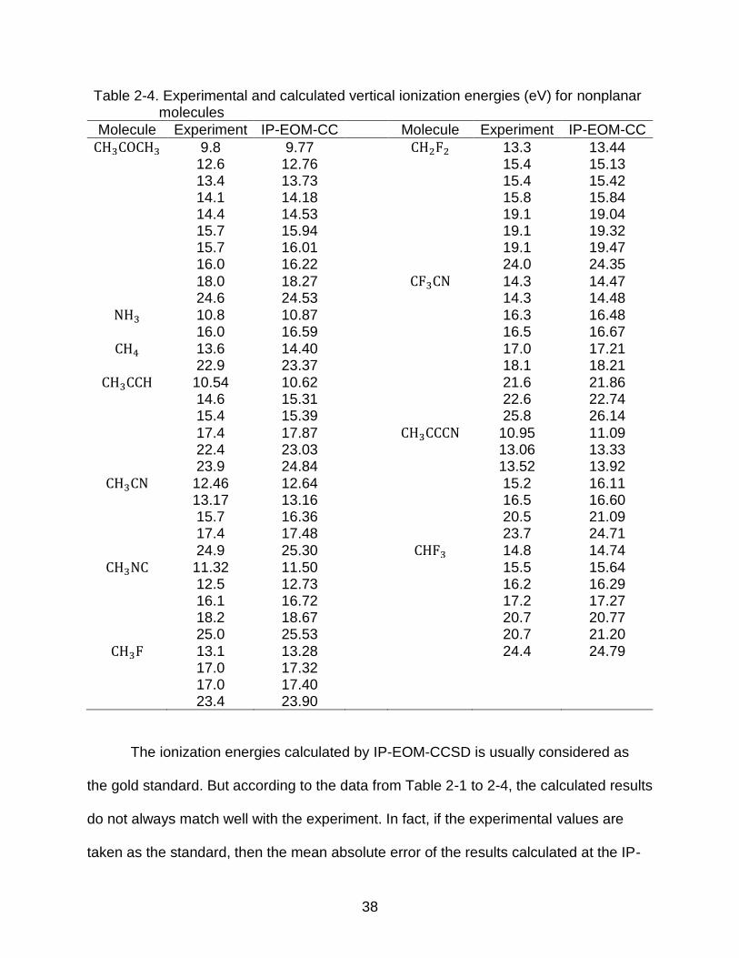
Table 2-4. Experimental and calculated vertical ionization energies (eV) for nonplanar molecules


CH3COCH3 9.8 9.77 CH2F2 13.3 13.44 12.6 12.76 15.4 15.13 13.4 13.73 15.4 15.42 14.1 14.18 15.8 15.84 14.4 14.53 19.1 19.04 15.7 15.94 19.1 19.32 15.7 16.01 19.1 19.47 16.0 16.22 24.0 24.35 18.0 18.27 CF3CN 14.3 14.47 24.6 24.53 14.3 14.48

NH3 10.8 10.87 16.3 16.48 16.0 16.59 16.5 16.67

CH4 13.6 14.40 17.0 17.21 22.9 23.37 18.1 18.21

CH3CCH 10.54 10.62 21.6 21.86 14.6 15.31 22.6 22.74 15.4 15.39 25.8 26.14 17.4 17.87 CH3CCCN 10.95 11.09 22.4 23.03 13.06 13.33 23.9 24.84 13.52 13.92

CH3CN 12.46 12.64 15.2 16.11 13.17 13.16 16.5 16.60 15.7 16.36 20.5 21.09 17.4 17.48 23.7 24.71 24.9 25.30 CHF3 14.8 14.74

CH3NC 11.32 11.50 15.5 15.64 12.5 12.73 16.2 16.29 16.1 16.72 17.2 17.27 18.2 18.67 20.7 20.77 25.0 25.53 20.7 21.20

CH3F 13.1 13.28 24.4 24.79 17.0 17.32 17.0 17.40 23.4 23.90

The ionization energies calculated by IP-EOM-CCSD is usually considered as

the gold standard. But according to the data from Table 2-1 to 2-4, the calculated results

do not always match well with the experiment. In fact, if the experimental values are

taken as the standard, then the mean absolute error of the results calculated at the IP-

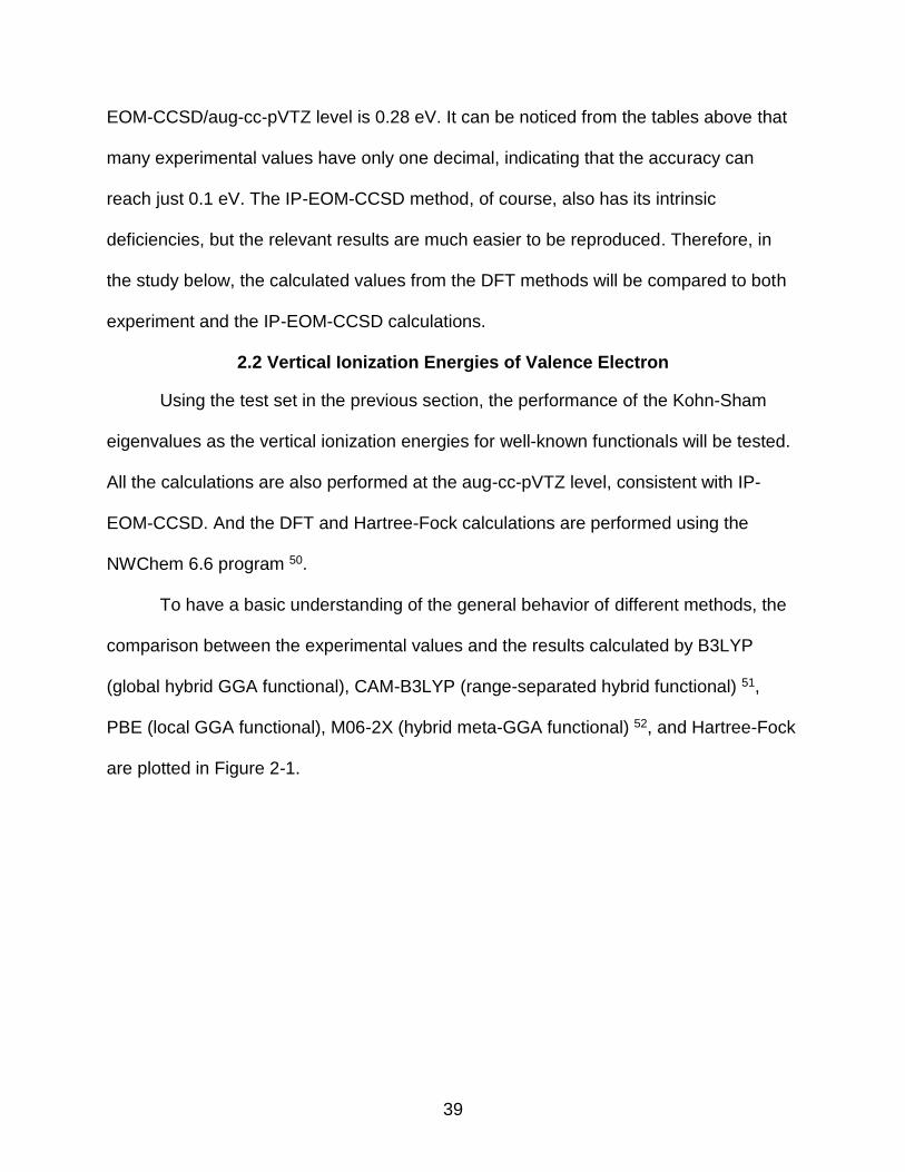
39

EOM-CCSD/aug-cc-pVTZ level is 0.28 eV. It can be noticed from the tables above that

many experimental values have only one decimal, indicating that the accuracy can

reach just 0.1 eV. The IP-EOM-CCSD method, of course, also has its intrinsic

deficiencies, but the relevant results are much easier to be reproduced. Therefore, in

the study below, the calculated values from the DFT methods will be compared to both

experiment and the IP-EOM-CCSD calculations.

2.2 Vertical Ionization Energies of Valence Electron

Using the test set in the previous section, the performance of the Kohn-Sham

eigenvalues as the vertical ionization energies for well-known functionals will be tested.

All the calculations are also performed at the aug-cc-pVTZ level, consistent with IP-

EOM-CCSD. And the DFT and Hartree-Fock calculations are performed using the

NWChem 6.6 program 50.

To have a basic understanding of the general behavior of different methods, the

comparison between the experimental values and the results calculated by B3LYP

(global hybrid GGA functional), CAM-B3LYP (range-separated hybrid functional) 51,

PBE (local GGA functional), M06-2X (hybrid meta-GGA functional) 52, and Hartree-Fock

are plotted in Figure 2-1.

40

Figure 2-1. Comparison between the experimental vertical ionization energies and the computed results by B3LYP, CAM-B3LYP, PBE, M06-2X, and Hartree-Fock

What can be noticed from Figure 2-1 is that although the 58 molecules in the test

set have various physical and chemical properties, the errors of the calculated vertical

ionization energies of a particular method are mostly located inside a small region. For

example, the mean errors for those molecules calculated by the B3LYP method are

primarily located between -2.5 eV to -4 eV, while the errors of M06-2X are mostly

located between -0.5 eV to -1.5 eV.

Taking the experimental measurements and IP-EOM-CCSD calculations as the

reference, the mean absolute errors and the standard deviations of 41 different

functionals and the Hartree-Fock method are summarized in Table 2-5.

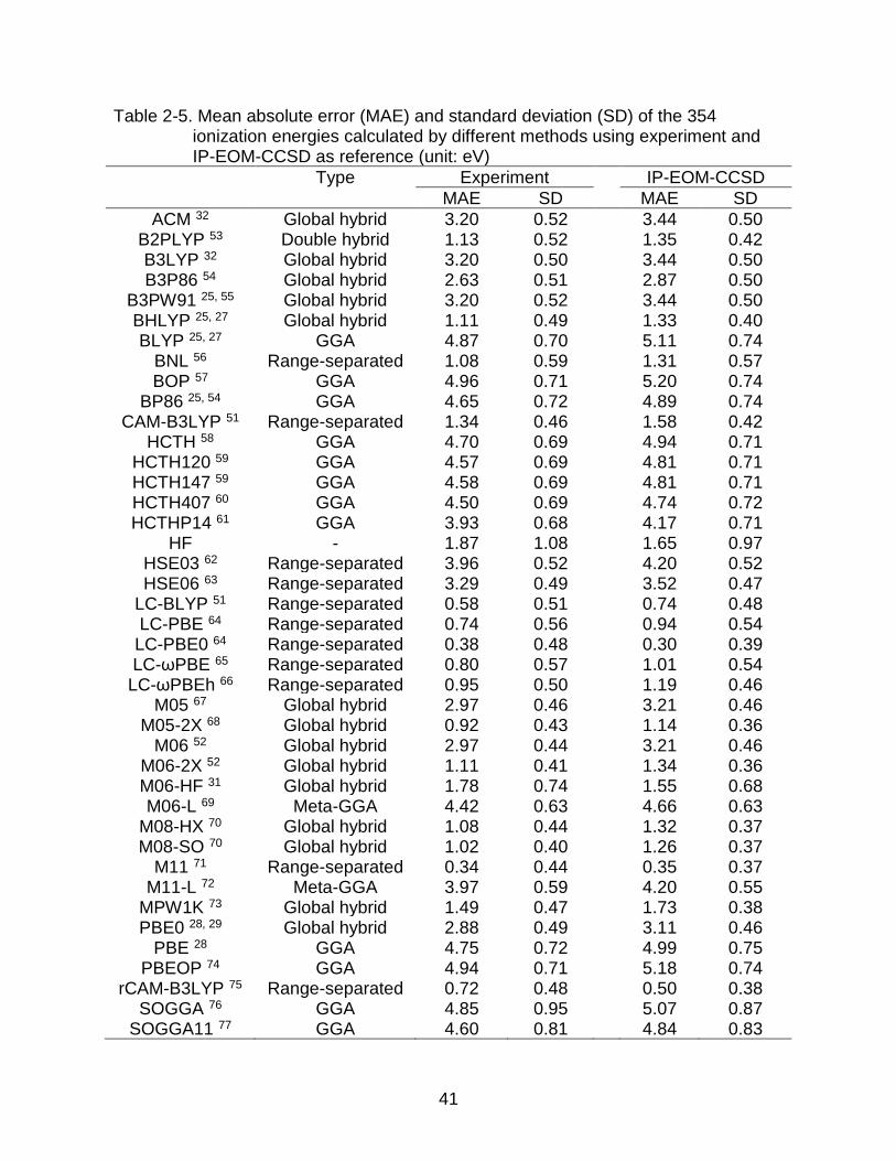
41

Table 2-5. Mean absolute error (MAE) and standard deviation (SD) of the 354 ionization energies calculated by different methods using experiment and IP-EOM-CCSD as reference (unit: eV)

Type Experiment IP-EOM-CCSD

MAE SD MAE SD

ACM 32 Global hybrid 3.20 0.52 3.44 0.50 B2PLYP 53 Double hybrid 1.13 0.52 1.35 0.42 B3LYP 32 Global hybrid 3.20 0.50 3.44 0.50 B3P86 54 Global hybrid 2.63 0.51 2.87 0.50

B3PW91 25, 55 Global hybrid 3.20 0.52 3.44 0.50 BHLYP 25, 27 Global hybrid 1.11 0.49 1.33 0.40 BLYP 25, 27 GGA 4.87 0.70 5.11 0.74

BNL 56 Range-separated 1.08 0.59 1.31 0.57 BOP 57 GGA 4.96 0.71 5.20 0.74

BP86 25, 54 GGA 4.65 0.72 4.89 0.74 CAM-B3LYP 51 Range-separated 1.34 0.46 1.58 0.42

HCTH 58 GGA 4.70 0.69 4.94 0.71 HCTH120 59 GGA 4.57 0.69 4.81 0.71 HCTH147 59 GGA 4.58 0.69 4.81 0.71 HCTH407 60 GGA 4.50 0.69 4.74 0.72 HCTHP14 61 GGA 3.93 0.68 4.17 0.71

HF - 1.87 1.08 1.65 0.97 HSE03 62 Range-separated 3.96 0.52 4.20 0.52 HSE06 63 Range-separated 3.29 0.49 3.52 0.47

LC-BLYP 51 Range-separated 0.58 0.51 0.74 0.48 LC-PBE 64 Range-separated 0.74 0.56 0.94 0.54

LC-PBE0 64 Range-separated 0.38 0.48 0.30 0.39 LC-ωPBE 65 Range-separated 0.80 0.57 1.01 0.54

LC-ωPBEh 66 Range-separated 0.95 0.50 1.19 0.46 M05 67 Global hybrid 2.97 0.46 3.21 0.46

M05-2X 68 Global hybrid 0.92 0.43 1.14 0.36 M06 52 Global hybrid 2.97 0.44 3.21 0.46

M06-2X 52 Global hybrid 1.11 0.41 1.34 0.36 M06-HF 31 Global hybrid 1.78 0.74 1.55 0.68 M06-L 69 Meta-GGA 4.42 0.63 4.66 0.63

M08-HX 70 Global hybrid 1.08 0.44 1.32 0.37 M08-SO 70 Global hybrid 1.02 0.40 1.26 0.37

M11 71 Range-separated 0.34 0.44 0.35 0.37 M11-L 72 Meta-GGA 3.97 0.59 4.20 0.55

MPW1K 73 Global hybrid 1.49 0.47 1.73 0.38 PBE0 28, 29 Global hybrid 2.88 0.49 3.11 0.46

PBE 28 GGA 4.75 0.72 4.99 0.75 PBEOP 74 GGA 4.94 0.71 5.18 0.74

rCAM-B3LYP 75 Range-separated 0.72 0.48 0.50 0.38 SOGGA 76 GGA 4.85 0.95 5.07 0.87

SOGGA11 77 GGA 4.60 0.81 4.84 0.83

42

According to Table 2-5, among all the 41 DFT methods, the Kohn-Sham

eigenvalues of the occupied orbitals for most of the methods could not well reproduce

the exact vertical ionization energies. For some methods, the mean absolute error can

be over 5 eV. Those functionals that have the mean absolute error below 1 eV are all

the hybrid functionals that include a certain amount of non-local exchange. But including

the non-local exchange contribution cannot guarantee that the functional could perform

well for the ionization energies. One of the most popular hybrid functionals, the B3LYP,

has a mean absolute error of 3.20 eV compared to the experiment and 3.44 eV

compared to IP-EOM-CCSD. The local functions such as BLYP, PBE, M06-L, M11-L,

etc. generally have the largest error.

What is interesting from Table 2-5 is that although the mean absolute errors are

quite different, the standard deviations are close to each other. Except for the Hartree-

Fock method which has different origins than the DFT family, the standard deviations for

those functionals are mostly between 0.4 eV and 0.7 eV, much smaller than the desired

1 eV of deviation.

2.3 Vertical Ionization Energies of Core Electron

The energy required to ionize the electrons from the core orbitals is several

magnitudes larger than the valence orbitals, and it is usually located in the X-ray region

on the spectrum. In the experiment, those energies are usually measured through X-ray

photoelectron spectra (XPS) 78. Compared to the ionization energies of the valence

electrons, the accurate computation of the core ionization energies is more challenging.

In this project, the core ionization energies of CH4, C2H2, C2H4, H2CO, NH3, CO,

CO2, HCN, H2O, N2, and HF will be studied. As for the valence ionization energies, the

core ionization energies of the DFT methods are taken as the negative of the

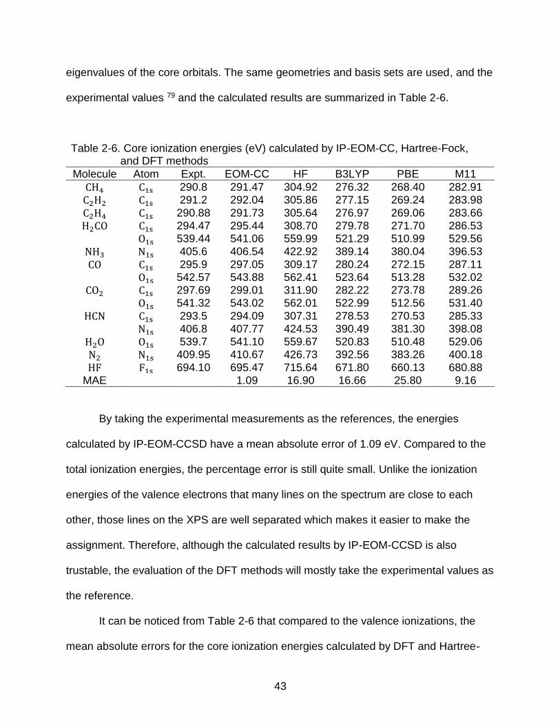
43

eigenvalues of the core orbitals. The same geometries and basis sets are used, and the

experimental values 79 and the calculated results are summarized in Table 2-6.

Table 2-6. Core ionization energies (eV) calculated by IP-EOM-CC, Hartree-Fock, and DFT methods

Molecule Atom Expt. EOM-CC HF B3LYP PBE M11

CH4 C1s 290.8 291.47 304.92 276.32 268.40 282.91

C2H2 C1s 291.2 292.04 305.86 277.15 269.24 283.98

C2H4 C1s 290.88 291.73 305.64 276.97 269.06 283.66

H2CO C1s 294.47 295.44 308.70 279.78 271.70 286.53 O1s 539.44 541.06 559.99 521.29 510.99 529.56

NH3 N1s 405.6 406.54 422.92 389.14 380.04 396.53

CO C1s 295.9 297.05 309.17 280.24 272.15 287.11 O1s 542.57 543.88 562.41 523.64 513.28 532.02

CO2 C1s 297.69 299.01 311.90 282.22 273.78 289.26 O1s 541.32 543.02 562.01 522.99 512.56 531.40

HCN C1s 293.5 294.09 307.31 278.53 270.53 285.33 N1s 406.8 407.77 424.53 390.49 381.30 398.08

H2O O1s 539.7 541.10 559.67 520.83 510.48 529.06

N2 N1s 409.95 410.67 426.73 392.56 383.26 400.18

HF F1s 694.10 695.47 715.64 671.80 660.13 680.88 MAE 1.09 16.90 16.66 25.80 9.16

By taking the experimental measurements as the references, the energies

calculated by IP-EOM-CCSD have a mean absolute error of 1.09 eV. Compared to the

total ionization energies, the percentage error is still quite small. Unlike the ionization

energies of the valence electrons that many lines on the spectrum are close to each

other, those lines on the XPS are well separated which makes it easier to make the

assignment. Therefore, although the calculated results by IP-EOM-CCSD is also

trustable, the evaluation of the DFT methods will mostly take the experimental values as

the reference.

It can be noticed from Table 2-6 that compared to the valence ionizations, the

mean absolute errors for the core ionization energies calculated by DFT and Hartree-

44

Fock methods are much larger. Even for the M11 method, which has excellent

performance for the valence ionization energies, there is still about 9 eV of mean

absolute error for the ionization energies of the core electrons.

The mean absolute errors and standard deviations of computed core ionization

energies are summarized in Table 2-7.

Table 2-7. Mean absolute error (MAE) and standard deviation (SD) of the 15 core ionization energies calculated by different methods (unit: eV)

Method MAE SD Method MAE SD

ACM 17.00 2.25 LC-PBE0 11.91 1.91 B2PLYP 2.63 0.59 LC-ωPBE 21.22 3.46 B3LYP 16.67 2.25 LC-ωPBEH 14.71 2.22 B3P86 16.42 2.22 M05 15.53 2.12

B3PW91 17.01 2.25 M05-2X 4.11 0.64 BHLYP 3.67 0.64 M06 14.78 1.99 BLYP 25.13 3.39 M06-2X 5.13 0.76 BNL 28.94 4.59 M06-HF 8.44 1.53 BOP 25.34 3.42 M06-L 20.74 2.71 BP86 25.33 3.35 M08-HX 5.48 0.82

CAM-B3LYP 14.68 2.26 M08-SO 6.49 0.92 HCTH 25.57 3.60 M11 9.17 1.51

HCTH120 25.50 3.63 M11-L 11.09 1.48 HCTH147 25.64 3.65 MPW1K 7.03 0.94 HCTH407 25.68 3.67 PBE0 15.02 1.92 HCTHP14 26.39 3.83 PBE 25.80 3.41

HF 16.90 2.86 PBEOP 25.56 3.44 HSE03 16.16 1.92 rCAM-B3LYP 12.24 2.21 HSE06 15.39 1.93 SOGGA 27.67 3.65

LC-BLYP 20.55 3.39 SOGGA11 25.15 3.54 LC-PBE 21.64 3.40

Clearly, accurate computation of the core ionization energies is indeed much

more challenging. For most DFT methods, the negative of the Kohn-Sham eigenvalue

deviates greatly from the experiment, and many of them have mean absolute errors

over 20 eV, although some of them perform well for valence ionization energies. For

45

example, the LC-BLYP functional has a mean absolute error of just 0.58 eV for the

valence ionizations (compared to the experiment), the error increases to 20.55 eV for

the core ionizations.

It can also be found from Table 2-7 that the standard deviations are mostly much

smaller than the mean absolute errors, typically below 4 eV. Considering the IP-EOM-

CCSD results can have 1 eV of mean absolute deviation from the experiment, the

standard deviations for the DFT methods are also quite small, similar to the valence

ionizations.

2.4 Discussions

Section 2-2 and 2-3 have shown the performance of the accuracy of the Kohn-

Sham eigenvalues as the vertical ionization energies for various functionals, both the

valence and core electrons. Since the Kohn-Sham eigenvalues generally are not

considered to have a clear physical meaning (except for the HOMO), traditional DFT

methods do not take this property as a training set. And from Table 2-5 and 2-7, the

deviations of the Kohn-Sham eigenvalues from the exact ionization energies are huge

for most of the molecules, especially the core ionizations.

One important point that is worth attention is that although the mean absolute

errors of the different functionals vary greatly, the standard deviations are much closer

to each other. In quantum chemistry, if the mean absolute error for the valence

ionization energy is smaller than 1 eV, the performance of the method is already very

good. And according to Table 2-5, the standard deviations for all the DFT methods are

within 1 eV. For the ionization energies of the core electrons, the mean absolute errors

for most of the functionals are around 2-3 eV, which is fairly small as well compared to

the total energies. This observation implies that if only one molecule in the examples

46

above is taken as the training set to design the new functionals, especially to find the

optimal set of parameters, it should be as reliable as fitting the new method to a large

database of this property.

And this conclusion is one of the most important principles for the ionization

potential improved functionals. In the first version of the functionals in this family, that is,

the CAM-QTP00 and QTP00 (which are the range-separated hybrid and global hybrid

functionals, as will be discussed later), only the water molecule is used as the training

set 80. The negatives of the Kohn-Sham eigenvalues are very close to the exact vertical

ionization energies for the large test set. The physical and chemical properties of the

water molecule have been accurately measured in the experiment. And due to the small

size of the molecule, very large basis set can be used in the theoretical calculation to

ensure the accuracy. At the same time, only a small amount of computing time will be

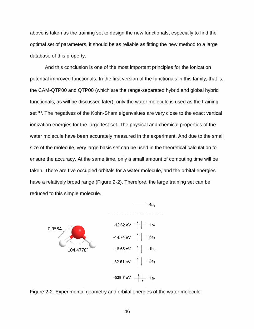
taken. There are five occupied orbitals for a water molecule, and the orbital energies

have a relatively broad range (Figure 2-2). Therefore, the large training set can be

reduced to this simple molecule.

Figure 2-2. Experimental geometry and orbital energies of the water molecule

47

CHAPTER 3 IONIZATION POTENTIAL IMPROVED GLOBAL HYBRID FUNCTIONAL FOR INNER

SHELL EXCITATION ENERGIES

Significant efforts have been made for decades to improve the performance of

DFT methods. Although it is ideal to make the functional “universal”, that is, one

functional could well reproduce all the properties of the atoms and molecules 81, such

kind of method is not available. Instead, each functional will produce a significant error

for one or more properties. And the excitation energies from the inner shell – a property

that is essential to simulate the X-ray absorption spectrum (XAS) 78 – is one of the

examples that is challenging in theoretical chemistry. The XAS is a powerful tool in

chemistry, physics, and material science to determine the structure and other properties

of the molecules.

Since the excitation energies from the inner shells are several orders of

magnitude larger than those from the valence shell, even a small percentage of error

can make the simulated spectra deviate greatly from those measured experimentally.

To match the simulated XAS to the experiment, they often have to be “shifted” to some

degree 82, 83. Obviously, this kind of treatment is somewhat empirical and thus becomes

less trustable by predicting the XAS that is still unknown in the experiment.

The CAM-QTP00, one of the first functionals in the QTP family, could calculate

the excitation energies from the inner-shell with very high accuracy 80, 84. However, the

other ground and excited states properties calculated by CAM-QTP00 have a relatively

large error 85. Also, since the CAM-QTP00 is a range-separated hybrid functional, the

computing cost is somewhat greater than the global hybrid functional. Therefore, it will

be beneficial to create a global hybrid functional that also could accurately reproduce

the inner-shell excitation energies.

48

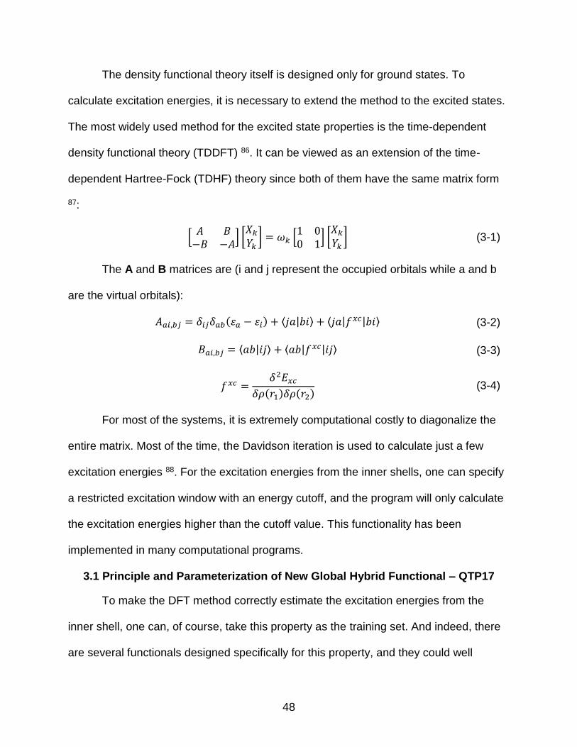
The density functional theory itself is designed only for ground states. To

calculate excitation energies, it is necessary to extend the method to the excited states.

The most widely used method for the excited state properties is the time-dependent

density functional theory (TDDFT) 86. It can be viewed as an extension of the time-

dependent Hartree-Fock (TDHF) theory since both of them have the same matrix form

87:

[𝐴 𝐵

−𝐵 −𝐴] [

𝑋𝑘

𝑌𝑘] = 𝜔𝑘 [

1 00 1

] [𝑋𝑘

𝑌𝑘] (3-1)

The A and B matrices are (i and j represent the occupied orbitals while a and b

are the virtual orbitals):

𝐴𝑎𝑖,𝑏𝑗 = 𝛿𝑖𝑗𝛿𝑎𝑏(휀𝑎 − 휀𝑖) + ⟨𝑗𝑎|𝑏𝑖⟩ + ⟨𝑗𝑎|𝑓𝑥𝑐|𝑏𝑖⟩ (3-2)

𝐵𝑎𝑖,𝑏𝑗 = ⟨𝑎𝑏|𝑖𝑗⟩ + ⟨𝑎𝑏|𝑓𝑥𝑐|𝑖𝑗⟩ (3-3)

𝑓𝑥𝑐 =𝛿2𝐸𝑥𝑐

𝛿𝜌(𝑟1)𝛿𝜌(𝑟2) (3-4)

For most of the systems, it is extremely computational costly to diagonalize the

entire matrix. Most of the time, the Davidson iteration is used to calculate just a few

excitation energies 88. For the excitation energies from the inner shells, one can specify

a restricted excitation window with an energy cutoff, and the program will only calculate

the excitation energies higher than the cutoff value. This functionality has been

implemented in many computational programs.

3.1 Principle and Parameterization of New Global Hybrid Functional – QTP17

To make the DFT method correctly estimate the excitation energies from the

inner shell, one can, of course, take this property as the training set. And indeed, there

are several functionals designed specifically for this property, and they could well

49

reproduce the X-ray absorption spectra 89. However, similar to most of the other

functionals, there is no way to guarantee that they could eventually converge to the

exact answer.

The CAM-QTP00 functional, on the other hand, does not take the inner shell

excitation energies as the training set. Instead, it makes and only makes the negative of

the Kohn-Sham eigenvalues of the five occupied orbitals of the water molecule

approximately equal to the exact ionization potentials. But it could calculate the core

excitation energies of the first-row elements with surprisingly high accuracy. In other

words, the excellent performance of CAM-QTP00 for the core excitation energies is just

a byproduct by enforcing the IP requirement. This conclusion makes sense since

excitation is a process for the electrons transferring from the occupied orbitals to the

virtual orbitals, and thus the energies required for this process should correlate with the

energy differences of the orbitals. Therefore, it can be expected that for a global hybrid

functional, it should also be able to calculate the excitation energies from the inner-shell

accurately by enforcing the IP requirement for the core orbitals.

In fact, there is already a global hybrid functional that is designed to make the

negatives of the Kohn-Sham eigenvalues of all the occupied orbitals (include the core

orbitals) the good approximations to the exact ionization potentials, that is, the QTP00

80. The major problem for the QTP00 is that it is inconsistent since the potential is not

the derivative of the functional:

E𝑥𝑐𝑄𝑇𝑃00 = 𝑎𝐸𝑥

𝐵88 + (1 − 𝑎)𝐸𝑥𝐻𝐹 + 𝑏𝐸𝑐

𝐿𝑌𝑃 (3-5)

V𝑥𝑐𝑄𝑇𝑃00 = 𝑎𝑣𝑥

𝐵88 + (1 − 𝑎)𝑣𝑥𝐻𝐹 + 𝑏𝑣𝑐

𝐿𝑌𝑃 + 𝑐𝑣𝑐𝑉𝑊𝑁 (3-6)

50

Also, the optimized parameters for QTP00 is 𝑎 = 0.45, 𝑏 = 1.00, 𝑐 = 1.17. Clearly, the

summation of b and c does not equal to 1, indicating that too much correlation

contribution is added.

The QTP00 takes the basic formula of B3LYP by removing the LDA exchange

contribution. But in our preliminary test, increasing the percentage of B88 exchange

functional (GGA) could reduce the accuracy of the thermodynamics properties if the IP

theorem is enforced. And since one of the objects of the research is to make the

number of parameters in the new functional as small as possible, we would like to drop

the B88 exchange and instead keep the LDA. The correlation functional will still be the

LYP and VWN. And the summation of the coefficient for both the exchange and

correlation functional should be equal to 1. Therefore, the new functional – QTP17 –

and the potential has the following formula:

E𝑥𝑐𝑄𝑇𝑃17 = 𝑎𝑥𝐸𝑥

𝐻𝐹 + (1 − 𝑎𝑥)𝐸𝑥𝐿𝐷𝐴 + 𝑎𝑐𝐸𝑐

𝐿𝑌𝑃 + (1 − 𝑎𝑐)𝐸𝑐𝑉𝑊𝑁 (3-7)

V𝑥𝑐𝑄𝑇𝑃17 = 𝑎𝑥𝑣𝑥

𝐻𝐹 + (1 − 𝑎𝑥)𝑣𝑥𝐿𝐷𝐴 + 𝑎𝑐𝑣𝑐

𝐿𝑌𝑃 + (1 − 𝑎𝑐)𝑣𝑐𝑉𝑊𝑁 (3-8)

To find the optimal set of parameters 𝑎𝑥 and 𝑎𝑐, we will first use the water

molecule as the training set to make the difference between the calculated orbital

energies and the exact ionization potential smaller than 1 eV. As has been shown in

Chapter 2, the errors coming from the core orbitals are much larger than the valence

orbitals. Therefore, we will not calculate the mean absolute error for all the five orbitals.

Instead, the ionization potential of the 1s orbital and the four valence orbitals will be

evaluated independently. The distribution of the mean absolute error for the valence

orbitals and core orbitals are plotted in Figure 3-1.

51

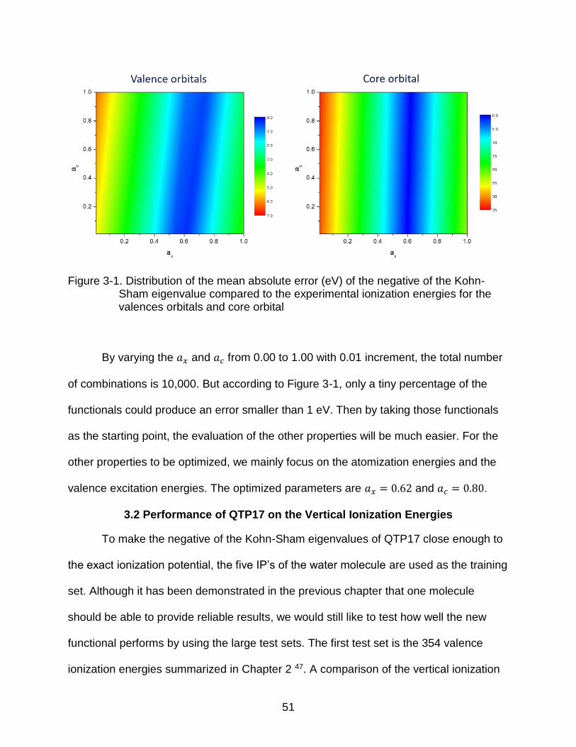
Figure 3-1. Distribution of the mean absolute error (eV) of the negative of the Kohn-Sham eigenvalue compared to the experimental ionization energies for the valences orbitals and core orbital

By varying the 𝑎𝑥 and 𝑎𝑐 from 0.00 to 1.00 with 0.01 increment, the total number

of combinations is 10,000. But according to Figure 3-1, only a tiny percentage of the

functionals could produce an error smaller than 1 eV. Then by taking those functionals

as the starting point, the evaluation of the other properties will be much easier. For the

other properties to be optimized, we mainly focus on the atomization energies and the

valence excitation energies. The optimized parameters are 𝑎𝑥 = 0.62 and 𝑎𝑐 = 0.80.

3.2 Performance of QTP17 on the Vertical Ionization Energies

To make the negative of the Kohn-Sham eigenvalues of QTP17 close enough to

the exact ionization potential, the five IP’s of the water molecule are used as the training

set. Although it has been demonstrated in the previous chapter that one molecule

should be able to provide reliable results, we would still like to test how well the new

functional performs by using the large test sets. The first test set is the 354 valence

ionization energies summarized in Chapter 2 47. A comparison of the vertical ionization

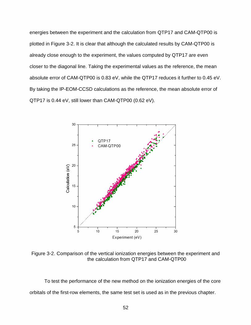
52

energies between the experiment and the calculation from QTP17 and CAM-QTP00 is

plotted in Figure 3-2. It is clear that although the calculated results by CAM-QTP00 is

already close enough to the experiment, the values computed by QTP17 are even

closer to the diagonal line. Taking the experimental values as the reference, the mean

absolute error of CAM-QTP00 is 0.83 eV, while the QTP17 reduces it further to 0.45 eV.

By taking the IP-EOM-CCSD calculations as the reference, the mean absolute error of

QTP17 is 0.44 eV, still lower than CAM-QTP00 (0.62 eV).

Figure 3-2. Comparison of the vertical ionization energies between the experiment and the calculation from QTP17 and CAM-QTP00

To test the performance of the new method on the ionization energies of the core

orbitals of the first-row elements, the same test set is used as in the previous chapter.

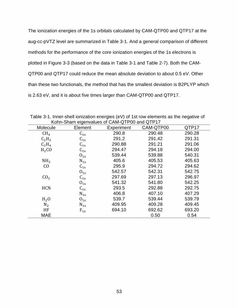
53

The ionization energies of the 1s orbitals calculated by CAM-QTP00 and QTP17 at the

aug-cc-pVTZ level are summarized in Table 3-1. And a general comparison of different

methods for the performance of the core ionization energies of the 1s electrons is

plotted in Figure 3-3 (based on the data in Table 3-1 and Table 2-7). Both the CAM-

QTP00 and QTP17 could reduce the mean absolute deviation to about 0.5 eV. Other

than these two functionals, the method that has the smallest deviation is B2PLYP which

is 2.63 eV, and it is about five times larger than CAM-QTP00 and QTP17.

Table 3-1. Inner-shell ionization energies (eV) of 1st row elements as the negative of Kohn-Sham eigenvalues of CAM-QTP00 and QTP17

Molecule Element Experiment CAM-QTP00 QTP17

CH4 C1s 290.8 290.48 290.28

C2H2 C1s 291.2 291.42 291.31

C2H4 C1s 290.88 291.21 291.06

H2CO C1s 294.47 294.18 294.00 O1s 539.44 539.88 540.31

NH3 N1s 405.6 405.53 405.63

CO C1s 295.9 294.72 294.62 O1s 542.57 542.31 542.75

CO2 C1s 297.69 297.13 296.97 O1s 541.32 541.80 542.25

HCN C1s 293.5 292.88 292.75

N1s 406.8 407.10 407.29

H2O O1s 539.7 539.44 539.79

N2 N1s 409.95 409.28 409.45

HF F1s 694.10 692.62 693.20

MAE 0.50 0.54

54

Figure 3-3. Mean absolute error of core ionization energies of 1s electron computed by different methods

We also tested the inner shell ionization energies of the second-row elements.

To accurately compute the properties of these elements that involve the inner-shells

(1s, 2s, or 2p), the effect of the relativistic effect can be significant. Therefore, the

Douglas-Kroll-Hess relativistic correction is applied, and the basis set aug-cc-pVTZ-DK

is used for the second-row elements. Table 3-2 summarizes the calculated results.

Compared to the first-row elements, the inner shell ionization energies of the second-

row elements are much harder to correctly calculate especially the ionization from the

1s orbitals. But the overall performance of CAM-QTP00 and QTP17 is still satisfactory

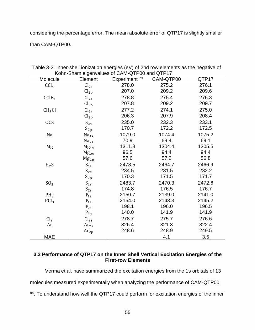
55

considering the percentage error. The mean absolute error of QTP17 is slightly smaller

than CAM-QTP00.

Table 3-2. Inner-shell ionization energies (eV) of 2nd row elements as the negative of Kohn-Sham eigenvalues of CAM-QTP00 and QTP17

Molecule Element Experiment 79 CAM-QTP00 QTP17

CCl4 Cl2s 278.0 275.2 276.1

Cl2p 207.0 209.2 209.6

CClF3 Cl2s 278.8 275.4 276.3 Cl2p 207.8 209.2 209.7

CH3Cl Cl2s 277.2 274.1 275.0 Cl2p 206.3 207.9 208.4

OCS S2s 235.0 232.3 233.1 S2p 170.7 172.2 172.5

Na Na1s 1079.0 1074.4 1075.2 Na2s 70.9 69.4 69.1

Mg Mg1s 1311.3 1304.4 1305.5 Mg2s 96.5 94.4 94.4 Mg2p 57.6 57.2 56.8

H2S S1s 2478.5 2464.7 2466.9

S2s 234.5 231.5 232.2 S2p 170.3 171.5 171.7

SO2 S1s 2483.7 2470.3 2472.6 S2s 174.8 176.5 176.7

PH3 P1s 2150.7 2139.0 2141.0

PCl3 P1s 2154.0 2143.3 2145.2 P2s 198.1 196.0 196.5 P2p 140.0 141.9 141.9

Cl2 Cl2s 278.7 275.7 276.6

Ar Ar2s 326.4 321.3 322.4 Ar2p 248.6 248.9 249.5

MAE 4.1 3.5

3.3 Performance of QTP17 on the Inner Shell Vertical Excitation Energies of the First-row Elements

Verma et al. have summarized the excitation energies from the 1s orbitals of 13

molecules measured experimentally when analyzing the performance of CAM-QTP00

84. To understand how well the QTP17 could perform for excitation energies of the inner

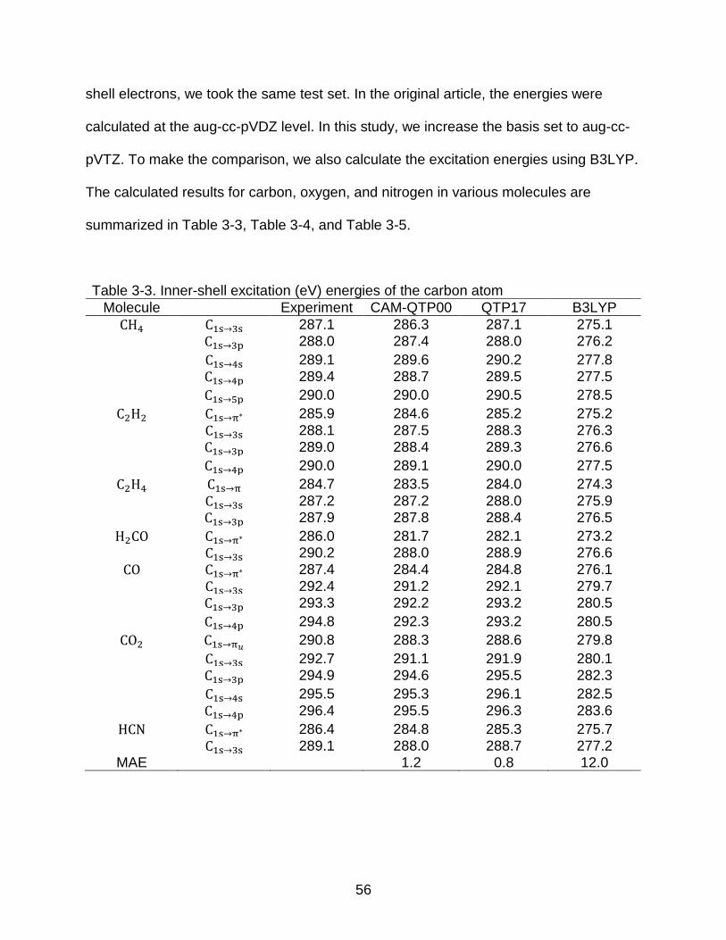
56

shell electrons, we took the same test set. In the original article, the energies were

calculated at the aug-cc-pVDZ level. In this study, we increase the basis set to aug-cc-

pVTZ. To make the comparison, we also calculate the excitation energies using B3LYP.

The calculated results for carbon, oxygen, and nitrogen in various molecules are

summarized in Table 3-3, Table 3-4, and Table 3-5.

Table 3-3. Inner-shell excitation (eV) energies of the carbon atom

Molecule Experiment CAM-QTP00 QTP17 B3LYP

CH4 C1s→3s 287.1 286.3 287.1 275.1 C1s→3p 288.0 287.4 288.0 276.2

C1s→4s 289.1 289.6 290.2 277.8 C1s→4p 289.4 288.7 289.5 277.5

C1s→5p 290.0 290.0 290.5 278.5

C2H2 C1s→π∗ 285.9 284.6 285.2 275.2

C1s→3s 288.1 287.5 288.3 276.3 C1s→3p 289.0 288.4 289.3 276.6

C1s→4p 290.0 289.1 290.0 277.5

C2H4 C1s→π 284.7 283.5 284.0 274.3

C1s→3s 287.2 287.2 288.0 275.9 C1s→3p 287.9 287.8 288.4 276.5

H2CO C1s→π∗ 286.0 281.7 282.1 273.2 C1s→3s 290.2 288.0 288.9 276.6

CO C1s→π∗ 287.4 284.4 284.8 276.1

C1s→3s 292.4 291.2 292.1 279.7

C1s→3p 293.3 292.2 293.2 280.5

C1s→4p 294.8 292.3 293.2 280.5

CO2 C1s→π𝑢 290.8 288.3 288.6 279.8

C1s→3s 292.7 291.1 291.9 280.1 C1s→3p 294.9 294.6 295.5 282.3

C1s→4s 295.5 295.3 296.1 282.5

C1s→4p 296.4 295.5 296.3 283.6

HCN C1s→π∗ 286.4 284.8 285.3 275.7 C1s→3s 289.1 288.0 288.7 277.2

MAE 1.2 0.8 12.0

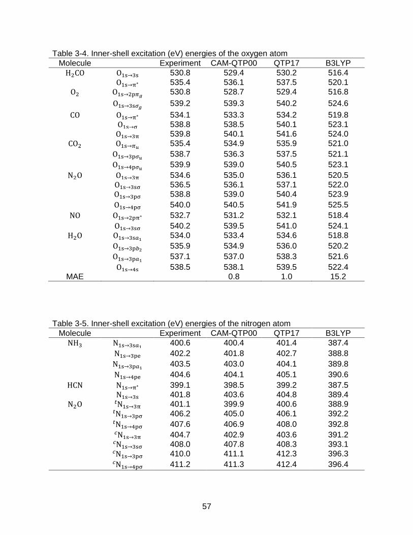
57

Table 3-4. Inner-shell excitation (eV) energies of the oxygen atom


H2CO O1s→3s 530.8 529.4 530.2 516.4

O1s→π∗ 535.4 536.1 537.5 520.1

O2 O1s→2p𝜋𝑔 530.8 528.7 529.4 516.8

O1s→3s𝜎𝑔 539.2 539.3 540.2 524.6

CO O1s→π∗ 534.1 533.3 534.2 519.8 O1s→σ 538.8 538.5 540.1 523.1 O1s→3π 539.8 540.1 541.6 524.0

CO2 O1s→𝜋𝑢 535.4 534.9 535.9 521.0

O1s→3p𝜎𝑢 538.7 536.3 537.5 521.1

O1s→4p𝜎𝑢 539.9 539.0 540.5 523.1

N2O O1s→3π 534.6 535.0 536.1 520.5 O1s→3sσ 536.5 536.1 537.1 522.0 O1s→3pσ 538.8 539.0 540.4 523.9

O1s→4pσ 540.0 540.5 541.9 525.5

NO O1s→2pπ∗ 532.7 531.2 532.1 518.4

O1s→3sσ 540.2 539.5 541.0 524.1

H2O O1s→3s𝑎1 534.0 533.4 534.6 518.8

O1s→3p𝑏2 535.9 534.9 536.0 520.2

O1s→3p𝑎1 537.1 537.0 538.3 521.6

O1s→4s 538.5 538.1 539.5 522.4 MAE 0.8 1.0 15.2

Table 3-5. Inner-shell excitation (eV) energies of the nitrogen atom


NH3 N1s→3s𝑎1 400.6 400.4 401.4 387.4

N1s→3pe 402.2 401.8 402.7 388.8

N1s→3p𝑎1 403.5 403.0 404.1 389.8

N1s→4pe 404.6 404.1 405.1 390.6

HCN N1s→π∗ 399.1 398.5 399.2 387.5 N1s→3s 401.8 403.6 404.8 389.4

N2O N 𝑡

1s→3π 401.1 399.9 400.6 388.9

N 𝑡

1s→3pσ 406.2 405.0 406.1 392.2

N 𝑡

1s→4pσ 407.6 406.9 408.0 392.8

N 𝑐

1s→3π 404.7 402.9 403.6 391.2 N

𝑐1s→3sσ 408.0 407.8 408.3 393.1

N 𝑐

1s→3pσ 410.0 411.1 412.3 396.3

N 𝑐

1s→4pσ 411.2 411.3 412.4 396.4

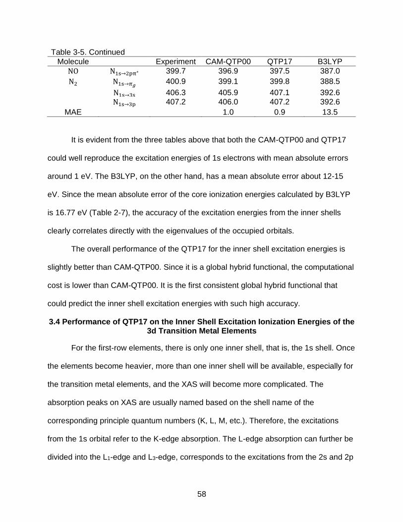
58



NO N1s→2pπ∗ 399.7 396.9 397.5 387.0

N2 N1s→𝜋𝑔 400.9 399.1 399.8 388.5

N1s→3s 406.3 405.9 407.1 392.6 N1s→3p 407.2 406.0 407.2 392.6

MAE 1.0 0.9 13.5

It is evident from the three tables above that both the CAM-QTP00 and QTP17

could well reproduce the excitation energies of 1s electrons with mean absolute errors

around 1 eV. The B3LYP, on the other hand, has a mean absolute error about 12-15

eV. Since the mean absolute error of the core ionization energies calculated by B3LYP

is 16.77 eV (Table 2-7), the accuracy of the excitation energies from the inner shells

clearly correlates directly with the eigenvalues of the occupied orbitals.

The overall performance of the QTP17 for the inner shell excitation energies is

slightly better than CAM-QTP00. Since it is a global hybrid functional, the computational

cost is lower than CAM-QTP00. It is the first consistent global hybrid functional that

could predict the inner shell excitation energies with such high accuracy.

3.4 Performance of QTP17 on the Inner Shell Excitation Ionization Energies of the 3d Transition Metal Elements

For the first-row elements, there is only one inner shell, that is, the 1s shell. Once

the elements become heavier, more than one inner shell will be available, especially for

the transition metal elements, and the XAS will become more complicated. The

absorption peaks on XAS are usually named based on the shell name of the

corresponding principle quantum numbers (K, L, M, etc.). Therefore, the excitations

from the 1s orbital refer to the K-edge absorption. The L-edge absorption can further be

divided into the L1-edge and L3-edge, corresponds to the excitations from the 2s and 2p

59

orbitals, respectively. Obviously, all the excitation energies presented in Section 3.3

correspond to the K-edge absorptions. As it has been shown, the accurate simulation of

this kind of absorption spectra is already a great challenge for DFT methods. In fact,

except for the ionization potential improved functionals in the QTP family, most of the

well know functionals can make over 10 eV error out of the total several hundred

electron volts of energy, consistent with the error of the vertical ionization energies.

As the elements become heavier and heavier, the energy required to excite the

electrons in the 1s orbital will also be higher and higher. At the same time, there will be

more than one inner shell. Thus it will be much more challenging to calculate these

types of excitation energies, especially from the K-edge since the energies required will

be several thousand electron volts or higher.

According to Table 3-2, the negatives of the eigenvalues of CAM-QTP00 and

QTP17 are also close to the exact ionization potentials for the second-row elements

although not as good as the first-row elements. And it will be beneficial if they can also

predict the K-edge and L-edge excitation energies for the heavier elements accurately,

especially the transition metals. Therefore, in this section, the vertical excitation

energies of the 3d transition metal elements will be evaluated.

The experimental values of the inner shell excitation energies of the 3d transition

metal elements are also available 90. All the calculations are done at the aug-cc-pVDZ-

DK level with the Douglas-Kroll-Hess relativistic correction. The computed L3-edge

absorption energies by CAM-QTP00, QTP17, CAM-B3LYP, and B3LYP are

summarized in Table 3-6.

60

Table 3-6. L3-edge absorption energies (eV) of the 3d transition metal elements

Experiment CAM-QTP00 QTP17 CAM-B3LYP B3LYP

Sc 398.7 398.1 399.5 387.5 388.8 Ti 453.8 453.6 455.0 444.9 445.2 V 512.1 512.2 513.6 501.4 503.3 Cr 574.1 574.3 576.0 563.5 564.2 Mn 638.7 641.9 642.0 630.5 630.7 Fe 706.8 707.1 708.9 696.5 697.9 Co 778.1 780.2 782.0 768.9 769.5 Ni 855.0 854.2 856.0 842.4 842.6 Cu 932.0 940.5 943.8 920.6 923.4 Zn 1021 1033 1036 1014 1014

MAE 2.8 4.3 10.0 9.0

The mean absolute error of CAM-QTP00 and QTP17 are acceptable, and the

CAM-QTP00 can give more accurate results. In fact, the calculated values of these two

methods are very close to the experiment from scandium to nickel. The deviation

becomes quite large for the zinc atom. Without considering the zinc, the mean absolute

errors for the other nine elements computed by these two methods are 1.8 eV and 3.1

eV, respectively. The CAM-B3LYP and B3LYP, on the other hand, have much larger

errors.

Table 3-7. K-edge absorption energies (eV) of the 3d transition metal elements

Experiment CAM-QTP00 QTP17 CAM-B3LYP B3LYP

Sc 4493 4463 4467 4416 4333 Ti 4965 4936 4940 4889 4889 V 5465 5434 5438 5383 5385 Cr 5989 5960 5966 5905 5906 Mn 6540 6515 6521 6452 6452 Fe 7112 7075 7080 7020 7021 Co 7709 7672 7677 7618 7615 Ni 8333 8292 8297 8232 8233 Cu 8979 8947 8953 8876 8879 Zn 9659 9628 9635 9557 9558

MAE 32.2 27.1 89.4 97.4

61

Table 3-7 lists the K-edge absorption energies for the 3d transition metal

elements and mean absolute errors. Compared to the L-edge energies, the K-edge

absorption energies are much harder to correctly compute since even scandium has an

excitation energy of 4493 eV. The mean absolute errors of CAM-QTP00 and QTP17 are

around 30 eV, much larger than the L-edge energies (although the percentage errors

are similar). Of course, their overall performance is still much better than other

functionals. The CAM-B3LYP and B3LYP have mean absolute errors of 89 eV and 97

eV, and this error can reach over 100 eV easily for many other methods.

Therefore, it can be concluded that the ionization potential improved functionals

in the QTP family – CAM-QTP00 and QTP17 – show significant improvement for the

inner shell excitation energies of the 3d transition metals, and the L-edge energies are

comparable to experiment. The excitation energies from 1s orbitals have relatively large

deviations from the experiment. Although their performance is better than other DFT

methods, they cannot be used directly in experimental research. A new functional may

need to be designed if one wants to calculate the K-edge absorption energies of the 3d

transition metals without shifting.

3.5 Time Scaling of QTP17 and CAM-QTP00

Based on the results presented in the several previous sections, the QTP17

perform equally well as CAM-QTP00 for the vertical excitation energies, both the

valence and inner shell electrons, but it does not make a significant improvement. The

major advantage of QTP17 is that it is a global hybrid functional and is computationally

more efficient than the range-separated hybrid functionals such as CAM-QTP00. This

section will make a simple test of the scaling of these two methods.

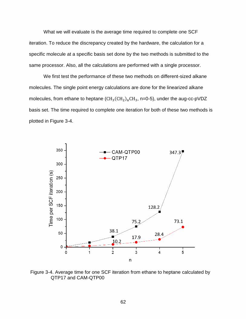
62

What we will evaluate is the average time required to complete one SCF

iteration. To reduce the discrepancy created by the hardware, the calculation for a

specific molecule at a specific basis set done by the two methods is submitted to the

same processor. Also, all the calculations are performed with a single processor.

We first test the performance of these two methods on different-sized alkane

molecules. The single point energy calculations are done for the linearized alkane

molecules, from ethane to heptane (CH3(CH2)nCH3, n=0-5), under the aug-cc-pVDZ

basis set. The time required to complete one iteration for both of these two methods is

plotted in Figure 3-4.

Figure 3-4. Average time for one SCF iteration from ethane to heptane calculated by QTP17 and CAM-QTP00

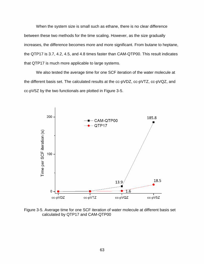
63

When the system size is small such as ethane, there is no clear difference

between these two methods for the time scaling. However, as the size gradually

increases, the difference becomes more and more significant. From butane to heptane,

the QTP17 is 3.7, 4.2, 4.5, and 4.8 times faster than CAM-QTP00. This result indicates

that QTP17 is much more applicable to large systems.

We also tested the average time for one SCF iteration of the water molecule at

the different basis set. The calculated results at the cc-pVDZ, cc-pVTZ, cc-pVQZ, and

cc-pV5Z by the two functionals are plotted in Figure 3-5.

Figure 3-5. Average time for one SCF iteration of water molecule at different basis set calculated by QTP17 and CAM-QTP00

64

A similar trend can be observed as the Figure 3-4. When the basis set is small,

the difference between QTP17 and CAM-QTP00 can almost be neglected. However, as

the basis set becomes larger, the difference also becomes significant. At the cc-pVQZ

basis set, the QTP17 is 8.7 faster than CAM-QTP00. And when the basis set reaches

cc-pV5Z, the QTP17 becomes about 10 times faster.

Therefore, as a global hybrid functional, QTP17 could perform equally well for the

calculation of the vertical ionization and excitation energies as CAM-QTP00, but the

computation is much faster. This feature will enable it to be applied to larger systems

and basis sets.

65

CHAPTER 4 IONIZATION POTENTIAL IMPROVED RANGE-SEPARATED HYBRID EXCHANGE-

CORRELATION FUNCTIONAL １

Although there are thousands of DFT methods published, a lot of them that are

widely used in computational research to reproduce or make predictions of chemical

and physical properties fail in some important applications, such as for Rydberg and

charge transfer excited states 91, 92. In fact, it is a great challenge for time-dependent

density functional theory (TDDFT) to accurately estimate excitation energies. Caricato

et al. and Isegawa et al. did a series of benchmark calculations of 69 singlet excitation

energies from 11 organic molecules using over 50 different functionals 93, 94. The mean

absolute errors summarized in their manuscripts indicate that very few functionals could

accurately reproduce the experimental excitation energies, especially those of Rydberg

states. This is not surprising for at least three obvious reasons: (1) the long-range

asymptotic behavior of the exchange contribution is hard to describe by local functionals

91; (2) Rydberg states have to converge to an ionization continuum, and to facilitate

that, the Kohn-Sham orbital energies need to be good approximations to the principal

ionization energies; and (3) the omnipresent DFT self-interaction error.

The range-separated functionals provide an effective way to help to overcome

some of these deficiencies since 100% (or a very large percentage) of Hartree-Fock

exchange is contributed at long-range so that the potential decay can behave correctly

in that region. However, it is observed in our research that the accuracy of the

calculations is associated with the parameters that determine the range separation and

１ Reproduced from Y. Jin, and R. J. Bartlett, J. Chem. Phys. 145, 034107 (2016), with the permission of AIP Publishing.

66

the amount of non-local exchange contributions. The CAM-QTP00 is one of the

examples of a range-separated functional, and it is powerful at estimating the excitation

energies from the inner shells. However, as it will be shown later, it could not well

reproduce the excitation energies from the valence and Rydberg states as well as many

ground state properties.

This chapter will present a new range-separated hybrid exchange-correlation

functional – CAM-QTP01 – that could significantly improve the accuracy of these

properties.

4.1 Motivation of Range-Separated Exchange Contribution

One of the central problems in density functional theory is to calculate the

exchange energy. It can be calculated either by the exchange functional derived

empirically which depends on the electron density. Or it can be computed using the

Hartree-Fock exchange expression in which the Hartree-Fock orbitals are replaced by

the Kohn-Sham orbitals as Equation 4-1 (closed shell):

𝐸𝑥 = −1

4∑ ∬ 𝜑𝑖

∗(𝑟1)𝜑𝑗∗(𝑟2)𝑟12

−1𝜑𝑗∗(𝑟1)𝜑𝑖

∗(𝑟2)𝑑𝑟1𝑑𝑟2

𝑁

𝑖𝑗

(4-1)

In principle, the exchange energy calculated by Equation 4-1 is much closer to

the exact exchange. However, using the 100% such exchange in combination with the

empirically designed correlation may make the results even worse. The reason is that

the correlation energies calculated by DFT methods are mostly overestimated, and the

exact exchange could not eliminate the error. The local exchange, on the other hand,

can be designed to somewhat underestimate the energy so that the errors caused by

the correlation part can be canceled.

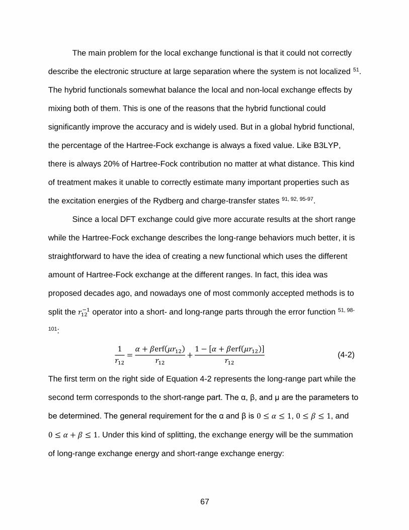
67

The main problem for the local exchange functional is that it could not correctly

describe the electronic structure at large separation where the system is not localized 51.

The hybrid functionals somewhat balance the local and non-local exchange effects by

mixing both of them. This is one of the reasons that the hybrid functional could

significantly improve the accuracy and is widely used. But in a global hybrid functional,

the percentage of the Hartree-Fock exchange is always a fixed value. Like B3LYP,

there is always 20% of Hartree-Fock contribution no matter at what distance. This kind

of treatment makes it unable to correctly estimate many important properties such as

the excitation energies of the Rydberg and charge-transfer states 91, 92, 95-97.

Since a local DFT exchange could give more accurate results at the short range

while the Hartree-Fock exchange describes the long-range behaviors much better, it is

straightforward to have the idea of creating a new functional which uses the different

amount of Hartree-Fock exchange at the different ranges. In fact, this idea was

proposed decades ago, and nowadays one of most commonly accepted methods is to

split the 𝑟12−1 operator into a short- and long-range parts through the error function 51, 98-

101:

1

𝑟12=

𝛼 + 𝛽erf (𝜇𝑟12)

𝑟12+

1 − [𝛼 + 𝛽erf (𝜇𝑟12)]

𝑟12 (4-2)

The first term on the right side of Equation 4-2 represents the long-range part while the

second term corresponds to the short-range part. The α, β, and μ are the parameters to

be determined. The general requirement for the α and β is 0 ≤ 𝛼 ≤ 1, 0 ≤ 𝛽 ≤ 1, and

0 ≤ 𝛼 + 𝛽 ≤ 1. Under this kind of splitting, the exchange energy will be the summation

of long-range exchange energy and short-range exchange energy:

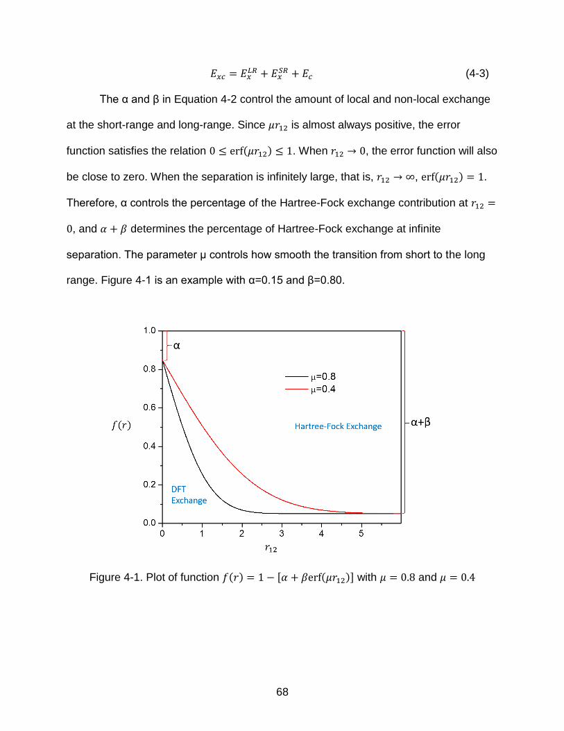
68

𝐸𝑥𝑐 = 𝐸𝑥𝐿𝑅 + 𝐸𝑥

𝑆𝑅 + 𝐸𝑐 (4-3)

The α and β in Equation 4-2 control the amount of local and non-local exchange

at the short-range and long-range. Since 𝜇𝑟12 is almost always positive, the error

function satisfies the relation 0 ≤ erf (𝜇𝑟12) ≤ 1. When 𝑟12 → 0, the error function will also

be close to zero. When the separation is infinitely large, that is, 𝑟12 → ∞, erf(𝜇𝑟12) = 1.

Therefore, α controls the percentage of the Hartree-Fock exchange contribution at 𝑟12 =

0, and 𝛼 + 𝛽 determines the percentage of Hartree-Fock exchange at infinite

separation. The parameter μ controls how smooth the transition from short to the long

range. Figure 4-1 is an example with α=0.15 and β=0.80.

Figure 4-1. Plot of function 𝑓(𝑟) = 1 − [𝛼 + 𝛽erf(𝜇𝑟12)] with 𝜇 = 0.8 and 𝜇 = 0.4

69

In a range-separated functional, the long-range and short-range exchange

energies are calculated independently. The long-range exchange energy uses the same

expression as (3-1) just by replacing the 𝑟12−1 by the first term on the right side of 4-2:

𝐸𝑥𝐿𝑅 = −

1

2∑ ∑ ∬ 𝜑𝑖,𝜎

∗ (𝑟1)𝜑𝑗,𝜎∗ (𝑟2)𝜑𝑗,𝜎

∗𝛼 + 𝛽 erf(𝜇𝑟12)

𝑟12

(𝑟1)𝜑𝑖,𝜎∗ (𝑟2)𝑑𝑟1𝑑𝑟2

𝑖𝑗𝜎

= 𝛼𝐸𝑥𝐻𝐹 −

𝛽

2∑ ∑ ∬ 𝜑𝑖,𝜎

∗ (𝑟1)𝜑𝑗,𝜎∗ (𝑟2)𝜑𝑗,𝜎

∗erf(𝜇𝑟12)

𝑟12

(𝑟1)𝜑𝑖,𝜎∗ (𝑟2)𝑑𝑟1𝑑𝑟2

𝑖𝑗𝜎

(4-4)

The σ in Equation 4-4 represents the α or β spin. The analytical expression for the

short-range exchange energy is more complicated. For the GGA functional, the

exchange energy at the short range is:

𝐸𝑥𝐿𝑅 = −

1

2∑ ∫ 𝜌𝜎

4/3𝐸𝜎

𝐺𝐺𝐴 [(1 − 𝛼) − 𝛽 (8

3𝑎𝜎 (√𝜋erf(2𝑎𝜎)−1 + 2𝑎𝜎(𝑏𝜎 − 𝑐𝜎)))]

𝜎

(4-5)

where the 𝑎𝜎, 𝑏𝜎, and 𝑐𝜎 are defined as:

𝑎𝜎 = 𝜇/(2𝑘𝜎𝐺𝐺𝐴) (4-6)

𝑏𝜎 = 𝑒𝑥 𝑝(−(4𝑎𝜎2)−1 − 1) (4-7)

𝑐𝜎 = 2𝑎𝜎2𝑏𝜎 + 1/2 (4-8)

The 𝑘𝜎𝐺𝐺𝐴 in Equation 4-6 is the Fermi momentum:

𝑘𝜎𝐺𝐺𝐴 = (9𝜋/𝐸𝜎

𝐺𝐺𝐴)1/2𝜌𝜎1/3

(4-9)

By using different functionals and coefficients, various range-separated

functionals can be created 62, 65, 102, 103. This kind of method is usually named as long-

range corrected (LR) functional, especially when α=0 and β=1. It also has the name of

the Coulomb-attenuating method (CAM), which is often used when 𝛼 ≠ 0. The CAM-

B3LYP method, for example, uses B88 for the short-range exchange, and

70

0.81LYP+0.19VWN5 as the correlation 51. In this functional, α=0.19, β=0.46, and

μ=0.33, which is fitted into the atomization energies and total energies.

The CAM-QTP00 functional reparametrized CAM-B3LYP by enforcing the IP

requirement 80. To make the method applicable to other challenging properties such as

Rydberg and charge-transfer excitation energies, we will further optimize the

parameters. Since the new method is one further step from CAM-QTP00, it is thus given

the name as CAM-QTP01.

4.2. Principle and Parameterization of CAM-QTP01 Functional

The correlation functional of CAM-QTP01 is the same as CAM-QTP00

(0.80EcLYP + 0.20Ec

VWN_5). Although the percentage of the EcLYP and Ec

LYP can also be

adjusted, the overall effect for all the properties tested is very small, and hence it is not

necessary to further optimize it. For the exchange part, in order to make the new

functional correctly describe the long-range behaviors of properties, the value of α+β is

restricted to 1. This will guarantee that at the limit that 𝑟12 → ∞, that is, erf(𝜇𝑟12) = 1, the

exchange contribution is represented entirely by a non-local Hartree-Fock equation.

All the KS-DFT calculations are done using the NWChem 6.6 program 50. Most of

the properties are calculated with aug-cc-pVTZ basis set except for excitation energy

calculations, as will be discussed below. In the DFT calculations, the grid is defined as

“xfine” which ensures high accuracy.

Our starting point is still to make the computed ionization energies (the negative

of the Kohn-Sham eigenvalues) of the occupied orbitals close to the experimental

values with errors within 1 eV. The calculations are done at the aug-cc-pVTZ level, and

71

the experimental geometry of the water molecule is also taken from the NIST database

48 (the bond length of O-H is 0.958 Å, and bond angle of H-O-H is 104.4776°).

In our preliminary calculation, we test all combinations of α and β that fulfill the

requirement that 0≤ α≤1, 0≤ β ≤1, and 0≤ α +β ≤1 (the μ is also varied from 0 to 1) with

a precision of 0.01. There were over five thousand sets of parameters that could make

the ionization energies of the water molecule accurate to 1 eV compared with

experiment. However, none of them could significantly increase the accuracy of other

properties such as Rydberg excitation energies, compared to those from CAM-QTP00.

Since the core orbitals in chemistry play a much less significant role than the valence

orbitals, it should still be a good approximation to only consider the IP’s of valence

electrons. Therefore, in the new functional only the first four valence orbitals are taken

into account.

The first parameterization is done on the basis of the experimental excitation

energies of four organic molecules: ethylene, formaldehyde, acetaldehyde, and acetone

(totally 34 states, most of them are Rydberg states). The same geometries in the

original paper by Caricato are used along with the same basis set 6-311(3+,3+)G**. The

vertical excitation energies are calculated by time-dependent density functional theory

(TDDFT), and all the excitations are singlet-singlet excitations (the different states may

belong to different irreducible representations). The mean absolute error (MAE) is

calculated on the basis of the experimental values in the same paper, and the results

are summarized in Figure 4-2. It can be noticed that there is a minimum point on each

curve; as the value of μ increases, the minimum point moves to a smaller α value. The α

value at the minimum point, however, may not be the best value for the error of the

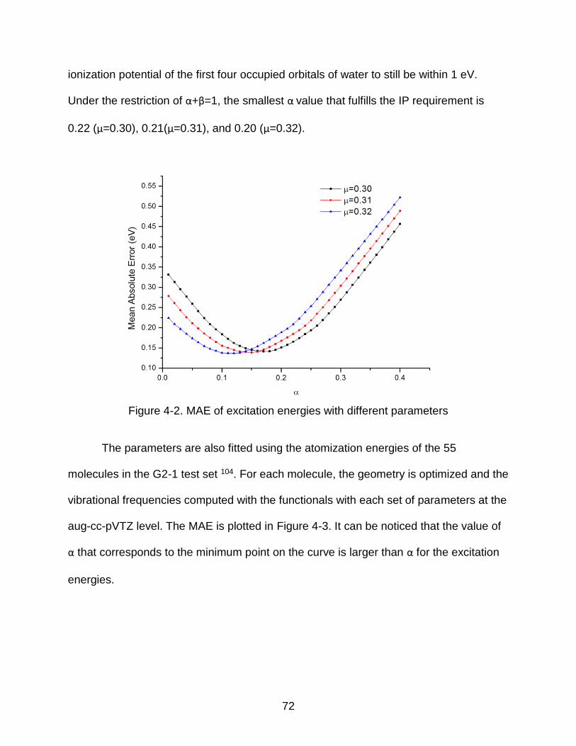
72

ionization potential of the first four occupied orbitals of water to still be within 1 eV.

Under the restriction of α+β=1, the smallest α value that fulfills the IP requirement is

0.22 (μ=0.30), 0.21(μ=0.31), and 0.20 (μ=0.32).

Figure 4-2. MAE of excitation energies with different parameters

The parameters are also fitted using the atomization energies of the 55

molecules in the G2-1 test set 104. For each molecule, the geometry is optimized and the

vibrational frequencies computed with the functionals with each set of parameters at the

aug-cc-pVTZ level. The MAE is plotted in Figure 4-3. It can be noticed that the value of

α that corresponds to the minimum point on the curve is larger than α for the excitation

energies.

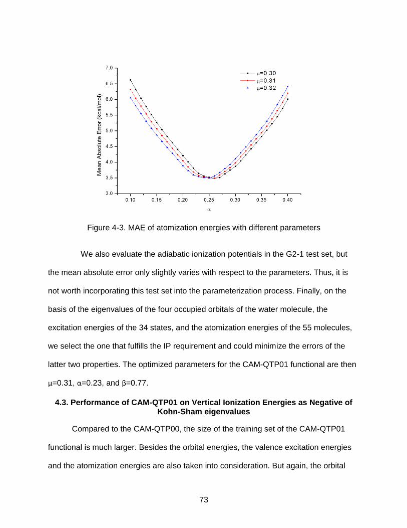
73

Figure 4-3. MAE of atomization energies with different parameters

We also evaluate the adiabatic ionization potentials in the G2-1 test set, but

the mean absolute error only slightly varies with respect to the parameters. Thus, it is

not worth incorporating this test set into the parameterization process. Finally, on the

basis of the eigenvalues of the four occupied orbitals of the water molecule, the

excitation energies of the 34 states, and the atomization energies of the 55 molecules,

we select the one that fulfills the IP requirement and could minimize the errors of the

latter two properties. The optimized parameters for the CAM-QTP01 functional are then

μ=0.31, α=0.23, and β=0.77.

4.3. Performance of CAM-QTP01 on Vertical Ionization Energies as Negative of Kohn-Sham eigenvalues

Compared to the CAM-QTP00, the size of the training set of the CAM-QTP01

functional is much larger. Besides the orbital energies, the valence excitation energies

and the atomization energies are also taken into consideration. But again, the orbital

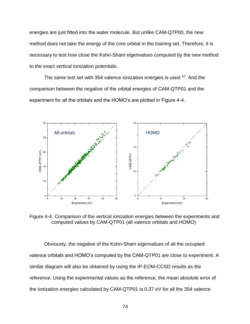
74

energies are just fitted into the water molecule. But unlike CAM-QTP00, the new

method does not take the energy of the core orbital in the training set. Therefore, it is

necessary to test how close the Kohn-Sham eigenvalues computed by the new method

to the exact vertical ionization potentials.

The same test set with 354 valence ionization energies is used 47. And the

comparison between the negative of the orbital energies of CAM-QTP01 and the

experiment for all the orbitals and the HOMO’s are plotted in Figure 4-4.

Figure 4-4. Comparison of the vertical ionization energies between the experiments and computed values by CAM-QTP01 (all valence orbitals and HOMO)

Obviously, the negative of the Kohn-Sham eigenvalues of all the occupied

valence orbitals and HOMO’s computed by the CAM-QTP01 are close to experiment. A

similar diagram will also be obtained by using the IP-EOM-CCSD results as the

reference. Using the experimental values as the reference, the mean absolute error of

the ionization energies calculated by CAM-QTP01 is 0.37 eV for all the 354 valence

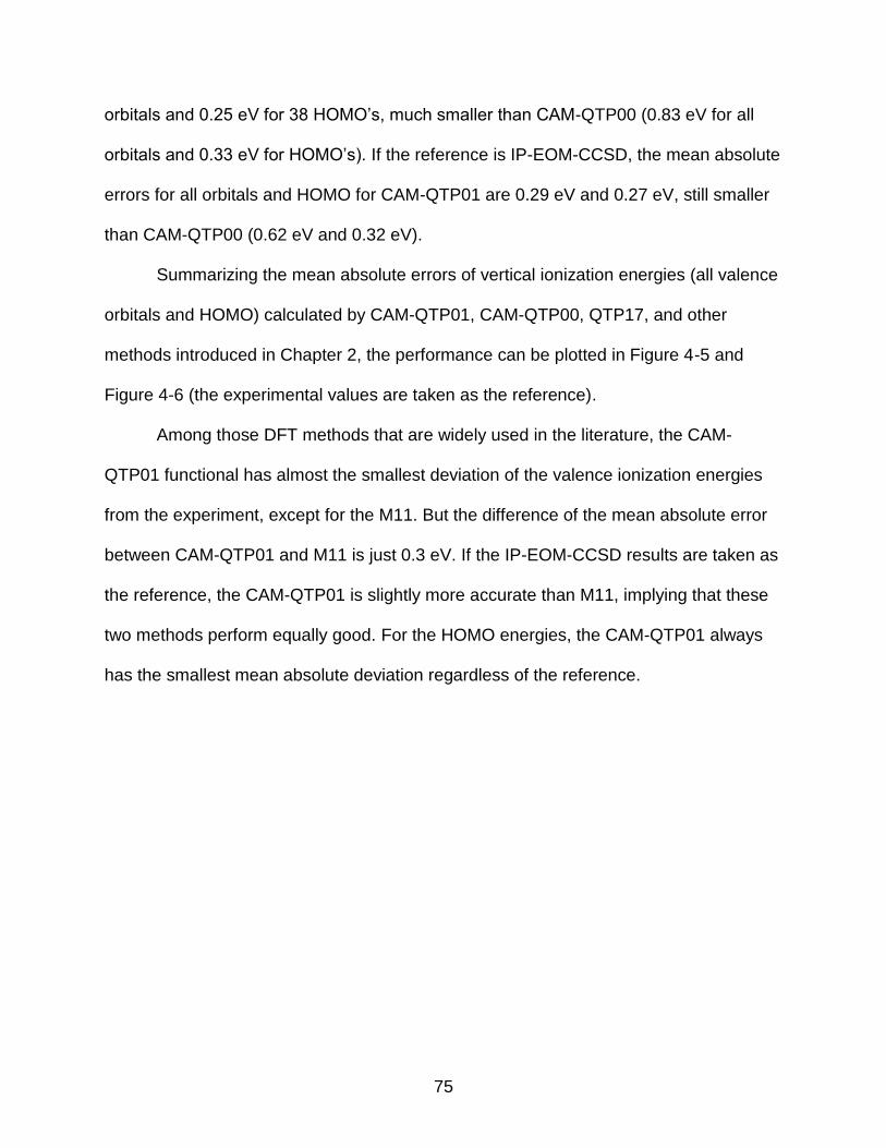
75

orbitals and 0.25 eV for 38 HOMO’s, much smaller than CAM-QTP00 (0.83 eV for all

orbitals and 0.33 eV for HOMO’s). If the reference is IP-EOM-CCSD, the mean absolute

errors for all orbitals and HOMO for CAM-QTP01 are 0.29 eV and 0.27 eV, still smaller

than CAM-QTP00 (0.62 eV and 0.32 eV).

Summarizing the mean absolute errors of vertical ionization energies (all valence

orbitals and HOMO) calculated by CAM-QTP01, CAM-QTP00, QTP17, and other

methods introduced in Chapter 2, the performance can be plotted in Figure 4-5 and

Figure 4-6 (the experimental values are taken as the reference).

Among those DFT methods that are widely used in the literature, the CAM-

QTP01 functional has almost the smallest deviation of the valence ionization energies

from the experiment, except for the M11. But the difference of the mean absolute error

between CAM-QTP01 and M11 is just 0.3 eV. If the IP-EOM-CCSD results are taken as

the reference, the CAM-QTP01 is slightly more accurate than M11, implying that these

two methods perform equally good. For the HOMO energies, the CAM-QTP01 always

has the smallest mean absolute deviation regardless of the reference.

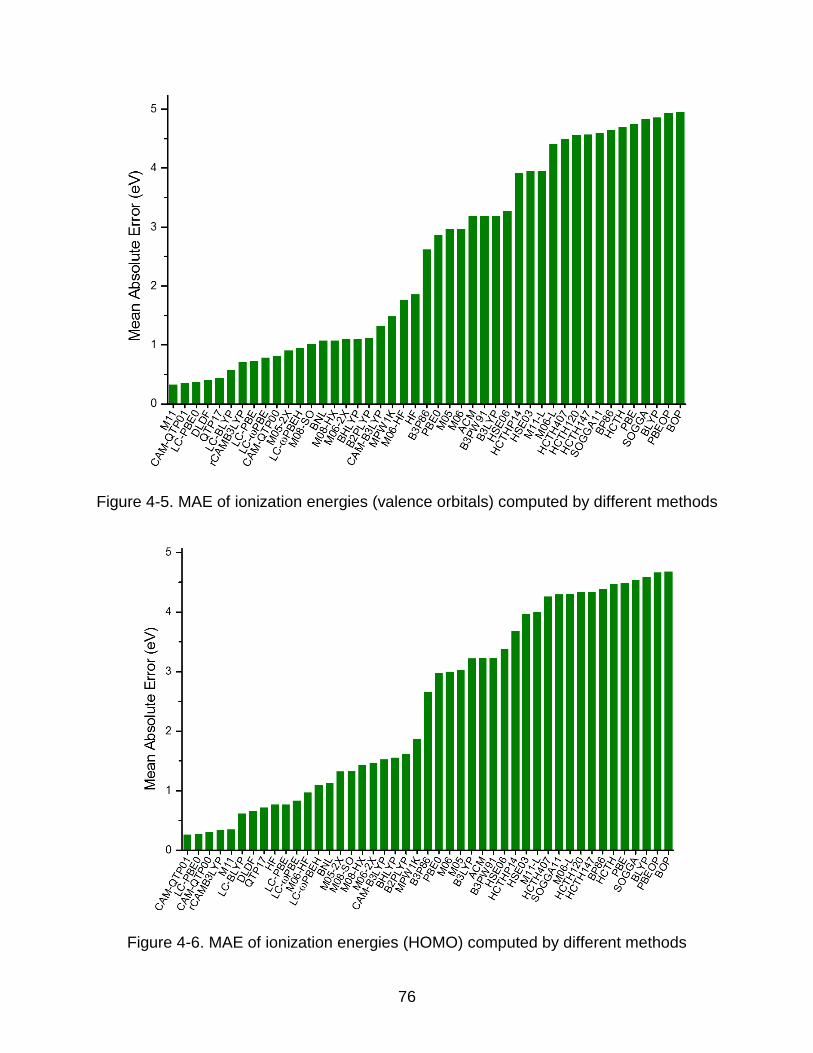
76

Figure 4-5. MAE of ionization energies (valence orbitals) computed by different methods

Figure 4-6. MAE of ionization energies (HOMO) computed by different methods

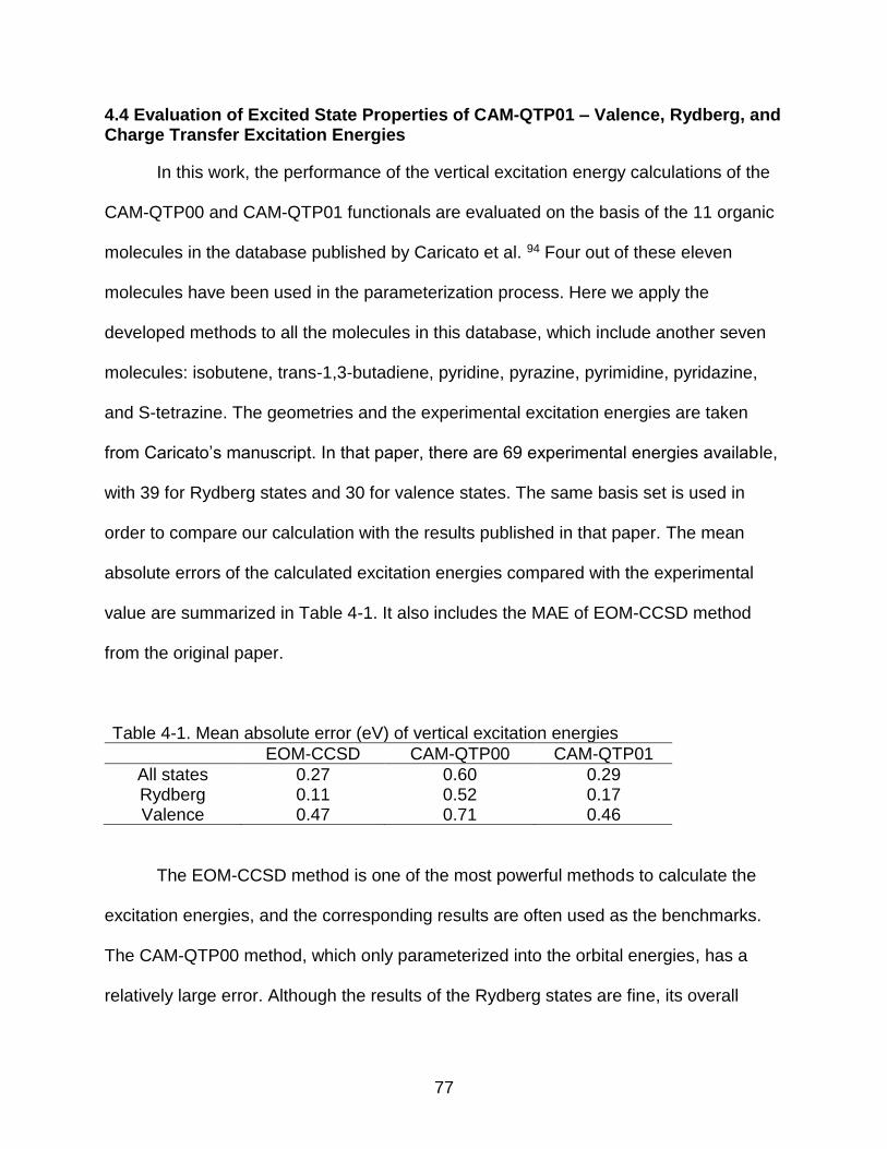
77

4.4 Evaluation of Excited State Properties of CAM-QTP01 – Valence, Rydberg, and Charge Transfer Excitation Energies

In this work, the performance of the vertical excitation energy calculations of the

CAM-QTP00 and CAM-QTP01 functionals are evaluated on the basis of the 11 organic

molecules in the database published by Caricato et al. 94 Four out of these eleven

molecules have been used in the parameterization process. Here we apply the

developed methods to all the molecules in this database, which include another seven

molecules: isobutene, trans-1,3-butadiene, pyridine, pyrazine, pyrimidine, pyridazine,

and S-tetrazine. The geometries and the experimental excitation energies are taken

from Caricato’s manuscript. In that paper, there are 69 experimental energies available,

with 39 for Rydberg states and 30 for valence states. The same basis set is used in

order to compare our calculation with the results published in that paper. The mean

absolute errors of the calculated excitation energies compared with the experimental

value are summarized in Table 4-1. It also includes the MAE of EOM-CCSD method

from the original paper.

Table 4-1. Mean absolute error (eV) of vertical excitation energies

EOM-CCSD CAM-QTP00 CAM-QTP01

All states 0.27 0.60 0.29 Rydberg 0.11 0.52 0.17 Valence 0.47 0.71 0.46

The EOM-CCSD method is one of the most powerful methods to calculate the

excitation energies, and the corresponding results are often used as the benchmarks.

The CAM-QTP00 method, which only parameterized into the orbital energies, has a

relatively large error. Although the results of the Rydberg states are fine, its overall

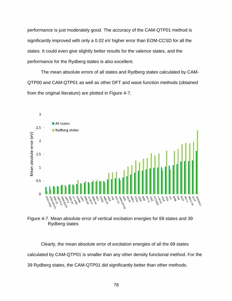
78

performance is just moderately good. The accuracy of the CAM-QTP01 method is

significantly improved with only a 0.02 eV higher error than EOM-CCSD for all the

states. It could even give slightly better results for the valence states, and the

performance for the Rydberg states is also excellent.

The mean absolute errors of all states and Rydberg states calculated by CAM-

QTP00 and CAM-QTP01 as well as other DFT and wave function methods (obtained

from the original literature) are plotted in Figure 4-7.

Figure 4-7. Mean absolute error of vertical excitation energies for 69 states and 39 Rydberg states

Clearly, the mean absolute error of excitation energies of all the 69 states

calculated by CAM-QTP01 is smaller than any other density functional method. For the

39 Rydberg states, the CAM-QTP01 did significantly better than other methods.

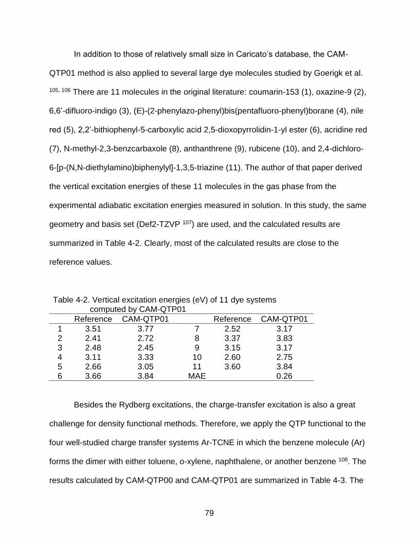
79

In addition to those of relatively small size in Caricato’s database, the CAM-

QTP01 method is also applied to several large dye molecules studied by Goerigk et al.

105, 106 There are 11 molecules in the original literature: coumarin-153 (1), oxazine-9 (2),

6,6’-difluoro-indigo (3), (E)-(2-phenylazo-phenyl)bis(pentafluoro-phenyl)borane (4), nile

red (5), 2,2’-bithiophenyl-5-carboxylic acid 2,5-dioxopyrrolidin-1-yl ester (6), acridine red

(7), N-methyl-2,3-benzcarbaxole (8), anthanthrene (9), rubicene (10), and 2,4-dichloro-

6-[p-(N,N-diethylamino)biphenylyl]-1,3,5-triazine (11). The author of that paper derived

the vertical excitation energies of these 11 molecules in the gas phase from the

experimental adiabatic excitation energies measured in solution. In this study, the same

geometry and basis set (Def2-TZVP 107) are used, and the calculated results are

summarized in Table 4-2. Clearly, most of the calculated results are close to the

reference values.

Table 4-2. Vertical excitation energies (eV) of 11 dye systems computed by CAM-QTP01

Reference CAM-QTP01 Reference CAM-QTP01

1 3.51 3.77 7 2.52 3.17 2 2.41 2.72 8 3.37 3.83 3 2.48 2.45 9 3.15 3.17 4 3.11 3.33 10 2.60 2.75 5 2.66 3.05 11 3.60 3.84 6 3.66 3.84 MAE 0.26

Besides the Rydberg excitations, the charge-transfer excitation is also a great

challenge for density functional methods. Therefore, we apply the QTP functional to the

four well-studied charge transfer systems Ar-TCNE in which the benzene molecule (Ar)

forms the dimer with either toluene, o-xylene, naphthalene, or another benzene 108. The

results calculated by CAM-QTP00 and CAM-QTP01 are summarized in Table 4-3. The

80

mean absolute errors of the four systems calculated by these two functionals as well as

a few other methods are summarized in Figure 4-8. Both CAM-QTP00 and CAM-QTP01

did amazingly well as the calculated results are very close to the experiment. The mean

absolute errors are just 0.08 eV and 0.10 eV respectively. The mean absolute error for

CAM-B3LYP, on the other hand, is about nine times larger.

Table 4-3. Charge transfer excitation energies (eV) of Ar-TCNE systems

QTP17 CAM-QTP00 CAM-QTP01 Experiment

Ar – benzene 3.27 3.77 3.67 3.59 Ar – toluene 2.94 3.44 3.33 3.36 Ar – o-xylene 2.69 3.20 3.08 3.15

Ar – naphthalene 2.15 2.70 2.64 2.60

Figure 4-8. Mean absolute error of charge transfer excitation energies of Ar-TCNE

4.5 Evaluation of Ground States Properties of CAM-QTP01

This section will evaluate the ground states calculated by CAM-QTP00 and CAM-

QTP01, include the geometries (bond lengths and bond angles), vibrational frequencies

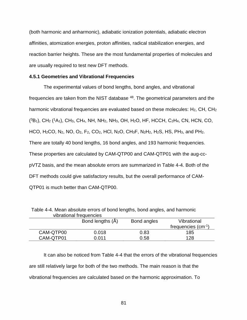
81

(both harmonic and anharmonic), adiabatic ionization potentials, adiabatic electron

affinities, atomization energies, proton affinities, radical stabilization energies, and

reaction barrier heights. These are the most fundamental properties of molecules and

are usually required to test new DFT methods.

4.5.1 Geometries and Vibrational Frequencies

The experimental values of bond lengths, bond angles, and vibrational

frequencies are taken from the NIST database 48. The geometrical parameters and the

harmonic vibrational frequencies are evaluated based on these molecules: H2, CH, CH2

(3B1), CH2 (1A1), CH3, CH4, NH, NH2, NH3, OH, H2O, HF, HCCH, C2H4, CN, HCN, CO,

HCO, H2CO, N2, NO, O2, F2, CO2, HCl, N2O, CH3F, N2H2, H2S, HS, PH3, and PH2.

There are totally 40 bond lengths, 16 bond angles, and 193 harmonic frequencies.

These properties are calculated by CAM-QTP00 and CAM-QTP01 with the aug-cc-

pVTZ basis, and the mean absolute errors are summarized in Table 4-4. Both of the

DFT methods could give satisfactory results, but the overall performance of CAM-

QTP01 is much better than CAM-QTP00.

Table 4-4. Mean absolute errors of bond lengths, bond angles, and harmonic vibrational frequencies

Bond lengths (Å) Bond angles Vibrational frequencies (cm-1)

CAM-QTP00 0.018 0.83 185 CAM-QTP01 0.011 0.58 128

It can also be noticed from Table 4-4 that the errors of the vibrational frequencies

are still relatively large for both of the two methods. The main reason is that the

vibrational frequencies are calculated based on the harmonic approximation. To

82

increase the accuracy, it is necessary to include the anharmonic effect. In this project,

we also calculated the vibrational frequencies with anharmonic correction of these

molecules: CH2 (3B1), CH2 (1A1), CH3, CH4, NH2, H2O, SiH2, SiH3, SiH4, PH2, H2S, C2H4,

HCO, and H2CO. The calculation is done using the “VSCF” module in NWChem

program 50. Since this type of calculation is computationally too costly, it is not practical

to apply it to the larger sized molecules.

Compared with the experimental measurements, the mean absolute error of the

vibrational frequencies with anharmonic correction calculated by CAM-QTP00 is 97.2

cm-1, while for CAM-QTP01 it is 41.8 cm-1. Clearly, the CAM-QTP01 could give more

accurate results. The comparison between the calculated vibrational frequencies and

the experimental values are shown in Figure 4-9. It is clear that the CAM-QTP00 values

are much closer to the experiments.

Figure 4-9. Computed vibrational frequencies with anharmonic corrections compared

with experiments

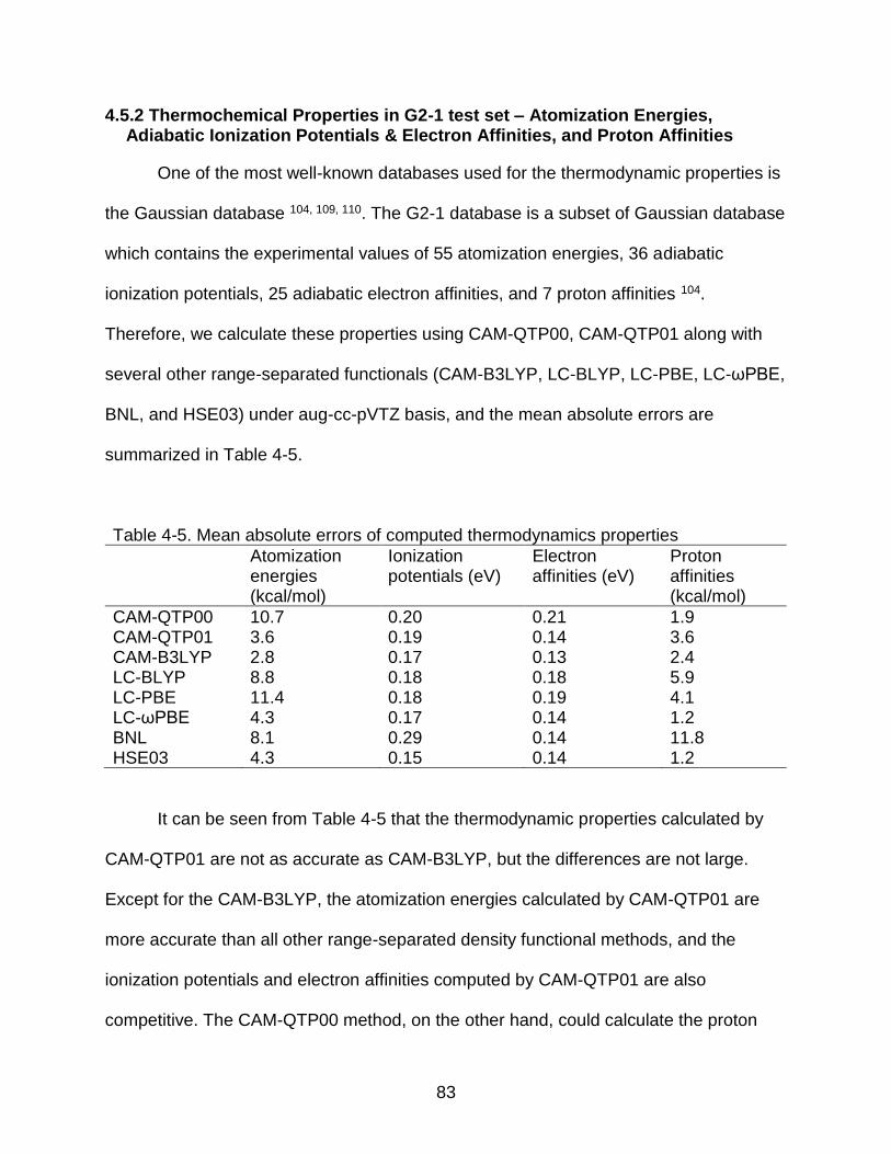
83

4.5.2 Thermochemical Properties in G2-1 test set – Atomization Energies, Adiabatic Ionization Potentials & Electron Affinities, and Proton Affinities

One of the most well-known databases used for the thermodynamic properties is

the Gaussian database 104, 109, 110. The G2-1 database is a subset of Gaussian database

which contains the experimental values of 55 atomization energies, 36 adiabatic

ionization potentials, 25 adiabatic electron affinities, and 7 proton affinities 104.

Therefore, we calculate these properties using CAM-QTP00, CAM-QTP01 along with

several other range-separated functionals (CAM-B3LYP, LC-BLYP, LC-PBE, LC-ωPBE,

BNL, and HSE03) under aug-cc-pVTZ basis, and the mean absolute errors are


Table 4-5. Mean absolute errors of computed thermodynamics properties

Atomization energies (kcal/mol)

Ionization potentials (eV)

Electron affinities (eV)

Proton affinities (kcal/mol)

CAM-QTP00 10.7 0.20 0.21 1.9 CAM-QTP01 3.6 0.19 0.14 3.6 CAM-B3LYP 2.8 0.17 0.13 2.4 LC-BLYP 8.8 0.18 0.18 5.9 LC-PBE 11.4 0.18 0.19 4.1 LC-ωPBE 4.3 0.17 0.14 1.2 BNL 8.1 0.29 0.14 11.8 HSE03 4.3 0.15 0.14 1.2

It can be seen from Table 4-5 that the thermodynamic properties calculated by

CAM-QTP01 are not as accurate as CAM-B3LYP, but the differences are not large.

Except for the CAM-B3LYP, the atomization energies calculated by CAM-QTP01 are

more accurate than all other range-separated density functional methods, and the

ionization potentials and electron affinities computed by CAM-QTP01 are also

competitive. The CAM-QTP00 method, on the other hand, could calculate the proton

84

affinities more accurately than CAM-QTP01 and CAM-B3LYP. One of the reason is that

the CAM-QTP00 calculates the total energies of hydrogen atom very accurately. Since

there is only one electron in the hydrogen atom, there is no correlation effect, and all the

ab initio methods will have the same result under the same basis set. By using the aug-

cc-pVTZ basis, the total energy of the hydrogen atom calculated by the ab initio

methods is -0.499821 Hartree, and the corresponding value calculated by CAM-QTP00

is -0.499895 Hartree which is very close to the ab initio result. The total energies of

hydrogen calculated by CAM-QTP01 and CAM-B3LYP are -0.496477 and -0.498915

Hartree respectively.

It can also be noticed from Table 4-5 that the errors of the atomization energies

computed by CAM-QTP00 are much larger. In fact, among all the 55 atomization

energies calculated by CAM-QTP00, 26 of them have an error greater than 10 kcal/mol.

There are only three molecules that have such a large error for CAM-QTP01. The

comparison between the experimental and computed values of CAM-QTP00 and CAM-

QTP01 are shown in Figure 4-10.

Figure 4-10. Comparison of computed atomization energies with experiments

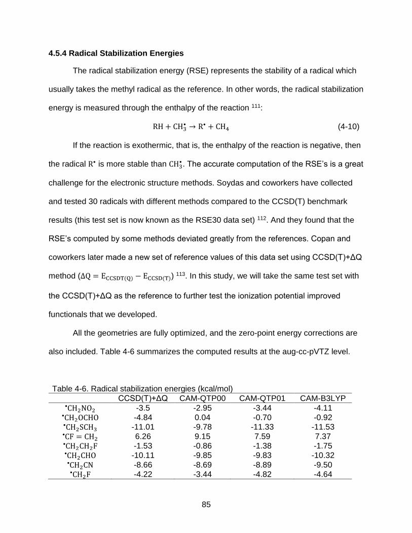
85

4.5.4 Radical Stabilization Energies

The radical stabilization energy (RSE) represents the stability of a radical which

usually takes the methyl radical as the reference. In other words, the radical stabilization

energy is measured through the enthalpy of the reaction 111:

RH + CH3• → R• + CH4 (4-10)

If the reaction is exothermic, that is, the enthalpy of the reaction is negative, then

the radical R• is more stable than CH3• . The accurate computation of the RSE’s is a great

challenge for the electronic structure methods. Soydas and coworkers have collected

and tested 30 radicals with different methods compared to the CCSD(T) benchmark

results (this test set is now known as the RSE30 data set) 112. And they found that the

RSE’s computed by some methods deviated greatly from the references. Copan and

coworkers later made a new set of reference values of this data set using CCSD(T)+ΔQ

method (∆Q = ECCSDT(Q) − ECCSD(T)) 113. In this study, we will take the same test set with

the CCSD(T)+ΔQ as the reference to further test the ionization potential improved

functionals that we developed.

All the geometries are fully optimized, and the zero-point energy corrections are

also included. Table 4-6 summarizes the computed results at the aug-cc-pVTZ level.

Table 4-6. Radical stabilization energies (kcal/mol)

CCSD(T)+ΔQ CAM-QTP00 CAM-QTP01 CAM-B3LYP

CH2 • NO2 -3.5 -2.95 -3.44 -4.11

CH2 • OCHO -4.84 0.04 -0.70 -0.92

CH2 • SCH3 -11.01 -9.78 -11.33 -11.53

CF = • CH2 6.26 9.15 7.59 7.37

CH2 • CH2F -1.53 -0.86 -1.38 -1.75

CH2 • CHO -10.11 -9.85 -9.83 -10.32

CH2 • CN -8.66 -8.69 -8.89 -9.50

CH2 • F -4.22 -3.44 -4.82 -4.64

86


CCSD(T)+ΔQ CAM-QTP00 CAM-QTP01 CAM-B3LYP

CH2 • NH2 -12.06 -12.01 -13.80 -13.65

CH2 • NH3

+ 4.58 3.93 3.55 3.62

CH2 • NHOH -8.81 -8.57 -10.52 -10.57

CH2 • OH -9.27 -8.38 -10.06 -9.79

CH2 • PH3

+ 0.49 1.34 1.15 0.95

CH2 • SH2

+ 2.29 3.04 2.28 2.39

CH2 • SH -9.68 -8.64 -10.03 -10.19

CH2 • C ≡ CH -13.17 -13.54 -14.13 -14.65

CH2 • CH3 -3.36 -3.79 -4.42 -4.53

CH2 • Cl -5.67 -4.89 -6.08 -5.90

CH2 • BH2 -11.66 -9.78 -9.96 -10.35

CHO • -17.61 -14.78 -17.16 -17.05

CH2 • PH2 -6.5 -5.80 -6.64 -6.91

CHClF • -6.61 -4.99 -6.72 -6.65

CHFCH3 • -5.87 -5.47 -6.95 -6.96

CH(OH)2 • -6.67 -6.58 -8.24 -8.27

CHF2 • -9.56 -8.24 -10.02 -9.91

CH2 = C•CH -4.07 -2.68 -4.49 -4.40

C ≡ CH • 1.98 2.13 0.44 -0.81

CH = CH2 • 26.25 32.44 31.87 31.77

CH2CH = CH2 • 5.49 6.73 5.60 5.46

MAE 1.19 0.99 1.05

All the three methods – the CAM-QTP00, CAM-QTP01, and CAM-B3LYP –

perform quite well for the radical stabilization energies with the mean absolute error just

around 1 kcal/mol. It is necessary to emphasize that the CAM-B3LYP method takes a

large database of the thermochemical properties as the training set. The training set for

CAM-QTP01, on the other hand, is much smaller. But the overall performance of radical

stabilization energies for CAM-QTP01 is the same good as CAM-B3LYP. Copan et al.

showed that compared to the reference values of CCSD(T)+ΔQ, even the CCSD(T)

method has the mean absolute error of 0.68 kcal/mol 112. Clearly, the method we

developed could reproduce this property with very high accuracy.

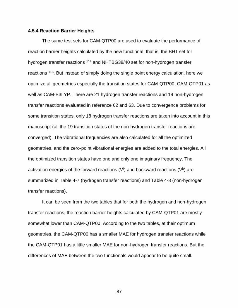
87

4.5.4 Reaction Barrier Heights

The same test sets for CAM-QTP00 are used to evaluate the performance of

reaction barrier heights calculated by the new functional, that is, the BH1 set for

hydrogen transfer reactions 114 and NHTBG38/40 set for non-hydrogen transfer

reactions 115. But instead of simply doing the single point energy calculation, here we

optimize all geometries especially the transition states for CAM-QTP00, CAM-QTP01 as

well as CAM-B3LYP. There are 21 hydrogen transfer reactions and 19 non-hydrogen

transfer reactions evaluated in reference 62 and 63. Due to convergence problems for

some transition states, only 18 hydrogen transfer reactions are taken into account in this

manuscript (all the 19 transition states of the non-hydrogen transfer reactions are

converged). The vibrational frequencies are also calculated for all the optimized

geometries, and the zero-point vibrational energies are added to the total energies. All

the optimized transition states have one and only one imaginary frequency. The

activation energies of the forward reactions (Vf) and backward reactions (Vb) are

summarized in Table 4-7 (hydrogen transfer reactions) and Table 4-8 (non-hydrogen

transfer reactions).

It can be seen from the two tables that for both the hydrogen and non-hydrogen

transfer reactions, the reaction barrier heights calculated by CAM-QTP01 are mostly

somewhat lower than CAM-QTP00. According to the two tables, at their optimum

geometries, the CAM-QTP00 has a smaller MAE for hydrogen transfer reactions while

the CAM-QTP01 has a little smaller MAE for non-hydrogen transfer reactions. But the

differences of MAE between the two functionals would appear to be quite small.

88

CAM-B3LYP, on the other hand, has a mean absolute error of 3.5 kcal/mol for

hydrogen transfer reactions and 3.08 kcal/mol for non-hydrogen transfer reactions,

which are slightly higher than CAM-QTP00 and CAM-QTP01.

Table 4-7. Barrier heights of hydrogen transfer reactions (kcal/mol)

Reactions Best estimate CAM-QTP00 CAM-QTP01 CAM-B3LYP

Vf Vb Vf Vb Vf Vb Vf Vb

Cl+H2↔HCl+H 8.7 5.6 6.1 2.4 0.5 0.1 3.0 0.6 OH+ H2↔H+H2O 5.7 22.0 7.6 16.4 1.9 16.8 2.5 15.0 CH3+H2↔H+CH4 12.1 15.0 13.4 12.1 10.0 11.3 10.9 10.1

OH+CH4↔CH3+H2O 6.7 20.2 9.5 19.6 2.4 16.0 2.4 15.7 H+CH3OH↔CH2OH+H2 7.3 13.8 6.9 16.6 5.1 13.9 4.0 14.6

H+H2↔H2+H 9.6 9.6 5.9 5.9 4.2 4.2 2.8 2.8 OH+NH3↔H2O+NH2 3.2 13.2 8.8 17.7 0.7 11.5 -0.3 10.7 HCl+CH3↔Cl+CH4 1.8 7.8 3.5 6.0 0.6 2.3 1.0 2.7

OH+C2H6↔H2O+C2H5 3.4 20.7 6.6 20.5 0.5 18.5 0.4 18.2 OH+CH3↔O+CH4 7.8 13.7 10.1 13.6 6.1 5.8 6.3 5.3 H+PH3↔PH2+H2 3.2 25.2 1.5 24.9 0.6 22.4 0.6 24.2 H+ClH↔HCl+H 18.0 18.0 17.7 17.7 15.4 15.4 14.3 14.3 H+H2S↔H2+HS 3.6 17.4 1.9 17.5 0.8 14.0 0.8 15.8 O+HCl↔OH+Cl 9.8 9.9 11.9 10.9 3.9 6.0 3.0 5.5

CH4+NH↔NH2+CH3 22.7 8.4 23.4 12.3 17.8 8.2 17.8 8.6 C2H6+NH↔NH2+C2H5 18.4 8.0 20.1 12.7 14.4 9.2 14.3 9.5 C2H6+NH2↔NH3+C2H5 10.4 17.8 15.0 19.9 9.3 16.5 9.7 16.4 NH2+CH4↔CH3+NH3 14.5 17.9 18.0 19.1 12.3 15.1 12.6 15.0

Mean absolute error 2.2 3.3 3.5

Table 4-8. Barrier heights of non-hydrogen transfer reactions (kcal/mol)


Vf Vb Vf Vb Vf Vb Vf Vb

H+N2O↔OH+N2 18.14 83.22 17.50 93.13 14.25 77.52 13.62 76.41 H+FH↔HF+H 42.18 42.18 37.80 37.80 32.30 32.30 30.83 30.83

H+ClH↔HCl+H 18.00 18.00 17.18 17.18 14.87 14.87 13.88 13.88 H+FCH3↔HF+CH3 30.38 57.02 32.63 59.33 27.72 51.47 25.03 50.62

H+F2↔HF+F 2.27 106.18 2.16 114.56 0.42 99.29 0.07 98.36 CH3+FCl↔CH3F+Cl 7.43 60.17 11.35 65.68 7.31 58.48 5.13 54.89 F-+CH3F↔FCH3+F- -0.34 -0.34 1.86 1.86 -1.23 -1.23 -1.45 -1.45 F-…CH3F↔FCH3

…F- 13.38 13.38 15.74 15.74 13.15 13.15 11.39 11.39 Cl-+CH3Cl↔ClCH3+Cl- 3.1 3.1 4.36 4.36 3.57 3.57 2.07 2.07 Cl-…CH3Cl↔ClCH3

…Cl- 13.61 13.61 14.49 14.49 13.98 13.98 11.37 11.37 F-+CH3Cl↔FCH3+Cl- -12.54 20.11 -12.54 25.21 -13.04 21.14 -13.41 19.75

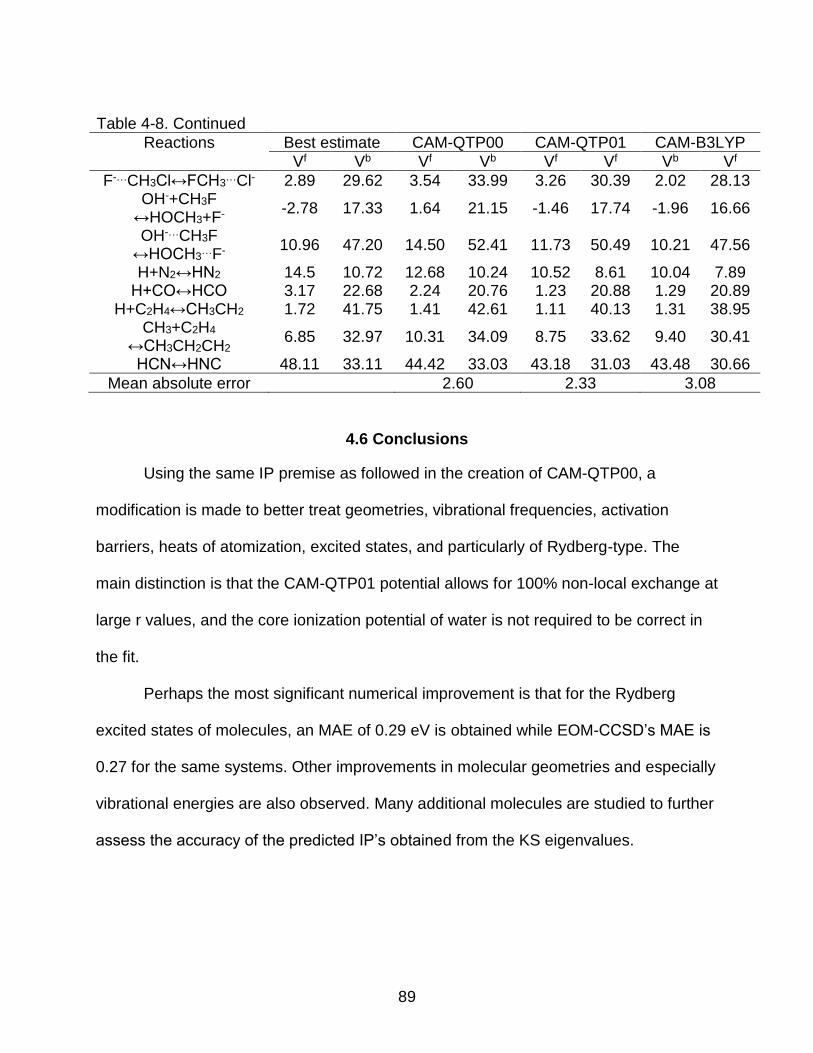
89



Vf Vb Vf Vb Vf Vf Vb Vf

F-…CH3Cl↔FCH3…Cl- 2.89 29.62 3.54 33.99 3.26 30.39 2.02 28.13

OH-+CH3F ↔HOCH3+F-

-2.78 17.33 1.64 21.15 -1.46 17.74 -1.96 16.66

OH-…CH3F ↔HOCH3

…F- 10.96 47.20 14.50 52.41 11.73 50.49 10.21 47.56

H+N2↔HN2 14.5 10.72 12.68 10.24 10.52 8.61 10.04 7.89 H+CO↔HCO 3.17 22.68 2.24 20.76 1.23 20.88 1.29 20.89

H+C2H4↔CH3CH2 1.72 41.75 1.41 42.61 1.11 40.13 1.31 38.95 CH3+C2H4

↔CH3CH2CH2 6.85 32.97 10.31 34.09 8.75 33.62 9.40 30.41

HCN↔HNC 48.11 33.11 44.42 33.03 43.18 31.03 43.48 30.66

Mean absolute error 2.60 2.33 3.08

4.6 Conclusions

Using the same IP premise as followed in the creation of CAM-QTP00, a

modification is made to better treat geometries, vibrational frequencies, activation

barriers, heats of atomization, excited states, and particularly of Rydberg-type. The

main distinction is that the CAM-QTP01 potential allows for 100% non-local exchange at

large r values, and the core ionization potential of water is not required to be correct in

the fit.

Perhaps the most significant numerical improvement is that for the Rydberg

excited states of molecules, an MAE of 0.29 eV is obtained while EOM-CCSD’s MAE is

0.27 for the same systems. Other improvements in molecular geometries and especially

vibrational energies are also observed. Many additional molecules are studied to further

assess the accuracy of the predicted IP’s obtained from the KS eigenvalues.

90

CHAPTER 5 CAN IONIZATION POTENTIAL IMPROVED DENSITY FUNCTIONAL THEORY

REDUCE THE SELF-INTERACTION ERROR?

During the recent decades, the number of new density functional methods grows

almost exponentially every year. Although they are designed to get the right answer

without a solid theoretical foundation (e.g. many of them just force the method itself to

reproduce the properties measured experimentally), they indeed have made a great

contribution to the modern scientific research. However, since the exchange-correlation

functionals are not built upon rigorous derivations, they suffer some serious problems,

for example, the self-interaction error 24. And it is one of the biggest challenges in

designing new functionals. This chapter will demonstrate the performance of the

ionization potential improved functionals to reduce the self-interaction error.

5.1 What is the Self-interaction error?

As has been mentioned in Chapter 1, the total energy of a system is the

summation of the kinetic energy, electron-nucleus attraction potential, and electron-

electron repulsion potential. And the last term – electron-electron repulsion – is the

interparticle interaction, that is, an electron cannot interact with itself, and the

corresponding potential must be zero. Particularly, in a system where there is only one

electron, the third term in Equation 1-3 will disappear, and the total energy will be:

𝐸1𝑒 = ⟨Ψ0|�̂� + �̂�𝑁𝑒|Ψ0⟩ = ⟨Ψ0|−12 ∇1

2 − ∑𝑍𝐴

𝑟1𝐴𝐴 |Ψ0⟩ (5-1)

In Hartree-Fock theory, the total energy is:

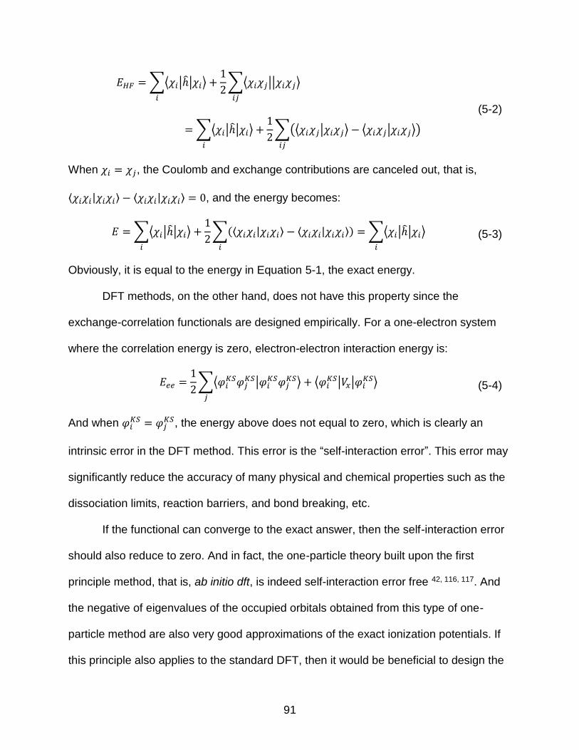
91

𝐸𝐻𝐹 = ∑⟨𝜒𝑖|ℎ̂|𝜒𝑖⟩

𝑖

+1

2∑⟨𝜒𝑖𝜒𝑗||𝜒𝑖𝜒𝑗⟩

𝑖𝑗

= ∑⟨𝜒𝑖|ℎ̂|𝜒𝑖⟩

𝑖

+1

2∑(⟨𝜒𝑖𝜒𝑗|𝜒𝑖𝜒𝑗⟩ − ⟨𝜒𝑖𝜒𝑗|𝜒𝑖𝜒𝑗⟩)

𝑖𝑗

(5-2)

When 𝜒𝑖 = 𝜒𝑗, the Coulomb and exchange contributions are canceled out, that is,

⟨𝜒𝑖𝜒𝑖|𝜒𝑖𝜒𝑖⟩ − ⟨𝜒𝑖𝜒𝑖|𝜒𝑖𝜒𝑖⟩ = 0, and the energy becomes:

𝐸 = ∑⟨𝜒𝑖|ℎ̂|𝜒𝑖⟩

𝑖

+1

2∑(⟨𝜒𝑖𝜒𝑖|𝜒𝑖𝜒𝑖⟩ − ⟨𝜒𝑖𝜒𝑖|𝜒𝑖𝜒𝑖⟩)

𝑖

= ∑⟨𝜒𝑖|ℎ̂|𝜒𝑖⟩

𝑖

(5-3)

Obviously, it is equal to the energy in Equation 5-1, the exact energy.

DFT methods, on the other hand, does not have this property since the

exchange-correlation functionals are designed empirically. For a one-electron system

where the correlation energy is zero, electron-electron interaction energy is:

𝐸𝑒𝑒 =1

2∑⟨𝜑𝑖

𝐾𝑆𝜑𝑗𝐾𝑆|𝜑𝑖

𝐾𝑆𝜑𝑗𝐾𝑆⟩

𝑗

+ ⟨𝜑𝑖𝐾𝑆|𝑉𝑥|𝜑𝑖

𝐾𝑆⟩ (5-4)

And when 𝜑𝑖𝐾𝑆 = 𝜑𝑗

𝐾𝑆, the energy above does not equal to zero, which is clearly an

intrinsic error in the DFT method. This error is the “self-interaction error”. This error may

significantly reduce the accuracy of many physical and chemical properties such as the

dissociation limits, reaction barriers, and bond breaking, etc.

If the functional can converge to the exact answer, then the self-interaction error

should also reduce to zero. And in fact, the one-particle theory built upon the first

principle method, that is, ab initio dft, is indeed self-interaction error free 42, 116, 117. And

the negative of eigenvalues of the occupied orbitals obtained from this type of one-

particle method are also very good approximations of the exact ionization potentials. If

this principle also applies to the standard DFT, then it would be beneficial to design the

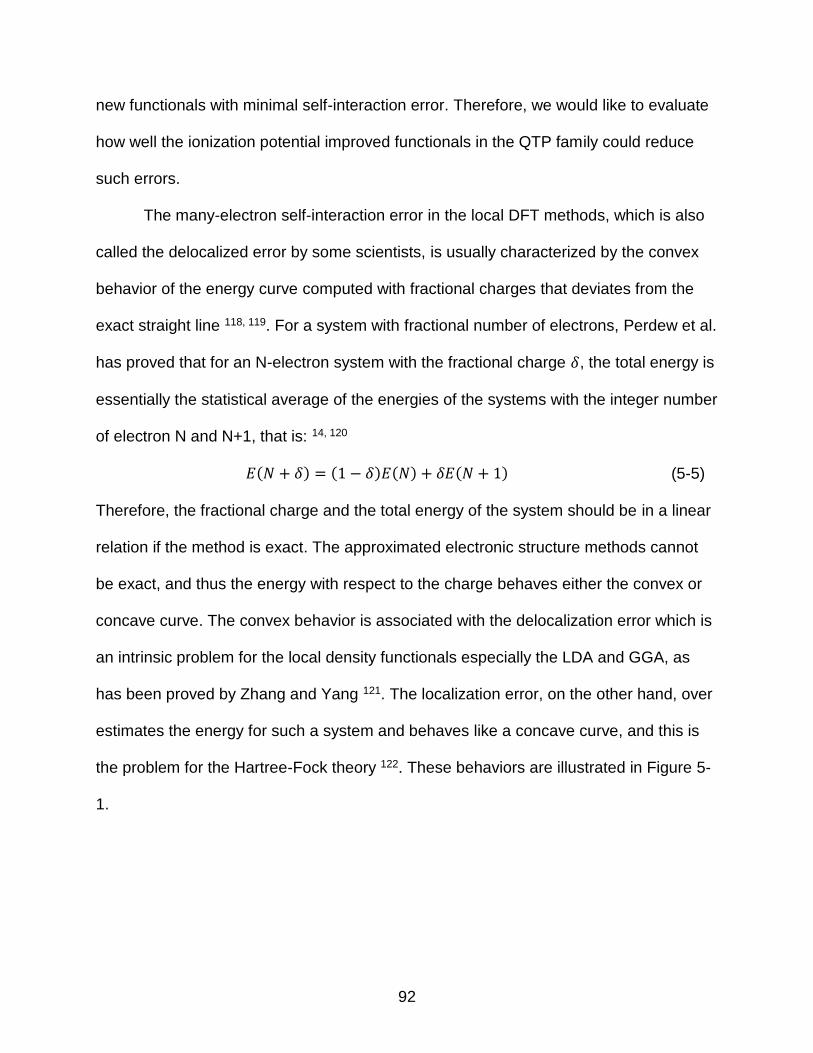
92

new functionals with minimal self-interaction error. Therefore, we would like to evaluate

how well the ionization potential improved functionals in the QTP family could reduce

such errors.

The many-electron self-interaction error in the local DFT methods, which is also

called the delocalized error by some scientists, is usually characterized by the convex

behavior of the energy curve computed with fractional charges that deviates from the

exact straight line 118, 119. For a system with fractional number of electrons, Perdew et al.

has proved that for an N-electron system with the fractional charge 𝛿, the total energy is

essentially the statistical average of the energies of the systems with the integer number

of electron N and N+1, that is: 14, 120

𝐸(𝑁 + 𝛿) = (1 − 𝛿)𝐸(𝑁) + 𝛿𝐸(𝑁 + 1) (5-5)

Therefore, the fractional charge and the total energy of the system should be in a linear

relation if the method is exact. The approximated electronic structure methods cannot

be exact, and thus the energy with respect to the charge behaves either the convex or

concave curve. The convex behavior is associated with the delocalization error which is

an intrinsic problem for the local density functionals especially the LDA and GGA, as

has been proved by Zhang and Yang 121. The localization error, on the other hand, over

estimates the energy for such a system and behaves like a concave curve, and this is

the problem for the Hartree-Fock theory 122. These behaviors are illustrated in Figure 5-

1.

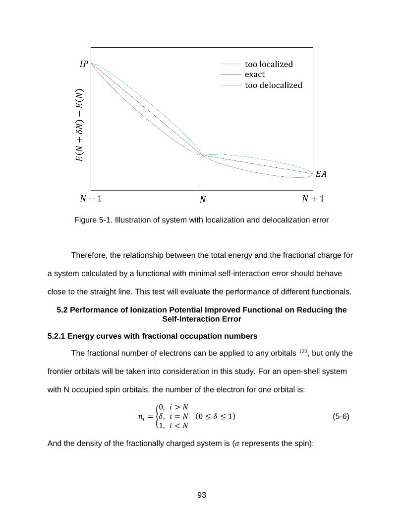
93

Figure 5-1. Illustration of system with localization and delocalization error

Therefore, the relationship between the total energy and the fractional charge for

a system calculated by a functional with minimal self-interaction error should behave

close to the straight line. This test will evaluate the performance of different functionals.

5.2 Performance of Ionization Potential Improved Functional on Reducing the Self-Interaction Error

5.2.1 Energy curves with fractional occupation numbers

The fractional number of electrons can be applied to any orbitals 123, but only the

frontier orbitals will be taken into consideration in this study. For an open-shell system

with N occupied spin orbitals, the number of the electron for one orbital is:

𝑛𝑖 = {0, 𝑖 > 𝑁𝛿, 𝑖 = 𝑁1, 𝑖 < 𝑁

(0 ≤ 𝛿 ≤ 1) (5-6)

And the density of the fractionally charged system is (𝜎 represents the spin):

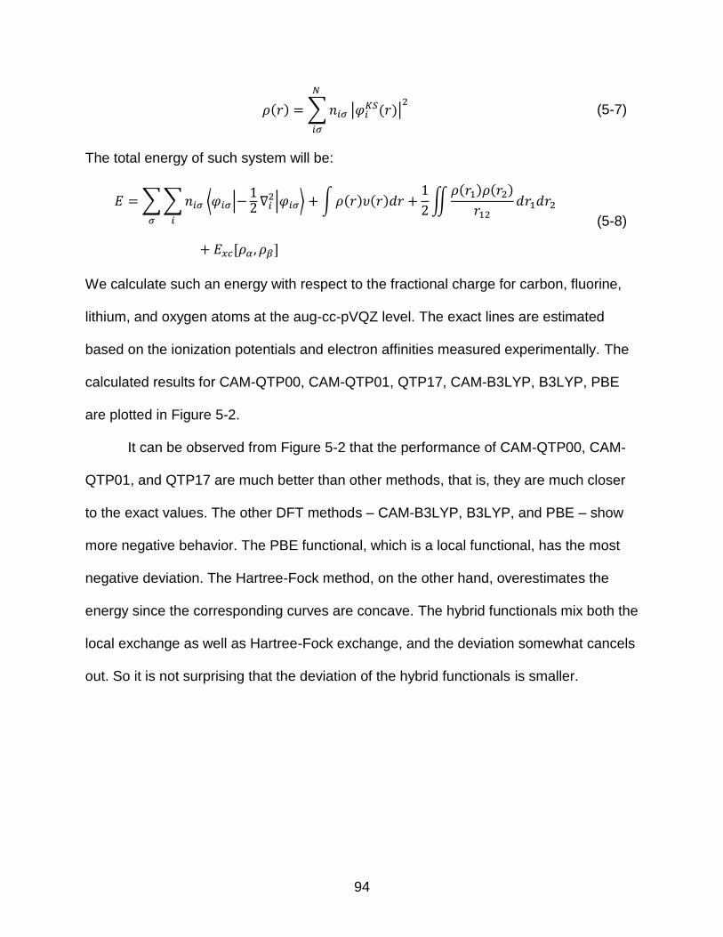
94

𝜌(𝑟) = ∑ 𝑛𝑖𝜎

𝑁

𝑖𝜎

|𝜑𝑖𝐾𝑆(𝑟)|

2 (5-7)

The total energy of such system will be:

𝐸 = ∑ ∑ 𝑛𝑖𝜎 ⟨𝜑𝑖𝜎|−12 ∇𝑖

2|𝜑𝑖𝜎⟩ + ∫ 𝜌(𝑟)𝜐(𝑟)𝑑𝑟 +1

2∬


𝑟12𝑑𝑟1𝑑𝑟2

𝑖𝜎

+ 𝐸𝑥𝑐[𝜌𝛼 , 𝜌𝛽]

(5-8)

We calculate such an energy with respect to the fractional charge for carbon, fluorine,

lithium, and oxygen atoms at the aug-cc-pVQZ level. The exact lines are estimated

based on the ionization potentials and electron affinities measured experimentally. The

calculated results for CAM-QTP00, CAM-QTP01, QTP17, CAM-B3LYP, B3LYP, PBE

are plotted in Figure 5-2.

It can be observed from Figure 5-2 that the performance of CAM-QTP00, CAM-

QTP01, and QTP17 are much better than other methods, that is, they are much closer

to the exact values. The other DFT methods – CAM-B3LYP, B3LYP, and PBE – show

more negative behavior. The PBE functional, which is a local functional, has the most

negative deviation. The Hartree-Fock method, on the other hand, overestimates the

energy since the corresponding curves are concave. The hybrid functionals mix both the

local exchange as well as Hartree-Fock exchange, and the deviation somewhat cancels

out. So it is not surprising that the deviation of the hybrid functionals is smaller.

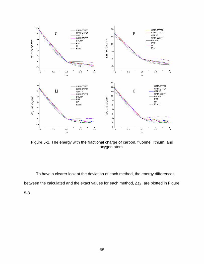
95

Figure 5-2. The energy with the fractional charge of carbon, fluorine, lithium, and oxygen atom

To have a clearer look at the deviation of each method, the energy differences

between the calculated and the exact values for each method, ∆𝐸𝑓, are plotted in Figure

5-3.

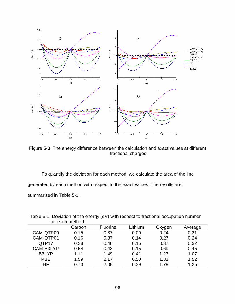
96

Figure 5-3. The energy difference between the calculation and exact values at different fractional charges

To quantify the deviation for each method, we calculate the area of the line

generated by each method with respect to the exact values. The results are


Table 5-1. Deviation of the energy (eV) with respect to fractional occupation number for each method

Carbon Fluorine Lithium Oxygen Average

CAM-QTP00 0.15 0.37 0.09 0.24 0.21 CAM-QTP01 0.16 0.37 0.14 0.27 0.24

QTP17 0.28 0.46 0.15 0.37 0.32 CAM-B3LYP 0.54 0.43 0.15 0.69 0.45

B3LYP 1.11 1.49 0.41 1.27 1.07 PBE 1.59 2.17 0.50 1.81 1.52 HF 0.73 2.08 0.39 1.79 1.25

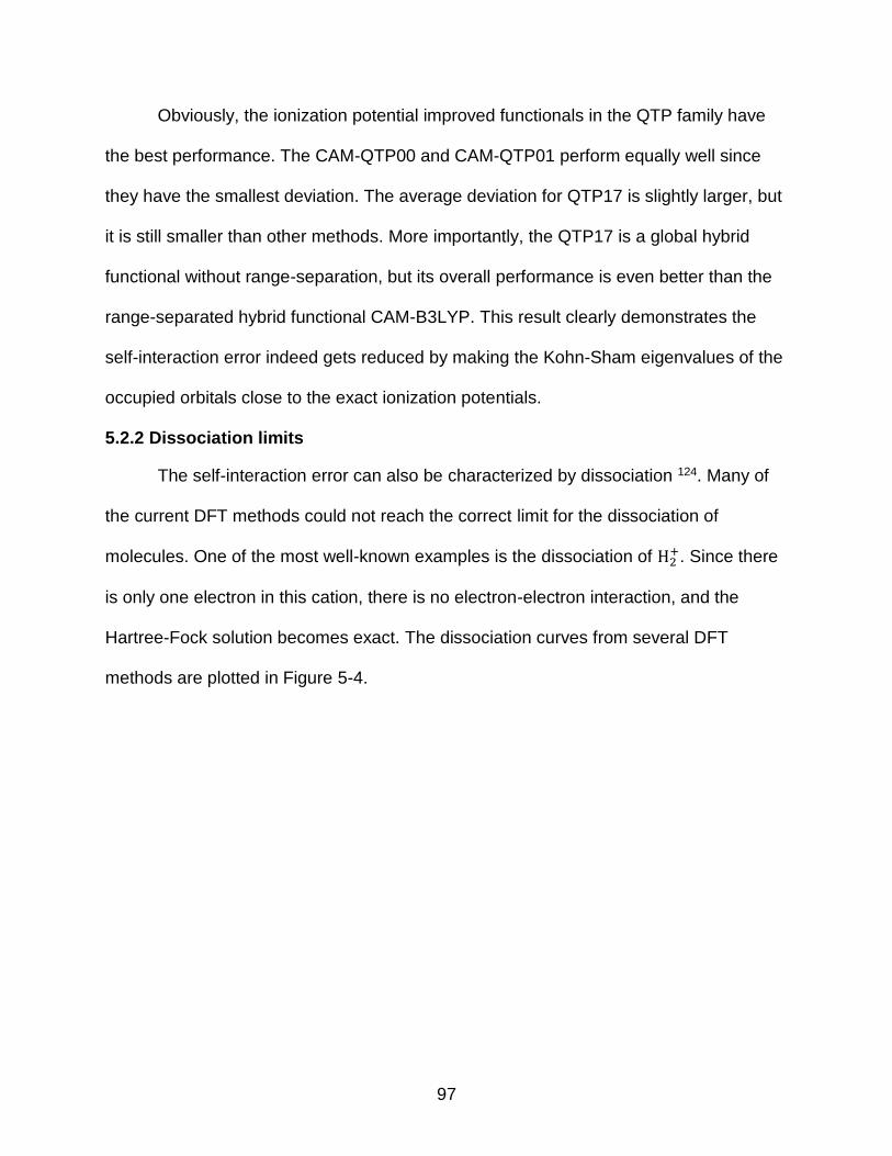
97

Obviously, the ionization potential improved functionals in the QTP family have

the best performance. The CAM-QTP00 and CAM-QTP01 perform equally well since

they have the smallest deviation. The average deviation for QTP17 is slightly larger, but

it is still smaller than other methods. More importantly, the QTP17 is a global hybrid

functional without range-separation, but its overall performance is even better than the

range-separated hybrid functional CAM-B3LYP. This result clearly demonstrates the

self-interaction error indeed gets reduced by making the Kohn-Sham eigenvalues of the

occupied orbitals close to the exact ionization potentials.

5.2.2 Dissociation limits

The self-interaction error can also be characterized by dissociation 124. Many of

the current DFT methods could not reach the correct limit for the dissociation of

molecules. One of the most well-known examples is the dissociation of H2+. Since there

is only one electron in this cation, there is no electron-electron interaction, and the

Hartree-Fock solution becomes exact. The dissociation curves from several DFT

methods are plotted in Figure 5-4.

98

Figure 5-4. Dissociation curve of H2+ cation

The energy of H2+ at the dissociation distance of 11 Å calculated at the Hartree-

Fock level is taken as the reference. Clearly, from Figure 5-4, the energy at the

dissociation limit computed by all the DFT methods are more or less underestimated

compared to the Hartree-Fock result. But overall, the curves computed by the three

ionization potential improved functionals, the CAM-QTP00, CAM-QTP01, and QTP17,

are closest to the exact curve. The errors at the dissociation limit of these three

functionals are 0.56 eV, 0.62 eV, and 0.67 eV respectively, much smaller than other

methods. It can also be noticed that the curves for B3LYP and PBE display a local

maximum which is not correct. The QTP17 correctly solves this problem.

99

The dissociation can also be represented by the variation of the fractional

charge. For a neutral molecule, as it dissociates into a cation and an anion, the charges

between them will first be somewhat delocalized and gradually localize onto the two

fragments. As has been shown in the previous section, the relationship between the

energy with respect to the fractional charge should be linear, and thus the dissociation

curve should also be a straight line if the method is exact. The curves for Li + F → Li+ +

F− is plotted in Figure 5-5.

Figure 5-5. The energy difference between Li+F and fractionally charged ions

Among all the methods tested, the CAM-QTP01 has the best performance. The

QTP17 does not reach the right limit, but it is close to the exact line. Again, the CAM-

QTP00, CAM-QTP01, and QTP17 perform much better than other DFT methods.

100

5.3 Conclusions

The self-interaction error is a fundamental problem for the standard DFT

methods, and it makes the functionals hard to converge to the right answer since the

exact one-particle theory should be self-interaction free. In this chapter, we have made

several self-interaction tests, and many standard functionals deviate greatly from the

exact behavior. The ionization potential improved functionals – CAM-QTP00, CAM-

QTP01, and QTP17 – have the best performance.

Noticeably, these three functionals in the QTP family do not take any properties

relate to the self-interaction as the training set when they are designed. They are just

ensured to make the orbitals energies close enough to the exact ionization potentials.

However, they not only perform well for many challenging properties in chemistry and

physics but significantly reduce the self-interaction error as well. Therefore, this chapter

further demonstrates the significance by enforcing the IP requirement for the Kohn-

Sham orbital energies. This requirement cannot be guaranteed to find the right

functional, but it finds a route for the functionals to converge to the right answer for the

right reason.

101

LIST OF REFERENCES

1. Szabo, A.; Ostlund, N. S., Modern Quantum Chemistry - Introduction to

Advanced Electronic Structure Theory. McGraw-Hill, Inc.: New York, 1982.

2. Parr, R. G.; Yang, W., Density Functional Theory of Atoms and Molecules. Oxford University Press: Oxford, 1989.

3. Shavitt, I.; Bartlett, R. J., Many‑Body Methods in Chemistry and Physics: MBPT

and Coupled‑Cluster Theory. Cambridge University Press: Cambridge, 2009.

4. Lyakh, D. I.; Musiał, M.; Lotrich, V. F.; Bartlett, R. J., Multireference Nature of Chemistry: The Coupled-Cluster View. Chem. Rev. 2011, 112 (1), 182-243.

5. Bartlett, R. J.; Silver, D. M., Many-body perturbation theory applied to electron pair correlation energies. I. Closed-shell first-row diatomic hydrides. J. Chem. Phys. 1975, 62 (8), 3258-3268.

6. Purvis, G. D.; Bartlett, R. J., A full coupled-cluster singles and doubles model: The inclusion of disconnected triples. J. Chem. Phys. 1982, 76 (4), 1910.

7. Urban, M.; Noga, J.; Cole, S. J.; Bartlett, R. J., Towards a full CCSDT model for electron correlation. J. Chem. Phys. 1985, 83 (8), 4041-4046.

8. Salter, E. A.; Trucks, G. W.; Bartlett, R. J., Analytic energy derivatives in many-body methods. I. First derivatives. J. Chem. Phys. 1989, 90 (3), 1752-1766.

9. Gauss, J.; Stanton, J. F.; Bartlett, R. J., Coupled-cluster open-shell analytic gradients: Implementation of the direct product decomposition approach in energy gradient calculations. J. Chem. Phys. 1991, 95 (4), 2623-2638.

10. Watts, J. D.; Gauss, J.; Bartlett, R. J., Coupled-cluster methods with noniterative triple excitations for restricted open-shell Hartree--Fock and other general single determinant reference functions. Energies and analytical gradients. J. Chem. Phys. 1993, 98 (11), 8718-8733.

11. Bartlett, R. J., The coupled-cluster revolution. Mol. Phys. 2010, 108 (21-23), 2905-2920.

12. Silver, D. M.; Bartlett, R. J., Modified potentials in many-body perturbation theory. Phys. Rev. A 1976, 13 (1), 1-12.

13. Bartlett, R.; Musiał, M., Coupled-cluster theory in quantum chemistry. Rev. Mod. Phys. 2007, 79 (1), 291-352.

14. Cohen, A. J.; Mori-Sánchez, P.; Yang, W., Challenges for Density Functional Theory. Chem. Rev. 2012, 112 (1), 289-320.

102

15. Geerlings, P.; De Proft, F.; Langenaeker, W., Conceptual Density Functional Theory. Chem. Rev. 2003, 103 (5), 1793-1874.

16. Jones, R. O., Density functional theory: Its origins, rise to prominence, and future. Rev. Mod. Phys. 2015, 87 (3), 897-923.

17. Kohn, W., Nobel Lecture: Electronic structure of matter—wave functions and density functionals. Rev. Mod. Phys. 1999, 71 (5), 1253-1266.

18. Ziegler, T., Approximate density functional theory as a practical tool in molecular energetics and dynamics. Chem. Rev. 1991, 91 (5), 651-667.

19. Kohn, W.; Sham, L. J., Self-Consistent Equations Including Exchange and Correlation Effects. Phys. Rev. 1965, 140 (4A), A1133-A1138.

20. Perdew, J. P.; Schmidt, K.; Van Doren, V.; Van Alsenoy, C.; Geerlings, P., Jacob’s ladder of density functional approximations for the exchange-correlation energy. AIP Conference Proceedings 2001, 577 (1), 1-20.

21. Mosquera, M. A.; Borca, C. H.; Ratner, M. A.; Schatz, G. C., Connection between Hybrid Functionals and Importance of the Local Density Approximation. J. Phys. Chem. A 2016, 120 (9), 1605-1612.

22. Vosko, S. H.; Wilk, L.; Nusair, M., Accurate spin-dependent electron liquid correlation energies for local spin density calculations: a critical analysis. Can. J. Phys. 1980, 58 (8), 1200-1211.

23. Gunnarsson, O.; Lundqvist, B. I., Exchange and correlation in atoms, molecules, and solids by the spin-density-functional formalism. Phys. Rev. B 1976, 13 (10), 4274-4298.

24. Perdew, J. P.; Zunger, A., Self-interaction correction to density-functional approximations for many-electron systems. Phys. Rev. B 1981, 23 (10), 5048-5079.

25. Becke, A. D., Density-functional exchange-energy approximation with correct asymptotic behavior. Phys. Rev. A 1988, 38 (6), 3098-3100.

26. Langreth, D. C.; Mehl, M. J., Beyond the local-density approximation in calculations of ground-state electronic properties. Phys. Rev. B 1983, 28 (4), 1809-1834.

27. Lee, C.; Yang, W.; Parr, R. G., Development of the Colle-Salvetti correlation-energy formula into a functional of the electron density. Phys. Rev. B 1988, 37 (2), 785-789.

28. Perdew, J. P.; Burke, K.; Ernzerhof, M., Generalized Gradient Approximation Made Simple. Phys. Rev. Lett. 1996, 77 (18), 3865-3868.

103

29. Adamo, C.; Barone, V., Toward reliable density functional methods without adjustable parameters: The PBE0 model. J. Chem. Phys. 1999, 110 (13), 6158-6170.

30. Stephens, P. J.; Devlin, F. J.; Chabalowski, C. F.; Frisch, M. J., Ab Initio Calculation of Vibrational Absorption and Circular Dichroism Spectra Using Density Functional Force Fields. J. Phys. Chem. 1994, 98 (45), 11623-11627.

31. Zhao, Y.; Truhlar, D. G., Density Functional for Spectroscopy: No Long-Range Self-Interaction Error, Good Performance for Rydberg and Charge-Transfer States, and Better Performance on Average than B3LYP for Ground States. J. Phys. Chem. A 2006, 110 (49), 13126-13130.

32. Becke, A. D., Density‐functional thermochemistry. III. The role of exact

exchange. J. Chem. Phys. 1993, 98 (7), 5648-5652.

33. Kohn, W.; Becke, A. D.; Parr, R. G., Density Functional Theory of Electronic Structure. J. Phys. Chem. 1996, 100 (31), 12974-12980.

34. Perdew, J. P., Size-Consistency, Self-Interaction Correction, and Derivative Discontinuity in Density Functional Theory. In Adv. Quantum Chem., Per-Olov, L., Ed. Academic Press: 1990; Vol. Volume 21, pp 113-134.

35. Bartlett, R. J., Coupled-cluster theory and its equation-of-motion extensions. Wiley Interdiscip. Rev.-Comput. Mol. Sci. 2012, 2 (1), 126-138.

36. Comeau, D. C.; Bartlett, R. J., The equation-of-motion coupled-cluster method. Applications to open- and closed-shell reference states. Chemical Physics Letters 1993, 207 (4–6), 414-423.

37. Del Bene, J. E.; Watts, J. D.; Bartlett, R. J., Coupled-cluster calculations of the excitation energies of benzene and the azabenzenes. J. Chem. Phys. 1997, 106 (14), 6051-6060.

38. Stanton, J. F.; Bartlett, R. J., The equation of motion coupled-cluster method. A systematic biorthogonal approach to molecular excitation energies, transition probabilities, and excited state properties. J. Chem. Phys. 1993, 98 (9), 7029-7039.

39. Watts, J. D.; Bartlett, R. J., The inclusion of connected triple excitations in the equation-of-motion coupled-cluster method. J. Chem. Phys. 1994, 101 (4), 3073-3078.

40. Bartlett, R. J., Towards an exact correlated orbital theory for electrons. Chem. Phys. Lett. 2009, 484 (1–3), 1-9.

41. Bartlett, R. J., Ab initioDFT and its role in electronic structure theory. Mol. Phys. 2010, 108 (21-23), 3299-3311.

104

42. Bartlett, R. J.; Lotrich, V. F.; Schweigert, I. V., Ab initio density functional theory: The best of both worlds? J. Chem. Phys. 2005, 123 (6), 062205.

43. Schweigert, I. V.; Bartlett, R. J., Effect of the nonlocal exchange on the performance of the orbital-dependent correlation functionals from second-order perturbation theory. J. Chem. Phys. 2008, 129 (12), 124109.

44. Talman, J. D.; Shadwick, W. F., Optimized effective atomic central potential. Phys. Rev. A 1976, 14 (1), 36-40.

45. Verma, P.; Bartlett, R. J., Increasing the applicability of density functional theory. III. Do consistent Kohn-Sham density functional methods exist? J. Chem. Phys. 2012, 137 (13), 134102.

46. Verma, P.; Bartlett, R. J., Increasing the applicability of density functional theory. II. Correlation potentials from the random phase approximation and beyond. J. Chem. Phys. 2012, 136 (4), 044105.

47. Chong, D. P.; Gritsenko, O. V.; Baerends, E. J., Interpretation of the Kohn-Sham orbital energies as approximate vertical ionization potentials. J. Chem. Phys. 2002, 116 (5), 1760-1772.

48. NIST Computational Chemistry Comparison and Benchmark Database , NIST Standard Reference Database Number 101, Release 17b, September 2015, Editor: Russell D. Johnson III , http://cccbdb.nist.gov/.

49. Stanton, J. F.; Gauss, J.; Watts, J. D.; Nooijen, M.; Oliphant, N.; Perera, S. A.; Szalay, P. G.; Lauderdale, W. J.; Kucharski, S. A.; Gwaltney, S. R.; Beck, S.; Balková, A.; Bernholdt, D. E.; Baeck, K. K.; Rozyczko, P.; Sekino, H.; Hober, C.; Bartlett, R. J. ACES II is a program product of the Quantum Theory Project, University of Florida. Integral packages included are VMOL (J. Almlöf and P. R. Taylor ); VPROPS (P. Taylor); ABACUS (T. Aa. Helgaker, H. J. Jensen, P. Jørgensen, J. Olsen and P. R. Taylor).

50. Valiev, M.; Bylaska, E. J.; Govind, N.; Kowalski, K.; Straatsma, T. P.; Van Dam, H. J. J.; Wang, D.; Nieplocha, J.; Apra, E.; Windus, T. L.; de Jong, W. A., NWChem: A comprehensive and scalable open-source solution for large scale molecular simulations. Comput. Phys. Commun. 2010, 181 (9), 1477-1489.

51. Yanai, T.; Tew, D. P.; Handy, N. C., A new hybrid exchange–correlation functional using the Coulomb-attenuating method (CAM-B3LYP). Chem. Phys. Lett. 2004, 393 (1–3), 51-57.

52. Zhao, Y.; Truhlar, D., The M06 suite of density functionals for main group thermochemistry, thermochemical kinetics, noncovalent interactions, excited states, and transition elements: two new functionals and systematic testing of four M06-class functionals and 12 other functionals. Theor. Chem. Account. 2008, 120 (1-3), 215-241.

http://cccbdb.nist.gov/

105

53. Grimme, S., Semiempirical hybrid density functional with perturbative second-order correlation. J. Chem. Phys. 2006, 124 (3), 034108.

54. Perdew, J. P., Density-functional approximation for the correlation energy of the inhomogeneous electron gas. Phys. Rev. B 1986, 33 (12), 8822-8824.

55. Perdew, J. P.; Chevary, J. A.; Vosko, S. H.; Jackson, K. A.; Pederson, M. R.; Singh, D. J.; Fiolhais, C., Atoms, molecules, solids, and surfaces: Applications of the generalized gradient approximation for exchange and correlation. Phys. Rev. B 1992, 46 (11), 6671-6687.

56. Livshits, E.; Baer, R., A well-tempered density functional theory of electrons in molecules. Phys. Chem. Chem. Phys. 2007, 9 (23), 2932-2941.

57. Tsuneda, T.; Suzumura, T.; Hirao, K., A new one-parameter progressive Colle–Salvetti-type correlation functional. J. Chem. Phys. 1999, 110 (22), 10664-10678.

58. Hamprecht, F. A.; Cohen, A. J.; Tozer, D. J.; Handy, N. C., Development and assessment of new exchange-correlation functionals. J. Chem. Phys. 1998, 109 (15), 6264-6271.

59. Boese, A. D.; Doltsinis, N. L.; Handy, N. C.; Sprik, M., New generalized gradient approximation functionals. J. Chem. Phys. 2000, 112 (4), 1670-1678.

60. Boese, A. D.; Handy, N. C., A new parametrization of exchange–correlation generalized gradient approximation functionals. J. Chem. Phys. 2001, 114 (13), 5497-5503.

61. Menconi, G.; Wilson, P. J.; Tozer, D. J., Emphasizing the exchange-correlation potential in functional development. J. Chem. Phys. 2001, 114 (9), 3958-3967.

62. Heyd, J.; Scuseria, G. E.; Ernzerhof, M., Hybrid functionals based on a screened Coulomb potential. J. Chem. Phys. 2003, 118 (18), 8207-8215.

63. Krukau, A. V.; Vydrov, O. A.; Izmaylov, A. F.; Scuseria, G. E., Influence of the exchange screening parameter on the performance of screened hybrid functionals. J. Chem. Phys. 2006, 125 (22), 224106.

64. Lange, A. W.; Rohrdanz, M. A.; Herbert, J. M., Charge-Transfer Excited States in a π-Stacked Adenine Dimer, As Predicted Using Long-Range-Corrected Time-Dependent Density Functional Theory. J. Phys. Chem. B 2008, 112 (20), 6304-6308.

65. Vydrov, O. A.; Scuseria, G. E., Assessment of a long-range corrected hybrid functional. J. Chem. Phys. 2006, 125 (23), 234109.

106

66. Izmaylov, A. F.; Scuseria, G. E.; Frisch, M. J., Efficient evaluation of short-range Hartree-Fock exchange in large molecules and periodic systems. J. Chem. Phys. 2006, 125 (10), 104103.

67. Zhao, Y.; Schultz, N. E.; Truhlar, D. G., Exchange-correlation functional with broad accuracy for metallic and nonmetallic compounds, kinetics, and noncovalent interactions. J. Chem. Phys. 2005, 123 (16), 161103.

68. Zhao, Y.; Schultz, N. E.; Truhlar, D. G., Design of Density Functionals by Combining the Method of Constraint Satisfaction with Parametrization for Thermochemistry, Thermochemical Kinetics, and Noncovalent Interactions. J. Chem. Theory Comput. 2006, 2 (2), 364-382.

69. Zhao, Y.; Truhlar, D. G., A new local density functional for main-group thermochemistry, transition metal bonding, thermochemical kinetics, and noncovalent interactions. J. Chem. Phys. 2006, 125 (19), 194101.

70. Zhao, Y.; Truhlar, D. G., Exploring the Limit of Accuracy of the Global Hybrid Meta Density Functional for Main-Group Thermochemistry, Kinetics, and Noncovalent Interactions. J. Chem. Theory Comput. 2008, 4 (11), 1849-1868.

71. Peverati, R.; Truhlar, D. G., Improving the Accuracy of Hybrid Meta-GGA Density Functionals by Range Separation. J. Phys. Chem. Lett. 2011, 2 (21), 2810-2817.

72. Peverati, R.; Truhlar, D. G., M11-L: A Local Density Functional That Provides Improved Accuracy for Electronic Structure Calculations in Chemistry and Physics. J. Phys. Chem. Lett. 2012, 3 (1), 117-124.

73. Lynch, B. J.; Fast, P. L.; Harris, M.; Truhlar, D. G., Adiabatic Connection for Kinetics. J. Phys. Chem. A 2000, 104 (21), 4811-4815.

74. Tsuneda, T.; Suzumura, T.; Hirao, K., A reexamination of exchange energy functionals. J. Chem. Phys. 1999, 111 (13), 5656-5667.

75. Cohen, A. J.; Mori-Sánchez, P.; Yang, W., Development of exchange-correlation functionals with minimal many-electron self-interaction error. J. Chem. Phys. 2007, 126 (19), 191109.

76. Zhao, Y.; Truhlar, D. G., Construction of a generalized gradient approximation by restoring the density-gradient expansion and enforcing a tight Lieb–Oxford bound. J. Chem. Phys. 2008, 128 (18), 184109.

77. Peverati, R.; Zhao, Y.; Truhlar, D. G., Generalized Gradient Approximation That Recovers the Second-Order Density-Gradient Expansion with Optimized Across-the-Board Performance. J. Phys. Chem. Lett. 2011, 2 (16), 1991-1997.

107

78. Fransson, T.; Harada, Y.; Kosugi, N.; Besley, N. A.; Winter, B.; Rehr, J. J.; Pettersson, L. G. M.; Nilsson, A., X-ray and Electron Spectroscopy of Water. Chem. Rev. 2016, 116 (13), 7551-7569.

79. Jolly, W. L.; Bomben, K. D.; Eyermann, C. J., Core-electron binding energies for gaseous atoms and molecules. At. Data Nucl. Data Tables 1984, 31 (3), 433-493.

80. Verma, P.; Bartlett, R. J., Increasing the applicability of density functional theory. IV. Consequences of ionization-potential improved exchange-correlation potentials. J. Chem. Phys. 2014, 140 (18), 18A534.

81. Yu, H. S.; He, X.; Li, S. L.; Truhlar, D. G., MN15: A Kohn-Sham global-hybrid exchange-correlation density functional with broad accuracy for multi-reference and single-reference systems and noncovalent interactions. Chem. Sci. 2016, 7 (8), 5032-5051.

82. Zhang, Y.; Mukamel, S.; Khalil, M.; Govind, N., Simulating Valence-to-Core X-ray Emission Spectroscopy of Transition Metal Complexes with Time-Dependent Density Functional Theory. J. Chem. Theory Comput. 2015, 11 (12), 5804-5809.

83. Lopata, K.; Van Kuiken, B. E.; Khalil, M.; Govind, N., Linear-Response and Real-Time Time-Dependent Density Functional Theory Studies of Core-Level Near-Edge X-Ray Absorption. J. Chem. Theory Comput. 2012, 8 (9), 3284-3292.

84. Verma, P.; Bartlett, R. J., Increasing the applicability of density functional theory. V. X-ray absorption spectra with ionization potential corrected exchange and correlation potentials. J. Chem. Phys. 2016, 145 (3), 034108.

85. Jin, Y.; Bartlett, R. J., The QTP family of consistent functionals and potentials in Kohn-Sham density functional theory. J. Chem. Phys. 2016, 145 (3), 034107.

86. Maitra, N. T., Perspective: Fundamental aspects of time-dependent density functional theory. J. Chem. Phys. 2016, 144 (22), 220901.

87. Bartlett, R. J.; Ranasinghe, D. S., The power of exact conditions in electronic structure theory. Chem. Phys. Lett. 2017, 669, 54-70.

88. Hirao, K.; Nakatsuji, H., A generalization of the Davidson's method to large nonsymmetric eigenvalue problems. J. Comput. Phys. 1982, 45 (2), 246-254.

89. Besley, N. A.; Peach, M. J. G.; Tozer, D. J., Time-dependent density functional theory calculations of near-edge X-ray absorption fine structure with short-range corrected functionals. Phys. Chem. Chem. Phys. 2009, 11 (44), 10350-10358.

90. Bandyopadhyay, P.; Segre, C. U. http://www.csrri.iit.edu/mucal.html.

http://www.csrri.iit.edu/mucal.html

108

91. Dreuw, A.; Weisman, J. L.; Head-Gordon, M., Long-range charge-transfer excited states in time-dependent density functional theory require non-local exchange. J. Chem. Phys. 2003, 119 (6), 2943-2946.

92. Moore, B.; Sun, H.; Govind, N.; Kowalski, K.; Autschbach, J., Charge-Transfer Versus Charge-Transfer-Like Excitations Revisited. J. Chem. Theory Comput. 2015, 11 (7), 3305-3320.

93. Isegawa, M.; Peverati, R.; Truhlar, D. G., Performance of recent and high-performance approximate density functionals for time-dependent density functional theory calculations of valence and Rydberg electronic transition energies. J. Chem. Phys. 2012, 137 (24), 244104.

94. Caricato, M.; Trucks, G. W.; Frisch, M. J.; Wiberg, K. B., Electronic Transition Energies: A Study of the Performance of a Large Range of Single Reference Density Functional and Wave Function Methods on Valence and Rydberg States Compared to Experiment. J. Chem. Theory Comput. 2010, 6 (2), 370-383.

95. Grimme, S.; Neese, F., Double-hybrid density functional theory for excited electronic states of molecules. J. Chem. Phys. 2007, 127 (15), 154116.

96. Rohrdanz, M. A.; Martins, K. M.; Herbert, J. M., A long-range-corrected density functional that performs well for both ground-state properties and time-dependent density functional theory excitation energies, including charge-transfer excited states. J. Chem. Phys. 2009, 130 (5), 054112.

97. Tozer, D. J.; Handy, N. C., Improving virtual Kohn–Sham orbitals and eigenvalues: Application to excitation energies and static polarizabilities. J. Chem. Phys. 1998, 109 (23), 10180-10189.

98. Gill, P. M. W.; Adamson, R. D.; Pople, J. A., Coulomb-attenuated exchange energy density functionals. Mol. Phys. 1996, 88 (4), 1005-1009.

99. Iikura, H.; Tsuneda, T.; Yanai, T.; Hirao, K., A long-range correction scheme for generalized-gradient-approximation exchange functionals. J. Chem. Phys. 2001, 115 (8), 3540-3544.

100. Peach, M. J. G.; Helgaker, T.; Salek, P.; Keal, T. W.; Lutnaes, O. B.; Tozer, D. J.; Handy, N. C., Assessment of a Coulomb-attenuated exchange-correlation energy functional. Phys. Chem. Chem. Phys. 2006, 8 (5), 558-562.

101. Tawada, Y.; Tsuneda, T.; Yanagisawa, S.; Yanai, T.; Hirao, K., A long-range-corrected time-dependent density functional theory. J. Chem. Phys. 2004, 120 (18), 8425-8433.

102. Baer, R.; Neuhauser, D., Density Functional Theory with Correct Long-Range Asymptotic Behavior. Phys. Rev. Lett. 2005, 94 (4), 043002.

109

103. Mardirossian, N.; Head-Gordon, M., ωB97X-V: A 10-parameter, range-separated hybrid, generalized gradient approximation density functional with nonlocal correlation, designed by a survival-of-the-fittest strategy. Phys. Chem. Chem. Phys. 2014, 16 (21), 9904-9924.

104. Curtiss, L. A.; Raghavachari, K.; Trucks, G. W.; Pople, J. A., Gaussian-2 theory

for molecular energies of first‐ and second‐row compounds. J. Chem. Phys.

1991, 94 (11), 7221-7230.

105. Goerigk, L.; Grimme, S., Assessment of TD-DFT methods and of various spin scaled CIS(D) and CC2 versions for the treatment of low-lying valence excitations of large organic dyes. J. Chem. Phys. 2010, 132 (18), 184103.

106. Goerigk, L.; Moellmann, J.; Grimme, S., Computation of accurate excitation energies for large organic molecules with double-hybrid density functionals. Phys. Chem. Chem. Phys. 2009, 11 (22), 4611-4620.

107. Weigend, F.; Ahlrichs, R., Balanced basis sets of split valence, triple zeta valence and quadruple zeta valence quality for H to Rn: Design and assessment of accuracy. Phys. Chem. Chem. Phys. 2005, 7 (18), 3297-3305.

108. Stein, T.; Kronik, L.; Baer, R., Reliable Prediction of Charge Transfer Excitations in Molecular Complexes Using Time-Dependent Density Functional Theory. J. Am. Chem. Soc 2009, 131 (8), 2818-2820.

109. Pople, J. A.; Head-Gordon, M.; Fox, D. J.; Raghavachari, K.; Curtiss, L. A., Gaussian-1 theory: A general procedure for prediction of molecular energies. J. Chem. Phys. 1989, 90 (10), 5622-5629.

110. Curtiss, L. A.; Raghavachari, K.; Redfern, P. C.; Pople, J. A., Assessment of Gaussian-2 and density functional theories for the computation of enthalpies of formation. J. Chem. Phys. 1997, 106 (3), 1063-1079.

111. Zipse, H., Radical Stability—A Theoretical Perspective. In Radicals in Synthesis I, Gansäuer, A., Ed. Springer Berlin Heidelberg: Berlin, Heidelberg, 2006; pp 163-189.

112. Soydaş, E.; Bozkaya, U., Assessment of Orbital-Optimized Third-Order Møller–Plesset Perturbation Theory and Its Spin-Component and Spin-Opposite Scaled Variants for Thermochemistry and Kinetics. J. Chem. Theory Comput. 2013, 9 (3), 1452-1460.

113. Copan, A. V.; Sokolov, A. Y.; Schaefer, H. F., Benchmark Study of Density Cumulant Functional Theory: Thermochemistry and Kinetics. J. Chem. Theory Comput. 2014, 10 (6), 2389-2398.

110

114. Lynch, B. J.; Truhlar, D. G., How Well Can Hybrid Density Functional Methods Predict Transition State Geometries and Barrier Heights? J. Phys. Chem. A 2001, 105 (13), 2936-2941.

115. Zhao, Y.; González-García, N.; Truhlar, D. G., Benchmark Database of Barrier Heights for Heavy Atom Transfer, Nucleophilic Substitution, Association, and Unimolecular Reactions and Its Use to Test Theoretical Methods. J. Phys. Chem. A 2005, 109 (9), 2012-2018.

116. Bokhan, D.; Bartlett, R. J., Adiabatic ab initio time-dependent density-functional theory employing optimized-effective-potential many-body perturbation theory potentials. Phys. Rev. A 2006, 73 (2), 022502.

117. Grabowski, I.; Hirata, S.; Ivanov, S.; Bartlett, R. J., Ab initio density functional theory: OEP-MBPT(2). A new orbital-dependent correlation functional. J. Chem. Phys. 2002, 116 (11), 4415-4425.

118. Haunschild, R.; Henderson, T. M.; Jiménez-Hoyos, C. A.; Scuseria, G. E., Many-electron self-interaction and spin polarization errors in local hybrid density functionals. J. Chem. Phys. 2010, 133 (13), 134116.

119. Cohen, A. J.; Mori-Sánchez, P.; Yang, W., Insights into Current Limitations of Density Functional Theory. Science 2008, 321 (5890), 792.

120. Perdew, J. P.; Parr, R. G.; Levy, M.; Balduz, J. L., Density-Functional Theory for Fractional Particle Number: Derivative Discontinuities of the Energy. Phys. Rev. Lett. 1982, 49 (23), 1691-1694.

121. Zhang, Y.; Yang, W., A challenge for density functionals: Self-interaction error increases for systems with a noninteger number of electrons. J. Chem. Phys. 1998, 109 (7), 2604-2608.

122. Li, C.; Yang, W., On the piecewise convex or concave nature of ground state energy as a function of fractional number of electrons for approximate density functionals. J. Chem. Phys. 2017, 146 (7), 074107.

123. Ranasinghe, D. S.; Margraf, J. T.; Jin, Y.; Bartlett, R. J., Does the ionization potential condition employed in QTP functionals mitigate the self-interaction error? J. Chem. Phys. 2017, 146 (3), 034102.

124. Gräfenstein, J.; Kraka, E.; Cremer, D., The impact of the self-interaction error on the density functional theory description of dissociating radical cations: Ionic and covalent dissociation limits. J. Chem. Phys. 2003, 120 (2), 524-539.

111

BIOGRAPHICAL SKETCH

Yifan grew up in a relatively big city, where he completed his high school and

undergraduate education. When he was still in the kindergarten, he already determined

to receive the doctoral degree in the future. Later, he was not reconciled to be a

common person; instead, he wanted to become extraordinary and be well known

around the world. The life was hard, but he never gave up. In the middle school, he felt

in love with chemistry. And when he was 19 years old, he changed his name to “Yifan”

based on the pronunciation of two chemical elements.

After he had received his bachelor’s degree, he was admitted as a graduate

student at the same University. However, it was always his dream to receive the best

education in the world. Although he struggled for three years and failed many times, he

eventually received the offer of admission from the University of Florida in 2011. There

he joined the quantum theory project and worked on the electronic structure theory. He

was a good researcher, and he was also a good teacher; he loved scientific research,

and he also loved his students.

In 2017, he finally completed his Ph.D. program. However, this just means that

he has achieved his dream in the kindergarten. He has a lot of dreams, and he is even

not sure if he could turn some of them into reality in his life. However, he will try his best

and relentless to achieve his lofty goals, to make the advancement of the science

forever and ever.

Documents

IONIZATION POTENTIAL IMPROVED CONSISTENT DENSITY