Embed Size (px)
Citation preview

Reprinted and altered with the written permission of ASHRAE and for chapter distribution only.
The publication may not be reproduced without permission from ASHRAE RP Fundraising Staff. 404/636-8400 or [email protected]
1791 Tullie Circle, Atlanta GA 30329
Preface
What would the world look like without ASHRAE Research? Since its beginnings in 1919,
ASHRAE Research has grown and expanded to address the ever changing questions and topics facing both its members and the HVAC&R Industry and the world as a whole. The ASHRAE Handbook is constantly evolving to address these new challenges, fueled by the knowledge and principals developed through ASHRAE Research. As the focus of the industry has evolved from home refrigeration and food safety to improved indoor air quality to sustainability and energy efficiency, this four-volume series continues to be the cornerstone in every ASHRAE Member’s career.
The power behind ASHRAE Research and the four-volume Handbook comes directly from YOU: your financial support is the driving force behind every research project conducted world wide; your financial investment is an investment in the future of the HVAC&R industry; your donation to ASHRAE Research fills the more than 3,600 Handbook pages.
What would the ASHRAE Handbook look like without your support of ASHRAE Research? Take a look at just one chapter and imagine a world without this guidance from ASHRAE over the last 90 years.
Thank you for all your support
Research Promotion Committee
18.1
CHAPTER 18
NONRESIDENTIAL COOLING AND HEATING LOAD CALCULATIONS
Cooling Load Calculation Principles ...................................... 18.1Internal Heat Gains ................................................................. 18.3Infiltration and Moisture Migration
Heat Gains ....................................................................... 18.12Fenestration Heat Gain.......................................................... 18.14Heat Balance Method ............................................................ 18.14
Radiant Time Series (RTS) Method ........................................ 18.20Heating Load Calculations .................................................... 18.28System Heating and Cooling Load Effects ............................. 18.32Example Cooling and Heating Load Calculations ................ 18.35Previous Cooling Load Calculation Methods ........................ 18.49Building Example Drawings .................................................. 18.52
EATING and cooling load calculations are the primary designHbasis for most heating and air-conditioning systems and com-ponents. These calculations affect the size of piping, ductwork, dif-fusers, air handlers, boilers, chillers, coils, compressors, fans, andevery other component of systems that condition indoor environ-ments. Cooling and heating load calculations can significantly affectfirst cost of building construction, comfort and productivity of occu-pants, and operating cost and energy consumption.
Simply put, heating and cooling loads are the rates of energyinput (heating) or removal (cooling) required to maintain an indoorenvironment at a desired temperature and humidity condition. Heat-ing and air conditioning systems are designed, sized, and controlledto accomplish that energy transfer. The amount of heating or coolingrequired at any particular time varies widely, depending on external(e.g., outdoor temperature) and internal (e.g., number of peopleoccupying a space) factors.
Peak design heating and cooling load calculations, which are thischapter’s focus, seek to determine the maximum rate of heating andcooling energy transfer needed at any point in time. Similar princi-ples, but with different assumptions, data, and application, can beused to estimate building energy consumption, as described in Chap-ter 19.
This chapter discusses common elements of cooling load calcu-lation (e.g., internal heat gain, ventilation and infiltration, moisturemigration, fenestration heat gain) and two methods of heating andcooling load estimation: heat balance (HB) and radiant time series(RTS).
COOLING LOAD CALCULATION PRINCIPLES
Cooling loads result from many conduction, convection, and radi-ation heat transfer processes through the building envelope and frominternal sources and system components. Building components orcontents that may affect cooling loads include the following:
• External: Walls, roofs, windows, skylights, doors, partitions, ceil-ings, and floors
• Internal: Lights, people, appliances, and equipment• Infiltration: Air leakage and moisture migration• System: Outdoor air, duct leakage and heat gain, reheat, fan and
pump energy, and energy recovery
TERMINOLOGY
The variables affecting cooling load calculations are numerous,often difficult to define precisely, and always intricately interrelated.
Many cooling load components vary widely in magnitude, and pos-sibly direction, during a 24 h period. Because these cyclic changes inload components often are not in phase with each other, each compo-nent must be analyzed to establish the maximum cooling load for abuilding or zone. A zoned system (i.e., one serving several indepen-dent areas, each with its own temperature control) needs to provide nogreater total cooling load capacity than the largest hourly sum ofsimultaneous zone loads throughout a design day; however, it musthandle the peak cooling load for each zone at its individual peak hour.At some times of day during heating or intermediate seasons, somezones may require heating while others require cooling. The zones’ventilation, humidification, or dehumidification needs must also beconsidered.
Heat Flow RatesIn air-conditioning design, the following four related heat flow
rates, each of which varies with time, must be differentiated.Space Heat Gain. This instantaneous rate of heat gain is the rate
at which heat enters into and/or is generated within a space. Heat gainis classified by its mode of entry into the space and whether it is sen-sible or latent. Entry modes include (1) solar radiation through trans-parent surfaces; (2) heat conduction through exterior walls and roofs;(3) heat conduction through ceilings, floors, and interior partitions;(4) heat generated in the space by occupants, lights, and appliances;(5) energy transfer through direct-with-space ventilation and infiltra-tion of outdoor air; and (6) miscellaneous heat gains. Sensible heat isadded directly to the conditioned space by conduction, convection,and/or radiation. Latent heat gain occurs when moisture is added tothe space (e.g., from vapor emitted by occupants and equipment). Tomaintain a constant humidity ratio, water vapor must condense on thecooling apparatus and be removed at the same rate it is added to thespace. The amount of energy required to offset latent heat gain essen-tially equals the product of the condensation rate and latent heat ofcondensation. In selecting cooling equipment, distinguish betweensensible and latent heat gain: every cooling apparatus has differentmaximum removal capacities for sensible versus latent heat for par-ticular operating conditions. In extremely dry climates, humidifica-tion may be required, rather than dehumidification, to maintainthermal comfort.
Radiant Heat Gain. Radiant energy must first be absorbed by sur-faces that enclose the space (walls, floor, and ceiling) and objects inthe space (furniture, etc.). When these surfaces and objects becomewarmer than the surrounding air, some of their heat transfers to the airby convection. The composite heat storage capacity of these surfacesand objects determines the rate at which their respective surfacetemperatures increase for a given radiant input, and thus governs therelationship between the radiant portion of heat gain and its corre-sponding part of the space cooling load (Figure 1). The thermal stor-age effect is critical in differentiating between instantaneous heatgain for a given space and its cooling load at that moment. Predicting
The preparation of this chapter is assigned to TC 4.1, Load Calculation Dataand Procedures.
primary designmost heating and air-conditioning systems and com-
ponents. size of piping, ductwork, dif-fusers, air handlers, boilers, chillers, coils, compressors, fans, andevery other component of systems that condition indoor environ-ments. n significantly affectfirst cost of building construction, comfort and productivity of occu-pants, and operating cost and energy consumption.t
rates of energyinput (heating) or removal (cooling) required to maintain an indoorenvironment at a desired temperature and humidity condition.
designed, sized, and controlledto accomplish that energy transfer. The amount of heating or coolingrequired at any particular time varies widely, depending on external(e.g., outdoor temperature) and internal (e.g., number of peopleoccupying a space) factors.
maximum rate of heating andcooling energy transfer needed at any point in time.
but with different assumptions, data, and application, can beused to estimate building energy consumption, a
common elements internal heat gain, ventilation and infiltration, moisture
migration, fenestration heat gain) two f heating andcooling load estimation: heat balance (HB) and radiant time series(RTS).
y conduction, convection, and radi-ation heat transfer processes through the building envelope and frominternal sources and system components.
t may affect cooling loads
Walls, roofs, windows, skylights, doors, partitions, ceil-ings, and floors
Lights, people, appliances, and equipment Air leakage and moisture migration
Outdoor air, duct leakage and heat gain, reheat, fan andpump energy, and energy recovery
numerous,n difficult to define precisely, d always intricately interrelated.
vary widely in magnitude, pos-sibly direction, during a 24 h period.load components often are not in phase with each other, each compo-nent must be analyzed to establish the maximum cooling load
o provide nogreater total cooling load capacity than the largest hourly sum ofsimultaneous zone loads throughout a design day; musthandle the peak cooling load for each zone at its individual peak hour.
f day during heating or intermediate seasons, somezones may require heating while others require cooling. The zones’ventilation, humidification, or dehumidification needs must also beconsidered.
differentiated.This instantaneous rate of heat gain is the rate
at which heat enters into and/or is generated within a space. Heat gainis classified by its mode of entry into the space and whether it is sen-sible or latent. E ) solar radiation through trans-parent surfaces; ( ) heat conduction through exterior walls and roofs;
heat conduction through ceilings, floors, and interior partitions;heat generated in the space by occupants, lights, and appliances;
energy transfer through direct-with-space ventilation and infiltra-tion of outdoor air; an o ) miscellaneous heat gains. isadded directly to the conditioned space by conduction, convection,and/or radiation. gain occurs when moisture is added tothe space (e.g., from vapor emitted by occupants and equipment). Tomaintain a constant humidity ratio, water vapor must condense on thecooling apparatus and be removed at the same rate it is added to thespace. The amount of energy required to offset latent heat gain essen-tially equals the product of the condensation rate and latent heat ofcondensation. In selecting cooling equipment, distinguish betweensensible and latent heat gain: every cooling apparatus has differentmaximum removal capacities for sensible versus latent heat for par-ticular operating conditions. In extremely dry climates, humidifica-tion may be required, rather than dehumidification, to maintainthermal comfort.
Radiant energy must first be absorbed by sur-faces that enclose the space (walls, floor, and ceiling) and objects inthe space (furniture, etc.).
determines the rate at which their respective surfacetemperatures increase for a given radiant input, and thus governs therelationship between the radiant portion of heat gain and its corre-rrsponding part of the space cooling load
critical in differentiating between instantaneous heatgain for a given space and its cooling load at that moment. P
18.2 2013 ASHRAE Handbook—Fundamentals
the nature and magnitude of this phenomenon to estimate a realisticcooling load for a particular set of circumstances has long been ofinterest to design engineers; the Bibliography lists some early workon the subject.
Space Cooling Load. This is the rate at which sensible and latentheat must be removed from the space to maintain a constant spaceair temperature and humidity. The sum of all space instantaneousheat gains at any given time does not necessarily (or even fre-quently) equal the cooling load for the space at that same time.
Space Heat Extraction Rate. The rates at which sensible andlatent heat are removed from the conditioned space equal the spacecooling load only if the room air temperature and humidity are con-stant. Along with the intermittent operation of cooling equipment,control systems usually allow a minor cyclic variation or swing inroom temperature; humidity is often allowed to float, but it can becontrolled. Therefore, proper simulation of the control system givesa more realistic value of energy removal over a fixed period thanusing values of the space cooling load. However, this is primarilyimportant for estimating energy use over time; it is not needed tocalculate design peak cooling load for equipment selection.
Cooling Coil Load. The rate at which energy is removed at acooling coil serving one or more conditioned spaces equals the sumof instantaneous space cooling loads (or space heat extraction rate,if it is assumed that space temperature and humidity vary) for allspaces served by the coil, plus any system loads. System loadsinclude fan heat gain, duct heat gain, and outdoor air heat and mois-ture brought into the cooling equipment to satisfy the ventilation airrequirement.
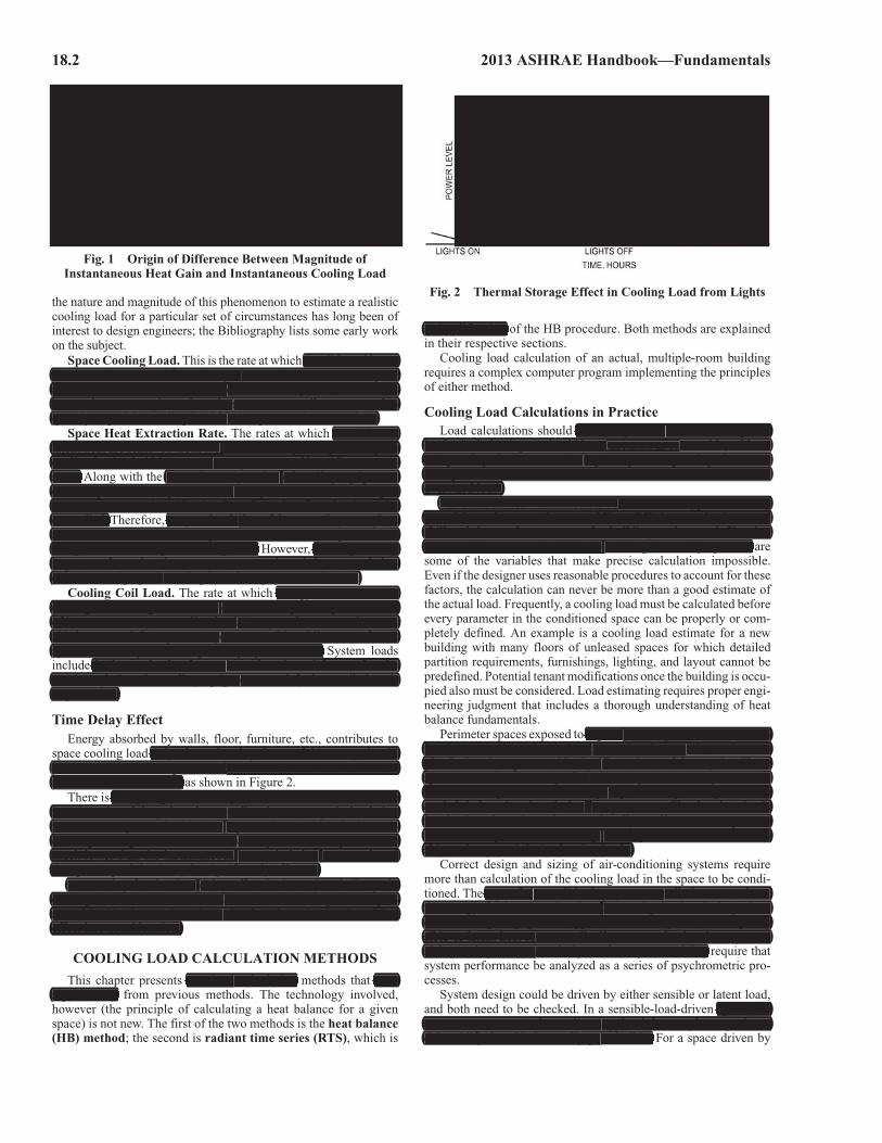
Time Delay EffectEnergy absorbed by walls, floor, furniture, etc., contributes to
space cooling load only after a time lag. Some of this energy is stillpresent and reradiating even after the heat sources have beenswitched off or removed, as shown in Figure 2.
There is always significant delay between the time a heat sourceis activated, and the point when reradiated energy equals that beinginstantaneously stored. This time lag must be considered when cal-culating cooling load, because the load required for the space can bemuch lower than the instantaneous heat gain being generated, andthe space’s peak load may be significantly affected.
Accounting for the time delay effect is the major challenge incooling load calculations. Several methods, including the two pre-sented in this chapter, have been developed to take the time delayeffect into consideration.
COOLING LOAD CALCULATION METHODS
This chapter presents two load calculation methods that varysignificantly from previous methods. The technology involved,however (the principle of calculating a heat balance for a givenspace) is not new. The first of the two methods is the heat balance(HB) method; the second is radiant time series (RTS), which is
a simplification of the HB procedure. Both methods are explainedin their respective sections.
Cooling load calculation of an actual, multiple-room buildingrequires a complex computer program implementing the principlesof either method.
Cooling Load Calculations in PracticeLoad calculations should accurately describe the building. All
load calculation inputs should be as accurate as reasonable, withoutusing safety factors. Introducing compounding safety factors atmultiple levels in the load calculation results in an unrealistic andoversized load.
Variation in heat transmission coefficients of typical buildingmaterials and composite assemblies, differing motivations andskills of those who construct the building, unknown infiltrationrates, and the manner in which the building is actually operated aresome of the variables that make precise calculation impossible.Even if the designer uses reasonable procedures to account for thesefactors, the calculation can never be more than a good estimate ofthe actual load. Frequently, a cooling load must be calculated beforeevery parameter in the conditioned space can be properly or com-pletely defined. An example is a cooling load estimate for a newbuilding with many floors of unleased spaces for which detailedpartition requirements, furnishings, lighting, and layout cannot bepredefined. Potential tenant modifications once the building is occu-pied also must be considered. Load estimating requires proper engi-neering judgment that includes a thorough understanding of heatbalance fundamentals.
Perimeter spaces exposed to high solar heat gain often need cool-ing during sunlit portions of traditional heating months, as do com-pletely interior spaces with significant internal heat gain. Thesespaces can also have significant heating loads during nonsunlithours or after periods of nonoccupancy, when adjacent spaces havecooled below interior design temperatures. The heating loadsinvolved can be estimated conventionally to offset or to compensatefor them and prevent overheating, but they have no direct relation-ship to the spaces’ design heating loads.
Correct design and sizing of air-conditioning systems requiremore than calculation of the cooling load in the space to be condi-tioned. The type of air-conditioning system, ventilation rate, reheat,fan energy, fan location, duct heat loss and gain, duct leakage, heatextraction lighting systems, type of return air system, and any sen-sible or latent heat recovery all affect system load and componentsizing. Adequate system design and component sizing require thatsystem performance be analyzed as a series of psychrometric pro-cesses.
System design could be driven by either sensible or latent load,and both need to be checked. In a sensible-load-driven space (themost common case), the cooling supply air has surplus capacity todehumidify, but this is usually permissible. For a space driven by
Fig. 1 Origin of Difference Between Magnitude of Instantaneous Heat Gain and Instantaneous Cooling Load
Fig. 2 Thermal Storage Effect in Cooling Load from Lights
h sensible and latentheat must be removed from the space to maintain a constant spaceair temperature and humidity. The sum of all space instantaneousheat gains at any given time does not necessarily (or even fre-quently) equal the cooling load for the space at that same time.
sensible andlatent heat are removed from the conditioned space equal the spacecooling load only if the room air temperature and humidity are con-stant. intermittent operation of cooling equipment,control systems usually allow a minor cyclic variation or swing inroom temperature; humidity is often allowed to float, but it can becontrolled. T proper simulation of the control system givesa more realistic value of energy removal over a fixed period thanusing values of the space cooling load. this is primarilyimportant for estimating energy use over time; it is not needed tocalculate design peak cooling load for equipment selection.k
energy is removed at acooling coil serving one or more conditioned spaces equals the sumof instantaneous space cooling loads (or space heat extraction rate,if it is assumed that space temperature and humidity vary) for allspaces served by the coil, plus any system loads.
e fan heat gain, duct heat gain, and outdoor air heat and mois-ture brought into the cooling equipment to satisfy the ventilation airrequirement.
accurately describe the building. Allload calculation inputs should be as accurate as reasonable, withoutusing safety factors. Introducing compounding safety factors atmultiple levels in the load calculation results in an unrealistic andoversized load.
Variation in heat transmission coefficients of typical buildingmaterials and composite assemblies, differing motivations andskills of those who construct the building, unknown infiltrationrates, and the manner in which the building is actually operated
o high solar heat gain often need cool-ing during sunlit portions of traditional heating months, as do com-pletely interior spaces with significant internal heat gain. Thesespaces can also have significant heating loads during nonsunlithours or after periods of nonoccupancy, when adjacent spaces havecooled below interior design temperatures. The heating loadsinvolved can be estimated conventionally to offset or to compensatefor them and prevent overheating, but they have no direct relation-ship to the spaces’ design heating loads.
e type of air-conditioning system, ventilation rate, reheat,fan energy, fan location, duct heat loss and gain, duct leakage, heatextraction lighting systems, type of return air system, and any sen-fsible or latent heat recovery all affect system load and componentsizing. Adequate system design and component sizing
space (themost common case), the cooling supply air has surplus capacity todehumidify, but this is usually permissible.
d only after a time lag. Some of this energy is stillpresent and reradiating even after the heat sources have beenffswitched off or removed,
always significant delay between the time a heat sourceis activated, and the point when reradiated energy equals that beinginstantaneously stored. This time lag must be considered when cal-culating cooling load, because the load required for the space can bemuch lower than the instantaneous heat gain being generated, andthe space’s peak load may be significantly affected.
Accounting for the time delay effect is the major challenge incooling load calculations. Several methods, including the two pre-sented in this chapter, have been developed to take the time delayeffect into consideration.
two load calculation varysignificantly
a simplification

Nonresidential Cooling and Heating Load Calculations 18.3
latent load (e.g., an auditorium), supply airflow based on sensibleload is likely not to have enough dehumidifying capability, so sub-cooling and reheating or some other dehumidification process isneeded.
This chapter is primarily concerned with a given space or zone ina building. When estimating loads for a group of spaces (e.g., for anair-handling system that serves multiple zones), the assembledzones must be analyzed to consider (1) the simultaneous effects tak-ing place; (2) any diversification of heat gains for occupants, light-ing, or other internal load sources; (3) ventilation; and/or (4) anyother unique circumstances. With large buildings that involve morethan a single HVAC system, simultaneous loads and any additionaldiversity also must be considered when designing the central equip-ment that serves the systems. Methods presented in this chapter areexpressed as hourly load summaries, reflecting 24 h input schedulesand profiles of the individual load variables. Specific systems andapplications may require different profiles.
DATA ASSEMBLY
Calculating space cooling loads requires detailed building designinformation and weather data at design conditions. Generally, thefollowing information should be compiled.
Building Characteristics. Building materials, component size,external surface colors, and shape are usually determined frombuilding plans and specifications.
Configuration. Determine building location, orientation, andexternal shading from building plans and specifications. Shadingfrom adjacent buildings can be determined from a site plan or byvisiting the proposed site, but its probable permanence should becarefully evaluated before it is included in the calculation. The pos-sibility of abnormally high ground-reflected solar radiation (e.g.,from adjacent water, sand, or parking lots) or solar load from adja-cent reflective buildings should not be overlooked.
Outdoor Design Conditions. Obtain appropriate weather data,and select outdoor design conditions. Chapter 14 provides informa-tion for many weather stations; note, however, that these designdry-bulb and mean coincident wet-bulb temperatures may varyconsiderably from data traditionally used in various areas. Usejudgment to ensure that results are consistent with expectations.Also, consider prevailing wind velocity and the relationship of aproject site to the selected weather station.
Recent research projects have greatly expanded the amount ofavailable weather data (e.g., ASHRAE 2012). In addition to the con-ventional dry bulb with mean coincident wet bulb, data are nowavailable for wet bulb and dew point with mean coincident dry bulb.Peak space load generally coincides with peak solar or peak drybulb, but peak system load often occurs at peak wet-bulb tempera-ture. The relationship between space and system loads is discussedfurther in following sections of the chapter.
To estimate conductive heat gain through exterior surfaces andinfiltration and outdoor air loads at any time, applicable outdoor dry-and wet-bulb temperatures must be used. Chapter 14 gives monthlycooling load design values of outdoor conditions for many locations.These are generally midafternoon conditions; for other times of day,the daily range profile method described in Chapter 14 can be usedto estimate dry- and wet-bulb temperatures. Peak cooling load isoften determined by solar heat gain through fenestration; this peakmay occur in winter months and/or at a time of day when outdoor airtemperature is not at its maximum.
Indoor Design Conditions. Select indoor dry-bulb temperature,indoor relative humidity, and ventilation rate. Include permissiblevariations and control limits. Consult ASHRAE Standard 90.1 forenergy-savings conditions, and Standard 55 for ranges of indoorconditions needed for thermal comfort.
Internal Heat Gains and Operating Schedules. Obtainplanned density and a proposed schedule of lighting, occupancy,internal equipment, appliances, and processes that contribute to theinternal thermal load.
Areas. Use consistent methods for calculation of building areas.For fenestration, the definition of a component’s area must be con-sistent with associated ratings.
Gross surface area. It is efficient and conservative to derive grosssurface areas from outer building dimensions, ignoring wall andfloor thicknesses and avoiding separate accounting of floor edge andwall corner conditions. Measure floor areas to the outside of adjacentexterior walls or to the center line of adjacent partitions. Whenapportioning to rooms, façade area should be divided at partitioncenter lines. Wall height should be taken as floor-to-floor height.
The outer-dimension procedure is expedient for load calculations,but it is not consistent with rigorous definitions used in building-related standards. The resulting differences do not introduce signifi-cant errors in this chapter’s procedures.
Fenestration area. As discussed in Chapter 15, fenestration rat-ings [U-factor and solar heat gain coefficient (SHGC)] are based onthe entire product area, including frames. Thus, for load calcula-tions, fenestration area is the area of the rough opening in the wallor roof.
Net surface area. Net surface area is the gross surface area lessany enclosed fenestration area.
INTERNAL HEAT GAINSInternal heat gains from people, lights, motors, appliances, and
equipment can contribute the majority of the cooling load in a mod-ern building. As building envelopes have improved in response tomore restrictive energy codes, internal loads have increased becauseof factors such as increased use of computers and the advent ofdense-occupancy spaces (e.g., call centers). Internal heat gain cal-culation techniques are identical for both heat balance (HB) andradiant time series (RTS) cooling-load calculation methods, sointernal heat gain data are presented here independent of calculationmethods.
PEOPLE
Table 1 gives representative rates at which sensible heat andmoisture are emitted by humans in different states of activity. Inhigh-density spaces, such as auditoriums, these sensible and latentheat gains comprise a large fraction of the total load. Even for short-term occupancy, the extra sensible heat and moisture introduced bypeople may be significant. See Chapter 9 for detailed information;however, Table 1 summarizes design data for common conditions.
The conversion of sensible heat gain from people to space cool-ing load is affected by the thermal storage characteristics of thatspace because some percentage of the sensible load is radiantenergy. Latent heat gains are usually considered instantaneous, butresearch is yielding practical models and data for the latent heatstorage of and release from common building materials.
LIGHTING
Because lighting is often a major space cooling load component,an accurate estimate of the space heat gain it imposes is needed. Cal-culation of this load component is not straightforward; the rate ofcooling load from lighting at any given moment can be quite differ-ent from the heat equivalent of power supplied instantaneously tothose lights, because of heat storage.
Instantaneous Heat Gain from LightingThe primary source of heat from lighting comes from light-
emitting elements, or lamps, although significant additional heat
(e.g., an auditorium), supply airflow based on sensibleload is likely not to have enough dehumidifying capability, so sub-cooling and reheating or some other dehumidification process isneeded.
) the simultaneous effects tak-ing place; any diversification of heat gains for occupants, light-fing, or other internal load sources; ventilation; and/or anyother unique circumstances. With large buildings that involve morethan a single HVAC system, simultaneous loads and any additionaldiversity also must be considered when designing the central equip-dment that serves the systems.
s requires detailed building designinformation and weather data at design conditions.t
The pos-sibility of abnormally high ground-reflected solar radiation (e.g.,from adjacent water, sand, or parking lots) or solar load from adja-cent reflective buildings
greatly expanded the amount ofavailable weather data ( In addition to the con-ventional dry bulb with mean coincident wet bulb, data are nowavailable for wet bulb and dew point with mean coincident dry bulb.Peak space load generally coincides with peak solar or peak drybulb, but peak system load often occurs at peak wet-bulb tempera-ture. The relationship between space and system loads is discussedfurther in following sections of the chapter.
e outdoor dry-and wet-bulb temperatures r 14 cooling load design values of outdoor conditions for many locations.These are generally midafternoon conditions; for other times of day,the daily range profile method described in 14 can be usedto estimate dry- and wet-bulb temperatures. Peak cooling load isoften determined by solar heat gain through fenestration; this peakmay occur in winter months and/or at a time of day when outdoor airtemperature is not at its maximum.
90.1 0.energy-savings conditions, 55 ranges of indoorconditions needed for thermal comfort.
the definition of a component’s area must be con-sistent with associated ratings.
it is not consistent with rigorous definitions used in building-related standards. do not introduce signifi-cant errors in this chapter’s procedures.
15, fenestration rat-ings [U-factor and solar heat gain coefficient (SHGC)] are based onthe entire product area, including frames. Thus, for load calcula-tions, fenestration area is the area of the rough opening in the wallor roof.
n contribute the majority of the cooling load i
identical for both heat balance (HB) andtradiant time series (RTS) cooling-load calculation methods, sointernal heat gain data are presented here independent of calculationtmethods.
e a large fraction of the total load.
significant. 9 f
the thermal storage characteristics of thatspace because some percentage of the sensible load is radiantf
practical models and data for the latent heatastorage of and release from common building materials.
not straightforward; the rate ofcooling load from lighting at any given moment can be quite differ-ent from the heat equivalent of power supplied instantaneously tothose lights, because of heat storage.
18.4 2013 ASHRAE Handbook—Fundamentals
may be generated from ballasts and other appurtenances in the lumi-naires. Generally, the instantaneous rate of sensible heat gain fromelectric lighting may be calculated from
qel = 3.41WFulFsa (1)
whereqel = heat gain, Btu/hW = total light wattage, W
Ful = lighting use factorFsa = lighting special allowance factor
3.41 = conversion factor
The total light wattage is obtained from the ratings of all lampsinstalled, both for general illumination and for display use. Ballastsare not included, but are addressed by a separate factor. Wattages ofmagnetic ballasts are significant; the energy consumption of high-efficiency electronic ballasts might be insignificant compared tothat of the lamps.
The lighting use factor is the ratio of wattage in use, for the con-ditions under which the load estimate is being made, to totalinstalled wattage. For commercial applications such as stores, theuse factor is generally 1.0.
The special allowance factor is the ratio of the lighting fixtures’power consumption, including lamps and ballast, to the nominalpower consumption of the lamps. For incandescent lights, this factoris 1. For fluorescent lights, it accounts for power consumed by theballast as well as the ballast’s effect on lamp power consumption.The special allowance factor can be less than 1 for electronic bal-lasts that lower electricity consumption below the lamp’s ratedpower consumption. Use manufacturers’ values for system (lamps +ballast) power, when available.
For high-intensity-discharge lamps (e.g. metal halide, mercuryvapor, high- and low-pressure sodium vapor lamps), the actual light-ing system power consumption should be available from the manu-facturer of the fixture or ballast. Ballasts available for metal halideand high pressure sodium vapor lamps may have special allowancefactors from about 1.3 (for low-wattage lamps) down to 1.1 (forhigh-wattage lamps).
An alternative procedure is to estimate the lighting heat gain on aper square foot basis. Such an approach may be required when finallighting plans are not available. Table 2 shows the maximum lighting
power density (LPD) (lighting heat gain per square foot) allowed byASHRAE Standard 90.1-2010 for a range of space types.
In addition to determining the lighting heat gain, the fraction oflighting heat gain that enters the conditioned space may need to bedistinguished from the fraction that enters an unconditioned space;of the former category, the distribution between radiative and con-vective heat gain must be established.
Fisher and Chantrasrisalai (2006) experimentally studied 12luminaire types and recommended five different categories of lumi-naires, as shown in Table 3. The table provides a range of designdata for the conditioned space fraction, short-wave radiative frac-tion, and long-wave radiative fraction under typical operating con-ditions: airflow rate of 1 cfm/ft², supply air temperature between 59and 62°F, and room air temperature between 72 and 75°F. The rec-ommended fractions in Table 3 are based on lighting heat input ratesrange of 0.9 to 2.6 W/ft2. For higher design power input, the lowerbounds of the space and short-wave fractions should be used; fordesign power input below this range, the upper bounds of the spaceand short-wave fractions should be used. The space fraction in thetable is the fraction of lighting heat gain that goes to the room; thefraction going to the plenum can be computed as 1 – the space frac-tion. The radiative fraction is the radiative part of the lighting heatgain that goes to the room. The convective fraction of the lightingheat gain that goes to the room is 1 – the radiative fraction. Usingvalues in the middle of the range yields sufficiently accurate results.However, values that better suit a specific situation may be deter-mined according to the notes for Table 3.
Table 3’s data apply to both ducted and nonducted returns. How-ever, application of the data, particularly the ceiling plenum frac-tion, may vary for different return configurations. For instance, fora room with a ducted return, although a portion of the lightingenergy initially dissipated to the ceiling plenum is quantitativelyequal to the plenum fraction, a large portion of this energy wouldlikely end up as the conditioned space cooling load and a small por-tion would end up as the cooling load to the return air.
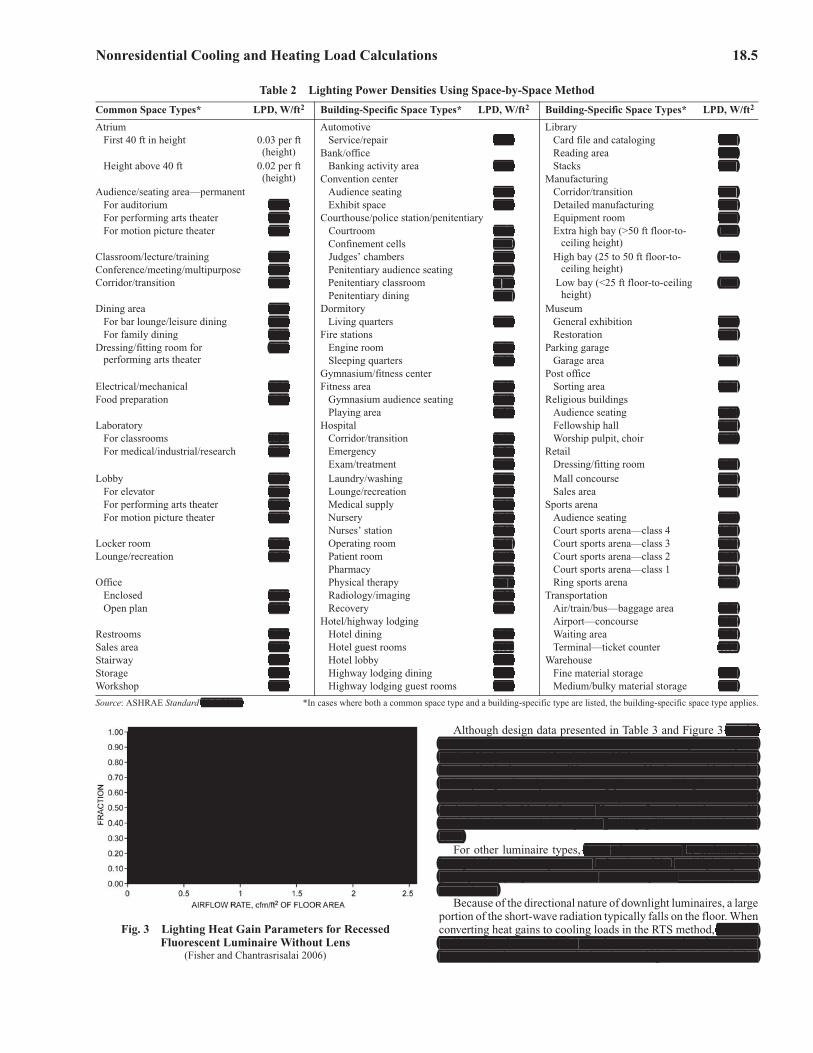
If the space airflow rate is different from the typical condition(i.e., about 1 cfm/ft2), Figure 3 can be used to estimate the lightingheat gain parameters. Design data shown in Figure 3 are only appli-cable for the recessed fluorescent luminaire without lens.
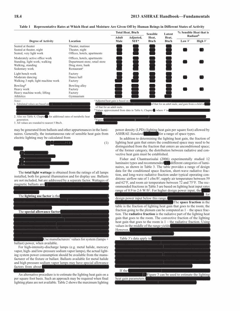
Table 1 Representative Rates at Which Heat and Moisture Are Given Off by Human Beings in Different States of Activity
Degree of Activity Location
Total Heat, Btu/h Sensible Heat,Btu/h
Latent Heat,Btu/h
% Sensible Heat that is Radiantb
AdultMale
Adjusted, M/Fa Low V High V
Seated at theater Theater, matinee 390 330 225 105Seated at theater, night Theater, night 390 350 245 105 60 27Seated, very light work Offices, hotels, apartments 450 400 245 155
Moderately active office work Offices, hotels, apartments 475 450 250 200Standing, light work; walking Department store; retail store 550 450 250 200 58 38Walking, standing Drug store, bank 550 500 250 250Sedentary work Restaurantc 490 550 275 275
Light bench work Factory 800 750 275 475Moderate dancing Dance hall 900 850 305 545 49 35Walking 3 mph; light machine work Factory 1000 1000 375 625
Bowlingd Bowling alley 1500 1450 580 870Heavy work Factory 1500 1450 580 870 54 19Heavy machine work; lifting Factory 1600 1600 635 965Athletics Gymnasium 2000 1800 710 1090
Notes:1. Tabulated values are based on 75°F room dry-bulb temperature. For
80°F room dry bulb, total heat remains the same, but sensible heatvalues should be decreased by approximately 20%, and latent heatvalues increased accordingly.
2. Also see Table 4, Chapter 9, for additional rates of metabolic heatgeneration.
3. All values are rounded to nearest 5 Btu/h.
aAdjusted heat gain is based on normal percentage of men, women, and children for the application listed,and assumes that gain from an adult female is 85% of that for an adult male, and gain from a child is 75%of that for an adult male.
b Values approximated from data in Table 6, Chapter 9, where V is air velocity with limits shown in thattable.
cAdjusted heat gain includes 60 Btu/h for food per individual (30 Btu/h sensible and 30 Btu/h latent).d Figure one person per alley actually bowling, and all others as sitting (400 Btu/h) or standing or walkingslowly (550 Btu/h).
qel = 3.41WFulFF FsaFF
whereqel = heat gain, Btu/hW = total light wattage, W
FulFF = lighting use factorFsaF = lighting special allowance factorsa
3.41 = conversion factor
60 27
58 38
49 35
54 19
390 330 225 105
450 400 245 155390 350 245 105
475 450 250 200550 450 250 200
490 550 275 275550 500 250 250
800 750 275 475
1000 1000 375 625
2000 1800 710 10901600 1600 635 965
900 850 305 545
1500 1450 580 8701500 1450 580 870
n 75°F room dry-bulb temperature. For80°F room dry bulb, total heat remains the same, but sensible heatvalues should be decreased by approximately 20%, and latent heatvalues increased accordingly.
r 9,
normal percentage of men, women, and children for the application listed,and assumes that gain from an adult female is 85% 75%
9, air velocity with limits shown in thattable.
cAdjusted heat gain includes 60 Btu/h for food per individual (30 Btu/h sensible and 30 Btu/h latent). one person per alley actually bowling, and all others as sitting (400 Btu/h) or standing or walking
slowly (550 Btu/h).
significant; the energy consumption of high-efficiency electronic ballasts might be insignificant compared tothat of the lamps.
e ratio of wattage in use, for the con-ditions under which the load estimate is being made, to totalinstalled wattage. For commercial applications such as stores, theuse factor is generally 1.0.
is the ratio of the lighting fixtures’power consumption, including lamps and ballast, to the nominalaapower consumption of the lamps. For incandescent lights, this factoris 1. For fluorescent lights, it accounts for power consumed by theballast as well as the ballast’s effect on lamp power consumption.The special allowance factor can be less than 1 for electronic bal-lasts that lower electricity consumption below the lamp’s ratedpower consumption. U
1.3 (for low-wattage lamps) down to 1.1 (forhigh-wattage lamps).
90.1-2010
d five
lowerbounds of the space and short-wave fractions should be used;
the upper bounds of the spaceand short-wave fractions should be used.
s sufficiently accurate results.values that better suit a specific situation may be deter-
mined according to the notes for Table 3.o both ducted and nonducted returns. How-
ever, application of the data, particularly the ceiling plenum frac-tion, may vary for different return configurations. For instance, forna room with a ducted return, although a portion of the lightingenergy initially dissipated to the ceiling plenum is quantitativelyequal to the plenum fraction, a large portion of this energy wouldlikely end up as the conditioned space cooling load and a small por-tion would end up as the cooling load to the return air.
space airflow rate is different from the typical conditionft2), (i.e., about 1 cfm/f
Design data shown in Figure 3 are only appli-cable for the recessed fluorescent luminaire without lens.
Nonresidential Cooling and Heating Load Calculations 18.5
Although design data presented in Table 3 and Figure 3 can beused for a vented luminaire with side-slot returns, they are likely notapplicable for a vented luminaire with lamp compartment returns,because in the latter case, all heat convected in the vented luminaireis likely to go directly to the ceiling plenum, resulting in zero con-vective fraction and a much lower space fraction. Therefore, thedesign data should only be used for a configuration where condi-tioned air is returned through the ceiling grille or luminaire sideslots.
For other luminaire types, it may be necessary to estimate theheat gain for each component as a fraction of the total lighting heatgain by using judgment to estimate heat-to-space and heat-to-returnpercentages.
Because of the directional nature of downlight luminaires, a largeportion of the short-wave radiation typically falls on the floor. Whenconverting heat gains to cooling loads in the RTS method, the solarradiant time factors (RTFs) may be more appropriate than nonso-lar RTFs. (Solar RTFs are calculated assuming most solar radiation
Table 2 Lighting Power Densities Using Space-by-Space Method
Common Space Types* LPD, W/ft2 Building-Specific Space Types* LPD, W/ft2 Building-Specific Space Types* LPD, W/ft2
Atrium Automotive LibraryFirst 40 ft in height 0.03 per ft
(height)Service/repair 0.67 Card file and cataloging 0.72
Bank/office Reading area 0.93Height above 40 ft 0.02 per ft
(height)Banking activity area 1.38 Stacks 1.71
Convention center ManufacturingAudience/seating area—permanent Audience seating 0.82 Corridor/transition 0.41
For auditorium 0.79 Exhibit space 1.45 Detailed manufacturing 1.29For performing arts theater 2.43 Courthouse/police station/penitentiary Equipment room 0.95For motion picture theater 1.14 Courtroom 1.72 Extra high bay (>50 ft floor-to-
ceiling height)1.05
Confinement cells 1.10Classroom/lecture/training 1.24 Judges’ chambers 1.17 High bay (25 to 50 ft floor-to-
ceiling height)1.23
Conference/meeting/multipurpose 1.23 Penitentiary audience seating 0.43Corridor/transition 0.66 Penitentiary classroom 1.34 Low bay (<25 ft floor-to-ceiling
height)1.19
Penitentiary dining 1.07Dining area 0.65 Dormitory Museum
For bar lounge/leisure dining 1.31 Living quarters 0.38 General exhibition 1.05For family dining 0.89 Fire stations Restoration 1.02
Dressing/fitting room for performing arts theater
0.40 Engine room 0.56 Parking garageSleeping quarters 0.25 Garage area 0.19
Gymnasium/fitness center Post officeElectrical/mechanical 0.95 Fitness area 0.72 Sorting area 0.94Food preparation 0.99 Gymnasium audience seating 0.43 Religious buildings
Playing area 1.20 Audience seating 1.53Laboratory Hospital Fellowship hall 0.64
For classrooms 1.28 Corridor/transition 0.89 Worship pulpit, choir 1.53For medical/industrial/research 1.81 Emergency 2.26 Retail
Exam/treatment 1.66 Dressing/fitting room 0.87Lobby 0.90 Laundry/washing 0.60 Mall concourse 1.10
For elevator 0.64 Lounge/recreation 1.07 Sales area 1.68For performing arts theater 2.00 Medical supply 1.27 Sports arenaFor motion picture theater 0.52 Nursery 0.88 Audience seating 0.43
Nurses’ station 0.87 Court sports arena—class 4 0.72Locker room 0.75 Operating room 1.89 Court sports arena—class 3 1.20Lounge/recreation 0.73 Patient room 0.62 Court sports arena—class 2 1.92
Pharmacy 1.14 Court sports arena—class 1 3.01Office Physical therapy 0.91 Ring sports arena 2.68
Enclosed 1.11 Radiology/imaging 1.32 TransportationOpen plan 0.98 Recovery 1.15 Air/train/bus—baggage area 0.76
Hotel/highway lodging Airport—concourse 0.36Restrooms 0.98 Hotel dining 0.82 Waiting area 0.54Sales area 1.68 Hotel guest rooms 1.11 Terminal—ticket counter 1.08Stairway 0.69 Hotel lobby 1.06 WarehouseStorage 0.63 Highway lodging dining 0.88 Fine material storage 0.95Workshop 1.59 Highway lodging guest rooms 0.75 Medium/bulky material storage 0.58
Source: ASHRAE Standard 90.1-2010. *In cases where both a common space type and a building-specific type are listed, the building-specific space type applies.
Fig. 3 Lighting Heat Gain Parameters for Recessed Fluorescent Luminaire Without Lens
(Fisher and Chantrasrisalai 2006)
can beused for a vented luminaire with side-slot returns, they are likely notapplicable for a vented luminaire with lamp compartment returns,because in the latter case, all heat convected in the vented luminaireis likely to go directly to the ceiling plenum, resulting in zero con-vective fraction and a much lower space fraction. Therefore, thedesign data should only be used for a configuration where condi-tioned air is returned through the ceiling grille or luminaire sideslots.
0.720.931.71
1.290.95
0.41
1.05
1.23
1.19
1.021.05
0.19
0.94
1.530.641.53
0.871.101.68
0.430.721.201.923.012.68
0.760.360.541.08
0.950.58
0.67
1.38
0.821.45
1.72721.101.170.431.341.07
0.38
0.560.25
0.720.431.20
0.892.261.660.601.07
0.881.27
0.871.890.621.140.911.321.15
0.82
1.061.11
0.880.75
90.1-2010.
1.590.630.691.680.98
0.981.11
0.730.75
0.522.000.640.90
1.811.28
0.792.431.14
1.241.230.66
0.651.310.890.40
0.950.99
it may be necessary to estimate theheat gain for each component as a fraction of the total lighting heatgain by using judgment to estimate heat-to-space and heat-to-returnpercentages.
the solarradiant time factors (RTFs) may be more appropriate than nonso-lar RTFs. (Solar RTFs are calculated assuming most solar radiation
18.6 2013 ASHRAE Handbook—Fundamentals
is intercepted by the floor; nonsolar RTFs assume uniform distribu-tion by area over all interior surfaces.) This effect may be significantfor rooms where lighting heat gain is high and for which solar RTFsare significantly different from nonsolar RTFs.
ELECTRIC MOTORS
Instantaneous sensible heat gain from equipment operated byelectric motors in a conditioned space is calculated as
qem = 2545(P/EM)FUM FLM (2)
whereqem = heat equivalent of equipment operation, Btu/h
P = motor power rating, hpEM = motor efficiency, decimal fraction <1.0
FUM = motor use factor, 1.0 or decimal fraction <1.0FLM = motor load factor, 1.0 or decimal fraction <1.0
2545 = conversion factor, Btu/h·hp
The motor use factor may be applied when motor use is known tobe intermittent, with significant nonuse during all hours of operation(e.g., overhead door operator). For conventional applications, itsvalue is 1.0.
The motor load factor is the fraction of the rated load deliveredunder the conditions of the cooling load estimate. Equation (2)assumes that both the motor and driven equipment are in the condi-tioned space. If the motor is outside the space or airstream,
qem = 2545PFUM FLM (3)
When the motor is inside the conditioned space or airstream butthe driven machine is outside,
qem = 2545P FUMFLM (4)
Equation (4) also applies to a fan or pump in the conditionedspace that exhausts air or pumps fluid outside that space.
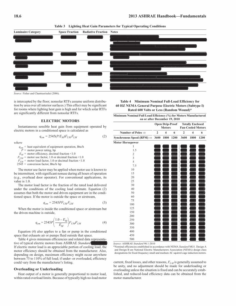
Table 4 gives minimum efficiencies and related data representa-tive of typical electric motors from ASHRAE Standard 90.1-2010.If electric motor load is an appreciable portion of cooling load, themotor efficiency should be obtained from the manufacturer. Also,depending on design, maximum efficiency might occur anywherebetween 75 to 110% of full load; if under- or overloaded, efficiencycould vary from the manufacturer’s listing.
Overloading or UnderloadingHeat output of a motor is generally proportional to motor load,
within rated overload limits. Because of typically high no-load motor
current, fixed losses, and other reasons, FLM is generally assumed tobe unity, and no adjustment should be made for underloading oroverloading unless the situation is fixed and can be accurately estab-lished, and reduced-load efficiency data can be obtained from themotor manufacturer.
Table 3 Lighting Heat Gain Parameters for Typical Operating Conditions
Luminaire Category Space Fraction Radiative Fraction Notes
Recessed fluorescent luminaire without lens
0.64 to 0.74 0.48 to 0.68 • Use middle values in most situations• May use higher space fraction, and lower radiative fraction for luminaire
with side-slot returns• May use lower values of both fractions for direct/indirect luminaire• May use higher values of both fractions for ducted returns
Recessed fluorescent luminaire with lens
0.40 to 0.50 0.61 to 0.73 • May adjust values in the same way as for recessed fluorescent luminairewithout lens
Downlight compact fluorescent luminaire
0.12 to 0.24 0.95 to 1.0 • Use middle or high values if detailed features are unknown• Use low value for space fraction and high value for radiative fraction if there
are large holes in luminaire’s reflector
Downlight incandescent luminaire
0.70 to 0.80 0.95 to 1.0 • Use middle values if lamp type is unknown• Use low value for space fraction if standard lamp (i.e. A-lamp) is used• Use high value for space fraction if reflector lamp (i.e. BR-lamp) is used
Non-in-ceiling fluorescent luminaire
1.0 0.5 to 0.57 • Use lower value for radiative fraction for surface-mounted luminaire• Use higher value for radiative fraction for pendant luminaire
Source: Fisher and Chantrasrisalai (2006).
1.0 EM–
EM---------------------� �� �� �
Table 4 Minimum Nominal Full-Load Efficiency for60 HZ NEMA General Purpose Electric Motors (Subtype I)
Rated 600 Volts or Less (Random Wound)*
Minimum Nominal Full Load Efficiency (%) for Motors Manufactured on or after December 19, 2010
Open Drip-Proof Motors
Totally Enclosed Fan-Cooled Motors
Number of Poles � 2 4 6 2 4 6
Synchronous Speed (RPM) � 3600 1800 1200 3600 1800 1200
Motor Horsepower1 77.0 85.5 82.5 77.0 85.5 82.51.5 84.0 86.5 86.5 84.0 86.5 87.52 85.5 86.5 87.5 85.5 86.5 88.53 85.5 89.5 88.5 86.5 89.5 89.55 86.5 89.5 89.5 88.5 89.5 89.57.5 88.5 91.0 90.2 89.5 91.7 91.0
10 89.5 91.7 91.7 90.2 91.7 91.015 90.2 93.0 91.7 91.0 92.4 91.720 91.0 93.0 92.4 91.0 93.0 91.725 91.7 93.6 93.0 91.7 93.6 93.030 91.7 94.1 93.6 91.7 93.6 93.040 92.4 94.1 94.1 92.4 94.1 94.150 93.0 94.5 94.1 93.0 94.5 94.160 93.6 95.0 94.5 93.6 95.0 94.575 93.6 95.0 94.5 93.6 95.4 94.5
100 93.6 95.4 95.0 94.1 95.4 95.0125 94.1 95.4 95.0 95.0 95.4 95.0150 94.1 95.8 95.4 95.0 95.8 95.8200 95.0 95.8 95.4 95.4 96.2 95.8250 95.0 95.8 95.4 95.8 96.2 95.8300 95.4 95.8 95.4 95.8 96.2 95.8350 95.4 95.8 95.4 95.8 96.2 95.8400 95.8 95.8 95.8 95.8 96.2 95.8450 95.8 96.2 96.2 95.8 96.2 95.8500 95.8 96.2 96.2 95.8 96.2 95.8
Source: ASHRAE Standard 90.1-2010*Nominal efficiencies established in accordance with NEMA Standard MG1. Design Aand Design B are National Electric Manufacturers Association (NEMA) design classdesignations for fixed-frequency small and medium AC squirrel-cage induction motors.
• Use middle values in most situationsRecessed fluorescent luminaire 0.64 to 0.74 0.48 to 0.68• May use higher space fraction, and lower radiative fraction for luminairewithout lens y g p
with side-slot returns• May use lower values of both fractions for direct/indirect luminairey• May use higher values of both fractions for ducted returns
Recessed fluorescent luminaire 0.40 to 0.50 0.61 to 0.73 • May adjust values in the same way as for recessed fluorescent luminairey jwithout lenswith lens
Downlight compact fluorescent 0.12 to 0.24 0.95 to 1.0 • Use middle or high values if detailed features are unknowng• Use low value for space fraction and high value for radiative fraction if therehluminaire p g
are large holes in luminaire’s reflector
Downlight incandescent 0.70 to 0.80 0.95 to 1.0 • Use middle values if lamp type is unknownp yp• Use low value for space fraction if standard lamp (i.e. A-lamp) is usedluminaire p p ( p)• Use high value for space fraction if reflector lamp (i.e. BR-lamp) is used
Non-in-ceiling fluorescent 1.0 0.5 to 0.57 • Use lower value for radiative fraction for surface-mounted luminaire• Use higher value for radiative fraction for pendant luminaireluminaire
90.1-2010.
77.0 85.5 82.5 77.0 85.5 82.584.0 86.5 86.5 84.0 86.5 87.585.5 86.5 87.5 85.5 86.5 88.585.5 89.5 88.5 86.5 89.5 89.586.5 89.5 89.5 88.5 89.5 89.588.5 91.0 90.2 89.5 91.7 91.089.5 91.7 91.7 90.2 91.7 91.090.2 93.0 91.7 91.0 92.4 91.791.0 93.0 92.4 91.0 93.0 91.791.7 93.6 93.0 91.7 93.6 93.091.7 94.1 93.6 91.7 93.6 93.092.4 94.1 94.1 92.4 94.1 94.193.0 94.5 94.1 93.0 94.5 94.193.6 95.0 94.5 93.6 95.0 94.593.6 95.0 94.5 93.6 95.4 94.593.6 95.4 95.0 94.1 95.4 95.094.1 95.4 95.0 95.0 95.4 95.094.1 95.8 95.4 95.0 95.8 95.895.0 95.8 95.4 95.4 96.2 95.895.0 95.8 95.4 95.8 96.2 95.895.4 95.8 95.4 95.8 96.2 95.895.4 95.8 95.4 95.8 96.2 95.895.8 95.8 95.8 95.8 96.2 95.895.8 96.2 96.2 95.8 96.2 95.895.8 96.2 96.2 95.8 96.2 95.8
Nonresidential Cooling and Heating Load Calculations 18.7
Radiation and ConvectionUnless the manufacturer’s technical literature indicates other-
wise, motor heat gain normally should be equally divided betweenradiant and convective components for the subsequent cooling loadcalculations.
APPLIANCES
A cooling load estimate should take into account heat gain fromall appliances (electrical, gas, or steam). Because of the variety ofappliances, applications, schedules, use, and installations, estimatescan be very subjective. Often, the only information available aboutheat gain from equipment is that on its nameplate, which can over-estimate actual heat gain for many types of appliances, as discussedin the section on Office Equipment.
Cooking AppliancesThese appliances include common heat-producing cooking
equipment found in conditioned commercial kitchens. Marn (1962)concluded that appliance surfaces contributed most of the heat tocommercial kitchens and that when appliances were installed underan effective hood, the cooling load was independent of the fuel orenergy used for similar equipment performing the same operations.
Gordon et al. (1994) and Smith et al. (1995) found that gas appli-ances may exhibit slightly higher heat gains than their electric coun-terparts under wall-canopy hoods operated at typical ventilationrates. This is because heat contained in combustion products ex-hausted from a gas appliance may increase the temperatures of theappliance and surrounding surfaces, as well as the hood above the ap-pliance, more so than the heat produced by its electric counterpart.These higher-temperature surfaces radiate heat to the kitchen, addingmoderately to the radiant gain directly associated with the appliancecooking surface.
Marn (1962) confirmed that, where appliances are installedunder an effective hood, only radiant gain adds to the cooling load;convective and latent heat from cooking and combustion productsare exhausted and do not enter the kitchen. Gordon et al. (1994) andSmith et al. (1995) substantiated these findings. Chapter 33 of the2011 ASHRAE Handbook—HVAC Applications has more informa-tion on kitchen ventilation.
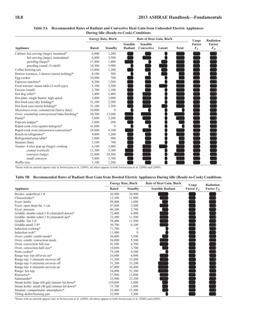
Sensible Heat Gain for Hooded Cooking Appliances. Toestablish a heat gain value, nameplate energy input ratings may beused with appropriate usage and radiation factors. Where specificrating data are not available (nameplate missing, equipment not yetpurchased, etc.), representative heat gains listed in Tables 5A to E(Swierczyna et al. 2008, 2009) for a wide variety of commonlyencountered equipment items. In estimating appliance load, proba-bilities of simultaneous use and operation for different applianceslocated in the same space must be considered.
Radiant heat gain from hooded cooking equipment can rangefrom 15 to 45% of the actual appliance energy consumption (Gor-don et al. 1994; Smith et al. 1995; Swierczyna et al. 2008; Talbertet al. 1973). This ratio of heat gain to appliance energy consumptionmay be expressed as a radiation factor, and it is a function of bothappliance type and fuel source. The radiation factor FR is applied tothe average rate of appliance energy consumption, determined byapplying usage factor FU to the nameplate or rated energy input.Marn (1962) found that radiant heat temperature rise can be sub-stantially reduced by shielding the fronts of cooking appliances.Although this approach may not always be practical in a commer-cial kitchen, radiant gains can also be reduced by adding side panelsor partial enclosures that are integrated with the exhaust hood.
Heat Gain from Meals. For each meal served, approximately50 Btu/h of heat, of which 75% is sensible and 25% is latent, istransferred to the dining space.
Heat Gain for Generic Appliances. The average rate of appli-ance energy consumption can be estimated from the nameplate orrated energy input qinput by applying a duty cycle or usage factor FU.Thus, sensible heat gain qs for generic electric, steam, and gas appli-ances installed under a hood can be estimated using one of the fol-lowing equations:
qs = qinput FU FR (5)
or
qs = qinput FL (6)
where FL is the ratio of sensible heat gain to the manufacturer’srated energy input. However, recent ASHRAE research (Swierc-zyna et al. 2008, 2009) showed the design value for heat gain froma hooded appliance at idle (ready-to-cook) conditions based on itsenergy consumption rate is, at best, a rough estimate. When appli-ance heat gain measurements during idle conditions were regressedagainst energy consumption rates for gas and electric appliances,the appliances’ emissivity, insulation, and surface cooling (e.g.,through ventilation rates) scattered the data points widely, withlarge deviations from the average values. Because large errors couldoccur in the heat load calculation for specific appliance lines byusing a general radiation factor, heat gain values in Table 5 shouldbe applied in the HVAC design.
Table 5 lists usage factors, radiation factors, and load factorsbased on appliance energy consumption rate for typical electrical,steam, and gas appliances under standby or idle conditions, hoodedand unhooded.
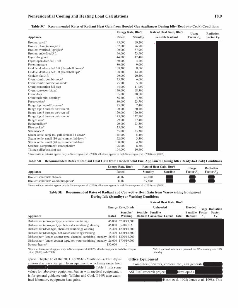
Recirculating Systems. Cooking appliances ventilated by recir-culating systems or “ductless” hoods should be treated as unhoodedappliances when estimating heat gain. In other words, all energyconsumed by the appliance and all moisture produced by cooking isintroduced to the kitchen as a sensible or latent cooling load.
Recommended Heat Gain Values. Table 5 lists recommendedrates of heat gain from typical commercial cooking appliances. Datain the “hooded” columns assume installation under a properly de-signed exhaust hood connected to a mechanical fan exhaust systemoperating at an exhaust rate for complete capture and containmentof the thermal and effluent plume. Improperly operating hood sys-tems load the space with a significant convective component of theheat gain.
Hospital and Laboratory EquipmentHospital and laboratory equipment items are major sources of
sensible and latent heat gains in conditioned spaces. Care is neededin evaluating the probability and duration of simultaneous usagewhen many components are concentrated in one area, such as a lab-oratory, an operating room, etc. Commonly, heat gain from equip-ment in a laboratory ranges from 15 to 70 Btu/h·ft2 or, in laboratorieswith outdoor exposure, as much as four times the heat gain from allother sources combined.
Medical Equipment. It is more difficult to provide generalizedheat gain recommendations for medical equipment than for generaloffice equipment because medical equipment is much more variedin type and in application. Some heat gain testing has been done, butthe equipment included represents only a small sample of the type ofequipment that may be encountered.
Data presented for medical equipment in Table 6 are relevant forportable and bench-top equipment. Medical equipment is very spe-cific and can vary greatly from application to application. The dataare presented to provide guidance in only the most general sense.For large equipment, such as MRI, heat gain must be obtained fromthe manufacturer.
Laboratory Equipment. Equipment in laboratories is similar tomedical equipment in that it varies significantly from space to
appliance surfaces contributed most of the heat tocommercial kitchens and that when appliances weren installed underan effective hood, the cooling load was independent of the fuel orenergy used for similar equipment performing the same operations.
t gas appli-ances may exhibit slightly higher heat gains than their electric coun-terparts under wall-canopy hoods operated at typical ventilationrates. This is because heat contained in combustion products ex-hausted from a gas appliance may increase the temperatures of theappliance and surrounding surfaces, as well as the hood above the ap-pliance, more so than the heat produced by its electric counterpart.These higher-temperature surfaces radiate heat to the kitchen, addingmoderately to the radiant gain directly associated with the appliancecooking surface.
where appliances are installedunder an effective hood, only radiant gain adds to the cooling load;convective and latent heat from cooking and combustion productsare exhausted and do not enter the kitchen. G
33
kitchen ventilation.
proba-bilities of simultaneous use and operation for different applianceslocated in the same space must be considered.
Radiant heat gain from hooded cooking equipment can rangefrom 15 to 45% of the actual appliance energy consumption (
radiation factor, and it is a function of bothappliance type and fuel source. The radiation factor r FRFF is applied toRthe average rate of appliance energy consumption, determined byapplying usage factor FUFF U to the nameplate or rated energy input.UMarn (1962) found that radiant heat temperature rise can be sub-tstantially reduced by shielding the fronts of cooking appliances.Although this approach may not always be practical in a commer-cial kitchen, radiant gains can also be reduced by adding side panelsor partial enclosures that are integrated with the exhaust hood.
For each meal served, approximately50 Btu/h of heat, of which 75% is sensible and 25% is latent, istransferred to the dining space.
nameplate orrated energy inputt qinput tt by applying a duty cycle or usage factor t r FUFF .pThus, sensible heat gainn qs for generic electric, steam, and gas appli-ances installed under a hood can be estimated u
qs = qinput Ft UFF FRFF
qs = qinput Ft LF
FLF is the ratio of sensible heat gain to the manufacturer’sLrated energy input.
design value for heat gain froma hooded appliance at idle (ready-to-cook) conditions based on itsenergy consumption rate is, at best, a rough estimate. When appli-ance heat gain measurements during idle conditions were regressedagainst energy consumption rates for gas and electric appliances,the appliances’ emissivity, insulation, and surface cooling (e.g.,through ventilation rates) scattered the data points widely, withlarge deviations from the average values. B
treated as unhoodedappliances when estimating heat gain. I all energyconsumed by the appliance and all moisture produced by cooking isintroduced to the kitchen as a sensible or latent cooling load.
major sources ofsensible and latent heat gains in conditioned spaces.
evaluating the probability and duration of simultaneous usagewhen many components are concentrated in one area, such as a lab-oratory, an operating room, etc. Commonly, heat gain from equip-
ft2 ment in a laboratory ranges from 15 to 70 Btu/h·f or, in laboratorieswith outdoor exposure, as much as four times the heat gain from allother sources combined.
portable and bench-top equipment. Medical equipment is very spe-cific and can vary greatly from application to application.
it varies significantly from space to
18.8 2013 ASHRAE Handbook—Fundamentals
Table 5A Recommended Rates of Radiant and Convective Heat Gain from Unhooded Electric Appliances During Idle (Ready-to-Cook) Conditions
Appliance
Energy Rate, Btu/h Rate of Heat Gain, Btu/h Usage Factor
FU
Radiation Factor
FRRated StandbySensible Radiant
Sensible Convective Latent Total
Cabinet: hot serving (large), insulated* 6,800 1,200 400 800 0 1,200 0.18 0.33hot serving (large), uninsulated 6,800 3,500 700 2,800 0 3,500 0.51 0.20proofing (large)* 17,400 1,400 1,200 0 200 1,400 0.08 0.86proofing (small 15-shelf) 14,300 3,900 0 900 3,000 3,900 0.27 0.00
Coffee brewing urn 13,000 1,200 200 300 700 1,200 0.09 0.17Drawer warmers, 2-drawer (moist holding)* 4,100 500 0 0 200 200 0.12 0.00Egg cooker 10,900 700 300 400 0 700 0.06 0.43Espresso machine* 8,200 1,200 400 800 0 1,200 0.15 0.33Food warmer: steam table (2-well-type) 5,100 3,500 300 600 2,600 3,500 0.69 0.09Freezer (small) 2,700 1,100 500 600 0 1,100 0.41 0.45Hot dog roller* 3,400 2,400 900 1,500 0 2,400 0.71 0.38Hot plate: single burner, high speed 3,800 3,000 900 2,100 0 3,000 0.79 0.30Hot-food case (dry holding)* 31,100 2,500 900 1,600 0 2,500 0.08 0.36Hot-food case (moist holding)* 31,100 3,300 900 1,800 600 3,300 0.11 0.27Microwave oven: commercial (heavy duty) 10,900 0 0 0 0 0 0.00 0.00Oven: countertop conveyorized bake/finishing* 20,500 12,600 2,200 10,400 0 12,600 0.61 0.17Panini* 5,800 3,200 1,200 2,000 0 3,200 0.55 0.38Popcorn popper* 2,000 200 100 100 0 200 0.10 0.50Rapid-cook oven (quartz-halogen)* 41,000 0 0 0 0 0 0.00 0.00Rapid-cook oven (microwave/convection)* 24,900 4,100 1,000 3,100 0 1,000 0.16 0.24Reach-in refrigerator* 4,800 1,200 300 900 0 1,200 0.25 0.25Refrigerated prep table* 2,000 900 600 300 0 900 0.45 0.67Steamer (bun) 5,100 700 600 100 0 700 0.14 0.86Toaster: 4-slice pop up (large): cooking 6,100 3,000 200 1,400 1,000 2,600 0.49 0.07
contact (vertical) 11,300 5,300 2,700 2,600 0 5,300 0.47 0.51conveyor (large) 32,800 10,300 3,000 7,300 0 10,300 0.31 0.29small conveyor 5,800 3,700 400 3,300 0 3,700 0.64 0.11
Waffle iron 3,100 1,200 800 400 0 1,200 0.39 0.67
*Items with an asterisk appear only in Swierczyna et al. (2009); all others appear in both Swierczyna et al. (2008) and (2009).
Table 5B Recommended Rates of Radiant Heat Gain from Hooded Electric Appliances During Idle (Ready-to-Cook) Conditions
Appliance
Energy Rate, Btu/h Rate of Heat Gain, Btu/h UsageFactor FU
Radiation Factor FRRated Standby Sensible Radiant
Broiler: underfired 3 ft 36,900 30,900 10,800 0.84 0.35Cheesemelter* 12,300 11,900 4,600 0.97 0.39Fryer: kettle 99,000 1,800 500 0.02 0.28Fryer: open deep-fat, 1-vat 47,800 2,800 1,000 0.06 0.36Fryer: pressure 46,100 2,700 500 0.06 0.19Griddle: double sided 3 ft (clamshell down)* 72,400 6,900 1,400 0.10 0.20Griddle: double sided 3 ft (clamshell up)* 72,400 11,500 3,600 0.16 0.31Griddle: flat 3 ft 58,400 11,500 4,500 0.20 0.39Griddle-small 3 ft* 30,700 6,100 2,700 0.20 0.44Induction cooktop* 71,700 0 0 0.00 0.00Induction wok* 11,900 0 0 0.00 0.00Oven: combi: combi-mode* 56,000 5,500 800 0.10 0.15Oven: combi: convection mode 56,000 5,500 1,400 0.10 0.25Oven: convection full-size 41,300 6,700 1,500 0.16 0.22Oven: convection half-size* 18,800 3,700 500 0.20 0.14Pasta cooker* 75,100 8,500 0 0.11 0.00Range top: top off/oven on* 16,600 4,000 1,000 0.24 0.25Range top: 3 elements on/oven off 51,200 15,400 6,300 0.30 0.41Range top: 6 elements on/oven off 51,200 33,200 13,900 0.65 0.42Range top: 6 elements on/oven on 67,800 36,400 14,500 0.54 0.40Range: hot-top 54,000 51,300 11,800 0.95 0.23Rotisserie* 37,900 13,800 4,500 0.36 0.33Salamander* 23,900 23,300 7,000 0.97 0.30Steam kettle: large (60 gal) simmer lid down* 110,600 2,600 100 0.02 0.04Steam kettle: small (40 gal) simmer lid down* 73,700 1,800 300 0.02 0.17Steamer: compartment: atmospheric* 33,400 15,300 200 0.46 0.01Tilting skillet/braising pan 32,900 5,300 0 0.16 0.00
*Items with an asterisk appear only in Swierczyna et al. (2009); all others appear in both Swierczyna et al. (2008) and (2009).
400 800 0 1,200 0.18 0.33
1,200 0 200 1,400 0.08 0.86700 2,800 0 3,500 0.51 0.20
0 900 3,000 3,900 0.27 0.00200 300 700 1,200 0.09 0.17
0 0 200 200 0.12 0.00300 400 0 700 0.06 0.43400 800 0 1,200 0.15 0.33300 600 2,600 3,500 0.69 0.09500 600 0 1,100 0.41 0.45900 1,500 0 2,400 0.71 0.38900 2,100 0 3,000 0.79 0.30900 1,600 0 2,500 0.08 0.36900 1,800 600 3,300 0.11 0.27
0 0 0 0 0.00 0.002,200 10,400 0 12,600 0.61 0.171,200 2,000 0 3,200 0.55 0.38
100 100 0 200 0.10 0.500 0 0 0 0.00 0.00
1,000 3,100 0 1,000 0.16 0.24300 900 0 1,200 0.25 0.25600 300 0 900 0.45 0.67600 100 0 700 0.14 0.86200 1,400 1,000 2,600 0.49 0.07
2,700 2,600 0 5,300 0.47 0.513,000 7,300 0 10,300 0.31 0.29
400 3,300 0 3,700 0.64 0.11800 400 0 1,200 0.39 0.67
10,800 0.84 0.354,600 0.97 0.39
1,000 0.06 0.36500 0.02 0.28
1,400 0.10 0.203,600 0.16 0.31
500 0.06 0.19
4,500 0.20 0.392,700 0.20 0.44
0 0.00 0.000 0.00 0.00
800 0.10 0.151,400 0.10 0.251,500 0.16 0.22
500 0.20 0.140 0.11 0.00
1,000 0.24 0.256,300 0.30 0.41
13,900 0.65 0.4214,500 0.54 0.4011,800 0.95 0.234,500 0.36 0.337,000 0.97 0.30
100 0.02 0.04
200 0.46 0.01300 0.02 0.17
0 0.16 0.00
Nonresidential Cooling and Heating Load Calculations 18.9
space. Chapter 16 of the 2011 ASHRAE Handbook—HVAC Appli-cations discusses heat gain from equipment, which may range from5 to 25 W/ft2 in highly automated laboratories. Table 7 lists somevalues for laboratory equipment, but, as with medical equipment, itis for general guidance only. Wilkins and Cook (1999) also exam-ined laboratory equipment heat gains.
Office EquipmentComputers, printers, copiers, etc., can generate very signifi-
cant heat gains, sometimes greater than all other gains combined.ASHRAE research project RP-822 developed a method to measurethe actual heat gain from equipment in buildings and the radiant/convective percentages (Hosni et al. 1998; Jones et al. 1998). This
Table 5C Recommended Rates of Radiant Heat Gain from Hooded Gas Appliances During Idle (Ready-to-Cook) Conditions
Appliance
Energy Rate, Btu/h Rate of Heat Gain, Btu/h UsageFactor FU
Radiation Factor FRRated Standby Sensible Radiant
Broiler: batch* 95,000 69,200 8,100 0.73 0.12Broiler: chain (conveyor) 132,000 96,700 13,200 0.73 0.14Broiler: overfired (upright)* 100,000 87,900 2,500 0.88 0.03Broiler: underfired 3 ft 96,000 73,900 9,000 0.77 0.12Fryer: doughnut 44,000 12,400 2,900 0.28 0.23Fryer: open deep-fat, 1 vat 80,000 4,700 1,100 0.06 0.23Fryer: pressure 80,000 9,000 800 0.11 0.09Griddle: double sided 3 ft (clamshell down)* 108,200 8,000 1,800 0.07 0.23Griddle: double sided 3 ft (clamshell up)* 108,200 14,700 4,900 0.14 0.33Griddle: flat 3 ft 90,000 20,400 3,700 0.23 0.18Oven: combi: combi-mode* 75,700 6,000 400 0.08 0.07Oven: combi: convection mode 75,700 5,800 1,000 0.08 0.17Oven: convection full-size 44,000 11,900 1,000 0.27 0.08Oven: conveyor (pizza) 170,000 68,300 7,800 0.40 0.11Oven: deck 105,000 20,500 3,500 0.20 0.17Oven: rack mini-rotating* 56,300 4,500 1,100 0.08 0.24Pasta cooker* 80,000 23,700 0 0.30 0.00Range top: top off/oven on* 25,000 7,400 2,000 0.30 0.27Range top: 3 burners on/oven off 120,000 60,100 7,100 0.50 0.12Range top: 6 burners on/oven off 120,000 120,800 11,500 1.01 0.10Range top: 6 burners on/oven on 145,000 122,900 13,600 0.85 0.11Range: wok* 99,000 87,400 5,200 0.88 0.06Rethermalizer* 90,000 23,300 11,500 0.26 0.49Rice cooker* 35,000 500 300 0.01 0.60Salamander* 35,000 33,300 5,300 0.95 0.16Steam kettle: large (60 gal) simmer lid down* 145,000 5,400 0 0.04 0.00Steam kettle: small (10 gal) simmer lid down* 52,000 3,300 300 0.06 0.09Steam kettle: small (40 gal) simmer lid down 100,000 4,300 0 0.04 0.00Steamer: compartment: atmospheric* 26,000 8,300 0 0.32 0.00Tilting skillet/braising pan 104,000 10,400 400 0.10 0.04
*Items with an asterisk appear only in Swierczyna et al. (2009); all others appear in both Swierczyna et al. (2008) and (2009).
Table 5D Recommended Rates of Radiant Heat Gain from Hooded Solid Fuel Appliances During Idle (Ready-to-Cook) Conditions
Appliance
Energy Rate, Btu/h Rate of Heat Gain, Btu/h Usage Factor FU
Radiation Factor FRRated Standby Sensible
Broiler: solid fuel: charcoal 40 lb 42,000 6200 N/A 0.15Broiler: solid fuel: wood (mesquite)* 40 lb 49,600 7000 N/A 0.14
*Items with an asterisk appear only in Swierczyna et al. (2009); all others appear in both Swierczyna et al. (2008) and (2009).
Table 5E Recommended Rates of Radiant and Convective Heat Gain from Warewashing Equipment During Idle (Standby) or Washing Conditions
Appliance
Energy Rate, Btu/h
Rate of Heat Gain, Btu/h
Usage Factor
FU
Radiation Factor
FR
Unhooded Hooded
RatedStandby/ Washing
Sensible Radiant
Sensible Convective Latent Total
Sensible Radiant
Dishwasher (conveyor type, chemical sanitizing) 46,800 5700/43,600 0 4450 13490 17940 0 0.36 0Dishwasher (conveyor type, hot-water sanitizing) standby 46,800 5700/N/A 0 4750 16970 21720 0 N/A 0Dishwasher (door-type, chemical sanitizing) washing 18,400 1200/13,300 0 1980 2790 4770 0 0.26 0Dishwasher (door-type, hot-water sanitizing) washing 18,400 1200/13,300 0 1980 2790 4770 0 0.26 0Dishwasher* (under-counter type, chemical sanitizing) standby 26,600 1200/18,700 0 2280 4170 6450 0 0.35 0.00Dishwasher* (under-counter type, hot-water sanitizing) standby 26,600 1700/19,700 800 1040 3010 4850 800 0.27 0.34Booster heater* 130,000 0 500 0 0 0 500 0 N/A
*Items with an asterisk appear only in Swierczyna et al. (2009); all others appear in both Swierczynaet al. (2008) and (2009).
Note: Heat load values are prorated for 30% washing and 70%standby.
6200 N/A 0.157000 N/A 0.14
ft2 5 to 25 W/f in highly automated laboratories.very signifi-
cant heat gains, sometimes greater than all other gains combined.t RP-822 a method to measure
the actual heat gain from equipment in buildings and the radiant/convective percentages (

18.10 2013 ASHRAE Handbook—Fundamentals
methodology was then incorporated into ASHRAE research projectRP-1055 and applied to a wide range of equipment (Hosni et al.1999) as a follow-up to independent research by Wilkins andMcGaffin (1994) and Wilkins et al. (1991). Komor (1997) foundsimilar results. Analysis of measured data showed that results foroffice equipment could be generalized, but results from laboratoryand hospital equipment proved too diverse. The following generalguidelines for office equipment are a result of these studies.
Nameplate Versus Measured Energy Use. Nameplate datararely reflect the actual power consumption of office equipment.
Actual power consumption is assumed to equal total (radiant plusconvective) heat gain, but its ratio to the nameplate value varieswidely. ASHRAE research project RP-1055 (Hosni et al. 1999)found that, for general office equipment with nameplate power con-sumption of less than 1000 W, the actual ratio of total heat gain tonameplate ranged from 25% to 50%, but when all tested equipmentis considered, the range is broader. Generally, if the nameplate valueis the only information known and no actual heat gain data are avail-able for similar equipment, it is conservative to use 50% of name-plate as heat gain and more nearly correct if 25% of nameplate isused. Much better results can be obtained, however, by consideringheat gain to be predictable based on the type of equipment. How-ever, if the device has a mainly resistive internal electric load (e.g.,a space heater), the nameplate rating may be a good estimate of itspeak energy dissipation.
Computers. Based on tests by Hosni et al. (1999) and Wilkinsand McGaffin (1994), nameplate values on computers should beignored when performing cooling load calculations. Table 8 pres-ents typical heat gain values for computers with varying degrees ofsafety factor.
Monitors. Based on monitors tested by Hosni et al. (1999), heatgain for cathode ray tube (CRT) monitors correlates approximatelywith screen size as
qmon = 5S – 20 (7)
whereqmon = sensible heat gain from monitor, W
S = nominal screen size, in.
Table 8 shows typical values.Flat-panel monitors have replaced CRT monitors in many work-
places. Power consumption, and thus heat gain, for flat-panel dis-plays are significantly lower than for CRTs. Consult manufacturers’literature for average power consumption data for use in heat gaincalculations.
Laser Printers. Hosni et al. (1999) found that power consump-tion, and therefore the heat gain, of laser printers depended largelyon the level of throughput for which the printer was designed.Smaller printers tend to be used more intermittently, and largerprinters may run continuously for longer periods.
Table 9 presents data on laser printers. These data can be appliedby taking the value for continuous operation and then applying anappropriate diversity factor. This would likely be most appropriatefor larger open office areas. Another approach, which may beappropriate for a single room or small area, is to take the value thatmost closely matches the expected operation of the printer with nodiversity.
Copiers. Hosni et al. (1999) also tested five photocopymachines, including desktop and office (freestanding high-volumecopiers) models. Larger machines used in production environmentswere not addressed. Table 9 summarizes the results. Desktop copi-ers rarely operate continuously, but office copiers frequently operatecontinuously for periods of an hour or more. Large, high-volumephotocopiers often include provisions for exhausting air outdoors; ifso equipped, the direct-to-space or system makeup air heat gainneeds to be included in the load calculation. Also, when the air isdry, humidifiers are often operated near copiers to limit static elec-tricity; if this occurs during cooling mode, their load on HVAC sys-tems should be considered.
Miscellaneous Office Equipment. Table 10 presents data onmiscellaneous office equipment such as vending machines andmailing equipment.
Diversity. The ratio of measured peak electrical load at equip-ment panels to the sum of the maximum electrical load of eachindividual item of equipment is the usage diversity. A small, one- ortwo-person office containing equipment listed in Tables 8 to 10
Table 6 Recommended Heat Gain from Typical Medical Equipment
Equipment Nameplate, W Peak, W Average, W
Anesthesia system 250 177 166Blanket warmer 500 504 221Blood pressure meter 180 33 29Blood warmer 360 204 114ECG/RESP 1440 54 50Electrosurgery 1000 147 109Endoscope 1688 605 596Harmonical scalpel 230 60 59Hysteroscopic pump 180 35 34Laser sonics 1200 256 229Optical microscope 330 65 63Pulse oximeter 72 21 20Stress treadmill N/A 198 173Ultrasound system 1800 1063 1050Vacuum suction 621 337 302X-ray system 968 82
1725 534 4802070 18
Source: Hosni et al. (1999).
Table 7 Recommended Heat Gain from Typical Laboratory Equipment
Equipment Nameplate, W Peak, W Average, W
Analytical balance 7 7 7Centrifuge 138 89 87
288 136 1325500 1176 730
Electrochemical analyzer 50 45 44100 85 84
Flame photometer 180 107 105Fluorescent microscope 150 144 143
200 205 178Function generator 58 29 29Incubator 515 461 451
600 479 2643125 1335 1222
Orbital shaker 100 16 16Oscilloscope 72 38 38
345 99 97Rotary evaporator 75 74 73
94 29 28Spectronics 36 31 31Spectrophotometer 575 106 104
200 122 121N/A 127 125
Spectro fluorometer 340 405 395Thermocycler 1840 965 641
N/A 233 198Tissue culture 475 132 46
2346 1178 1146
Source: Hosni et al. (1999).
methodology wRP-1055 applied to a wide range of equipment (Hosni et al.1999) as a follow-up to independent research by Wilkins andMcGaffin (1994) and Wilkins et al. (1991). Komor (1997) foundsimilar results. Analysis of measured data showed that results foroffice equipment could be generalized, but results from laboratoryand hospital equipment proved too diverse.
Nameplate datararely reflect the actual power consumption of office equipment.
Actual power consumption is assumed to equal total (radiant plusconvective) heat gain, but its ratio to the nameplate value varieswidely. ASHRAE research project RP-1055 (Hosni et al. 1999)found that, for general office equipment with nameplate power con-sumption of less than 1000 W, the actual ratio of total heat gain tonameplate ranged from 25% to 50%, but when all tested equipmentis considered, the range is broader. Generally, if the nameplate valueis the only information known and no actual heat gain data are avail-able for similar equipment, it is conservative to use 50% of name-plate as heat gain and more nearly correct if 25% of nameplate isused. Much better results can be obtained, however, by consideringheat gain to be predictable based on the type of equipment. How-ever, if the device has a mainly resistive internal electric load (e.g.,a space heater), the nameplate rating may be a good estimate of itspeak energy dissipation.
nameplate values on computers should beignored when performing cooling load calculations. Table 8 pres-ents typical heat gain values for computers with varying degrees ofsafety factor.
heatgain for cathode ray tube (CRT) monitors correlates approximatelywith screen size as
qmon = 5S – 20S (7)
whereqmon = sensible heat gain from monitor, W
S = nominal screen size, in.
e significantly lower than for CRTs. Consult manufacturers’nliterature for average power consumption data for use in heat gaincalculations.
that power consump-tion, and therefore the heat gain, of laser printers depended largelyon the level of throughput for which the printer was designed.Smaller printers tend to be used more intermittently, and largerprinters may run continuously for longer periods.
e appliedby taking the value for continuous operation and then applying anappropriate diversity factor. This would likely be most appropriatefor larger open office areas. Another approach, which may beappropriate for a single room or small area, is to take the value thatmost closely matches the expected operation of the printer with nodiversity.
desktop and office (freestanding high-volumecopiers) models. Larger machines used in production environmentswere not addressed. Table 9 summarizes the results. Desktop copi-ers rarely operate continuously, but office copiers frequently operatecontinuously for periods of an hour or more. Large, high-volumephotocopiers often include provisions for exhausting air outdoors; ifso equipped, the direct-to-space or system makeup air heat gainneeds to be included in the load calculation. Also, when the air isdry, humidifiers are often operated near copiers to limit static elec-tricity; if this occurs during cooling mode, their load on HVAC sys-tems should be considered.
vending machines andmailing equipment.
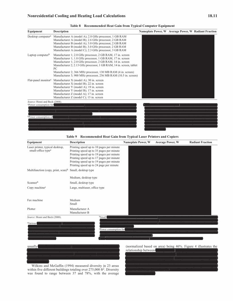
Nonresidential Cooling and Heating Load Calculations 18.11
usually contributes heat gain to the space at the sum of the appro-priate listed values. Progressively larger areas with many equipmentitems always experience some degree of usage diversity resultingfrom whatever percentage of such equipment is not in operation atany given time.
Wilkins and McGaffin (1994) measured diversity in 23 areaswithin five different buildings totaling over 275,000 ft2. Diversitywas found to range between 37 and 78%, with the average
(normalized based on area) being 46%. Figure 4 illustrates therelationship between nameplate, sum of peaks, and actual electri-cal load with diversity accounted for, based on the average of thetotal area tested. Data on actual diversity can be used as a guide,but diversity varies significantly with occupancy. The properdiversity factor for an office of mail-order catalog telephone oper-ators is different from that for an office of sales representativeswho travel regularly.
Table 8 Recommended Heat Gain from Typical Computer Equipment
Equipment Description Nameplate Power, W Average Power, W Radiant Fraction
Desktop computera Manufacturer A (model A); 2.8 GHz processor, 1 GB RAM 480 73 0.10a
Manufacturer A (model B); 2.6 GHz processor, 2 GB RAM 480 49 0.10a
Manufacturer B (model A); 3.0 GHz processor, 2 GB RAM 690 77 0.10a
Manufacturer B (model B); 3.0 GHz processor, 2 GB RAM 690 48 0.10a
Manufacturer A (model C); 2.3 GHz processor, 3 GB RAM 1200 97 0.10a
Laptop computerb Manufacturer 1; 2.0 GHz processor, 2 GB RAM, 17 in. screen 130 36 0.25b
Manufacturer 1; 1.8 GHz processor, 1 GB RAM, 17 in. screen 90 23 0.25b
Manufacturer 1; 2.0 GHz processor, 2 GB RAM, 14 in. screen 90 31 0.25b
Manufacturer 2; 2.13 GHz processor, 1 GB RAM, 14 in. screen, tablet PC
90 29 0.25b
Manufacturer 2; 366 MHz processor, 130 MB RAM (4 in. screen) 70 22 0.25b
Manufacturer 3; 900 MHz processor, 256 MB RAM (10.5 in. screen) 50 12 0.25b
Flat-panel monitorc Manufacturer X (model A); 30 in. screen 383 90 0.40c
Manufacturer X (model B); 22 in. screen 360 36 0.40c
Manufacturer Y (model A); 19 in. screen 288 28 0.40c
Manufacturer Y (model B); 17 in. screen 240 27 0.40c
Manufacturer Z (model A); 17 in. screen 240 29 0.40c
Manufacturer Z (model C); 15 in. screen 240 19 0.40c
Source: Hosni and Beck (2008).aPower consumption for newer desktop computers in operational mode varies from 50 to 100 W, but aconservative value of about 65 W may be used. Power consumption in sleep mode is negligible.Because of cooling fan, approximately 90% of load is by convection and 10% is by radiation. Actualpower consumption is about 10 to 15% of nameplate value.
bPower consumption of laptop computers is relatively small: depending on processor speed and screensize, it varies from about 15 to 40 W. Thus, differentiating between radiative and convective parts ofthe cooling load is unnecessary and the entire load may be classified as convective. Otherwise, a 75/25% split between convective and radiative components may be used. Actual power consumption forlaptops is about 25% of nameplate values.
cFlat-panel monitors have replaced cathode ray tube (CRT) monitorsin many workplaces, providing better resolution and being muchlighter. Power consumption depends on size and resolution, andranges from about 20 W (for 15 in. size) to 90 W (for 30 in.). Themost common sizes in workplaces are 19 and 22 in., for which anaverage 30 W power consumption value may be used. Use 60/40%split between convective and radiative components. In idle mode,monitors have negligible power consumption. Nameplate valuesshould not be used.
Table 9 Recommended Heat Gain from Typical Laser Printers and Copiers
Equipment Description Nameplate Power, W Average Power, W Radiant Fraction
Laser printer, typical desktop, small-office typea
Printing speed up to 10 pages per minute 430 137 0.30a
Printing speed up to 35 pages per minute 890 74 0.30a
Printing speed up to 19 pages per minute 508 88 0.30a
Printing speed up to 17 pages per minute 508 98 0.30a
Printing speed up to 19 pages per minute 635 110 0.30a
Printing speed up to 24 page per minute 1344 130 0.30a
Multifunction (copy, print, scan)b Small, desktop type 600 30 d40 15 d
Medium, desktop type 700 135 d
Scannerb Small, desktop type 19 16 d
Copy machinec Large, multiuser, office type 1750 800 (idle 260 W) d (idle 0.00c)1440 550 (idle 135 W) d (idle 0.00c)1850 1060 (idle 305 W) d (idle 0.00c)
Fax machine Medium 936 90 dSmall 40 20 d
Plotter Manufacturer A 400 250 dManufacturer B 456 140 d
Source: Hosni and Beck (2008).
aVarious laser printers commercially available and commonlyused in personal offices were tested for power consumption inprint mode, which varied from 75 to 140 W, depending onmodel, print capacity, and speed. Average power consumptionof 110 W may be used. Split between convection and radiationis approximately 70/30%.
bSmall multifunction (copy, scan, print) systems use about 15 to 30 W; medium-sized ones use about 135 W.Power consumption in idle mode is negligible. Nameplate values do not represent actual power consumptionand should not be used. Small, single-sheet scanners consume less than 20 W and do not contribute signifi-cantly to building cooling load.
cPower consumption for large copy machines in large offices and copy centers ranges from about 550 to 1100 Win copy mode. Consumption in idle mode varies from about 130 to 300 W. Count idle-mode power consumptionas mostly convective in cooling load calculations.
dSplit between convective and radiant heat gain was not determined for these types of equipment.
contributes heat gain to the space at the sum of the appro-priate listed values. Progressively larger areas with many equipmentitems always experience some degree of usage diversity resultingfrom whatever percentage of such equipment is not in operation atany given time.
nameplate, sum of peaks, and actual electri-cal load with diversity accounted for, based on the average of thetotal area tested. Data on actual diversity can be used as a guide,but diversity varies significantly with occupancy. The properdiversity factor for an office of mail-order catalog telephone oper-ators is different from that for an office of sales representativeswho travel regularly.
r newer desktop computers in operational mode varies from 50 to 100 W, but aconservative value of about 65 W may be used. Power consumption in sleep mode is negligible.Because of cooling fan, approximately 90% of load is by convection and 10% is by radiation. Actualpower consumption is about 10 to 15% of nameplate value.
f laptop computers is relatively small: depending on processor speed and screensize, it varies from about 15 to 40 W. Thus, differentiating between radiative and convective parts offfthe cooling load is unnecessary and the entire load may be classified as convective. Otherwise, a 75/25% split between convective and radiative components may be used. Actual power consumption forlaptops is about 25% of nameplate values.
cFlat--panel monitors have replaced cathode ray tube (CRT) monitorsin many workplaces, providing better resolution and being muchlighter. Power consumption depends on size and resolution, andranges from about 20 W (for 15 in. size) to 90 W (for 30 in.). Themost common sizes in workplaces are 19 and 22 in., for which anaverage 30 W power consumption value may be used. Use 60/40%split between convective and radiative components. In idle mode,monitors have negligible power consumption. Nameplate valuesshould not be used.
laser printers commercially available and commonlyused in personal offices were tested for power consumption inprint mode, which varied from 75 to 140 W, depending onmodel, print capacity, and speed. Average power consumptionof 110 W may be used. Split between convection and radiationis approximately 70/30%.
multifunction (copy, scan, print) systems use about 15 to 30 W; medium-sized ones use about 135 W.Power consumption in idle mode is negligible. Nameplate values do not represent actual power consumptionand should not be used. Small, single-sheet scanners consume less than 20 W and do not contribute signifi-cantly to building cooling load.
r large copy machines in large offices and copy centers ranges from about 550 to 1100 Win copy mode. Consumption in idle mode varies from about 130 to 300 W. Count idle-mode power consumptionas mostly convective in cooling load calculations.
dSplit between convective and radiant heat gain was not determined for these types of equipment.
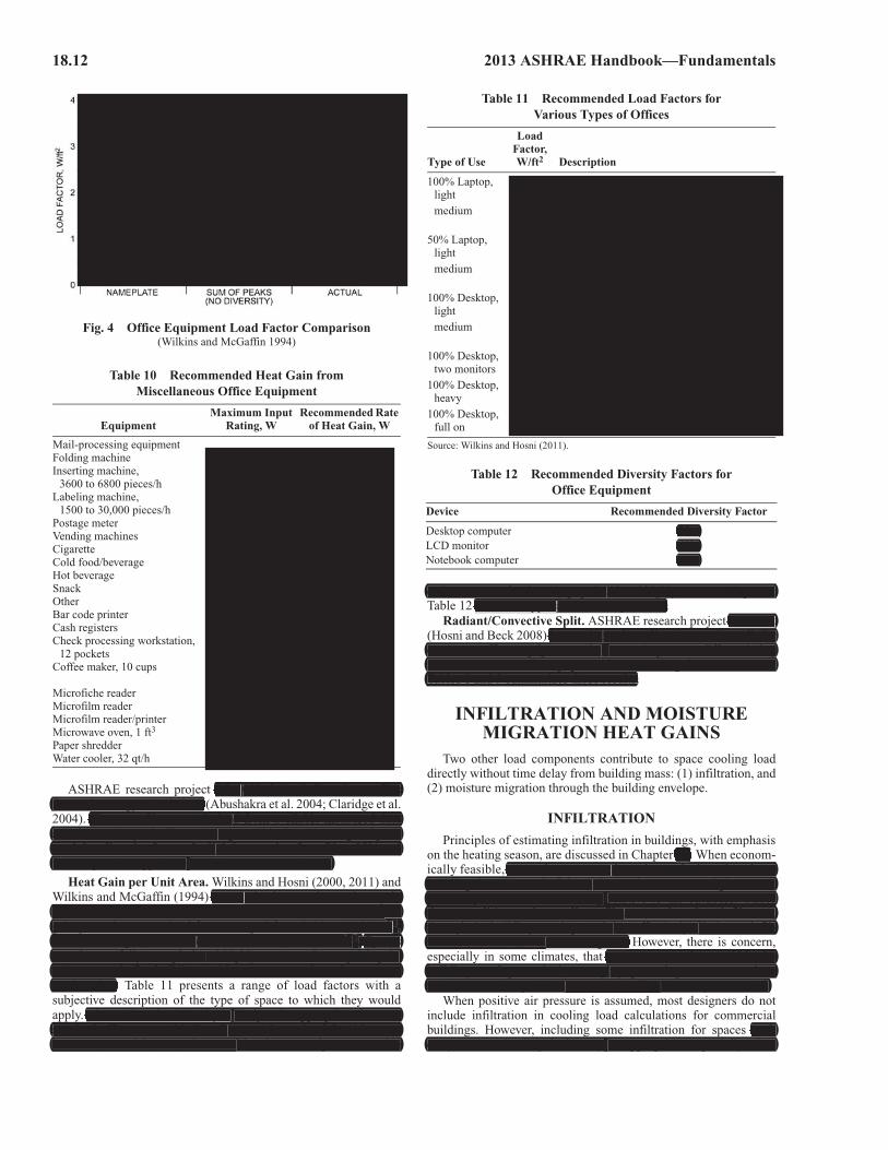
18.12 2013 ASHRAE Handbook—Fundamentals
ASHRAE research project RP-1093 derived diversity profilesfor use in energy calculations (Abushakra et al. 2004; Claridge et al.2004). Those profiles were derived from available measured datasets for a variety of office buildings, and indicated a range of peakweekday diversity factors for lighting ranging from 70 to 85% andfor receptacles (appliance load) between 42 and 89%.
Heat Gain per Unit Area. Wilkins and Hosni (2000, 2011) andWilkins and McGaffin (1994) summarized research on a heat gainper unit area basis. Diversity testing showed that the actual heatgain per unit area, or load factor, ranged from 0.44 to 1.08 W/ft2,with an average (normalized based on area) of 0.81 W/ft2. Spacestested were fully occupied and highly automated, comprising 21unique areas in five buildings, with a computer and monitor at everyworkstation. Table 11 presents a range of load factors with asubjective description of the type of space to which they wouldapply. The medium load density is likely to be appropriate for moststandard office spaces. Medium/heavy or heavy load densities maybe encountered but can be considered extremely conservative
estimates even for densely populated and highly automated spaces.Table 12 indicates applicable diversity factors.
Radiant/Convective Split. ASHRAE research project RP-1482(Hosni and Beck 2008) is examining the radiant/convective split forcommon office equipment; the most important differentiatingfeature is whether the equipment had a cooling fan. Footnotes inTables 8 and 9 summarizes those results.
INFILTRATION AND MOISTURE MIGRATION HEAT GAINS
Two other load components contribute to space cooling loaddirectly without time delay from building mass: (1) infiltration, and(2) moisture migration through the building envelope.
INFILTRATION
Principles of estimating infiltration in buildings, with emphasison the heating season, are discussed in Chapter 16. When econom-ically feasible, somewhat more outdoor air may be introduced to abuilding than the total of that exhausted, to create a slight overallpositive pressure in the building relative to the outdoors. Underthese conditions, air usually exfiltrates, rather than infiltrates,through the building envelope and thus effectively eliminates infil-tration sensible and latent heat gains. However, there is concern,especially in some climates, that water may condense within thebuilding envelope; actively managing space air pressures to reducethis condensation problem, as well as infiltration, may be needed.
When positive air pressure is assumed, most designers do notinclude infiltration in cooling load calculations for commercialbuildings. However, including some infiltration for spaces suchentry areas or loading docks may be appropriate, especially when
Table 10 Recommended Heat Gain from Miscellaneous Office Equipment
EquipmentMaximum Input
Rating, WRecommended Rate
of Heat Gain, W
Mail-processing equipmentFolding machine 125 80Inserting machine,
3600 to 6800 pieces/h600 to 3300 390 to 2150
Labeling machine,1500 to 30,000 pieces/h
600 to 6600 390 to 4300
Postage meter 230 150Vending machinesCigarette 72 72Cold food/beverage 1150 to 1920 575 to 960Hot beverage 1725 862Snack 240 to 275 240 to 275OtherBar code printer 440 370Cash registers 60 48Check processing workstation,
12 pockets4800 2470
Coffee maker, 10 cups 1500 1050 W sens., 1540 Btu/h latent
Microfiche reader 85 85Microfilm reader 520 520Microfilm reader/printer 1150 1150Microwave oven, 1 ft3 600 400Paper shredder 250 to 3000 200 to 2420Water cooler, 32 qt/h 700 350
Fig. 4 Office Equipment Load Factor Comparison(Wilkins and McGaffin 1994)
Table 11 Recommended Load Factors for Various Types of Offices
Type of Use
Load Factor,W/ft2 Description
100% Laptop, light
0.25 167 ft2/workstation, all laptop use, 1 printer per 10, speakers, misc.
medium 0.33 125 ft2/workstation, all laptop use, 1 printer per 10, speakers, misc.
50% Laptop, light
0.40 167 ft2/workstation, 50% laptop / 50% desk-top, 1 printer per 10, speakers, misc.
medium 0.50 125 ft2/workstation, 50% laptop / 50% desk-top, 1 printer per 10, speakers, misc.
100% Desktop, light
0.60 167 ft2/workstation, all desktop use, 1 printer per 10, speakers, misc.
medium 0.80 125 ft2/workstation, all desktop use, 1 printer per 10, speakers, misc.
100% Desktop, two monitors
1.00 125 ft2/workstation, all desktop use, 2 moni-tors, 1 printer per 10, speakers, misc.
100% Desktop, heavy
1.50 85 ft2/workstation, all desktop use, 2 monitors, 1 printer per 8, speakers, misc.
100% Desktop, full on
2.00 85 ft2/workstation, all desktop use, 2 monitors, 1 printer per 8, speakers, misc., no diversity.
Source: Wilkins and Hosni (2011).
Table 12 Recommended Diversity Factors for Office Equipment
Device Recommended Diversity Factor
Desktop computer 75%LCD monitor 60%Notebook computer 75%
summarized research on a heat gainper unit area basis. Diversity testing showed that the actual heat
ft2,gain per unit area, or load factor, ranged from 0.44 to 1.08 W/fft2. with an average (normalized based on area) of 0.81 W/f Spaces
tested were fully occupied and highly automated, comprising 21unique areas in five buildings, with a computer and monitor at everyworkstation.
RP-1093 derived diversity profilesfor use in energy calculations (
Those profiles were derived from available measured datasets for a variety of office buildings, and indicated a range of peakweekday diversity factors for lighting ranging from 70 to 85% andfor receptacles (appliance load) between 42 and 89%.
indicates applicable diversity factors.estimates even for densely populated and highly automated spaces.
The medium load density is likely to be appropriate for moststandard office spaces. Medium/heavy or heavy load densities maybe encountered but can be considered extremely conservative
t RP-1482) is examining the radiant/convective split for
common office equipment; the most important differentiatingfeature is whether the equipment had a cooling fan. Footnotes inTables 8 and 9 summarizes those results.
r 16. somewhat more outdoor air may be introduced to a
building than the total of that exhausted, to create a slight overallpositive pressure in the building relative to the outdoors. Underthese conditions, air usually exfiltrates, rather than infiltrates,through the building envelope and thus effectively eliminates infil-tration sensible and latent heat gains.
water may condense within thebuilding envelope; actively managing space air pressures to reducethis condensation problem, as well as infiltration, may be needed.
suchentry areas or loading docks may be appropriate, especially when
75%60%75%
Nonresidential Cooling and Heating Load Calculations 18.13
those spaces are on the windward side of buildings. But the down-ward stack effect, as occurs when indoor air is denser than the out-door, might eliminate infiltration to these entries on lower floors oftall buildings; infiltration may occur on the upper floors duringcooling conditions if makeup air is not sufficient.
Infiltration also depends on wind direction and magnitude, tem-perature differences, construction type and quality, and occupantuse of exterior doors and operable windows. As such, it is impossi-ble to accurately predict infiltration rates. Designers usually predictoverall rates of infiltration using the number of air changes perhour (ACH). A common guideline for climates and buildings typ-ical of at least the central United States is to estimate the ACHs forwinter heating conditions, and then use half that value for the cool-ing load calculations.
Standard Air VolumesBecause the specific volume of air varies appreciably, calcula-
tions are more accurate when made on the basis of air mass insteadof volume. However, volumetric flow rates are often required forselecting coils, fans, ducts, etc.; basing volumes on measurement atstandard conditions may be used for accurate results. One standardvalue is 0.075 lbda/ft3 (13.33 ft3/lb). This density corresponds toabout 60°F at saturation and 69°F dry air (at 14.696 psia). Becauseair usually passes through the equipment at a density close to stan-dard for locations below about 1000 ft, the accuracy desired nor-mally requires no correction. When airflow is to be measured at aparticular condition or point, such as at a coil entrance or exit, thecorresponding specific volume can be read from the sea-levelpsychrometric chart. For higher elevations, the mass flow rates ofair must be adjusted and higher-elevation psychrometric charts oralgorithms must be used.
Heat Gain Calculations Using Standard Air ValuesAir-conditioning design often requires the following infor-
mation:
1. Total heatTotal heat gain qt corresponding to the change of a given standard
flow rate Qs through an enthalpy difference h is
qt = 60 0.075Qsh = 4.5Qsh (8)
where 60 = min/h, 0.075 = lbda/ft3.This total heat equation can also be expressed as
qt = Ct Qsh
where Ct = 4.5 is the air total heat factor, in Btu/h·cfm per Btu/lbenthalpy h.
2. Sensible heatSensible heat gain qs corresponding to the change of dry-bulb
temperature t for given airflow (standard conditions) Qs is
qs = 60 0.075(0.24 + 0.45W )Qst (9)
where0.24 = specific heat of dry air, Btu/lb·°F
W = humidity ratio, lbw /lbda0.45 = specific heat of water vapor, Btu/lb·°F
The specific heats are for a range from about –100 to 200°F.When W = 0, the value of 60 0.075 (0.24 + 0.45W) = 1.08; whenW = 0.01, the value is 1.10; when W = 0.02, the value is 1.12; andwhen W = 0.03, the value is 1.14. Because a value of W = 0.01approximates conditions found in many air-conditioning problems,the sensible heat change (in Btu/h) has traditionally been found as
qs = 1.10Qst (10)
This sensible heat equation can also be expressed as
qs = Cs Qst
where Cs = 1.1 is the air sensible heat factor, in Btu/h·cfm·°F.
3. Latent heatLatent heat gain ql corresponding to the change of humidity ratio
W (in lbm,w/lbm,da) for given airflow (standard conditions) Qs is
ql = 60 0.075 1076QsW = 4840QsW (11)
where 1076 Btu/lb is the approximate heat content of 50% rh vaporat 75°F less the heat content of water at 50°F. A common designcondition for the space is 50% rh at 75°F, and 50°F is normal con-densate temperature from cooling and dehumidifying coils.
This latent heat equation can also be expressed as
ql = Cl QsW
where Cl = 4840 is the air latent heat factor, in Btu/h·cfm. When Wis in grw /lbm,da, Cl = 0.69 Btu/h·cfm.
4. Elevation correction for total, sensible, and latent heat equationsThe constants 4.5, 1.10, and 4840 are useful in air-conditioning
calculations at sea level (14.696 psia) and for normal temperaturesand moisture ratios. For other conditions, more precise valuesshould be used. For an elevation of 5000 ft (12.2 psia), appropriatevalues are 3.74, 0.92, and 4027. Equations (9) to (11) can becorrected for elevations other than sea level by multiplying them bythe ratio of pressure at sea level divided by the pressure at actual alti-tude. This can be derived from Equation (3) in Chapter 1 as
Cx,alt = Cx,0P/P0
where Cx,0 is any of the sea-level C values and P/P0 = [1 – (elevation 6.8754 10–6)]5.2559, where elevation is in feet.
Elevation Correction ExamplesTo correct the C values for El Paso, Texas, the elevation listed in
the appendix of Chapter 14 is 3917 ft. C values for Equations (8) to(11) can be corrected using Equation (3) in Chapter 1 as follows:
Ct,3917 = 4.5 × [1 – (3917 × 6.8754 × 10–6)]5.2559 = 3.90
Cs,3917 = 1.10 × [1 – (3917 × 6.8754 × 10–6)]5.2559 = 0.95
Cl,3917 = 4840 × [1 – (3917 × 6.8754 × 10–6)]5.2559 = 4192
To correct the C values for Albuquerque, New Mexico, the ele-vation listed in the appendix of Chapter 14 is 5315 ft. C values forEquations (8) to (11) can be corrected as follows:
Ct,5315 = 4.5 × [1 – (5315 × 6.8754 × 10–6)]5.2559 Ct,531 = 3.70
Cs,5315 = 1.10 × [1 – (5315 × 6.8754 × 10–6)]5.2559 Cs,5315 = 0.90
Cl,5315 = 4840 × [1 – (5315 × 6.8754 × 10–6)]5.2559 Cl,5315 = 3979
LATENT HEAT GAIN FROM MOISTURE DIFFUSION
Diffusion of moisture through building materials is a natural phe-nomenon that is always present. Chapters 25 to 27 cover principles,materials, and specific methods used to control moisture. Moisturetransfer through walls and roofs is often neglected in comfort airconditioning because the actual rate is quite small and the corre-sponding latent heat gain is insignificant. Permeability and per-meance values for various building materials are given in Chapter26. Vapor retarders should be specified and installed in the properlocation to keep moisture transfer to a minimum, and to minimizecondensation within the envelope. Moisture migration up through
those spaces are on the windward side of buildings. But the down-ward stack effect, as occurs when indoor air is denser than the out-door, might eliminate infiltration to these entries on lower floors oftall buildings; infiltration may occur on the upper floors duringcooling conditions if makeup air is not sufficient.
on wind direction and magnitude, tem-perature differences, construction type and quality, and occupantuse of exterior doors and operable windows. As such, it is impossi-ble to accurately predict infiltration rates. D
typ-ical of at least the central United States is to estimate the ACHs forwinter heating conditions, and then use half that value for the cool-ing load calculations.
more accurate when made on the basis of air mass insteadof volume. However, volumetric flow rates are often required forselecting coils, fans, ducts, etc.; basing volumes on measurement atstandard conditions may be used for accurate results.
ft3 ft3/0.075 lbda/f (13.33 /lb). This density corresponds todaabout 60°F at saturation and 69°F dry air (at 14.696 psia). Becauserrair usually passes through the equipment at a density close to stan-dard for locations below about 1000 ft, the accuracy desired nor-mally requires no correction.
can be read from the sea-levelpsychrometric chart. For higher elevations, the mass flow rates ofair must be adjusted and higher-elevation psychrometric charts oralgorithms must be used.
qt t = 60 0.075QsQsh = 4.5QsQsh
ft3.60 = min/h, 0.075 = lbda/f
qt t = CtCC Qssh
CtC t = 4.5
qs = 60 0.075(0.24 + 0.45W ))QsQst (9)
where0.24 = specific heat of dry air, Btu/lb·°F
W = humidity ratio, lbw /lbdaw da0.45 = specific heat of water vapor, Btu/lb·°F
The specific heats are for a range from about –100 to 200°F.When W = 0, the value of 60W 0.075 (0.24 + 0.45W) = 1.08; whenWWW = 0.01, the value is 1.10; when W = 0.02, the value is 1.12; andWwhen W = 0.03, the value is 1.14. Because a value of W W = 0.01Wapproximates conditions found in many air-conditioning problems,the sensible heat change (in Btu/h) has traditionally been found as
qs = 1.10Qsst
qs = CsC QsQst
where CsC = 1.1 is the air sensible heat factor, in Btu/h·cfm·°F.
W ((in n lbm,w/lbm,da) lfor given airflow (standard conditions) QsQ is
ql = 60 0.075 1076QsQsW W = 4840QsQsW (11)
1076 Btu/lb is the approximate heat content of 50% rh vaporat 75°F less the heat content of water at 50°F. A common designfcondition for the space is 50% rh at 75°F, and 50°F is normal con-densate temperature from cooling and dehumidifying coils.
ql l = ClC QsQsW
where e ClC ll = 4840 is the air latent heat l factor, in Btu/h·cfm. When Wis in
ln grw /lbm,da, ClC l = 0.69 Btu/h·cfm.
4.5, 1.10, and 4840 are useful in air-conditioningcalculations at sea level (14.696 psia) and for normal temperaturesand moisture ratios. For other conditions, more precise valuesshould be used. For an elevation of 5000 ft (12.2 psia), appropriatefvalues are 3.74, 0.92, and 4027. Equations (9) to (11) can becorrected for elevations other than sea level by multiplying them bythe ratio of pressure at sea level divided by the pressure at actual alti-tude. This can be derived from Equation (3) in Chapter 1 as
CxCC , = CxCC ,0P/PP P// 0,alt t
where e CxCC , is any of the sea-level C values and C P/PP/P// 0 = [1 – (elevation,0 5.2559,
x 6.8754
, 10–6)]5
0where elevation is in feet.
25 to 27
26. specified and installed in the properlocation to keep moisture transfer to a minimum, and to minimizecondensation within the envelope. up through

18.14 2013 ASHRAE Handbook—Fundamentals
slabs-on-grade and basement floors has been found to be signifi-cant, but has historically not been addressed in cooling load calcu-lations. Under-slab continuous moisture retarders and drainage canreduce upward moisture flow.
Some industrial applications require low moisture to be main-tained in a conditioned space. In these cases, the latent heat gainaccompanying moisture transfer through walls and roofs may begreater than any other latent heat gain. This gain is computed by
= (M/7000)Apv (hg –hf) (12)
where= latent heat gain from moisture transfer, Btu/h
M = permeance of wall or roof assembly, perms or grains/(ft2·h·in. Hg)
7000 = grains/lbA = area of wall or roof surface, ft2
pv = vapor pressure difference, in. Hghg = enthalpy at room conditions, Btu/lbhf = enthalpy of water condensed at cooling coil, Btu/lb
hg – hf = 1076 Btu/lb when room temperature is 75°F and condensate off coil is 50°F
OTHER LATENT LOADS
Moisture sources within a building (e.g., shower areas, swim-ming pools or natatoriums, arboretums) can also contribute to latentload. Unlike sensible loads, which correlate to supply air quantitiesrequired in a space, latent loads usually only affect cooling coils siz-ing or refrigeration load. Because air from showers and some othermoisture-generating areas is exhausted completely, those airbornelatent loads do not reach the cooling coil and thus do not contributeto cooling load. However, system loads associated with ventilationair required to make up exhaust air must be recognized, and anyrecirculated air’s moisture must be considered when sizing thedehumidification equipment.
For natatoriums, occupant comfort and humidity control are crit-ical. In many instances, size, location, and environmental require-ments make complete exhaust systems expensive and ineffective.Where recirculating mechanical cooling systems are used, evapora-tion (latent) loads are significant. Chapter 5 of the 2011 ASHRAEHandbook—HVAC Applications provides guidance on natatoriumload calculations.
FENESTRATION HEAT GAINFor spaces with neutral or positive air pressurization, the primary
weather-related variable affecting cooling load is solar radiation.The effect of solar radiation is more pronounced and immediate onexposed, nonopaque surfaces. Chapter 14 includes procedures forcalculating clear-sky solar radiation intensity and incidence anglesfor weather conditions encountered at specific locations. That chap-ter also includes some useful solar equations. Calculation of solarheat gain and conductive heat transfer through various glazingmaterials and associated mounting frames, with or without interiorand/or exterior shading devices, is discussed in Chapter 15. Thischapter covers application of such data to overall heat gain evalua-tion, and conversion of calculated heat gain into a composite cool-ing load for the conditioned space.
FENESTRATION DIRECT SOLAR, DIFFUSE SOLAR, AND CONDUCTIVE HEAT GAINS
For fenestration heat gain, use the following equations:
Direct beam solar heat gain qb:
qb = AEt,b SHGC(�)IAC(�,�) (13)
Diffuse solar heat gain qd:
qd = A(Et,d + Et,r) SHGC�D IACD (14)
Conductive heat gain qc:
qc = UA(Tout – Tin) (15)
Total fenestration heat gain Q:
Q = qb + qd + qc (16)
whereA = window area, ft2
Et,b, Et,d,and Et,r = beam, sky diffuse, and ground-reflected diffuse irradiance,
calculated using equations in Chapter 14SHGC(�) = beam solar heat gain coefficient as a function of incident
angle �; may be interpolated between values in Table 10 of Chapter 15
SHGC�D = diffuse solar heat gain coefficient (also referred to as hemispherical SHGC); from Table 10 of Chapter 15
Tin = indoor temperature, °FTout = outdoor temperature, °F
U = overall U-factor, including frame and mounting orientation from Table 4 of Chapter 15, Btu/h·ft2·°F
IAC(�.�) = indoor solar attenuation coefficient for beam solar heat gain coefficient; = 1.0 if no indoor shading device. IAC(�.�) is a function of shade type and, depending on type, may also be a function of beam solar angle of incidence � and shade geometry
IACD = indoor solar attenuation coefficient for diffuse solar heat gain coefficient; = 1.0 if not indoor shading device. IACD is a function of shade type and, depending on type, may also be a function of shade geometry
If specific window manufacturer’s SHGC and U-factor data areavailable, those should be used. For fenestration equipped withindoor shading (blinds, drapes, or shades), the indoor solar attenu-ation coefficients IAC(�.�) and IACD are listed in Tables 13A to13G of Chapter 15.
Note that, as discussed in Chapter 15, fenestration ratings (U-factor and SHGC) are based on the entire product area, includingframes. Thus, for load calculations, fenestration area is the area ofthe entire opening in the wall or roof.
EXTERIOR SHADING
Nonuniform exterior shading, caused by roof overhangs, sidefins, or building projections, requires separate hourly calculationsfor the externally shaded and unshaded areas of the window in ques-tion, with the indoor shading SHGC still used to account for anyinternal shading devices. The areas, shaded and unshaded, dependon the location of the shadow line on a surface in the plane of theglass. Sun (1968) developed fundamental algorithms for analysis ofshade patterns. McQuiston and Spitler (1992) provide graphicaldata to facilitate shadow line calculation.
Equations for calculating shade angles [Chapter 15, Equations(34) to (37)] can be used to determine the shape and area of a mov-ing shadow falling across a given window from external shadingelements during the course of a design day. Thus, a subprofile ofheat gain for that window can be created by separating its sunlit andshaded areas for each hour.
HEAT BALANCE METHODCooling load estimation involves calculating a surface-by-
surface conductive, convective, and radiative heat balance for eachroom surface and a convective heat balance for the room air. Theseprinciples form the foundation for all methods described in thischapter. The heat balance (HB) method solves the problem directly
ql m
ql m
slabs-on-grade and basement floors has been found to be signifi-cant, but has historically not been addressed in cooling load calcu-nlations. canreduce upward moisture flow.
where= latent heat gain from moisture transfer, Btu/h
M = permeance of wall or roof assembly, perms or m
ft2grains/(f 2·h·in. Hg)7000 = grains/lb
ft2A = area of wall or roof surface, p v = vapor pressure difference, in. Hg
hg = enthalpy at room conditions, Btu/lbghfh = enthalpy of water condensed at cooling coil, Btu/lb
hg g – f
hfh = 1076 Btu/lb when room temperature is 75°F and condensate off coil is 50°F
= (M(( /7000)MM A)) p v ((hg g ––hfh )ff (12)qll m
can also contribute to latentload. correlate to supply air quantitiesrequired in a space, latent loads usually only affect cooling coils siz-ing or refrigeration load. Because air from showers and some othermoisture-generating areas is exhausted completely, those airbornelatent loads do not reach the cooling coil and thus do not contributeto cooling load. ventilationair required to make up exhaust air must be recognized, and anyrecirculated air’s moisture must be considered when sizing thedehumidification equipment.
e crit-ical. In many instances, size, location, and environmental require-ments make complete exhaust systems expensive and ineffective.Where recirculating mechanical cooling systems are used, evapora-tion (latent) loads are significant. 5 2011 ASHRAEHandbook—HVAC Applications provides guidance on natatoriumload calculations.
more pronounced and immediate onexposed, nonopaque surfaces. 14 procedures forcalculating clear-sky solar radiation intensity and incidence anglesfor weather conditions encountered at specific locations. That chap-tter also includes some useful solar equations. Calculation of solarheat gain and conductive heat transfer through various glazingmaterials and associated mounting frames, with or without interiorand/or exterior shading devices, is 15.
application of such data to overall heat gain evalua-tion, and conversion of calculated heat gain into a composite cool-ing load for the conditioned space.
Direct beam solar heat gain qb:
qb = AEt, SHGC(��)IAC(��,��) (13),b
Diffuse solar heat gain qd:
�qd d = A((E(( t, + Et,r) SHGC� IACD (14),d �D
Conductive heat gain qc:
qc = UA((Tout TT t – TinTT ) (15)
Total fenestration heat gain Q:
Q = qb + qd d + qc (16)
whereft2A = window area,
Et,b, Et,d,t,band
,Et, = beam, sky diffuse, and ground-reflected diffuse irradiance,,r
calculated using equations in Chapter 14SHGC(��) = beam solar heat gain coefficient as a function of incident
angle ��; may be interpolated between values in Table 10 of Chapter 15
� SHGC� = diffuse solar heat gain coefficient (also referred to as ff�D hemispherical SHGC); from Table 10 of Chapter 15
TinTT = indoor temperature, °FTout TT = outdoor temperature, °F
U = overall U-factor, including frame and mounting orientation ft2from Table 4 of Chapter 15, Btu/h·f 2·°F
IAC(��.��) = indoor solar attenuation coefficient for beam solar heat gaincoefficient; = 1.0 if no indoor shading device. IAC(�.�) is afunction of shade type and, depending on type, may also be afunction of beam solar angle of incidence � and shadegeometry
IACD = indoor solar attenuation coefficient for diffuse solar heat gain coefficient; = 1.0 if not indoor shading device. IACD is a function of shade type and, depending on type, may also be afunction of shade geometry
IAC(��.��) and IACD r 15.
15, (U-factor and SHGC)
ofthe entire opening in the wall or roof.
requires separate hourly calculationsfor the externally shaded and unshaded areas of the window in ques-tion, with the indoor shading SHGC still used to account for anyinternal shading devices.
d fundamental algorithms for analysis ofshade patterns. provide graphicaldata to facilitate shadow line calculation.
determine the shape and area of a mov-ing shadow falling across a given window from external shadingelements during the course of a design day. Thus, a subprofile ofheat gain for that window can be created by separating its sunlit andshaded areas for each hour.

Nonresidential Cooling and Heating Load Calculations 18.15
instead of introducing transformation-based procedures. The ad-vantages are that it contains no arbitrarily set parameters, and noprocesses are hidden from view.
Some computations required by this rigorous approach requirethe use of computers. The heat balance procedure is not new. Manyenergy calculation programs have used it in some form for manyyears. The first implementation that incorporated all the elements toform a complete method was NBSLD (Kusuda 1967). The heatbalance procedure is also implemented in both the BLAST andTARP energy analysis programs (Walton 1983). Before ASHRAEresearch project RP-875, the method had never been described com-pletely or in a form applicable to cooling load calculations. Thepapers resulting from RP-875 describe the heat balance procedurein detail (Liesen and Pedersen 1997; McClellan and Pedersen 1997;Pedersen et al. 1997).
The HB method is codified in the software called Hbfort thataccompanies Cooling and Heating Load Calculation Principles(Pedersen et al. 1998).
ASHRAE research project RP-1117 constructed two modelrooms for which cooling loads were physically measured usingextensive instrumentation (Chantrasrisalai et al. 2003; Eldridgeet al. 2003; Iu et al. 2003). HB calculations closely approximatedmeasured cooling loads when provided with detailed data for thetest rooms.
ASSUMPTIONS
All calculation procedures involve some kind of model; all mod-els require simplifying assumptions and, therefore, are approxi-mate. The most fundamental assumption is that air in the thermalzone can be modeled as well mixed, meaning its temperature isuniform throughout the zone. ASHRAE research project RP-664(Fisher and Pedersen 1997) established that this assumption is validover a wide range of conditions.
The next major assumption is that the surfaces of the room(walls, windows, floor, etc.) can be treated as having
• Uniform surface temperatures• Uniform long-wave (LW) and short-wave (SW) irradiation• Diffuse radiating surfaces• One-dimensional heat conduction within
The resulting formulation is called the heat balance (HB)model. Note that the assumptions, although common, are quiterestrictive and set certain limits on the information that can beobtained from the model.
ELEMENTS
Within the framework of the assumptions, the HB can be viewedas four distinct processes:
1. Outdoor-face heat balance2. Wall conduction process3. Indoor-face heat balance4. Air heat balance
Figure 5 shows the relationship between these processes for asingle opaque surface. The top part of the figure, inside the shadedbox, is repeated for each surface enclosing the zone. The process fortransparent surfaces is similar, but the absorbed solar componentappears in the conduction process block instead of at the outdoorface, and the absorbed component splits into inward- and outward-flowing fractions. These components participate in the surface heatbalances.
Outdoor-Face Heat BalanceThe heat balance on the outdoor face of each surface is
q��sol + q�LWR + q�conv – q�ko = 0 (17)
whereq��sol = absorbed direct and diffuse solar radiation flux (q/A), Btu/h·ft2
q�LWR = net long-wave radiation flux exchange with air and surroundings, Btu/h·ft2
q�conv = convective exchange flux with outdoor air, Btu/h·ft2
q�ko = conductive flux (q/A) into wall, Btu/h·ft2
All terms are positive for net flux to the face except q�ko, which istraditionally taken to be positive from outdoors to inside the wall.
Each term in Equation (17) has been modeled in several ways,and in simplified methods the first three terms are combined byusing the sol-air temperature.
Wall Conduction ProcessThe wall conduction process has been formulated in more ways
than any of the other processes. Techniques include
• Numerical finite difference• Numerical finite element• Transform methods• Time series methods
This process introduces part of the time dependence inherent inload calculation. Figure 6 shows surface temperatures on the indoorand outdoor faces of the wall element, and corresponding conduc-tive heat fluxes away from the outer face and toward the indoor face.All four quantities are functions of time. Direct formulation of theprocess uses temperature functions as input or known quantities,and heat fluxes as outputs or resultant quantities.
In some models, surface heat transfer coefficients are included aspart of the wall element, making the temperatures in question the
Fig. 5 Schematic of Heat Balance Processes in Zone
that it contains no arbitrarily set parameters, and noprocesses are hidden from view.
called Hbfort thataccompanies Cooling and Heating Load Calculation Principles(Pedersen et al. 1998).
RP-1117 constructed two modelrooms for which cooling loads were physically measured usingextensive instrumentation (Chantrasrisalai et al. 2003; Eldridgeet al. 2003; Iu et al. 2003). closely approximatedmeasured cooling loads when provided with detailed data for thetest rooms.
NBSLD (Kusuda 1967). implemented in both the BLAST and
TARP energy analysis programs (Walton 1983). t RP-875, the method had never been described com-
pletely or in a form applicable to cooling load calculations. Thepapers resulting from RP-875 describe the heat balance procedurein detail (Liesen and Pedersen 1997; McClellan and Pedersen 1997;Pedersen et al. 1997).
well mixed, meaning its temperature isuniform throughout the zone. RP-664(Fisher and Pedersen 1997)
The next major assumption is that the surfaces of the room(walls, windows, floor, etc.) can be treated as having
• Uniform surface temperatures• Uniform long-wave (LW) and short-wave (SW) irradiation• Diffuse radiating surfaces• One-dimensional heat conduction within
the heat balance (HB)model.
four distinct p
1. Outdoor-face heat balance2. Wall conduction process3. Indoor-face heat balance4. Air heat balance
similar, but the absorbed solar componentappears in the conduction process block instead of at the outdoorface, and the absorbed component splits into inward- and outward-flowing fractions. These components participate in the surface heatbalances.
q� + q� + q� – q� = 0 (17)q�sol qLWR qconv qko
whereft2q� = absorbed direct and diffuse solar radiation flux (q/A), Btu/h·fq�sol l
q� = net long-wave radiation flux exchange with air and qLWR ft2surroundings, Btu/h·f
ft2q� = convective exchange flux with outdoor air, Btu/h·fqconv vft2q� = conductive flux (q/A) into wall, Btu/h·fqko
qpositive for net flux to the face except qq�ko, which isqkotraditionally taken to be positive from outdoors to inside the wall.
simplified methods the first three terms are combined byusing the sol-air temperature.
• Numerical finite difference• Numerical finite element• Transform methods• Time series methods
part of the time dependence inherent infload calculation. F 6 shows surface temperatures on the indoorand outdoor faces of the wall element, and corresponding conduc-tive heat fluxes away from the outer face and toward the indoor face.All four quantities are functions of time.
temperature functions as input or known quantities,and heat fluxes as outputs or resultant quantities.
surface heat transfer coefficients are included aspart of the wall element, making the temperatures in question the

18.16 2013 ASHRAE Handbook—Fundamentals
indoor and outdoor air temperatures. This is not a desirable formu-lation, because it hides the heat transfer coefficients and prohibitschanging them as airflow conditions change. It also prohibits treat-ing the internal long-wave radiation exchange appropriately.
Because heat balances on both sides of the element induce boththe temperature and heat flux, the solution must deal with thissimultaneous condition. Two computational methods that have beenused widely are finite difference and conduction transfer functionmethods. Because of the computational time advantage, the conduc-tion transfer function formulation has been selected for presentationhere.
Indoor-Face Heat BalanceThe heart of the HB method is the internal heat balance involving
the inner faces of the zone surfaces. This heat balance has many heattransfer components, and they are all coupled. Both long-wave(LW) and short-wave (SW) radiation are important, as well as wallconduction and convection to the air. The indoor-face heat balancefor each surface can be written as follows:
q�LWX + q�SW + q�LWS + q�ki + q�sol + q�conv = 0 (18)
whereq�LWX = net long-wave radiant flux exchange between zone surfaces,
Btu/h·ft2
q�SW = net short-wave radiation flux to surface from lights, Btu/h·ft2
q�LWS = long-wave radiation flux from equipment in zone, Btu/h·ft2
q�ki = conductive flux through wall, Btu/h·ft2
q�sol = transmitted solar radiative flux absorbed at surface, Btu/h·ft2
q�conv = convective heat flux to zone air, Btu/h·ft2
These terms are explained in the following paragraphs.LW Radiation Exchange Among Zone Surfaces. The limiting
cases for modeling internal LW radiation exchange are
• Zone air is completely transparent to LW radiation• Zone air completely absorbs LW radiation from surfaces in the
zone
Most HB models treat air as completely transparent and not par-ticipating in LW radiation exchange among surfaces in the zone.The second model is attractive because it can be formulated simplyusing a combined radiative and convective heat transfer coefficientfrom each surface to the zone air and thus decouples radiantexchange among surfaces in the zone. However, because the trans-parent air model allows radiant exchange and is more realistic, thesecond model is inferior.
Furniture in a zone increases the amount of surface area that canparticipate in radiative and convective heat exchanges. It also adds
thermal mass to the zone. These two changes can affect the timeresponse of the zone cooling load.
SW Radiation from Lights. The short-wavelength radiationfrom lights is usually assumed to be distributed over the surfaces inthe zone in some manner. The HB procedure retains this approachbut allows the distribution function to be changed.
LW Radiation from Internal Sources. The traditional modelfor this source defines a radiative/convective split for heat intro-duced into a zone from equipment. The radiative part is then distrib-uted over the zone’s surfaces in some manner. This model is notcompletely realistic, and it departs from HB principles. In a true HBmodel, equipment surfaces are treated just as other LW radiantsources within the zone. However, because information about thesurface temperature of equipment is rarely known, it is reasonable tokeep the radiative/convective split concept even though it ignoresthe true nature of the radiant exchange. ASHRAE research projectRP-1055 (Hosni et al. 1999) determined radiative/convective splitsfor many additional equipment types, as listed in footnotes forTables 8 and 9.
Transmitted Solar Heat Gain. Chapter 15’s calculation proce-dure for determining transmitted solar energy through fenestrationuses the solar heat gain coefficient (SHGC) directly rather thanrelating it to double-strength glass, as is done when using a shadingcoefficient (SC). The difficulty with this plan is that the SHGCincludes both transmitted solar and inward-flowing fraction of thesolar radiation absorbed in the window. With the HB method, thislatter part should be added to the conduction component so it can beincluded in the indoor-face heat balance.
Transmitted solar radiation is also distributed over surfaces in thezone in a prescribed manner. It is possible to calculate the actualposition of beam solar radiation, but this involves partial surfaceirradiation, which is inconsistent with the rest of the zone model,which assumes uniform conditions over an entire surface.
Using SHGC to Calculate Solar Heat GainThe total solar heat gain through fenestration consists of directly
transmitted solar radiation plus the inward-flowing fraction of solarradiation that is absorbed in the glazing system. Both parts containbeam and diffuse contributions. Transmitted radiation goes directlyonto surfaces in the zone and is accounted for in the surface indoorheat balance. The zone heat balance model accommodates theresulting heat fluxes without difficulty. The second part, the inward-flowing fraction of the absorbed solar radiation, interacts with othersurfaces of the enclosure through long-wave radiant exchange andwith zone air through convective heat transfer. As such, it dependsboth on geometric and radiative properties of the zone enclosure andconvection characteristics inside and outside the zone. The solarheat gain coefficient (SHGC) combines the transmitted solar radia-tion and the inward-flowing fraction of the absorbed radiation. TheSHGC is defined as
SHGC = � + �k (19)
where� = solar transmittance of glazing�k = solar absorptance of the kth layer of the glazing systemn = number of layers
Nk = inward-flowing fraction of absorbed radiation in the kth layer
Note that Equation (19) is written generically. It can be written fora specific incidence angle and/or radiation wavelength and inte-grated over the wavelength and/or angle, but the principle is thesame in each case. Refer to Chapter 15 for the specific expressions.
Unfortunately, the inward-flowing fraction N interacts with thezone in many ways. This interaction can be expressed as
Fig. 6 Schematic of Wall Conduction Process
Nkk=1
n
�
indoor and outdoor air temperatures. This is not a desirable formu-lation, because it hides the heat transfer coefficients and prohibitschanging them as airflow conditions change. It also prohibits treat-ing the internal long-wave radiation exchange appropriately.
induce boththe temperature and heat flux, the solution must deal with thissimultaneous condition. Two computational methods that have beenused widely are finite difference and conduction transfer functionmethods. Because of the computational time advantage, the conduc-tion transfer function formulation has been selected for presentationhere.
internal heat balance involvingthe inner faces of the zone surfaces. This heat balance has many heattransfer components, and they are all coupled. Both long-wave(LW) and short-wave (SW) radiation are important, as well as wallconduction and convection to the air.
q� + q� + q� + q� + q� + q� = 0 (18)qLWX qSW qLWS qki qsol qconv
whereq� = net long-wave radiant flux exchange between zone surfaces,qLWX g
ft2Btu/h·fft2q� = net short-wave radiation flux to surface from lights, Btu/h·fqSW
ft2q� = long-wave radiation flux from equipment in zone, Btu/h·fqLWSft2q� = conductive flux through wall, Btu/h·fqki
ft2q� = transmitted solar radiative flux absorbed at surface, Btu/h·fqsolft2q� = convective heat flux to zone air, Btu/h·fqconv
• Zone air is completely transparent to LW radiation• Zone air completely absorbs LW radiation from surfaces in the
zone
Most HB models treat air as completely transparent and not par-ticipating in LW radiation exchange among surfaces in the zone.The second model is attractive because it can be formulated simplyusing a combined radiative and convective heat transfer coefficientfrom each surface to the zone air and thus decouples radiantexchange among surfaces in the zone. trans-parent air model allows radiant exchange and is more realistic, thesecond model is inferior.
Furniture in a zone increases the amount of surface area that canparticipate in radiative and convective heat exchanges. It also adds
thermal mass to the zone. These two changes can affect the timeresponse of the zone cooling load.
The short-wavelength radiationfrom lights is usually assumed to be distributed over the surfaces inthe zone in some manner. The HB procedure retains this approachbut allows the distribution function to be changed.
The traditional modelfor this source defines a radiative/convective split for heat intro-duced into a zone from equipment. The radiative part is then distrib-uted over the zone’s surfaces in some manner. This model is notcompletely realistic, and it departs from HB principles. In a true HBmodel, equipment surfaces are treated just as other LW radiantsources within the zone. However, because information about thesurface temperature of equipment is rarely known, it is reasonable tokeep the radiative/convective split concept even though it ignoresthe true nature of the radiant exchange. RP-1055 (Hosni et al. 1999) determined radiative/convective splitsfor many additional equipment types, as listed in footnotes forTables 8 and 9.
r 15’s
solar heat gain coefficient (SHGC) directly rather thanrelating it to double-strength glass, as is done when using a shadingcoefficient (SC). The difficulty with this plan is that the SHGCincludes both transmitted solar and inward-flowing fraction of thesolar radiation absorbed in the window. With the HB method, thislatter part should be added to the conduction component so it can beincluded in the indoor-face heat balance.
s also distributed over surfaces in thezone in a prescribed manner. It is possible to calculate the actualposition of beam solar radiation, but this involves partial surfaceirradiation, which is inconsistent with the rest of the zone model,which assumes uniform conditions over an entire surface.
f directlytransmitted solar radiation plus the inward-flowing fraction of solarradiation that is absorbed in the glazing system. Both parts containbeam and diffuse contributions. Transmitted radiation goes directlyonto surfaces in the zone and is accounted for in the surface indoorheat balance. The zone heat balance model accommodates theresulting heat fluxes without difficulty. The second part, the inward-ffflowing fraction of the absorbed solar radiation, interacts with othersurfaces of the enclosure through long-wave radiant exchange andwith zone air through convective heat transfer. dependsboth on geometric and radiative properties of the zone enclosure andconvection characteristics inside and outside the zone. The solarheat gain coefficient (SHGC) combines the transmitted solar radia-tion and the inward-flowing fraction of the absorbed radiation. TheSHGC is defined as
where� = solar transmittance of glazing� = solar absorptance of the kth layer of the glazing system�kn = number of layers
NkNN = inward-flowing fraction of absorbed radiation in the kth layerkk
generically. It can be written fora specific incidence angle and/or radiation wavelength and inte-rgrated over the wavelength and/or angle, but the principle is thesame in each case. Refer to Chapter 15 for the specific expressions.
Unfortunately, the inward-flowing fraction N interacts with theNzone in many ways. This interaction can be expressed as
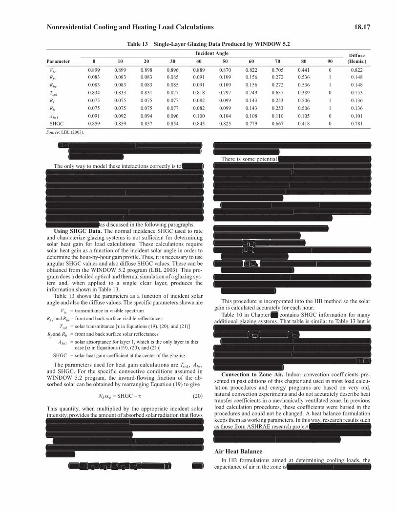
Nonresidential Cooling and Heating Load Calculations 18.17
N = f (indoor convection coefficient, outdoor convection coefficient, glazing system overall heat transfer coefficient, zone geometry, zone radiation properties)
The only way to model these interactions correctly is to combinethe window model with the zone heat balance model and solve bothsimultaneously. This has been done recently in some energy analysisprograms, but is not generally available in load calculation proce-dures. In addition, the SHGC used for rating glazing systems is basedon specific values of the indoor, outdoor, and overall heat transfercoefficients and does not include any zonal long-wavelength radia-tion considerations. So, the challenge is to devise a way to use SHGCvalues within the framework of heat balance calculation in the mostaccurate way possible, as discussed in the following paragraphs.
Using SHGC Data. The normal incidence SHGC used to rateand characterize glazing systems is not sufficient for determiningsolar heat gain for load calculations. These calculations requiresolar heat gain as a function of the incident solar angle in order todetermine the hour-by-hour gain profile. Thus, it is necessary to useangular SHGC values and also diffuse SHGC values. These can beobtained from the WINDOW 5.2 program (LBL 2003). This pro-gram does a detailed optical and thermal simulation of a glazing sys-tem and, when applied to a single clear layer, produces theinformation shown in Table 13.
Table 13 shows the parameters as a function of incident solarangle and also the diffuse values. The specific parameters shown are
Vtc = transmittance in visible spectrum
Rf v and Rbv = front and back surface visible reflectances
Tsol = solar transmittance [� in Equations (19), (20), and (21)]
Rf and Rb = front and back surface solar reflectances
Abs1 = solar absorptance for layer 1, which is the only layer in this case [� in Equations (19), (20), and (21)]
SHGC = solar heat gain coefficient at the center of the glazing
The parameters used for heat gain calculations are Tsol , Abs ,and SHGC. For the specific convective conditions assumed inWINDOW 5.2 program, the inward-flowing fraction of the ab-sorbed solar can be obtained by rearranging Equation (19) to give
Nk�k = SHGC – � (20)
This quantity, when multiplied by the appropriate incident solarintensity, provides the amount of absorbed solar radiation that flowsinward. In the heat balance formulation for zone loads, this heat fluxis combined with that caused by conduction through glazing andincluded in the surface heat balance.
The outward-flowing fraction of absorbed solar radiation is usedin the heat balance on the outdoor face of the glazing and is deter-mined from
(1 – Nk)�k = �k – Nk�k = �k – (SHGC – �) (21)
If there is more than one layer, the appropriate summation ofabsorptances must be done.
There is some potential inaccuracy in using the WINDOW 5.2SHGC values because the inward-flowing fraction part was deter-mined under specific conditions for the indoor and outdoor heattransfer coefficients. However, the program can be run with indoorand outdoor coefficients of one’s own choosing. Normally, however,this effect is not large, and only in highly absorptive glazing systemsmight cause significant error.
For solar heat gain calculations, then, it seems reasonable to usethe generic window property data that comes from WINDOW 5.2.Considering Table 13, the procedure is as follows:
1. Determine angle of incidence for the glazing.2. Determine corresponding SHGC.3. Evaluate Nk�k using Equation (19).4. Multiply Tsol by incident beam radiation intensity to get trans-
mitted beam solar radiation.5. Multiply Nk�k by incident beam radiation intensity to get
inward-flowing absorbed heat.6. Repeat steps 2 to 5 with diffuse parameters and diffuse radiation.7. Add beam and diffuse components of transmitted and inward-
flowing absorbed heat.
This procedure is incorporated into the HB method so the solargain is calculated accurately for each hour.
Table 10 in Chapter 15 contains SHGC information for manyadditional glazing systems. That table is similar to Table 13 but isslightly abbreviated. Again, the information needed for heat gaincalculations is Tsol, SHGC, and Abs.
The same caution about the indoor and outdoor heat transfercoefficients applies to the information in Table 10 in Chapter 15.Those values were also obtained with specific indoor and outdoorheat transfer coefficients, and the inward-flowing fraction N isdependent upon those values.
Convection to Zone Air. Indoor convection coefficients pre-sented in past editions of this chapter and used in most load calcu-lation procedures and energy programs are based on very old,natural convection experiments and do not accurately describe heattransfer coefficients in a mechanically ventilated zone. In previousload calculation procedures, these coefficients were buried in theprocedures and could not be changed. A heat balance formulationkeeps them as working parameters. In this way, research results suchas those from ASHRAE research project RP-664 (Fisher 1998) canbe incorporated into the procedures. It also allows determining thesensitivity of the load calculation to these parameters.
Air Heat BalanceIn HB formulations aimed at determining cooling loads, the
capacitance of air in the zone is neglected and the air heat balance is
Table 13 Single-Layer Glazing Data Produced by WINDOW 5.2
Parameter
Incident Angle Diffuse (Hemis.)0 10 20 30 40 50 60 70 80 90
Vtc 0.899 0.899 0.898 0.896 0.889 0.870 0.822 0.705 0.441 0 0.822Rfv 0.083 0.083 0.083 0.085 0.091 0.109 0.156 0.272 0.536 1 0.148
Rbv 0.083 0.083 0.083 0.085 0.091 0.109 0.156 0.272 0.536 1 0.148
Tsol 0.834 0.833 0.831 0.827 0.818 0.797 0.749 0.637 0.389 0 0.753
Rf 0.075 0.075 0.075 0.077 0.082 0.099 0.143 0.253 0.506 1 0.136
Rb 0.075 0.075 0.075 0.077 0.082 0.099 0.143 0.253 0.506 1 0.136
Abs1 0.091 0.092 0.094 0.096 0.100 0.104 0.108 0.110 0.105 0 0.101
SHGC 0.859 0.859 0.857 0.854 0.845 0.825 0.779 0.667 0.418 0 0.781
Source: LBL (2003).
N = f (indoor convection coefficient, outdoor convection coefficient,glazing system overall heat transfer coefficient, zone geometry,ffzone radiation properties)
combinethe window model with the zone heat balance model and solve bothsimultaneously. This has been done recently in some energy analysisprograms, but is not generally available in load calculation proce-dures. In addition, the SHGC used for rating glazing systems is basedon specific values of the indoor, outdoor, and overall heat transfercoefficients and does not include any zonal long-wavelength radia-tion considerations. So, the challenge is to devise a way to use SHGCvalues within the framework of heat balance calculation in the mostaccurate way possible,
inward. In the heat balance formulation for zone loads, this heat fluxis combined with that caused by conduction through glazing andincluded in the surface heat balance.
The outward-flowing fraction of absorbed solar radiation is usedin the heat balance on the outdoor face of the glazing and is deter-mined from
(1 – NkNN )kk)� = � – NkNNk� = � – (SHGC – ��) (21)�k k �kk �k k �k k
If there is more than one layer, the appropriate summation ofabsorptances must be done.
inaccuracy in using the WINDOW 5.2SHGC values because the inward-flowing fraction part was deter-mined under specific conditions for the indoor and outdoor heattransfer coefficients. However, the program can be run with indoorand outdoor coefficients of one’s own choosing. Normally, however,this effect is not large, and only in highly absorptive glazing systemsmight cause significant error.
For solar heat gain calculations, then, it seems reasonable to usethe generic window property data that comes from WINDOW 5.2.aConsidering Table 13, the procedure is as follows:
1. Determine angle of incidence for the glazing.2. Determine corresponding SHGC.3. Evaluate NkNNk� using Equation (19).�k k4. Multiply TsolTT l by incident beam radiation intensity to get trans-sol
mitted beam solar radiation.5. Multiply NkNNk� by incident beam radiation intensity to get�k kk k
inward-flowing absorbed heat.6. Repeat steps 2 to 5 with diffuse parameters and diffuse radiation.7. Add beam and diffuse components of transmitted and inward-
flowing absorbed heat.
15
slightly abbreviated. Again, the information needed for heat gaincalculations is TsolTT , SHGC, and Abs.
The same caution about the indoor and outdoor heat transfercoefficients applies to the information in Table 10 in Chapter 15.Those values were also obtained with specific indoor and outdoorheat transfer coefficients, and the inward-flowing fraction N isNdependent upon those values.
t RP-664 (Fisher 1998) canbe incorporated into the procedures. It also allows determining thesensitivity of the load calculation to these parameters.
neglected and the air heat balance is

18.18 2013 ASHRAE Handbook—Fundamentals
done as a quasisteady balance in each time period. Four factors con-tribute to the air heat balance:
qconv + qCE + qIV + qsys = 0 (22)
whereqconv = convective heat transfer from surfaces, Btu/hqCE = convective parts of internal loads, Btu/hqIV = sensible load caused by infiltration and ventilation air, Btu/hqsys = heat transfer to/from HVAC system, Btu/h
Convection from zone surfaces qconv is the sum of all the con-vective heat transfer quantities from the indoor-surface heat bal-ance. This comes to the air through the convective heat transfercoefficient on the surfaces.
The convective parts of the internal loads qCE is the compan-ion to q�LWS , the radiant contribution from internal loads [Equation(18)]. It is added directly to the air heat balance. This also violatesthe tenets of the HB approach, because surfaces producing internalloads exchange heat with zone air through normal convective pro-cesses. However, once again, this level of detail is generally notincluded in the heat balance, so it is included directly into the airheat balance instead.
In keeping with the well-mixed model for zone air, any air thatenters directly to a space through infiltration or ventilation qIV isimmediately mixed with the zone’s air. The amount of infiltration ornatural ventilation air is uncertain. Sometimes it is related to theindoor/outdoor temperature difference and wind speed; however itis determined, it is added directly to the air heat balance.
Conditioned air that enters the zone from the HVAC system andprovides qsys is also mixed directly with the zone air. For commer-cial HVAC systems, ventilation air is most often provided using out-door air as part of this mixed-in conditioned air; ventilation air isthus normally a system load rather than a direct-to-space load. Anexception is where infiltration or natural ventilation is used to pro-vide all or part of the ventilation air, as discussed in Chapter 16.
GENERAL ZONE FOR LOAD CALCULATION
The HB procedure is tailored to a single thermal zone, shown inFigure 7. The definition of a thermal zone depends on how the fixedtemperature is controlled. If air circulated through an entire buildingor an entire floor is uniformly well stirred, the entire building or floorcould be considered a thermal zone. On the other hand, if each roomhas a different control scheme, each room may need to be consideredas a separate thermal zone. The framework needs to be flexibleenough to accommodate any zone arrangement, but the heat balanceaspect of the procedure also requires that a complete zone be de-scribed. This zone consists of four walls, a roof or ceiling, a floor, anda “thermal mass surface” (described in the section on Input Re-quired). Each wall and the roof can include a window (or skylight in
the case of the roof). This makes a total of 12 surfaces, any of whichmay have zero area if it is not present in the zone to be modeled.
The heat balance processes for this general zone are formulatedfor a 24 h steady-periodic condition. The variables are the indoorand outdoor temperatures of the 12 surfaces plus either the HVACsystem energy required to maintain a specified air temperature orthe air temperature, if system capacity is specified. This makes atotal of 25 24 = 600 variables. Although it is possible to set up theproblem for a simultaneous solution of these variables, the relativelyweak coupling of the problem from one hour to the next allows adouble iterative approach. One iteration is through all the surfaces ineach hour, and the other is through the 24 h of a day. This procedureautomatically reconciles nonlinear aspects of surface radiativeexchange and other heat flux terms.
MATHEMATICAL DESCRIPTION
Conduction ProcessBecause it links the outdoor and indoor heat balances, the wall
conduction process regulates the cooling load’s time dependence.For the HB procedure presented here, wall conduction is formulatedusing conduction transfer functions (CTFs), which relate conduc-tive heat fluxes to current and past surface temperatures and pastheat fluxes. The general form for the indoor heat flux is
(23)
For outdoor heat flux, the form is
(24)
whereXj = outdoor CTF, j = 0,1,…nzYj = cross CTF, j = 0,1,…nzZj = indoor CTF, j = 0,1,…nz�j = flux CTF, j = 1,2,…nq� = time� = time step
Tsi = indoor-face temperature, °FTso = outdoor-face temperature, °Fq�ki = conductive heat flux on indoor face, Btu/h·ft2
q�ko = conductive heat flux on outdoor face, Btu/h·ft2
The subscript following the comma indicates the time period for thequantity in terms of time step �. Also, the first terms in the serieshave been separated from the rest to facilitate solving for the currenttemperature in the solution scheme.
The two summation limits nz and nq depend on wall constructionand also somewhat on the scheme used for calculating the CTFs. Ifnq = 0, the CTFs are generally referred to as response factors, butthen theoretically nz is infinite. Values for nz and nq are generallyset to minimize the amount of computation. A development of CTFscan be found in Hittle and Pedersen (1981).
Heat Balance EquationsThe primary variables in the heat balance for the general zone are
the 12 indoor face temperatures and the 12 outdoor face tempera-tures at each of the 24 h, assigning i as the surface index and j as theFig. 7 Schematic View of General Heat Balance Zone
q� t� �ki ZoTsi �,– ZjTsi � j�–,j=1
nz
�–=
YoTso �, YjTso � j�–,j=1
nz
� �j q�ki ,�–j�j=1
nq
�+ + +
q� t� �ko YoTsi �,– YjTsi � j�–,j=1
nz
�–=
XoTso �, XjTso � j�–,j=1
nz
� �j q�ko ,�–j�j=1
nq
�+ + +
done as a quasisteady balance in each time period. Four factors con-tribute to the air heat balance:
qconv + qCE E + qIV V + V qsys = 0 (22)
whereqconv = convective heat transfer from surfaces, Btu/hqCE = convective parts of internal loads, Btu/hqIV = sensible load caused by infiltration and ventilation air, Btu/hqsys = heat transfer to/from HVAC system, Btu/h
qconv is the sum of all the con-convvective heat transfer quantities from the indoor-surface heat bal-ance. This comes to the air through the convective heat transfercoefficient on the surfaces.
qCE is the compan-ion to q�
CE, the radiant contribution from internal loads [EquationLWSLWS
(18)]. It is added directly to the air heat balance. This also violatesthe tenets of the HB approach, because surfaces producing internalloads exchange heat with zone air through normal convective pro-cesses. However, once again, this level of detail is generally notincluded in the heat balance, so it is included directly into the airheat balance instead.
enters directly to a space through infiltration or ventilationh qIVqi
V isimmediately mixed with the zone’s air. T
uncertain related to theindoor/outdoor temperature difference and wind speed; however itis determined, it is added directly to the air heat balance.
qsys is also mixed directly with the zone air. For commer-syscial HVAC systems, ventilation air is most often provided using out-door air as part of this mixed-in conditioned air; ventilation air isthus normally a system load rather than a direct-to-space load. Anrexception is where infiltration or natural ventilation is used to pro-vide all or part of the ventilation air, r 16.
n how the fixedtemperature is controlled. If air circulated through an entire buildingor an entire floor is uniformly well stirred, the entire building or floorcould be considered a thermal zone. On the other hand, if each roomhas a different control scheme, each room may need to be consideredas a separate thermal zone. The framework needs to be flexibleenough to accommodate any zone arrangement, but the heat balanceaspect of the procedure also requires that a complete zone be de-scribed. This zone consists of four walls, a roof or ceiling, a floor, anda “thermal mass surface” (described in the section on Input Re-quired). Each wall and the roof can include a window (or skylight in
the case of the roof). This makes a total of 12 surfaces, any of whichmay have zero area if it is not present in the zone to be modeled.
a 24 h steady-periodic condition. The variables are the indoorand outdoor temperatures of the 12 surfaces plus either the HVACsystem energy required to maintain a specified air temperature orthe air temperature, if system capacity is specified. This makes atotal of 25 24 = 600 variables. Although it is possible to set up theproblem for a simultaneous solution of these variables, the relativelyweak coupling of the problem from one hour to the next allows adouble iterative approach. One iteration is through all the surfaces ineach hour, and the other is through the 24 h of a day. This procedureautomatically reconciles nonlinear aspects of surface radiativeexchange and other heat flux terms.
using conduction transfer functions (CTFs), which relate conduc-tive heat fluxes to current and past surface temperatures and pastheat fluxes. The general form for the indoor heat flux is
Xj XX = outdoor CTF, j = 0,1,…j nzjYjYY = cross CTF, j = 0,1,…j nzjZjZZ = indoor CTF, j = 0,1,…j nzj�j� = flux CTF, j = 1,2,…j nq�j�j� = time
=� time stepTsiTT = indoor-face temperature, °FTsoTT = outdoor-face temperature, °F
ft2q� = conductive heat flux on indoor face, Btu/h·fkift2q� = conductive heat flux on outdoor face, Btu/h·fqko
n separated from the rest to facilitate solving for the currenttemperature in the solution scheme.
The two summation limits nz and nq depend on wall constructionand also somewhat on the scheme used for calculating the CTFs. Ifnq = 0, the CTFs are generally referred to as response factors, butthen theoretically nz is infinite. Values for z nz and nq are generallyset to minimize the amount of computation. A development of CTFscan be found in Hittle and Pedersen (1981).
12 indoor face temperatures and the 12 outdoor face tempera-tures at each of the 24 h, assigning i as the surface index and j as the

Nonresidential Cooling and Heating Load Calculations 18.19
hour index, or, in the case of CTFs, the sequence index. Thus, theprimary variables are
Tsoi,j = outdoor face temperature, i = 1,2,…,12; j = 1,2,…, 24
Tsii,j = indoor face temperature, i = 1,2,…,12; j = 1,2,…, 24
In addition, qsysj = cooling load, j = 1,2,…, 24
Equations (17) and (24) are combined and solved for Tso to pro-duce 12 equations applicable in each time step:
(25)
whereTo = outdoor air temperature
hco = outdoor convection coefficient, introduced by using q�conv = hco (To – Tso)
Equation (25) shows the need to separate Zi,0, because the con-tribution of current surface temperature to conductive flux can becollected with the other terms involving that temperature.
Equations (18) and (23) are combined and solved for Tsi to pro-duce the next 12 equations:
(26)
whereTa = zone air temperaturehci = convective heat transfer coefficient indoors, obtained from
q�conv = hci (Ta – Tsi)
Note that in Equations (25) and (26), the opposite surface tempera-ture at the current time appears on the right-hand side. The twoequations could be solved simultaneously to eliminate those vari-ables. Depending on the order of updating the other terms in theequations, this can have a beneficial effect on solution stability.
The remaining equation comes from the air heat balance, Equa-tion (22). This provides the cooling load qsys at each time step:
(27)
In Equation (27), the convective heat transfer term is expanded toshow the interconnection between the surface temperatures and thecooling load.
Overall HB Iterative SolutionThe iterative HB procedure consists of a series of initial calcula-
tions that proceed sequentially, followed by a double iteration loop,as shown in the following steps:
1. Initialize areas, properties, and face temperatures for all surfaces,24 h.
2. Calculate incident and transmitted solar flux for all surfaces andhours.
3. Distribute transmitted solar energy to all indoor faces, 24 h.4. Calculate internal load quantities for all 24 h.
5. Distribute LW, SW, and convective energy from internal loads toall surfaces for all hours.
6. Calculate infiltration and direct-to-space ventilation loads for allhours.
7. Iterate the heat balance according to the following scheme:
8. Display results.
Generally, four or six surface iterations are sufficient to provideconvergence. The convergence check on the day iteration should bebased on the difference between the indoor and outdoor conductiveheat flux terms qk. A limit, such as requiring the difference betweenall indoor and outdoor flux terms to be less than 1% of either flux,works well.
INPUT REQUIRED
Previous methods for calculating cooling loads attempted to sim-plify the procedure by precalculating representative cases andgrouping the results with various correlating parameters. This gen-erally tended to reduce the amount of information required to applythe procedure. With heat balance, no precalculations are made, sothe procedure requires a fairly complete description of the zone.
Global Information. Because the procedure incorporates a solarcalculation, some global information is required, including latitude,longitude, time zone, month, day of month, directional orientationof the zone, and zone height (floor to floor). Additionally, to takefull advantage of the flexibility of the method to incorporate, forexample, variable outdoor heat transfer coefficients, things such aswind speed, wind direction, and terrain roughness may be specified.Normally, these variables and others default to some reasonable setof values, but the flexibility remains.
Wall Information (Each Wall). Because the walls are involvedin three of the fundamental processes (external and internal heat bal-ance and wall conduction), each wall of the zone requires a fairlylarge set of variables. They include
• Facing angle with respect to solar exposure• Tilt (degrees from horizontal)• Area• Solar absorptivity outdoors• Long-wave emissivity outdoors• Short-wave absorptivity indoors• Long-wave emissivity indoors• Exterior boundary temperature condition (solar versus nonsolar)• External roughness• Layer-by-layer construction information
Again, some of these parameters can be defaulted, but they arechangeable, and they indicate the more fundamental character of theHB method because they are related to true heat transfer processes.
Window Information (Each Window). The situation for win-dows is similar to that for walls, but the windows require some addi-tional information because of their role in the solar load. Necessaryparameters include
• Area• Normal solar transmissivity
Tsoi j�Tsii j k–�
k=1
nz
�����
Yi k� Tsoi j k–�k=1
nz
� Z i k,– �i k� q�koi j k–�k=1
nq
�–=
+ q��soli j�q�LWRi j�
Tsii j�Yi 0� Toj
hcoi j� ��� Z i 0� hcoi j�
+� ��++ +
Tsii j, ��
Tsii j,Yi 0,
Tsoi j k–,k–1
nz
� Yi k, +=
Tsii j k–,k=1
nz
� Zi k,– �i k, q�kii j k–,k=1
nq
� Tajhcij
q�LWS+ + +
q�LWX q�SW q�sol e�� Zi 0, hcii j,
+� ��+ + +
qsysjAihci Tsii j,
Taj–� �
i=1
12
� qCE qIV+ +=
For Day = 1 to MaxdaysFor j = 1 to 24 {hours in the day}
For SurfaceIter = 1 to MaxIterFor i = 1 to 12 {The twelve zone surfaces}
Evaluate Equations (34) and (35)Next i
Next SurfaceIterEvaluate Equation (36)
Next jIf not converged, Next Day
hour index, or, in the case of CTFs, the sequence index. Thus, theprimary variables are
TsoTTi,j = outdoor face temperature, i = 1,2,…,12; j = 1,2,…, 24j
,j
j
TsiTTi,j = indoor face temperature, i = 1,2,…,12; j = 1,2,…, 24j
,j
j
In addition, n qsysjs (17
jj= cooling load, j = 1,2,…, 24
combined and solved for TsoTT to pro-duce 12 equations applicable in each time step:aa
nz nz nqnz
��
nz
�nq
�TsoTi
= TsiTi� YiYY – TsoT
i� Z – �� kqkq�ki kYY � i k, �i� koii j i j k i j k i j kk=1�� k=1
�k=1�
�iZ i +�Z� coi
hcoi�+ q TsiT
i+ �
��� �q� q�+ q� + � i 0�i 0q��soli
q LWRiq LWR i ji j
����i j i j i j
����
���
���
j�jToT
jo hcoi j0�jYiYY �
separate Zi,ZZ 0, because the con-i,0tribution of current surface temperature to conductive flux can becollected with the other terms involving that temperature.
combined and solved for TsiTT to pro-duce the next 12 equations:
nz�
nz
�= + TsoTi� YiYY ,TsiT
iYiYY , k�
��� 0 i j k
i j k–1�
nz nqnz
�nq
���– TsiTi� Zi, + ��� kqkkqq�kq�k + TaT
ja hciji+ T h i q�+k �i,�i kii jki LWSi j k j k
k=1�
k=1�
� �+ + + �� i,�Zi + cii jhcii j
+ ����� � 00 jjsolSWWLWXWX e���q�soq�SWq�SWq�LWq�LW
jTsiT
i j
opposite surface tempera-ture at the current time appears on the right-hand side. The twoequations could be solved simultaneously to eliminate those vari-ables. Depending on the order of updating the other terms in theequations, this can have a beneficial effect on solution stability.
The remaining equation comes from the air heat balance, Equa-tion (22). This provides the cooling load qsys at each time step:
1212
�qsysjs = Aihci� i� sii�TsiT
i– ajaTaT
ja– � + qCEqCE + qIVi ji ji=1
convective heat transfer term is expanded toshow the interconnection between the surface temperatures and thecooling load.
a series of initial calcula-tions that proceed sequentially, followed by a double iteration loop,as shown in the following steps:
1. Initialize areas, properties, and face temperatures for all surfaces,24 h.
2. Calculate incident and transmitted solar flux for all surfaces andhours.
3. Distribute transmitted solar energy to all indoor faces, 24 h.4. Calculate internal load quantities for all 24 h.d
5. Distribute LW, SW, and convective energy from internal loads toall surfaces for all hours.
6. Calculate infiltration and direct-to-space ventilation loads for allhours.
7. Iterate the heat balance according to the following scheme:
four or six surface iterations sufficient to provideconvergence. The convergence check on the day iteration should bebased on the difference between the indoor and outdoor conductiveheat flux terms s qk. A limit, such as requiring the difference betweenkall indoor and outdoor flux terms to be less than 1% of either flux,works well.
s a solarcalculation, some global information is required, including latitude,longitude, time zone, month, day of month, directional orientationof the zone, and zone height (floor to floor). r
Normally, these variables and others default to some reasonable setof values, but the flexibility remains.
n three o s (external and internal heat bal-ance and wall conduction), each wall of the zone requires a fairlylarge set of variables. T
• Tilt (degrees from horizontal)• Area• Solar absorptivity outdoors• Long-wave emissivity outdoors• Short-wave absorptivity indoors• Long-wave emissivity indoors• Exterior boundary temperature condition (solar versus nonsolar)• External roughness• Layer-by-layer construction information
• Facing angle with respect to solar exposure
they are related to true heat transfer processes.
e some addi-tional information because of their role in the solar load. Necessaryparameters include
solar transmissivity• Area• Normal
18.20 2013 ASHRAE Handbook—Fundamentals
• Normal SHGC• Normal total absorptivity• Long-wave emissivity outdoors• Long-wave emissivity indoor• Surface-to-surface thermal conductance• Reveal (for solar shading)• Overhang width (for solar shading)• Distance from overhang to window (for solar shading)
Roof and Floor Details. The roof and floor surfaces are speci-fied similarly to walls. The main difference is that the ground out-door boundary condition will probably be specified more often fora floor.
Thermal Mass Surface Details. An “extra” surface, called a ther-mal mass surface, can serve several functions. It is included in radiantheat exchange with the other surfaces in the space but is only exposedto the indoor air convective boundary condition. As an example, thissurface would be used to account for movable partitions in a space.Partition construction is specified layer by layer, similar to specifica-tion for walls, and those layers store and release heat by the same con-duction mechanism as walls. As a general definition, the extrathermal mass surface should be sized to represent all surfaces in thespace that are exposed to the air mass, except the walls, roof, floor,and windows. In the formulation, both sides of the thermal mass par-ticipate in the exchange.
Internal Heat Gain Details. The space can be subjected to sev-eral internal heat sources: people, lights, electrical equipment, andinfiltration. Infiltration energy is assumed to go immediately intothe air heat balance, so it is the least complicated of the heat gains.For the others, several parameters must be specified. These includethe following fractions:
• Sensible heat gain• Latent heat gain• Short-wave radiation• Long-wave radiation• Energy that enters the air immediately as convection• Activity level of people• Lighting heat gain that goes directly to the return air
Radiant Distribution Functions. As mentioned previously, thegenerally accepted assumptions for the HB method include specify-ing the distribution of radiant energy from several sources to sur-faces that enclose the space. This requires a distribution functionthat specifies the fraction of total radiant input absorbed by each sur-face. The types of radiation that require distribution functions are
• Long-wave, from equipment and lights• Short-wave, from lights• Transmitted solar
Other Required Information. Additional flexibility is includedin the model so that results of research can be incorporated easily.This includes the capability to specify such things as
• Heat transfer coefficients/convection models• Solar coefficients• Sky models
The amount of input information required may seem extensive,but many parameters can be set to default values in most routineapplications. However, all parameters listed can be changed whennecessary to fit unusual circumstances or when additional informa-tion is obtained.
RADIANT TIME SERIES (RTS) METHOD
The radiant time series (RTS) method is a simplified method forperforming design cooling load calculations that is derived from theheat balance (HB) method. It effectively replaces all other simpli-fied (non-heat-balance) methods, such as the transfer functionmethod (TFM), the cooling load temperature difference/coolingload factor (CLTD/CLF) method, and the total equivalent tempera-ture difference/time averaging (TETD/TA) method.
This method was developed to offer a method that is rigorous, yetdoes not require iterative calculations, and that quantifies each com-ponent’s contribution to the total cooling load. In addition, it isdesirable for the user to be able to inspect and compare the coeffi-cients for different construction and zone types in a form illustratingtheir relative effect on the result. These characteristics of the RTSmethod make it easier to apply engineering judgment during cool-ing load calculation.
The RTS method is suitable for peak design load calculations,but it should not be used for annual energy simulations because ofits inherent limiting assumptions. Although simple in concept, RTSinvolves too many calculations for practical use as a manualmethod, although it can easily be implemented in a simple comput-erized spreadsheet, as illustrated in the examples. For a manualcooling load calculation method, refer to the CLTD/CLF method inChapter 28 of the 1997 ASHRAE Handbook—Fundamentals.
ASSUMPTIONS AND PRINCIPLES
Design cooling loads are based on the assumption of steady-periodic conditions (i.e., the design day’s weather, occupancy, andheat gain conditions are identical to those for preceding days suchthat the loads repeat on an identical 24 h cyclical basis). Thus, theheat gain for a particular component at a particular hour is the sameas 24 h prior, which is the same as 48 h prior, etc. This assumptionis the basis for the RTS derivation from the HB method.
Cooling load calculations must address two time-delay effectsinherent in building heat transfer processes:
• Delay of conductive heat gain through opaque massive exteriorsurfaces (walls, roofs, or floors)
• Delay of radiative heat gain conversion to cooling loads.
Exterior walls and roofs conduct heat because of temperature dif-ferences between outdoor and indoor air. In addition, solar energyon exterior surfaces is absorbed, then transferred by conduction tothe building interior. Because of the mass and thermal capacity ofthe wall or roof construction materials, there is a substantial timedelay in heat input at the exterior surface becoming heat gain at theinterior surface.
As described in the section on Cooling Load Principles, mostheat sources transfer energy to a room by a combination of convec-tion and radiation. The convective part of heat gain immediatelybecomes cooling load. The radiative part must first be absorbed bythe finishes and mass of the interior room surfaces, and becomescooling load only when it is later transferred by convection fromthose surfaces to the room air. Thus, radiant heat gains become cool-ing loads over a delayed period of time.
OVERVIEW
Figure 8 gives an overview of the RTS method. When calculatingsolar radiation, transmitted solar heat gain through windows, sol-airtemperature, and infiltration, RTS is exactly the same as previoussimplified methods (TFM and TETD/TA). Important areas thatdiffer from previous simplified methods include
• Computation of conductive heat gain
• Normal SHGC• Normal total absorptivity• Long-wave emissivity outdoors• Long-wave emissivity indoor• Surface-to-surface thermal conductance• Reveal (for solar shading)• Overhang width (for solar shading)• Distance from overhang to window (for solar shading)
out-door boundary condition will probably be specified more often fora floor.
sized to represent all surfaces in thespace that are exposed to the air mass, except the walls, roof, floor,and windows. both sides of the thermal mass par-ticipate in the exchange.
o go immediately intothe air heat balance, so it is the least complicated of the heat gains.For the others, several parameters must be specified.
• Sensible heat gain• Latent heat gain• Short-wave radiation• Long-wave radiation• Energy that enters the air immediately as convection• Activity level of people• Lighting heat gain that goes directly to the return air
e specify-ing the distribution of radiant energy from several sources to sur-faces that enclose the space. This requires a distribution functionthat specifies the fraction of total radiant input absorbed by each sur-face. The types of radiation that require distribution functions are
• Long-wave, from equipment and lights• Short-wave, from lights• Transmitted solar
• Heat transfer coefficients/convection models• Solar coefficients• Sky models
a simplified method forperforming design cooling load calculations t
effectively replaces all other simpli-fied (non-heat-balance) methods,
This method was developed to offer a method that is rigorous, yetdoes not require iterative calculations, and that quantifies each com-ponent’s contribution to the total cooling load. In addition, it isdesirable for the user to be able to inspect and compare the coeffi-cients for different construction and zone types in a form illustratingtheir relative effect on the result. These characteristics of the RTSmethod make it easier to apply engineerir ng judgment during cool-ing load calculation.
peak design load calculations,but it should not be used for annual energy simulations because ofits inherent limiting assumptions. A
although it can easily be implemented in a simple comput-erized spreadsheet, as illustrated in the examples.
r 28
occupancy, andheat gain conditions are identical to those for preceding days suchthat the loads repeat on an identical 24 h cyclical basis). Thus, theheat gain for a particular component at a particular hour is the sametas 24 h prior, which is the same as 48 h prior, etc.
two time-delay effectsinherent in building heat transfer processes:
• Delay of conductive heat gain through opaque massive exteriorsurfaces (walls, roofs, or floors)
• Delay of radiative heat gain conversion to cooling loads.
becomes cooling load. first be absorbed bythe finishes and mass of the interior room surfaces, and becomescooling load only when it is later transferred by convection fromthose surfaces to the room air. T , radiant heat gains become cool-ing loads over a delayed period of time.
exactly the same
• Computation of conductive heat gain
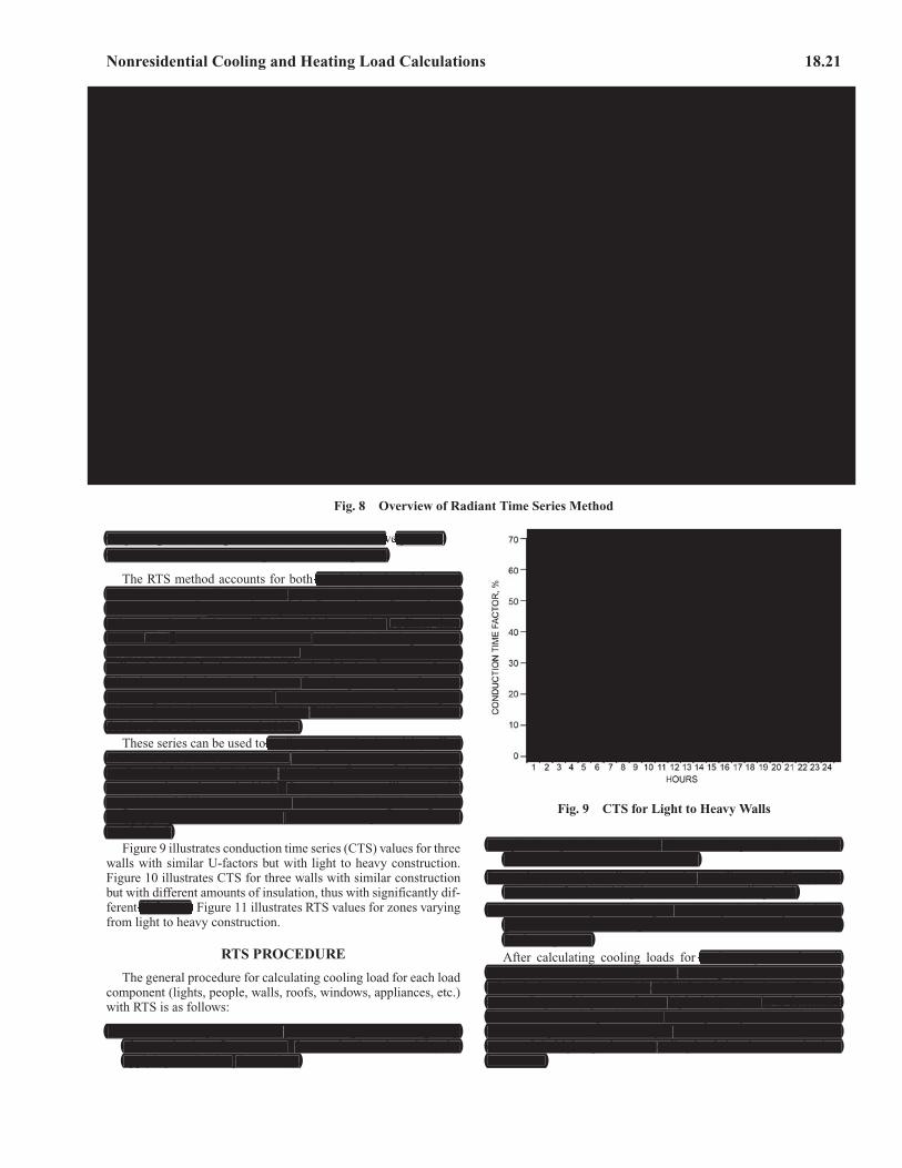
Nonresidential Cooling and Heating Load Calculations 18.21
• Splitting of all heat gains into radiant and convective portions• Conversion of radiant heat gains into cooling loads
The RTS method accounts for both conduction time delay andradiant time delay effects by multiplying hourly heat gains by 24 htime series. The time series multiplication, in effect, distributes heatgains over time. Series coefficients, which are called radiant timefactors and conduction time factors, are derived using the HBmethod. Radiant time factors reflect the percentage of an earlierradiant heat gain that becomes cooling load during the current hour.Likewise, conduction time factors reflect the percentage of an ear-lier heat gain at the exterior of a wall or roof that becomes heat gainindoors during the current hour. By definition, each radiant or con-duction time series must total 100%.
These series can be used to easily compare the time-delay effectof one construction versus another. This ability to compare choicesis of particular benefit during design, when all construction detailsmay not have been decided. Comparison can illustrate themagnitude of difference between the choices, allowing the engineerto apply judgment and make more informed assumptions in estimat-ing the load.
Figure 9 illustrates conduction time series (CTS) values for threewalls with similar U-factors but with light to heavy construction.Figure 10 illustrates CTS for three walls with similar constructionbut with different amounts of insulation, thus with significantly dif-ferent U-factors. Figure 11 illustrates RTS values for zones varyingfrom light to heavy construction.
RTS PROCEDURE
The general procedure for calculating cooling load for each loadcomponent (lights, people, walls, roofs, windows, appliances, etc.)with RTS is as follows:
1. Calculate 24 h profile of component heat gains for design day(for conduction, first account for conduction time delay byapplying conduction time series).
2. Split heat gains into radiant and convective parts (see Table 14for radiant and convective fractions).
3. Apply appropriate radiant time series to radiant part of heat gainsto account for time delay in conversion to cooling load.
4. Sum convective part of heat gain and delayed radiant part of heatgain to determine cooling load for each hour for each coolingload component.After calculating cooling loads for each component for each
hour, sum those to determine the total cooling load for each hour andselect the hour with the peak load for design of the air-conditioningsystem. Repeat this process for multiple design months to determinethe month when the peak load occurs, especially with windows onsouthern exposures (northern exposure in southern latitudes), whichcan result in higher peak room cooling loads in winter months thanin summer.
Fig. 8 Overview of Radiant Time Series Method
Fig. 9 CTS for Light to Heavy Walls
e portions• Conversion of radiant heat gains into cooling loads• Splitting of all heat gains into radiant and convectiv
conduction time delay andradiant time delay effects by multiplying hourly heat gains by 24 htime series. The time series multiplication, in effect, distributes heatgains over time. Series coefficients, which are called radiant timefactors and conduction time factors, are derived using the HBmethod. Radiant time factors reflect the percentage of an earlierradiant heat gain that becomes cooling load during the current hour.Likewise, conduction time factors reflect the percentage of an ear-lier heat gain at the exterior of a wall or roof that becomes heat gainindoors during the current hour. By definition, each radiant or con-duction time series must total 100%.
easily compare the time-delay effectof one construction versus another. This ability to compare choicesis of particular benefit during design, when all construction detailsmay not have been decided. Comparison can illustrate themagnitude of difference between the choices, allowing the engineerto apply judgment and make more informed assumptions in estimat-ing the load.
t U-factors.
1. Calculate 24 h profile of component heat gains for design daymm(for conduction, first account for conduction time delay byapplying conduction time series).
2. Split heat gains into radiant and convective parts (see Table 14for radiant and convective fractions).
3. Apply appropriate radiant time series to radiant part of heat gainsto account for time delay in conversion to cooling load.
4. Sum convective part of heat gain and delayed radiant part of heatgain to determine cooling load for each hour for each coolingload component.
each component for eachhour, sum those to determine the total cooling load for each hour andselect the hour with the peak load for design of the air-conditioningsystem. Repeat this process for multiple design months to determinethe month when the peak load occurs, especially with windows onsouthern exposures (northern exposure in southern latitudes), whichcan result in higher peak room cooling loads in winter months thanin summer.
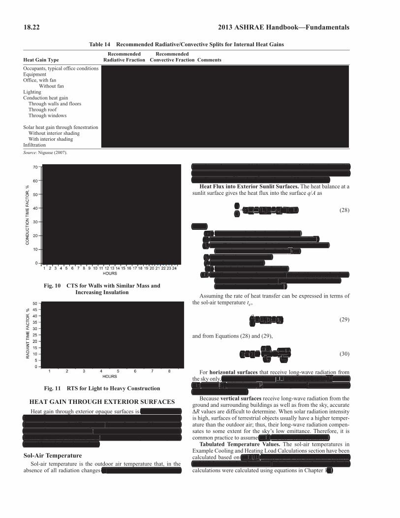
18.22 2013 ASHRAE Handbook—Fundamentals
HEAT GAIN THROUGH EXTERIOR SURFACES
Heat gain through exterior opaque surfaces is derived from thesame elements of solar radiation and thermal gradient as that forfenestration areas. It differs primarily as a function of the mass andnature of the wall or roof construction, because those elementsaffect the rate of conductive heat transfer through the compositeassembly to the interior surface.
Sol-Air TemperatureSol-air temperature is the outdoor air temperature that, in the
absence of all radiation changes gives the same rate of heat entry
into the surface as would the combination of incident solar radia-tion, radiant energy exchange with the sky and other outdoor sur-roundings, and convective heat exchange with outdoor air.
Heat Flux into Exterior Sunlit Surfaces. The heat balance at asunlit surface gives the heat flux into the surface q/A as
= �Et + ho(to – ts) – �R (28)
where� = absorptance of surface for solar radiationEt = total solar radiation incident on surface, Btu/h·ft2
ho = coefficient of heat transfer by long-wave radiation and convection at outer surface, Btu/h·ft2·°F
to = outdoor air temperature, °Fts = surface temperature, °F��= hemispherical emittance of surface
R = difference between long-wave radiation incident on surface from sky and surroundings and radiation emitted by blackbody at outdoor air temperature, Btu/h·ft2
Assuming the rate of heat transfer can be expressed in terms ofthe sol-air temperature te,
= ho(te – ts) (29)
and from Equations (28) and (29),
te = to + (30)
For horizontal surfaces that receive long-wave radiation fromthe sky only, an appropriate value of R is about 20 Btu/h·ft2, so thatif � = 1 and ho = 3.0 Btu/h·ft2·°F, the long-wave correction term isabout 7°F (Bliss 1961).
Because vertical surfaces receive long-wave radiation from theground and surrounding buildings as well as from the sky, accurateR values are difficult to determine. When solar radiation intensityis high, surfaces of terrestrial objects usually have a higher temper-ature than the outdoor air; thus, their long-wave radiation compen-sates to some extent for the sky’s low emittance. Therefore, it iscommon practice to assume �R = 0 for vertical surfaces.
Tabulated Temperature Values. The sol-air temperatures inExample Cooling and Heating Load Calculations section have beencalculated based on �R/ho values of 7°F for horizontal surfacesand 0°F for vertical surfaces; total solar intensity values used for thecalculations were calculated using equations in Chapter 14.
Table 14 Recommended Radiative/Convective Splits for Internal Heat Gains
Heat Gain TypeRecommended
Radiative FractionRecommended
Convective Fraction Comments
Occupants, typical office conditions 0.60 0.40 See Table 1 for other conditions.Equipment 0.1 to 0.8 0.9 to 0.2 See Tables 6 to 12 for details of equipment heat gain and recommended
radiative/convective splits for motors, cooking appliances, laboratory equipment, medical equipment, office equipment, etc.
Office, with fan 0.10 0.90Without fan 0.30 0.70
Lighting Varies; see Table 3.Conduction heat gain
Through walls and floors 0.46 0.54Through roof 0.60 0.40Through windows 0.33 (SHGC > 0.5)
0.46 (SHGC < 0.5)0.67 (SHGC > 0.5)0.54 (SHGC < 0.5)
Solar heat gain through fenestrationWithout interior shading 1.00 0.00With interior shading Varies; see Tables 13A to 13G in Chapter 15.
Infiltration 0.00 1.00
Source: Nigusse (2007).
Fig. 10 CTS for Walls with Similar Mass and Increasing Insulation
Fig. 11 RTS for Light to Heavy Construction
qA---
qA---
�Et
ho---------- � R
ho------------–
derived from thesame elements of solar radiation and thermal gradient as that forfenestration areas. It differs primarily as a function of the mass andnature of the wall or roof construction, because those elementsaffect the rate of conductive heat transfer through the compositeassembly to the interior surface.
gives the same rate of heat entry
into the surface as would the combination of incident solar radia-tion, radiant energy exchange with the sky and other outdoor sur-roundings, and convective heat exchange with outdoor air.
= ��E�� t t + ho(to – tst ) – ��Rq---A---
where� = absorptance of surface for solar radiation
ft2Et = total solar radiation incident on surface, Btu/h·fho = coefficient of heat transfer by long-wave radiation and
ft2convection at outer surface, Btu/h·f 2·°Fto = outdoor air temperature, °Ftst = surface temperature, °F� = hemispherical emittance of surface
R = difference between long-wave radiation incident on surface from sky and surroundings and radiation emitted by blackbody at
ft2outdoor air temperature, Btu/h·f
q---A--- = ho(tet – tst )
tet = tot + � Rt
ho
���Et�Et � Rho
ft2, , an appropriate value of R is about 20 Btu/h·f , so thatft2if � = 1 and ho = 3.0 Btu/h·f 2·°F, the long-wave correction term iso
about 7°F (Bliss 1961).
�R = 0 for vertical surfaces.
�R//ho values of 7°F for horizontal surfacesoand 0°F for vertical surfaces; total solar intensity values used for the
14.
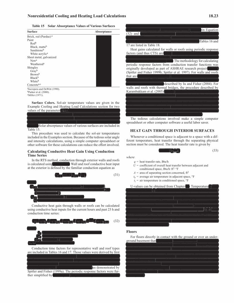
Nonresidential Cooling and Heating Load Calculations 18.23
Surface Colors. Sol-air temperature values are given in theExample Cooling and Heating Load Calculations section for twovalues of the parameter �/ho; the value of 0.15 is appropriate for alight-colored surface, whereas 0.30 represents the usual maximumvalue for this parameter (i.e., for a dark-colored surface or anysurface for which the permanent lightness cannot reliably be antic-ipated). Solar absorptance values of various surfaces are included inTable 15.
This procedure was used to calculate the sol-air temperaturesincluded in the Examples section. Because of the tedious solar angleand intensity calculations, using a simple computer spreadsheet orother software for these calculations can reduce the effort involved.
Calculating Conductive Heat Gain Using Conduction Time Series
In the RTS method, conduction through exterior walls and roofsis calculated using CTS values. Wall and roof conductive heat inputat the exterior is defined by the familiar conduction equation as
qi,�-n = UA(te,�-n – trc) (31)
whereqi,��n = conductive heat input for surface n hours ago, Btu/h
U = overall heat transfer coefficient for surface, Btu/h·ft2·°FA = surface area, ft2
te,�-n = sol-air temperature n hours ago, °Ftrc = presumed constant room air temperature, °F
Conductive heat gain through walls or roofs can be calculatedusing conductive heat inputs for the current hours and past 23 h andconduction time series:
q� = c0qi,� + c1qi,�-1 + c2qi,�-2 + c3qi,�-3 + … + c23qi,�-23 (32)
whereq� = hourly conductive heat gain for surface, Btu/h
qi,� = heat input for current hourqi,�-n = heat input n hours ago
c0, c1, etc. = conduction time factors
Conduction time factors for representative wall and roof typesare included in Tables 16 and 17. Those values were derived by firstcalculating conduction transfer functions for each example wall androof construction. Assuming steady-periodic heat input conditionsfor design load calculations allows conduction transfer functions tobe reformulated into periodic response factors, as demonstrated bySpitler and Fisher (1999a). The periodic response factors were fur-ther simplified by dividing the 24 periodic response factors by the
respective overall wall or roof U-factor to form the conduction timeseries. The conduction time factors can then be used in Equation(32) and provide a way to compare time delay characteristicsbetween different wall and roof constructions. Construction mate-rial data used in the calculations for walls and roofs in Tables 16 and17 are listed in Table 18.
Heat gains calculated for walls or roofs using periodic responsefactors (and thus CTS) are identical to those calculated using con-duction transfer functions for the steady periodic conditions assumedin design cooling load calculations. The methodology for calculatingperiodic response factors from conduction transfer functions wasoriginally developed as part of ASHRAE research project RP-875(Spitler and Fisher 1999b; Spitler et al. 1997). For walls and roofsthat are not reasonably close to the representative constructions inTables 16 and 17, CTS coefficients may be computed with a com-puter program such as that described by Iu and Fisher (2004). Forwalls and roofs with thermal bridges, the procedure described byKarambakkam et al. (2005) may be used to determine an equivalentwall construction, which can then be used as the basis for finding theCTS coefficients. When considering the level of detail needed tomake an adequate approximation, remember that, for buildings withwindows and internal heat gains, the conduction heat gains make upa relatively small part of the cooling load. For heating load calcula-tions, the conduction heat loss may be more significant.
The tedious calculations involved make a simple computerspreadsheet or other computer software a useful labor saver.
HEAT GAIN THROUGH INTERIOR SURFACES
Whenever a conditioned space is adjacent to a space with a dif-ferent temperature, heat transfer through the separating physicalsection must be considered. The heat transfer rate is given by
q = UA(tb – ti) (33)
whereq = heat transfer rate, Btu/hU = coefficient of overall heat transfer between adjacent and
conditioned space, Btu/h·ft2·°FA = area of separating section concerned, ft2
tb = average air temperature in adjacent space, °Fti = air temperature in conditioned space, °F
U-values can be obtained from Chapter 27. Temperature tb maydiffer greatly from ti. The temperature in a kitchen or boiler room,for example, may be as much as 15 to 50°F above the outdoor airtemperature. Actual temperatures in adjoining spaces should bemeasured, when possible. Where nothing is known except that theadjacent space is of conventional construction, contains no heatsources, and itself receives no significant solar heat gain, tb – ti maybe considered the difference between the outdoor air and condi-tioned space design dry-bulb temperatures minus 5°F. In somecases, air temperature in the adjacent space corresponds to the out-door air temperature or higher.
FloorsFor floors directly in contact with the ground or over an under-
ground basement that is neither ventilated nor conditioned, sensibleheat transfer may be neglected for cooling load estimates becauseusually there is a heat loss rather than a gain. An exception is in hotclimates (i.e., where average outdoor air temperature exceedsindoor design condition), where the positive soil-to-indoor temper-ature difference causes sensible heat gains (Rock 2005). In manyclimates and for various temperatures and local soil conditions,moisture transport up through slabs-on-grade and basement floors isalso significant, and contributes to the latent heat portion of thecooling load.
Table 15 Solar Absorptance Values of Various Surfaces
Surface Absorptance
Brick, red (Purdue) a 0.63Paint
Redb 0.63Black, matteb 0.94Sandstoneb 0.50White acrylica 0.26
Sheet metal, galvanizedNewa 0.65Weathereda 0.80
Shingles 0.82Grayb
Brownb 0.91Blackb 0.97Whiteb 0.75
Concretea,c 0.60 to 0.83aIncropera and DeWitt (1990).bParker et al. (2000).cMiller (1971).
�//ho; the value of 0.15 is appropriate for aolight-colored surface, whereas 0.30 represents the usual maximumvalue for this parameter (i.e., for a dark-colored surface or anysurface for which the permanent lightness cannot reliably be antic-ipated).
g CTS values.
qi, = UA((te, – trct ),�--n ,�--n
whereqi, = conductive heat input for surface n hours ago, Btu/h,��n
ft2U = overall heat transfer coefficient for surface, Btu/h·fU 2·°Fft2A = surface area,
te, = sol-air temperature n hours ago, °F,�--n trct = presumed constant room air temperature, °F
… q = c0qi, + c1qi, + c2qi, + c3qi, + + c23qi,q� ,� ,�--1 ,�--2 ,�--3 ,�--23
whereq = hourly conductive heat gain for surface, Btu/hq�
qi, = heat input for current hour,� qi, = heat input n hours ago,��-n
c0, c1, i,� netc. = conduction time factors
calculating conduction transfer functions for each example wall androof construction. Assuming steady-periodic heat input conditionsfor design load calculations allows conduction transfer functions tobe reformulated into periodic response factors,
dividing the 24 periodic response factors by the
respective overall wall or roof U-factor to form the conduction timeseries. The conduction time factors can then be used
provide a way to compare time delay characteristicsbetween different wall and roof constructions. Construction mate-rial data used in the calculations for walls and roofs in T
identical to those calculated using con-duction transfer functions for the steady periodic conditions assumedin design cooling load calculations.
RP-875
not reasonably close to the representative constructions inTables 16 and 17, CTS coefficients may be computed with a com-puter program such as that
may be used to determine an equivalentwall construction, which can then be used as the basis for finding theCTS coefficients. When considering the level of detail needed tomake an adequate approximation, remember that, for buildings withwindows and internal heat gains, the conduction heat gains make upa relatively small part of the cooling load. For heating load calcula-tions, the conduction heat loss may be more significant.
q = UA((tb – – ti)
27. tb maydiffer greatly from ti.
bThe temperature in a kitchen or boiler room,i
for example, may be as much as 15 to 50°F above the outdoor airtemperature. Actual temperatures in adjoining spaces should bemeasured, when possible. Where nothing is known except that thettadjacent space is of conventional construction, contains no heatsources, and itself receives no significant solar heat gain, tb – – ti mayb ibe considered the difference between the outdoor air and condi-tioned space design dry-bulb temperatures minus 5°F. In somecases, air temperature in the adjacent space corresponds to the out-door air temperature or higher.
t is neither ventilated nor conditioned, sensibleheat transfer may be neglected for cooling load estimates becauseusually there is a heat loss rather than a gain. An exception is in hotclimates (i.e., where average outdoor air temperature exceedsindoor design condition), where the positive soil-to-indoor temper-ature difference causes sensible heat gains (Rock 2005). In manyclimates and for various temperatures and local soil conditions,moisture transport up through slabs-on-grade and basement floors isalso significant, and contributes to the latent heat portion of thecooling load.
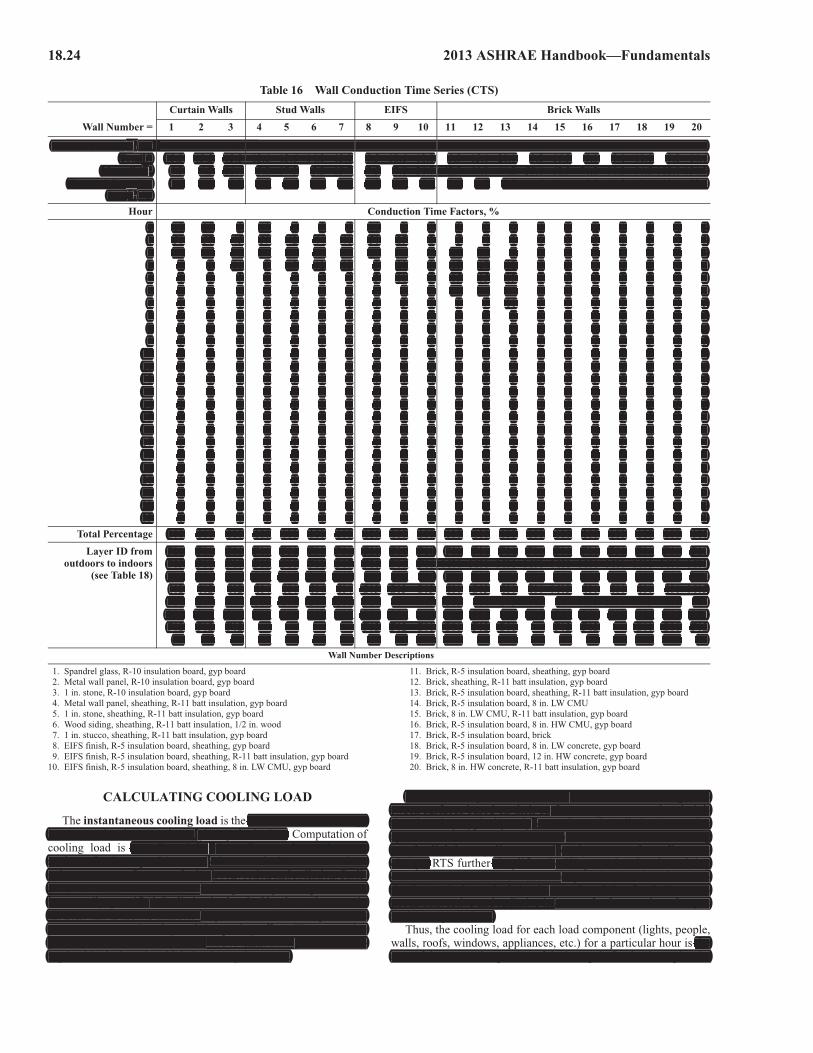
18.24 2013 ASHRAE Handbook—Fundamentals
CALCULATING COOLING LOAD
The instantaneous cooling load is the rate at which heat energyis convected to the zone air at a given point in time. Computation ofcooling load is complicated by the radiant exchange betweensurfaces, furniture, partitions, and other mass in the zone. Most heatgain sources transfer energy by both convection and radiation. Radi-ative heat transfer introduces a time dependency to the process thatis not easily quantified. Radiation is absorbed by thermal masses inthe zone and then later transferred by convection into the space. Thisprocess creates a time lag and dampening effect. The convectiveportion, on the other hand, is assumed to immediately become cool-ing load in the hour in which that heat gain occurs.
Heat balance procedures calculate the radiant exchange be-tween surfaces based on their surface temperatures and emissivi-ties, but they typically rely on estimated “radiative/convectivesplits” to determine the contribution of internal loads, includingpeople, lighting, appliances, and equipment, to the radiant ex-change. RTS further simplifies the HB procedure by also relyingon an estimated radiative/convective split of wall and roof conduc-tive heat gain instead of simultaneously solving for the instanta-neous convective and radiative heat transfer from each surface, asin the HB procedure.
Thus, the cooling load for each load component (lights, people,walls, roofs, windows, appliances, etc.) for a particular hour is thesum of the convective portion of the heat gain for that hour plus the
Table 16 Wall Conduction Time Series (CTS)
Wall Number =
Curtain Walls Stud Walls EIFS Brick Walls
1 2 3 4 5 6 7 8 9 10 11 12 13 14 15 16 17 18 19 20
U-Factor, Btu/h·ft2·°F 0.075 0.076 0.075 0.074 0.074 0.071 0.073 0.118 0.054 0.092 0.101 0.066 0.050 0.102 0.061 0.111 0.124 0.091 0.102 0.068Total R 13.3 13.2 13.3 13.6 13.6 14.0 13.8 8.5 18.6 10.8 9.9 15.1 20.1 9.8 16.3 9.0 8.1 11.0 9.8 14.6
Mass, lb/ft2 6.3 4.3 16.4 5.2 17.3 5.2 13.7 7.5 7.8 26.8 42.9 44.0 44.2 59.6 62.3 76.2 80.2 96.2 182.8 136.3Thermal Capacity,
Btu/ft2·°F1.5 1.0 3.3 1.2 3.6 1.6 3.0 1.8 1.9 5.9 8.7 8.7 8.7 11.7 12.4 15.7 15.3 19.0 38.4 28.4
Hour Conduction Time Factors, %
0 18 25 8 19 6 7 5 11 2 1 0 0 0 1 2 2 1 3 4 31 58 57 45 59 42 44 41 50 25 2 5 4 1 1 2 2 1 3 4 32 20 15 32 18 33 32 34 26 31 6 14 13 7 2 2 2 3 3 4 33 4 3 11 3 13 12 13 9 20 9 17 17 12 5 3 4 6 3 4 44 0 0 3 1 4 4 4 3 11 9 15 15 13 8 5 5 7 3 4 45 0 0 1 0 1 1 2 1 5 9 12 12 13 9 6 6 8 4 4 46 0 0 0 0 1 0 1 0 3 8 9 9 11 9 7 6 8 4 4 57 0 0 0 0 0 0 0 0 2 7 7 7 9 9 7 7 8 5 4 58 0 0 0 0 0 0 0 0 1 6 5 5 7 8 7 7 8 5 4 59 0 0 0 0 0 0 0 0 0 6 4 4 6 7 7 6 7 5 4 5
10 0 0 0 0 0 0 0 0 0 5 3 3 5 7 6 6 6 5 4 511 0 0 0 0 0 0 0 0 0 5 2 2 4 6 6 6 6 5 5 512 0 0 0 0 0 0 0 0 0 4 2 2 3 5 5 5 5 5 5 513 0 0 0 0 0 0 0 0 0 4 1 2 2 4 5 5 4 5 5 514 0 0 0 0 0 0 0 0 0 3 1 2 2 4 5 5 4 5 5 515 0 0 0 0 0 0 0 0 0 3 1 1 1 3 4 4 3 5 4 416 0 0 0 0 0 0 0 0 0 3 1 1 1 3 4 4 3 5 4 417 0 0 0 0 0 0 0 0 0 2 1 1 1 2 3 4 3 4 4 418 0 0 0 0 0 0 0 0 0 2 0 0 1 2 3 3 2 4 4 419 0 0 0 0 0 0 0 0 0 2 0 0 1 2 3 3 2 4 4 420 0 0 0 0 0 0 0 0 0 2 0 0 0 1 3 3 2 4 4 421 0 0 0 0 0 0 0 0 0 1 0 0 0 1 2 2 1 4 4 422 0 0 0 0 0 0 0 0 0 1 0 0 0 1 2 2 1 4 4 323 0 0 0 0 0 0 0 0 0 0 0 0 0 0 1 1 1 3 4 3
Total Percentage 100 100 100 100 100 100 100 100 100 100 100 100 100 100 100 100 100 100 100 100
Layer ID fromoutdoors to indoors
(see Table 18)
F01 F01 F01 F01 F01 F01 F01 F01 F01 F01 F01 F01 F01 F01 F01 F01 F01 F01 F01 F01F09 F08 F10 F08 F10 F11 F07 F06 F06 F06 M01 M01 M01 M01 M01 M01 M01 M01 M01 M01F04 F04 F04 G03 G03 G02 G03 I01 I01 I01 F04 F04 F04 F04 F04 F04 F04 F04 F04 F04I02 I02 I02 I04 I04 I04 I04 G03 G03 G03 I01 G03 I01 I01 M03 I01 I01 I01 I01 M15F04 F04 F04 G01 G01 G04 G01 F04 I04 M03 G03 I04 G03 M03 I04 M05 M01 M13 M16 I04G01 G01 G01 F02 F02 F02 F02 G01 G01 F04 F04 G01 I04 F02 G01 G01 F02 F04 F04 G01F02 F02 F02 — — — — F02 F02 G01 G01 F02 G01 — F02 F02 — G01 G01 F02
— — — — — — — — — F02 F02 — F02 — — — — F02 F02 —
Wall Number Descriptions
1. Spandrel glass, R-10 insulation board, gyp board2. Metal wall panel, R-10 insulation board, gyp board3. 1 in. stone, R-10 insulation board, gyp board4. Metal wall panel, sheathing, R-11 batt insulation, gyp board5. 1 in. stone, sheathing, R-11 batt insulation, gyp board6. Wood siding, sheathing, R-11 batt insulation, 1/2 in. wood7. 1 in. stucco, sheathing, R-11 batt insulation, gyp board8. EIFS finish, R-5 insulation board, sheathing, gyp board9. EIFS finish, R-5 insulation board, sheathing, R-11 batt insulation, gyp board
10. EIFS finish, R-5 insulation board, sheathing, 8 in. LW CMU, gyp board
11. Brick, R-5 insulation board, sheathing, gyp board12. Brick, sheathing, R-11 batt insulation, gyp board13. Brick, R-5 insulation board, sheathing, R-11 batt insulation, gyp board14. Brick, R-5 insulation board, 8 in. LW CMU15. Brick, 8 in. LW CMU, R-11 batt insulation, gyp board16. Brick, R-5 insulation board, 8 in. HW CMU, gyp board17. Brick, R-5 insulation board, brick18. Brick, R-5 insulation board, 8 in. LW concrete, gyp board19. Brick, R-5 insulation board, 12 in. HW concrete, gyp board20. Brick, 8 in. HW concrete, R-11 batt insulation, gyp board
ft2U-Factor, Btu/h·f 0.101 0.066 0.050 0.102 0.061 0.111 0.124 0.091 0.102 0.0680.118 0.054 0.0920.074 0.074 0.071 0.0732·°F 0.075 0.076 0.075Total R 13.3 13.2 13.6 13.6 14.0 13.813.3 8.5 18.6 10.8 9.9 15.1 20.1 9.8 16.3 9.0 8.1 11.0 9.8 14.6
ft2Mass, lb/f 6.3 4.3 16.4 5.2 17.3 5.2 13.7 7.5 42.9 44.0 44.2 59.6 62.3 76.2 80.2 96.2 182.8 136.37.8 26.8Thermal Capacity, 1.5 1.0 3.3 1.2 3.6 1.6 3.0 1.8 1.9 5.9 8.7 8.7 8.7 11.7 12.4 15.7 15.3 19.0 38.4 28.4p
ft2Btu/f 2·°F
0 18 25 8 19 6 7 5 11 2 1 0 0 0 1 2 2 1 3 4 31 58 57 45 59 42 44 41 50 25 2 5 4 1 1 2 2 1 3 4 32 20 15 32 18 33 32 34 26 31 6 14 13 7 2 2 2 3 3 4 33 4 3 11 3 13 12 13 9 20 9 17 17 12 5 3 4 6 3 4 44 0 0 3 1 4 4 4 3 11 9 15 15 13 8 5 5 7 3 4 45 0 0 1 0 1 1 2 1 5 9 12 12 13 9 6 6 8 4 4 46 0 0 0 0 1 0 1 0 3 8 9 9 11 9 7 6 8 4 4 57 0 0 0 0 0 0 0 0 2 7 7 7 9 9 7 7 8 5 4 58 0 0 0 0 0 0 0 0 1 6 5 5 7 8 7 7 8 5 4 59 0 0 0 0 0 0 0 0 0 6 4 4 6 7 7 6 7 5 4 5
10 0 0 0 0 0 0 0 0 0 5 3 3 5 7 6 6 6 5 4 511 0 0 0 0 0 0 0 0 0 5 2 2 4 6 6 6 6 5 5 512 0 0 0 0 0 0 0 0 0 4 2 2 3 5 5 5 5 5 5 513 0 0 0 0 0 0 0 0 0 4 1 2 2 4 5 5 4 5 5 514 0 0 0 0 0 0 0 0 0 3 1 2 2 4 5 5 4 5 5 515 0 0 0 0 0 0 0 0 0 3 1 1 1 3 4 4 3 5 4 416 0 0 0 0 0 0 0 0 0 3 1 1 1 3 4 4 3 5 4 417 0 0 0 0 0 0 0 0 0 2 1 1 1 2 3 4 3 4 4 418 0 0 0 0 0 0 0 0 0 2 0 0 1 2 3 3 2 4 4 419 0 0 0 0 0 0 0 0 0 2 0 0 1 2 3 3 2 4 4 420 0 0 0 0 0 0 0 0 0 2 0 0 0 1 3 3 2 4 4 421 0 0 0 0 0 0 0 0 0 1 0 0 0 1 2 2 1 4 4 422 0 0 0 0 0 0 0 0 0 1 0 0 0 1 2 2 1 4 4 323 0 0 0 0 0 0 0 0 0 0 0 0 0 0 1 1 1 3 4 3
100 100 100 100 100 100 100 100 100 100 100 100 100 100 100 100 100 100 100 100
F01 F01 F01 F01 F01 F01 F01 F01 F01 F01 F01 F01 F01 F01 F01 F01 F01 F01 F01 F01F09 F08 F10 F08 F10 F11 F07 F06 F06 F06 M01 M01 M01 M01 M01 M01 M01 M01 M01 M01F04 F04 F04 G03 G03 G02 G03 I01 I01 I01 F04 F04 F04 F04 F04 F04 F04 F04 F04 F04I02 I02 I02 I04 I04 I04 I04 G03 G03 G03 I01 G03 I01 I01 M03 I01 I01 I01 I01 M15F04 F04 F04 G01 G01 G04 G01 F04 I04 M03 G03 I04 G03 M03 I04 M05 M01 M13 M16 I04G01 G01 G01 F02 F02 F02 F02 G01 G01 F04 F04 G01 I04 F02 G01 G01 F02 F04 F04 G01F02 F02 F02 — — — — F02 F02 G01 G01 F02 G01 — F02 F02 — G01 G01 F02
— — — — — — — — — F02 F02 — F02 — — — — F02 F02 —
rate at which heat energyis convected to the zone air at a given point in time.
complicated by the radiant exchange betweensurfaces, furniture, partitions, and other mass in the zone. Most heatgain sources transfer energy by both convection and radiation. Radi-ative heat transfer introduces a time dependency to the process thatis not easily quantified. Radiation is absorbed by thermal masses inthe zone and then later transferred by convection into the space. Thisprocess creates a time lag and dampening effect. The convectiveportion, on the other hand, is assumed to immediateluu y become cool-ing load in the hour in which that heat gain occurs.
Heat balance procedures calculate the radiant exchange be-tween surfaces based on their surface temperatures and emissivi-ties, but they typically rely on estimated “radiative/convectivesplits” to determine the contribution of internal loads, includingpeople, lighting, appliances, and equipment, to the radiant ex-change. simplifies the HB procedure by also relyingon an estimated radiative/convective split of wall and roof conduc-tive heat gain instead of simultaneously solving for the instanta-neous convective and radiative heat transfer from each surface, asin the HB procedure.
thesum of the convective portion of the heat gain for that hour plus the
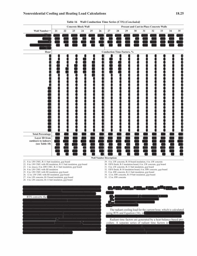
Nonresidential Cooling and Heating Load Calculations 18.25
time-delayed portion of radiant heat gains for that hour and the pre-vious 23 h. Table 14 contains recommendations for splitting each ofthe heat gain components into convective and radiant portions.
RTS converts the radiant portion of hourly heat gains to hourlycooling loads using radiant time factors, the coefficients of the radi-ant time series. Radiant time factors are used to calculate the coolingload for the current hour on the basis of current and past heat gains.The radiant time series for a particular zone gives the time-dependent response of the zone to a single pulse of radiant energy.The series shows the portion of the radiant pulse that is convected tozone air for each hour. Thus, r0 represents the fraction of the radiantpulse convected to the zone air in the current hour r1 in the previoushour, and so on. The radiant time series thus generated is used toconvert the radiant portion of hourly heat gains to hourly coolingloads according to the following equation:
Qr,� = r0qr,� + r1qr,� –1 + r2qr,� –2 + r3qr,� –3 + … + r23qr,� –23 (34)
whereQr, � = radiant cooling load Qr for current hour �, Btu/hqr, � = radiant heat gain for current hour, Btu/h
qr,��n = radiant heat gain n hours ago, Btu/hr0, r1, etc.=radiant time factors
The radiant cooling load for the current hour, which is calculatedusing RTS and Equation (34), is added to the convective portion todetermine the total cooling load for that component for that hour.
Radiant time factors are generated by a heat-balance-based pro-cedure. A separate series of radiant time factors is theoreticallyrequired for each unique zone and for each unique radiant energydistribution function assumption. For most common design applica-tions, RTS variation depends primarily on the overall massiveness
Table 16 Wall Conduction Time Series (CTS) (Concluded)
Wall Number =
Concrete Block Wall Precast and Cast-in-Place Concrete Walls
21 22 23 24 25 26 27 28 29 30 31 32 33 34 35
U-Factor, Btu/h·ft2·°F 0.067 0.059 0.073 0.186 0.147 0.121 0.118 0.074 0.076 0.115 0.068 0.082 0.076 0.047 0.550Total R 14.8 16.9 13.7 5.4 6.8 8.2 8.4 13.6 13.1 8.7 14.7 12.2 13.1 21.4 1.8
Mass, lb/ft2 22.3 22.3 46.0 19.3 21.9 34.6 29.5 29.6 53.8 59.8 56.3 100.0 96.3 143.2 140.0Thermal Capacity,
Btu/ft2·°F4.8 4.8 10.0 4.1 4.7 7.4 6.1 6.1 10.8 12.1 11.4 21.6 20.8 30.9 30.1
Hour Conduction Time Factors, %
0 0 1 0 1 0 1 1 0 1 2 1 3 1 2 11 4 1 2 11 3 1 10 8 1 2 2 3 2 2 22 13 5 8 21 12 2 20 18 3 3 3 4 5 3 43 16 9 12 20 16 5 18 18 6 5 6 5 8 3 74 14 11 12 15 15 7 14 14 8 6 7 6 9 5 85 11 10 11 10 12 9 10 11 9 6 8 6 9 5 86 9 9 9 7 10 9 7 8 9 6 8 6 8 6 87 7 8 8 5 8 8 5 6 9 6 7 5 7 6 88 6 7 7 3 6 8 4 4 8 6 7 5 6 6 79 4 6 6 2 4 7 3 3 7 6 6 5 6 6 6
10 3 5 5 2 3 6 2 2 7 5 6 5 5 6 611 3 4 4 1 3 6 2 2 6 5 5 5 5 5 512 2 4 3 1 2 5 1 2 5 5 5 4 4 5 413 2 3 2 1 2 4 1 1 4 5 4 4 4 5 414 2 3 2 0 1 4 1 1 4 4 4 4 3 4 415 1 3 2 0 1 3 1 1 3 4 3 4 3 4 316 1 2 1 0 1 3 0 1 2 4 3 4 3 4 317 1 2 1 0 1 2 0 0 2 3 3 4 2 4 318 1 2 1 0 0 2 0 0 1 3 2 4 2 4 219 0 1 1 0 0 2 0 0 1 3 2 3 2 3 220 0 1 1 0 0 2 0 0 1 3 2 3 2 3 221 0 1 1 0 0 2 0 0 1 3 2 3 2 3 122 0 1 1 0 0 1 0 0 1 3 2 3 1 3 123 0 1 0 0 0 1 0 0 1 2 2 2 1 3 1
Total Percentage 100 100 100 100 100 100 100 100 100 100 100 100 100 100 100
Layer ID fromoutdoors to indoors
(see Table 18)
F01 F01 F01 F01 F01 F01 F01 F01 F01 F01 F01 F01 F01 F01 F01M03 M08 F07 M08 M08 M09 M11 M11 M11 F06 M13 F06 M15 M16 M16
I04 I04 M05 F02 F04 F04 I01 I04 I02 I01 I04 I02 I04 I05 F02G01 G01 I04 — G01 G01 F04 G01 M11 M13 G01 M15 G01 G01 —F02 F02 G01 — F02 F02 G01 F02 F02 G01 F02 G01 F02 F02 —
— — F02 — — — F02 — — F02 — F02 — — —
Wall Number Descriptions
21. 8 in. LW CMU, R-11 batt insulation, gyp board22. 8 in. LW CMU with fill insulation, R-11 batt insulation, gyp board23. 1 in. stucco, 8 in. HW CMU, R-11 batt insulation, gyp board24. 8 in. LW CMU with fill insulation25. 8 in. LW CMU with fill insulation, gyp board26. 12 in. LW CMU with fill insulation, gyp board27. 4 in. LW concrete, R-5 board insulation, gyp board28. 4 in. LW concrete, R-11 batt insulation, gyp board
29. 4 in. LW concrete, R-10 board insulation, 4 in. LW concrete30. EIFS finish, R-5 insulation board, 8 in. LW concrete, gyp board31. 8 in. LW concrete, R-11 batt insulation, gyp board32. EIFS finish, R-10 insulation board, 8 in. HW concrete, gyp board33. 8 in. HW concrete, R-11 batt insulation, gyp board34. 12 in. HW concrete, R-19 batt insulation, gyp board35. 12 in. HW concrete
ft2U-Factor, Btu/h·f 2·°F 0.067 0.059 0.073 0.186 0.147 0.121 0.118 0.074 0.076 0.115 0.068 0.082 0.076 0.047 0.550Total R 14.8 16.9 13.7 5.4 6.8 8.2 8.4 13.6 13.1 8.7 14.7 12.2 13.1 21.4 1.8
ft2Mass, lb/f 22.3 22.3 46.0 19.3 21.9 34.6 29.5 29.6 53.8 59.8 56.3 100.0 96.3 143.2 140.0Thermal Capacity, 4.8 4.8 10.0 4.1 4.7 7.4 6.1 6.1 10.8 12.1 11.4 21.6 20.8 30.9 30.1p
ft2Btu/f 2·°F
0 0 1 0 1 0 1 1 0 1 2 1 3 1 2 11 4 1 2 11 3 1 10 8 1 2 2 3 2 2 22 13 5 8 21 12 2 20 18 3 3 3 4 5 3 43 16 9 12 20 16 5 18 18 6 5 6 5 8 3 74 14 11 12 15 15 7 14 14 8 6 7 6 9 5 85 11 10 11 10 12 9 10 11 9 6 8 6 9 5 86 9 9 9 7 10 9 7 8 9 6 8 6 8 6 87 7 8 8 5 8 8 5 6 9 6 7 5 7 6 88 6 7 7 3 6 8 4 4 8 6 7 5 6 6 79 4 6 6 2 4 7 3 3 7 6 6 5 6 6 6
10 3 5 5 2 3 6 2 2 7 5 6 5 5 6 611 3 4 4 1 3 6 2 2 6 5 5 5 5 5 512 2 4 3 1 2 5 1 2 5 5 5 4 4 5 413 2 3 2 1 2 4 1 1 4 5 4 4 4 5 414 2 3 2 0 1 4 1 1 4 4 4 4 3 4 415 1 3 2 0 1 3 1 1 3 4 3 4 3 4 316 1 2 1 0 1 3 0 1 2 4 3 4 3 4 317 1 2 1 0 1 2 0 0 2 3 3 4 2 4 318 1 2 1 0 0 2 0 0 1 3 2 4 2 4 219 0 1 1 0 0 2 0 0 1 3 2 3 2 3 220 0 1 1 0 0 2 0 0 1 3 2 3 2 3 221 0 1 1 0 0 2 0 0 1 3 2 3 2 3 122 0 1 1 0 0 1 0 0 1 3 2 3 1 3 123 0 1 0 0 0 1 0 0 1 2 2 2 1 3 1
100 100 100 100 100 100 100 100 100 100 100 100 100 100 100
F01 F01 F01 F01 F01 F01 F01 F01 F01 F01 F01 F01 F01 F01 F01M03 M08 F07 M08 M08 M09 M11 M11 M11 F06 M13 F06 M15 M16 M16
I04 I04 M05 F02 F04 F04 I01 I04 I02 I01 I04 I02 I04 I05 F02G01 G01 I04 — G01 G01 F04 G01 M11 M13 G01 M15 G01 G01 —F02 F02 G01 — F02 F02 G01 F02 F02 G01 F02 G01 F02 F02 —
— — F02 — — — F02 — — F02 — F02 — — —
time-delayed portion of radiant heat gains for that hour and the pre-vious 23 h. Table 14 contains recommendations for splitting each ofthe heat gain components into convective and radiant portions.
radiant portion of hourly heat gains to hourlycooling loads using radiant time factors, the coefficients of the radi-ant time series. Radiant time factors are used to calculate the coolingload for the current hour on the basis of current and past heat gains.The radiant time series for a particular zone gives the time-dependent response of the zone to a single pulse of radiant energy.The series shows the portion of the radiant pulse that is convected tozone air for each hour. Thus, r0 represents the fraction of the radiant0pulse convected to the zone air in the current hour r r1 in the previous1hour, and so on. The radiant time series thus generated is used toconvert the radiant portion of hourly heat gains to hourly coolingloads according to the following equation:
… Qr, = r0qr, + r1qr, + r2qr, + r3qr, + + r23qr, (34)r,� r,� r,� ––1 r,� ––2 r,� ––3 r,� ––23
whereQr, = radiant cooling load Qr r for current hour �, Btu/h� ,qr, = radiant heat gain for current hour, Btu/h�
qr, = radiant heat gain n hours ago, Btu/h��n,r0, r1, etc.=radiant time factors
added to the convective portion todetermine the total cooling load for that component for that hour.
theoreticallyrequired for each unique zone and for each unique radiant energydistribution function assumption. For most common design applica-tions, RTS variation depends primarily on the overall massiveness
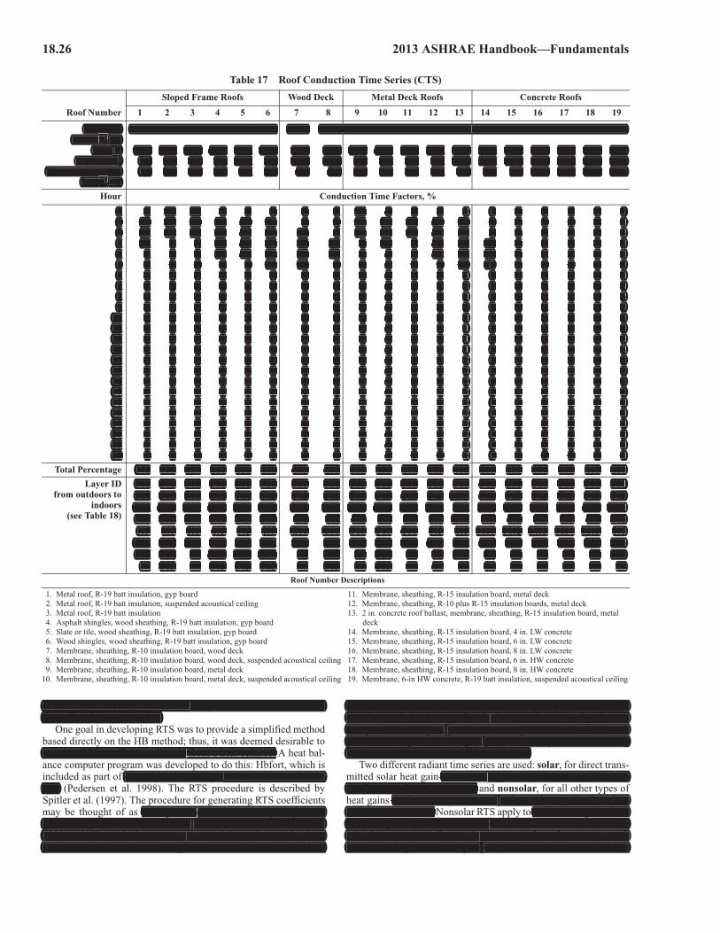
18.26 2013 ASHRAE Handbook—Fundamentals
of the construction and the thermal responsiveness of the surfacesthe radiant heat gains strike.
One goal in developing RTS was to provide a simplified methodbased directly on the HB method; thus, it was deemed desirable togenerate RTS coefficients directly from a heat balance. A heat bal-ance computer program was developed to do this: Hbfort, which isincluded as part of Cooling and Heating Load Calculation Princi-ples (Pedersen et al. 1998). The RTS procedure is described bySpitler et al. (1997). The procedure for generating RTS coefficientsmay be thought of as analogous to the custom weighting factorgeneration procedure used by DOE 2.1 (Kerrisk et al. 1981; Sowell1988a, 1988b). In both cases, a zone model is pulsed with a heatgain. With DOE 2.1, the resulting loads are used to estimate the best
values of the transfer function method weighting factors to mostclosely match the load profile. In the procedure described here, aunit periodic heat gain pulse is used to generate loads for a 24 hperiod. As long as the heat gain pulse is a unit pulse, the resultingloads are equivalent to the RTS coefficients.
Two different radiant time series are used: solar, for direct trans-mitted solar heat gain (radiant energy assumed to be distributed tothe floor and furnishings only) and nonsolar, for all other types ofheat gains (radiant energy assumed to be uniformly distributed onall internal surfaces). Nonsolar RTS apply to radiant heat gains frompeople, lights, appliances, walls, roofs, and floors. Also, for diffusesolar heat gain and direct solar heat gain from fenestration withindoor shading (blinds, drapes, etc.), the nonsolar RTS should be
Table 17 Roof Conduction Time Series (CTS)
Sloped Frame Roofs Wood Deck Metal Deck Roofs Concrete Roofs
Roof Number 1 2 3 4 5 6 7 8 9 10 11 12 13 14 15 16 17 18 19
U-Factor,Btu/h·ft2·°F
0.044 0.040 0.045 0.041 0.042 0.041 0.069 0.058 0.080 0.065 0.057 0.036 0.052 0.054 0.052 0.051 0.056 0.055 0.042
Total R 22.8 25.0 22.2 24.1 23.7 24.6 14.5 17.2 12.6 15.4 17.6 27.6 19.1 18.6 19.2 19.7 18.0 18.2 23.7Mass, lb/ft2 5.5 4.3 2.9 7.1 11.4 7.1 10.0 11.5 4.9 6.3 5.1 5.6 11.8 30.6 43.9 57.2 73.9 97.2 74.2
Thermal Capacity,Btu/ft2·°F
1.3 0.8 0.6 2.3 3.6 2.3 3.7 3.9 1.4 1.6 1.4 1.6 2.8 6.6 9.3 12.0 16.3 21.4 16.2
Hour Conduction Time Factors, %
0 6 10 27 1 1 1 0 1 18 4 8 1 0 1 2 2 2 3 11 45 57 62 17 17 12 7 3 61 41 53 23 10 2 2 2 2 3 22 33 27 10 31 34 25 18 8 18 35 30 38 22 8 3 3 5 3 63 11 5 1 24 25 22 18 10 3 14 7 22 20 11 6 4 6 5 84 3 1 0 14 13 15 15 10 0 4 2 10 14 11 7 5 7 6 85 1 0 0 7 6 10 11 9 0 1 0 4 10 10 8 6 7 6 86 1 0 0 4 3 6 8 8 0 1 0 2 7 9 8 6 6 6 77 0 0 0 2 1 4 6 7 0 0 0 0 5 7 7 6 6 6 78 0 0 0 0 0 2 5 6 0 0 0 0 4 6 7 6 6 6 69 0 0 0 0 0 1 3 5 0 0 0 0 3 5 6 6 5 5 5
10 0 0 0 0 0 1 3 5 0 0 0 0 2 5 5 6 5 5 511 0 0 0 0 0 1 2 4 0 0 0 0 1 4 5 5 5 5 512 0 0 0 0 0 0 1 4 0 0 0 0 1 3 5 5 4 5 413 0 0 0 0 0 0 1 3 0 0 0 0 1 3 4 5 4 4 414 0 0 0 0 0 0 1 3 0 0 0 0 0 3 4 4 4 4 315 0 0 0 0 0 0 1 3 0 0 0 0 0 2 3 4 4 4 316 0 0 0 0 0 0 0 2 0 0 0 0 0 2 3 4 3 4 317 0 0 0 0 0 0 0 2 0 0 0 0 0 2 3 4 3 4 318 0 0 0 0 0 0 0 2 0 0 0 0 0 1 3 3 3 3 219 0 0 0 0 0 0 0 2 0 0 0 0 0 1 2 3 3 3 220 0 0 0 0 0 0 0 1 0 0 0 0 0 1 2 3 3 3 221 0 0 0 0 0 0 0 1 0 0 0 0 0 1 2 3 3 3 222 0 0 0 0 0 0 0 1 0 0 0 0 0 1 2 3 2 2 223 0 0 0 0 0 0 0 0 0 0 0 0 0 1 1 2 2 2 2
Total Percentage 100 100 100 100 100 100 100 100 100 100 100 100 100 100 100 100 100 100 100
Layer IDfrom outdoors to
indoors(see Table 18)
F01 F01 F01 F01 F01 F01 F01 F01 F01 F01 F01 F01 F01 F01 F01 F01 F01 F01 F01F08 F08 F08 F12 F14 F15 F13 F13 F13 F13 F13 F13 M17 F13 F13 F13 F13 F13 F13G03 G03 G03 G05 G05 G05 G03 G03 G03 G03 G03 G03 F13 G03 G03 G03 G03 G03 M14F05 F05 F05 F05 F05 F05 I02 I02 I02 I02 I03 I02 G03 I03 I03 I03 I03 I03 F05I05 I05 I05 I05 I05 I05 G06 G06 F08 F08 F08 I03 I03 M11 M12 M13 M14 M15 I05
G01 F05 F03 F05 F05 F05 F03 F05 F03 F05 F03 F08 F08 F03 F03 F03 F03 F03 F16F03 F16 — G01 G01 G01 — F16 — F16 — — F03 — — — — — F03
— F03 — F03 F03 F03 — F03 — F03 — — — — — — — — —
Roof Number Descriptions
1. Metal roof, R-19 batt insulation, gyp board2. Metal roof, R-19 batt insulation, suspended acoustical ceiling3. Metal roof, R-19 batt insulation4. Asphalt shingles, wood sheathing, R-19 batt insulation, gyp board5. Slate or tile, wood sheathing, R-19 batt insulation, gyp board6. Wood shingles, wood sheathing, R-19 batt insulation, gyp board7. Membrane, sheathing, R-10 insulation board, wood deck8. Membrane, sheathing, R-10 insulation board, wood deck, suspended acoustical ceiling9. Membrane, sheathing, R-10 insulation board, metal deck
10. Membrane, sheathing, R-10 insulation board, metal deck, suspended acoustical ceiling
11. Membrane, sheathing, R-15 insulation board, metal deck12. Membrane, sheathing, R-10 plus R-15 insulation boards, metal deck13. 2 in. concrete roof ballast, membrane, sheathing, R-15 insulation board, metal
deck14. Membrane, sheathing, R-15 insulation board, 4 in. LW concrete15. Membrane, sheathing, R-15 insulation board, 6 in. LW concrete16. Membrane, sheathing, R-15 insulation board, 8 in. LW concrete17. Membrane, sheathing, R-15 insulation board, 6 in. HW concrete18. Membrane, sheathing, R-15 insulation board, 8 in. HW concrete19. Membrane, 6-in HW concrete, R-19 batt insulation, suspended acoustical ceiling
of the construction and the thermal responsiveness of the surfacesthe radiant heat gains strike.
generate RTS coefficients directly from a heat balance. y
f Cooling and Heating Load Calculation Princi-ples
analogous to the custom weighting factorgeneration procedure used by DOE 2.1 (Kerrisk et al. 1981; Sowell1988a, 1988b). In both cases, a zone model is pulsed with a heatgain. With DOE 2.1, the resulting loads are used to estimate the best
values of the transfer function method weighting factors to mostclosely match the load profile. In the procedure described here, aunit periodic heat gain pulse is used to generate loads for a 24 hperiod. As long as the heat gain pulse is a unit pulse, the resultingloads are equivalent to the RTS coefficients.
(radiant energy assumed to be distributed tothe floor and furnishings only)
(radiant energy assumed to be uniformly distributed onall internal surfaces). N o radiant heat gains frompeople, lights, appliances, walls, roofs, and floors. Also, for diffusesolar heat gain and direct solar heat gain from fenestration withindoor shading (blinds, drapes, etc.), the nonsolar RTS should be
U-Factor, 0.044 0.040 0.045 0.041 0.042 0.041 0.069 0.058 0.080 0.065 0.057 0.036 0.052 0.054 0.052 0.051 0.056 0.055 0.042ft2Btu/h·f 2·°F
Total R 22.8 25.0 22.2 24.1 23.7 24.6 14.5 17.2 12.6 15.4 17.6 27.6 19.1 18.6 19.2 19.7 18.0 18.2 23.7ft2Mass, lb/f 5.5 4.3 2.9 7.1 11.4 7.1 10.0 11.5 4.9 6.3 5.1 5.6 11.8 30.6 43.9 57.2 73.9 97.2 74.2
Thermal Capacity, 1.3 0.8 0.6 2.3 3.6 2.3 3.7 3.9 1.4 1.6 1.4 1.6 2.8 6.6 9.3 12.0 16.3 21.4 16.2pft2Btu/f 2·°F
45 57 62 17 17 12 7 3 61 41 53 23 10 2 2 2 2 30 6 10 27 1 1 1 0 1 18 4 8 1 0 1 2 2 2 3 11 45 57 62 17 17 12 7 3 61 41 53 23 10 2 2 2 2 345454545 57575757 62626262 17171717 17171717 12121212 7777 3333 61616161 41414141 53535353 23232323 10101010 2222 2222 2222 2222 3333 22 33 27 10 31 34 25 18 8 18 35 30 38 22 8 3 3 5 3 63 11 5 1 24 25 22 18 10 3 14 7 22 20 11 6 4 6 5 84 3 1 0 14 13 15 15 10 0 4 2 10 14 11 7 5 7 6 85 1 0 0 7 6 10 11 9 0 1 0 4 10 10 8 6 7 6 86 1 0 0 4 3 6 8 8 0 1 0 2 7 9 8 6 6 6 77 0 0 0 2 1 4 6 7 0 0 0 0 5 7 7 6 6 6 78 0 0 0 0 0 2 5 6 0 0 0 0 4 6 7 6 6 6 69 0 0 0 0 0 1 3 5 0 0 0 0 3 5 6 6 5 5 5
10 0 0 0 0 0 1 3 5 0 0 0 0 2 5 5 6 5 5 511 0 0 0 0 0 1 2 4 0 0 0 0 1 4 5 5 5 5 512 0 0 0 0 0 0 1 4 0 0 0 0 1 3 5 5 4 5 413 0 0 0 0 0 0 1 3 0 0 0 0 1 3 4 5 4 4 414 0 0 0 0 0 0 1 3 0 0 0 0 0 3 4 4 4 4 315 0 0 0 0 0 0 1 3 0 0 0 0 0 2 3 4 4 4 316 0 0 0 0 0 0 0 2 0 0 0 0 0 2 3 4 3 4 317 0 0 0 0 0 0 0 2 0 0 0 0 0 2 3 4 3 4 318 0 0 0 0 0 0 0 2 0 0 0 0 0 1 3 3 3 3 219 0 0 0 0 0 0 0 2 0 0 0 0 0 1 2 3 3 3 220 0 0 0 0 0 0 0 1 0 0 0 0 0 1 2 3 3 3 221 0 0 0 0 0 0 0 1 0 0 0 0 0 1 2 3 3 3 222 0 0 0 0 0 0 0 1 0 0 0 0 0 1 2 3 2 2 2223 0 0 00 0 00 0 0 0 0 0 0 0 0 1 1 2 2 2 2
100 100 100 100 100 100 100 100 100 100 100 100 100 100 100 100 100 100 100
F01 F01 F01 F01 F01 F01 F01 F01 F01 F01 F01 F01 F01 F01 F01 F01 F01 F01 F01F08 F08 F08 F12 F14 F15 F13 F13 F13 F13 F13 F13 M17 F13 F13 F13 F13 F13 F13G03 G03 G03 G05 G05 G05 G03 G03 G03 G03 G03 G03 F13 G03 G03 G03 G03 G03 M14F05 F05 F05 F05 F05 F05 I02 I02 I02 I02 I03 I02 G03 I03 I03 I03 I03 I03 F05I05 I05 I05 I05 I05 I05 G06 G06 F08 F08 F08 I03 I03 M11 M12 M13 M14 M15 I05
G01 F05 F03 F05 F05 F05 F03 F05 F03 F05 F03 F08 F08 F03 F03 F03 F03 F03 F16F03 F16 — G01 G01 G01 — F16 — F16 — — F03 — — — — — F03
— F03 — F03 F03 F03 — F03 — F03 — — — — — — — — —
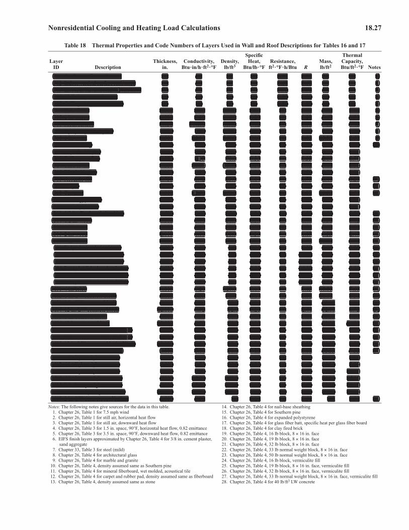
Nonresidential Cooling and Heating Load Calculations 18.27
Table 18 Thermal Properties and Code Numbers of Layers Used in Wall and Roof Descriptions for Tables 16 and 17
Layer ID Description
Thickness, in.
Conductivity, Btu·in/h·ft2·°F
Density, lb/ft3
Specific Heat,
Btu/lb·°FResistance,
ft2 ·°F·h/Btu RMass,lb/ft2
Thermal Capacity, Btu/ft2·°F Notes
F01 Outdoor surface resistance — — — — 0.25 0.25 — — 1F02 Indoor vertical surface resistance — — — — 0.68 0.68 — — 2F03 Indoor horizontal surface resistance — — — — 0.92 0.92 — — 3F04 Wall air space resistance — — — — 0.87 0.87 — — 4F05 Ceiling air space resistance — — — — 1.00 1.00 — — 5F06 EIFS finish 0.375 5.00 116.0 0.20 — 0.08 3.63 0.73 6F07 1 in. stucco 1.000 5.00 116.0 0.20 — 0.20 9.67 1.93 6F08 Metal surface 0.030 314.00 489.0 0.12 — 0.00 1.22 0.15 7F09 Opaque spandrel glass 0.250 6.90 158.0 0.21 — 0.04 3.29 0.69 8F10 1 in. stone 1.000 22.00 160.0 0.19 — 0.05 13.33 2.53 9F11 Wood siding 0.500 0.62 37.0 0.28 — 0.81 1.54 0.43 10F12 Asphalt shingles 0.125 0.28 70.0 0.30 — 0.44 0.73 0.22F13 Built-up roofing 0.375 1.13 70.0 0.35 — 0.33 2.19 0.77F14 Slate or tile 0.500 11.00 120.0 0.30 — 0.05 5.00 1.50F15 Wood shingles 0.250 0.27 37.0 0.31 — 0.94 0.77 0.24F16 Acoustic tile 0.750 0.42 23.0 0.14 — 1.79 1.44 0.20 11F17 Carpet 0.500 0.41 18.0 0.33 — 1.23 0.75 0.25 12F18 Terrazzo 1.000 12.50 160.0 0.19 — 0.08 13.33 2.53 13G01 5/8 in. gyp board 0.625 1.11 50.0 0.26 — 0.56 2.60 0.68G02 5/8 in. plywood 0.625 0.80 34.0 0.29 — 0.78 1.77 0.51G03 1/2 in. fiberboard sheathing 0.500 0.47 25.0 0.31 — 1.06 1.04 0.32 14G04 1/2 in. wood 0.500 1.06 38.0 0.39 — 0.47 1.58 0.62 15G05 1 in. wood 1.000 1.06 38.0 0.39 — 0.94 3.17 1.24 15G06 2 in. wood 2.000 1.06 38.0 0.39 — 1.89 6.33 2.47 15G07 4 in. wood 4.000 1.06 38.0 0.39 — 3.77 12.67 4.94 15I01 R-5, 1 in. insulation board 1.000 0.20 2.7 0.29 — 5.00 0.23 0.07 16I02 R-10, 2 in. insulation board 2.000 0.20 2.7 0.29 — 10.00 0.45 0.13 16I03 R-15, 3 in. insulation board 3.000 0.20 2.7 0.29 — 15.00 0.68 0.20 16I04 R-11, 3-1/2 in. batt insulation 3.520 0.32 1.2 0.23 — 11.00 0.35 0.08 17I05 R-19, 6-1/4 in. batt insulation 6.080 0.32 1.2 0.23 — 19.00 0.61 0.14 17I06 R-30, 9-1/2 in. batt insulation 9.600 0.32 1.2 0.23 — 30.00 0.96 0.22 17
M01 4 in. brick 4.000 6.20 120.0 0.19 — 0.65 40.00 7.60 18M02 6 in. LW concrete block 6.000 3.39 32.0 0.21 — 1.77 16.00 3.36 19M03 8 in. LW concrete block 8.000 3.44 29.0 0.21 — 2.33 19.33 4.06 20M04 12 in. LW concrete block 12.000 4.92 32.0 0.21 — 2.44 32.00 6.72 21M05 8 in. concrete block 8.000 7.72 50.0 0.22 — 1.04 33.33 7.33 22M06 12 in. concrete block 12.000 9.72 50.0 0.22 — 1.23 50.00 11.00 23M07 6 in. LW concrete block (filled) 6.000 1.98 32.0 0.21 — 3.03 16.00 3.36 24M08 8 in. LW concrete block (filled) 8.000 1.80 29.0 0.21 — 4.44 19.33 4.06 25M09 12 in. LW concrete block (filled) 12.000 2.04 32.0 0.21 — 5.88 32.00 6.72 26M10 8 in. concrete block (filled) 8.000 5.00 50.0 0.22 — 1.60 33.33 7.33 27M11 4 in. lightweight concrete 4.000 3.70 80.0 0.20 — 1.08 26.67 5.33M12 6 in. lightweight concrete 6.000 3.70 80.0 0.20 — 1.62 40.00 8.00M13 8 in. lightweight concrete 8.000 3.70 80.0 0.20 — 2.16 53.33 10.67M14 6 in. heavyweight concrete 6.000 13.50 140.0 0.22 — 0.44 70.00 15.05M15 8 in. heavyweight concrete 8.000 13.50 140.0 0.22 — 0.48 93.33 20.07M16 12 in. heavyweight concrete 12.000 13.50 140.0 0.22 — 0.89 140.0 30.10M17 2 in. LW concrete roof ballast 2.000 1.30 40 0.20 — 1.54 6.7 1.33 28
Notes: The following notes give sources for the data in this table.1. Chapter 26, Table 1 for 7.5 mph wind2. Chapter 26, Table 1 for still air, horizontal heat flow3. Chapter 26, Table 1 for still air, downward heat flow4. Chapter 26, Table 3 for 1.5 in. space, 90°F, horizontal heat flow, 0.82 emittance5. Chapter 26, Table 3 for 3.5 in. space, 90°F, downward heat flow, 0.82 emittance6. EIFS finish layers approximated by Chapter 26, Table 4 for 3/8 in. cement plaster,
sand aggregate7. Chapter 33, Table 3 for steel (mild)8. Chapter 26, Table 4 for architectural glass9. Chapter 26, Table 4 for marble and granite
10. Chapter 26, Table 4, density assumed same as Southern pine11. Chapter 26, Table 4 for mineral fiberboard, wet molded, acoustical tile12. Chapter 26, Table 4 for carpet and rubber pad, density assumed same as fiberboard13. Chapter 26, Table 4, density assumed same as stone
14. Chapter 26, Table 4 for nail-base sheathing15. Chapter 26, Table 4 for Southern pine16. Chapter 26, Table 4 for expanded polystyrene17. Chapter 26, Table 4 for glass fiber batt, specific heat per glass fiber board18. Chapter 26, Table 4 for clay fired brick19. Chapter 26, Table 4, 16 lb block, 8 �16 in. face20. Chapter 26, Table 4, 19 lb block, 8 �16 in. face21. Chapter 26, Table 4, 32 lb block, 8 �16 in. face22. Chapter 26, Table 4, 33 lb normal weight block, 8 16 in. face23. Chapter 26, Table 4, 50 lb normal weight block, 8 �16 in. face24. Chapter 26, Table 4, 16 lb block, vermiculite fill25. Chapter 26, Table 4, 19 lb block, 8 �16 in. face, vermiculite fill26. Chapter 26, Table 4, 32 lb block, 8 �16 in. face, vermiculite fill27. Chapter 26, Table 4, 33 lb normal weight block, 8 �16 in. face, vermiculite fill28. Chapter 26, Table 4 for 40 lb/ft3 LW concrete
F01 Outdoor surface resistance — — — — 0.25 0.25 — — 1F02 Indoor vertical surface resistance — — — — 0.68 0.68 — — 2F03 Indoor horizontal surface resistance — — — — 0.92 0.92 — — 3F04 Wall air space resistance — — — — 0.87 0.87 — — 4F05 Ceiling air space resistance — — — — 1.00 1.00 — — 5F06 EIFS finish 0.375 5.00 116.0 0.20 — 0.08 3.63 0.73 6F07 1 in. stucco 1.000 5.00 116.0 0.20 — 0.20 9.67 1.93 6F08 Metal surface 0.030 314.00 489.0 0.12 — 0.00 1.22 0.15 7F09 Opaque spandrel glass 0.250 6.90 158.0 0.21 — 0.04 3.29 0.69 8F10 1 in. stone 1.000 22.00 160.0 0.19 — 0.05 13.33 2.53 9F11 Wood siding 0.500 0.62 37.0 0.28 — 0.81 1.54 0.43 10F12 Asphalt shingles 0.125 0.28 70.0 0.30 — 0.44 0.73 0.22F13 Built-up roofing 0.375 1.13 70.0 0.35 — 0.33 2.19 0.77F14 Slate or tile 0.500 11.00 120.0 0.30 — 0.05 5.00 1.50F15 Wood shingles 0.250 0.27 37.0 0.31 — 0.94 0.77 0.24F16 Acoustic tile 0.750 0.42 23.0 0.14 — 1.79 1.44 0.20 11F17 Carpet 0.500 0.41 18.0 0.33 — 1.23 0.75 0.25 12F18 Terrazzo 1.000 12.50 160.0 0.19 — 0.08 13.33 2.53 13G01 5/8 in. gyp board 0.625 1.11 50.0 0.26 — 0.56 2.60 0.68G02 5/8 in. plywood 0.625 0.80 34.0 0.29 — 0.78 1.77 0.51G03 1/2 in. fiberboard sheathing 0.500 0.47 25.0 0.31 — 1.06 1.04 0.32 14G04 1/2 in. wood 0.500 1.06 38.0 0.39 — 0.47 1.58 0.62 15G05 1 in. wood 1.000 1.06 38.0 0.39 — 0.94 3.17 1.24 15G06 2 in. wood 2.000 1.06 38.0 0.39 — 1.89 6.33 2.47 15G07 4 in. wood 4.000 1.06 38.0 0.39 — 3.77 12.67 4.94 15I01 R-5, 1 in. insulation board 1.000 0.20 2.7 0.29 — 5.00 0.23 0.07 16I02 R-10, 2 in. insulation board 2.000 0.20 2.7 0.29 — 10.00 0.45 0.13 16I03 R-15, 3 in. insulation board 3.000 0.20 2.7 0.29 — 15.00 0.68 0.20 16I04 R-11, 3-1/2 in. batt insulation 3.520 0.32 1.2 0.23 — 11.00 0.35 0.08 17I05 R-19, 6-1/4 in. batt insulation 6.080 0.32 1.2 0.23 — 19.00 0.61 0.14 17I06 R-30, 9-1/2 in. batt insulation 9.600 0.32 1.2 0.23 — 30.00 0.96 0.22 17
M01 4 in. brick 4.000 6.20 120.0 0.19 — 0.65 40.00 7.60 18M02 6 in. LW concrete block 6.000 3.39 32.0 0.21 — 1.77 16.00 3.36 19M03 8 in. LW concrete block 8.000 3.44 29.0 0.21 — 2.33 19.33 4.06 20M04 12 in. LW concrete block 12.000 4.92 32.0 0.21 — 2.44 32.00 6.72 21M05 8 in. concrete block 8.000 7.72 50.0 0.22 — 1.04 33.33 7.33 22M06 12 in. concrete block 12.000 9.72 50.0 0.22 — 1.23 50.00 11.00 23M07 6 in. LW concrete block (filled) 6.000 1.98 32.0 0.21 — 3.03 16.00 3.36 24M08 8 in. LW concrete block (filled) 8.000 1.80 29.0 0.21 — 4.44 19.33 4.06 25M09 12 in. LW concrete block (filled) 12.000 2.04 32.0 0.21 — 5.88 32.00 6.72 26M10 8 in. concrete block (filled) 8.000 5.00 50.0 0.22 — 1.60 33.33 7.33 27M11 4 in. lightweight concrete 4.000 3.70 80.0 0.20 — 1.08 26.67 5.33M12 6 in. lightweight concrete 6.000 3.70 80.0 0.20 — 1.62 40.00 8.00M13 8 in. lightweight concrete 8.000 3.70 80.0 0.20 — 2.16 53.33 10.67M14 6 in. heavyweight concrete 6.000 13.50 140.0 0.22 — 0.44 70.00 15.05M15 8 in. heavyweight concrete 8.000 13.50 140.0 0.22 — 0.48 93.33 20.07M16 12 in. heavyweight concrete 12.000 13.50 140.0 0.22 — 0.89 140.0 30.10M17 2 in. LW concrete roof ballast 2.000 1.30 40 0.20 — 1.54 6.7 1.33 28
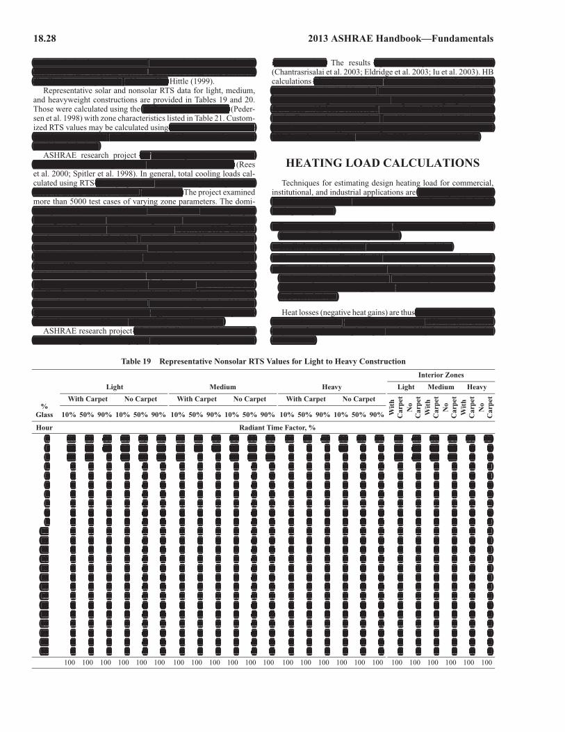
18.28 2013 ASHRAE Handbook—Fundamentals
used. Radiation from those sources is assumed to be more uniformlydistributed onto all room surfaces. Effect of beam solar radiationdistribution assumptions is addressed by Hittle (1999).
Representative solar and nonsolar RTS data for light, medium,and heavyweight constructions are provided in Tables 19 and 20.Those were calculated using the Hbfort computer program (Peder-sen et al. 1998) with zone characteristics listed in Table 21. Custom-ized RTS values may be calculated using the HB method where thezone is not reasonably similar to these typical zones or where moreprecision is desired.
ASHRAE research project RP-942 compared HB and RTSresults over a wide range of zone types and input variables (Reeset al. 2000; Spitler et al. 1998). In general, total cooling loads cal-culated using RTS closely agreed with or were slightly higher thanthose of the HB method with the same inputs. The project examinedmore than 5000 test cases of varying zone parameters. The domi-nating variable was overall thermal mass, and results were groupedinto lightweight, U.S. medium-weight, U.K. medium-weight, andheavyweight construction. Best agreement between RTS and HBresults was obtained for light- and medium-weight construction.Greater differences occurred in heavyweight cases, with RTS gen-erally predicting slightly higher peak cooling loads than HB.Greater differences also were observed in zones with extremelyhigh internal radiant loads and large glazing areas or with a verylightweight exterior envelope. In this case, heat balance calculationspredict that some of the internal radiant load will be transmitted tothe outdoor environment and never becomes cooling load within thespace. RTS does not account for energy transfer out of the space tothe environment, and thus predicted higher cooling loads.
ASHRAE research project RP-1117 built two model rooms forwhich cooling loads were physically measured using extensive
instrumentation. The results agreed with previous simulations(Chantrasrisalai et al. 2003; Eldridge et al. 2003; Iu et al. 2003). HBcalculations closely approximated measured cooling loads whenprovided with detailed data for the test rooms. RTS overpredictedmeasured cooling loads in tests with large, clear, single-glazed win-dow areas with bare concrete floor and no furnishings or internalloads. Tests under more typical conditions (venetian blinds, car-peted floor, office-type furnishings, and normal internal loads) pro-vided good agreement between HB, RTS, and measured loads.
HEATING LOAD CALCULATIONS
Techniques for estimating design heating load for commercial,institutional, and industrial applications are essentially the same asfor those estimating design cooling loads for such uses, with the fol-lowing exceptions:
• Temperatures outdoor conditioned spaces are generally lowerthan maintained space temperatures.
• Credit for solar or internal heat gains is not included• Thermal storage effect of building structure or content is ignored.• Thermal bridging effects on wall and roof conduction are greater
for heating loads than for cooling loads, and greater care must betaken to account for bridging effects on U-factors used in heatingload calculations.
Heat losses (negative heat gains) are thus considered to be instan-taneous, heat transfer essentially conductive, and latent heat treatedonly as a function of replacing space humidity lost to the exteriorenvironment.
Table 19 Representative Nonsolar RTS Values for Light to Heavy Construction
%Glass
Interior Zones
Light Medium Heavy Light Medium Heavy
With Carpet No Carpet With Carpet No Carpet With Carpet No CarpetW
ith
Car
pet
No
Car
pet
Wit
hC
arpe
tN
oC
arpe
tW
ith
Car
pet
No
Car
pet
10% 50% 90% 10% 50% 90% 10% 50% 90% 10% 50% 90% 10% 50% 90% 10% 50% 90%
Hour Radiant Time Factor, %
0 47 50 53 41 43 46 46 49 52 31 33 35 34 38 42 22 25 28 46 40 46 31 33 211 19 18 17 20 19 19 18 17 16 17 16 15 9 9 9 10 9 9 19 20 18 17 9 92 11 10 9 12 11 11 10 9 8 11 10 10 6 6 5 6 6 6 11 12 10 11 6 63 6 6 5 8 7 7 6 5 5 8 7 7 4 4 4 5 5 5 6 8 6 8 5 54 4 4 3 5 5 5 4 3 3 6 5 5 4 4 4 5 5 4 4 5 3 6 4 55 3 3 2 4 3 3 2 2 2 4 4 4 4 3 3 4 4 4 3 4 2 4 4 46 2 2 2 3 3 2 2 2 2 4 3 3 3 3 3 4 4 4 2 3 2 4 3 47 2 1 1 2 2 2 1 1 1 3 3 3 3 3 3 4 4 4 2 2 1 3 3 48 1 1 1 1 1 1 1 1 1 3 2 2 3 3 3 4 3 3 1 1 1 3 3 49 1 1 1 1 1 1 1 1 1 2 2 2 3 3 2 3 3 3 1 1 1 2 3 3
10 1 1 1 1 1 1 1 1 1 2 2 2 3 2 2 3 3 3 1 1 1 2 3 311 1 1 1 1 1 1 1 1 1 2 2 2 2 2 2 3 3 3 1 1 1 2 2 312 1 1 1 1 1 1 1 1 1 1 1 1 2 2 2 3 3 3 1 1 1 1 2 313 1 1 1 0 1 0 1 1 1 1 1 1 2 2 2 3 3 2 1 1 1 1 2 314 0 0 1 0 1 0 1 1 1 1 1 1 2 2 2 3 2 2 1 0 1 1 2 315 0 0 1 0 0 0 1 1 1 1 1 1 2 2 2 2 2 2 0 0 1 1 2 316 0 0 0 0 0 0 1 1 1 1 1 1 2 2 2 2 2 2 0 0 1 1 2 317 0 0 0 0 0 0 1 1 1 1 1 1 2 2 2 2 2 2 0 0 1 1 2 218 0 0 0 0 0 0 1 1 1 1 1 1 2 2 1 2 2 2 0 0 1 1 2 219 0 0 0 0 0 0 0 1 0 0 1 1 2 2 1 2 2 2 0 0 1 0 2 220 0 0 0 0 0 0 0 0 0 0 1 1 2 1 1 2 2 2 0 0 0 0 2 221 0 0 0 0 0 0 0 0 0 0 1 1 2 1 1 2 2 2 0 0 0 0 2 222 0 0 0 0 0 0 0 0 0 0 1 0 1 1 1 2 2 2 0 0 0 0 1 223 0 0 0 0 0 0 0 0 0 0 0 0 1 1 1 2 2 1 0 0 0 0 1 2
100 100 100 100 100 100 100 100 100 100 100 100 100 100 100 100 100 100 100 100 100 100 100 100
used. Radiation from those sources is assumed to be more uniformlydistributed onto all room surfaces. Effect of beam solar radiationdistribution assumptions is addressed by
Hbfort computer program
the HB method where thezone is not reasonably similar to these typical zones or where moreprecision is desired.
RP-942 compared HB and RTSresults over a wide range of zone types and input variables
closely agreed with or were slightly higher thanthose of the HB method with the same inputs. T
nating variable was overall thermal mass, and results were groupedinto lightweight, U.S. medium-weight, U.K. medium-weight, andheavyweight construction. Best agreement between RTS and HBresults was obtained for light- and medium-weight construction.Greater differences occurred in heavyweight cases, with RTS gen-erally predicting slightly higher peak cooling loads than HB.Greater differences also were observed in zones with extremelyhigh internal radiant loads and large glazing areas or with a verylightweight exterior envelope. In this case, heat balance calculationspredict that some of the internal radiant load will be transmitted tothe outdoor environment and never becomes cooling load within thespace. RTS does not account for energy transfer out of the space tothe environment, and thus predicted higher cooling loads.
RP-1117 built two model rooms forwhich cooling loads were physically measured using extensive
instrumentation. agreed with previous simulations
closely approximated measured cooling loads whenprovided with detailed data for the test rooms. RTS overpredictedmeasured cooling loads in tests with large, clear, single-glazed win-dow areas with bare concrete floor and no furnishings or internalloads. Tests under more typical conditions (venetian blinds, car-peted floor, office-type furnishings, and normal internal loads) pro-vided good agreement between HB, RTS, and measured loads.
essentially the same asfor those estimating design cooling loads for such uses, with the fol-lowing exceptions:
• Temperatures outdoor conditioned spaces are generally lowerthan maintained space temperatures.
• Credit for solar or internal heat gains is not included• Thermal storage effect of building structure or content is ignored.• Thermal bridging effects on wall and roof conduction are greater
for heating loads than for cooling loads, and greater care must betaken to account for bridging effects on U-factors used in heatingload calculations.
s considered to be instan-taneous, heat transfer essentially conductive, and latent heat treatedonly as a function of replacing space humidity lost to the exteriorenvironment.
0 47 50 53 41 43 46 46 49 52 31 33 35 34 38 42 22 25 28 46 40 46 31 33 211 19 18 17 20 19 19 18 17 16 17 16 15 9 9 9 10 9 9 19 20 18 17 9 92 11 10 9 12 11 11 10 9 8 11 10 10 6 6 5 6 6 6 11 12 10 11 6 63 6 6 5 8 7 7 6 5 5 8 7 7 4 4 4 5 5 5 6 8 6 8 5 54 4 4 3 5 5 5 4 3 3 6 5 5 4 4 4 5 5 4 4 5 3 6 4 55 3 3 2 4 3 3 2 2 2 4 4 4 4 3 3 4 4 4 3 4 2 4 4 46 2 2 2 3 3 2 2 2 2 4 3 3 3 3 3 4 4 4 2 3 2 4 3 47 2 1 1 2 2 2 1 1 1 3 3 3 3 3 3 4 4 4 2 2 1 3 3 48 1 1 1 1 1 1 1 1 1 3 2 2 3 3 3 4 3 3 1 1 1 3 3 49 1 1 1 1 1 1 1 1 1 2 2 2 3 3 2 3 3 3 1 1 1 2 3 3
10 1 1 1 1 1 1 1 1 1 2 2 2 3 2 2 3 3 3 1 1 1 2 3 311 1 1 1 1 1 1 1 1 1 2 2 2 2 2 2 3 3 3 1 1 1 2 2 312 1 1 1 1 1 1 1 1 1 1 1 1 2 2 2 3 3 3 1 1 1 1 2 313 1 1 1 0 1 0 1 1 1 1 1 1 2 2 2 3 3 2 1 1 1 1 2 314 0 0 1 0 1 0 1 1 1 1 1 1 2 2 2 3 2 2 1 0 1 1 2 315 0 0 1 0 0 0 1 1 1 1 1 1 2 2 2 2 2 2 0 0 1 1 2 316 0 0 0 0 0 0 1 1 1 1 1 1 2 2 2 2 2 2 0 0 1 1 2 317 0 0 0 0 0 0 1 1 1 1 1 1 2 2 2 2 2 2 0 0 1 1 2 218 0 0 0 0 0 0 1 1 1 1 1 1 2 2 1 2 2 2 0 0 1 1 2 219 0 0 0 0 0 0 0 1 0 0 1 1 2 2 1 2 2 2 0 0 1 0 2 220 0 0 0 0 0 0 0 0 0 0 1 1 2 1 1 2 2 2 0 0 0 0 2 221 0 0 0 0 0 0 0 0 0 0 1 1 2 1 1 2 2 2 0 0 0 0 2 222 0 0 0 0 0 0 0 0 0 0 1 0 1 1 1 2 2 2 0 0 0 0 1 223 0 0 0 0 0 0 0 0 0 0 0 0 1 1 1 2 2 1 0 0 0 0 1 2
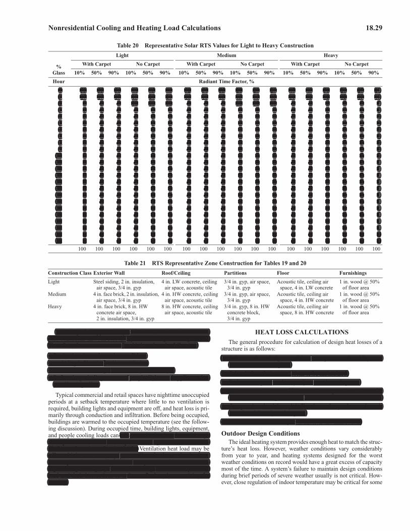
Nonresidential Cooling and Heating Load Calculations 18.29
This simplified approach is justified because it evaluates worst-case conditions that can reasonably occur during a heating season.Therefore, the near-worst-case load is based on the following:
• Design interior and exterior conditions• Including infiltration and/or ventilation• No solar effect (at night or on cloudy winter days)• Before the periodic presence of people, lights, and appliances has
an offsetting effect
Typical commercial and retail spaces have nighttime unoccupiedperiods at a setback temperature where little to no ventilation isrequired, building lights and equipment are off, and heat loss is pri-marily through conduction and infiltration. Before being occupied,buildings are warmed to the occupied temperature (see the follow-ing discussion). During occupied time, building lights, equipment,and people cooling loads can offset conduction heat loss, althoughsome perimeter heat may be required, leaving infiltration and ven-tilation as the primary heating loads. Ventilation heat load may beoffset with heat recovery equipment. These loads (conduction loss,warm-up load, and ventilation load) may not be additive when siz-ing building heating equipment, and it is prudent to analyze eachload and their interactions to arrive at final equipment sizing forheating.
HEAT LOSS CALCULATIONS
The general procedure for calculation of design heat losses of astructure is as follows:
1. Select outdoor design conditions: temperature, humidity, andwind direction and speed.
2. Select indoor design conditions to be maintained.
3. Estimate temperature in any adjacent unheated spaces.
4. Select transmission coefficients and compute heat losses forwalls, floors, ceilings, windows, doors, and foundation elements.
5. Compute heat load through infiltration and any other outdoor airintroduced directly to the space.
6. Sum the losses caused by transmission and infiltration.
Outdoor Design ConditionsThe ideal heating system provides enough heat to match the struc-
ture’s heat loss. However, weather conditions vary considerablyfrom year to year, and heating systems designed for the worstweather conditions on record would have a great excess of capacitymost of the time. A system’s failure to maintain design conditionsduring brief periods of severe weather usually is not critical. How-ever, close regulation of indoor temperature may be critical for some
Table 20 Representative Solar RTS Values for Light to Heavy Construction
%Glass
Light Medium Heavy
With Carpet No Carpet With Carpet No Carpet With Carpet No Carpet
10% 50% 90% 10% 50% 90% 10% 50% 90% 10% 50% 90% 10% 50% 90% 10% 50% 90%
Hour Radiant Time Factor, %
0 53 55 56 44 45 46 52 54 55 28 29 29 47 49 51 26 27 281 17 17 17 19 20 20 16 16 15 15 15 15 11 12 12 12 13 132 9 9 9 11 11 11 8 8 8 10 10 10 6 6 6 7 7 73 5 5 5 7 7 7 5 4 4 7 7 7 4 4 3 5 5 54 3 3 3 5 5 5 3 3 3 6 6 6 3 3 3 4 4 45 2 2 2 3 3 3 2 2 2 5 5 5 2 2 2 4 4 46 2 2 2 3 2 2 2 1 1 4 4 4 2 2 2 3 3 37 1 1 1 2 2 2 1 1 1 4 3 3 2 2 2 3 3 38 1 1 1 1 1 1 1 1 1 3 3 3 2 2 2 3 3 39 1 1 1 1 1 1 1 1 1 3 3 3 2 2 2 3 3 3
10 1 1 1 1 1 1 1 1 1 2 2 2 2 2 2 3 3 311 1 1 1 1 1 1 1 1 1 2 2 2 2 2 1 3 3 212 1 1 1 1 1 0 1 1 1 2 2 2 2 1 1 2 2 213 1 1 0 1 0 0 1 1 1 2 2 2 2 1 1 2 2 214 1 0 0 0 0 0 1 1 1 1 1 1 2 1 1 2 2 215 1 0 0 0 0 0 1 1 1 1 1 1 1 1 1 2 2 216 0 0 0 0 0 0 1 1 1 1 1 1 1 1 1 2 2 217 0 0 0 0 0 0 1 1 1 1 1 1 1 1 1 2 2 218 0 0 0 0 0 0 1 1 1 1 1 1 1 1 1 2 2 219 0 0 0 0 0 0 0 0 0 1 1 1 1 1 1 2 2 220 0 0 0 0 0 0 0 0 0 1 1 1 1 1 1 2 2 221 0 0 0 0 0 0 0 0 0 0 0 0 1 1 1 2 2 222 0 0 0 0 0 0 0 0 0 0 0 0 1 1 1 2 1 123 0 0 0 0 0 0 0 0 0 0 0 0 1 1 1 2 1 1
100 100 100 100 100 100 100 100 100 100 100 100 100 100 100 100 100 100
Table 21 RTS Representative Zone Construction for Tables 19 and 20
Construction Class Exterior Wall Roof/Ceiling Partitions Floor Furnishings
Light Steel siding, 2 in. insulation, air space, 3/4 in. gyp
4 in. LW concrete, ceiling air space, acoustic tile
3/4 in. gyp, air space, 3/4 in. gyp
Acoustic tile, ceiling air space, 4 in. LW concrete
1 in. wood @ 50% of floor area
Medium 4 in. face brick, 2 in. insulation, air space, 3/4 in. gyp
4 in. HW concrete, ceiling air space, acoustic tile
3/4 in. gyp, air space, 3/4 in. gyp
Acoustic tile, ceiling air space, 4 in. HW concrete
1 in. wood @ 50% of floor area
Heavy 4 in. face brick, 8 in. HW concrete air space, 2 in. insulation, 3/4 in. gyp
8 in. HW concrete, ceiling air space, acoustic tile
3/4 in. gyp, 8 in. HW concrete block, 3/4 in. gyp
Acoustic tile, ceiling air space, 8 in. HW concrete
1 in. wood @ 50% of floor area
0 53 55 56 44 45 46 52 54 55 28 29 29 47 49 51 26 27 281 17 17 17 19 20 20 16 16 15 15 15 15 11 12 12 12 13 132 9 9 9 11 11 11 8 8 8 10 10 10 6 6 6 7 7 73 5 5 5 7 7 7 5 4 4 7 7 7 4 4 3 5 5 54 3 3 3 5 5 5 3 3 3 6 6 6 3 3 3 4 4 45 2 2 2 3 3 3 2 2 2 5 5 5 2 2 2 4 4 46 2 2 2 3 2 2 2 1 1 4 4 4 2 2 2 3 3 37 1 1 1 2 2 2 1 1 1 4 3 3 2 2 2 3 3 38 1 1 1 1 1 1 1 1 1 3 3 3 2 2 2 3 3 39 1 1 1 1 1 1 1 1 1 3 3 3 2 2 2 3 3 3
10 1 1 1 1 1 1 1 1 1 2 2 2 2 2 2 3 3 311 1 1 1 1 1 1 1 1 1 2 2 2 2 2 1 3 3 212 1 1 1 1 1 0 1 1 1 2 2 2 2 1 1 2 2 213 1 1 0 1 0 0 1 1 1 2 2 2 2 1 1 2 2 214 1 0 0 0 0 0 1 1 1 1 1 1 2 1 1 2 2 215 1 0 0 0 0 0 1 1 1 1 1 1 1 1 1 2 2 216 0 0 0 0 0 0 1 1 1 1 1 1 1 1 1 2 2 217 0 0 0 0 0 0 1 1 1 1 1 1 1 1 1 2 2 218 0 0 0 0 0 0 1 1 1 1 1 1 1 1 1 2 2 219 0 0 0 0 0 0 0 0 0 1 1 1 1 1 1 2 2 220 0 0 0 0 0 0 0 0 0 1 1 1 1 1 1 2 2 221 0 0 0 0 0 0 0 0 0 0 0 0 1 1 1 2 2 222 0 0 0 0 0 0 0 0 0 0 0 0 1 1 1 2 1 123 0 0 0 0 0 0 0 0 0 0 0 0 1 1 1 2 1 1
This simplified approach is justified because it evaluates worst-case conditions that can reasonably occur during a heating season.Therefore, the near-worst-case load is based on the following:
• Design interior and exterior conditions• Including infiltration and/or ventilation• No solar effect (at night or on cloudy winter days)t• Before the periodic presence of people, lights, and appliances has
an offsetting effect
offset conduction heat loss, althoughtsome perimeter heat may be required, leaving infiltration and ven-tilation as the primary heating loads. offset with heat recovery equipment. These loads (conduction loss,warm-up load, and ventilation load) may not be additive when siz-ing building heating equipment, and it is prudent to analyze eachrrload and their interactions to arrive at final equipment sizing forrrheating.
1. Select outdoor design conditions: temperature, humidity, andwind direction and speed.
2. Select indoor design conditions to be maintained.
3. Estimate temperature in any adjacett nt unheated spaces.
4. Select transmission coefficients and compute heat losses forwalls, floors, ceilings, windows, doors, and foundation elements.
5. Compute heat load through infiltration and any other outdoor airintroduced directly to the space.
6. Sum the losses caused by transmission and infiltration.
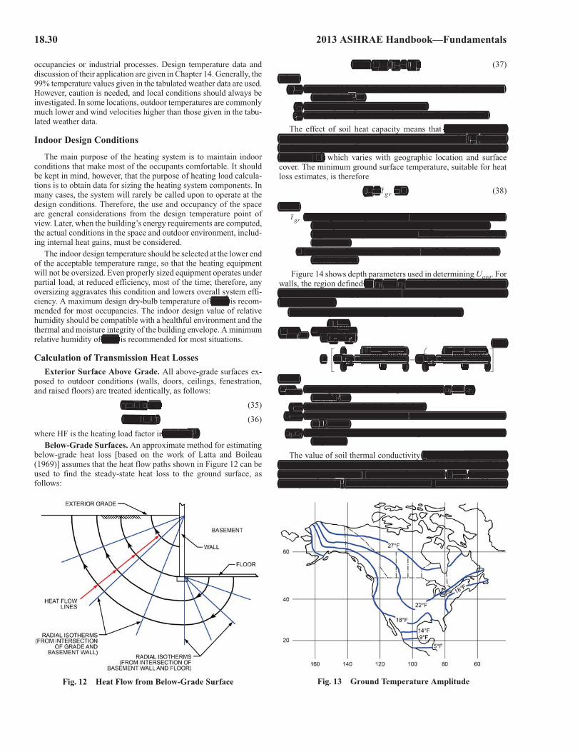
18.30 2013 ASHRAE Handbook—Fundamentals
occupancies or industrial processes. Design temperature data anddiscussion of their application are given in Chapter 14. Generally, the99% temperature values given in the tabulated weather data are used.However, caution is needed, and local conditions should always beinvestigated. In some locations, outdoor temperatures are commonlymuch lower and wind velocities higher than those given in the tabu-lated weather data.
Indoor Design Conditions
The main purpose of the heating system is to maintain indoorconditions that make most of the occupants comfortable. It shouldbe kept in mind, however, that the purpose of heating load calcula-tions is to obtain data for sizing the heating system components. Inmany cases, the system will rarely be called upon to operate at thedesign conditions. Therefore, the use and occupancy of the spaceare general considerations from the design temperature point ofview. Later, when the building’s energy requirements are computed,the actual conditions in the space and outdoor environment, includ-ing internal heat gains, must be considered.
The indoor design temperature should be selected at the lower endof the acceptable temperature range, so that the heating equipmentwill not be oversized. Even properly sized equipment operates underpartial load, at reduced efficiency, most of the time; therefore, anyoversizing aggravates this condition and lowers overall system effi-ciency. A maximum design dry-bulb temperature of 70°F is recom-mended for most occupancies. The indoor design value of relativehumidity should be compatible with a healthful environment and thethermal and moisture integrity of the building envelope. A minimumrelative humidity of 30% is recommended for most situations.
Calculation of Transmission Heat Losses
Exterior Surface Above Grade. All above-grade surfaces ex-posed to outdoor conditions (walls, doors, ceilings, fenestration,and raised floors) are treated identically, as follows:
q = A HF (35)
HF = U t (36)
where HF is the heating load factor in Btu/h·ft2.Below-Grade Surfaces. An approximate method for estimating
below-grade heat loss [based on the work of Latta and Boileau(1969)] assumes that the heat flow paths shown in Figure 12 can beused to find the steady-state heat loss to the ground surface, asfollows:
HF = Uavg (tin – tgr) (37)
whereUavg = average U-factor for below-grade surface from Equation (39) or
(40), Btu/h·ft2·°Ftin = below-grade space air temperature, °Ftgr = design ground surface temperature from Equation (38), °F
The effect of soil heat capacity means that none of the usualexternal design air temperatures are suitable values for tgr. Groundsurface temperature fluctuates about an annual mean value byamplitude A, which varies with geographic location and surfacecover. The minimum ground surface temperature, suitable for heatloss estimates, is therefore
tgr = – A (38)
where= mean ground temperature, °F, estimated from the annual average
air temperature or from well-water temperatures, shown in Figure 17 of Chapter 34 in the 2011 ASHRAE Handbook—HVAC Applications
A = ground surface temperature amplitude, °F, from Figure 13 for North America
Figure 14 shows depth parameters used in determining Uavg. Forwalls, the region defined by z1 and z2 may be the entire wall or anyportion of it, allowing partially insulated configurations to be ana-lyzed piecewise.
The below-grade wall average U-factor is given by
(39)
whereUavg,bw = average U-factor for wall region defined by z1 and z2,
Btu/h·ft2·°Fksoil = soil thermal conductivity, Btu/h·ft·°F
Rother = total resistance of wall, insulation, and indoor surface resistance, h·ft2·°F/Btu
z1, z2 = depths of top and bottom of wall segment under consideration, ft (Figure 14)
The value of soil thermal conductivity k varies widely with soiltype and moisture content. A typical value of 0.8 Btu/h·ft·°F hasbeen used previously to tabulate U-factors, and Rother is approxi-mately 1.47 h · ft2 · °F/Btu for uninsulated concrete walls. For
Fig. 12 Heat Flow from Below-Grade Surface
t gr
t gr
Fig. 13 Ground Temperature Amplitude
Uavg ,bw
2ksoil
� z2 z1–� �------------------------=
× ln z2
2ksoilRother
�-----------------------------+
� �� �� �
ln z1
2ksoilRother
�-----------------------------+
� �� �� �
–
f 70°F
f 30%
q = A HF
HF = U t
ft2./h·fn BBtu/
HF = UavgUU g ((tin – tgrt )
whereUavgUU = average U-factor for below-grade surface from Equation (39) or
ft2(40), Btu/h·f 2·°Ftin = below-grade space air temperature, °Ftgrt = design ground surface temperature from Equation (38), °F
none of the usualexternal design air temperatures are suitable values for tgrt . Groundgrsurface temperature fluctuates about an annual mean value byamplitude A,
tgrt r = – A
where= mean ground temperature, °F, estimated from the annual average
air temperature or from well-water temperatures, shown inFigure 17 of Chapter 34 in the 2011 ASHRAE Handbook—HVAC Applications
A = ground surface temperature amplitude, °F, from Figure 13 for North America
d by z1 and z2 avg
may be the entire wall or any1 2portion of it, allowing partially insulated configurations to be ana-lyzed piecewise.
The below-grade wall average U-factor is given by
(39)
whereUavg,UU = average U-factor for wall region defined by z1 and z2, g,bw g
ft2Btu/h·f 2·°Fksoilk = soil thermal conductivity, Btu/h·ft·°F
Rother = total resistance of wall, insulation, and indoor surface resistance,ft2h·f 2·°F/Btu
z1, z2 = depths of top and bottom of wall segment under consideration, ft(Figure 14)
2ksoilkUavgU ,
soil----------------------------=,bw �� 2�z2
------–-----
1z1------�1
� 2ksoilk Rother�r �2ksoilk Rother× ln�
��� 2z22
��
soil other-----------------------------+
�soil other��
soil otherln���� 1z11
��
soil other-----------------------------+
�soil other��
soil other
� ���z�� �
��� �
�z�� �
���
k varies widely with soilktype and moisture content. A typical value of 0.8 Btu/h·ft·°F hasbeen used previously to tabulate U-factors, and Rother r is approxi-
ft2mately 1.47 h · fother
2 · °F/Btu for uninsulated concrete walls. For
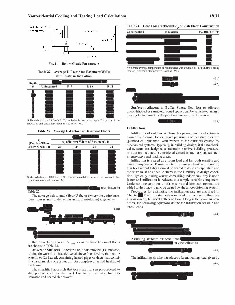
Nonresidential Cooling and Heating Load Calculations 18.31
these parameters, representative values for Uavg,bw are shown inTable 22.
The average below-grade floor U-factor (where the entire base-ment floor is uninsulated or has uniform insulation) is given by
(40)
wherewb = basement width (shortest dimension), ftzf = floor depth below grade, ft (see Figure 14)
Representative values of Uavg,bf for uninsulated basement floorsare shown in Table 23.
At-Grade Surfaces. Concrete slab floors may be (1) unheated,relying for warmth on heat delivered above floor level by the heatingsystem, or (2) heated, containing heated pipes or ducts that consti-tute a radiant slab or portion of it for complete or partial heating ofthe house.
The simplified approach that treats heat loss as proportional toslab perimeter allows slab heat loss to be estimated for bothunheated and heated slab floors:
q = p HF (41)
HF = Fp t (42)
whereq = heat loss through perimeter, Btu/h
Fp = heat loss coefficient per foot of perimeter, Btu/h·ft·°F, Table 24p = perimeter (exposed edge) of floor, ft
Surfaces Adjacent to Buffer Space. Heat loss to adjacentunconditioned or semiconditioned spaces can be calculated using aheating factor based on the partition temperature difference:
HF = U (tin – tb) (43)
InfiltrationInfiltration of outdoor air through openings into a structure is
caused by thermal forces, wind pressure, and negative pressure(planned or unplanned) with respect to the outdoors created bymechanical systems. Typically, in building design, if the mechani-cal systems are designed to maintain positive building pressure,infiltration need not be considered except in ancillary spaces suchas entryways and loading areas.
Infiltration is treated as a room load and has both sensible andlatent components. During winter, this means heat and humidityloss because cold, dry air must be heated to design temperature andmoisture must be added to increase the humidity to design condi-tion. Typically, during winter, controlling indoor humidity is not afactor and infiltration is reduced to a simple sensible component.Under cooling conditions, both sensible and latent components areadded to the space load to be treated by the air conditioning system.
Procedures for estimating the infiltration rate are discussed inChapter 16. The infiltration rate is reduced to a volumetric flow rateat a known dry bulb/wet bulb condition. Along with indoor air con-dition, the following equations define the infiltration sensible andlatent loads.
qs (Btu/h) = 60(cfm/v) cp (tin – to) (44)
wherecfm = volume flow rate of infiltrating air
cp = specific heat capacity of air, Btu/lbm·ºFv = specific volume of infiltrating air, ft3/lbm
Assuming standard air conditions (59°F and sea-level condi-tions) for v and cp, Equation (44) may be written as
qs (Btu/h) = 1.10(cfm)(tin – to) (45)
The infiltrating air also introduces a latent heating load given by
ql = 60(cfm/v)(Win – Wo)Dh (46)
whereWin = humidity ratio for indoor space air, lbw /lbaWo = humidity ratio for outdoor air, lbw/lba
Table 22 Average U-Factor for Basement Walls with Uniform Insulation
Depth,ft
Uavg,bw from Grade to Depth, Btu/h·ft2·°F
Uninsulated R-5 R-10 R-15
1 0.432 0.135 0.080 0.0572.6 0.331 0.121 0.075 0.0543 0.273 0.110 0.070 0.0524 0.235 0.101 0.066 0.0505 0.208 0.094 0.063 0.0486 0.187 0.088 0.060 0.0467 0.170 0.083 0.057 0.0448 0.157 0.078 0.055 0.043
Soil conductivity = 0.8 Btu/h·ft ·°F; insulation is over entire depth. For other soil con-ductivities and partial insulation, use Equation (39).
Table 23 Average U-Factor for Basement Floors
zf(Depth of FloorBelow Grade), ft
Uavg,bf , Btu/h·ft2·°F
wb (Shortest Width of Basement), ft
20 24 28 32
1 0.064 0.057 0.052 0.0472 0.054 0.048 0.044 0.0403 0.047 0.042 0.039 0.0364 0.042 0.038 0.035 0.0335 0.038 0.035 0.032 0.0306 0.035 0.032 0.030 0.0287 0.032 0.030 0.028 0.026
Soil conductivity is 0.8 Btu/h·ft ·°F; floor is uninsulated. For other soil conductivitiesand insulation, use Equation (39).
Fig. 14 Below-Grade Parameters
Uavg bf,
2ksoil
�wb--------------=
× wb
2------
zf
2---+
ksoil Rother
�---------------------------+
� �� �� �
lnzf
2---
ksoil Rother
�---------------------------+� �
� �ln–
Table 24 Heat Loss Coefficient Fp of Slab Floor Construction
Construction Insulation Fp , Btu/h·ft·°F
8 in. block wall, brick facing Uninsulated 0.68R-5.4 from edge to footer 0.50
4 in. block wall, brick facing Uninsulated 0.84R-5.4 from edge to footer 0.49
Metal stud wall, stucco Uninsulated 1.20R-5.4 from edge to footer 0.53
Poured concrete wall with duct near perimeter*
Uninsulated 2.12R-5.4 from edge to footer 0.72
*Weighted average temperature of heating duct was assumed at 110ºF during heatingseason (outdoor air temperature less than 65ºF).
these parameters, representative values for Uavg,UU g,bw
1 0.064 0.057 0.052 0.0472 0.054 0.048 0.044 0.0403 0.047 0.042 0.039 0.0364 0.042 0.038 0.035 0.0335 0.038 0.035 0.032 0.0306 0.035 0.032 0.030 0.0287 0.032 0.030 0.028 0.026
ft2Uavg,UU f , Btu/h·f 2·°Fg,bf
1 0.432 0.135 0.080 0.0572.6 0.331 0.121 0.075 0.0543 0.273 0.110 0.070 0.0524 0.235 0.101 0.066 0.0505 0.208 0.094 0.063 0.0486 0.187 0.088 0.060 0.0467 0.170 0.083 0.057 0.0448 0.157 0.078 0.055 0.043
ft2Uavg,UU from Grade to Depth, Btu/h·f 2·°Fg,bw
8 in. block wall, brick facing Uninsulated 0.68R-5.4 from edge to footer 0.50
4 in. block wall, brick facing Uninsulated 0.84R-5.4 from edge to footer 0.49
Metal stud wall, stucco Uninsulated 1.20R-5.4 from edge to footer 0.53
Poured concrete wall with Uninsulated 2.12duct near perimeter* R-5.4 from edge to footer 0.72
2ksoilkUavgU
soil------------------=bf ��wb
---------
� �zfzzfz �ksoilk Rotherksoilk Rother zfz k Rksoilk Rother�wbwb �z �r× ����w
ln ��r��r �ln–
wb------f
---+soil other
---------------------------++ +wb f soil other
--- ---------------------------+� �f soil other+
f+�-
���n �--
����
��� 2------2 2
---2 � �
��� 2� 2
---��
wherewb = basement width (shortest dimension), ftzfz = floor depth below grade, ft (see Figure 14)
q = p HF
HF = Fp FF t
whereq = heat loss through perimeter, Btu/h
FpFF = heat loss coefficient per foot of perimeter, Btu/h·ft·°F, Table 24pp = perimeter (exposed edge) of floor, ft
HF = U ((tin – tbt )
r 16. T
qs (Btu/h) = 60(cfm/v) cpc ((tin – to)
wherecfm = volume flow rate of infiltrating air
cpc = specific heat capacity of air, Btu//lbmm·ºFmft3/
pv = specific volume of infiltrating air, /lbm
(59°F and sea-level condi-tions) for v and cpc , Equation (44)
qs (Btu/h) = 1.10(cfm)((tin – to)
ql l = 60(cfm/v)((WinWW – WoWW )Dh
whereWinWW = humidity ratio for indoor space air, lbw /lbaWoWW = humidity ratio for outdoor air, lbw/lba
18.32 2013 ASHRAE Handbook—Fundamentals
Dh = change in enthalpy to convert 1 lb water from vapor to liquid, Btu/lbw
For standard air and nominal indoor comfort conditions, thelatent load may be expressed as
ql = 4840(cfm)(Win – Wo) (47)
The coefficients 1.10 in Equation (45) and 4840 in Equation (47)are given for standard conditions. They depend on temperature andaltitude (and, consequently, pressure).
HEATING SAFETY FACTORS AND LOAD ALLOWANCES
Before mechanical cooling became common in the second half ofthe 1900s, and when energy was less expensive, buildings includedmuch less insulation; large, operable windows; and generally moreinfiltration-prone assemblies than the energy-efficient and muchtighter buildings typical of today. Allowances of 10 to 20% of the netcalculated heating load for piping losses to unheated spaces, and 10to 20% more for a warm-up load, were common practice, along withother occasional safety factors reflecting the experience and/or con-cern of the individual designer. Such measures are less conserva-tively applied today with newer construction. A combined warm-up/safety allowance of 20 to 25% is fairly common but varies dependingon the particular climate, building use, and type of construction.Engineering judgment must be applied for the particular project.Armstrong et al. (1992a, 1992b) provide a design method to dealwith warm-up and cooldown load.
OTHER HEATING CONSIDERATIONS
Calculation of design heating load estimates has essentiallybecome a subset of the more involved and complex estimation ofcooling loads for such spaces. Chapter 19 discusses using the heat-ing load estimate to predict or analyze energy consumption overtime. Special provisions to deal with particular applications are cov-ered in the 2011 ASHRAE Handbook—HVAC Applications and the2012 ASHRAE Handbook—HVAC Systems and Equipment.
The 1989 ASHRAE Handbook—Fundamentals was the last edi-tion to contain a chapter dedicated only to heating load. Its contentswere incorporated into this volume’s Chapter 17, which describessteady-state conduction and convection heat transfer and provides,among other data, information on losses through basement floorsand slabs.
SYSTEM HEATING AND COOLING LOAD EFFECTS
The heat balance (HB) or radiant time series (RTS) methods areused to determine cooling loads of rooms within a building, but theydo not address the plant size necessary to reject the heat. Principalfactors to consider in determining the plant size are ventilation, heattransport equipment, and air distribution systems. Some of thesefactors vary as a function of room load, ambient temperature, andcontrol strategies, so it is often necessary to evaluate the factors andstrategies dynamically and simultaneously with the heat loss or gaincalculations.
Detailed analysis of system components and methods calculatingtheir contribution to equipment sizing are beyond the scope of thischapter, which is general in nature. Table 25 lists the most fre-quently used calculations in other chapters and volumes.
ZONING
The organization of building rooms as defined for load calcula-tions into zones and air-handling units has no effect on room cooling
loads. However, specific grouping and ungrouping of rooms intozones may cause peak system loads to occur at different timesduring the day or year and may significantly affected heat removalequipment sizes.
For example, if each room is cooled by a separate heat removalsystem, the total capacity of the heat transport systems equals thesum of peak room loads. Conditioning all rooms by a single heattransport system (e.g., a variable-volume air handler) requires lesscapacity (equal to the simultaneous peak of the combined roomsload, which includes some rooms at off-peak loads). This may sig-nificantly reduce equipment capacity, depending on the configura-tion of the building.
VENTILATION
Consult ASHRAE Standard 62.1 and building codes to deter-mine the required quantity of ventilation air for an application, andthe various methods of achieving acceptable indoor air quality. Thefollowing discussion is confined to the effect of mechanical venti-lation on sizing heat removal equipment. Where natural ventilationis used, through operable windows or other means, it is consideredas infiltration and is part of the direct-to-room heat gain. Whereventilation air is conditioned and supplied through the mechanicalsystem, its sensible and latent loads are applied directly to heattransport and central equipment, and do not affect room heating andcooling loads. If the mechanical ventilation rate sufficiently exceedsexhaust airflows, air pressure may be positive and infiltration fromenvelope openings and outdoor wind may not be included in theload calculations. Chapter 16 includes more information on venti-lating commercial buildings.
AIR HEAT TRANSPORT SYSTEMS
Heat transport equipment is usually selected to provide adequateheating or cooling for the peak load condition. However, selectionmust also consider maintaining desired indoor conditions during alloccupied hours, which requires matching the rate of heat transportto room peak heating and cooling loads. Automatic control systemsnormally vary the heating and cooling system capacity during theseoff-peak hours of operation.
On/Off Control SystemsOn/off control systems, common in residential and light com-
mercial applications, cycle equipment on and off to match roomload. They are adaptable to heating or cooling because they cancycle both heating and cooling equipment. In their purest form, theirheat transport matches the combined room and ventilation load overa series of cycles.
Variable-Air-Volume SystemsVariable-air-volume (VAV) systems have airflow controls that
adjust cooling airflow to match the room cooling load. Damper
Table 25 Common Sizing Calculations in Other Chapters
Subject Volume/Chapter Equation(s)
Duct heat transfer ASTM Standard C680Piping heat transfer Fundamentals Ch. 3 (35)Fan heat transfer Fundamentals Ch. 19 (22)Pump heat transfer Systems Ch. 44 (3), (4), (5)Moist-air sensible heating and cooling Fundamentals Ch. 1 (43)Moist-air cooling and dehumidification Fundamentals Ch. 1 (45)Air mixing Fundamentals Ch. 1 (46)Space heat absorption and moist-air
moisture gainsFundamentals Ch. 1 (48)
Adiabatic mixing of water injected into moist air
Fundamentals Ch. 1 (47)
Dh = change in enthalpy to convert 1 lb water from vapor to liquid,Btu//lbw
ql l = 4840(cfm)((WinWW – WoWW )
1.10 d 4840 in temperature and
altitude (and, consequently, pressure).
Duct heat transfer ASTM Standard C680dPiping heat transfer Fundamentals Ch. 3 (35)Fan heat transfer Fundamentals Ch. 19 (22)Pump heat transfer Systems Ch. 44 (3), (4), (5)Moist-air sensible heating and cooling Fundamentals Ch. 1 (43)Moist-air cooling and dehumidification Fundamentals Ch. 1 (45)Air mixing Fundamentals Ch. 1 (46)Space heat absorption and moist-air Fundamentals Ch. 1 (48)
moisture gainsAdiabatic mixing of water injected into Fundamentals Ch. 1 (47)
moist air
f 20 to 25% i t varies dependingon the particular climate, building use, and type of construction.
o determine cooling loads of rooms within a building, but theyfdo not address the plant size necessary to reject the heat.
e ventilation, heattransport equipment, and air distribution systems. Some of thesefactors vary as a function of room load, ambient temperature, andcontrol strategies, so it is often necessary to evaluate the factors andstrategies dynamically and simultaneously with the heat loss or gaincalculations.
62.1
, air pressure may be positive and infiltration fromenvelope openings and outdoor wind may not be included in theload calculations.
are applied directly to heattransport and central equipment, and do not affect room heating andcooling loads. I
it is consideredas infiltration and is part of the direct-to-room heat gain.
matching the rate of heat transportto room peak heating and cooling loads.
, theirheat transport matches the combined room and ventilation load overa series of cycles.
Variable-Air-Volume Variable-air-volume (VAV) systems have airflow controls that
adjust cooling airflow to match the room cooling load. Damper
Nonresidential Cooling and Heating Load Calculations 18.33
leakage or minimum airflow settings may cause overcooling, somost VAV systems are used in conjunction with separate heatingsystems. These may be duct-mounted heating coils, or separate radi-ant or convective heating systems.
The amount of heat added by the heating systems during coolingbecomes part of the room cooling load. Calculations must deter-mine the minimum airflow relative to off-peak cooling loads. Thequantity of heat added to the cooling load can be determined foreach terminal by Equation (9) using the minimum required supplyairflow rate and the difference between supply air temperature andthe room indoor heating design temperature.
Constant-Air-Volume Reheat SystemsIn constant-air-volume (CAV) reheat systems, all supply air is
cooled to remove moisture and then heated to avoid overcoolingrooms. Reheat refers to the amount of heat added to cooling supplyair to raise the supply air temperature to the temperature necessaryfor picking up the sensible load. The quantity of heat added can bedetermined by Equation (9).
With a constant-volume reheat system, heat transport systemload does not vary with changes in room load, unless the coolingcoil discharge temperature is allowed to vary. Where a minimumcirculation rate requires a supply air temperature greater than theavailable design supply air temperature, reheat adds to the coolingload on the heat transport system. This makes the cooling load onthe heat transport system larger than the room peak load.
Mixed Air SystemsMixed air systems change the supply air temperature to match
the cooling capacity by mixing airstreams of different temperatures;examples include multizone and dual-duct systems. Systems thatcool the entire airstream to remove moisture and to reheat some ofthe air before mixing with the cooling airstream influence load onthe heat transport system in the same way a reheat system does.Other systems separate the air paths so that mixing of hot- and cold-deck airstreams does not occur. For systems that mix hot and coldairstreams, the contribution to the heat transport system load isdetermined as follows.
1. Determine the ratio of cold-deck flow to hot-deck flow from
= (Tc – Tr)/(Tr – Th)
2. From Equation (10), the hot-deck contribution to room load dur-ing off-peak cooling is
qrh = 1.1Qh(Th – Tr)
whereQh = heating airflow, cfmQc = cooling airflow, cfmTc = cooling air temperature, °FTh = heating air temperature, °FTr = room or return air temperature, °F
qrh = heating airflow contribution to room load at off-peak hours, Btu/h
Heat Gain from FansFans that circulate air through HVAC systems add energy to the
system through the following processes:
• Increasing velocity and static pressure adds kinetic and potentialenergy
• Fan inefficiency in producing airflow and static pressure addssensible heat (fan heat) to the airflow
• Inefficiency of motor and drive dissipates sensible heat
The power required to provide airflow and static pressure can bedetermined from the first law of thermodynamics with the followingequation:
PA = 0.000157Vp
wherePA = air power, hpV = flow rate, cfmp = pressure, in. of water
at standard air conditions with air density = 0.075 lb/ft3 built into themultiplier 0.000157. The power necessary at the fan shaft mustaccount for fan inefficiencies, which may vary from 50 to 70%. Thismay be determined from
PF = PA /�F
wherePF = power required at fan shaft, hp�F = fan efficiency, dimensionless
The power necessary at the input to the fan motor must account forfan motor inefficiencies and drive losses. Fan motor efficienciesgenerally vary from 80 to 95%, and drive losses for a belt drive are3% of the fan power. This may be determined from
PM = (1 + DL) PF /EM ED
wherePM = power required at input to motor, hpED = belt drive efficiency, dimensionlessEM = fan motor efficiency, dimensionlessPF = power required at fan shaft, hp
DL = drive loss, dimensionless
Almost all the energy required to generate airflow and static pressureis ultimately dissipated as heat within the building and HVAC sys-tem; a small portion is discharged with any exhaust air. Generally, itis assumed that all the heat is released at the fan rather than dispersedto the remainder of the system. The portion of fan heat released to theairstream depends on the location of the fan motor and drive: if theyare within the airstream, all the energy input to the fan motor isreleased to the airstream. If the fan motor and drive are outdoor theairstream, the energy is split between the airstream and the roomhousing the motor and drive. Therefore, the following equations maybe used to calculate heat generated by fans and motors:
If motor and drive are outside the airstream,
qf s = 2545PF
qfr = 2545(PM – PF )
If motor and drive are inside the airstream,
qf s = 2545PM
qfr = 0.0
wherePF = power required at fan shaft, hpPM = power required at input to motor, hpqf s = heat release to airstream, Btu/hqfr = heat release to room housing motor and drive, Btu/h
2545 = conversion factor, Btu/h·hp
Supply airstream temperature rise may be determined from psy-chrometric formulas or Equation (9).
Variable- or adjustable-frequency drives (VFDs or AFDs) oftendrive fan motors in VAV air-handling units. These devices releaseheat to the surrounding space. Refer to manufacturers’ data for heatreleased or efficiencies. The disposition of heat released is deter-mined by the drive’s location: in the conditioned space, in the return
Qh
Qc------
leakage or minimum airflow settings may cause overcooling, somost VAV systems are used in conjunction with separate heatingsystems. These may be duct-mounted heating coils, or separate radi-rant or convective heating systems.
The amount of heat added by the heating systems during coolingbecomes part of the room cooling load. Calculations must deter-mine the minimum airflow relative to off-peak cooling loads. Thequantity of heat added to the cooling load can be determined foreach terminal by Equation (9) using the minimum required supplyairflow rate and the difference between supply air temperature andthe room indoor heating design temperature.
Constant-Air-Volume Reheat In constant-air-volume (CAV) reheat systems, all supply air is
cooled to remove moisture and then heated to avoid overcoolingrooms. Reheat refers to the amount of heat added to cooling supplytair to raise the supply air temperature to the temperature necessaryfor picking up the sensible load. The quantity of heat added can bedetermined by Equation (9).
With a constant-volume reheat system, heat transport systemload does not vary with changes in room load, unless the coolingcoil discharge temperature is allowed to vary. Where a minimumcirculation rate requires a supply air temperature greater than theavailable design supply air temperature, reheat adds to the coolingttload on the heat transport system. This makes the cooling load onthe heat transport system larger than the room peak load.
Mixed Air Mixed air systems change the supply air temperature to match
the cooling capacity by mixing airstreams of different temperatures;examples include multizone and dual-duct systems. Systems thatcool the entire airstream to remove moisture and to reheat some ofthe air before mixing with the cooling airstream influence load onthe heat transport system in the same way a reheat system does.Other systems separate the air paths so that mixing of hot- and cold-deck airstreams does not occur. For systems that mix hot and coldairstreams, the contribution to the heat transport system load isdetermined as follows.
Qc------ = ((TcTT – TrTT )/(TrTT r – ThTT )Qh
qrh = 1.1Qh(ThTT – TrTT )
whereQh = heating airflow, cfmQc = cooling airflow, cfmTcTT = cooling air temperature, °FThTT = heating air temperature, °FTrTT = room or return air temperature, °F
qrh = heating airflow contribution to room load at off-peak hours, Btu/h
• Increasing velocity and static pressure adds kinetic and potentialenergy
• Fan inefficiency in producing airflow and static pressure addssensible heat (fan heat) to the airflow
• Inefficiency of motor and drive dissipates sensible heat
P = 0.000157VpPAPP
whereP = air power, hpPAPPV = flow rate, cfmp = pressure, in. of water
ft3 at standard air conditions with air density = 0.075 lb/f built into themultiplier 0.000157. The power necessary at the fan shaft mustaccount for fan inefficiencies, which may vary from 50 to 70%. Thismay be determined from
P = P /�PFPP PAPP �F
whereP = power required at fan shaft, hpPFPP� = fan efficiency, dimensionless�F
18.34 2013 ASHRAE Handbook—Fundamentals
air path, or in a nonconditioned equipment room. These drives, andother electronic equipment such as building control, data process-ing, and communications devices, are temperature sensitive, so therooms in which they are housed require cooling, frequently year-round.
Duct Surface Heat TransferHeat transfer across the duct surface is one mechanism for
energy transfer to or from air inside a duct. It involves conductionthrough the duct wall and insulation, convection at inner and outersurfaces, and radiation between the duct and its surroundings.Chapter 4 presents a rigorous analysis of duct heat loss and gain,and Chapter 23 addresses application of analysis to insulated ductsystems.
The effect of duct heat loss or gain depends on the duct routing,duct insulation, and its surrounding environment. Consider the fol-lowing conditions:
• For duct run within the area cooled or heated by air in the duct,heat transfer from the space to the duct has no effect on heating orcooling load, but beware of the potential for condensation on coldducts.
• For duct run through unconditioned spaces or outdoors, heattransfer adds to the cooling or heating load for the air transportsystem but not for the conditioned space.
• For duct run through conditioned space not served by the duct,heat transfer affects the conditioned space as well as the air trans-port system serving the duct.
• For an extensive duct system, heat transfer reduces the effectivesupply air differential temperature, requiring adjustment throughair balancing to increase airflow to extremities of the distributionsystem.
Duct LeakageAir leakage from supply ducts can considerably affect HVAC
system energy use. Leakage reduces cooling and/or dehumidifyingcapacity for the conditioned space, and must be offset by increasedairflow (sometimes reduced supply air temperatures), unless leakedair enters the conditioned space directly. Supply air leakage into aceiling return plenum or leakage from unconditioned spaces intoreturn ducts also affects return air temperature and/or humidity.
Determining leakage from a duct system is complex because ofthe variables in paths, fabrication, and installation methods. Refer toChapter 21 and publications from the Sheet Metal and Air Condi-tioning Contractors’ National Association (SMACNA) for methodsof determining leakage. In general, good-quality ducts and post-installation duct sealing provide highly cost-effective energy sav-ings, with improved thermal comfort and delivery of ventilation air.
Ceiling Return Air Plenum TemperaturesThe space above a ceiling, when used as a return air path, is a
ceiling return air plenum, or simply a return plenum. Unlike a tra-ditional ducted return, the plenum may have multiple heat sourcesin the air path. These heat sources may be radiant and convectiveloads from lighting and transformers; conduction loads from adja-cent walls, roofs, or glazing; or duct and piping systems within theplenum.
As heat from these sources is picked up by the unducted returnair, the temperature differential between the ceiling cavity and con-ditioned space is small. Most return plenum temperatures do not risemore than 1 to 3°F above space temperature, thus generating only arelatively small thermal gradient for heat transfer through plenumsurfaces, except to the outdoors. This yields a relatively large-percentage reduction in space cooling load by shifting plenum loadsto the system. Another reason plenum temperatures do not rise more
is leakage into the plenum from supply air ducts, and, if exposed tothe roof, increasing levels of insulation.
Where the ceiling space is used as a return air plenum, energybalance requires that heat picked up from the lights into the returnair (1) become part of the cooling load to the return air (representedby a temperature rise of return air as it passes through the ceilingspace), (2) be partially transferred back into the conditioned spacethrough the ceiling material below, and/or (3) be partially lost fromthe space through floor surfaces above the plenum. If the plenumhas one or more exterior surfaces, heat gains through them must beconsidered; if adjacent to spaces with different indoor temperatures,partition loads must be considered, too. In a multistory building, theconditioned space frequently gains heat through its floor from asimilar plenum below, offsetting the floor loss. The radiant compo-nent of heat leaving the ceiling or floor surface of a plenum is nor-mally so small, because of relatively small temperature differences,that all such heat transfer is considered convective for calculationpurposes (Rock and Wolfe 1997).
Figure 15 shows a schematic of a typical return air plenum. Thefollowing equations, using the heat flow directions shown in Figure15, represent the heat balance of a return air plenum design for a typ-ical interior room in a multifloor building:
q1 = Uc Ac(tp – tr) (48)
q2 = Uf Af (tp – tfa) (49)
q3 = 1.1Q(tp – tr) (50)
qlp – q2 – q1 – q3 = 0 (51)
Q = (52)
whereq1 = heat gain to space from plenum through ceiling, Btu/hq2 = heat loss from plenum through floor above, Btu/hq3 = heat gain “pickup” by return air, Btu/hQ = return airflow, cfm
qlp = light heat gain to plenum via return air, Btu/hqlr = light heat gain to space, Btu/hqf = heat gain from plenum below, through floor, Btu/h
qw = heat gain from exterior wall, Btu/hqr = space cooling load, including appropriate treatment of qlr, qf ,
and/or qw, Btu/htp = plenum air temperature, °Ftr = space air temperature, °F
tfa = space air temperature of floor above, °Fts = supply air temperature, °F
Fig. 15 Schematic Diagram of Typical Return Air Plenum
qr q1+
1.1 tr ts–� �--------------------------
depends on the duct routing,duct insulation, and its surrounding environment. Consider the fol-lowing conditions:
• For duct run within the area cooled or heated by air in the duct,heat transfer from the space to the duct has no effect on heating orcooling load, but beware of the potential for condensation on coldducts.
• For duct run through unconditioned spaces or outdoors, heattransfer adds to the cooling or heating load for the air transportsystem but not for the conditioned space.
• For duct run through conditioned space not served by the duct,heat transfer affects the conditioned space as well as the air trans-port system serving the duct.
• For an extensive duct system, heat transfer reduces the effectivesupply air differential temperature, requiring adjustment throughair balancing to increase airflow to extremities of the distributionsystem.
considerably affect HVACsystem energy use. Leakage reduces cooling and/or dehumidifyingcapacity for the conditioned space, and must be offset by increasedairflow (sometimes reduced supply air temperatures), unless leakedair enters the conditioned space directly. Supply air leakage into aceiling return plenum or leakage from unconditioned spaces intoreturn ducts also affects return air temperature and/or humidity.n
than 1 to 3°F above space temperature, thus generating only arelatively small thermal gradient for heat transfer through plenumsurfaces, except to the outdoors. This yields a relatively large-percentage reduction in space cooling load by shifting plenum loadsto the system. Another reason plenum temperatures do not rise more
is leakage into the plenum from supply air ducts, and, if exposed tothe roof, increasing levels of insulation.
r (1) become part of the cooling load to the return air (representedby a temperature rise of return air as it passes through the ceilingspace), (2) be partially transferred back into the conditioned spacethrough the ceiling material below, and/or (3) be partially lost fromthe space through floor surfaces above the plenum. If the plenumhas one or more exterior surfaces, heat gains through them must beconsidered; if adjacent to spaces with different indoor temperatures,partition loads must be considered, too. In a multistory building, theconditioned space frequently gains heat through its floor from asimilar plenum below, offsetting the floor loss. The radiant compo-nent of heat leaving the ceiling or floor surface of a plenum is nor-rmally so small, because of relatively small temperature differences,that all such heat transfer is considered convective for calculationpurposes
above, °Ftst = supply air temperature, °F
whereq1 = heat gain to space from plenum through ceiling, Btu/hq2 = heat loss from plenum through floor above, Btu/hq3 = heat gain “pickup” by return air, Btu/hQ = return airflow, cfm
qlp = light heat gain to plenum via return air, Btu/hpqlr = light heat gain to space, Btu/hqfq = heat gain from plenum below, through floor, Btu/hf
qw = heat gain from exterior wall, Btu/hqr = space cooling load, including appropriate treatment of f qlr, qfqf ,
and/or qw, Btu/htpt = plenum air temperature, °Fptrt = space air temperature, °F
tfatf = space air temperature of floor
Nonresidential Cooling and Heating Load Calculations 18.35
By substituting Equations (48), (49), (50), and (52) into heat bal-ance Equation (51), tp can be found as the resultant return air tem-perature or plenum temperature. The results, although rigorous andbest solved by computer, are important in determining the coolingload, which affects equipment size selection, future energy con-sumption, and other factors.
Equations (48) to (52) are simplified to illustrate the heat balancerelationship. Heat gain into a return air plenum is not limited to heatfrom lights. Exterior walls directly exposed to the ceiling space cantransfer heat directly to or from return air. For single-story buildingsor the top floor of a multistory building, roof heat gain or loss entersor leaves the ceiling plenum rather than the conditioned spacedirectly. The supply air quantity calculated by Equation (52) is onlyfor the conditioned space under consideration, and is assumed toequal the return air quantity.
The amount of airflow through a return plenum above a condi-tioned space may not be limited to that supplied into the space; itwill, however, have no noticeable effect on plenum temperature ifthe surplus comes from an adjacent plenum operating under similarconditions. Where special conditions exist, Equations (48) to (52)must be modified appropriately. Finally, although the building’sthermal storage has some effect, the amount of heat entering thereturn air is small and may be considered as convective for calcula-tion purposes.
Ceiling Plenums with Ducted ReturnsCompared to those in unducted plenum returns, temperatures in
ceiling plenums that have well-sealed return or exhaust air ductsfloat considerably. In cooling mode, heat from lights and otherequipment raises the ceiling plenum’s temperature considerably.Solar heat gain through a poorly insulated roof can drive the ceilingplenum temperature to extreme levels, so much so that heat gainsto uninsulated supply air ducts in the plenum can dramaticallydecrease available cooling capacity to the rooms below. In coldweather, much heat is lost from warm supply ducts. Thus, insulatingsupply air ducts and sealing them well to minimize air leaks arehighly desirable, if not essential. Appropriately insulating roofs andplenums’ exterior walls and minimizing infiltration are also key tolowering total building loads and improving HVAC system perfor-mance.
Underfloor Air Distribution SystemsRoom cooling loads determined by methods in this chapter can-
not model two distinguishing aspects of the thermal performance ofunderfloor air distribution (UFAD) systems under cooling opera-tion:
• Room air stratification: UFAD systems supply cool air at the floorand extract warmer air at the ceiling, thus creating vertical ther-mal stratification. Cooling load models assume a well-mixed uni-form space temperature.
• Underfloor air supply plenums: cool supply air flowing throughthe underfloor plenum is exposed to heat gain from both the con-crete slab (conducted from the warm return air on the adjacentfloor below in a multistory building) and the raised floor panels(conducted from the warmer room above).
Extensive simulation and experimental research led to the devel-opment of a whole-building energy simulation program capable ofmodeling energy performance and load calculations for UFAD sys-tems (Bauman et al. 2007; Webster et al. 2008). Previously, it wasthought that cooling loads for UFAD and overhead (OH) mixingsystems were nearly identical. However, energy modeling studiesshow that the UFAD cooling load is generally higher than thatcalculated in the same building for a well-mixed system (Schiavonet al. 2010a). The difference is primarily caused by the thermal stor-age effect of the lighter-weight raised-floor panels compared to the
greater mass of a structural floor slab. Schiavon et al. (2010b)showed that the presence of the raised floor reduces the slab’s abilityto store heat, thereby producing higher peak cooling loads for araised-floor system than for one without a raised floor. A secondcontributing factor is that the raised-floor surface above the under-floor plenum tends to be cooler (except when illuminated by thesun) than most other room surfaces, producing a room surface tem-perature distribution resembling a chilled radiant floor system,which has a different peak cooling load than an all-air system (Fenget al. 2012). The precise magnitude of difference in design coolingloads between OH and UFAD systems is still under investigation,but mainly depends on zone orientation and floor level, and possiblythe effects of furniture. Methods for determining UFAD coolingloads will be updated as additional research results become availa-ble. For more information about simplified approaches to UFADcooling load calculations, see Bauman et al. (2010), Schiavon et al.(2010c), and the updated ASHRAE Underfloor Air Distribution(UFAD) Design Guide (Bauman and Daly 2013).
Plenums in Load CalculationsCurrently, most designers include ceiling and floor plenums
within neighboring occupied spaces when thermally zoning a build-ing. However, temperatures in these plenums, and the way that theybehave, are significantly different from those of occupied spaces.Thus, they should be defined as a separate thermal zone. However,most hand and computer-based load calculation routines currentlydo not allow floating air temperatures or humidities; assuming aconstant air temperature in plenums, attics, and other unconditionedspaces is a poor, but often necessary, assumption. The heat balancemethod does allow floating space conditions, and when fully imple-mented in design load software, should allow more accurate mod-eling of plenums and other complex spaces.
CENTRAL PLANT
PipingLosses must be considered for piping systems that transport heat.
For water or hydronic piping systems, heat is transferred through thepiping and insulation (see Chapter 23 for ways to determine thistransfer). However, distribution of this transferred heat depends onthe fluid in the pipe and the surrounding environment.
Consider a heating hot-water pipe. If the pipe serves a roomheater and is routed through the heated space, any heat loss from thepipe adds heat to the room. Heat transfer to the heated space andheat loss from the piping system is null. If the piping is exposed toambient conditions en route to the heater, the loss must be consid-ered when selecting the heating equipment; if the pipe is routedthrough a space requiring cooling, heat loss from the piping alsobecomes a load on the cooling system.
In summary, the designer must evaluate both the magnitude ofthe pipe heat transfer and the routing of the piping.
PumpsCalculating heat gain from pumps is addressed in the section on
Electric Motors. For pumps serving hydronic systems, dispositionof heat from the pumps depends on the service. For chilled-watersystems, energy applied to the fluid to generate flow and pressurebecomes a chiller load. For condenser water pumps, pumping en-ergy must be rejected through the cooling tower. The magnitude ofpumping energy relative to cooling load is generally small.
EXAMPLE COOLING AND HEATING LOAD CALCULATIONS
To illustrate the cooling and heating load calculation proceduresdiscussed in this chapter, an example problem has been developed
tpt can be found as the resultant return air tem-pperature or plenum temperature.
equipment size selection, future energy con-sumption, and other factors.
t limited to heatfrom lights. Exterior walls directly exposed to the ceiling space cantransfer heat directly to or from return air. For single-story buildingsor the top floor of a multistory building, roof heat gain or loss entersor leaves the ceiling plenum rather than the conditioned spacedirectly. T
not be limited to that supplied into the space; itwill, however, have no noticeable effect on plenum temperature ifthe surplus comes from an adjacent plenum operating under similarconditions. W special conditions
s small and may be considered as convective for calcula-tion purposes.
heat from lights and otherequipment raises the ceiling plenum’s temperature considerably.Solar heat gain through a poorly insulated roof can drive the ceilingplenum temperature to extreme levels, so much so that heat gainsto uninsulated supply air ducts in the plenum can dramaticallydecrease available cooling capacity to the rooms below. In coldweather, much heat is lost from warm supply ducts. Thus, insulatingsupply air ducts and sealing them well to minimize air leaks arehighly desirable, if not essential. Appropriately insulating roofs andplenums’ exterior walls and minimizing infiltration are also key tolowering total building loads and improving HVAC system perfor-mance.
s transferred through thepiping and insulation (s 23 determine thistransfer). onthe fluid in the pipe and the surrounding environment.
be consid-ered when selecting the heating equipment; if the pipe is routedthrough a space requiring cooling, heat loss from the piping alsobecomes a load on the cooling system.
evaluate both the magnitude ofthe pipe heat transfer and the routing of the piping.

18.36 2013 ASHRAE Handbook—Fundamentals
Table 26 Summary of RTS Load Calculation Procedures
Equation
Equation No. in
Chapter Equation
Equation No. in
Chapter
External Heat Gain
Sol-Air Temperature
te = to + (30)
wherete = sol-air temperature, °Fto = outdoor air temperature, °Fa = absorptance of surface for solar radiation
Et = total solar radiation incident on surface, Btu/h·ft2
ho = coefficient of heat transfer by long-wave radiation and convection at outer surface, Btu/h·ft2·°F
� = hemispherical emittance of surfaceR = difference between long-wave radiation incident on
surface from sky and surroundings and radiation emitted by blackbody at outdoor air temperature, Btu/h·ft2; 20 for horizontal surfaces; 0 for vertical surfaces
Wall and Roof Transmission
q� = c0qi,� + c1qi,�-1 + c2qi,�-2 + … + c23qi,�-23 (32)
qi,�-n = UA(te,�-n – trc) (31)
whereq� = hourly conductive heat gain for surface, Btu/h
qi,� = heat input for current hourqi,�-n = conductive heat input for surface n hours ago, Btu/h
c0, c1, etc. = conduction time factorsU = overall heat transfer coefficient for surface, Btu/h·ft2·°FA = surface area, ft2
te,�-n = sol-air temperature n hours ago, °Ftrc = presumed constant room air temperature, °F
Fenestration Transmission
qc = UA(Tout – Tin) (15)
whereq = fenestration transmission heat gain, Btu/hU = overall U-factor, including frame and mounting orientation
from Table 4 of Chapter 15, Btu/h·ft2·°FA = window area, ft2
Tin = indoor temperature, °FTout = outdoor temperature, °F
Fenestration Solar
qb = AEt,b SHGC(�)IAC(�,�) (13)
qd = A(Et,d + Et,r) SHGC�D IACD (14)
whereqb = beam solar heat gain, Btu/hqd = diffuse solar heat gain, Btu/hA = window area, ft2
Et,b, Et,d ,and Et,r
= beam, sky diffuse, and ground-reflected diffuse irradiance, calculated using equations in Chapter 14
SHGC(�) = beam solar heat gain coefficient as a function of incident angle �; may be interpolated between values in Table 10 of Chapter 15
SHGC�D = diffuse solar heat gain coefficient (also referred to as hemispherical SHGC); from Table 10 of Chapter 15
�Et
ho---------
� Rho
----------–
IAC(�.�) = indoor solar attenuation coefficient for beam solar heat gain coefficient; = 1.0 if no indoor shading device. IAC(�.�) is a function of shade type and, depending on type, may also be a function of beam solar angle of incidence � and shade geometry
IACD = indoor solar attenuation coefficient for diffuse solar heat gain coefficient; = 1.0 if not indoor shading device. IACD is a function of shade type and, depending on type, may also be a function of shade geometry
Partitions, Ceilings, Floors Transmission
q = UA(tb – ti) (33)
whereq = heat transfer rate, Btu/hU = coefficient of overall heat transfer between adjacent and
conditioned space, Btu/h·ft2·°FA = area of separating section concerned, ft2
tb = average air temperature in adjacent space, °Fti = air temperature in conditioned space, °F
Internal Heat Gain
Occupants
qs = qs,per N
ql = ql,per N
whereqs = occupant sensible heat gain, Btu/hql = occupant latent heat gain, Btu/h
qs,per = sensible heat gain per person, Btu/h·person; see Table 1ql,per = latent heat gain per person, Btu/h·person; see Table 1
N = number of occupants
Lighting
qel = 3.41WFul Fsa (1)where
qel = heat gain, Btu/hW = total light wattage, W
Ful = lighting use factorFsa = lighting special allowance factor
3.41 = conversion factor
Electric Motors
qem = 2545(P/EM)FUM FLM (2)where
qem = heat equivalent of equipment operation, Btu/hP = motor power rating, hp
EM = motor efficiency, decimal fraction <1.0FUM = motor use factor, 1.0 or decimal fraction <1.0FLM = motor load factor, 1.0 or decimal fraction <1.0
2545 = conversion factor, Btu/h·hp
Hooded Cooking Appliances
qs = qinput FU FR
whereqs = sensible heat gain, Btu/h
qinput = nameplate or rated energy input, Btu/hFU = usage factor; see Tables 5B, 5C, 5DFR = radiation factor; see Tables 5B, 5C, 5D
External Heat Gain IAC(��.��) = indoor solar attenuation coefficient for beam solar heatffgain coefficient; = 1.0 if no indoor shading device.
Sol-Air Temperature IAC(��.��) is a function of shade type and, depending on type, may also be a function of beam solar angle of ��Et � RRte = to +
�Et � RR (30) incidence � and shade geometryho ho
where IACD = indoor solar attenuation coefficient for diffuse solar heat gain coefficient; = 1.0 if not indoor shading device. IACDte = sol-air temperature, °Fis a function of shade type and, depending on type, may to = outdoor air temperature, °Falso be a function of shade geometrya = absorptance of surface for solar radiation
ft2Et = total solar radiation incident on surface, Btu/h·fPartitions, Ceilings, Floors Transmission
ho = coefficient of heat transfer by long-wave radiation and ft2convection at outer surface, Btu/h·f 2·°F
q = UA((tbt – ti) (33)� = hemispherical emittance of surfaceR = difference between long-wave radiation incident on where
surface from sky and surroundings and radiation emitted q = heat transfer rate, Btu/hft2; by blackbody at outdoor air temperature, Btu/h·f 20 for U = coefficient of overall heat transfer between adjacent and
horizontal surfaces; 0 for vertical surfaces ft2conditioned space, Btu/h·f 2·°Fft2A = area of separating section concerned, Wall and Roof Transmission
tbt = average air temperature in adjacent space, °Fti = air temperature in conditioned space, °F… (32)q = c0qi, + c1qi, + c2qi, + + c23qi,q� ,� ,�--1 ,�--2 ,�--23
Internal Heat Gainqi, = UA((te, – trct ) (31),�--n ,�--n Occupantswhere
q = hourly conductive heat gain for surface, Btu/hq� qs = qs,p N,perqi, = heat input for current hour,�qi, = conductive heat input for surface n hours ago, Btu/h ql l = ql,p N,�-n l,per
c0, c1, ,etc. = conduction time factors where
ft2U = overall heat transfer coefficient for surface, Btu/h·f 2·°F qs = occupant sensible heat gain, Btu/hft2A = surface area, ql = occupant latent heat gain, Btu/h
te, = sol-air temperature n hours ago, °F qs,p = sensible heat gain per person, Btu/h·person; see Table 1,�--n ,pertrct = presumed constant room air temperature, °F
pql,p = latent heat gain per person, Btu/h·person; see Table 1l,perp
N = number of occupantsFenestration Transmission
Lighting
qc = UA((Tout TT t – TinTT ) (15) qel l = 3.41WFulFF FsF a (1)where where
q = fenestration transmission heat gain, Btu/h qel = heat gain, Btu/hU = W = total light wattage, Woverall U-factor, including frame and mounting orientation
ft2from Table 4 of Chapter 15, Btu/h·f 2·°F FulFF = lighting use factorft2A = window area, FsaF = lighting special allowance factor
TinTT = indoor temperature, °F 3.41 = conversion factorToutTT = outdoor temperature, °F
Electric Motors
Fenestration Solar qem = 2545(P(( /PP/E// ME )MM FUM FLMF (2)where
qbb = AEt, SHGC( )IAC( )(�) (�,�) qem = heat equivalent of equipment operation, Btu/h(13)t,b P = motor power rating, hp
EME = motor efficiency, decimal fraction <1.0qdd = A((E(( t, + Et,r)) SHGCC� IACD (14)t,d �D FUM = motor use factor, 1.0 or decimal fraction <1.0FLMF = motor load factor, 1.0 or decimal fraction <1.0where
qb = beam solar heat gain, Btu/h 2545 = conversion factor, Btu/h·hpqd = diffuse solar heat gain, Btu/h Hooded Cooking Appliances
ft2A = window area, Et,b, Et, , = beam, sky diffuse, and ground-reflected diffuse irradiance,t,d qs = qinput FU FRFt,b
and dt,d
Et, calculated using equations in Chapter 14t,rSHGC(�
,�) = beam solar heat gain coefficient as a function of incident where
angle ��; may be interpolated between values in Table 10 of qs = sensible heat gain, Btu/hChapter 15 qinput = nameplate or rated energy input, Btu/h
� SHGC� = diffuse solar heat gain coefficient (also referred to aspFU = usage factor; see Tables 5B, 5C, 5D�D
hemispherical SHGC); from Table 10 of Chapter 15 FRF = radiation factor; see Tables 5B, 5C, 5D
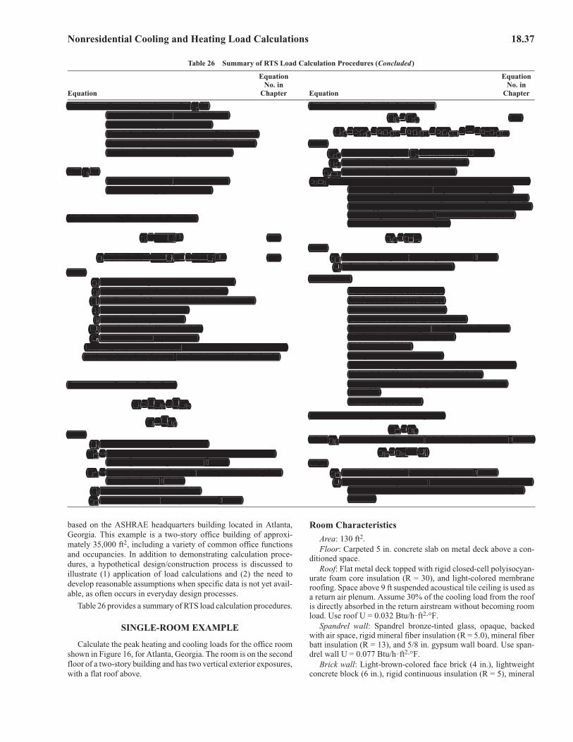
Nonresidential Cooling and Heating Load Calculations 18.37
Table 26 Summary of RTS Load Calculation Procedures (Concluded)
Equation
Equation No. in
Chapter Equation
Equation No. in
Chapter
For other appliances and equipment, find qs forUnhooded cooking appliances: Table 5AOther kitchen equipment: Table 5EHospital and laboratory equipment: Tables 6 and 7Computers, printers, scanners, etc.: Tables 8 and 9Miscellaneous office equipment: Table 10
Find ql forUnhooded cooking appliances: Table 5AOther kitchen equipment: Table 5E
Ventilation and Infiltration Air Heat Gain
qs = 1.10Qst (10)
ql = 60 × 0.075 × 1076QsW = 4840QsW (11)
whereqs = sensible heat gain due to infiltration, Btu/hql = latent heat gain due to infiltration, Btu/h
Qs = infiltration airflow at standard air conditions, cfmto = outdoor air temperature, °Fti = indoor air temperature, °F
Wo = outdoor air humidity ratio, lb/lbWi = indoor air humidity ratio, lb/lb
1.10 = air sensible heat factor at standard air conditions, Btu/h·cfm4840 = air latent heat factor at standard air conditions, Btu/h·cfm
Instantaneous Room Cooling Load
Qs = �Qi,r + �Qi,c
Ql = �qi,l
whereQs = room sensible cooling load, Btu/h
Qi,r = radiant portion of sensible cooling load for current hour, resulting from heat gain element i, Btu/h
Qi,c = convective portion of sensible cooling load, resulting from heat gain element i, Btu/h
Ql = room latent cooling load, Btu/hqi,l = latent heat gain for heat gain element i, Btu/h
Radiant Portion of Sensible Cooling Load
(34)Qi,r = Qr,�
Qr,� = r0qr,� + r1qr,�–1 + r2qr,�–2 + r3qr,�–3 + … + r23qr,�–23
whereQr,� = radiant cooling load Qr for current hour �, Btu/hqr,� = radiant heat gain for current hour, Btu/h
qr,��n = radiant heat gain n hours ago, Btu/hr0, r1, etc. = radiant time factors; see Table 19 for radiant time factors for
nonsolar heat gains: wall, roof, partition, ceiling, floor, fenestration transmission heat gains, and occupant, lighting, motor, appliance heat gain. Also used for fenestration diffuse solar heat gain; see Table 20 for radiant time factors for fenestration beam solar heat gain.
qr,� = qi,sFr
whereqi,s = sensible heat gain from heat gain element i, Btu/hFr = fraction of heat gain that is radiant.
Data Sources:
Wall transmission: see Table 14Roof transmission: see Table 14Floor transmission: see Table 14Fenestration transmission: see Table 14Fenestration solar heat gain: see Table 14, Chapter 18 and Tables 13A to 13G, Chapter 15Lighting: see Table 3Occupants: see Tables 1 and 14Hooded cooking appliances: see Tables 5B, 5C, and 5DUnhooded cooking appliances: see Table 5AOther appliances and equipment: see Tables 5E, 8, 9, 10, and 14Infiltration: see Table 14
Convective Portion of Sensible Cooling Load
Qi,c = qi,c
where qi,c is convective portion of heat gain from heat gain element i, Btu/h.
qi,c = qi,s(1 – Fr)
whereqi,s = sensible heat gain from heat gain element i, Btu/hFr = fraction of heat gain that is radiant; see row for radiant portion
for sources of radiant fraction data for individual heat gain elements
based on the ASHRAE headquarters building located in Atlanta,Georgia. This example is a two-story office building of approxi-mately 35,000 ft2, including a variety of common office functionsand occupancies. In addition to demonstrating calculation proce-dures, a hypothetical design/construction process is discussed toillustrate (1) application of load calculations and (2) the need todevelop reasonable assumptions when specific data is not yet avail-able, as often occurs in everyday design processes.
Table 26 provides a summary of RTS load calculation procedures.
SINGLE-ROOM EXAMPLE
Calculate the peak heating and cooling loads for the office roomshown in Figure 16, for Atlanta, Georgia. The room is on the secondfloor of a two-story building and has two vertical exterior exposures,with a flat roof above.
Room Characteristics
Area: 130 ft2. Floor: Carpeted 5 in. concrete slab on metal deck above a con-
ditioned space.Roof: Flat metal deck topped with rigid closed-cell polyisocyan-
urate foam core insulation (R = 30), and light-colored membraneroofing. Space above 9 ft suspended acoustical tile ceiling is used asa return air plenum. Assume 30% of the cooling load from the roofis directly absorbed in the return airstream without becoming roomload. Use roof U = 0.032 Btu/h·ft2·°F.
Spandrel wall: Spandrel bronze-tinted glass, opaque, backedwith air space, rigid mineral fiber insulation (R = 5.0), mineral fiberbatt insulation (R = 13), and 5/8 in. gypsum wall board. Use span-drel wall U = 0.077 Btu/h·ft2·°F.
Brick wall: Light-brown-colored face brick (4 in.), lightweightconcrete block (6 in.), rigid continuous insulation (R = 5), mineral
For other appliances and equipment, find qs for Radiant Portion of Sensible Cooling LoadUnhooded cooking appliances: Table 5A Qi, = Qr, (34),r r r,�Other kitchen equipment: Table 5E
… Qr,rr = r0qr, + r1qr, + r2qr, + r3qr, + + r23qr,Hospital and laboratory equipment: Tables 6 and 7 r,� r,� r,�––1 r,�––2 r,�––3 r,�––23
Computers, printers, scanners, etc.: Tables 8 and 9 whereMiscellaneous office equipment: Table 10 Qr, = radiant cooling load Qr r for current hour �, Btu/hr,�
qr, = radiant heat gain for current hour, Btu/hr,�Find ql for qr, = radiant heat gain n hours ago, Btu/hr,��n
Unhooded cooking appliances: Table 5A r0, r1, etc. = radiant time factors; see Table 19 for radiant time factors for nonsolar heat gains: wall, roof, partition, ceiling, floor,Other kitchen equipment: Table 5Efenestration transmission heat gains, and occupant, lighting, motor, appliance heat gain. Also used for fenestration diffuse solar heat gain; see Table 20 for radiant time factors for Ventilation and Infiltration Air Heat Gainfenestration beam solar heat gain.
qs = 1.10QsQst (10) qr, = qi,sFss rFFr,�
whereql l = 60 × 0.075 × 1076QsQsW W = W 4840QsQsW (11) qi, = sensible heat gain from heat gain element i, Btu/h,s
FrFF = fraction of heat gain that is radiant.where
Data Sources:qs = sensible heat gain due to infiltration, Btu/hql = latent heat gain due to infiltration, Btu/h Wall transmission: see Table 14
QsQ = infiltration airflow at standard air conditions, cfm Roof transmission: see Table 14to = outdoor air temperature, °F Floor transmission: see Table 14ti = indoor air temperature, °F Fenestration transmission: see Table 14
WoWW = outdoor air humidity ratio, lb/lb Fenestration solar heat gain: see Table 14, Chapter 18and Tables 13A to 13G, Chapter 15WiWW = indoor air humidity ratio, lb/lbLighting: see Table 31.10 = air sensible heat factor at standard air conditions, Btu/h·cfmOccupants: see Tables 1 and 144840 = air latent heat factor at standard air conditions, Btu/h·cfmHooded cooking appliances: see Tables 5B, 5C, and 5DUnhooded cooking appliances: see Table 5AOther appliances and equipment: see Tables 5E, 8, 9, Instantaneous Room Cooling Load10, and 14
� � Infiltration: see Table 14Qs = �Qi, + �Qi,,r r ,c
Convective Portion of Sensible Cooling Load�Ql l = �qi,,lQi, = qi,,c ,cwhere
where qi, is convective portion of heat gain from heat gain element i, Btu/h.,c QsQ = room sensible cooling load, Btu/hqi, = qi,s((1 – FrFF )Qi, = radiant portion of sensible cooling load for current hour, ,c ,r
resulting from heat gain element i, Btu/h whereQi, = convective portion of sensible cooling load, resulting from qi, = sensible heat gain from heat gain element i, Btu/h,c ,s
heat gain element i, Btu/h FrFF = fraction of heat gain that is radiant; see row for radiant portionQl = room latent cooling load, Btu/h for sources of radiant fraction data for individual heat gain
elementsqi, = latent heat gain for heat gain element i, Btu/h,l
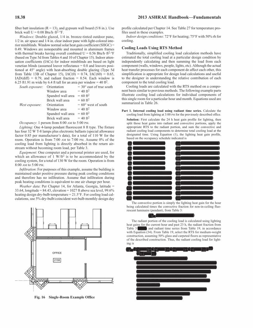
18.38 2013 ASHRAE Handbook—Fundamentals
fiber batt insulation (R = 13), and gypsum wall board (5/8 in.). Usebrick wall U = 0.08 Btu/h·ft2·°F.
Windows: Double glazed, 1/4 in. bronze-tinted outdoor pane,1/2 in. air space and 1/4 in. clear indoor pane with light-colored inte-rior miniblinds. Window normal solar heat gain coefficient (SHGC) =0.49. Windows are nonoperable and mounted in aluminum frameswith thermal breaks having overall combined U = 0.56 Btu/h·ft2·°F(based on Type 5d from Tables 4 and 10 of Chapter 15). Indoor atten-uation coefficients (IACs) for indoor miniblinds are based on lightvenetian blinds (assumed louver reflectance = 0.8 and louvers posi-tioned at 45° angle) with heat-absorbing double glazing (Type 5dfrom Table 13B of Chapter 15), IAC(0) = 0.74, IAC(60) = 0.65,IAD(diff) = 0.79, and radiant fraction = 0.54. Each window is6.25 ft1.91 m wide by 6.4 ft tall for an area per window = 40 ft2.
South exposure: Orientation = 30° east of true southWindow area = 40 ft2
Spandrel wall area = 60 ft2
Brick wall area = 60 ft2
West exposure: Orientation = 60° west of southWindow area = 40 ft2
Spandrel wall area = 60 ft2
Brick wall area = 40 ft2
Occupancy: 1 person from 8:00 AM to 5:00 PM.Lighting: One 4-lamp pendant fluorescent 8 ft type. The fixture
has four 32 W T-8 lamps plus electronic ballasts (special allowancefactor 0.85 per manufacturer’s data), for a total of 110 W for theroom. Operation is from 7:00 AM to 7:00 PM. Assume 0% of thecooling load from lighting is directly absorbed in the return air-stream without becoming room load, per Table 3.
Equipment: One computer and a personal printer are used, forwhich an allowance of 1 W/ft2 is to be accommodated by thecooling system, for a total of 130 W for the room. Operation is from8:00 AM to 5:00 PM.
Infiltration: For purposes of this example, assume the building ismaintained under positive pressure during peak cooling conditionsand therefore has no infiltration. Assume that infiltration duringpeak heating conditions is equivalent to one air change per hour.
Weather data: Per Chapter 14, for Atlanta, Georgia, latitude =33.64, longitude = 84.43, elevation = 1027 ft above sea level, 99.6%heating design dry-bulb temperature = 21.5°F. For cooling load cal-culations, use 5% dry-bulb/coincident wet-bulb monthly design day
profile calculated per Chapter 14. See Table 27 for temperature pro-files used in these examples.
Indoor design conditions: 72°F for heating; 75°F with 50% rh forcooling.
Cooling Loads Using RTS MethodTraditionally, simplified cooling load calculation methods have
estimated the total cooling load at a particular design condition byindependently calculating and then summing the load from eachcomponent (walls, windows, people, lights, etc). Although the actualheat transfer processes for each component do affect each other, thissimplification is appropriate for design load calculations and usefulto the designer in understanding the relative contribution of eachcomponent to the total cooling load.
Cooling loads are calculated with the RTS method on a compo-nent basis similar to previous methods. The following example partsillustrate cooling load calculations for individual components ofthis single room for a particular hour and month. Equations used aresummarized in Table 26.
Part 1. Internal cooling load using radiant time series. Calculate thecooling load from lighting at 3:00 PM for the previously described office.
Solution: First calculate the 24 h heat gain profile for lighting, thensplit those heat gains into radiant and convective portions, apply theappropriate RTS to the radiant portion, and sum the convective andradiant cooling load components to determine total cooling load at thedesignated time. Using Equation (1), the lighting heat gain profile,based on the occupancy schedule indicated is
q1 = (110 W)3.41(0%) = 0 q13 = (110 W)3.41(100%) = 375
q2 = (110 W)3.41(0%) = 0 q14 = (110 W)3.41(100%) = 375
q3 = (110 W)3.41(0%) = 0 q15 = (110 W)3.41(100%) = 375
q4 = (110 W)3.41(0%) = 0 q16 = (110 W)3.41(100%) = 375
q5 = (110 W)3.41(0%) = 0 q17 = (110 W)3.41(100%) = 375
q6 = (110 W)3.41(0%) = 0 q18 = (110 W)3.41(100%) = 375
q7 = (110 W)3.41(100%) = 375 q19 = (110 W)3.41(0%) = 0
q8 = (110 W)3.41(100%) = 375 q20 = (110 W)3.41(0%) = 0
q9 = (110 W)3.41(100%) = 375 q21 = (110 W)3.41(0%) = 0
q10 = (110 W)3.41(100%) = 375 q22 = (110 W)3.41(0%) = 0
q11 = (110 W)3.41(100%) = 375 q23 = (110 W)3.41(0%) = 0
q12 = (110 W)3.41(100%) = 375 q24 = (110 W)3.41(0%) = 0
The convective portion is simply the lighting heat gain for the hourbeing calculated times the convective fraction for non-in-ceiling fluo-rescent luminaire (pendant), from Table 3:
Qc,15 = (375)(43%) = 161.3 Btu/h
The radiant portion of the cooling load is calculated using lightingheat gains for the current hour and past 23 h, the radiant fraction fromTable 3 (57%), and radiant time series from Table 19, in accordancewith Equation (34). From Table 19, select the RTS for medium-weightconstruction, assuming 50% glass and carpeted floors as representativeof the described construction. Thus, the radiant cooling load for light-ing is
Qr,15 = r0(0.48)q15 + r1(0.48)q14 + r2(0.48)q13 + r3(0.48)q12 + … + r23(0.48)q16
= (0.49)(0.57)(375) + (0.17)(0.57)(375)+ (0.09)(0.57)(375) + (0.05)(0.57)(375) + (0.03)(0.57)(375)+ (0.02)(0.57)(375) + (0.02)(0.57)(375) + (0.01)(0.57)(375)+ (0.01)(0.57)(375) + (0.01)(0.57) (0) + (0.01)(0.57)(0)+ (0.01)(0.57)(0) + (0.01)(0.57)(0) + (0.01)(0.57)(0)+ (0.01)(0.5748)(0) + (0.01)(0.57)(0) + (0.01)(0.57)(0)+ (0.01)(0.57)(0)+ (0.01)(0.57)(0) + (0.01)(0.57)(0) + (0.00)(0.57)(0)+ (0.00)(0.57)(375) + (0.00)(0.57)(375)+ (0.00)(0.57)(375) = 190.3 Btu/hFig. 16 Single-Room Example Office
q1 = (110 W)3.41(0%) = 0 q13 = (110 W)3.41(100%) = 375
q2 = (110 W)3.41(0%) = 0 q14 = (110 W)3.41(100%) = 375
q3 = (110 W)3.41(0%) = 0 q15 = (110 W)3.41(100%) = 375
q4 = (110 W)3.41(0%) = 0 q16 = (110 W)3.41(100%) = 375
q5 = (110 W)3.41(0%) = 0 q17 = (110 W)3.41(100%) = 375
q6 = (110 W)3.41(0%) = 0 q18 = (110 W)3.41(100%) = 375
q7 = (110 W)3.41(100%) = 375 q19 = (110 W)3.41(0%) = 0
q8 = (110 W)3.41(100%) = 375 q20 = (110 W)3.41(0%) = 0
q9 = (110 W)3.41(100%) = 375 q21 = (110 W)3.41(0%) = 0
q10 = (110 W)3.41(100%) = 375 q22 = (110 W)3.41(0%) = 0
q11 = (110 W)3.41(100%) = 375 q23 = (110 W)3.41(0%) = 0
q12 = (110 W)3.41(100%) = 375 q24 = (110 W)3.41(0%) = 0
Qc, = (375)(43%) = 161.3 Btu/h,15
(57%),
…Qr, = r0((0.48))q15 + r1((0.48))q14 + r2((0.48))q13 + r3((0.48))q12 + r,15 + r23((0.48))q16
= (0.49)(0.57)(375) + (0.17)(0.57)(375)+ (0.09)(0.57)(375) + (0.05)(0.57)(375) + (0.03)(0.57)(375)+ (0.02)(0.57)(375) + (0.02)(0.57)(375) + (0.01)(0.57)(375)+ (0.01)(0.57)(375) + (0.01)(0.57) (0) + (0.01)(0.57)(0)+ (0.01)(0.57)(0) + (0.01)(0.57)(0) + (0.01)(0.57)(0)+ (0.01)(0.5748)(0) + (0.01)(0.57)(0) + (0.01)(0.57)(0)+ (0.01)(0.57)(0)+ (0.01)(0.57)(0) + (0.01)(0.57)(0) + (0.00)(0.57)(0)+ (0.00)(0.57)(375) + (0.00)(0.57)(375)+ (0.00)(0.57)(375) = 190.3 Btu/h
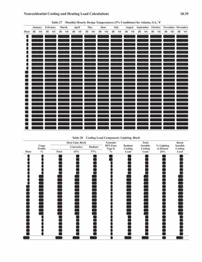
Nonresidential Cooling and Heating Load Calculations 18.39
Table 27 Monthly/Hourly Design Temperatures (5% Conditions) for Atlanta, GA, °F
January February March April May June July August September October November December
Hour db wb db wb db wb db wb db wb db wb db wb db wb db wb db wb db wb db wb
1 44.8 44.0 47.4 45.7 53.1 48.7 59.4 54.3 66.4 61.9 72.2 66.7 73.9 68.9 73.8 69.3 69.5 64.9 60.1 56.8 52.5 50.8 46.4 46.3
2 44.0 43.4 46.6 45.1 52.1 48.2 58.5 53.9 65.6 61.6 71.4 66.4 73.0 68.7 73.1 69.1 68.7 64.6 59.3 56.4 51.7 50.3 45.6 45.6
3 43.4 43.0 46.0 44.8 51.5 47.9 57.8 53.6 65.0 61.4 70.8 66.2 72.4 68.5 72.5 68.9 68.2 64.4 58.7 56.2 51.0 50.0 45.0 45.0
4 42.8 42.6 45.3 44.4 50.8 47.5 57.2 53.3 64.4 61.2 70.2 66.0 71.8 68.3 71.9 68.7 67.6 64.2 58.1 55.9 50.4 49.6 44.4 44.4
5 42.4 42.3 44.9 44.1 50.3 47.3 56.7 53.1 64.0 61.0 69.8 65.9 71.4 68.2 71.5 68.6 67.2 64.1 57.7 55.7 50.0 49.4 44.0 44.0
6 42.8 42.6 45.3 44.4 50.8 47.5 57.2 53.3 64.4 61.2 70.2 66.0 71.8 68.3 71.9 68.7 67.6 64.2 58.1 55.9 50.4 49.6 44.4 44.4
7 44.2 43.6 46.8 45.3 52.4 48.3 58.8 54.0 65.8 61.7 71.6 66.5 73.2 68.8 73.2 69.1 68.9 64.7 59.5 56.5 51.9 50.4 45.8 45.8
8 47.7 46.0 50.4 47.5 56.3 50.3 62.6 55.6 69.3 63.0 75.1 67.6 76.7 69.8 76.5 70.2 72.2 65.9 63.0 58.1 55.4 52.4 49.1 48.2
9 51.6 48.7 54.4 50.0 60.7 52.4 67.0 57.5 73.1 64.5 78.9 68.8 80.6 71.0 80.2 71.3 75.8 67.2 66.8 59.8 59.4 54.6 52.9 50.9
10 55.0 51.1 57.9 52.2 64.6 54.4 70.8 59.1 76.6 65.8 82.3 69.9 84.1 72.0 83.5 72.3 79.0 68.3 70.3 61.3 62.9 56.6 56.3 53.2
11 58.1 53.2 61.1 54.1 68.0 56.1 74.3 60.6 79.6 66.9 85.4 70.9 87.2 73.0 86.4 73.2 81.9 69.3 73.3 62.7 66.0 58.3 59.2 55.3
12 60.1 54.7 63.2 55.4 70.3 57.2 76.5 61.5 81.7 67.7 87.4 71.6 89.2 73.6 88.4 73.8 83.8 70.0 75.4 63.6 68.1 59.5 61.2 56.7
13 61.8 55.8 64.9 56.5 72.2 58.1 78.4 62.3 83.3 68.3 89.0 72.1 90.9 74.1 89.9 74.3 85.3 70.6 77.0 64.3 69.8 60.4 62.8 57.8
14 62.8 56.5 65.9 57.1 73.3 58.7 79.5 62.8 84.3 68.7 90.0 72.4 91.9 74.4 90.9 74.6 86.3 70.9 78.0 64.8 70.8 61.0 63.8 58.5
15 62.8 56.5 65.9 57.1 73.3 58.7 79.5 62.8 84.3 68.7 90.0 72.4 91.9 74.4 90.9 74.6 86.3 70.9 78.0 64.8 70.8 61.0 63.8 58.5
16 61.6 55.6 64.6 56.3 71.9 58.0 78.1 62.2 83.1 68.2 88.8 72.0 90.7 74.0 89.7 74.2 85.2 70.5 76.8 64.3 69.6 60.3 62.6 57.7
17 59.9 54.5 63.0 55.3 70.1 57.1 76.3 61.4 81.5 67.6 87.2 71.5 89.0 73.5 88.2 73.8 83.6 69.9 75.2 63.5 67.9 59.4 61.0 56.6
18 57.9 53.1 60.9 54.0 67.8 56.0 74.0 60.5 79.4 66.9 85.2 70.8 87.0 72.9 86.2 73.2 81.7 69.3 73.1 62.6 65.8 58.2 59.0 55.2
19 54.8 51.0 57.7 52.0 64.3 54.3 70.6 59.0 76.4 65.7 82.1 69.9 83.9 72.0 83.3 72.3 78.9 68.2 70.1 61.3 62.7 56.5 56.1 53.1
20 52.6 49.4 55.4 50.6 61.8 53.0 68.1 58.0 74.2 64.9 79.9 69.2 81.7 71.3 81.2 71.6 76.8 67.5 67.9 60.3 60.4 55.2 53.9 51.6
21 50.8 48.1 53.5 49.4 59.7 52.0 66.0 57.1 72.3 64.2 78.1 68.6 79.8 70.7 79.5 71.1 75.0 66.9 66.0 59.4 58.5 54.2 52.1 50.3
22 48.9 46.8 51.6 48.3 57.7 50.9 64.0 56.2 70.5 63.5 76.3 68.0 78.0 70.2 77.7 70.5 73.3 66.3 64.2 58.6 56.7 53.1 50.3 49.0
23 47.5 45.9 50.2 47.4 56.1 50.2 62.4 55.5 69.1 62.9 74.9 67.5 76.5 69.8 76.4 70.1 72.0 65.8 62.8 58.0 55.2 52.3 49.0 48.1
24 46.1 44.9 48.7 46.4 54.4 49.4 60.8 54.8 67.7 62.4 73.4 67.1 75.1 69.3 75.0 69.7 70.6 65.3 61.4 57.3 53.7 51.5 47.6 47.1
Table 28 Cooling Load Component: Lighting, Btu/h
Hour
UsageProfile,
%
Heat Gain, Btu/h NonsolarRTS Zone
Type 8,%
Radiant Cooling
Load
TotalSensible Cooling
Load
% Lightingto Return
26%
RoomSensible Cooling
Load
Convective Radiant
Total 43% 57%
1 0 — — — 49 26 26 — 262 0 — — — 17 26 26 — 263 0 — — — 9 24 24 — 244 0 — — — 5 21 21 — 215 0 — — — 3 19 19 — 196 0 — — — 2 17 17 — 177 100 375 161 214 2 120 281 — 2818 100 375 161 214 1 154 315 — 3159 100 375 161 214 1 171 332 — 332
10 100 375 161 214 1 180 341 — 34111 100 375 161 214 1 184 345 — 34512 100 375 161 214 1 186 347 — 34713 100 375 161 214 1 188 349 — 34914 100 375 161 214 1 188 349 — 34915 100 375 161 214 1 190 352 — 35216 100 375 161 214 1 192 354 — 35417 100 375 161 214 1 195 356 — 35618 100 375 161 214 1 197 358 — 35819 0 — — — 1 94 94 — 9420 0 — — — 1 60 60 — 6021 0 — — — 0 43 43 — 4322 0 — — — 0 34 34 — 3423 0 — — — 0 30 30 — 3024 0 — — — 0 28 28 — 28
Total 4,501 1,936 2,566 1 2,566 4,501 — 4,501
1 44.8 44.0 47.4 45.7 53.1 48.7 59.4 54.3 66.4 61.9 72.2 66.7 73.9 68.9 73.8 69.3 69.5 64.9 60.1 56.8 52.5 50.8 46.4 46.3
2 44.0 43.4 46.6 45.1 52.1 48.2 58.5 53.9 65.6 61.6 71.4 66.4 73.0 68.7 73.1 69.1 68.7 64.6 59.3 56.4 51.7 50.3 45.6 45.6
3 43.4 43.0 46.0 44.8 51.5 47.9 57.8 53.6 65.0 61.4 70.8 66.2 72.4 68.5 72.5 68.9 68.2 64.4 58.7 56.2 51.0 50.0 45.0 45.0
4 42.8 42.6 45.3 44.4 50.8 47.5 57.2 53.3 64.4 61.2 70.2 66.0 71.8 68.3 71.9 68.7 67.6 64.2 58.1 55.9 50.4 49.6 44.4 44.4
5 42.4 42.3 44.9 44.1 50.3 47.3 56.7 53.1 64.0 61.0 69.8 65.9 71.4 68.2 71.5 68.6 67.2 64.1 57.7 55.7 50.0 49.4 44.0 44.0
6 42.8 42.6 45.3 44.4 50.8 47.5 57.2 53.3 64.4 61.2 70.2 66.0 71.8 68.3 71.9 68.7 67.6 64.2 58.1 55.9 50.4 49.6 44.4 44.4
7 44.2 43.6 46.8 45.3 52.4 48.3 58.8 54.0 65.8 61.7 71.6 66.5 73.2 68.8 73.2 69.1 68.9 64.7 59.5 56.5 51.9 50.4 45.8 45.8
8 47.7 46.0 50.4 47.5 56.3 50.3 62.6 55.6 69.3 63.0 75.1 67.6 76.7 69.8 76.5 70.2 72.2 65.9 63.0 58.1 55.4 52.4 49.1 48.2
9 51.6 48.7 54.4 50.0 60.7 52.4 67.0 57.5 73.1 64.5 78.9 68.8 80.6 71.0 80.2 71.3 75.8 67.2 66.8 59.8 59.4 54.6 52.9 50.9
10 55.0 51.1 57.9 52.2 64.6 54.4 70.8 59.1 76.6 65.8 82.3 69.9 84.1 72.0 83.5 72.3 79.0 68.3 70.3 61.3 62.9 56.6 56.3 53.2
11 58.1 53.2 61.1 54.1 68.0 56.1 74.3 60.6 79.6 66.9 85.4 70.9 87.2 73.0 86.4 73.2 81.9 69.3 73.3 62.7 66.0 58.3 59.2 55.3
12 60.1 54.7 63.2 55.4 70.3 57.2 76.5 61.5 81.7 67.7 87.4 71.6 89.2 73.6 88.4 73.8 83.8 70.0 75.4 63.6 68.1 59.5 61.2 56.7
13 61.8 55.8 64.9 56.5 72.2 58.1 78.4 62.3 83.3 68.3 89.0 72.1 90.9 74.1 89.9 74.3 85.3 70.6 77.0 64.3 69.8 60.4 62.8 57.8
14 62.8 56.5 65.9 57.1 73.3 58.7 79.5 62.8 84.3 68.7 90.0 72.4 91.9 74.4 90.9 74.6 86.3 70.9 78.0 64.8 70.8 61.0 63.8 58.5
15 62.8 56.5 65.9 57.1 73.3 58.7 79.5 62.8 84.3 68.7 90.0 72.4 91.9 74.4 90.9 74.6 86.3 70.9 78.0 64.8 70.8 61.0 63.8 58.5
16 61.6 55.6 64.6 56.3 71.9 58.0 78.1 62.2 83.1 68.2 88.8 72.0 90.7 74.0 89.7 74.2 85.2 70.5 76.8 64.3 69.6 60.3 62.6 57.7
17 59.9 54.5 63.0 55.3 70.1 57.1 76.3 61.4 81.5 67.6 87.2 71.5 89.0 73.5 88.2 73.8 83.6 69.9 75.2 63.5 67.9 59.4 61.0 56.6
18 57.9 53.1 60.9 54.0 67.8 56.0 74.0 60.5 79.4 66.9 85.2 70.8 87.0 72.9 86.2 73.2 81.7 69.3 73.1 62.6 65.8 58.2 59.0 55.2
19 54.8 51.0 57.7 52.0 64.3 54.3 70.6 59.0 76.4 65.7 82.1 69.9 83.9 72.0 83.3 72.3 78.9 68.2 70.1 61.3 62.7 56.5 56.1 53.1
20 52.6 49.4 55.4 50.6 61.8 53.0 68.1 58.0 74.2 64.9 79.9 69.2 81.7 71.3 81.2 71.6 76.8 67.5 67.9 60.3 60.4 55.2 53.9 51.6
21 50.8 48.1 53.5 49.4 59.7 52.0 66.0 57.1 72.3 64.2 78.1 68.6 79.8 70.7 79.5 71.1 75.0 66.9 66.0 59.4 58.5 54.2 52.1 50.3
22 48.9 46.8 51.6 48.3 57.7 50.9 64.0 56.2 70.5 63.5 76.3 68.0 78.0 70.2 77.7 70.5 73.3 66.3 64.2 58.6 56.7 53.1 50.3 49.0
23 47.5 45.9 50.2 47.4 56.1 50.2 62.4 55.5 69.1 62.9 74.9 67.5 76.5 69.8 76.4 70.1 72.0 65.8 62.8 58.0 55.2 52.3 49.0 48.1
24 46.1 44.9 48.7 46.4 54.4 49.4 60.8 54.8 67.7 62.4 73.4 67.1 75.1 69.3 75.0 69.7 70.6 65.3 61.4 57.3 53.7 51.5 47.6 47.1
1 0 — — — 49 26 26 — 262 0 — — — 17 26 26 — 263 0 — — — 9 24 24 — 244 0 — — — 5 21 21 — 215 0 — — — 3 19 19 — 196 0 — — — 2 17 17 — 177 100 375 161 214 2 120 281 — 2818 100 375 161 214 1 154 315 — 3159 100 375 161 214 1 171 332 — 332
10 100 375 161 214 1 180 341 — 34111 100 375 161 214 1 184 345 — 34512 100 375 161 214 1 186 347 — 34713 100 375 161 214 1 188 349 — 34914 100 375 161 214 1 188 349 — 34915 100 375 161 214 1 190 352 — 35216 100 375 161 214 1 192 354 — 35417 100 375 161 214 1 195 356 — 35618 100 375 161 214 1 197 358 — 35819 0 — — — 1 94 94 — 9420 0 — — — 1 60 60 — 6021 0 — — — 0 43 43 — 4322 0 — — — 0 34 34 — 3423 0 — — — 0 30 30 — 3024 0 — — — 0 28 28 — 28
Total 4,501 1,936 2,566 1 2,566 4,501 — 4,501

18.40 2013 ASHRAE Handbook—Fundamentals
The total lighting cooling load at the designated hour is thusQlight = Qc,15 + Qr,15 = 161.3 + 190.3 = 351.6 Btu/h
See Table 28 for the office’s lighting usage, heat gain, and coolingload profiles.
Part 2. Wall cooling load using sol-air temperature, conduction timeseries and radiant time series. Calculate the cooling load contributionfrom the spandrel wall section facing 60° west of south at 3:00 PM localstandard time in July for the previously described office.
Solution: Determine the wall cooling load by calculating (1) sol-airtemperatures at the exterior surface, (2) heat input based on sol-air tem-perature, (3) delayed heat gain through the mass of the wall to the inte-rior surface using conduction time series, and (4) delayed space coolingload from heat gain using radiant time series.
First, calculate the sol-air temperature at 3:00 PM local standardtime (LST) (4:00 PM daylight saving time) on July 21 for a vertical,dark-colored wall surface, facing 60° west of south, located in Atlanta,Georgia (latitude = 33.64, longitude = 84.43), solar taub = 0.440 andtaud = 2.202 from monthly Atlanta weather data for July (Table 1 inChapter 14). From Table 26, the calculated outdoor design temperaturefor that month and time is 92°F. The ground reflectivity is assumed�g = 0.2.
Sol-air temperature is calculated using Equation (30). For the dark-colored wall, �/ho = 0.30, and for vertical surfaces, �R/ho = 0. Thesolar irradiance Et on the wall must be determined using the equationsin Chapter 14:
Solar Angles:
= southwest orientation = +60°� = surface tilt from horizontal (where horizontal = 0°) = 90° for
vertical wall surface3:00 PM LST = hour 15
Calculate solar altitude, solar azimuth, surface solar azimuth, andincident angle as follows:
From Table 2 in Chapter 14, solar position data and constants forJuly 21 are
ET = –6.4 min� = 20.4°
Eo = 419.8 Btu/h·ft2
Local standard meridian (LSM) for Eastern Time Zone = 75°.
Apparent solar time AST
AST = LST + ET/60 + (LSM – LON)/15 = 15 + (–6.4/60) + [(75 – 84.43)/15]
= 14.2647
Hour angle H, degrees
H = 15(AST – 12) = 15(14.2647 – 12) = 33.97°
Solar altitude !sin ! = cos L cos � cos H + sin L sin �
= cos (33.64) cos (20.4) cos (33.97) + sin (33.64) sin (20.4)= 0.841
� ! = sin–1(0.841) = 57.2°
Solar azimuth "cos " = (sin ! sin L – sin �)/(cos ! cos L)
= [(sin (57.2)sin (33.64) – sin (20.4)]/[cos (57.2) cos (33.64)]= 0.258
" = cos–1(0.253) = 75.05°
Surface-solar azimuth ## = " – = 75.05 – 60 = 15.05°
Incident angle �cos � = cos ! cos g sin � + sin ! cos �
= cos (57.2) cos (15.05) sin (90) + sin (57.2) cos (90)= 0.523
� = cos–1(0.523) = 58.45°
Beam normal irradiance Eb
Eb = Eo exp(–�bmab)m = relative air mass
= 1/[sin! +0.50572(6.07995 + !)–1.6364], ! expressed in degrees= 1.18905
ab = beam air mass exponent= 1.454 – 0.406�b – 0.268�d + 0.021�b�d= 0.7055705
Eb = 419.8 exp[–0.556(1.89050.7055705)]= 255.3 Btu/h·ft2
Surface beam irradiance Et,b
Et,b = Eb cos�= (255.3) cos (58.5)
= 133.6 Btu/h·ft2
Ratio Y of sky diffuse radiation on vertical surface to sky diffuse radia-tion on horizontal surface
Y = 0.55 + 0.437 cos � + 0.313 cos2�= 0.55 + 0.437 cos (58.45) + 0.313 cos2(58.45)= 0.8644
Diffuse irradiance Ed – Horizontal surfaces
Ed = Eo exp(–�d mad)ad = diffuse air mass exponent
= 0.507 + 0.205�b – 0.080 �d – 0.190 �b�d= 0.2369528
Ed = Eo exp(–�d mad)= 419.8 exp[–2.202(1.89050.2369528)]= 42.3 Btu/h·ft2
Diffuse irradiance Ed – Vertical surfaces
Et,d = EdY= (42.3)(0.864)= 36.6 Btu/h·ft2
Ground reflected irradiance Et,r
Et,r = (Eb sin! + Ed)�g(l – cos ��$%= [%&&'( sin (57.2) + 42.3](0.2)[1 – cos (90)]/2= 25.7 Btu/h·ft2
Total surface irradiance Et
Et = ED + Ed + Er = 133.6 + 36.6 + 25.7 = 195.9 Btu/h·ft2
Sol-air temperature [from Equation (30)]:
Te = to + �Et /ho – �R/ho = 91.9 + (0.30)(195.9) – 0 = 150.7°F
This procedure is used to calculate the sol-air temperatures for eachhour on each surface. Because of the tedious solar angle and intensitycalculations, using a simple computer spreadsheet or other computersoftware can reduce the effort involved. A spreadsheet was used to cal-culate a 24 h sol-air temperature profile for the data of this example.See Table 29A for the solar angle and intensity calculations and Table29B for the sol-air temperatures for this wall surface and orientation.
Conductive heat gain is calculated using Equations (31) and (32).First, calculate the 24 h heat input profile using Equation (31) and thesol-air temperatures for a southwest-facing wall with dark exteriorcolor:
qi,1 = (0.077)(60)(73.9 – 75) = –5 Btu/hqi,2 = (0.077)(60)(73 – 75) = –9qi,3 = (0.077)(60)(72.4 – 75) = –12qi,4 = (0.077)(60)(71.8 – 75) = –15qi,5 = (0.077)(60)(71.4 – 75) = –17qi,6 = (0.077)(60)(72.8 – 75) = –10qi,7 = (0.077)(60)(77.4 – 75) = 11qi,8 = (0.077)(60)(84.1 – 75) = 42qi,9 = (0.077)(60)(90.8 – 75) = 73
qi,10 = (0.077)(60)(96.7 – 75) = 100qi,11 = (0.077)(60)(101.5 – 75) = 122qi,12 = (0.077)(60)(105.5 – 75) = 141qi,13 = (0.077)(60)(122.4 – 75) = 219
(1) sol-airtemperatures at the exterior surface, (2) heat input based on sol-air tem-perature, (3) delayed heat gain through the mass of the wall to the inte-rior surface using conduction time series, and (4) delayed space coolingload from heat gain using radiant time series.
First, calculate the sol-air temperature at 3:00 local standardPM time (LST) (4:00 daylight saving time) on July 21 for a vertical,PM dark-colored wall surface, facing 60° west of south, located in Atlanta,Georgia (latitude = 33.64, longitude = 84.43), solar taub = 0.440 andtaud = 2.202 from monthly Atlanta weather data for July (Table 1 inChapter 14). From Table 26, the calculated outdoor design temperaturefor that month and time is 92°F. The ground reflectivity is assumed� = 0.2.�g�
Sol-air temperature is calculated using Equation (30). For the dark-colored wall, �//ho = 0.30, and for vertical surfaces, �R//ho = 0. Thesolar irradiance Et t
oon the wall must be determined using the equations
in Chapter 14:
Solar Angles:
= southwest orientation = +60°� = surface tilt from horizontal (where horizontal = 0°) = 90° for
vertical wall surface3:00 LST = hour 15PM
Calculate solar altitude, solar azimuth, surface solar azimuth, andincident angle as follows:
From Table 2 in Chapter 14, solar position data and constants forJuly 21 are
ET = –6.4 min� = 20.4°
ft2EoE = 419.8 Btu/h·f
Local standard meridian (LSM) for Eastern Time Zone = 75°.
Apparent solar time AST
AST = LST + ET/60 + (LSM – LON)/15= 15 + (–6.4/60) + [(75 – 84.43)/15]
= 14.2647
Hour angle H, degreesHH
H = 15(AST – 12) = 15(14.2647 – 12)= 33.97°
Solar altitude !sin ! = cos L cos � cos H + sin H L sin �
= cos (33.64) cos (20.4) cos (33.97) + sin (33.64) sin (20.4)= 0.841
sin–1n (� ! = (0.841) = 57.2°
Solar azimuth "cos " = (sin ! sin L – sin ��)/(cos ! cos L)
= [(sin (57.2)sin (33.64) – sin (20.4)]/[cos (57.2) cos (33.64)]= 0.258
cos–1(" = (0.253) = 75.05°
Surface-solar azimuth ## = " –
= 75.05 – 60= 15.05°
Incident angle �cos � = cos ! cos g sin � + sin ! cos �
= cos (57.2) cos (15.05) sin (90) + sin (57.2) cos (90)= 0.523
cos–1(� = (0.523) = 58.45°
Beam normal irradiance Eb
bmab)EbE = EoEo exp(–�– bm = relative air mass
)–1.6364],= 1/[sin! +0.50572(6.07995 + !) ! expressed d in degrees= 1.18905
ab = beam air mass exponent= 1.454 – 0.406� – 0.268� + 0.021� ��b �d d �b�b d= 0.7055705
1.89050.7055705)]EbE = 419.8 exp[–0.556(1ft2= 255.3 Btu/h·f
Surface beam irradiance Et,t,b
Et, = EbEb cos�t,b= (255.3) cos (58.5)
ft2= 133.6 Btu/h·f
Ratio Y of sky diffuse radiation on vertical surface to sky diffuse radia-Ytion on horizontal surface
cos2Y = 0.55 + 0.437 cos � + 0.313 2�cos2(= 0.55 + 0.437 cos (58.45) + 0.313 (58.45)
= 0.8644
Diffuse irradiance EdE d – Horizontal surfaces
d mad)ddEdE = EoE exp(–�– dad = diffuse air mass exponent
= 0.507 + 0.205� – 0.080 � – 0.190 � ��b �d d �b�b d= 0.2369528
d mad)ddEdE = EoE exp(–�– d1.89050.2369528)]= 419.8 exp[–2.202(1
ft2= 42.3 Btu/h·f
Diffuse irradiance EdE d – Vertical surfaces
Et, = EdE Yt,d= (42.3)(0.864))
ft2= 36.6 Btu/h·f
Ground reflected irradiance Et,t,r
Et,r = ((E(( bE sin! + EdE )dd)��g((l – cos ���$%= [%%&&'( sin
gn (57.2) + 42.3](0.2)[1 – cos (90)]/2
ft2= 25.7 Btu/h·f
Total surface irradiance Et
Et = EDE + EdE d + ErE= 133.6 + 36.6 + 25.7
ft2= 195.9 Btu/h·f
Sol-air temperature [from Equation (30)]:
TeTT = tot + ��E�� t //ho – ��R //ho= 91.9 + (0.30)(195.9) – 0= 150.7°F
qi, = (0.077)(60)(73.9 – 75) = –5 Btu/h,1,qi, = (0.077)(60)(73 – 75) = –9,2,qi, = (0.077)(60)(72.4 – 75) = –12,3,qi, = (0.077)(60)(71.8 – 75) = –15,4,qi, = (0.077)(60)(71.4 – 75) = –17,5,qi, = (0.077)(60)(72.8 – 75) = –10,6,qi, = (0.077)(60)(77.4 – 75) = 11,7,qi, = (0.077)(60)(84.1 – 75) = 42,8,qi, = (0.077)(60)(90.8 – 75) = 73,9
qi, = (0.077)(60)(96.7 – 75) = 100,10,qi, = (0.077)(60)(101.5 – 75) = 122,11,qi, = (0.077)(60)(105.5 – 75) = 141,12,qi, = (0.077)(60)(122.4 – 75) = 219,13
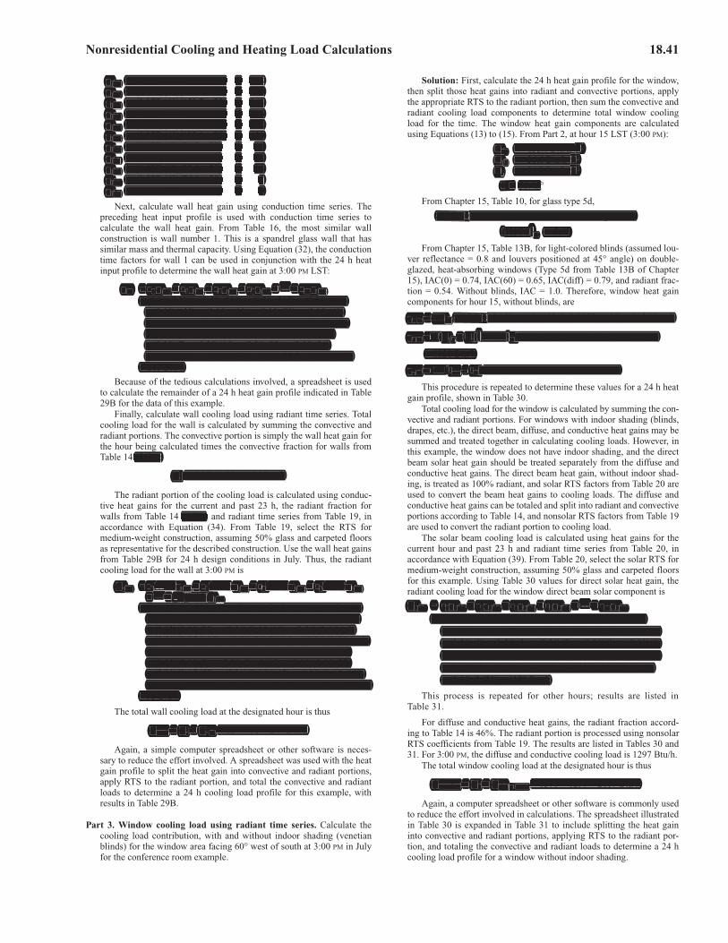
Nonresidential Cooling and Heating Load Calculations 18.41
qi,14 = (0.077)(60)(139.6 – 75) = 298qi,15 = (0.077)(60)(150.7 – 75) = 350qi,16 = (0.077)(60)(153.7 – 75) = 363qi,17 = (0.077)(60)(147.7 – 75) = 336qi,18 = (0.077)(60)(131.7 – 75) = 262qi,19 = (0.077)(60)(103.1 – 75) = 130qi,20 = (0.077)(60)(81.7 – 75) = 31qi,21 = (0.077)(60)(79.8 – 75) = 22qi,22 = (0.077)(60)(78.0 – 75) = 14qi,23 = (0.077)(60)(76.5 – 75) = 7qi,24 = (0.077)(60)(75.1 – 75) = 0
Next, calculate wall heat gain using conduction time series. Thepreceding heat input profile is used with conduction time series tocalculate the wall heat gain. From Table 16, the most similar wallconstruction is wall number 1. This is a spandrel glass wall that hassimilar mass and thermal capacity. Using Equation (32), the conductiontime factors for wall 1 can be used in conjunction with the 24 h heatinput profile to determine the wall heat gain at 3:00 PM LST:
q15 = c0qi,15 + c1qi,14 + c2qi,13 + c3qi,12 + … + c23qi,14
= (0.18)(350) + (0.58)(298) + (0.20)(219) + (0.04)(141)+ (0.00)(122) + (0.00)(100) + (0.00)(73) + (0.00)(42)+ (0.00)(11) + (0.00)(–10) + (0.00)(–17) + (0.00)(–15)+ (0.00)(–12) + (0.00)(–9) + (0.00)(–5) + (0.00)(0)+ (0.00)(7) + (0.00)(14) + (0.00)(22) + (0.00)(31)+ (0.00)(130) + (0.00)(262) + (0.00)(336) + (0.00)(363)
= 285 Btu/h
Because of the tedious calculations involved, a spreadsheet is usedto calculate the remainder of a 24 h heat gain profile indicated in Table29B for the data of this example.
Finally, calculate wall cooling load using radiant time series. Totalcooling load for the wall is calculated by summing the convective andradiant portions. The convective portion is simply the wall heat gain forthe hour being calculated times the convective fraction for walls fromTable 14 (54%):
Qc = (285)(0.54) = 154 Btu/h
The radiant portion of the cooling load is calculated using conduc-tive heat gains for the current and past 23 h, the radiant fraction forwalls from Table 14 (46%), and radiant time series from Table 19, inaccordance with Equation (34). From Table 19, select the RTS formedium-weight construction, assuming 50% glass and carpeted floorsas representative for the described construction. Use the wall heat gainsfrom Table 29B for 24 h design conditions in July. Thus, the radiantcooling load for the wall at 3:00 PM is
Qr,15 = r0(0.46)qi,15 + r1(0.46) qi,14 + r2(0.46) qi,13 + r3(0.46) qi,12+ … + r23(0.46) qi,16
= (0.49)(0.46)(285) + (0.17)(0.46)(214) + (0.09)(0.46)(150)+ (0.05)(0.46)(119) + (0.03)(0.46)(96) + (0.02)(0.46)(69)+ (0.02)(0.46)(39) + (0.01)(0.46)(11) + (0.01)(0.46)(–8)+ (0.01)(0.46)(–15) + (0.01)(0.46)(–14) + (0.01)(0.46)(–12)+ (0.01)(0.46)(–9) + (0.01)(0.46)(–4) + (0.01)(0.46)(1)+ (0.01)(0.46)(8) + (0.01)(0.46)(15) + (0.01)(0.46)(27)+ (0.01)(0.46)(58) + (0.01)(0.46)(147) + (0.00)(0.46)(257)+ (0.00)(0.46)(329) + (0.00) (0.46)(353) + (0.00)(0.46)(337)
= 93 Btu/h
The total wall cooling load at the designated hour is thus
Qwall = Qc + Qr15 = 154 + 93 = 247 Btu/h
Again, a simple computer spreadsheet or other software is neces-sary to reduce the effort involved. A spreadsheet was used with the heatgain profile to split the heat gain into convective and radiant portions,apply RTS to the radiant portion, and total the convective and radiantloads to determine a 24 h cooling load profile for this example, withresults in Table 29B.
Part 3. Window cooling load using radiant time series. Calculate thecooling load contribution, with and without indoor shading (venetianblinds) for the window area facing 60° west of south at 3:00 PM in Julyfor the conference room example.
Solution: First, calculate the 24 h heat gain profile for the window,then split those heat gains into radiant and convective portions, applythe appropriate RTS to the radiant portion, then sum the convective andradiant cooling load components to determine total window coolingload for the time. The window heat gain components are calculatedusing Equations (13) to (15). From Part 2, at hour 15 LST (3:00 PM):
Et,b = 133.6 Btu/h·ft2
Et,d = 36.6 Btu/h·ft2
Er = 25.7 Btu/h·ft2
� = 58.45°
From Chapter 15, Table 10, for glass type 5d,
SHGC(�) = SHGC(58.45) = 0.3978 (interpolated)
SHGC�D = 0.41
From Chapter 15, Table 13B, for light-colored blinds (assumed lou-ver reflectance = 0.8 and louvers positioned at 45° angle) on double-glazed, heat-absorbing windows (Type 5d from Table 13B of Chapter15), IAC(0) = 0.74, IAC(60) = 0.65, IAC(diff) = 0.79, and radiant frac-tion = 0.54. Without blinds, IAC = 1.0. Therefore, window heat gaincomponents for hour 15, without blinds, are
qb15 = AEt,b SHGC(�)(IAC) = (40)(133.6)(0.3978)(1.00) = 2126 Btu/h
qd15 = A(Et,d + Er) SHGC�D(IAC) = (40)(36.6 + 25.7)(0.41)(1.00)
= 1021 Btu/h
qc15 = UA(tout – tin) = (0.56)(40)(91.9 – 75) = 379 Btu/h
This procedure is repeated to determine these values for a 24 h heatgain profile, shown in Table 30.
Total cooling load for the window is calculated by summing the con-vective and radiant portions. For windows with indoor shading (blinds,drapes, etc.), the direct beam, diffuse, and conductive heat gains may besummed and treated together in calculating cooling loads. However, inthis example, the window does not have indoor shading, and the directbeam solar heat gain should be treated separately from the diffuse andconductive heat gains. The direct beam heat gain, without indoor shad-ing, is treated as 100% radiant, and solar RTS factors from Table 20 areused to convert the beam heat gains to cooling loads. The diffuse andconductive heat gains can be totaled and split into radiant and convectiveportions according to Table 14, and nonsolar RTS factors from Table 19are used to convert the radiant portion to cooling load.
The solar beam cooling load is calculated using heat gains for thecurrent hour and past 23 h and radiant time series from Table 20, inaccordance with Equation (39). From Table 20, select the solar RTS formedium-weight construction, assuming 50% glass and carpeted floorsfor this example. Using Table 30 values for direct solar heat gain, theradiant cooling load for the window direct beam solar component is
Qb,15 = r0qb,15 + r1qb,14 + r2qb,13 + r3qb,12 + … + r23qb,16
= (0.54)(2126) + (0.16)(1234) + (0.08)(302) + (0.04)(0)+ (0.03)(0) + (0.02)(0) + (0.01)(0) + (0.01)(0) + (0.01)(0)+ (0.01)(0) + (0.01)(0) + (0.01)(0) + (0.01)(0) + (0.01)(0)+ (0.01)(0) + (0.01)(0) + (0.01)(0) + (0.01)(0) + (0.01)(0)+ (0.00)(0) + (0.00)(865) + (0.00)(2080) + (0.00)(2656)+ (0.00)(2670) = 1370 Btu/h
This process is repeated for other hours; results are listed inTable 31.
For diffuse and conductive heat gains, the radiant fraction accord-ing to Table 14 is 46%. The radiant portion is processed using nonsolarRTS coefficients from Table 19. The results are listed in Tables 30 and31. For 3:00 PM, the diffuse and conductive cooling load is 1297 Btu/h.
The total window cooling load at the designated hour is thus
Qwindow = Qb + Qdiff + cond = 1370 + 1297 = 2667 Btu/h
Again, a computer spreadsheet or other software is commonly usedto reduce the effort involved in calculations. The spreadsheet illustratedin Table 30 is expanded in Table 31 to include splitting the heat gaininto convective and radiant portions, applying RTS to the radiant por-tion, and totaling the convective and radiant loads to determine a 24 hcooling load profile for a window without indoor shading.
qi, = (0.077)(60)(150.7 – 75) = 350,15,qi, = (0.077)(60)(153.7 – 75) = 363,16,qi, = (0.077)(60)(147.7 – 75) = 336,17,qi, = (0.077)(60)(131.7 – 75) = 262,18,qi, = (0.077)(60)(103.1 – 75) = 130,19,qi, = (0.077)(60)(81.7 – 75) = 31,20,qi, = (0.077)(60)(79.8 – 75) = 22,21,qi, = (0.077)(60)(78.0 – 75) = 14,22,qi, = (0.077)(60)(76.5 – 75) = 7,23,qi, = (0.077)(60)(75.1 – 75) =,24 0
qi,, = (0.077)(60)(139.6 – 75) = 298,14,
… q15 = c0qi, + c1qi, + c2qi, + c3qi, + + c23qi,,15 ,14 ,13 ,12 ,14
= (0.18)(350) + (0.58)(298) + (0.20)(219) + (0.04)(141)+ (0.00)(122) + (0.00)(100) + (0.00)(73) + (0.00)(42)+ (0.00)(11) + (0.00)(–10) + (0.00)(–17) + (0.00)(–15)+ (0.00)(–12) + (0.00)(–9) + (0.00)(–5) + (0.00)(0)+ (0.00)(7) + (0.00)(14) + (0.00)(22) + (0.00)(31)+ (0.00)(130) + (0.00)(262) + (0.00)(336) + (0.00)(363)
= 285 Btu/h
(54%):
Qc = (285)(0.54) = 154 Btu/h
(46%),
Qr,rr == r0((0.46))qi, + r1((0.46) qi, + r2r ((0.46) qi, + r3((0.46) qi,r,15r ,15 ,14 ,13 ,120(… + +
,r23r ((0.46) qi,,16,
= (0.49)(0.46)(285) + (0.17)(0.46)(214) + (0.09)(0.46)(150)+ (0.05)(0.46)(119) + (0.03)(0.46)(96) + (0.02)(0.46)(69)+ (0.02)(0.46)(39) + (0.01)(0.46)(11) + (0.01)(0.46)(–8)+ (0.01)(0.46)(–15) + (0.01)(0.46)(–14) + (0.01)(0.46)(–12)+ (0.01)(0.46)(–9) + (0.01)(0.46)(–4) + (0.01)(0.46)(1)+ (0.01)(0.46)(8) + (0.01)(0.46)(15) + (0.01)(0.46)(27)+ (0.01)(0.46)(58) + (0.01)(0.46)(147) + (0.00)(0.46)(257)+ (0.00)(0.46)(329) + (0.00) (0.46)(353) + (0.00)(0.46)(337)
= 93 Btu/h
Qwall l = Qc + Qr15 = 154 + 93 = 247 Btu/h
ft2Et, = 133.6 Btu/h·ft,bft2
,Et, = 36.6 Btu/h·f,d
ft2,
ErE = 25.7 Btu/h·f
� = 58.45°
SHGC(��) = SHGC(58.45) = 0.3978 (interpolated)
� SHGC� = 0.41�D
qb15 = AEt, SHGC(��)(IAC) = (40)(133.6)(0.3978)(1.00) = 2126 Btu/ht,b
��qd15 = A((E(( t, + ErE ) SHGC��D((IAC) = (40)(36.6 + 25.7)(0.41)(1.00),d d
= 1021 Btu/h
qc15 = UA((tout t – tin) = (0.56)(40)(91.9 – 75) = 379 Btu/h
… Qb, = r0qb, + r1qb, + r2qb, + r3qb, + + r23qb,,15 ,15 ,14 ,13 ,12 ,16
= (0.54)(2126) + (0.16)(1234) + (0.08)(302) + (0.04)(0)+ (0.03)(0) + (0.02)(0) + (0.01)(0) + (0.01)(0) + (0.01)(0)+ (0.01)(0) + (0.01)(0) + (0.01)(0) + (0.01)(0) + (0.01)(0)+ (0.01)(0) + (0.01)(0) + (0.01)(0) + (0.01)(0) + (0.01)(0)+ (0.00)(0) + (0.00)(865) + (0.00)(2080) + (0.00)(2656)+ (0.00)(2670) = 1370 Btu/h
Qwindow = Qb + Qdifff = 1370 + 1297 = 2667 Btu/hf + f cond d
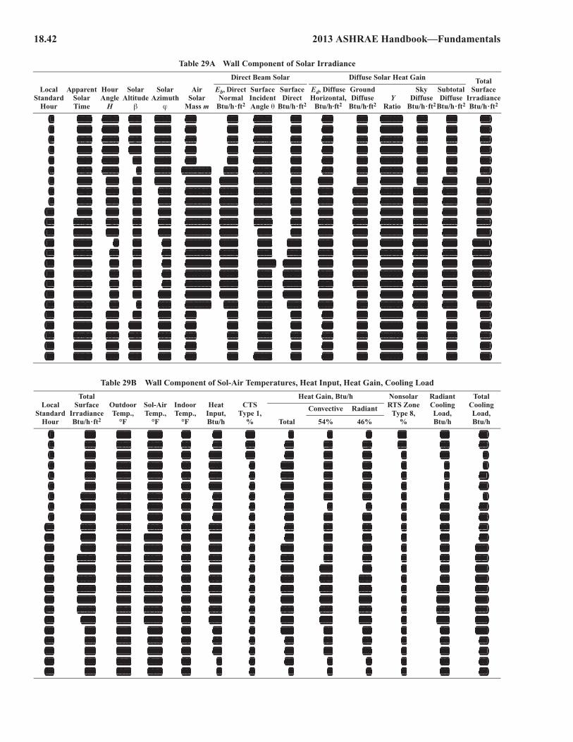
18.42 2013 ASHRAE Handbook—Fundamentals
Table 29A Wall Component of Solar Irradiance
Local Standard
Hour
Apparent Solar Time
Hour Angle
H
Solar Altitude
!
Solar Azimuth
)
AirSolar
Mass m
Direct Beam Solar Diffuse Solar Heat Gain Total Surface
Irradiance Btu/h·ft2
Eb, Direct Normal
Btu/h·ft2
Surface Incident Angle �
Surface Direct
Btu/h·ft2
Ed, Diffuse Horizontal,
Btu/h·ft2
Ground Diffuse
Btu/h·ft2 Y
Ratio
Sky Diffuse
Btu/h·ft2
Subtotal Diffuse
Btu/h·ft2
1 0.26 –176 –36 –175 0.0 0.0 117.4 0.0 0.0 0.0 0.4500 0.0 0.0 0.02 1.26 –161 –33 –159 0.0 0.0 130.9 0.0 0.0 0.0 0.4500 0.0 0.0 0.03 2.26 –146 –27 –144 0.0 0.0 144.5 0.0 0.0 0.0 0.4500 0.0 0.0 0.04 3.26 –131 –19 –132 0.0 0.0 158.1 0.0 0.0 0.0 0.4500 0.0 0.0 0.05 4.26 –116 –9 –122 0.0 0.0 171.3 0.0 0.0 0.0 0.4500 0.0 0.0 0.06 5.26 –101 3 –113 16.91455 16.5 172.5 0.0 5.7 0.6 0.4500 2.6 3.2 3.27 6.26 –86 14 –105 3.98235 130.7 159.5 0.0 19.8 5.2 0.4500 8.9 14.1 14.18 7.26 –71 27 –98 2.22845 193.5 145.9 0.0 29.3 11.6 0.4500 13.2 24.8 24.89 8.26 –56 39 –90 1.58641 228.3 132.3 0.0 36.0 18.0 0.4500 16.2 34.2 34.2
10 9.26 –41 51 –81 1.27776 248.8 118.8 0.0 40.7 23.5 0.4500 18.3 41.8 41.811 10.26 –26 63 –67 1.11740 260.9 105.6 0.0 43.8 27.7 0.4553 19.9 47.6 47.612 11.26 –11 74 –39 1.04214 266.9 92.6 0.0 45.4 30.1 0.5306 24.1 54.2 54.213 12.26 4 76 16 1.02872 268.0 80.2 45.5 45.7 30.6 0.6332 29.0 59.6 105.114 13.26 19 69 57 1.07337 264.3 68.7 96.2 44.7 29.1 0.7505 33.6 62.7 158.815 14.26 34 57 75 1.18905 255.3 58.45 133.6 42.3 25.7 0.8644 36.6 62.3 195.916 15.26 49 45 86 1.41566 239.2 50.4 152.4 38.4 20.7 0.9555 36.7 57.4 209.917 16.26 64 32 94 1.86186 212.2 45.8 148.1 32.7 14.6 1.0073 33.0 47.6 195.718 17.26 79 20 102 2.89735 165.3 45.5 115.8 24.7 8.1 1.0100 24.9 33.1 148.919 18.26 94 8 109 6.84406 76.0 49.7 49.1 13.0 2.4 0.9631 12.5 14.9 64.020 19.26 109 –3 117 0.0 0.0 57.5 0.0 0.0 0.0 0.8755 0.0 0.0 0.021 20.26 124 –14 127 0.0 0.0 67.5 0.0 0.0 0.0 0.7630 0.0 0.0 0.022 21.26 139 –23 138 0.0 0.0 79.0 0.0 0.0 0.0 0.6452 0.0 0.0 0.023 22.26 154 –30 151 0.0 0.0 91.3 0.0 0.0 0.0 0.5403 0.0 0.0 0.024 23.26 169 –35 167 0.0 0.0 104.2 0.0 0.0 0.0 0.4618 0.0 0.0 0.0
Table 29B Wall Component of Sol-Air Temperatures, Heat Input, Heat Gain, Cooling Load
Local Standard
Hour
Total Surface
Irradiance Btu/h·ft2
Outdoor Temp.,
°F
Sol-Air Temp.,
°F
Indoor Temp.,
°F
Heat Input, Btu/h
CTSType 1,
%
Heat Gain, Btu/h Nonsolar RTS Zone
Type 8,%
Radiant Cooling Load, Btu/h
Total Cooling Load, Btu/hTotal
Convective Radiant
54% 46%
1 0.0 73.9 73.9 75 –5 18 1 1 1 49 16 162 0.0 73.0 73.0 75 –9 58 –4 –2 –2 17 12 103 0.0 72.4 72.4 75 –12 20 –9 –5 –4 9 10 54 0.0 71.8 71.8 75 –15 4 –12 –6 –5 5 8 25 0.0 71.4 71.4 75 –17 0 –14 –8 –7 3 7 –16 3.2 71.8 72.8 75 –10 0 –15 –8 –7 2 6 –27 14.1 73.2 77.4 75 11 0 –8 –4 –4 2 7 28 24.8 76.7 84.1 75 42 0 11 6 5 1 11 179 34.2 80.6 90.8 75 73 0 39 21 18 1 18 39
10 41.8 84.1 96.7 75 100 0 69 37 32 1 27 6411 47.6 87.2 101.5 75 122 0 96 52 44 1 36 8812 54.2 89.2 105.5 75 141 0 119 64 55 1 43 10813 105.1 90.9 122.4 75 219 0 150 81 69 1 53 13414 158.8 91.9 139.6 75 298 0 214 115 98 1 71 18615 195.9 91.9 150.7 75 350 0 285 154 131 1 93 24716 209.9 90.7 153.7 75 363 0 337 182 155 1 114 29617 195.7 89.0 147.7 75 336 0 353 191 162 1 127 31818 148.9 87.0 131.7 75 262 0 329 177 151 1 128 30619 64.0 83.9 103.1 75 130 0 257 139 118 1 115 25320 0.0 81.7 81.7 75 31 0 147 79 67 1 86 16521 0.0 79.8 79.8 75 22 0 58 32 27 0 56 8822 0.0 78.0 78.0 75 14 0 27 14 12 0 38 5223 0.0 76.5 76.5 75 7 0 15 8 7 0 27 3524 0.0 75.1 75.1 75 0 0 8 4 4 0 20 25
1 0.26 –176 –36 –175 0.0 0.0 117.4 0.0 0.0 0.0 0.4500 0.0 0.0 0.02 1.26 –161 –33 –159 0.0 0.0 130.9 0.0 0.0 0.0 0.4500 0.0 0.0 0.03 2.26 –146 –27 –144 0.0 0.0 144.5 0.0 0.0 0.0 0.4500 0.0 0.0 0.04 3.26 –131 –19 –132 0.0 0.0 158.1 0.0 0.0 0.0 0.4500 0.0 0.0 0.05 4.26 –116 –9 –122 0.0 0.0 171.3 0.0 0.0 0.0 0.4500 0.0 0.0 0.06 5.26 –101 3 –113 16.91455 16.5 172.5 0.0 5.7 0.6 0.4500 2.6 3.2 3.27 6.26 –86 14 –105 3.98235 130.7 159.5 0.0 19.8 5.2 0.4500 8.9 14.1 14.18 7.26 –71 27 –98 2.22845 193.5 145.9 0.0 29.3 11.6 0.4500 13.2 24.8 24.89 8.26 –56 39 –90 1.58641 228.3 132.3 0.0 36.0 18.0 0.4500 16.2 34.2 34.2
10 9.26 –41 51 –81 1.27776 248.8 118.8 0.0 40.7 23.5 0.4500 18.3 41.8 41.811 10.26 –26 63 –67 1.11740 260.9 105.6 0.0 43.8 27.7 0.4553 19.9 47.6 47.612 11.26 –11 74 –39 1.04214 266.9 92.6 0.0 45.4 30.1 0.5306 24.1 54.2 54.213 12.26 4 76 16 1.02872 268.0 80.2 45.5 45.7 30.6 0.6332 29.0 59.6 105.114 13.26 19 69 57 1.07337 264.3 68.7 96.2 44.7 29.1 0.7505 33.6 62.7 158.815 14.26 34 57 75 1.18905 255.3 58.45 133.6 42.3 25.7 0.8644 36.6 62.3 195.916 15.26 49 45 86 1.41566 239.2 50.4 152.4 38.4 20.7 0.9555 36.7 57.4 209.917 16.26 64 32 94 1.86186 212.2 45.8 148.1 32.7 14.6 1.0073 33.0 47.6 195.718 17.26 79 20 102 2.89735 165.3 45.5 115.8 24.7 8.1 1.0100 24.9 33.1 148.919 18.26 94 8 109 6.84406 76.0 49.7 49.1 13.0 2.4 0.9631 12.5 14.9 64.020 19.26 109 –3 117 0.0 0.0 57.5 0.0 0.0 0.0 0.8755 0.0 0.0 0.021 20.26 124 –14 127 0.0 0.0 67.5 0.0 0.0 0.0 0.7630 0.0 0.0 0.022 21.26 139 –23 138 0.0 0.0 79.0 0.0 0.0 0.0 0.6452 0.0 0.0 0.023 22.26 154 –30 151 0.0 0.0 91.3 0.0 0.0 0.0 0.5403 0.0 0.0 0.024 23.26 169 –35 167 0.0 0.0 104.2 0.0 0.0 0.0 0.4618 0.0 0.0 0.0
1 0.0 73.9 73.9 75 –5 18 1 1 1 49 16 162 0.0 73.0 73.0 75 –9 58 –4 –2 –2 17 12 103 0.0 72.4 72.4 75 –12 20 –9 –5 –4 9 10 54 0.0 71.8 71.8 75 –15 4 –12 –6 –5 5 8 25 0.0 71.4 71.4 75 –17 0 –14 –8 –7 3 7 –16 3.2 71.8 72.8 75 –10 0 –15 –8 –7 2 6 –27 14.1 73.2 77.4 75 11 0 –8 –4 –4 2 7 28 24.8 76.7 84.1 75 42 0 11 6 5 1 11 179 34.2 80.6 90.8 75 73 0 39 21 18 1 18 39
10 41.8 84.1 96.7 75 100 0 69 37 32 1 27 6411 47.6 87.2 101.5 75 122 0 96 52 44 1 36 8812 54.2 89.2 105.5 75 141 0 119 64 55 1 43 10813 105.1 90.9 122.4 75 219 0 150 81 69 1 53 13414 158.8 91.9 139.6 75 298 0 214 115 98 1 71 18615 195.9 91.9 150.7 75 350 0 285 154 131 1 93 24716 209.9 90.7 153.7 75 363 0 337 182 155 1 114 29617 195.7 89.0 147.7 75 336 0 353 191 162 1 127 31818 148.9 87.0 131.7 75 262 0 329 177 151 1 128 30619 64.0 83.9 103.1 75 130 0 257 139 118 1 115 25320 0.0 81.7 81.7 75 31 0 147 79 67 1 86 16521 0.0 79.8 79.8 75 22 0 58 32 27 0 56 8822 0.0 78.0 78.0 75 14 0 27 14 12 0 38 5223 0.0 76.5 76.5 75 7 0 15 8 7 0 27 3524 0.0 75.1 75.1 75 0 0 8 4 4 0 20 25
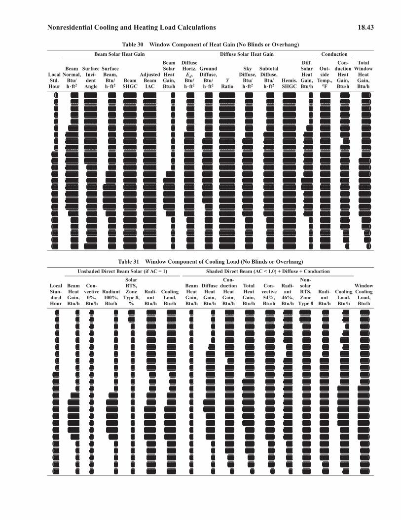
Nonresidential Cooling and Heating Load Calculations 18.43
Table 30 Window Component of Heat Gain (No Blinds or Overhang)
Local Std.
Hour
Beam Solar Heat Gain Diffuse Solar Heat Gain Conduction
Total Window
Heat Gain, Btu/h
Beam Normal,
Btu/h·ft2
Surface Inci-dent
Angle
Surface Beam, Btu/h·ft2
Beam SHGC
Adjusted Beam IAC
Beam SolarHeat Gain, Btu/h
Diffuse Horiz.
Ed,Btu/h·ft2
Ground Diffuse,
Btu/ h·ft2
YRatio
Sky Diffuse,
Btu/h·ft2
Subtotal Diffuse,
Btu/h·ft2
Hemis. SHGC
Diff. Solar Heat Gain, Btu/h
Out-side
Temp.,°F
Con-duction
Heat Gain, Btu/h
1 0.0 117.4 0.0 0.000 1.000 0 0.0 0.0 0.4500 0.0 0.0 0.410 0 73.9 –25 –252 0.0 130.9 0.0 0.000 1.000 0 0.0 0.0 0.4500 0.0 0.0 0.410 0 73.0 –45 –453 0.0 144.5 0.0 0.000 1.000 0 0.0 0.0 0.4500 0.0 0.0 0.410 0 72.4 –58 –584 0.0 158.1 0.0 0.000 1.000 0 0.0 0.0 0.4500 0.0 0.0 0.410 0 71.8 –72 –725 0.0 171.3 0.0 0.000 1.000 0 0.0 0.0 0.4500 0.0 0.0 0.410 0 71.4 –81 –816 16.5 172.5 0.0 0.000 0.000 0 5.7 0.6 0.4500 2.6 3.2 0.410 52 71.8 –72 –197 130.7 159.5 0.0 0.000 0.000 0 19.8 5.2 0.4500 8.9 14.1 0.410 231 73.2 –40 1918 193.5 145.9 0.0 0.000 0.000 0 29.3 11.6 0.4500 13.2 24.8 0.410 406 76.7 38 4449 228.3 132.3 0.0 0.000 0.000 0 36.0 18.0 0.4500 16.2 34.2 0.410 560 80.6 125 686
10 248.8 118.8 0.0 0.000 0.000 0 40.7 23.5 0.4500 18.3 41.8 0.410 686 84.1 204 89011 260.9 105.6 0.0 0.000 0.000 0 43.8 27.7 0.4553 19.9 47.6 0.410 781 87.2 273 105512 266.9 92.6 0.0 0.000 0.000 0 45.4 30.1 0.5306 24.1 54.2 0.410 890 89.2 318 120813 268.0 80.2 45.5 0.166 1.000 302 45.7 30.6 0.6332 29.0 59.6 0.410 977 90.9 356 163514 264.3 68.7 96.2 0.321 1.000 1234 44.7 29.1 0.7505 33.6 62.7 0.410 1028 91.9 379 264015 255.3 58.4 133.6 0.398 1.000 2126 42.3 25.7 0.8644 36.6 62.3 0.410 1021 91.9 379 352616 239.2 50.4 152.4 0.438 1.000 2670 38.4 20.7 0.9555 36.7 57.4 0.410 942 90.7 352 396417 212.2 45.8 148.1 0.448 1.000 2656 32.7 14.6 1.0073 33.0 47.6 0.410 781 89.0 314 375118 165.3 45.5 115.8 0.449 1.000 2080 24.7 8.1 1.0100 24.9 33.1 0.410 542 87.0 269 289219 76.0 49.7 49.1 0.441 1.000 865 13.0 2.4 0.9631 12.5 14.9 0.410 244 83.9 199 130920 0.0 57.5 0.0 0.403 0.000 0 0.0 0.0 0.8755 0.0 0.0 0.410 0 81.7 150 15021 0.0 67.5 0.0 0.330 0.000 0 0.0 0.0 0.7630 0.0 0.0 0.410 0 79.8 108 10822 0.0 79.0 0.0 0.185 0.000 0 0.0 0.0 0.6452 0.0 0.0 0.410 0 78.0 67 6723 0.0 91.3 0.0 0.000 1.000 0 0.0 0.0 0.5403 0.0 0.0 0.410 0 76.5 34 3424 0.0 104.2 0.0 0.000 1.000 0 0.0 0.0 0.4618 0.0 0.0 0.410 0 75.1 2 2
Table 31 Window Component of Cooling Load (No Blinds or Overhang)
Local Stan-dard Hour
Unshaded Direct Beam Solar (if AC = 1) Shaded Direct Beam (AC < 1.0) + Diffuse + Conduction
Window Cooling Load, Btu/h
Beam Heat Gain, Btu/h
Con-vective
0%, Btu/h
Radiant 100%, Btu/h
Solar RTS, Zone
Type 8,%
Radi-ant
Btu/h
Cooling Load, Btu/h
Beam Heat Gain, Btu/h
Diffuse Heat Gain, Btu/h
Con-duction
Heat Gain, Btu/h
Total Heat Gain, Btu/h
Con-vective 54%, Btu/h
Radi-ant
46%, Btu/h
Non-solar RTS, Zone
Type 8
Radi-ant
Btu/h
Cooling Load, Btu/h
1 0 0 0 54 119 119 0 0 –25 –25 –13 –11 49% 59 45 1652 0 0 0 16 119 119 0 0 –45 –45 –24 –21 17% 49 24 1443 0 0 0 8 119 119 0 0 –58 –58 –31 –27 9% 41 9 1294 0 0 0 4 119 119 0 0 –72 –72 –39 –33 5% 32 –6 1135 0 0 0 3 119 119 0 0 –81 –81 –44 –37 3% 25 –19 1006 0 0 0 2 119 119 0 52 –72 –19 –10 –9 2% 32 22 1417 0 0 0 1 119 119 0 231 –40 191 103 88 2% 78 181 3018 0 0 0 1 116 116 0 406 38 444 240 204 1% 148 388 5049 0 0 0 1 104 104 0 560 125 686 370 315 1% 225 596 700
10 0 0 0 1 83 83 0 686 204 890 481 409 1% 300 780 86311 0 0 0 1 56 56 0 781 273 1055 569 485 1% 365 935 99112 0 0 0 1 29 29 0 890 318 1208 652 556 1% 426 1078 110813 302 0 302 1 172 172 0 977 356 1333 720 613 1% 480 1200 137214 1234 0 1234 1 715 715 0 1028 379 1406 759 647 1% 521 1281 199515 2126 0 2126 1 1370 1370 0 1021 379 1400 756 644 1% 541 1297 266616 2670 0 2670 1 1893 1893 0 942 352 1294 699 595 1% 530 1229 312217 2656 0 2656 1 2090 2090 0 781 314 1094 591 503 1% 487 1078 316818 2080 0 2080 1 1890 1890 0 542 269 811 438 373 1% 411 849 273919 865 0 865 1 1211 1211 0 244 199 444 240 204 1% 302 542 175320 0 0 0 0 549 549 0 0 150 150 81 69 1% 196 277 82621 0 0 0 0 322 322 0 0 108 108 58 49 0% 145 203 52522 0 0 0 0 213 213 0 0 67 67 36 31 0% 112 148 36123 0 0 0 0 157 157 0 0 34 34 18 15 0% 89 107 26524 0 0 0 0 128 128 0 0 2 2 1 1 0% 72 73 201
1 0.0 117.4 0.0 0.000 1.000 0 0.0 0.0 0.4500 0.0 0.0 0.410 0 73.9 –25 –252 0.0 130.9 0.0 0.000 1.000 0 0.0 0.0 0.4500 0.0 0.0 0.410 0 73.0 –45 –453 0.0 144.5 0.0 0.000 1.000 0 0.0 0.0 0.4500 0.0 0.0 0.410 0 72.4 –58 –584 0.0 158.1 0.0 0.000 1.000 0 0.0 0.0 0.4500 0.0 0.0 0.410 0 71.8 –72 –725 0.0 171.3 0.0 0.000 1.000 0 0.0 0.0 0.4500 0.0 0.0 0.410 0 71.4 –81 –816 16.5 172.5 0.0 0.000 0.000 0 5.7 0.6 0.4500 2.6 3.2 0.410 52 71.8 –72 –197 130.7 159.5 0.0 0.000 0.000 0 19.8 5.2 0.4500 8.9 14.1 0.410 231 73.2 –40 1918 193.5 145.9 0.0 0.000 0.000 0 29.3 11.6 0.4500 13.2 24.8 0.410 406 76.7 38 4449 228.3 132.3 0.0 0.000 0.000 0 36.0 18.0 0.4500 16.2 34.2 0.410 560 80.6 125 686
10 248.8 118.8 0.0 0.000 0.000 0 40.7 23.5 0.4500 18.3 41.8 0.410 686 84.1 204 89011 260.9 105.6 0.0 0.000 0.000 0 43.8 27.7 0.4553 19.9 47.6 0.410 781 87.2 273 105512 266.9 92.6 0.0 0.000 0.000 0 45.4 30.1 0.5306 24.1 54.2 0.410 890 89.2 318 120813 268.0 80.2 45.5 0.166 1.000 302 45.7 30.6 0.6332 29.0 59.6 0.410 977 90.9 356 163514 264.3 68.7 96.2 0.321 1.000 1234 44.7 29.1 0.7505 33.6 62.7 0.410 1028 91.9 379 264015 255.3 58.4 133.6 0.398 1.000 2126 42.3 25.7 0.8644 36.6 62.3 0.410 1021 91.9 379 352616 239.2 50.4 152.4 0.438 1.000 2670 38.4 20.7 0.9555 36.7 57.4 0.410 942 90.7 352 396417 212.2 45.8 148.1 0.448 1.000 2656 32.7 14.6 1.0073 33.0 47.6 0.410 781 89.0 314 375118 165.3 45.5 115.8 0.449 1.000 2080 24.7 8.1 1.0100 24.9 33.1 0.410 542 87.0 269 289219 76.0 49.7 49.1 0.441 1.000 865 13.0 2.4 0.9631 12.5 14.9 0.410 244 83.9 199 130920 0.0 57.5 0.0 0.403 0.000 0 0.0 0.0 0.8755 0.0 0.0 0.410 0 81.7 150 15021 0.0 67.5 0.0 0.330 0.000 0 0.0 0.0 0.7630 0.0 0.0 0.410 0 79.8 108 10822 0.0 79.0 0.0 0.185 0.000 0 0.0 0.0 0.6452 0.0 0.0 0.410 0 78.0 67 6723 0.0 91.3 0.0 0.000 1.000 0 0.0 0.0 0.5403 0.0 0.0 0.410 0 76.5 34 3424 0.0 104.2 0.0 0.000 1.000 0 0.0 0.0 0.4618 0.0 0.0 0.410 0 75.1 2 2
1 0 0 0 54 119 119 0 0 –25 –25 –13 –11 49% 59 45 1652 0 0 0 16 119 119 0 0 –45 –45 –24 –21 17% 49 24 1443 0 0 0 8 119 119 0 0 –58 –58 –31 –27 9% 41 9 1294 0 0 0 4 119 119 0 0 –72 –72 –39 –33 5% 32 –6 1135 0 0 0 3 119 119 0 0 –81 –81 –44 –37 3% 25 –19 1006 0 0 0 2 119 119 0 52 –72 –19 –10 –9 2% 32 22 1417 0 0 0 1 119 119 0 231 –40 191 103 88 2% 78 181 3018 0 0 0 1 116 116 0 406 38 444 240 204 1% 148 388 5049 0 0 0 1 104 104 0 560 125 686 370 315 1% 225 596 700
10 0 0 0 1 83 83 0 686 204 890 481 409 1% 300 780 86311 0 0 0 1 56 56 0 781 273 1055 569 485 1% 365 935 99112 0 0 0 1 29 29 0 890 318 1208 652 556 1% 426 1078 110813 302 0 302 1 172 172 0 977 356 1333 720 613 1% 480 1200 137214 1234 0 1234 1 715 715 0 1028 379 1406 759 647 1% 521 1281 199515 2126 0 2126 1 1370 1370 0 1021 379 1400 756 644 1% 541 1297 266616 2670 0 2670 1 1893 1893 0 942 352 1294 699 595 1% 530 1229 312217 2656 0 2656 1 2090 2090 0 781 314 1094 591 503 1% 487 1078 316818 2080 0 2080 1 1890 1890 0 542 269 811 438 373 1% 411 849 273919 865 0 865 1 1211 1211 0 244 199 444 240 204 1% 302 542 175320 0 0 0 0 549 549 0 0 150 150 81 69 1% 196 277 82621 0 0 0 0 322 322 0 0 108 108 58 49 0% 145 203 52522 0 0 0 0 213 213 0 0 67 67 36 31 0% 112 148 36123 0 0 0 0 157 157 0 0 34 34 18 15 0% 89 107 26524 0 0 0 0 128 128 0 0 2 2 1 1 0% 72 73 201
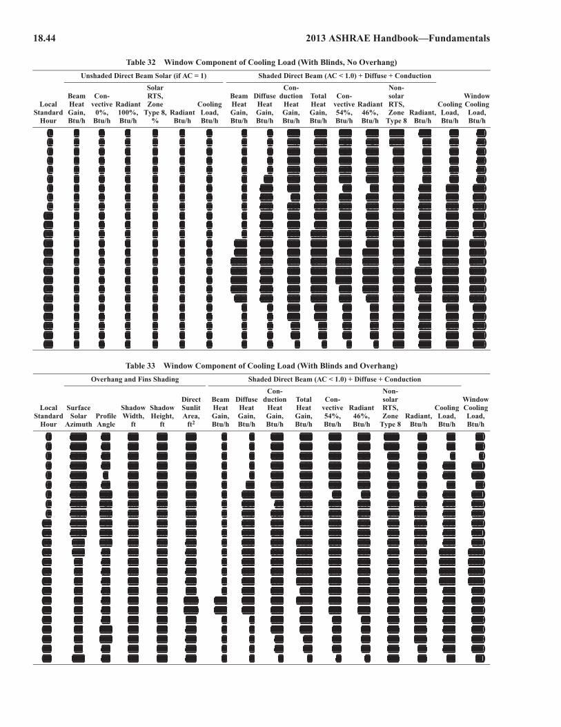
18.44 2013 ASHRAE Handbook—Fundamentals
Table 32 Window Component of Cooling Load (With Blinds, No Overhang)
Local Standard
Hour
Unshaded Direct Beam Solar (if AC = 1) Shaded Direct Beam (AC < 1.0) + Diffuse + Conduction
Window Cooling Load, Btu/h
Beam Heat Gain, Btu/h
Con-vective
0%, Btu/h
Radiant 100%, Btu/h
Solar RTS, Zone
Type 8,%
Radiant Btu/h
Cooling Load, Btu/h
Beam Heat Gain, Btu/h
Diffuse Heat Gain, Btu/h
Con-duction
Heat Gain, Btu/h
Total Heat Gain, Btu/h
Con-vective 54%, Btu/h
Radiant 46%, Btu/h
Non-solar RTS, Zone
Type 8Radiant,
Btu/h
Cooling Load, Btu/h
1 0 0 0 1 0 0 0 0 –25 –25 –11 –13 49% 105 94 942 0 0 0 0 0 0 0 0 –45 –45 –21 –24 17% 90 70 703 0 0 0 0 0 0 0 0 –58 –58 –27 –31 9% 81 54 544 0 0 0 0 0 0 0 0 –72 –72 –33 –39 5% 72 39 395 0 0 0 0 0 0 0 0 –81 –81 –37 –44 3% 63 26 266 0 0 0 0 0 0 0 41 –72 –30 –14 –16 2% 70 56 567 0 0 0 0 0 0 0 183 –40 143 66 77 2% 114 180 1808 0 0 0 0 0 0 0 321 38 359 165 194 1% 183 348 3489 0 0 0 0 0 0 0 443 125 568 261 307 1% 260 522 522
10 0 0 0 0 0 0 0 542 204 746 343 403 1% 331 674 67411 0 0 0 0 0 0 0 617 273 891 410 481 1% 391 801 80112 0 0 0 0 0 0 0 703 318 1021 470 551 1% 443 913 91313 0 0 0 0 0 0 196 772 356 1325 609 715 1% 540 1149 114914 0 0 0 0 0 0 802 812 379 1992 916 1076 1% 751 1668 166815 0 0 0 0 0 0 1388 807 379 2574 1184 1390 1% 987 2171 217116 0 0 0 0 0 0 1784 744 352 2880 1325 1555 1% 1170 2495 249517 0 0 0 0 0 0 1816 617 314 2747 1263 1483 1% 1221 2484 248418 0 0 0 0 0 0 1458 428 269 2156 992 1164 1% 1103 2094 209419 0 0 0 0 0 0 624 193 199 1017 468 549 1% 774 1242 124220 0 0 0 0 0 0 0 0 150 150 69 81 1% 434 503 50321 0 0 0 0 0 0 0 0 108 108 49 58 0% 290 339 33922 0 0 0 0 0 0 0 0 67 67 31 36 0% 209 240 24023 0 0 0 0 0 0 0 0 34 34 15 18 0% 160 176 17624 0 0 0 0 0 0 0 0 2 2 1 1 0% 128 129 129
Table 33 Window Component of Cooling Load (With Blinds and Overhang)
Local Standard
Hour
Overhang and Fins Shading Shaded Direct Beam (AC < 1.0) + Diffuse + Conduction
Window Cooling Load, Btu/h
Surface Solar
AzimuthProfile Angle
Shadow Width,
ft
Shadow Height,
ft
Direct Sunlit Area,
ft2
Beam Heat Gain, Btu/h
Diffuse Heat Gain, Btu/h
Con-duction
Heat Gain, Btu/h
Total Heat Gain, Btu/h
Con-vective 54%, Btu/h
Radiant 46%, Btu/h
Non-solar RTS, Zone
Type 8Radiant,
Btu/h
Cooling Load, Btu/h
1 –235 52 0.0 0.0 0.0 0 0 –25 –25 –13 –11 49% 55 42 422 –219 40 0.0 0.0 0.0 0 0 –45 –45 –24 –21 17% 43 19 193 –204 29 0.0 0.0 0.0 0 0 –58 –58 –31 –27 9% 36 4 44 –192 19 0.0 0.0 0.0 0 0 –72 –72 –39 –33 5% 28 –11 –115 –182 9 0.0 0.0 0.0 0 0 –81 –81 –44 –37 3% 20 –23 –236 –173 –3 0.0 0.0 0.0 0 41 –72 –30 –16 –14 2% 26 10 107 –165 –15 0.0 0.0 0.0 0 183 –40 143 77 66 2% 64 141 1418 –158 –28 0.0 0.0 0.0 0 321 38 359 194 165 1% 122 316 3169 –150 –43 0.0 0.0 0.0 0 443 125 568 307 261 1% 189 496 496
10 –141 –58 0.0 0.0 0.0 0 542 204 746 403 343 1% 253 656 65611 –127 –73 0.0 0.0 0.0 0 617 273 891 481 410 1% 310 791 79112 –99 –87 0.0 0.0 0.0 0 703 318 1021 551 470 1% 363 914 91413 –44 80 0.0 6.4 0.0 0 772 356 1128 609 519 1% 409 1018 101814 –3 69 0.0 6.4 0.0 0 812 379 1190 643 548 1% 443 1085 108515 15 58 0.0 6.4 0.0 0 807 379 1186 640 545 1% 457 1098 109816 26 48 0.0 6.4 0.0 0 744 352 1096 592 504 1% 449 1040 104017 34 38 0.0 6.4 0.0 0 617 314 930 502 428 1% 412 915 91518 42 26 0.0 4.9 18.9 344 428 269 1041 562 479 1% 427 990 99019 49 12 0.0 2.2 53.0 414 193 199 806 435 371 1% 380 816 81620 57 –6 0.0 0.0 0.0 0 0 150 150 81 69 1% 219 300 30021 67 –32 0.0 0.0 0.0 0 0 108 108 58 49 0% 154 212 21222 78 –64 0.0 0.0 0.0 0 0 67 67 36 31 0% 113 150 15023 91 87 0.0 0.0 0.0 0 0 34 34 18 15 0% 87 106 10624 107 67 0.0 0.0 0.0 0 0 2 2 1 1 0% 70 71 71
1 0 0 0 1 0 0 0 0 –25 –25 –11 –13 49% 105 94 942 0 0 0 0 0 0 0 0 –45 –45 –21 –24 17% 90 70 703 0 0 0 0 0 0 0 0 –58 –58 –27 –31 9% 81 54 544 0 0 0 0 0 0 0 0 –72 –72 –33 –39 5% 72 39 395 0 0 0 0 0 0 0 0 –81 –81 –37 –44 3% 63 26 266 0 0 0 0 0 0 0 41 –72 –30 –14 –16 2% 70 56 567 0 0 0 0 0 0 0 183 –40 143 66 77 2% 114 180 1808 0 0 0 0 0 0 0 321 38 359 165 194 1% 183 348 3489 0 0 0 0 0 0 0 443 125 568 261 307 1% 260 522 522
10 0 0 0 0 0 0 0 542 204 746 343 403 1% 331 674 67411 0 0 0 0 0 0 0 617 273 891 410 481 1% 391 801 80112 0 0 0 0 0 0 0 703 318 1021 470 551 1% 443 913 91313 0 0 0 0 0 0 196 772 356 1325 609 715 1% 540 1149 114914 0 0 0 0 0 0 802 812 379 1992 916 1076 1% 751 1668 166815 0 0 0 0 0 0 1388 807 379 2574 1184 1390 1% 987 2171 217116 0 0 0 0 0 0 1784 744 352 2880 1325 1555 1% 1170 2495 249517 0 0 0 0 0 0 1816 617 314 2747 1263 1483 1% 1221 2484 248418 0 0 0 0 0 0 1458 428 269 2156 992 1164 1% 1103 2094 209419 0 0 0 0 0 0 624 193 199 1017 468 549 1% 774 1242 124220 0 0 0 0 0 0 0 0 150 150 69 81 1% 434 503 50321 0 0 0 0 0 0 0 0 108 108 49 58 0% 290 339 33922 0 0 0 0 0 0 0 0 67 67 31 36 0% 209 240 24023 0 0 0 0 0 0 0 0 34 34 15 18 0% 160 176 17624 0 0 0 0 0 0 0 0 2 2 1 1 0% 128 129 129
1 –235 52 0.0 0.0 0.0 0 0 –25 –25 –13 –11 49% 55 42 422 –219 40 0.0 0.0 0.0 0 0 –45 –45 –24 –21 17% 43 19 193 –204 29 0.0 0.0 0.0 0 0 –58 –58 –31 –27 9% 36 4 44 –192 19 0.0 0.0 0.0 0 0 –72 –72 –39 –33 5% 28 –11 –115 –182 9 0.0 0.0 0.0 0 0 –81 –81 –44 –37 3% 20 –23 –236 –173 –3 0.0 0.0 0.0 0 41 –72 –30 –16 –14 2% 26 10 107 –165 –15 0.0 0.0 0.0 0 183 –40 143 77 66 2% 64 141 1418 –158 –28 0.0 0.0 0.0 0 321 38 359 194 165 1% 122 316 3169 –150 –43 0.0 0.0 0.0 0 443 125 568 307 261 1% 189 496 496
10 –141 –58 0.0 0.0 0.0 0 542 204 746 403 343 1% 253 656 65611 –127 –73 0.0 0.0 0.0 0 617 273 891 481 410 1% 310 791 79112 –99 –87 0.0 0.0 0.0 0 703 318 1021 551 470 1% 363 914 91413 –44 80 0.0 6.4 0.0 0 772 356 1128 609 519 1% 409 1018 101814 –3 69 0.0 6.4 0.0 0 812 379 1190 643 548 1% 443 1085 108515 15 58 0.0 6.4 0.0 0 807 379 1186 640 545 1% 457 1098 109816 26 48 0.0 6.4 0.0 0 744 352 1096 592 504 1% 449 1040 104017 34 38 0.0 6.4 0.0 0 617 314 930 502 428 1% 412 915 91518 42 26 0.0 4.9 18.9 344 428 269 1041 562 479 1% 427 990 99019 49 12 0.0 2.2 53.0 414 193 199 806 435 371 1% 380 816 81620 57 –6 0.0 0.0 0.0 0 0 150 150 81 69 1% 219 300 30021 67 –32 0.0 0.0 0.0 0 0 108 108 58 49 0% 154 212 21222 78 –64 0.0 0.0 0.0 0 0 67 67 36 31 0% 113 150 15023 91 87 0.0 0.0 0.0 0 0 34 34 18 15 0% 87 106 10624 107 67 0.0 0.0 0.0 0 0 2 2 1 1 0% 70 71 71
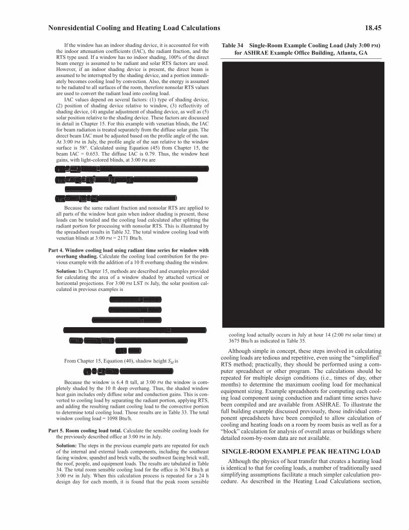
Nonresidential Cooling and Heating Load Calculations 18.45
If the window has an indoor shading device, it is accounted for withthe indoor attenuation coefficients (IAC), the radiant fraction, and theRTS type used. If a window has no indoor shading, 100% of the directbeam energy is assumed to be radiant and solar RTS factors are used.However, if an indoor shading device is present, the direct beam isassumed to be interrupted by the shading device, and a portion immedi-ately becomes cooling load by convection. Also, the energy is assumedto be radiated to all surfaces of the room, therefore nonsolar RTS valuesare used to convert the radiant load into cooling load.
IAC values depend on several factors: (1) type of shading device,(2) position of shading device relative to window, (3) reflectivity ofshading device, (4) angular adjustment of shading device, as well as (5)solar position relative to the shading device. These factors are discussedin detail in Chapter 15. For this example with venetian blinds, the IACfor beam radiation is treated separately from the diffuse solar gain. Thedirect beam IAC must be adjusted based on the profile angle of the sun.At 3:00 PM in July, the profile angle of the sun relative to the windowsurface is 58°. Calculated using Equation (45) from Chapter 15, thebeam IAC = 0.653. The diffuse IAC is 0.79. Thus, the window heatgains, with light-colored blinds, at 3:00 PM are
qb15 = AED SHGC(�)(IAC) = (40)(133.6)(0.3978)(0.653) = 1388 Btu/h
qd15 = A(Ed + Er) SHGC�D(IAC)D= (40)(36.6 + 25.7)(0.41)(0.79)
= 807 Btu/h
qc15 = UA(tout – tin) = (0.56)(40)(91.9 – 75) = 379 Btu/h
Because the same radiant fraction and nonsolar RTS are applied toall parts of the window heat gain when indoor shading is present, thoseloads can be totaled and the cooling load calculated after splitting theradiant portion for processing with nonsolar RTS. This is illustrated bythe spreadsheet results in Table 32. The total window cooling load withvenetian blinds at 3:00 PM = 2171 Btu/h.
Part 4. Window cooling load using radiant time series for window withoverhang shading. Calculate the cooling load contribution for the pre-vious example with the addition of a 10 ft overhang shading the window.
Solution: In Chapter 15, methods are described and examples providedfor calculating the area of a window shaded by attached vertical orhorizontal projections. For 3:00 PM LST IN July, the solar position cal-culated in previous examples is
Solar altitude ! = 57.2°
Solar azimuth "�* 75.1°
Surface-solar azimuth # = 15.1°
From Chapter 15, Equation (106), profile angle � is calculated by
tan � = tan !/cos # = tan(57.2)/cos(15.1) = 1.6087
� = 58.1°
From Chapter 15, Equation (40), shadow height SH is
SH = PH tan � = 10(1.6087) = 16.1 ft
Because the window is 6.4 ft tall, at 3:00 PM the window is com-pletely shaded by the 10 ft deep overhang. Thus, the shaded windowheat gain includes only diffuse solar and conduction gains. This is con-verted to cooling load by separating the radiant portion, applying RTS,and adding the resulting radiant cooling load to the convective portionto determine total cooling load. Those results are in Table 33. The totalwindow cooling load = 1098 Btu/h.
Part 5. Room cooling load total. Calculate the sensible cooling loads forthe previously described office at 3:00 PM in July.
Solution: The steps in the previous example parts are repeated for eachof the internal and external loads components, including the southeastfacing window, spandrel and brick walls, the southwest facing brick wall,the roof, people, and equipment loads. The results are tabulated in Table34. The total room sensible cooling load for the office is 3674 Btu/h at3:00 PM in July. When this calculation process is repeated for a 24 hdesign day for each month, it is found that the peak room sensible
cooling load actually occurs in July at hour 14 (2:00 PM solar time) at3675 Btu/h as indicated in Table 35.
Although simple in concept, these steps involved in calculatingcooling loads are tedious and repetitive, even using the “simplified”RTS method; practically, they should be performed using a com-puter spreadsheet or other program. The calculations should berepeated for multiple design conditions (i.e., times of day, othermonths) to determine the maximum cooling load for mechanicalequipment sizing. Example spreadsheets for computing each cool-ing load component using conduction and radiant time series havebeen compiled and are available from ASHRAE. To illustrate thefull building example discussed previously, those individual com-ponent spreadsheets have been compiled to allow calculation ofcooling and heating loads on a room by room basis as well as for a“block” calculation for analysis of overall areas or buildings wheredetailed room-by-room data are not available.
SINGLE-ROOM EXAMPLE PEAK HEATING LOADAlthough the physics of heat transfer that creates a heating load
is identical to that for cooling loads, a number of traditionally usedsimplifying assumptions facilitate a much simpler calculation pro-cedure. As described in the Heating Load Calculations section,
Table 34 Single-Room Example Cooling Load (July 3:00 PM) for ASHRAE Example Office Building, Atlanta, GA
qb15 = AEDE SHGC(��)(IAC) = (40)(133.6)(0.3978)(0.653) = 1388 Btu/h
�� qd15 = A((E(( dE d + ErE ) SHGC��D((IAC))D= (40)(36.6 + 25.7)(0.41)(0.79)
= 807 Btu/h
qc15 = UA((tout t – tin) = (0.56)(40)(91.9 – 75) = 379 Btu/h
Solar altitude ! = 57.2°
Solar azimuth "�* 75.1°
Surface-solar azimuth # = 15.1°
From Chapter 15, Equation (106), profile angle � is calculated by
tan � = tan !!/cos # = tan(57.2)/cos(15.1) = 1.6087
� = 58.1°
SHS = PHPH tan � = 10(1.6087) = 16.1 ft
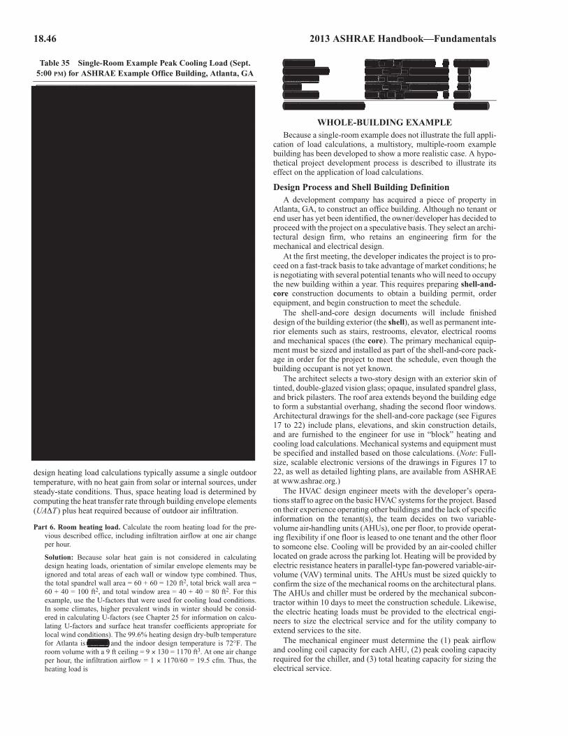
18.46 2013 ASHRAE Handbook—Fundamentals
design heating load calculations typically assume a single outdoortemperature, with no heat gain from solar or internal sources, understeady-state conditions. Thus, space heating load is determined bycomputing the heat transfer rate through building envelope elements(UAT) plus heat required because of outdoor air infiltration.
Part 6. Room heating load. Calculate the room heating load for the pre-vious described office, including infiltration airflow at one air changeper hour.
Solution: Because solar heat gain is not considered in calculatingdesign heating loads, orientation of similar envelope elements may beignored and total areas of each wall or window type combined. Thus,the total spandrel wall area = 60 + 60 = 120 ft2, total brick wall area =60 + 40 = 100 ft2, and total window area = 40 + 40 = 80 ft2. For thisexample, use the U-factors that were used for cooling load conditions.In some climates, higher prevalent winds in winter should be consid-ered in calculating U-factors (see Chapter 25 for information on calcu-lating U-factors and surface heat transfer coefficients appropriate forlocal wind conditions). The 99.6% heating design dry-bulb temperaturefor Atlanta is 21.5°F and the indoor design temperature is 72°F. Theroom volume with a 9 ft ceiling = 9��130 = 1170 ft3. At one air changeper hour, the infiltration airflow = 1��1170/60 = 19.5 cfm. Thus, theheating load is
WHOLE-BUILDING EXAMPLEBecause a single-room example does not illustrate the full appli-
cation of load calculations, a multistory, multiple-room examplebuilding has been developed to show a more realistic case. A hypo-thetical project development process is described to illustrate itseffect on the application of load calculations.
Design Process and Shell Building DefinitionA development company has acquired a piece of property in
Atlanta, GA, to construct an office building. Although no tenant orend user has yet been identified, the owner/developer has decided toproceed with the project on a speculative basis. They select an archi-tectural design firm, who retains an engineering firm for themechanical and electrical design.
At the first meeting, the developer indicates the project is to pro-ceed on a fast-track basis to take advantage of market conditions; heis negotiating with several potential tenants who will need to occupythe new building within a year. This requires preparing shell-and-core construction documents to obtain a building permit, orderequipment, and begin construction to meet the schedule.
The shell-and-core design documents will include finisheddesign of the building exterior (the shell), as well as permanent inte-rior elements such as stairs, restrooms, elevator, electrical roomsand mechanical spaces (the core). The primary mechanical equip-ment must be sized and installed as part of the shell-and-core pack-age in order for the project to meet the schedule, even though thebuilding occupant is not yet known.
The architect selects a two-story design with an exterior skin oftinted, double-glazed vision glass; opaque, insulated spandrel glass,and brick pilasters. The roof area extends beyond the building edgeto form a substantial overhang, shading the second floor windows.Architectural drawings for the shell-and-core package (see Figures17 to 22) include plans, elevations, and skin construction details,and are furnished to the engineer for use in “block” heating andcooling load calculations. Mechanical systems and equipment mustbe specified and installed based on those calculations. (Note: Full-size, scalable electronic versions of the drawings in Figures 17 to22, as well as detailed lighting plans, are available from ASHRAEat www.ashrae.org.)
The HVAC design engineer meets with the developer’s opera-tions staff to agree on the basic HVAC systems for the project. Basedon their experience operating other buildings and the lack of specificinformation on the tenant(s), the team decides on two variable-volume air-handling units (AHUs), one per floor, to provide operat-ing flexibility if one floor is leased to one tenant and the other floorto someone else. Cooling will be provided by an air-cooled chillerlocated on grade across the parking lot. Heating will be provided byelectric resistance heaters in parallel-type fan-powered variable-air-volume (VAV) terminal units. The AHUs must be sized quickly toconfirm the size of the mechanical rooms on the architectural plans.The AHUs and chiller must be ordered by the mechanical subcon-tractor within 10 days to meet the construction schedule. Likewise,the electric heating loads must be provided to the electrical engi-neers to size the electrical service and for the utility company toextend services to the site.
The mechanical engineer must determine the (1) peak airflowand cooling coil capacity for each AHU, (2) peak cooling capacityrequired for the chiller, and (3) total heating capacity for sizing theelectrical service.
Table 35 Single-Room Example Peak Cooling Load (Sept. 5:00 PM) for ASHRAE Example Office Building, Atlanta, GA
Windows: 0.56��80��(72 – 21.5) = 2262 Btu/hSpandrel Wall: 0.077��120��(72 – 21.5) = 467Brick Wall: 0.08��100��(72 – 21.5) = 404Roof: 0.032��130��(72 – 21.5) = 210Infiltration: 19.5��1.1��(72 – 21.5) = 1083
Total Room Heating Load: 4426 Btu/h
21.5°F
Windows: 0.56��800��((72 – 21.5) = 2262 Btu/hSpandrel Wall: 0.077��1200��(
)(72 – 21.5) = 467p
Brick Wall: 0.08��1000� (( )
(72 – 21.5) = 404Roof: 0.032 130
(0 (
)(72 – 21.5) = 210
Infiltration: 19.5� 1.11��((
(72 – 21.5) = 1083
Total Room Heating Load: 4426 Btu/h
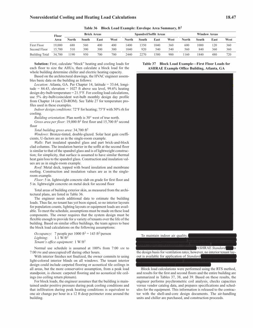
Nonresidential Cooling and Heating Load Calculations 18.47
Solution: First, calculate “block” heating and cooling loads foreach floor to size the AHUs, then calculate a block load for thewhole building determine chiller and electric heating capacity.
Based on the architectural drawings, the HVAC engineer assem-bles basic data on the building as follows:
Location: Atlanta, GA. Per Chapter 14, latitude = 33.64, longi-tude = 84.43, elevation = 1027 ft above sea level, 99.6% heatingdesign dry-bulb temperature = 21.5°F. For cooling load calculations,use 5% dry-bulb/coincident wet-bulb monthly design day profilefrom Chapter 14 (on CD-ROM). See Table 27 for temperature pro-files used in these examples.
Indoor design conditions: 72°F for heating; 75°F with 50% rh forcooling.
Building orientation: Plan north is 30° west of true north.Gross area per floor: 19,000 ft2 first floor and 15,700 ft2 second
floorTotal building gross area: 34,700 ft2
Windows: Bronze-tinted, double-glazed. Solar heat gain coeffi-cients, U-factors are as in the single-room example.
Walls: Part insulated spandrel glass and part brick-and-blockclad columns. The insulation barrier in the soffit at the second flooris similar to that of the spandrel glass and is of lightweight construc-tion; for simplicity, that surface is assumed to have similar thermalheat gain/loss to the spandrel glass. Construction and insulation val-ues are as in single-room example.
Roof: Metal deck, topped with board insulation and membraneroofing. Construction and insulation values are as in the single-room example.
Floor: 5 in. lightweight concrete slab on grade for first floor and5 in. lightweight concrete on metal deck for second floor
Total areas of building exterior skin, as measured from the archi-tectural plans, are listed in Table 36.
The engineer needs additional data to estimate the buildingloads. Thus far, no tenant has yet been signed, so no interior layoutsfor population counts, lighting layouts or equipment loads are avail-able. To meet the schedule, assumptions must be made on these loadcomponents. The owner requires that the system design must beflexible enough to provide for a variety of tenants over the life of thebuilding. Based on similar office buildings, the team agrees to basethe block load calculations on the following assumptions:
Occupancy: 7 people per 1000 ft2 = 143 ft2/personLighting: 1.1 W/ft2
Tenant’s office equipment: 1 W/ft2
Normal use schedule is assumed at 100% from 7:00 AM to7:00 PM and unoccupied/off during other hours.
With interior finishes not finalized, the owner commits to usinglight-colored interior blinds on all windows. The tenant interiordesign could include carpeted flooring or acoustical tile ceilings inall areas, but the more conservative assumption, from a peak loadstandpoint, is chosen: carpeted flooring and no acoustical tile ceil-ings (no ceiling return plenum).
For block loads, the engineer assumes that the building is main-tained under positive pressure during peak cooling conditions andthat infiltration during peak heating conditions is equivalent toone air change per hour in a 12 ft deep perimeter zone around thebuilding.
To maintain indoor air quality, outdoor air must be introducedinto the building. Air will be ducted from roof intake hoods to theAHUs where it will be mixed with return air before being cooled anddehumidified by the AHU’s cooling coil. ASHRAE Standard 62.1 isthe design basis for ventilation rates; however, no interior tenant lay-out is available for application of Standard 62.1 procedures. Basedon past experience, the engineer decides to use 20 cfm of outdoor airper person for sizing the cooling coils and chiller.
Block load calculations were performed using the RTS method,and results for the first and second floors and the entire building aresummarized in Tables 37, 38, and 39. Based on these results, theengineer performs psychrometric coil analysis, checks capacitiesversus vendor catalog data, and prepares specifications and sched-ules for the equipment. This information is released to the contrac-tor with the shell-and-core design documents. The air-handlingunits and chiller are purchased, and construction proceeds.
Table 36 Block Load Example: Envelope Area Summary, ft2
Floor Area
Brick Areas Spandrel/Soffit Areas Window Areas
North South East West North South East West North South East West
First Floor 19,000 680 560 400 400 1400 1350 1040 360 600 1000 120 360Second Floor 15,700 510 390 300 300 1040 920 540 540 560 840 360 360
Building Total 34,700 1190 950 700 700 2440 2270 1580 900 1160 1840 480 720
Table 37 Block Load Example—First Floor Loads for ASHRAE Example Office Building, Atlanta, GA
outdoor air must be introducedinto the building. Air will be ducted from roof intake hoods to theAHUs where it will be mixed with return air before being cooled anddehumidified by the AHU’s cooling coil. A d 62.1 id
62.1 procedures. Basedon past experience, the engineer decides to use 20 cfm of outdoor airper person for sizing the cooling coils and chiller.
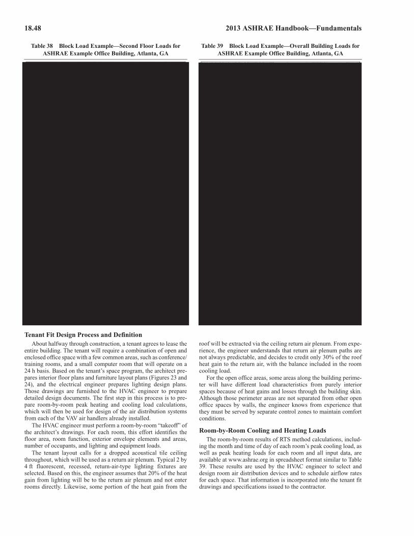
18.48 2013 ASHRAE Handbook—Fundamentals
Tenant Fit Design Process and DefinitionAbout halfway through construction, a tenant agrees to lease the
entire building. The tenant will require a combination of open andenclosed office space with a few common areas, such as conference/training rooms, and a small computer room that will operate on a24 h basis. Based on the tenant’s space program, the architect pre-pares interior floor plans and furniture layout plans (Figures 23 and24), and the electrical engineer prepares lighting design plans.Those drawings are furnished to the HVAC engineer to preparedetailed design documents. The first step in this process is to pre-pare room-by-room peak heating and cooling load calculations,which will then be used for design of the air distribution systemsfrom each of the VAV air handlers already installed.
The HVAC engineer must perform a room-by-room “takeoff” ofthe architect’s drawings. For each room, this effort identifies thefloor area, room function, exterior envelope elements and areas,number of occupants, and lighting and equipment loads.
The tenant layout calls for a dropped acoustical tile ceilingthroughout, which will be used as a return air plenum. Typical 2 by4 ft fluorescent, recessed, return-air-type lighting fixtures areselected. Based on this, the engineer assumes that 20% of the heatgain from lighting will be to the return air plenum and not enterrooms directly. Likewise, some portion of the heat gain from the
roof will be extracted via the ceiling return air plenum. From expe-rience, the engineer understands that return air plenum paths arenot always predictable, and decides to credit only 30% of the roofheat gain to the return air, with the balance included in the roomcooling load.
For the open office areas, some areas along the building perime-ter will have different load characteristics from purely interiorspaces because of heat gains and losses through the building skin.Although those perimeter areas are not separated from other openoffice spaces by walls, the engineer knows from experience thatthey must be served by separate control zones to maintain comfortconditions.
Room-by-Room Cooling and Heating LoadsThe room-by-room results of RTS method calculations, includ-
ing the month and time of day of each room’s peak cooling load, aswell as peak heating loads for each room and all input data, areavailable at www.ashrae.org in spreadsheet format similar to Table39. These results are used by the HVAC engineer to select anddesign room air distribution devices and to schedule airflow ratesfor each space. That information is incorporated into the tenant fitdrawings and specifications issued to the contractor.
Table 38 Block Load Example—Second Floor Loads for ASHRAE Example Office Building, Atlanta, GA
Table 39 Block Load Example—Overall Building Loads for ASHRAE Example Office Building, Atlanta, GA
Nonresidential Cooling and Heating Load Calculations 18.49
ConclusionsThe example results illustrate issues which should be understood
and accounted for in calculating heating and cooling loads:
• First, peak room cooling loads occur at different months andtimes depending on the exterior exposure of the room. Calcula-tion of cooling loads for a single point in time may miss the peakand result in inadequate cooling for that room.
• Often, in real design processes, all data is not known. Reasonableassumptions based on past experience must be made.
• Heating and air-conditioning systems often serve spaces whose usechanges over the life of a building. Assumptions used in heatingand cooling load calculations should consider reasonable possibleuses over the life of the building, not just the first use of the space.
• The relative importance of each cooling and heating load compo-nent varies depending on the portion of the building being con-sidered. Characteristics of a particular window may have littleeffect on the entire building load, but could have a significanteffect on the supply airflow to the room where the window islocated and thus on the comfort of the occupants of that space.
PREVIOUS COOLING LOAD CALCULATION METHODS
Procedures described in this chapter are the most current and sci-entifically derived means for estimating cooling load for a definedbuilding space, but methods in earlier editions of the ASHRAEHandbook are valid for many applications. These earlier proceduresare simplifications of the heat balance principles, and their userequires experience to deal with atypical or unusual circumstances.In fact, any cooling or heating load estimate is no better than theassumptions used to define conditions and parameters such as phys-ical makeup of the various envelope surfaces, conditions of occu-pancy and use, and ambient weather conditions. Experience of thepractitioner can never be ignored.
The primary difference between the HB and RTS methods andthe older methods is the newer methods’ direct approach, comparedto the simplifications necessitated by the limited computer capabil-ity available previously.
The transfer function method (TFM), for example, requiredmany calculation steps. It was originally designed for energy anal-ysis with emphasis on daily, monthly, and annual energy use, andthus was more oriented to average hourly cooling loads than peakdesign loads.
The total equivalent temperature differential method withtime averaging (TETD/TA) has been a highly reliable (if subjec-tive) method of load estimating since its initial presentation in the1967 Handbook of Fundamentals. Originally intended as a manualmethod of calculation, it proved suitable only as a computer appli-cation because of the need to calculate an extended profile of hourlyheat gain values, from which radiant components had to be averagedover a time representative of the general mass of the buildinginvolved. Because perception of thermal storage characteristics of agiven building is almost entirely subjective, with little specific infor-mation for the user to judge variations, the TETD/TA method’s pri-mary usefulness has always been to the experienced engineer.
The cooling load temperature differential method with solarcooling load factors (CLTD/CLF) attempted to simplify the two-step TFM and TETD/TA methods into a single-step technique thatproceeded directly from raw data to cooling load without inter-mediate conversion of radiant heat gain to cooling load. A series offactors were taken from cooling load calculation results (producedby more sophisticated methods) as “cooling load temperature dif-ferences” and “cooling load factors” for use in traditional conduc-tion (q = UAt) equations. The results are approximate cooling loadvalues rather than simple heat gain values. The simplifications and
assumptions used in the original work to derive those factors limitthis method’s applicability to those building types and conditionsfor which the CLTD/CLF factors were derived; the method shouldnot be used beyond the range of applicability.
Although the TFM, TETD/TA, and CLTD/CLF procedures arenot republished in this chapter, those methods are not invalidated ordiscredited. Experienced engineers have successfully used them inmillions of buildings around the world. The accuracy of coolingload calculations in practice depends primarily on the availability ofaccurate information and the design engineer’s judgment in theassumptions made in interpreting the available data. Those factorshave much greater influence on a project’s success than does thechoice of a particular cooling load calculation method.
The primary benefit of HB and RTS calculations is their some-what reduced dependency on purely subjective input (e.g., deter-mining a proper time-averaging period for TETD/TA; ascertainingappropriate safety factors to add to the rounded-off TFM results;determining whether CLTD/CLF factors are applicable to a specificunique application). However, using the most up-to-date techniquesin real-world design still requires judgment on the part of the designengineer and care in choosing appropriate assumptions, just as inapplying older calculation methods.
REFERENCES
Abushakra, B., J.S. Haberl, and D.E. Claridge. 2004. Overview of literatureon diversity factors and schedules for energy and cooling load calcula-tions (1093-RP). ASHRAE Transactions 110(1):164-176.
Armstrong, P.R., C.E. Hancock, III, and J.E. Seem. 1992a. Commercialbuilding temperature recovery—Part I: Design procedure based on a stepresponse model. ASHRAE Transactions 98(1):381-396.
Armstrong, P.R., C.E. Hancock, III, and J.E. Seem. 1992b. Commercialbuilding temperature recovery—Part II: Experiments to verify the stepresponse model. ASHRAE Transactions 98(1):397-410.
ASHRAE. 2010. Thermal environmental conditions for human occupancy.ANSI/ASHRAE Standard 55-2010.
ASHRAE. 2010. Ventilation for acceptable indoor air quality. ANSI/ASHRAE Standard 62.1-2010.
ASHRAE. 2010. Energy standard for building except low-rise residentialbuildings. ANSI/ASHRAE/IESNA Standard 90.1-2010.
ASHRAE. 2012. Updating the climatic design conditions in the ASHRAEHandbook—Fundamentals (RP-1613). ASHRAE Research Project,Final Report.
ASTM. 2008. Practice for estimate of the heat gain or loss and the surfacetemperatures of insulated flat, cylindrical, and spherical systems by useof computer programs. Standard C680-08. American Society for Testingand Materials, West Conshohocken, PA.
Bauman, F.S., and A. Daly. 2013. Underfloor air distribution (UFAD)design guide, 2nd ed. ASHRAE.
Bauman, F., T. Webster, P. Linden, and F. Buhl. 2007. Energy performanceof UFAD systems. CEC-500-2007-050, Final Report to CEC PIERBuildings Program. Center for the Built Environment, University ofCalifornia, Berkeley. http://www.energy.ca.gov/2007publications/CEC-500-2007-050/index.html
Bauman, F., S. Schiavon, T. Webster, and K.H. Lee. 2010. Cooling loaddesign tool for UFAD systems. ASHRAE Journal (September):62-71.http://escholarship.org/uc/item/9d8430v3.
Bliss, R.J.V. 1961. Atmospheric radiation near the surface of the ground.Solar Energy 5(3):103.
Chantrasrisalai, C., D.E. Fisher, I. Iu, and D. Eldridge. 2003. Experimentalvalidation of design cooling load procedures: The heat balance method.ASHRAE Transactions 109(2):160-173.
Claridge, D.E., B. Abushakra, J.S. Haberl, and A. Sreshthaputra. 2004.Electricity diversity profiles for energy simulation of office buildings(RP-1093). ASHRAE Transactions 110(1):365-377.
Eldridge, D., D.E. Fisher, I. Iu, and C. Chantrasrisalai. 2003. Experimentalvalidation of design cooling load procedures: Facility design (RP-1117).ASHRAE Transactions 109(2):151-159.
• First, peak room cooling loads occur at different months andp gtimes depending on the exterior exposure of the room. Calcula-p g ption of cooling loads for a single point in time may miss the peakg g pand result in inadequate cooling for that room.
• Often, in real design processes, all data is not known. Reasonableg passumptions based on past experience must be made.
• Heating and air-conditioning systems often serve spaces whose useg g y pchanges over the life of a building. Assumptions used in heatingg g p gand cooling load calculations should consider reasonable possibleg puses over the life of the building, not just the first use of the space.
• The relative importance of each cooling and heating load compo-hp g g pnent varies depending on the portion of the building being con-p g p g gsidered. Characteristics of a particular window may have littlep yeffect on the entire building load, but could have a significantg geffect on the supply airflow to the room where the window ispp ylocated and thus on the comfort of the occupants of that space.f
simplifications of the heat balance principles, and their userequires experience to deal with atypical or unusual circr umstances.In fact, any cooling or heating load estimate is no better than thedassumptions used to define conditions and parameters such as phys-ical makeup of the various envelope surfaces, conditions of occu-pancy and use, and ambient weather conditions. Experience of thepractitioner can never be ignored.
The primary difference between the HB and RTS methods andthe older methods is the newer methods’ direct approach, comparedto the simplifications necessitated by the limited computer capabil-ity available previously.
The transfer function method (TFM), for example, requiredmany calculation steps. It was originally designed for energy anal-ysis with emphasis on daily, monthly, and annual energy use, andthus was more oriented to average hourly cooling loads than peakdesign loads.
The total equivalent temperature differential method withtime averaging (TETD/TA) has been a highly reliable (if subjec-tive) method of load estimating since its initial presentation in the1967 Handbook of Fundamentals. Originally intended as a manualmethod of calculation, it proved suitable only as a computer appli-cation because of the need to calculate an extended profile of hourlyheat gain values, from which radiant components had to be averagedover a time representative of the general mass of the buildinginvolved. Because perception of thermal storage characteristics of agiven building is almost entirely subjective, with little specific infor-mation for the user to judge variations, the TETD/TA method’s pri-mary usefulness has always been to the experienced engineer.
The cooling load temperature differential method with solarcooling load factors (CLTD/CLF) attempted to simplify the two-step TFM and TETD/TA methods into a single-step technique thatproceeded directly from raw data to cooling load without inter-amediate conversion of radiant heat gain to cooling load. A series offactors were taken from cooling load calculation results (producedby more sophisticated methods) as “cooling load temperature dif-ferences” and “cooling load factors” for use in traditional conduc-tion (q = UAt) equations. The results are approximate cooling loadvalues rather than simple heat gain values. The simplifications and
this method’s applicability to those building types and conditionsfor which the CLTD/CLF factors were derived; the method shouldnot be used beyond the range of applicability.
Although the TFM, TETD/TA, and CLTD/CLF procedures arenot republished in this chapter, those methods are not invalidated ordiscredited. Experienced engineers have successfully used them inmillions of buildings around the world. The accuracy of coolingload calculations in practice depends primarily on the availability ofaccurate information and the design engineer’s judgment in theassumptions made in interpreting the available data. Those factorshave much greater influence on a project’s success than does thechoice of a particular cooling load calculation method.
The primary benefit of HB and RTS calculations is their some-what reduced dependency on purely subjective input (e.g., deter-mining a proper time-averaging period for TETD/TA; ascertainingappropriate safety factors to add to the rounded-off TFM results;determining whether CLTD/CLF factors are applicable to a specificunique application). However, using the most up-to-date techniquesin real-world design still requires judgment on the part of the designengineer and care in choosing appropriate assumptions, just as inapplying older calculation methods.
assumptions used in the original work to derive those factors limit

18.50 2013 ASHRAE Handbook—Fundamentals
Feng, J., S. Schiavon, and F. Bauman. 2012. Comparison of zone coolingload for radiant and air conditioning systems. Proceedings of the Inter-national Conference on Building Energy and Environment. Boulder, CO.http://escholarship.org/uc/item/9g24f38j.
Fisher, D.R. 1998. New recommended heat gains for commercial cookingequipment. ASHRAE Transactions 104(2):953-960.
Fisher, D.E., and C. Chantrasrisalai. 2006. Lighting heat gain distribution inbuildings (RP-1282). ASHRAE Research Project, Final Report.
Fisher, D.E., and C.O. Pedersen. 1997. Convective heat transfer in buildingenergy and thermal load calculations. ASHRAE Transactions 103(2):137-148.
Gordon, E.B., D.J. Horton, and F.A. Parvin. 1994. Development and appli-cation of a standard test method for the performance of exhaust hoodswith commercial cooking appliances. ASHRAE Transactions 100(2).
Hittle, D.C. 1999. The effect of beam solar radiation on peak cooling loads.ASHRAE Transactions 105(2):510-513.
Hittle, D.C., and C.O. Pedersen. 1981. Calculating building heating loadsusing the frequency of multi-layered slabs. ASHRAE Transactions87(2):545-568.
Hosni, M.H., and B.T. Beck. 2008. Update to measurements of office equip-ment heat gain data (RP-1482). ASHRAE Research Project, ProgressReport.
Hosni, M.H., B.W. Jones, J.M. Sipes, and Y. Xu. 1998. Total heat gain andthe split between radiant and convective heat gain from office and labo-ratory equipment in buildings. ASHRAE Transactions 104(1A):356-365.
Hosni, M.H., B.W. Jones, and H. Xu. 1999. Experimental results for heatgain and radiant/convective split from equipment in buildings. ASHRAETransactions 105(2):527-539.
Incropera, F.P., and D.P DeWitt. 1990. Fundamentals of heat and masstransfer, 3rd ed. Wiley, New York.
Iu, I., and D.E. Fisher. 2004. Application of conduction transfer functionsand periodic response factors in cooling load calculation procedures.ASHRAE Transactions 110(2):829-841.
Iu, I., C. Chantrasrisalai, D.S. Eldridge, and D.E. Fisher. 2003. experimentalvalidation of design cooling load procedures: The radiant time seriesmethod (RP-1117). ASHRAE Transactions 109(2):139-150.
Jones, B.W., M.H. Hosni, and J.M. Sipes. 1998. Measurement of radiantheat gain from office equipment using a scanning radiometer. ASHRAETransactions 104(1B):1775-1783.
Karambakkam, B.K., B. Nigusse, and J.D. Spitler. 2005. A one-dimensionalapproximation for transient multi-dimensional conduction heat transferin building envelopes. Proceedings of the 7th Symposium on BuildingPhysics in the Nordic Countries, The Icelandic Building Research Insti-tute, Reykjavik, vol. 1, pp. 340-347.
Kerrisk, J.F., N.M. Schnurr, J.E. Moore, and B.D. Hunn. 1981. The customweighting-factor method for thermal load calculations in the DOE-2computer program. ASHRAE Transactions 87(2):569-584.
Komor, P. 1997. Space cooling demands from office plug loads. ASHRAEJournal 39(12):41-44.
Kusuda, T. 1967. NBSLD, the computer program for heating and coolingloads for buildings. BSS 69 and NBSIR 74-574. National Bureau ofStandards.
Latta, J.K., and G.G. Boileau. 1969. Heat losses from house basements.Canadian Building 19(10):39.
LBL. 2003. WINDOW 5.2: A PC program for analyzing window thermalperformance for fenestration products. LBL-44789. Windows and Day-lighting Group. Lawrence Berkeley Laboratory, Berkeley.
Liesen, R.J., and C.O. Pedersen. 1997. An evaluation of inside surface heatbalance models for cooling load calculations. ASHRAE Transactions103(2):485-502.
Marn, W.L. 1962. Commercial gas kitchen ventilation studies. ResearchBulletin 90(March). Gas Association Laboratories, Cleveland, OH.
McClellan, T.M., and C.O. Pedersen. 1997. Investigation of outdoor heatbalance models for use in a heat balance cooling load calculation proce-dure. ASHRAE Transactions 103(2):469-484.
McQuiston, F.C., and J.D. Spitler. 1992. Cooling and heating load calcula-tion manual, 2nd ed. ASHRAE.
Miller, A. 1971. Meteorology, 2nd ed. Charles E. Merrill, Columbus.Nigusse, B.A. 2007. Improvements to the radiant time series method cooling
load calculation procedure. Ph.D. dissertation, Oklahoma State Univer-sity.
Parker, D.S., J.E.R. McIlvaine, S.F. Barkaszi, D.J. Beal, and M.T. Anello.2000. Laboratory testing of the reflectance properties of roofing mate-rial. FSEC-CR670-00. Florida Solar Energy Center, Cocoa.
Pedersen, C.O., D.E. Fisher, and R.J. Liesen. 1997. Development of a heatbalance procedure for calculating cooling loads. ASHRAE Transactions103(2):459-468.
Pedersen, C.O., D.E. Fisher, J.D. Spitler, and R.J. Liesen. 1998. Cooling andheating load calculation principles. ASHRAE.
Rees, S.J., J.D. Spitler, M.G. Davies, and P. Haves. 2000. Qualitative com-parison of North American and U.K. cooling load calculation methods.International Journal of Heating, Ventilating, Air-Conditioning andRefrigerating Research 6(1):75-99.
Rock, B.A. 2005. A user-friendly model and coefficients for slab-on-gradeload and energy calculation. ASHRAE Transactions 111(2):122-136.
Rock, B.A., and D.J. Wolfe. 1997. A sensitivity study of floor and ceilingplenum energy model parameters. ASHRAE Transactions 103(1):16-30.
Schiavon, S., F. Bauman, K.H. Lee, and T. Webster. 2010a. Simplifiedcalculation method for design cooling loads in underfloor air distribu-tion (UFAD) systems. Energy and Buildings 43(1-2):517-528. http://escholarship.org/uc/item/5w53c7kr.
Schiavon, S., K.H. Lee, F. Bauman, and T. Webster. 2010b. Influence ofraised floor on zone design cooling load in commercial buildings. En-ergy and Buildings 42(5):1182-1191. http://escholarship.org/uc/item/2bv611dt.
Schiavon, S., F. Bauman, K.H. Lee, and T. Webster. 2010c. Development ofa simplified cooling load design tool for underfloor air distribution sys-tems. Final Report to CEC PIER Program, July. http://escholarship.org/uc/item/6278m12z.
Smith, V.A., R.T. Swierczyna, and C.N. Claar. 1995. Application andenhancement of the standard test method for the performance of com-mercial kitchen ventilation systems. ASHRAE Transactions 101(2).
Sowell, E.F. 1988a. Cross-check and modification of the DOE-2 program forcalculation of zone weighting factors. ASHRAE Transactions 94(2).
Sowell, E.F. 1988b. Load calculations for 200,640 zones. ASHRAE Trans-actions 94(2):716-736.
Spitler, J.D., and D.E. Fisher. 1999a. Development of periodic response fac-tors for use with the radiant time series method. ASHRAE Transactions105(2):491-509.
Spitler, J.D., and D.E. Fisher. 1999b. On the relationship between the radianttime series and transfer function methods for design cooling load calcu-lations. International Journal of Heating, Ventilating, Air-Conditioningand Refrigerating Research (now HVAC&R Research) 5(2):125-138.
Spitler, J.D., D.E. Fisher, and C.O. Pedersen. 1997. The radiant time seriescooling load calculation procedure. ASHRAE Transactions 103(2).
Spitler, J.D., S.J. Rees, and P. Haves. 1998. Quantitive comparison of NorthAmerican and U.K. cooling load calculation procedures—Part 1: Meth-odology, Part II: Results. ASHRAE Transactions 104(2):36-46, 47-61.
Sun, T.-Y. 1968. Shadow area equations for window overhangs and side-finsand their application in computer calculation. ASHRAE Transactions74(1):I-1.1 to I-1.9.
Swierczyna, R., P. Sobiski, and D. Fisher. 2008. Revised heat gain and cap-ture and containment exhaust rates from typical commercial cookingappliances (RP-1362). ASHRAE Research Project, Final Report.
Swierczyna, R., P.A. Sobiski, and D.R. Fisher. 2009 (forthcoming). Revisedheat gain rates from typical commercial cooking appliances from RP-1362. ASHRAE Transactions 115(2).
Talbert, S.G., L.J. Canigan, and J.A. Eibling. 1973. An experimental study ofventilation requirements of commercial electric kitchens. ASHRAETransactions 79(1):34.
Walton, G. 1983. Thermal analysis research program reference manual.National Bureau of Standards.
Webster, T., F. Bauman, F. Buhl, and A. Daly. 2008. Modeling of underfloorair distribution (UFAD) systems. SimBuild 2008, University of Califor-nia, Berkeley.
Wilkins, C.K., and M.R. Cook. 1999. Cooling loads in laboratories.ASHRAE Transactions 105(1):744-749.
Wilkins, C.K., and M.H. Hosni. 2000. Heat gain from office equipment.ASHRAE Journal 42(6):33-44.
Wilkins, C.K., and M. Hosni. 2011. Plug load design factors. ASHRAE Jour-nal 53(5):30-34.
Wilkins, C.K., and N. McGaffin. 1994. Measuring computer equipmentloads in office buildings. ASHRAE Journal 36(8):21-24.

Nonresidential Cooling and Heating Load Calculations 18.51
Wilkins, C.K., R. Kosonen, and T. Laine. 1991. An analysis of office equip-ment load factors. ASHRAE Journal 33(9):38-44.
BIBLIOGRAPHYAlereza, T., and J.P. Breen, III. 1984. Estimates of recommended heat gain
due to commercial appliances and equipment. ASHRAE Transactions90(2A):25-58.
ASHRAE. 1975. Procedure for determining heating and cooling loads forcomputerized energy calculations, algorithms for building heat transfersubroutines.
ASHRAE. 1979. Cooling and heating load calculation manual.BLAST Support Office. 1991. BLAST user reference. University of Illinois,
Urbana–Champaign.Buffington, D.E. 1975. Heat gain by conduction through exterior walls and
roofs—Transmission matrix method. ASHRAE Transactions 81(2):89.Burch, D.M., B.A. Peavy, and F.J. Powell. 1974. Experimental validation of
the NBS load and indoor temperature prediction model. ASHRAE Trans-actions 80(2):291.
Burch, D.M., J.E. Seem, G.N. Walton, and B.A. Licitra. 1992. Dynamicevaluation of thermal bridges in a typical office building. ASHRAETransactions 98:291-304.
Butler, R. 1984. The computation of heat flows through multi-layer slabs.Building and Environment 19(3):197-206.
Ceylan, H.T., and G.E. Myers. 1985. Application of response-coefficientmethod to heat-conduction transients. ASHRAE Transactions 91:30-39.
Chiles, D.C., and E.F. Sowell. 1984. A counter-intuitive effect of mass onzone cooling load response. ASHRAE Transactions 91(2A):201-208.
Chorpening, B.T. 1997. The sensitivity of cooling load calculations to win-dow solar transmission models. ASHRAE Transactions 103(1).
Clarke, J.A. 1985. Energy simulation in building design. Adam Hilger Ltd.,Boston.
Davies, M.G. 1996. A time-domain estimation of wall conduction transferfunction coefficients. ASHRAE Transactions 102(1):328-208.
Falconer, D.R., E.F. Sowell, J.D. Spitler, and B.B. Todorovich. 1993. Elec-tronic tables for the ASHRAE load calculation manual. ASHRAE Trans-actions 99(1):193-200.
Harris, S.M., and F.C. McQuiston. 1988. A study to categorize walls androofs on the basis of thermal response. ASHRAE Transactions 94(2):688-714.
Hittle, D.C. 1981. Calculating building heating and cooling loads using thefrequency response of multilayered slabs, Ph.D. dissertation, Depart-ment of Mechanical and Industrial Engineering, University of Illinois,Urbana-Champaign.
Hittle, D.C., and R. Bishop. 1983. An improved root-finding procedure foruse in calculating transient heat flow through multilayered slabs. Inter-national Journal of Heat and Mass Transfer 26:1685-1693.
Kimura and Stephenson. 1968. Theoretical study of cooling loads caused bylights. ASHRAE Transactions 74(2):189-197.
Kusuda, T. 1969. Thermal response factors for multilayer structures of var-ious heat conduction systems. ASHRAE Transactions 75(1):246.
Mast, W.D. 1972. Comparison between measured and calculated hour heat-ing and cooling loads for an instrumented building. ASHRAE Sympo-sium Bulletin 72(2).
McBridge, M.F., C.D. Jones, W.D. Mast, and C.F. Sepsey. 1975. Field vali-dation test of the hourly load program developed from the ASHRAEalgorithms. ASHRAE Transactions 1(1):291.
Mitalas, G.P. 1968. Calculations of transient heat flow through walls androofs. ASHRAE Transactions 74(2):182-188.
Mitalas, G.P. 1969. An experimental check on the weighting factor methodof calculating room cooling load. ASHRAE Transactions 75(2):22.
Mitalas, G.P. 1972. Transfer function method of calculating cooling loads,heat extraction rate, and space temperature. ASHRAE Journal 14(12):52.
Mitalas, G.P. 1973. Calculating cooling load caused by lights. ASHRAETransactions 75(6):7.
Mitalas, G.P. 1978. Comments on the Z-transfer function method for calcu-lating heat transfer in buildings. ASHRAE Transactions 84(1):667-674.
Mitalas, G.P., and J.G. Arsenault. 1970. Fortran IV program to calculate Z-transfer functions for the calculation of transient heat transfer throughwalls and roofs. Use of Computers for Environmental EngineeringRelated to Buildings, pp. 633-668. National Bureau of Standards, Gaith-ersburg, MD.
Mitalas, G.P., and K. Kimura. 1971. A calorimeter to determine cooling loadcaused by lights. ASHRAE Transactions 77(2):65.
Mitalas, G.P., and D.G. Stephenson. 1967. Room thermal response factors.ASHRAE Transactions 73(2): III.2.1.
Nevins, R.G., H.E. Straub, and H.D. Ball. 1971. Thermal analysis of heatremoval troffers. ASHRAE Transactions 77(2):58-72.
NFPA. 2012. Health care facilities code. Standard 99-2012. National FireProtection Association, Quincy, MA.
Ouyang, K., and F. Haghighat. 1991. A procedure for calculating thermalresponse factors of multi-layer walls—State space method. Building andEnvironment 26(2):173-177.
Peavy, B.A. 1978. A note on response factors and conduction transfer func-tions. ASHRAE Transactions 84(1):688-690.
Peavy, B.A., F.J. Powell, and D.M. Burch. 1975. Dynamic thermal perfor-mance of an experimental masonry building. NBS Building ScienceSeries 45 (July).
Romine, T.B., Jr. 1992. Cooling load calculation: Art or science? ASHRAEJournal, 34(1):14.
Rudoy, W. 1979. Don’t turn the tables. ASHRAE Journal 21(7):62.Rudoy, W., and F. Duran. 1975. Development of an improved cooling load
calculation method. ASHRAE Transactions 81(2):19-69.Seem, J.E., S.A. Klein, W.A. Beckman, and J.W. Mitchell. 1989. Transfer
functions for efficient calculation of multidimensional transient heattransfer. Journal of Heat Transfer 111:5-12.
Sowell, E.F., and D.C. Chiles. 1984a. Characterization of zone dynamicresponse for CLF/CLTD tables. ASHRAE Transactions 91(2A):162-178.
Sowell, E.F., and D.C. Chiles. 1984b. Zone descriptions and response char-acterization for CLF/CLTD calculations. ASHRAE Transactions 91(2A):179-200.
Spitler, J.D. 1996. Annotated guide to load calculation models and algo-rithms. ASHRAE.
Spitler, J.D., F.C. McQuiston, and K.L. Lindsey. 1993. The CLTD/SCL/CLF cooling load calculation method. ASHRAE Transactions 99(1):183-192.
Spitler, J.D., and F.C. McQuiston. 1993. Development of a revised coolingand heating calculation manual. ASHRAE Transactions 99(1):175-182.
Stephenson, D.G. 1962. Method of determining non-steady-state heat flowthrough walls and roofs at buildings. Journal of the Institution of Heatingand Ventilating Engineers 30:5.
Stephenson, D.G., and G.P. Mitalas. 1967. Cooling load calculation by ther-mal response factor method. ASHRAE Transactions 73(2):III.1.1.
Stephenson, D.G., and G.P. Mitalas. 1971. Calculation of heat transfer func-tions for multi-layer slabs. ASHRAE Transactions 77(2):117-126.
Sun, T.-Y. 1968. Computer evaluation of the shadow area on a window castby the adjacent building. ASHRAE Journal (September).
Todorovic, B. 1982. Cooling load from solar radiation through partiallyshaded windows, taking heat storage effect into account. ASHRAETransactions 88(2):924-937.
Todorovic, B. 1984. Distribution of solar energy following its transmittalthrough window panes. ASHRAE Transactions 90(1B):806-815.
Todorovic, B. 1987. The effect of the changing shade line on the cooling loadcalculations. In ASHRAE videotape, Practical applications for coolingload calculations.
Todorovic, B. 1989. Heat storage in building structure and its effect on cool-ing load; Heat and mass transfer in building materials and structure.Hemisphere Publishing, New York.
Todorovic, B., and D. Curcija. 1984. Calculative procedure for estimatingcooling loads influenced by window shading, using negative coolingload method. ASHRAE Transactions 2:662.
Todorovic, B., L. Marjanovic, and D. Kovacevic. 1993. Comparison of dif-ferent calculation procedures for cooling load from solar radiationthrough a window. ASHRAE Transactions 99(2):559-564.
Wilkins, C.K. 1998. Electronic equipment heat gains in buildings. ASHRAETransactions 104(1B):1784-1789.
York, D.A., and C.C. Cappiello. 1981. DOE-2 engineers manual (Version2.1A). Lawrence Berkeley Laboratory and Los Alamos National Labo-ratory.

Thank You
To find out more about how ASHRAE Research impacts your work, your daily life and the world as a
whole, please visit the Research Promotion page online: www.ashrae.org/researchpromotion.
Make your own investment in the future and help continue this important resource to ASHRAE Members. Please contact your Chapter RP Chair, ASHRAE Research Promotion Staff or donate online at: www.ashrae.org/contribute.
Reader comments, suggestions, or requests for additional copies of this document are welcome. Please contact ASHRAE RP Fundraising staff at 404/636-8400 or email [email protected] .