NBER WORKING PAPER SERIES

IS INDIA'S MANUFACTURING SECTOR MOVING AWAY FROM CITIES?

Ejaz GhaniArti Grover Goswami

William R. Kerr

Working Paper 17992http://www.nber.org/papers/w17992

NATIONAL BUREAU OF ECONOMIC RESEARCH1050 Massachusetts Avenue

Cambridge, MA 02138April 2012

We are grateful for helpful suggestions/comments from Mehtab Azam, Martha Chen, Edward Glaeser,Himanshu, Ravi Kanbur, Vinish Kathuria, Amitabh Kundu, Peter Lanjouw, Om Prakash Mathur, PratapBhanu Mehta, P.C. Mohanan, Rakesh Mohan, Enrico Moretti, Partha Mukhopadhyay, Stephen O’Connell,Inder Sud, Arvind Virmani, and Hyoung Gun Wang. We are particularly indebted to Henry Jewellfor excellent data work and maps. We thank the World Bank's South Asia Labor Flagship team forproviding the primary datasets used in this paper. Funding for this project was provided by the WorldBank and Multi-Donor Trade Trust Fund. The views expressed here are those of the authors and notof any institution they may be associated with, nor of the National Bureau of Economic Research.

NBER working papers are circulated for discussion and comment purposes. They have not been peer-reviewed or been subject to the review by the NBER Board of Directors that accompanies officialNBER publications.

© 2012 by Ejaz Ghani, Arti Grover Goswami, and William R. Kerr. All rights reserved. Short sectionsof text, not to exceed two paragraphs, may be quoted without explicit permission provided that fullcredit, including © notice, is given to the source.

Is India's Manufacturing Sector Moving Away From Cities?Ejaz Ghani, Arti Grover Goswami, and William R. KerrNBER Working Paper No. 17992April 2012JEL No. J61,L10,L60,O10,O14,O17,R11,R12,R13,R14,R23

ABSTRACT

This paper investigates the urbanization of the Indian manufacturing sector by combining enterprisedata from formal and informal sectors. We find that plants in the formal sector are moving away fromurban and into rural locations, while the informal sector is moving from rural to urban locations. Whilethe secular trend for India’s manufacturing urbanization has slowed down, the localized importanceof education and infrastructure have not. Our results suggest that districts with better education andinfrastructure have experienced a faster pace of urbanization, although higher urban-rural cost ratioscause movement out of urban areas. This process is associated with improvements in the spatial allocationof plants across urban and rural locations. Spatial location of plants has implications for policy oninvestments in education, infrastructure, and the livability of cities. The high share of urbanizationoccurring in the informal sector suggests that urbanization policies that contain inclusionary approachesmay be more successful in promoting local development and managing its strains than those focusedonly on the formal sector.

Ejaz GhaniSouth Asia PREMThe World BankWashington D.C.Eghani@worldbank.org

Arti Grover GoswamiWorld BankWashington, DCagrover1@worldbank.org

William R. KerrHarvard Business SchoolRock Center 212Soldiers FieldBoston, MA 02163and NBERwkerr@hbs.edu

2

Introduction

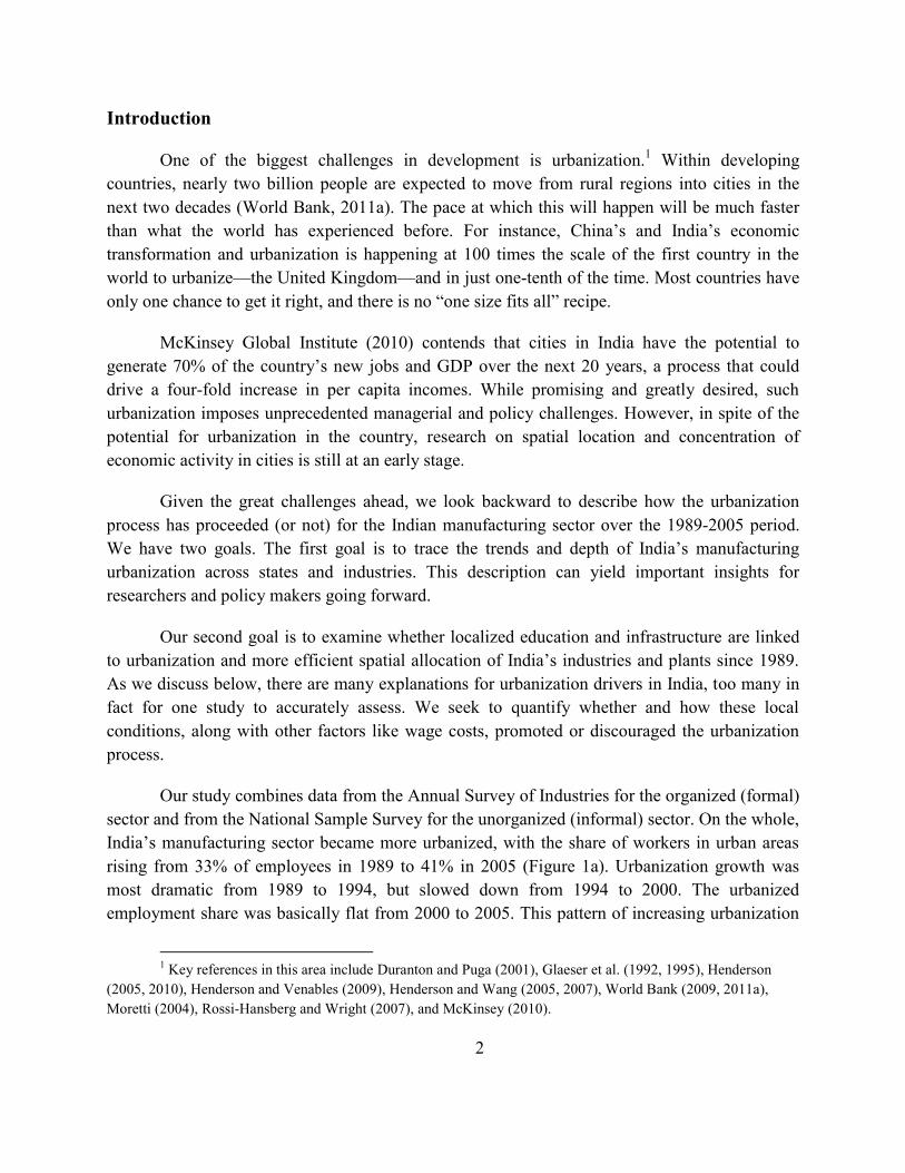
One of the biggest challenges in development is urbanization.1 Within developing countries, nearly two billion people are expected to move from rural regions into cities in the next two decades (World Bank, 2011a). The pace at which this will happen will be much faster than what the world has experienced before. For instance, China’s and India’s economic transformation and urbanization is happening at 100 times the scale of the first country in the world to urbanize—the United Kingdom—and in just one-tenth of the time. Most countries have only one chance to get it right, and there is no “one size fits all” recipe.

McKinsey Global Institute (2010) contends that cities in India have the potential to generate 70% of the country’s new jobs and GDP over the next 20 years, a process that could drive a four-fold increase in per capita incomes. While promising and greatly desired, such urbanization imposes unprecedented managerial and policy challenges. However, in spite of the potential for urbanization in the country, research on spatial location and concentration of economic activity in cities is still at an early stage.

Given the great challenges ahead, we look backward to describe how the urbanization process has proceeded (or not) for the Indian manufacturing sector over the 1989-2005 period. We have two goals. The first goal is to trace the trends and depth of India’s manufacturing urbanization across states and industries. This description can yield important insights for researchers and policy makers going forward.

Our second goal is to examine whether localized education and infrastructure are linked to urbanization and more efficient spatial allocation of India’s industries and plants since 1989. As we discuss below, there are many explanations for urbanization drivers in India, too many in fact for one study to accurately assess. We seek to quantify whether and how these local conditions, along with other factors like wage costs, promoted or discouraged the urbanization process.

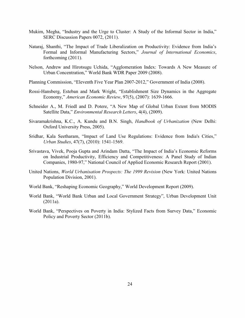
Our study combines data from the Annual Survey of Industries for the organized (formal) sector and from the National Sample Survey for the unorganized (informal) sector. On the whole, India’s manufacturing sector became more urbanized, with the share of workers in urban areas rising from 33% of employees in 1989 to 41% in 2005 (Figure 1a). Urbanization growth was most dramatic from 1989 to 1994, but slowed down from 1994 to 2000. The urbanized employment share was basically flat from 2000 to 2005. This pattern of increasing urbanization

1 Key references in this area include Duranton and Puga (2001), Glaeser et al. (1992, 1995), Henderson

(2005, 2010), Henderson and Venables (2009), Henderson and Wang (2005, 2007), World Bank (2009, 2011a), Moretti (2004), Rossi-Hansberg and Wright (2007), and McKinsey (2010).

3

was also present when looking just at manufacturing plant counts, but the opposite trend is observed for manufacturing output. The latter has increasingly moved towards rural areas. We investigate several features of these trends in detail.

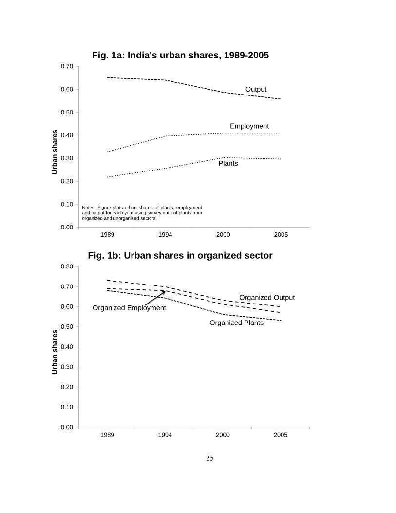
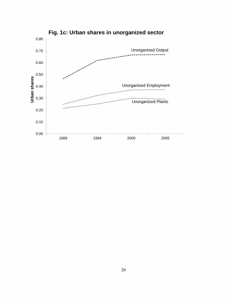
Our first investigation focuses on the relative movements of the organized and unorganized sectors. The differences, illustrated in Figures 1b and 1c, are striking. Throughout the 1989-2005 period, the organized sector moved from urban to rural locations, with its urban employment share declining from 69% in 1989 to 57% in 2005.2 On the other hand, urban employment share for the unorganized sector increased from 25% to 37%. Since the unorganized sector accounts for about 80% of employment in India’s manufacturing sector, the total urbanization level increased for the employment measure. Likewise, the organized sector accounts for over 80% of India’s output, so the aggregate output series instead becomes more rural. Section 2 examines the differences across states and industries within India. Simply put, the urbanization process and trends are very heterogeneous at the micro level.

To set the stage for our study of localized changes, Section 3 decomposes India’s overall urbanization changes into shifts in urbanization within districts versus changes in the spatial allocation of activity across districts. Using two decomposition techniques, we find that both within- and between-districts components are important and tend to work in the same direction for the urbanization of the unorganized sector and the de-urbanization of the organized sector. We show that the within-district component explains about three-quarters of the overall adjustments evident. Following this observation, we focus the rest of our paper on studying this within-district adjustment process.

To assess the factors contributing to these within-district shifts, we consider a series of regressions that quantify district traits that are associated with increased urbanization during this period. Per our second objective, we find substantial evidence that links greater urbanization to districts with more educated workforces and better infrastructure levels. Further, we find evidence that higher costs, or sharper differences in urban-rural cost levels, decrease the rate of urbanization. These effects are most pronounced in the unorganized sector and before 2000. We also use interaction regressions to show that industries with high capital and land intensity are more likely to locate in rural areas in districts with strong education and infrastructure levels.

By itself, there is no guarantee that the increased urbanization associated with education and infrastructure is optimal. Our final exercise is to construct simple spatial mismatch indices to test whether these urbanization trends are associated with more efficient allocation of industry

2 This movement of organized-sector plants and employment from urban to rural areas may explain some

of the findings of Cali and Menon (2009) regarding reduction in rural poverty. See also Foster and Rosenzweig (2003, 2004), Kundu (2002), and World Bank (2011b).

4

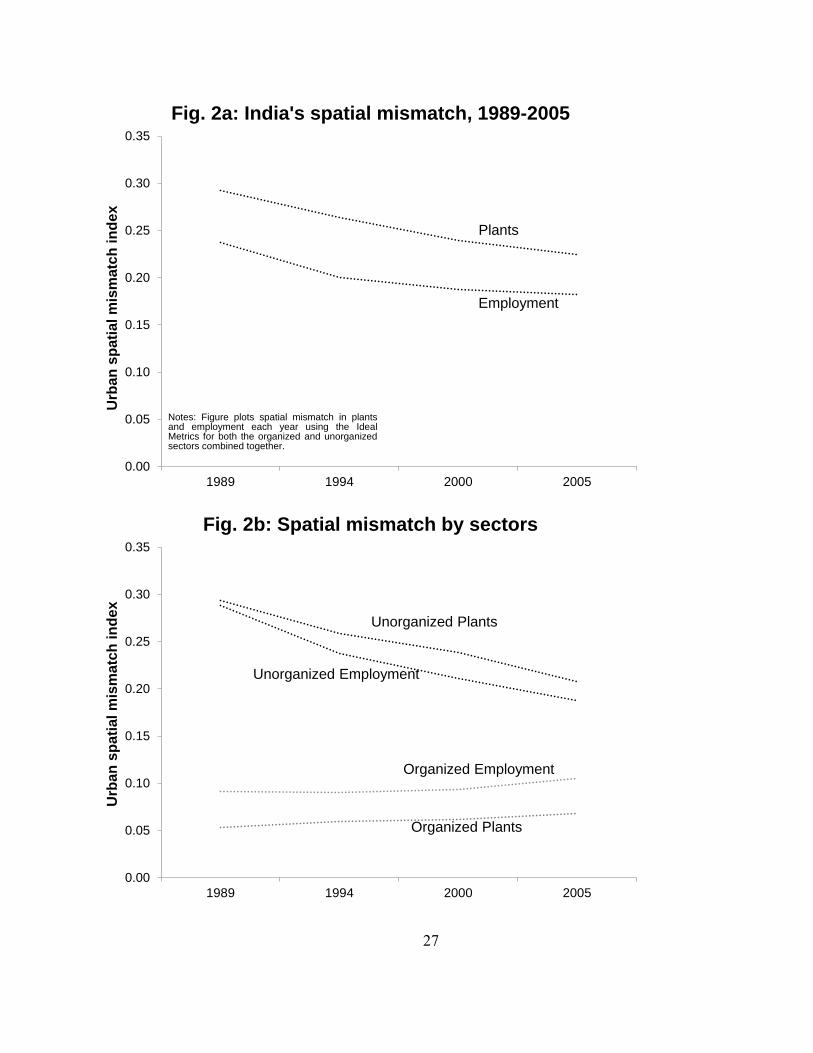
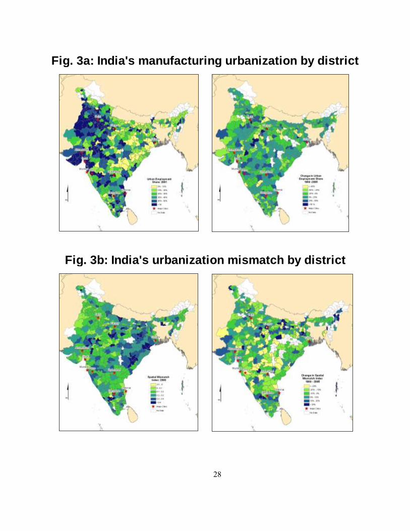
for districts between urban and rural settings. The spatial mismatch index compares the observed industry distribution of district employment across urban and rural locations to a counterfactual where plants or employment in the district are allocated (in some sense optimally) to urban and rural locations according to national propensities by industry to be in urban settings. As elaborated further below, higher mismatch values for a district indicate that plants that would have been expected to be in urban areas are in rural areas, and vice versa. Figures 2a-2b plot the trends in our spatial mismatch indices. Encouragingly, there has been an aggregate decline in spatial mismatch since 1989, primarily driven by improved allocation of the unorganized sector. Additional regressions identify that the urbanization shifts associated with better education and infrastructure have improved the spatial allocation of industry.

The plan of this paper is as follows. Section 2 discusses our data and the broad patterns of urbanization for India’s manufacturing sector. We also discuss in depth how urbanization is defined in India and issues for longitudinal consistency. Section 3 presents the decomposition of urbanization changes across districts. Section 4 considers the district-level traits associated with urbanization changes; this section also presents our interaction analysis of industry traits. Section 5 analyses spatial mismatch in industry allocations. The final section concludes and discusses implications from this work.

Section 2: Surveys of Indian Manufacturing--Organized and Unorganized Sectors

This paper employs cross-sectional establishment-level surveys of manufacturing enterprises carried out by the Government of India. Our work studies the manufacturing data from surveys conducted in fiscal years 1989, 1994, 2000, and 2005. In all four cases, the survey was undertaken over two fiscal years (e.g., the 1994 survey was conducted during 1994-1995), but we will only refer to the initial year for simplicity. This section describes some key features of these data for our study.3

It is important to first define and characterize the distinction between the organized and unorganized sectors in the Indian economy. These distinctions in the Indian context relate to establishment size. In manufacturing, the organized sector includes establishments with more than 10 workers if the establishment uses electricity. If the establishment does not use electricity, the threshold is 20 workers or more. These establishments are required to register under the India Factories Act of 1948. The unorganized manufacturing sector is, by default, composed of establishments which fall outside the scope of the Factories Act.

3 For additional detail on the manufacturing survey data, we refer the reader to Nataraj (2011), Kathuria et

al. (2010), Fernandes and Pakes (2008), Hasan and Jandoc (2010), and Ghani et al. (2011b). Dehejia and Panagariya (2010) provide a detailed overview of the services data and its important characteristics.

5

The organized manufacturing sector is surveyed by the Central Statistical Organization every year through the Annual Survey of Industries (ASI), while unorganized manufacturing establishments are separately surveyed by the National Sample Survey Organization (NSSO) at approximately five-year intervals. Establishments are surveyed with state and four-digit National Industry Classification (NIC) stratification. We use the provided sample weights to construct population-level estimates of total establishments and employment at the district and two-digit NIC level. We focus mostly on district and industry variation in our empirical analyses. Districts are administrative subdivisions of Indian states or union territories that are more appropriate spatial units for understanding the urbanization process.

These surveys identify for each establishment whether it is in an urban or rural location. Our study considers changes in urbanization over time, and thus the stability and comparability of this survey question over time are very important. To begin with, the statutory definition of an urban setting during our period of study is:

(a) All statutory places with a municipality, corporation, cantonment board or notified town area committee, etc., or

(b) A place satisfying the following three criteria simultaneously: i) A minimum population of 5,000; ii) At least 75% of male working population engaged in non-agricultural

pursuits; and iii) A density of population of at least 400 per sq. km. (1,000 per sq. mile).

This definition has been mostly stable since the 1961 Census. One set of adjustments with the 1971 and 1991 Censuses focused on including ‘outgrowths’ (e.g., railway colonies, university campuses, industrial townships, and residential and commercial complexes) that lay beyond strict town or village boundaries within a combined urban agglomeration concept for the purposes of classifications. A second set of adjustments enacted since the 1981 Census focused on the definition of the workforce and agricultural sector.4

Among our datasets, the 1989 survey follows the 1981 Census classification, the 1994 and 2000 surveys follow the 1991 classification, and the 2005 survey follows the 2001 Census classifications. Our primary focus is on urbanization changes since 1994, and the formal

4 India’s Ministry of Urban Development Report (2011), Kundu (2006, 2009, 2011a and 2011b), Himanshu

(2007), Mohan and Dasgupta (2005), Planning Commission (2008), Nelson and Uchida (2008), Bhagat (2011), Ghani (2010), Sivaramakrishna and Kundu (2005) provide greater details. Desmet et al. (2011) examine spatial development of India. Chrandrasekhar (2011) and Mohanan (2008) examine the trends in workers commuting between rural-urban areas.

6

definition of an urban area has not changed during this period. As we discuss further below, some sub-units of districts move from being rural areas to being urban areas with the 2001 Census compared to the 1991 Census when the sub-units begin to satisfy the urbanization criteria. This change can influence our measured urbanization levels, and we discuss below the robustness of our documented patterns to these reclassifications.5

It is important to note that India uses a more demanding set of criteria than most countries to define what is ‘urban’ (e.g., Bhagat, 2005; United Nations, 2001). For instance, substantial parts of U.S. metropolitan areas like Atlanta or Phoenix would be classified as rural in Indian statistical analyses because their population densities fall below 1000 persons per square mile. Thus, our measured urbanization for India will be lower than many international standards. This consideration does not affect, however, the longitudinal consistency of our trends for India.

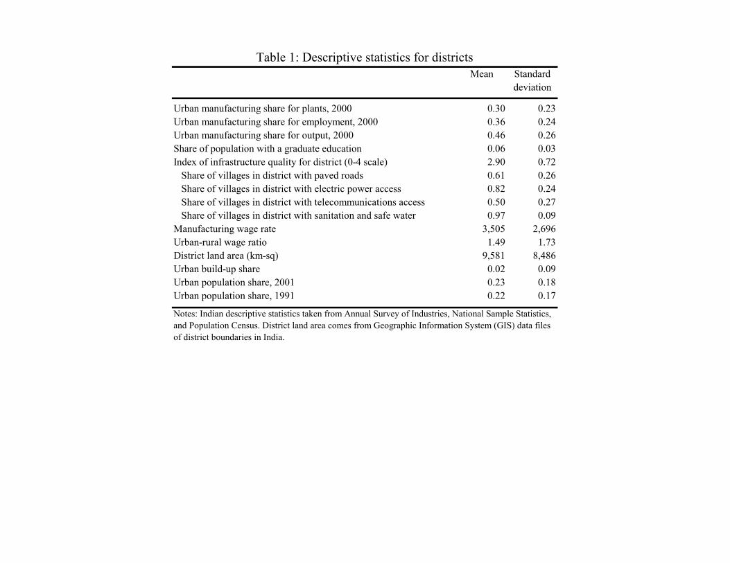
We primarily measure urbanization of manufacturing activity for a district through the share of manufacturing employment contained in establishments classified to be in an urban location. This choice most closely corresponds to the prior literature and the central concerns of Indian policy makers. We also consider urbanization of plant and outputs for comparison. Table 1 provides basic descriptive statistics on districts, further discussed below, that begin with the average of these measures for 2001.

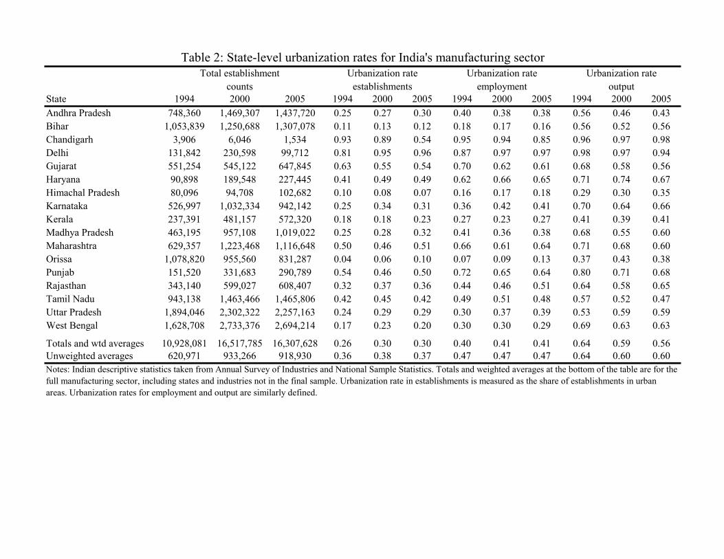
Table 2 lists the 17 major states from our sample and their urban shares, combining the organized and unorganized sectors. Figure 3a provides a graphical depiction. These states are a subset of India’s 35 states/union territories. Exclusions were due to three potential factors: 1) the state was not sampled across all of our surveys, 2) the small sample size for the state raised data quality concerns, or 3) persistent conflict and political turmoil existed in the region. We discuss below in greater detail the explicit criteria for a district’s inclusion in the regression sample. These exclusions are minor in terms of economic activity.

The most urbanized states in terms of manufacturing employment are Delhi and Chandigarh at over 90% in 2000, with Gujarat, Haryana, Maharashtra, and Punjab also above 60%. These states account roughly for 35% of urban employment and 47% of urban output for India in 2000, with these shares fairly stable over time. The larger states of Bihar, Orissa, Uttar Pradesh, and West Bengal have below-average urbanization rates. Bihar, Orissa, and Himachal Pradesh have urbanization rates of less than 20% for manufacturing employment.

5 Kundu (2011a) suggests that reclassification between the 1991 and 2001 Censuses is a minor factor.

Bhagat and Mohanty (2009) calculate that reclassifications account for about 12% of the total change in urbanization during the between the 1991 and 2001 Censuses.

7

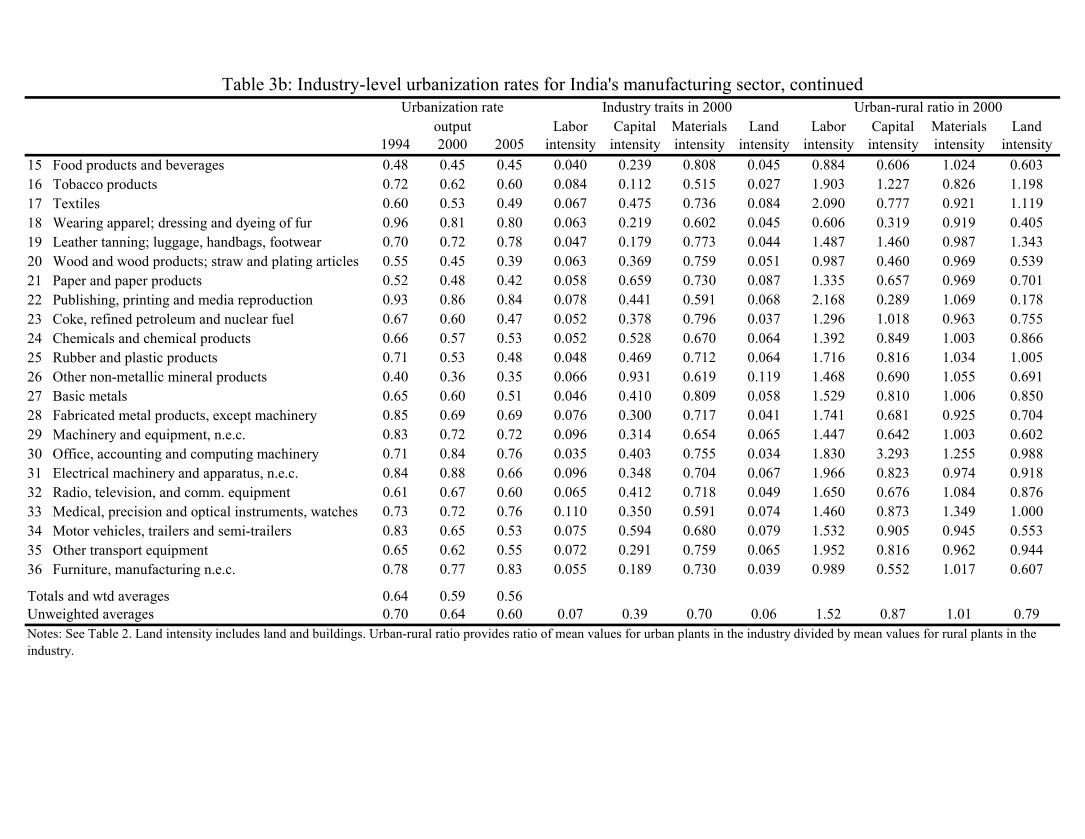
Tables 3a and 3b provide urban shares by two-digit NIC industry, again combining the organized and unorganized sectors. Office, accounting and computing machinery; Publishing, printing and media; and Medical, precision and optical instruments, watches are the most urbanized industries with greater than 80% of employment in urban plants. The least urbanized industries in 2000 are Wood and wood products; straw and plating articles; Other non-metallic mineral products; Tobacco products; and Food products and beverages, with under 30% of industry employment in an urban area. Major increases in urbanization of employment are evident for the Textiles; Leather tanning; luggage, handbags, footwear; Machinery and equipment, n.e.c.; and Office, accounting and computing machinery industries.

Table 3b presents some industry traits: 1) Labor intensity, defined as the total wage bill over value of shipments; 2) Capital intensity, defined as the total fixed capital value over value of shipments; 3) Materials intensity, defined as total raw materials costs over value of shipments; and 4) Land intensity, defined as the closing net land value over value of shipments. There is a 0.20 correlation between labor intensity and 2000 urbanization of employment across industries. There is a negative correlation of -0.05 for capital intensity. There is no correlation evident for the materials or land intensity.

The last part of Table 3b documents the observed ratio of these industry traits between urban and rural establishments for an industry. That is, the urban-rural labor intensity ratio measures the labor intensity of urban establishments to the labor intensity of rural establishments for each industry. The other ratios are similarly defined. Plants in urban areas generally employ more labor, similar levels of materials, and less capital and land than rural plants do. There is a 0.43 correlation between the urban-rural intensity difference and the urbanization rate for labor usage; the correlation to materials usage differentials is likewise high at 0.44. Capital intensity differentials are less correlated at 0.26, and land usage differentials are not correlated with overall urbanization levels.6

These descriptive tables refine one of the key trends noted in the introduction. Overall, manufacturing activity is becoming more urbanized as measured by employment and plants, while it is becoming less urbanized as measured by output. These trends are mainly explained by the share of organized and unorganized sectors for each metric and the differences in the urbanization trends for these sectors. The details in Tables 2-3b also show that urbanization increases are concentrated, rather than broad-based, even for employment. Only 8 of the 17 states and 7 of the 22 industries exhibit an increase in urbanization from 1994-2005. The

6 These metrics are developed using data for the year 2000 from the organized sector. We use the year 2000

to match our district traits taken from the 2001 Census described in Section 4. Several of these variables are not consistently available for unorganized sector. These correlations and our analyses below are robust to winsorizing these industry traits at their 5%/95% values.

8

remainder of the paper will analyze the traits of districts that have successfully urbanized over this period.7

Section 3: Decomposition of India’s Urban Share Changes

Table 4 presents our first district-level analysis. Following the productivity growth decomposition work of Baily et al. (1992), Griliches and Regev (1995), and Foster et al. (2001), we decompose the observed changes in the aggregate urbanization from 1994 to 2005 into the “within” changes in urban rates for districts (i.e., average growth in urbanization for districts weighted by initial employment shares) versus “between” changes across districts in activity (i.e., relocation of activity from districts with low initial urbanization rates to districts with high initial urbanization rates).

Let U denote the urbanization rate of India (in manufacturing employment) and Ud be the urbanization rate of district d. Sd is district d’s share of Indian manufacturing in employment. By definition, U = ∑d=1,...,D Sd∙Ud, where d indexes districts. Following Foster et al. (2001), our primary decomposition of changes from 1994 to 2005 takes the form:

ΔU94-05=∑d Sd,94∙ΔUd,94-05+∑d (Ud,94–U94)∙ΔSd,94-05+∑d ΔUd,94-05∙ΔSd,94-05, where the first term ∑d Sd,94∙ΔUd,94-05 is the within component that represents changes in urban shares within districts with districts weighted by initial employment shares for the Indian economy in 1994. Positive values indicate that districts tended to have increasing urban shares when weighted by initial employment.

The second term ∑d (Ud,94–U94)∙ΔSd,94-05 measures the between component which represents changes in employment shares across districts interacted with the initial deviation of districts from the national urban share. Positive values indicate employment tended to be reallocated towards districts that had higher initial urban shares.

The third term ∑d ΔUd,94-05∙ΔSd,94-05 is the covariance component that represents the interaction of changes in urban shares for districts across the period with changes in employment shares for districts across the period. Positive values indicate that fast-growing districts also experienced rising urban shares.

7 Ghani et al. (2011c) study the increase since 1994 in female-owned businesses in India. These

urbanization trends and the special role of the unorganized sector are not due to this increased role for women, as female-owned business shares track upwards in urban and rural settings together. See Dinkelman (2011) for the role of rural electricity in female employment ratios in South Africa.

9

These three components by definition sum to the total change in urban share in aggregate as well for each of the sectors in India. As we do not consider entry or exit of districts across years, our decomposition requires a balanced panel in Table 4. The urban shares in Panel A of Table 4 closely mirror the earlier trends. Table 4 provides the decomposition of urban shares in plants, employment, and output in aggregate manufacturing (columns 1-3), as well as across the organized and unorganized sectors.

Over the 1994 to 2005 period, the within- and between-district components generally operate in the same direction in Panel B. For the organized sector, both components serve to reduce the urbanization rate, while for the unorganized sector both components serve to increase the urbanization rate of plants and employment. The aggregate metrics follow the combination of these two in accordance to their relative shares. In almost every case, and especially for the organized sector, the within-district component is larger than the between-district component.

Interestingly, the covariance term is almost always negative for all three metrics of urbanization, suggesting that rapidly growing districts experienced relative declines in urbanization levels. Equivalently, this pattern suggests that urbanization growth was highest in districts that were growing their manufacturing base less than the national average. While the within- and between-district components tended to act in different directions for the organized and unorganized sectors, this covariance component was more consistent.

These patterns are confirmed in Panel C using the technique of Griliches and Regev (1995). This second technique and its merits/liabilities are outlined in greater detail by Foster et al. (2001). Most importantly, the technique lacks a covariance component, with this feature instead absorbed into both the within- and between-district components. Weighing against this disadvantage, the Griliches and Regev (1995) technique is more robust to measurement error. Using this technique provides very similar conclusions to those in Panel B. The appendix also shows that we obtain similar patterns when examining 1994-2000 and 2000-2005 separately.

These exercises set the stage for our regression analyses. The estimation techniques used in the remainder of the paper will thus mostly focus on changes in urbanization levels within district cells. These decompositions suggest that within-district changes capture the majority of the urbanization changes during this period. The Griliches and Regev (1995) technique provides the most straightforward calculation in this regard: the within-district component represents on average 83% of the total change observed. Using the Baily et al. (1992) technique and ignoring the covariance component, the within-district component accounts for about 75% of the total observed changes in absolute terms. Ongoing research is systematically evaluating the between-district component and the role of major transportation linkages (e.g., Lall et al. 2010).

10

Section 4: Empirical Analysis of Urban Movements in Economic Activity

This section analyzes the factors promoting or discouraging changes in urbanization from 1994 to 2005 in districts, with particular emphasis on education and infrastructure. We conduct our estimations at the district-industry level. In all regressions, we control for industry fixed effects to absorb changes in urbanization that are simply following national changes in urbanization levels for given industries. In other words, we will be considering factors that promote or discourage urbanization for a district beyond the change that would be expected based upon its industry composition. We first describe the district sample and the district traits that we consider, and then we present the estimation results.

District Sample

Our sample focuses on district-industry cells. Our core sample contains 262 districts out of a total district count for India of 630. This sizeable decline in district count is due to the steps taken to prepare a consistent estimation setting, with the primary decline being due to lack of information in the 2001 Census on the district’s traits (e.g., education, infrastructure). This Census information was only collected for about 400 districts.

In addition to our state-level restrictions noted earlier, our regression sample also requires that the district-industry be observed in all of our manufacturing surveys so that we can observe changes over time. Our explicit criteria with respect to district size are that the district has a population of at least one million in the 2001 Census and has 50 or more establishments sampled. Given our desire to study urbanization changes, we also exclude districts that had fewer than five urban plants or five rural plants. Finally, we exclude plants that have negative value add, which accounts for 6%-7% of employment.

These restrictions are not very significant in terms of economic activity. The resulting panel accounts for over 80% of plants, employment, and output in the manufacturing sector throughout the period of study. As important, the aggregate trends for these districts mirror that of India as a whole shown in the figures.

District Traits

Table 1 provides descriptive statistics on our districts. Beyond the starting urbanization level for a district-industry, our two most important explanatory variables are the education levels of the local labor force and the quality of local physical infrastructure. These two factors are consistently linked to India’s regional development.8 Education levels can play a central role in urbanization. Many local policy makers stress developing the human capital of their

8 For example, Lall (2007), Amin and Mattoo (2008), Mukim (2011), and Ghani et al. (2011a).

11

workforces, and India is no different (Amin and Mattoo, 2008). We measure the general education level of the district’s labor force from the 2001 Census as the percentage of adults with a graduate (post-secondary) degree. Our results below are robust to alternatively defining a district’s education as the percentage of adults with higher secondary education.

Our second trait is the physical infrastructure level of the district. Functioning urban areas depend critically on their underlying infrastructure. Infrastructure likewise connects urban and rural parts of a district. The government of India is providing substantial financial resources for infrastructure investment (Ministry of Urban Development, 2008). The 2001 Census provides figures on the number of villages in a district which have paved roads, electric power access, telecommunications access, and access to safe drinking water. We calculate the percentage of villages that have infrastructure access within a district and sum across the four measures to create a continuous composite metric of infrastructure which ranges from zero (no infrastructure access in any village) to four (full access to all four infrastructure components in all villages).9

We empirically assess the role of education and infrastructure for development without strong theoretical priors on their role, only noting their frequent emphasis by policy makers. We believe this agnostic approach is important as anecdotal accounts of India suggest multiple relationships are at play. For example, a natural baseline for education is that agglomeration economies or urbanization premiums are higher for skilled workers and industries. Observers note, however, that skilled workers may want to live outside of Indian cities to the extent that the amenities are lower in Indian cities than in the surrounding areas. Likewise, better infrastructure typically allows strong urbanization levels. However, cities in India often experience some of the largest infrastructure failures, and production of own electricity for organized sector firms is high in both settings. Thus better infrastructure capacity may allow establishments to move to rural locations.

Cost factors also play a critical role in location choice decisions for firms. We would ideally like to model several factors like rental prices, utilities prices, wage rates, and so on, but data on cost factors are very limited. We primarily focus on the wage rate of the district—examining both its average rate and the urban-rural ratio for a district. For a given district, we anticipate that both aspects can push firms to locate in rural areas. Lower average wages in a district may also attract plants searching for lower labor costs from neighboring districts.

District wage rates are calculated using firms in the organized sector in 2000. We focus on the organized sector as many firms in the unorganized sector do not report wages (and may

9 In six districts (major cities) which were not further subdivided into separate geographic units, these

indicators were not reported in the Census data. In these cases we assign the infrastructure access components as 100%. Our results are fully robust to excluding these major cities from the analysis sample.

12

not pay workers). To guard against outliers in the wage rates or ratios, we use the wage rate of the median employee in the district (and its urban and rural areas). We do not directly observe the full wage distribution, but instead calculate the metrics through plant averages and their relative employment levels. Wages are expressed in 2005 U.S. dollars. When discussing our results, we describe in greater detail the extent to which this factor may model other costs beyond labor factors for districts. We jointly model the average wage and urban-rural wage ratio variables as their correlation is small at 0.12.

Our remaining variables are covariates to contrast with the above factors. We first consider district land area. This metric is calculated by the World Bank using Geographic Information System (GIS) data files of district boundaries in India. Conditional on the other variables specified, we would not anticipate district scale playing an important role. Our focus is instead on the urban build-up of a district. Following Schneider et al. (2009), we consider the share of land in the district that is built-up for urban use. This fraction is calculated using 2001 MODIS satellite information at 500 meter spatial resolution. Built-up area, focusing on building structures, is a good proxy for urban area. Greater built-up area in a district can allow for stronger urbanization growth and is our best proxy for local land markets. A second proxy, termed land use intensity, is calculated as total land value of organized sector plants per unit of shipments.

For our core estimations, we do not model the overall level or change in population urbanization for a district, as this may be endogenous/follow the industry movements we consider. Robustness checks do consider, however, the change in population urbanization from the 1991 Census to the 2001 Census as a control. Thus, these regressions will be considering the movement of industry over-and-above that of the underlying population base. Section 2 noted that some sub-areas of districts change their urbanization status in 2001 and that this could affect our urbanization measures even if a plant’s location remained fixed. Including this change provides a quantitative check on whether this is important as the redefinition would apply to the sub-area’s population, too.

Basic District Analyses

Our base estimation for district d and industry i is specified as:

ΔUrban Shared,i = γ∙Initial Urban Shared,i + β∙Xd + ηi + ηs + εd,i.

The dependent variable, ΔUrban Shared,i, is the change in urban share in employment across a time period. Initial Urban Shared,i is the initial urban share in employment at the start of the period. This initial condition is important as we consider shares that are bounded. Thus, highly urbanized areas like Delhi have limited potential to further urbanize.

13

The vector Xd includes the district-level covariates defined above, and ηi is a vector of industry fixed effects. The industry fixed effects capture broad differences in production techniques and changes in urbanization levels that are specific to the period analyzed. We further include in some models a vector of state fixed effects ηs that capture heterogeneity in institutions, policies, and regulations across states. Including state fixed effects in our regression is non-trivial, as many education and infrastructure investments may be implemented at the state level. Nevertheless, we place greater confidence in results that are not sensitive to including the state fixed effects.

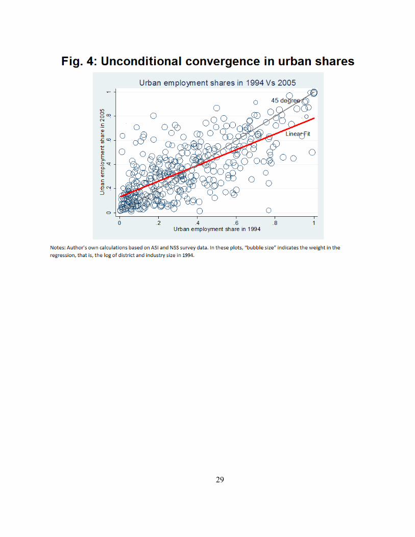
Table 5 investigates the correlates of India’s urbanization of employment at the district-industry level from 1994 to 2005. Estimations report standard errors clustered by district, have 1700 observations, and weight observations by the interaction of log district size and log industry size. The first row of Table 5 indicates strong conditional convergence, where higher initial urban shares for district-industries experience slower urbanization growth. Figure 4 provides a graphical depiction of unconditional convergence in urban shares. While this convergence is partly mechanical due to a share-based formulation, this property generally holds in other specification formats.

Columns 1 and 2 find that districts with better infrastructure and more educated workforces in 2000 experienced higher urbanization growth from 1994 to 2005. These patterns are evident with and without state fixed effects. In Columns 3 and 4, we include the two wage measures to model cost conditions in districts. Both measures are always negative and have t-statistics of at least 1.5. Without state fixed effects, the urban-rural differential tends to come through strongest, while the overall wage factor tends to come through strongest when state fixed effects are included. Either way, it is very clear that cost factors are important.

Columns 5 and 6 add district land area and change in urban population to the preceding specification. The latter is added as a robustness check to the issue of reclassification of rural areas highlighted in Section 2. These traits are not statistically important. The urban population change covariate has a large point estimate that disappears when including state fixed effects, perhaps indicative of growth differences across states. More important is the stability of the main regressors in these specifications.

Column 7 and 8 next control for the share of a district’s land area that is built-up for urban use.10 Our reported results use indicator variables to allow for non-linear effects in the

10 Some observers conclude that the combined effect of multiple layers of central, state, and municipal

regulations is producing an artificial urban land shortage in India. If true, this shortage results in urban land prices that are abnormally high in relation to India’s household income and alters the spatial structure of cities (Bertaud and Malpezzi 2001, 2003). Reductions in centrally located floor space and the potential to recycle land can push

14

built-up area shares. Higher build-up, especially in the top quartile, is strongly associated with increased urbanization; we find similar effects with other specification formats like linear shares. A plausible interpretation of these coefficients is that land availability is a strong governor of the urbanization process. While this interpretation would match anecdotal accounts of the constraints that land availability and real estate prices have for the location choices of manufacturing firms in India, this measure is indirect (e.g., compared to real estate price data) and thus caution in interpretation is warranted.

One effect of adding this control is that the coefficient on the infrastructure index declines somewhat and becomes insignificant when including state fixed effects. This is not too surprising given that the built-up metric in part captures higher infrastructure levels. Adding this variable, however, does not affect the results on our wage variables. We take from this set of results that cost factors that slow manufacturing urbanization in India are definitely present in the labor market and most likely present in the real estate market, too. The evidence further suggests that absolute cost levels and localized urban-rural cost ratios play a role in India’s urbanization.

Finally, Columns 9 and 10 alternatively model land use intensity by organized sector firms to measure the tightness of local land markets. Inclusion of this control does not affect our core variables. Interestingly, the coefficient is positive, suggesting greater urbanization is associated with tighter land markets. This counter-intuitive result is one factor suggesting caution regarding land availability variables.

Table 6a considers the robustness of these results over different time periods. The first two columns repeat the specifications in Columns 5 and 6 of Table 5 for 1994-2005. Columns 3 and 4 then consider 1994-2000, while Columns 5 and 6 consider 2000-2005. This disaggregation is interesting for several reasons. First, Figures 1a-1c showed the substantial flattening of the urbanization changes for 2000-2005 compared to 1994-2000, and it is interesting to identify what correlates with this slowdown. Second, as a basic robustness check on potential reclassification issues, the 1994-2000 change builds on a perfectly consistent urban-rural coding framework. Third, one might worry that measuring district traits in 2000-2001 is endogenous to changes occurring from 1994-2000, and so looking at the 2000-2005 period helps somewhat as these traits are then pre-determined (but still leaves open questions of omitted variable biases).

Most of the coefficients are similar to the 1994-2000 period in Columns 3 and 4, compared to the 1994-2005 baseline. The education variable loses some of its economic strength but remains very important statistically. The infrastructure measure loses some of its statistical strength but remains overall quite important, too. The most important difference is on the cost

urban development toward the periphery. This results in longer commuting trips and more challenging provision of urban infrastructure than would have been the case if land supply had been unconstrained.

15

side. Average wages have a positive and significant effect on urbanization when only industry fixed effects are controlled for. With state fixed effects, the average wage does not exhibit a strong relationship. By contrast, the urban-rural wage ratio is very important in explaining urbanization even after controlling for both industry and state fixed effects.

In Columns 5 and 6, we again find broad comparability for the 2000-2005 period. The education variable is especially strong, and the infrastructure variable is equivalent to the 1994-2000 estimations. The differences thus suggest that while the secular trend for India’s manufacturing urbanization has slowed, the localized importance of education and infrastructure has not. Among our cost measures, the average wage is negative and statistically significant. In contrast to the earlier period, the urban-rural wage differential is negative but not especially powerful in this second period.

These adjustments over time, especially in light of the aggregate trends, are interesting but we can only conjecture about the difference with respect to our cost variables. One plausible and intriguing possibility relates the series of economic reforms that India undertook in the 1980s and early 1990s. These reforms substantially impacted the manufacturing sector (e.g. Balakrishnan et al., 2000; Goldar and Kumari, 2003; Hashim et al., 2009; Srivastava et al. 2001). Prior to the reforms, many restrictions existed on where plants could locate. The early changes may have reflected a pent-up sorting to move to cheaper locations within districts. As this process worked itself out, general district wage rates became more important. We hope that future work can clarify the story behind this pattern.

Finally, Columns 7 and 8 of Table 6a present the correlates of changes in urban employment shares from 1989 to 2005. We focus primarily on the 1994-2005 period to maximize data quality and comparability; we also lose a quarter of the sample with the longer horizon. Nevertheless, the basic patterns we show are evident across the full time period, too.

Table 6b next compares our results on change in urban employment share from 1994 to 2005 with that observed in plants and output. Columns 3 and 4 show similar patterns when looking at the urbanization of plants, while the results with output urbanization are much weaker across the board. Only the growth in urbanization in districts with more educated workforces remains. Columns 7-10 show that these differences directly link to the differences between the organized and unorganized sectors.11 The unorganized sector, which accounts for most of plants and employment, mirrors the aggregate trends documented in Table 5. By contrast, changes in urban location decisions for the organized sector, which dominates output-based metrics, does not appear to be systematically linked to these metrics.

11 Observation counts decline in Columns 7-10 as we impose the minimum plant count restrictions for each

sector independently when separating their effects.

16

We find similar patterns—both for the aggregate employment measure and for differences across sectors—in a variety of robustness checks. To mention a few, our core estimations weight observations by an interaction of log district size and log industry size. This weighting strategy focuses attention on generally more important observations while avoiding biases that could be introduced with using actual placements. Nevertheless, we find similar results when weighting by actual employment or dropping the weights. We have also confirmed robustness of the education and infrastructure covariates to including other traits of districts like distance to a large city, household banking, demographic dividend, and import penetration. These do not affect our core patterns.

Our infrastructure index is a composite of four sub-components. Unreported regressions test introducing these four components separately. These estimations emphasize the importance of paved roads and electric power access. We are cautious about these disaggregated results, however, as the paved roads metric dominates in regressions that include state fixed effects, while the access to electric power metric dominates when state fixed effects are excluded. Given this sensitivity, we can only conclude that the aggregate infrastructure level is important. In a second test, we compared the combined sum of the infrastructure components to the minimum infrastructure level that exists for a district across these components (with and without the sanitation measure). The combined measure outperforms the minimum measure, suggesting that the overall package of infrastructure in a district matters more than the minimum level.

District-Industry Interaction Analyses

Results in Table 4-6b focus on district-level traits that explain where urbanization is occurring. These estimations control for industry differences but do not otherwise exploit industry-level variation. Table 7 evaluates the effect of interactions of industry traits with district characteristics on urbanization in plants, employment, and output across the three periods. Interacting industry and district traits can help us identify the characteristics of industries that are most sensitive to district features. Estimations control for district and industry fixed effects, so that the identification only comes through this interaction.

Panel A studies the effect of interaction of industry land intensity with education and infrastructure, while Panel B uses industry capital intensity instead. We focus on these two variables given their earlier emphasis. For education interactions, we tend to find little action. The point estimates are all negative, suggesting that land and capital intensive industries may be urbanizing less in districts with more educated workforces, but the results are not precisely estimated. On the other hand, we pick up more variation with the infrastructure interaction. Especially across the 1994-2000 period, land and capital intensive industries urbanized less in districts with better infrastructure. These results quantify a bit more precisely the correlations discussed earlier.

17

Besides capital and land intensity (and financial intensity which closely followed), unreported tests do not find other industry traits to be significant in interactions—either with the education and infrastructure measures, or with our cost-side wage factors. This limited response, suggesting that most of the district traits noted earlier acted similarly across industries, is surprising. Moreover, it raises some questions as to whether the urbanization changes improved the allocation of industry across India’s urban and rural regions. We turn to this in the next section.

Section 5: Urbanization and Spatial Mismatch

This section considers whether the above urbanization changes linked to better education and infrastructure also connected with a better allocation of industries between urban and rural settings for a district. Our depiction of spatial mismatch for establishments is simple and based upon the extent to which industries are nationally urbanized, as depicted in Table 3a. Industries like Office, accounting and computing machinery are predominantly in urban areas, while industries like Other non-metallic mineral products are predominantly rural.

We approach our spatial mismatch metrics as follows: Define the national urban share for an industry as National Urban%i. Taking a given district d, we identify the industry distribution of employment in the district that is in urban locations, combining both organized and unorganized sectors. Labeling this as Actual Urban Emp%d,i, our first calculation is

Actual Urban Allocationd = ∑i Actual Urban Emp%d,i∙National Urban%i,

This provides a weighted average of the extent to which industries located in urban positions in district d are typically urbanized nationally.

By itself, Actual Urban Allocationd is difficult to interpret, as districts have varying industrial compositions and urbanization levels. Our next step is then to create a comparison point for the district using the observed industry distribution of employment across both urban and rural settings. Conceptually, we ask what would have been the maximum allocation value possible if we assigned the urban employments to the industries in district d that are the most urbanized nationally. Imagine district d had an urban employment of 1000 workers. We would first take all employment from the Office, accounting and computing machinery industry and assign them to urban settings in the counterfactual. If this industry’s employment fell short of 1000 workers, we would then assign workers in the industry that is the second most urbanized nationally, and so on, until we have the industry distribution for the 1000 workers that should have been in the urban locations had industries sorted according to national trends. From this, we calculate

18

Ideal Urban Allocationd = ∑i Counterfactual Urban Emp%d,i∙National Urban%i.

By definition, this ideal metric will always equal or exceed the actual metric. Our primary measure of spatial mismatch is

Spatial Mismatchd = (Ideal Urban Allocationd – Actual Urban Allocationd ) / Ideal Allocationd

The index simply captures the degree to which the allocation of industries in a district does not conform to what we would have expected based upon national urbanization patterns.

Table 8 examines the spatial mismatch adjustments in a regression format very similar to Table 5. We control for the level of initial spatial mismatch for a district, always finding that areas with large initial spatial mismatch tend to decrease the mismatch over time. We also control for the change in urbanization evident during this period. We include this second control because spatial mismatch will be mechanically lower for more urbanized districts (at an extreme, no mismatch is possible if the district is 100% urbanized). The exact format of this control, or even its inclusion, is not important to our findings, but we include it to be conservative. It shows that our spatial mismatch metric declines as urbanization increases.

Among our focal variables, districts with more educated workforces show stronger declines in spatial mismatch. This is true in both sub-periods, and it is especially strong in the unorganized sector. In the organized sector, the education variable loses statistical significance once state fixed effects are controlled for. On the other hand, while the coefficient on the infrastructure measure is generally negative, it only displays a powerful connection during the 1994-2000 period. The cost factors do not appear important, beyond potentially what is captured by the base urban change variable.

These results are robust to several adjustments in metric design. We find similar results when normalizing by the average of Ideal Urban Allocationd and Actual Urban Allocationd and when considering the raw difference without normalization. We likewise find similar results when using measures of plant allocation without considering employment weights. Finally, we obtain similar results when not weighting the extent of misallocation by the national urbanization percentages for an industry but instead treating misallocation as a binary outcome.

This work is both encouraging and suggestive of future research. On one hand, while our metric design is admittedly simple, Table 8’s results suggest that the urbanization process in India linked to education, and perhaps infrastructure, is improving spatial industry allocation. Unreported estimations find these effects are most pronounced at medium and high levels of urbanization. On the other hand, changes in urban spatial allocations due to cost factors are not associated with improvements. This latter result could be due to limitations in our cost measures,

19

or it could suggest that the cost-based sorting does not help in this regard, which would be surprising. We hope that future research can clarify these matters.

We want to note that there are limits to our approach in the Indian context that should be considered in future work. Anecdotal accounts of India’s business suggest that some firms which should typically be in urban areas instead choose to locate in rural areas due to a combination of cheaper land prices, lower pollution restrictions and greater ability to generate own electricity, lower regulations, weaker congestion, and so on. Our approach does not allow for these types of realities, and it would be interesting in future work to attempt to model the ideal spatial allocation if these realities are considered.

Section 6: Conclusions and Implications

In this paper, we closely examine the movement of economic activity in Indian manufacturing between urban and rural areas. We find that while the organized sector is becoming less urbanized, the unorganized sector is becoming more urbanized. This process has been most closely linked to greater urbanization changes in districts with high education levels; a second role is often evident for public infrastructure as well. On the whole, these urbanization changes have modestly improved the urban-rural allocation of industries within India’s districts.

We want to note several key factors that our paper does not address. We have discussed at various points the limits on cost side factors. Especially with respect to real estate costs or limitations on land availability, our measures are quite crude. We hope that better data emerge in the future to refine these estimates. Related, anecdotal accounts for India suggest that urban-rural differences in regulation, severe congestion,12 and limits on urban property titles also direct firm location. While we have started to collect these data on the congestion side, this paper has not been able to model these factors systematically yet. Thus, to some extent, our wage variables may be capturing these issues as currently constructed.

Observers have frequently noted the relatively slow pace of India’s urbanization (even recognizing the differences in urban definitions); moreover, the movement of organized manufacturing sector plants to rural areas is surprising, given the relative youth of India’s manufacturing sector. Perceived wisdom is that this sluggishness is in part due to the limits imposed by India’s poor infrastructure and weaker education levels, among other factors like strict building regulations (Sridhar 2010). Our work supports these claims. Continued investment

12 Ministry of Urban Development (2008) finds that the problem of congestion does not come from the

number of vehicles in India but their concentration in a few selected cities, particularly in metropolitan cities. For instance, 32% of all vehicles are in metropolitan cities alone, and these cities constitute about 11% of the country’s total urban population.

20

in these factors, beyond their direct effects for Indian businesses, may also provide beneficial effects from an urbanization and spatial allocation perspective.13

Our findings suggest that policies that take an inclusionary approach to the urban informal economy may be more successful in promoting local development and managing its strains than those focused only on the formal sector. It is very important for Indian policy makers to recognize that much of the urbanization that is occurring is in the unorganized sector. Moreover, education and infrastructure investments, regardless of original motivation, are primarily operating through the unorganized sector. Going forward, adequate provision of infrastructure is necessary for the informal sector to develop. The more Indian cities recognize this influx and design appropriate policies and investments to support it, the more effective the policy interventions will be. Examples of inclusionary policies are mechanisms to ensure that urban informal livelihoods are integrated into urban plans, land allocation, and zoning regulations; that the urban informal workforce gains access to markets and to basic urban infrastructure services; and that organizations of informal workers participate in government procurement schemes and policy-making processes.

It is something of a paradox that India, among the most densely populated countries in the world, is also among the least urbanized. An important aspect for India’s continued growth is better and deeper urbanization over the next two decades than it has achieved over the past two decades.

References Amin, Mohammad and Aaditya Mattoo, “Human Capital and the Changing Structure of the

Indian Economy,” World Bank Policy Research Working Paper 4576 (2008).

Baily, Martin, Charles Hulten and David Campbell, “Productivity Dynamics in Manufacturing Plants,” Brookings Papers on Economic Activity: Microeconomics (1992): 187-249.

Balakrishnan, Pulapre, K. Pushpangadan and M. Suresh Babu, “Trade Liberalisation and Productivity Growth in Manufacturing: Evidence from Firm-level Panel Data,” Economic and Political Weekly, 35(41), (2000): 3679-3682.

13 Evaluating the impact of infrastructure investment on Russia’s peripheral regions, Brown et al. (2008)

find that the firm-level industrial data for 1989 and 2004 highlights a ‘death of distance.’ Particularly, regional infrastructure is found to be a critical driver of productivity for new and for privately-owned firms. Further, simulations of their model show that the benefits of infrastructure improvements are highest in regions where economic activity is already concentrated.

21

Bertaud, Alain and Stephen Malpezzi, “Measuring the Costs and Benefits of Urban Land Use Regulation: A Simple Model with an Application to Malaysia,” Journal of Housing Economics, 10(3), (2001): 393-418.

Bertaud, Alain and Stephen Malpezzi, “The Spatial Distribution of Population in 48 World Cities: Implications for Economies in Transition,” World Bank Working Paper (2003).

Bhagat, Ram, “Emerging Pattern of Urbanisation in India,” Economic and Political Weekly, 46(34), (2011): 10-12.

Bhagat, Ram and Soumya Mohanty, “Emerging Pattern of Urbanization and the Contribution of Migration in Urban Growth in India,” Asian Population Studies, 5(1), (2009): 5-20.

Bhagat, Ram, “Rural-Urban Classification and Municipal Governance in India,” Singapore Journal of Tropical Geography, 26(1), (2005): 61-73.

Brown, David, Marianne Fay, John Felkner, Somik Lall and Hyoung Gun Wang, “The Death of Distance? Economic Implications of Infrastructure Improvement in Russia,” EIB Papers, 13(2), (2008): 126-147.

Cali, Massimiliano and Carlo Menon, “Does Urbanisation Affect Rural (Chronic) Poverty? Evidence from Indian Districts,” SERC Working Paper 14 (2009).

Chandrasekhar, S., “Workers Commuting between the Rural and Urban: Estimates from NSSO Data,” Economic and Political Weekly, 46(46), (2011): 22-25.

Dehejia, Rajeev and Arvind Panagariya, “Services Growth in India: A Look Inside the Black Box,” Columbia Program on Indian Economic Policies Working Paper 2010-4 (2010).

Desmet, Klaus, Ejaz Ghani, Stephen O’Connell and Esteban Rossi-Hansberg, “The Spatial Development of India,” Working Paper (2011).

Dinkelman, Taryn, “The Effects of Rural Electrification on Employment: New Evidence from South Africa,” American Economic Review, 101(7), (2011): 3078-3108.

Duranton, Gilles, and Diego Puga, “Nursery Cities: Urban Diversity, Process Innovation, and the Life Cycle of Products,” American Economic Review, 91(5), (2001): 1454-1477.

Eaton, Jonathan, and Zvi Eckstein, “Cities and Growth: Theory and Evidence from France and Japan,” Regional Science and Urban Economics, 27(4-5), (1997): 443-474.

Fernandes, Ana, and Ariel Pakes, “Factor Utilization in Indian Manufacturing: A Look at the World Bank Investment Climate Survey Data,” NBER Working Paper 14178 (2008).

Foster, Andrew and Mark Rosenzweig, “Agricultural Productivity Growth, Rural Economic Diversity, and Economic Reforms: India, 1970-2000,” D. Gale Johnson Memorial Conference Paper (2003).

Foster, Andrew and Mark Rosenzweig, “Agricultural Development, Industrialization and Rural Inequality,” Working Paper (2004).

22

Foster, Lucia, John Haltiwanger and C.J. Krizan, “Aggregate Productivity Growth: Lessons from Microeconomic Evidence,” in Dean, Edward, Michael Harper and Charles Hulten (eds.) New Developments in Productivity Analysis (Chicago: University of Chicago Press, 2001): 303-372.

Ghani, Ejaz, “Do Cities Matter?” End Poverty in South Asia Blog, World Bank (2010).

Ghani, Ejaz, William Kerr and Stephen O'Connell, “Promoting Entrepreneurship, Growth, and Job Creation,” in Reshaping Tomorrow (Oxford, UK: Oxford University Press, 2011a).

Ghani, Ejaz, William Kerr and Stephen O'Connell, “Spatial Determinants of Entrepreneurship in India,” NBER Working Paper 17514 (2011b).

Ghani, Ejaz, William Kerr and Stephen O'Connell. “Local Industrial Structures and Female Entrepreneurship in India,” NBER Working Paper 17596 (2011c).

Griliches, Zvi and Haim Regev, “Productivity and Firm Turnover in Israeli Industry: 1979-1988,” Journal of Econometrics, 65, (1995): 175-203.

Glaeser, Edward, Jose Scheinkman and Andrei Shleifer, “Economic Growth in a Cross-Section of Cities,” Journal of Monetary Economics, 36(1), (1995): 117-143.

Glaeser, Edward, Hedi Kallal, Jose Scheinkman and Andrei. Shleifer, “Growth in Cities,” Journal of Political Economy, 100(6), (1992): 1126-1152.

Goldar, Bishwanath and Anita Kumari, “Import Liberalization and Productivity Growth in Indian Manufacturing Industries in the 1990s,” Developing Economies, 41(4), (2003): 436-60.

Hasan, Rana and Karl Jandoc, “The Distribution of Firm Size in India: What Can Survey Data Tell Us?” ADB Economics Working Paper 213 (2010).

Hashim, Danish, Ajay Kumar and Arvind Virmani, “Impact of Major Liberalization on Productivity: The J-Curve Hypothesis,” DEA Ministry of Finance Working Paper 5/2009, (2009).

Henderson, Vernon, “Cities and Development,” Journal of Regional Science, 50, (2010): 515-540.

Henderson, Vernon, “Urbanization and Growth,” in Aghion, Philippe and Steve Durlauf (eds.) Handbook of Economic Growth (Amsterdam: Elsevier, 2005): 1543-1591.

Henderson, Vernon and Anthony Venables, “Dynamics of City Formation,” Review of Economic Dynamics, 12(2), (2009): 233-254.

Henderson, Vernon and Hyoung Gun Wang, “Urbanization and City Growth: The Role of Institutions,” Regional Science and Urban Economics, 37(3), (2007): 283-313.

Henderson, Vernon and Hyoung Gun Wang, “Aspects of Rural-Urban Transformation of Countries,” Journal of Economic Geography, 5(1), (2005): 23-42.

23

Himanshu, “Recent Trends in Poverty and Inequality: Some Preliminary Results,” Economic and Political Weekly, 42(6), (2007): 497-508.

Kathuria, Vinish, Seethamma Natarajan, Rajesh Raj and Kunal Sen, “Organized versus Unorganized Manufacturing Performance in India in the Post-Reform Period,” MPRA Working Paper 20317 (2010).

Kundu, Amitabh, “Method in Madness: Urban Data from 2011 Census,” Economic and Political Weekly, 46(40), (2011a): 13-16.

Kundu, Amitabh, “Politics and Economics of Urban Growth,” Economic and Political Weekly, 42(20), (2011b): 10-12.

Kundu, Amitabh, “Exclusionary Urbanization in Asia: A Macro Overview,” Economic and Political Weekly, 44(48), (2009): 48-59.

Kundu, Amitabh, “Trends and Pattern of Urbanization and Their Economic Implications,” India Infrastructure Report (2006).

Kundu, Amitabh, Basanta Pradhan and A. Surmanium, “Dichotomy of Continuum: Analysis of Impact of Urban Centres on Their Periphery,” Economic and Political Weekly, 37(50), (2002): 5039-5046.

Lall, Somik, “Infrastructure and Regional Growth, Growth Dynamics and Policy Relevance for India,” The Annals of Regional Science, 41(3), (2007): 581-599.

Lall, Somik, Hyoung Wang, and Uwe Deichmann, “Infrastructure and City Competitiveness in India,” United Nations University Working Paper 2010/22 (2010).

McKinsey Global Institute, India’s Urban Awakening: Building New Cities, Sustaining Economic Growth (2010).

Ministry of Urban Development “Report on India Urban Infrastructure and Services,” High Powered Expert Committee for Estimating the Investment Requirements for Urban Infrastructure Services, Government of India (2011).

Ministry of Urban Development, “Study on Traffic and Transportation Policies and Strategies in Urban Areas in India,” Government of India Report (2008).

Mohan, Rakesh and Shubhagato Dasgupta, “The 21st Century: Asia Becomes Urban,” Economic and Political Weekly, 40(3), (2005): 213-223.

Mohanan, P.C., “Differentials in the Rural-Urban Movement of Workers,” The Journal of Income and Wealth, 30(1), (2008): 59-67.

Moretti, Enrico, “Human Capital Externalities in Cities,” in Henderson, J.V. and J.F. Thisse (eds.), Handbook of Regional and Urban Economics Volume 4 (Elsevier, 2004): 2243-2291.

24

Mukim, Megha, “Industry and the Urge to Cluster: A Study of the Informal Sector in India,” SERC Discussion Papers 0072, (2011).

Nataraj, Shanthi, “The Impact of Trade Liberalization on Productivity: Evidence from India’s Formal and Informal Manufacturing Sectors,” Journal of International Economics, forthcoming (2011).

Nelson, Andrew and Hirotsugu Uchida, “Agglomeration Index: Towards A New Measure of Urban Concentration,” World Bank WDR Paper 2009 (2008).

Planning Commission, “Eleventh Five Year Plan 2007-2012,” Government of India (2008).

Rossi-Hansberg, Esteban and Mark Wright, “Establishment Size Dynamics in the Aggregate Economy,” American Economic Review, 97(5), (2007): 1639-1666.

Schneider A., M. Friedl and D. Potere, “A New Map of Global Urban Extent from MODIS Satellite Data,” Environmental Research Letters, 4(4), (2009).

Sivaramakrishna, K.C., A. Kundu and B.N. Singh, Handbook of Urbanization (New Delhi: Oxford University Press, 2005).

Sridhar, Kala Seetharam, “Impact of Land Use Regulations: Evidence from India's Cities,” Urban Studies, 47(7), (2010): 1541-1569.

Srivastava, Vivek, Pooja Gupta and Arindam Datta, “The Impact of India’s Economic Reforms on Industrial Productivity, Efficiency and Competitiveness: A Panel Study of Indian Companies, 1980-97,” National Council of Applied Economic Research Report (2001).

United Nations, World Urbanisation Prospects: The 1999 Revision (New York: United Nations Population Division, 2001).

World Bank, “Reshaping Economic Geography,” World Development Report (2009).

World Bank, “World Bank Urban and Local Government Strategy”, Urban Development Unit (2011a).

World Bank, “Perspectives on Poverty in India: Stylized Facts from Survey Data,” Economic Policy and Poverty Sector (2011b).

25

0.00

0.10

0.20

0.30

0.40

0.50

0.60

0.70

1989 1994 2000 2005

Urb

an

sh

are

sFig. 1a: India's urban shares, 1989-2005

Plants

Output

Employment

Notes: Figure plots urban shares of plants, employmentand output for each year using survey data of plants fromorganized and unorganized sectors.

0.00

0.10

0.20

0.30

0.40

0.50

0.60

0.70

0.80

1989 1994 2000 2005

Urb

an

sh

are

s

Fig. 1b: Urban shares in organized sector

Organized Output

Organized Employment

Organized Plants

26

0.00

0.10

0.20

0.30

0.40

0.50

0.60

0.70

0.80

1989 1994 2000 2005

Urb

an

sh

are

sFig. 1c: Urban shares in unorganized sector

Unorganized Output

Unorganized Employment

Unorganized Plants

27

0.00

0.05

0.10

0.15

0.20

0.25

0.30

0.35

1989 1994 2000 2005

Urb

an

sp

ati

al

mis

matc

h i

nd

ex

Fig. 2a: India's spatial mismatch, 1989-2005

Plants

Employment

Notes: Figure plots spatial mismatch in plantsand employment each year using the IdealMetrics for both the organized and unorganizedsectors combined together.

0.00

0.05

0.10

0.15

0.20

0.25

0.30

0.35

1989 1994 2000 2005

Urb

an

sp

ati

al

mis

ma

tch

in

de

x

Fig. 2b: Spatial mismatch by sectors

Unorganized Employment

Unorganized Plants

Organized Employment

Organized Plants

28

Fig. 3a: India's manufacturing urbanization by district

Fig. 3b: India's urbanization mismatch by district

29

Mean Standarddeviation

Urban manufacturing share for plants, 2000 0.30 0.23Urban manufacturing share for employment, 2000 0.36 0.24Urban manufacturing share for output, 2000 0.46 0.26Share of population with a graduate education 0.06 0.03Index of infrastructure quality for district (0-4 scale) 2.90 0.72 Share of villages in district with paved roads 0.61 0.26 Share of villages in district with electric power access 0.82 0.24 Share of villages in district with telecommunications access 0.50 0.27 Share of villages in district with sanitation and safe water 0.97 0.09Manufacturing wage rate 3,505 2,696Urban-rural wage ratio 1.49 1.73District land area (km-sq) 9,581 8,486Urban build-up share 0.02 0.09Urban population share, 2001 0.23 0.18Urban population share, 1991 0.22 0.17

Table 1: Descriptive statistics for districts

Notes: Indian descriptive statistics taken from Annual Survey of Industries, National Sample Statistics, and Population Census. District land area comes from Geographic Information System (GIS) data files of district boundaries in India.

State 1994 2000 2005 1994 2000 2005 1994 2000 2005 1994 2000 2005Andhra Pradesh 748,360 1,469,307 1,437,720 0.25 0.27 0.30 0.40 0.38 0.38 0.56 0.46 0.43Bihar 1,053,839 1,250,688 1,307,078 0.11 0.13 0.12 0.18 0.17 0.16 0.56 0.52 0.56Chandigarh 3,906 6,046 1,534 0.93 0.89 0.54 0.95 0.94 0.85 0.96 0.97 0.98Delhi 131,842 230,598 99,712 0.81 0.95 0.96 0.87 0.97 0.97 0.98 0.97 0.94Gujarat 551,254 545,122 647,845 0.63 0.55 0.54 0.70 0.62 0.61 0.68 0.58 0.56Haryana 90,898 189,548 227,445 0.41 0.49 0.49 0.62 0.66 0.65 0.71 0.74 0.67Himachal Pradesh 80,096 94,708 102,682 0.10 0.08 0.07 0.16 0.17 0.18 0.29 0.30 0.35Karnataka 526,997 1,032,334 942,142 0.25 0.34 0.31 0.36 0.42 0.41 0.70 0.64 0.66Kerala 237,391 481,157 572,320 0.18 0.18 0.23 0.27 0.23 0.27 0.41 0.39 0.41Madhya Pradesh 463,195 957,108 1,019,022 0.25 0.28 0.32 0.41 0.36 0.38 0.68 0.55 0.60Maharashtra 629,357 1,223,468 1,116,648 0.50 0.46 0.51 0.66 0.61 0.64 0.71 0.68 0.60Orissa 1,078,820 955,560 831,287 0.04 0.06 0.10 0.07 0.09 0.13 0.37 0.43 0.38Punjab 151,520 331,683 290,789 0.54 0.46 0.50 0.72 0.65 0.64 0.80 0.71 0.68Rajasthan 343,140 599,027 608,407 0.32 0.37 0.36 0.44 0.46 0.51 0.64 0.58 0.65Tamil Nadu 943,138 1,463,466 1,465,806 0.42 0.45 0.42 0.49 0.51 0.48 0.57 0.52 0.47Uttar Pradesh 1,894,046 2,302,322 2,257,163 0.24 0.29 0.29 0.30 0.37 0.39 0.53 0.59 0.59West Bengal 1,628,708 2,733,376 2,694,214 0.17 0.23 0.20 0.30 0.30 0.29 0.69 0.63 0.63

Totals and wtd averages 10,928,081 16,517,785 16,307,628 0.26 0.30 0.30 0.40 0.41 0.41 0.64 0.59 0.56Unweighted averages 620,971 933,266 918,930 0.36 0.38 0.37 0.47 0.47 0.47 0.64 0.60 0.60

Table 2: State-level urbanization rates for India's manufacturing sector

Notes: Indian descriptive statistics taken from Annual Survey of Industries and National Sample Statistics. Totals and weighted averages at the bottom of the table are for the full manufacturing sector, including states and industries not in the final sample. Urbanization rate in establishments is measured as the share of establishments in urban areas. Urbanization rates for employment and output are similarly defined.

Total establishment Urbanization rate Urbanization rate Urbanization ratecounts establishments employment output

1994 2000 2005 1994 2000 2005 1994 2000 200515 Food products and beverages 2,391,234 2,962,970 2,572,043 0.19 0.22 0.20 0.24 0.27 0.2516 Tobacco products 1,004,510 2,062,543 2,753,644 0.20 0.22 0.17 0.32 0.28 0.2417 Textiles 1,971,821 2,239,348 2,312,117 0.24 0.31 0.32 0.37 0.42 0.4518 Wearing apparel; dressing and dyeing of fur 90,952 2,785,199 3,158,538 0.67 0.40 0.40 0.85 0.52 0.5219 Leather tanning; luggage, handbags, footwear 190,786 171,759 144,328 0.44 0.49 0.74 0.63 0.68 0.8020 Wood and wood products; straw and plating articles 1,957,120 2,720,752 1,895,690 0.15 0.13 0.11 0.20 0.16 0.1521 Paper and paper products 63,172 90,214 165,652 0.59 0.70 0.38 0.60 0.66 0.4722 Publishing, printing and media reproduction 105,479 144,293 116,764 0.76 0.84 0.86 0.84 0.88 0.8723 Coke, refined petroleum and nuclear fuel 5,075 7,429 6,435 0.48 0.27 0.20 0.48 0.43 0.3424 Chemicals and chemical products 98,048 216,410 401,055 0.44 0.51 0.29 0.60 0.53 0.4225 Rubber and plastic products 74,771 95,352 74,108 0.76 0.65 0.67 0.81 0.69 0.6126 Other non-metallic mineral products 686,560 784,551 606,049 0.15 0.16 0.17 0.22 0.22 0.2227 Basic metals 38,086 43,127 39,461 0.80 0.65 0.62 0.74 0.70 0.5728 Fabricated metal products, except machinery 422,420 640,256 616,937 0.44 0.43 0.41 0.64 0.61 0.6029 Machinery and equipment, n.e.c. 319,227 171,138 178,220 0.33 0.53 0.61 0.63 0.73 0.7630 Office, accounting and computing machinery 498 303 931 0.95 0.94 0.91 0.77 0.88 0.8631 Electrical machinery and apparatus, n.e.c. 29,495 67,896 112,788 0.67 0.66 0.54 0.83 0.79 0.6632 Radio, television, and comm. equipment 7,355 7,589 5,863 0.75 0.84 0.71 0.76 0.79 0.7033 Medical, precision and optical instruments, watches 11,715 9,190 10,283 0.96 0.82 0.85 0.82 0.80 0.7734 Motor vehicles, trailers and semi-trailers 6,924 24,186 16,664 0.65 0.84 0.63 0.84 0.77 0.6035 Other transport equipment 22,955 17,495 26,002 0.76 0.70 0.78 0.82 0.77 0.7636 Furniture, manufacturing n.e.c. 1,429,878 1,255,784 1,094,058 0.38 0.54 0.54 0.47 0.60 0.62

Totals and wtd averages 10,928,081 16,517,785 16,307,628 0.26 0.30 0.30 0.40 0.41 0.41Unweighted averages 496,731 750,808 741,256 0.52 0.53 0.50 0.60 0.59 0.55

Table 3a: Industry-level urbanization rates for India's manufacturing sector

Notes: See Table 2.

Total establishment Urbanization rate Urbanization ratecounts establishments employment

Labor Capital Materials Land Labor Capital Materials Land1994 2000 2005 intensity intensity intensity intensity intensity intensity intensity intensity

15 Food products and beverages 0.48 0.45 0.45 0.040 0.239 0.808 0.045 0.884 0.606 1.024 0.60316 Tobacco products 0.72 0.62 0.60 0.084 0.112 0.515 0.027 1.903 1.227 0.826 1.19817 Textiles 0.60 0.53 0.49 0.067 0.475 0.736 0.084 2.090 0.777 0.921 1.11918 Wearing apparel; dressing and dyeing of fur 0.96 0.81 0.80 0.063 0.219 0.602 0.045 0.606 0.319 0.919 0.40519 Leather tanning; luggage, handbags, footwear 0.70 0.72 0.78 0.047 0.179 0.773 0.044 1.487 1.460 0.987 1.34320 Wood and wood products; straw and plating articles 0.55 0.45 0.39 0.063 0.369 0.759 0.051 0.987 0.460 0.969 0.53921 Paper and paper products 0.52 0.48 0.42 0.058 0.659 0.730 0.087 1.335 0.657 0.969 0.70122 Publishing, printing and media reproduction 0.93 0.86 0.84 0.078 0.441 0.591 0.068 2.168 0.289 1.069 0.17823 Coke, refined petroleum and nuclear fuel 0.67 0.60 0.47 0.052 0.378 0.796 0.037 1.296 1.018 0.963 0.75524 Chemicals and chemical products 0.66 0.57 0.53 0.052 0.528 0.670 0.064 1.392 0.849 1.003 0.86625 Rubber and plastic products 0.71 0.53 0.48 0.048 0.469 0.712 0.064 1.716 0.816 1.034 1.00526 Other non-metallic mineral products 0.40 0.36 0.35 0.066 0.931 0.619 0.119 1.468 0.690 1.055 0.69127 Basic metals 0.65 0.60 0.51 0.046 0.410 0.809 0.058 1.529 0.810 1.006 0.85028 Fabricated metal products, except machinery 0.85 0.69 0.69 0.076 0.300 0.717 0.041 1.741 0.681 0.925 0.70429 Machinery and equipment, n.e.c. 0.83 0.72 0.72 0.096 0.314 0.654 0.065 1.447 0.642 1.003 0.60230 Office, accounting and computing machinery 0.71 0.84 0.76 0.035 0.403 0.755 0.034 1.830 3.293 1.255 0.98831 Electrical machinery and apparatus, n.e.c. 0.84 0.88 0.66 0.096 0.348 0.704 0.067 1.966 0.823 0.974 0.91832 Radio, television, and comm. equipment 0.61 0.67 0.60 0.065 0.412 0.718 0.049 1.650 0.676 1.084 0.87633 Medical, precision and optical instruments, watches 0.73 0.72 0.76 0.110 0.350 0.591 0.074 1.460 0.873 1.349 1.00034 Motor vehicles, trailers and semi-trailers 0.83 0.65 0.53 0.075 0.594 0.680 0.079 1.532 0.905 0.945 0.55335 Other transport equipment 0.65 0.62 0.55 0.072 0.291 0.759 0.065 1.952 0.816 0.962 0.94436 Furniture, manufacturing n.e.c. 0.78 0.77 0.83 0.055 0.189 0.730 0.039 0.989 0.552 1.017 0.607

Totals and wtd averages 0.64 0.59 0.56Unweighted averages 0.70 0.64 0.60 0.07 0.39 0.70 0.06 1.52 0.87 1.01 0.79

Urbanization rateoutput

Urban-rural ratio in 2000Industry traits in 2000

Notes: See Table 2. Land intensity includes land and buildings. Urban-rural ratio provides ratio of mean values for urban plants in the industry divided by mean values for rural plants in the industry.

Table 3b: Industry-level urbanization rates for India's manufacturing sector, continued

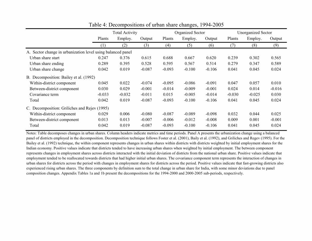
Plants Employ. Output Plants Employ. Output Plants Employ. Output(1) (2) (3) (4) (5) (6) (7) (8) (9)

Urban share start 0.247 0.376 0.615 0.688 0.667 0.620 0.239 0.302 0.565 Urban share ending 0.289 0.395 0.528 0.595 0.567 0.514 0.279 0.347 0.589 Urban share change 0.042 0.019 -0.087 -0.093 -0.100 -0.106 0.041 0.045 0.024

Within-district component 0.045 0.022 -0.074 -0.095 -0.086 -0.091 0.047 0.057 0.010 Between-district component 0.030 0.029 -0.001 -0.014 -0.009 -0.001 0.024 0.014 -0.016 Covariance term -0.033 -0.032 -0.011 0.015 -0.005 -0.014 -0.030 -0.025 0.030 Total 0.042 0.019 -0.087 -0.093 -0.100 -0.106 0.041 0.045 0.024

Within-district component 0.029 0.006 -0.080 -0.087 -0.089 -0.098 0.032 0.044 0.025 Between-district component 0.013 0.013 -0.007 -0.006 -0.012 -0.008 0.009 0.001 -0.001 Total 0.042 0.019 -0.087 -0.093 -0.100 -0.106 0.041 0.045 0.024

C. Decomposition: Griliches and Rejev (1995)

Notes: Table decomposes changes in urban shares. Column headers indicate metrics and time periods. Panel A presents the urbanization change using a balanced panel of districts employed in the decomposition. Decomposition technique follows Foster et al. (2001), Baily et al. (1992), and Griliches and Regev (1995). For the Bailey et al. (1992) technique, the within component represents changes in urban shares within districts with districts weighted by initial employment shares for the Indian economy. Positive values indicate that districts tended to have increasing urban shares when weighted by initial employment. The between component represents changes in employment shares across districts interacted with the initial deviation of districts from the national urban share. Positive values indicate that employment tended to be reallocated towards districts that had higher initial urban shares. The covariance component term represents the interaction of changes in urban shares for districts across the period with changes in employment shares for districts across the period. Positive values indicate that fast-growing districts also experienced rising urban shares. The three components by definition sum to the total change in urban share for India, with some minor deviations due to panel composition changes. Appendix Tables 1a and 1b present the decompositions for the 1994-2000 and 2000-2005 sub-periods, respectively.

Table 4: Decompositions of urban share changes, 1994-2005Total Activity Organized Sector Unorganized Sector

A. Sector change in urbanization level using balanced panel

B. Decomposition: Bailey et al. (1992)

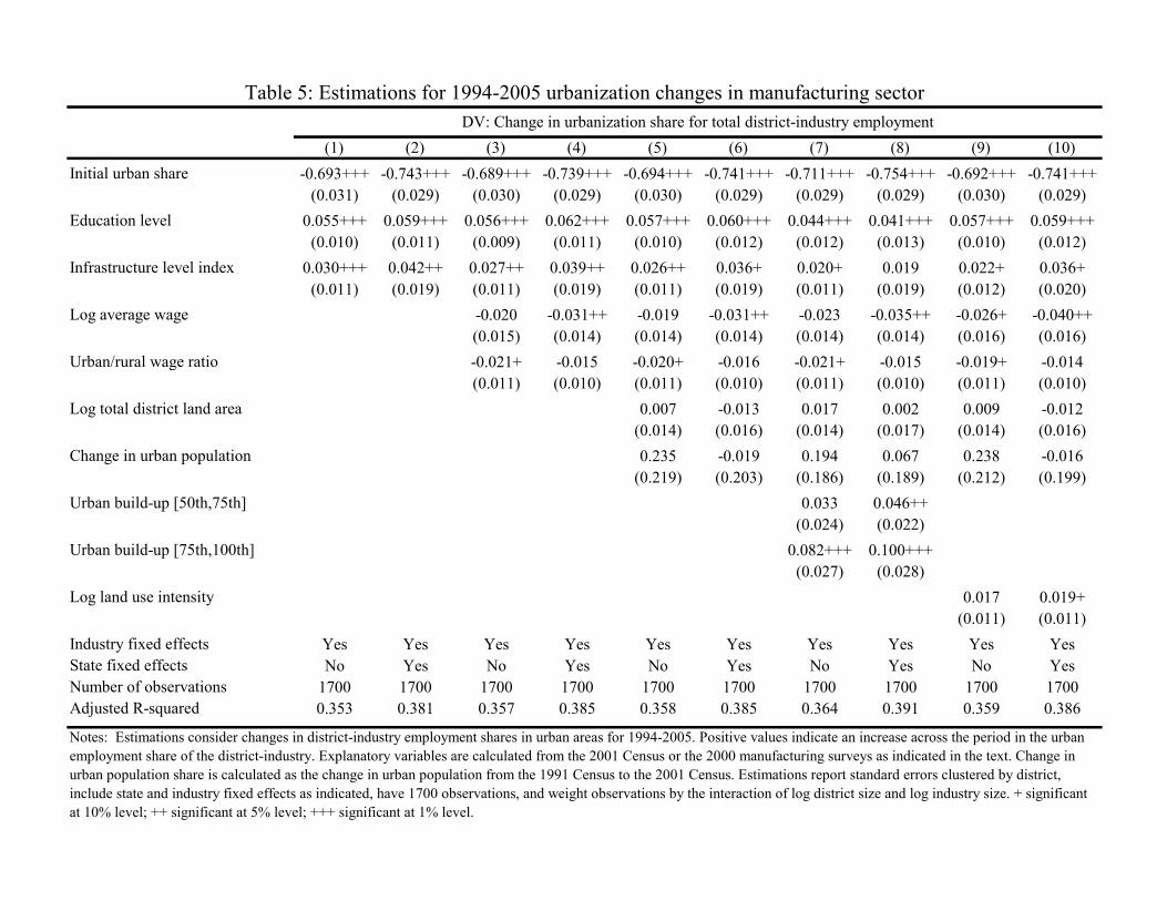
(1) (2) (3) (4) (5) (6) (7) (8) (9) (10)Initial urban share -0.693+++ -0.743+++ -0.689+++ -0.739+++ -0.694+++ -0.741+++ -0.711+++ -0.754+++ -0.692+++ -0.741+++

(0.031) (0.029) (0.030) (0.029) (0.030) (0.029) (0.029) (0.029) (0.030) (0.029)Education level 0.055+++ 0.059+++ 0.056+++ 0.062+++ 0.057+++ 0.060+++ 0.044+++ 0.041+++ 0.057+++ 0.059+++

(0.010) (0.011) (0.009) (0.011) (0.010) (0.012) (0.012) (0.013) (0.010) (0.012)Infrastructure level index 0.030+++ 0.042++ 0.027++ 0.039++ 0.026++ 0.036+ 0.020+ 0.019 0.022+ 0.036+

(0.011) (0.019) (0.011) (0.019) (0.011) (0.019) (0.011) (0.019) (0.012) (0.020)Log average wage -0.020 -0.031++ -0.019 -0.031++ -0.023 -0.035++ -0.026+ -0.040++

(0.015) (0.014) (0.014) (0.014) (0.014) (0.014) (0.016) (0.016)Urban/rural wage ratio -0.021+ -0.015 -0.020+ -0.016 -0.021+ -0.015 -0.019+ -0.014

(0.011) (0.010) (0.011) (0.010) (0.011) (0.010) (0.011) (0.010)Log total district land area 0.007 -0.013 0.017 0.002 0.009 -0.012

(0.014) (0.016) (0.014) (0.017) (0.014) (0.016)Change in urban population 0.235 -0.019 0.194 0.067 0.238 -0.016

(0.219) (0.203) (0.186) (0.189) (0.212) (0.199)Urban build-up [50th,75th] 0.033 0.046++

(0.024) (0.022)Urban build-up [75th,100th] 0.082+++ 0.100+++

(0.027) (0.028)Log land use intensity 0.017 0.019+

(0.011) (0.011)Industry fixed effects Yes Yes Yes Yes Yes Yes Yes Yes Yes YesState fixed effects No Yes No Yes No Yes No Yes No YesNumber of observations 1700 1700 1700 1700 1700 1700 1700 1700 1700 1700Adjusted R-squared 0.353 0.381 0.357 0.385 0.358 0.385 0.364 0.391 0.359 0.386

Table 5: Estimations for 1994-2005 urbanization changes in manufacturing sectorDV: Change in urbanization share for total district-industry employment

Notes: Estimations consider changes in district-industry employment shares in urban areas for 1994-2005. Positive values indicate an increase across the period in the urban employment share of the district-industry. Explanatory variables are calculated from the 2001 Census or the 2000 manufacturing surveys as indicated in the text. Change in urban population share is calculated as the change in urban population from the 1991 Census to the 2001 Census. Estimations report standard errors clustered by district, include state and industry fixed effects as indicated, have 1700 observations, and weight observations by the interaction of log district size and log industry size. + significant at 10% level; ++ significant at 5% level; +++ significant at 1% level.

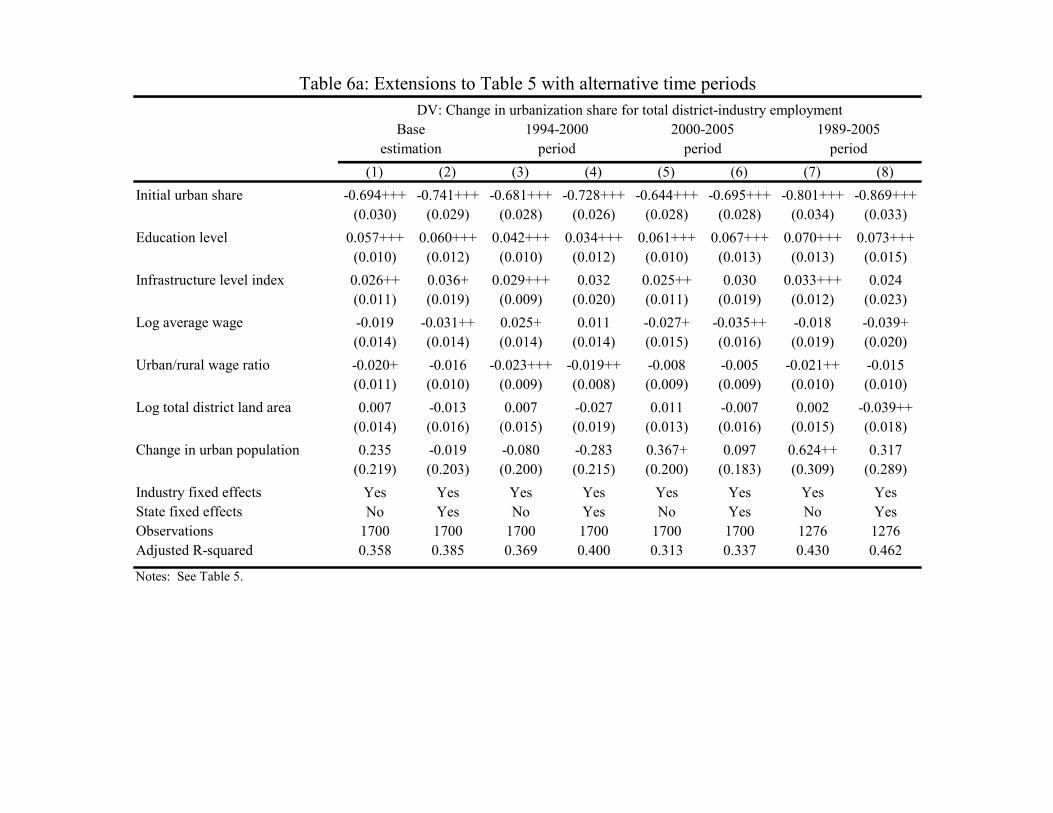
(1) (2) (3) (4) (5) (6) (7) (8)Initial urban share -0.694+++ -0.741+++ -0.681+++ -0.728+++ -0.644+++ -0.695+++ -0.801+++ -0.869+++

(0.030) (0.029) (0.028) (0.026) (0.028) (0.028) (0.034) (0.033)Education level 0.057+++ 0.060+++ 0.042+++ 0.034+++ 0.061+++ 0.067+++ 0.070+++ 0.073+++

(0.010) (0.012) (0.010) (0.012) (0.010) (0.013) (0.013) (0.015)Infrastructure level index 0.026++ 0.036+ 0.029+++ 0.032 0.025++ 0.030 0.033+++ 0.024

(0.011) (0.019) (0.009) (0.020) (0.011) (0.019) (0.012) (0.023)Log average wage -0.019 -0.031++ 0.025+ 0.011 -0.027+ -0.035++ -0.018 -0.039+

(0.014) (0.014) (0.014) (0.014) (0.015) (0.016) (0.019) (0.020)Urban/rural wage ratio -0.020+ -0.016 -0.023+++ -0.019++ -0.008 -0.005 -0.021++ -0.015

(0.011) (0.010) (0.009) (0.008) (0.009) (0.009) (0.010) (0.010)Log total district land area 0.007 -0.013 0.007 -0.027 0.011 -0.007 0.002 -0.039++

(0.014) (0.016) (0.015) (0.019) (0.013) (0.016) (0.015) (0.018)Change in urban population 0.235 -0.019 -0.080 -0.283 0.367+ 0.097 0.624++ 0.317

(0.219) (0.203) (0.200) (0.215) (0.200) (0.183) (0.309) (0.289)Industry fixed effects Yes Yes Yes Yes Yes Yes Yes YesState fixed effects No Yes No Yes No Yes No YesObservations 1700 1700 1700 1700 1700 1700 1276 1276Adjusted R-squared 0.358 0.385 0.369 0.400 0.313 0.337 0.430 0.462

Table 6a: Extensions to Table 5 with alternative time periods

Notes: See Table 5.

DV: Change in urbanization share for total district-industry employmentBase

estimation1994-2000

period2000-2005

period1989-2005

period

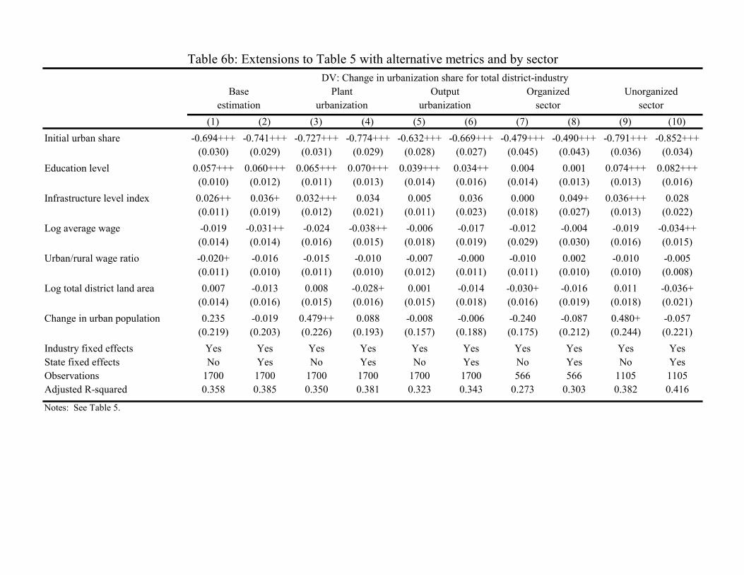
(1) (2) (3) (4) (5) (6) (7) (8) (9) (10)Initial urban share -0.694+++ -0.741+++ -0.727+++ -0.774+++ -0.632+++ -0.669+++ -0.479+++ -0.490+++ -0.791+++ -0.852+++

(0.030) (0.029) (0.031) (0.029) (0.028) (0.027) (0.045) (0.043) (0.036) (0.034)Education level 0.057+++ 0.060+++ 0.065+++ 0.070+++ 0.039+++ 0.034++ 0.004 0.001 0.074+++ 0.082+++

(0.010) (0.012) (0.011) (0.013) (0.014) (0.016) (0.014) (0.013) (0.013) (0.016)Infrastructure level index 0.026++ 0.036+ 0.032+++ 0.034 0.005 0.036 0.000 0.049+ 0.036+++ 0.028

(0.011) (0.019) (0.012) (0.021) (0.011) (0.023) (0.018) (0.027) (0.013) (0.022)Log average wage -0.019 -0.031++ -0.024 -0.038++ -0.006 -0.017 -0.012 -0.004 -0.019 -0.034++

(0.014) (0.014) (0.016) (0.015) (0.018) (0.019) (0.029) (0.030) (0.016) (0.015)Urban/rural wage ratio -0.020+ -0.016 -0.015 -0.010 -0.007 -0.000 -0.010 0.002 -0.010 -0.005

(0.011) (0.010) (0.011) (0.010) (0.012) (0.011) (0.011) (0.010) (0.010) (0.008)Log total district land area 0.007 -0.013 0.008 -0.028+ 0.001 -0.014 -0.030+ -0.016 0.011 -0.036+

(0.014) (0.016) (0.015) (0.016) (0.015) (0.018) (0.016) (0.019) (0.018) (0.021)Change in urban population 0.235 -0.019 0.479++ 0.088 -0.008 -0.006 -0.240 -0.087 0.480+ -0.057

(0.219) (0.203) (0.226) (0.193) (0.157) (0.188) (0.175) (0.212) (0.244) (0.221)Industry fixed effects Yes Yes Yes Yes Yes Yes Yes Yes Yes YesState fixed effects No Yes No Yes No Yes No Yes No YesObservations 1700 1700 1700 1700 1700 1700 566 566 1105 1105Adjusted R-squared 0.358 0.385 0.350 0.381 0.323 0.343 0.273 0.303 0.382 0.416

estimation urbanization urbanization sector sector

Notes: See Table 5.

Table 6b: Extensions to Table 5 with alternative metrics and by sectorDV: Change in urbanization share for total district-industry

Base Plant Output Organized Unorganized

1994-2005 1994-2000 2000-2005 1994-2005 1994-2000 2000-2005 1994-2005 1994-2000 2000-2005(1) (2) (3) (4) (5) (6) (7) (8) (9)

Initial urban share -0.824+++ -0.840+++ -0.777+++ -0.811+++ -0.811+++ -0.739+++ -0.730+++ -0.814+++ -0.761+++(0.033) (0.031) (0.032) (0.034) (0.030) (0.035) (0.031) (0.029) (0.031)

Education level x -0.021 -0.026+ -0.015 -0.026 -0.020 -0.018 -0.028 -0.007 -0.019 Industry land intensity (0.019) (0.015) (0.019) (0.018) (0.014) (0.019) (0.023) (0.019) (0.023)Infrastructure level index x -0.036++ -0.042+++ -0.030+ -0.022 -0.039+++ -0.016 -0.022 -0.035++ -0.012 Industry land intensity (0.016) (0.016) (0.016) (0.015) (0.014) (0.015) (0.018) (0.017) (0.019)Industry fixed effects Yes Yes Yes Yes Yes Yes Yes Yes YesDistrict fixed effects Yes Yes Yes Yes Yes Yes Yes Yes YesAdjusted R-squared 0.428 0.490 0.399 0.445 0.486 0.406 0.418 0.451 0.433

Initial urban share -0.824+++ -0.839+++ -0.776+++ -0.810+++ -0.809+++ -0.739+++ -0.731+++ -0.817+++ -0.761+++(0.034) (0.031) (0.032) (0.034) (0.030) (0.035) (0.031) (0.029) (0.031)

Education level x -0.026 -0.025 -0.018 -0.022 -0.029+ -0.012 -0.016 0.000 -0.008 Industry capital intensity (0.016) (0.016) (0.016) (0.017) (0.015) (0.017) (0.020) (0.017) (0.020)Infrastructure level index x -0.025+ -0.026+ -0.025+ -0.015 -0.024+ -0.014 -0.007 -0.027 -0.004 Industry capital intensity (0.015) (0.015) (0.015) (0.015) (0.013) (0.015) (0.018) (0.019) (0.018)Industry fixed effects Yes Yes Yes Yes Yes Yes Yes Yes YesDistrict fixed effects Yes Yes Yes Yes Yes Yes Yes Yes YesAdjusted R-squared 0.428 0.489 0.399 0.444 0.486 0.406 0.417 0.451 0.432

B. Estimations using industry capital intensity

Notes: Estimations consider changes in district-industry employment shares in urban areas for 1994-2005. Positive values indicate an increase across the period in the urban employment share of the district-industry. Estimations report standard errors clustered by district, include state and industry fixed effects, include 1700 observations, and weight observations by the interaction of log district size and log industry size. + significant at 10% level; ++ significant at 5% level; +++ significant at 1% level.

Table 7: Interaction estimations for industry capital and land intensityDV: Change in urbanization share for district-industry

Plants Employment Output

A. Estimations using industry land intensity

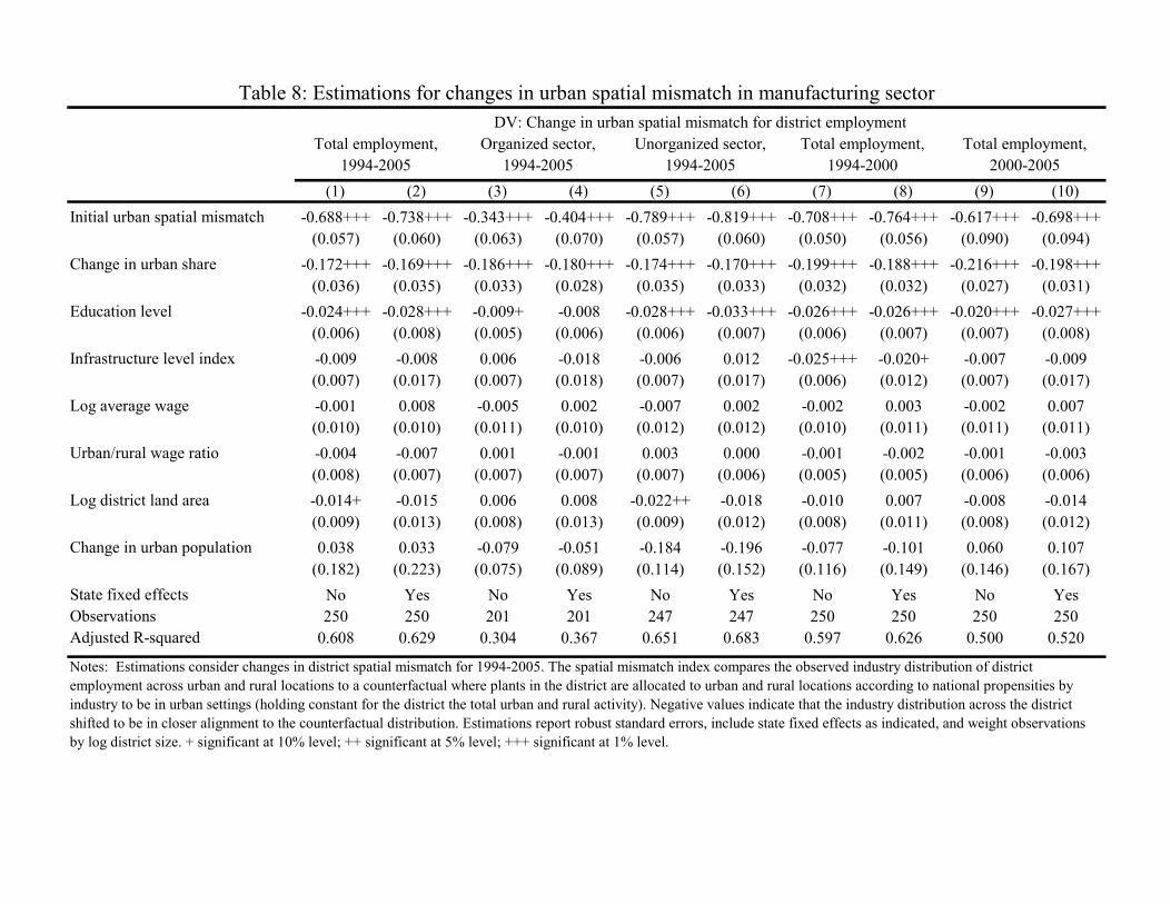
(1) (2) (3) (4) (5) (6) (7) (8) (9) (10)Initial urban spatial mismatch -0.688+++ -0.738+++ -0.343+++ -0.404+++ -0.789+++ -0.819+++ -0.708+++ -0.764+++ -0.617+++ -0.698+++

(0.057) (0.060) (0.063) (0.070) (0.057) (0.060) (0.050) (0.056) (0.090) (0.094)Change in urban share -0.172+++ -0.169+++ -0.186+++ -0.180+++ -0.174+++ -0.170+++ -0.199+++ -0.188+++ -0.216+++ -0.198+++

(0.036) (0.035) (0.033) (0.028) (0.035) (0.033) (0.032) (0.032) (0.027) (0.031)Education level -0.024+++ -0.028+++ -0.009+ -0.008 -0.028+++ -0.033+++ -0.026+++ -0.026+++ -0.020+++ -0.027+++

(0.006) (0.008) (0.005) (0.006) (0.006) (0.007) (0.006) (0.007) (0.007) (0.008)Infrastructure level index -0.009 -0.008 0.006 -0.018 -0.006 0.012 -0.025+++ -0.020+ -0.007 -0.009

(0.007) (0.017) (0.007) (0.018) (0.007) (0.017) (0.006) (0.012) (0.007) (0.017)Log average wage -0.001 0.008 -0.005 0.002 -0.007 0.002 -0.002 0.003 -0.002 0.007

(0.010) (0.010) (0.011) (0.010) (0.012) (0.012) (0.010) (0.011) (0.011) (0.011)Urban/rural wage ratio -0.004 -0.007 0.001 -0.001 0.003 0.000 -0.001 -0.002 -0.001 -0.003

(0.008) (0.007) (0.007) (0.007) (0.007) (0.006) (0.005) (0.005) (0.006) (0.006)Log district land area -0.014+ -0.015 0.006 0.008 -0.022++ -0.018 -0.010 0.007 -0.008 -0.014

(0.009) (0.013) (0.008) (0.013) (0.009) (0.012) (0.008) (0.011) (0.008) (0.012)Change in urban population 0.038 0.033 -0.079 -0.051 -0.184 -0.196 -0.077 -0.101 0.060 0.107

(0.182) (0.223) (0.075) (0.089) (0.114) (0.152) (0.116) (0.149) (0.146) (0.167)State fixed effects No Yes No Yes No Yes No Yes No YesObservations 250 250 201 201 247 247 250 250 250 250Adjusted R-squared 0.608 0.629 0.304 0.367 0.651 0.683 0.597 0.626 0.500 0.520

Table 8: Estimations for changes in urban spatial mismatch in manufacturing sectorDV: Change in urban spatial mismatch for district employment

Notes: Estimations consider changes in district spatial mismatch for 1994-2005. The spatial mismatch index compares the observed industry distribution of district employment across urban and rural locations to a counterfactual where plants in the district are allocated to urban and rural locations according to national propensities by industry to be in urban settings (holding constant for the district the total urban and rural activity). Negative values indicate that the industry distribution across the district shifted to be in closer alignment to the counterfactual distribution. Estimations report robust standard errors, include state fixed effects as indicated, and weight observations by log district size. + significant at 10% level; ++ significant at 5% level; +++ significant at 1% level.

Total employment, 2000-2005

Organized sector,1994-2005

Total employment, Unorganized sector, Total employment, 1994-2005 1994-2005 1994-2000

Plants Employ. Output Plants Employ. Output Plants Employ. Output(1) (2) (3) (4) (5) (6) (7) (8) (9)

Urban share start 0.247 0.376 0.615 0.688 0.667 0.620 0.239 0.302 0.565 Urban share ending 0.294 0.396 0.553 0.626 0.603 0.546 0.285 0.347 0.574 Urban share change 0.047 0.020 -0.062 -0.063 -0.064 -0.073 0.046 0.046 0.009

Within-district component 0.038 0.015 -0.055 -0.089 -0.111 -0.093 0.039 0.036 0.001 Between-district component 0.028 0.013 -0.032 -0.039 -0.045 -0.035 0.022 0.015 -0.033 Covariance term -0.019 -0.008 0.025 0.066 0.092 0.055 -0.016 -0.006 0.041 Total 0.047 0.020 -0.062 -0.063 -0.064 -0.073 0.046 0.046 0.009

Within-district component 0.029 0.011 -0.043 -0.056 -0.065 -0.065 0.031 0.033 0.022 Between-district component 0.018 0.009 -0.020 -0.006 0.001 -0.008 0.015 0.012 -0.013 Total 0.047 0.020 -0.062 -0.063 -0.064 -0.073 0.046 0.046 0.009

Notes: See Table 4.

Appendix Table 1a: Decompositions of urban share changes, 1994-2000

A. Sector change in urbanization level using balanced panel

B. Decomposition: Bailey et al. (1992)

C. Decomposition: Griliches and Rejev (1995)

Total Activity Unorganized SectorOrganized Sector

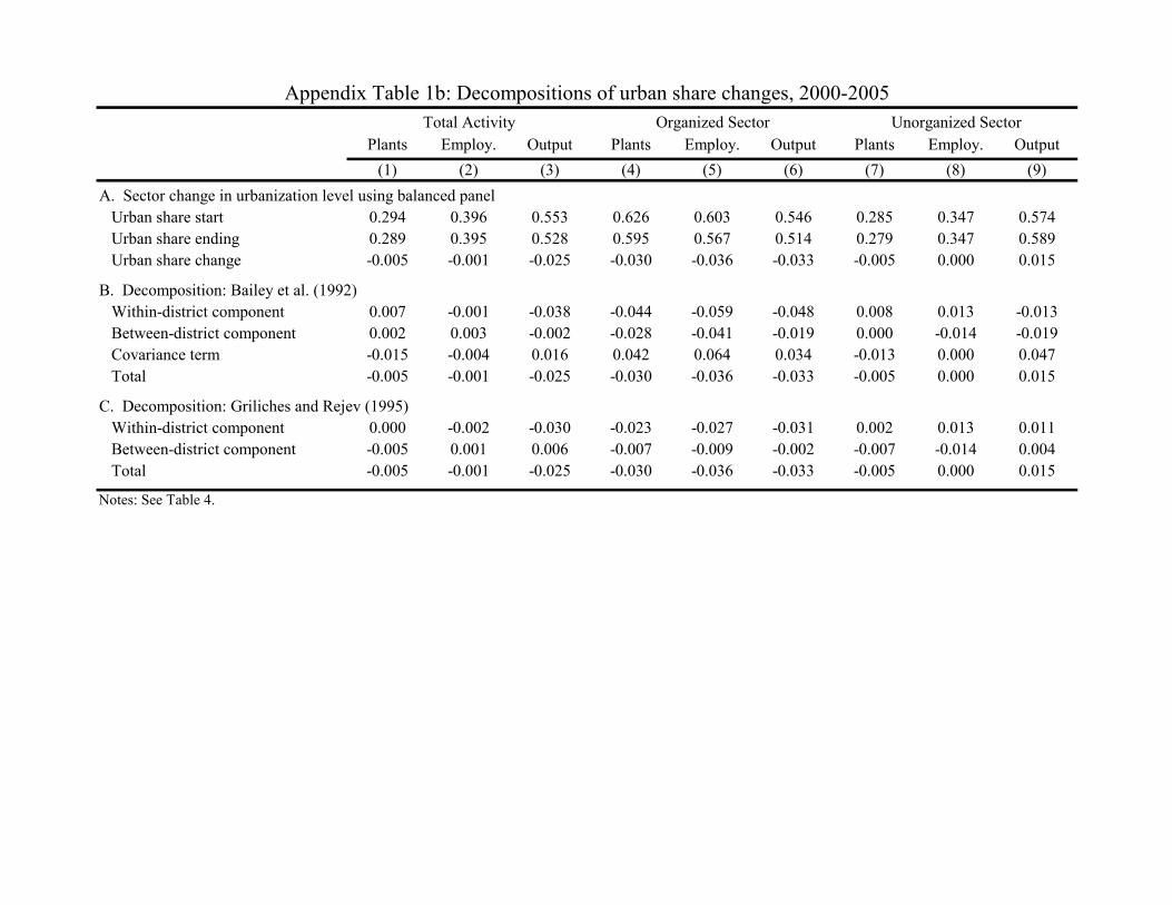
Plants Employ. Output Plants Employ. Output Plants Employ. Output(1) (2) (3) (4) (5) (6) (7) (8) (9)

Urban share start 0.294 0.396 0.553 0.626 0.603 0.546 0.285 0.347 0.574 Urban share ending 0.289 0.395 0.528 0.595 0.567 0.514 0.279 0.347 0.589 Urban share change -0.005 -0.001 -0.025 -0.030 -0.036 -0.033 -0.005 0.000 0.015

Within-district component 0.007 -0.001 -0.038 -0.044 -0.059 -0.048 0.008 0.013 -0.013 Between-district component 0.002 0.003 -0.002 -0.028 -0.041 -0.019 0.000 -0.014 -0.019 Covariance term -0.015 -0.004 0.016 0.042 0.064 0.034 -0.013 0.000 0.047 Total -0.005 -0.001 -0.025 -0.030 -0.036 -0.033 -0.005 0.000 0.015

Within-district component 0.000 -0.002 -0.030 -0.023 -0.027 -0.031 0.002 0.013 0.011 Between-district component -0.005 0.001 0.006 -0.007 -0.009 -0.002 -0.007 -0.014 0.004 Total -0.005 -0.001 -0.025 -0.030 -0.036 -0.033 -0.005 0.000 0.015

C. Decomposition: Griliches and Rejev (1995)

Notes: See Table 4.

Appendix Table 1b: Decompositions of urban share changes, 2000-2005Total Activity Organized Sector Unorganized Sector

A. Sector change in urbanization level using balanced panel

B. Decomposition: Bailey et al. (1992)