Is offshoring driven by air emissions?Testing the pollution haven effect for imports of intermediates

October 2013

Bernhard Michel, bm@plan.be

WORKING PAPER 12-13

Federal Planning Bureau Economic analyses and forecas ts

Avenue des Arts 47-49 – Kunstlaan 47-49 1000 Brussels E-mail: contact@plan.be http://www.plan.be

Federal Planning Bureau

The Federal Planning Bureau (FPB) is a public agency.

The FPB performs research on economic, social-economic and environmental policy issues. For that purpose, the FPB gathers and analyses data, examines plausible future scenarios, identifies alterna-tives, assesses the impact of policy measures and formulates proposals.

The government, the parliament, the social partners and national and international institutions appeal to the FPB’s scientific expertise. The FPB provides a large diffusion of its activities. The community is informed on the results of its research activities, which contributes to the democratic debate.

The Federal Planning Bureau is EMAS-certified and was awarded the Ecodynamic Enterprise label (three stars) for its environmental policy

url: http://www.plan.be e-mail: contact@plan.be

Publications

Recurrent publications: Outlooks Short Term Update

Planning Papers (last publication): The aim of the Planning Papers is to diffuse the FPB’s analysis and research activities. 113 Visions à long terme de développement durable. Concepts, applications et élaboration Langetermijnvisies inzake duurzame ontwikkeling. Begrippen, toepassingen en uitwerking Task Force Sustainable Development - March 2013

Working Papers (last publication): 11-13 De energie-intensiteit van de componenten van de finale vraag 1995-2005 / Een input-output

analyse in constante prijzen Luc Avonds - September 2013

With acknowledgement of the source, reproduction of all or part of the publication is authorized, except for commercial purposes. Responsible publisher: Henri Bogaert Legal Deposit: D/2013/7433/27

WORKING PAPER 12-13

Federal Planning Bureau Avenue des Arts 47-49, 1000 Bruxelles phone: +32-2-5077311 fax: +32-2-5077373 e-mail: contact@plan.be http://www.plan.be

Is offshoring driven by air emissions? Testing the pollution haven effect for imports of intermediates

October 2013

Bernhard Michel, bm@plan.be

Abstract - The pollution haven effect reflects the idea that stricter environmental policies foster the relocation of polluting activities and imports of pollution-intensive products. This paper develops a new approach for testing this effect for imported intermediate materials. It adds to the existing litera-ture on pollution havens through this specific focus on imports of intermediates, which is of particular interest in view of the rise of offshoring within global value chains. The estimation strategy consists in including emission intensities as exogenous demand shifters in a system of cost share equations for variable input factors among which figure imported intermediates. Emissions of three types of air pollutants are analysed: greenhouse gases, acidifying gases and tropospheric precursor gases. The re-sults provide evidence of a pollution haven effect for emissions of acidifying gases, in particular in footloose industries. No such evidence is found for the other types of pollutants. These results reflect the stricter enforcement of regulations for air quality, which act upon acidifying gases.

Jel Classification – F18, F14, Q53, Q56

Keywords - pollution haven effect, trade in intermediates, offshoring, air emissions, translog cost function

WORKING PAPER 12-13

Table of contents

Executive summary ................................................................................................ 1

Synthèse .............................................................................................................. 2

Synthese .............................................................................................................. 4

1. Introduction.................................................................................................... 5

2. Relevant empirical literature .............................................................................. 7

3. Estimation framework ....................................................................................... 9

4. Data sources and descriptive statistics ................................................................. 13

5. Results ......................................................................................................... 17

6. Conclusions ................................................................................................... 21

7. References .................................................................................................... 22

8. Appendix ...................................................................................................... 25

List of tables

Table 1 Summary statistics for cost shares (means across industries), ······································ 14

Table 2 Own-price and cross-price elasticities for variable input factors, cross-industry average

for 2007 ······································································································ 18

Table 3 Elasticities and semi-elasticities for variable input factors with respect to output, capital,

the R&D intensity and emission intensities, cross-industry average for 2007 ····················· 18

Table 4 Robustness checks: semi-elasticities for the demand for import intermediate materials

with respect to emission intensities, cross-industry average for 2007 ····························· 19

List of figures

Graph 1 Cost share of imported intermediate materials (θi) by industry ···································· 15

Graph 2 Emission intensities for three composite air emission indicators (ghgy, acidy, tofpy)

by industry ··································································································· 16

WORKING PAPER 12-13

1

Executive summary

Over the last couple of decades, trade liberalisation has progressed and environmental regulations have become more stringent, in particular regarding emissions of air pollution. This has raised the fear in developed countries that, in order to avoid the growing costs of compliance, emission intensive ac-tivities are increasingly carried out abroad, especially in countries with less stringent regulations. The idea that tighter regulations foster the relocation of polluting activities and imports of pollu-tion-intensive products is generally referred to as the pollution haven effect. If there really is a pollu-tion haven effect, then this has potentially far-reaching consequences for competitiveness as well as for trade policy and environmental policy in developed countries.

The empirical evidence of a pollution haven effect remains relatively scarce despite some supportive findings. However, the literature is mostly based on data for the 80s and 90s and has not yet taken into account the changing nature of globalisation during the last two decades. Trade in intermediates has strongly gained in importance, in particular through the emergence of global value chains, in which production is fragmented and organised at a multi-country level. This leads to offshoring, i.e. the sourcing of intermediates from abroad. While this is facilitated by trade liberalisation and falling transport costs, it is wage cost and productivity differentials that are generally believed to be the main determinants of sourcing decisions. Environmental regulations may also play a role due to the associ-ated compliance costs, i.e. they may foster the sourcing of intermediates from abroad, thereby giving rise to a pollution haven effect for imports of intermediates.

This paper develops an approach for testing the pollution haven effect for imported intermediate ma-terials. The estimation strategy consists in including emission intensities as exogenous demand shifters in a system of cost share equations for variable input factors among which figure imported intermedi-ates. Emissions of three types of air pollutants are analysed: greenhouse gases, acidifying gases and tropospheric precursor gases. The system of cost share equations is estimated with industry-level data for the Belgian manufacturing sector. They come from a time series of constant price supply-and-use tables that have been made consistent with the 2010 vintage of the national accounts. The period cov-ered is 1995-2007. Two major features of these tables are the distinction between domestic and im-ported intermediates and their deflation with separate product-level price indices. The data on emis-sions are drawn from the Belgian air emission accounts.

The results provide evidence of a pollution haven effect for emissions of acidifying gases (SO2, NOX and NH3), in particular in footloose industries (defined in terms of the capital stock per unit of output). This is likely to be linked to the stricter enforcement of regulations for air quality, which act upon acidifying gases. There is no evidence in the results of such a pollution haven effect for emissions of tropospheric precursor gases and in particular of greenhouse gases. Regarding the latter, despite stringent regulations, enforcement appears to be less strict and hence does not seem to influence off-shoring decisions.

WORKING PAPER 12-13

2

Synthèse

Au cours des deux dernières décennies, la tendance à la libéralisation du commerce international s’est poursuivie et dans le même temps les réglementations environnementales ont été rendues plus strictes, en particulier celles concernant les émissions de gaz atmosphériques. Ceci a fait craindre, dans les pays industrialisés, qu’en raison des coûts engendrés par ces réglementations, des activités intensives en émissions soient de plus en plus réalisées à l’étranger, particulièrement dans des pays avec des régle-mentations moins sévères. Dans la littérature, le terme ‘pollution haven effect’ est utilisé pour exprimer cette idée, c’est-à-dire que des réglementations environnementales plus strictes entraînent la délocali-sation d’activités polluantes et l’importation de produits intensifs en pollution. S’il s’avère qu’un tel effet existe, cela pourrait avoir des conséquences pour la compétitivité et la politique commerciale et environnementale des pays développés.

La littérature empirique ne trouve que très peu de résultats qui attestent de l’existence de cet effet. Cependant, la majeure partie des études sont basées sur des données pour les années 80 et 90 et ne prennent donc pas en compte les changements profonds dans la globalisation intervenus au cours des deux dernières décennies. Le commerce de biens intermédiaires a nettement gagné en importance, en particulier à travers l’émergence de chaînes de valeur mondiales, au sein desquelles les processus de production sont fragmentés et organisés par-delà les frontières nationales. L’approvisionnement en biens intermédiaires à l’étranger – appelé ‘offshoring’– en fait partie intégrante. Alors que cette évolu-tion est facilitée par la libéralisation du commerce et la baisse des coûts de transport, les coûts salariaux et les différentiels de productivité sont généralement considérés comme les principaux déterminants des décisions de ‘offshoring’. Les réglementations environnementales pourraient également jouer un rôle en raison des coûts de mise en conformité qui y sont associés. Elles pourraient dès lors favoriser l’approvisionnement à l’étranger, donnant lieu à un ‘pollution haven effect’ pour les importations de biens intermédiaires.

Cette étude propose une approche pour tester le ‘pollution haven effect’ pour les biens intermédiaires importés. Elle consiste à inclure des intensités d’émission dans un système d’équations de parts dans les coûts de plusieurs facteurs, parmi lesquels les biens intermédiaires importés. L’analyse porte sur trois types d’émissions atmosphériques : les gaz à effet de serre, les substances acidifiantes et les pré-curseurs d’ozone troposphérique. Des données par branche d’activité pour le secteur manufacturier belge sont utilisées dans les estimations. Elles proviennent d’une série temporelle de tableaux em-plois-ressources à prix constants, compatibles avec les comptes nationaux de 2010 et couvrant la pé-riode 1995-2007. Deux caractéristiques importantes de ces tableaux sont la distinction entre biens in-termédiaires issus de la production domestique et biens intermédiaires importés, et leur déflation avec des indices de prix distincts par catégorie de produits. Les données sur les émissions proviennent des comptes des émissions atmosphériques pour la Belgique.

Les résultats donnent des indications de l’existence d’un ‘pollution haven effect’ pour les émissions de substances acidifiantes (SO2, NOX and NH3), en particulier pour les branches avec un ancrage géogra-phique faible (défini en termes de stock de capital par unité produite). Cela reflète la mise en applica-tion plus stricte des réglementations en matière de qualité de l’air qui concerne directement les émis-

WORKING PAPER 12-13

3

sions de substances acidifiantes. Par contre, il n’y a d’indications de l’existence d’un tel effet pour les émissions de précurseurs d’ozone troposphérique et surtout pour les gaz à effet de serre. Pour cette dernière catégorie, même si les réglementations paraissent sévères, leur mise en application semble moins stricte, ce qui peut expliquer l’absence d’un impact sur les décisions de ‘offshoring’.

WORKING PAPER 12-13

4

Synthese

De voorbije twee decennia is de handelsliberalisering sterk toegenomen en de milieuregelgeving strenger geworden, vooral wat betreft luchtvervuilende emissies. In industrielanden wekte dit de vrees dat, om de steeds hogere kosten verbonden aan het naleven van die regelgeving te vermijden, emis-sie-intensieve activiteiten steeds meer in het buitenland zouden worden uitgevoerd, vooral in landen met een minder strikte milieuregelgeving. De idee dat een strengere regelgeving de delokalisatie van vervuilende activiteiten en de invoer van vervuilingsintensieve goederen in de hand zou werken, wordt doorgaans het 'pollution-haven' effect genoemd. Indien er zich werkelijk een 'pollution-haven' effect voordoet, heeft dat mogelijks verstrekkende gevolgen voor het concurrentievermogen en voor het handels- en milieubeleid in de industrielanden.

Empirische evidentie voor het bestaan van een 'pollution-haven' effect blijft relatief schaars. De be-staande literatuur is echter meestal gebaseerd op gegevens voor de jaren 80 en 90 en houdt dus geen rekening met de veranderende aard van de globalisering tijdens de laatste twee decennia. De handel in intermediaire goederen is sterk toegenomen, vooral via globale waardeketens waarin de productie over verschillende landen gefragmenteerd en georganiseerd wordt. Dat leidt tot offshoring, namelijk het betrekken van intermediaire goederen uit het buitenland. Handelsliberalisering en lagere trans-portkosten werken dit mee in de hand, maar algemeen wordt aangenomen dat de verschillen in loonkosten en productiviteit de belangrijkste determinanten ervan zijn. Milieuregelgevingen kunnen ook een rol spelen gelet op de eraan gekoppelde kosten voor het naleven ervan; ze kunnen namelijk het betrekken van intermediaire goederen uit het buitenland aanmoedigen en aldus een 'pollution-haven' effect creëren voor de invoer van intermediaire goederen.

In deze paper wordt een methode ontwikkeld om het ‘pollution-haven’ effect te testen voor ingevoerde intermediaire materialen. De strategie bestaat erin emissie-intensiteiten op te nemen als exogene vraag-‘shifters’ in een systeem van kostenaandeelvergelijkingen voor variabele inputfactoren, waartoe ingevoerde intermediaire goederen behoren. De emissies van drie types van luchtvervuilende stoffen worden geanalyseerd: broeikasgassen, verzurende gassen en troposferische ozonprecursoren. Het sys-teem van kostenaandeelvergelijkingen wordt geschat op basis van bedrijfstakgegevens voor de Belgische verwerkende nijverheid. Die gegevens zijn afkomstig van een tijdreeks van aanbod- en gebruikstabellen tegen constante prijzen die coherent zijn gemaakt met jaargang 2010 van de nationale rekeningen. De bestreken periode is 1995-2007. Twee belangrijke eigenschappen van die tabellen zijn het onderscheid tussen binnenlandse en ingevoerde intermediaire goederen en hun deflatie met afzonderlijke prijsindices op productniveau. De emissiegegevens zijn afkomstig van de Belgische luchtemissierekeningen.

De resultaten tonen het bestaan aan van een 'pollution-haven' effect voor emissies van verzurende gassen (SO2, NOX en NH3), vooral in ‘footloose’ industrieën (die laatste worden hier gedefinieerd op basis van kapitaalvoorraad per eenheid productie). Dat is waarschijnlijk het gevolg van de strengere toepassing van de regels voor de luchtkwaliteit, die een impact hebben op verzurende gassen. In de resultaten is geen evidentie terug te vinden voor een dergelijk ‘pollution-haven’ effect voor emissies van trosposferische ozonprecursoren en in het bijzonder van broeikasgassen. Wat die laatste betreft, lijkt de toepassing, on-danks een strenge regelgeving, minder strikt en heeft ze dus geen invloed op beslissingen tot offshoring.

WORKING PAPER 12-13

5

1. Introduction

Over the last couple of decades, trade liberalisation has progressed and environmental regulations have become more stringent, in particular those regarding emissions of air pollution. These two par-allel trends have raised the fear in developed countries that, in order to avoid the growing costs of compliance, emission intensive activities are increasingly carried out abroad, especially in countries with less stringent environmental regulations. The idea that tighter environmental regulations foster the relocation of polluting activities as well as imports of pollution-intensive products is generally re-ferred to as the pollution haven effect (Taylor, 2005). If there really is a pollution haven effect for trade and FDI flows, then this has potentially far-reaching consequences for competitiveness in developed countries as well as for trade policy and environmental policy.

A look at trends in the pollution content of trade should provide a first indication of pollution haven seeking behaviour. But results in the literature rather show the opposite. Analyses of revealed com-parative advantage have failed to produce evidence that developed countries specialise in clean in-dustries (Grether and de Melo, 2004; Cole et al., 2005). Other determinants of specialisation such as capital intensity seem to play a more prominent role (Antweiler et al., 2001). By the same token, articles that examine changes in emissions embodied in trade do not find a systematic shift towards imports of emission-intensive products for developed countries (Ahmad and Wyckoff, 2003; Nakano et al., 2009). According to Levinson (2009), the pollution content of US imports even tends to fall over time, and, according to Dietzenbacher and Mukhopadhyay (2007), the same holds for the emission content of India’s exports.

The evidence of a pollution haven effect is mixed when it comes to econometric estimations of the impact of the stringency of environmental regulations on net exports controlling for other determi-nants. In these estimations, the stringency of environmental regulations is either measured by indicator variables based on survey data or it is proxied by pollution abatement costs or emission intensities. Early country and industry level estimations generally failed to reveal a pollution haven effect (Tobey, 1990; Grossman and Krueger, 1993), while more recent estimations using industry-level panel data for the US provide some support for the pollution haven effect (Ederington et al., 2003; Levinson and Taylor, 2008). Another strand of the literature has tested for a pollution haven effect by including a measure of the stringency of environmental regulations among the determinants of FDI flows. Again, the evidence is mixed. While some US state-level and industry-level analyses do actually find evidence of a pollution haven effect (List and Co, 2000; Keller and Levinson, 2002; Kellenberg, 2009), this is not confirmed by firm-level analyses (Smarzynska and Wei, 2001; Manderson and Kneller, 2012). Overall, despite some supportive findings the evidence of a pollution haven effect remains relatively scarce.

This literature is mostly based on data for the 80s and 90s and it has so far failed to take into account the changing nature of globalisation and trade during the last two decades. Trade has not only been liber-alised and growing fast, but its composition has also been changing. The foremost feature of this change in composition is that trade in intermediates has strongly gained in importance, in particular through the emergence of global value chains (GVCs), in which production is fragmented and organ-ised at a multi-country level (De Backer and Yamano, 2012; Johnson and Noguera, 2012). The reorgan-

WORKING PAPER 12-13

6

isation of production within GVCs shifts production stages to where they can be performed in the most cost efficient way. This leads to offshoring, i.e. the sourcing of intermediates from abroad. While this is facilitated by trade liberalisation and falling transport costs, it is wage cost and productivity differen-tials that are generally believed to be the main determinants of sourcing decisions. Other potential de-terminants are, for example, natural resource endowments or host country institutions and political stability. Environmental regulations may also play a role due to the associated compliance costs. They may induce fragmentation and the transfer abroad of pollution-intensive production stages. Hence, they may foster the sourcing of intermediates from abroad, thereby giving rise to a pollution haven effect for imports of intermediates.

This paper develops an approach for testing the pollution haven effect for imported intermediate ma-terials. The approach is new with respect to the existing literature on pollution havens through its specific focus on imports of intermediates. The test is embedded in a cost function framework from which a system of cost share equations for variable input factors is derived. Within this framework, the demand for imported intermediate materials is explicitly modelled. This is essential for getting a grasp of the drivers of offshoring decisions and whether pollution havens play a role in this respect. The po-tential determinants of the demand for imported intermediate materials include their own price as well as the price of the other input factors. The set of determinants is completed by other demand shifters among which emission intensities for three types of air pollutants. Their impact provides evidence on the pollution haven effect. Note that even if economy-wide uniform environmental regulations are imposed, their effect is still likely to differ across industries according to their pollution intensity, i.e. dirty industries face higher compliance costs and are therefore induced to source intermediate materi-als from abroad. Furthermore, this cost share framework also allows to model simultaneous decisions on quantities of other input factors such as domestic intermediate materials, labour or energy. This is in contrast with the traditional assumption of exogenous factor intensities in the industry-level net export estimations in the previous literature (Grossman and Krueger, 1993; Ederington et al., 2003).

The system of cost share equations is estimated with industry-level data for the Belgian manufacturing sector. They come from a time series of constant price supply-and-use tables that have been made consistent with the 2010 vintage of the national accounts (Avonds et al., 2012). The period covered is 1995-2007, which is much more recent than what is usual in the literature. For example, analyses based on US abatement cost data generally cover the 80s and early 90s. Two major features of these tables are the distinction between domestic and imported intermediates and their deflation with separate prod-uct-level price indices.

This paper is organised as follows. Section 2 provides a more detailed overview of the pollution haven literature. The empirical model and the estimation strategy are described in section 3, while section 4 contains information on data sources as well as descriptive statistics. Estimation results are presented in section 5 and section 6 concludes.

WORKING PAPER 12-13

7

2. Relevant empirical literature

The effect of the stringency of environmental regulations on trade flows and location decisions is the subject of a vast and still growing literature. In this context, Taylor (2005) distinguishes the pollution haven effect (PHE) from the pollution haven hypothesis (PHH). The former arises when tighter envi-ronmental regulations foster the relocation of dirty activities or increase imports and deter exports, while the latter reflects shifts of pollution-intensive industries from countries with stringent environ-mental regulations to countries with lax regulations in response to a fall in trade barriers.1 As empha-sized in Taylor (2005), empirical tests of the PHH are “hobbled with data constraints”. Most notably, there is a need for multi-country data on determinants of trade or investment flows among which the stringency of environmental regulation. Moreover, trade liberalisation must be properly addressed. Hence, it is not surprising that the bulk of the empirical pollution haven literature has treated the PHE rather than the PHH.

A major avenue for testing for a PHE has been to estimate the impact of the stringency of environ-mental regulations on net exports controlling for other determinants of comparative advantage such as factor intensities (physical and human capital), tariff rates and proxies for regulatory stringency on issues not related to the environment. Multi-country analyses based on such a Hekscher-Ohlin (H-O) framework generally fail to find evidence that differences in the stringency of environmental regula-tions2 between countries affect trade flows for dirty industries defined by the share of pollution abatement cost in total cost (Tobey, 1990; Cole and Elliott, 2003). However, the validity of these results is weakened by the fact that they are obtained from cross-section regressions. The results of gravity estimations for bilateral trade flows in van Beers and van den Bergh (1997) – also in cross-section –, and Harris et al. (2002) and Grether and de Melo (2004) – using panel data – confirm the absence of a PHE for dirty industries and also for all industries.3

The H-O estimation framework has also been applied in analyses trying to identify a PHE with detailed industry-level data for the US. In this strand of the literature, it has become standard to use pollution abatement costs as a proxy for environmental regulation. The pioneering contribution in this respect comes from Grossman and Krueger (1993). It evaluates the impact of US environmental regulations on trade between the US and Mexico with regard to the possibility of a North American Free Trade Agreement (NAFTA).4 US industry-level imports from Mexico as a share of total output in 1988 are regressed on the industry-level ratio of pollution abatement cost to value-added, factor intensities and other controls. The results reveal no significant impact of abatement costs on the import share. Again,

1 The PHH is directly derived from theory: in a two-country general equilibrium model à la Copeland and Taylor (1994),

environmental regulation becomes a determinant of comparative advantage when moving from autarky to free trade. 2 Mostly, indicators of the stringency of enironmental regulations are constructed based on qualitative country-level data on

environmental policies as well as cross-country surveys (van Beers and van den Bergh, 1997; Cole and Elliott, 2003). Some-times, other proxies are used such as GDP differences (Grether and de Melo, 2004). This is, however, likely to be a very noisy proxy when it comes to explaining changes in trade flows.

3 Note that van Beers and van den Bergh (1997) do actually find a negative impact of home country regulations on bilateral exports of all goods, but according to Harris et al. (2002) this is essentially due to missing time and country specific effects that cannot be controlled for in a cross-section model.

4 Hence, Grossman and Krueger (1993) really refer to a PHH setting, i.e. whether trade liberalisation within NAFTA has the potential of shifting dirty activities from the US to Mexico where environmental regulations are weaker. However, in their estimations they actually test the PHE.

WORKING PAPER 12-13

8

one of the main weaknesses of this analysis is the cross-sectional aspect of the estimation. Nonetheless, panel data estimations for the US over 1978-1992 with industry and year fixed effects in Ederington et al. (2003) still fail to produce evidence of a significant negative impact of pollution abatement costs on net exports. It is only when net exports are split by partner country that these authors are able to iden-tify a PHE for trade with non-OECD countries.5 Moreover, net exports of more mobile or footloose industries, i.e. those with lower transport and plant fixed costs, appear to be more responsive to abatement cost increases. In a separate paper, the same authors take the analysis one step further by including an interaction term between effective tariff rates and pollution abatement costs (Ederington et al., 2004). This actually comes closer to investigating the PHH. However, the results prove counter-intuitive: polluting industries are found to be significantly less sensitive to tariff reductions.

A further argument for why many empirical tests of the PHE have failed is the potential endogeneity of the stringency of environmental regulations or its proxy, i.e. pollution abatement costs, in net export regressions. Governments may be using environmental policy as a substitute for trade policy when trying to protect industries from import competition (Ederington and Minier, 2003). Hence, regulatory stringency may be responsive to a rise in imports leading to a downward bias in estimations of envi-ronmental regulations on net exports. Ederington and Minier (2003) address this issue by specifying an equation to model pollution abatement costs as a function of net exports and other instruments. Their results confirm the predicted downward bias, although they do not test for instrument validity. Moreover, even at a given level of regulatory stringency, endogeneity may arise when levels of pollu-tion abatement and imports are determined jointly (Levinson and Taylor, 2008). This also casts some doubt on how suitable pollution abatement costs are as a proxy for the stringency of environmental regulation. In the dirtiest or most regulated industries, plant closures and imports may lower pollution abatement costs.6 Again, this would imply a downward bias when estimating the impact of pollution abatement costs on net exports. However, as emphasized by Cole et al. (2005), finding valid instru-ments for abatement costs has proved difficult as trade affects many industry characteristics. Levinson and Taylor (2008) attempt to tackle this problem by relying on instruments based on polluting emis-sions by industry and state within the US. According to their results for US net exports to Mexico and Canada, instrumenting increases the (negative) impact of pollution abatement costs in absolute value thereby confirming the predicted downward bias. However, their estimations do not include factor intensities. Cole et al. (2005) control for physical and human capital intensities in their estimations for total US net exports. Using the same instruments as Levinson and Taylor (2008)7, their results fail to confirm the downward bias. Moreover, the null of instrument validity is rejected by a standard Sargan test in both Levinson and Taylor (2008) and Cole et al. (2005).

5 However, this is not confirmed by a split according to the stringency of environmental standards in the partner country. 6 This may also be influenced by environmental regulations abroad, which are likely to be correlated with both pollution

abatement and imports but are generally unobserved in the industry-level analyses of the PHE for the US (Levinson and Taylor, 2008).

7 Note that there exists a working paper version of Levinson and Taylor (2008) that is prior to Cole et al. (2005).

WORKING PAPER 12-13

9

3. Estimation framework

A distinction between types of traded goods is absent in this literature.8 However, in view of the in-creasing internationalisation of the organisation of production over the last couple of decades as well as the related change in the nature of trade with a growing importance of intermediates, it seems neces-sary to take a closer look at the influence of environmental regulation on imports of intermediates. This is best done within a cost function framework that allows for modelling demands for input factors as a function of relative prices, fixed factors, the scale of output and other exogenous demand shifters. This framework has been popular for estimating the impact of trade on domestic employment by skill-level (Berman et al; 1994; Morrison and Siegel, 2001). Others have done this for offshoring defined as the share of imported intermediates in total non-energy intermediates (Feenstra and Hanson, 1999; Hijzen et al., 2005), which is included as an exogenous demand shifter into the framework. In the model de-veloped here, demand for imported intermediate materials is addressed separately, i.e. total interme-diate materials are split into domestic and imported intermediates and both are treated as variable input factors as in Falk and Koebel (2002). Hence, it becomes possible to estimate the effect of several determinants on the demand for imported intermediates: the relative price of imported intermediates and other domestic variable input factors as well as technological change and pollution intensities. The latter are essential for testing the PHE.

Define the variable cost function as

= , , (1)

where P is a vector of variable input prices, Y a vector of output and quasi-fixed factor quantities, and Z is a vector of demand shifters. For the model exposed here, a non-homothetic translog is assumed as functional form.9 The translog function was introduced into production theory by Christensen et al. (1971). Berndt (1991) provides a detailed description of the translog cost function, which is largely fol-lowed here. Take five variable input factors, labour (l), energy (e), domestic intermediate materials (d), imported intermediate materials (m) and services and other intermediate inputs (s), and consider cap-ital (k) as quasi-fixed. Then, the translog cost function can be written as:

8 Dean and Lovely (2010) distinguish between types of traded goods. They split China’s manufacturing trade into processing

trade and other trade and show that the pollution intensity of processing trade is lower, but they do not estimate a PHE per se.

9 For an example of the use of a different functional form (a generalised Leontief function) within the same framework, see Morrison and Siegel (2001).

WORKING PAPER 12-13

10

= + ∈ + + + ∈

+12 +∈∈12 + 12 + 12 ∈∈

+ ∈ + ∈ + ∈∈

+ + ∈ + ∈

(2)

where I = {l,e,d,m,s} is the set of variable input factors, pi are input prices, y is output and zq are the ex-ogenous demand shifters from the set Q. This cost function is defined for each industry n and time period t, but these subscripts are omitted at this stage for ease of presentation. Although no assumption is made regarding returns to scale (homogeneity with respect to output), homogeneity of degree one with respect to input prices is imposed for given y, k and zq so as to make sure that a proportional in-crease in all variable input factor prices shifts total variable costs by the same proportion. This implies the following parameter restrictions:

∈ = 1, ∈ = ∈ = ∈ = ∈ = ∈ = 0 (3)

Moreover, it is standard to impose symmetry conditions such that:

= , ∀ , ∈ (4)

According to Shephard’s lemma, the cost minimising demand for any variable input factor i (xi) can be obtained by differentiating C with respect to pi. Given the logarithmic form of the translog function, this yields an expression for the cost share (θi) of i in total variable cost.

= = =

= + +∈ + + (5)

From = ∑ ∈ it follows that ∑ ∈ = 1. Equation (5) describes a system of cost share equations. Given the parameters of interest, it is sufficient to estimate this system rather than the entire cost func-tion. For this purpose, error terms ui are added to the share equations. However, as the shares sum to one, the share equations are not linearly independent and the system error covariance matrix is sin-gular. This problem is solved by dropping one equation. The choice is arbitrary but appropriate esti-mation techniques (Zellner’s iterated seemingly unrelated regression estimator) ensure convergence of

WORKING PAPER 12-13

11

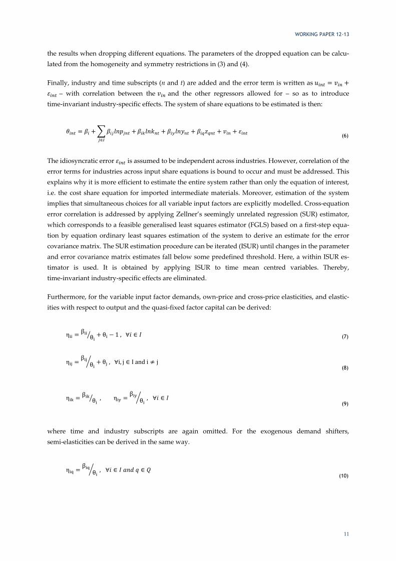
the results when dropping different equations. The parameters of the dropped equation can be calcu-lated from the homogeneity and symmetry restrictions in (3) and (4).

Finally, industry and time subscripts (n and t) are added and the error term is written as = + – with correlation between the and the other regressors allowed for – so as to introduce

time-invariant industry-specific effects. The system of share equations to be estimated is then:

= + +∈ + + + + (6)

The idiosyncratic error is assumed to be independent across industries. However, correlation of the error terms for industries across input share equations is bound to occur and must be addressed. This explains why it is more efficient to estimate the entire system rather than only the equation of interest, i.e. the cost share equation for imported intermediate materials. Moreover, estimation of the system implies that simultaneous choices for all variable input factors are explicitly modelled. Cross-equation error correlation is addressed by applying Zellner’s seemingly unrelated regression (SUR) estimator, which corresponds to a feasible generalised least squares estimator (FGLS) based on a first-step equa-tion by equation ordinary least squares estimation of the system to derive an estimate for the error covariance matrix. The SUR estimation procedure can be iterated (ISUR) until changes in the parameter and error covariance matrix estimates fall below some predefined threshold. Here, a within ISUR es-timator is used. It is obtained by applying ISUR to time mean centred variables. Thereby, time-invariant industry-specific effects are eliminated.

Furthermore, for the variable input factor demands, own-price and cross-price elasticities, and elastic-ities with respect to output and the quasi-fixed factor capital can be derived:

η = β θ + θ − 1 , ∀ ∈ (7)

η = β θ + θ ,∀i, j ∈ Iandi ≠ j (8)

η = β θ , η = β θ ,∀ ∈ (9)

where time and industry subscripts are again omitted. For the exogenous demand shifters, semi-elasticities can be derived in the same way.

η = β θ ,∀ ∈ ∈ (10)

WORKING PAPER 12-13

12

Estimates of these elasticities can be computed using estimated parameters and fitted values for the shares. Elasticity estimates then vary across time periods and industries.

The focus of the analysis is on the elasticities of the demand for imported intermediate materials. In that respect, it is worthwhile repeating that, in the specification developed here, domestic and im-ported intermediate materials are considered as distinct variable input factors. They may be substi-tutes, but this need not be the case, i.e. no a priori restriction is imposed on their elasticity of substitu-tion. The share of imported intermediate materials in total variable cost (θ ) comes very close to what has been defined as (materials) offshoring in the literature, i.e. the share of imported intermediate ma-terials in total non-energy intermediates. Although still referred to as “international outsourcing” at the time, this was pioneered by Feenstra and Hanson (1996). In the framework presented above, θ is ba-sically a current price measure of materials offshoring for total variable cost.

In order to test for a PHE for industry-level imports of intermediates, industry-level pollution intensi-ties are introduced into the translog cost function as exogenous demand shifters ( ). The idea is that more pollution-intensive industries will find it more costly to comply with environmental regulation and that this can to some extent be avoided by sourcing intermediates from abroad. Therefore, the empirical strategy developed here consists in checking whether more pollution-intensive industries have ceteris paribus higher demand for imported intermediate materials. A positive semi-elasticity with respect to pollution intensities may then be considered as evidence in favour of a PHE.

Finally, two further exogenous demand shifters are added to control for technological progress that may alter the variable input factor shares: the industry-level R&D intensity and a linear time trend t. Hence, Q={pollution intensity, R&D intensity, t}. The time trend is also referred to as autonomous tech-nical change, i.e. it is not industry-specific. This may also capture technological progress that contrib-utes to lowering pollution intensities for the entire manufacturing sector.

WORKING PAPER 12-13

13

4. Data sources and descriptive statistics

Data on air emissions from the Belgian air emission accounts (AEA) are used to compute pollution intensities. The AEA are published by the Federal Planning Bureau (FPB) as an environmental satellite account of the national accounts (Janssen and Vandille, 2011). They contain industry-level data on emissions of 15 air pollutants listed in Table A1 in the Appendix. Three composite indicators can be computed from these data, aggregating air emissions according to the type of environmental damage they cause.

– The greenhouse gas index (tonnes of CO2-equivalents):

GHG = 1000*CO2 + 310*N2O + 21*CH4 + PFC + SF6 + HFC

– The acidification indicator (tonnes of H+-equivalents):

ACID = 0.03125 * SO2 + 0.021739 * NOx + 0.058824 * NH3

– The tropospheric ozone forming potential indicator (tonnes of NMVOC equivalents):

TOFP = 1.22 * NOx + NMCOV + 0.11 * CO + 0.014 * CH4

Emission intensities are obtained by normalising by output.10 The level of disaggregation of the emis-sions data is 60 NACE Rev. 1.1 2-digit industries. Focusing on the manufacturing sector restricts the sample to the 23 industries listed in Appendix Table A2. The period covered is limited to the years 1995-2007 in line with the other industry-level data.

Data on quantities and prices of output and intermediate inputs of materials, energy and services11 are taken from supply-and-use tables (SUT) for Belgium. A time series of SUT that are all consistent with the 2010 vintage of the national accounts has been assembled at the FPB for the years 1995-2007 (Avonds et al., 2012). At the most detailed level of disaggregation, the tables cover approximately 120 industries and 320 product categories. For the purpose of the present analysis, they have been aggre-gated to 60 industries (NACE Rev. 1.1 2-digit). As pointed out above, the analysis is then narrowed down to 23 manufacturing industries.

For the model presented above, separate quantity and price data for domestic and imported interme-diate materials are required. These are indeed available from the SUT dataset. On the one hand, the use table is split into a use table for domestic output and a use table for imports for each year. Use tables for imports are constructed based on the methodology described in Van den Cruyce (2004) for the refer-ence years 1995, 2000 and 2005. This method makes use of cross-tabulated import data by firm and product to identify intermediates that have been imported. For non-reference years, use tables for imports are obtained through interpolation of reference year shares of imported intermediates by in-dustry and product and a balancing procedure that ensures that total imports by product category are respected. On the other hand, separate price indices for domestic output and imports for each product

10 Normalisation by value-added for the emission intensities has been tested but did not change the estimation results. 11 This category lumps together service inputs and other intermediate inputs not accounted for by materials and energy, e.g.

agricultural products. As it is largely dominated by the former and for the sake of brevity, this category is referred to in short as services.

WORKING PAPER 12-13

14

category are used to deflate the SUT row-wise. This means that use tables for domestic output and imports are deflated separately with specific price indices. The base year is 2005. Based on the use ta-bles in current prices and the ones in prices of the year 2005, industry-level price indices for interme-diate inputs have been calculated.

Data on labour cost by industry is also directly available from the SUT, while industry-level data on hours worked, i.e. quantities of labour input, are taken from the national accounts. Industry-level wage rates are derived from these two series. Capital stock data are calculated from detailed investment data by product and industry produced by the National Bank of Belgium. The methodology of this capital stock calculation is discussed in Michel (2011). The product-level disaggregation makes it possible to split the capital stock into ICT and non-ICT capital, which are both treated as quasi-fixed factors. Moreover, R&D-intensities at the industry-level are obtained by dividing R&D-stocks by output. R&D stocks are calculated using industry-level data on R&D expenditure from the Belgian Science Policy (Biatour, Dumont and Kegels, 2011). An overview of the data sources is given in Appendix Table A3.

Table 1 reports summary statistics for annual average cost shares. In 2007, spending on imported in-termediate materials represented 35% of total variable cost, which was the biggest share followed by services, labour and domestic intermediate materials. The cost share of energy amounted to only 6%, but it was the one that had grown fastest on average over the period 1995-2007. The shares of services and of imported intermediate materials in total variable cost were also on the rise, while the shares of labour and domestic intermediate materials declined.

Table 1 Summary statistics for cost shares (means across industries), 1995-2007

θl θe θd θm θs sum

Year = 1995 0.274 0.041 0.217 0.292 0.175 1.000

Year = 2007 0.212 0.056 0.173 0.345 0.214 1.000

Absolute change -0.063 0.014 -0.044 0.053 0.039 0.000

Average growth rate -0.021 0.025 -0.019 0.014 0.017

The box plot in Graph 1 gives a flavour of the cross-industry variation in the cost share of imported intermediate materials (θm) for the years 1995, 2002 and 2007. The industries with the largest average θm are motor vehicles (34), basic metals (27) and radio, television and communications equipment (32). The increase in the average θm for all industries documented in Table 1 can also be read from Graph 1. It largely corresponds to the rise in offshoring measured by the share of imported intermediate mate-rials in total non-energy intermediates reported in Hertveldt and Michel (2012).12

12 This is also calculated with SUT data but at a more detailed industry breakdown.

WORKING PAPER 12-13

15

Production in the Belgian manufacturing sector has become cleaner since the mid-90’s. Indeed, emis-sion intensities are downward trending over the sample period for all three composite indicators as illustrated by the falling median values in the box plots in Graph 2. The same downward trend is ob-served for other developed economies (Arto et al., 2012). This can be at least partly attributed to emis-sions reducing technological progress and is captured through the inclusion of a linear time trend in the estimated equations. The box plots also give an idea of the variation in emission intensities across industries. Values outside the interval of the adjacent values are not shown as separate data points in the box plots so as to avoid a scaling of the graphs that conveys the impression that there is only little variation in the emission intensities across industries.13 This graphical ‘winsorising’ of outliers mainly concerns the manufacture of other non-metallic mineral products (26) and basic metals (27), which have by far the highest emission intensity for all three indicators for all years.

13 This does not alter the form of the box plots.

Graph 1 Cost share of imported intermediate materials (θi) by industry

.1.2

.3.4

.5.6

thet

a_i

1995 2002 2007

WORKING PAPER 12-13

16

Graph 2 Emission intensities for three composite air emission indicators (ghgy, acidy, tofpy) by industry

0.0

5.1

.15

.2.2

5gh

g_y

1995 2002 2007excludes outside values

0.1

.2.3

.4.5

acid

_y

1995 2002 2007excludes outside values

01

23

tofp

_y

1995 2002 2007excludes outside values

WORKING PAPER 12-13

17

5. Results

The interpretation of the results is focused on the elasticities of the demand for the five variable input factors. The estimation of these elasticities comprises two steps. First, the system of cost share equations in (6) is estimated by within ISUR dropping one equation. Recall that ISUR ensures convergence of the results whatever the equation that is dropped. Coefficient estimates and standard errors for the entire system are reported in Appendix Table A5. An issue to be addressed in this respect is heteroskedastic-ity. The standard ISUR estimator provides an efficient solution for error correlation across equations, but imposes homoskedasticity for the idiosyncratic error term. As suggested in Cameron and Trivedi (2010, p.166), bootstrapping can be used to obtain heteroskedasticity-robust standard errors in ISUR estimations. Here, bootstrapping implies resampling over industries. Then, the residual variance dif-fers between industries, while independence across industries is maintained. The standard errors re-ported in Appendix Table A5 are heteroskedasticity-robust through bootstrapping.

Second, estimates of the elasticities or semi-elasticities with respect to prices, output, the capital stock and exogenous demand shifters are obtained from the identities (7)-(10). For this purpose the model coefficients (the β’s) are replaced by their sample estimates and the cost shares (the θi’s) are replaced by their fitted values. However, elasticity estimates are different for each industry-year combination. For ease of interpretation, Tables 2 and 3 present estimated elasticities based on average fitted cost shares for the last year in the sample, i.e. 2007. The standard errors for these elasticities are obtained through the delta method, which allows to approximate standard errors for non-linear combinations of coeffi-cient estimates.

Several checks ought to be performed on the estimated translog cost function (Berndt, 1991, p.476). First, for it to be monotonically increasing, the fitted cost shares should all be positive. This is indeed the case for the annual averages. Second, for it to be strictly quasi-concave, the matrix of second-order derivatives with respect to the variable input factor prices – which correspond to the elasticities of substitution between these input factors – should be negative semi-definite at each observation. A matrix is negative semi-definite if its principal minors are of alternating sign starting with a negative first order principal minor. This is highly unlikely to be true for each observation, i.e. industry-year combination. In the shortcut verification using average cross-industry elasticities of substitution for 2007, the fourth order principal minor turns out negative, which means that strict quasi-concavity is likely not given for all observations. Third, parameter restrictions in (3) allow for the derivation of an additivity condition for the own-price and cross-price elasticities in (7) and (8): ∑ ∈ = 0. This pro-vides a useful check for the validity of the calculated elasticities and it is easy to see that this is indeed true for the elasticities reported in Table 2.

The own-price elasticities in Table 2, i.e. the elements on the diagonal, are all negative, which is con-sistent with theory, and they are all smaller than 1 in absolute value. Moreover, the own-price elastici-ties for labour, energy and imported intermediate materials are significant at the 1%-level, and the highest (own-price) elasticity is observed for the latter. The price of services and domestic intermediate materials does not significantly influence demand for these variable input factors. Regarding cross-price elasticities, an increase in the price of imported intermediate materials entails a significant

WORKING PAPER 12-13

18

rise in the demand for all other variable input factors except services. This suggests a rise in domestic production when shifting production stages abroad becomes more expensive. Regarding the demand for imported intermediate materials, it is noteworthy that domestic and imported intermediate mate-rials are substitutes. This corresponds to the expected relationship between domestic factor prices and offshoring. Furthermore, higher wage rates and energy prices also significantly contribute to raising demand for imported intermediate materials. Finally, results in Table 3 show that output growth sig-nificantly fosters demand for imported intermediate materials, while more ICT capital significantly reduces this demand. The elasticities of xm with respect to non-ICT capital and the R&D intensity are not significant.

Table 2 Own-price and cross-price elasticities for variable input factors, cross-industry average for 2007

xl xe xd xm xs

pl -0.548*** -0.564*** 0.122* 0.148** 0.345***

(0.0672) (0.114) (0.0713) (0.0620) (0.0838)

pe -0.163*** -0.762*** 0.113* 0.148*** 0.0526

(0.0343) (0.174) (0.0619) (0.0356) (0.0640)

pd 0.0994* 0.317* -0.254 0.385*** -0.542***

(0.0574) (0.170) (0.208) (0.116) (0.160)

pm 0.234** 0.810*** 0.747*** -0.842*** 0.232

(0.0957) (0.190) (0.229) (0.158) (0.206)

ps 0.378*** 0.199 -0.729*** 0.161 -0.0885

(0.0906) (0.243) (0.212) (0.144) (0.292)

Based on parameter estimates in Appendix Table A5; heteroskedasticity-robust standard errors in parentheses. Significance levels: * p<0.1, ** p<0.05, *** p<0.01.

Table 3 Elasticities and semi-elasticities for variable input factors with respect to output, capital, the R&D intensity and emission intensities, cross-industry average for 2007

xl xe xd xm xs

y -0.390*** -0.0860 0.0756 0.464*** -0.347***

(0.0648) (0.100) (0.197) (0.0767) (0.134)

kict 0.130 0.295* 0.0931 -0.197 0.0194

(0.0921) (0.177) (0.226) (0.126) (0.172)

knonict 0.724*** 0.0642 0.989** -0.0638 -1.323***

(0.192) (0.274) (0.472) (0.205) (0.434)

rdy 0.0142 -0.117 0.192* -0.161*** 0.108

(0.0415) (0.0779) (0.0991) (0.0581) (0.0777)

ghgy 0.847*** 1.443** -0.633* 0.101 -0.831**

(0.154) (0.582) (0.331) (0.220) (0.346)

acidy 0.177* -0.875** -0.346* 0.284* -0.0833

(0.0959) (0.401) (0.209) (0.161) (0.186)

tofpy -0.0399 -0.0265 0.0577 -0.0269 0.0394

(0.0252) (0.0608) (0.0683) (0.0342) (0.0546)

Based on parameter estimates in Appendix Table A5; heteroskedasticity-robust standard errors in parentheses Significance levels: * p<0.1, ** p<0.05, *** p<0.01.

WORKING PAPER 12-13

19

The main elasticities of interest for detecting a PHE are the semi-elasticities of the demand for imported intermediate materials with respect to the emission intensities. They are reported in the bottom three columns of Table 3. Note that in this baseline specification emission intensities are lagged one period so as to avoid contemporaneous feedback from choices regarding variable input factors on emission in-tensities.14 A positive semi-elasticity is evidence of a PHE. Results differ between the three composite indicators. The semi-elasticity is positive significant for ACID, positive but not significant for GHG, and negative non-significant for TOFP. Hence, there is some evidence for a PHE for intermediate ma-terials based on emissions of acidifying gases. According to these estimates, industries with a higher emission intensity for ACID have ceteris paribus greater demand for imported intermediate materials, i.e. on average, they source more materials from abroad. However, this is not the case for elasticity estimates for the other two emission intensities (GHG and TOFP), which are not significant.

Table 4 Robustness checks: semi-elasticities for the demand for import intermediate materials with respect to emis-sion intensities, cross-industry average for 2007

Year fixed effects Dropping industry 26 Footloose industries

ghgy -0.207 0.207 0.763**

(0.183) (0.270) (0.353)

acidy 0.281** 0.438** -0.143

(0.141) (0.209) (0.150)

tofpy -0.0018 -0.0382 -0.0365

(0.0314) (0.0347) (0.0310)

footloose*ghgy -0.612

(0.383)

footloose*acidy 1.062***

(0.303)

footloose*tofpy -0.0457

(0.0975)

Bootstrapped heteroskedasticity-robust standard errors in parentheses Significance levels: * p<0.1, ** p<0.05, *** p<0.01.

Environmental policy provides some guidance as regards the interpretation of the difference in the PHE results for the different types of emissions, i.e. significant positive for ACID and not significant for the other emission indicators, in particular GHG. The air pollutants contained in ACID (SO2, NOX and NH3) are to a large extent associated with air quality. In this field, longstanding policy action has sig-nificantly contributed to reductions in emissions and the improvement of air quality (EEA, 2012, p.65). This policy action has encompassed both stringent regulations and enforcement. Things are different for GHG. Although regulations on GHG emissions are stringent on paper, enforcement has remained lax. As emphasized in Kozluk (2011), practically all Belgian ETS emission permits are grandfathered, i.e. granted for free based on historical emissions. Given this difference in enforcement, it appears as natural that the emission intensity for ACID plays a role in offshoring decisions, whereas for GHG it does not. This confirms the importance of enforcement for the PHE as highlighted in Kellenberg (2009).

14 Estimating the system with contemporaneous emission intensitiesdoes not alter the results significantly. These results are not

reported here but are available from the author.

WORKING PAPER 12-13

20

The PHE results are robust to several sensitivity checks. First, given the relatively high correlation between emission intensities for the three types of air emissions, separate estimations have been run, which include each only one of the three emission intensities. The results do not change in any sub-stantial way.15 Second, the time trend can be replaced by year fixed effects, i.e. the linearity assumption can be released. Results for this robustness check are presented in the first column of Table 4. For the sake of brevity, only the semi-elasticities of xm with respect to the emission intensities are reported.16 The results are similar to those with a time trend, only the elasticity of xm with respect to the GHG emission intensity changes sign but remains non-significant. Third, the descriptive data analysis in the previous section led to the identification of the industry of other non-metallic mineral products (26) as the main outlier in terms of emission intensities for all three composite indicators. Re-estimating the initial specification excluding observations for industry 26 allows to check whether the significant positive semi-elasticity for ACID is driven by this industry. Column 2 of Table 4 shows that the semi-elasticity actually increases when dropping industry 26.

Finally, Table 4 also contains results for a test of the PHE when distinguishing between geographically mobile and other industries (column 3). Previously, Ederington et al. (2005) and Kellenberg (2009) found stronger evidence for a PHE in so-called ‘footloose’ industries, defining such industries as less capital intensive or with lower fixed costs relative to output and thereby more geographically mobile. Following this same approach, the footloose dummy variable created for this test is equal to one for industries with a value of capital stock per unit of output that is below the sample median. Regarding descriptive statistics, ‘footloose’ industries have on average a higher cost share of imported interme-diate materials, however growth in this share is slower than for other industries. Trends in emission intensities are comparable in the two sub-samples. Including interaction effects between the ‘footloose’ dummy variable and emission intensities into the estimation framework yields semi-elasticities for both categories of industries. The results in column 3 of Table 4 reveal that the PHE for ACID is essen-tially driven by footloose industries. There is no evidence of a PHE for GHG or TOFP for either type of industry.

15 The results are not reported here but are available on request. 16 There are only minor changes in the elasticities that are not reported in Table 4. The full estimation results for these robust-

ness checks are available on request.

WORKING PAPER 12-13

21

6. Conclusions

Developments in information and communication technologies and trade liberalisation have contrib-uted, over the last couple of decades, to deeply modifying the nature of international trade by facili-tating the growing cross-border fragmentation of production processes as well as the rise of offshoring. The latter consists in an increase of the sourcing of intermediates from abroad reflected in a growing share of intermediates that are imported. This article adds to the existing literature by looking at the pollution haven effect in this context. In practice, this implies exploring whether environmental policy is a determinant of offshoring. For this purpose, the estimation strategy consists in including emission intensities as exogenous demand shifters in a system of cost share equations for variable input factors. The system is derived from a translog cost function with imported intermediates as one of the variable input factors. This approach basically comes down to estimating a pollution haven effect for imports of intermediates. The focus on imports of intermediates in an input demand framework is new with re-spect to previous trade-based empirical analyses of the pollution haven effect, which have generally looked at total net trade flows in a comparative advantage setting.

According to the estimation results, there is some evidence that footloose industries have fled the stricter enforcement of environmental regulations regarding emissions of acidifying gases (SO2, NOX and NH3), which are linked to air quality. They do so through offshoring, i.e. by fragmenting produc-tion processes and by sourcing intermediates from abroad. There is no evidence in the results of such a pollution haven effect for emissions of tropospheric precursor gases and in particular of greenhouse gases. Regarding the latter, despite stringent regulations, enforcement appears to be less strict and hence does not seem to influence offshoring decisions.

These findings call for further research on the pollution haven effect for imported intermediates. The framework that has been developed here should be extended provided appropriate data become available. On the one hand, it should include other pollutants than air emissions so as to test for the influence of other environmental policies. On the other hand, a split of imports of intermediate mate-rials according to the country of origin could shed some light on whether the pollution haven effect is stronger for intermediate materials sourced from countries with less stringent environmental regula-tions. This depends on the availability of data on prices of imported intermediates by country of origin. Finally, applying this test in a multi-country framework would allow for checking the validity of the results for Belgium that are presented here.

WORKING PAPER 12-13

22

7. References

Ahmad, N. And A. Wyckoff (2003), “Carbon Dioxide Emissions Embodied in International Trade of Goods” OECD Science, Technology and Industry Working Paper 2003/15, Paris

Antweiler, W., Copeland, B. and M. Taylor (2001), “Is Free Trade Good for the Environment?”, Amer-ican Economic Reveiw 91, pp.877-908

Arto, I., A. Genty, J. Rueda-Cantuche, A. Villanueva and V. Andreoni (2012), “Global Resources Use and Pollution / Production, Consumption and Trade (1995-2008)”, JRC Scientific and Policy Reports, European Commission Joint Research Centre

Avonds, L., G. Bryon, C. Hambÿe, B. Hertveldt, B. Michel and B. Van den Cruyce (2012), “Supply and Use Tables and Input-Output Tables for Belgium 1995-2007: Methodology of Compilation”, Federal Planning Bureau, Working Paper 6-12, Brussels

Berman, E., Bound, J. and Griliches, Z. (1994), “Changes in the Demand for Skilled Labor within U.S. Manufacturing: Evidence from the Annual Survey of Manufactures”, The Quarterly Journal of Economics 109 (2), pp. 367-397

Berndt, E. (1991), The Practice of Econometrics: Classics and Contemporary, Reading, MA, Addi-son-Wesley

Biatour, B., Dumont, M. and Kegels, C. (2011), “The determinants of industry-level total factor productivity in Belgium”, Federal Planning Bureau, Working Paper 7-11, Brussels

Cameron, C., and P. Trivedi (2010), “Microeconometrics Using Stata”, Revised Edition, Stata Press, College Station, Texas

Christensen, L., Jorgenson, D. and Lau, L. (1971), “Conjugate Duality and the Transcendental Loga-rithmic Production Function”, Econometrica 39 (4), pp. 255-256

Cole, M., Elliott, R. and Shinamoto, K. (2005), “Why the grass is not always greener: the competing effects of environmental regulations and factor intensities on US specialization”, Ecological Eco-nomics 54, pp.95-109

Cole, M. and R. Elliott (2003), “Do Environmental Regulations Influence Trade Patterns? Testing Old and New Trade Theories”, The World Economy 26 (8), pp.1163-1186

Copeland, B. and M. Taylor (1994), “North-South Trade and the Environment”, Quarterly Journal of Economics 109(3), pp. 755-787

Dean, J. and M. Lovely (2010), “Trade Growth, Production Fragmentation, and China’s Environment”, in R. Feenstra and S. Wei (eds.) China’s Growing Role in World Trade, University of Chicago Press, pp.429-469

De Backer, K. and N. Yamano (2012), “International Comparative Evidence on Global Value Chains”, OECD Science, Technology and Industry Working Paper 2012/03, OECD Publishing, Paris

WORKING PAPER 12-13

23

Dietzenbacher, E. and K. Mukhopadhyay (2007), “An Empirical Examination of the Pollution Haven Hypothesis for India: Towards a Green Leontief Paradox?”, Environmental and Resource Econom-ics 36, pp.427-449

Ederington, J., Levinson, A. and J. Minier (2004), “Trade Liberalization and Pollution Havens”, The B.E. Journal of Economic Analysis & Policy 4(2)

Ederington, J., Levinson, A. and J. Minier (2005), “Footloose and pollution free”, Review of Economics and Statistics 87(1), pp.92-99

Ederington, J. and J. Minier (2003), “Is environmental policy a secondary trade barrier? An empirical analysis”, Canadian Journal of Economics 36 (1), pp.137-154

EEA (2012), “Environmental Indicator Report 2012”, European Environmental Agency, Copenhagen

Falk, M. and B. Koebel (2002), “Outsourcing, Imports and Labour Demand”, Scandinavian Journal of Economics 104 (4), pp.567-586

Feenstra, R. and G. Hanson (1996), “Globalisation, Outsourcing, and Wage Inequality”, American Economic Review, vol. 86, pp.240-245

Feenstra, R. and G. Hanson (1999), “The Impact of Outsourcing and High-Technology Capital on Wages: Estimates for the United States, 1979-1990”, The Quarterly Journal of Economics, vol. 114 (3), pp.907-940

Grether, J. and J. de Melo (2004), “Globalization and Dirty Industries: Do Pollution Havens Matter?”, in R. Baldwin and A. Winters (eds.) Challenges to Globalization: Analyzing the Economics, University of Chicago Press, pp.167-203

Grossman, G. and A. Krueger (1993), “Environmental Impacts of a North American Free Trade Agreement”, in P. Garber (ed.) The U.S.-Mexico Free Trade Agreement, MIT Press, Cambridge, pp.13-56

Harris, M., Konya, L. and L. Matyas (2002), “Modelling the Impact of Environmental Regulations on Bilateral Trade Flows: OECD, 1990–1996”, The World Economy 25 (3), pp.387-405

Hertveldt, B. and B. Michel (2012), “Offshoring and the Skill Structure of Labour Demand in Belgium”, Federal Planning Bureau, Working Paper 7-12, Brussels

Hijzen, A., Görg, H. and R. Hine (2005), “International outsourcing and the skill structure of labour demand in the United Kingdom”, The Economic Journal, vol. 115, pp.860-878

Jaffe, A., Peterson, P., Portney, P. and R. Stavins (1995), “Environmental Regulation and the Competi-tiveness of U.S. Manufacturing: What Does the Evidence Tell Us?”, Journal of Economic Literature 33(1), pp.132-163

Janssen, L. and G. Vandille (2011), “Air Emission Accounts for Belgium (1990-2007)”, Report for Euro-stat, Federal Planning Bureau, January 2011, Brussels

Johnson, R. and G. Noguera (2012), “Fragmentation and Trade in Value-Added over Four Decades”, NBER Working Paper n°18186

WORKING PAPER 12-13

24

Kellenberg, D. (2009), “An empirical investigation of the pollution haven effect with strategic envi-ronment and trade policy”, Journal of International Economics 78 (2), pp.242-255

Keller, W. and A. Levinson (2002), “Pollution abatement costs and foreign direct investment inflows to US States”, Review of Economics and Statistics 84(4), pp.691-703

Kozluk, T. (2011), “Greener Growth in the Belgian Federation”, OECD Economics Department Work-ing Paper 894, Paris

Levinson, A. (2009), “Technology, International Trade, and Pollution from US Manufacturing”, Amer-ican Economic Review 99, pp.2177-2192

Levinson, A. and M. Taylor (2008), “Unmasking the pollution haven effect”, International Economic Review 49(1), pp.223–254

List, J. and C. Co (2000), “The Effects of Environmental Regulations on Foreign Direct Investment”, Journal of Environmental Economics and Management 40, pp.1-20

Manderson, E. and R. Kneller (2012), “Environmental Regulations, Outward FDI and Heterogeneous Firms: Are Countries Used as Pollution Havens?”, Environmental and Resource Economics 51, pp.317-352

Michel, B. (2011), “Stock de capital par branche SUT 1995-2004”, unpublished, internal document, Federal Planning Bureau, Brussels

Morrison, C. And D. Siegel (2001), “The Impacts of Technology, Trade and Outsourcing on Employ-ment and Labor Composition”, Scandinavian Journal of Economics 103 (2), pp.241-264

Nakano, S., Okamura, A., Sakurai, N., Suzuki, M., Tojo, Y. and N. Yamano (2009), “The Measurement of CO2 Embodiments in International Trade: Evidence from the Harmonised Input-Output and Bi-lateral Trade Database”, OECD Science, Technology and Industry Working Papers, 2009/3, Paris

Smarzynska, B. and S. Wei (2001), “Pollution Havens and Foreign Direct Investment: Dirty Secret or Popular Myth?”, NBER Working Paper n°8465

Taylor, M. (2005), “Unbundling the Pollution Haven Hypothesis” The B.E. Journal of Economic Anal-ysis & Policy 4(2)

Tobey, J. (1990), “The Effects of Domestic Environmental Policies on Patterns of World Trade: An Em-pirical Test”, Kyklos 43(2), pp.191-209

van Beers, C. and J. van den Bergh (1997), “An Empirical Multi-Country Analysis of the Impact of En-vironmental Regulations on Foreign Trade Flows”, Kyklos 50(1), pp.29-46

Van den Cruyce, B. (2004), “Use Tables for Imported Goods and Valuation Matrices for Trade Margins - an Integrated Approach for the Compilation of the Belgian 1995 Input-Output Tables”, Economic Systems Research 16, pp.33-61

WORKING PAPER 12-13

25

8. Appendix

Table A1 – Types of air emissions in the Belgian AEA

Name Symbol Unit (evaluation)

Methane CH4 Tonnes

Nitrous oxide N2O Tonnes

Nitrogen oxides NOx Tonnes (NO2 equivalent)

Carbon monoxide CO Tonnes

Carbon dioxide CO2 Thousands of tonnes

Sulphur oxydes SOx Tonnes (SO2 equivalent)

Ammonia NH3 Tonnes

Non-Methane Volatile Organic Compounds NMVOC Tonnes

Particulate matter PM2.5 and PM10 Tonnes (mass equivalent of filter measurements)

Hydrofluorocarbons HFC Tonnes (CO2 equivalent)

Perfluorocarbons PFCs Tonnes (CO2 equivalent)

Sulphur hexafluoride SF6 Tonnes (CO2 equivalent)

Chlorofluorocarbons CFC Tonnes (CO2 equivalent)

Hydrochlorofluorocarbons HCFC Tonnes (CO2 equivalent) Source: Janssen and Vandille (2011)

Table A2 – List of NACE Rev.1.1 2-digit manufacturing industries

Code Description

15 Manufacture of food products and beverages

16 Manufacture of tobacco products

17 Manufacture of textiles

18 Manufacture of wearing apparel; dressing and dyeing of fur

19 Tanning and dressing of leather; manufacture of luggage, handbags, and footwear

20 Manufacture of wood and of products of wood and cork, except furniture

21 Manufacture of pulp, paper and paper products

22 Publishing, printing and reproduction of recorded media

23 Manufacture of coke, refined petroleum products and nuclear fuel

24 Manufacture of chemicals and chemical products

25 Manufacture of rubber and plastic products

26 Manufacture of other non-metallic mineral products

27 Manufacture of basic metals

28 Manufacture of fabricated metal products, except machinery and equipment

29 Manufacture of machinery and equipment n.e.c.

30 Manufacture of office machinery and computers

31 Manufacture of electrical machinery and apparatus n.e.c.

32 Manufacture of radio, television and communication equipment and apparatus

33 Manufacture of medical, precision and optical instruments, watches and clocks

34 Manufacture of motor vehicles, trailers and semi-trailers

35 Manufacture of other transport equipment

36 Manufacture of furniture; manufacturing n.e.c.

37 Recycling

WORKING PAPER 12-13

26

Table A3 – Summary of data sources

Variable Name Data source References

y, e, d, m, s Output, intermediate inputs (+ labour compensation)

Harmonised SUT (FPB1) Avonds et al. (2012)

k Capital stock (ICT and non-ICT) Based on detailed investment

data from NBB2

Michel (2011)

l Labour (hours worked) National accounts data

ghg, acid, tofp Polluting air emissions Air emission accounts Janssen and Vandille (2011)

rd R&D stock Based on R&D expenditure

data from BSP3

Biatour, Dumont and Kegels (2011)

Remarks: 1 Federal Planning Bureau, 2 National Bank of Belgium, 3 Belgian Science Policy (BELSPO)

Table A4 – Summary statistics

Variable Obs Mean Std.Dev. Min Max

θl 299 0.239 0.077 0.018 0.415

θe 299 0.052 0.123 0.000 0.708

θd 299 0.181 0.068 0.019 0.403

θm 299 0.314 0.111 0.067 0.648

θs 299 0.215 0.100 0.056 0.545

lnpl 299 -10.440 0.307 -10.960 -9.094

lnpe 299 -0.104 0.201 -1.038 0.474

lnpd 299 -0.044 0.179 -0.947 0.596

lnpm 299 0.003 0.146 -0.702 0.336

lnps 299 -0.038 0.132 -0.611 0.396

lny 299 8.301 1.338 4.816 10.450

lnkict 299 4.992 1.174 2.188 7.388

lnknonict 299 7.522 1.532 2.679 9.862

rdy 299 0.133 0.216 0.002 0.985

WORKING PAPER 12-13

27

Table A5 – Within ISUR estimation results for the system of cost shares specified in equation (6)

θl θe θd θm θs

lnpl 0.051*** -0.047*** -0.015 -0.020 0.031

(0.014) (0.007) (0.012) (0.020) (0.019)

lnpe -0.047*** 0.011 0.009 0.029** -0.002

(0.007) (0.010) (0.010) (0.012) (0.015)

lnpd -0.015 0.009 0.098*** 0.071* -0.163***

(0.012) (0.010) (0.036) (0.039) (0.036)

lnpm -0.020 0.029** 0.071* -0.057 -0.023

(0.020) (0.012) (0.039) (0.052) (0.047)

lnps 0.031 -0.002 -0.163*** -0.023 0.156**

(0.019) (0.015) (0.036) (0.047) (0.066)

lny -0.082*** -0.005 0.013 0.153*** -0.079***

(0.014) (0.006) (0.034) (0.026) (0.030)

lnkict 0.003 -0.007 0.033** -0.053*** 0.025

(0.009) (0.005) (0.017) (0.020) (0.018)

lnknonict 0.027 0.018 0.016 -0.065 0.004

(0.019) (0.011) (0.039) (0.041) (0.039)

rdy 0.152*** 0.004 0.168** -0.021 -0.303***

(0.041) (0.017) (0.081) (0.068) (0.097)

ghgy 0.177*** 0.087** -0.108* 0.033 -0.190**

(0.032) (0.036) (0.056) (0.073) (0.078)

acidy 0.037* -0.053** -0.059* 0.094* -0.019

(0.020) (0.025) (0.035) (0.053) (0.043)

tofpy -0.008 -0.002 0.010 -0.009 0.009

(0.005) (0.004) (0.012) (0.011) (0.013)

t -0.003*** 0.000 -0.004*** 0.002 0.004***

(0.001) (0.000) (0.001) (0.001) (0.001)

cons 1.188*** -0.496*** -0.341 -0.433 1.083***

(0.207) (0.135) (0.264) (0.467) (0.372)

N 286 286 286 286 286 R2 0.685 0.394 0.207 0.295 0.247

Bootstrap heteroskedasticity-robust standard errors in parentheses (100 replications, seed = 10101) Significance levels: * p<0.1, ** p<0.05, *** p<0.01.