Embed Size (px)
Citation preview
Iso-energy-efficiency: An approach to power-constrained parallel computation
Shuaiwen Song1, Chun-Yi Su
1, Rong Ge
2, Abhinav Vishnu
3, and Kirk W. Cameron
1
1SCAPE Laboratory, Virginia Tech
2Marquette University
3Pacific Northwest National Laboratory
[email protected], [email protected], [email protected], [email protected], [email protected]
Abstract
Future large scale high performance supercomputer systems
require high energy efficiency to achieve exaflops computational power and beyond. Despite the need to understand energy
efficiency in high-performance systems, there are few techniques to
evaluate energy efficiency at scale. In this paper, we propose a
system-level iso-energy-efficiency model to analyze, evaluate and
predict energy-performance of data intensive parallel applications with various execution patterns running on large scale power-
aware clusters. Our analytical model can help users explore the
effects of machine and application dependent characteristics on
system energy efficiency and isolate efficient ways to scale system
parameters (e.g. processor count, CPU power/frequency, workload size and network bandwidth) to balance energy use and
performance. We derive our iso-energy-efficiency model and apply
it to the NAS Parallel Benchmarks on two power-aware clusters.
Our results indicate that the model accurately predicts total system
energy consumption within 5% error on average for parallel applications with various execution and communication patterns.
We demonstrate effective use of the model for various application
contexts and in scalability decision-making
Keywords: Iso-energy-efficiency, Performance Isoefficiency,
Power Consumption, Power-Aware Clusters.
I. INTRODUCTION
As we enter the era of exascale computing, energy
consumption of large scale parallel systems and data centers
has become one of the most significant hindrances for
designing highly scalable data intensive applications and
larger parallel systems. For instance, recommendations in a
recent report from the US Department of Energy suggest the
power consumption of an exaflop machine, capable of a
1000-fold performance increase over current petaflop
systems, must be constrained to a 10-fold increase in power
consumption [1]. This engineering challenge coupled with
the high operational costs and system failure rates
associated with many-megawatt computing resources has
increased the need to consider power and the entangled
effects of performance in emergent exascale systems and
applications.
Research[2-5] in high-performance power-aware
computing has focused on identifying power saving
opportunities in communicat ion phases and applying DVFS
[6] (dynamic voltage and frequency scaling) strategies to
these phases to reduce power consumption without
sacrificing performance. Figure 1 depicts the types of
controllers used in these techniques to build sophisticated
power management software. The focus in previous work
has been developing a controller that uses observational data
and (in later techniques) predictive data to schedule power
states and balance performance.
Figure 1. Past and current approaches to power
management in high-performance systems.
A key limitat ion of past approaches is a lack o f power-
performance policies allowing users to quantitatively bound
the effects of power management on the performance of
their applicat ions and systems. Existing controllers and
predictors use policies fixed by a knowledgeable user to
opportunistically save energy and minimize performance
impact. While the qualitative effects are often good and the
aggressiveness of a controller can be tuned to try to save
more or less energy, the quantitative effects of tuning and
setting opportunistic policies on performance and power are
unknown. In other words, the controller will save energy
and minimize performance loss in many cases but we have
litt le understanding of the quantitative effects of controller
tuning. This makes setting power-performance policies a
manual trial and erro r process for domain experts and a
black art fo r practit ioners. To improve upon past approaches
to high-performance power management, we need to
quantitatively understand the effects of power and
performance at scale.
We use a modeling based approach that captures power-
performance tradeoffs system-wide and at scale. Our basic
idea is to apply the concept of iso-efficiency [7] for
performance, or the ability to maintain constant per-node
performance as a system scales, to power-performance
management. We want to create techniques that allow us to
quantitatively control and maintain power-performance as
systems and applications scale; we thus name our approach
iso-energy-efficiency. In conducting this work, we found the
first essential step toward controlling for iso-energy-
efficiency was to create a detailed, sophisticated, accurate
model of the effects of performance and power on scaled
systems and applications.
The contributions of this work include:
controller system
sensor predictor
policyuser
Measured error
System input
System output
Measured output
Prediction data
Measured output
Focus of previous work

Development of a fine-grained, analytical iso-energy-
efficiency model that incorporates parallel system
components and computational overlap at scale.
Accuracy analysis and verification of the model on two
power-scalable clusters.
Creat ion of a set of open source tools for deriving and
measuring model input parameters.
Results from a detailed power-performance scalability
analysis of EP, FT and CG from the NAS Parallel
Benchmarks [8], including use of the iso-energy-
efficiency model to bound and maintain system energy
efficiency at scale.
To the best of our knowledge, this is the first system-
level, scalable, analyt ical model of both power and
performance on real systems and applications. We begin the
succeeding discussions with some related work followed by
an overview of the model. Next , we show validation and
results using the model to perform scalability analysis of the
NAS Parallel Benchmarks. Lastly, we show fu ll derivation
of the model and its parameters and conclusions.
II. RELATED WORK
A. Isoefficiency
According to Amdahl’s law [9], speedup for parallel
systems is limited by the amount of parallelis m inherent in
the application. This law characterizes the performance
impact of parallelism. Though there are several other
alternative viewpoints on speedup, the most relevant to our
work is that of Grama et al [7] who proposed a formal
performance isoefficiency function describing how ideally
performance efficiency will remain constant relative to the
smallest node configuration.
Figure 2a. FT performance and energy efficiency.
For a fixed problem size, Figures 2a and 2b show the
performance efficiency curves for FT and CG. FT scales
reasonably well while CG drops off at 16 CPUs then
recovers relative to the ideal case. There are a p lethora of
performance analysis tools and techniques available to help
us interpret and understand an application’s scalability.
These analyses may suggest any number of root causes that
can be addressed to improve isoefficiency.
In contrast, just measuring energy use is challenging for
non experts. Figures 2a and 2b show the energy efficiency
for FT and CG. Moreover, even though the energy
efficiency (o r lack thereof) in these applications is obvious
as they scale, there are few tools currently availab le to
explain the observed energy efficiency.
Figure 2b. CG performance and energy efficiency.
Being able to identify the root cause of energy
inefficiency would allow us to improve system and
application efficiency more in line with the ideal isoefficient
case. However, analyzing and potentially pred icting energy
efficiency is exceed ingly difficult since we must identify
and isolate the interacting effects of power and performance.
For example, changing the power settings on a processor
using DVFS affects performance which in turn potentially
affects the length of time an application takes to complete
which is key to its overall energy usage.
B. Parallel performance models
There has been extensive research conducted on
performance speedup and scalability of parallel applicat ions
in high performance computing. As mentioned, Amdahl’s
law [9] introduced the concept that the speedup is limited by
the fraction of the workload that can be computed in parallel.
Grama et al [7, 10] formally defined isoefficiency as
discussed. The fixed-time speedup model [11], memory-
bounded speedup model [12], and other related studies[13,
14] all extend Amdahl’s law in unique ways. However, all
of these approaches focus on performance and ignore both
energy consumption and the performance effects of power
management.
C. Energy efficiency in HPC
Several h igh-profile efforts such as the Top500 List [15],
the Green500 List [16], the SPECPower benchmark [17],
and power-performance evaluation of the HPCC
benchmarks [18, 19] have elevated the interest in energy
efficiency for high-end systems and servers.
0.7
0.75
0.8
0.85
0.9
0.95
1
1 2 4 8 16 32
Performance Efficiency
Energy Efficiency
Number of CPUs
0.7
0.75
0.8
0.85
0.9
0.95
1
1 2 4 8 16 32
Performance Efficiency
EnergyEfficiency
Number of CPUs
Efficien
cy
Efficien
cy

Ge et al proposed the PowerPack [20] framework for
measuring correlated power and performance data on large
scale systems and we use this framework to collect the
results presented. Early work to improve the efficiency of
high-end systems [3, 4, 21, 22] used various DVFS
scheduling strategies to gain significant energy savings
under performance constraints. Freeh et al [2, 23, 24]
similarly studied energy-performance tradeoffs for MPI
applications.
Our proposed iso-energy-efficiency model analyzes and
predicts the combined effects of performance and power on
scalable systems. The policy module highlighted in Figure 1
is a practical application of improved understanding of the
power-performance tradeoffs and contrasts our work with
approaches to energy efficiency in HPC which have
historically focused on improving controllers and predictors.
The iso-energy-efficiency approach will improve our
understanding of power-performance to quantitatively
bound the impact of power management on performance.
D. Energy modelling
The power-aware speedup model proposed by Ge and
Cameron [25] is a generalization of Amdahl’s Law for
energy. While this model accurately captures some of the
effects of energy management on speedup, it provides little
insight to the root cause of poor power-performance
scalability.
In contrast, the iso-energy-efficiency model generally
predicts energy consumption as the system scales up
allowing direct analysis and comparison of the tradeoffs
between various model parameters.
The Energy Resource Efficiency (ERE) metric proposed
by Jiang et al [26] defines a link between performance and
energy variations in a system to clearly h ighlight the various
performance-energy tradeoffs. As with other models that
identify energy efficiency, this model analyzes at a very
high-level and does not identify causal relat ionships with
poor metric results.
The energy model proposed by Ding et al [27] uses
circuit -level simulation to analyze power-performance
tradeoffs. While th is model shows promise for circuit-level
design, it is too unwieldy for use in analyzing existing large-
scale power-scalable clusters. The model also makes a
number of simplify ing assumptions such as homogenous
workloads and no computational overlap making it less
practical for modeling real systems.
III. ISO-ENERGY-EFFICIENCY MODEL
Here we briefly describe the iso-energy-efficiency
model fo r evaluating the power-performance tradeoffs of
parallel applications and systems. The derivation of the
model is described in detail in Section 6. Tables 1 and 2
provide a summary of all model parameters. Let be the total energy consumption of sequential
execution and be the total energy consumption of parallel
execution for a g iven application on p parallel processors.
Table 1 Machine-depended parameters
Table 2 Application-depended parameters
Let represent the additional energy overhead required
for parallel execution:is the energy overhead for parallel execution.
- (1).
We now define iso-energy-efficiency (EE) as:
(2).
Parameters Definition
Total on-chip computation workload Total off-chip memory access workload. Total parallel computation overhead Total number of memory access overhead
in parallelization Total number of messages packaged in
parallelization
Total number of bytes transmitted P Number of homogeneous processors available
for computing the workloads N Workload or total amount of work(in
instructions or computations)
the extent of overlap among computation, memory access and network transmission
Total overhead time due to parallelism
Total execution time of an application running on a single processor
parameters Definition Time related
[28], Average time per on-chip
computation instruction (including on-chip caches and registers)
Average memory access latency Average start up time to send a message Average time of transmitting a 8-bits word
Total I/O access time Power-related
Average CPU power in running state Average CPU power in idle state
Average memory power in running state Average memory power in idle state
Average IO device power in running state Average IO device power in idle state
Average sum of other devices’ power such
as motherboard, System/CPU fans, NIC, etc. Average system power on idle state
f The clock frequency in clock cycles per second

Let EEF=
be the energy efficiency factor (EEF). EEF
is the ratio of parallel energy overhead to the energy of an
application running sequentially. An application with a large
EEF has low energy efficiency, and vice versa. Effect ive
use of the iso-energy-efficiency model (EE) requires
accurate estimation of the EEF. We can more accurately
estimate EEF using the following equation:
EEF=
=
(3).
EE then becomes:
EE=
=
=
(4).
Equations (3) and (4) form the basis for computing iso-
energy-efficiency. The challenge is to capture each of the
parameters used in these equations for a given application
and system combination.
Tables 1 and 2 show the model parameters used to
calculate EEF and EE can be classified as either machine-
dependent or application-dependent. The machine-
dependent variable vector can be described as a function of
frequency (i.e. computational speed) and workload
bandwidth (i.e. computational throughput) of the hardware:
The application-dependent variable vector can be
described as a function of the amount of parallelism
available and the workload for the application:
Section 6 provides details describing and motivating the
use of these parameters. The reader may skip to this section
to learn more about the iso-energy-efficiency model
derivation or continue to the next two sections where we
validate the iso-energy-efficiency model and demonstrate its
usefulness for evaluating parallel power-performance
efficiency.
IV. TEST ENVIRONMENT AND MODEL VALIDATION
A. Test Environment
We use two different power-aware clusters to conduct our experiments: SystemG and Dori. The SystemG 22.8
TFlop supercomputer provides a research platform for development of high-performance software tools and
applications at scale. It utilizes 325 Mac Pro computer nodes and each node has two 4-core 2.8 Ghz Intel Xeon Processors.
Each node has an 8 GB RAM and each core has a 6 MB
cache. SystemG is equipped with Mellanox 40Gbytes/sec end to end InfiniBand adapters and switches which
dramatically increases the transmission bandwidth and reduce the latency. Since G stands for ‘green”, SystemG is a
power-scalable system and has over 10,000 power and thermal sensors. DVFS, concurrency throttling and dynamic
thermal monitoring enabled. Intelligent Power Distribution
Units (Dominion PX) are attached to adjacent machines so users can dynamically profile power consumption of
controlled machines or remotely turn on/off nodes, etc. The Dori system is composed of 8 nodes and each node
contains dual core AMD Opteron Processor dusl processors. Each node has 6 GB RAM and each core has 1 MB cache.
Dori is equipped with 1 Gbytes/sec Ethernet and switches. PowerPack 2.0 [18, 20], designed and implemented by
the SCAPE Laboratory at Virginia Tech, is a framework for
power/energy profiling, analysis and prediction of parallel applications and systems. The PowerPack infrastructure is
composed of both hardware and software components: the hardware is responsible for accurate and reliable direct
measurement of both system-wide and component level power consumption and the software automatically collects,
processes and synchronizes power data with system load. We
used the PowerPack toolkit for all of the power and performance measurements obtained herein on both clusters.
The NAS Parallel Benchmarks consist of 5 kernels and 3
pseudo-applications that mimic the computation and data
movement characteristics of large scale CFD applicat ions
which are widely used in HPC community. We validate the
proposed model on both systems for the NAS Parallel
Benchmarks. We conducted scalability studies for 3
benchmarks (FT, CG, EP) on SystemG.
B. Model Validation
To validate the iso-energy-efficiency model, we need to
verify the correctness of the model single and parallel
processor configurations. We vigorously measure and derive
the parameters from Tables 1 and 2; namely the machine
and application dependent parameters.
For the machine-dependent parameters, we built a tool
using the Perfmon API from UT-Knoxville to automatically
measure the average (time per on-chip computation
instruction) derived as
. We use the lat_mem_rd
function from the LMbench microbenchmark [29] to
estimate memory costs is obtained by
using the MPPTest tool [30] fo r both the InfiniBand [31]
and Ethernet interconnects in the two clusters . In addition,
can be obtained by using
PowerPack [20]. We d id not include d isk I/O in our
estimations for our energy efficiency model because the
applications we tested are not disk intensive. We leave this
to future work. For completeness, though it is not used in
the current study, we were able to estimate can be
estimated by using the Linux pseudo file /proc/stat.
For the applicat ion-dependent parameters, we build a
workload and overhead model for each parameter by

analyzing the algorithm and measuring the actual workload
for each application. We use Perfmon to measure each
workload parameter, and we use the TAU
performance tool from the University of Oregon to measure
M and B. Figure 3 illustrates the accuracy of the energy
model for P processors. (Note: Specifically, these results are
for Equation (15) in the derivation Section 6).
Figure 3 compares the energy consumption predicted by
the iso-energy-efficiency model with the actual energy
consumption obtained using the PowerPack framework on
Dori for p=4. We repeated all experiments five t imes to
reduce measuring errors. The results indicate that the
proposed energy model can accurately predict the actual
energy consumption within 5% prediction error. We
conducted similar experiments on SystemG. for p=1, 2, 8,
16, 32, 64, 128. Figure 4 shows the average error rate of EP,
FP, and CG applicat ions on SystemG under different levels
of parallelism using the InfiniBand interconnect. The results
show good accuracy. Upon detailed analysis, the relatively
higher errors (8.31%) found with CG were due to
inaccuracies in our memory model fo r this application.
Improving the accuracy for CG is the subject of future work.
Based on the accuracy results for both SystemG and
Dori clusters, we conclude that our iso-energy-efficiency
model performs well on d ifferent network interconnection
infrastructures and can predict total system energy
consumption with an average of 5% prediction error rate for
parallel applications with various execution and
communicat ion patterns.
V. EXPERIMENTAL RESULTS
A. Energy consumption and efficiency prediction for large
scale systems
Given the accuracy of our modeling techniques as described in the previous section, we use measurements from
smaller configurations to predict and analyze power-
performance tradeoffs on larger systems. (Note: we build our
energy consumption and efficiency models using Equations (13), (15), (18), (21) from Section 6 applied a smaller
representative portion of a large scale system. Initially, we obtain machine-dependent variables from
the smaller system and use these values and our models to predict values for increasing number of nodes:
All variables can be measured as described in the previous section. Frequency-dependent variables can be combined by
normalizing measurements obtained through the use of hardware counters, LMbench, MPPTest and Powerpack. For
example, can be described as
sec on SystemG.
We assume power is proportional to ( ≥1).
Next, we model application-dependent variables from the smaller system:
Except for , all of these variables in depend on a
performance model and can be described as a function of problem size, n, and the level of parallelis m, p. For example,
could be described as in one-dimensional,
unordered and radix-2 binary exchange Fast Fourier Transform. With all parameters accounted for, we can solve
for Equations (3) and (4). (Note: Specifically, we first solve Equations (13), (15), (18), and (21) described in the next
section.) We can then project values for larger values of p to predict the power-performance behavior and tradeoffs of
large scale systems.
B. Scalability studies for NAS PB
In this section, we analyze the power-performance
characteristics of FT, EP and CG using the iso-energy-
efficiency approach. We isolate power-performance
efficiency problems and use the model findings to tune
parameters such as problem size, n, CPU clock frequency, f,
and level of parallelis m, p to improve efficiency.
Figure 3. Model validation on Dori system. All the
applications run on 4 nodes under same CPU clock
frequency. Model accuracy for all the benchmarks are
over 95 %.
0
50000
100000
150000
200000
En
ergy
(Jo
ule
)
NAS benchmark suites
Energy Model Validation on Dori System
Actual Measurement (Joule)Estimation By Energy Model(Joule)
Figure 4. The average error rate of EP, FT and CG
program. class=B in node number p= 1,2,4,8,16,
32,64,128.
0.00%
5.00%
10.00%
EP FT CG
6.64%4.99%
8.31%
Average error rate on SystemG
(P=1,2,4,8,16,32,64,128)
Erro
r rate

In each case, we use the methods described in the
previous sections to obtain model para meters and build our
model from measurements on a smaller system. Once we’ve
identified estimates for
and
vectors, we build EE and EEF as described in
Equations (3) and (4). In the rest of this section, all the
parameterizations are obtained for the SystemG cluster
though the same methodology can be applied other
platforms.
1) FT
FT computes a 3-D part ial d ifferential equation solution
using Fast Fourier Transforms. The applicat ion stresses the
CPU, memory and the communication network during
various phases. Parallel FT iterates through approximately
four phases during the execution: computation phase 1,
reduction phase, computation phase2 and all-to-all
communicat ion. The FT benchmark is communication
intensive with dominating parallel communication overhead
for the all-to-all phase. FT has a large memory footprint
compared to the EP (Embarrassingly Parallel) applicat ion in
the NAS suite.
We use the Pairwise exchange/Hockney model [32, 33]
to estimate the MPI_Alltoall operations required to solve for
EE and EEF. (Note: This replaces the general approach to
communicat ion estimat ion described by Equation (17) in the
next section.) By analyzing the FT’s Alltoall
communicat ion algorithm on the architecture of the
SystemG cluster, we found the Pairwise exchange/Hockney
model appropriate and accurate in our validation testing.
The time duration fo r this implementation is described as
follows:
.
In the equation above, is the message size, is
message start up time, and is the transmission
time. For details, please refer to the original paper [32]. We
use our own measurements, MPPTest and the PowerPack
framework to obtain the machine dependent parameters:
Figure 5: 3D plot of with p and f as variables.
In the equation above, for simplicity, we set γ=2 based
on our test bed System G. We analyze FT and measure the
actual workload by observing on-chip executing instructions,
L1, L2 cache misses, main memory accesses and total
instructions using Perfmon to obtain:
= (0.86, 1.06 n, 9.49n, 4.46 , -0.73
)
We then solve for :
,
and thus for we obtain:
.
Figure 5 plots EE with a fixed workload size n. We can
see the level of parallelism, p, most affects changes in
energy efficiency versus frequency (or DVFS power states).
In fact, for this code, frequency f has little impact on energy
efficiency. FT is dominated by all-to-all communicat ions
and synchronizations which makes it less likely to be
influenced by changes in CPU frequency. As the number of
processors scales, the effects of CPU clock frequency on on-
chip workload diminishes eventually while the increasing
effects of parallel overhead and memory dominate. Thus,
for fixed workloads on FT, increasing p will d ramatically
decrease the energy efficiency.
En
ergy efficien
cy
(GHz)

Figure 6: 3D plot of , Assume constant frequency f=2.8GHz with p and n as variables.
Figure 6 illustrates when frequency fixes to
2.8GHz since frequency does not affect energy efficiency.
We can see p still dominates the variance of energy
efficiency. It is also obvious that increasing the problem size,
n, does enhance the energy efficiency.
2) EP
In parallel computing, an embarrassingly parallel (EP)
workload has little inter-processor communicat ion between
parallel processes. EP in the NPB benchmarks generates
pairs of Gaussian random deviates using Marsaglia polar
method. It separates tasks with little or no overhead. Results
of EP can also be considered as a reference of peak
performance of a given machine. We use our measurements,
MPPTest and the PowerPack framework to obtain the
machine dependent parameters :
After analyzing the parallel EP codes, we have:
= (0.93, 109.4*n, 1.03 *n, 0, 6.7 *n *(p-1), 0, 0)
Since communication in embarrassingly parallel is trivial, we simply set M and B to zero in .
Thus, from Equation (19), we have :
So becomes:
Figure 7 3D plot of with p and f as variables
Figure 7 illustrates the variation of . This figure
indicates that energy efficiency hardly changes with p and f.
Energy efficiency is close to 1 for different combinations of
p and f because only minimum communication overhead is
imposed. Since th is is nearly ideal iso-energy-efficiency, we
cannot improve the energy efficiency by scaling problem
size n at all because increases as fast as .
Figure 8 3D plot of , Assume frequency f=2.8GHz, with p and n as
variables.
3) CG
The NAS CG benchmark evaluates a parallel system’s
computation and communication performance. It uses the
conjugate gradient method to find out the smallest
eigenvalue of a large, sparse matrix. It solves a sparse linear
algebra problem which is common to scientific applicat ions
on large-scale systems. We first obtain the machine-
depended parameters using the previous methods:
For the application-dependent parameters we obtain:
= (0.85, 2.13 , 0.96 , 1.86
,-4.75 ).
Thus, we solve for :
En
ergy efficien
cy
En
ergy efficien
cy
En
ergy efficien
cy
(GHz)

=
,
and then for :
.
Figure 9 3D plot of , Assume problem size n=75000, with p and f
as variables.
From , we plot the relationships
between level of parallelism, p, problem size, n and
frequency, f. In Figure 8, we first fix the frequency f at 2.8
GHz to examine the relation between p and n. We notice
that the energy efficiency decreases as p increases. However,
increasing the workload size, n, will improve the energy
efficiency.
Fixing the workload size n, we next observe the
relationship between p and f. Figure 9 shows energy
efficiency declines with increase in the level of parallelis m.
In contract to EP, the energy efficiency increases with CPU
frequency. Digging further to examine the energy overhead
and energy consumption of , we observe both increase
when frequency increases. However, the decreases
while frequency increases because increases faster than
. In this strong scaling case, users can scale the frequency
up using DVFS to achieve better energy efficiency. Also,
compared to FT (see Figure 6), the effects of frequency
have more impact on the on-chip workload of CG than FT
as p scales due to a lower communication to computation
ratio.
4) Discussion of
We classify , and into machine-
dependent variables because their behaviors are highly
related to Chip’s and frequency, f. However, they are
not only affected by machine architecture but also affected
by traits of application. The execution pattern of an
application could also affect the power consumption during
execution. For simplicity, we assume they are only affected
by hardware. From Kim, et al [6, 34], we assume power is
proportional to ( ≥1). Different hardware architecture
could result in different value.
5) Discussion of the effect of the level of parallelism, p We can rewrite Equation (16) as follows to see the
relation between and p when the workload is evenly divided among processers (homogeneous workload):
Thus, is (k ). Generally speaking, more parallelization will incur lower energy efficiency. In this case,
the application’s tasks among all nodes require extra computation, memory accesses and communication efforts to
coordinate with each other to complete the job. We observe this phenomenon in FT and CG. In contrast, EP incurs
almost no overhead and energy efficiency doesn’t decrease
significantly with the increase of the levels of parallelizat ion.
6) Discussion of problem size n. Problem size is a dominant factor affecting energy
efficiency. The EE for applications FT and CG improve if the problem size scales. However, increasing problem size
does not necessarily improve energy efficiency as in the case of EE for EP.
7) Discussion of frequency, f Decreasing frequency can either increase or decrease energy
efficiency. For EP and FT, we observed no energy efficiency improvements for parallel execution when we adjust to low
frequency. However, in the case of CG, we found that higher frequencies can improve energy efficiency because the
memory overhead value decreases.
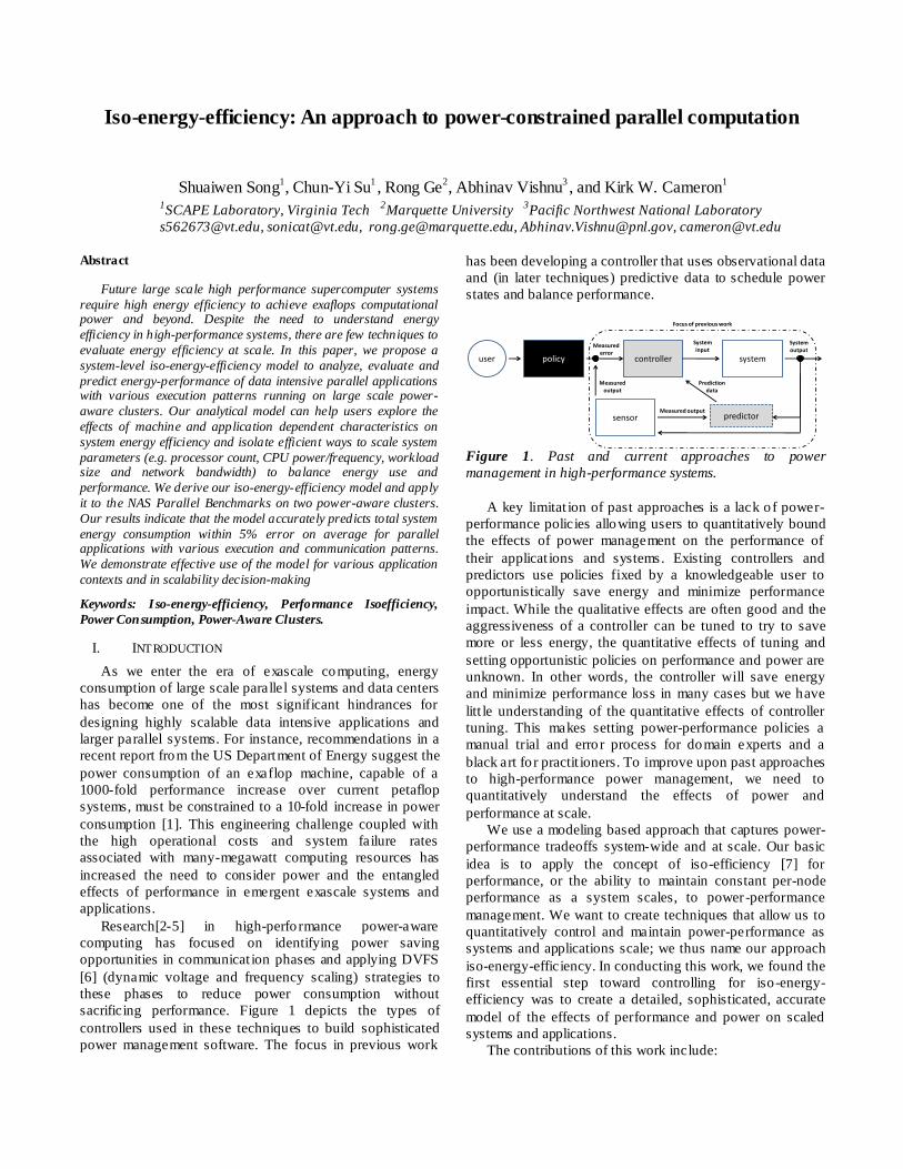
VI. MODEL DETAILED DERIVATION
In this section we describe the details for deriving the iso-
energy-efficiency model first presented in Section 3.
A. Performance Model
At the system level, the theoretical sequential execution
time for an on-chip/off-chip workload comprises three
components [35, 36]: computation time (with on-chip
instruction execution frequency), main memory access
latency , and I/O access time (with off-chip
instruction execution frequency). Thus the theoretical
execution time can be expressed as:
T= (5)
Since optimization techniques could raise various levels
of overlap between components [37], we multiply T by an
overlap factor ( ) such that:
(6)
is the actual execution time.
(GHz)
En
ergy efficien
cy

B. Energy Model for one and p parallel processor(s):
When executing a parallel applicat ion, total energy
consumption can be divided into four parts: computation
energy, main memory access energy, , I/O access
energy, , and other system components energy, ,
such as motherboard, system and CPU fans, power supply,
etc. Thus, we have total energy E [20]: E = (7)
The first three parts of this equation can be further
separated into two energy states: running state and idle state.
For example, can be divided into and . Thus,
we can deduce total energy E as [18, 20]:
(8).
From (6) and (8),
(9)
where is the total computation time; is the
total memory access time and is the total I/O access
time.
Equation (9) seems quite cumbersome; however, it is
intuitive: is the total energy consumption of
an idle-state system during an applicat ion’s execution time.
is the additional energy used while an applicat ion
is performing computation. Similarly, and
are the additional energy consumption for
conducting main memory and I/O accesses.
Figure 10. Power Profiling of MPI_FFT program in HPCC
Benchmark
Figure 10 provides additional insight to Equation (9). It
shows the power profiling of the MPI_FFT program in the
HPC Challenge Benchmark [19] measured by the
PowerPack framework. The power fluctuates for each
component over the idle-state power line (dashed line)
during the execution time. For the CPU, the red shaded
(lower) portion in Figure 10 represents total CPU energy
consumption in idle -state, and the blue (upper) portion
represents the additional energy while doing computation.
In reality, I/O access time includes the network and all
kinds of local storage devices accesses. If an application is
disk I/O-intensive, it should introduce to the
performance and the energy model. For simplicity, we
assume a simple, flat model for I/O accesses though the
benchmarks we measured did not exercise I/O making this
component effectively zero. Users can always replace
with any combinations of specific I/O components
according to their parallel applicat ions. Demonstrating the
accuracy of the model for all types of I/O is beyond the
scope of this paper and the subject of future work.
The equations follow similar to Equation (6):
(10)
With energy model:
(11)
In our experiments (on both the Dori system with
Ethernet and SystemG with InfiniBand), the difference
between is not significant so we
simply ignore the effect in (11):
(12)
C. Energy Model for A Single Processor
Equations (10) and (12) are the kernel components of the
performance model and iso-energy-efficiency model in this
paper. Let us apply these to which we discussed in
Section 3. When an application executes on a single
processor, there are no messages exchanged. This means no
in (10). Thus,
(13) where
D. Energy Model for p Parallel Processors
Similarly, to get we define the energy model in ith
( ) processor among p parallel processors:
(14)
where
In (14), and are computation and memory
access overheads for the ith of p processors in terms of
0
10
20
30
40
50
60
70
80
90
100
0.00
1.31
2.61
3.93
5.23
6.53
8.12
9.13
10.4
2
11.7
4
13.0
4
14.3
4
15.6
4
16.9
4
18.2
5
19.5
5
20.8
5
22.1
5
23.4
5
24.7
6
26.0
6
27.3
6
28.6
6
cpu mem disk motherboard
Wctc∆Pc
αT(Pc-idle )
Watts
∆Pc
Pc-idle
Secs
parallelism. Thus, we have representing total energy
consumption for all processors:
(15) where,
nd i l “ ” r r n u i n f ll
workload in all processors.
From (1) we can calcu late the energy overhead
(16)
r
In (15) and (16), is the total parallel computation
overhead ( = ) and represents the total
parallel memory access overhead ( ).
stands for accumulated networking time.
can be fu rther div ided into two parts: message
start up time and data transmitting t ime [32].
Communicat ion overhead modeling varies depending on
application and network infrastructure. Equation (17) is a
general approach and specific parameterizat ion for network
modeling is applied for each application (see Section 5).
(17)
So that can be expressed as:
E. Energy Efficiency Factor (EEF)
Using the Equations (13) and (18), we can formulate the
Energy Efficiency Factor (EEF) more accurately,
(19)
Where
)
Equation (19) contains two categories of parameters
which d irectly impact performance and energy consumption:
1) machine dependent variables
and 2) application
dependent variables: and B. For the
application dependent vector, , the processor number p
and problem size n are two main factors affecting these
parameters. They can be represented as
.
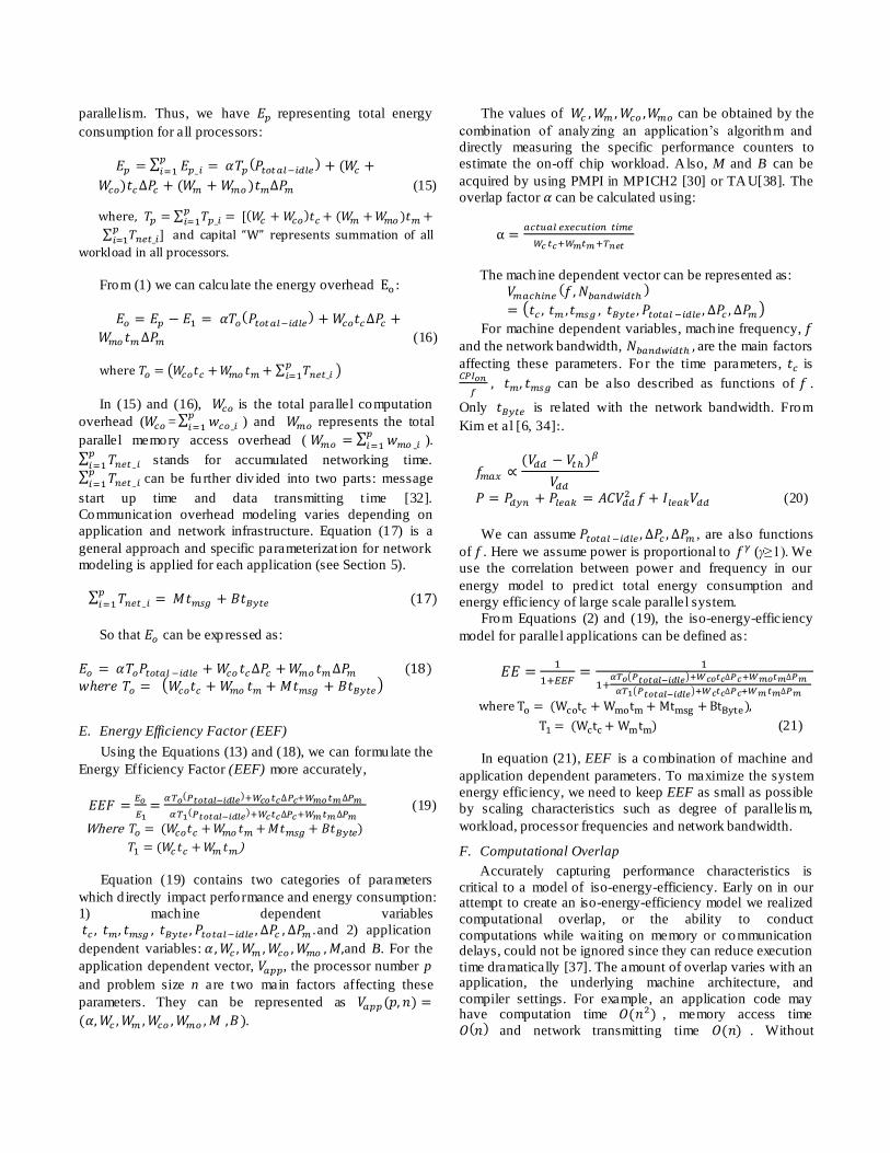
The values of can be obtained by the
combination of analyzing an application’s algorithm and
directly measuring the specific performance counters to
estimate the on-off chip workload. A lso, M and B can be
acquired by using PMPI in MPICH2 [30] or TAU[38]. The
overlap factor can be calculated using:
The machine dependent vector can be represented as:
For machine dependent variables, machine frequency,
and the network bandwidth, are the main factors
affecting these parameters. For the time parameters, is
can be also described as functions of .
Only is related with the network bandwidth. From
Kim et al [6, 34] .
(20)
We can assume , are also functions
of . Here we assume power is proportional to (γ≥1). We
use the correlation between power and frequency in our
energy model to pred ict total energy consumption and
energy efficiency of large scale parallel system.
From Equations (2) and (19), the iso-energy-efficiency
model for parallel applications can be defined as:
where ,
) (21)
In equation (21), EEF is a combination of machine and
application dependent parameters. To maximize the system
energy efficiency, we need to keep EEF as small as possible
by scaling characteristics such as degree of parallelis m,
workload, processor frequencies and network bandwidth.
F. Computational Overlap
Accurately capturing performance characteristics is
critical to a model of iso-energy-efficiency. Early on in our attempt to create an iso-energy-efficiency model we realized
computational overlap, or the ability to conduct
computations while waiting on memory or communication delays, could not be ignored since they can reduce execution
time dramatically [37]. The amount of overlap varies with an application, the underlying machine architecture, and
compiler settings. For example, an application code may have computation time , memory access time
and network transmitting time . Without

optimization, the total execution time is ;
however, the actual time is smaller. Thus we propose a comprehensive optimizat ion
parameter, α, to capture computational overlap. α Theoretical
execution time consists of computation time, memory access time, and remote data access time (or network transmission
time). Thus we have:
And we can define :
For parallel applications, we found empirically for the
applications studied that an application using the same
compiler settings has the same α value under different levels of parallelis m. However, different applications could have
different α due to different execution patterns. In addition, same applications running on different machines also have
different α values because of diverse underlying architectures.
VII. CONCLUSIONS
In this paper, we present a system level energy efficiency
model for various parallel applications and large scale parallel system architectures. We extend the concept of
performance isoefficiency to iso-energy-efficiency and show how to build an accurate system level energy efficiency
model step by step. Then we apply our analytical model to real scientific applications from NAS Parallel Benchmark
suites and illustrate how to derive essential model parameters
to predict total system energy consumption and efficiency for large scaling parallel systems. After a thorough and detailed
investigation of machine and application dependent parameters which have nontrivial impact on system energy
efficiency, we apply the model to three scientific benchmarks representing different execution patterns to
study what the influential factors are for system energy
efficiency and how to scale them to maintain efficiency. The results conducted on two power-aware clusters show that our
model can predict total system energy consumption within average 5% prediction error rate for parallel applications
with various execution and communication patterns. And also, in the case study experiments, the results clearly show
what the most influential factors are and how these factors
can be tuned to maintain energy efficiency. Though this model can precisely predict energy in various combinations
of applications and hardware architecture, we still have a bit more parameters compared with the micro-architecture
approach. In the future, we plan to integrate PowerPack with other system measurement tools and together make it more
compatible and easier for all users to model. Also, we want to extend the current model to heterogeneous systems.
REFERENCES
[1] (2010). US department of energy annual report. Available: http://www.eia.doe.gov/
[2] V. W. Freeh, F. Pan, N. Kappiah, D. K. Lowenthal, and
R. Springer, "Exploring the Energy-Time Tradeoff in
MPI Programs on a Power-Scalable Cluster," presented
at the Proceedings of the 19th IEEE International Parallel and Distributed Processing Symposium (IPDPS'05) -
Papers - Volume 01, 2005.
[3] R. Ge, X. Feng, and K. W. Cameron, "Improvement of
Power-Performance Efficiency for High-End
Computing," presented at the Proceedings of the 19th IEEE International Parallel and Distributed Processing
Symposium (IPDPS'05) - Workshop 11 - Volume 12,
2005.
[4] R. Ge, X. Feng, and K. W. Cameron, "Performance-
constrained Distributed DVS Scheduling for Scientific Applications on Power-aware Clusters," presented at the
Proceedings of the 2005 ACM/IEEE conference on
Supercomputing, 2005.
[5] V. W. Freeh and D. K. Lowenthal, "Using multiple
energy gears in MPI programs on a power-scalable cluster," presented at the Proceedings of the tenth ACM
SIGPLAN symposium on Principles and practice of
parallel programming, Chicago, IL, USA, 2005.
[6] J. Li and J. F. Martinez, "Dynamic power-performance
adaptation of parallel computation on chip multiprocessors," in The Twelfth International
Symposium on High-Performance Computer
Architecture, 2006, pp. 77-87.
[7] A. Y. Grama, A. Gupta, and V. Kumar, "Isoefficiency:
measuring the scalability of parallel algorithms and architectures," in Multiprocessor performance
measurement and evaluation, ed: IEEE Computer
Society Press, 1995, pp. 103-112.
[8] (2010). The NAS Parallel Benchmarks. Available:
http://www.nas.nasa.gov/Resources/Software [9] G.M. Amdahl, "Validity of the Single Processor
Approach to Achieving Large-Scale Computing
Capabilities," AFIPS Spring Joint Computer Conference,
Reston, VA, 1967.
[10] A. Y. Grama, A. Gupta, V. Kumar, and G. Karypis, Introduction to Parallel Computing, 2 ed.: The Addision-
Wesley Longman Publishing, 2003.
[11] J. L. Gustafson, "Reevaluating Amdahl's law," Commun.
ACM, vol. 31, pp. 532-533, 1988.
[12] X.-H. Sun and L. M. Ni, "Scalable problems and memory-bounded speedup," J. Parallel Distrib. Comput.,
vol. 19, pp. 27-37, 1993.
[13] M. D. Hill and M. R. Marty, "Amdahl's law in the
multicore era," IEEE Computer, 2008.
[14] J. M. Paul and B. H. Meyer, "Amdahl's law revisited for single chip systems," Int. J. Parallel Program., vol. 35, pp.
101-123, 2007.
[15] (2010). "TOP500 Supercomputing Sites". Available:
http://www.top500.org
[16] W. Feng and K.Cameron, "The Green500 List: Encouraging Sustainable Supercomputing" Computer,
vol. 40, p. 50_55, 2007.
[17] (2008). The SPEC Power benchmark. Available:
http://www.spec.org/power_ssj2008/

[18] S. Song, R. Ge, X. Feng, and K. W. Cameron, "Energy
Profiling and Analysis of the HPC Challenge
Benchmarks," International Journal of High Performance Computing Applications, vol. 23, pp. 265-276, 2009.
[19] P. R. Luszczek, D. H. Bailey, J. J. Dongarra, J. Kepner,
R. F. Lucas, R. Rabenseifner, et al., "The HPC Challenge
(HPCC) benchmark suite," presented at the Proceedings
of the 2006 ACM/IEEE conference on Supercomputing, Tampa, Florida, 2006.
[20] R. Ge, X. Feng, S. Song, and K. W. Cameron,
"PowerPack: Energy Profiling and Analysis of High-
Performance Systems and Applications," IEEE
Transactions on Parallel and Distributed Systems, vol. 99, pp. 658-671, 2009.
[21] K. W. Cameron, R. Ge, and X. Feng, "High-Performance,
Power-Aware Distributed Computing for Scientific
Applications," Computer, vol. 38, pp. 40-47, 2005.
[22] X. Feng, R. Ge, and K. W. Cameron, "Power and Energy Profiling of Scientific Applications on Distributed
Systems," presented at the Proceedings of the 19th IEEE
International Parallel and Distributed Processing
Symposium (IPDPS'05) - Papers - Volume 01, 2005.
[23] R. Springer, D. K. Lowenthal, B. Rountree, and V. W. Freeh, "Minimizing execution time in MPI programs on
an energy-constrained, power-scalable cluster,"
presented at the Proceedings of the eleventh ACM
SIGPLAN symposium on Principles and practice of
parallel programming, New York, New York, USA, 2006.
[24] V. W. Freeh and D. K. Lowenthal, "Using multiple
energy gears in MPI programs on a power-scalable
cluster," presented at the Proceedings of the tenth ACM
SIGPLAN symposium on Principles and practice of parallel programming, Chicago, IL, USA, 2005.
[25] R. Ge and K. W. Cameron, "Power-Aware Speedup," in
proceedings of the 21st IEEE International Parallel and
Distributed Processing Symposium, 2007, pp. 56-56.
[26] N. Jiang, J. Pisharath, and A. Choudhary, "Characterizing and improving energy-delay tradeoffs in
heterogeneous communication systems," Signals,
Circuits and Systems, 2003. SCS 2003. International
Symposium vol. 2, pp. 409-412, 2003.
[27] Y. Ding, K. Malkowski, P. Raghavan, and M. Kandemir, "Towards Energy Efficient Scaling of Scientific Codes,"
in IEEE International Symposium on Parallel and
Distributed Processing, 2008, pp. 1 - 8
[28] D. A. Patterson and J.L.Hennessy, Computer
Architecture: A quantitative approach, 3rd ed. San Francisco, CA: Morgan Kaufmann Publishers, 2003.
[29] (2010). LMbench - Tools for Performance Analysis.
Available: http://www.bitmover.com/lmbench/
[30] MPICH2: high-performance and widely portable
implementation of the Message Passing Interface (MPI) standard. Available:
http://phase.hpcc.jp/mirrors/mpi/mpich2/
[31] InfiniBand Trade Association. Available:
http://www.infinibandta.org/
[32] J. Pjeivac-Grbovi, T. Angskun, G. Bosilca, G. E. Fagg, E. Gabriel, and J. J. Dongarra, "Performance analysis of
MPI collective operations," Cluster Computing, vol. 10,
pp. 127-143, 2007.
[33] R. Thakur, "Improving the performance of collective
operations in MPICH," in Recent Advances in Parallel
Virtual Machine and Message Passing Interface. Number 2840 in LNCS, ed: Springer Verlag, 2003, pp. 257–267.
[34] N. S. Kim, T. Austin, D. Blaauw, T. Mudge, Kriszti, n.
Flautner, et al., "Leakage Current: Moore's Law Meets
Static Power," Computer, vol. 36, pp. 68-75, 2003.
[35] K. Choi, R. Soma, and M. Pedram, "Dynamic voltage and frequency scaling based on workload
decomposition," presented at the Proceedings of the
2004 international symposium on Low power electronics
and design, Newport Beach, California, USA, 2004.
[36] Q. Wu, M. Martonosi, D. W. Clark, V. J. Reddi, D. Connors, Y. Wu, et al., "A Dynamic Compilation
Framework for Controlling Microprocessor Energy and
Performance," presented at the Proceedings of the 38th
annual IEEE/ACM International Symposium on
Microarchitecture, Barcelona, Spain, 2005. [37] K. C. Louden, Compiler Construction: Principles and
Practice, 1st edition, 997.
[38] (2010). TAU: Tuning and Analysis Utilities. Available:
http://www.cs.uoregon.edu/research/tau/home.php