ISSN 2167-1273 Volume 1 Issue 9 October FEA Information Engineering Journal Information Engineering Journal... · Issue 9 . October. FEA Information Engineering Journal SIMULATION

ISSN 2167-1273 Volume 1

Issue 9 October

FEA Information Engineering Journal

SIMULATION

2 Fea Information Engineering Journal September 2012


Aim and Scope FEA Information Engineering Journal (FEAIEJ™) is a monthly published online journal to cover the latest Finite Element Analysis Technologies. The journal aims to cover previous noteworthy published papers and original papers. All published papers are peer reviewed in the respective FEA engineering fields. Consideration is given to all aspects of technically excellent written information without limitation on length. All submissions must follow guidelines for publishing a paper, or periodical. If a paper has been previously published, FEAIEJ requires written permission to reprint, with the proper acknowledgement give to the publisher of the published work. Reproduction in whole, or part, without the express written permissio of FEA Information Engineering Journal, or the owner of of the copyright work, is strictly prohibited. FEAIJ welcomes unsolicited topics, ideas, and articles. Monthly publication is limited to no more then five papers, either reprint, or original. Papers will be archived on www.feaiej.com For information on publishing a paper original or reprint contact [email protected] Subject line: Journal Publication

Cover: Figure 1. PLEX a) model geometry b) model mesh (flesh is transparent) A Finite Element Model of the Pelvis and Lower Limb for Automotie Impact Applications

http://www.feaiej.com/

mailto:[email protected]

3 Fea Information Engineering Journal September 2012


TABLE OF CONTENTS

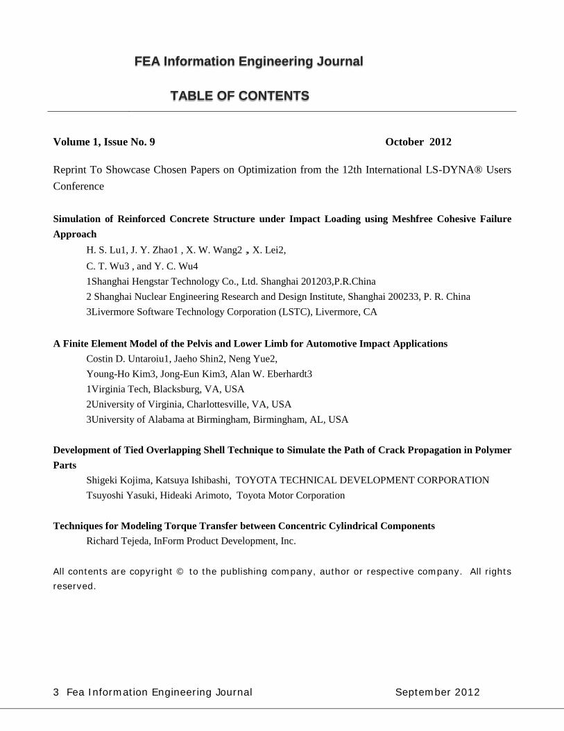
Volume 1, Issue No. 9 October 2012 Reprint To Showcase Chosen Papers on Optimization from the 12th International LS-DYNA® Users Conference Simulation of Reinforced Concrete Structure under Impact Loading using Meshfree Cohesive Failure Approach

H. S. Lu1, J. Y. Zhao1 , X. W. Wang2，X. Lei2, C. T. Wu3 , and Y. C. Wu4 1Shanghai Hengstar Technology Co., Ltd. Shanghai 201203,P.R.China 2 Shanghai Nuclear Engineering Research and Design Institute, Shanghai 200233, P. R. China 3Livermore Software Technology Corporation (LSTC), Livermore, CA

A Finite Element Model of the Pelvis and Lower Limb for Automotive Impact Applications Costin D. Untaroiu1, Jaeho Shin2, Neng Yue2, Young-Ho Kim3, Jong-Eun Kim3, Alan W. Eberhardt3 1Virginia Tech, Blacksburg, VA, USA 2University of Virginia, Charlottesville, VA, USA 3University of Alabama at Birmingham, Birmingham, AL, USA

Development of Tied Overlapping Shell Technique to Simulate the Path of Crack Propagation in Polymer Parts

Shigeki Kojima, Katsuya Ishibashi, TOYOTA TECHNICAL DEVELOPMENT CORPORATION Tsuyoshi Yasuki, Hideaki Arimoto, Toyota Motor Corporation

Techniques for Modeling Torque Transfer between Concentric Cylindrical Components Richard Tejeda, InForm Product Development, Inc.

All contents are copyright © to the publishing company, author or respective company. All rights

reserved.

12th

International LS-DYNA® Users Conference Simulation(1)

1

Simulation of Reinforced Concrete Structure under Impact

Loading using Meshfree Cohesive Failure Approach

H. S. Lu1, J. Y. Zhao1 , X. W. Wang2，X. Lei2, C. T. Wu3 , and Y. C. Wu4

1Shanghai Hengstar Technology Co., Ltd. Shanghai 201203,P.R.China

2 Shanghai Nuclear Engineering Research and Design Institute, Shanghai 200233, P. R. China

3Livermore Software Technology Corporation (LSTC), Livermore, CA 94551,USA

4Karagozian & Case, Burbank, CA 91505,USA

Abstract

Reliable numerical simulation of failure is important for the design and planning of new solids and structures, as well as for the safety assessment of existing ones. In the past two decades, gradient and non-local models for regularizing loss of ellipticity due to material failure using non-standard finite element method and more recently the meshfree method have been the topic of considerable research. Alternatively, discontinuous partition of unity enrichments and meshfree visibility concepts were proposed and used in finite element method (also called extended finite element method - XFEM) and meshfree method to model cracks. Due to the fact that the description of crack plane in XFEM using level set method still presents several difficulties in the three-dimensional simulation of solids, the meshfree method using visibility concept is tested for the solid failure analysis of reinforced concrete structure under impact loading. The current method incorporates the discontinuous field into the generalized meshfree approximation [1] by the introduction of visibility approach [2]. To determine the onset of fracture and subsequently the crack propagation, a stress-based initial-rigid cohesive cracking model was developed for the brittle and semi-brittle materials. After the insertion of new crack, the state variables are interpolated and transferred to the new stress point using second-order meshfree approximation [3]. To integrate the discrete equations involving the crack plane, the strain smoothing algorithm developed in SCNI method [4] was adopted in this development. A typical reinforced concrete structure under impact loading failure involving multi-cracks is modeled using the developed method and results are presented.

Generalized Meshfree Approximation The generalized meshfree (GMF) approximation method can be used to construct a convex, non-convex, or combined convex and non-convex approximation for meshfree computation. The GMF approximation has one unique feature. That is it naturally bears the weak Kronecker-delta property at boundaries regardless of its convexity or non-convexity. This property makes the imposition of essential boundary conditions in meshfree methods easier. The first-order GMF approximation in one dimension is described as follows:

Simulation(1) 12th

International LS-DYNA® Users Conference

2

1

(x; ) ( , )(x, )(x; ) ( , )

i a i i ii n

a j j jj

X XX X

for fixed x , (1)

subjected to

1(x) 0

n

i ii

R X

(linear constraints), (2)

where (x; ) ( , )i a i i iX X , (3)

1 1

(x; ) ( , )n ni a i i ii i

X X

. (4) In the GMF approximation, the property of the partition of unity is automatically satisfied by the normalization in Eq. (1). The completion of the GMF approximation is achieved by finding to satisfy Eq. (2). To determine at any fixed x in Eq. (1), a root-finding algorithm is required for the non-linear base functions. The spatial derivative of the GMF approximation is given by

,x , ,xi

i iddx

, (5)

where ,x,x,x

1

nji

i ij

, (6)

,x ,x ,xi a i a i , (7)

,,,

1

na ja i

i ij

, (8)

1,x ,xJ R , (9)

,,

1 1

n na ja i

ii j

J X R

, (10)

,x ,x1

1n

i ii

R X

. (11)

By choosing appropriate basis functions in the GMF approximation, some well-known convex or non-convex approximations, such as Shephard, Moving-least-squared (MLS), Reproducing kernel (RK) and Maximum entropy (ME) approximations, can be recovered. When the basis function is non-positive such as polynomials, the convex approximation property and Kronecker-delta property at the boundaries are lost and a boundary correction function [1] has to be introduced to achieve the local convexity at the boundary nodes. The MLS and RK approximations are the typical non-convex approximations. In the MLS or the RK approximation, polynomial basis functions are introduced to meet the polynomial reproducing conditions. As in the ME approximation, the employment of exponential basis function takes into account the exponential distribution of the probability at the node in the view point of the information theory. Therefore it yields a convexity in the approximation since the exponential function is non-negative. It is noted that other probability density function can

12th


3

also be chosen as a basis function and different entropy measure can also be used to obtain the convex approximation. The enriched basis function and weight function play an important role in controlling the smoothness and convexity of the approximation. The coefficient in Eq. (1) can be viewed as a corrected weight to impose polynomial reproducibility. Table 1 gives the typical basis functions used to generate the convex and non-convex GMF approximations. In this study, the GMF(tanh) approximation is adopted for the simulation.

Table 1. Examples of basis functions in the GMF approximations

Convexity Basis function Abbreviation Note

Convex approximation

xe GMF(exp) ME Approximation (Shannon entropy)

1+tanh(x) GMF(tanh) New approximation

-121+ tan (x)π

GMF(atan) New approximation

1-11-1+ x

(Renyi basis function)

GMF(Renyi)

ME Approximation (Renyi entropy) 0.5 1.0

Non-convex approximation

MLS approximation ( 2 )

1+ x GMF(MLS) MLS approximation

1+ x3 GMF(x3) New approximation

ex(1+ x3) GMF(exp·x3) New approximation

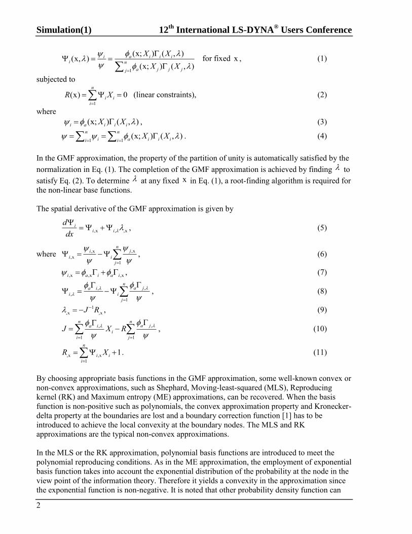
Review of K&C Concrete Model (*MAT_72） The Release III KCC model was made available in LS-DYNA in 2004. The model has been extensively verified in both dynamic and quasi – static load environments [5, 6, 7]. To verify the basic capabilities of the KCC model, several single element numerical results are included herein. Figure 1 shows the stress – strain relationship for a single element UUC test. It is seen that a yield point is reached first, then very limited hardening undergoes, and finally, strain softening phenomenon is observed. It should be pointed out that, in the Figure, positive volumetric strain corresponds to volume compaction and negative volumetric strain corresponds to volume expansion. As a consequence, it can be concluded that the shear dilation effect is captured by the material model properly, since the concrete is compacted early on and after it reaches its peak strength, the concrete is expanded.

Simulation(1) 12th


4

Figure 1 Single element UUC test

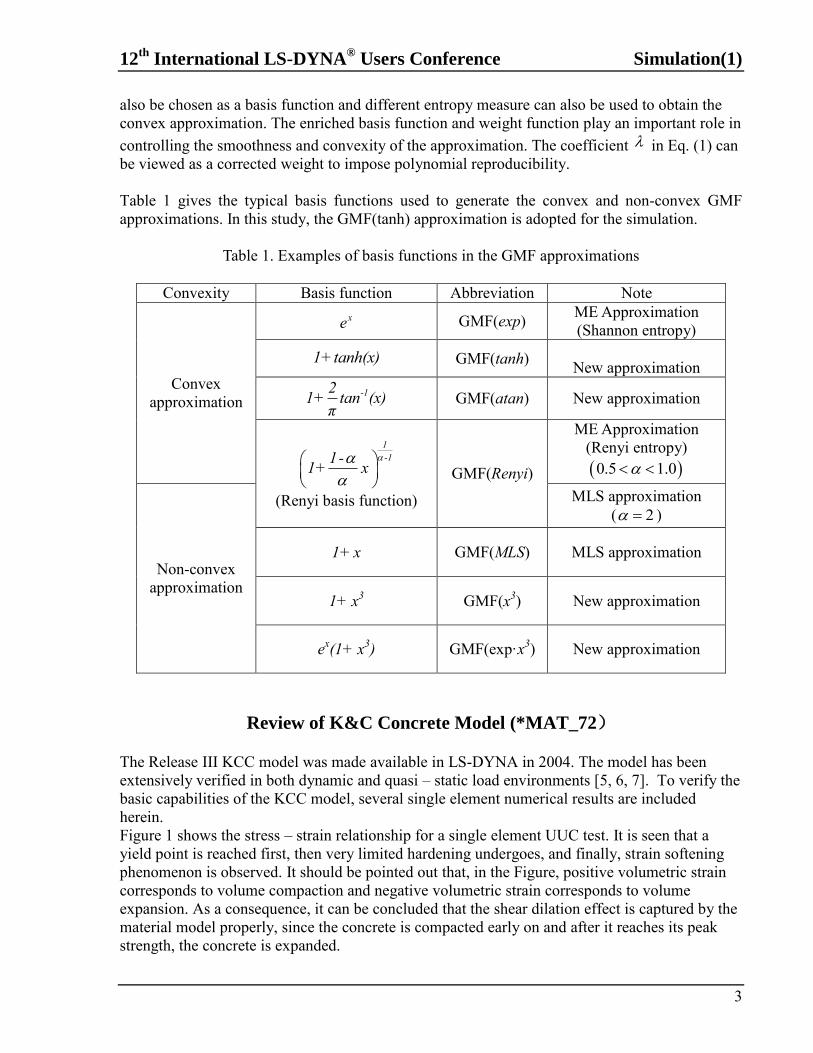
Figure 2 shows the stress – strain relationships for single element triaxial compression (TXC) tests, where solid line represents axial strain axial stress relationships, dotted lines represent lateral strain – axial stress relationships, and legend indicates confinement pressure.Several conclusions can be made from these tests. First, confinement effect is captured properly by the material model since concrete strength is observed much higher than its unconfined compressive strength (41.4 MPa). Second, the brittle – ductile transition under confinements is modeled properly. It is seen that strain softening behavior occurs when confinement pressure is low, and the concrete behaves elastic – hardening plastically, just like metal, when confinement pressure is very high.

Figure 2 Single element TXC tests

Modified Cohesive Zone Model

12th


5

In meshfree cohesive failure approach, a modified cohesive zone model [8] is utilized to describe the material failure of concrete in tension mode in addition to the concrete model described

previously. The effective traction ( efsT ) and the effective crack opening displacement ( efs ) are defined as

2 22

1efs n tT T T

, and (12)

2 2 2efs n t (13)

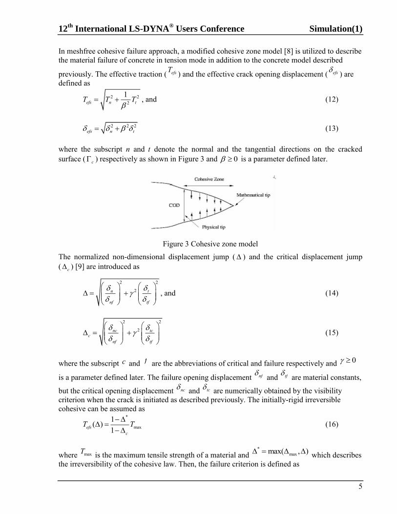
where the subscript n and t denote the normal and the tangential directions on the cracked surface ( c ) respectively as shown in Figure 3 and 0 is a parameter defined later.

Figure 3 Cohesive zone model

The normalized non-dimensional displacement jump ( ) and the critical displacement jump ( c ) [9] are introduced as

2 2

2n t

nf tf

, and (14)

2 2

2nc tcc

nf tf

(15)

where the subscript c and f are the abbreviations of critical and failure respectively and 0

is a parameter defined later. The failure opening displacement nf and tf are material constants,

but the critical opening displacement nc and tc are numerically obtained by the visibility criterion when the crack is initiated as described previously. The initially-rigid irreversible cohesive can be assumed as

*

max1( )1efs

c

T T

(16)

where maxT is the maximum tensile strength of a material and *

maxmax( , ) which describes the irreversibility of the cohesive law. Then, the failure criterion is defined as

Simulation(1) 12th


6

max( ) 0efsT T (17)

which is the traction-driven failure criterion. Originally, the initially-rigid cohesive law was proposed with the interface elements in the FE framework. In the FE framework, the crack initiation and propagation are occurred at nodes on the boundaries of elements. Hence, the critical opening displacement is always zero. However, in the meshfree method, the visibility criterion produces the positive non-zero critical opening displacement when the crack is initiated. Therefore, after the crack is initiated, the initially-elastic irreversible cohesive law with the critical opening displacement is adopted for the softening stage. This is the combined initially-rigid and initially-elastic irreversible cohesive law or the hybrid irreversible cohesive law. In other word, the initially-rigid cohesive law is used for the crack initiation and then it is switched to the initially-elastic irreversible cohesive law until the crack is separated completely. The initially-elastic irreversible cohesive laws of the normal and the tangential tractions can be defined as

*

( )efs nn

nf

TT

, and (18)

*

( )efs tt

tf

TT

(19)

where 0 is a parameter defined later. In the formulations above, there are three parameters, , and . The relationship among those parameters can be found. By inserting Eq. (18) and (19) into Eq. (16) at

ct t , then Eq. (16) becomes

2 22( )efs nc tc

efsc nf tf

TT

. (20)

Obviously, the square root term in Eq. (20) should become c and is equal to Eq. (15). Then, we obtain

. (21)

By dividing Eq. (13) by nf , then Eq. (13) becomes

2 2 2

2efs tfn t

nf nf nf tf

. (22)

Let efs

nf

, using Eq. (14) and Eq. (21), we have

12th


7

2 tf

nf

. (23)

Numerical Example

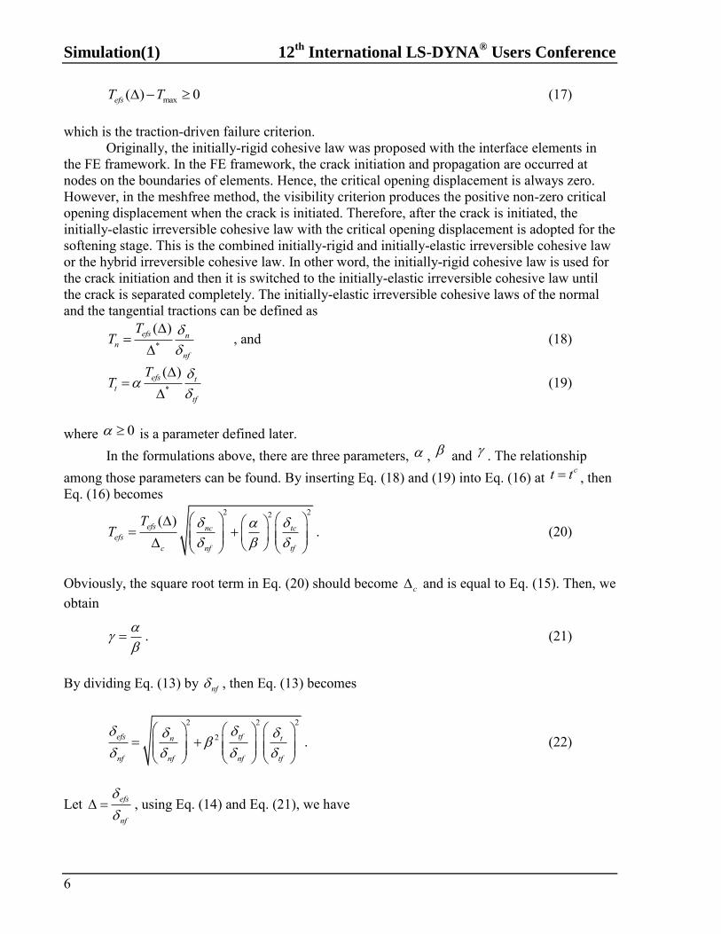
A reinforced concrete structure under impact loading is analyzed with using meshfree cohesive failure approach. As in figure 3(a) and (b), the impactor is modeled such that the mass and strength distribution in the impact direction are corresponded to that of the scaled aircraft model. The thickness of RC panel is 6 cm, and the outer layer of panel is fixed. Reinforcement ration is 0.47% with D3 rebar. The concrete compressive strength is 31.4 N/mm^2. The common nodes are used to model the rebar coupled to the concrete. In case of cohesive failure, only mode I

failure is considered. The maximum tensile strength maxT is taken to be 2.9 MPa and the critical

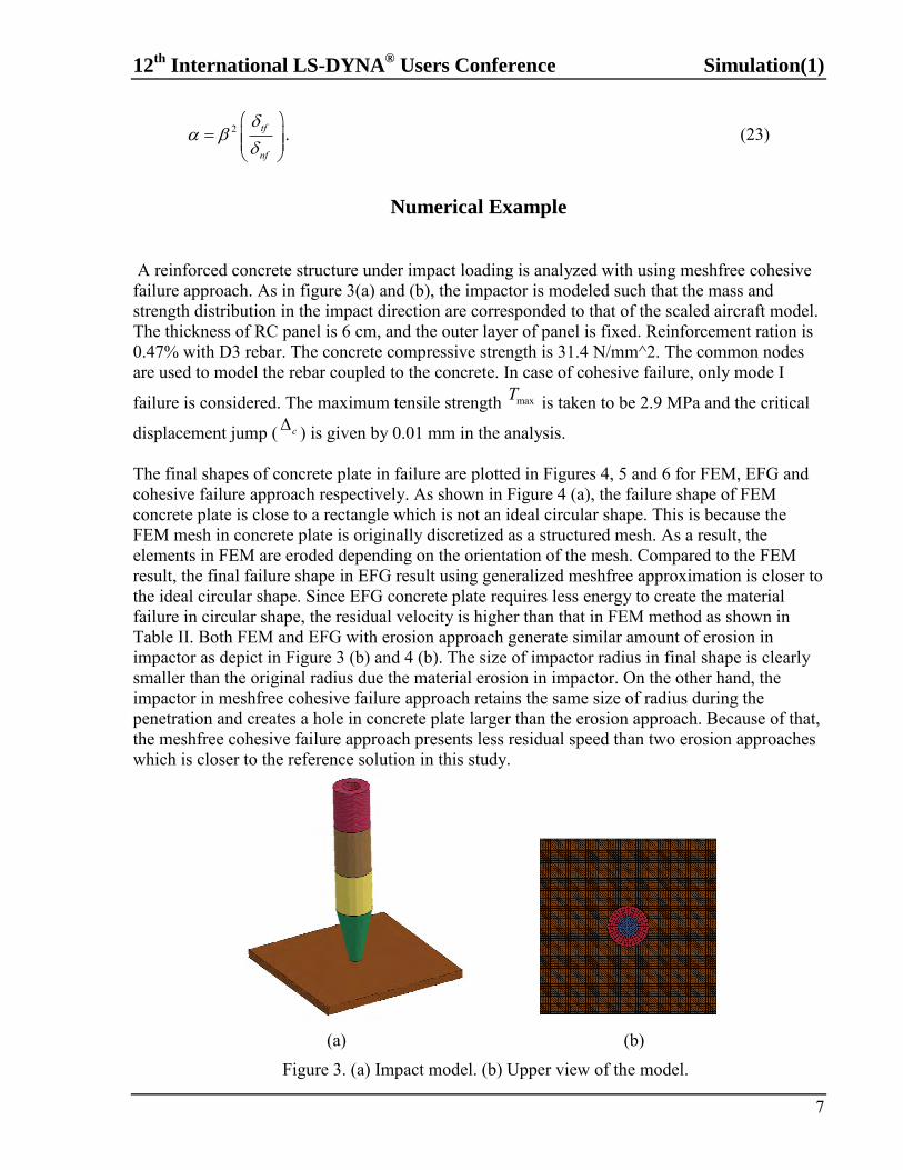
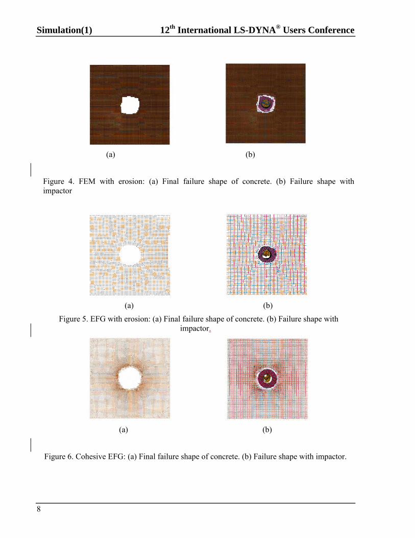
displacement jump ( c ) is given by 0.01 mm in the analysis. The final shapes of concrete plate in failure are plotted in Figures 4, 5 and 6 for FEM, EFG and cohesive failure approach respectively. As shown in Figure 4 (a), the failure shape of FEM concrete plate is close to a rectangle which is not an ideal circular shape. This is because the FEM mesh in concrete plate is originally discretized as a structured mesh. As a result, the elements in FEM are eroded depending on the orientation of the mesh. Compared to the FEM result, the final failure shape in EFG result using generalized meshfree approximation is closer to the ideal circular shape. Since EFG concrete plate requires less energy to create the material failure in circular shape, the residual velocity is higher than that in FEM method as shown in Table II. Both FEM and EFG with erosion approach generate similar amount of erosion in impactor as depict in Figure 3 (b) and 4 (b). The size of impactor radius in final shape is clearly smaller than the original radius due the material erosion in impactor. On the other hand, the impactor in meshfree cohesive failure approach retains the same size of radius during the penetration and creates a hole in concrete plate larger than the erosion approach. Because of that, the meshfree cohesive failure approach presents less residual speed than two erosion approaches which is closer to the reference solution in this study.

(a) (b)

Figure 3. (a) Impact model. (b) Upper view of the model.

Simulation(1) 12th


8

(a) (b)

Figure 4. FEM with erosion: (a) Final failure shape of concrete. (b) Failure shape with impactor

(a) (b)

Figure 5. EFG with erosion: (a) Final failure shape of concrete. (b) Failure shape with impactor.

(a) (b)

Figure 6. Cohesive EFG: (a) Final failure shape of concrete. (b) Failure shape with impactor.

12th


9

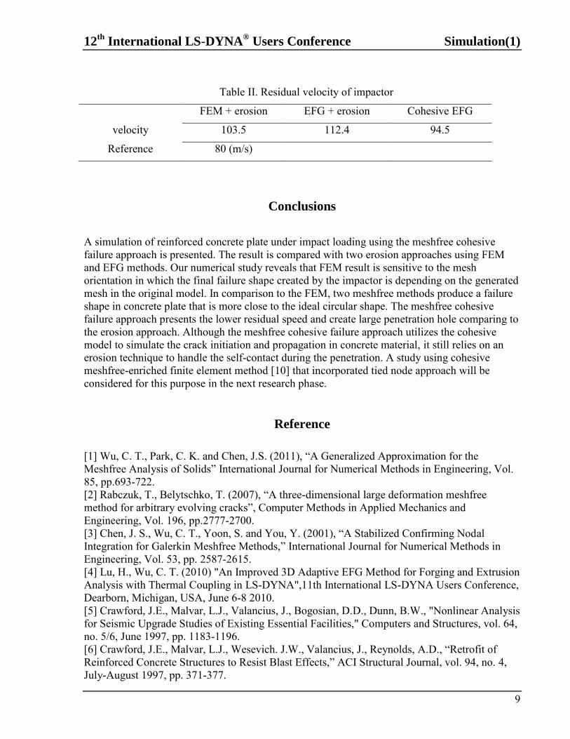
Table II. Residual velocity of impactor

FEM + erosion EFG + erosion Cohesive EFG

velocity 103.5 112.4 94.5

Reference 80 (m/s)

Conclusions

A simulation of reinforced concrete plate under impact loading using the meshfree cohesive failure approach is presented. The result is compared with two erosion approaches using FEM and EFG methods. Our numerical study reveals that FEM result is sensitive to the mesh orientation in which the final failure shape created by the impactor is depending on the generated mesh in the original model. In comparison to the FEM, two meshfree methods produce a failure shape in concrete plate that is more close to the ideal circular shape. The meshfree cohesive failure approach presents the lower residual speed and create large penetration hole comparing to the erosion approach. Although the meshfree cohesive failure approach utilizes the cohesive model to simulate the crack initiation and propagation in concrete material, it still relies on an erosion technique to handle the self-contact during the penetration. A study using cohesive meshfree-enriched finite element method [10] that incorporated tied node approach will be considered for this purpose in the next research phase.

Reference

[1] Wu, C. T., Park, C. K. and Chen, J.S. (2011), “A Generalized Approximation for the Meshfree Analysis of Solids” International Journal for Numerical Methods in Engineering, Vol. 85, pp.693-722. [2] Rabczuk, T., Belytschko, T. (2007), “A three-dimensional large deformation meshfree method for arbitrary evolving cracks”, Computer Methods in Applied Mechanics and Engineering, Vol. 196, pp.2777-2700. [3] Chen, J. S., Wu, C. T., Yoon, S. and You, Y. (2001), “A Stabilized Confirming Nodal Integration for Galerkin Meshfree Methods,” International Journal for Numerical Methods in Engineering, Vol. 53, pp. 2587-2615. [4] Lu, H., Wu, C. T. (2010) "An Improved 3D Adaptive EFG Method for Forging and Extrusion Analysis with Thermal Coupling in LS-DYNA",11th International LS-DYNA Users Conference, Dearborn, Michigan, USA, June 6-8 2010. [5] Crawford, J.E., Malvar, L.J., Valancius, J., Bogosian, D.D., Dunn, B.W., "Nonlinear Analysis for Seismic Upgrade Studies of Existing Essential Facilities," Computers and Structures, vol. 64, no. 5/6, June 1997, pp. 1183-1196. [6] Crawford, J.E., Malvar, L.J., Wesevich. J.W., Valancius, J., Reynolds, A.D., “Retrofit of Reinforced Concrete Structures to Resist Blast Effects,” ACI Structural Journal, vol. 94, no. 4, July-August 1997, pp. 371-377.

Simulation(1) 12th


10

[7] Crawford, J.E., Magallanes, J.M., Lan, S., and Wu, Y. “User’s manual and documentation for release III of the K&C concrete material model in LS-DYNA,” TR-11-36-1, technical report, Karagozian& Case, Burbank, CA, November, 2011. [8] Park, C. K. (2009) The development of a generalized meshfree approximation for solid and fracture analysis, Dissertation, The George Washington University. [9] Espinosa, H.D. (2003) “A grain level model for the study of failure initation and evolution in polycrystalline materials. Part I: Theory and numerical implementation”, Mechanics of Materials, vol. 35, no. 3-6, pp. 336-364. [10] Wu C. T. and Hu, W. (2011), “Meshfree-enriched simplex elements with strain smoothing for the finite element analysis of compressible and nearly incompressible solids”, Computer Methods in Applied Mechanics and Engineering, vol. 200, pp. 2991-3010.

12th


1

A Finite Element Model of the Pelvis and Lower Limb for

Automotive Impact Applications

Costin D. Untaroiu1, Jaeho Shin2, Neng Yue2, Young-Ho Kim3, Jong-Eun Kim3, Alan W. Eberhardt3

1Virginia Tech, Blacksburg, VA, USA 2University of Virginia, Charlottesville, VA, USA

3University of Alabama at Birmingham, Birmingham, AL, USA

Abstract

A finite element (FE) model of the pelvis and lower limb was developed to improve understanding of injury mechanisms of the lower extremities during vehicle collisions and to aid in the design of injury countermeasures. The FE model was developed based on the reconstructed geometry of a male volunteer close to the anthropometry of a 50th percentile male and a commercial anatomical database. The model has more than 625,000 elements included in 285 distinct components (parts). The material and structural properties were selected based on a synthesis of current knowledge of the constitutive models for each tissue. The model was validated in seventeen loading conditions observed in frontal and side impact vehicle collisions. These validations include combined axial compression and bending (mid-shaft femur, distal third leg), compression/flexion/xversion/axial rotation (foot), and lateral loading (pelvis). In addition to very good predictions in terms of biomechanical response and injuries, the model showed stability at different severe loading conditions. Overall results obtained in the validation indicated improved biofidelity relative to previous FE models. The model may be used in future for improving the current injury criteria of lower extremity and anthropometric test devices. Furthermore, the present pelvis and lower limb was coupled together with other body region FE models into the state-of-art human FE model to be used in the field of automotive safety.

Introduction

Occupant pelvis-lower extremity (PLEX) injuries in automotive crashes account for 26% of

AIS 2+ injuries for belted passengers (Morgan et al. 1990). 55% of these injuries occur in the Knee-Thigh-Hip (KTH) complex and account for 42% of the life-years lost to injury for occupants in airbag equipped vehicles (Kuppa et al. 2001). To develop a better understanding of Crash-Induced Injuries (CIIs) required in designing injury countermeasures, several experimental and numerical approaches have been used (Crandall et al. 2011). Experimental approaches have been tried to replicate CIIs in lab conditions using Post Mortem Human Subjects (PMHS) impact tests. However, understanding the injury mechanisms and development of accurate Injury Criteria using this test data is challenging due to inherent variations in terms of PMHS anthropometry and material properties. With recent rapid increases in computational power, several human numerical models have been used for vehicle safety research and development. The human finite element (FE) models are currently the most sophisticated human numerical

Simulation(1) 12th


2

models, which can provide general kinematics of the whole human body model and calculate the detailed stress/strain distributions which can be correlated with the risk of injuries.

While several FE PLEX models have been developed to investigate traffic accidents involving occupants in vehicles and pedestrians, limitations arise from their geometries, the modeling approaches used to represent their components, and limited test data used for model validation. In some models, the whole lower limb geometry or some of their components were obtained by uniformly scaling the geometry of the Visible Human dataset (Silvestri et al. 2009, Kim et al. 2005). This approach introduced inherently some local inaccuracies of the model. In other models (e.g. Huang et al. 2001, Beillas et al. 2001, Silvestri et al. 2009), the geometry of ligaments and thicker layers of cortical bone were simplified by modeling those components as bar and shell elements, respectively. Finally, all previous models could not benefit from the huge amount of material and component test data published recently.

The objective of this study was to develop a more biofidelic occupant PLEX FE model using the geometry directly reconstructed from the medical scan data of a 50th percentile male volunteer.

Methods Model Development

The geometry reconstruction of the occupant LEX was conducted by the Center for

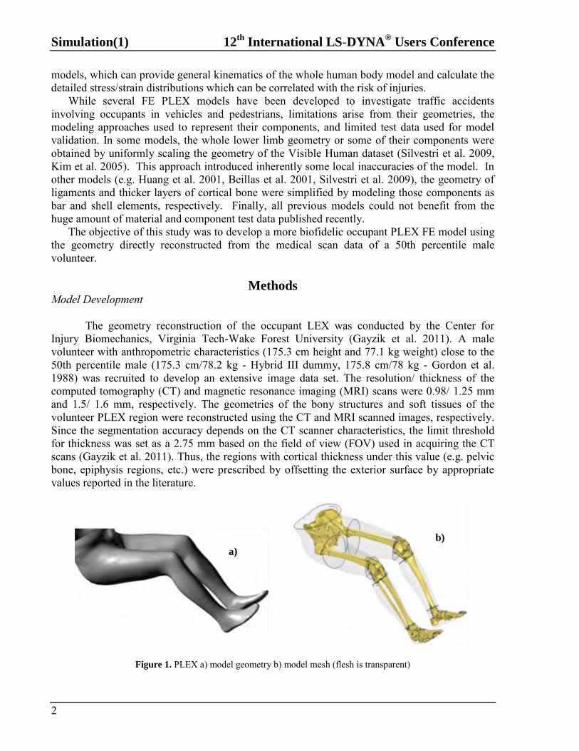
Injury Biomechanics, Virginia Tech-Wake Forest University (Gayzik et al. 2011). A male volunteer with anthropometric characteristics (175.3 cm height and 77.1 kg weight) close to the 50th percentile male (175.3 cm/78.2 kg - Hybrid III dummy, 175.8 cm/78 kg - Gordon et al. 1988) was recruited to develop an extensive image data set. The resolution/ thickness of the computed tomography (CT) and magnetic resonance imaging (MRI) scans were 0.98/ 1.25 mm and 1.5/ 1.6 mm, respectively. The geometries of the bony structures and soft tissues of the volunteer PLEX region were reconstructed using the CT and MRI scanned images, respectively. Since the segmentation accuracy depends on the CT scanner characteristics, the limit threshold for thickness was set as a 2.75 mm based on the field of view (FOV) used in acquiring the CT scans (Gayzik et al. 2011). Thus, the regions with cortical thickness under this value (e.g. pelvic bone, epiphysis regions, etc.) were prescribed by offsetting the exterior surface by appropriate values reported in the literature.

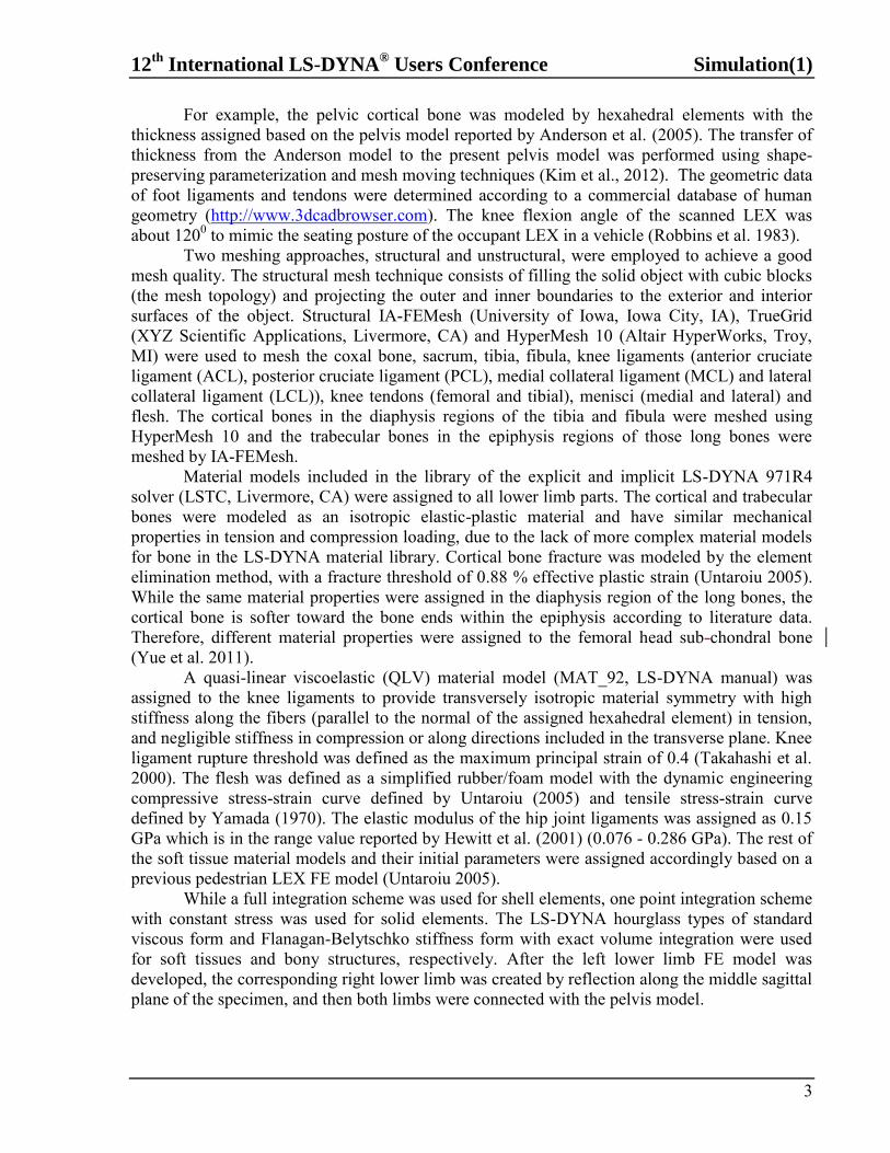
Figure 1. PLEX a) model geometry b) model mesh (flesh is transparent)

a) b)

12th


3

For example, the pelvic cortical bone was modeled by hexahedral elements with the thickness assigned based on the pelvis model reported by Anderson et al. (2005). The transfer of thickness from the Anderson model to the present pelvis model was performed using shape-preserving parameterization and mesh moving techniques (Kim et al., 2012). The geometric data of foot ligaments and tendons were determined according to a commercial database of human geometry (http://www.3dcadbrowser.com). The knee flexion angle of the scanned LEX was about 1200 to mimic the seating posture of the occupant LEX in a vehicle (Robbins et al. 1983).

Two meshing approaches, structural and unstructural, were employed to achieve a good mesh quality. The structural mesh technique consists of filling the solid object with cubic blocks (the mesh topology) and projecting the outer and inner boundaries to the exterior and interior surfaces of the object. Structural IA-FEMesh (University of Iowa, Iowa City, IA), TrueGrid (XYZ Scientific Applications, Livermore, CA) and HyperMesh 10 (Altair HyperWorks, Troy, MI) were used to mesh the coxal bone, sacrum, tibia, fibula, knee ligaments (anterior cruciate ligament (ACL), posterior cruciate ligament (PCL), medial collateral ligament (MCL) and lateral collateral ligament (LCL)), knee tendons (femoral and tibial), menisci (medial and lateral) and flesh. The cortical bones in the diaphysis regions of the tibia and fibula were meshed using HyperMesh 10 and the trabecular bones in the epiphysis regions of those long bones were meshed by IA-FEMesh.

Material models included in the library of the explicit and implicit LS-DYNA 971R4 solver (LSTC, Livermore, CA) were assigned to all lower limb parts. The cortical and trabecular bones were modeled as an isotropic elastic-plastic material and have similar mechanical properties in tension and compression loading, due to the lack of more complex material models for bone in the LS-DYNA material library. Cortical bone fracture was modeled by the element elimination method, with a fracture threshold of 0.88 % effective plastic strain (Untaroiu 2005). While the same material properties were assigned in the diaphysis region of the long bones, the cortical bone is softer toward the bone ends within the epiphysis according to literature data. Therefore, different material properties were assigned to the femoral head sub-chondral bone (Yue et al. 2011).

A quasi-linear viscoelastic (QLV) material model (MAT_92, LS-DYNA manual) was assigned to the knee ligaments to provide transversely isotropic material symmetry with high stiffness along the fibers (parallel to the normal of the assigned hexahedral element) in tension, and negligible stiffness in compression or along directions included in the transverse plane. Knee ligament rupture threshold was defined as the maximum principal strain of 0.4 (Takahashi et al. 2000). The flesh was defined as a simplified rubber/foam model with the dynamic engineering compressive stress-strain curve defined by Untaroiu (2005) and tensile stress-strain curve defined by Yamada (1970). The elastic modulus of the hip joint ligaments was assigned as 0.15 GPa which is in the range value reported by Hewitt et al. (2001) (0.076 - 0.286 GPa). The rest of the soft tissue material models and their initial parameters were assigned accordingly based on a previous pedestrian LEX FE model (Untaroiu 2005).

While a full integration scheme was used for shell elements, one point integration scheme with constant stress was used for solid elements. The LS-DYNA hourglass types of standard viscous form and Flanagan-Belytschko stiffness form with exact volume integration were used for soft tissues and bony structures, respectively. After the left lower limb FE model was developed, the corresponding right lower limb was created by reflection along the middle sagittal plane of the specimen, and then both limbs were connected with the pelvis model.

http://www.3dcadbrowser.com/

Simulation(1) 12th


4

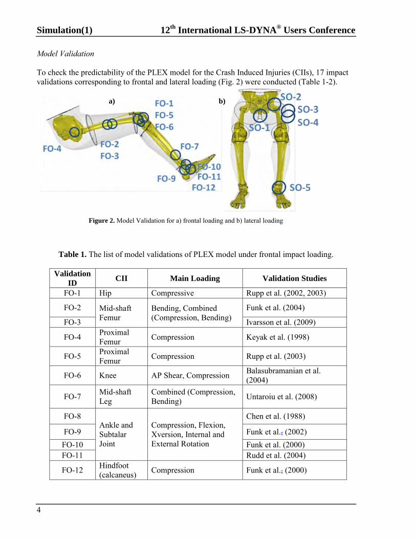
Model Validation To check the predictability of the PLEX model for the Crash Induced Injuries (CIIs), 17 impact validations corresponding to frontal and lateral loading (Fig. 2) were conducted (Table 1-2).

Figure 2. Model Validation for a) frontal loading and b) lateral loading

a) b)

Table 1. The list of model validations of PLEX model under frontal impact loading.

Validation

ID CII Main Loading Validation Studies

FO-1 Hip Compressive Rupp et al. (2002, 2003)

FO-2 Mid-shaft Femur

Bending, Combined (Compression, Bending)

Funk et al. (2004)

FO-3 Ivarsson et al. (2009)

FO-4 Proximal Femur Compression Keyak et al. (1998)

FO-5 Proximal Femur Compression Rupp et al. (2003)

FO-6 Knee AP Shear, Compression Balasubramanian et al. (2004)

FO-7 Mid-shaft Leg

Combined (Compression, Bending) Untaroiu et al. (2008)

FO-8 Ankle and Subtalar Joint

Compression, Flexion, Xversion, Internal and External Rotation

Chen et al. (1988)

FO-9 Funk et al., (2002) FO-10 Funk et al. (2000) FO-11 Rudd et al. (2004)

FO-12 Hindfoot (calcaneus) Compression Funk et al., (2000)

12th


5

The FE models of test set ups were developed and then were connected with the PLEX models to accurately replicate boundary conditions corresponding to PMHS component tests. The input data in the component validations was usually defined as the time histories of impactors recorded in testing. The time histories of impact loading and the injuries predicted by the models were recorded and compared with PMHS test data. Stability Check of the FE Model under Severe Impact Loading Condition

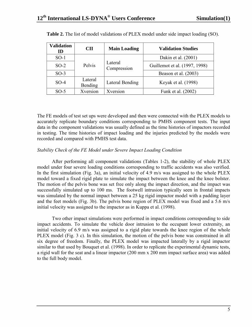
After performing all component validations (Tables 1-2), the stability of whole PLEX model under four severe loading conditions corresponding to traffic accidents was also verified. In the first simulation (Fig. 3a), an initial velocity of 4.9 m/s was assigned to the whole PLEX model toward a fixed rigid plate to simulate the impact between the knee and the knee bolster. The motion of the pelvis bone was set free only along the impact direction, and the impact was successfully simulated up to 100 ms. The footwell intrusion typically seen in frontal impacts was simulated by the normal impact between a 25 kg rigid impactor model with a padding layer and the feet models (Fig. 3b). The pelvis bone region of PLEX model was fixed and a 5.6 m/s initial velocity was assigned to the impactor as in Kuppa et al. (1998).

Two other impact simulations were performed in impact conditions corresponding to side

impact accidents. To simulate the vehicle door intrusion to the occupant lower extremity, an initial velocity of 6.9 m/s was assigned to a rigid plate towards the knee region of the whole PLEX model (Fig. 3 c). In this simulation, the motion of the pelvis bone was constrained in all six degree of freedom. Finally, the PLEX model was impacted laterally by a rigid impactor similar to that used by Bouquet et al. (1998). In order to replicate the experimental dynamic tests, a rigid wall for the seat and a linear impactor (200 mm x 200 mm impact surface area) was added to the full body model.

Table 2. The list of model validations of PLEX model under side impact loading (SO).

Validation

ID CII Main Loading Validation Studies

SO-1 Pelvis Lateral

Compression

Dakin et al. (2001) SO-2 Guillemot et al. (1997, 1998) SO-3 Beason et al. (2003)

SO-4 Lateral Bending Lateral Bending Keyak et al. (1998)

SO-5 Xversion Xversion Funk et al. (2002)

Simulation(1) 12th


6

Results and Discussion

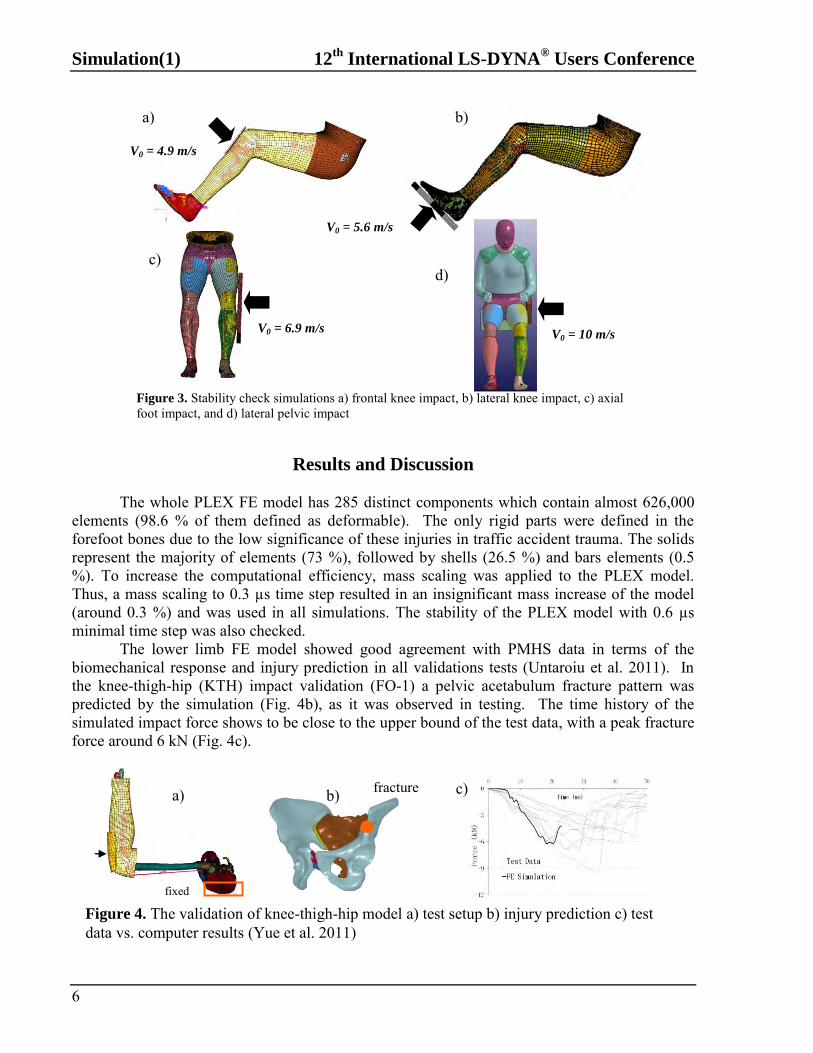
The whole PLEX FE model has 285 distinct components which contain almost 626,000 elements (98.6 % of them defined as deformable). The only rigid parts were defined in the forefoot bones due to the low significance of these injuries in traffic accident trauma. The solids represent the majority of elements (73 %), followed by shells (26.5 %) and bars elements (0.5 %). To increase the computational efficiency, mass scaling was applied to the PLEX model. Thus, a mass scaling to 0.3 µs time step resulted in an insignificant mass increase of the model (around 0.3 %) and was used in all simulations. The stability of the PLEX model with 0.6 µs minimal time step was also checked. The lower limb FE model showed good agreement with PMHS data in terms of the biomechanical response and injury prediction in all validations tests (Untaroiu et al. 2011). In the knee-thigh-hip (KTH) impact validation (FO-1) a pelvic acetabulum fracture pattern was predicted by the simulation (Fig. 4b), as it was observed in testing. The time history of the simulated impact force shows to be close to the upper bound of the test data, with a peak fracture force around 6 kN (Fig. 4c).

Figure 3. Stability check simulations a) frontal knee impact, b) lateral knee impact, c) axial foot impact, and d) lateral pelvic impact

V0 = 4.9 m/s

b) a)

V0 = 6.9 m/s

V0 = 5.6 m/s

d)

V0 = 10 m/s

c)

Figure 4. The validation of knee-thigh-hip model a) test setup b) injury prediction c) test data vs. computer results (Yue et al. 2011)

fixed

fracture a) b) c)

12th


7

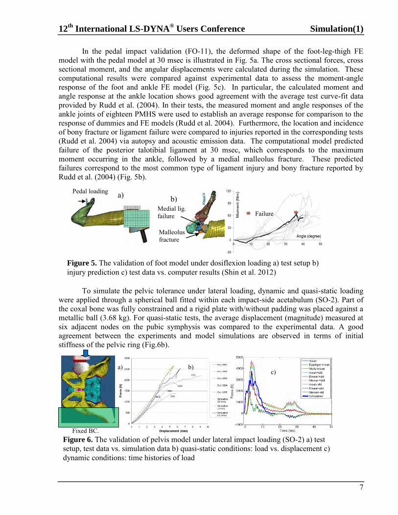
In the pedal impact validation (FO-11), the deformed shape of the foot-leg-thigh FE model with the pedal model at 30 msec is illustrated in Fig. 5a. The cross sectional forces, cross sectional moment, and the angular displacements were calculated during the simulation. These computational results were compared against experimental data to assess the moment-angle response of the foot and ankle FE model (Fig. 5c). In particular, the calculated moment and angle response at the ankle location shows good agreement with the average test curve-fit data provided by Rudd et al. (2004). In their tests, the measured moment and angle responses of the ankle joints of eighteen PMHS were used to establish an average response for comparison to the response of dummies and FE models (Rudd et al. 2004). Furthermore, the location and incidence of bony fracture or ligament failure were compared to injuries reported in the corresponding tests (Rudd et al. 2004) via autopsy and acoustic emission data. The computational model predicted failure of the posterior talotibial ligament at 30 msec, which corresponds to the maximum moment occurring in the ankle, followed by a medial malleolus fracture. These predicted failures correspond to the most common type of ligament injury and bony fracture reported by Rudd et al. (2004) (Fig. 5b).

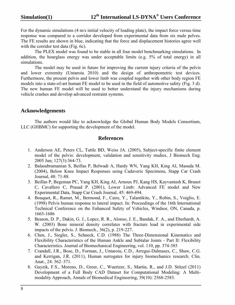
To simulate the pelvic tolerance under lateral loading, dynamic and quasi-static loading were applied through a spherical ball fitted within each impact-side acetabulum (SO-2). Part of the coxal bone was fully constrained and a rigid plate with/without padding was placed against a metallic ball (3.68 kg). For quasi-static tests, the average displacement (magnitude) measured at six adjacent nodes on the pubic symphysis was compared to the experimental data. A good agreement between the experiments and model simulations are observed in terms of initial stiffness of the pelvic ring (Fig.6b).

Figure 5. The validation of foot model under dosiflexion loading a) test setup b) injury prediction c) test data vs. computer results (Shin et al. 2012)

Pedal loading a) b) c)

Malleolus fracture

Medial lig. failure fracture

b) c)

a)

Figure 6. The validation of pelvis model under lateral impact loading (SO-2) a) test setup, test data vs. simulation data b) quasi-static conditions: load vs. displacement c) dynamic conditions: time histories of load

Fixed BC.

Failure

Simulation(1) 12th


8

For the dynamic simulations (4 m/s initial velocity of loading plate), the impact force versus time response was compared to a corridor developed from experimental data from six male pelves. The FE results are shown in blue, indicating that the force and displacement histories agree well with the corridor test data (Fig. 6c). The PLEX model was found to be stable in all four model benchmarking simulations. In addition, the hourglass energy was under acceptable limits (e.g. 5% of total energy) in all simulations. The model may be used in future for improving the current injury criteria of the pelvis and lower extremity (Untaroiu 2010) and the design of anthropometric test devices. Furthermore, the present pelvis and lower limb was coupled together with other body region FE models into a state-of-art human FE model to be used in the field of automotive safety (Fig. 3 d). The new human FE model will be used to better understand the injury mechanisms during vehicle crashes and develop advanced restraint systems. Acknowledgements The authors would like to acknowledge the Global Human Body Models Consortium, LLC (GHBMC) for supporting the development of the model.

References

1. Anderson AE, Peters CL, Tuttle BD, Weiss JA. (2005), Subject-specific finite element

model of the pelvis: development, validation and sensitivity studies, J Biomech Eng. 2005 Jun; 127(3):364-73.

2. Balasubramanian S, Beillas P, Belwadi A, Hardy WN, Yang KH, King AI, Masuda M. (2004), Below Knee Impact Responses using Cadaveric Specimens, Stapp Car Crash Journal, 48: 71-88.

3. Beillas P, Begeman PC, Yang KH, King AI, Arnoux PJ, Kang HS, Kayvantash K, Brunet C, Cavallero C, Prasad P. (2001), Lower Limb: Advanced FE model and New Experimental Data, Stapp Car Crash Journal, 45: 469-494.

4. Bouquet, R., Ramet, M., Bermond, F., Caire, Y., Talantikite, Y., Robin, S., Voiglio, E. (1998) Pelvis human response to lateral impact. In: Proceedings of the 16th International Technical Conference on the Enhanced Safety of Vehicles, Windsor, ON, Canada, p. 1665-1686

5. Beason, D. P., Dakin, G. J., Lopez, R. R., Alonso, J. E., Bandak, F. A., and Eberhardt, A. W. (2003) Bone mineral density correlates with fracture load in experimental side impacts of the pelvis. J. Biomech., 36(2), p. 219-227.

6. Chen, J., Siegler, S., Schneck, C.D. (1988) The Three-Dimensional Kinematics and Flexibility Characteristics of the Human Ankle and Subtalar Joints - Part II: Flexibility Characteristics. Journal of Biomechanical Engineering, vol. 110, pp. 374-385

7. Crandall, J.R., Bose, D., Forman, J., Untaroiu, C.D., Arregui-Dalmases, C., Shaw, C.G. and Kerrigan, J.R. (2011), Human surrogates for injury biomechanics research. Clin. Anat., 24: 362–371.

8. Gayzik, F.S., Moreno, D., Greer, C., Wuertzer, S., Martin, R., and J.D. Stitzel (2011) Development of a Full Body CAD Dataset for Computational Modeling: A Multi-modality Approach, Annals of Biomedical Engineering, 39(10): 2568-2583.

12th


9

9. Gordon, C.C., Churchill, T., Clauser, C.E., Bradtmiller, B., McConville, J.T., Tebbetts , I., Walker , R.A., 1989. 1988 anthropometric survey of US army personnel: methods and summary statistics. (NATICK/TR-89/044). US Army Natick Research, Development, and Engineering Center, Natick, MA.

10. Hewitt J, Guilak F, Glisson R, and TP Vail (2001), Regional Material Properties of the Human Hip Joint Capsule Ligaments, Journal of Orthopaedic Research, 19 (359-64).

11. Haug, E. (2001), H-Model Overview Description, Proceedings of the Twenty-Ninth International Workshop on Human Subjects for Injury Biomechanics Research.

12. Funk, J. R., Kerrigan, J. R. and Crandall, J. R., "Dynamic Bending Tolerance and Elastic-Plastic Material Properties of the Human Femur", 48th Annual Proceedings of AAAM, 2004.

13. Funk, J., Tourret, L., George, S., Crandall, J.R. (2000) The Role of Axial Loading in Malleolar Fractures. Paper 2000-01-0155, Society of Automotive Engineers.

14. Funk, J., Srinivasan, S., Crandall, J.R., Khaewpong, N., Eppinger, R., Jaffredo, A., Potier, P., Petit, P. (2002) The Effects of Axial Preload and Dorsiflexion on the Tolerance of the Ankle/Subtalar Joint to Dynamic Inversion and Eversion. Proceedings of the 46th Stapp Car Crash Conference, SAE paper 2002-22-0013.

15. Guillemot, H., Got, C., Besault, B., Lavaste, F., Robin, S., Le Coz, J. Y., and Lassau, J. (1998) Pelvic behavior in side collisions: static and dynamic tests on isolated pelvic bones. In: Proceedings of the 16th ESV Conference. Windsor, ON, Canada, p. 14412–14424.

16. Ivarsson BJ, Genovese D, Crandall JR, Bolton J, Untaroiu C, Bose D. (2009) The tolerance of the femoral shaft in combined axial compression and bending loading. Stapp Car Crash Journal; 53:251-290.

17. Keyak, J. H., Rossi, S. A., Jones, K. A. et al., “Prediction of femoral fracture load using automated finite element modeling”, Journal of Biomechanics, 31:125-133, 1998

18. Kim YS, Choi HH, Cho YN, Park YJ, Lee JB, Yang KH, and AI King (2005), Numerical Investigations of Interactions between the Knee-Thigh-Hip Complex with Vehicle Interior Structures, Stapp Car Crash Journal, 49:85-115.

19. Kim, Y.H., Kim, J.E., Eberhardt, A.W., “A New Cortical Thickness Mapping Method with Application to an In-Vivo Finite Element Model, in review, Computer Methods in Biomechanics and Biomedical Engineering.

20. Kuppa, (1998) Axial Impact Characteristics of Dummy and Cadaver Lower Limbs, 16th ESV, Vol 2, pp 1608-1617.

21. Morgan, R.M., Eppinger, R., Marcus, J., and H. Nichols (1990) Human cadaver and hybrid III responses to axial impacts of the femur. Proceedings of the International IRCOBI on Biomechanics Impacts.

22. Robbins, D. H., Schneider, L. W. and Haffner, M., Seated Posture of Vehicle Occupants, Stapp Car Crash Conference Proceedings, # 831617, 1983.

23. Rudd, R., Crandall, J., Millington, S., Hurwitz, S. (2004) Injury Tolerance and Response of the Ankle Joint in Dynamic Dorsiflexion. Stapp Car Crash Journal, 48:1-26.

24. Silvestri, C. and M.H. Ray (2009) Development of a Finite Element Model of the Knee-thigh-hip of a 50 percentile male including ligaments and muscles, International Journal of Crashworthiness, 14 (2).

25. Shin, J., Yue, N., Untaroiu C.D. (2012) A Finite Element Model of the Foot and Ankle for Automotive Impact Applications, Annals of Biomedical Engineering, (under review).

Simulation(1) 12th


10

26. Takahashi, Y., Kikuchi, Y., Konosu, A. and, H. Ishikawa (2000), Development and Validation of the Finite Element Model for the Human Lower Limb of Pedestrians, Stapp Car Crash Journal, 2000-01-SC22.

27. Untaroiu, C.D. (2005), Development and Validation of a Finite Element Model of Human Lower Limb, Ph.D dissertation, Department of Mechanical and Aerospace Engineering, University of Virginia, Charlottesville.

28. Untaroiu CD, Ivarsson BJ, Genovese D, Bose D, Crandall JR. Biomechanical injury response of leg subjected to dynamic combined axial and bending loading. Biomedical Sciences Instrumentation 2008; 44:141–146.

29. Untaroiu, C.D. (2010) “A numerical investigation of mid-femoral injury tolerance in axial compression and bending loading”, International Journal of Crashworthiness, (Impact factor 0.607, ISI citations: 2), 15(1):83-92.

30. Untaroiu, CD et al. (2011) The Finite Element Model of the GHBMC Pelvis and Lower Extremities (LS-Dyna Version), User Manual.

31. Wheeler L, Manning P, Owen C et al (2000). Biofidelity of dummy legs for use in legislative crash testing. International Vehicle Safety 2000 Conference Transactions, London, England, 2000, pp 183-200.

32. Yamada, H. (1970), Strength of Biological Materials, The Williams & Wilkins Company, Baltimore.

33. Yue N., Shin J., Untaroiu C.D., (2011) A Numerical Investigation of Biomechanical and Injury Response of Occupant Lower Extremity during Automotive Crashes, NHTSA Workshop.

12th


1

Development of Tied Overlapping Shell Technique to

Simulate the Path of Crack Propagation in Polymer Parts

Shigeki Kojima, Katsuya Ishibashi TOYOTA TECHNICAL DEVELOPMENT CORPORATION

Tsuyoshi Yasuki, Hideaki Arimoto

Toyota Motor Corporation

Abstract This paper describes a new finite element modeling technique to simulate the path of crack propagation in polymer parts. In this new technique "tied overlapping shell technique", base and overlapping elements make up the finite element model surface. The overlapping elements are rotated 45 degrees with respect to the base elements and are connected by tied contact. Tied overlapping shell technique decreased mesh pattern dependency of FE crack propagation. Tied overlapping shell technique was applied to a polymer door trim model, and impactor crash FE analysis was performed. The result of the FE crack propagation path with the new technique correlated with the experimental result.

1. Introduction

Finite element (hereinafter referred to as "FE") analysis has been increasingly used in helping develop the crash performance of vehicles. In a crash FE analysis including occupant safety, it is useful to accurately predict not only the airbag deployment but also the deformed shape of polymer interior parts. Since polymer interior part deformation may include crack propagation in collisions, it is also useful to predict the crack propagation of polymer interior parts. Many FE analysis techniques have been developed for simulations of crack propagation. Tabiei et al.(2002) have developed an FE analysis method with the automated fracture procedure. To predict the path of crack propagation precisely, elements need to be aligned with the crack propagation direction at the crack tip. The automated fracture procedure aligns elements with the crack propagation direction in a remesh process, and predicts the path of crack propagation by repeated remesh processes. It is not easy to apply this method to an FE crash analysis with a large full vehicle model. Instead, a more suitable method of element deletion has been used to simulate crack propagation in explicit codes such as LS-DYNA®. However, in this method, it is difficult to simulate actual crack propagation because the mesh pattern may not be aligned with the crack propagation direction (hereinafter referred to as "mesh pattern dependency of crack propagation"). Xue et al. (2006) have reported improvement of the element deletion criteria for crack propagation, but no method for the decrease of mesh pattern dependency in predicting crack propagation has been reported. This paper describes the development of a new modeling method to decrease the mesh pattern dependency of crack propagation and the verification of the crack propagation path between a polymer door trim impact experiment and FE analysis with the new modeling method.

Simulation(1) 12th


2

2. Methods

2.1 Tied Overlapping Shell Technique

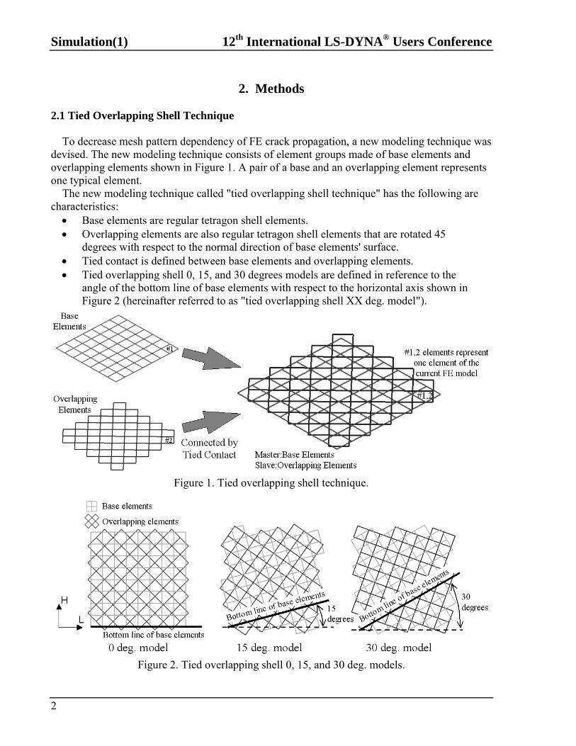
To decrease mesh pattern dependency of FE crack propagation, a new modeling technique was devised. The new modeling technique consists of element groups made of base elements and overlapping elements shown in Figure 1. A pair of a base and an overlapping element represents one typical element. The new modeling technique called "tied overlapping shell technique" has the following are characteristics: Base elements are regular tetragon shell elements. Overlapping elements are also regular tetragon shell elements that are rotated 45

degrees with respect to the normal direction of base elements' surface. Tied contact is defined between base elements and overlapping elements. Tied overlapping shell 0, 15, and 30 degrees models are defined in reference to the

angle of the bottom line of base elements with respect to the horizontal axis shown in Figure 2 (hereinafter referred to as "tied overlapping shell XX deg. model").

Figure 1. Tied overlapping shell technique.

Figure 2. Tied overlapping shell 0, 15, and 30 deg. models.

12th


3

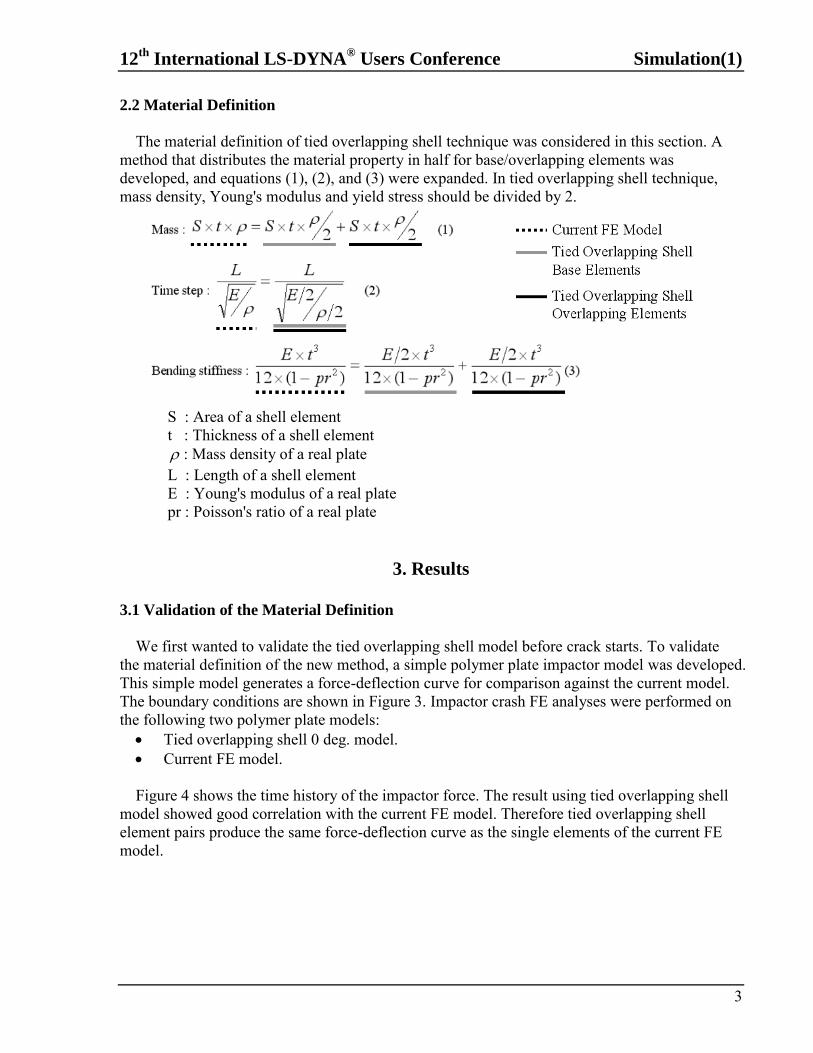
2.2 Material Definition

The material definition of tied overlapping shell technique was considered in this section. A method that distributes the material property in half for base/overlapping elements was developed, and equations (1), (2), and (3) were expanded. In tied overlapping shell technique, mass density, Young's modulus and yield stress should be divided by 2. S : Area of a shell element t : Thickness of a shell element : Mass density of a real plate L : Length of a shell element E : Young's modulus of a real plate pr : Poisson's ratio of a real plate

3. Results

3.1 Validation of the Material Definition

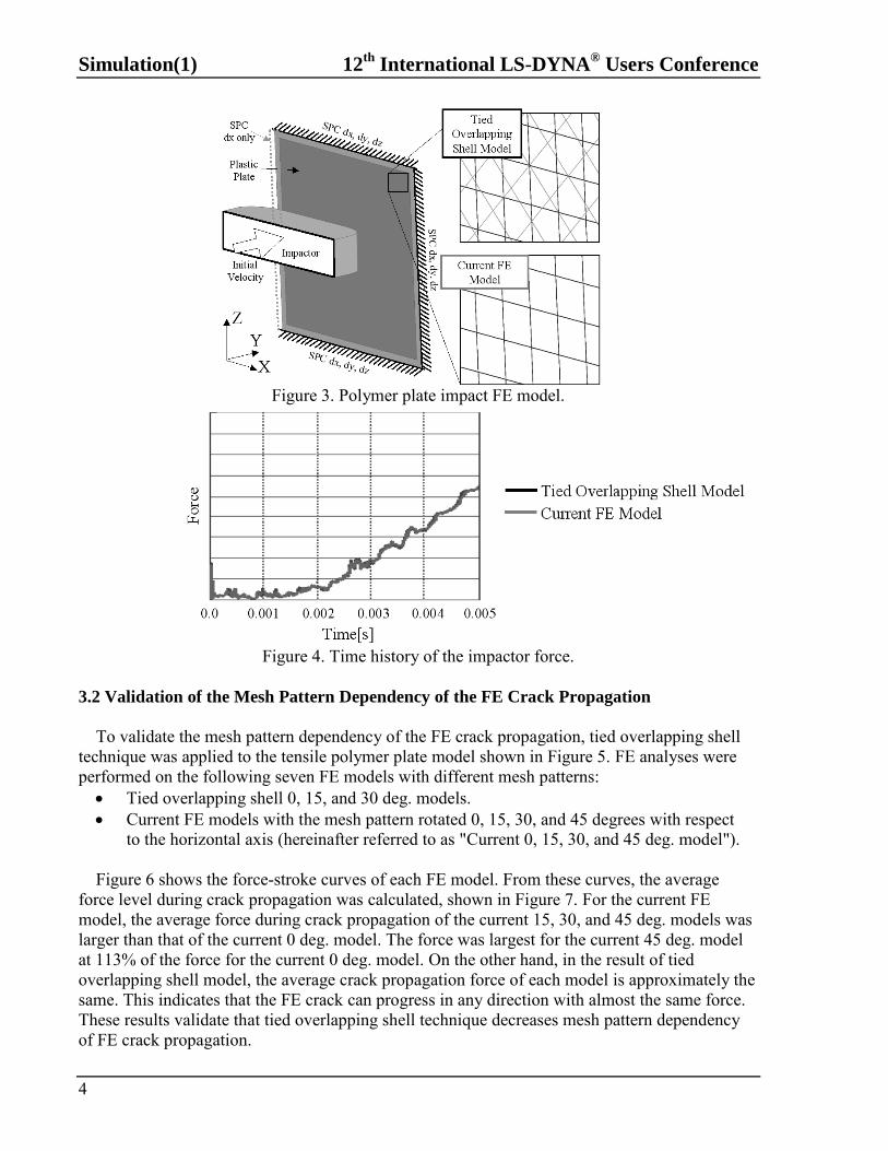
We first wanted to validate the tied overlapping shell model before crack starts. To validate the material definition of the new method, a simple polymer plate impactor model was developed. This simple model generates a force-deflection curve for comparison against the current model. The boundary conditions are shown in Figure 3. Impactor crash FE analyses were performed on the following two polymer plate models: Tied overlapping shell 0 deg. model. Current FE model.

Figure 4 shows the time history of the impactor force. The result using tied overlapping shell model showed good correlation with the current FE model. Therefore tied overlapping shell element pairs produce the same force-deflection curve as the single elements of the current FE model.

Simulation(1) 12th


4

Figure 3. Polymer plate impact FE model.

Figure 4. Time history of the impactor force. 3.2 Validation of the Mesh Pattern Dependency of the FE Crack Propagation

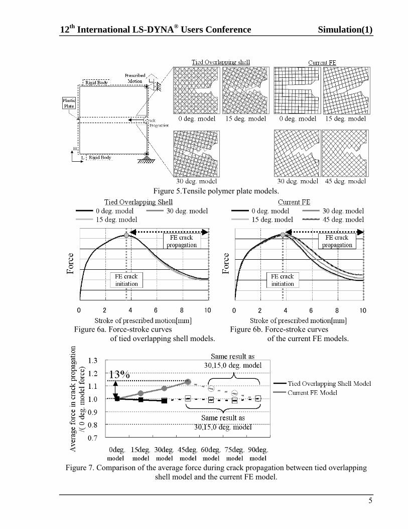
To validate the mesh pattern dependency of the FE crack propagation, tied overlapping shell technique was applied to the tensile polymer plate model shown in Figure 5. FE analyses were performed on the following seven FE models with different mesh patterns: Tied overlapping shell 0, 15, and 30 deg. models. Current FE models with the mesh pattern rotated 0, 15, 30, and 45 degrees with respect

to the horizontal axis (hereinafter referred to as "Current 0, 15, 30, and 45 deg. model"). Figure 6 shows the force-stroke curves of each FE model. From these curves, the average force level during crack propagation was calculated, shown in Figure 7. For the current FE model, the average force during crack propagation of the current 15, 30, and 45 deg. models was larger than that of the current 0 deg. model. The force was largest for the current 45 deg. model at 113% of the force for the current 0 deg. model. On the other hand, in the result of tied overlapping shell model, the average crack propagation force of each model is approximately the same. This indicates that the FE crack can progress in any direction with almost the same force. These results validate that tied overlapping shell technique decreases mesh pattern dependency of FE crack propagation.

12th


5

Figure 5.Tensile polymer plate models. Figure 6a. Force-stroke curves Figure 6b. Force-stroke curves of tied overlapping shell models. of the current FE models.

Figure 7. Comparison of the average force during crack propagation between tied overlapping shell model and the current FE model.

Simulation(1) 12th


6

3.3 Verification of the FE Analysis using Tied Overlapping Shell Technique

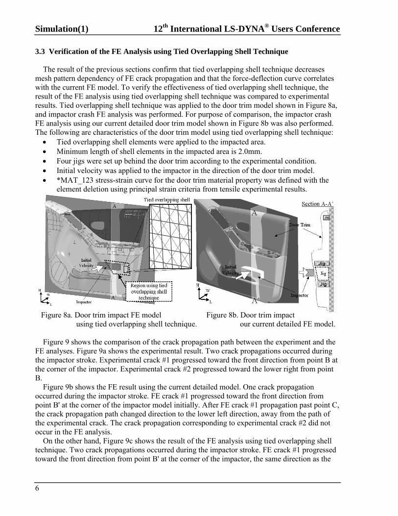
The result of the previous sections confirm that tied overlapping shell technique decreases mesh pattern dependency of FE crack propagation and that the force-deflection curve correlates with the current FE model. To verify the effectiveness of tied overlapping shell technique, the result of the FE analysis using tied overlapping shell technique was compared to experimental results. Tied overlapping shell technique was applied to the door trim model shown in Figure 8a, and impactor crash FE analysis was performed. For purpose of comparison, the impactor crash FE analysis using our current detailed door trim model shown in Figure 8b was also performed. The following are characteristics of the door trim model using tied overlapping shell technique: Tied overlapping shell elements were applied to the impacted area. Minimum length of shell elements in the impacted area is 2.0mm. Four jigs were set up behind the door trim according to the experimental condition. Initial velocity was applied to the impactor in the direction of the door trim model. *MAT_123 stress-strain curve for the door trim material property was defined with the

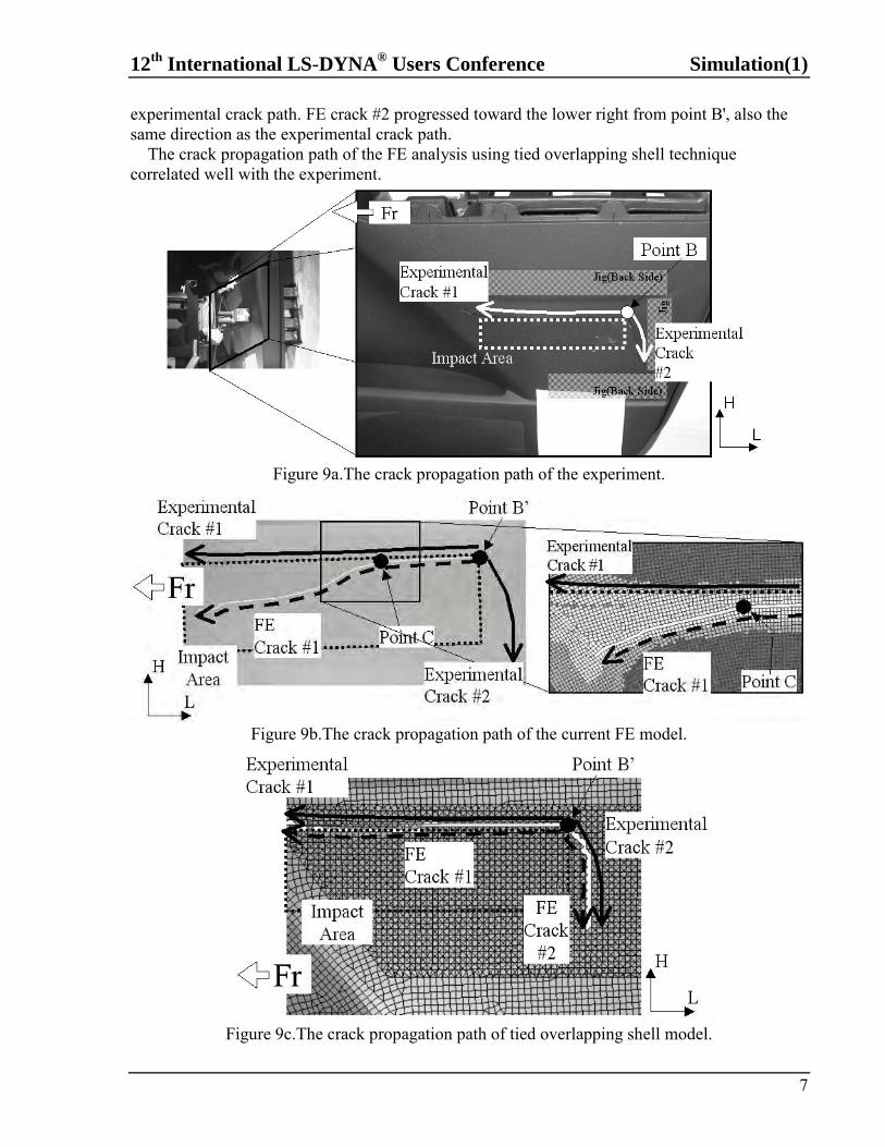
element deletion using principal strain criteria from tensile experimental results. Figure 8a. Door trim impact FE model Figure 8b. Door trim impact using tied overlapping shell technique. our current detailed FE model. Figure 9 shows the comparison of the crack propagation path between the experiment and the FE analyses. Figure 9a shows the experimental result. Two crack propagations occurred during the impactor stroke. Experimental crack #1 progressed toward the front direction from point B at the corner of the impactor. Experimental crack #2 progressed toward the lower right from point B. Figure 9b shows the FE result using the current detailed model. One crack propagation occurred during the impactor stroke. FE crack #1 progressed toward the front direction from point B' at the corner of the impactor model initially. After FE crack #1 propagation past point C, the crack propagation path changed direction to the lower left direction, away from the path of the experimental crack. The crack propagation corresponding to experimental crack #2 did not occur in the FE analysis. On the other hand, Figure 9c shows the result of the FE analysis using tied overlapping shell technique. Two crack propagations occurred during the impactor stroke. FE crack #1 progressed toward the front direction from point B' at the corner of the impactor, the same direction as the

12th


7

experimental crack path. FE crack #2 progressed toward the lower right from point B', also the same direction as the experimental crack path. The crack propagation path of the FE analysis using tied overlapping shell technique correlated well with the experiment.

Figure 9a.The crack propagation path of the experiment.

Figure 9b.The crack propagation path of the current FE model.

Figure 9c.The crack propagation path of tied overlapping shell model.

Simulation(1) 12th


8

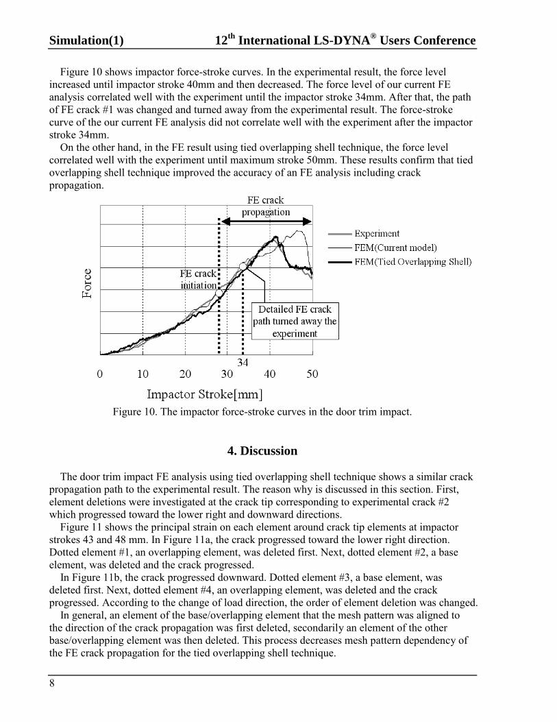
Figure 10 shows impactor force-stroke curves. In the experimental result, the force level increased until impactor stroke 40mm and then decreased. The force level of our current FE analysis correlated well with the experiment until the impactor stroke 34mm. After that, the path of FE crack #1 was changed and turned away from the experimental result. The force-stroke curve of the our current FE analysis did not correlate well with the experiment after the impactor stroke 34mm. On the other hand, in the FE result using tied overlapping shell technique, the force level correlated well with the experiment until maximum stroke 50mm. These results confirm that tied overlapping shell technique improved the accuracy of an FE analysis including crack propagation.

Figure 10. The impactor force-stroke curves in the door trim impact.

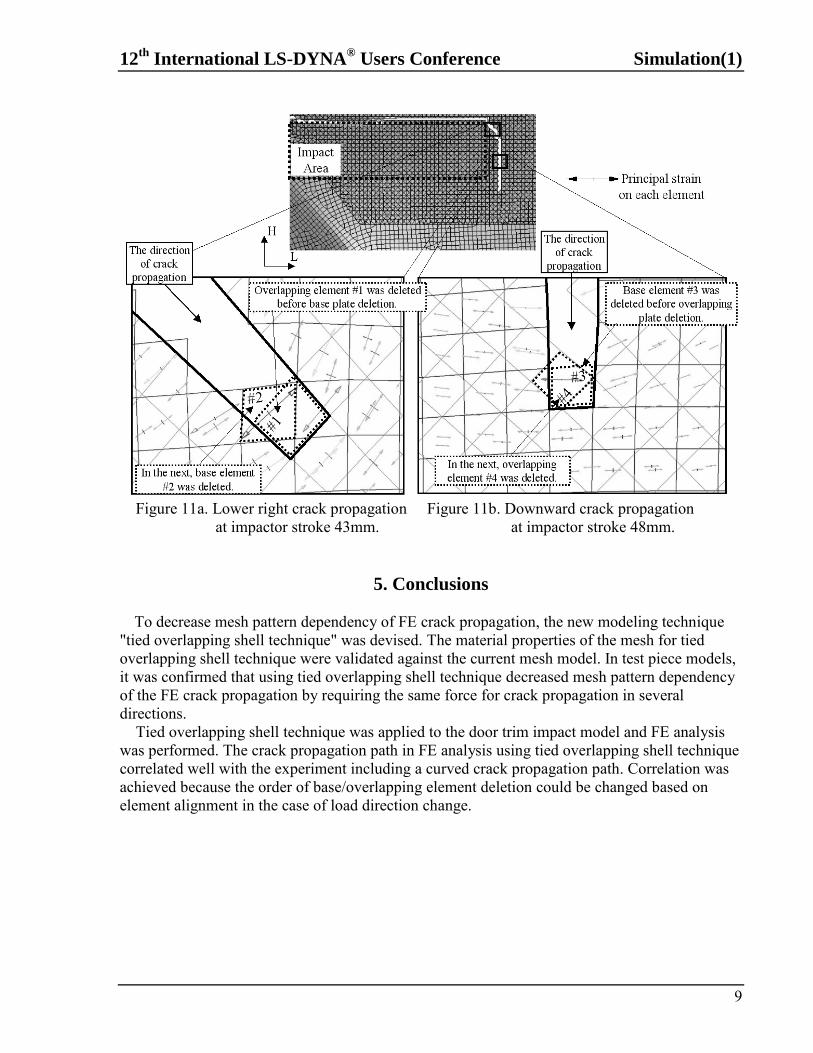
4. Discussion The door trim impact FE analysis using tied overlapping shell technique shows a similar crack propagation path to the experimental result. The reason why is discussed in this section. First, element deletions were investigated at the crack tip corresponding to experimental crack #2 which progressed toward the lower right and downward directions. Figure 11 shows the principal strain on each element around crack tip elements at impactor strokes 43 and 48 mm. In Figure 11a, the crack progressed toward the lower right direction. Dotted element #1, an overlapping element, was deleted first. Next, dotted element #2, a base element, was deleted and the crack progressed. In Figure 11b, the crack progressed downward. Dotted element #3, a base element, was deleted first. Next, dotted element #4, an overlapping element, was deleted and the crack progressed. According to the change of load direction, the order of element deletion was changed. In general, an element of the base/overlapping element that the mesh pattern was aligned to the direction of the crack propagation was first deleted, secondarily an element of the other base/overlapping element was then deleted. This process decreases mesh pattern dependency of the FE crack propagation for the tied overlapping shell technique.

12th


9

Figure 11a. Lower right crack propagation Figure 11b. Downward crack propagation at impactor stroke 43mm. at impactor stroke 48mm.

5. Conclusions To decrease mesh pattern dependency of FE crack propagation, the new modeling technique "tied overlapping shell technique" was devised. The material properties of the mesh for tied overlapping shell technique were validated against the current mesh model. In test piece models, it was confirmed that using tied overlapping shell technique decreased mesh pattern dependency of the FE crack propagation by requiring the same force for crack propagation in several directions. Tied overlapping shell technique was applied to the door trim impact model and FE analysis was performed. The crack propagation path in FE analysis using tied overlapping shell technique correlated well with the experiment including a curved crack propagation path. Correlation was achieved because the order of base/overlapping element deletion could be changed based on element alignment in the case of load direction change.

Simulation(1) 12th


10

References

LS-DYNA user manual V971, Livermore Software Technology Corporation. Tabiei, A., Wu, J.(2002), Development of The DYNA3D Simulation Code with Automated Fracture Procedure for

Brick Elements, 7th International LS-DYNA Users Conference, Dearborn. Xue, L., Wierzbicki, T.(2006), Verification of a New Fracture Criterion Using LS-DYNA, 9th International LS-

DYNA Users Conference, Dearborn.

12th


1

Techniques for Modeling Torque Transfer between

Concentric Cylindrical Components

Richard Tejeda InForm Product Development, Inc.

Abstract Finite elements that use a piecewise linear approximation of geometry are perfectly adequate for modeling cylindrical components such as shafts and hubs in many applications. However, linear elements present a challenge to the assessment of contact interfaces between curved surfaces, namely that faceted surfaces have peaks and valleys that can interlock with each other. A good example is when torque is transferred between a shaft and a hub via a key, collar, pin, or some other means. In this case, it can be difficult or impossible to control how the applied torque is shared between the interlocking mesh and the intended torque transfer device. If the goal of the analysis is to determine the strength of the actual torque transfer features (e.g., a keyway or spline), then it is critical to apply the correct load to them by eliminating or at least minimizing mesh interlocking. This paper discusses various strategies for circumventing the mesh interlocking problem.

Introduction When finite elements that use a piecewise linear approximation of geometry are applied to a surface with curvature, the result is a faceted surface. Deviations from the true surface decrease when smaller elements are used, but the high and low spots can never be eliminated from the mesh. Faceted surfaces are often of little consequence, but they can make it difficult to accurately assess the contact interactions between a shaft and the bore of a mating component such as a gear, cam, or pulley. The problem is that the inevitable peaks and valleys on the meshed surfaces of the two components will interlock with each other and transfer loads in a non-physical manner. Even worse, the degree of interlocking can vary between different meshes, even if the nominal element size is the same. There are a number of ways to deal with the mesh interlocking problem, but none of them work in every situation. This paper will describe some ways to approach this issue in LS-DYNA® MPP 971 R5.1.1 for the case of an 8-inch diameter steel hub mounted on a 4-inch diameter steel shaft. Despite the very specific nature of this example, the techniques described in this paper are applicable to many other instances of curved surface contact.

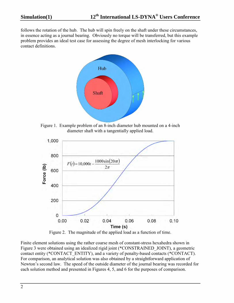
Journal Bearing Test Case Before considering torque transfer between components, it is instructive to examine a frictionless line-on-line fit between the shaft and hub shown in Figure 1. In this example, the shaft is fixed in space and the force described in Figures 1 and 2 is applied to the hub. A smooth force profile was used in order to minimize artificial dynamic effects. The direction and location of the force

Simulation(1) 12th


2

follows the rotation of the hub. The hub will spin freely on the shaft under these circumstances, in essence acting as a journal bearing. Obviously no torque will be transferred, but this example problem provides an ideal test case for assessing the degree of mesh interlocking for various contact definitions.

Figure 1. Example problem of an 8-inch diameter hub mounted on a 4-inch

diameter shaft with a tangentially applied load.

Figure 2. The magnitude of the applied load as a function of time.

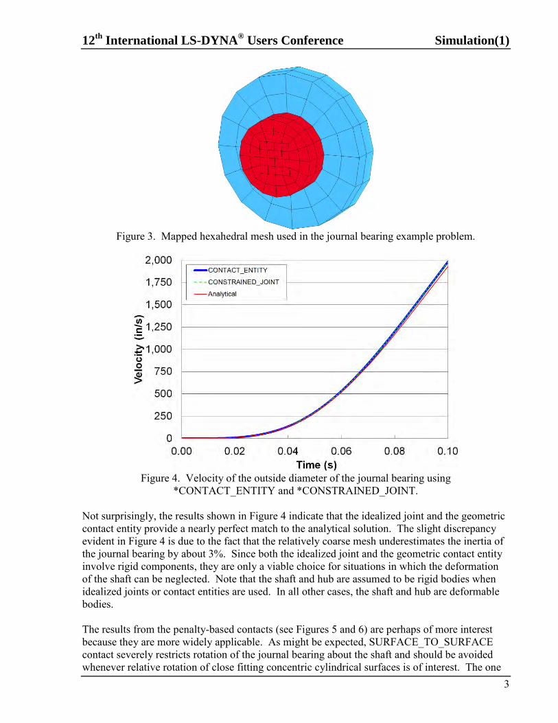
Finite element solutions using the rather coarse mesh of constant-stress hexahedra shown in Figure 3 were obtained using an idealized rigid joint (*CONSTRAINED_JOINT), a geometric contact entity (*CONTACT_ENTITY), and a variety of penalty-based contacts (*CONTACT). For comparison, an analytical solution was also obtained by a straightforward application of Newton’s second law. The speed of the outside diameter of the journal bearing was recorded for each solution method and presented in Figures 4, 5, and 6 for the purposes of comparison.

12th


3

Figure 3. Mapped hexahedral mesh used in the journal bearing example problem.

Figure 4. Velocity of the outside diameter of the journal bearing using

*CONTACT_ENTITY and *CONSTRAINED_JOINT. Not surprisingly, the results shown in Figure 4 indicate that the idealized joint and the geometric contact entity provide a nearly perfect match to the analytical solution. The slight discrepancy evident in Figure 4 is due to the fact that the relatively coarse mesh underestimates the inertia of the journal bearing by about 3%. Since both the idealized joint and the geometric contact entity involve rigid components, they are only a viable choice for situations in which the deformation of the shaft can be neglected. Note that the shaft and hub are assumed to be rigid bodies when idealized joints or contact entities are used. In all other cases, the shaft and hub are deformable bodies. The results from the penalty-based contacts (see Figures 5 and 6) are perhaps of more interest because they are more widely applicable. As might be expected, SURFACE_TO_SURFACE contact severely restricts rotation of the journal bearing about the shaft and should be avoided whenever relative rotation of close fitting concentric cylindrical surfaces is of interest. The one

Simulation(1) 12th


4

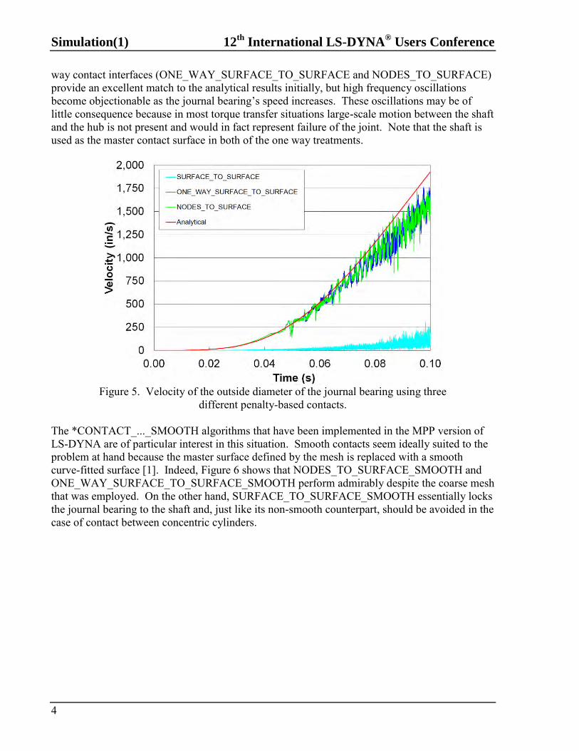
way contact interfaces (ONE_WAY_SURFACE_TO_SURFACE and NODES_TO_SURFACE) provide an excellent match to the analytical results initially, but high frequency oscillations become objectionable as the journal bearing’s speed increases. These oscillations may be of little consequence because in most torque transfer situations large-scale motion between the shaft and the hub is not present and would in fact represent failure of the joint. Note that the shaft is used as the master contact surface in both of the one way treatments.

Figure 5. Velocity of the outside diameter of the journal bearing using three

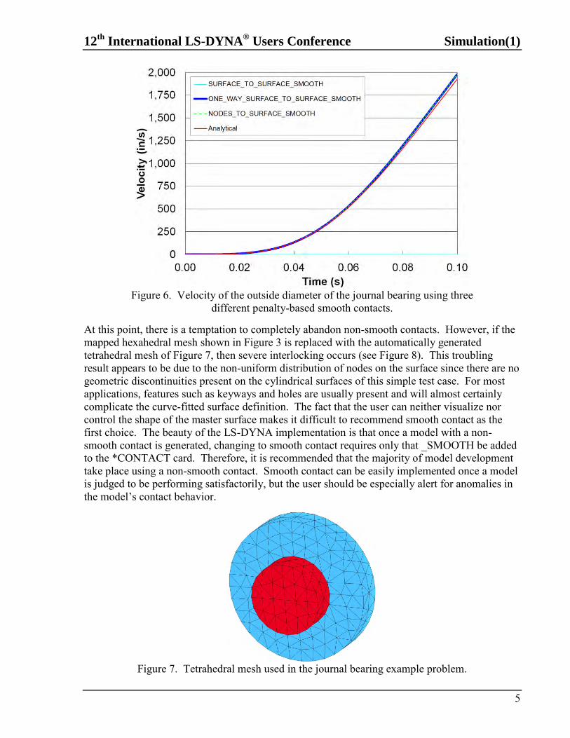
different penalty-based contacts. The *CONTACT_..._SMOOTH algorithms that have been implemented in the MPP version of LS-DYNA are of particular interest in this situation. Smooth contacts seem ideally suited to the problem at hand because the master surface defined by the mesh is replaced with a smooth curve-fitted surface [1]. Indeed, Figure 6 shows that NODES_TO_SURFACE_SMOOTH and ONE_WAY_SURFACE_TO_SURFACE_SMOOTH perform admirably despite the coarse mesh that was employed. On the other hand, SURFACE_TO_SURFACE_SMOOTH essentially locks the journal bearing to the shaft and, just like its non-smooth counterpart, should be avoided in the case of contact between concentric cylinders.

12th


5

Figure 6. Velocity of the outside diameter of the journal bearing using three

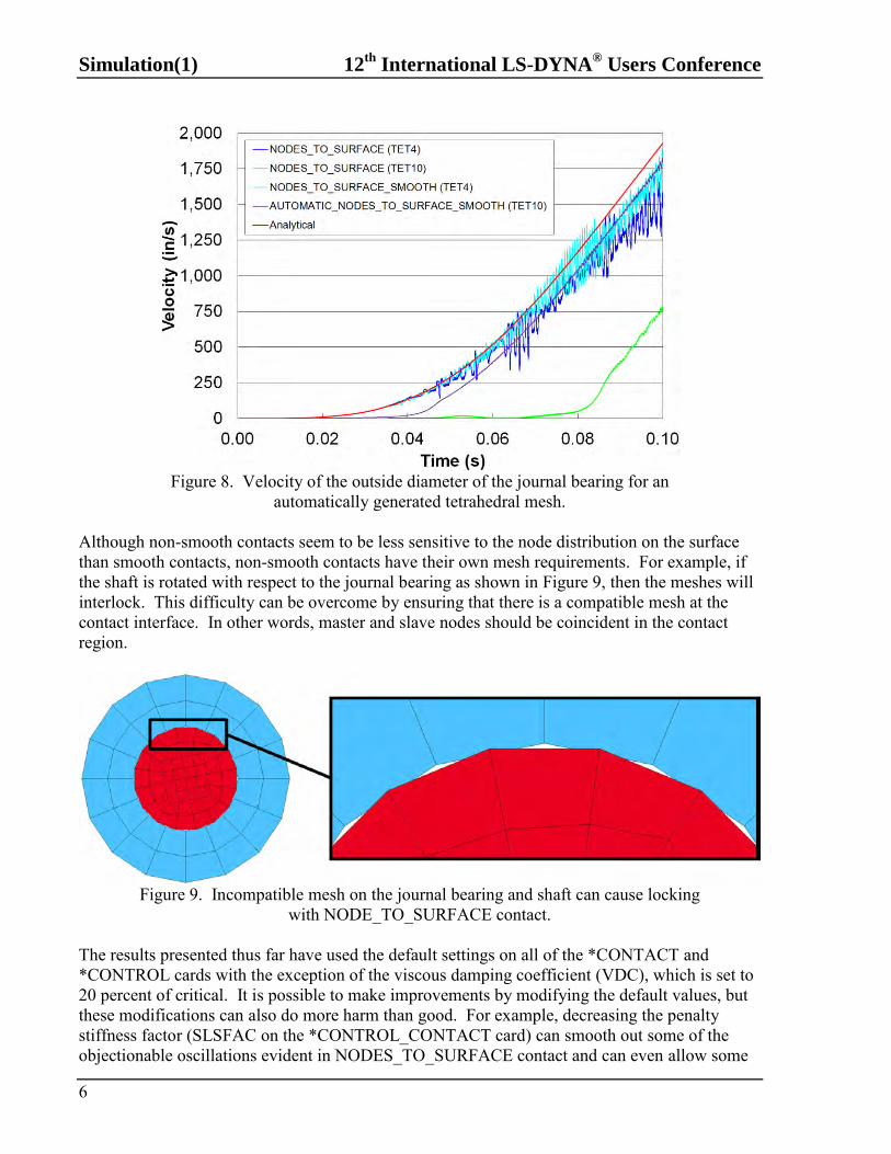
different penalty-based smooth contacts. At this point, there is a temptation to completely abandon non-smooth contacts. However, if the mapped hexahedral mesh shown in Figure 3 is replaced with the automatically generated tetrahedral mesh of Figure 7, then severe interlocking occurs (see Figure 8). This troubling result appears to be due to the non-uniform distribution of nodes on the surface since there are no geometric discontinuities present on the cylindrical surfaces of this simple test case. For most applications, features such as keyways and holes are usually present and will almost certainly complicate the curve-fitted surface definition. The fact that the user can neither visualize nor control the shape of the master surface makes it difficult to recommend smooth contact as the first choice. The beauty of the LS-DYNA implementation is that once a model with a non-smooth contact is generated, changing to smooth contact requires only that _SMOOTH be added to the *CONTACT card. Therefore, it is recommended that the majority of model development take place using a non-smooth contact. Smooth contact can be easily implemented once a model is judged to be performing satisfactorily, but the user should be especially alert for anomalies in the model’s contact behavior.

Figure 7. Tetrahedral mesh used in the journal bearing example problem.

Simulation(1) 12th


6

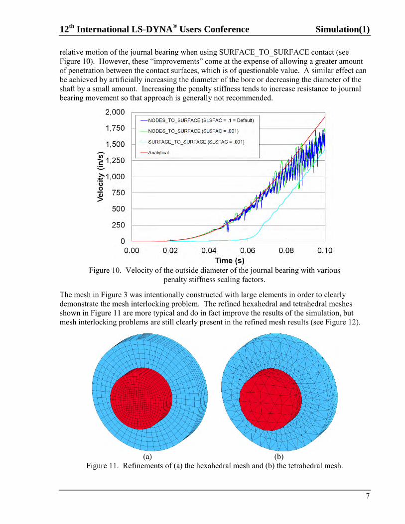
Figure 8. Velocity of the outside diameter of the journal bearing for an

automatically generated tetrahedral mesh. Although non-smooth contacts seem to be less sensitive to the node distribution on the surface than smooth contacts, non-smooth contacts have their own mesh requirements. For example, if the shaft is rotated with respect to the journal bearing as shown in Figure 9, then the meshes will interlock. This difficulty can be overcome by ensuring that there is a compatible mesh at the contact interface. In other words, master and slave nodes should be coincident in the contact region.

Figure 9. Incompatible mesh on the journal bearing and shaft can cause locking

with NODE_TO_SURFACE contact. The results presented thus far have used the default settings on all of the *CONTACT and *CONTROL cards with the exception of the viscous damping coefficient (VDC), which is set to 20 percent of critical. It is possible to make improvements by modifying the default values, but these modifications can also do more harm than good. For example, decreasing the penalty stiffness factor (SLSFAC on the *CONTROL_CONTACT card) can smooth out some of the objectionable oscillations evident in NODES_TO_SURFACE contact and can even allow some

12th


7

relative motion of the journal bearing when using SURFACE_TO_SURFACE contact (see Figure 10). However, these “improvements” come at the expense of allowing a greater amount of penetration between the contact surfaces, which is of questionable value. A similar effect can be achieved by artificially increasing the diameter of the bore or decreasing the diameter of the shaft by a small amount. Increasing the penalty stiffness tends to increase resistance to journal bearing movement so that approach is generally not recommended.

Figure 10. Velocity of the outside diameter of the journal bearing with various

penalty stiffness scaling factors. The mesh in Figure 3 was intentionally constructed with large elements in order to clearly demonstrate the mesh interlocking problem. The refined hexahedral and tetrahedral meshes shown in Figure 11 are more typical and do in fact improve the results of the simulation, but mesh interlocking problems are still clearly present in the refined mesh results (see Figure 12).

(a) (b)

Figure 11. Refinements of (a) the hexahedral mesh and (b) the tetrahedral mesh.

Simulation(1) 12th


8

Figure 12. Velocity of the outside diameter of the journal bearing using various

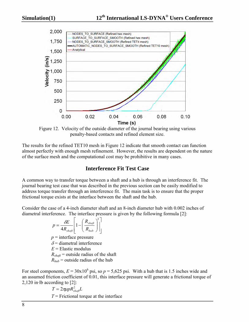
penalty-based contacts and refined element size. The results for the refined TET10 mesh in Figure 12 indicate that smooth contact can function almost perfectly with enough mesh refinement. However, the results are dependent on the nature of the surface mesh and the computational cost may be prohibitive in many cases.

Interference Fit Test Case A common way to transfer torque between a shaft and a hub is through an interference fit. The journal bearing test case that was described in the previous section can be easily modified to address torque transfer through an interference fit. The main task is to ensure that the proper frictional torque exists at the interface between the shaft and the hub. Consider the case of a 4-inch diameter shaft and an 8-inch diameter hub with 0.002 inches of diametral interference. The interface pressure is given by the following formula [2]:

2

14 hub

shaft

shaft RR

REp

p = interface pressure = diametral interference E = Elastic modulus Rshaft = outside radius of the shaft Rhub = outside radius of the hub

For steel components, E = 30x106 psi, so p = 5,625 psi. With a hub that is 1.5 inches wide and an assumed friction coefficient of 0.01, this interface pressure will generate a frictional torque of 2,120 in∙lb according to [2]:

LpRT shaft22

T = Frictional torque at the interface

12th


9

= Coefficient of friction L = Length of the shaft/hub interface

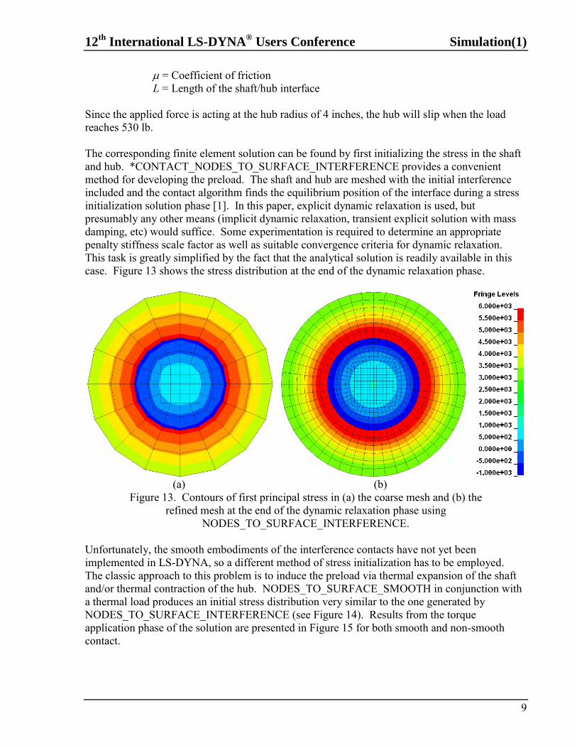
Since the applied force is acting at the hub radius of 4 inches, the hub will slip when the load reaches 530 lb. The corresponding finite element solution can be found by first initializing the stress in the shaft and hub. *CONTACT_NODES_TO_SURFACE_INTERFERENCE provides a convenient method for developing the preload. The shaft and hub are meshed with the initial interference included and the contact algorithm finds the equilibrium position of the interface during a stress initialization solution phase [1]. In this paper, explicit dynamic relaxation is used, but presumably any other means (implicit dynamic relaxation, transient explicit solution with mass damping, etc) would suffice. Some experimentation is required to determine an appropriate penalty stiffness scale factor as well as suitable convergence criteria for dynamic relaxation. This task is greatly simplified by the fact that the analytical solution is readily available in this case. Figure 13 shows the stress distribution at the end of the dynamic relaxation phase.

(a) (b)

Figure 13. Contours of first principal stress in (a) the coarse mesh and (b) the refined mesh at the end of the dynamic relaxation phase using

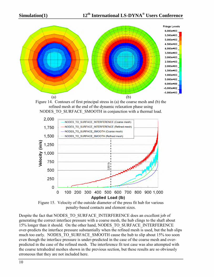
NODES_TO_SURFACE_INTERFERENCE. Unfortunately, the smooth embodiments of the interference contacts have not yet been implemented in LS-DYNA, so a different method of stress initialization has to be employed. The classic approach to this problem is to induce the preload via thermal expansion of the shaft and/or thermal contraction of the hub. NODES_TO_SURFACE_SMOOTH in conjunction with a thermal load produces an initial stress distribution very similar to the one generated by NODES_TO_SURFACE_INTERFERENCE (see Figure 14). Results from the torque application phase of the solution are presented in Figure 15 for both smooth and non-smooth contact.

Simulation(1) 12th


10

(a) (b)

Figure 14. Contours of first principal stress in (a) the coarse mesh and (b) the refined mesh at the end of the dynamic relaxation phase using

NODES_TO_SURFACE_SMOOTH in conjunction with a thermal load.

Figure 15. Velocity of the outside diameter of the press fit hub for various

penalty-based contacts and element sizes. Despite the fact that NODES_TO_SURFACE_INTERFERENCE does an excellent job of generating the correct interface pressure with a coarse mesh, the hub clings to the shaft about 15% longer than it should. On the other hand, NODES_TO_SURFACE_INTERFERENCE over-predicts the interface pressure substantially when the refined mesh is used, but the hub slips much too early. NODES_TO_SURFACE_SMOOTH cause the hub to slip about 15% too soon even though the interface pressure is under-predicted in the case of the coarse mesh and over-predicted in the case of the refined mesh. The interference fit test case was also attempted with the coarse tetrahedral meshes shown in the previous section, but these results are so obviously erroneous that they are not included here.

12th


11

Keyway Test Case

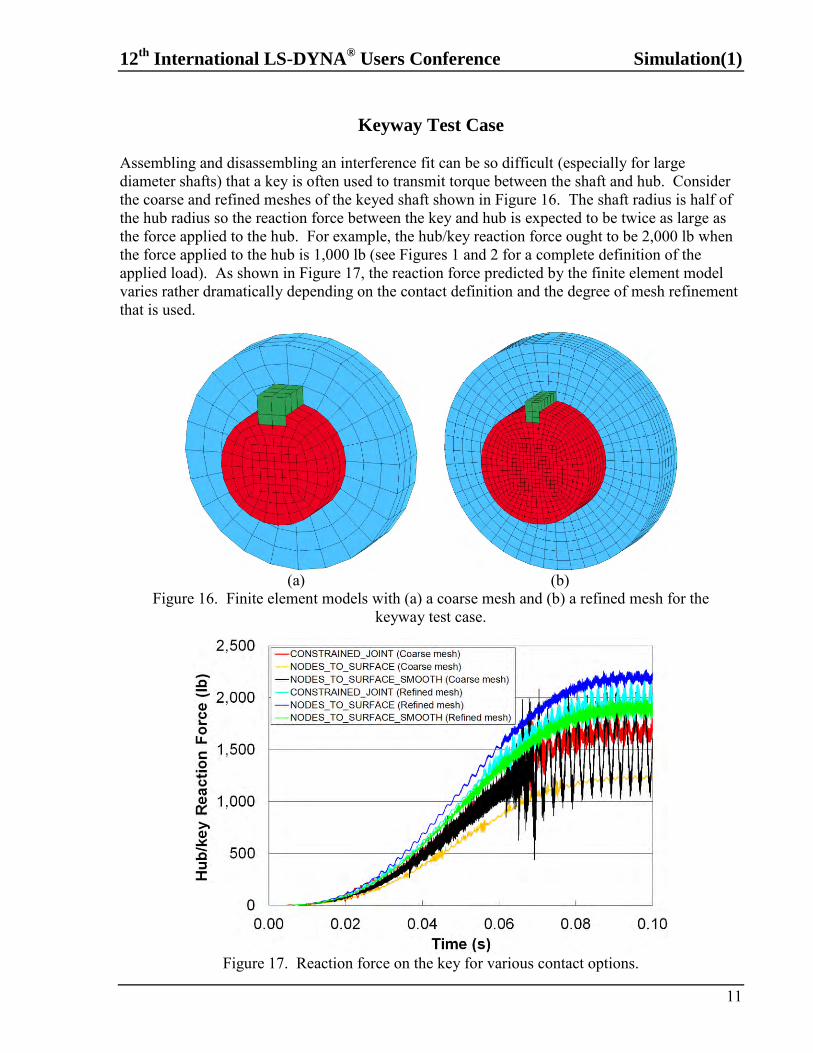
Assembling and disassembling an interference fit can be so difficult (especially for large diameter shafts) that a key is often used to transmit torque between the shaft and hub. Consider the coarse and refined meshes of the keyed shaft shown in Figure 16. The shaft radius is half of the hub radius so the reaction force between the key and hub is expected to be twice as large as the force applied to the hub. For example, the hub/key reaction force ought to be 2,000 lb when the force applied to the hub is 1,000 lb (see Figures 1 and 2 for a complete definition of the applied load). As shown in Figure 17, the reaction force predicted by the finite element model varies rather dramatically depending on the contact definition and the degree of mesh refinement that is used.

(a) (b)

Figure 16. Finite element models with (a) a coarse mesh and (b) a refined mesh for the keyway test case.

Figure 17. Reaction force on the key for various contact options.

Simulation(1) 12th


12

Summary and Conclusions The example problems presented in this paper demonstrate how mesh interlocking can make it difficult to correctly transfer torque between concentric cylindrical components in a finite element model. Fortunately, LS-DYNA provides a variety of methods for modeling contact interactions. The method that the user selects will depend on the specific requirements of the particular application, but the following guidelines and suggestions may be useful for problems that involve concentric cylinders:

Idealized joints and geometric contact entities are not susceptible to mesh interlocking, but require the components to be rigid. Even if rigid components are not acceptable for a particular application, idealized joints and geometric contact entities may be useful during model development for determining the correct load path in an assembly.

NODES_TO_SURFACE and ONE_WAY_SURFACE_TO_SURFACE are usually quite robust, especially when a relatively coarse mesh is employed. Either one is a good first choice when modeling concentric cylinders. SURFACE_TO_SURFACE contacts should be avoided in this application.

Smooth contacts perform remarkably well in certain situations, but they can also be more sensitive to small variations in the mesh than their non-smooth counterparts. It is recommended that smooth contact only be implemented after a model has been fully debugged with a non-smooth contact.

The default settings on the *CONTACT cards are usually adequate. Adjustments should only be required in situations such as contact between materials of dissimilar stiffness and/or mesh density.

The inner cylinder should always be the master surface in the contact definition. The master and slave nodes should be coincident in the contact region. Increasing the penalty stiffness scale factor increases the likelihood of mesh interlocking. It is very difficult to control the point at which an interference fit will slip. For a simple

interference fit, hand calculations are probably more reliable since the finite element solution may not be conservative. For more complicated situations such as load-sharing between an interference fit and a key, it may be wise to take the conservative approach of neglecting the torque carried by the interference fit.

As with any finite element solution, a mesh refinement study is recommended to determine the appropriate element size for a particular problem.

This study also led to the “development wish-list” shown below.

Implementation of *CONTACT…SMOOTH_INTERFERENCE. A way to visualize smooth contact surfaces in LS-PrePost (similar to the images in

reference [3]). A way to modify the curve fitting parameters used by the smooth contacts.

These developments would make smooth contact more user friendly, but would not necessarily eliminate the mesh interlocking problem. In order achieve that lofty goal a fundamental shift away from traditional polynomial-based finite element analysis as proposed by Hughes et al. [4] is probably required. Implementing NURBS-based isogeometric analysis is, perhaps, not justified by the mesh interlocking problem alone. Nevertheless, the contact treatments described by Temizer et al. [5] seem promising and may be the ideal approach to curved surface contact.

12th


13

References

[1] LS-DYNA Keyword User’s Manual version 971, Livermore Software Technology

Corporation, May 2007. [2] M. Lindeburg, Mechanical Engineering Reference Manual, Eleventh Edition, Professional

Publications, Inc. [3] X. Zhu “Smooth Contact” FEA Information, pp. 36–47, February 2008. [4] T. J. R. Hughes, J. A. Cottrell, and Y. Bazilevs “Isogeometric analysis: CAD, finite

elements, NURBS, exact geometry and mesh refinement,” Comput. Methods Appl. Mech. Engrg., 194:4135–4195.

[5] I. Temizer, P. Wriggers, and T.J.R. Hughes "Contact Treatment in Isogeometric Analysis

with NURBS", ICES REPORT 10-30, The Institute for Computational Engineering and Sciences, The University of Texas at Austin, July 2010.

Simulation(1) 12th


14

Documents

ISSN 2167-1273 Volume 1 Issue 9 October FEA Information Engineering Journal Information Engineering Journal... · Issue 9 . October. FEA Information Engineering Journal SIMULATION