1  

WWA A

11

Ho

If onwiTh

If ruexwecrintde

DeCrpomap

WWIIRREEBIMONTHND MINER

.. RReevviieewwow does the

we take a ven  two  thingsireline data,here has to b

we take a sinun  it  in a borxpect  to get e could  log oeating  somtersect someerives three i

Depth o

Thickne

Cross‐ho

epth  and  tross‐hole  coossible usingineral  log  dpply to most 

EELLIINNHLY BULLETRAL EXPLO

ww  ooff  ttwwoo  

e geologist be

ery simple los; depth con  that  the Y be, as well, a

ngle point rerehole  twicetwo very simother borehoething  of  vething intereimmediate b

of intersectio

ess of target 

ole correlati

hickness  arorrelation  is drill‐core daata‐set  is  baof the physi

NNEE WWTIN FOR WRATION 

yyeeaarrss  ‐‐  ss

enefit from t

og of formattrol and meaxis of  the  ln assumptio

esistance loge over a  twomilar  logs.  Ifoles with thevalue,  particesting, like a benefits from

on 

ion  

e  critical  os  pattern  rata. Much ofased  on  thecal property

WWOORRWIRELINE L

ssoommee  bboorr

the capture 

tion resistanasurement pog,  the depn of measur

, calibrate it o week periof  that  is  indee confidencecularly  if  th coal seam. T

m our efforts

objective  merecognition, f the value deese  three  bey logs. 

RRKKSSHHOGGERS A

rreehhoollee  lloo

of a geophy

ce, for instaprecision. Thth measuremement preci

in ohms, anod, we wouleed  the casee that we arhe  boreholeThe geologis: 

easurementsnot  alway

erived from enefits, whic

SPR l

HHOOPP AND GEOSC

 

 

 

 

 

 

 

 

 

 

ooggggiinngg  ffuu

ysical wirelin

nce, we can here has  to ment,  is accsion or repea

d d e, re es st 

s. ys a h 

T

A

og

CIENTISTS 

uunnddaammeenn

ne log? 

say that its be a valid aurate withinatability on t

Two‐Ye

Annive

The PE 

Transpo

Wirelin

A review

Issue 13 – Se

ENGAGED

nnttaallss

value depenssumption, n an acceptathe X axis of 

ear 

ersary Is

measurem

orting the

ne logging 

w of the l

eptember 201

D IN MININ

nds very muby  the user able  tolerancthe plot.  

ssue 

ment 

e unit 

basics 

ogs 

15 

NG 

ch of ce. 

2  

The data The wireline log is a graphic representation of continuous measurements that are  normally  stored  in  column  format.  As  the  depth wheel  on  the winch moves by one  log datum, usually 1 centimetre, a measurement  is recorded. Such an intensive sampling regime does not mean that the measurement has a resolution of 1 centimetre. A measurement at the tool's resolution, usually dependent on energy source to detector spacing,  is recorded at each depth datum. This is a bit like a moving average filter, where the filter length is the source‐detector  spacing.  Sampling  density  must  not  compromise  log resolution, so, given that file size  is no  longer an  issue for computer storage and processing  speed, 1  centimetre  (or an equivalent  in  feet)  is a practical standard. 

Column format data 

The three major benefits from a wireline log accrue even if the measurement is not calibrated (it is qualitative), although  long  term  precision  relies  on  some  form  of  normalisation where  at  least  the wiggly  line  appears somewhere on the page within a similar unit range. The human eye and the depth reference do the rest. 

Depth accuracy  Clearly, depth accuracy  is very  important, but  it  is often  taken  for granted. Both  logger and geologist  should recognise the need for depth measurement quality assurance during any logging programme. The provision of a test well  is a big advantage  in  this process but, otherwise, a  long  tape measure will do  the  job  if employed vertically while a sonde is lowered into a borehole. Depth errors are not always systematic. They can result from the logger misaligning his sonde depth datum with the geologist's surface datum, usually ground level, or failure to recheck that alignment on return to surface. 

The  depth  of  a  log  should  be  referenced  to  the  post‐log  check  against  the  surface datum because the up‐log is run with the logging cable tight on the depth wheel. 

Accuracy and precision One  oilfield  logging  commentator  stated  that  all mineral logs are qualitative in nature. While we have to commend  the Oilies  for  their ability  to cope with very  challenging  borehole  conditions,  we  can  say that,  because  mineral  borehole  conditions  are relatively benign, we do record accurate, quantitative measurements much of the time.  

As well as the three basic benefits of wireline logging for  minerals,  we  can  add,  at  the  very  least, quantitative  logs  of  coal  density,  iron  ore  density, uranium and potash grade based on natural gamma as well as excellent sonic  logs  for seismic calibration and very high resolution acoustic and optical images. 

Porosity is the key measurement in an oilfield play. It must  be  close  to  perfect.  That  is  not  the  case  in mineral  logging.  In  fact, we  are not much bothered about  absolute  porosity.  In  fact,  we  are  not  over concerned  about  the  absolute  accuracy  of many  of the  logs we produce...exceptions  include orientation data and sonic velocity. That might be an overstatement (of course) but the key to extracting value from mineral logs  is  very  often  empirically  based.  Beyond  depth,  thickness  and  correlation,  empiricism  is  the  critical  link between  a wiggly  line  and  valuable  extra  knowledge.  The  key  is  not  absolute  accuracy  but  precision. Most remote physical property measurements, which are estimations after all, cannot be perfectly accurate, but they must be precise, and can be made precise. Thereafter, conversion to site‐specific quantitative parameters such as coal ash percentage or uniaxial compressive strength or lab‐based bulk density should be straightforward. 

3  

The wireline  log  is,  at  least,  vertically  precise.  It  is  one  event. A  drill‐core  analysis comprises multiple events. 

Continuous, in‐situ, precise measurement offers the geologist and the mining engineer an objective framework on which to add subjective or laboratory‐based geological and geotechnical analyses. Where laboratory data are included, the continuous objective logs may be converted to more relevant parameters via empirical cross‐plot and regression. The wireline log tests the precision of laboratory measurement. 

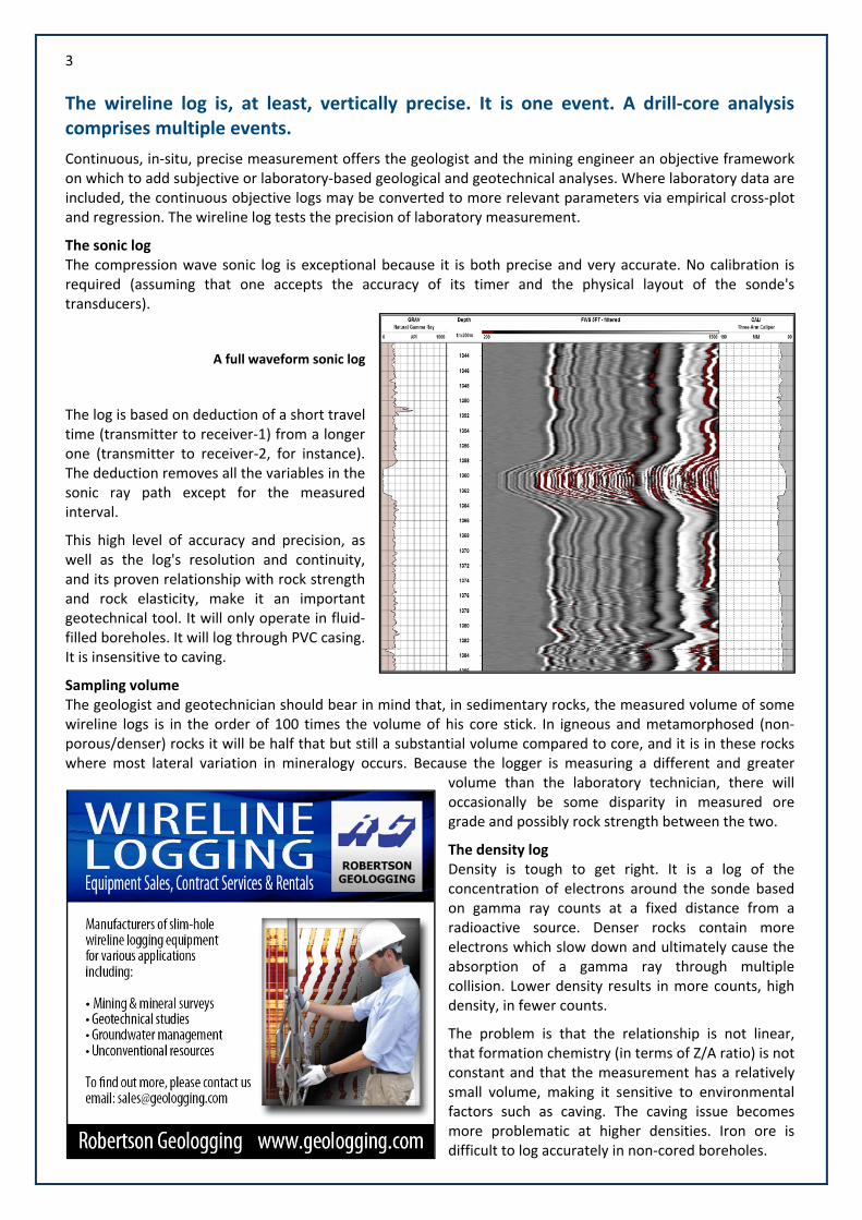
The sonic log The compression wave sonic  log  is exceptional because  it  is both precise and very accurate. No calibration  is required  (assuming  that  one  accepts  the  accuracy  of  its  timer  and  the  physical  layout  of  the  sonde's transducers). 

 

A full waveform sonic log 

 

The log is based on deduction of a short travel time (transmitter to receiver‐1) from a longer one  (transmitter  to  receiver‐2,  for  instance). The deduction removes all the variables in the sonic  ray  path  except  for  the  measured interval. 

This  high  level  of  accuracy  and  precision,  as well  as  the  log's  resolution  and  continuity, and its proven relationship with rock strength and  rock  elasticity,  make  it  an  important geotechnical tool. It will only operate in fluid‐filled boreholes. It will log through PVC casing. It is insensitive to caving. 

Sampling volume The geologist and geotechnician should bear in mind that, in sedimentary rocks, the measured volume of some wireline  logs  is  in  the order of 100  times  the volume of his core  stick.  In  igneous and metamorphosed  (non‐porous/denser) rocks it will be half that but still a substantial volume compared to core, and it is in these rocks where most  lateral  variation  in mineralogy  occurs.  Because  the  logger  is measuring  a  different  and  greater 

volume  than  the  laboratory  technician,  there  will occasionally  be  some  disparity  in  measured  ore grade and possibly rock strength between the two. 

The density log Density  is  tough  to  get  right.  It  is  a  log  of  the concentration of  electrons  around  the  sonde based on  gamma  ray  counts  at  a  fixed  distance  from  a radioactive  source.  Denser  rocks  contain  more electrons which slow down and ultimately cause the absorption  of  a  gamma  ray  through  multiple collision. Lower density  results  in more counts, high density, in fewer counts. 

The  problem  is  that  the  relationship  is  not  linear, that formation chemistry (in terms of Z/A ratio) is not constant and  that  the measurement has a relatively small  volume, making  it  sensitive  to  environmental factors  such  as  caving.  The  caving  issue  becomes more  problematic  at  higher  densities.  Iron  ore  is difficult to log accurately in non‐cored boreholes. 

4  

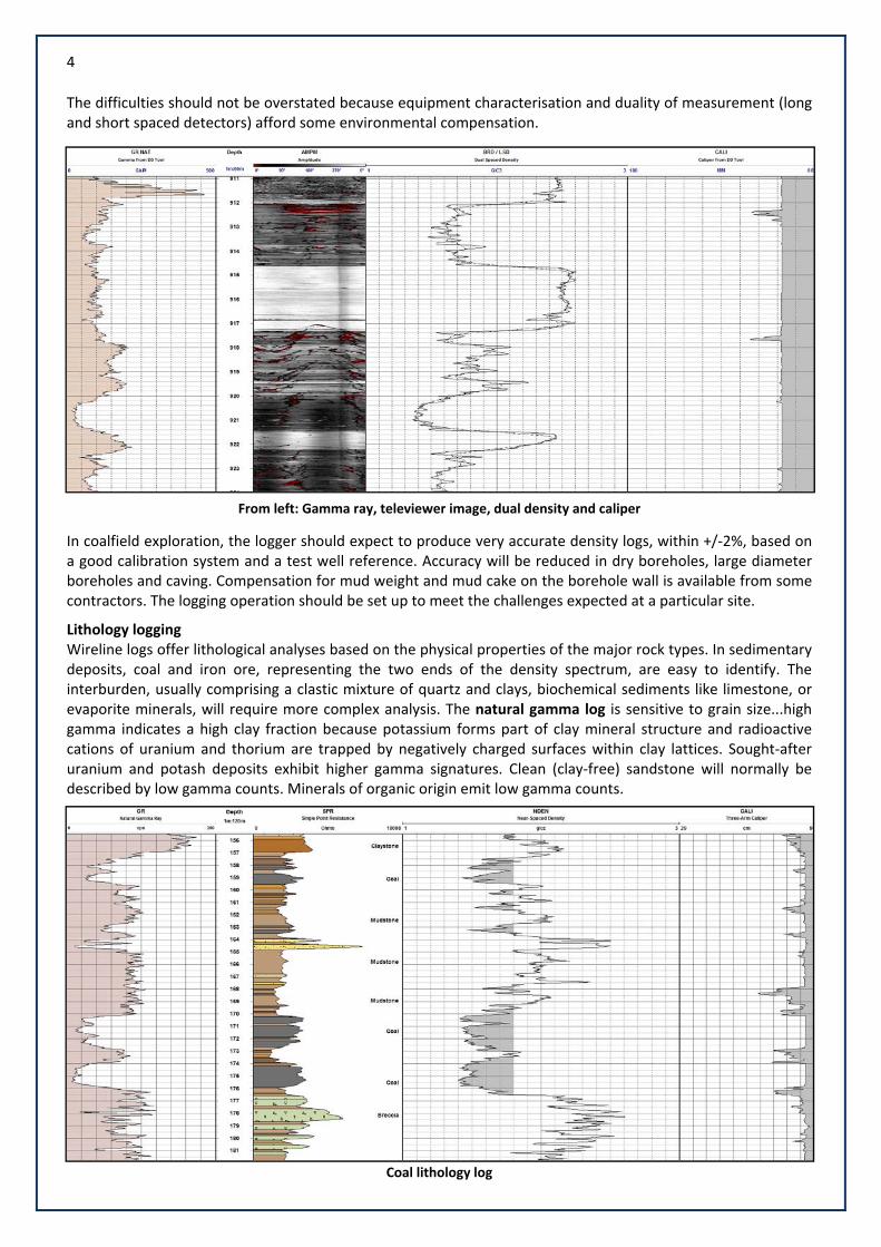
The difficulties should not be overstated because equipment characterisation and duality of measurement (long and short spaced detectors) afford some environmental compensation. 

From left: Gamma ray, televiewer image, dual density and caliper 

In coalfield exploration, the logger should expect to produce very accurate density logs, within +/‐2%, based on a good calibration system and a test well reference. Accuracy will be reduced  in dry boreholes,  large diameter boreholes and caving. Compensation for mud weight and mud cake on the borehole wall is available from some contractors. The logging operation should be set up to meet the challenges expected at a particular site. 

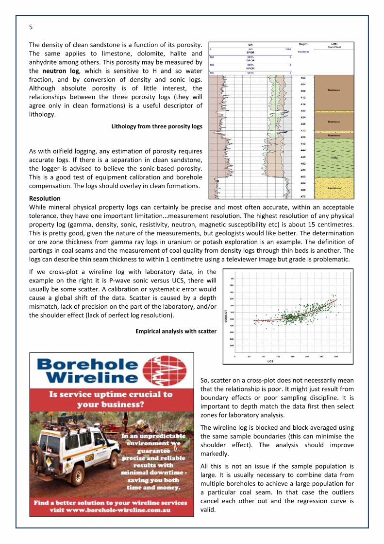
Lithology logging Wireline logs offer lithological analyses based on the physical properties of the major rock types. In sedimentary deposits,  coal  and  iron  ore,  representing  the  two  ends  of  the  density  spectrum,  are  easy  to  identify.  The interburden, usually comprising a clastic mixture of quartz and clays, biochemical sediments  like  limestone, or evaporite minerals, will require more complex analysis. The natural gamma  log  is sensitive to grain size...high gamma  indicates a high clay  fraction because potassium  forms part of clay mineral  structure and  radioactive cations of uranium and  thorium are  trapped by negatively  charged  surfaces within  clay  lattices. Sought‐after uranium  and  potash  deposits  exhibit  higher  gamma  signatures.  Clean  (clay‐free)  sandstone will  normally  be described by low gamma counts. Minerals of organic origin emit low gamma counts. 

Coal lithology log 

5  

The density of clean sandstone is a function of its porosity. The  same  applies  to  limestone,  dolomite,  halite  and anhydrite among others. This porosity may be measured by the  neutron  log,  which  is  sensitive  to  H  and  so  water fraction,  and  by  conversion  of  density  and  sonic  logs. Although  absolute  porosity  is  of  little  interest,  the relationships  between  the  three  porosity  logs  (they  will agree  only  in  clean  formations)  is  a  useful  descriptor  of lithology. 

Lithology from three porosity logs 

 

As with oilfield  logging, any estimation of porosity requires accurate  logs.  If  there  is  a  separation  in  clean  sandstone, the  logger  is  advised  to  believe  the  sonic‐based  porosity. This  is a good  test of equipment  calibration and borehole compensation. The logs should overlay in clean formations. 

Resolution While mineral physical property  logs  can  certainly be precise and most often accurate, within an acceptable tolerance, they have one important limitation...measurement resolution. The highest resolution of any physical property  log  (gamma, density, sonic,  resistivity, neutron, magnetic susceptibility etc)  is about 15 centimetres. This is pretty good, given the nature of the measurements, but geologists would like better. The determination or ore zone thickness  from gamma ray  logs  in uranium or potash exploration  is an example. The definition of partings in coal seams and the measurement of coal quality from density logs through thin beds is another. The logs can describe thin seam thickness to within 1 centimetre using a televiewer image but grade is problematic. 

If  we  cross‐plot  a  wireline  log  with  laboratory  data,  in  the example  on  the  right  it  is  P‐wave  sonic  versus UCS,  there will usually be some scatter. A calibration or systematic error would cause  a  global  shift  of  the  data.  Scatter  is  caused  by  a  depth mismatch, lack of precision on the part of the laboratory, and/or the shoulder effect (lack of perfect log resolution). 

Empirical analysis with scatter 

 

 

 

So, scatter on a cross‐plot does not necessarily mean that the relationship is poor. It might just result from boundary  effects  or  poor  sampling  discipline.  It  is important  to depth match  the data  first  then select zones for laboratory analysis.  

The wireline log is blocked and block‐averaged using the same sample boundaries  (this can minimise  the shoulder  effect).  The  analysis  should  improve markedly.  

All  this  is  not  an  issue  if  the  sample  population  is large.  It  is  usually  necessary  to  combine  data  from multiple boreholes to achieve a  large population for a  particular  coal  seam.  In  that  case  the  outliers cancel  each  other  out  and  the  regression  curve  is valid. 

6  

ReIn vosofofoma d 

  In tomphth

higde 

 

Threpaof

Thfracade

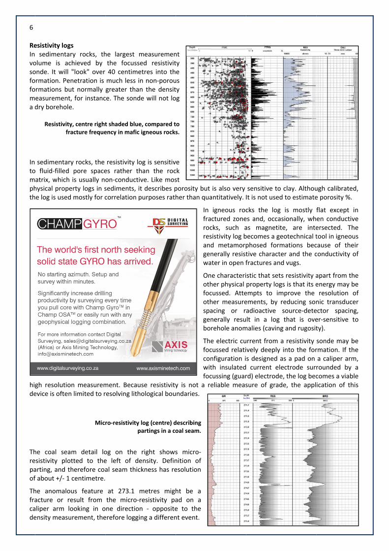
esistivity logsedimenta

olume  is  aconde.  It will rmation. Permations bueasurementdry borehole

Resistivityfr

sedimentaro  fluid‐filled atrix, which hysical propee log is used

gh  resolutioevice is often

he  coal  seaesistivity  ploarting, and tf about +/‐ 1 

he  anomaloacture  or  realiper  arm  loensity measu

gs ry  rocks,  thchieved  by "look" over netration  is ut normally , for  instance. 

y, centre rightacture freque

y rocks, the pore  spaceis usually noerty  logs  in sd mostly for c

on measuremn limited to r

Micr

am  detail  lootted  to  theherefore coacentimetre.

us  feature esult  from ooking  in  ourement, the

he  largest  mthe  focusse40  centimemuch  less  ingreater  thance. The sond

t shaded blueency in mafic 

resistivity loes  rather  thon‐conductivsediments,  itcorrelation p

ment.  Becauresolving lith

ro‐resistivity p

og  on  the e  left  of  deal seam thic 

at  273.1  mthe  micro‐rne  directionerefore loggi

measuremened  resistivitetres  into  thn non‐poroun  the densite will not  lo

e, compared tigneous rocks

og is sensitivhan  the  rocve. Like most describes ppurposes rath

se  resistivityological bou

log (centre) dpartings in a co

right  showsensity.  Definkness has re

metres  mighresistivity  pan  ‐  oppositeng a differen

nt ty e us ty og 

to s. 

ve ck st porosity buther than qua

In frarocresandgenwa

Onothfocothspagenbo

Thefocconwitfoc

y  is  not  a  rendaries. 

 describing oal seam. 

s  micro‐nition  of esolution 

ht  be  a ad  on  a e  to  the nt event. 

is also very antitatively. I

igneous  rocctured  zonecks,  such  asistivity log bd  metamorpnerally resistater in open f

ne characteriher physical cussed.  Atteher measureacing  or  rnerally  resurehole anom

e electric cucussed  relatinfiguration  ith  insulatedcussing (guareliable meas

sensitive to It is not used

cks  the  log es and, occaas  magnetitbecomes a gephosed  formtive charactefractures and

stic that setsproperty logempts  to  imements,  by  radioactive lt  in  a  log 

malies (caving

urrent from avely deeply s designed a  current  elerd) electrodesure  of  grad

clay. Althoud to estimate

is  mostly  fsionally, whte,  are  inteeotechnical tmations  becer and  the cd vugs. 

s resistivity ags is that its emprove  the reducing  sonsource‐detethat  is  oveg and rugosit

a resistivity into  the  foras a pad on ectrode  surre, the log becde,  the  appl

ugh calibratee porosity %.

flat  except en  conductiersected.  Ttool in igneocause  of  theconductivity 

apart from tenergy may resolution nic  transducector  spaciner‐sensitive ty).  

sonde may rmation.  If  tha caliper armrounded  by comes a viabication  of  th

ed, . 

in ve he us eir of 

he be of cer ng, to 

be he m, a 

ble his 

7  

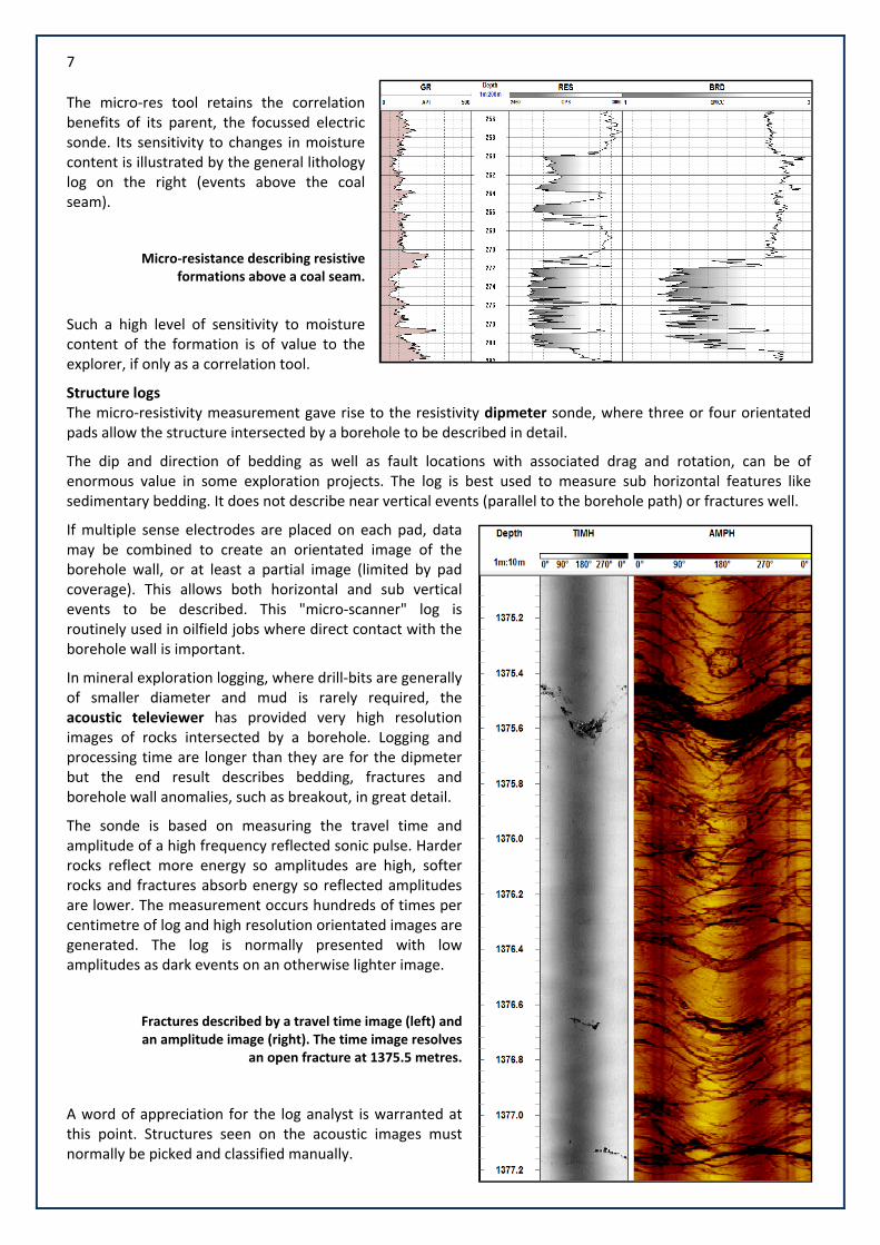
The  micro‐res  tool  retains  the  correlation benefits  of  its  parent,  the  focussed  electric sonde.  Its sensitivity  to changes  in moisture content is illustrated by the general lithology log  on  the  right  (events  above  the  coal seam). 

 

Micro‐resistance describing resistive formations above a coal seam. 

 

Such  a  high  level  of  sensitivity  to moisture content of  the  formation  is of  value  to  the explorer, if only as a correlation tool. 

Structure logs The micro‐resistivity measurement gave rise to the resistivity dipmeter sonde, where three or four orientated pads allow the structure intersected by a borehole to be described in detail. 

The  dip  and  direction  of  bedding  as  well  as  fault  locations  with  associated  drag  and  rotation,  can  be  of enormous  value  in  some  exploration  projects.  The  log  is  best  used  to measure  sub  horizontal  features  like sedimentary bedding. It does not describe near vertical events (parallel to the borehole path) or fractures well. 

If multiple  sense electrodes are placed on each pad, data may  be  combined  to  create  an  orientated  image  of  the borehole wall,  or  at  least  a  partial  image  (limited  by  pad coverage).  This  allows  both  horizontal  and  sub  vertical events  to  be  described.  This  "micro‐scanner"  log  is routinely used in oilfield jobs where direct contact with the borehole wall is important. 

In mineral exploration logging, where drill‐bits are generally of  smaller  diameter  and  mud  is  rarely  required,  the acoustic  televiewer  has  provided  very  high  resolution images  of  rocks  intersected  by  a  borehole.  Logging  and processing time are  longer than they are  for the dipmeter but  the  end  result  describes  bedding,  fractures  and borehole wall anomalies, such as breakout, in great detail. 

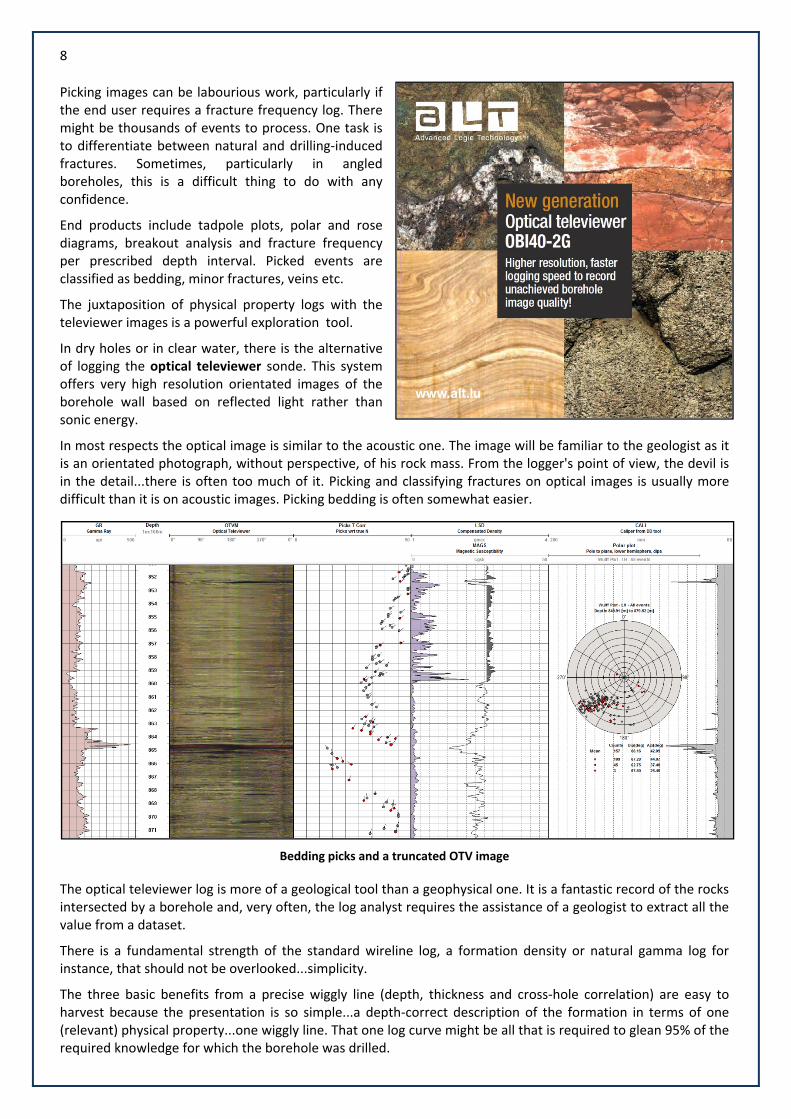
The  sonde  is  based  on  measuring  the  travel  time  and amplitude of a high frequency reflected sonic pulse. Harder rocks  reflect more  energy  so  amplitudes  are  high,  softer rocks and  fractures absorb energy so reflected amplitudes are lower. The measurement occurs hundreds of times per centimetre of log and high resolution orientated images are generated.  The  log  is  normally  presented  with  low amplitudes as dark events on an otherwise lighter image. 

 

Fractures described by a travel time image (left) and an amplitude image (right). The time image resolves 

an open fracture at 1375.5 metres. 

 

A word of appreciation  for  the  log analyst  is warranted at this  point.  Structures  seen  on  the  acoustic  images must normally be picked and classified manually. 

8  

Picking  images can be  labourious work, particularly  if the end user requires a fracture frequency  log. There might be thousands of events to process. One task  is to differentiate between natural and drilling‐induced fractures.  Sometimes,  particularly  in  angled boreholes,  this  is  a  difficult  thing  to  do  with  any confidence. 

End  products  include  tadpole  plots,  polar  and  rose diagrams,  breakout  analysis  and  fracture  frequency per  prescribed  depth  interval.  Picked  events  are classified as bedding, minor fractures, veins etc.  

The  juxtaposition  of  physical  property  logs with  the televiewer images is a powerful exploration  tool. 

In dry holes or  in clear water, there  is the alternative of  logging  the optical  televiewer  sonde. This  system offers  very  high  resolution  orientated  images  of  the borehole  wall  based  on  reflected  light  rather  than sonic energy. 

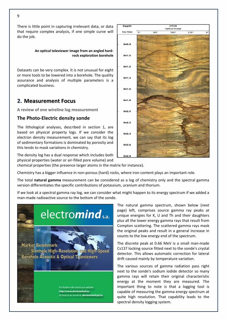
In most respects the optical image is similar to the acoustic one. The image will be familiar to the geologist as it is an orientated photograph, without perspective, of his rock mass. From the logger's point of view, the devil is in the detail...there  is often too much of  it. Picking and classifying  fractures on optical  images  is usually more difficult than it is on acoustic images. Picking bedding is often somewhat easier. 

Bedding picks and a truncated OTV image 

The optical televiewer log is more of a geological tool than a geophysical one. It is a fantastic record of the rocks intersected by a borehole and, very often, the log analyst requires the assistance of a geologist to extract all the value from a dataset. 

There  is  a  fundamental  strength of  the  standard wireline  log,  a  formation density or natural  gamma  log  for instance, that should not be overlooked...simplicity. 

The  three basic benefits  from  a precise wiggly  line  (depth,  thickness  and  cross‐hole  correlation)  are  easy  to harvest because  the presentation  is  so  simple...a depth‐correct description of  the  formation  in  terms of one (relevant) physical property...one wiggly line. That one log curve might be all that is required to glean 95% of the required knowledge for which the borehole was drilled. 

9  

There is little point in capturing irrelevant data, or data that  require  complex  analysis,  if one  simple  curve will do the job. 

 

An optical televiewer image from an angled hard‐rock exploration borehole 

 

Datasets can be very complex. It is not unusual for eight or more tools to be lowered into a borehole. The quality assurance  and  analysis  of  multiple  parameters  is  a complicated business. 

22.. MMeeaassuurreemmeenntt  FFooccuuss  

A review of one wireline log measurement 

The Photo‐Electric density sonde 

The  lithological  analyses,  described  in  section  1,  are based  on  physical  property  logs.  If  we  consider  the electron density measurement, we can  say  that  its  log of sedimentary formations is dominated by porosity and this tends to mask variations in chemistry.  

The density log has a dual response which includes both physical properties (water or air‐filled pore volume) and chemical properties (the presence larger atoms in the matrix for instance).  

Chemistry has a bigger influence in non‐porous (hard) rocks, where iron content plays an important role.  

The total natural gamma measurement can be considered as a  log of chemistry only and the spectral gamma version differentiates the specific contributions of potassium, uranium and thorium.  

If we look at a spectral gamma ray log, we can consider what might happen to its energy spectrum if we added a man‐made radioactive source to the bottom of the sonde.  

The  natural  gamma  spectrum,  shown  below  (next page)  left,  comprises  source  gamma  ray  peaks  at unique energies  for K, U and Th and  their daughters plus all the lower energy gamma rays that result from Compton scattering. The scattered gamma rays mask the original peaks and result  in a general  increase  in counts to the low energy end of the spectrum.  

The discrete peak at 0.66 MeV  is a  small man‐made Cs137 locking source fitted next to the sonde's crystal detector. This allows automatic correction for  lateral drift caused mainly by temperature variation.  

The  various  sources  of  gamma  radiation  pass  right next  to  the sonde's sodium  iodide detector so many gamma  rays  will  retain  their  original  characteristic energy  at  the  moment  they  are  measured.  The important  thing  to  note  is  that  a  logging  tool  is capable of measuring the gamma energy spectrum at quite  high  resolution.  That  capability  leads  to  the spectral density logging system. 

10  

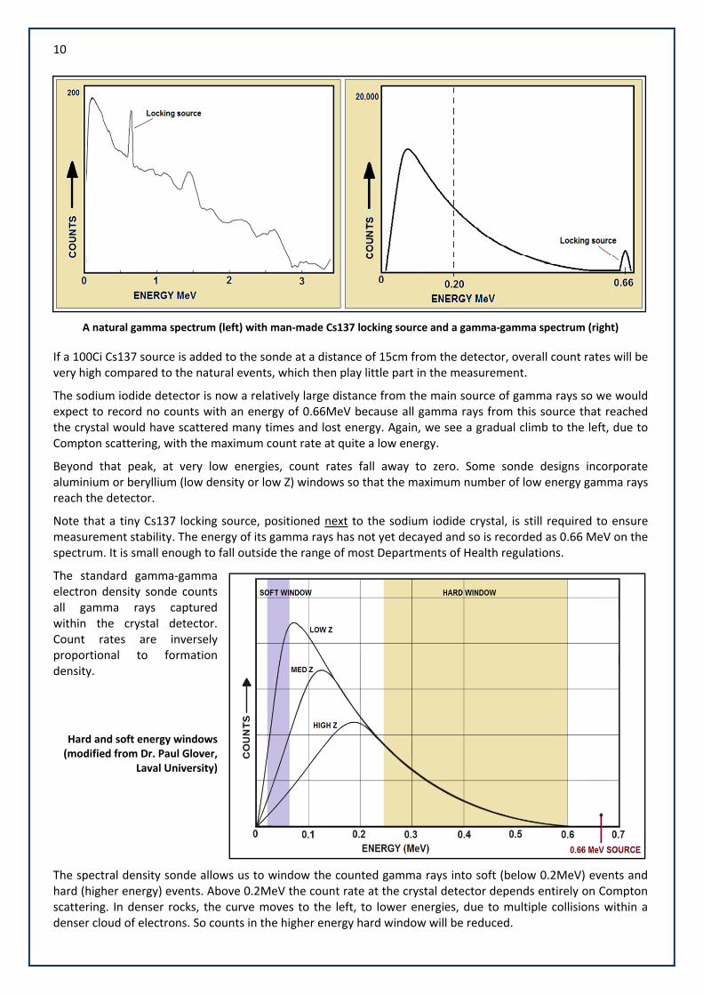
A natural gamma spectrum (left) with man‐made Cs137 locking source and a gamma‐gamma spectrum (right) 

If a 100Ci Cs137 source is added to the sonde at a distance of 15cm from the detector, overall count rates will be very high compared to the natural events, which then play little part in the measurement.  

The sodium iodide detector is now a relatively large distance from the main source of gamma rays so we would expect to record no counts with an energy of 0.66MeV because all gamma rays from this source that reached the crystal would have scattered many times and lost energy. Again, we see a gradual climb to the left, due to Compton scattering, with the maximum count rate at quite a low energy.  

Beyond  that  peak,  at  very  low  energies,  count  rates  fall  away  to  zero.  Some  sonde  designs  incorporate aluminium or beryllium (low density or low Z) windows so that the maximum number of low energy gamma rays reach the detector. 

Note that a tiny Cs137  locking source, positioned next  to the sodium  iodide crystal,  is still required  to ensure measurement stability. The energy of its gamma rays has not yet decayed and so is recorded as 0.66 MeV on the spectrum. It is small enough to fall outside the range of most Departments of Health regulations. 

The  standard  gamma‐gamma electron density  sonde  counts all  gamma  rays  captured within  the  crystal  detector. Count  rates  are  inversely proportional  to  formation density.  

 

 

Hard and soft energy windows (modified from Dr. Paul Glover, 

Laval University) 

 

 

 

 The spectral density sonde allows us to window the counted gamma rays into soft (below 0.2MeV) events and hard (higher energy) events. Above 0.2MeV the count rate at the crystal detector depends entirely on Compton scattering.  In denser  rocks,  the curve moves  to  the  left,  to  lower energies, due  to multiple collisions within a denser cloud of electrons. So counts in the higher energy hard window will be reduced. 

11  

Below  0.2MeV,  the  count  rate  depends  on  both  Compton scattering  and photo‐absorption by  atoms  in  the  formation. At such low energies, gamma rays are available for absorption by  any  elemental  atom  but  some  elements  have  higher photo‐electric  absorption  capacities  (cross‐sections)  than others.  Elements  of  higher  Z  (more  protons),  having more tightly bound electrons, tend to have higher absorption cross‐sections than those with lower Z.  

So the count rate  in the soft window  is partly dependent on the average Z of the  logged formation. The ratio S/H, soft to hard window, will be a function of the Z effect only. 

In  uranium  logging,  the  measurement  of  natural  gamma radiation  requires  correction  for  the  same phenomenon.  In that case, the uranium family of relatively huge atoms in the formation have a large absorption cross‐section and, at high U grade,  the  formation actually absorbs a proportion of  its own  gamma  rays  (from  the  various  daughter  isotopes) before they can reach the sonde.  

The  natural  gamma  log  understates  daughter  counts,  and therefore  derived  U  grade.  Correction,  based  on  empirical trials in assayed rocks or jigs, is required. 

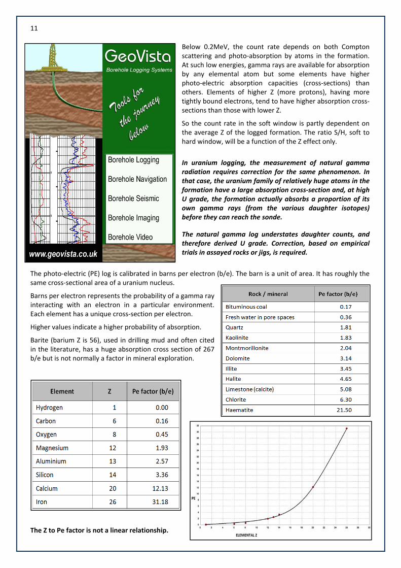
The photo‐electric (PE) log is calibrated in barns per electron (b/e). The barn is a unit of area. It has roughly the same cross‐sectional area of a uranium nucleus.  

Barns per electron represents the probability of a gamma ray interacting  with  an  electron  in  a  particular  environment. Each element has a unique cross‐section per electron.  

Higher values indicate a higher probability of absorption. 

Barite (barium Z  is 56), used  in drilling mud and often cited in the  literature, has a huge absorption cross section of 267 b/e but is not normally a factor in mineral exploration. 

  

 

 

 The Z to Pe factor is not a linear relationship. 

12  

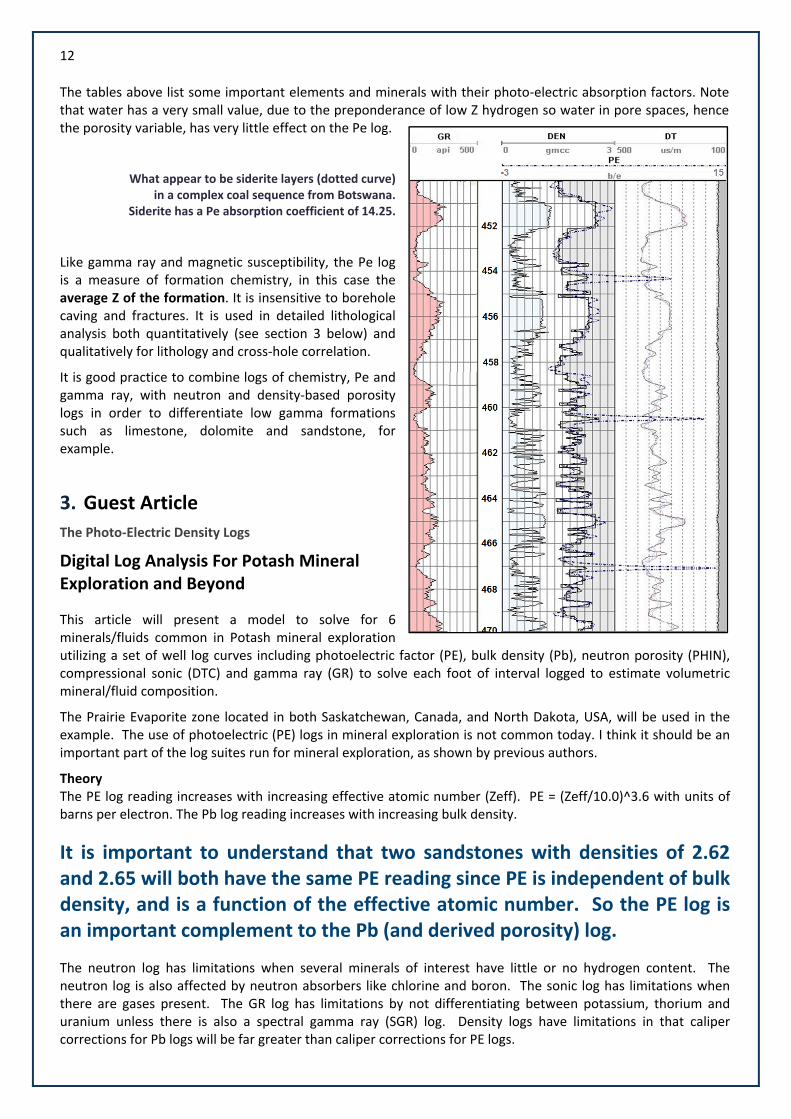
The tables above list some important elements and minerals with their photo‐electric absorption factors. Note that water has a very small value, due to the preponderance of low Z hydrogen so water in pore spaces, hence the porosity variable, has very little effect on the Pe log. 

 

What appear to be siderite layers (dotted curve) in a complex coal sequence from Botswana. 

Siderite has a Pe absorption coefficient of 14.25. 

 

Like gamma ray and magnetic susceptibility,  the Pe  log is  a measure  of  formation  chemistry,  in  this  case  the average Z of the formation. It is insensitive to borehole caving  and  fractures.  It  is  used  in  detailed  lithological analysis  both  quantitatively  (see  section  3  below)  and qualitatively for lithology and cross‐hole correlation. 

It is good practice to combine logs of chemistry, Pe and gamma  ray,  with  neutron  and  density‐based  porosity logs  in  order  to  differentiate  low  gamma  formations such  as  limestone,  dolomite  and  sandstone,  for example. 

3. Guest Article The Photo‐Electric Density Logs 

Digital Log Analysis For Potash Mineral Exploration and Beyond 

This  article  will  present  a  model  to  solve  for  6 minerals/fluids  common  in  Potash mineral  exploration utilizing a set of well  log curves  including photoelectric factor (PE), bulk density (Pb), neutron porosity (PHIN), compressional  sonic  (DTC)  and  gamma  ray  (GR)  to  solve each  foot of  interval  logged  to  estimate  volumetric mineral/fluid composition.   

The Prairie Evaporite zone  located  in both Saskatchewan, Canada, and North Dakota, USA, will be used  in the example.  The use of photoelectric (PE) logs in mineral exploration is not common today. I think it should be an important part of the log suites run for mineral exploration, as shown by previous authors.  

Theory The PE  log reading  increases with  increasing effective atomic number (Zeff).   PE = (Zeff/10.0)^3.6 with units of barns per electron. The Pb log reading increases with increasing bulk density.  

It  is  important  to understand  that  two  sandstones with densities of 2.62 and 2.65 will both have the same PE reading since PE is independent of bulk density, and is a function of the effective atomic number.   So the PE log is an important complement to the Pb (and derived porosity) log. 

The  neutron  log  has  limitations when  several minerals  of  interest  have  little  or  no  hydrogen  content.    The neutron  log  is also affected by neutron absorbers  like chlorine and boron.   The sonic  log has  limitations when there  are  gases present.    The GR  log has  limitations by not differentiating between potassium,  thorium  and uranium  unless  there  is  also  a  spectral  gamma  ray  (SGR)  log.    Density  logs  have  limitations  in  that  caliper corrections for Pb logs will be far greater than caliper corrections for PE logs.  

13  

PE logs can also be made more valuable by creating mathematical relationships between the PE reading and Pb reading  for  selected minerals which provide  additional measurements of  lithology.   Techniques  such  as M‐N Lithology can be enhanced to use PE data to replace PHIN data  in their equations.   Similarly, MID plots can be utilized  to  create  additional  equations  for  various minerals  and  fluids.  I  have  also  developed  an  alternative method that currently solves for 29 minerals/fluids with a great deal of accuracy. 

Example The well log data in a 6 mineral/fluid model can be solved as a set of simultaneous linear equations.  Since there are 5  log measurements, plus a unity equation, then we can solve for 6 unknowns (minerals/fluids).   The unity equation simply states that the sum of the individual volumetric mineral/fluids fractions is equal to one.  Since reservoir rocks are complex mixtures of minerals/fluids, a rigorous solution will require including far more than 6 minerals/fluids  in  the  analysis.   However,  the  purpose  of  this  article  is  to  present  a  simplified  technique  to estimate mineral/fluid composition for a six mineral/fluid model. 

A key part of a successful analysis  is to first  identify the most common minerals/fluids present  in the zone you are analyzing.    In a  typical potash zone  the most common minerals/fluids are NaCl, KCl, Carnallite, Anhydrite, Clay and Water/Brine.  These will be used in our example.  

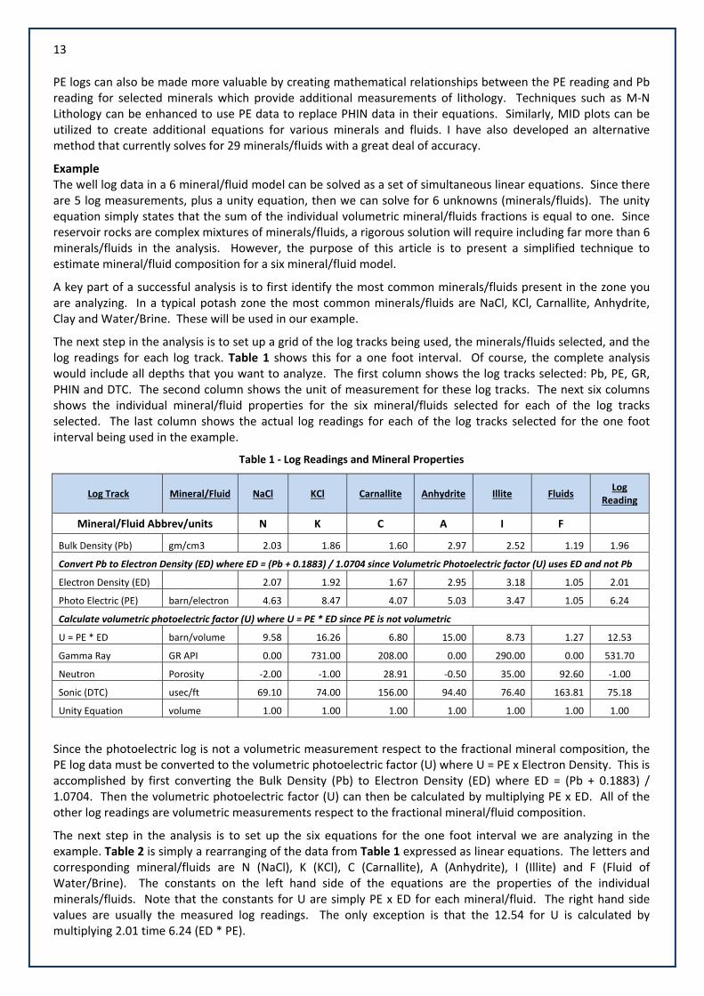
The next step in the analysis is to set up a grid of the log tracks being used, the minerals/fluids selected, and the log  readings  for each  log  track. Table 1  shows  this  for a one  foot  interval.   Of  course,  the  complete analysis would  include all depths that you want to analyze.   The first column shows the  log tracks selected: Pb, PE, GR, PHIN and DTC.  The second column shows the unit of measurement for these log tracks.  The next six columns shows  the  individual mineral/fluid  properties  for  the  six mineral/fluids  selected  for  each  of  the  log  tracks selected.   The  last column  shows  the actual  log  readings  for each of  the  log  tracks  selected  for  the one  foot interval being used in the example.  

Table 1 ‐ Log Readings and Mineral Properties 

 Log Track  Mineral/Fluid  NaCl  KCl  Carnallite  Anhydrite  Illite  Fluids Log 

Reading 

Mineral/Fluid Abbrev/units  N  K  C  A  I  F 

Bulk Density (Pb)  gm/cm3   2.03  1.86  1.60  2.97  2.52  1.19  1.96 

Convert Pb to Electron Density (ED) where ED = (Pb + 0.1883) / 1.0704 since Volumetric Photoelectric factor (U) uses ED and not Pb 

Electron Density (ED)     2.07  1.92  1.67  2.95  3.18  1.05  2.01 

Photo Electric (PE)  barn/electron   4.63  8.47  4.07  5.03  3.47  1.05  6.24 

Calculate volumetric photoelectric factor (U) where U = PE * ED since PE is not volumetric 

U = PE * ED  barn/volume  9.58  16.26  6.80  15.00  8.73  1.27  12.53 

Gamma Ray  GR API   0.00  731.00  208.00  0.00  290.00  0.00  531.70 

Neutron   Porosity   ‐2.00  ‐1.00  28.91  ‐0.50  35.00  92.60  ‐1.00 

Sonic (DTC)  usec/ft   69.10  74.00  156.00  94.40  76.40  163.81  75.18 

Unity Equation  volume  1.00  1.00  1.00  1.00  1.00  1.00  1.00 

 

Since the photoelectric log is not a volumetric measurement respect to the fractional mineral composition, the PE log data must be converted to the volumetric photoelectric factor (U) where U = PE x Electron Density.  This is accomplished  by  first  converting  the Bulk Density  (Pb)  to  Electron Density  (ED) where  ED  =  (Pb  +  0.1883)  / 1.0704.   Then the volumetric photoelectric factor (U) can then be calculated by multiplying PE x ED.   All of the other log readings are volumetric measurements respect to the fractional mineral/fluid composition. 

The next  step  in  the analysis  is  to  set up  the  six equations  for  the one  foot  interval we are analyzing  in  the example. Table 2 is simply a rearranging of the data from Table 1 expressed as linear equations.  The letters and corresponding  mineral/fluids  are  N  (NaCl),  K  (KCl),  C  (Carnallite),  A  (Anhydrite),  I  (Illite)  and  F  (Fluid  of Water/Brine).    The  constants  on  the  left  hand  side  of  the  equations  are  the  properties  of  the  individual minerals/fluids.   Note that the constants  for U are simply PE x ED  for each mineral/fluid.   The right hand side values  are  usually  the measured  log  readings.    The  only  exception  is  that  the  12.54  for  U  is  calculated  by multiplying 2.01 time 6.24 (ED * PE).   

14  

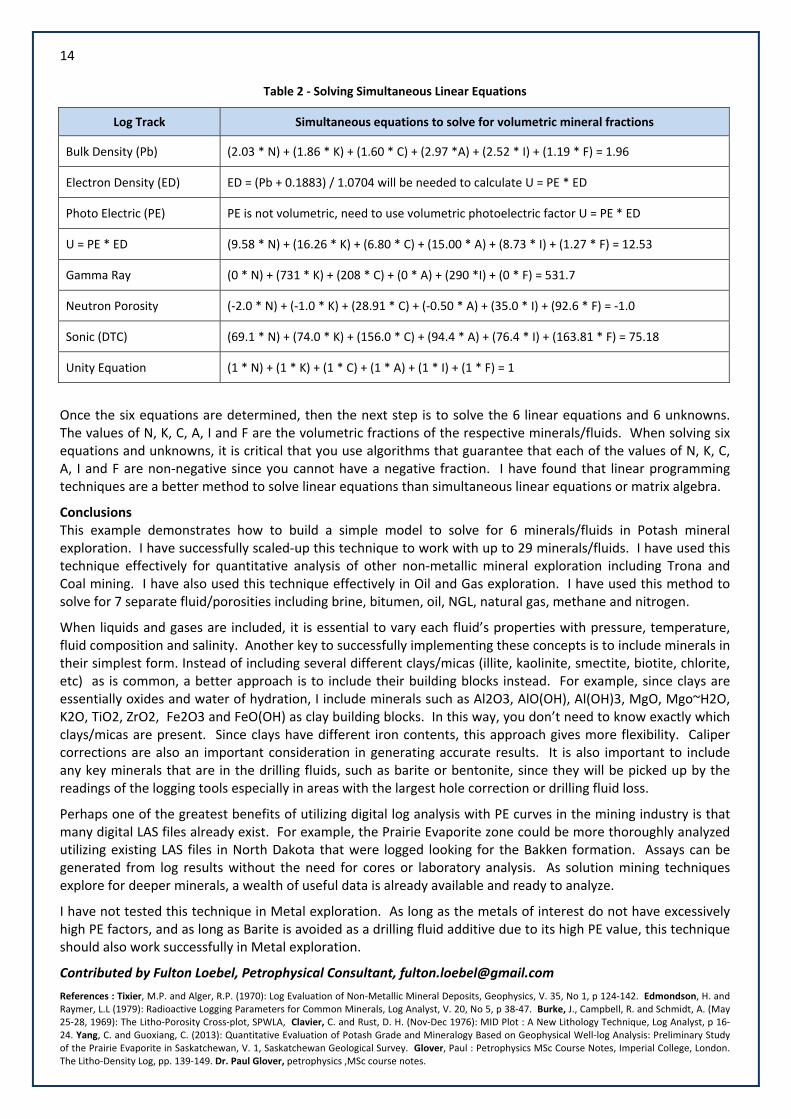
Table 2 ‐ Solving Simultaneous Linear Equations 

Log Track  Simultaneous equations to solve for volumetric mineral fractions 

Bulk Density (Pb)  (2.03 * N) + (1.86 * K) + (1.60 * C) + (2.97 *A) + (2.52 * I) + (1.19 * F) = 1.96 

Electron Density (ED)  ED = (Pb + 0.1883) / 1.0704 will be needed to calculate U = PE * ED 

Photo Electric (PE)  PE is not volumetric, need to use volumetric photoelectric factor U = PE * ED 

U = PE * ED  (9.58 * N) + (16.26 * K) + (6.80 * C) + (15.00 * A) + (8.73 * I) + (1.27 * F) = 12.53 

Gamma Ray  (0 * N) + (731 * K) + (208 * C) + (0 * A) + (290 *I) + (0 * F) = 531.7 

Neutron Porosity  (‐2.0 * N) + (‐1.0 * K) + (28.91 * C) + (‐0.50 * A) + (35.0 * I) + (92.6 * F) = ‐1.0 

Sonic (DTC)  (69.1 * N) + (74.0 * K) + (156.0 * C) + (94.4 * A) + (76.4 * I) + (163.81 * F) = 75.18 

Unity Equation  (1 * N) + (1 * K) + (1 * C) + (1 * A) + (1 * I) + (1 * F) = 1 

 

Once the six equations are determined, then the next step  is to solve the 6  linear equations and 6 unknowns.  The values of N, K, C, A, I and F are the volumetric fractions of the respective minerals/fluids.  When solving six equations and unknowns, it is critical that you use algorithms that guarantee that each of the values of N, K, C, A,  I and F are non‐negative since you cannot have a negative  fraction.    I have  found  that  linear programming techniques are a better method to solve linear equations than simultaneous linear equations or matrix algebra.    

Conclusions This  example  demonstrates  how  to  build  a  simple model  to  solve  for  6 minerals/fluids  in  Potash mineral exploration.  I have successfully scaled‐up this technique to work with up to 29 minerals/fluids.  I have used this technique  effectively  for  quantitative  analysis  of  other  non‐metallic mineral  exploration  including  Trona  and Coal mining.  I have also used this technique effectively in Oil and Gas exploration.  I have used this method to solve for 7 separate fluid/porosities including brine, bitumen, oil, NGL, natural gas, methane and nitrogen.  

When  liquids and gases are  included,  it  is essential to vary each fluid’s properties with pressure, temperature, fluid composition and salinity.  Another key to successfully implementing these concepts is to include minerals in their simplest form. Instead of including several different clays/micas (illite, kaolinite, smectite, biotite, chlorite, etc)   as  is common, a better approach  is to  include their building blocks  instead.   For example, since clays are essentially oxides and water of hydration, I include minerals such as Al2O3, AlO(OH), Al(OH)3, MgO, Mgo~H2O, K2O, TiO2, ZrO2,  Fe2O3 and FeO(OH) as clay building blocks.  In this way, you don’t need to know exactly which clays/micas are present.   Since clays have different  iron contents, this approach gives more flexibility.   Caliper corrections are also an  important consideration  in generating accurate results.    It  is also  important  to  include any key minerals that are  in the drilling fluids, such as barite or bentonite, since they will be picked up by the readings of the logging tools especially in areas with the largest hole correction or drilling fluid loss.   

Perhaps one of the greatest benefits of utilizing digital log analysis with PE curves in the mining industry is that many digital LAS files already exist.  For example, the Prairie Evaporite zone could be more thoroughly analyzed utilizing existing LAS  files  in North Dakota  that were  logged  looking  for  the Bakken  formation.   Assays can be generated  from  log  results without  the need  for  cores or  laboratory analysis.   As  solution mining  techniques explore for deeper minerals, a wealth of useful data is already available and ready to analyze.   

I have not tested this technique in Metal exploration.  As long as the metals of interest do not have excessively high PE factors, and as long as Barite is avoided as a drilling fluid additive due to its high PE value, this technique should also work successfully in Metal exploration. 

Contributed by Fulton Loebel, Petrophysical Consultant, fulton.loebel@gmail.com 

References : Tixier, M.P. and Alger, R.P. (1970): Log Evaluation of Non‐Metallic Mineral Deposits, Geophysics, V. 35, No 1, p 124‐142.  Edmondson, H. and Raymer, L.L (1979): Radioactive Logging Parameters for Common Minerals, Log Analyst, V. 20, No 5, p 38‐47.  Burke, J., Campbell, R. and Schmidt, A. (May 25‐28, 1969): The Litho‐Porosity Cross‐plot, SPWLA,  Clavier, C. and Rust, D. H. (Nov‐Dec 1976): MID Plot : A New Lithology Technique, Log Analyst, p 16‐24. Yang, C. and Guoxiang, C. (2013): Quantitative Evaluation of Potash Grade and Mineralogy Based on Geophysical Well‐log Analysis: Preliminary Study of the Prairie Evaporite in Saskatchewan, V. 1, Saskatchewan Geological Survey.  Glover, Paul : Petrophysics MSc Course Notes, Imperial College, London. The Litho‐Density Log, pp. 139‐149. Dr. Paul Glover, petrophysics ,MSc course notes. 

15  

4. The Logger on Site Where there's a will... 

Some fun with transporting equipment 

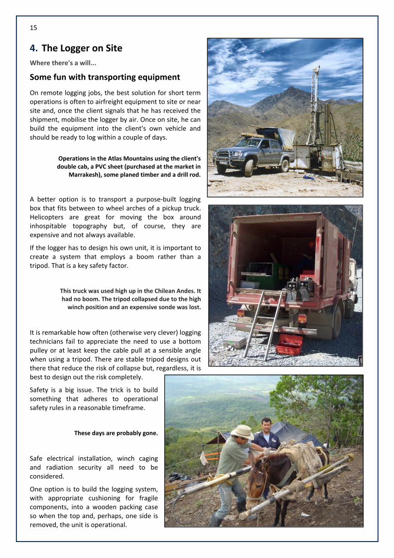
On remote  logging  jobs, the best solution for short term operations is often to airfreight equipment to site or near site and, once the client signals that he has received the shipment, mobilise the logger by air. Once on site, he can build  the  equipment  into  the  client's  own  vehicle  and should be ready to log within a couple of days.    

Operations in the Atlas Mountains using the client's double cab, a PVC sheet (purchased at the market in 

Marrakesh), some planed timber and a drill rod. 

 

A  better  option  is  to  transport  a  purpose‐built  logging box that fits between to wheel arches of a pickup truck. Helicopters  are  great  for  moving  the  box  around inhospitable  topography  but,  of  course,  they  are expensive and not always available. 

If the logger has to design his own unit, it is important to create  a  system  that  employs  a  boom  rather  than  a tripod. That is a key safety factor. 

 

This truck was used high up in the Chilean Andes. It had no boom. The tripod collapsed due to the high winch position and an expensive sonde was lost. 

 

It is remarkable how often (otherwise very clever) logging technicians  fail  to appreciate  the need  to use a bottom pulley or at  least keep  the cable pull at a sensible angle when using a tripod. There are stable tripod designs out there that reduce the risk of collapse but, regardless, it is best to design out the risk completely. 

Safety  is  a  big  issue.  The  trick  is  to  build something  that  adheres  to  operational safety rules in a reasonable timeframe. 

 

These days are probably gone. 

 

Safe  electrical  installation,  winch  caging and  radiation  security  all  need  to  be considered. 

One option  is  to build  the  logging system, with  appropriate  cushioning  for  fragile components,  into  a wooden  packing  case so when the top and, perhaps, one side  is removed, the unit is operational. 

16  

55.. WWiirreelliinnee  ddaattaa  pprroocceessssiinngg  aanndd  aannaallyyssiiss  

How to get the best from the logs 

Objectivity in fracture frequency logs 

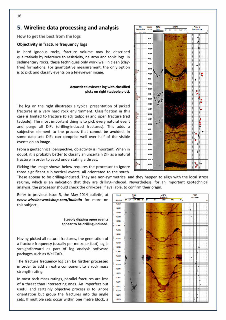
In  hard  igneous  rocks,  fracture  volume  may  be  described qualitatively by reference to resistivity, neutron and sonic logs. In sedimentary rocks, these techniques only work well in clean (clay‐free)  formations. For quantitative measurement,  the only option is to pick and classify events on a televiewer image. 

 

Acoustic televiewer log with classified picks on right (tadpole plot). 

 

The  log  on  the  right  illustrates  a  typical  presentation  of  picked fractures  in  a  very  hard  rock  environment.  Classification  in  this case  is  limited to  fracture  (black  tadpole) and open  fracture  (red tadpole). The most  important thing  is to pick every natural event and  purge  all  DIFs  (drilling‐induced  fractures).  This  adds  a subjective  element  to  the  process  that  cannot  be  avoided.  In some  data  sets  DIFs  can  comprise well  over  half  of  the  visible events on an image. 

From a geotechnical perspective, objectivity is important. When in doubt, it is probably better to classify an uncertain DIF as a natural fracture in order to avoid understating a threat. 

Picking  the  image shown below  requires  the processor  to  ignore three  significant  sub vertical events, all orientated  to  the  south. These appear  to be drilling‐induced. They are non‐symmetrical and  they happen  to align with  the  local stress regime,  which  is  an  indication  that  they  are  drilling‐induced.  Nevertheless,  for  an  important  geotechnical analysis, the processor should check the drill‐core, if available, to confirm their origin. 

Refer  to previous  issue 5,  the May 2014 bulletin, at www.wirelineworkshop.com/bulletin  for  more  on this subject. 

 

Steeply dipping open events appear to be drilling‐induced. 

 

Having picked all natural fractures, the generation of a fracture frequency (usually per metre or foot) log is straightforward  as  part  of  log  analysis  software packages such as WellCAD. 

The  fracture  frequency  log can be  further processed in order  to add an extra component  to a  rock mass strength rating. 

In most  rock mass  ratings, parallel  fractures are  less of a  threat  than  intersecting ones. An  imperfect but useful  and  certainly  objective  process  is  to  ignore orientation  but  group  the  fractures  into  dip  angle sets. If multiple sets occur within one metre block, a 

17  

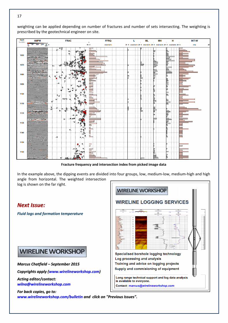
weighting can be applied depending on number of fractures and number of sets  intersecting. The weighting  is prescribed by the geotechnical engineer on site. 

Fracture frequency and intersection index from picked image data 

In the example above, the dipping events are divided into four groups, low, medium‐low, medium‐high and high angle  from  horizontal.  The  weighted  intersection log is shown on the far right. 

 

NNeexxtt  IIssssuuee::  

Fluid logs and formation temperature 

 

 

 

  

  

MMaarrccuuss  CChhaattffiieelldd  ––  SSeepptteemmbbeerr  22001155  

CCooppyyrriigghhttss  aappppllyy  ((wwwwww..wwiirreelliinneewwoorrkksshhoopp..ccoomm))  

AAccttiinngg  eeddiittoorr//ccoonnttaacctt::  

wwiillnnaa@@wwiirreelliinneewwoorrkksshhoopp..ccoomm  

FFoorr  bbaacckk  ccooppiieess,,  ggoo  ttoo::  

wwwwww..wwiirreelliinneewwoorrkksshhoopp..ccoomm//bbuulllleettiinn  aanndd    cclliicckk  oonn  ""PPrreevviioouuss  IIssssuueess""..