ISSUES RELATED TO SPORTS GAMBLING

Robin Insley, Lucia Mok and Tim Swartz ∗

Summary

This paper looks at various issues that are of interest to the sports gambler. First, an

expression is obtained for the distribution of the final bankroll using fixed wagers with

a specified initial bankroll. Second, fixed percentage wagers are considered where the

Kelly method is extended to the case of simultaneous bets placed at various odds; a

computational algorithm is presented to obtain the Kelly fractions. Finally, we consider

the problem of determining whether a gambling system is profitable based on the historical

results of bets placed at various odds.

Key words: gambler’s ruin, Kelly method, optimal wagering, comparative inference, Gibbs

sampling, meta-analysis.

1. Introduction

Despite its illegality in many jurisdictions, gambling on the outcome of sporting events

is a common activity. For example, Crist (1998) states that Americans illegally wager

∗Robin Insley is Senior Lecturer, Lucia Mok is an MSc graduate and Tim Swartz is Professor, De-partment of Statistics and Actuarial Science, Simon Fraser University, Burnaby BC, Canada V5A1S6.Swartz’s work was partially supported by a grant from the Natural Sciences and Engineering ResearchCouncil of Canada. The authors thank an Associate Editor and two referees whose comments lead to animprovement in the manuscript.

1

over $100 billion annually on professional and college sports. On the 1999 Superbowl

(the championship game of the National Football League), approximately $87 million

was wagered legally in Las Vegas Sportsbooks (Ordine, 2000). In Australia, commercial

gambling on racing alone (horses and greyhounds) resulted in individual losses of $1.6

billion in 1997-1998 (Productivity Commission, 1999).

Sports gambling has been increasing over the years (Productivity Commission, 1999)

and it is likely that the trend will continue as more government bodies are eager to share

in the huge profits that have and can be made. One particular avenue for growth is sports

gambling via the internet (Haywood, 2000). Whereas such internet sites are illegal in the

United States and in Canada, they are legal and operational in various Caribbean and

Latin American countries and in Australia. Internet gambling yields various murky legal

issues such as the determination of where the wager is actually placed (e.g. in one’s home

in North America where the activity is illegal or in the offshore country).

In this paper, we put ethics and legal issues aside and take a look at various practical

problems associated with sports betting. We are primarily concerned with issues involving

the performance of wagering systems. To a lesser extent, the results are also applicable

to financial investments corresponding to an investor who engages in numerous transac-

tions. Many fundamental probabilistic results concerning optimal systems for favourable

games are reviewed in Thorp (1969). We are also interested in the problem of identifying

profitable gambling systems based on past data.

In section 2, we provide an introduction to pointspread wagering where we emphasize

that it is theoretically possible to develop winning systems. Gambling terminology is

explained and the main objective of a bookmaker is discussed. In section 3, we obtain

distributional results for the gambler’s current bankroll after placing a finite number of

bets. This is done in the context of both ‘large’ and ‘small’ initial bankrolls. Although the

2

results involve only binomial calculations and a simple extension of the classical drunk-

ard’s walk problem, they are practical and we have not seen them recorded in the sports

gambling literature. Moreover, much of the work concerning the gambler’s ruin and re-

lated problems was developed long ago with an emphasis on challenging mathematics and

approximate solutions. Our approach is based on the realization that today many people

have a computer on their desk. In section 4, we turn to fixed percentage wagering where

each bet is a fixed percentage of the current bankroll. We provide some theory and a

numerical algorithm to obtain optimal fixed percentages in the context of simultaneous

bets placed at various odds. The results in this section are extensions of the Kelly system

(Kelly, 1956). We also give some distributional results concerning the final bankroll under

fixed percentage wagering. In section 5, we consider the historical results of bets placed at

various odds for a proposed gambling system. The practical question arises as to whether

the historical data provides evidence that the gambling system is profitable. Profitability

entails more than simply checking whether a profit is made in a given year; this could

occur by chance. We are instead interested in whether there is long-term profitability in

a system. The problem raises inferential issues for which different approaches yield con-

flicting results. The major inferential problem that arises is the testing of a hypothesis

Ω0 versus a hypothesis Ω1 where both Ω0 and Ω1 are ‘small’ sets relative to the entire

parameter space. We propose a non-standard Bayesian approach to the problem which

calculates ‘distances’ from Ω0 and Ω1 as measures of evidence in favour of each hypoth-

esis. In section 6, we provide a concluding discussion with advice applicable to typical

Sportsbook scenarios where upper limits on wagering are imposed.

2. A primer on betting the pointspread

There are many types of wagers that can be placed on sporting events (McCune,

1989). Perhaps the most common, is a wager placed against the pointspread. For ex-

3

ample, consider a contest between a strong team (Team A) and a weak team (Team B).

Whereas popular sentiment may overwhelmingly favour Team A to win, there is typically

no concensus on the magnitude of the victory. To facilitate interest in wagering on such

a match, a posted line may appear as

Team A −l −110 (1)

Team B +l −110 .

The line (1) is based on American odds and stipulates that a wager of $110 placed on

Team A returns the original $110 plus an additional $100 if Team A wins by more than

l points. Alternatively, a wager of $110 placed on Team B returns the original $110 plus

an additional $100 if Team B wins or if Team B loses by less than l points. In the case

where Team A wins by exactly l points, the original bets are returned. The quantity l is

referred to as the pointspread and is determined by the bookmaker, i.e. the individual or

organization that posts the line and collects the bets.

We point out a few variations in the above example. First, different odds may be given.

For example, American odds of -120 stipulate that a winning wager of $120 returns the

original $120 plus an additional $100. When the American odds are positive, this suggests

that an event is less likely. For example, American odds of +140 stipulate that a winning

wager of $100 returns the original $100 plus an additional $140. Second, wagers can

be made in multiples or fractions of the amounts discussed. Third, a nearly equivalent

expression of (1) is based on European odds and appears as

Team A −l 1.91 (2)

Team B +l 1.91 .

4

Here, a winning wager of x dollars returns x(1.91) dollars. In the case of a $110 wager,

the return is $110(1.91) = $210.10 which is nearly equivalent to the $110 + $100 = $210

situation described above.

Having discussed the betting procedure, it is important to understand the objective of

the bookmaker. In (2), suppose that a total of y dollars is wagered on Team A and a total

of y dollars is wagered on Team B. In this case, the bookmaker collects 2y dollars, and

given that a winner is decided, the bookmaker pays out y(1.91) dollars. The bookmaker

has made a profit of y(0.09) dollars regardless of the winning team and the percentage

profit (vigorish) is calculated as y(0.09)/(2y) → 4.5%. Thus, in the case of the line in

(2), the ‘safe’ strategy for the bookmaker is to attempt to select the pointspread l so

as to balance the total bets placed on Team A and on Team B for this guarantees a

profit. It is this fact that suggests opportunities for the gambler since the bookmaker

is not trying to achieve an optimal line from the point of view of prediction. Rather,

the bookmaker is trying to assess public opinion (i.e. determine the pointspread l) so as

to balance the bets. A gambler then ‘simply’ needs to (a) have more insight on reality

than the rest of the gambling public and (b) win often enough to overcome the vigorish.

Unlike most mechanical games (e.g. roulette), it is evident that the possibility exists

to develop winning strategies when gambling on the outcome of sporting events. Stern

(1998) suggests that bookmakers are good at setting lines in the sense that actual winning

percentages closely resemble the probabilities implied by the lines. For example, he claims

that it is reasonable to approximate the outcome of a National Football League game using

the normal distribution with mean equal to the point spread and standard deviation equal

to 13.5.

A simple heuristic for wagering is to develop a procedure for constructing pointspreads.

When one’s personal pointspread differs sufficiently from the pointspread in the posted

5

line, this signals a condition to wager. The size of the wager may depend on the magnitude

of the departure. We note in passing that the stated heuristic of comparing one’s personal

pointspread to a bookmaker’s pointspread is an application of subjective probability. In

fact, it is difficult to imagine how such an application can be reconciled in terms of a

frequentist notion of probability.

Finally, we mention two other types of wagers commonly available in the same match

involving Team A and Team B. First, odds are usually posted for Team A winning outright

(i.e. without a pointspread). Odds are also posted for Team B winning outright. This

pair of odds is known as the moneyline. Second, there is usually a total t associated with

the match together with under and over odds. An under wager wins if fewer than t total

points are scored in the match and an over wager wins if more than t total points are

scored in the match. If exactly t total points are scored in the match, the wagers are

refunded.

3. Fixed wagers

In fixed wagering, without loss of generality, a gambler bets 1 unit on the outcome of

each match. Given a gambling system with probability 0 < p ≤ 1 of choosing winners

and European odds θ > 1 in each of the matches, we are interested in the bankroll Bm

that is realized after placing m bets.

Consider first the simplest situation where the gambler has an initial bankroll B0

exceeding m (i.e. the gambler bets within his means and is prepared to lose each of the m

bets). In this case, given m independent bets, it is straightforward to write the binomial

probability for the bankroll Bm as

Pr (Bm = B0 + j(θ − 1) − (m − j)) = (mj ) pj(1 − p)m−j j = 0, . . . , m. (3)

6

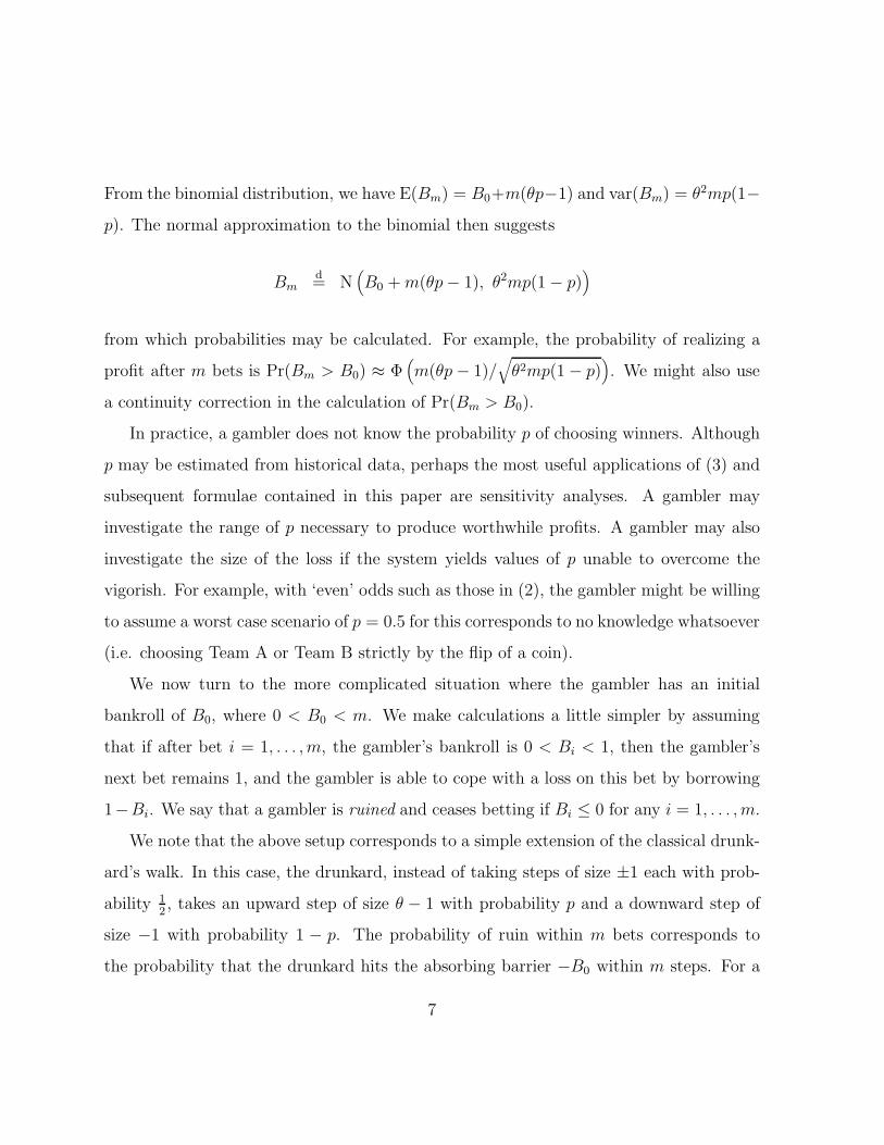
From the binomial distribution, we have E(Bm) = B0+m(θp−1) and var(Bm) = θ2mp(1−

p). The normal approximation to the binomial then suggests

Bmd= N

(

B0 + m(θp − 1), θ2mp(1 − p))

from which probabilities may be calculated. For example, the probability of realizing a

profit after m bets is Pr(Bm > B0) ≈ Φ(

m(θp − 1)/√

θ2mp(1 − p))

. We might also use

a continuity correction in the calculation of Pr(Bm > B0).

In practice, a gambler does not know the probability p of choosing winners. Although

p may be estimated from historical data, perhaps the most useful applications of (3) and

subsequent formulae contained in this paper are sensitivity analyses. A gambler may

investigate the range of p necessary to produce worthwhile profits. A gambler may also

investigate the size of the loss if the system yields values of p unable to overcome the

vigorish. For example, with ‘even’ odds such as those in (2), the gambler might be willing

to assume a worst case scenario of p = 0.5 for this corresponds to no knowledge whatsoever

(i.e. choosing Team A or Team B strictly by the flip of a coin).

We now turn to the more complicated situation where the gambler has an initial

bankroll of B0, where 0 < B0 < m. We make calculations a little simpler by assuming

that if after bet i = 1, . . . , m, the gambler’s bankroll is 0 < Bi < 1, then the gambler’s

next bet remains 1, and the gambler is able to cope with a loss on this bet by borrowing

1−Bi. We say that a gambler is ruined and ceases betting if Bi ≤ 0 for any i = 1, . . . , m.

We note that the above setup corresponds to a simple extension of the classical drunk-

ard’s walk. In this case, the drunkard, instead of taking steps of size ±1 each with prob-

ability 12, takes an upward step of size θ − 1 with probability p and a downward step of

size −1 with probability 1 − p. The probability of ruin within m bets corresponds to

the probability that the drunkard hits the absorbing barrier −B0 within m steps. For a

7

discussion of more general versions of the drunkard’s walk, see Feller (1968, sect. 14.8).

For this problem, the distribution of the final bankroll Bm is expressable via a recur-

sion. For i = 1, . . . , m and j = 0, . . . , i, we define

Qj,i−j = Pr (Bi = B0 + j(θ − 1) − (i − j))

= Pr (j upward steps, (i − j) downward steps, no ruin)

=

pQj−1,i−j + (1 − p)Qj,i−j−1 j > i−B0

θ

0 j ≤ i−B0

θ

where Q0,0 = 1 and Q−1,k = Qk,−1 = 0 for all k. This forms a tree structure where Qj,i−j

is the jth entry along the ith row from the top of the tree. In this case, we construct

the tree beginning with the top element Q0,0 and work downward along rows where the

last row Qj,m−j : j = 0, . . . , m gives the probabilities of interest. We note that the

probability of ruin is available from the final row via Pr(ruin) = 1 −∑m

j=0 Qj,m−j.

Whereas much of the early work corresponding to the drunkard’s walk concerned

itself with approximate solutions and detailed mathematics, we note that the approach

described here is based on ready access to a computing environment; the computational

approach is fast and involves straightforward programming. For example, with θ = 1.91,

B0 = 5, p = 0.56 and m = 500, we obtain Pr(ruin) = 0.428 and this was obtained nearly

instantaneously running Fortran on a SUN workstation.

4. Fixed percentage wagers

In simple fixed percentage wagering, a gambler bets a fraction 0 ≤ f ≤ 1 of the

bankroll on the outcome of a single match. When the outcome of the match is determined,

the gambler resumes fixed percentage wagering on the new balance. Assuming the infinite

divisibility of money, one of the immediate attractions of fixed percentage wagering is that

8

the gambler never goes into debt.

In the context of information theory, Kelly (1956) provided a neat result that is often

quoted but misused in gambling circles. Given a gambling system with probability 0 <

p ≤ 1 of choosing winners and European odds θ > 1, Kelly showed that the ‘optimal’

betting fraction is

f ∗ =pθ − 1

θ − 1(4)

provided that p > 1/θ. For example, consider a system that historically picks winners 54%

of the time (i.e. p = 0.54) with the standard European odds payout of θ = 1.91. In this

case, the optimal betting fraction is 3.45% of the bankroll. The Kelly criteria is optimal

from several points of view; for example, it maximizes the exponential rate of growth and

it provides the minimal expected time to reach a preassigned balance (Breiman, 1961).

Breiman (1961) investigated the properties of betting systems and considered a more

general wagering scenario than the simple situation discussed above. However, Breiman’s

work did not provide the derivation of solutions nor sharp statements concerning the

uniqueness of solutions under the general framework.

We are concerned with restricted problems that are of real interest to the sports bettor.

For example, it is likely that a sports bettor would like to bet on several matches in a

single day. If the bettor uses the Kelly fraction (4) on n such matches where nf ∗ > 1,

then the total amount to bet would exceed the current bankroll. The problem then is to

determine fixed percentages that satisfy some optimality.

We therefore consider the situation where on day j = 1, . . . , m, the gambler wishes to

place nji wagers on matches with European odds θi and where the probability of picking

winners is pi, i = 1, . . . , k. For example, it is possible that a gambler has a system for

betting the pointspread and another system for betting totals (i.e. k = 2). The question

9

arises as to what are the optimal betting fractions f ∗

j1, . . . , f∗

jk on day j where nji wagers

are placed with a fraction fji of the bankroll, i = 1, . . . k? Given an initial bankroll B0,

the bankroll at the completion of day j is

Bj =nj1∏

xj1=0

· · ·njk∏

xjk=0

(

(1 −k∑

i=1

njifji)Bj−1 +k∑

i=1

xjiθifjiBj−1

)∆ji

(5)

where ∆ji = I(Xji = xji), i = 1, . . . , k, in which the random variable Xji denotes the

number of winning wagers of type i on day j. Therefore, only one term in the product

(5) is not equal to 1. Note also that the first term in the outer parentheses is the balance

of the bankroll not bet in a given day and we require∑k

i=1 njifji < 1 to prevent the

possibility of bankruptcy.

Assuming that Xj1, . . . , Xjk are independent with Xji ∼ Bi(nji, pi), i = 1, . . . , k, we are

concerned with the maximization of the function G = G(fj1, . . . , fjk) = E (log(Bj/Bj−1))

where G is referred to as the exponential rate of growth (Breiman, 1961) and

G = E

nj1∑

xj1=0

· · ·njk∑

xjk=0

∆ji log

(

1 −k∑

i=1

njifji +k∑

i=1

xjiθifji

)

=nj1∑

xj1=0

· · ·njk∑

xjk=0

(

k∏

i=1

(

njixji

)

pxji

i (1 − pi)nji−xji

)

log

(

1 +k∑

i=1

fji(xjiθi − nji)

)

. (6)

In the Appendix, we establish the existence of a unique maximum f∗ = (f ∗

j1, . . . , f∗

jk)

and provide a simple algorithm that evaluates f∗. For example, consider a betting system

where k = 3, nj1 = 2, nj2 = 3, nj3 = 3, p1 = 0.545, p2 = 0.565, p3 = 0.585 and

θ1 = θ2 = θ3 = 1.91. The algorithm gives f ∗

j1 = 0.0416, f ∗

j2 = 0.0811 and f ∗

j3 = 0.1215.

The proposed algorithm has worked well in all of the examples that we have considered.

We note however that convergence difficulties were experienced with more sophisticated

10

algorithms taken from numerical libraries. This is due to the fact that in many practical

situations, the function G is nearly flat in neighbourhoods of f∗. As a result, successive

values f (1), f (2), . . . based on derivatives or finite difference methods may oscillate around

the maximum. For example, the IMSL routine duminf based on a quasi-Newton method

failed to converge for the problem described above. The lesson, as always, is that it is

sensible to use available information (e.g. the shape of G) in optimization problems.

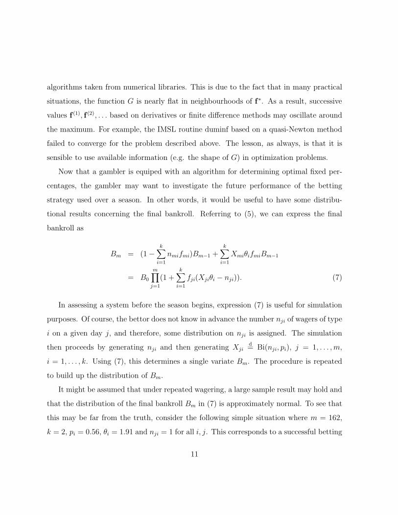
Now that a gambler is equiped with an algorithm for determining optimal fixed per-

centages, the gambler may want to investigate the future performance of the betting

strategy used over a season. In other words, it would be useful to have some distribu-

tional results concerning the final bankroll. Referring to (5), we can express the final

bankroll as

Bm = (1 −k∑

i=1

nmifmi)Bm−1 +k∑

i=1

XmiθifmiBm−1

= B0

m∏

j=1

(1 +k∑

i=1

fji(Xjiθi − nji)). (7)

In assessing a system before the season begins, expression (7) is useful for simulation

purposes. Of course, the bettor does not know in advance the number nji of wagers of type

i on a given day j, and therefore, some distribution on nji is assigned. The simulation

then proceeds by generating nji and then generating Xjid= Bi(nji, pi), j = 1, . . . , m,

i = 1, . . . , k. Using (7), this determines a single variate Bm. The procedure is repeated

to build up the distribution of Bm.

It might be assumed that under repeated wagering, a large sample result may hold and

that the distribution of the final bankroll Bm in (7) is approximately normal. To see that

this may be far from the truth, consider the following simple situation where m = 162,

k = 2, pi = 0.56, θi = 1.91 and nji = 1 for all i, j. This corresponds to a successful betting

11

system for the 2000/2001 National Basketball Association season where the bettor places

a single wager on each of two types of bets every day of the season. The optimal Kelly

fraction (4) is f ∗

ji = 0.0761. Using the simulation procedure based on 1000 simulations,

Figure 1 provides a histogram of the final bankroll B162 using an initial bankroll B0 = 100.

Figure 1 suggests that at the end of the season, the proposed system will probably yield

a small profit (i.e. a final bankroll of less than 1000) although the possibility does exist

for huge profits. We also observe that the final bankroll has a distinctly non-normal

distribution with a very long right tail. However, it is clear that log Bm is a sum of

random variables. Therefore the Central Limit Theorem suggests that log Bm may be

approximately normal. Using the same example as above, Figure 2 provides a histogram

of log B162. The histogram appears more normal and the log data passes the Anderson-

Darling goodness-of-fit test for normality yielding a P -value exceeding 0.5.

We can evaluate the mean E(Bm) using the formula involving conditional expectations:

E(Bm) = B0

(

1 +k∑

i=1

E(njifji)(piθi − 1)

)m

(8)

where it is assumed that the expectation (8) does not depend on the day j.

12

5. Is a gambling system profitable?

Our focus now turns to another practical question: is a proposed gambling system

profitable? Typically, a thoughtful sports bettor, would like to test a gambling system

using historical data before risking his own money. Mok (2001) considers this problem in

more detail than presented here. Consider then a match with European odds

Team A θA (9)

Team B θB

where without loss of generality, we ignore the pointspread. If pA is the true probability

that Team A wins and pB = 1 − pA is the true probability that Team B wins (ignoring

ties), then we should bet on Team A if the expected profit from betting on Team A is

positive. In other words, we should bet on Team A if

(θA − 1)pA + (−1)(1 − pA) > 0 → pA > 1/θA.

Similarly, we should bet on Team B if pB > 1/θB. Recall that pA and pB are unknown

and the inequality 1/θA + 1/θB > 1 is due to the vigorish.

Now we first test the profitability of a gambling system in a restricted context. Suppose

that we have the results of n historical matches where the proposed gambling system would

have bet on Team A with European odds as in (9). Suppose further that x of the n bets

are winning bets. Then we test for a profitable system by considering H0 : pA ≤ 1/θA

versus H1 : pA > 1/θA. The corresponding P -value is given by the binomial probability

Pr(X ≥ x) =n∑

i=x

(ni) (1/θA)i(1 − 1/θA)n−i (10)

13

where a small P -value indicates evidence of a profitable system. This is a simple procedure

to determine whether historical data provides evidence of long-term profitability. For

example, if there are x = 60 winning wagers out of n = 100 matches with standard payout

θA = 1.91, then pA = 1/θA = 0.524 and we have mild evidence (P = 0.076) of a profitable

system. Remarkably, tests such as these are rarely (perhaps never) discussed in the myriad

of gambling books available at the Gamblers Book Shop (www.gamblersbook.com), a key

source for information on gambling.

The situation becomes more complex when bets are placed at various odds. We

have collected data arising from the 2000 Major League Baseball season for which a

proposed betting system was established. Ignoring some of the details, personal odds

were constructed corresponding to Team A defeating Team B. These odds were based on

logistic regression using the pitchers’ earned run averages, overall team batting averages

and team winning percentages as covariates. When the personal odds differed from the

posted odds at the Intertops website (www.intertops.com) by more than 10%, this signaled

a condition to wager.

Table 1 gives the data and P -values for groups of bets placed at 24 differents sets of

odds. The P -values are obtained using (10). We observe that only one of the results are

significant. The problem now is to determine whether the overall system is profitable.

A standard approach is based on Fisher’s test (D’Agostino & Stephens, 1986 p. 357).

Following the notation above, let H0k (H1k) denote the hypothesis that the kth type of

bet is unprofitable (profitable) and let qk denote the corresponding P -value, k = 1, . . . , 24.

Fisher’s test considers the overall null hypothesis Ω0 =⋂24

k=1 H0k versus the alternative

hypothesis that at least one of the H0k is false. Applying Fisher’s test to the data in Table

1, we obtain the overall P -value Pr(χ248 > −2

∑24k=1 log qk) = Pr(χ2

48 > 52.767) = 0.295

which does not allow us to reject the overall null hypothesis Ω0 that all of the component

14

types of bets are unprofitable.

The approach above is not quite right. With respect to the data in Table 1, there is not

enough evidence to reject Ω0, and even if there was, this does not imply that the gambling

system is profitable. We define a profitable gambling system as one for which all of the

H1k are true. Therefore we should instead test Ω0 versus the alternative Ω1 =⋂24

k=1 H1k

and exclude regions of the parameter space that do not belong in Ω0 ∪ Ω1. We exclude

such regions because the gambling system uses the same betting criteria regardless of the

odds and it is therefore logical that if it is an unprofitable (profitable) gambling system,

then it should be an unprofitable (profitable) system for all component types of bets. We

emphasize that the relevant problem is to test a hypothesis Ω0 which is a small set where

all component bets are unprofitable versus a hypothesis Ω1 which is a small set where all

component bets are profitable.

To test Ω0 versus Ω1 in a classical framework, it is natural to reject Ω0 based on large

values of the generalized likelihood ratio statistic

Λ =supΩ0∪Ω1

L(x)

supΩ0L(x)

where L(x) is the corresponding product probability mass function based on the data x.

The exact discrete distribution of Λ is beyond reach since the sample space is so large.

Also, we cannot appeal to a large sample χ2 distribution for 2 log Λ since dim(Ω0) =

dim(Ω1) which means that we have ‘zero’ degrees of freedom. In addition, the supremums

in Λ occur on the boundaries of the parameter space and this invalidates necessary large

sample assumptions.

We consider now a Bayesian approach to testing Ω0 versus Ω1. The Bayesian model

contains a little more structure due to the necessity of prior distributions. Given the

European odds (9), we assume that over many matches the odds are set such that bets

15

Table 1: Betting results using a proposed gambling system; θA is the posted odds forTeam A, θB is the posted odds for Team B, x is the number of wins by betting on TeamA and n is the total number of corresponding matches. The P -value is given and anasterisk indicates significance at level 0.05.

θA θB x n P -value

2.800 1.455 12 32 0.4822.700 1.498 11 25 0.2992.650 1.541 10 23 0.3572.600 1.556 8 18 0.3842.550 1.571 13 34 0.6102.500 1.588 17 35 0.1932.450 1.606 13 38 0.8402.400 1.625 44 89 0.0842.350 1.645 19 43 0.4722.300 1.666 26 56 0.3762.250 1.690 28 59 0.3672.200 1.714 39 65 0.013∗

2.150 1.740 22 43 0.3222.100 1.770 23 41 0.1762.050 1.800 26 47 0.2262.000 1.833 20 39 0.5001.910 1.910 9 17 0.5781.833 2.000 12 20 0.3991.800 2.050 4 7 0.6201.770 2.100 29 51 0.5381.740 2.150 4 6 0.4921.690 2.250 3 3 0.2071.645 2.350 3 5 0.6961.625 2.400 3 5 0.709

16

on Team A and Team B are equally attractive (i.e. they yield the same expected return).

Therefore, based on a unit bet,

(θA − 1)pA + (−1)(1 − pA) = (θB − 1)(1 − pA) + (−1)pA → pA = θB/(θA + θB)

where θB/(θA + θB) represents the expected probability that Team A wins and the expec-

tation is taken over many matches. In any particular match, the true probability pA may

be something different than θB/(θA + θB). Let Xk denote the number of winning bets of

type k out of nk wagers and let p(0)k = θB/(θA + θB) for the kth type of bet, k = 1, . . . , N .

For the data in Table 1, N = 24. This suggests the hierarchical model

(Xk | pk)d= Bi(nk, pk) k = 1, . . . , N

(pk | m)d= β

(

mp(0)k , m(1 − p

(0)k )

)

k = 1, . . . , N

md= U(l,∞) where l = maxk

(

1/p(0)k , 1/(1 − p

(0)k )

)

(11)

where the pk are conditionally independent. The beta prior for pk is reasonable from the

point of view that pk is constrained to the interval (0, 1) and E(pk | m) = p(0)k as argued

previously. The hyperparameter m controls the variance of the pk, and we assign a flat

improper prior for m. We include the lower limit on m as this forces concave densities for

p1, . . . , pN .

The hierarchical model (11) induces a (N +1) dimensional posterior distribution given

by (p, m | x). Inference based on (p, m | x) is straightforward using the Gibbs sampling

algorithm as the full conditional distributions of the pk are beta distributions and m

can be generated in closed form from its full conditional distribution via inversion. To

obtain the posterior probabilities of Ω0 and Ω1, we simply calculate the proportion of the

generated ps that fall into the two respective sets. For the data in Table 1, it turns out

17

that both of these probabilities are essentially zero.

We are therefore faced with the problem of assessing two hypotheses Ω0 and Ω1, one

of which we believe to be true, when both hypotheses correspond to very improbable sets.

This is a general problem of inference which goes beyond the application considered here.

Our approach which borrows on ideas from Swartz (1999) and Evans et al. (1997) is to

generate p from the Gibbs sampling algorithm and then calculate its Euclidean distance

D0 from Ω0 and its Euclidean distance D1 from Ω1. The smaller (larger) the quantity

D0/D1, the more evidence p provides in favour of the hypothesis Ω0 (Ω1). We therefore

consider posterior probabilities Pr(D0/D1 ≤ t | x) for different values of t. To put more

reliance on the data we also calculate the Bayes factor

BFD =Pr(D0/D1 ≤ t | x)

Pr(D0/D1 > t | x)

Pr(D0/D1 > t)

Pr(D0/D1 ≤ t)

where small (large) values give evidence in favour of Ω1 (Ω0). There is one difficulty with

the calculation of BFD and this concerns the improper prior for m. With an improper

prior, we are unable to generate from the joint prior distribution of (p, m) to obtain

Pr(D0/D1 ≤ t) and Pr(D0/D1 > t). For the data in Table 1, we therefore set m = 2.98

which is the posterior mean of m estimated from the output of the Gibbs sampling algo-

rithm, and we then simulate the pks from the beta priors with this value of m. Table 2

shows BFD, the posterior odds of D0/D1 ≤ t and the prior odds of D0/D1 ≤ t correspond-

ing to the data in Table 1. As expected, we see that both the posterior odds and prior

odds are increasing in t. However, the prior odds are larger and increase more rapidly

than the posterior odds. This causes the Bayes factor BFD to be small and approach zero

as t increases. We also observe that BFD has its largest value when t is around 1.

Now if you have confidence that the prior is realistic, then it is often argued that

inference should be based solely on the posterior as Bayes Theorem provides the recipe

18

Table 2: BFD, the posterior odds of D0/D1 ≤ t, the prior odds of D0/D1 ≤ t for selectedvalues of t using the data in Table 1.

t BFD posterior odds prior odds

0.6 0.009 0.001 0.1140.7 0.030 0.008 0.2710.8 0.035 0.018 0.5220.9 0.046 0.040 0.8591.0 0.051 0.081 1.5911.2 0.048 0.203 4.2081.4 0.036 0.410 11.5001.6 0.025 0.631 25.3161.8 0.014 0.996 70.4292.0 0.012 1.532 124.0002.5 0.006 3.219 499.0003.0 0.000 5.410 ∞4.0 0.000 13.925 ∞6.0 0.000 70.429 ∞8.0 0.000 165.667 ∞

19

for combining information from the data (i.e. the likelihood) and information from the

prior. In this case, the posterior odds from Table 2 clearly suggest that the gambling

system is profitable based on the data in Table 1. Note that using the posterior odds for

t = 1.0 in Table 2, we obtain Pr(D0 < D1 | x) = 0.075.

Now if you have less faith in your prior, then you may want to base your inference

on the Bayes factor as it relies more strongly on the data by factoring out the prior

odds. Since the Bayes factor BFD is very small for different values of t in Table 2, this

gives strong evidence in favour of Ω1 under the assumption that Ω0 and Ω1 are the only

possibilities in the parameter space. For example, observe that the Bayes factor is roughly

at least 20 times more favourably inclined toward Ω1 than Ω0. Therefore, in contrast to

the previous analyses, the Bayesian analyses using both posterior probabilities and Bayes

factors suggest that the data in Table 1 provide evidence of a profitable system.

The underlying practical problem has lead to a significant theoretical problem involv-

ing the testing of non-standard hypotheses.

6. Discussion

Now suppose that you have a ‘winning’ system. How should you bet? Typically,

Sportsbooks assign an upper limit on wagering. Since the Kelly approach has an optimal

rate of growth, it seems logical to begin with the Kelly system using fixed percentage

wagering until the upper limit is attained. As long as the Kelly system prescribes a bet

exceeding the upper limit, use fixed wagering with the upper limit.

Sportsbooks also typically assign a lower limit on wagering. For some internet sites,

the lower limit is so low (e.g. $1 at www.intertops.com) that it can be practically ignored.

We recommend an alternative betting strategy that also allows us to ignore the lower

limit on wagering. Suppose that you have an initial bankroll B0 = $500 and that you are

20

wagering at a Sportsbook with a lower limit of $10 and an upper limit of $3000. Extensive

personal simulations have shown that it is better to begin with the Kelly system using

a bankroll of x1 = $400, and if the bankroll drops below x2 = $200, add the final $100

to the bankroll. The idea is to ‘kickstart’ the system since a very small bankroll grows

slowly with fixed percentage wagering. It would be interesting to see if optimal values for

x1 and x2 could be obtained. Again, as long as the prescribed value of Kelly wagering

exceeds $3000, you would maintain $3000 betting.

The results that we have presented in this paper are readily applicable to sports

betting. The real difficulty is coming up with a winning system (i.e. a system where

p is sufficiently large to overcome the vigorish). Naturally p is unknown, and therefore

we might estimate p for a proposed system using past data. Of course, there is no

guarantee that results will replicate from year to year, and we need also be wary of

multiple comparisons issues when considering various systems.

Appendix: the maximization of G

In the context of simultaneous fixed percentage wagers, we consider the maximization

of the function G in (6). The first and second derivatives of G are given by

Gi =∂G

∂fji

=nj1∑

xj1=0

· · ·njk∑

xjk=0

(

k∏

i=1

(

njixji

)

pxji

i (1 − pi)nji−xji

)

xjiθi − nji

1 +∑k

i=1 fji(xjiθi − nji)

and

Gi1i2 =∂2G

∂fji1∂fji2

=nj1∑

xj1=0

· · ·njk∑

xjk=0

(

k∏

i=1

(

njixji

)

pxji

i (1 − pi)nji−xji

)

−(xji1θi1 − nji1)(xji2θi2 − nji2)

(1 +∑k

i=1 fji(xjiθi − nji))2

for i, i1, i2 = 1, . . . , k. Now G is a continuous function defined on the intersection of [0, 1)k

21

and the halfspace∑k

i=1 njifji < 1. When pi > 1/θi, i = 1, . . . , k, we obtain

(a) Gi > 0 when fji = 0, i = 1, . . . , k,

(b) Gi1i2 < 0 everywhere for i1, i2 = 1, . . . , k

and (c) G → −∞ ask∑

i=1

njifji → 1.

Using these results, and by considering closed sets that approach the region of interest, it

can be shown that there is a single critical point lying in the interior of the region, and

this point is a global maximum. This establishes the uniqueness of f ∗

j1, . . . , f∗

jk. Since

G(0) = 0, we also have that G(f∗) > 0.

The shape and smoothness of G yields a simple algorithm which is guaranteed to find

f ∗

j1, . . . , f∗

jk. We begin by initializing an interior point fji = 1/∑k

i=1 2nji, i = 1, . . . , k. To

obtain the root of G1 along the first coordinate direction, bisection is carried out using the

lower starting value f(l)j1 = 0 and the upper starting value f

(u)j1 which intersects the plane

∑ki=1 njifji = 1. After the first coordinate is updated, the procedure is repeated along the

coordinate directions 2, . . . , k. The loop in this sequential procedure is repeated until the

movement in the point is sufficiently small. The maximum has then been obtained. The

proposed algorithm is a special case of Gauss-Seidel iteration (Thisted 1988, page 187)

where success is based on the recognition that every step of bisection results in a move

up the hill and that there are no saddle points or minima of the function G.

References

Breiman, L. (1961). Optimal gambling systems for favorable games. Proceedings of the Fourth

Berkeley Symposium on Mathematical Statistics and Probability, Jerzy Neyman, editor,

65-78.

Crist, S. (1998). All bets are off. Sports Illustrated, 88 (3), 82-92.

22

D’Agostino, R.B. & Stephens, M.A. (1986). Goodness-of-Fit Techniques, Marcel Dekker, New

York.

Evans, M., Gilula, Z., Guttman, I. & Swartz, T.B. (1997). Bayesian analysis of stochasti-

cally ordered distributions of categorical variables. Journal of the American Statistical

Association, 92, 208-214.

Feller, W. (1968). An Introduction to Probability Theory and its Applications, Volume 1, Third

Edition, John Wiley and Sons, Inc.

Haywood, H. (2000). BeatWebCasinos.Com: The Shrewd Player’s Guide to Internet Gambling,

RGE Publishing, Oakland, California.

Kelly, J.L. (1956). A new interpretation of information rate. Bell System Technical Journal,

35, 917-926.

McCune, B. (1989). Education of a Sports Bettor, McCune Sports Investments, Las Vegas,

Nevada.

Mok, L. (2001). Testing whether a gambling system is profitable. MSc project, Simon Fraser

University, Department of Statistics and Actuarial Science.

Ordine, B. (2000). Super bowl Sunday means lots of action in Las Vegas. Seattle Times,

January 23.

Productivity Commission (1999). Australia’s gambling industries (Report No 10), PC Inquiry

Report, December, www.pc.gov.au/inquiry/gambling/finalreport/index.html.

Stern, H.S. (1998). How accurate are the posted odds?. In the column A Statistician Reads

the Sports Pages, Chance, 10 (4), 17-21.

Swartz, T.B. (1999). Nonparametric goodness-of-fit. Communications in Statistics: Theory

and Methods, 28, 2821-2841.

23

Thisted, R.A. (1988). Elements of Statistical Computing: Numerical Computation, Chapman

and Hall, New York.

Thorp, E.O. (1969). Optimal gambling systems for favorable games. Review of the Interna-

tional Statistical Institute, 37, 273-293.

24

0 2000 4000 6000 8000 10000

020

040

060

0

Figure 1: Histogram of the final bankroll based on 1000 simulations

final bankroll

freq

uenc

y

25

2 4 6 8

020

4060

Figure 2: Histogram of the logarithm of thefinal bankroll based on 1000 simulations

log(final bankroll)

freq

uenc

y

26