IYPT 2010 Austria, I. R. Iran Reporter: Reza M. Namin 1

IYPT 2010 Austria, I. R. IranIYPT 2010 Austria, I. R. Iran

Problem No.

1

ROTATING SPRING

Reporter: Reza M. Namin

16

IYPT 2010 Austria, I. R. Iran2

The problem• A helical spring is rotated about one of its ends around

a vertical axis.

• Investigate the expansion of the spring with and without an additional mass attached to it’s free end.


Main approach• Theory

– Background– Theory base– Developing the equations– Numerical solution

• Experiment– Setup– Parameters, results and comparison

• Conclusion


Theory - Background

• Act of a spring due to tensile force:– Hook's law: F = k ∆L

• F: Force parallel to the spring• k: Spring constant• ∆L: Change of length

– A spring divided to n parts:• F = n k ∆L• μ = k L remains constant

• Circular motion– a = r ω2

• a: Acceleration• r: Distance from the rotating axis• ω: Angular velocity


Theory - Base

• Effective parameters:– ω: Angular velocity– λ : Spring liner density = m / l – M: Additional mass– μ : Spring module = k l– l, l1, l2: Spring geometrical properties

M

l1 l l2


Theory - Base

• Looking for the stable condition in the rotating coordinate system– Accelerated system → figurative force

• Acting forces:– Gravity– Spring tensile force– Centrifugal force


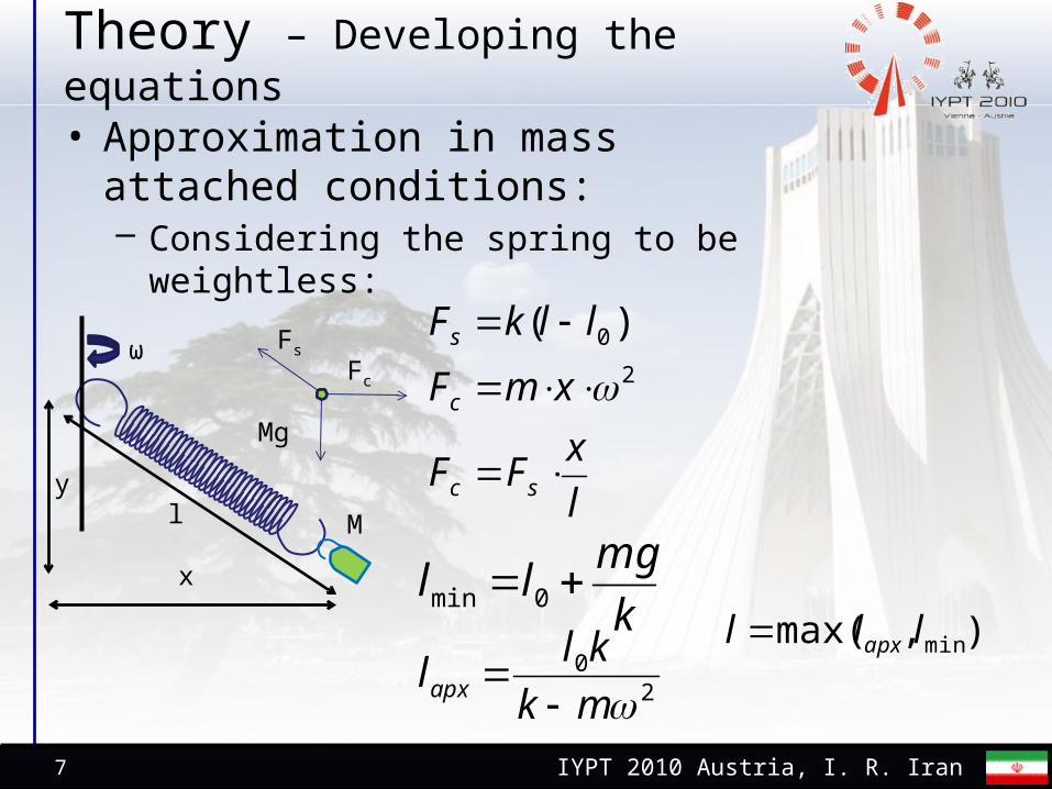
Theory – Developing the equations• Approximation in mass attached

conditions:– Considering the spring to be

weightless:

l M

ω

x

y

Fs

Fc

Mg

l

xFF

xmF

llkF

sc

c

s

2

0 )(

20

mk

kllapx

k

mgll 0min

),max( minlll apx


Theory – Developing the equations• Exact theoretical description:

– Problem: The tension is not even all over the spring…

– Solution: Considering the spring to be consisted of several small springs.

M


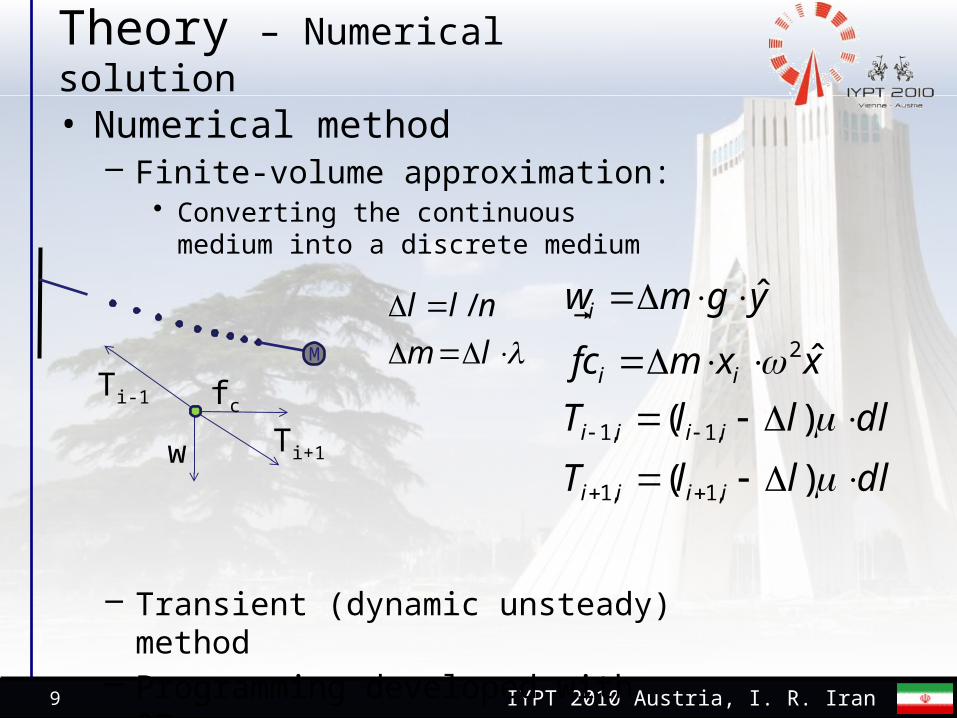
Theory – Numerical solution

• Numerical method– Finite-volume approximation:

• Converting the continuous medium into a discrete medium

– Transient (dynamic unsteady) method– Programming developed with QB.

M

dlllT

dlllT

xxmcf

ygmw

iiii

iiii

ii

i

)(

)(

ˆ

ˆ

,1,1

,1,1

2

w

Ti-1

Ti+1

fc

lm

nll /



Mesh independency check

80 85 90 95 100 105 110 115 1200.15

0.2

0.25

0.3

0.35

0.4

0.45

n = 5

n = 10

n = 15

Angular velocity (s-1)

Sp

rin

g le

ngt

h (

m)

n: Number of mesh points

As n increases, the result will approach to the correct answer



Tension in different points of the spring with different additional mass amounts:

0 2 4 6 8 10 12 14 16 180

0.2

0.4

0.6

0.8

1

1.2

1.4

m = 0m = 2.5gm = 5g

Position in the spring (cm)

Ten

sion

(N

)


Experiment• Finding spring properties

– Direct measurement: Mass & lengths– Suspending weights with the spring to

measure k and μ

• Changing the angular velocity, measuring the expansion– Change of the angular velocity with different

voltages– Measuring the angular velocity with

Tachometer– Measuring the length of the rotating spring

using a high exposure time photo


Experiment setup

The motor, connection to the spring and the sensor sticker


Experiment setup

The rotating spring and tachometer


Experiment setup

Hold and base


Experiment setup

All we had on the table


Experiments

Suspending weights with the spring

Finding k and using that to find μ

0.05 0.06 0.07 0.08 0.09 0.1 0.11 0.120

0.5

1

1.5

2

2.5

f(x) = 33.782655313683 x − 1.84774791757864R² = 0.999226158045033

Spring length (m)

Att

ache

d w

eigh

t (N

)

→K = 33.78 N/m

→μ = K l = 1.824 N


Experiments

Expansion increases with increasing angular velocity


Experiments

Measurement of length in different angular velocities

Comparison with the numerical theory

10 20 30 40 50 60 70 80 900

5

10

15

20

25

ExperimentsNumerical result

Angular velocity (Rad / s)

Spri

ng le

ngth

(cm

)

λ =0.148 kg/mμ =1.824 Nl1 =1.5 cml2 = 1.7 cm


Experiments

Comparing the shape of the rotating spring in theory and experiment

0.0000 0.0500 0.1000 0.1500 0.2000 0.2500 0.3000

-0.1000

-0.0900

-0.0800

-0.0700

-0.0600

-0.0500

-0.0400

-0.0300

-0.0200

-0.0100

0.0000

λ =0.103 kg/mμ =0.369 Nl = 16.3 cml1 =1 cmω = 120 RPM


Experiments

Investigation of the l-ω plot within different initial lengths

100 150 200 250 300 3500

5

10

15

20

25

30

35

40

45Experiment: l = 16.3Experiment: l = 14Experiment: l = 11.5Experiment: l = 7.2Numerical: l = 16.3Numerical: l = 14Numerical: l = 11.5Numerical: l = 7.2

Angular velocity (RPM)

Sp

rin

g le

ngt

h (

cm)

λ =0.103 kg/mμ =0.369 Nl1 =1 cm


Experiments

Comparison between the physical experiments, numerical results and theoretical approximation within different additional masses

0 50 100 150 200 250 300 350 400 4500

5

10

15

20

25

30

35

40

45Exp M = 0

Exp M = 5g

Exp M = 10g

Exp M = 15g

Num M = 0

Num M = 5g

Num M = 10g

Num M = 15g

Appx M = 0

Appx M = 5g

Appx M = 10g

Appx M = 15g


Sp

rin

g le

ngt

h (

cm)

λ =0.103 kg/mμ =0.369 Nl = 5.4cml1 =1 cm


Conclusion• According to the comparison

between the theories and experiments we can conclude:– In case of weightless spring

approximation:

20

mk

kllapx

k

mgll 0min

),max( minlll apx


Conclusion

• In general, the numerical method may be used to achieve precise description and evaluation.

• Some of the results of the numerical method are as follows:


Conclusion

Numerical solution results

Change of the spring hardness

0 50 100 150 200 250 300

-0.0999999999999994

5.82867087928207E-16

0.100000000000001

0.200000000000001

0.300000000000001

0.400000000000001

0.500000000000001

0.600000000000001miu = 0.1

miu = 0.2

miu = 0.3

miu = 0.5


Sp

rin

g le

ng

th (

m)

λ =0.1 Nl = 10 cml1 =1 cm

IYPT 2010 Austria, I. R. Iran

0 50 100 150 200 250 300 3500

0.05

0.1

0.15

0.2

0.25

0.3

0.35

0.4

0.45

0.5

Landa = 0.05

Landa = 0.1

Landa = 0.15

Landa = 0.2

Conclusion


Change of spring density

μ =0.3 Nl = 10 cml1 =1 cm


0 50 100 150 200 2500

0.05

0.1

0.15

0.2

0.25

0.3

0.35

0.4

l = 8cm

l = 10cm

l = 12cm

l = 14cm


Sp

rin

g len

gth

(m

)Conclusion

Numerical solution result

Change of initial length

λ =0.2 kg/mμ =0.3 Nl1 =1 cm


Conclusion


Change in additional mass

0 20 40 60 80 100 120 140 160 1800

0.05

0.1

0.15

0.2

0.25

0.3

0.35

0.4

0.45

0.5m = 0

m = 5g

m = 10g

m = 15g


Sp

rin

g len

gth

(m

)

λ =0.2 kg/mμ =0.3 Nl = 10cml1 =1 cm

IYPT 2010 Austria, I. R. IranIYPT 2010 Austria, National team of I. R. Iran

Thank you

Documents

IYPT 2010 Austria, I. R. Iran Reporter: Reza M. Namin 1