Embed Size (px)
Citation preview
AN ABSTRACT OF THE THESIS OF
Ron R. Meyersick for the degree of Master of Science
in Agricultural and Resource Economics presented on
September 16, 1987
Title: Assessment of Alternative Raw Product Valuation
Methodology With Respect To Cooperatives Single
Pool Returns
Abstract approved:
^J James C. Cornelius
The market for Oregon's processing vegetables has un-
dergone extensive structural changes in recent years. The
role of the cash market between grower and processor has
declined in importance, as proprietary processors have
relocated outside the Willamette Valley, or been forced
out of business entirely. This places increased pressure
on producer-owned cooperative processors to synthesize the
forces of supply and demand for the raw product.
Synthesizing raw product prices in a vertically in-
tegrated structure creates the possibility of inefficient
price signals. Prices set too high or too low at the raw
product level may lead to raisallocated contracted acreage
and inappropriate production levels in relation to
finished product market conditions. Furthermore, raw
product price is used as a basis for calculating payments
to growers under the single pool accounting framework used
by many cooperatives. In a single pool, all commodities
are included together by the cooperative in a single
account; revenues from sale of all the processed products
are added together and total processing costs are sub-
tracted to arrive at the pool's net revenue. The frac-
tional shares of net revenues payable to individual
growers are then based upon the cooperative's estimate of
per unit raw product values. Thus, raw product value es-
timates that are too low or too high will lead to misal-
location of returns to individual members. The objective
of the present research is to develop alternative raw
product valuation procedures, and to assess the perfor-
mance of these procedures in allocating member returns in
single-pool cooperative. A raw product's value is taken
to be the forecasted net return of processing and selling
that product.
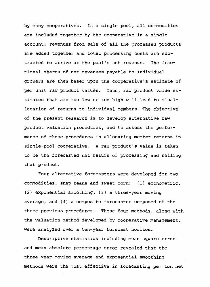
Four alternative forecasters were developed for two
commodities, snap beans and sweet corn: (1) econometric,
(2) exponential smoothing, (3) a three-year moving
average, and (4) a composite forecaster composed of the
three previous procedures. These four methods, along with
the valuation method developed by cooperative management,
were analyzed over a ten-year forecast horizon.
Descriptive statistics including mean square error
and mean absolute percentage error revealed that the
three-year moving average and exponential smoothing
methods were the most effective in forecasting per ton net
returns. When used to set "economic values" of raw
products, these methods also were the most effective in
equating expected member pool payments with expected net
returns. However, the cooperative's present method of es-
tablishing "economic values" for raw products produced the
smallest variance in the difference between pool payments
and net returns.
Assessment of Alternative Raw Product Valuation Methodology With Respect to
Cooperatives Single Pool Returns
by
Ron R. Meyersick
A THESIS
presented to
Oregon State University
in partial fulfillment of the requirements for the
degree of
Master of Science
Completed September 16, 1987
Commencement June 1988

APPROVED:
Asspciaue Professor of Agricultural and Resource ^Economics in charge of major
Head, Agricultural and Resource Economics
tr Dean of Graduate School
Date thesis presented September 16, 1987
Typed by Dodi Reesman for Ron R. Meyersick

ACKNOWLEDGMENTS
Special gratitude and appreciation is expressed to
Dr. James Cornelius for making this research project pos-
sible. Dr. Cornelius must be thanked specifically for
many things. Above all, thanks must be expressed for Dr.
Cornelius' generosity with time and never-ending patience,
also for the ability to keep the essentials of this re-
search project in perspective and finally the unlimited
discussions of anadromous creatures and birds of flight to
ease times of anxiety during critical stages of this
project.
A special thank you to Dr. Steven Buccola for many
useful suggestions. Dr. Buccola's willingness to help and
sense of direction gave this research essential guidance
in many critical areas. Without guidance from Dr. Buccola
this paper may never have been completed.
A very special thanks to my parents for their endless
support. The always present encouragement they have given
me, in large part, has been responsible for an excellent
education.
A thank you is also extended to Dodi Reesman for her
sense of humor and valuable help in typing this paper as
time ran short.
TABLE OF CONTENTS
Chapter Page
I Introduction 1
Situation 1
Problem 1
Ob j ectives 4
Procedures 5
Limitations 6
Thesis Organization 6
II Conceptual Model 8
Market Pools 8
Member Payment Calculations 10
Price Determination 13
Raw Product Market 14
Processed Vegetable Market 15
Forecasting Raw Product Prices 16
Econometric Model Conceptualization 21
Econometric Conceptual Model 22
Econometric Relationship 23
Technical Forecasting Method 24
Single Moving Average 28
Composite Forecasting 29
Summary 32
III Model Specification 33
Accounting Period 33
Pool-Year Econometric Model 34
The Dependent Variable 34
TABLE OF CONTENTS (continued)
Chapter Page
The Explanatory Variables 37
Supply 37
Demand 38
Model Formulation 39
Pool Payments 40
Data Sources 42
Dependent Variable 42
Independent Variables 43
Summary 44
IV Results 45
Sample Size and Forecast Interval 45
Model Specification Criterion 46
Forecasting Comparative Statistics 46
Mean Square Error 47
Mean Absolute Percentage Error 47
Parameter Evaluation of Econometric and Exponential Smoothing Models 48
Econometric Model: Snap Beans 48
Interpretation 48
Econometric Model: Sweet Corn 51
Interpretation 53
Exponential Smoothing Results 54
Interpretation 54
Pool Year Returns 56
Evaluation of Forecasting Techniques.... 56
TABLE OF CONTENTS (continued)
Chapter Page
Evaluation Procedure 56
Forecasting Comparative Statistics 58
Graphical Analysis 60
Comparison of Pool-Year Returns 60
Summary 66
V Summary and Conclusions 68
Assessment of Alternative Forecasting Methods With Respect to Pool-Year Returns 68
Forecasting Methods 69
Econometric Models 69
Naive Forecasters 70
Composite Forecaster 71
Applications for Single-Pool Cooperatives 71
Limitations 73
Suggestions for Further Research 74
Bibliography 76
Appendix A: Pool-Year Returns and Comparative Statistics 78
Appendix B: Econometric Model Estimation Results 81
Appendix C: Data for Econometric Model Estimation 90
LIST OF FIGURES
Figure Page
3.1 Time Line Illustrating Pool Year Net Returns Calculation and Forecast Date 35
4.1 Alternative Raw Product Value Forecasts: 1976-1985 (Snap Beans) 61
4.2 Alternative Raw Product Value Forecasts: 1976-1985 (Sweet Corn) 62
LIST OF TABLES
Table Page
2.1 Estimation Results: Selected Tomato Products 18
2.2 Estimation Results: Canned and Frozen Beans and Corn 20
2.3 Smoothing Results Canned and Frozen Beans and Corn 26
2.4 Hog, Cattle and Broiler Forecasts, A Comparison of Alternative Methods 31
4.1 Estimation Results: Snap Beans 49
4.2 Estimation Results: Sweet Corn 52
4.3 Estimation Results: Exponential Smoothing 55
4.4 Pool-Year Calculation and Comparisons Among Alternative Forecasters 57
4.5 Comparative Forecast Statistics 59
ASSESSMENT OF ALTERNATIVE RAW PRODUCT VALUATION
METHODOLOGY WITH RESPECT TO COOPERATIVES
SINGLE POOL RETURNS
CHAPTER I
INTRODUCTION
Situation
The market for Oregon's Willamette Valley processing
vegetables has undergone extensive structural changes in
recent years. The role of the cash market between grower
and processor has declined in importance as proprietary
processors have relocated outside the Willamette Valley or
been forced out of business entirely. Since cash market
prices of raw products traditionally have been used as
part of the formula for determining members' shares of
pool net returns, cooperatives are under increased pres-
sure to find alternative ways of establishing raw market
values.
Problem
There are several interrelated market problems aris-
ing from the restructuring of the Willamette Valley pro-
cessed vegetable industry. Financial and operating records
obtained from a representative agricultural processing and
marketing cooperative provide the basis for illustrating
the nature of the raw product pricing dilemma. The con-
fidential nature of this information precludes the dis-
closure of certain sensitive financial data, and the
anonymity of the firm is maintained throughout this
thesis. The cooperative uses raw product "price" as a
basis for payments to grower-members. As proprietary
private processors have relocated outside the Willamette
Valley, the number of independent market transactions be-
tween grower and the buyer of raw product has been
reduced. Thus, signals other than competitive market
prices are now relied on to generate estimates of raw
product values.
Each year before contracting acreage, cooperative
management forecasts raw product values. These values are
then relied upon by the cooperative in determining the
number of acres to contract out. Grower-members also rely
on these estimated values for production decisions.
Raw product values which are simulated within a ver-
tically integrated structure such as a processing coopera-
tive create the possibility of inefficient prices. Many
cooperative vegetable processors operate on a pool basis,
in which net revenues from all processed products are
pooled together. The fractional shares of net revenue
payable to individual growers are then based on the per-
unit raw product values of each commodity delivered to the
cooperative (Buccola and Subaei, 1985). Thus, inefficient
raw product values will induce misallocation of payments
back to growers. An economic value!/ for an individual
commodity which is too high or too low will result in a
subsidy or tax, respectively, to the grower of that com-
modity in a single pool, assuming the finished products
are sold at competitive equilibrium prices.
This problem is further complicated by the fact that
the cooperative relies upon the estimated price for ob-
taining raw product. Assuming a positive production
response to raw product values, estimated prices set
either too high or too low will result in inappropriate
supply levels relative to the true but unobservable equi-
librium in the processed wholesale market. With raw
product values set above the equilibrium price, an excess
production response from growers will occur. Faced with
increasing competition in the finished product market from
other regions in the U.S., Willamette Valley growers may
find themselves with increased production and excess sup-
plies but a smaller share of the market due to the artifi-
cially high raw product price. Similarly, a raw product
price set to low might divert acreage from a desired
vegetable crop. This may produce lower returns to the
pool of revenues, relative to those which could have been
y Economic value refers to the estimated value of a raw product as determined by cooperative management.
obtained if the increased demand in the finished product
market was accurately reflected in the raw product price.
Raw product pricing in a vertically integrated struc-
ture can create a misallocation of resources at the firm
level (Tomek and Robinson, 1982). Potential solutions to
this valuation problem include the development of alterna-
tive pricing procedures at the raw product level.
Examination of time series data reveals that the raw
product values simulated by the cooperative for selected
vegetables have varied, on average, from the ex post cal-
culated values based on finished product prices less
relevant processing costs. While some variation in es-
timated versus actual value is expected, a long-term
average difference between the two implies per-ton pool
returns are distorted.
The cooperative is currently relying upon a relative
simple estimation procedure stipulated by its by-laws to
generate raw product prices. Other forecasting methods
have been developed and could be used to augment the ex-
isting procedures.
Objectives
The overall objective of this research is to explore
the performance of alternative raw product valuation pro-
cedures for a vertically integrated vegetable processing
and marketing cooperative. This will be accomplished in
two steps. First, alternative raw product forecasting
techniques will be developed and evaluated. Four such al-
ternatives will be utilized to forecast raw product
values. Second, these methods, along with the method cur-
rently employed by the cooperative, will be used to simu-
late single pool returns. This will allow comparisons of
the different forecasting techniques in terms of the
equity of members' associated pool payments.
Procedures
An econometric model, exponential smoothing model,
and a three year moving average model will be used to
forecast values for raw product. The econometric model
will be estimated using ordinary least squares regression
incorporating relevant supply and demand variables. These
methods then will be used collectively to form a composite
fourth forecast for raw product values. Each alternative
forecasting technique can be used to calculate simulated
single pool returns along with the methodology now
employed by the cooperative. These four simulated pool
returns, along with the valuation procedure used by the
cooperative, will then be compared to the actual net
returns to assess the accuracy and suitability of alterna-
tive methods.
Limitations
The cooperative upon which this research is based
handles nine principal fruit and vegetable products. Cur-
rently these products are all accounted for within a
single pool framework.1/ This research utilizes the same
pool calculation method for establishing pool returns as
does cooperative management. That is, payments to grower-
members are calculated from a single pool of revenues.
However, this paper only includes two commodities, while
the cooperative handles nine separate conunodities within a
single pool. In this sense, the pool results developed in
this paper are simulated and not directly representative
of the nine-commodity single pool operated by cooperative
management.
Thesis Organization
Chapter II describes relevant market mechanisms upon
which this research is based, and the rationale for
forecasting raw product values. Previous research in this
area is cited and the conceptual framework for the alter-
native valuation procedures is discussed.
The accounting procedure used by cooperative manage-
ment is given in Chapter III. Following the development
of the time setting for raw product forecasts, the pool-
i.' Discussed in Chapter II, page 9.
year econometric models are given in detail. The chapter-
concludes with a discussion of the methodology used for
the calculation of single-pool payments.
In Chapter IV the model specification criterion will
be outlined along with goodness-of-fit criteria to be used
in evaluation of the alternative forecasting techniques.
Results of all models and subsequent pool payments are
then presented and evaluated.
Results are summarized and limitations associated
with the research are discussed in Chapter V. The chapter
concludes with suggestions for further research.
Appendix A contains estimation results for the
econometric models. Appendix B gives the results for the
pool-year calculations and Appendix C lists the data used
to estimate the econometric models.
CHAPTER II
CONCEPTUAL MODEL
"A cooperative is a private decision-making and risk bearing organization whose equity is held by patrons. Its limits are its physical facilities and its perceived market potentials. The cooperative is a joint vertical expansion, and an integral part of each members opera- tions. Its objectives are to maximize the wel- fare of the members from their own decision management" (Garoyan, 1983).
In an effort to maximize the welfare of grower-
members, it is essential that cooperative management take
into account prices in both the raw and finished product
markets. This chapter presents a discussion of market
pools and grower-member payments based upon single-pool
framework. The relevant market mechanisms are given, with
particular emphasis on the raw product market. An
econometric model will be specified along with a descrip-
tion of other alternatives to the current raw product
valuation forecasting method used by cooperative manage-
ment. A review of literature is included noting previous
research where applicable.
Market Pools
Agricultural processing cooperatives such as Wil-
lamette Valley vegetable processors, which handle a
variety of commodities, must establish a method for al-
location of net revenues to grower-members.
"Most agricultural processing and marketing cooperatives return net revenues to members on a pooling basis. Pooling involves combing the sales revenue, less processing costs of a class of products and allocating these net revenues among members according to a prearranged for- mula. The alternative to pooling is to segregate each members delivers until final sale and to compensate the members exclusively on the basis of the sale of such products. This usually is impractical in large, highly mechanized processing and handling systems" (Buccola and Subaei, 1983).
There is a wide range of pool structure pos-
sibilities. Subaei (1984) noted that the number of pos-
sible pooling rules is equal to the number of all possible
combinations of feasible pool breadths and share valuation
methods. Extensive research was conducted by Subaei to
determine an optimal pool choice among cooperative mem-
bers. Selection criteria used for pool choice were the
risk preference of cooperative members as well as the
schemes used to weight individual choices. The group op-
timal choice usually was to operate separate vegetable
pools and to value raw products on a farm price basis.
On one extreme, a pool may be operated for each in-
dividual commodity handled. The other extreme would be to
group all commodities handled into a single pool.-i.'
1/ In a single pool, all commodities are included together by the cooperative in a single account, and revenues from the sale of all these processed products are added together from which is deducted the total processing costs to arrive at the pools net revenue (Subaei, 1984).
10
Several other possibilities fall in between these two ex-
tremes. Frequently, a single pool is operated due to the
commingling of products such as mixed fruits and
vegetables. In operating this single pool, the board of
directors assigns an established or economic dollar value
per-raw-unit in March of each year for each different
product it handles. The economic value is a forecasted
price upon which growers may base resource allocation
decisions for planting specific vegetable crops. The
economic value paid for raw products would ordinarily be
dependent on prices paid by private processors for the
same commodities in the region where the cooperative
operates (Subaei, 1984). With the disappearance of
private processors in Oregon, this is becoming more dif-
ficult.
Member Payment Calculations
"Pooling involves the consideration of three
practices: (1) The mingling of products of individual
producers into a collective lot; (2) pooling the expenses
of operations and allocating them against products
handled; and (3) prorating sales among producers contribu-
tions to the pool" (Roy, 1976). This last consideration
is often seen as the most important among grower-members.
"Cooperatives are obligated to distribute among mem-
bers any excess of final product sales revenues over
11
operating costs" (Buccola and Subaei, 1985). Under this
obligation it is necessary to find a method of determining
the fractional share of net revenue payable to each
member-grower. Raw product economic values for all com-
modities are the basis for calculating this member compen-
sation in a two step procedure.
First, the sales revenue for all products are pooled
and all costs of processing, handling, and marketing are
deducted to obtain the single pool net revenue EAj^YjiRj.
The next step in the payment calculation is to express to-
tal pool net revenue as a percentage of the pool's raw
product valuation. This percentage, R, shows by what per-
centage a pool net revenue is over or under its total raw
product value, and what the payment to any raw product
will be relative to its raw value:
(2.1) R = i 3 *ir3-JKJ. 100. ? ? AijYijrj
where:
Aji = the iQ grower's acreage of the j^Jl product;
Yji = the jQ products yield realized by the i^l grower;
Rj = the per-unit revenue of j minus its per-unit cost;
rj = the per-unit dollar valuation assigned by the
cooperative.
12
Next, this ratio is multiplied by the raw value of raw
prodct delivered by each member to obtain the amount of
net revenue payable to that member.
? ? A • ■ Y • • R • (2.2) Member's Payment = ^J—^ 12 3 AiiYijrj
i j Ai;)*i:jr:)
Given current business practices in Oregon, all ac-
counts payable to growers are met with a single-pool of
revenues from all commodities combined. Raw product
values are the basis for this grower compensation as shown
in equation (2.2). Forecasts of this raw product value
which do not accurately reflect finished market supply and
demand conditions will lead to serious implications
regarding grower equity and resource allocation decisions
(Knober and Baumer, 1983). If raw product values are ar-
tificially high or low some members are taxed and others
subsidized. It is not reasonable to assume that
forecasted raw product values or "expected net returns" by
individual commodity should equate to "actual net returns"
every year. One equity criteria many would regard as sen-
sible, however, is that over a reasonable length of run
all growers of all commodities should receive ap-
proximately what their product's earned at the wholesale
level less all costs of processing and selling. If member
payments are not approximately equated to wholesale net
returns over time, then the cooperative's payments back to
13
growers are said to be biased. The cooperative under
study is currently faced with the problem of bias, to
growers of raw products this is a point of major concern.
"To resolve this problem but primarily to reassess payment
polices in general, the cooperative is considering alter-
ing the basis for determining raw product value" (Buccola
and Subaei, 1985).
The intent of this research is not to assess alterna-
tive pooling rules; this has been accomplished by
Subaei. Rather, the objective here is to assess the ef-
fects of alternative raw product valuation techniques on
pool returns.
Price Determination
Within the Willamette Valley, vertical integration
has changed the structure of vegetable marketing and
processing. Vertical integration occurs when successive
stages of marketing or of production and marketing are
linked together. The usual meaning is that of non-price
linkage through direct ownership or by contract. That is,
successive stages of the marketing chain are tied together
in some formal way other than by price (Tomek and Robin-
son, 1982). Vertical integration may occur for a variety
of reasons; the pursuit of lower marketing costs, reduc-
tion of price or procurement risks, or as in the case of
14
vegetable processing cooperatives, the lack of a viable
marketing alternative.
Raw Product Market
Vegetable processing cooperatives producer members
are in a vertically integrated position where raw products
are linked to the final market by means other than price.
Methods other than market transactions are required to es-
tablish "price" at the farm gate. In a purely competitive
market, average market prices will approximate efficient
equilibrium prices. However, the Willamette Valley
vegetable industry is not perfectly competitive, due to
imperfect knowledge, limited number of buyers and fixed
resources. Without accurate information about current
economic conditions actual transactions at the raw product
level may deviate from equilibrium levels in the finished
product market. This in turn will have serious implica-
tions concerning resource allocation decisions, and equity
among grower members from the final pool of net revenues.
At present, cooperative bylaws establish the proce-
dure for "pricing" of vegetables at the raw product level.
The current method draws upon market price quotations from
Midwestern and Eastern markets along with information
sharing among processors, and the judgment of cooperative
management. In a given region, each year before contract-
ing acreage, processors determine a tentative raw product
15
value based on the average of last years prices paid by
processors for the raw product. In other words last
year's price becomes the naive forecast of this years
price. This is essentially a one-period lag forecasting
method (Wiese, 1985).
Cooperatives realize that this method of establishing
raw product values may result in misallocated contracted
acreage, and inappropriate production levels given current
market supply-demand conditions in the processed market.
Cooperative vegetable processors are now in a verti-
cally integrated position. Without market signals to set
price at raw product levels, strong possibilities exist
for these transactions at the farm gate to deviate from
the retail equilibrium price. With raw product prices set
arbitrarily high or low, grower-members will react
accordingly; leaving the cooperative with inappropriate
production levels and subsequently in disequilibrium with
the finished product market.
As raw product "price" is the basis for payment to
cooperative grower-members, a key objective of this re-
search is to access the current method used to establish
this value in relation to possible alternative procedures.
Processed Vegetable Market
In contrast to the raw product market is the whole-
sale market where Willamette Valley processors sell
16
finished goods in a competitive setting. "The market for
food processors is defined by geographical region.
Pacific Northwest processors appear to be at a competitive
disadvantage relative to the Midwest or Eastern processors
due to transportation costs into Eastern population cen-
ters. Midwestern processors on the other hand, where
there is a large concentration of private processors, may
penetrate Eastern and Western markets by virtue of their
production capability and location" (Wiese, 1985). Thus,
raw product values which are ultimately passed on to the
final product must accurately reflect current supply and
demand conditions if the processing cooperative is to com-
pete effectively in the processed vegetable market.
Forecasting Raw Product Prices
Several procedures are available to forecast prices
of processed vegetables. Two such studies are examined in
light of their applicability to the research at hand.
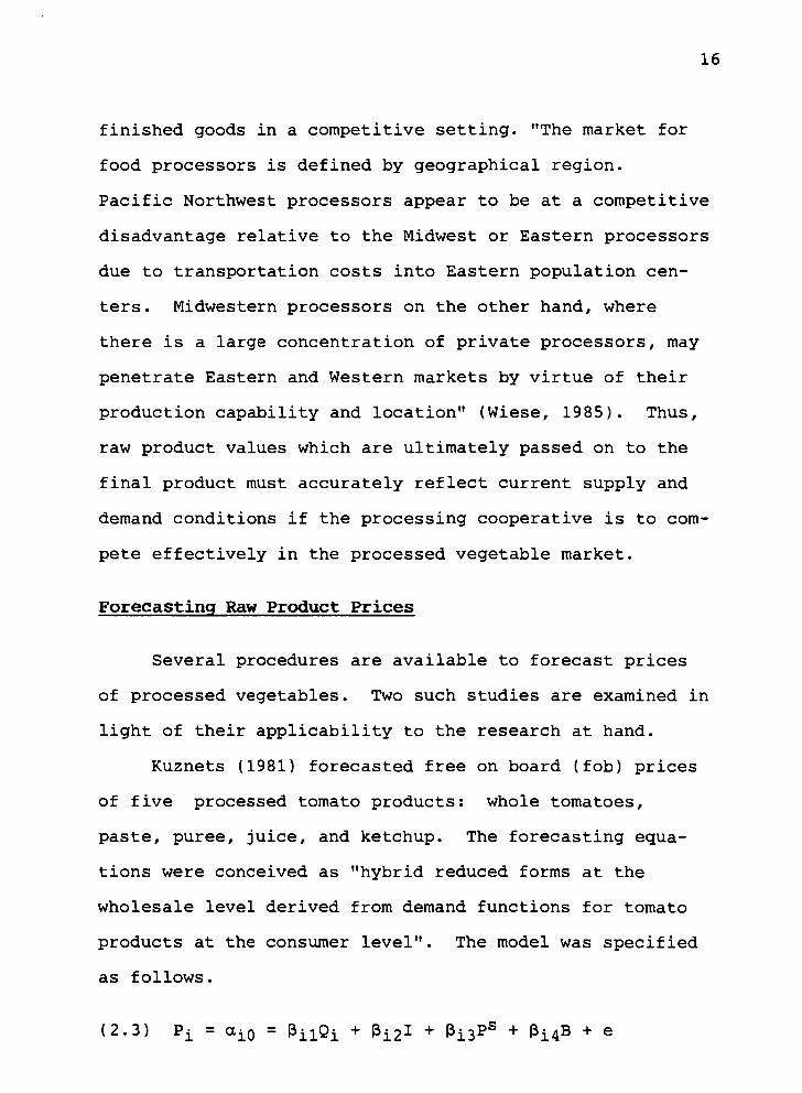
Kuznets (1981) forecasted free on board (fob) prices
of five processed tomato products: whole tomatoes,
paste, puree, juice, and ketchup. The forecasting equa-
tions were conceived as "hybrid reduced forms at the
wholesale level derived from demand functions for tomato
products at the consumer level". The model was specified
as follows.
(2.3) Pi = ai0 = PiuQi + pi2l + Pi3Ps + (^B + e
17
P^ = a national average f.o.b. price of a given product,
in dollars per case, deflated by the CPI;
Qi = pack plus carry in inventory in thousands of actual
cases;
I = disposable personal income, in billions of dollars,
deflated by the CPI;
Ps = the CPI which served as the price of a substitute;
B = a binary variable;
e = an error term.
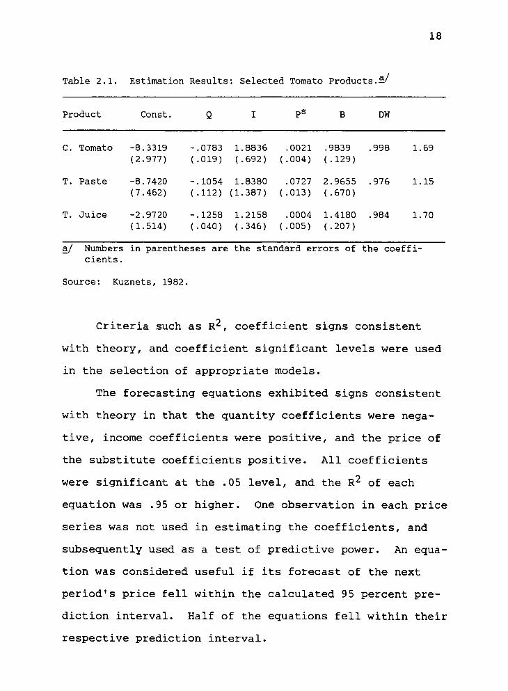
Several alternative quantity variables were tested at
the state and national level. Since substantial quan-
tities of tomato products were produced outside of
California during the time period of investigation (1960-
1980), national quantity variables were used. The deter-
minants of demand were disposable personal income, the
consumer price index (which served as the price of
substitutes), and a binary "dummy" variable to permit
treatment of rapidly rising prices beginning in 1973. A
sample of the estimation results obtained using ordinary
least squares is presented in Table 2.1.
18
Table 2.1. Estimation Results: Selected Tomato Products.—' a/
Product Const. DW
c. Tomato -8.3319 (2.977)
T. Paste -8.7420 (7.462)
T. Juice -2.9720 (1.514)
-.0783 1.8836 .0021 .9839 .998 1.69 (.019) (.692) (.004) (.129)
-.1054 1.8380 .0727 2.9655 .976 1.15 (.112) (1.387) (.013) (.670)
-.1258 1.2158 .0004 1.4180 .984 1.70 (.040) (.346) (.005) (.207)
a/ Numbers in parentheses are the standard errors of the coeffi- cients.
Source: Kuznets, 1982,
Criteria such as R^, coefficient signs consistent
with theory, and coefficient significant levels were used
in the selection of appropriate models.
The forecasting equations exhibited signs consistent
with theory in that the quantity coefficients were nega-
tive, income coefficients were positive, and the price of
the substitute coefficients positive. All coefficients
were significant at the .05 level, and the R^ of each
equation was .95 or higher. One observation in each price
series was not used in estimating the coefficients, and
subsequently used as a test of predictive power. An equa-
tion was considered useful if its forecast of the next
period's price fell within the calculated 95 percent pre-
diction interval. Half of the equations fell within their
respective prediction interval.
19
Kuznet's results are encouraging. The explanatory
variables all exhibit signs which are consistent with
economic theory. All coefficients were significant at the
.05 level, and the explanatory power of the equations is
quite good.
From these results it appears possible to forecast
industry average f.o.b. prices. The Willamette Valley
processing cooperative differs from Kuznet's research in
that the dependent variable will be a firm specific net
returns for a Willamette Valley vegetable processor rather
than industry fob prices. The independent variables and
their functional form are similar to the ones proposed in
this study.
Previous work was conducted by Wiese to forecast raw
product values for Willamette Valley vegetable coopera-
tives. An econometric model and an exponential smoothing
process were used to forecast net returns/acre to the
cooperative, for both canned and frozen beans and corn.
In Wiese's research the dependent variable was calcu-
lated on a pool year basis. Different quantity variables
and functional forms were tested in developing the firm-
specific supply figures. The approach taken in Wiese's
research was to forecast supplyt+i using a system of
recursive equations estimated by ordinary least squares.
The determinants of demand were personal disposable income
and the price of a substitute. The substitute for the
20
canned line was its frozen counterpart, and for the frozen
line its fresh counterpart was used. Lagged expenditures
on plant and equipment were used as a proxies for dis-
posable personal income. A lagged income variable was
also tested and the variable producing the best fit was
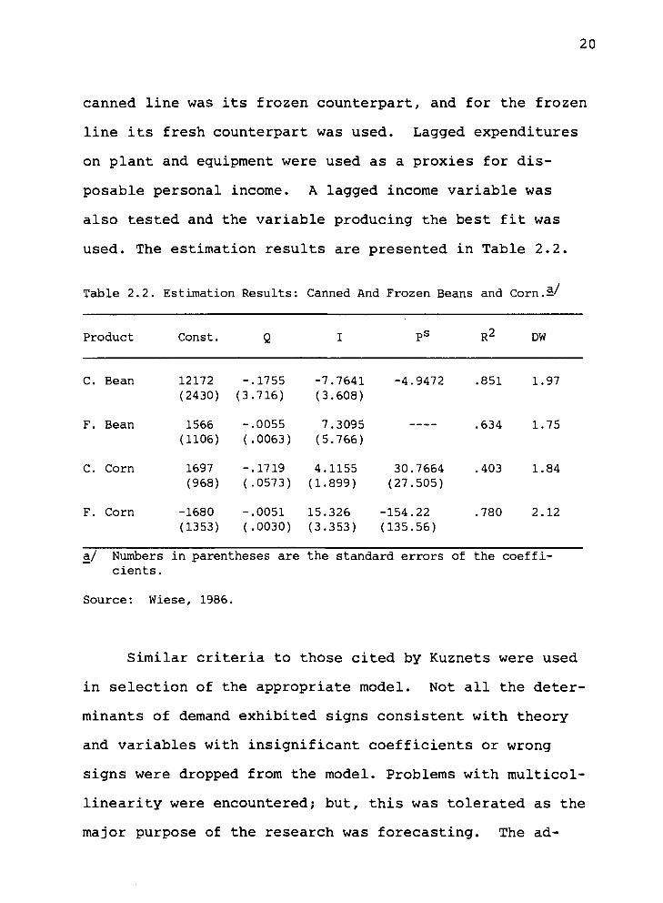
used. The estimation results are presented in Table 2.2.
Table 2.2. Estimation Results: Canned And Frozen Beans and Corn.—'
Product Const. 0 1 Ps R2 DW
-4.9472 .851 1.97
.634 1.75
30.7664 .403 1.84 (27.505)
-154.22 .780 2.12 (135.56)
a/ Numbers in parentheses are the standard errors of the coeffi- cients.
Source: Wiese, 1986.
Similar criteria to those cited by Kuznets were used
in selection of the appropriate model. Not all the deter-
minants of demand exhibited signs consistent with theory
and variables with insignificant coefficients or wrong
signs were dropped from the model. Problems with multicol-
linearity were encountered; but, this was tolerated as the
major purpose of the research was forecasting. The ad-
C. Bean 12172 - .1755 -7.7641 (2430) (3 .716) (3.608)
F. Bean 1566 _ .0055 7.3095 (1106) ( .0063) (5.766)
C. Corn 1697 - .1719 4.1155 (968) ( .0573) (1.899)
F. Corn -1680 - .0051 15.326 (1353) ( .0030) (3.353)
21
justed R^s ranged from .403 to .851, suggesting a wide
range of explanatory power for the various models. Two
observations were used as a test of the model's forecast-
ing power. The results over this time interval were
mixed; overall, the econometric model did not forecast
well for the test period.
The results of this study are not as encouraging as
those of Kuznets. The estimators for canned beans and
frozen corn forecasting models, however, perform better
than the current method used by the cooperative, for es-
tablishing price of raw products. In light of the results
for these two commodities, it appears possible to forecast
raw product values of select vegetable crops. The
econometric model developed in this research will draw
upon the methodology used by both Wiese and Kuznets in
specification of both the explanatory and dependent vari-
ables.
Econometric Model Conceptualization
Willamette Valley vegetable producers are experienc-
ing increased market competition from proprietary proces-
sors in the Midwest. Because of the interregional com-
petitive relationship national supply and demand condi-
tions are used to forecast a value of the raw product in
Oregon. The dependent variable (raw product value) for
this study is derived from the finished product value. It
22
is assumed that in the long-run competitive conditions ex-
ists in the Willamette Valley retail market. Thus, there
is no profit accruing to the cooperative over time; there-
fore, net revenue less all costs of processing, handling,
and marketing yields the actual value for raw product.
This actual value over time ideally should be the same as
the economic value estimated by the cooperative.
Econometric Conceptual Model
In developing the econometric models an autoregres-
sive technique which contains lagged dependent variables
and reduced form technique will be utilized. The lost
degree of freedom with the autoregressive model will be
weighed against the explanatory power of the lagged depen-
dent variable to determine if this type of model is jus-
tified. Selection of model structure was derived from
economic theory and relationships initially developed by
the Agricultural Marketing Service (USDA/Foote, 1959).
As the model is developed in a national context.
Supply is defined as the sum of pack in year (t), and
carry-in inventory from year (t-1). These pack-i/ or can-
ner supply figures are nationwide totals for each respec-
tive vegetable crop. The determinants of demand are as-
sumed to be its own price, personal disposable income, the
1' Supply is also referred to as pack, which is the volume of vegetables processed (packed) in a given year.
23
price of substitute products, population, and a proxy for
consumer tastes and preferences (Mansfield, 1985).
Econometric Relationship
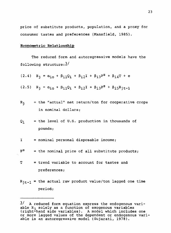
The reduced form and autoregressive models have the
following structure:!'
(2.4) Rj = aio + PiiQi + pi2I + Pi3pS + ^LA7 + e
(2.5) Rj = aio + PijQi + 3i2l + Pi3pS + Pi5Rjt-l
Rj = the "actual" net return/ton for cooperative crops
in nominal dollars;
QJL = the level of U.S. production in thousands of
pounds;
I = nominal personal disposable income;
Ps = the nominal price of all substitute products;
T = trend variable to account for tastes and
preferences;
Rjt_l = the actual raw product value/ton lagged one time
period;
!■' A reduced form equation express the endogenous vari- able Rj solely as a function of exogenous variables (right-hand side variables). A model which includes one or more lagged values of the dependent or endogenous vari- able is an autoregressive model (Gujarati, 1978).
24
e = an error term
These functional forms were applied to two processed
vegetable crops; snap beans and sweet corn.
Technical Forecasting Method
In time series analysis which utilizes econometric
methodology, the assumption is made that the series to be
forecasted has been generated by a stochastic process.
That is, a process with a structure that can be charac-
terized and explained. In the development of some
econometric models, however, there is variability in a
time series which cannot be accounted for with observable
explanatory variables (i.e. random events such as changes
in industry structure or internal management decisions of
a firm). There is a broad category of forecasting tech-
niques which attempts to account for this difficulty.
This is accomplished not in terms of a cause and effect
relationship but rather in terms of the way that random-
ness is embodied in the process (Pindyck and Rubinfield,
1976).
Common technical forecasting methods are the auto-
regressive integrated moving average (ARIMA) model and the
exponential smoothing technique. These models generate
forecasts by estimating past patterns in a time series and
projecting them into the future.
25
"In time series there are two basic ways of expressing a relationship, autoregressive and moving average. Autoregressive assumes that future values are a linear combination of past values. Moving average models on the other hand assumes that future values are a linear combination of past errors. A com- bination of the two is called ARIMA" (Makridakis and Wheelwright, 1982).
Thus, ARIMA has an advantage over exponential smooth-
ing in that forecasts are generated through identification
and diagnostic checking of certain data properties. The
data set upon which this research is based is limited to
only 25 observations, annual data (1960-1985). Box and
Jenkins (1970) derived a series of ARIMA model building
requirements. One such requirement is that a time series
data set contain a minimum of 50 observations. With the
current research there are only 25 observations and sub-
sequently the use of an exponential smoothing model is
dictated.
"Smoothing techniques are a higher form of a naive
forecasting model which assume that there is an underlying
pattern to be found in historical values of a variable
that is being forecast" (McGuigan and Moyer, 1986). These
techniques are particularly useful in accounting for ran-
dom shocks in a series which most likely cannot be cap-
tured by an econometric model.
Wiese (1985) developed such a model for Willamette
Valley vegetables. In the Wiese model the forecasting
26
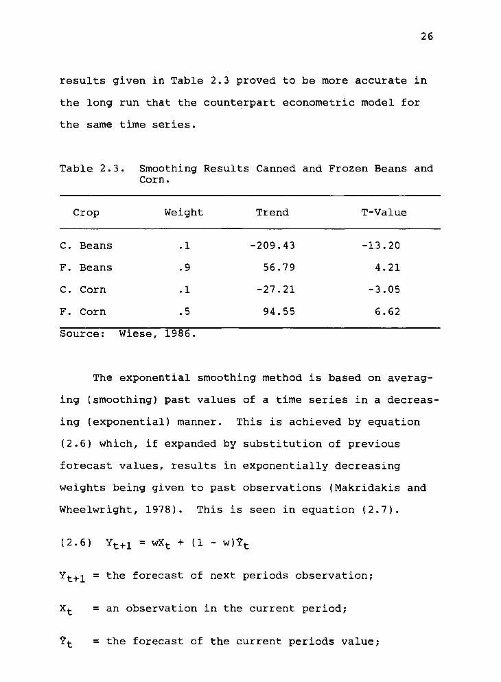
results given in Table 2.3 proved to be more accurate in
the long run that the counterpart econometric model for
the same time series.
Table 2.3. Smoothing Results Canned and Frozen Beans and Corn.
Crop Weight Trend T-Value
C. Beans .1 -209.43 -13.20
F. Beans .9 56.79 4.21
C. Corn .1 -27.21 -3.05
F. Corn .5 94.55 6.62
Source: Wiese, 1986
The exponential smoothing method is based on averag-
ing (smoothing) past values of a time series in a decreas-
ing (exponential) manner. This is achieved by equation
(2.6) which, if expanded by substitution of previous
forecast values, results in exponentially decreasing
weights being given to past observations (Makridakis and
Wheelwright, 1978). This is seen in equation (2.7).
(2.6) Yt+1 = wXt + (1 - w)?t
Yt+-L = the forecast of next periods observation;
Xt = an observation in the current period;
■?{. = the forecast of the current periods value;
27
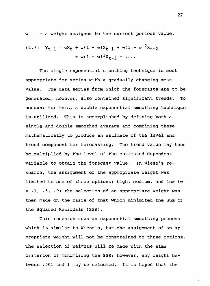
w = a weight assigned to the current periods value.
(2.7) Yt+1 = wXt + w(l - w)X.t-1 + w(l - w)2Xt_2
+ w(l - w)3Xt_3 +
The single exponential smoothing technique is most
appropriate for series with a gradually changing mean
value. The data series from which the forecasts are to be
generated, however, also contained significant trends. To
account for this, a double exponential smoothing technique
is utilized. This is accomplished by defining both a
single and double smoothed average and combining these
mathematically to produce an estimate of the level and
trend component for forecasting. The trend value may then
be multiplied by the level of the estimated dependent
variable to obtain the forecast value. In Wiese's re-
search, the assignment of the appropriate weight was
limited to one of three options; high, medium, and low (w
= .1, .5, .9) the selection of an appropriate weight was
then made on the basis of that which minimized the Sum of
the Squared Residuals (SSR).
This research uses an exponential smoothing process
which is similar to Wiese's, but the assignment of an ap-
propriate weight will not be constrained to three options.
The selection of weights will be made with the same
criterion of minimizing the SSR; however, any weight be-
tween .001 and 1 may be selected. It is hoped that the
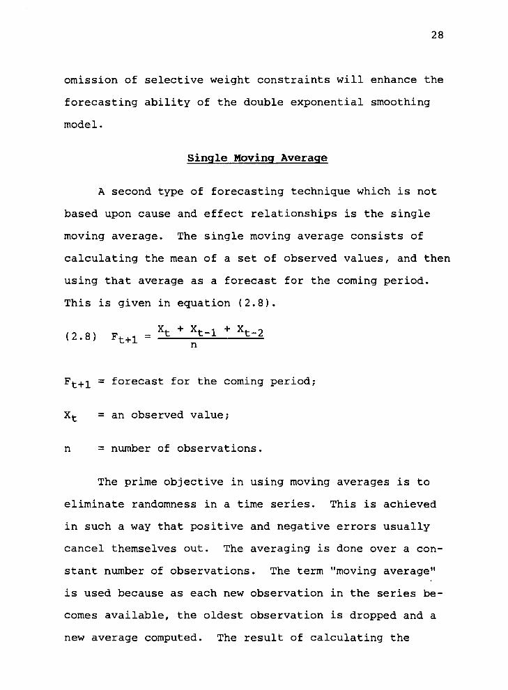
28
omission of selective weight constraints will enhance the
forecasting ability of the double exponential smoothing
model.
Single Moving Average
A second type of forecasting technique which is not
based upon cause and effect relationships is the single
moving average. The single moving average consists of
calculating the mean of a set of observed values, and then
using that average as a forecast for the coming period.
This is given in equation (2.8).
(2.8) Ff+n = _t ±=1 tzl L.-rj. n
Ft+i = forecast for the coming period;
Xt = an observed value;
n = number of observations.
The prime objective in using moving averages is to
eliminate randomness in a time series. This is achieved
in such a way that positive and negative errors usually
cancel themselves out. The averaging is done over a con-
stant number of observations. The term "moving average"
is used because as each new observation in the series be-
comes available, the oldest observation is dropped and a
new average computed. The result of calculating the
29
moving average over a set of data points, is a new series
of numbers with "little" randomness (Makridakis and
Wheelwright, 1979). Often times the use of moving average
techniques are employed with data where trends are in-
volved. The dependent data series for which forecasts in
this research are being made is a series in which trends
exist. For this reason the moving average method of gen-
erating forecasts will be utilized along with those pre-
viously mentioned.
Composite Forecasting
Three forecasting methods have been outlined with
different justification for their use. Any or all of
these techniques have the possibility of making large er-
rors for a given time period due to presumed existence of
both random and stochastic variables. Composite forecast-
ing is a method of combining alternative forecasting
models in an effort to remove the likelihood of large mis-
takes based on the forecasts of a single model. In
general terms, the use of composite forecasting can find
its theoretical justification in risk literature.
Bessler and Brandt (1979) developed three alternative
forecasting procedures for hog cattle and broiler prices.
The alternative methods of forecasting were an econometric
model, moving average (ARIMA) process, and expert opinion.
Three alternative composite forecasting models were then
30
developed. These models were essentially combinations of
the results generated from the individual methods. The
differences among the composite forecasting techniques are
in the weighing schemes given to the forecasts of the
other models. Three alternative weighting procedures were
utilized: (1) minimum variance, (2) adaptive, and (3)
simple average. Empirical results from this study are
given in Table 2.4.
The empirical results from the three alternative com-
posite forecasts, generated results which were at least as
good as any of the individual forecasts. The MSE of the
best individual forecasting method was compared with that
of the best composite for each of the three commodities.
The composite forecast errors of the three commodities
averaged 14 percent lower than the errors of the best in-
dividual forecasts. In addition, comparing the MSE of the
worst individual forecasts with that of the worst in-
dividual composite forecast shows that the composite error
resulted in an average of 42 percent lower variance for
the three commodities.
Bessler and Brandt's results suggest that composite
forecasts can be efficient methods of combining predict-
ions into an improved forecast. Composite methodology
relies on forecasts from individual models which can be
used in a simple average or with alternative weighing
schemes. Three alternative forecasting methods have been
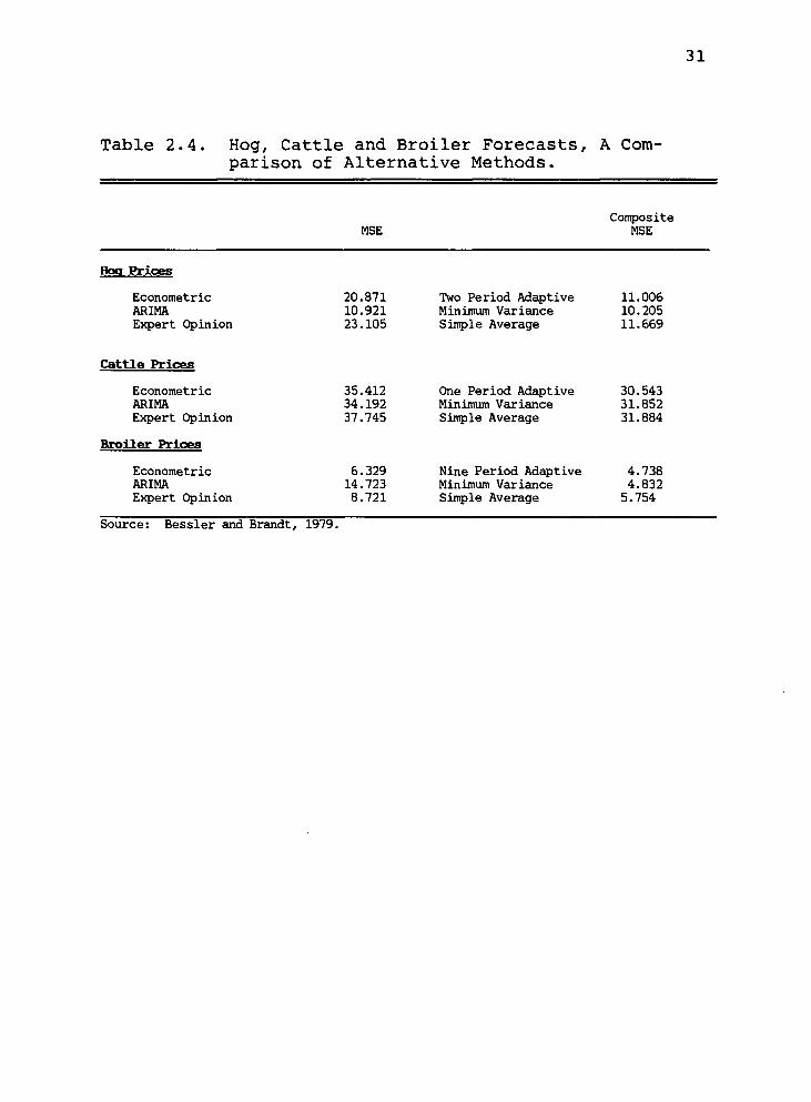
Table 2.4. Hog, Cattle and Broiler Forecasts, A Com- parison of Alternative Methods.
MSE Composite
MSE
Econometric ARIMA Expert Opinion
20.871 Two Period Adaptive 11.006 10.921 Minimuin Variance 10.205 23.105 Simple Average 11.669
Cattle Prices
Econometric ARIMA Expert Opinion
Broiler Prices
35.412 One Period Adaptive 30.543 34.192 Minimum Variance 31.852 37.745 Simple Average 31.884
31
Hog Prices
Econometric ARIMA Expert Opinion
6.329 Nine Period Adaptive 4.738 14.723 Minimum Variance 4.832 8.721 Simple Average 5.754
Source: Bessler and Brandt, 1979.
32
previously outlined for application in this research
directed towards processing cooperatives. A composite
forecast will also be developed, utilizing alternative
weighting schemes.
Summary
At present, the representative processing cooperative
operates on a single pool basis. Under this pool design,
a method is necessary to allocate net revenues to grower-
members. Raw product valuation is the basis for this pay-
ment calculation. A discussion of payment calculations
and the resulting implications among growers within a
single-pool was identified.
A description of the pricing mechanisms for both the
raw product and processed goods market has been iden-
tified. The use of the current raw product valuation
technique utilized by cooperative management, and the
resulting implications for misallocated acreage and inap-
propriate production levels was discussed. The current
method for assigning a value to raw products is essen-
tially a one period naive forecast. The hypothesis was
made that more efficient alternative forecasting methods
for raw product valuation could be developed. Alternative
raw product value forecasting methods were developed based
on an assessment of the relevant literature and theoreti-
cal relationships.
33
CHAPTER III
MODEL SPECIFICATION
This chapter explains design of alternative raw
product valuation procedures. First, the time frame for
production and marketing decisions by the cooperative are
linked to the subsequent raw product forecast date. The
variables to be forecasted on a pool year basis are iden-
tified along with a description of their respective ex-
planatory econometric models. A discussion of how single
pool payments will be evaluated for alternative economic
value forecasters is also given. The chapter concludes
with a discussion of the data and the units used.
Accounting Period
A description of the cooperative's accounting period
is necessary to understand the organization of data used
in the forecasting procedures. Two alternative time
frames confront the cooperative in forecasting raw product
value. The 12 month fiscal year interval generates data
which is used for internal planning. Secondly the 24
month pool year interval, extending from harvest until the
processed product is sold to the succeeding pool, from
which grower-member payment calculations are estimated.
The cooperative's fiscal year runs from April 1 to March
31 of the following year. A single pool accounting period
34
covers two years so the pool that opened April 1, in year
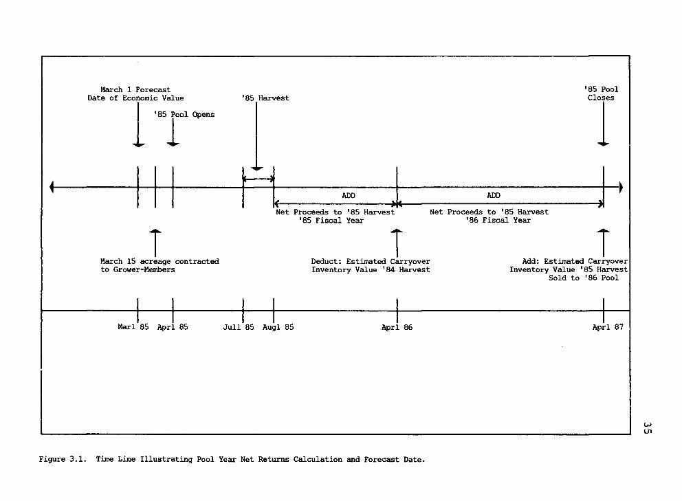
t will close March 31, in year t+2 (Figure 3.1, page 35).
The harvest season for snap beans and sweet corn the
two products under consideration in this study extends
from early July through the end of August.i' Processing
begins during the harvest season and sales of processed
products begin immediately. Roughly 60 percent of the
processed product is still unsold at the end of the first
fiscal year and sales continue through the second fiscal
year. Any product left in inventory at the end of the
pool year is transferred to the succeeding pool (Smith,
1984). Estimated sales value of the transferred products
left in inventory at this time is credited to the pool
which is closed.
Pool-Year Econometric Model
The Dependent Variable
In this research net returns per ton is treated as
the dependent variable. These returns were calculated on
a pool year basis using the financial records of the
cooperative over the time period 1960 through 1985
(Subaei, 1984). These records list net returns on a fis-
i/ Snap green beans and sweet corn are analyzed in this study.
March 1 Forecast Date of Economic Value ■85 Harvest
•85 Pool Closes
'85 Pool Opens
1 I ADD ADD
-»t
T Net Proceeds to '85 Harvest
'85 Fiscal Year Net Proceeds to '85 Harvest
•86 Fiscal Year
March 15 acreage contracted to Grower-Menibers
T Deduct: Estimated Carryover Inventory Value '84 Harvest
T Add: Estimated Carryover
Inventory Value '85 Harvest Sold to '86 Pool
Marl 85 Aprl 85 Jull 85 Augl 85 Aprl 86 Aprl 87
Figure 3.1. Time Line Illustrating Pool Year Net Returns Calculation and Forecast Date.
36
cal year basis, established economic values^/ and the es-
timated carry-over inventory values formed at the close of
a pool. For example, for snap beans harvested in July
through August of 1985, the net returns realized during
the April 1 through March 31 1985 fiscal year, were added
to the net returns realized during the 1986 fiscal year to
determine net returns payable to the 1985 pool. An ad-
justment for carry-over inventory is also made. This pro-
cedure is illustrated in Figure 3.1, using the 1985 pool
as an example. The estimated carry-over inventory value
formed at the close of the 1985 pool is added to the 1985
pool net returns, and the estimated carry-over inventory
value formed at the end of the 1984 pool (paid out of the
1985 pool) is subtracted out (Weise, 1985).
This calculation yields net returns to products on a
pool year basis. Total tons of each respective commodity
the cooperative processes were then divided into total net
returns of that commodity to yield net returns per ton.
The calculation of this value yields returns to coopera-
tives at the wholesale level, less all costs of processing
and selling that product. A raw product's "actual value"
is taken to be net returnes per ton at the wholesale
1/ Established economic values are the basis for raw product payments to grower-members. These values are forecasted in March of each year by cooperative manage- ment.
37
level. These procedures were carried out for both snap
beans and sweet corn serving as the dependent variable to
forecasted in this study.—'
The Explanatory Variables
Supply. The supply of the processed product for the
forecast interval comes from two sources; pack in year t
and carry-over inventory from year t-1. Summing these
yields the total volume of processed vegetables available
after harvest in the finished goods market. Willamette
Valley vegetable processors have experienced increased
competition from other regions for market share in the
Northwest. Thus, national pack and carry-over inventory
levels were used to estimate product value.
The calculation yielding total pack available was
carried out separately for the canned and frozen product
lines. These figures were included individually as ex-
planatory variables in the econometric model. The in-
dividual figures for the frozen and canned lines were then
combined to calculate total pack figures for each com-
modity.
A Chow test was then used to determine if the two
sets of supply coefficients (canned and frozen combined
verses canned and frozen individually) used in the
^7 Net Returns = Total Sales - [Processing, Selling and Shipping Costs] + an adjustment for carry-over inventory.
38
regressions were statistically the same. This was in fact
proven to be the case. This same procedure was also
carried out for incorporation of either one or the other
of the canned or frozen lines for inclusion in the model
individually. For snap beans the pack of the canned line
is included for the supply figure as the t-statistic
proved to have higher degree of significance individually
verses the canned and frozen lines combined. A Chow test
justified the use of only incorporating the canned pack
level in the model for snap beans. The supply figure for
sweet corn on the other hand, was best represented as the
total pack level for both the frozen and canned processed
goods combined.
Demand. The determinants of demand for the finished
goods are hypothesized to be personal disposable income
and the price of a demand substitute product. Several al-
ternative substitute products were tested in both nominal
and real terms. The respective t-statistics and adjusted
R^s were then used in selection of an appropriate model.
The best specification utilized the consumer price index
(CPI) as the price of all substitute products. As the CPI
was included as an explanatory variable, personal dis-
posable income as well as the variable to be forecasted
were utilized in nominal verses real terms. This was the
case for both snap beans and sweet corn.
39
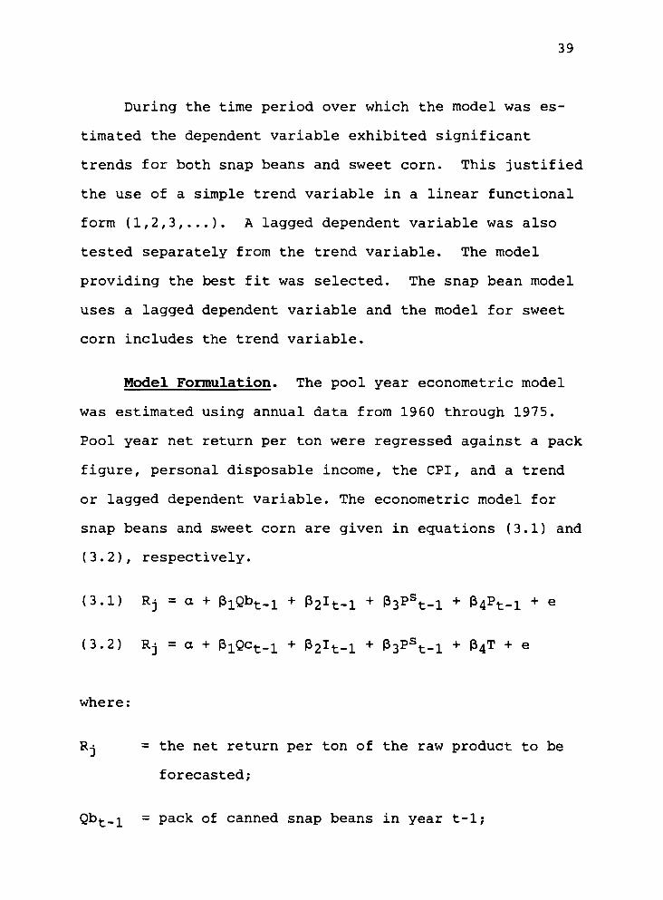
During the time period over which the model was es-
timated the dependent variable exhibited significant
trends for both snap beans and sweet corn. This justified
the use of a simple trend variable in a linear functional
form (1,2,3,...). A lagged dependent variable was also
tested separately from the trend variable. The model
providing the best fit was selected. The snap bean model
uses a lagged dependent variable and the model for sweet
corn includes the trend variable.
Model Formulation. The pool year econometric model
was estimated using annual data from 1960 through 1975.
Pool year net return per ton were regressed against a pack
figure, personal disposable income, the CPI, and a trend
or lagged dependent variable. The econometric model for
snap beans and sweet corn are given in equations (3.1) and
(3.2), respectively.
(3.1) Rj = a + PxQbt.! + P2It-l + P3pSt-l + P4pt-1 + e
(3.2) Rj = a + PiQCt.! + p2It-l + P3pSt-l + P4T + e
where:
Rj = the net return per ton of the raw product to be
forecasted;
Q^t-1 = Pack of canned snap beans in year t-1;
40
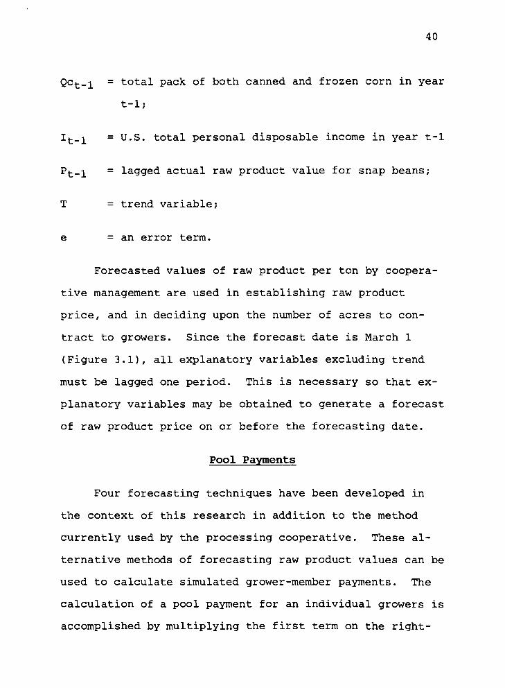
Qct_i = total pack of both canned and frozen corn in year
t-1;
It_^ = U.S. total personal disposable income in year t-1
Pt_^ = lagged actual raw product value for snap beans;
T = trend variable;
e = an error term.
Forecasted values of raw product per ton by coopera-
tive management are used in establishing raw product
price, and in deciding upon the number of acres to con-
tract to growers. Since the forecast date is March 1
(Figure 3.1), all explanatory variables excluding trend
must be lagged one period. This is necessary so that ex-
planatory variables may be obtained to generate a forecast
of raw product price on or before the forecasting date.
Pool Payments
Four forecasting techniques have been developed in
the context of this research in addition to the method
currently used by the processing cooperative. These al-
ternative methods of forecasting raw product values can be
used to calculate simulated grower-member payments. The
calculation of a pool payment for an individual growers is
accomplished by multiplying the first term on the right-
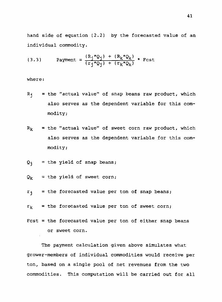
41
hand side of equation (2.2) by the forecasted value of an
individual commodity.
(3.3) Parent = 'W + 'W . Fast (r^Qj) + (rk*Qk)
where:
Rj = the "actual value" of snap beans raw product, which
also serves as the dependent variable for this com-
modity;
Rk = the "actual value" of sweet corn raw product, which
also serves as the dependent variable for this com-
modity;
Qj = the yield of snap beans;
Qk = the yield of sweet corn;
rj = the forecasted value per ton of snap beans;
r^ = the forecasted value per ton of sweet corn;
Fcst = the forecasted value per ton of either snap beans
or sweet corn.
The payment calculation given above simulates what
grower-members of individual commodities would receive per
ton, based on a single pool of net revenues from the two
commodities. This computation will be carried out for all
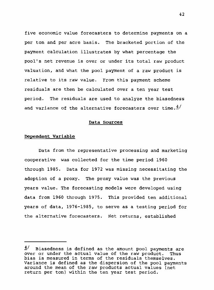
42
five economic value forecasters to determine payments on a
per ton and per acre basis. The bracketed portion of the
payment calculation illustrates by what percentage the
pool's net revenue is over or under its total raw product
valuation, and what the pool payment of a raw product is
relative to its raw value. From this payment scheme
residuals are then be calculated over a ten year test
period. The residuals are used to analyze the biasedness
and variance of the alternative forecasters over time.-i'
Data Sources
Dependent Variable
Data from the representative processing and marketing
cooperative was collected for the time period 1960
through 1985. Data for 1972 was missing necessitating the
adoption of a proxy. The proxy value was the previous
years value. The forecasting models were developed using
data from 1960 through 1975. This provided ten additional
years of data, 1976-1985, to serve as a testing period for
the alternative forecasters. Net returns, established
i/ Biasedness is defined as the amount pool payments are over or under the actual value of the raw product. Thus bias is measured in terms of the residuals themselves. Variance is defined as the dispersion of the pool payments around the mean of the raw products actual values (net return per ton) within the ten year test period.
43
economic values, carry-over inventory estimates and the
derived net returns are all expressed in nominal dollars.
Independent Variables
Canned industry inventory and pack data were obtained
from The Almanac of the Canning, Freezing and Preserving
Industries, (1959-1986). Frozen industry pack data were
also obtained from this reference; however, carry-over
data were obtained from "Suiranaries of Regional Cold
Storage Holdings," published by the USDA Statistical
Reporting Service. Canned industry levels were reported
in thousands of actual cases, while frozen levels were
reported in thousands of actual pounds.
Representative yield per acre figures were obtained
for Oregon's Polk county within the cooperatives member-
ship area, compiled by Extension Economic Information Of-
fice, at Oregon State University (1960-1985).
Personal disposable income figures were obtained from
"Economic Indicators," (1969-1985), compiled by the Coun-
cil of Economic Advisors. This variable was expressed in
billions of nominal dollars. The price of substitute
products, the (CPI), were obtained from "Outlook and
Situation," (1960-1985), with 1972 being the base year.
44
Summary
Econometric forecasting equations for raw product
values were developed for two commodities, snap beans and
sweet corn. These models were developed utilizing data
from 1960 through 1975, leaving 1976 through 1985 to serve
as test period for the various models forecasting ability.
The dependent variables for the econometric models as
well as the exponential smoothing, moving average and com-
posite techniques were obtained from the cooperative's
financial records. The econometric models were developed
by regressing the dependent variable against a pack
(supply) figure, personal disposable income, the CPI
(which served as the price of all substitute products),
and a trend or lagged dependent variable. Pool payment
calculations were then developed. These calculations will
simulate over time how grower-members would be compensated
by the cooperative based on five alternative forecasts of
economic value.
45
CHAPTER IV
RESULTS
This chapter starts with a discussion of specifica-
tion criteria used in selection of alternative forecasting
procedures. Comparative statistics which are utilized in
the evaluation of different forecasting methods are given.
Forecasts of raw product values based the econometric and
exponential smoothing models are presented and discussed.
This is followed by a discussion of simulated pool year
returns as calculated from the five alternative forecast-
ing models. The chapter concludes with an evaluation of
forecasting performance over the post-sample period using
appropriate statistical measures.
Sample Size and Forecast Interval
Financial data from the representative cooperative
for which this study is based was obtained for the period
1960 to 1985. Model estimation was then generated from
the period 1960 to 1975, allowing a ten year (1976-1985)
post-sample period for evaluation of forecasting proce-
dures and resulting pool year returns. The alternative
forecasting models were estimated and subsequently updated
each year as further data became available within the test
period.
46
The sample size for the econometric model was held
constant with 17 observations beginning in the year 1977.
As an additional year's observation became available, the
earliest data point was omitted. This was done in an ef-
fort to confine the models to periods with relative con-
stant structure. This should allow the explanatory vari-
ables to accurately reflected changes in the dependent
variable.
Model Specification Criteria
The criteria used to specify the econometric models
were the adjusted R^ values, consistency of the indepen-
dent variable coefficient signs with economic theory, sig-
nificant levels of independent variables, and considera-
tions of multicollinearity and serial correlation. The
criterion for the exponential smoothing technique was min-
imization of the SSR. Selection of the appropriate number
of periods to include in the moving average and fitting of
weights for the composite forecast were also based on the
same SSR criterion.
Comparative Statistics of Forecasters
After the model specification was complete, criteria
had to be chosen in which comparisons of alternative
forecasters could be made. When forecasting over several
periods, a series of error values will be generated over
47
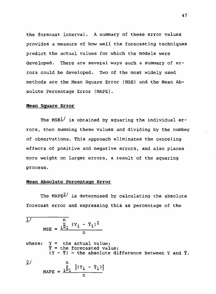
the forecast interval. A summary of these error values
provides a measure of how well the forecasting techniques
predict the actual values for which the models were
developed. There are several ways such a summary of er-
rors could be developed. Two of the most widely used
methods are the Mean Square Error (MSE) and the Mean Ab-
solute Percentage Error (MAPE).
Mean Square Error
The MSEi' is obtained by squaring the individual er-
rors, then summing these values and dividing by the number
of observations. This approach eliminates the canceling
effects of positive and negative errors, and also places
more weight on larger errors, a result of the squaring
process.
Mean Absolute Percentage Error
The MAPE^/ is determined by calculating the absolute
forecast error and expressing this as percentage of the
1/ n _ i^ <*i " *i)2
MSE n
where: Y = the actual value; "? = the forecasted value; (Y - "?) = the absolute difference between Y and "?.
2/ n , i?, (Yi " *i>| MAPE = i=±
n
48
forecasts. Interpretation of the MAPE is more intuitive
than the MSE. A MAPE of eight percent which represents
the magnitude of the forecast error, for example, is
easier to interpret than a MSE of 12456. Both of these
comparative statistics are absolute measures; however, the
MAPE gives equal weight to all errors. Based on the ease
of interpretation and different weighing schemes both
measures will be used.
Parameter Evaluation of Econometric
and Exponential Smoothing Models
Econometric Model: Snap Beans
Table 4.1 presents a summary of the estimation
results for the snap bean econometric model which was
specified in Chapter III (EQ 3.1). Variables for this
model are defined on page 39. The results in complete
form may be referenced in Appendix A. Pool-year net
returns per ton serves as the dependent variable. Numbers
in parentheses are standard errors of the coefficients.
Interpretation
The results in Table 4.1 contain multicollinearity
between disposable income and the price of substitute
Table 4.1
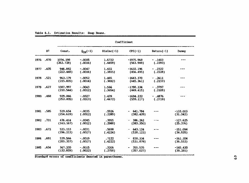
Table 4.1. Estimation Results: Snap Beans.
R2
Coefficient
Const. QON*"1) Dislnc(-l) CPI(-l) Return(-l) Dumny
1976 .470 1094.198 (263.728)
-.0005 (.0016)
1.6722 (.4459)
-1975.968 (563.949)
- .1403 (.2393)
—
1977 .435 946.882 (222.448)
-.0047 (.0016)
1.432 (.3815)
-1632.196 (456.495)
- .2322 (.2228)
1978 .521 963.179 (215.835)
-.0052 (.0014)
1.465 (.3692)
-1643.370 (445.361)
- .2611 (.2133)
1979 .627 1007.997 (210.544)
-.0043 (.0012)
1.566 (.3654)
-1798.334 (449.415)
- .3797 (.2108)
1980 .488 929.846 (252.805)
-.0027 (.0013)
1.439 (.4472)
-1694.222 (559.117)
- .4876 (.2719)
———
1981 .585 519.654 (154.619)
-.0035 (.0012)
.5926 (.2289)
- 641.784 (382.409)
— -133.003 (31.042)
1982 .731 476.414 (143.167)
-.0045 (.0012)
.3955 (.2988)
- 386.262 (383.350)
-127.625 (25.376)
1983 .672 523.153 (196.213)
-.0031 (.0017)
.5698 (.4224)
- 643.124 (538.123)
-151.094 (34.835)
1984 .691 539.566 (203.357)
-.0019 (.0017)
.7122 (.4222)
- 838.334 (531.879)
-161.304 (36.553)
1985 .654 347.200 (132.859)
-.0015 (.0022)
.3206 (.2758)
- 355.535 (357.027)
-145.420 (38.281)
Standard errors of coefficients denoted in parentheses. vo
50
products (CPI). The coefficient of correlation between
these variables is .95. The presence of multicollinearity
was tolerated, as it is not so important to assess the in-
dividual affects of each explanatory variable, but rather
that the explanatory variables collectively may explain
the behavior of the dependent variable. It is necessary
to assume that the pattern of multicollinearity between
the two variables in question will remain the same into
the future.
As the major purpose of this research is to forecast
raw product values, serial correlation is of greater con-
cern than multicollinearity. Under the presence of serial
correlation there is a loss of efficiency, in that the
standard errors obtained from the least-squares regression
will be larger than what could have feasibly been ob-
tained. The regression estimates will still be unbiased;
however, ordinary least squares standard error estimates
will be biased downward. This leads to the conclusion
that the parameter estimates are more precise than they
actually are, resulting in larger variances when compared
with the predictions based on some other estimators.
The econometric model developed for snap beans was
autoregressive (i.e. the dependent variable was lagged and
used as an explanatory variable). In this situation the
standard measure for serial correlation (Durbin-Watson
statistic) cannot be utilized. Instead the Durbin-h
51
statistic may be used. Over the estimation period a
Durbin-h of -0.56 was indicated. This resulted in accept-
ing the null hypothesis at a 90 percent confidence inter-
val of no serial correlation.
The explanatory variables all exhibit signs consis-
tent with economic theory, and are significant at the .01
level excluding lagged returns. Lagged returns were left
in the model under the assumption that its explanatory
power would improve for subsequent forecasts.
In 1980 the processing cooperative entered a period
of rapid expansion, resulting in large losses to certain
commodities for a period of two to three years. Based on
this a dummy variable was included in forecast models sub-
sequent to 1980 and lagged returns dropped. Justification
for this was the assumption that none of the explanatory
variables could accurately reflect the profit impacts of
changing management practices strictly internal to the
cooperative.
The adjusted R^ values range from .47 to .73 within
the ten year test period, suggesting a wide range of ex-
planatory power.
Econometric Model; Sweet Corn
Table 4.2 presents a summary of the estimation
results for the sweet corn model specified in Chapter III
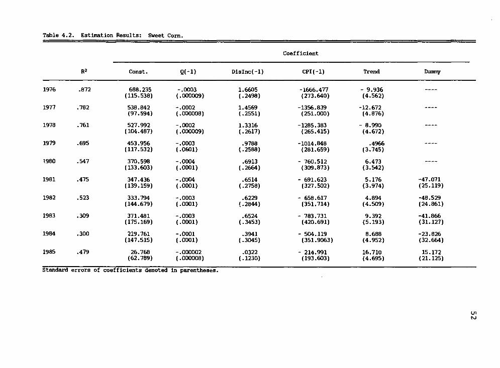
Table 4.2. Estimation Results: Sweet Corn.
Coefficient
R2 Const. Q(-l) Dislnc(-l) CPI(-l) Trend Dunny
1976
1977
1978
1979
1.980
1981
1982
1983
1984
1985
.872
.782
.761
.695
.547
.475
.523
.309
.300
.479
688.235 (115.538)
538.842 (97.594)
527.992 (104.487)
453.956 (117.532)
370.598 (133.603)
347.436 (139.159)
333.794 (144.679)
371.481 (175.169)
219.761 (147.515)
26.768 (62.789)
-.0003 (.000009)
-.0002 (.000008)
-.0002 (.000009)
-.0003 (.0601)
-.0004 (.0001)
-.0004 (.0001)
-.0003 (.0001)
-.0003 (.0001)
-.0001 (.0001)
-.000002 (.000008)
1.6605 (.2498)
1.4569 (.2551)
1.3316 (.2617)
.9788 (.2588)
.6913 (.2664)
.6514 (.2758)
.6229 (.2844)
.6524 (.3453)
.3941 (.3045)
.0322 (.1230)
-1666.477 (273.640)
-1356.839 (251.000)
-1285.383 (265.415)
-1014.848 (281.659)
- 760.512 (309.873)
- 691.623 (327.502)
- 658.617 (351.714)
- 783.731 (420.691)
- 504.119 (351.9063)
- 214.991 (193.603)
- 9.936 (4.562)
-12.672 (4.876)
- 8.990 (4.672)
.4966 (3.745)
6.473 (3.542)
5.176 (3.974)
4.894 (4.509)
9.392 (5.193)
8.688 (4.952)
16.710 (4.695)
-47.071 (25.119)
-48.529 (24.861)
-41.866 (31.127)
-23.826 (32.664)
15.172 (21.125)
Standard errors of coefficients denoted in parentheses.
on to
53
(Equation 3.2). Variables for this model are defined on
page 38. The results in complete form may be found in Ap-
pendix A. Pool-year net returns/ton serves as the depen-
dent variable. Numbers in parentheses are standard errors
of the coefficients.
Interpretation
The results in Table 4.2 are similar to those in
Table 4.1 in that multicollinearity is also present. The
presence of multicollinearity for sweet corn is more
severe than the condition exhibited with snap beans. Dis-
posable personal income being correlated with quantity,
trend, and the CPI variable. Correlation coefficients are
.94, .94, and .95 respectively. In addition the CPI was
correlated with the trend variable exhibited by a correla-
tion coefficient of .95. The presence of multicol-
linearity was again tolerated, as forecasting is the major
purpose of these models. Serial correlation apparently
was not a factor since the Durbin-Watson statistic of 2.65
allows retention of a null hypothesis that there is no
serial correlation.
The explanatory variable coefficients all exhibited
signs consistent with economic theory, and were sig-
nificant to the .01 level. A dummy variable was added to
the model in 1981 based on the same reasoning outlined un-
der snap beans. Within the ten year forecasting period
54
the adjusted R^ values ranged from a high of .87 to a low
of .30. This wide range of values is probably attributed
to changes in cooperative management practices, which can-
not be accurately reflected by forecasting variables ex-
ternal to the cooperative.
Exponential Smoothing Results
Table 4.3 presents the estimation results of the ex-
ponential smoothing model for both snap beans and sweet
corn specified in Chapter III (EQ 2.6, page 26). Pool-
year net returns per ton is the dependent variable.
Interpretation
Weights were systematically chosen between .001 and
.999 and the SSR calculated. The weight which minimized
the SSR was chosen for each year as additional data became
available. The low values of the weights illustrates the
stationarity of the net returns series after the trend has
been taken out. The lower the weight, the greater the em-
phasis placed on the net return value immediately preced-
ing the forecast. This may be seen by the smoothing model
specified in (EQ 2.6). The negative trend values for snap
beans illustrate declining net returns towards the end of
the sample period.
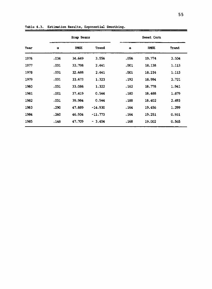
55
Table 4.3. Estimation Results, Exponential Smoothing.
Snap Beans Sweet Com
Year a RMSE Trend a RMSE Trend
1976 .034 34.649 3.556 .056 19.774 2.504
1977 .001 32.798 2.441 .001 18.138 1.113
1978 .001 32.688 2.441 .001 18.234 1.113
1979 .001 33.673 1.323 .192 18.994 2.721
1980 .001 33.086 1.322 .162 18.778 1.941
1981 .001 37.419 0.544 .180 18.488 1.879
1982 .001 39.984 0.544 .188 18.402 2.493
1983 .290 47.889 -14.930 .164 19.456 1.299
1984 .260 46.934 -11.773 .164 19.251 0.931
1985 .148 47.709 - 3.404 .168 19.002 0.565
56
Pool Year Returns
The research objectives for this analysis focuses on
five alternative raw product valuation forecasting
techniques: (1) economic value which is the forecasted
value of raw product by cooperative management and the
current basis for grower-member pool payment, (2) econ-
ometric, (3) exponential smoothing, (4) three period
moving average, and (5) a composite forecast. The
development of these models was the first primary objec-
tive. The second objective is to simulate a single pool
of commodities including snap beans and sweet corn based
on the alternative forecasters of raw product value. This
was accomplished by calculating pool-year returns per ton
and per acre utilizing the methodology given in Chapters
II and III. The results of these pool year calculations
are given in Appendix B. Select comparative statistics
are given in Table 4.4.
Evaluation of Forecasting Techniques
Evaluation Procedure
The ten year post-sample period will provide the
basis for evaluation of the different forecasting tech-
niques and their subsequent effects on pool year returns.
The sample period from which the models were developed is
ignored. The primary concern is future applications for
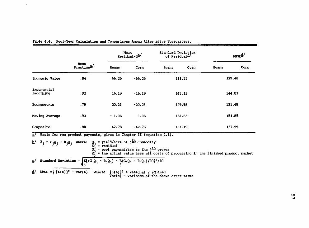
Table 4.4. Pool-Year Calculation and Comparisons Among Alternative Forecasters.
Mean , Fractions/
Mean , , Residual-22/
Beans Com
Standard Deviation of Residual2^
Beans Com
RMSE d/
Beans Corn
Economic Value
Exponential Smoothing
Econometric
Moving Average
Composite
.84
.92
.79
.93
.88
66.25
16.19
20.23
1.36
42.78
-66.25
-16.19
-20.23
1.36
-42.78
111.25
143.12
129.93
151.85
131.19
129.48
144.03
131.49
151.85
137.99
a/Basis for raw product payments, given in Chapter II (equation 2.1).
b/ Xi = GiQ1 - RiQ1 where: Q.= = yield/acre of j— conmodity J J J J J Xi = residual
Gl = pool payment/ton to the j— grower RJ = the actual value less all costs of processing in the finished product market
c/ Standard Deviation = I £[(6^ - R^Qj) - £(6^ - RjQ.p/lop/lO
d/ RMSE =\ [E(e)]2 + Var(e) where: [E(e)]2 = residual-2 squared Var(e) = variance of the above error terms
58
cooperative management; therefore all attention is focused
on ex ante descriptive statistics and ex post evaluation
is ignored. Evaluation procedures will include compara-
tive statistics, graphical analysis, and comparison of
pool-year returns and their associated biasedness and
variances.
Forecasting Comparative Statistics: One or more of
the alternative forecasters developed in the context of
this research proved superior to the economic values ap-
plied by the cooperative, for both commodities. For snap
beans, the composite forecaster out performs all others,
as indicated by its lower MSE and MAPE. The moving
average and exponential smoothing models also performed
well over the forecast horizon when compared to the
econometric and economic value models (Table 4.5)
The MSE and MAPE show accurate forecasts for the
economic value assigned to corn; however, the moving
average produces an even better fit to the dependent vari-
able. The composite and exponential smoother also provide
encouraging results.
When taking both product lines (snap beans and sweet
corn) into account the three year moving average produces
better forecasts than any other technique tested. The
econometric model produces the poorest fit to the data as
measured by the MSE and MAPE.
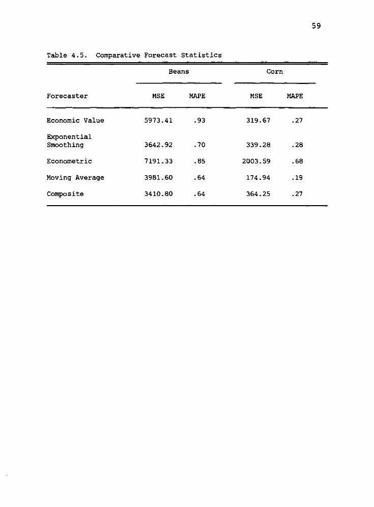
59
Table 4.5. Comparative Forecast Statistics
Beans Corn
Forecaster MSE MAPE MSE MAPE
Economic Value 5973.41 .93 319.67 .27
Exponential Smoothing 3642.92 .70 339.28 .28
Econometric 7191.33 .85 2003.59 .68
Moving Average 3981.60 .64 174.94 .19
Composite 3410.80 .64 364.25 .27
60
Graphical Analysis. A graph plot of the forecasts
provides a visual method for tracking the individual
models over time. Major fluctuations (turning points) and
general trends are more evident with graphical analysis.
Figure 4.1 illustrates the net returns, labeled actual,
and the five alternative forecasters for snap beans.
Figure 4.2 contains a comparable illustration for sweet
corn.
Turning points are not consistently predicted by any
individual forecast method for either commodity on a
regular basis. The models which perform the best in this
regard are the econometric and composite. The moving
average and exponential smoothing methods will routinely
miss major fluctuations in the data, as dictated by their
functional form. These techniques require a downward or
upward change in the data before a major shift in the
forecast may be realized. Thus, directional change in the
forecast will lag at least one period.
In tracking general trends in the data the moving
average and exponential smoothing models out perform the
formal techniques for both commodities over the entire
range of the test period.
Comparison of Pool-year Returns
The rationalization for construction of single com-
modity pools is based upon variability in returns. Single
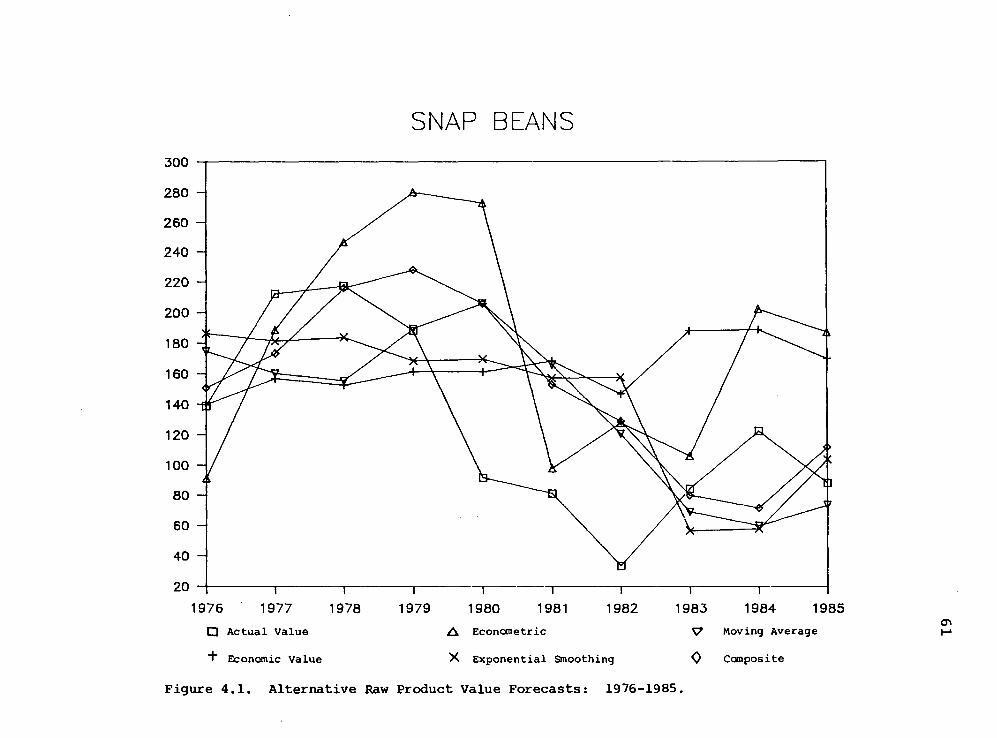
SNAP BEANS 300
20 T T T
1976 1977
□ Actual Value
"r Econcwiic Value
1978 1982 1979 1980 1981
A Econometric
X Exponential Smoothing
Figure 4.1. Alternative Raw Product Value Forecasts: 1976-1985
1983 1984 1985
^7 Moving Average
0 Composite
a\
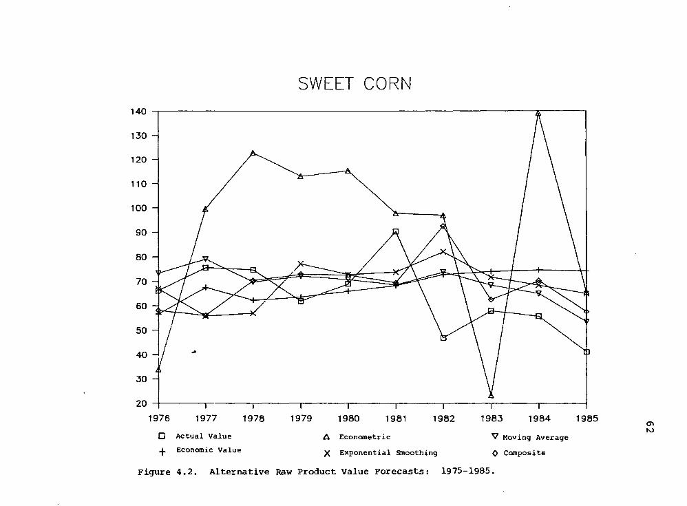
SWEET CORN 140
1976 1977 1978 1979 1980 1981 1
D Actual Value A Econometric
^. Economic Value X Exponential Smoothing
1982 1983 1984 1985
^7 Moving Average
0 Composite
Figure 4.2. Alternative Raw Product Value Forecasts: 1975-1985.
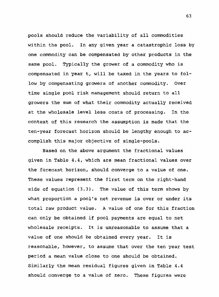
63
pools should reduce the variability of all commodities
within the pool. In any given year a catastrophic loss by
one commodity can be compensated by other products in the
same pool. Typically the grower of a commodity who is
compensated in year t, will be taxed in the years to fol-
low by compensating growers of another commodity. Over
time single pool risk management should return to all
growers the sum of what their commodity actually received
at the wholesale level less costs of processing. In the
context of this research the assumption is made that the
ten-year forecast horizon should be lengthy enough to ac-
complish this major objective of single-pools.
Based on the above argument the fractional values
given in Table 4.4, which are mean fractional values over
the forecast horizon, should converge to a value of one.
These values represent the first term on the right-hand
side of equation (3.3). The value of this term shows by
what proportion a pool's net revenue is over or under its
total raw product value. A value of one for this fraction
can only be obtained if pool payments are equal to net
wholesale receipts. It is unreasonable to assume that a
value of one should be obtained every year. It is
reasonable, however, to assume that over the ten year test
period a mean value close to one should be obtained.
Similarly the mean residual figures given in Table 4.4
should converge to a value of zero. These figures were
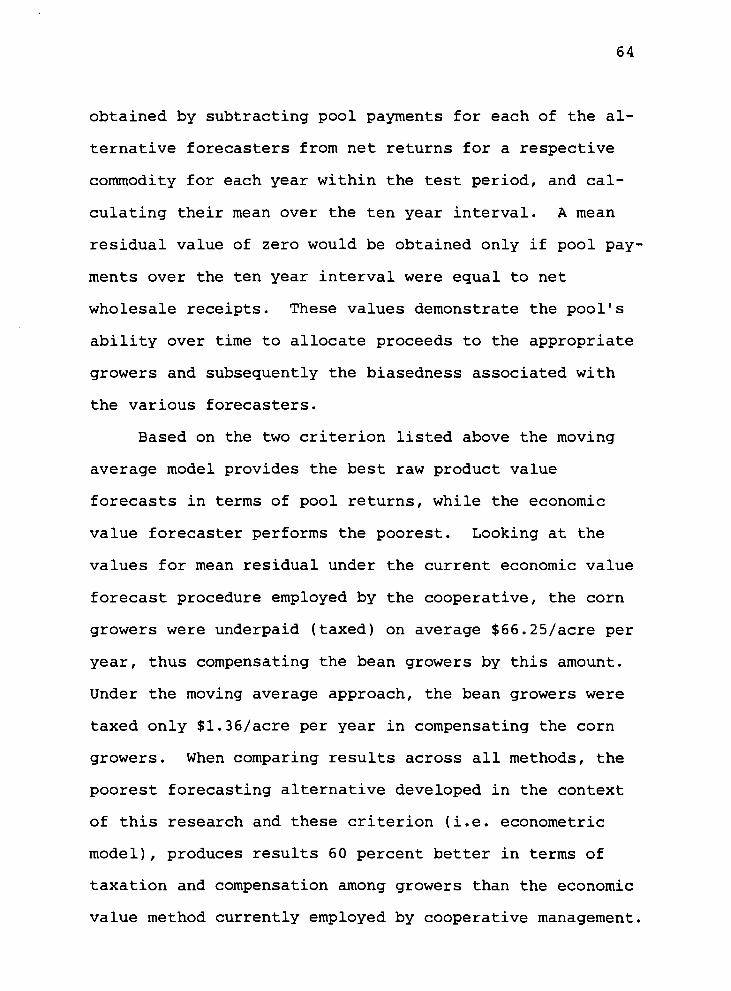
64
obtained by subtracting pool payments for each of the al-
ternative forecasters from net returns for a respective
commodity for each year within the test period, and cal-
culating their mean over the ten year interval. A mean
residual value of zero would be obtained only if pool pay-
ments over the ten year interval were equal to net
wholesale receipts. These values demonstrate the pool's
ability over time to allocate proceeds to the appropriate
growers and subsequently the biasedness associated with
the various forecasters.
Based on the two criterion listed above the moving
average model provides the best raw product value
forecasts in terms of pool returns, while the economic
value forecaster performs the poorest. Looking at the
values for mean residual under the current economic value
forecast procedure employed by the cooperative, the corn
growers were underpaid (taxed) on average $66.25/acre per
year, thus compensating the bean growers by this amount.
Under the moving average approach, the bean growers were
taxed only $1.36/acre per year in compensating the corn
growers. When comparing results across all methods, the
poorest forecasting alternative developed in the context
of this research and these criterion (i.e. econometric
model), produces results 60 percent better in terms of
taxation and compensation among growers than the economic
value method currently employed by cooperative management.
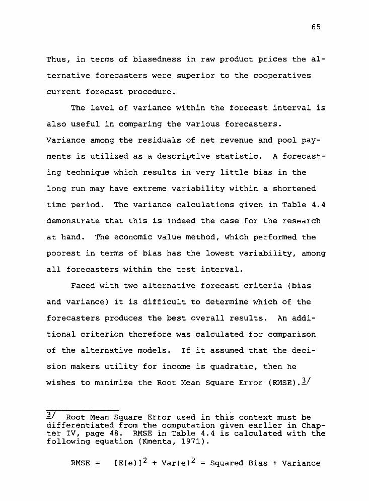
65
Thus, in terms of biasedness in raw product prices the al-
ternative forecasters were superior to the cooperatives
current forecast procedure.
The level of variance within the forecast interval is
also useful in comparing the various forecasters.
Variance among the residuals of net revenue and pool pay-
ments is utilized as a descriptive statistic. A forecast-
ing technique which results in very little bias in the
long run may have extreme variability within a shortened
time period. The variance calculations given in Table 4.4
demonstrate that this is indeed the case for the research
at hand. The economic value method, which performed the
poorest in terms of bias has the lowest variability, among
all forecasters within the test interval.
Faced with two alternative forecast criteria (bias
and variance) it is difficult to determine which of the
forecasters produces the best overall results. An addi-
tional criterion therefore was calculated for comparison
of the alternative models. If it assumed that the deci-
sion makers utility for income is quadratic, then he
wishes to minimize the Root Mean Square Error (RMSE).2/
±1 Root Mean Square Error used in this context must be differentiated from the computation given earlier in Chap- ter IV, page 48. RMSE in Table 4.4 is calculated with the following equation (Kmenta, 1971).
RMSE = [E(e)]2 + Var(e)2 = Squared Bias + Variance
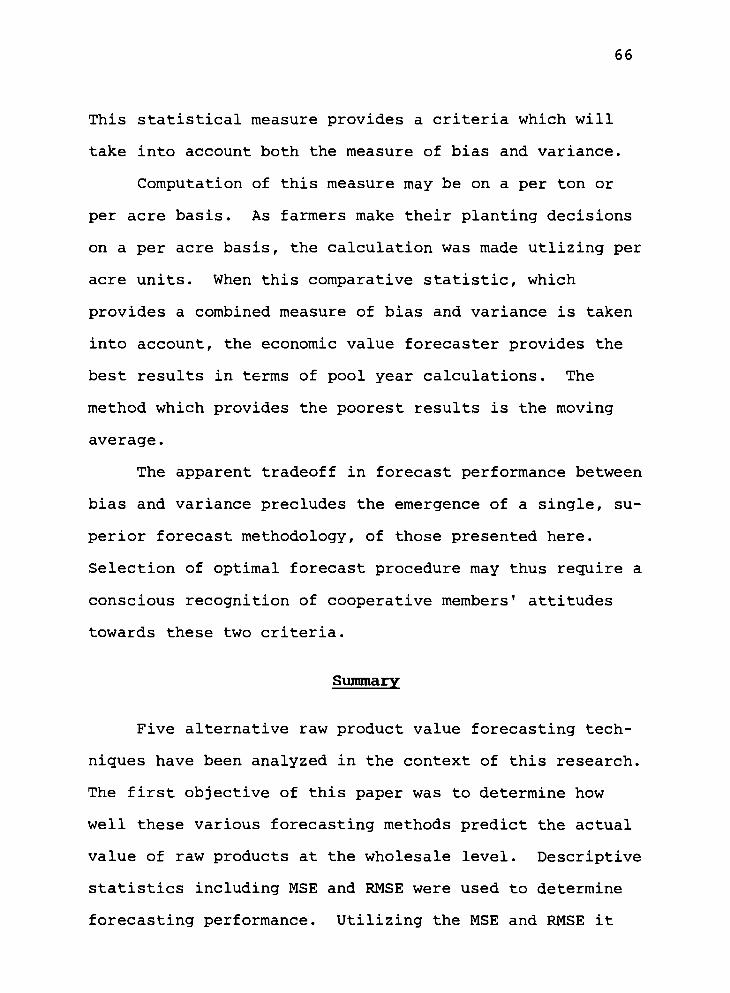
66
This statistical measure provides a criteria which will
take into account both the measure of bias and variance.
Computation of this measure may be on a per ton or
per acre basis. As farmers make their planting decisions
on a per acre basis, the calculation was made utlizing per
acre units. When this comparative statistic, which
provides a combined measure of bias and variance is taken
into account, the economic value forecaster provides the
best results in terms of pool year calculations. The
method which provides the poorest results is the moving
average.
The apparent tradeoff in forecast performance between
bias and variance precludes the emergence of a single, su-
perior forecast methodology, of those presented here.
Selection of optimal forecast procedure may thus require a
conscious recognition of cooperative members' attitudes
towards these two criteria.
Summary
Five alternative raw product value forecasting tech-
niques have been analyzed in the context of this research.
The first objective of this paper was to determine how
well these various forecasting methods predict the actual
value of raw products at the wholesale level. Descriptive
statistics including MSE and RMSE were used to determine
forecasting performance. Utilizing the MSE and RMSE it
67
was found that the three year moving average and exponen-
tial smoothing forecaster provide the best results when
taking both snap beans and sweet corn into consideration.
Graphical analysis was also used to track all five
forecasters over the ten year test period against the ac-
tual raw product value. No method in particular tracked
the actual raw product value consistently over the ten
year period. The econometric and composite forecasters
accounted for more turning points than the other methods,
while the exponential smoothing and moving average were
best able to follow general trends.
The second objective of this research was to deter-
mine the effects of the alternative forecasters on single
pool payments. The criteria used to evaluate pool pay-
ments were biasedness and variance. In terms of bias it
was shown that the moving average in particular as well as
the exponential smoothing techniques were far superior to
all others. When taking variance into account the
economic value provided the best results.
68
CHAPTER V
SUMMARY AND CONCLUSIONS
The objective of this research has been to explore
the performance of five alternative raw product valuation
procedures for a vertically integrated vegetable process-
ing and marketing cooperative. Four such alternative pro-
cedures were developed. These techniques, along with the
method currently employed by the cooperative, were then
used to calculate single-pool returns. The five proce-
dures were compared utilizing the comparative statistics
outlined in Chapter IV.
Assessment of Alternative Forecasting Methods
With Respect To Pool-Year Returns
Several criteria were used in assessing the alterna-
tive forecasting procedures and their effects on pool-year
returns. Comparative statistics (MSE and MAPE) were used
to measure how well individual forecasters predicted ac-
tual net returns per ton at the wholesale level of raw
products. These statistics revealed that the three-year
moving average generates the most accurate results when
taking both snap beans and sweet corn into consideration.
MSE and MAPE provide insight into how well individual
forecasters predict actual net returns per ton. However,
MSE and MAPE do not consider biasedness and variance in
69
reference to pool payments. Thus, additional criteria for
biasedness and variance must be taken into account for
pool-year returns. Biasedness between pool payments and
net returns is assumed to be the most important criteria
from the standpoint of grower members. Pool payment bias
in the context of this research is defined as the dif-
ference between mean net returns per ton and mean pool
payments per ton. Stated alternatively, it is the dif-
ference between what growers received for their raw
products and the net revenues the raw products earned at
the wholesale level. The three-year moving average
forecaster provided the least biased payment while the
econometric model method provided the most biased pay-
ments. Payment variance is a measure of the dispersion of
the deviation of pool payments around their mean value.
The cooperative's present method of setting economic
values resulted in the lowest payment variance, over the
ten-year test horizon of any of the methods studied.
Forecasting Methods
Econometric Models
The econometric models for both snap beans and sweet
corn performed poorly over the ten period forecast inter-
val. These models provided the highest measure of bias of
any forecaster. The poor forecasts provided by the
70
econometric models may have been caused by the absence of
firm-specific explanatory variables. Inclusion of a firm-
specific variable, for example to account for the rapid
expansion of cooperative size in 1980, may have improved
forecast performance.
In a later application, the econometric models were
fitted to post-1979 data, with subsequent forecasts over
the 1983-85 time interval. The adjusted R2s for the
forecasts made over the three-year test horizon were near
0.90. The results provided by this limited data set sug-
gest the importance of the forecast horizon. Providing
there are no further near-term structural changes within
the Willamette Valley vegetable processing industry, the
econometric models may generate better results in the fu-
ture than those evidenced over the 1975-86 test period.
Naive Forecasters
Results generated by the single-variable forecasting
techniques (i.e. three-year moving average and exponential
smoothing) suggest that under certain conditions these
forecasters perform quite well. The univariate methods
are useful in accounting for random shocks in net returns
per ton. On the other hand, if these random shocks are
turning points of great magnitude, the univariate
forecasters tend to perform quite poorly. This shortcom-
ing of the univariate forecasters cannot be avoided due to
71
the inherent nature of their forecasting process. Thus,
these forecasting methods are most appropriate for data
with gradually changing means.
Composite Forecaster
The composite forecaster is dependent upon the
ability of all forecasters and the weighting scheme used
to generate the forecast. Once the weighting scheme is
chosen, performance of the composite is dictated by the
performance of other methods. The limitation was not in
the weight chosen, but in the random performance of the
alternative forecasters. Individually, all forecasters
performed well at one point in time or another. If an in-
dividual technique was providing good results, a large
weight would be assigned to that particular forecaster for
the next period. Oftentimes a method with large assigned
weight would perform poorly in the subsequent period. In
that case, the composite forecast for the following time
period would also perform poorly.
Applications for Single-Pool Cooperatives
Application of the research findings in this paper
are dependent on cooperatives' notions of equity (measure
of bias) and dispersion of pool-payments around their mean
values (measure of variance). For example, equity may be
the foremost concern, with the criterion being that the
72
long run average pool payments to each member be equal to
each member's products average contribution to total pool
returns. If this is the criterion sought, then the three-
year moving average and double exponential smoothing tech-
niques provide the most desirable results, clearly outper-
forming the other methods. On the other hand, the
cooperative's present method of selecting economic values
provides the best results if variance (minimum variation
in values over time) is the most important criterion. The
economic value method also would provide the best results
if variance and bias were were thought of as equal in im-
portance. Thus, applications to processing cooperatives
may vary depending on members' perceived importance of
various criteria used in evaluation of pool payments.
Some of the alternative forecasting procedures
developed in the context of this research did perform
quite well, paticularily in terms of biasedness. From the
grower-member standpoint it is a reasonable presumption
that bias is of greater concern than variance. If bias
and variance are not thought of as equal in importance,
then cooperative management may wish to incorporate one or
more of the methods developed in this research in estab-
lishing raw product price. The tendency towards bias and
improper price signals in the raw product market are in-
terrelated. The relationship between improper price sig-
nals and bias is inherent in the cooperative's calculation
73
of payments to growers. Raw product forecasts are the
basis for payment to growers as shown in equation 2.2.
Adoption of one or more of the alternative forecasters
would help alleviate problems of disequilibrium between
the raw product and finished product markets. Further-
more, decreased bias would help remedy the long run taxa-
tion of some growers and the subsidization of others.
Limitations
The cooperative upon which this research is based
handles a number of different fruits and vegetables.
Revenues from all commodities are grouped into a single-
pool. Allocation of these revenues to individual com-
modities is then derived utilizing equations 2.1 and 2.2.
In this paper, a simplified representation of the coopera-
tive was adopted. Calculation of single-pool returns was
based upon the methods currently employed by cooperative
management. However, only two commodities, snap beans and
sweet corn, were included in the modeled pool. Inclusion
of more than two commodities would have given a more
reasonable representation of the risk-return tradeoff of a
single pool and the resulting allocation of revenues to
individual commodities.
The two-commodity single pool modeled in the context
of this research is justified by the research objectives
given in Chapter I. If the research objective had been
74
solely to measure payment variance, then a two-commodity
single pool indeed would have been a serious limitation.
The main objective of this research, however, was to
assess deviation of members' payments from members' con-
tribution to pool returns. The two commoditites included
in this research comprise a major portion of the
cooperative's single pool in terms of economic value.
Snap beans and sweet corn encompass up to 80 percent of
total economic values assigned to all commodities. Thus,
in constructing a pool with only two commodities it is
evident snap beans and sweet corn were the appropriate
choice. Furthermore, the theory which dictates the use of
single pools is not dependent on the number of commodities
within the pool but the methods used to allocate revenues
among growers of different products.
Suggestions for Further Research
The structure of the processed vegetable market in
the Northwest Region has undergone extensive change in
recent years. Not only has the industry changed, but the
firms within the market have changed in both size and
operational characteristics. Forecasting models which
utilize explanatory variables based on national data can-
not completely and accurately reflect changes within these
firms. Further research could attempt to incorporate ex-
planatory variables which are firm-specific in nature.

75
Inclusion of explanatory variables such as fruit or
vegetable packed in the Northwest, purchase orders or
bookings for final products, or firm-specific stocks might
enhance the forecasting ability of an econometric model.
76
BIBLIOGRAPHY
Anderson, J., R. Dillon, and B. Hardaker. Agricultural Decision Analysis. Ames, Iowa: Iowa State University Press, 1977.
Bessler, D.A. and J.A. Brandt. "Composite Forecasting of Livestock Prices: An Analysis of Combining Alterna- tive Forecasting Methods." Department of Agricultural Economics, Agricultural Experiment Station Bulletin No. 265, Purdue University, West Lafayette, December 1979.
Buccola, S.T. and A. Subaei. "Optimal Market Pools for Agricultural Cooperatives." American Journal of Agricultural Economics, 63(1985):70-79.
The Council of Economic Advisors. "Economic Indicators." Prepared for the Joint Economic Committee, 1959-1986.
Edward E. Judge and Sons, Inc. The Almanac of Canning, Freezing, and Preserving Industries. 1959-1986.
Foote, R.J. Analytical Tools for Studying Demand and Price Structures. United States Department of Agriculture, Agricultural Handbook No. 146, Washington, D.C., 1958.
Garoyan, L. "Developments in the Theory of Farmer Cooperatives." American Journal of Agricultural Economics, 65(1983):1096-1098.
Gujarati, D. Basic Econometrics. McGraw-Hill Book Com- pany, New York, New York, 1978.
Knoeber, C.R. and D.L. Baumer. "Understanding Retained Patronage Refunds in Agricultural Cooperatives." American Journal of Agricultural Economics, 65(1983):30-37.
Kmenta, J. Elements of Econometrics. New York: Macmil- lan Publishing Co., Inc. 1971.
Kuznets, G.M. "Forecasting F.O. B. Prices of California Canned Tomato Products." A Cooperative Commodity Transfer Pricing Study; Toche, Ross and Company, Sep- tember 1982.
Makridakis, S. and S. Wheelwright. Interactive Forecast- ing, Univariate and Multivariate Methods. Second edi- tion, San Francisco, California: Holden-Day, Inc., 1978.
77
McGuigan, J. and C. Moyer. Managerial Economics. Fourth Edition, San Francisco, California: West Publishing Company, 1986.
Miles, S.D. Unpublished data. Extension Economic Infor- mation Service, Oregon State University, Corvallis. 1960-1985.
Pindyck, R. and D. Rubinfield. Econometric Models and Economic Forecasts. Second edition. New York, New York: McGraw-Hill Book Comapny, 1976.
Rao, P. and R. Miller. Applied Econometrics. Belmont, California: Wadsworth Publishing Company, 1971.
Roy, E.P. Cooperatives: Development, Principles and Management. Third Edition, Daniville, Illinois: The Interestate Press, 1976.
Smith, J. Interviews. Corporate Planning Director, Agricultural Processing and Marketing Cooperative. 1984.
Snedecor, G. and W. Cochran. Statistical Methods. Seventh edition, Ames, Iowa: Iowa State University Press, 1980.
Subaei, A.M.A. "Alternative Market Pools for Agricultural Cooperatives: A Decision Analysis Framework," Un- published Ph.D. dissertation, Oregon State University, 1984.
Tomek, W. and K. Robinson. Agricultural Product Prices, 2nd edition. Ithaca, NY: Cornell University Press, 1982.
United States Department of Agriculture, Statistical Reporting Service, Crop Reporting Board. "Summary of Regional Cold Storage Holdings". Various years.
Wiese, M.A. "Alternative Methods of Raw Product Valuation for Agricultural Cooperatives: A Forecasting Ap- proach," Unpublished M.S. thesis, Oregon State Univer- sity, 1986.

APPENDICES
78
APPENDIX A
POOL-YEAR RETURNS AND COMPARATIVE STATISTICS
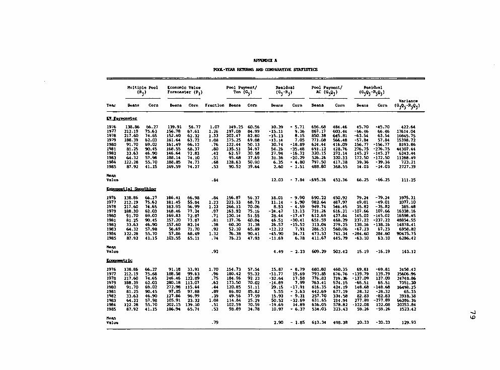
AFPEHDLI A
FOOL-YEAR RETURNS AHD COMPARATIVE STATISTICS
Multiple Pool Economic Value Pool Payment/ Residual Pool Payment/ Residual (Rj) Forecaster (Pj) Ton (Gj) <Gr Rj) AC (GJQJ) WjQy -w
Variance Year Beans Corn Beans Com Fraction Beans Com Beans Com Beans Com Beans Com J0JQj-W
EV_EaX£C££££
1976 138.86 66.27 139.91 56.77 1.07 149.25 60.56 10.39 - 5.71 656.68 484.46 45.70 -45.70 422.64 1977 212.19 75.63 156.78 67.61 1.26 197.08 84.99 -15.11 9.36 867.17 603.44 -66.46 66.46 17614.04 1978 217.60 74.65 152.40 62.32 1.33 202.47 82.80 -15.13 8.15 850.38 645.Bl -63.54 63.54 16845.75 1979 188.39 62.03 161.64 63.72 1.08 175.25 69.08 -13.14 7.05 771.08 566.48 -57.84 57.84 15398.72 1980 91.70 69.02 161.49 66.12 .76 122.44 50.13 30.74 -18.89 624.44 416.09 156.77 -156.77 8193.86 1981 81.25 90.45 168.55 68.37 .80 135.51 54.97 54.26 -35.48 691.12 428.76 276.75 -276.75 44307.44 1982 33.63 46.90 146.64 72.83 .42 62.57 30.58 27.94 -16.32 320.15 272.14 145.27 -145.27 6243.44 1983 64.32 57.98 188.14 74.10 .51 95.68 37.69 31.36 -20.29 526.26 320.33 172.50 -172.50 11288.49 1984 122.28 55.70 188.85 74.73 .68 128.63 50.90 6.35 - 4.80 797.50 417.38 39.36 -39.36 723.21 1985 87.92 41.15 169.59 74.27 .53 90.52 39.64 2.60 - 1.51 488.80 368.55 14.03 -14.03 2727.39
Mean Value .84 12.03 - 7.84 •695.36 452.36 66.25 -66.25 111.25
Emoneotlal Snoothlng
1976 138.86 66.27 186.41 66.98 .84 156.87 56.37 18.01 - 9.90 690.22 450.92 79.24 -79.24 3975.31 1977 212.19 75.63 181.45 55.84 1.23 223.33 68.73 11.14 - 6.90 982.64 487.97 49.01 -49.01 1077.10 1978 217.60 74.65 183.95 56.99 1.23 266.13 70.06 8.53 - 4.59 949.74 546.45 35.82 -35.82 385.48 1979 188.30 62.03 168.46 77.24 .97 163.92 75.16 -24.47 13.13 721.26 616.31 -107.66 107.66 16338.16 1980 91.70 69.02 169.83 72.87 .71 120.14 51.55 28.44 -17.47 612.69 427.84 145.02 -145.02 16598.45 1981 81.25 90.45 157.20 73.87 .81 127.76 60.04 46.51 -30.41 651.59 468.29 237.22 -237.22 48854.55 1982 33.63 46.90 157.60 82.14 .38 60.20 31.38 26.57 -15.52 313.04 279.25 138.16 -138.16 14878.41 1983 64.32 57.98 56.69 71.70 .92 52.10 65.89 -12.22 7.91 286.53 560.06 -67.23 67.23 6958.82 1984 122.28 55.70 57.86 68.49 1.32 76.38 90.41 -45.90 34.71 473.53 741.34 -284.60 284.60 90475.75 1985 87.92 41.15 103.55 65.11 .74 76.23 47.93 -11.69 6.78 411.67 445.79 -63.10 63.10 6286.42
Mean Value .92 4.49 - 2.23 609.29 502.42 15.19 -16.19 143.12
Eooooewtric
1976 138.86 66.27 91.18 33.91 1.70 154.73 57.54 15.87 - 8.79 680.80 460.35 69.81 -69.81 2458.42 1977 212.19 75.68 1B8.58 99.63 .96 180.42 95.32 -31.77 19.69 793.85 676.76 -139.79 139.79 25606.96 1978 217.60 74.65 246.46 122.89 .75 184.96 92.23 -32.64 17.58 776.83 719.36 -137.09 137.09 24748.86 1979 188.39 62.03 280.18 113.07 .62 173.50 70.02 -14.89 7.99 763.41 574.15 -65.51 65.51 7351.30 1980 91.70 69.02 272.98 115.44 .44 120.85 51.11 29.15 -17.91 616.35 424.19 148.68 -148.68 16498.25 1981 81.25 90.45 97.85 97.88 .89 86.80 85.82 5.55 - 3.63 442.69 677.19 28.32 -28.32 65.35 1982 33.63 46.90 127.86 96.99 .39 49.56 37.59 15.93 - 9.31 257.70 334.58 62.83 -82.83 3918.38 1983 64.32 57.98 105.91 23.32 1.08 114.84 25.29 50.52 -32.69 631.65 214.94 277.89 -277.89 66386.36 1984 122.28 55.70 202.15 139.10 .51 102.59 70.59 -19.69 14.89 636.05 578.82 -122.08 122.08 20253.84 1985 87.92 41.15 186.94 65.74 .53 98.B9 34.78 10.97 - 6.37 534.03 323.43 59.26 -59.26 1523.42
Mean Value .79 2.90 - 1.85 613.34 498.38 20.23 -20.23 129.93
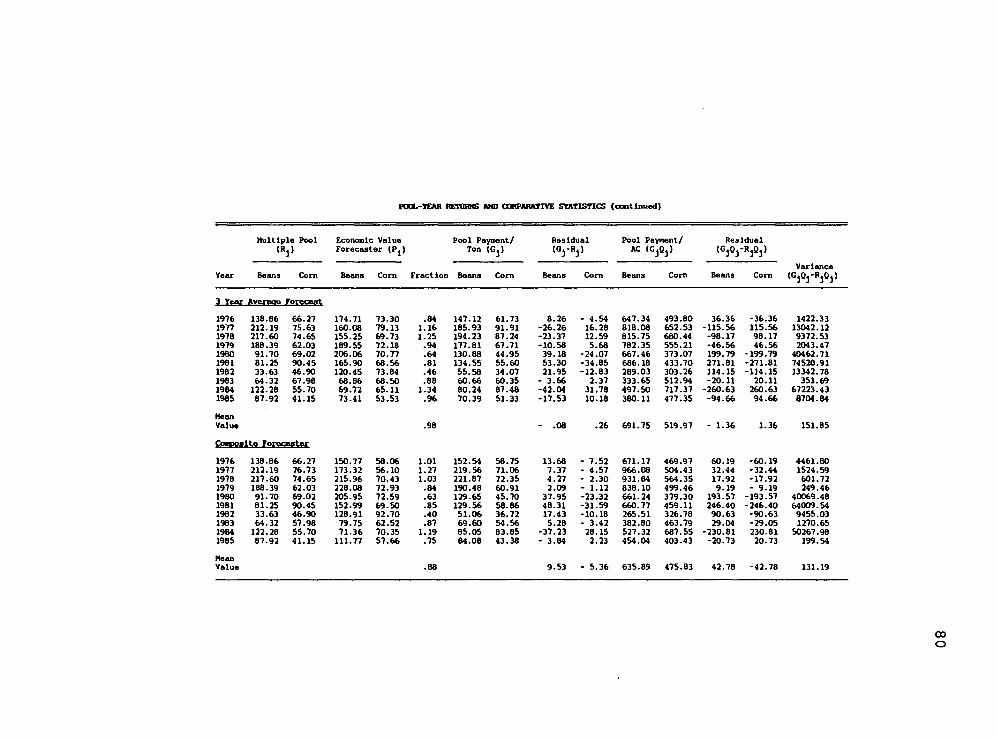
POOL-TEAH RETOKje AND OOHPARATIVE STATISTICS (oontlnued)
Multiple Pool Econotolc Value Pool Payment/ Residual Pool Payment/ Residual (R 3> Forecaster (Pj) Ton (Gj) (O^-l V AC (G^) (OjQy -w
Variance Year Beans Com Beans Com Fraction Com Beans Com Beans Com Beans Com (GjQj-RjQj)
? Tw ^ygrwo rorwtt
1976 138.86 66.27 174.71 73.30 .84 147.12 61.73 6.26 - 4.54 647.34 493.80 36.36 -36.36 1422.33 19T7 212.19 75.63 160.08 79.13 1.16 185.93 91.91 -26.26 16.28 818.08 652.53 -115.56 115.56 13042.12 197B 217.60 74.65 155.25 69.73 1.25 194.23 87.24 -23.37 12.59 815.75 680.44 -98.17 98.17 9372.53 1979 188.39 62.03 189.55 72.18 .94 177.81 67.71 -10.58 5.68 782.35 555.21 -46.56 46.56 2043.47 1980 91.70 69.02 206.06 70.77 .64 130.88 44.95 39.18 -24.07 667.46 373.07 199.79 -199.79 40462.71 1981 81.25 90.45 165.90 68.56 .81 134.55 55.60 53.30 -34.85 686.18 433.70 271.81 -271.81 74520.91 1982 33.63 46.90 120.45 73.84 .46 55.58 34.07 21.95 -12.83 289.03 303.26 114.15 -114.15 13342.78 1983 64.32 67.98 68.86 68.50 .88 60.66 60.35 - 3.66 2.37 333.65 512.94 -20.11 20.11 351.69 1984 122.28 55.70 69.72 65.11 1.34 80.24 87.48 -42.04 31.78 497.50 717.37 -260.63 260.63 67223.43 198S 87.92 41.15 73.41 53.53 .96 70.39 51.33 -17.53 10.18 380.11 477.35 -94.66 94.66 8704.84
Mean Value .98 - .08 .26 691.75 519.97 - 1.36 1.36 151.85
Caeoalte Forecastor
1976 138.86 66.27 150.77 58.06 1.01 152.54 58.75 13.68 - 7.52 671.17 469.97 60.19 -60.19 4461.80 1977 212.19 76.73 173.32 56.10 1.27 219.56 71.06 7.37 - 4.57 966.08 504.43 32.44 -32.44 1524.59 1978 217.60 74.65 215.96 70.43 1.03 221.87 72.35 4.27 - 2.30 931.84 564.35 17.92 -17.92 601.72 1979 188.39 62.03 228.08 72.93 .84 190.48 60.91 2.09 - 1.12 838.10 499.46 9.19 - 9.19 249.46 1980 91.70 69.02 205.95 72.59 .63 129.65 45.70 37.95 -23.32 661.24 379.30 193.57 -193.57 40069.48 1981 81.25 90.45 152.99 69.50 .85 129.56 58.86 48.31 -31.59 660.77 459.11 246.40 -246.40 64009.54 1982 33.63 46.90 128.91 92.70 .40 51.06 36.72 17.43 -10.18 265.51 326.78 90.63 -90.63 9455.03 1983 64.32 57.98 79.75 62.52 .87 69.60 54.56 5.28 - 3.42 382.80 463.79 29.04 -29.05 1270.65 1984 122.28 55.70 71.36 70.35 1.19 85.05 83.85 -37.23 28.15 527.32 687.55 -230.81 230.81 50267.98 1985 87.92 41.15 111.77 57.66 .75 84.08 43.38 - 3.84 2.23 454.04 403.43 -20.73 20.73 199.54
Mean Value .88 9.53 - 5.36 635.89 475.83 42.78 -42.78 131.19
00 o
81
APPENDIX B
ECONOMETRIC MODEL ESTIMATION RESULTS
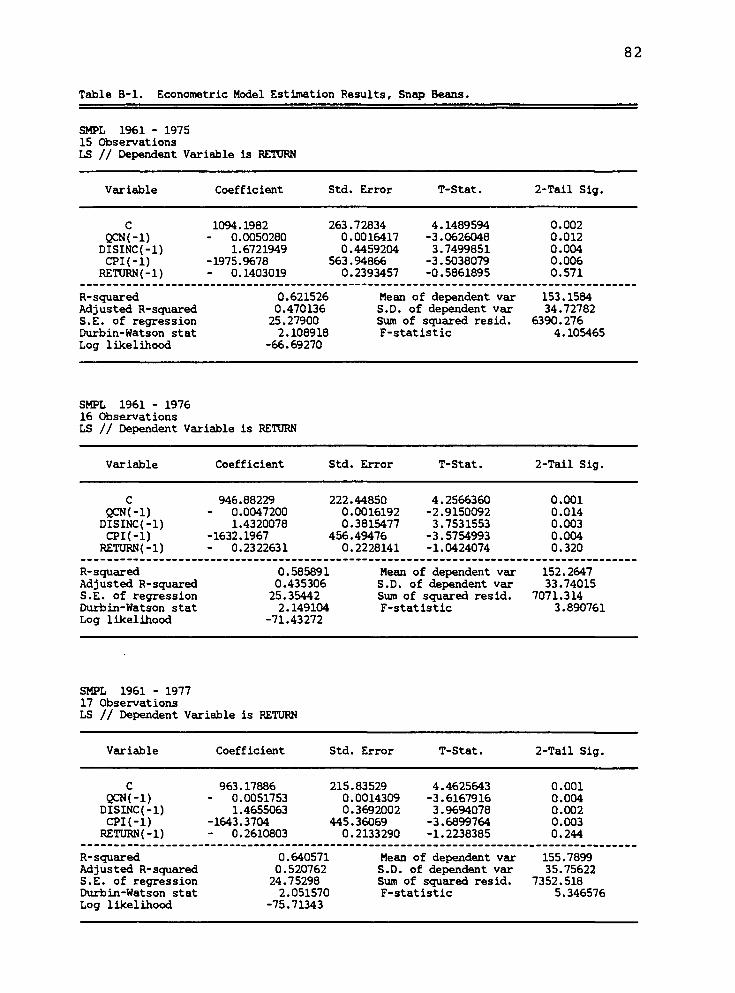
82
Table B-1. Econometric Model Estimation Results, Snap Beans.
SMPL 1961 - 1975 15 Observations LS // Dependent Variable is RETURN
Variable Coefficient Std. Error T-Stat. 2-Tail Sig.
C QCN(-l)
DISINC(-l) CPI(-l)
RETURN(-l)
1094.1982 - 0.0050280
1.6721949 -1975.9678 - 0.1403019
263.72834 0.0016417 0.4459204
563.94866 0.2393457
4.1489594 -3.0626048 3.7499851
-3.5038079 -0.5861895
0.002 0.012 0.004 0.006 0.571
R-squared Adjusted R-squared S.E. of regression Durbin-Watson stat Log likelihood
0. 0.^
25. 2.
-66.
621526 470136 27900 ,108918 69270
i Mean of dependent var S.D. of dependent var Sum of squared resid.
I F-statistic
153.1584 34.72782
6390.276 4.105465
SMPL 1961 - 1976 16 Observations LS // Dependent Variable is RETURN
Variable Coefficient Std. Error T-Stat. 2-Tail Sig.
c 946.88229 222.44850 4.2566360 0.001 QCN(-l) - 0.0047200 0.0016192 -2.9150092 0.014
DISINC(-l) 1.4320078 0.3815477 3.7531553 0.003 CPI(-l) -1632.1967 456.49476 -3.5754993 0.004
RETURNf-l) - 0.2322631 0.2228141 -1.0424074 0.320
R-squared 0.585891 Mean of dependent var 152.2647 Adjusted R-squared 0.435306 S.D. of dependent var 33.74015 S.E. of regression 25.35442 Sum of squared resid. 7071.314 Durbin-Watson stat 2.149104 F-statistic 3.890761 Log likelihood -71.43272
SMPL 1961 - 1977 17 Observations LS // Dependent Variable is RETURN
Variable Coefficient Std. Error T-Stat. 2-Tail Sig.
C 963.17886 215.83529 4.4625643 0.001 QCN(-l) - 0.0051753 0.0014309 -3.6167916 0.004
DISINC(-l) 1.4655063 0.3692002 3.9694078 0.002 CPI(-l) -1643.3704 145.36069 -3.6899764 0.003 RETURN(-l) - 0.2610803 0.2133290 -1.2238385 0.244
R-squared 0.640571 Mean of dependent var 155.7899 Adjusted R-squared 0.520762 S.D. of dependent var 35.75622 S.E. of regression 24.75298 Sum of squared resid. 7352.518 Durbin-Watson stat 2.051570 F-statistic 5.346576 Log likelihood -75.71343
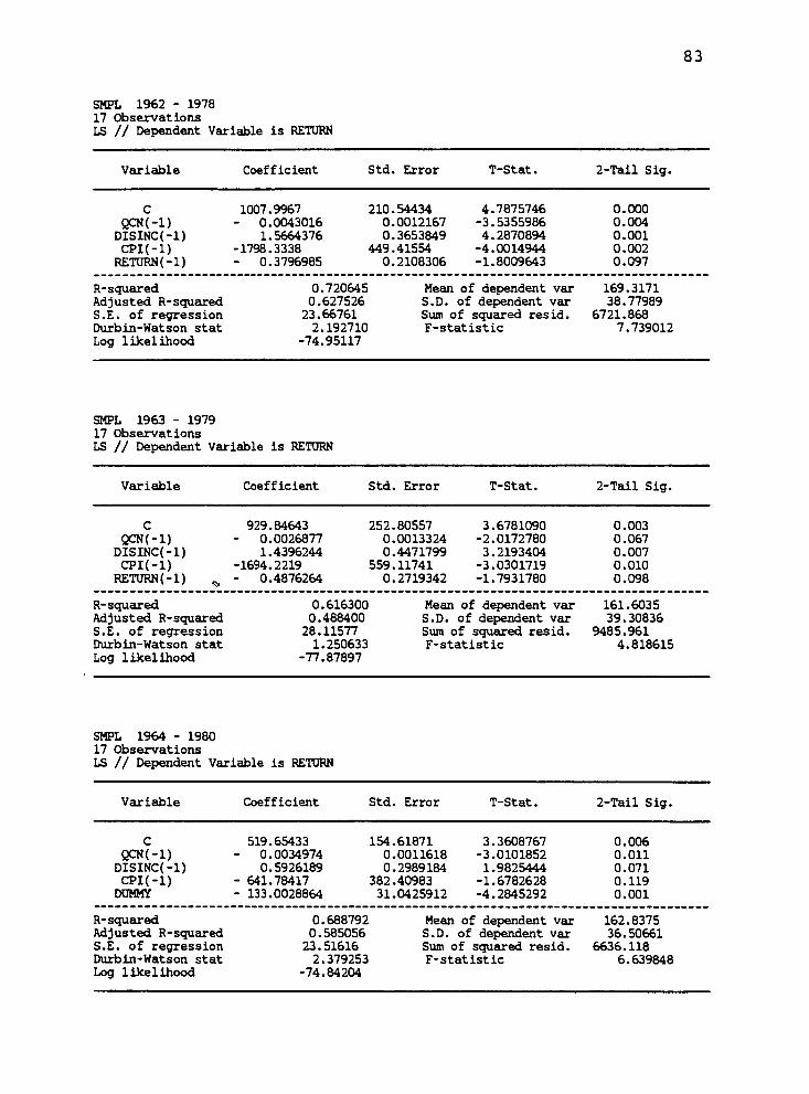
83
SMPL 1962 - 1978 17 Observations LS // Dependent Variable is RETURN
Variable Coefficient Std. Error T-Stat. 2-Tail Sig.
C QCN(-l) DISINC(-l) CPI(-l) RETURN(-l)
1007.9967 - 0.0043016
1.5664376 -1798.3338 - 0.3796985
210.54434 0.0012167 0.3653849
449.41554 0.2108306
4.7875746 -3.5355986 4.2870894 -4.0014944 -1.8009643
0.000 0.004 0.001 0.002 0.097
R-squared Adjusted R-squared S.E. of regression Durbin-Watson stat Log likelihood
0.720645 0.627526 23.66761 2.192710
-74.95117
i Mean of dependent S.D. of dependent Sum of squared res
I F-statistic
var var id.
169.3171 38.77989
6721.868 7.739012
SMPL 1963 - 1979 17 Observations LS // Dependent Variable is RETURN
Variable Coefficient Std. Error T-Stat. 2-Tail Sig.
C QCN(-l) DISINC(-l) CPI(-l) RETURN(-l)
929.84643 ■ 0.0026877
1.4396244 -1694.2219 - 0.4876264
252.80557 0.0013324 0.4471799
559.11741 0.2719342
3.6781090 -2.0172780 3.2193404 -3.0301719 -1.7931780
0.003 0.067 0.007 0.010 0.098
R-squared 0.616300 Mean of dependent var 161.6035 Adjusted R-squared 0.488400 S.D. of dependent var 39.30836 S.E. of regression 28.11577 Sum of squared resid. 9485.961 Durbin-Watson stat 1.250633 F-statistic 4.818615 Log likelihood -77.87897
SMPL 1964 - 1980 17 Observations LS // Dependent Variable is RETURN
Variable Coefficient Std. Error T-Stat. 2-Tail Sig.
c 519. ,65433 154. .61871 3.3608767 0.006 QCN(-l) - 0. .0034974 0. .0011618 -3.0101852 0.011 DISINC(-l) 0, .5926189 0, .2989184 1.9825444 0.071 CPI(-l) - 641. .78417 382, .40983 -1.6782628 0.119 DUMMY - 133, .0028864 31. .0425912 -4.2845292 0.001
R-squared 0.688792 Mean of dependent var 162.8375 Adjusted R-squared 0.585056 S.D. of dependent var 36.50661 S.E. of regression 23.51616 Sum of squared resid. 6636.118 Durbin-Watson stat 2.379253 F-statistic 6.639848 Log likelihood -74.84204
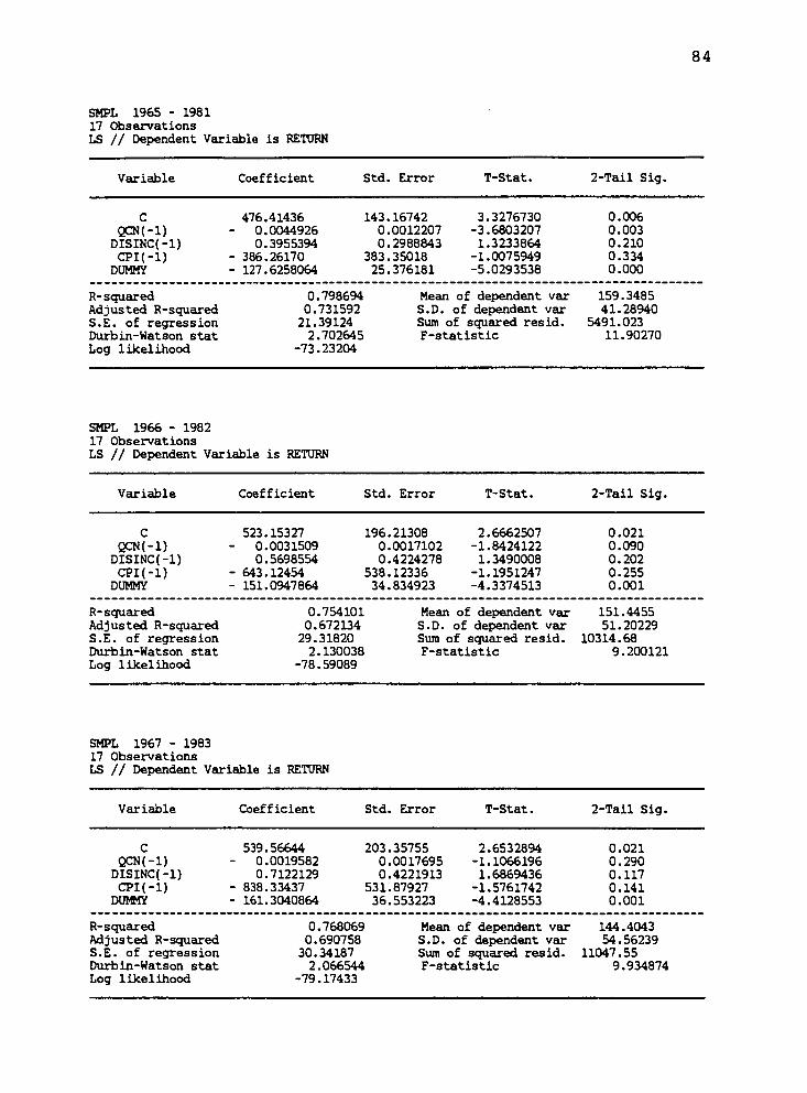
SMPL 1965 - 1981 17 Observations LS // Dependent Variable is RETURN
84
Variable Coefficient Std. Error T-Stat. 2-Tail Sig.
c 476.41436 143.16742 3.3276730 0.006 QCN(-l) - 0.0044926 0.0012207 -3.6803207 0.003
DISINC(-l) 0.3955394 0.2988843 1.3233864 0.210 CPI(-l) - 386.26170 383.35018 -1.0075949 0.334
DUMMY - 127.6258064 25.376181 -5.0293538 0.000
R-squared 0.798694 Mean of dependent var 159.3485 Adjusted R-squared 0.731592 S.D. of dependent var 41.28940 S.E. of regression 21.39124 Sura of squared resid. 5491.023 Durbin-Watson stat 2.702645 F-statistic 11.90270 Log likelihood -73.23204
SMPL 1966 - 1982 17 Observations LS // Dependent Variable is RETURN
Variable Coefficient Std. Error T-Stat. 2-Tail Sig.
c 523.15327 196.21308 2.6662507 0.021 QCN(-l) - 0.0031509 0.0017102 -1.8424122 0.090
DISINC(-l) 0.5698554 0.4224278 1.3490008 0.202 CPI(-l) - 643.12454 538.12336 -1.1951247 0.255
DUMMY - 151.0947864 34.834923 -4.3374513 0.001
R-squared 0.754101 Mean of dependent var 151.4455 Adjusted R-squared 0.672134 S.D. of dependent var 51.20229 S.E. of regression 29.31820 Sum of squared resid. 10314.68 Durbin-Watson stat 2.130038 F-statistic 9.200121 Log likelihood -78.59089
SMPL 1967 - 1983 17 Observations LS // Dependent Variable is RETURN
Variable Coefficient Std. Error T-Stat. 2-Tail Sig.
C QCN(-l)
DISINC(-l) CPI(-l) DUMMY
539.56644 - 0.0019582
0.7122129 - 838.33437 - 161.3040864
203.35755 0.0017695 0.4221913
531.87927 36.553223
2.6532894 -1.1066196 1.6869436
-1.5761742 -4.4128553
0.021 0.290 0.117 0.141 0.001
R-squared Adjusted R-squared S.E. of regression Durbin-Watson stat Log likelihood
0. 0.'
30. 2.
-79.
768069 690758 34187 066544 17433
> Mean of dependent S.D. of dependent ' Sura of squared res F-statistic
var var id.
144.4043 54.56239
11047.55 9.934874
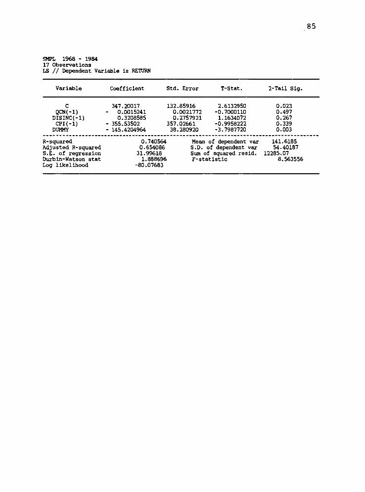
SMPL 1968 - 1984 17 Observations IS II Dependent Variable is RETURN
85
Variable Coefficient Std. Error T-Stat. 2-Tail Sig.
c 347.20017 132.85916 2.6132950 0.023 QCN(-l) - 0.0015241 0.0021772 -0.7000110 0.497
DISINC(-l) 0.3208585 0.2757921 1.1634072 0.267 CPI(-l) - 355.53502 357.02661 -0.9958222 0.339 DUMMY - 145.4204964 38.280920 -3.7987720 0.003
R-squared 0.740564 Mean of dependent var 141.6185 Adjusted R-squared 0.654086 S.D. of dependent var 54.40187 S.E. of regression 31.99618 Sum of squared resid. 12285.07 Durbin-Watson stat 1.888696 F-statistic 8.563556 Log likelihood -80.07683
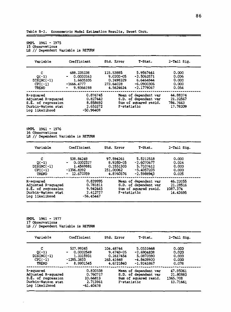
Table B-2. Econometric Model Estimation Results, Sweet Com.
SMPL 1961 - 1975 15 Observations LS // Dependent Variable is RETURN
86
Variable Coefficient Std. Error T-Stat. 2-Tail Sig.
c 688.235238 115.53885 5.9567441 0.000 Q(-l) - 0.0003163 9.020D-05 -3.5062571 0.006
DISINC(-l) 1.6605105 0.2498329 6.6464844 0.000 CPI(-l) -1666.4777 273.64028 -6.0900306 0.000 TREND - 9.9366198 4.5624634 -2.1779067 0.054
R-squared 0.876745 Mean of dependent var 44.88374 Adjusted R-squared 0.827442 S.D. of dependent var 21.32567 S.E. of regression 8.858692 Sum of squared resid. 784.7643 Durbin-Watson stat 2.653372 F-statistic 17.78309 Log likelihood -50.96408
SMPL 1961 - 1976 16 Observations LS // Dependent Variable is RETURN
Variable Coefficient Std. Error T-Stat. 2-Tail Sig.
c 538.84249 97.594261 5.5212518 0.000 Q(-l) - 0.0002327 8.928D-05 -2.6070677 0.024
DISINC(-l) 1.4569881 0.2551303 5.7107612 0.000 CPI(-l) -1356.8392 251.00062 -5.4057205 0.000 TREND - 12.672359 4.8760576 -2.5988943 0.025
R-squared 0.839995 Mean of dependent var 46.22055 Adjusted R-squared 0.781811 S.D. of dependent var 21.28516 S.E. of regression 9.942443 Sum of squared resid. 1087.374 Durbin-Watson stat 2.412727 F-statistic 14.43695 Log likelihood -56.45447
SMPL 1961 - 1977 17 Observations LS // Dependent Variable is RETURN
Variable Coefficient Std. Error T-Stat. 2-Tail Sig.
C 527.99245 104.48744 5.0531668 0.000 Q(-l) - 0.0002549 9.474D-05 -2.6904838 0.020
DISINC(-l) 1.3315931 0.2617454 5.0873590 0.000 CPI(-l) -1285.3833 265.41648 -4.8428920 0.000 TREND - 8.9901545 4.6721840 -1.9241867 0.078
R-squared 0.820538 Mean of dependent var 47.95061 Adjusted R-squared 0.760717 S.D. of dependent var 21.80883 S.E. of regression 10.66813 Sum of squared resid. 1365.708 Durbin-Watson stat 2.713961 F-statistic 13.71661 Log likelihood -61.40478
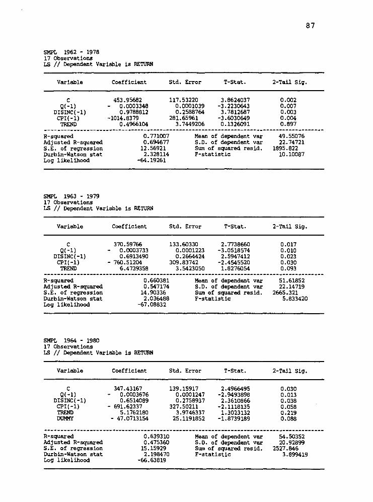
87
SMPL 1962 - 1978 17 Observations LS // Dependent Variable is RETURN
Variable Coefficient Std. Error T-Stat. 2-Tail Sig.
C Q(-l)
DISINC(-l) CPI(-l) TREND
453.95682 - 0.0003348
0.9788812 -1014.8379
0.4966104
117,53220 0,0001039 0,2588764
281.65961 3.7449206
3.8624037 -3.2230643 3.7812687 -3.6030649 0.1326091
0.002 0.007 0.003 0.004 0.897
R-squared Adjusted R-squared S.E. of regression Durbin-Watson stat Log likelihood
0. 0.
12. 2.
-64.
771007 694677 56921 328114 19261
Mean of dependent S.D. of dependent Sum of squared res F-statistic
var var lid.
49.55076 22.74721
1895.822 10.10087
SMPL 1963 - 1979 17 Observations LS // Dependent Variable is RETURN
Variable Coefficient Std. Error T-Stat. 2-Tail Sig.
c 370.59766 133.60330 2.7738660 0.017 Q(-l) - 0.0003733 0.0001223 -3.0518574 0.010
DISINC(-l) 0.6913490 0.2664424 2.5947412 0.023 CPI(-l) - 760.51204 309.83742 -2.4545520 0.030 TREND 6.4739358 3.5423050 1.8276054 0.093
R-squared 0.660381 Mean of dependent var 51.61852 Adjusted R-squared 0.547174 S.D. of dependent var 22.14719 S.E. of regression 14.90336 Sum of squared resid. 2665.321 Durbin-Watson stat 2.036488 F-statistic 5.833420 Log likelihood -67.08832
SMPL 1964 - 1980 17 Observations LS // Dependent Variable is RETURN
Variable Coefficient Std. Error T-Stat. 2-Tail Sig.
c 347.43167 L39.15917 2.4966495 0.030 Q(-l) - 0.0003676 0.0001247 -2.9493898 0.013
DISINC(-l) 0.6514089 0.2758937 2.3610866 0.038 CPI(-l) - 691.62337 : 327.50211 -2.1118135 0.058 TREND 5.1762180 3.9746337 1.3023132 0.219 DUMMY - 47.0713154 25.1191852 -1.8739189 0.088
R-squared 0.639310 Mean of dependent var 54.50352 Adjusted R-squared 0.475360 S.D. of dependent var 20.92899 S.E. of regression 15.15929 Sum of squared resid. 2527.846 Durbin-Watson stat 2.198470 F-statistic 3.899419 Log likelihood -66.63819
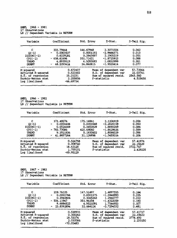
88
SMPL 1965 - 1981 17 Observations LS // Dependent Variable is RETURN
Variable Coefficient Std. Error T-Stat. 2-Tan Sig.
C 333.79444 144.67948 2.3071304 0.042 Q(-l) - 0.0003537 0.0001192 -2.9666371 0.013
DISINC(-l) 0.6229181 0.2843697 2.1905219 0.051 CPI(-l) - 658.61696 351.71421 -1.8725913 0.088 TREND 4.8939519 4.5093083 1.0852999 0.301 DUMMY - 48.5293414 24.860815 -1.9520414 0.077
R-squared 0.672407 Mean of dependent var 57.72564 Adjusted R-squared 0. 523502 S.D. < sf dependent var 22.03761 S.E. of regression 15. 21231 Sum of squared res dd. 2545.560 Durbin-Watson stat 2. 205856 F-statistic 4.515658 Log likelihood -66. 69754
SMPL 1966 - 1982 17 Observations LS // Dependent Variable is RETURN
Variable Coefficient Std. Error T-Stat. 2-Tail Sig.
c 371.48076 175.16961 2.1206919 0.058 Q(-l) - 0.0003408 0.0001548 -2.2020159 0.050
DISINC(-l) 0.6524369 0.3453829 1.8890249 0.086 CPI(-l) - 783.73086 420.69060 -1.8629626 0.089 TREND 9.3921836 5.1930602 1.8086029 0.098 DUMMY - 41.8657264 31.126898 -1.3450016 0.206
R-squared 0.524758 Mean of dependent var 57.41976 Adjusted R-squared 0.308740 S.D. of dependent var 22.15629 S.E. of regression 18.42120 Sum of squared rea lid. 3732.747 Durbin-Watson stat 1.759101 F-statistic 2.429225 Log likelihood -69.95129
SMPL 1967 - 1983 17 Observations LS // Dependent Variable is RETURN
Variable Coefficient Std. Error T-Stat. 2-Tail Sig.
C 219.76125 147.51497 1.4897555 0.164 Q(-l) - 0.0001766 0.0001375 -1.2846993 0.225
DISINC(-l) 0.3940806 0.3045263 1.2940777 0.222 CPI(-l) - 504.11947 351.96354 -1.4323059 0.180 TREND 8.6884523 4.9521091 1.7544953 0.107 DUMMY - 23.8262894 32.664114 -0.7294332 0.481
R-squared 0.518931 Mean of dependent var 57.41717 Adjusted R-squared 0.300263 S.D. of dependent var 22.15622 S.E. of regression 18.53374 Sum of squared res dd. 3778.493 Durbin-Watson stat 2.010086 F-statistic 2.233150 Log likelihood -70.05483
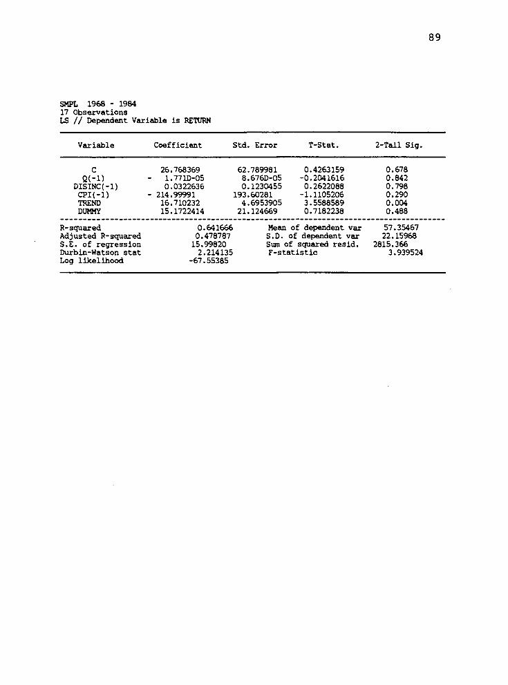
89
SMPL 1968 - 1984 17 Observations LS // Dependent Variable is RETURN
Variable Coefficient Std. Error T-Stat. 2-Tail Sig.
C 26.768369 62.789981 0.4263159 0.678 Q(-l) - 1.7710-05 8.676D-05 -0.2041616 0.842
DISINC(-l) 0.0322636 0.1230455 0.2622088 0.798 CPI(-l) - 214.99991 193.60281 -1.1105206 0.290 TREND 16.710232 4.6953905 3.5588589 0.004 DUMMY 15.1722414 21.124669 0.7182238 0.488
R-squared 0. 641666 Mean . of dependent var 57.35467 Adjusted R-squared 0.' 478787 S.D. of dependent • var 22.15968 S.E. of regression 15.' 99820 Sura ( sf squared res id. 2815.366 Durbin-Watson stat 2. 214135 F-statistic 3.939524 Log likelihood -67. 55385
90
APPENDIX C
DATA FOR ECONOMETRIC MODEL ESTIMATION
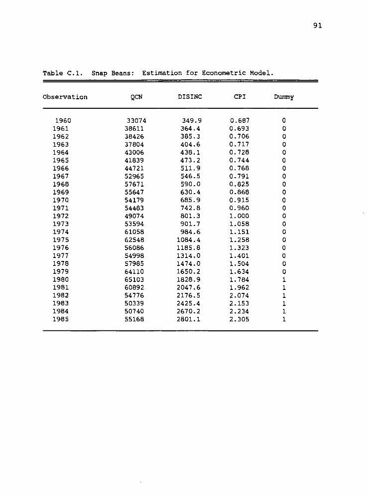
MM
MI-
»M
MM
I-'M
!-'l-»
l-'M
I-'l-'t-
'H'l-'l-'h
-'l-'l--
>l-'>
-'l-'
tji<
iCJK
)MO
»i)a
)--J
a>
ui*
'ijj(o
t-'o
<i)o
o-j<
ntn
it»
.LJM
i-'2
o
cr
en
(D
rt
I—
O
P
(D n
Lnoo*>
-O(-
n^~
J^-c
r>M
i-'U
JU
3^.^
ui~
jM^-i-'C
0-J
CD
00
t-
'-~
ico~
JC
Di-'t-»
iD<
DO
oiO
LnO
ir^M
(T>
o>
vo-J
Oooooi^
(r»
cr>
*^cij~
i(D
oi-'O
ovD
a)*
>L
niD
~ja
)-~
i*>
.~j(T
iMC
JO
oio
H*
00ovD
CT
»N
J0JO
Lna)(
r>aJ00it^i*
'ijJvD
~j»
->uii-'»D
a>
*»cT
>i-' o
IO
Ui
3
•a
0)
(D
0)
3
CO n
M
rt
NJN
JM
MtO
H'M
I-'
ooa^
ji.i
-'ooocr'*
' (-
•otn
a^
-jooo*'
CJ
t-1
O
VO
VD
H«
00
CO
00 o
^
l/l
^ ^
t-J
-J
(TN
o>
en
en
•P* 0
0
CJ
VD
**
to o
n o o
CT>
U
) ^
- ^
. *>
• 0
J U
) ~J
U
J O
00
0>
^
. LO
00 ^
un
*>■
^5
i-'M
4^tn
CT
>vD
MO
oooit>
.<r>
--JLJO
ovo*>
.oi/iii)N
j(-'<
riu)i&
- vO
WM
MM
I-»l-»l-
,»-'l-*l-'l-»
l-»»-»
l-*O
OO
OO
OO
OO
OO
o
(jjM
t-,o
M)~
ja>
Ln^cJM
f->
ooii>
u)o
ooo~
i~j~
j^j~
j-Jcr>
a\
ou)(
ji-J
cr>
ooojo
oM
muiL
nocriH
-'or>
tovocr>
*'iot-
'OvD
<x)
ai*
>.o
j^N
J4
i.^^i-'U
JO
oi-'O
oo
OL
no
ou
ii-'C
D^o
o-J
cr>
u)-
j
a
M
CO
z
o
o
p>
rt
H-
O
P
O m
o o D o 3
<b
rt o o a
ID
MO
OO
OO
OO
OO
OO
OO
OO
OO
OO
O
VO
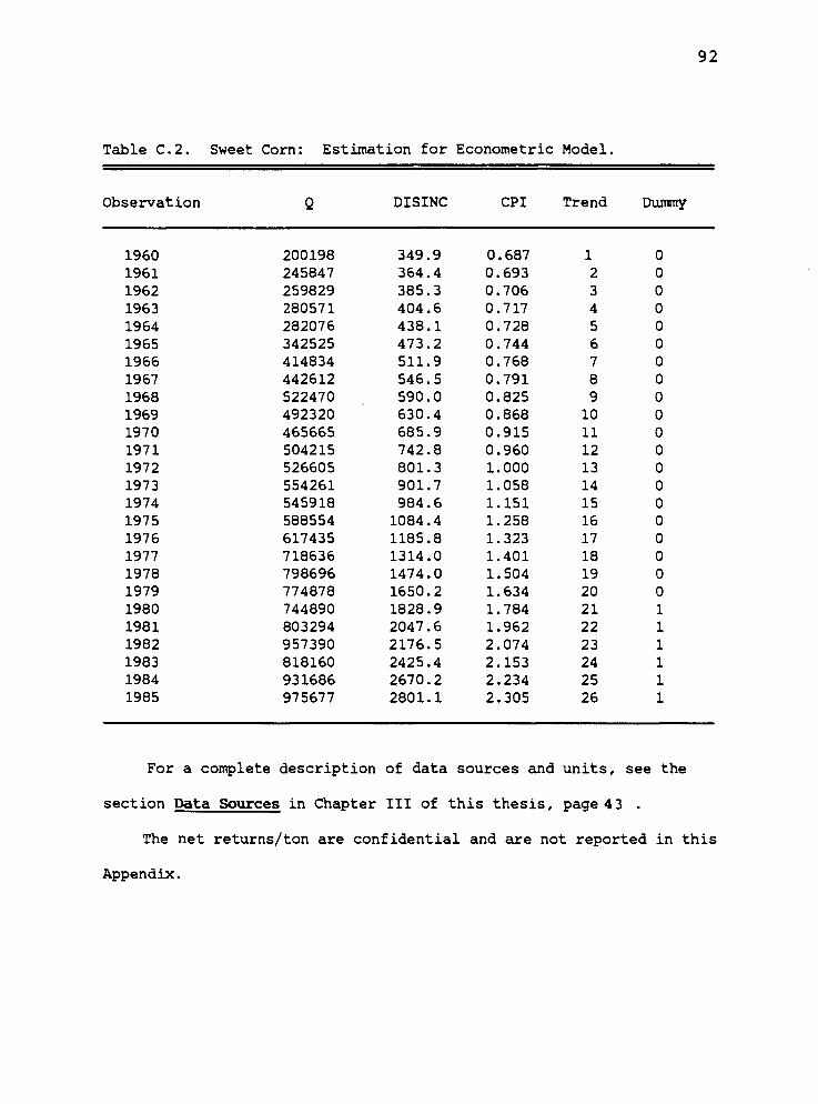
92
Table C.2. Sweet Corn: Estimation for Econometric Model.
Observation Q DISINC CPI Trend Dummy
1960 200198 349.9 0.687 1 0 1961 245847 364.4 0.693 2 0 1962 259829 385.3 0.706 3 0 1963 280571 404.6 0.717 4 0 1964 282076 438.1 0.728 5 0 1965 342525 473.2 0.744 6 0 1966 414834 511.9 0.768 7 0 1967 442612 546.5 0.791 8 0 1968 522470 590.0 0.825 9 0 1969 492320 630.4 0.868 10 0 1970 465665 685.9 0.915 11 0 1971 504215 742.8 0.960 12 0 1972 526605 801.3 1.000 13 0 1973 554261 901.7 1.058 14 0 1974 545918 984.6 1.151 15 0 1975 588554 1084.4 1.258 16 0 1976 617435 1185.8 1.323 17 0 1977 718636 1314.0 1.401 18 0 1978 798696 1474.0 1.504 19 0 1979 774878 1650.2 1.634 20 0 1980 744890 1828.9 1.784 21 1 1981 803294 2047.6 1.962 22 1 1982 957390 2176.5 2.074 23 1 1983 818160 2425.4 2.153 24 1 1984 931686 2670.2 2.234 25 1 1985 975677 2801.1 2.305 26 1
For a complete description of data sources and units, see the
section Data Sources in Chapter III of this thesis, page 43 .
The net returns/ton are confidential and are not reported in this
Appendix.