'.

J. TECHNICAL WRITING AND COMMUNICATION, Vol. 22(1) 39·52,1992

THE ACOUSTICAL PRESENTATION OF TECHNICAL INFORMATION

GEORGE A. BARNETT State University of New York at Buffalo

ABSTRACT

This article advocates listening to technical information in much the same way as scientists and engineers currently look at graphics in order to gain an understanding of the relations among variables. It specifies a number of potential benefits of this approach. 1) lbe ability to hear data may contribute to the greater understanding of the relationships that lie within data. This may lead to alternative theoretical interpretations and explanations. 2) Listening to the data may produce a greater long.term understanding. 3) It will facilitate the understanding of technical information by individuals whose dominant learning modality is acoustic rather than visual. 4) Acoustic data analysis is ideally suited for the analysis of processual data. The article provides a demonstration of the presentation of acoustic information with data on the frequency of television viewing, 1950·1988.

In 1973, F. J. Anscombe wrote [1, p. 17],

Most textbooks on statistical methods, and most statistical computer programs, pay too little attention to graphs. Few of us escape being indoc­trinated with thcse notions:

(1) numerical calculations are exact, but graphs are rough; (2) for any particular kind of statistical data there is just one set of calcula­

tions constituting a correct statistical analysis; (3) performing intricate calculations is virtuous, whereas actually looking

at the data is cheating. A computer should make both calculations and graphs. Both sort of outputs

should be studies; each will contribute to understanding. Graphs can have various purposes, such as: (i) to help us perceive and

appreciate some broad features of the data, (ii) to let us look behind those broad features and see what else is there.

39

© 1992, Baywood Publishing Co., Inc.

40 I BARNETI

Anscombe's statement supporting the use of graphics nearly two decades ago seems to have had a profound impact on technical communication. Today, it is unthinkable not to use graphic displays of technical data. For example, when studying the relationship between two variables, X and Y, with regression analysis, the examination of scatterplots is imperative. Further, today, when reporting the results of even the simplest quantitative research, one is obligated to provide graphic displays of the findings. This may account for the wide-spread use of computer graphiCS programs such as Harvard Graphics.

What Anscombe wrote nearly twenty years ago about the role of visual displays for data may be said today about the use of auditory signals. This article advocates listening to technical information in much the same way as we currently look at graphs in order to gain an understanding of technical material.

You see, any aspect of a piece of music can be expressed as a sequence of pattern of numbers, enthused Richard. "Numbers can express the pitch of notes, the length of notes, patterns of pitches and lengths ...

"You mean tunes," said Reg [2, p. 30].

It is a relatively easy matter to convert a sequence of numbers, i.e., data, into a tune, such that each data point represents a specific tone or note in the tune. In other words, the technical communicator must specify a functional relationship, a one-to-one correspondence, between the value of the data point and some property of the corresponding tone, such as frequency or volume. The series of tones, the tune, may then be created through a simple synthesizer, such as the sound chip available on almost all personal computers. The audience can then simply listen to the information in the same manner as it would look at a graph. How this may be accomplished will be discussed later.

ADVANTAGES OF ACOUSTICAL ANALYSIS

Acoustical data analysis has many potential advantages, including

1. Acoustical data uses an additional channel other than visual. It has long been known that redundancy of information across sensory channels produces increments in learning [3-7]. This ability to simultaneously see and hear information may contribute to greater understanding of the relationships that lie within data. This suggests that acoustical information may also be used in conjunction with graphics.

2. Because analysts are using a different sense, they may be able to dis­criminate alternative patterns that they might not perceive simply by looking at graphic displays. This may facilitate the recognition of sub­tle relations and may lead to alternative theoretical interpretations and explanations.

3

4

:les )n. 'or Y, ve. lve lay rrd

lyS

tes at

) a In " a rty .he lip to be

ng ~ls

~ee

he on

is­by Ib­nd

ACOUSTICAL PRESENTATION OF TECHNICAL INFORMATION / 41

Late 20th century American society is marked by a heavy reliance on the processing of visual information. Perhaps the extensive use of this channel has caused our visual pattern recognition ability to become desensitized. Also, it may have caused our ability to discriminate in other channels to deteriorate. The use of auditory data analysis rather than visual may provide insights unlike interpretations suggested by the visual.

3. Listening to technical information may produce a greater long-term under­standing of the patterns in the data. Children learn nursery rhymes and songs that they can recite (or sing) word for word, without error, as adults. This ability to retain information may be due to the use of the auditory channel. This increased retention may improve our ability to recognize patterns in the data and facilitate our understanding.

4. People differ in their learning modalities-the sensory channel through which they receive and retain information [8, 9]. The three learning modalities that have shown the greatest utility are the visual, auditory, and kinesthetic. Differences in modality strengthS among individuals can be attributed to differences in the efficiency of the sensory pathways. Thus, an individual's dominant modality is that channel through which information is processed most efficiently. In extreme cases, an individual may be blind or deaf and not able to process visual or auditory information. When visual and auditory signals are presented simultaneously, subjects generally respond to the visual input and are often unaware that an auditory signal has occurred. This occurs despite the fact that research has shown that auditory stimuli may be processed more rapidly than visual stimuli [10]. Further­more, cultural differences have been found to correlate with learning modalities [11].

Technical communication has primarily made use of only the visual modality. This has perhaps deprived those individuals whose dominant learning modality is auditory from gaining an understanding of the patterns within technical data. Further, individuals from cultures whose dominant learning modality is verbal may be restricted by norms which emphasize the visual modality for scientific and technical information. The acoustic presentation of technical information will allow auditory learners the oppor­tunity to use their dominant learning modality and deal with displays as efficiently as visual learners.

5. Acoustic presentations are ideally suited for the analysis of processual data. One advantage of graphics is the ability to simultaneously present an entire process. By presenting all the information at one time, however, processual aspects are obscured. Other than presenting a line on a graph that represents time, the processual component is removed from the data presentation. The acoustic presentation of data, however, forces one to listen in a time-de­pendent fashion, one tone after another. In order to add this dimension visually, a film or video tape would be required.

42 I BARNETT

The above discussion raises the question, "What do we need to know about the human perception of sound in order to effectively present information acoustic­ally?" In other words, how should the tunes sound in order to maximize the benefits for listeners? The section that follows reviews the literature on frequency thresholds of human hearing. Based on this information, an example is presented using the frequency of tones to indicate the value of certain variables over time.

HUMAN PERCEPTION OF SOUND FREQUENCY

The frequency limits of human hearing generally range from approximately 20 Hz (Hertz) to 20,000 Hz for normal young people, although this range is dependent upon the intensity (volume) of the tone [12V These limits arc for 80 decibels (dB).2 With increased intensity the range may be extended to about 10 Hz to 23,000 Hz. Above 23,000 Hz, pain becomes the limiting factor.

Through a series of experiments, Shower and Biddulp determined the differen­tial threshold or the just notable difference (IND) for human hearing [13]. The JND is significant because it defines the threshold or the change in frequency required for a listener to detect a difference between two tones. At 30 dB, they determined that the JND was a constant between 2 and 3 (Hz), in the 60 to 1000 Hz frequency range. For higher frequencies, the IND increases rapidly. Above 1000 Hz, the relative IND (Mlf) is constant [14].

More recently, Wier, Jesteadt, and Green replicated the Shower and Biddulp experiments using pulses produced with electronic switches rather than sliding tones [15]. Overall, the results were similar. However, Wier et al. found that the thresholds were smaller at lower frequencies (only about 1 Hz at 40 dB) and considerably larger at high frequencies than for the same values used by Shower and Biddulph. In summary, the listener cannot detect differences below lor 2 Hz between tones.

How long should the tones be? Yost and Moore found that listeners could not discriminate the frequencies of sounds if the rate of presentation exceeded ten tones per second [16]. This suggests that spectral prOfiles that exceed 100 msec (milliseconds) cannot be detected [12]. A period of silence of at least 2 msec is also required for the recognition of the presence of two separate tones [17].

The ability to detect small changes in frequencies requires training [18]. Train­ing listeners to use auditory information involves introducing the concept and familiarizing them with the types of changes and patterns for which they should listen. Then they are asked to attempt to detect changes in the frequencies of tones

1 Hertz (Hz) is a unit of frequency equal to one cycle (wave) per second. Frequency is the number of waves, measured from peak to peak, per unit time.

2 Decibel (dB) is a unit for expressing relative volume. It is the ratio of two amounts of acoustic signal power, equal to ten times the common logarithm of this ratio.

a r c i: r s 11 j

ti

n [ Ii s. t(

CI

It

P

TI pr pc ff( fIf

tle c­~e

~y

~d

ly is )r Jt

l­

Ie y y o e

p g e d r z

t 1

ACOUSTICAL PRESENTATION OF TECHNICAL INFORMATION I 43

and define a pattern in the sequence. Initially, the patterns should be easily recognizable and the difference in frequency substantial. For example, the listener could be asked to listen for fluctuations in frequency in a series of tones where one is 200 Hz and another is 2,500 Hz. As the listener skills improve, the difference is reduced. Eventually, the training will be a series of exercises to sharpen skills. The sensation level and the decibel level used for the training sessions should be the level most comfortable for the listener. There is no optimal sensation level [18]. After approximately fifteen to twenty hours of training, listeners improve their detec­tion skills by a factor of 8 to 10 just detectable values or just notable differences.

Research indicates that there is a direct relationship between the listener's musical training and his/her ability to detect changes in the frequency of tones [18]. Musicians do it better than non-musicians because they have been trained to listen to the frequenCies of tones. To present auditory information one cannot simply listen to the data. One must learn how to listen. As with music, the ability to analyze data acoustically improves with practice.

PROCEDURES FOR ACOUSTIC DATA PRESENTATION

One can present data acoustically by using an IBM or IBM-compatible personal computer with a sound chip, a speaker, and the Nortoll Utilities [19] software with the Beep Utility. Nortoll Utilities controls the production of tones with three parameters or switches:

1. The frequency of the tone is determined simply by IFo where n equalS the frequency of the tone. A tone of 500 Hz would be produced by !F500.

2. The tone's duration is control by !Do where n equals the length of the tone in "clock ticks" each 1/18 of a second, or 55.56 msec. As indicated above, a duration of at least 100 msec or two clock ticks is optimal for acoustic data analysis. This length would be controlled by /D2.

3. Silence or the wait between tones can be produced by IWo. Again, the length of the silence between tones is measured in clock ticks of 1/18 of a second. Any wait greater than zero is optimal. A silence of one clock tick would be indicated by /Wl.

A typical line from a data file might look like

/F500 /D2/W1

This would produce a 500 Hz tone for 111.12 msec and then wait 55.56 msec until producing the next tone. Thus, to acoustically examine a single variable over n points in time, one would create a file n lines long. Each line indicates the frequency and the duration of the tone and wait between each tone. Beep is very flexible and allows for multiple tones per line. This makes it possible to listen to more than one variable per case.

44 / BARNETT

To listen to a tune, one runs "Beep" by simply typing Beep filename.

AN EXAMPLE­SEASONALITY IN TELEVISION VIEWING

The data used to demonstrate the utility of presenting technical information acoustically come from A. C. Nielsen. It describes the frequency of television viewing by the average American household expressed at monthly intervals for the period September 1950 to August 1989. There are 460 data pOints. The lowest amount of viewing occurs during July 1950: 3 hours and 31 minutes. The peak occurs during January 1985: 7 hours and 58 minutes. The data, presented in Table 1, were transformed into minutes for analysis.

As reported by Barnett, Chang, Fink, and Richards, frequency of television viewing may be described by two components, one describing the seasonal variation in viewing and another the diffusion of the medium [20]. Mathe­matically, the data may be modelled by equation 1:

Yl = B1(cos(B2(t - B3)) + (B4/(1+B5(exp (-B6 t»» + B7 1

where

Yl = B1(cos(B2(t = B3») 1.1

describes the seasonal component, and

Yl = B4/(1+B5(exp (-B6 t») 1.2

is a logistic describing the diffusion of television viewing. The B's are parameters which determine the shape of the curve. They are explained in Barnett, et al. [20].

The model fits the data extremely well.3 The residuals are normaIly distributed and can be explained by social factors, such as the FCC freeze on broadcast affiliates in the early 1950s, the growth of cable television in the 1970s, and the decrease in television viewing in recent years in favor of the use of VCRs.

Three separate tunes are presented for these data: one for the values predicted from the mathematical model (Tune 1); another with the actual frequency of television viewing (Tune 2); and a third with the residuals (Tune 3). The data were converted to tones by changing the units of the values from minutes to Hz. They are available on computer disk from the author upon request.

Since the values of the residuals « 20 minutes) are typically below the fre­quency threshold of human hearing « 20 Hz), the overall mean value (351.55 minutes) is added to the data. This has the additional advantage of placing this tune in the same range as the other two tunes. The audience has listened to hearing tones in this range and is thus more sensitive to these frequencies.

3 The results of tbe test of the theoretical model are presented in Barnett, et a!. [20].

(

r

on on 'or ~st

ak in

)n

al e-

1

.1

.2

rs

'J. :d

st le

:-5 s g

ACOUSTICAL PRESENTATION OF TECHNICAL INFORMATION / 45

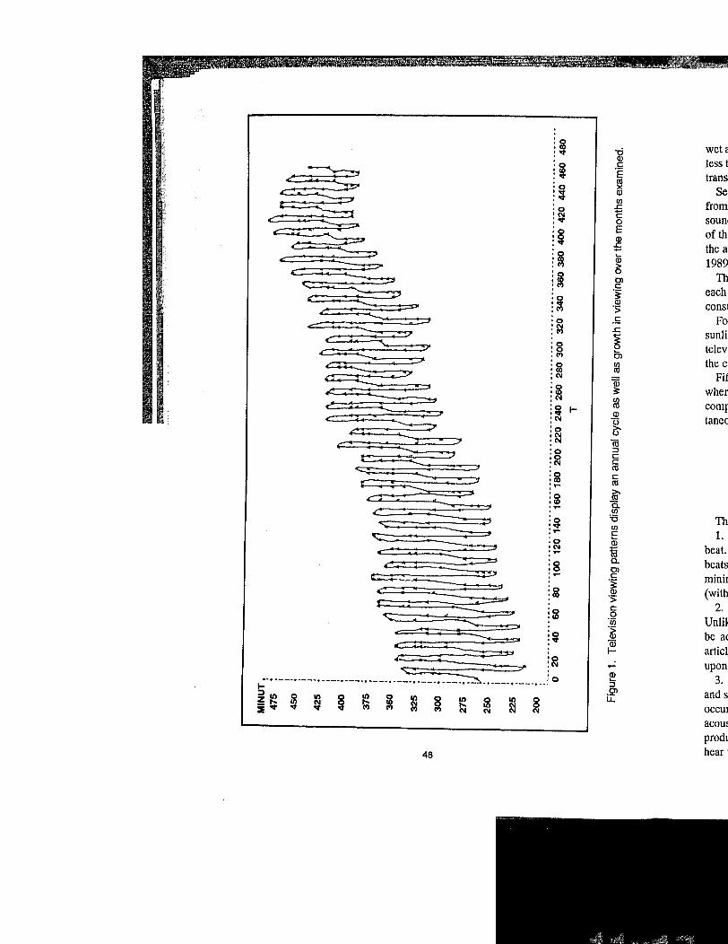
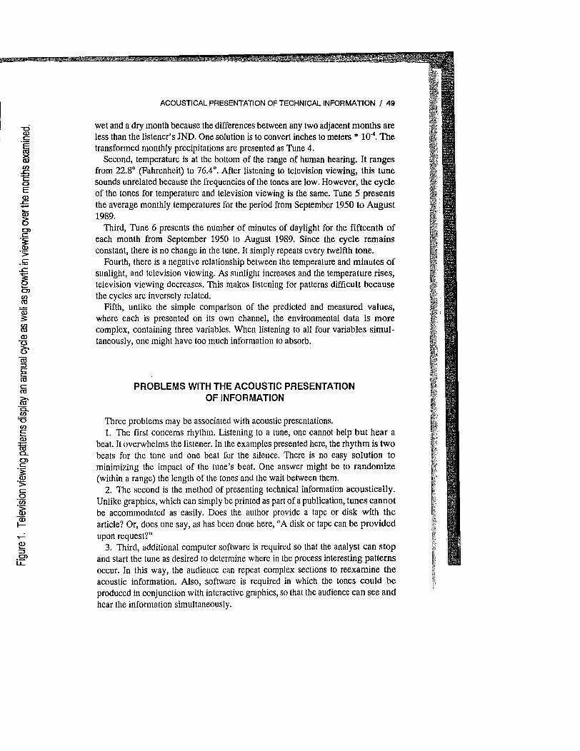
With both the theoretical model and actual data, the listener should hear the two components of the model. The first is the annual cycle in viewing. This is a twelve month or tone cycle. Starting in September, the frequency of the tone rises for four or five tones then declines for seven or eight. The second component is the diffusion or growth in television viewing. Since the frequency of the tones is isomorphic with the frequency of viewing, the tune starts out with low tones. The tones rise slowly and then rise more quickly as viewing grows rapidly. Finally, they rise more slowly and level off at a higher frequency.

When listening to the actual viewing data, one notices that the tones begin to drop at the end. This is due to the recent decline in television viewing in favor of the use of VCRs. The actual viewing data is graphically displayed as a function of time (in months) in Figure 1.

When listening to the residuals, one hears a generally downward trend in the tones. The greatest positive residuals occur early in the data and the greatest negative residuals at the end. One can easily make out a negative trend. Indeed, the correlation between residuals and time is -.26, suggesting that the theoretical model needs an additional component to model the disadoption of television viewing [21, 22].

MORE COMPLEX TIME

More complex presentations of acoustic information require additional equip­ment. For example, one could produce a tune with the theoretical model in one channel and the actual data simultaneously in another. The audience could then listen in stereo to the predicted values in the right channel while listening to the measured values in the left. They could listen for differences between the channels, Le., errors in the theoretical model. However, presentation of multiple tones simultaneously requires either a computer with a polyphonic board, such as an Amiga or a Next, or a mixing board and a multi-channel tape recorder. Cur­rently, software is being written for an Amiga for the simultaneous presentation of multiple tones.

An interesting application of complex acoustic data comes from Barnett et a1. [20]. In attempting to identify the underlying determinants of the seasonal pattern in viewing, they analyzed television viewing, the number of minutes of daylight, the mean monthly temperature, and the mean monthly precipitation. The results of a spectral analysis indicated strong relationships among the variables, suggest­ing that television viewing may be a function of the weather. To gain a better understanding of how environmental factors impact upon television viewing, these four variables could be presented acoustically.

This example poses a number of interesting problems. First, precipitation is out of the range of human hearing. It is reported in inches by NOAA and ranges from .54 to 4.15 inches [23,24]. Even if one added a constant to bring the series into the range of human hearing, the listener would not be able to discriminate between a

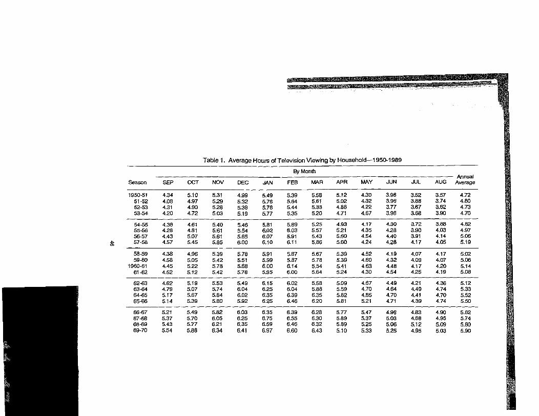
Table 1. Average Hours of Tefevision Viewing by Household-1950-1989

By Month Annual

Season SEP OCT NOV DEC JAN FEB MAR APR MAY JUN JUL AUG Average

1950-51 4.34 5.10 5.31 4.99 5.49 5.39 5.58 5.12 4.30 3.96 3.52 3.57 4.72 51-52 4.08 4.97 5.29 5.32 5.76 5.64 5.61 5.02 4.32 3.96 3.88 3.74 4.80 52-53 4.31 4.90 5.28 5.38 5.76 5.44 5.33 4.88 4.22 3.77 3.67 3.82 4.73 53-54 4.20 4.72 5.03 5.19 5.77 5.35 5.20 4.71 4.67 3.98 3.68 3.90 4.70

54-55 4.38 4.61 5.40 5.46 5.81 5.89 5.25 4.93 4.17 4.30 3.72 3.88 4.82 55-56 4.28 4.81 5;61 5.54 6.02 6.03 5.57 5.21 4.35 428 3.90 4.03 4.97 56-57 4.43 5.07 5.61 5.65 6.07 5.91 5.43 5.60 4.54 4.40 3.91 4.14 5.06

~ 57-58 4.57 5.45 5.85 6.00 6.10 6.11 5.86 5.60 4.24 4.28 4.17 4.05 5.19 m

58-59 4.38 4.96 5.39 5.78 5.91 5.87 5.67 5.39 4.52 4.19 4.07 4.17 5.02 59-60 4.58 5.05 5.42 5.51 5.99 5.87 5.78 5.39 4.60 4.32 4.09 4.07 5.06

1960-61 4.45 5.22 5.78 5.68 6.00 6.14 5.54 5.41 4.63 4.48 4.17 4.20 5.14 61-62 4.52 5.12 5.42 5.78 5.95 6.00 5.64 5.24 4.30 4.54 425 4.19 5.08

62-63 4.62 5.19 5.53 5.49 6.15 6.02 5.58 5.09 4.67 4.49 4.21 4.36 5.12 63-64 4.79 5.07 5.74 6.04 6.25 6.04 5.88 5.59 4.70 4.64 4.49 4.74 5.33 64-65 5.17 5.67 5.84 6.02 6.35 6.39 6.35 5.82 4.85 4.70 4.41 4.70 5.52 65-66 5.14 5.39 5.80 5.92 6.25 6.46 6.20 5.81 5.21 4.71 4.39 4.74 5.50

66-67 5.21 5.49 5.82 6.03 6.35 6.39 6.28 5.77 5.47 4.96 4.83 4.90 5.62 67-68 5.37 5.70 6.05 6.25 6.75 6.55 6.30 5.89 5.37 5.03 4.68 4.95 5.74 68-69 5.43 5.77 6.21 6.35 6.59 6.46 6.32 5.89 5.25 5.06 5.12 5.09 5.80 69-70 5.54 5.88 6.34 6.41 6.97 6.60 6.43 5.10 5.33 5.25 4.95 5.03 5.90

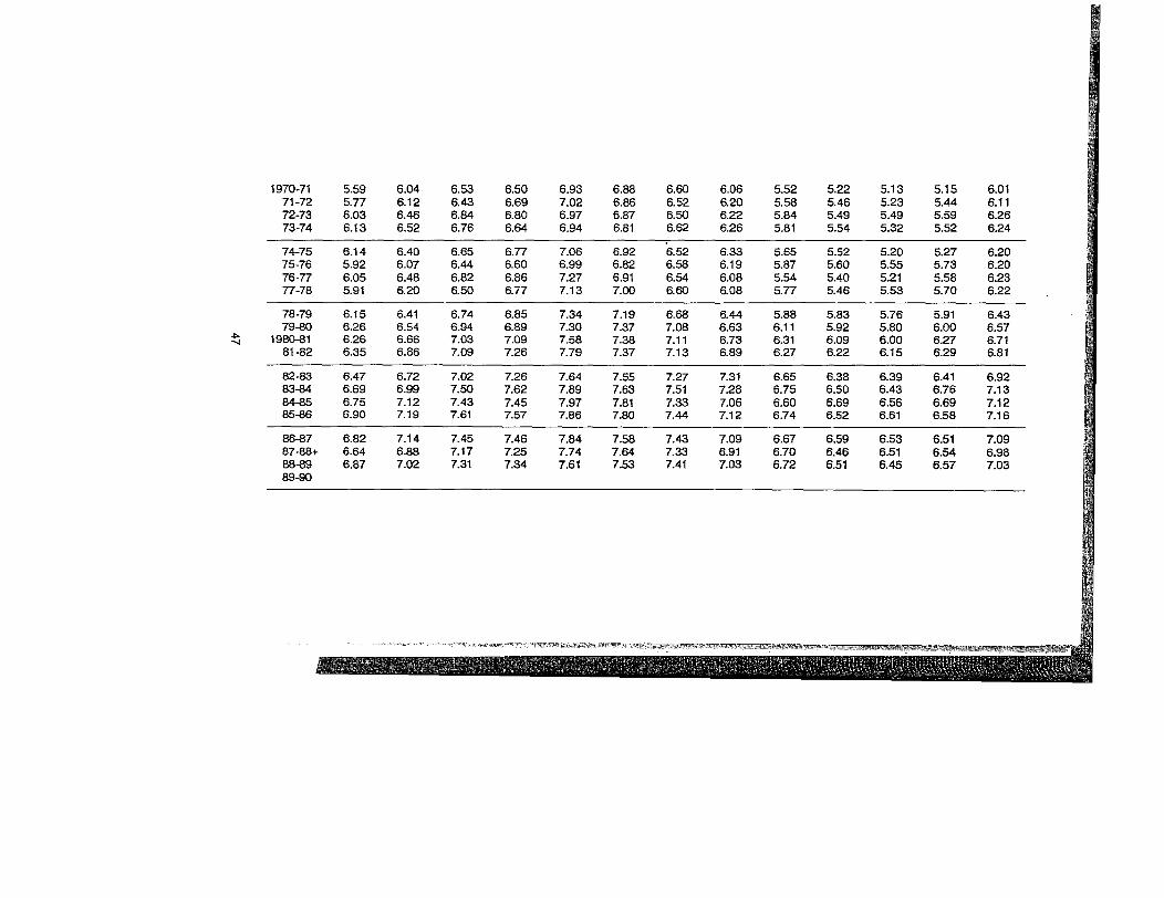
1970-71 5.59 6.04 6.53 6.50 6.93 6.88 6.60 6.06 5.52 5.22 5.13 5.15 6.01 71-72 5.77 6.12 6.43 6.69 7.02 6.86 6.52 6.20 5.58 5.46 5.23 5.44 6.11 72-73 6.03 6.46 6.84 6.80 6.97 6.87 6.50 6.22 5.84 5.49 5.49 5.59 6.26 73-74 6.13 6.52 6.76 6.64 6.94 6.81 6.62 6.26 5.81 5.54 5.32 5.52 6.24

74-75 6.14 6.40 6.65 6.77 7.06 6.92 6.52 6.33 5.65 5.52 5.20 5.27 6.20 75-76 5.92 6.07 6.44 6.60 6.99 6.82 6.58 6.19 5.87 5.60 5.55 5.73 6.20 76-77 6.05 6.48 6.82 6.86 7.27 6.91 6.54 6.08 5.54 5.40 5.21 5.58 6.23 77-78 5.91 6.20 6.50 6.77 7.13 7.00 6.60 6.08 5.77 5.46 5.53 5.70 6.22

78-79 6.15 6.41 6.74 6.85 7.34 7.19 6.68 6.44 5.88 5.83 5.76 5.91 6.43 79-80 6.26 6.54 6.94 6.89 7.30 7.37 7.08 6.63 6.11 5.92 5.80 6.00 6.57

-1>0 1980-81 6.26 6.66 7.03 7.09 7.58 7.38 7.11 6.73 6.31 6.09 6.00 6.27 6.71 ..... 81-82 6.35 6.86 7.09 7.26 7.79 7.37 7.13 6.89 6.27 6.22 6.15 6.29 6.81

82-83 6.47 6.72 7.02 7.26 7.64 7.55 7.27 7.31 6.65 6.38 6.39 6.41 6.92 83-84 6.69 6.99 7.50 7.62 7.89 7.63 7.51 7.28 6.75 6.50 6.43 6.76 7.13 84-85 6.75 7.12 7.43 7.45 7.97 7.81 7.33 7.06 6.60 6.69 6.56 6.69 7.12 85-86 6.90 7.19 7.61 7.57 7.86 7.80 7.44 7.12 6.74 6.52 6.61 6.58 7.16

86-87 6.82 7.14 7.45 7.46 7.84 7.58 7.43 7.09 6.67 6.59 6.53 6.51 7.09 87-88+ 6.64 6.88 7.17 7.25 7.74 7.64 7.33 6.91 6.70 6.46 6.51 6.54 6.98 88-89 6.87 7.02 7.31 7.34 7.61 7.53 7.41 7.03 6.72 6.51 6.45 6.57 7.03 89-90

ii ,; wet~ 0> less t 1~ c: ·E trans «1 1; ~ Se III from :0 .c

:~ "E SQun, 0

i§ E ofth 0> -S the a Ii ...

1989 0>

~ j~ Cl Th

c: each

1~ .~

0> cons! .s: '0 .s Fo :f;:! .c sunJi

~~ ~ telev ... Cl

the c. ;~ III «1

Fif :N Qi :f6 ~ wher

:N al comI ;~ I-0>

lanee :N "0 :0 t>' :~ "'iii :0 ::J .0 c: :N c:

«1 ;~ c:

«1 :'"" ~ :f6 Ci :'"" III

:~ '6 Th III :,... c: 1. :0 ... 0>

beat. 'N i :,... :8 Q. beats 0)

minil :.- c:

~~ .~

(with 0> .s: 2. :f6 c:

0 Unm ·iii

~~ .~

be a( Qi

articl · l-· '0 upon :N or-· 0>

3. · ,0 ... .... ---- .. ----. ---- .. ----. ----t --__ • ____ • ___ ... __ -. ---- .. ----. --, ::J I-0) and s ;:)."

~ ." § ~ I ."

~ ." ~ ~ 8 u:: ~tt N f;:! "'" OCCUI "It "It N N N N :e acoUl prodl

48 hear 1

ACOUSTICAL PRESENTATION OF TECHNICAL INFORMATION J 49

wet and a dry month because the differences between any two adjacent months are less than the listener's JND. One solution is to convert inches to meters * 10-4

• The transformed monthly precipitations are presented as Tune 4.

Second, temperature is at the bottom of the range of human hearing. It ranges from 22.8° (Fahrenheit) to 76.4°. After listening to television viewing, this tune sounds unrelated because the frequencies of the tones are low. However, the cycle of the tones for temperature and television viewing is the same. Tune 5 presents the average monthly temperatures for the period from September 1950 to August 1989.

Third, Tune 6 presents the number of minutes of daylight for the fifteenth of each month from September 1950 to August 1989. Since the cycle remains constant, there is no change in the tune. It simply repeats every twelfth tone.

Fourth, there is a negative relationship between the temperature and minutes of sunlight, and television viewing. As sunlight increases and the temperature rises, television viewing decreases. This makes listening for patterns difficult because the cycles are inversely related.

Fifth, unlike the simple comparison of the predicted and measured values, where each is presented on its own channel, the environmental data is more complex, containing three variables. When listening to all four variables simul­taneously, one might have too much information to absorb.

PROBLEMS WITH THE ACOUSTIC PRESENTATION OF INFORMATION

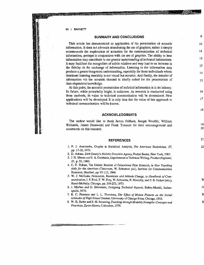
Three problems may be associated with acoustic presentations. 1. The first concerns rhythm. Listening to a tune, one cannot help but hear a

beat. It overwhelms the listener. In the examples presented here, the rhythm is two beats for the tone and one beat for the silence. There is no easy solution to minimizing the impact of the tune's beat. One answer might be to randomize (within a range) the length of the tones and the wait between them.

2. The second is the method of presenting technical information acoustically. Unlike graphics, which can simply be printed as part of a publication, tunes cannot be accommodated as easily. Does the author provide a tape or disk with the article? Or, does one say,_ as has been done here, "A disk or tape can be provided upon request?"

3. Third, additional computer software is required so that the analyst can stop and start the tune as desired to determine where in the process interesting patterns occur. In this way, the audience can repeat complex sections to reexamine the acoustic information. Also, software is required in which the tones could be produced in ccnjunction with interactive graphics, so that the audience can see and hear the information simUltaneously.

50 I BARNETI

SUMMARY AND CONCLUSIONS

This article has demonstrated an application of the presentation of acoustic information. It does not advocate abandoning the use of graphics; rather it simply recommends the exploration of acoustics for the communication of technical information, perhaps in conjunction with the use of graphics. The ability to hear information may contribute to our greater understanding of technical information. It may facilitate the recognition of subtle relations and may lead to an increase in the fidelity in the exchange of information. Listening to the information may produce a greater long-term understanding, especially for those individuals whose dominant learning modality is not visual but acoustic. And finally, the transfer of information via the acoustic channel is ideally suited for the presentation of time-dependent knowledge.

At this point, the acoustic presentation of technical information is in its infancy. Its future, while potentially bright, is unknown. As research is conducted using these methods, its value to technical communication will be determined. New applications will be developed. It is only then that the value of this approach to technical communication will be known.

ACKNOWLEDGMENTS

The author would like to thank James Gillham, Joseph Woelfel, William Richards, James Danowski and Frank Tutzauer for their encouragement and comments on this research.

REFERENCES

1. F. J. Anscombe, Graphs in Statistical Analysis, The American Statistician, 27, pp. 17-21, 1973.

2. D. Adams, Dirk Gently's Holistic Detective Agency, Pocket Books, New York, 1987. 3. J. H. Bloom and S. A. Goldstein, Experiments in Technical Writing, Prodllct Engineer,

31, p. 55, 1960. 4. C. F. Hoban, The Usable Residue of Educational Film Research, in New Teaching

Aids for the American Classroom, W. Schramm (ed.), Institute for Communication Research, Stanford, pp. 95-115,1960.

5. W. J. McGuire, Persuasion, Resistance and Attitude Change, in Handbook of Com­municatioll, I. S. Pool, F. W. Frey, W. Schramm, N. Maccoby, and E. B. Parker (eds.), Rand-McNally, Chicago, pp. 216-252,1973.

6. J. Mathes and D. Stevenson, Designing Technical Reports, Bobbs-Merrill, Indian­apolis, 1976.

7. R. C. Peterson and L. L. Thurstone, The Effect of Motion Pictures on the Social Attitudes of High School Siudelll, University of Chicago Press, Chicago, 1933.

8. W. B. Barbe and R. H. Swassing, Teaching throllgh Modality Strengths: Concepts and Practices, Zaner-Bloser, ColUmbus, 1979.

9

10

11

12

13

14

15

16

17

18

19, 20,

21.

22.

Bal

Go

Bm

Bal

)f acoustic :r it simply , technical ity to hear formation. ncrease in ~tion may :als whose :ransfer of Iltation of

S infancy. :ted using lcd. New proach to

William nen! and

Cian, 27,

·k,1987. '!:ngilleer,

Teachillg L1nication

ofCom­er (eds.),

, Indian-

e Social

eptsalld

ACOUSTICAL PRESENTATION OF TECHNICAL INFORMATION / 51

9. R. Dunn, Bias Over Substance: A Critical Analysis of Kavale and Forness' Report on Modality-Based Instruction, Exceptiollal Children, 56, pp. 357-361, 1990.

10. K. Robinson, Visual alld Auditory Modalities and Reading Recall: A Review of the Research, EDRS, 1985.

11. R. Dunn, J. S. Beaudry, and A. Klavas, Survey of Research on Learning Styles, Educatiollal Leadership, 46, pp. 50-58, 1989.

12. W. L. Gulick, G. A. Gescheider, and R. D. Frisina, Hearillg: Physiological Acoustics, Neural Codillg, and Psychoacoustics, Oxford University Press, New York, 1989.

13. E. G. Shower and R. Biddulph, Differential Pitch Sensitivity of the Ear, Journal of the Acoustical Society of America,. 3, pp. 275-287, 1931.

14. J. C. R. Licklider, Basic Correlates of the Auditory Stimulus, in Handbook of Experimelltal Psychology, S. S. Stevens (ed.), Wiley, New York, pp. 985-1040,1958.

15. C. C. Wier, W. Jesteadt, and D. M. Green, Frequency Discrimination as a Function of Frequency and Sensation Level, J oumal of the Acoustical Society of America, 61, pp. 178-184, 1977.

16. W. A. Yost and M. J. Moore, Temporal Changes in a Complex Spectral Profile, Journal of the Acoustical Society of America, 81, pp. 1896-1905, 1987.

17. T. G. Forrest and D. M. Green, Detection of Partially Filled Gaps in Noise and the Temporal Modulation Transfer Functions, Journal of the Acoustical Society of America, 82, pp. 1933-1943, 1987.

18. C. S. Watson, H. W. Wroton, W. J. Kelly, and C. A. Benbasset, Factors in the Discrimination of Tonal Patterns. I. Component Frequency, Temporal Position, and Silent Intervals, Journal of the Acoustical Society of America, 57, pp. 1175-1185, 1975.

19. P. Norton,Nortoll Utilities, (Advanced Edition), 1987. 20. G. A. Barnett, H. S. Chang, E. L. Fink, and W. D. Richards, Seasonality in Television

Viewing: A Mathematical Model of Cultural Processes, Communication Research, 18, pp. 755-772, 1991.

21. G. A. Barnett, E. L. Fink, and M. B. Debus, A Mathematical Model of Academic Citation Age, Commullicatioll Research, 16, pp. 510-531, 1989.

22. H. S. Chang, An Examination of the Diffusion of Innovations: A Mathematical Test of the Adoption and Disadoption Process, paper presented to the International Com­munication Association, Chicago, May, 1991.

Other Articles On Communication By This Author

Barnett, G. A., E. L. Fink, and M. B. Debus, A Mathematical Model of Academic Citation Age, Communication Research, 16, pp. 510-531, 1989.

Goldhaber, G. M. and G. A. Barnett, (eds.), Handbook of Organizational Communication, Ablex, Norwood, New Jersey, 1988.

Barnett, G. A. and G. Siegel, The Diffusion of Computer Assisted Legal Research Systems, Journal of the American Society for Ill/ormatioll Science, 39, pp. 224-234, 1988.

Barnett, G. A. and R. E. Rice, Network Analysis in Riemann Space: Applications of the Galileo System to Social Networks, Social Networks, 7, pp. 287-322, 1985.

52 I BARNETT

Barnett, G. A and C. E. Hughes, Communication Theory and Technical Communication, in Research in Technical Communication, M. G. Moran and D. Journet (eds.), Green­wood Press, Westport, Connecticut, pp. 39-84, 1984.

Barnett, G. A, Applications of Communication Theory and Cybernetics to Technical Communication, Journal of Technical Writing and Communication, 9, pp. 337-347, 1979.

Direct reprint requests to:

Professor George A. Barnett Department of Communication 338 M.F.A.c'-ElIicott Complex University at Buffalo Buffalo, NY 14261

J. T

C( K. "G

R_J Uni

Fer fe\\ tior sen SiOI

the 1

par wo° and the is I

pre Fer fou sub wh gre COl

(

atte pas of] laU

©1'